Early Proceedings of the Alterman Conference 2016 · Topics: Introduction to Clifford algebra Development of Clifford concepts Arbitrary dimension Applications of geometric algebra

Early Proceedings of the Alterman Conference on Geometric Algebra and

Summer School on Kähler Calculus

August 1st to 9th, 2016 Bra ov (Romania)

Honorary Pres ident : Eric Alterman

Editors: Ramon González (edi tor in chief )

Panackal Harikrishnan

Marius Paun

Jose G. Vargas (chairman)

Associate edi tor: Rafa Ab amowicz

Early Proceedings of the Alterman Conference on Geometric Algebra and Summer School on Kähler Calculus

(Final edition)

This electronic edition is in copyright. The editors own the copyright of the edition as a whole. Each author owns the copyright of his articles and is free to publish them in any journal.

This file is published at the website of the Alterman Conference:

http://cs.unitbv.ro/~acami/

and cannot be posted or stored on any other website, except authors’ homepages, without the permission of the editors. Printing this file is only allowed for personal use. Those who try to obtain any economic profit from this edition by any means without permission will be brought to justice.

ISBN: 978-84-608-9911-2

Published on September 21st, 2016

Dear Colleagues,

We wish to thank all authors for their contributions to these Early Proceedings and especially to Mr. Eric Alterman for his financial support to the Conference and Summer School.

For the second time, I am having the pleasant task of editing electronic Early Proceedings. The aim is to make the writings of other participants promptly available to attendants. Book editions of proceedings of many conferences are usually so much delayed that interest in them has substantially decreased by the time they finally appear. In the Early Proceedings, new authors have the opportunity to publish papers that may very well not be accepted in scientific journals, which usually have a limited size and different selection criteria.

We thank very much Professors Rafa Ab amowicz, Nikolay Marchuk, Zbigniew Oziewicz, Waldyr Jr. Rodrigues, José G. Vargas and Dr. Lucy Kabza for reviewing the submitted papers and giving their scientific advice. In some cases, members of the scientific committee and authors have begun a fruitful dialogue like between master and student. The beauty of teaching lies in the fact that the experienced (generally elder) masters can transmit to the inexperienced (generally younger) students knowledge that cannot be found in the literature. There are occasions when the breaking of this chain causes knowledge to be lost, and later generations must then discover what older generations already knew. Therefore, I want to thank Prof. José G. Vargas for his main role as master of the Kähler calculus during the Summer School of the Alterman Conference. Without him, it might fall into oblivion. Fortunately, he has removed the dust that covered the writings of Erich Kähler on differential calculus, which were never translated into English. He has summarized their contents for us in the Notes on the Kähler calculus for the Summer School included in these Early Proceedings, which we hope will be very useful material for our learning. Moreover, he has assured that there will be a more polished and efficient version of the same material in some other venue, be it a book or a second Alterman Summer School, or both.

Ramon González Calvet,

September 21st, 2016

EARLY PROCEEDINGS OF THE ALTERMAN CONFERENCE 2016

Foreword to the Notes on the Kahler calculusfor the Summer School

During months prior to the event Alterman Conference on Clifford Algebra andSummer School on Kahler Calculus, I wrote the chapters that follow in responseto the non-availability in English of comparable contents. There were meantto be instrumental in preparing knowledgeable mathematicians to absorb thematerial and share with me the task of teaching them at the Summer School.

Things did not go as planned, owing to different reasons, which need notbe reported here. Through polishing, simplification and eliminations, futureversions of this material will be presented almost as if for use in a college course.For the moment and in spite of the many typos that I am sure still remain,nothing can be lost from having them as an alternative presentation of a largepart of the original German papers.

Chapter 1 is an introduction that can be ignored without consequence. Inthe remaining chapters, we observe that no differential forms valued in tangentstructures are used, observation which is of the essence in understanding thiscalculus. The material presented is certainly contained as particular case of hiscalculus of tensor-valued differential forms, but he gave no application for thismore general valuedness other than proposing a very cumbersome “Kahler-Dirac”equation, for which we have no use.

I want to thank you all for your participation and I apologize for any defi-ciencies that should not have occurred. This event encountered severe intrinsicdifficulties almost until a few weeks prior to its taking place. In order to avoidthem, a second Alterman Summer School would not include a Conference in par-allel. It would rather consist of four days of exclusive teaching of as many relatedtopics: (a) the required basic Clifford algebra, (b) Kahler algebra (it is Cliffordalgebra, but the fact that its elements are differential forms makes a great differ-ence), (c) Kahler calculus proper and (d) Kahler’s quantum mechanics. I hopethat you do not fail to realize the opportunity you may have to learn this mostpowerful calculus now that you are aware of its existence. Of particular relevancefor the occurrence of an Alterman 2 event is that we find mathematicians whocan teach this calculus without resort to non-scalar valuedness. If you can thinkof such candidates, please let me know as soon as possible.

It was a great pleasure to interact with you. Kind regards.

Jose G. Vargas


INDEX

SUMMER SCHOOL

Phase 1: Introduction to Geometric Algebra

Rafa Ab amowicz: On the structure theorem of Clifford algebras…………………….. 3

Rafa Ab amowicz: A tutorial on CLIFFORD with eCLIFFORD and BIGEBRA. A Maple package for Clifford and Grassmann algebras (abstract)………………………………. 13

Ramon González: Application of geometric algebra to plane and space geometry …… 15

Ramon González: The exterior calculus ………………………………………….......... 43

Phases 2 and 3: Kähler calculus and its applications

José G. Vargas: Notes on the Kähler calculus for the Summer School

Chap. 1. Perspective on the Kähler calculus for experts in Clifford analysis…… 61

Chap. 2. Kähler algebra ………………………………………………………… 71

Chap. 3. Kähler differentiations ………………………………………………… 86

Chap. 4. Relativistic Quantum Mechanics …………………………………….. 107

Chap. 5. Lie differentiation and angular momentum ………………………….. 126

Chap. 6. Conservation in Quantum Mechanics. Beyond Hodge’s theorem …… 145

ALTERMAN CONFERENCE

Special topic: Grassmann's legacy with emphasis on the projective geometry

Oliver Conradt: Projective, Clifford and Grassmann algebras as double and complementary graded algebras……………………………………………………… 165


Oliver Conradt: Projective geometry with projective algebra ……………………….. 188

Paolo Freguglia: Peano reader of H. Grassmann's Ausdehnungslehre (abstract)……. 197

Ramon González: The affine and projective geometries from Grassmann's point of view…………………………………………………………….…………….. 198

Jose G. Vargas: Grassmannian algebras and the Erlangen Program, with emphasis on projective geometry………………………………………………………………… 227

General section:

Rafa Ab amowicz: On Clifford algebras and related finite groups and group algebras ……………………………………………………………………………….. 243

Vadiraja G. R. Bhatta, Shankar B. R.: Polynomial permutations of finite rings and formation of Latin squares (abstract)………………………………………………….. 261

Bieber Marie, Kuncham Syam Prasad, Kedukodi Babushri Srinivas: Scaled planar nearrings (abstract)…………………………………………………………….……… 262

Danail Brezov Higher-dimensional representations of SL2 and its real forms via Plücker embedding …………………………………………………………………… 263

Pierre-Philippe Dechant: A systematic construction of representations of quaternionic type (abstract)………………………………………………………………………… 275

Pierre-Philippe Dechant: A conformal geometric algebra construction of the modular group (abstract)……………………………………………………………………….. 277

Vladimir Dzhunushaliev: The simplest non-associative generalization of supersymmetry………………………………………………………………………… 278

Rodolfo Fiorini: Geometric algebra and geometric calculus applied to pre-spatial arithmetic scheme to enhance modelling effectiveness in biophysical applications…… 290

Ramon González: On matrix representations of geometric (Clifford) algebra……….. 312

Jaroslav Hrdina, Aleš Návrat: Binocular computer vision based on conformal geometric algebra……………………………………………………………………… 339

Kuncham Syam Prasad, Kedukodi Babushri Srinivas and Bhavanari Satyanarayana: Ideals in matrix nearrings and group nearrings (abstract)……………………………. 351


Nikolay Marchuk: Constant solutions of Yang-Mills equations and generalized Proca equations……………………………………………………………………….. 352

Zouhaïr Mouayn: Coherent states and Berezin transforms attached to Landau levels (abstract)………………………………………………………………………… 366

Panackal Harikrishnan, Bernardo Lafuerza, K. T. Ravindran: Linear 2-normed spaces and 2-Banach algebras (abstract)……………………………………………………… 367

Srikanth Prabhu, Kavya Singh, Aniket Sagar: Facial recognition using modern algebra and machine learning………………………………………………………….……….. 368

Dimiter Prodanov: Clifford algebra implementations in Maxima……………………... 377

Akifumi Sako, Hiroshi Umetsu: Fock representations and deformation quantization of Kähler manifolds………………………………………………………………………. 395

Dmitriy Shirokov: On some Lie groups containing Spin groups in Clifford algebra ………..…………………………………………………………………..…... 416

José G. Vargas: What the Kähler calculus can do that other calculi cannot….……… 432



Summer School, phase 1:

Introduction to Geometric Algebra

Rafa Ab amowicz, Ramon González Nikolay Marchuk, José G. Vargas

Topics:

Introduction to Clifford algebra

Development of Clifford concepts

Arbitrary dimension

Applications of geometric algebra to plane geometry

Applications of geometric algebra to three-dimensional spaces

Tutorial on CLIFFORD with eClifford and Bigebra: A Maple packagefor Clifford and Grassmann algebras

Matrix representations and spinors

Exterior calculus

1


2


ON THE STRUCTURE THEOREM OF CLIFFORD ALGEBRAS

Rafal Ablamowicz a

a Department of Mathematics, Tennessee Technological UniversityCookeville, TN 38505, U.S.A.

[email protected], http://math.tntech.edu/rafal/

Abstract. In this paper, theory and construction of spinor representations of realClifford algebras Cp,q in minimal left ideals are reviewed. Connection with a generaltheory of semisimple rings is shown. The actual computations can be found in, forexample, [2].

Keywords. Artinian ring, Clifford algebra, division ring, group algebra, idempotent, mini-mal left ideal, semisimple module, Radon-Hurwitz number, semisimple ring, Wedderburn-ArtinTheorem

Mathematics Subject Classification (2010). Primary: 11E88, 15A66, 16G10; Secondary:

16S35, 20B05, 20C05, 68W30

Contents

1. Introduction 1

2. Introduction to Semisimple Rings and Modules 2

3. The Main Structure Theorem on Real Clifford Algebras Cp,q 6

4. Conclusions 9

5. Acknowledgments 9

References 9

1. Introduction

Theory of spinor representations of real Clifford algebras Cp,q over a quadraticspace (V,Q) with a nondegenerate quadratic form Q of signature (p, q) is well known [11,18,19,24]. The purpose of this paper is to review the structure theorem of these algebrasin the context of a general theory of semisimple rings culminating with Wedderburn-ArtinTheorem [26].

Section 2 is devoted to a short review of general background material on the theoryof semisimple rings and modules as a generalization of the representation theory of groupalgebras of finite groups [17, 26]. While it is well-known that Clifford algebras Cp,qare associative finite-dimensional unital semisimple R-algebras, hence the representationtheory of semisimple rings [26, Chapter 7] applies to them, it is also possible to view

3


these algebras as twisted group algebras Rt[(Z2)n] of a finite group (Z2)

n [5–7, 9, 13, 23].While this last approach is not pursued here, for a connection between Clifford algebrasCp,q and finite groups, see [1, 6, 7, 10, 20, 21, 27] and references therein.

In Section 3, we state the main Structure Theorem on Clifford algebras Cp,q andrelate it to the general theory of semisimple rings, especially to the Wedderburn-Artintheorem. For details of computation of spinor representations, we refer to [2] where thesecomputations were done in great detail by hand and by using CLIFFORD, a Maple packagespecifically designed for computing and storing spinor representations of Clifford algebrasCp,q for n = p+ q ≤ 9 [3, 4].

Our standard references on the theory of modules, semisimple rings and their rep-resentation is [26]; for Clifford algebras we use [11, 18, 19] and references therein; onrepresentation theory of finite groups we refer to [17, 25] and for the group theory werefer to [12, 14, 22,26].

2. Introduction to Semisimple Rings and Modules

This brief introduction to the theory of semisimple rings is based on [26, Chapter7] and it is stated in the language of left R-modules. Here, R denotes an associative ringwith unity 1. We omit proofs as they can be found in Rotman [26].

Definition 1. Let R be a ring. A left R-module is an additive abelian group Mequipped with scalar multiplication R×M → M , denoted (r,m) → rm, such that thefollowing axioms hold for all m,m′ ∈ M and all r, r′ ∈ R :

(i) r(m+m′) = rm+ rm′,(ii) (r + r′)m = rm+ r′m,(iii) (rr′)m = r(r′m),(iv) 1m = m.

Left R-modules are often denoted by RM.

In a similar manner one can define a right R-module with the action by the ringelements on M from the right. When R and S are rings and M is an abelian group, thenM is a (R, S)-bimodule, denoted by RMS, if M is a left R-module, a right S-module,and the two scalar multiplications are related by an associative law: r(ms) = (rm)s forall r ∈ R,m ∈ M, and s ∈ S.

We recall that a spinor left ideal S in a simple Clifford algebra Cp,q by definitioncarries an irreducible and faithful representation of the algebra, and it is defined as Cp,qfwhere f is a primitive idempotent in Cp,q. Thus, as it is known from the StructureTheorem (see Section 3), that these ideals are (R, S)-bimodules where R = Cp,q andS = fCp,qf . Similarly, the right spinor modules fCp,q are (S,R)-bimodules. Notice thatthe associative law mentioned above is automatically satisfied because Cp,q is associative.

We just recall that when k is a field, every finite-dimensional k-algebra A is bothleft and right noetherian, that is, any ascending chain of left and right ideals stops (theACC ascending chain condition). This is important for Clifford algebras because,eventually, we will see that every Clifford algebra can be decomposed into a finite directsum of left spinor Cp,q-modules (ideals). For completeness we mention that every finite-dimensional k-algebra A is both left and right artinian, that is, any descending chainof left and right ideals stops (the DCC ascending chain condition).

ON THE STRUCTURE THEOREM OF CLIFFORD ALGEBRAS4


Thus, every Clifford algebra Cp,q, as well as every group algebra kG, when G is afinite group, which then makes kG finite dimensional, have both chain conditions by adimensionality argument.

Definition 2. A left ideal L in a ring R is a minimal left ideal if L = (0) and there isno left ideal J with (0) J L.

One standard example of minimal left ideals in matrix algebras R = Mat(n, k) are thesubspaces COL(j), 1 ≤ j ≤ n, of Mat(n, k) consisting of matrices [ai,j] such that ai,k = 0when k = j (cf. [26, Example 7.9]).

The following proposition relates minimal left ideals in a ring R to simple left R-modules. Recall that a left R-module M is simple (or irreducible) if M = 0 and Mhas no proper nonzero submodules.

Proposition 1 (Rotman [26]).

(i) Every minimal left ideal L in a ring R is a simple left R-module.(ii) If R is left artinian, then every nonzero left ideal I contains a minimal left ideal.

Thus, the above proposition applies to Clifford algebras Cp,q: every left spinorideal S in Cp,q is a simple left Cp,q-module; and, every left ideal in Cp,q contains aspinor ideal.

Recall that if D is a division ring, then a left (or right) D-module V is called a left(or right) vector space over D. In particular, when the division ring is a field k, then wehave a familiar concept of a k-vector space. Since the concept of linear independence ofvectors generalizes from k-vector spaces to D-vector spaces, we have the following result.

Proposition 2 (Rotman [26]). Let V be a finitely generated1 left vector space over adivision ring D.

(i) V is a direct sum of copies of D; that is, every finitely generated left vector spaceover D has a basis.

(ii) Any two bases of V have the same number of elements.

Since we know from the Structure Theorem, that every spinor left ideal S in simpleClifford algebras Cp,q (p − q = 1 mod 4) is a right K-module where K is one of thedivision rings R,C, or H, the above proposition simply tells us that every spinor left idealS is finite-dimensional over K where K is one of R,C or H.

In semisimple Clifford algebras Cp,q (p−q = 1 mod 4), we have to be careful as thefaithful double spinor representations are realized in the direct sum of two spinor idealsS ⊕ S which are right K⊕ K-modules, where K = R or H.2 Yet, it is easy to show thatK⊕ K is not a division ring.

Thus, Proposition 2 tells us that every finitely generated left (or right) vectorspace V over a division ring D has a left (a right) dimension, which may be denoteddimV. In [16] Jacobson gives an example of a division ring D and an abelian group V ,which is both a right and a left D-vector space, such that the left and the right dimensionsare not equal. In our discussion, spinor minimal ideal S will always be a left Cp,q-moduleand a right K-module.

1The term “finitely generated” means that every vector in V is a linear combination of a finitenumber of certain vectors x1, . . . , xn with coefficients from R. In particular, a k-vector space is finitelygenerated if and only if it is finite-dimensional [26, Page 405].

2Here, S = ψ |∈ S, and similarly for K, where ˆ denotes the grade involution in Cp,q.

ON THE STRUCTURE THEOREM OF CLIFFORD ALGEBRAS 5


Since semisimple rings generalize the concept of a group algebra CG for a finitegroup G (cf. [17, 26]), we first discuss semisimple modules over a ring R.

Definition 3. A left R-module is semisimple if it is a direct sum of (possibly infinitelymany) simple modules.

The following result is an important characterization of semisimple modules.

Proposition 3 (Rotman [26]). A left R-module M over a ring R is semisimple if andonly if every submodule of M is a direct summand.

Recall that if a ring R is viewed as a left R-module, then its submodules are its leftideals, and, a left ideal is minimal if and only if it is a simple left R-module [26].

Definition 4. A ring R is left semisimple3 if it is a direct sum of minimal left ideals.

One of the important consequences of the above for the theory of Clifford algebras,is the following proposition.

Proposition 4 (Rotman [26]). Let R be a left semisimple ring.

(i) R is a direct sum of finitely many minimal left ideals.(ii) R has both chain conditions on left ideals.

From a proof of the above proposition one learns that, while R =⊕

i Li, that is,R is a direct sum of finitely-many left minimal ideals, the unity 1 decomposes into asum 1 =

∑i fi of mutually annihilating primitive idempotents fi, that is, (fi)

2 = fi, andfifj = fjfi = 0, i = j. Furthermore, we find that Li = Rfi for every i.

We can conclude from the following fundamental result [15, 26] that every Cliffordalgebra Cp,q is a semisimple ring, because every Clifford algebra is a twisted group algebraRt[(Z2)

n] for n = p+ q and a suitable twist [1, 7, 9].

Theorem 1 (Maschke’s Theorem). If G is a finite group and k is a field whose charac-teristic does not divide |G|, the kG is a left semisimple ring.

For characterizations of left semisimple rings, we refer to [26, Section 7.3].

Before stating Wedderburn-Artin Theorem, which is all-important to the theory ofClifford algebras, we conclude this part with a definition and two propositions.

Definition 5. A ring R is simple if it is not the zero ring and it has no proper nonzerotwo-sided ideals.

Proposition 5 (Rotman [26]). If D is a division ring, then R = Mat(n,D) is a simplering.

Proposition 6 (Rotman [26]). If R =⊕

j Lj is a left semisimple ring, where the Lj areminimal left ideals, then every simple R-module S is isomorphic to Lj for some j.

The main consequence of this last result is that every simple, hence irreducible, left Cp,q-module, that is, every (left) spinor module of Cp,q, is isomorphic to some minimal leftideal Lj in the direct sum decomposition of R = Cp,q.

Following Rotman, we divide the Wedderburn-Artin Theorem into the existencepart and a uniqueness part. We also remark after Rotman that Wedderburn proved

3One can define a right semisimple ring R if it is a direct sum of minimal right ideals. However, itis known [26, Corollary 7.45] that a ring is left semisimple if and only if it is right semisimple.



the existence theorem 2 for semisimple k-algebras, where k is a field, while E. Artingeneralized this result to what is now known as the Wedderburn-Artin Theorem.

Theorem 2 (Wedderburn-Artin I). A ring R is left semisimple if and only if R isisomorphic to a direct product of matrix rings over division rings D1, . . . , Dm, that is

R ∼= Mat(n1, D1)× · · · ×Mat(nm, Dm).(1)

A proof of the above theorem yields that if R =⊕

j Lj as in Proposition 6, then

each division ring Dj = EndR(Lj), j = 1, . . . ,m, where EndR(Lj) denotes the ring of allR-endomorphisms of Lj. Another consequence is the following corollary.

Corollary 1. A ring R is left semisimple if and only if it is right semisimple.

Thus, we may refer to a ring as being semisimple without specifying from whichside.4 However, we have the following result which we know applies to Clifford algebrasCp,q. More importantly, its corollary explains part of the Structure Theorem which ap-plies to simple Clifford algebras. Recall from the above that every Clifford algebra Cp,qis left artinian (because it is finite-dimensional).

Proposition 7 (Rotman [26]). A simple left artinian ring R is semisimple.

Corollary 2. If A is a simple left artinian ring, then A ∼= Mat(n,D) for some n ≥ 1and some division ring D.

Before we conclude this section with the second part of the Wedderburn-ArtinTheorem, which gives certain uniqueness of the decomposition (1), we state the followingdefinition and a lemma.

Definition 6. Let R be a left semisimple ring, and let

R = L1 ⊕ · · · ⊕ Ln,(2)

where the Lj are minimal left ideals. Let the ideals L1, . . . , Lm, possibly after re-indexing,be such that no two among them are isomorphic, and so that every Lj in the givendecomposition of R is isomorphic to one and only one Li for 1 ≤ i ≤ m. The left ideals

Bi =⊕Lj

∼=Li

Lj(3)

are called the simple components of R relative to the decomposition R =⊕

j Lj.

Lemma 1 (Rotman [26]). Let R be a semisimple ring, and let

R = L1 ⊕ · · · ⊕ Ln = B1 ⊕ · · · ⊕Bm(4)

where the Lj are minimal left ideals and the Bi are the corresponding simple componentsof R.

(i) Each Bi is a ring that is also a two-sided ideal in R, and BiBj = (0) if i = j.(ii) If L is any minimal left ideal in R, not necessarily occurring in the given decom-

position of R, then L ∼= Li for some i and L ⊆ Bi.(iii) Every two-sided ideal in R is a direct sum of simple components.(iv) Each Bi is a simple ring.

4Not every simple ring is semisimple, cf. [26, Page 554] and reference therein.



Thus, we will gather from the Structure Theorem, that for simple Clifford algebras Cp,qwe have only one simple component, hence m = 1, and thus all 2k left minimal idealsgenerated by a complete set of 2k primitive mutually annihilating idempotents whichprovide an orthogonal decomposition of the unity 1 in Cp,q (see part (c) of the theoremand notation therein). Then, for semisimple Clifford algebras Cp,q we have obviouslym = 2.

Furthermore, we have the following corollary results.

Corollary 3 (Rotman [26]).

(1) The simple components B1, . . . , Bm of a semisimple ring R do not depend on adecomposition of R as a direct sum of minimal left ideals;

(2) Let A be a simple artinian ring. Then,(i) A ∼= Mat(n,D) for some division ring D. If L is a minimal left ideal in

A, then every simple left A-module is isomorphic to L; moreover, Dop ∼=EndA(L).

5

(ii) Two finitely generated left A-modules M and N are isomorphic if and onlyif dimD(M) = dimD(N).

As we can see, part (1) of this last corollary gives a certain invariance in the decompositionof a semisimple ring into a direct sum of simple components. Part (2i), for the leftartinian Clifford algebras Cp,q implies that simple Clifford algebras (p − q = 1 mod 4)are simple algebras isomorphic to a matrix algebra over a suitable division ring D. Fromthe Structure Theorem we know that D is one of R, C, or H, depending on the valueof p− q mod 8. Part (2ii) tells us that any two spinor ideals S and S ′, which are simpleright K-modules (due the right action of the division ring K = fCp,qf on each of them)are isomorphic since their dimensions over K are the same.

We conclude this introduction to the theory of semisimple rings with the followinguniqueness theorem.

Theorem 3 (Wedderburn-Artin II). Every semisimple ring R is a direct product,

R ∼= Mat(n1, D1)× · · · ×Mat(nm, Dm),(5)

where ni ≥ 1, and Di is a division ring, and the numbers m and ni, as well as the divisionrings Di, are uniquely determined by R.

Thus, the above results, and especially the Wedderburn-Artin Theorem (parts Iand II), shed a new light on the main Structure Theorem given in the following section.In particular, we see it as a special case of the theory of semisimple rings, including theleft artinian rings, applied to the finite dimensional Clifford algebras Cp,q.

We remark that the above theory applies to the group algebras kG where k is analgebraically closed field and G is a finite group.

3. The Main Structure Theorem on Real Clifford Algebras Cp,q

We have the following main theorem that describes the structure of Clifford algebrasCp,q and their spinorial representations. In the following, we will analyze statements inthat theorem. The same information is encoded in the well–known Table 1 in [19, Page217].

5By Dop we mean the opposite ring of D: It is defined as Dop = aop | a ∈ D with multiplicationdefined as aop · bop = (ba)op.



Structure Theorem. Let Cp,q be the universal real Clifford algebra over (V,Q), Q isnon-degenerate of signature (p, q).

(a) When p−q = 1 mod 4 then Cp,q is a simple algebra of dimension 2p+q isomorphicwith a full matrix algebra Mat(2k,K) over a division ring K where k = q−rq−p andri is the Radon-Hurwitz number.6 Here K is one of R,C or H when (p− q) mod 8is 0, 2, or 3, 7, or 4, 6.

(b) When p − q = 1 mod 4 then Cp,q is a semisimple algebra of dimension 2p+q

isomorphic to Mat(2k−1,K) ⊕ Mat(2k−1,K), k = q − rq−p, and K is isomorphicto R or H depending whether (p − q) mod 8 is 1 or 5. Each of the two simpledirect components of Cp,q is projected out by one of the two central idempotents12(1± e12...n).

(c) Any element f in Cp,q expressible as a product

(6) f =1

2(1± ei1)

1

2(1± ei2) · · ·

1

2(1± eik)

where eij , j = 1, . . . , k, are commuting basis monomials in B with square 1 and

k = q − rq−p generating a group of order 2k, is a primitive idempotent in Cp,q.Furthermore, Cp,q has a complete set of 2k such primitive mutually annihilatingidempotents which add up to the unity 1 of Cp,q.

(d) When (p−q) mod 8 is 0, 1, 2, or 3, 7, or 4, 5, 6, then the division ring K = fCp,qfis isomorphic to R or C or H, and the map S × K → S, (ψ, λ) → ψλ defines aright K-module structure on the minimal left ideal S = Cp,qf.

(e) When Cp,q is simple, then the map

(7) Cp,qγ−→ EndK(S), u → γ(u), γ(u)ψ = uψ

gives an irreducible and faithful representation of Cp,q in S.(f) When Cp,q is semisimple, then the map

(8) Cp,qγ−→ EndK⊕K(S ⊕ S), u → γ(u), γ(u)ψ = uψ

gives a faithful but reducible representation of Cp,q in the double spinor space

S ⊕ S where S = uf | u ∈ Cp,q, S = uf | u ∈ Cp,q and ˆ stands for the

grade involution in Cp,q. In this case, the ideal S ⊕ S is a right K ⊕ K-module

structure, K = λ |λ ∈ K, and K⊕K is isomorphic to R⊕R when p−q = 1 mod 8

or to H⊕ H when p− q = 5 mod 8.

Parts (a) and (b) address simple and semisimple Clifford algebras Cp,q which aredistinguished by the value of p− q mod 4 while the dimension of Cp,q is 2

p+q. For simplealgebras, the Radon-Hurwitz number ri defined recursively as shown, determines thevalue of the exponent k = q − rq−p such that

Cp,q ∼= Mat(2k,K) when p− q = 1 mod 4.(9)

Then, the value of p − q mod 8 (“Periodicity of Eight” cf. [8, 19]) determines whetherK ∼= R,C or H. Furthermore, this automatically tells us, based on the theory outlinedabove, that

Cp,q = L1 ⊕ · · · ⊕ LN , N = 2k,(10)

that is, that the Clifford algebras decomposes into a direct sum of N = 2k minimal leftideals (simple left Cp,q-modules) Li, each of which is generated by a primitive idempotent.How to find these primitive mutually annihilating idempotents, is determined in Part (c).

6The Radon-Hurwitz number is defined by recursion as ri+8 = ri + 4 and these initial values: r0 = 0,r1 = 1, r2 = r3 = 2, r4 = r5 = r6 = r7 = 3.



In Part (b) we also learn that the Clifford algebra Cp,q is semisimple as it is thedirect sum of two simple algebras:

Cp,q ∼= Mat(2k−1,K)⊕Mat(2k−1,K) when p− q = 1 mod 4.(11)

Thus, we have two simple components in the algebra, each of which is a subalgebra.Notice that the two algebra elements

c1 =1

2(1 + e12...n) and c2 =

1

2(1− e12...n)(12)

are central, that is, each belongs to the center Z(Cp,q) of the algebra.7 This requiresthat n = p + q be odd, so that the unit pseudoscalar e12...n would commute with eachgenerator ei, and that (e12...n)

2 = 1, so that expressions (12) would truly be idempotents.Notice, that the idempotents c1, c2 provide an orthogonal decomposition of the unity1 since c1 + c2 = 1, and they are mutually annihilating since c1c2 = c2c1 = 0. Thus,

Cp,q = Cp,qc1 ⊕ Cp,qc2(13)

where each Cp,qci is a simple subalgebra of Cp,q. Hence, by Part (a), each subalgebrais isomorphic to Mat(2k−1,K) where K is either R or H depending on the value of p −q mod 8, as indicated.

Part (c) tells us how to find a complete set of 2k primitive mutually annihilatingidempotents, obtained by independently varying signs ± in each factor in (6), providean orthogonal decomposition of the unity. The set of k commuting basis monomialsei1 , . . . , eik , which square to 1, is not unique. Stabilizer groups of these 2k primitiveidempotents f1, . . . , fN (N = 2k) under the conjugate action of Salingaros vee groups arediscussed in [6,7]. It should be remarked, that each idempotent in (6) must have exactlyk factors in order to be primitive.

Thus, we conclude from Part (c) that

Cp,q = Cp,qf1 ⊕ · · · ⊕ Cp,qfN , N = 2k,(14)

is a decomposition of the Clifford algebra Cp,q into a direct sum of minimal left ideals,or, simple left Cp,q-modules.

Part (d) determines the unique division ring K = fCp,qf , where f is any primitiveidempotent, prescribed by the Wedderburn-Artin Theorem, such that the decomposi-tion (9) or (11) is valid, depending whether the algebra is simple or not. This part alsoreminds us that the left spinor ideals, while remaining left Cp,q modules, are right K-modules. This is important when computing actual matrices in spinor representations(faithful and irreducible). Detailed computations of these representations in both simpleand semisimple cases are shown in [2]. Furthermore, package CLIFFORD has a built-in database which displays matrices representing generators of Cp,q, namely e1, . . . , en,n = p+q, for a certain choice of a primitive idempotent f . Then, the matrix representingany element u ∈ Cp,q can the be found using the fact that the maps γ shown on Parts(e) and (f), are algebra maps.

Finally, we should remark, that while for simple Clifford algebras the spinor minimalleft ideal carries a faithful (and irreducible) representation, that is, ker γ = 1, in the

case of semisimple algebras, each 12spinor space S and S carries an irreducible but

not faithful representation. Only in the double spinor space S ⊕ S, one can realize thesemisimple algebra faithfully. For all practical purposes, this means that each elementu in a semisimple algebra must be represented by a pair of matrices, according to the

7The center Z(A) of an k-algebra A contains all elements in A which commute with every elementin A. In particular, from the definition of the k-algebra, λ1 ∈ Z(Cp,q) for every λ ∈ k.



isomorphism (11). In practice, the two matrices can then be considered as a single matrix,

but over K⊕K which is isomorphic to R⊕R or H⊕H, depending whether p−q = 1 mod 8,or p − q = 5 mod 8. We have already remarked earlier that while K is a division ring,K⊕ K is not.

4. Conclusions

In this paper, the author has tried to show how the Structure Theorem on Cliffordalgebras Cp,q is related to the theory of semisimple rings, and, especially of left artinianrings. Detailed computations of spinor representations, which were distributed at theconference, came from [2].

5. Acknowledgments

Author of this paper is grateful to Dr. habil. Bertfried Fauser for his remarks andcomments which have helped improve this paper.

References

[1] R. Ablamowicz: “On Clifford Algebras and the Related Finite Groups and Group Algebras”, inthese Early Proceedings of the Alterman Conference on Geometric Algebra and Summer School onKahler Calculus, Brasov, Romania, August 1–9, 2016, R. G. Calvet et al. ed. (October 2016).

[2] R. Ablamowicz: “Spinor representations of Clifford: a symbolic approach”, Comput. Phys. Commun.115 (1998) 510–535.

[3] R. Ablamowicz and B. Fauser: “Mathematics of CLIFFORD: A Maple package for Clifford andGrassmann algebras”, Adv. Appl. Clifford Algebr. 15 (2) (2005) 157–181.

[4] R. Ablamowicz and B. Fauser: CLIFFORD: A Maple package for Clifford and Grassmann algebras,http://math.tntech.edu/rafal/, 2016.

[5] Ablamowicz, R. and B. Fauser: “On the transposition anti-involution in real Clifford algebras I:The transposition map”, Linear and Multilinear Algebra 59 (12) (2011) 1331–1358.

[6] R. Ablamowicz and B. Fauser: “On the transposition anti-involution in real Clifford algebras II:Stabilizer groups of primitive idempotents”, Linear and Multilinear Algebra 59 (12) (2011) 1359–1381.

[7] R. Ablamowicz and B. Fauser: “On the transposition anti-involution in real Clifford algebras III: Theautomorphism group of the transposition scalar product on spinor spaces”, Linear and MultilinearAlgebra 60 (6) (2012) 621–644.

[8] R. Ablamowicz and B. Fauser: “Using periodicity theorems for computations in higher dimensionalClifford algebras”, Adv. Appl. Clifford Algebr. 24 (2) (2014) 569–587.

[9] H. Albuquerque and S. Majid: “Clifford algebras obtained by twisting of group algebras”, J. PureAppl. Algebra 171 (2002) 133–148.

[10] Z. Brown: Group Extensions, Semidirect Products, and Central Products Applied to Salingaros VeeGroups Seen As 2-Groups, Master Thesis, Department of Mathematics, TTU (Cookeville, TN,December 2015).

[11] C. Chevalley: The Algebraic Theory of Spinors, Columbia University Press (New York, 1954).[12] L. L. Dornhoff, Group Representation Theory: Ordinary Representation Theory, Marcel Dekker,

Inc. (New York, 1971).[13] H. B. Downs: Clifford Algebras as Hopf Algebras and the Connection Between Cocycles and Walsh

Functions, Master Thesis (in progress), Department of Mathematics, TTU (Cookeville, TN, May2017 expected).

[14] D. Gorenstein, Finite Groups, 2nd ed., Chelsea Publishing Company (New York, 1980).[15] I. N. Herstein, Noncommutative Rings, The Carus Mathematical Monographs 15, The Mathematical

Association of America (Chicago, 1968).[16] N. Jacobson, Structure of Rings, Colloquium Publications 37, American Mathematical Society

(Providence, 1956).[17] G. James and M. Liebeck, Representations and Characters of Groups, Cambridge Univ. Press, 2nd

ed. (2010).



[18] T. Y. Lam, The Algebraic Theory of Quadratic Forms, Benjamin (London, 1980).[19] P. Lounesto: Clifford Algebras and Spinors, 2nd ed., Cambridge Univ. Press (2001).[20] K. D. G. Maduranga, Representations and Characters of Salingaros’ Vee Groups, Master Thesis,

Department of Mathematics, TTU (Cookeville, TN, May 2013).[21] K. D. G. Maduranga and R. Ablamowicz: “Representations and characters of Salingaros’ vee groups

of low order”, Bull. Soc. Sci. Lettres Lodz Ser. Rech. Deform. 66 (1) (2016) 43–75.[22] C. R. Leedham-Green and S. McKay, The Structure of Groups of Prime Power Order, Oxford Univ.

Press (2002).[23] S. Majid, Foundations of Quantum Group Theory, Cambridge University Press (1995).[24] I. R. Porteous, Clifford Algebras and the Classical Groups, Cambridge Studies in Advanced Mathe-

matics 50, Cambridge University Press (1995).[25] D. S. Passman, The Algebraic Structure of Group Rings, Robert E. Krieger Publishing Company

(1985).[26] J. J. Rotman, Advanced Modern Algebra, 2nd ed., American Mathematical Society (Providence,

2002).[27] A. M. Walley: Clifford Algebras as Images of Group Algebras of Certain 2-Groups, Master Thesis

(in progress), Department of Mathematics, TTU (Cookeville, TN, May 2017 expected).



A TUTORIAL ON CLIFFORD1 WITH eClifford2 AND BIGEBRA3

A MAPLE PACKAGE FOR CLIFFORD AND GRASSMANN ALGEBRAS

Rafał AbłamowiczDepartment of Mathematics

Tennessee Technological UniversityCookeville, TN 38505, U.S.A.

[email protected]://math.tntech.edu/rafal/

Various computations in Clifford algebras C(V,B) of an arbitrary bilinear form B in dimV ≤ 9can be performed with a free package CLIFFORD for Maple. Here, the bilinear form B is arbi-trary, not necessarily symmetric, or, it could be purely symbolic. Since the package is basedon Chevalley’s definition of Clifford algebra as a subalgebra of an endomorphism algebra ofGrassmann algebra, the underlying basis in C(B) is an undotted Grassmann basis, althougha dotted Grassmann basis can be used when the antisymmetric part of B is non-zero. A newexperimental package eClifford for Cp,q,r uses a different database and extends computa-tions to vector spaces V of arbitrary dimension. Using CLIFFORD, one can solve, for example,algebraic equations when searching for general elements satisfying certain conditions, solve aneigenvalue problem for a Clifford number, and find its minimal polynomial, or compute alge-bra representations, such as spinor or regular. One can compute with Clifford algebras Cp,qviewed as twisted group rings R

t [Gp,q] of Salingaros vee groups Gp,q. Also, computationswith quaternions, split quaternions, octonions, and matrices with entries in a Clifford algebracan easily be completed. Due to the fact that CLIFFORD is a Maple package based on Mapleprogramming language, that is, it runs inside Maple, all Maple packages are available. Thus,CLIFFORD can be easily made to work with new special-purpose packages written by the user.Some examples of algorithms used in the package and computations will be presented.

Keywords: Bigebra, Clifford algebra, CLIFFORD, contraction, dotted wedge product, gradeinvolution, Grassmann algebra, group algebra, twisted group algebra, multivector, octonions,quaternions, reversion, transposition, spinors, vee group, wedge product

Table of Contents (tentative):

1. A quick start with C(B) or Cp,q,r in CLIFFORD or eClifford2. Notation and basic computations in - more details3. Built-in database on Clifford algebras Cp,q when p+q ≤ 94. Mathematical design of CLIFFORD based on Chevalley’s definition of Clifford algebra5. Algorithms for Clifford product in C(B): cmulNUM, cmulRS, and cmulWalsh3 for al-

gebras Cp,q.6. Special new package eCLIFFORD for fast computations in Clifford algebras Cp,q,r.

1CLIFFORD is a Maple package developed and maintained jointly by R. Ablamowicz and BertfriedFauser.

2eClifford is a Maple package developed and maintained by R. Ablamowicz.3BIGEBRA is a Maple package for computing with tensors and Hopf algebras. It has been developed by

Bertfried Fauser.

13


7. A fast algorithm ecmul for Clifford product in Cp.q.r based on Walsh functions (amodified cmulWalsh3)

8. Algebraic operations in C(B) including:(a) reversion, grade involution, conjugation, transposition Tε˜ (in Cp,q)(b) spinor representations of Cp,q(c) computations with matrices with entries in a Clifford algebra

9. Research with CLIFFORD and related packages, such as SymGroupAlgebra:(a) Deriving and proving properties of the transposition anti-involution Tε˜ in Cp,q.(b) Computations with Salingaros vee groups Gp,q(c) Relating Clifford algebra Cp,q to the group algebra of Salingaros vee group Gp,q:

(i) As a homomorphic image of the group algebra R[Gp,q] modulo a two dimen-sional ideal (Chernov [13])

(ii) As a twisted group ring (Albuquerque and Majid [14])10. On parallelizing the Clifford product in CLIFFORD

11. Using periodicity theorems in higher dimensional Clifford algebras or using eCLIFFORD12. Appendix:

(a) Sample help pages(b) Sample Maple worksheets created to derive the above papers, go to

http://math.tntech.edu/rafal/publications.html

REFERENCES

[1] Abłamowicz, R., ”Computations with Clifford and Grassmann algebras”, Adv. Applied Clifford Algebras 19,No. 3–4 (2009) 499–545.

[2] Abłamowicz, R., and Fauser, B., ”Mathematics of CLIFFORD - A Maple package for Clifford and Grass-mann algebras”, Adv. Applied Clifford Algebras 15, No. 2 (2005) 157–181.

[3] Abłamowicz, R., and Fauser, B., ”Clifford and Grassmann Hopf algebras via the BIGEBRA package forMaple”, Computer Communications in Physics 170 (2005) 115–130.

[4] Abłamowicz, R., ”Clifford algebra computations with Maple.” In: Baylis, W. E. (ed.) Clifford (Geometric)Algebras with Applications in Physics, Mathematics, and Engineering, Birkhauser, Boston (1996) 463–502.

[5] Abłamowicz, R., and Fauser, B., Maple worksheets, URL:http://math.tntech.edu/rafal/publications.html (June 2012).

[6] Abłamowicz, R., and Fauser, B., ”On the Transposition Anti-Involution in Real Clifford Algebras III: TheAutomorphism Group of the Transposition Scalar Product on Spinor Spaces”, Linear and Multilinear Alge-bra 60, No. 6 (2012) 621-644.

[7] Abłamowicz, R. and Fauser, B.: ”On the Transposition Anti-Involution in Real Clifford Algebras II: Stabi-lizer Groups of Primitive Idempotents”, Linear and Multilinear Algebra, 59, No. 12 (2011) 1359–1381.

[8] Abłamowicz, R. and Fauser, B., ”On the Transposition Anti-Involution in Real Clifford Algebras I: TheTransposition Map, Linear and Multilinear Algebra”, 59, No. 12, (2011) 1331–1358.

[9] Abłamowicz, R. and Fauser, B., ”Using periodicity theorems for computations in higher dimensional Cliffordalgebras”, Adv. in Applied Clifford Algebras 24 No. 2 (2014) 569–587.

[10] Abłamowicz, R. and Fauser, B., ”On parallelizing the Clifford algebra product for CLIFFORD”, Adv. in Ap-plied Clifford Algebras 24, No. 2 (2014) 553–567.

[11] Fauser, B.: A Treatise on Quantum Clifford algebras, Habilitation Thesis, University of Konstanz January2002, I–XII,1–164, math.QA/0202059.

[12] Hitzer, E., Helmstetter, J., and Abłamowicz, R.: ”Square Roots of −1 in Real Clifford Algebras”, chap.7 in Quaternion and Clifford Fourier Transforms and Wavelets (Trends in Mathematics) by E. Hitzer andS. J. Sangwine, (eds.), Birkhauser, Boston (2013) 123–154.

[13] Chernov, V. M., ”Clifford Algebras as Projections of Group Algebras”, in Geometric Algebra with Appli-cations in Science and Engineering, E. B. Corrochano and G. Sobczyk, eds., Birkhauser, Boston (2001)461–476.

[14] Albuquerque, H. and Majid, S., ”Clifford algebras obtained by twisting of group algebras”, J. Pure AppliedAlgebra 171 (2002) 133–148.

A MAPLE PACKAGE FOR CLIFFORD AND GRASSMANN ALGEBRAS14


APPLICATION OF GEOMETRIC ALGEBRATO PLANE AND SPACE GEOMETRY

Ramon Gonzalez Calvet a

a Institut Pere CaldersCampus Universitat Autonoma de Barcelona s/n

08193 Cerdanyola del Valles, [email protected]

ABSTRACT. Here we will give some examples of application of geometric algebra to solve geo-metric problems of plane geometry but also of the three-dimensional Euclidean space. Althoughscalar and exterior products suffice to solve many geometric problems, other emblematic prob-lems such as Euler’s line of a triangle or of a tetrahedron, Fermat’s and Morley’s theorems canonly be solved by using geometric product. In this way, it is displayed how close the geometricalgebra is to geometry.

1. BASIC NOTIONS OF PLANE GEOMETRIC ALGEBRA

The geometric algebra of the Euclidean plane Cl2,0 is generated by two orthogonal uni-tary vectors e1 and e2:

(1) e21 = e2

2 = 1 e1e2 =−e2e1

A vector v in the Euclidean plane is a linear combination of both vectors:

(2) v = v1 e1 + v2 e2 v1, v2 ∈ R

On the other hand, the product of two vectors v and w yields a complex number:

(3) (v1 e1 + v2 e2)(w1 e1 +w2 e2) = v1 w1 + v2 w2 +(v1 w2 − v2 w1)e12

that we can write in short form as:

(4) v w = v ·w+ v∧w

The bivector e12 is the imaginary unit because its square is −1:

(5) e212 = e1e2e1e2 =−e1e1e2e2 =−1

Therefore complex numbers z are elements of Cl2,0 of the form:

(6) z = a+b e12 a, b ∈ R

15


A rotation of a vector v through an angle α is described as the multiplication of v on the rightby the unitary complex number 1α :

(7) v′ = v 1α = (v1 e1 + v2 e2) (cosα + e12 sinα)

(8) v′1 e1 + v′2 e2 = (v1 cosα − v2 sinα) e1 +(v2 cosα + v1 sinα) e2

which is the expression for a rotation:

(9)(

v′1v′2

)=

(cosα −sinαsinα cosα

)(v1v2

)

In order of brevity, we will denote the imaginary unit e12 = i. In this way, rotations (7) throughan angle α will be written as:

(10) v′ = v exp(iα)

This expression of rotations is not general and can only be applied to vectors, which sufficesfor the geometric problems we will deal with. The general expression is:

(11) v′ = exp(− iα

2

)v exp

(iα2

)

which leaves complex numbers invariant.

Three coplanar vectors u, v, and w satisfy the permutative property ([1] p. 6) althoughthe geometric product is not commutative:

(12) u v w = w v u

The product of two vectors is a complex number. Under reversion (change of their order)the complex number becomes conjugate because the angle between vectors changes the sign.Therefore, the permutative property for a product of a vector v and a complex number z iswritten as ([1] p. 18):

(13) v z = z∗ v z ∈ C

where z∗ = a−b e12 is the complex conjugate of z = a+b e12.

Finally, an axial symmetry with respect to an axis with direction vector d is obtained as:

(14) v′ = d−1v d

APPLICATIONS OF GEOMETRIC ALGEBRA TO PLANE AND SPACE GEOMETRY16


FIGURE 1. Fermat’s theorem.

2. APPLICATION TO THEOREMS OF PLANE GEOMETRY

Let us see the application to some theorems of elemental geometry.

Theorem 2.1 (Fermat). Over each side of a triangle ∆ABC draw an equilateral triangle. LetT , U and S be the vertices of the equilateral triangles that are respectively opposite to A, Band C (fig. 1). Then, segments AT , BU and CS have the same length, form angles of 2π/3and interesect at a unique point F, called the Fermat point. If P is any point in the plane, theaddition of the three distances from P to the vertices of the triangle is minimal when P = Fprovided that no interior angle of ∆ABC is higher than 2π/3 (fig. 2).

Proof. ([1], p. 77)

Let us prove that BU is obtained by turning AT through 2π/3:

(15) AT t = (AC+CT ) t = AC t +CT t =CU +BC = BU t = exp(

2πi3

)

because CU and BC are obtained from AC and CT respectively by means of a rotation thorugh2π/3. In the same way we find CS=BU t and AT = CS t. Therefore CS, BU and AT havethe same lenght and each of them is obtained from each other by successive rotations through2π/3. In fact, if we make the exterior product, we have:

(16) AT ∧BU = (AC+CT )∧ (BA+AU) = (AC+BC t∗)∧ (BA+CA t∗)

= AC∧BA+AC∧ (CA t∗)+(BC t∗)∧BA+(BC t∗)∧ (CA t∗)

= AC∧BA+AC CAt∗ −CA t∗AC+BC t∗BA−BA BC t∗

2+BC∧CA

In the last term, one takes into account that a rotation of two vectors does not change theirproduct. By applying the permutative property (13), we have:

APPLICATIONS OF GEOMETRIC ALGEBRA TO PLANE AND SPACE GEOMETRY 17


FIGURE 2. The addition of distances from any point P to the three vertices isminimal when P is the Fermat point F provided that the three interior angles arelower than 2π/3.

(17) AT ∧BU =CA∧AB+BC∧CA+−AC2t∗+AC2t +BC BA t −BA BC t∗

2

Since t =−12 +

√3

2 i

(18) AT ∧BU = 2AB∧BC+AC2

√3−BC∧BA+BA ·BC i

√3

2

According to the cosine theorem, 2BA ·BC = AB2 +BC2 −AC2. Then we finally arrive at:

(19) AT ∧BU =32

AB∧BC+

√3

4(AB2 +BC2 +CA2)i

Since AT ∧BU = AT 2i√

3/2, we finally have:

(20) AT 2 =√

3‖AB∧BC‖+ AB2 +BC2 +CA2

2= BU2 =CS2

an expression that is invariant under cyclic permutation of the vertices because AB∧ BC =BC∧CA =CA∧AB is twice the area of the triangle.

Let us see that the addition of distances from any point P to the three vertices is minimalwhen P is the Fermat point. We must firstly prove that the vector sum of PA turned through4π/3, PB turned through 2π/3 and PC is constant and independent of the point P (fig. 2), thatis, for every two points P and P′ the following equality always holds:

(21) PA t2 +PB t +PC = P′A t2 +P′B t +P′C

A fact that is easily proven by arranging all the terms on one side of the equation:

(22) PP′(t2 + t +1) = 0



This product is always zero because t2 + t +1 = 0. Then, there is a unique point Q such that:

(23) PA t2 +PB t +PC = QC

For any point P, the three segments form a broken line as shown in fig. 2. Therefore, by thetriangular inequality we have:

(24) ‖PA‖+‖PB‖+‖PC‖ ≥ ‖QC‖

When P is the Fermat point F , these segments form a straight line. Then, the addition of thedistances from F to the three vertices is minimal provided that no angle of the triangle is greaterthan 2π/3:

(25) ‖FA‖+‖FB‖+‖FC‖= ‖QC‖ ≤ ‖PA‖+‖PB‖+‖PC‖

Otherwise, some vector among FA t2, FB t or FC has a direction opposite to the others, sothat its length is subtracted from the others instead of added to them, and their sum is notminimal. Theorem 2.2 (Morley about interior trisectors). The intersections of the trisectors of the inte-rior angles of a triangle form an equilateral triangle.

Proof. Let A, B and C be the vertices of a generic triangle and 3α , 3β and 3γ the interior anglesof the triangle (fig. 3). The trisectors divide each interior angle into three equal angles. Thelengths of the sides will be denoted by a, b and c:

(26) a = ‖BC‖ b = ‖CA‖ c = ‖AB‖

Since the point P is the intersection of the line BP (whose direction vector is obtained fromBC by turning it through an angle β ), and CP (whose direction vector is obtained from CB byturning it through an angle −γ), we have:

(27) P = B+λ uBC exp(iβ ) =C−µ uBC exp(−iγ) λ ,µ ∈ R

where uBC is the unitary direction vector of BC. By arranging terms we obtain:

(28) BC = uBC(λ exp(iβ )+µ exp(−iγ))

(29) a = λ exp(iβ )+µ exp(−iγ)

because a= ‖BC‖. This complex equation yields a system of two real equations whose solutionis:



FIGURE 3. Morley’s theorem. The intersections of the trisectors of the interiorangles form an equilateral triangle.

(30) λ =a sinγ

sin(β + γ)µ =

a sinβsin(β + γ)

Now, by introducing this solution into (27) we have:

(31) P = B+a sinγ

sin(β + γ)uBC exp(iβ )

By cyclic permutation, the other points of Morley’s triangle are:

(32) Q =C+b sinα

sin(γ +α)uCA exp(iγ)

(33) R = A+c sinβ

sin(α +β )uAB exp(iα)

whence we build the vector PQ:

PQ = a uBC

(1− sinγ

sin(β + γ)exp(iβ )

)+

bsinαsin(γ +α)

uCA exp(iγ)

(34) =a sinβ

sin(β + γ)uBC exp(−iγ)+

bsinαsin(γ +α)

uCA exp(iγ)

The unitary vector uCA is obtained from uCB by a rotation through −3γ:

(35) uCA =−uBC exp(−3iγ)

whence we can write PQ only as function of uBC:



(36) PQ = uBC

[a sinβ

sin(β + γ)exp(−iγ)− bsinα

sin(γ +α)exp(−2iγ)

]

The sine theorem links the lengths of the three sides:

(37)a

sin3α=

bsin3β

=c

sin3γ= 2ρ

where ρ is the radius of the circumcircle. Substitution of the sine theorem yields:

(38) PQ = 2ρ uBC exp(−iγ)[

sin3α sinβsin(π

3 −α)− sin3β sinα

sin(π3 −β )

exp(−iγ)]

where in the denominators we have taken into account that α+β +γ = π/3. In order to removethe denominators we make use of the trigonometric identity [4]:

(39) sin3α = 4sinα sin(π

3−α

)sin

(2π3

−α)

whence we obtain:

(40) PQ = 8ρ sinα sinβ uBC exp(−iγ)[

sin(

2π3

−α)− sin

(2π3

−β)

exp(−iγ)]

We now write α as function of β and γ only inside the parenthesis:

(41) PQ = 8ρ sinα sinβ uBC exp(−iγ)[

sin(

β + γ +π3

)− sin

(2π3

−β)

exp(−iγ)]

Since sin(β +π/3) = sin(2π/3−β ) because they are supplementary angles we have:

PQ = 8ρ sinα sinβ uBC exp(−iγ)[sin

(β + γ +

π3

)− sin

(β +

π3

)exp(−iγ)

]

(42) = 8ρ sinα sinβ sinγ uBC exp(−iγ)exp(

i(

β +π3

))

after using the angle addition identity. This result can also be written as:

(43) PQ = 8ρ sinα sinβ sinγ uBC exp(i(α +2β ))

The norm of this vector is invariant under cyclic permutation, which is already a proof ofMorley’s theorem:

(44) ‖PQ‖= ‖QR‖= ‖RP‖= 8ρ sinα sinβ sinγ



There are many proofs of Morley’s theorem [2, 3, 4, 5, 6], but the novelty of the finalresult (43) is to know the direction of each side of Morley’s equilateral triangle, which neitherproof gives. By cyclic permutation of the vertices in (43) we also have:

(45) QR = 8ρ sinα sinβ sinγ uCA exp(i(β +2γ))

(46) RP = 8ρ sinα sinβ sinγ uAB exp(i(γ +2α))

In order to check these expressions, let us turn PQ through −π/3 to obtain −QR:

PQexp(− iπ

3

)= 8ρ uBC sinα sinβ sinγ exp(i(α +2β ))exp(−i(α +β + γ))

(47) = 8ρ uBC exp(−3iγ)sinα sinβ sinγ exp(i(β +2γ))

Since uCA is obtained from uCB by a rotation through −3γ , the substitution of eq. (35), gives:

(48) PQexp(− iπ

3

)=−8ρ uCA sinα sinβ sinγ exp(i(β +2γ)) =−QR

√

In the same way, turning the vector PQ through π/3 yields −RP:

(49) PQexp(

iπ3

)= 8ρ uBC sinα sinβ sinγ exp(i(α +2β ))exp(i(α +β + γ))

= 8ρ uBC exp(3iβ )sinα sinβ sinγ exp(i(γ +2α))

Since uBA is obtained from uBC by a rotation through 3β , we have:

(50) PQexp(

iπ3

)=−8ρ uAB sinα sinβ sinγ exp(i(γ +2α)) =−RP

√

Theorem 2.3 (Morley about exterior trisectors). The intersections of the trisectors of the ex-terior angles of a triangle form an equilateral triangle. Moreover, these intersection togetherwith the intersections of the exterior trisectors with the interior trisectors form three additionalequilateral triangles.

Proof. From now on and in order to simplify notation, we will write:

(51) α ′ =π3−α β ′ =

π3−β γ ′ =

π3− γ

These angles are indicated in fig. 4 and satisfy:

(52) α ′+β ′+ γ ′ = π −α −β − γ =2π3



FIGURE 4. Morley’s theorem. The exterior angles between sides are divided inthree equal angles α ′, β ′ and γ ′ by their trisectors. The intersections of exteriorand interior trisectors also form equilateral triangles.

Since the point D is the intersection of the exterior trisectors CD and BD, and the unitary vectoruCD is obtained by turning uCB through γ ′, and uBD is obtained by turning uCB through −β ′, wehave:

(53) D = B+λ uBC exp(−iβ ′) =C−µ uBC exp(iγ ′)

By arranging points on the lhs we obtain:

(54) BC = uBC(λ exp(−iβ ′)+µ exp(iγ ′)

)λ ,µ ∈ R

The equation (54) is now similar to (28) with a solution analogous to (30) and (31)

(55) λ =a sinγ ′

sin(β ′+ γ ′)µ =

a sinβ ′

sin(β ′+ γ ′)

(56) D = B+a sinγ ′

sin(β ′+ γ ′)uBC exp(−iβ ′)

The point E belongs to the interior trisector AE and the exterior trisector BE so that:



(57) E = A+ξ uAB exp(iα) = B+ψ uAB exp(iβ ′)

By arranging points on the lhs we have:

(58) AB = uAB(ξ exp(iα)−ψ exp(iβ ′)

) ⇒ c = ξ exp(iα)−ψ exp(iβ ′)

whose solution is:

(59) ξ =csinβ ′

sin(β ′ −α)=

csinβ ′

sinγψ =

csinαsin(β ′ −α)

=csinαsinγ

(60) E = A+csinβ ′

sinγuAB exp(iα)

because β ′ −α = π/3−β −α = γ . Then we build the vector ED:

(61) ED = AB− csinβ ′

sinγuAB exp(iα)+

asinγ ′


=−csinαsinγ

uAB exp(iβ ′)+asinγ ′


Since uAB = uBC exp(−3iβ ′):

(62) ED = uBC

(−csinα

sinγexp(−2iβ ′)+

asinγ ′

sin(π3 +α)

exp(−iβ ′))

and after applying the sine theorem (37) we have:

(63) ED = 2ρ uBC exp(−iβ ′)(−sin3γ sinα

sinγexp(−iβ ′)+

sin3α sinγ ′

sin(π3 +α)

)

We now apply the trigonometric identity (39) taking into account that π/3+α and 2π/3−αare supplementary angles and have the same sine:

(64) ED = 8ρ uBC sinα exp(−iβ ′)(−sin

(π3− γ

)sin

(2π3

− γ)

exp(−iβ ′)

+sin(π

3−α

)sinγ ′

)

= 8ρ uBC sinα sinγ ′ exp(−iβ ′)(−sin

(2π3

− γ)

exp(−iβ ′)+ sinα ′)

Since:



(65)2π3

− γ = π −α ′ −β ′ ⇒ sin(

2π3

− γ)= sin(α ′+β ′)

we have:

(66) ED = 8ρ uBC sinα sinγ ′ exp(−2iβ ′)(−sin(α ′+β ′)+ sinα ′ exp(iβ ′))

)

and after applying the angle addition identity we arrive at:

ED =−8ρ uBC sinα sinβ ′ sinγ ′ exp(−i(α ′+2β ′))

(67) = 8ρ uBC sinα sinβ ′ sinγ ′ exp(i(α +2β ))

where the Euler identity exp(−iπ) = −1 has been applied. Now we see that ED has the samedirection as PQ (43):

(68) uED = uPQ = uBC exp(i(α +2β ))

and its length is:

(69) ‖ED‖= 8ρ sinα sinβ ′ sinγ ′

In the same way, the point F is the intersection of the trisectors AF and CF :

(70) F = A+φ uAC exp(−iα) =C−χ uAC exp(−iγ ′) φ ,χ ∈ R

which leads to:

(71) AC = uAC(φ exp(−iα)+χ exp(−iγ ′)) ⇒ b = φ exp(−iα)+χ exp(−iγ ′)

whose solution is:

(72) φ =bsinγ ′

sin(γ ′ −α)=

bsinγ ′

sinβχ =− bsinα

sin(γ ′ −α)=−bsinα

sinβ

(73) F = A+bsinγ ′

sinβuAC exp(−iα)

whence we obtain:

(74) EF =−csinβ ′

sinγuAB exp(iα)+

bsinγ ′

sinβuAC exp(−iα)



Since uAC is obtained by turning uAB through 3α:

(75) uAC = uAB exp(3iα)

we have:

(76) EF = uAB

(−csinβ ′

sinγexp(iα)+

bsinγ ′

sinβexp(2iα)

)

= uAB

(−csin(α + γ)

sinγexp(iα)+

bsin(α +β )sinβ

exp(2iα)

)

= 2ρuAB

(−sin3γ sin(α + γ)

sinγexp(iα)+

sin3β sin(α +β )sinβ

exp(2iα)

)

Applying the trigonometric identity (39) we have:

(77) EF = 8ρ uAB

(−sin

(π3− γ

)sin

(2π3

− γ)

sin(α + γ)exp(iα)

+sin(π

3−β

)sin

(2π3

−β)

sin(α +β )exp(2iα)

)

= 8ρuAB sin(α +β )sin(α + γ)(−sin

(2π3

− γ)

+sin(

2π3

−β)

exp(iα)

)exp(iα)

= 8ρuAB sin(α +β )sin(α + γ)(−sin

(π3+α +β

)

+sin(

2π3

−β)

exp(iα)

)exp(iα)

Since β +π/3 and 2π/3−β are supplementary angles and they have the same sine:

(78) EF = 8ρ uAB sin(α +β )sin(α + γ)(−sin

(π3+α +β

)

+sin(π

3+β

)exp(iα)

)exp(iα)

Now applying the angle addition identity we have:

(79) EF =−8ρ uAB sin(α +β )sin(α + γ)sinα exp(−i(π/3+β ))exp(iα)

This result can be written in a briefer way:



(80) EF =−8ρ uAB sinα sinβ ′ sinγ ′ exp(−i(2β + γ))

Since uAB is obtained from uAC by turning through −3α (eq. (75)), we have:

(81) EF =−8ρ uCA sinα sinβ ′ sinγ ′ exp(i(β +2γ))

where Euler’s identity exp(iπ) =−1 has also been applied. Now we see that EF (80) and QR(45) have opposite directions:

(82) uEF =−uQR =−uCA exp(i(β +2γ))

and:

(83) ‖EF‖= 8ρ sinα sinβ ′ sinγ ′ = ‖ED‖

which is coincident with ‖ED‖ (69). Since ED and EF have the same norm and their directionsare those of PQ and −QR, it proves that the triangle DEF is equilateral. We can also check thatED is obtained from DF by means of a rotation through π/3, or equivalently, that EF ED−1 =exp(iπ/3):

(84) EF ED−1 =−uAB exp(−i(2β + γ)exp(−i(α +2β ))uBC

= uBA exp(−i

(π3+3β

))uBC = uBAuBC exp

(i(π

3+3β

))= exp

(iπ3

)

where the permutative property (13) has been applied. Therefore the triangle ∆DEF is equilat-eral.

In order to show that the triangle ∆DGJ is equilateral, let us apply a cyclic permutationto the expresion (56) for D:

(85) G =C+b sinα ′

sin(γ ′+α ′)uCA exp(−iγ ′)

(86) J = A+c sinβ ′

sin(α ′+β ′)uAB exp(−iα ′)

From (56) and (85) we find:

(87) DG = uCAb sinα ′ exp(−iγ ′)

sin(γ ′+α ′)+a uBC

(1− sinγ ′ exp(−iβ ′)

sin(β ′+ γ ′)

)



(88) = uCAb sinα ′ exp(−iγ ′)

sin(γ ′+α ′)+a uBC

sinβ ′ exp(iγ ′)sin(β ′+ γ ′)

Since uCA = uBC exp(3iγ ′) we have:

(89) DG = uBC

[b sinα ′ exp(2iγ ′)

sin(γ ′+α ′)+

asinβ ′ exp(iγ ′)sin(β ′+ γ ′)

]

Application of the sine theorem (37) yields:

(90) DG = 2ρ uBC exp(iγ ′)[

sin3β sinα ′ exp(iγ ′)sin(π

3 +β )+

sin3α sinβ ′

sin(π3 +α)

]

and with the trigonometric identity (39) we find:

(91) DG = 8ρuBC exp(iγ ′)[sin

(π3−β

)sinβ sinα ′ exp(iγ ′)+ sin

(π3−α

)sinα sinβ ′

]

= 8ρuBC sinα ′ sinβ ′ exp(iγ ′)(sinβ exp(iγ ′)+ sin(γ ′ −β )

)

because α = γ ′ −β . After applying the angle subtraction identity:

(92) DG = 8ρuBC sinα ′ sinβ ′ sinγ ′ exp(iγ ′)exp(iβ )

= 8ρuBC sinα ′ sinβ ′ sinγ ′ exp(i(α +2iβ ))

which has the same direction as PQ (43) with the norm:

(93) ‖DG‖= 8ρuBC sinα ′ sinβ ′ sinγ ′

Therefore, by cyclic permutation we see that ∆DGH is an equilateral triangle with sides parallelto the sides of ∆PQR. Summarizing all the results we have:

(94)∆DGJ∆PQR

=sinα ′ sinβ ′ sinγ ′

sinα sinβ sinγ∆DEF∆PQR

=−sinβ ′ sinγ ′

sinβ sinγ

(95)∆GHI∆PQR

=−sinα ′ sinγ ′

sinα sinγ∆JKL∆PQR

=−sinα ′ sinβ ′

sinα sinβ



FIGURE 5. Euler’s theorem. The orthocentre H, the centroid G and the circum-centre O lie on Euler’s line indicated in red.

Theorem 2.4 (Euler). The centroid G, the circumcentre O and the orthocenter H of a triangleare collinear, and they satisfy OH = 3OG (fig. 5).

Proof. If A, B and C are the vertices of a triangle, then the circumcentre O is found from theequations:

(96) OA2 = OB2 = OC2

After developing them taking OA = A−O and so on, we obtain ([1], p. 71):

(97) O =−(A2BC+B2CA+C2AB)(2AB∧BC)−1

Notice that there is a geometric product of a vector by an imaginary number whose norm isinverse of four times the area of the triangle.

The orthocentre H is obtained as the intersection of altitudes, which pass through eachvertex and are perpendicular to the opposite side (fig. 5).

(98) H = A+ z BC = B+ t CA z = λ i t = µ i λ ,µ ∈ R

Multiplication by the imaginary numbers z and t warrants perpendicularity to the correspondingbase. By arranging terms we have a vectorial equality:

(99) z BC− t CA = AB

This equation resembles the resolution of a vector into linear combination of two vectors, butthe coefficients are imaginary instead of real. In order to solve this equation, we multiply byCA on the left and on the right:



(100) z BC CA− t CA2 = AB CA

(101) CA z BC−CA t CA =CA AB ⇒ −z CA BC+ t CA2 =CA AB

where the permutative property has been applied in the last step. Addition of both equationsyields:

(102) z (BC CA−CA BC) = AB CA+CA AB

whence we find the solution for z. The solution for t is found in the same way:

(103) z =AB ·CABC∧CA

t =AB ·BCBC∧CA

Substitution of (103) in (98) yields:

(104) H = A+(AB CA+CA AB)(BC CA−CA BC)−1BC

and after some steps ([1], p. 75) we arrive at:

(105) H = (A A ·BC+B B ·CA+C C ·AB)(BC∧CA)−1

This formula is invariant under cyclic permutation of vertices. Therefore, all the altitudes ofthe triangle are concurrent at the orthocentre H. Now, in order to prove that the centroid, thecircumcentre and the orthocentre are collinear, we write the centroid with the same right factoras (97) and (105):

(106) G =A+B+C

3= (A+B+C) BC∧CA (3BC∧CA)−1

Since BC∧CA = A∧B+B∧C+C∧A, and after some steps we find:

(107) G = (−A2BC+A BC A−B2CA+B CA B−C2AB+C AB C)(6 BC∧CA)−1

whence the relation between the three centres follows:

(108) G =H +2O

3⇒ OH = 3 OG

From equations (97) and (105) it is easy to get [7]

(109) OH =−(AB BC CA+BC CA AB+CA AB BC)(2 AB∧BC)−1



FIGURE 6. Chasles’s theorem. The cross ratio of the pencil of lines from apoint X to four given points A, B, C and D on a proper conic is independent ofthe choice of X on this conic.

Notice that all the products are geometric products, and that the right factor is imaginary. Thevector OH has the direction of Euler’s line, so that this result not only proves that O, G and Hare collinear (which was already done by the synthetic method) but it also gives the direction ofthe line where these centres (and other centres) lie, and this is a unique and exclusive expressionobtained from geometric algebra. Theorem 2.5 (Chasles). The cross ratio of a pencil of lines from a point X to four given pointsA, B, C, D on a proper conic is constant for every point X on the same conic (see figure 6).

Proof. From the formula we deduced for the cross ratio ([7],[1] p. 100):

(110) X ,ABCD= XA∧XC XB∧XDXA∧XD XB∧XC

we will prove that it is constant. The vectorial equation of a proper conic obtained from itspolar equation is ([1], p.122):

(111) FX =1+ ε

1+ ε cos χFQ exp(iχ) =

1+ ε1+ ε cos χ

‖FQ‖(e1 cos χ + e2 sin χ)

where ε is the eccentricity, F is the focus of the conic, Q is the point of the conic that is nearestto its focus F , which in astronomy is known as perihelion, and χ is the angle ∠QFX betweenthe perihelion Q and any other point X . In the second expression, FQ= ‖FQ‖e1 has been takenwithout loss of generality, that is, the major axis of the conic is taken horizontal. Then we have(fig. 7):

(112) XA = FA−FX = ‖FQ‖(1+ ε)[

e1 cosα + e2 sinα1+ ε cosα

− e1 cos χ + e2 sin χ1+ ε cos χ

]

(113) XA∧XC = FQ2i(1+ ε)2 sin(γ −α)+ sin(χ − γ)+ sin(α −χ)(1+ ε cosα)(1+ ε cosγ)(1+ ε cos χ)



FIGURE 7. F is the focus of the conic and the vertex of all the angles, whichare measured with regard to the major axis of the conic.

By applying half-angle identity, the addition of sines is converted into a product:

(114) XA∧XC =−4FQ2i(1+ ε)2 sin γ−α2 sin χ−γ

2 sin α−χ2

(1+ ε cosα)(1+ ε cosγ)(1+ ε cos χ)

whence we obtain from (110) a cross ratio that does not depend on χ:

(115) X ,ABCD= sin γ−α2 sin δ−β

2

sin δ−α2 sin γ−β

2

This result is trivial if the conic is a circle because an inscribed angle is half of the central anglethat subtends the same arc (for instance ∠AXB =∠AFB/2). This is no longer satisfied by otherproper conics. In spite of this, the cross ratio continues to being the quotient of the sines ofthe half angles with vertices at the focus F . This is another example of how geometric algebranot only proves theorems but also yields a quantitative estimation of the result, in this case, thecross ratio.

Theorem 2.6 (Simson). The feet of the perpendiculars of a point to the sides of a triangle arecollinear if and only if the point lies on its circumcircle.

Proof. Let D be a point on the circumcircle of the triangle ∆ABC (fig. 8), and let P, Q and R bethe feet of the perpendiculars to the sides AB, AC and BC. Notice that the triangles ∆ADP and∆CDR are similar because ∠DAB = π −∠BCD =∠DCR. From the similarity of both triangles:

(116) DC DA−1 = DR DP−1

∆ADQ and ∆BDR are also similar because the inscribed angles ∠CAD and ∠CBD are equal:

(117) DB DA−1 = DR DQ−1



FIGURE 8. Simson’s theorem: The feet P, Q and R of the perpendiculars froma point D to the sides of a triangle ∆ABC are collinear iff D lies on the circlecircumscribed to the triangle ∆ABC.

Since ∠RDC = ∠PDA and ∠RDB = ∠QDA, the bisector of ∠BDQ is also a bisector of ∠CDPand ∠RDA, whose direction vector is:

(118) v =DA‖DA‖ +

DR‖DR‖ =

DB‖DB‖ +

DQ‖DQ‖ =

DC‖DC‖ +

DP‖DP‖

Let P′, Q′ and R′ be the symmetric points of P, Q and R respectively with respect to the bisector.Then:

(119) DP′ = v−1DP v DQ′ = v−1DQ v DR′ = v−1DR v

(120) DR′DA = v−1DR v DA = ‖DR‖ ‖DA‖

because the application to R of the axial symmetry with respect to the bisector of ∠RDA alwaysyields a point R′ collinear with A. Anyway, the result can also be checked algebraically. Wealso have:

(121) DQ′DB = v−1DQ v DR DQ−1DA = v−1DR v DA = ‖DR‖ ‖DA‖

(122) DP′DC = v−1DP v DR DP−1DA = v−1DR v DA = ‖DR‖ ‖DA‖

where substitution of equation (117) and the permutative property have been applied. In thesame way, substitution of eq. (116) yields:



(123) DP′DC = v−1DP v DR DP−1DA = v−1DR v DA = ‖DR‖ ‖DA‖

Now we see that R′, Q′ and P′ are the transformed points of A, B and C obtained under aninversion with centre D:

(124) DR′DA = DQ′DB = DP′DC ∈ R

Since D lies on the same circle as A, B and C, this inversion transform them into the collinearpoints P′, Q′ and R′, and the axial symmetry preserves their collinearity, so that P, Q and R arealso collinear.

3. BASIC NOTIONS OF THE GEOMETRIC ALGEBRA OF THE THREE-DIMENSIONALEUCLIDEAN SPACE

The geometric algebra of the Euclidean space Cl3,0 is generated by three orthogonalunitary vectors e1, e2 and e3:

(125) e2i = 1 eie j =−e jei i = j

A vector v in the Euclidean space is a linear combination of them:

(126) v = v1 e1 + v2 e2 + v3 e3 v1, v2, v3 ∈ R

On the other hand, the product of two vectors v and w yields a quaternion:

(127) (v1 e1 + v2 e2 + v3 e3)(w1 e1 +w2 e2 +w3 e3) = v1 w1 + v2 w2 + v3 w3

+(v1 w2 − v2 w1)e12 +(v2w3 − v3w2)e23 +(v3w1 − v1w3)e31

that we can write in short form as:

(128) v w = v ·w+ v∧w

The bivectors ei j are imaginary units because its square is −1:

(129) e2i j = eie jeie j =−eieie je j =−1 i = j

Therefore quaternions q ∈H are elements of Cl3,0 of the form:

(130) H q = a+b e23 + c e31 +d e12 a, b, c, d ∈ R



The rotation of a vector v through an angle α can no longer be described only as the multiplica-tion of v on the right by a quaternion as done for plane geometry in (7), but a general expressionanalogous to (11) with half-angle factors holds:

(131) v′ = exp(−uα

2

)v exp

uα2

u2 =−1 u ∈ ⟨Cl3,0

⟩2

which can also be written as:

(132) v′ = q−1v q q ∈H

since it is not necessary quaternion q to be unitary. The composition of rotations is obtained bysuccessive application of this operator.

(133) v′′ = q−1v′ q = q−1 p−1v p q = r−1v r ⇒ r = p q p, q, r ∈H

(134) expurρ2

= expupω

2exp

uqθ2

u2p = u2

q = u2r =−1 ur =

upuq −uqup

‖upuq −uqup‖Since three vectors u, v, and w in the space are not usually coplanar, the permutative

property changes from (12) and becomes ([1], p. 172):

(135) u v w−w v u = 2 u∧ v∧w

Finally, an axial symmetry with respect to an axis with direction vector d is obtained as:

(136) v′ = d−1v d

4. APPLICATION TO GEOMETRIC PROBLEMS OF THE THREE-DIMENSIONAL SPACE

4.1. Euler’s line of a tetrahedron. It is very easy to show in an algebraic way that the mediansof the four faces of a tetrahedron ABCD meet at a unique point, the centroid G (fig. 9). Theproof is available at ([10], p. 87) and is omitted, and the result is:

(137) G =A+B+C+D

4

The centre of the sphere circumscribed to the tetrahedron ABCD, the circumcentre O,can be found from:

(138) OA2 = OB2 = OC2 = OD2

After developing by means of the scalar product, OA2 = (A−O)2 = A2−2O ·A+A2, we arriveat the equation system:



FIGURE 9. The centroid G is the intersection of the medians. The circumcentreO is the centre of the sphere circumscribed to the tetrahedron.

(139) O ·AB =B2 −A2

2O ·BC =

C2 −B2

2O ·CA =

A2 −C2

2

which can be solved by means of Cramer’s rule and whose solution is ([9],[10] p. 89):

(140) O = [(B2−A2)BC∧CD+(C2−B2)CD∧AB+(D2−C2)AB∧BC](2AB∧BC∧CD)−1

When giving a form invariant under cyclic permutation, one finds:

(141) O = [−A2BC∧CD+B2CD∧DA−C2DA∧AB+D2AB∧CD](AB∧BC∧CD)−1

Monge’s point M is the intersection of the planes that pass through the midpoint of eachedge and are perpendicular to the opposite edge. Three of these planes intersect at one point,but the other three also intersect at the same point M as we will now prove. Since M belongsto the plane that passes through (C +D)/2 and is perpendicular to AB, the plane that passesthrough (A+D)/2 and is perpendicular to BC, and the plane that passes through (A+B)/2 andis perpendicular to CD, we have:

(142)MC+MD

2·AB = 0

MA+MD2

·BC = 0MA+MB

2·CD = 0

Isolation of Monge’s point yields the equation system:

(143) M ·AB =C+D

2·AB M ·BC =

A+D2

·BC M ·CD =A+B

2·CD

Addition of couples of equations yields the equations corresponding to the other planes:

(144) M ·AC =B+D

2·AC M ·AD =

C+D2

·AD M ·BD =A+C

2·BD



Therefore, the six planes intersect at Monge’s point M, which is the solution to the formerequation systems:

(145) M =

(C+D

2·AB BC∧CD+

A+D2

·BC CD∧AB+A+B

2·CD AB∧BC

)

(AB∧BC∧CD)−1

From the semisum of the first equalities of (139) and (144), we obtain:

(146)O+M

2·AB =

B2 −A2

4+

C+D4

·AB =A+B+C+D

4·AB = G ·AB

In the same way, the semisum of the second and third equalities of (139) and (144) are:

(147)O+M

2·BC = G ·BC

O+M2

·CD = G ·CD

which means that the centroid is the midpoint of Monge’s point and the circumcentre:

(148)O+M

2= G

and that O, G and M are collinear. The line OGH is called Euler’s line of the tetrahedronABCD. Now, let us subtract (139) and (144):

(149) OM ·AB =−DA+BC

2·AB OM ·BC =

−AB+CD2

·BC ·CD

OM ·CD =−BC+DA

2whose solution is:

(150) OM =

(−DA+BC2

·AB BC∧CD+−AB+CD

2·BC CD∧AB

+−BC+DA

2·CD CD∧AB

)(AB∧BC∧CD)−1

By using geometric product instead of scalar and exterior products in the first factor we obtainan expression for OM invariant under cyclic permutation:

(151) OM = (AB BC CD DA−BC CD DA AB+CD DA AB BC

−DA AB BC CD)(4 AB∧BC∧CD)−1



FIGURE 10. Inscribed sphere and incentre I of a tetrahedron.

This result is very instructive: the vector OM of Euler’s line can only be expressed as a functionof the edges of tetrahedron by means of geometric product and geometric algebra. Of course,the fact that O, G and M are collinear was proven long time ago, but only geometric algebraallows the quantitative computation of OM, the director vector of Euler’s line.

4.2. Incentre of a tetrahedron. The power of geometric algebra is displayed again whencalculating the incentre I of a tetrahedron, which is the point equidistant from its four faces.The incentre I of a triangle ∆ABC is given by ([1], p. 72):

(152) I =A ‖BC‖+B ‖CA‖+C ‖AB‖

‖AB‖+‖BC‖+‖CA‖

When generalizing this formula to three dimensions, the following theorem is obtained ([9],[10]p. 92).

Theorem 4.1 (Incentre of a tetrahedron). The incentre I of a tetrahedron ABCD is given by:

(153) I =A ‖BC∧CD‖+B ‖CD∧DA‖+C ‖DA∧AB‖+D ‖AB∧BC‖

‖BC∧CD‖+‖CD∧DA‖+‖DA∧AB‖+‖AB∧BC‖

Proof. Let us build the vectors AI and BI:

(154) AI = I −A = I =AB ‖CD∧DA‖+AC ‖DA∧AB‖+AD ‖AB∧BC‖


(155) BI = I −B = I =BA ‖BC∧CD‖+BC ‖DA∧AB‖+BD ‖AB∧BC‖


and let us now compute the following exterior products:

(156) AB∧AC∧AI =AB∧AC∧AD ‖AB∧BC‖




(157) AI ∧AC∧AD =AB∧AC∧AD ‖CD∧DA‖


(158) AB∧AI ∧AD =AB∧AC∧AD ‖DA∧AB‖


(159) BC∧BI ∧BD =AB∧BC∧BD ‖BC∧CD‖


Since AB∧AC∧AD=AB∧BC∧CD=AB∧BC∧CD is six times the volume of the tetrahedron,we now see that the four distances from I to each face of the tetrahedron are equal to the samevalue r:

(160) r =‖AB∧AC∧AI‖‖AB∧AC‖ =

‖AI ∧AC∧AD‖‖CD∧DA‖ =

‖AB∧AI ∧AD‖‖DA∧DB‖ =

‖BC∧BI ∧BD‖‖BC∧CD‖

Again, geometric algebra not only gives the proof but also yields the value of the radius r ofthe inscribed sphere:

(161) r =‖AB∧BC∧CD‖

‖BC∧CD‖+‖CD∧DA‖+‖DA∧AB‖+‖AB∧BC‖ =3VS

which is three times the quotient of the volume V and total area S of the tetrahedron.

4.3. Parallelogram in a tetrahedron. Let us see an old theorem recalled by Hongbo Li [11].

Theorem 4.2 (Parallelogram in a tetrahedron). Let ABCD be a tetrahedron, and let π be aplane intersecting lines AB, AC, DC, DB at M, N, E, F respectively (fig. 11). If for differentpositions of π , MNEF is a parallelogram, then the center O of the parallelogram is on a fixedstraight line.

Proof. Since M ∈ AB, N ∈ AC, E ∈ DC and F ∈ DB we have:

(162) M = (1−λ )A+λB N = (1−µ)A+µC λ ,µ ∈ R

E = (1−χ)C+χD F = (1−ψ)B+ψD χ,ψ ∈ R

If MNEF is a parallelogram then its centre O is the midpoint of the opposite vertices:

(163) O =M+E

2=

N +F2

Substitution of (162) in (163) gives:

(164) (1−λ )A+λB+(1−χ)C+χD = (1−µ)A+µC+(1−ψ)B+ψD



FIGURE 11. Parallelogram in a tetrahedron.

Since A, B, C and D are four noncoplanar points, they are linearly independent, and this meansthat the coefficients on the left hand side and on the right hand side are equal:

(165) λ = µ ψ = χ = 1−λ

so that, instead of (162) we have:

(166) M = (1−λ )A+λB N = (1−λ )A+λC

E = λC+(1−λ )D F = λB+(1−λ )D

whence the center (163) of the parallelogram is given by:

(167) O = (1−λ )A+D

2+λ

B+C2

that is, the centre O lies on the line passing through the midpoints of the edges AD and BC.

The proof in [11] is cumbersome and spends two pages, while our proof is very short. Inorder to see again the power of geometric algebra, let us find the area of this parallelogram. Ifwe build the vectors MN and MF we have:

(168) MN = N −M = λBC MF = F −M = (1−λ )AD

It means that the parallelogram is parallel to the sides BC and AD. The area s of the parallelo-gram is then:

(169) s = ‖MN ∧MF‖= λ (1−λ )‖BC∧AD‖= λ (1−λ )√

BC2AD2 − (BC ·AD)2



Since:

(170) BC ·AD =−AB2 +AC2 −CD2 +BD2

2

we finally have:

(171) s =λ (1−λ )

2

√4AD2BC2 − (AB2 −AC2 +CD2 −BD2)2

Now we see that the maximal area is achieved for λ = 1/2, finding the result given in [12].

4.4. Spherical trigonometry. Geometric algebra allows us to easily deduce the equations ofspherical trigonometry. Since the cross product of bivectors is not associative, only geometricalgebra can unlock the algebraic steps for simplifying expressions containing a combination ofscalar, exterior or cross porducts ([1] p.172, [9]) thanks to the associative property. Associativ-ity of the geometric product is essential when going from stating geometric equations to theirsolutions, which are also algebraic expressions containing geometric products many times. Wealso showed how to apply geometric algebra to Lobachevsky’s geometry and trigonometry withmany advantages ([1], p. 189-223). This will not be developed here since this article is too long,but the reader can go to the given references.

5. CONCLUSIONS

Here we have proven some theorems of Euclidean plane geometry (Fermat, Morley, Eu-ler, Chasles, Simson) and space geometry (Euler’s line, incentre and parallelogram of a tetra-hedron). These theorems have previous proofs by means of synthetic geometry. However,geometric algebra always yields something new that other proofs lack: a quantitative result thatsupersedes and goes beyond the previous qualitative proofs. The direction or size of every geo-metric element can be calculated with geometric algebra, which is not obtained from syntheticgeometry. Although being a help, synthetic reasonings are not enough for giving quantitativeresults. For instance, we remember that Chris Doran asked, during the AGACSE 2010 con-ference, whether anybody could calculate the centre of a sphere passing through four pointsin the space. The answer is the equation (97). During the same conference, at the end of ourpresentation [9], Joan Lasenby asked whether there was any proof of Morley’s theorem withgeometric algebra. Our answer at that time was that we had not yet tried it. We then outlinedthe geometric equations of Morley’s theorem, but the work of solving them was harder than wethought. Anyway, geometric algebra does not exhibit any intrinsic limitation. The only limi-tations are our little abilities to play with geometric algebra. In this way, we are discoveringnew algebraic procedures, such as the imaginary resolution of a vector (100) into components(103). Perhaps, the lessening of geometric algebra by a significant part of the mathematicalcommunity comes from a biassed mathematical education where only proofs of existence areimportant but not their quantitative evaluation.

REFERENCES

[1] R. Gonzalez, Treatise of Plane Geometry through Geometric Algebra (Cerdanyola del Valles, 2007).[2] R. A. Johnson, Advanced Euclidean Geometry. Dover (Mineola, N.Y., 2007), p. 253.[3] H. S. M. Coxeter, Fundamentos de Geometrıa. Limusa (Mexico, 1971) pp. 47-48.[4] M. Koecher, A. Krieg, Ebene Geometrie, Springer (Berlin, 2000), p. 122.



[5] A. Connes, “A new proof of Morley’s theorem” in Les relations entre les mathematiques and la physiquetheorique, Fertschrift for the 40th anniversary of the IHES. Institute des Hautes Etudes Scientifiques (1998),pp. 43-46.

[6] A. Connes, “Symmetries” in E.M.S. Newsletter 54 (December 2004) pp. 11-18.[7] R. Gonzalez Applications of Clifford-Grassmann algebra to the plane geometry,

poster presented at the 5th ECM (Amsterdam, July 14th-18th, 2008). Available athttp://www.xtec.cat/∼rgonzal1/poster5ecm.pdf.

[8] R. Gonzalez, J. Homs, J. Solsona, “Estimacio de l’error comes en determinar el lloc des d’on s’ha pres unafotografia”, Butlletı de la Societat Catalana de Matematiques 12 (1997) 51-71. English translation availableat http://www.xtec.cat/∼rgonzal1/photo.htm.

[9] R. Gonzalez, Applications of geometric algebra and geometric product to solve geometric problems,talk given at the AGACSE 2010 conference (Amsterdam, June 14th to 16th, 2010). Available at:http://www.xtec.cat/∼rgonzal1/proceedings.htm.

[10] R. Gonzalez, El algebra geometrica del espacio y tiempo (2011- ), available athttp://www.xtec.cat/∼rgonzal1/espacio.htm.

[11] Hongbo Li, “Doing Geometric Reasearch with Clifford Algebra”, Clifford Algebras and their Applica-tions in Mathematical Physics, vol. 1, Algebra and Physics, R. Ablamowicz, B. Fauser (eds.), Birkhauser(Boston, 2000) pp. 195-217.

[12] D. N. Yetter, “The Area of the Medial Parallelogram of a Tetrahedron”, Am. Math. Monthly 106 (10) (1999)956-958.



THE EXTERIOR CALCULUS

Ramon González Calvet

Institut Pere Calders Campus Universitat Autònoma de Barcelona

08193 Cerdanyola del Vallès, Spain [email protected]

ABSTRACT. The exterior differentiation, defined in the way Cartan did, and its algebraic properties are reviewed. The Poincaré lemma about integrability of differential forms is explained and applied to some closed differential forms, whose primitives are calculated in order to exemplify the steps of the process of integration. Stokes’ theorem is outlined and applied to specific cases in the three-dimensional space. As another application of exterior differentiation, the differential operators of the three-dimensional space (gradient, curl and divergence) in curvilinear orthogonal coordinates are deduced. Finally, its application to electromagnetism is discussed finding some troubles whose satisfactory solution can only be obtained from the Kähler calculus.

1.DEFINITION OF EXTERIOR DIFFERENTIAL

Let nxxf ,1 be a real function depending on n real variables ix . Its differential is:

(1) n

i

ii dx

xfdf

1

ix 0xf

This expression has vectorial character, and df is an element of the module spanned by ndxdx ,1 . In general an element of this module, which is called a differential 1-

form, can be written as:

(2) n

i

ii dxa

1

0, xni

ii xxaa

Not all differential 1-forms satisfy df ; they only do so under certain conditions that will be seen later. The module of all the differential 1-forms is indicated as 1

x .We are going to have other types of differential forms with higher grades, which will be indicated as k

x . É. Cartan [1], [2 p. 33] defined the exterior differential of the 1-form (2) as:

(3) n

i

n

j

ij

j

i

n

i

ii dxdx

xadxdad

1 11

1x

0xia

where:

43


(4) ijji dxdxdxdx

The assumption 0idxd is implicit in Cartan’s definition. By means of (4), eq. (3) becomes:

(5) n

i

n

ij

ij

i

j

j

i dxdxxa

xa

d1

where all the ij dxdx are therefore linearly independent. This expression is a bivector of the exterior algebra of idx , which play the same role as ie in a geometric vector space. The module spanned by ij dxdx is indicated as 2

x . In general, a differential 2-form can be written as:

(6) n

i

n

ij

jiij dxdxb

1

2x

0xijb

where ijb are not necessarily like the coefficients of the differential form (5). By using Einstein’s summation convention where the sum is always implicit for repeated indices, we can write (6) as:

(7) ijji

jiij dxdxbdxdxb

where the parentheses are a notation of Jose Vargas indicating that all the terms differing by a permutation of idx have been gathered. For instance, in 3 dimensions we will have

(8) 1331

3223

2112 dxdxbdxdxbdxdxb

Again, not all the differential 2-forms satisfy d , but if this equality is satisfied we will then say that is a primitive of . The module spanned by products of kdifferentials of idx is indicated as k

x and its elements are said to be differential k -forms, which in general are not differentials of a 1k -form. Therefore, the exterior algebra of differential forms includes exterior products of idx up to the number n of them. In this exterior algebra, the exterior product of two differential forms k and l

of grades k and l in dimension n satisfies a rule [3, p. 18] similar to that for the exterior product of multivectors:

(9) kllk

lk 1 nlk,0

From now on and for the applications we will deal with, only homogeneous elements will be considered, that is, differential forms will always be linear combinations of basis

THE EXTERIOR CALCULUS44


elements with the same grade. Linear combinations of elements with different grades will be considered in the Kähler calculus.

2. PROPERTIES OF THE EXTERIOR DIFFERENTIATION

The exterior differentiation satisfies the following properties:

1) kkk dfdffd 0xf k

xk

2) lkk

lklk ddd 1 lxl (10)

3) 0kdd

The proofs of properties 1 and 2 can be found in [3, p. 26]. Let us prove the property 3. A differential form of any grade is a sum which has this aspect when indicated with Einstein’s summation convention:

(11) jiji dxdxa

Here Vargas’ notation is not applied. Therefore ni1 , nj1 and the same for all the other indices. By differentiation we have d :

(12) jikk

ji dxdxdxx

ad

where nk1 . A new differentiation yields:

(13) jikllk

ji dxdxdxdxxx

add

If k or l are included in the sequence ji the term vanishes. Otherwise, the term can be non-null. Since each term obtained by differentiation firstly with respect to kxand later with respect to lx has another corresponding term obtained by differentiation in the opposite order, firstly with respect to lx and then with respect to kx :

(14) klklkl

ji dxdxdxdxxx

a, kllk

lkji dxdxdxdxxx

a

we can couple them in a unique term to see that they cancel:

(15) 0jilkkl

jilk

ji dxdxdxdxxx

axx

add

owing to Schwarz’s theorem about the equality of crossed partial derivatives. Notice that now lk dxdx are affected by Vargas’ notation. Therefore, it is proven that

0dd under the conditions of validity of Schwarz’s theorem. Q.E.D.

THE EXTERIOR CALCULUS 45


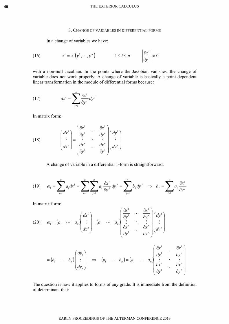
3. CHANGE OF VARIABLES IN DIFFERENTIAL FORMS

In a change of variables we have:

(16) nii yyxx ,,1 ni1 0j

i

yx

with a non-null Jacobian. In the points where the Jacobian vanishes, the change of variable does not work properly. A change of variable is basically a point-dependent linear transformation in the module of differential forms because:

(17)n

j

jj

ii dy

yxdx

1

In matrix form:

(18)n

nn

n

n dy

dy

yx

yx

yx

yx

dx

dx 1

11

1

1

1

1

A change of variable in a differential 1-form is straightforward:

(19)n

j

jj

n

i

n

i

n

j

jj

i

ii dybdyyxadxa

11 1 1

11

n

i

j

i

ij yxab

1

In matrix form:

(20)n

n

nn

n

nn

n

dy

dy

yx

yx

yx

yx

aadx

dxaa

1

1

1

1

1

1

1

11

n

n

dy

dybb

1

1

n

nn

n

nn

yx

yx

yx

yx

aabb

1

1

1

1

11

The question is how it applies to forms of any grade. It is immediate from the definition of determinant that:



(21) nn

nn

n

nn

n

n dydyyyxxdydy

yx

yx

yx

yx

dxdx 11

11

1

1

1

1

1

where the usual bridged notation for the Jacobian has been introduced. For forms of a grade less than the number n of variables involved in the change, the expression is intermediate between (18) and (21), but the entries of the matrix of change of basis are always Jacobians of an order equal to the grade of the differential forms. For instance:

(22) ll

jk

k

jl

l

i

kk

iji dy

yxdy

yxdy

yxdy

yxdxdx

lklk

jilk

l

j

k

j

l

i

k

i

lkk

j

l

i

l

j

k

i

dydyyyxxdydy

yx

yx

yx

yx

dydyyx

yx

yx

yx

where Einstein’s summation convention has been applied. In the same way:

(23)

nmlnml

kjinml

n

k

m

j

l

i

n

k

m

j

l

i

n

k

m

j

l

i

kji dydydyyyyxxxdydydy

yx

yx

yx

yx

yx

yx

yx

yx

yx

dxdxdx

and so on.

4. POINCARÉ LEMMA

A differential form is said to be closed if 0d , and exact if there exists another differential form such that d . As we have seen above, every exact differential form is closed. However, the question is to know under which conditions a closed differential form is exact. The answer is the Poincaré lemma: If nA is a star-shaped open set, then every closed differential form is locally exact [3, p. 40], [4, p.86]. An important fact is that the primitive of that the Poincaré lemma ensures to exist is not unique. That is, any other differential form of the kind d is also a primitive of :



(24) 'dd'

d

5. PRIMITIVES OF CLOSED DIFFERENTIAL FORMS

Laurent Schwartz [5] provided an iterative method to calculate a primitive 1 of an exact differential form . Let us suppose that is a linear function of exterior products of ndxdx ,1 . Then, we can write as:

(25) 111 MLdx

where 1L and 1M are uniquely defined by the requirement that they do not contain 1dx .

Now we calculate a differential form 1 such that 1

11 x

L through the integration of

1L from 0 to 1x keeping nxx ,2 constant. When subtracting the differential of 1

from , one obtains a differential form not containing 1dx and not dependent on 1x . If the subtraction yields zero we have finished. If the subtraction yields a differential form, we repeat the process by separating those terms containing any of the surviving idx ,which we assume to be 2dx , from those not containing it:

(26) 2221 MLdxd

where 2L and 2M only contain exterior products of ndxdx ,3 and do not depend on

1x . In order to obtain 2 , one integrates 2L from 0 to 2x keeping nxx ,3 constant. Subtraction of 2d from 1d yields another differential form only containing exterior products of ndxdx ,3 , and so on until exhausting :

(27) 021 kddd nk

When this subtraction equals to zero, we have found a primitive k211 . Then, the indefinite integral will be d1 , where

is a differential form whose grade is a unit lower than the grade of because 02d .d plays the same role as the constant of integration in the differential calculus of one variable.

Let us apply, for instance, Schwartz’s method to the differential form (28), which is closed because 0d , According to the Poincaré lemma a local primitiveexists such that d . Let us write in the form of equation (25):

(28) dxdzzxdzdyyxdydxzyx 2222

dzdyyxdzzxdyzyxdx 2222



By integration of L from 0 to x we find :

(29) dzzxdyzyxdzdzdydzyLd

xxx

22

222

00

2

0

whose differential is:

(30) dxdzzxdzdyyxdydxzyxd 2222

Notice that dx must be placed on the left of the exterior product of differentials in (29), which has implied a change of sign of the second integral. Integration is the inverse operation of exterior differentiation (3), so that the differential of the variable with respect to which the integration is carried out must be placed on the left like in (3). We now see that d and (30) is therefore a primitive. If 0d we would repeat the process for dy . The indefinite integral of will be:

(31) dzzxzfdy

yfzyxdx

xf

2

222

For instance, for 8

22 zxf we find another primitive 2 :

(32) dzzxdyzyxdxzx44

222

2

2

Another example is provided in the integration of the differential form (45).

6. DEFINITE INTEGRALS OF DIFFERENTIAL FORMS

A differential form that is not exact can nevertheless be integrated in the sense that follows. The definite integral so obtained will depend on the manifold where the integration is carried out. Let us see, for instance, a line integral, the integral of a differential 1-form, following two distinct paths 1L and 2L between two given points:

(33)

1,1,1

0,0,0

2 dzyzdyyxdxx

L

If we follow the path tttzyxL ,,,,1 we have:



(34)372

34

1

0

23

1

0

2

1

ttdttt

L

But, if we follow the path 322 ,,,, tttzyxL we have:

(35)47

423

1

0

423

1

0

32

2

tttdtttt

L

The results of both integrations differ because the differential form is not exact:

(36) dzyzdyyxdxx 2 0dzdydydxd

7. STOKES’ THEOREM

Stokes’ theorem states that if is a smooth differential (k-1)-form with compact support on a smooth manifold D of dimension k with boundary D then it satisfies:

(37)

DD

d 1kx kDdim

7.1 Case 1k : line integrals. When it applies to exact differential 1-forms, line integrals can be computed in a very easy way:

(38) AfBfdzzfdy

yfdx

xf

BAL

where BAL is any path. In vectorial notation:

(39) AfBfdlf

BAL

grad

where dl is the line element:

(40) 321 edzedyedxdl

and the gradient operator is:

(41) 321grad ezfe

yfe

xff



Going to a concrete example, let us consider the line integral:

(44)

1,0,1

0,1,0

22

1,0,1

0,1,0

2122 dzxyxdyzxdxzxyz

Let us check that the differential 1-form is closed:

(45) 02122 22 dzxyxdyzxdxzxyzdd

According to the Poincaré lemma, has a primitive to be obtained by Schwartz’s method. By integrating from 0 to x we have:

(46) xzyzxdxzzy

x

222 2

0

1

dzxyxdyzxdxzxyzd 222 221

dyd 1 y2

021 dd

(47) Cyxzyzx 2221

(48) 1122 1,0,10,1,0

2

1,0,1

0,1,0

yxzyzx

As an alternative, try to integrate the line integral (48) for a path given by tttzyx 2sin,cos,sin,, . Then the line integral becomes:

(49)

2/

0

5223

1,0,1

0,1,0

sinsincossin4cossin4 dttttttt

The computations that follow take much more time.

7.2 Case 2k . Surface integrals. In this case Stokes’ theorem relates surface integrals to line integrals along the boundary of the integration surface. For the concrete case of the plane, we have Green’s theorem:



(50)

DLD

dyqdxpdydxyp

xq

where D is a closed region in the plane and L is the curve that bounds D . The line integral on the right must be taken with a counterclockwise orientation. An elemental proof of Green’s theorem can be found in handbooks such as [6, p.440].Following the case 2k for the three-dimensional space, we have Stokes’ original theorem:

(51) dxdzxr

zpdzdy

zq

yrdydx

yp

xq

dzrdyqdxp

where is a region with boundary in a surface of the three-dimensional space, and is the closed curve that bounds . In this way, the components of the curl of the vector field rqpv ,, are:

(52) yp

xq

xr

zp

zq

yrv ,,curl

7.3 Case 3k . Gauss’ theorem. If Stokes’ general theorem is applied to differential 3-forms in the space we have Gauss’ theorem:

(53)

VV

dydxrdxdzqdzdypdzdydxzr

yq

xp

which relates a volume integral in a volume V with a surface integral over the closed surface V that bounds the volume V . In this way, the divergence of a vector field rqpw ,, is:

(54) zr

yq

xpwdiv

8. THE DIFFERENTIAL OPERATORS IN ORTHOGONAL CURVILINEAR COORDINATES

Another application of exterior differential is the deduction of expressions for the differential operators gradient, curl and divergence. The line element dl in curvilinear orthogonal coordinates of the three-dimensional space is:



(55) 33

322

211

1 eduheduheduhdl 12ie 0ji ee if ji

where ih are called scale factors. Locally, we can always write the line element as an Euclidean line element [7, p. 95]:

(56) 33

22

11 eeedl i

ii duh

The differential of a function f is:

(57) 33

22

11 du

ufdu

ufdu

ufdf

which can be written in the local Euclidean basis:

(58) 33

3

22

2

11

1

111uf

huf

huf

hdf

The components in the basis i are called physical components because they are the components that a local observer would see. The vector having the physical components of the differential of a function (58) is the gradient operator [8, p. 250], [9, p. 269]:

(59) 33

22

11

1,1,1graduf

huf

huf

hf

In the same way, the differential 1-form of a vector field1321 ,, aaaA is:

(60) 333

222

111

33

22

11 duahduahduahaaa

The differentiation of this 1-form yields a 2-form:

(61) 323

222

33212

111

22 duduuah

uah

duduu

ahuahd

131

333

11 duduuah

uah

which can be written in the local Euclidean basis i (56) as:

(62) 131

333

11

31

323

222

33

32

11uah

uah

hhuah

uah

hhd

1 Here, the vector field A is a polar vector such as linear momentum or the electric field, which changes the sign under the inversion of coordinates.



212

111

22

21

1u

ahuah

hh

Then, the physical components of the curl are [8, p.250], [9, p. 275]:

(63) ,1,1,,curl 322

233

322

111

22

21321 u

ahu

ahhhu

ahuah

hhaaa

133

311

13

1uah

uah

hh

Let us consider the differential 2-form associated to a vector field2

321 ,, bbbB :

(64) 213132321 bbb

21321

13213

32132 dudubhhdudubhhdudubhh

After differentiation we find:

(65) 3213

3212

2131

132 dududuu

bhhu

bhhu

bhhd

and by writing the result in the local Euclidean basis:

(66) 3213

3212

2131

132

321

1u

bhhu

bhhu

bhhhhh

d

the divergence operator [7, p. 77], [8, p. 250], [9, p. 272] is obtained:

(67) 3321

2213

1132

321

1divu

bhhu

bhhu

bhhhhh

B

9. APPLICATION OF THE FORMULAS OF DIFFERENTIAL OPERATORS TO ELECTROMAGNETISM

Let us apply the differential operators to electromagnetism. For instance, the electric field E is obtained from the vector potential A and the scalar potential as:

(68)tAE grad

2 Here, the vector field B is an axial vector such as angular momentum or the magnetic field, which remain invariant under the inversion of coordinates.



On the other hand, the magnetic field B is obtained from Lorentz’s equation:

(69) AB curl

The expressions for gradient (59) and curl (63) can be applied to equations (68) and (69) because E is a polar vector and B an axial vector. Maxwell’s equations in the vacuum are:

(70) (a) tBEcurl (b) 0divB

(71) (a) 0

divE (b) tE

cjB 20

1curl

where is the electric charge density, j is the electric current density, c is the speed of light in the vacuum, 0 is the vacuum electric permittivity and 0 the vacuum magnetic permeability. There is a fundamental difference between eqns. (70) and (71). In (70a) the curl is applied to a polar vector yielding an axial vector so that the expression (63) for curl holds. In (70b) the divergence is applied to an axial vector and therefore the expression (67) for divergence is also valid. However, in (71) (a) the divergence is applied to a polar vector, which is not the exterior differentiation of (64), and in (71 b) the curl is applied to an axial vector, which is not the exterior differentiation of (60). Then the formulas (63) and (67) cannot be applied (although this happens currently) to eqns. (71). In order to have a wider view of the insufficiency of the exterior differential, let us see Maxwell’s equations in the space-time. The electromagnetic field F has grade 2 [10, 11] and corresponds to the differential 2-form [12]:

(72) dydxBdxdzBdzdyBdtdzEdtdyEdtdxEF zyxzyx

The vector potential A is a differential 1-form:

(73) dtdzAdyAdxAA zyx

Equations (68) and (69) are included in the exterior differentiation:

(74) FdA

Obviously, a second exterior differentiation yields zero:

(75) 02 AddF

which accounts for Maxwell’s equations (70), but not for (71). Clearly, Kähler differentiation is needed if we want to get the current density and the charge by differentiation of the electromagnetic field F. Firstly, we can write instead of (74):

(76) FAd



which yields additionally the Lorentz normalization condition:

(77) 012 tcz

Ay

Ax

AAd zyx

Here we have applied Kähler’s signature (3,1), that is, 1222 dzdydx and 122dtc for lengths measured in meters and time in seconds. In a second step we can

write instead of (75):

(78) JkFdFd

where J is the current density vector of the special relativity:

(79) dzdydxdtdydxjdtdxdzjdtdzdyjJ zyx

whence we deduce that the constant k is a pseudoscalar, because Fd is a differential 1-form:

(80) dtdzdydxk0

1

Equations (76) and (78) yield d’Alembert’s equation:

(81) JktA

cAAdd 2

2

2

1

where 2

2

2

2

2

2

zyx is the Laplacian. The inner differentiation of (81) results in

the equation of continuity:

(82) Jkdt

Adc

AdtA

cAd 2

2

22

2

2

11

because the d’Alembertian commutes with the inner differentiation. Now, taking into consideration the Lorentz normalization condition 0Ad (77), we finally arrive at the continuity equation:

(83) 00tz

jyj

xj

kJd zyx

Therefore, the Kähler calculus provides a full description of electromagnetism, from potentials to currents, which cannot be given by the exterior calculus.



REFERENCES

[1] É. Cartan, «Sur certains expressions différentielles et le problème de Pfaff», Ann.École Norm. 16 (1899) 239-332.[2] É. Cartan, Les systèmes différentiels extérieurs et leurs applications géométriques. [3] H. Cartan, Formas diferenciales, ed. Omega (Barcelona, 1972). Translation into Spanish of Formes différentielles: applications élémentaires au calcul des variations et à la théorie des courbes et des surfaces, Hermann (Paris, 1967), also translated into English in Differential Forms (Dover, 2006). [4] M. Spivak, Cálculo en variedades, ed. Reverté (Barcelona, 1982). Translation into Spanish of Calculus on Manifolds, W. A. Benjamin Inc. (N.Y.). [5] Laurent Schwartz, Analyse IV, collection Enseignement des Sciences, Hermann (Paris, 1993) p. 285. [6] E. Kreyszig, Advanced Engineering Mathematics, 9th ed., Wiley (Singapore, 2006). [7] J. G. Vargas, Differential Geometry for Physicists and Mathematicians. Moving frames and Differential Forms: From Euclid Past Riemann, World Scientific (Singapore, 2014). [8] L. Råde, B. Westergren, Mathematics Handbook for Science and Engineering, 5th

ed., Springer (Berlin, 2004). [9] J. J. Scala, Análisis Vectorial II, Funciones vectoriales y teoría de campos, ed. Síntesis (Madrid, 1998). [10] P. Lounesto, Clifford Algebras and Spinors, Cambridge Univ. Press (1997) p. 109. [11] R. González, El álgebra geométrica del espacio y tiempo (2011-) p. 33, available at http://www.xtec.cat/~rgonzal1/espacio.htm.[12] J. G. Vargas, Notes on Kähler Calculus (2016) p. 57, available at http://cs.unitbv.ro/~acami/noteskc.htm, also included in these Early Proceedings of the Alterman Conference 2016 (eq. 2.20 of chapter 4).



58


Summer School, phases 2, 3:

Kähler Calculus

and its Applications

José G. Vargas

Notes on the Kähler calculus for the Summer School

1. Perspective on the Kähler calculus

2. Kähler algebra

3. Kähler differentiations

4. Relativistic Quantum Mechanics

5. Lie differentiation and angular momentum

6. Conservation in Quantum Mechanics. Beyond Hodge’s theorem

59


60


Notes on the Kahler Calculus forthe Summer School

Jose G. Vargas

1 CHAPTER 1: Perspective on the Kahler Calcu-lus for Experts on Clifford Analysis

1.1 Reconsidered Program of the Kahler part ofthe summer school

This is the first of a few chapters that I plan to post in this web sitefor potential participants in the Summer School, phases II and III. Itprovides an illustration for (mainly) Clifford mathematicians who wouldlike to know what the Kahler calculus is about and what it offers. Start-ing with the second chapter, these notes will be used at the school forthe actual teaching.

For the moment, the table of contents will not be removed, so thatthe change will be easier to appreciate. I have come to the conclusionthat rather than teaching as much theory as needed for its multipleapplications, I shall present some materials and produce immediatelyapplications of it. Very occasionally I shall borrow a theorem (like auniqueness theorem) to be proved in a future chapter. The chaptersto be posted here will be only part of what will be lectured in Brasov,just enough to provide the flavor of it. Those who are in a positionto understand these notes and plan to attend the conference might beable to start reading the pertinent Kahler papers on their own and ask,during the lectures, questions more profound that they might be askingotherwise.

As an example, the second chapter will deal with Kahler algebra ofscalar-valued differential forms. It will be followed by a pair of applica-tions: the theorem of residues and, unrelated to that, a new perspective

1

61


on the issue of superposition, a concept to be replaced with decompo-sition, since it is through decomposition that the objects that one triesto superimpose are actually generated. Let me be more explicit. If thewave function is a member of the Kahler algebra, it can be written asa sum of pieces that belong to the ideals and also are solutions, butthis is not sufficient to make them particle states. If you start withparticle states (even mixing particles with antiparticles both with bothoptions for handness) you do not get that intermediate state where youdecompose but do not quite get particles, as one still needs somethingelse for this. Of course, one can introduce concepts like matrix densitiesor something of the sort to deal with issues of this kind. But this isnot as natural, or as rich or as reliable as starting with a solution of awave equation that you decompose to get spinors which are not yet wavefunctions for leptons living in the same ideals.

The third chapter will deal with, among other topics, Kahler differen-tiation of scalar-valued differential forms, strict harmonic and harmonicdifferentials, Dirac type spinors (before we even consider a Dirac typeKahler equation, since their form has to do with theory of solutions withsymmetry of exterior systems regardless of specifics), and so on. Appli-cations: Real complex-like calculus in the plane, Helmholtz theorem fordifferential 1−forms and 2−forms in 3-D Euclidean space, and a hint atwhy there is room for theory on quantum collapse of the wave functionand quantum teleportation in this calculus. These issues are intimatelyrelated to the issue of decomposition. One could say that these topicsare aspects of the same theory, which grows in sophistication as we keepbuilding more basic theory.

A fourth chapter will deal with the “Kahler-Dirac equation”, or sim-ply Kahler equation. A variety of applications for relativistic quan-tum mechanics follows: emergence of momentum operators, Pauli-Diracequation for particles and antiparticles, post Pauli-Dirac Hamiltonianand an additional couple of topics.

At about this point, we shall have reached the third phase of the Sum-mer School. It will deal with symmetry and conservation, a uniquenesstheorem for differential forms, integration at different levels of generalityfor differentials whose exterior derivative and co-derivative are known,Lie and Killing operators, unified spin and orbital angular momentum,total argument momentum and its square, antiparticles, leptons andquarks.

1.2 Introduction

The Kahler calculus is a calculus of tensor-valued differential forms. So,we have a product of structures. The restriction of the Kahler calculus

2

PERSPECTIVE ON THE KÄHLER CALCULUS

62


(KC) to scalar-valued differential forms is the generalization of the exte-rior calculus that results from replacing the underlying exterior algebrawith Clifford algebra. Clifford analysts are used to the replacement ofexterior with Clifford. Then, what is special here?

In the KC, the interior derivative of a scalar-valued differential 1−formis like the divergence, and the same derivative of a vector field is zero,not the divergence, as we shall see. That is such an obvious differencethat one can understand it before learning the KC. This difference hasits origin in the fact that there is a greater variety of elements in thefull Kahler calculus than in other calculi. But the real important dif-ferences consist in what the KC can do and the Dirac calculus cannot.Of course, this chapter is an exception. It is meant to provide a per-spective to those who can understand it. Everybody else should startwith the next chapter. So, if upon reading this chapter you start not tounderstand, abandon it and go to the next one. Just before moving tothe next chapter, please read the last four sections of the present one. Ihave given the exact places where the claims were proved by Kahler.

The files I may put in the web site of this summer school will bereferred as chapters because they will be so, up to minor modificationsin a book I am writing about what I shall call the Cartan-Kahler calculus.It was announced in my previous book “Differential Forms for Physicistsand Mathematicians”. I know some readers are looking forward to readit. There will be prior chapters on Clifford algebra and the exteriorcalculus. But, for the purposes of the summer school, this will be chapterone.

An outstanding feature of the KC is the ease with which one gets deepinto the world of quantum mechanics, immediately acquiring new vistassince one enters if through a different door. So much so that we shallspeak of the quantum mechanics, ab initio relativistic, that emerges as avirtual concomitant of the KC. At the end of this chapter, we shall brieflyillustrate some deep results for quantum mechanics that Dirac’s theorydoes not match. For the moment let us just say that the wave functionin the “Kahler-Dirac” equation for scalar-valued differential forms is formembers of the algebra in general, not only specifically for spinors (i.e.for members of ideals in this algebra).

Of course, there will be a lot of work to be done to revisit every pieceof physics from the new perspective. Better yet, just a little bit of Kahleralgebra will allow us, at the end of the next chapter, to start seeing howold problems can be seen in a new light. For the moment, I shall dealonly with some computational issues to respond to the question, whatis new?

3


63


1.3 Kahler and Cartan-Kahler calculi

As I mentioned in the second half of the biographical note of this website, the KC was formulated in three papers. The translation of the titleof the first of those papers is Interior and exterior differential calculus,and the translation of the third is The interior calculus. The author isdealing with the same calculus at the same level of generality. The onlymain difference is that the last of these two is far more comprehensivethan the first one. So, it appears that he was not too sure at some time(s)about what title he should have given to his calculus. The issue we havewith titles far transcends this one because of a far more important reason,as we are about to explain.

We are fully interested in Kahler’s calculus for scalar-valued differen-tial forms, not for tensor-valued differential forms, which we shall replacewith Clifford-valued ones. In the last two of these three cases, we aredealing with tensors products of algebras. Then, sometimes, we shallconsider a restriction to “mirror elements” (concept not needed at thispoint), which constitute a fourth structure. All four have to do withClifford structure but only one is a Clifford algebra. Hence, to minimizeclutter, I shall often use the term algebra not in the technical sense butin the more general sense of the dictionary, namely as a mathemati-cal system that uses symbols and specially letters to generalize certainarithmetical operations and relationships. In this wide sense, all four ofthose structures qualify as algebras.

Eventually, we shall use the terms Kahler’s algebra and KC to whenwe deal only with scalar-valued differential forms. When dealing withClifford valuedness, we shall use the terms Cartan-Clifford algebra andcalculus. It is worth noticing that Cartan considered curvatures as bi-vector valued differential 2-forms. We do not risk ignoring any applica-tions with tensor-valued differential forms, since Kahler did not produceany application for them.

1.4 Kahler’s differential forms

Kahler wrote his general differential forms as

uk1...kµi1...iλ

=1

p!ak1...kµi1...iλ l1...lp

dxl1 ∧ ... ∧ dxlp , (1)

where we are using Einstein’s convention of summation over repeatedindices. His excessive use of components is not a desirable feature fora calculus, but has a very useful consequence. It shows explicitly thatwe must consider two types of subscripts. They refer to two essentiallydifferent concepts: scalar-valued differential r-forms (quantities with justa l series of indices) and tensor-valued differential 0-forms or tensor fields

4


64


(quantities with only k and or i series of indices). Hence, his calculi areab initio different from all other known calculi that are based on Cliffordalgebra. But Kahler did not exhibit the basis elements that pertain tothe i and k indices.

The affine curvature is a very well known example of the rare quan-tities that have indices of all three types. Consider some vector-valueddifferential 1-form. It need not be closed. For simplicity let us assumethat it were what Cartan and Kaehler would call the exterior derivativeof a vector field, though practitioners might refer to it with the name ofcovariant derivative, name which is here reserved for a different purpose.We have

dv = dviei + vkdek = (dvi + vkωik)ei. (2)

Differentiating next dv, we obtain a vector-valued differential 2−form,ddv (which happens to be zero in Euclidean space), but we shall ig-nore this (you may assume that the manifold is only approximately aEuclidean space). The components of ddv are not what in the tensorcalculus one calls covariant derivatives. For that, we would have to dif-ferentiate vj;kφ

kej, where (φi) is the basis of covariant vector fields dual

to the basis field (ej), i.e. φi ek = δik. Let us not overlook that, in the

Kahler calculus, a differential 1−form is not a covariant vector (i.e. alinear function of vectors) field, but a function of curves, evaluated byintegration on a given curve.

We get five terms for ddv, two from the differentiation of dviei, andthree more from the differentiation of vkωi

kei. The first term, ddvi isobviously zero. The second and third terms cancel each other out. Wethus have

ddv = vkd(ωikei) = vk(dωi

k − ωjk ∧ ωi

j)ei. (3)

Since dωki − ωj

i ∧ ωkj is a differential 2−form, it is of the form. Hence,

ddv = viRki l1l2

ωl1 ∧ ωl2ek. (4)

This says that the components of the vector-valued differential 2−formddv are viRk

i l1l2. We then define curvatures by

≡ Rki l1l2

ωl1 ∧ ωl2φiek, (5)

where all three types of indices are involved. Clearly ddv results fromevaluating in v,

v =Rki l1l2

ωl1 ∧ ωl2φiek vmem = vk(dωik − ωj

k ∧ ωij)ei = ddv. (6)

For more on this approach to affine curvature and the use of bases ω ofdifferential 1−forms (which are of the essence further below), check in

5


65


your library my book “Differential geometry for physicists and mathe-maticians”. I do not know of any other book which stays close to thisCartanian way of doing modern differential geometry, or to the Kahlercalculus for that matter.

1.5 Kahler’s differentiation

In Kahler, all differentiations except Lie differentiation are based on hisconcept of covariant differential. He gives it ab initio as

dhak1...kµi1...iλ l1...lp

=∂

∂xhak1...kµi1...iλ l1...lp

+

+ Γk1hra

r...kµi1...iλ l1...lp

+ ...+ Γkµhra

k1...ri1...iλ l1...lp

− Γrhi1

ak1...kµr...iλ l1...lp

+ ...+ Γrhira

k1...kµi1...r l1...lp

− Γrhl1

ak1...kµi1...iλ r...lp

+ ...+ Γrhlra

k1...kµi1...iλ l1...rp

, (7)

where the gammas are the Christoffel symbols. Since this equation willprobably put many readers off, let me start by saying that the author ofthese notes does not keep anything like this in his memory, nor does helook for this formula when needed. There is a better way of doing hisdifferentiations. At this point, let me just make some helpful comments.

The differential of scalar-valued differential forms written in termsof Cartesian coordinates requires only the first of those four lines. Thatis good enough for many applications. If the differential form is scalar-valued but the coordinates are not Cartesian, dh involves only the firstand fourth lines, regardless of whether the metric is the Euclidean met-ric disguised by the use of an arbitrary coordinate system or whether itis a proper post-Euclidean Riemannian metric. Lines two and three arefor the non-scalar valuedness but only when the affine connection is theLevi-Civita (LC) connection. If the connection were another one, thosesymbols would have to be replaced with the components of the given(metric compatible) affine connection of the space. But the fourth linewould not change in this respect, as it does not depend on the connectionbut only on the metric and its derivatives through the Christoffel sym-bols. In addition to generalizing this formula for arbitrary connection,one could also replace the tensor-valuedness with Clifford valuedness.And let us not ignore either that vector-valuedness can take place inexterior algebra, Clifford algebra and tensor algebra contexts. It doesnot make a difference.

A more efficient, less cumbersome way to deal with “Kahler differen-tiation” resorts to inferring the specific form of the covariant derivativein each case from the equations of structure of the manifold. That iswhat we are about to do.

6


66


Let us give the basic ideas about Kahler differentiation, representedby the symbol ∂. We seek to find an operator ∂ such that ∂ ∨ u (=∂ ∧ u+ ∂ · u) will become

∂u = du+ δu, (8)

with ∂ ∧u = du, and such that δu will be intimately connected with the

divergence. In Cartesian coordinates, ∂ could be simply dxi ∂

∂xi. But this

is not good enough for general coordinates, as the form of the divergencein curvilinear coordinate attests to. For this reason, we shall rather seek∂u in the form

∂u = dxi ∨ diu. (9)

for some covariant derivatives diu canonically determined by the struc-ture of the manifold and such that dxi ∧ diu = du. The notation

∂u = ∂ ∨ u = ∂ ∧ u+ ∂ · ustill is justified if we understand it to mean

∂ ∧ u = dxi ∧ diu = du, ∂ · u = dxi · diu = δu.

We have just connected with the exterior calculus, which we are extend-ing with this δu, once we define diu. This will be much richer thanRicci, or de Rham or Dirac theory since the context is much larger thanin those theories. The proof will be in the pudding. We shall thus referto δu as the interior derivative since it is a concept more comprehensivethan divergence depending on what objects u the operator δ is appliedto.

1.6 Kahler’s differentiation through geometric struc-ture

Assuming we had already computed du by the standard formula in theexterior calculus, we might try to infer diu from du = dxi ∧ diu. Butdu does not determine di or ∂, which is the reason why we have notdisplayed dxi∂/∂i . It would work for the exterior derivative. but itwould not yield the right divergence. But there is one such solutionthat is canonically determined by the equations of the structure of themanifold endowed with a metric, regardless of whether the manifold hasan affine structure or not.

Define a set of n differential forms ωi’s such that

ds2 =n∑

i=1

(ωi)2, (10)

7


67


for any specifically given quadratic symmetric differential form ds2 =gijdx

idxj (i = i, ..., n). These ωi are defined up to the most generalrotations in dimension n.

As any good book on differential geometry shows, the system ofequations

dωi = ωj ∧ ωij, ωij + ωji = 0 (11)

defines a set of ωij’s. For the same metric, we may consider the system

0 = d(dxi) = ωj ∧ αij, dhgkl = 0,

the second of these equations being known as the statement that thecovariant derivatives the metric is zero. The Christoffel symbols aredefined by αi

j = Γijldx

l.The last two systems define the same mathematical object. This

does not mean that the αij and the ωi

j are equal, or even the componentsof some object of grade two. The Γi

jl and the Γ′ijl defined by ωi

j = Γijlω

l

are related by non-tensorial equations known as the transformations ofconnections. The mathematical object of which the αi

j’s and the ωij’s

are components is a differential form valued in the Lie algebra of theEuclidean group (actually of the affine extension of the Lie algebra ofthe Euclidean group; do not bother about these details) of dimension n.All those other differential forms are components. It is legal tender nev-ertheless to call them differential forms by making them so as a matterof definition. I shall try to explain this with what should amount to asimpler example.

The first element of orthonormal vector bases at some point of Eu-clidean space is not a vector, but a set of them: cosφ i − sinφ j. It isbasis dependent. Once a basis has been chosen, say for φ = π/4, wehave a vector (2)−1/2 i −(2)−1/2 j. We can now take this vector and ex-press it in terms of any other basis (in particular for φ = π/3), whereit is not its first element. This type of idea is involved at a far moresophisticated level in the difference between αi

j and the ωij. For a deep

understanding of this, see my book “Differential geometry for physicistsand mathematicians” if you do not know of any other book dealing withthis subject (I do not any, except for information scattered over a vari-ety of E. Cartan’s papers). The book is now in 500 libraries, hopefullyenough of them to have one in a library of your country, where institutioncould get it for you if it does not have it.

In order to do differentiation in terms of bases that are not coordinatebases, we first define f/k as given by df = f/kdx

k. We then have

dv = ai/jωj ∧ ωi + al ∧ dωl = ωj ∧ ai/jω

i + alωi ∧ ω l

i =

= ωj ∧ ai/jωi − alΓ

li jω

j ∧ ωi = ωj ∧ (ai/jωi − alΓ

li jω

i). (12)

8


68


By virtue of the relation of this formula to the structure of a manifold,it pertains to define Kahler’s covariant derivative djv of a differential1−form v = aiω

i asdjv = ai/jω

i − alΓli jω

i (13)

If ωi is dxi, the covariant derivative djv becomes

djv = ai,j dxi − alΓ

lijdx

i. (14)

For rectilinear coordinates, thus Cartesian in particular, dj reduces tothe partial derivative with respect to xj since the Christoffel symbolsthen become zero. For the interior derivative, we then have

δv = dxj · djv = dxj · dxi(ai,j −alΓlij) = gij(ai,j −alΓ

lij) = aj,j −alΓ

jlj.

(15)We have not written δv as ∂ · v since dj now is ∂j − lΓ

jlj . We use the

underbar because a has different subscripts on the two terms of djv.Let us return to dωi = ωj ∧ αi

j. For differential 1−forms dxj, theexterior derivative, d(dxi), is zero, and so is dxj∧αi

j. On the other hand,the connection equations are

dei = −ωije

j, (16)

from which we would infer dhei, and similarly for dhei. The comput-

ing of interior and Kahler derivatives will be easily achieved from theseequations. It is really simple.

1.7 Perspective on two physical applications devel-oped by Kahler himself

This preview for Clifford analyst would be only one half of an importantpicture without mentioning a couple of very important physical implica-tions of the quantum mechanics that appears to spring out of it, withoutobvious alternative. Both of them are related to the fact that, unlikeDirac’s theory, Kahler’s quantum mechanics is not about spinors butabout differential forms. Spinors, in the form of members of ideals ofthe Kahler algebra, are a concomitant of the treatment of solutions withsymmetry of exterior systems, as any system of differential equationscan be shown to be.

In his 1960 paper, Kahler starts with a profound treatment of partialdifferentiation of differential forms with respect to the angular coordinateassociated with rotational symmetry. Eventually, both spin and angularmomentum emerge from it, at par. Tracing spin from the end of Kahler’sderivation to the beginning of his argument, we realize that spin startsits life in Kahler ’s theory inside a partial derivative of a field conceived

9


69


not as a probability amplitude, but as a more conventional type of field;not as a spinor or member of an ideal in the algebra, but as a memberof the algebra itself independently of any ideals.

In addition to the elegance and reliability of Kahler’s argument, thisreading in reverse shows that a particle is “some special part of the field”,not just something that mediates among the particles, since these aresimply special configurations of it. This is consistent with Einstein’sview, though not exactly, as expressed by his words in correspondencewith Einstein: “To realize the essential point of atomistic theory, it issufficient to have a field of high intensity in a spatially small region ...”.This idea of Einsteinean pedigree finds natural implementation in theKahler calculus.

As profound as this result is in connection with spin, there is anotherone as profound, namely the treatment of not charge, not antiparticles,not energy, but all three at the same time. Let me give an inkling ofwhy this is so. A solution with time translation symmetry of a quantumequation is known to require a phase factor with time and energy inthe exponent. But, if the equation is written as an exterior system (asin the Cartan-Kahler theory of systems of differential equations), onealso needs as factors two idempotents that define complementary ideals.Each of these belong to the signs of charge for each value of the energyin the phase factor.

Why may we make such a statement about charge? Kahler alreadyexplained why. It is a consequence of the decomposition into two termsof the wave function of a Kahler-Dirac equation under time translationsymmetry, one from each of two complementary ideals. The correspond-ing conservation law for the wave function is then composed of two parts,one for each of those two terms. The left hand side of this law becomesthe sum of the left hand sides of two conservation laws, not the sum oftwo conservation laws. The small difference between the two pairs ofsimilar terms emerging in the process led Kahler to identify a physicalmagnitude, the electromagnetic charge, which may have two signs. Thesame energy but two signs of something when the coupling is electromag-netic coupling led him to view the two terms as representing particle andantiparticle. There is no need for an infinite sea of negative energy solu-tions, the weirdness of this concept being kept virtually silent in modernquantum physics. If Kahler had done his work in the late 1920’s, wewould be asking in 2016: ”Dirac who?” Of course, Dirac was a geniussince he provided a solution, though imperfect, to a problem for whichthe mathematics was not yet ripe.

10


70


CHAPTER 2: Kahler Algebra

Jose G. Vargas

Participants in this summer school will at this point know enoughClifford algebra not to be confused if we sometimes represent Cliffordproducts with the inverted wedge product sign and at other times byjuxtaposition.

The Kahler calculus is a little bit strange. This may be becauseit is an approximation to something much deeper and to which I shallrefer as the Cartan-Kahler calculus and which reconciles the ways ofCartan in differential geometry with the ways of Kahler on matters ofcalculus. One gets the impression that Kahler did not totally absorbCartan’s teachings in differential geometry. For this reason we shall usethe term Kahler geometry and calculus when dealing only with scalar-valued differential forms. This less comprehensive version is enough toproduce a great simplification of proofs and mathematical argumentswhen compare with the same issues in the standard mathematical andphysical paradigms.

1 A practical approach to Kahler algebra

Hervibores in the African savanna are born knowing how to walk andsoon learn how to run. They must have acquired some concept of runningby the time one of them spots a lion and sends a signal to the herd andeverybody starts to run. Of course, they do not know the anatomy andphysiology involved in running but they surely know how to run. I donot need to explain how this example applies to this section. Thus,after reading section 1, one can jump to section 3 of this chapter andproceed with the integrations that are usual in an undergraduate coursein complex variable. But, for the developments in the next chapters,one will have to read sections 1, 2 and 4. Readers who may not like theKahler calculus are invited to develop alternatives that will efficientlymatch Kahler’s results.

11

71


1.1 Definition of basic products

Kahler algebra (of scalar-valued differential forms) on a differentiablemanifold (not on a tangent space or cotangent space!!!) endowed with ametric is the Clifford algebra defined by the relation

dxidxj + dxjdxi = 2gij. (1)

Hence

dxi∧dxj+dxj∧dxi = 0, dxi ·dxj = gij =1

2(dxidxj+dxjdxi), (2)

which come together as

dxidxj = dxi ∧ dxj + dxi · dxj. (3)

If the differentiable manifold is a Euclidean vector space and the coordi-nates are Cartesian, we simply replace gij with δij. All this can be saidin a very elegant manner without using bases, but the definition wouldbe very abstract. We have said emphasized the “of scalar-valued differ-ential forms” to make sure we avoid confusions. Kahler also considereda more general structure consisting of tensor-valued differential forms.These do not constitute a Clifford algebra but the tensor product of atensor algebra by the Kahler algebra just defined.

Let (A,B) be an ordered pair of two points in a differentiable mani-fold. Let γ be any curve with ends at those points. By definition dxi isthe function of curves such that∫

γ

dxi = xiB − xi

A. (4)

Notice that we have not invoked either linear functions (i.e. covariantvectors) or covariant vector fields.

Consider next the differential form 3dx+xdy on curves between thosesame points. The integration depends on curves since this differentialform does not have a potential function. Finally compute (To avoidconfusion, I did not say evaluate) 3dx+xdy at any point with coordinatex equal to 2. We obtain 3dx + 2dy. This is not something that we canevaluate on γ because it is not legal to first compute it at a point andthen evaluate it on a curve, unless the differential form to be evaluatedhad been defined as 3dx+2dy in the first place. The most we can do inthis respect is to associate with 3dx + xdy equal to 2 points the linearfunction of tangent vectors 3φ1 + 2φ2 where φi ai = 1, φi aj = 0 fori = j.

12

KÄHLER ALGEBRA

72


The pair (A,B) is the boundary of the manifold γ. So, Eq. (4)is a particular case of Stokes generalized theorem, which is here usedas a definition, the reversion of roles of theorems and definitions beingpermissible. The formula for the exterior derivative would be a theoremrather than a definition. This may not be the most expedient course ofaction for the development of a calculus, but it is the most fundamentalsince integration requires less restrictive conditions than differentiation.Notice that we have not given any rule about differentiation yet, sincenone was needed.

One would proceed in similar manner for differential r−forms, i.e.as functions of r−surfaces. The use of Stokes theorem as a definitionis nothing new. Elie Cartan already used it almost a century ago fordefining the exterior derivative of a differential form whose coefficientsare not differentiable functions.

Although we should not care too much at this point about the sig-nificance of the dot product of two differential 1−forms, let us make afew remarks that may be helpful and a preview of arguments to come.In Cartesian coordinates, products dxi · dxj are zero unless i = j. Butdxi · dxi does not have an invariant meaning;

∑n1 dxi · dxi does. One

would then have to see these products in context.∑n

1 dxi · dxi. Thisexpression is related to some beautiful canonical Kaluza-Klein geometrywhich supersedes standard differential geometry. Again, we shall have towait for Cartan-Kahler calculus in order to go deeper into it in a futurechapter. Without going into any of that and not even raising the issue,Kahler obtained great results with the structure just mentioned. Theyeliminate significant problems of standard quantum mechanics.

Kahler used bases of differentials of arbitrary systems of coordinates,Cartesian coordinates not existing in non-Euclidean or non-pseudo-Euclideanspaces. Hence, we would have

dxidxj + dxjdxi = 2δij. (5)

in the Cartesian case. We would have to also replace gij with δij in (2).We prefer to use bases (ωl) constituted by linear combinations of the

differentials of the coordinates, whether these are Cartesian or not. Weshall again have

ωiωj + ωjωi = 2gij (6)

But we can always orthonormalize the metric so that we get

ωiωj + ωjωi = 2δij, (7)

regardless of whether the manifold is a Euclidean space or not.

13

KÄHLER ALGEBRA

73


The ωi notation is common in differential geometry developed withdifferential forms, usually in context of theory of connections. But thisnotation has nothing to do with connections, just with the metric. Ofcourse, one can get Christoffel symbols and the Levi-Civita connectionfrom the metric and its derivatives, but they are not needed at all forpresent purposes.

Let ωi be defined by ωj · ωi = δji for all pairs of indices. The ωi’sare not meant to be linear functions on the module spanned by the basis(ωj) (The concept of module is more general than that of vector space,but you will not have problems here if you think of a module as if it werea vector space). Nothing could be more misleading than to think of theωi’s as linear functions of anything. They are specific cases of functionsof curves, just as legitimate as the ωi’s. They constitute just alternativebases in the module of differential forms.

Kahler likes to define the symbol ei where we use the left dot multi-plication “ωi·”. The action of ei has the distributive property since, aswe know,

ωi·(ωj∧ωl∧ωk) = (ωi·ωj)(ωl∧ωk)−(ωi·ωl)(ωj∧ωk)+(ωi·ωk)(ωi∧ωj. (8)

And similarly for “ωi·(ωj∧ωl∧ωk)”, since ωi is as legitimate a differential1−form as ωi. We thus have

ωi·(ωj∧ωl∧ωk) = (ωi·ωj)(ωl∧ωk)−(ωi·ωl)(ωj∧ωk)+(ωi·ωk)(ωi∧ωj (9)

or, equivalently,

ei(ωj∧ωl∧ωk) = (eiω

j)(ωl∧ωk)−(eiωl)(ωj∧ωk)+(eiω

k)(ωi∧ωj. (10)

Some learned readers would prefer to base the calculus and evendifferential geometry on vector field equations that largely parallel thosewe have given. A participant in this summer school already did so. Theadvantage of the Kahler way is that he deserves vector fields for otherpurposes. The parallelism ceases as soon as we consider differentiation.In any case and for the moment, I am reproducing what Kahler didand shall later show my view of where one should go, guided by theapplications that ensue from the course of action to be followed. At thispoint I advocate the Kahler course of action because of the results heobtained and which nobody else appears to have even matched.

1.2 Using D=2 to get used to Kahler algebra

In terms of polar coordinates in 2-D Euclidean space E2, we have

((dρ)2 = 1, (dφ)2 = dφ · dφ =1

ρ2, dρ · dφ = 0. (11)

14

KÄHLER ALGEBRA

74


dxdy = −dydx, (dxdy)2 = −1. (12)

We use the abbreviation i for dxdy. The complex-like inhomogeneousdifferential form z,

z.= x+ ydxdy

.= x+ yi, (13)

emerges from the relation between (dρ, dφ) and (dx, dy):

dφ =xdy − ydx

x2 + y2=

x− ydxdy

x2 + y2dy =

1

x+ ydxdydy = z−1dy, (14)

dρ =xdx+ ydy

(x2 + y2)1/2= ρ

x− ydxdy

x2 + y2dx =

ρ

x+ ydxdydx = ρz−1dx. (15)

By virtue of (13), it is clear that

z±m = (x+ yi)±m = ρ±memφi = ρ±m(cosmφ± i sinmφ), (16)

for integer m.There is a laudable effort on the part of Clifford mathematicians to

replace the imaginary unit with elements of real Clifford algebra, aneffort with which this author wholly agrees. But I see that there hasbeen an abuse of the replacement of the imaginary unit with the unitpseudo scalar of the algebra when some other element in the algebra ofsquare minus one is a more natural choice. So, rather than replace, itis a better process to let the right element emerge without resort to areplacement, which is what we have done in this case and shall be doingtime and time again. And nothing impedes to proceed in reverse, andabbreviate (once found) dxdy as i, and write cosmφ ± dxdy sinmφ aseimφ. e shall sometimes use dxdy and i simultaneously, choosing one orthe other in each specific case depending on what we wish to emphasizeFinally, here is a remark for those without much Clifford experience whomay have read this paragraph. The square of the unit pseudo-scalar maybe plus or minus one. It depends on dimension and signature.

Let α be a differential 1−form and let u and v be scalar functions.We have

(u+ vi)α = α(u+ vi)∗, (17)

where(u+ vi)∗ ≡ u− vi, (18)

and, in particular,

z∗ = x− yi, z∗ = ρ2z−1 (z∗)−1 = ρ−2z, (19)

with i = dxdy. Clearly

u =(u+ vi) + (u+ vi)∗

2, v =

(u+ vi)− (u+ vi)∗

2i, (20)

as in the calculus of complex variable but again with i = dxdy.

15

KÄHLER ALGEBRA

75


1.3 The angular integrand

For the purpose of certain integrations,we wish to have the angular inte-grand part j(ρ, φ)dφ of a differential 1−form α = h(ρ, φ)dρ+ j(ρ, φ)dφ,when it is given in terms of Cartesian coordinates

α = k(x, y)dx+ g(x, y)dy. (21)

We clearly havej = ρ2 α · dφ (22)

and, therefore,

α = wdx, w ≡ k − gdxdy = k − gidy. (23)

We proceed to compute j. For that purpose, we express the dot prod-uct in terms of Clifford products:

j = ρ2(wdx) · (z−1dy) =ρ2

2

[wdxz−1dy + z−1dywdx

]=

=ρ2

2

[w(z∗)−1i− z−1w∗i

]=

1

2[wz − w∗z∗] i = −(wz)(2), (24)

where the superscript refers to the coefficient of the differential 2−formpart (of wz in this case). For the last step, we have used the last of (19).

2 Algebraic background for (algebraic) neophytes

A legitimate question is. Since Kahler algebra is just one more Cliffordalgebra, why should one give a name to it? One does not give a nameto every possible Clifford algebra. The point is that the concept ofdifferential form in 99% of the literature (though not in Rudin’s classicbook “Principles of Mathematical Analysis”) is not as an integrand butas antisymmetric multilinear functions of vector fields. The appellativeKahler algebra is meant to remind us of this feature, of the need toremember that these are r−integrands, i.e. functions of r−surfaces.

2.1 Splits and pseudo-splits of a Clifford algebra

As you already know, the elements of even grade of a Clifford algebraconstitute an algebra by themselves, called the even subalgebra. The setof the odd elements is not an algebra, since it is not closed (The productof two odd element is even). But there are other subalgebras of thesame dimension, 2n−1. Choose just an element of a basis of differential1−forms. Call it dxi for any given i. Any differential form u in theKahler algebra can be written as

u = u′ + dxi ∧ u′′, (25)

16

KÄHLER ALGEBRA

76


where both u′ and u′′ are both uniquely defined if we demand that noneof them contains dxi as a factor. It is easy to prove that this decom-position splits the algebra into a subalgebra of dxi’s and the set of allthe other elements in the algebra. If the signature of the algebra isdefinite, the signature of the subalgebra does not depend on which dxi

we choose. All of them are isomorphic. But, if it is not definite, weget different subalgebras depending on whether (dxi)2 is 1 or −1. Forsimplicity, we took a member dxi of a basis of differential 1-forms. Butany differential 1−form can be chosen as a member of any such basis.Vice versa, we could always express the dxi in the displayed formula asa linear combination of the differential of some other coordinate system.

In the following, we proceed very slowly, since we are in a hurry.Consider the “identity”

1 =1

2(1 + a) +

1

2(1− a), (26)

where a is a member other than a scalar of Kahler algebra. Premulti-plying by arbitrary elements u of the algebra, we get

u = u1

2(1 + a) + u

1

2(1− a) (27)

This looks like a decomposition. Call it that if you wish, but let us playwith it in order to distinguish between two situations.

Assume we had a two dimensional space with signature (1,1). To bespecific, (dx)2 = 1 and (dt)2 = −1. In connection with the decomposition

1 =1

2(1 + dx) +

1

2(1− dx), (28)

let us premultiply 12(1± dx) by dx. We obtain

dx1

2(1± dx) = ±1

2(1± dx). (29)

The right and left of this equation are of the same type in the sense thatthey both have the factor (1 + dx) on the right. We shall later see thatthey cannot be written with the factor (1 − dx) as last factor on theright.

Consider on the other hand

1 =1

2(1 + dt) +

1

2(1− dt), (30)

and premultiply 12(1 + dt) by dt. We obtain

dt1

2(1 + dt) = −1

2(1− dt). (31)

17

KÄHLER ALGEBRA

77


This element can be written in both ways, meaning that in one case thelast factor on the left is of the type (1 + a) and the last factor on theright is of the type (1− a) for the same a.

Let us see another example. Simple operations show that whereas

1

2(1 + dxi)

1

2(1 + dxi) =

1

2(1 + dxi), (32)

we, on the other hand, have

1

2(1 + dt)

1

2(1 + dt) =

1

4(1 + dt)− 1

4(1− dt). (33)

Whereas on the right hand side of (32) the factor (1 + dxi) remains,we have both (1 + dt) and −1

4(1 − dt) in the second. It makes a great

difference whether a2 equals 1 or −1. The cases a2 = +1 has advantagesthat no alternatives have.

We shall refer to the equation

u = u1

2(1 + dxi) + u

1

2(1− dxi), (34)

as a split of u, and, since u is arbitrary, it splits the algebra into twosubalgebras without unit. On the other hand, the equation

u = u1

2(1 + dt) + u

1

2(1− dt) (35)

does not represent a split since one can write any member of the algebrawith both (1+dt) and (1−dt) as last factor. All this will become increas-ingly obvious as we familiarize ourselves with this type of computationin the next subsection.

Assume now that 12(1 ± dxi) were associated with space translation

symmetry in the xi direction. We would then expect that 12(1 ± dt)

would be associated with time translation symmetry. The sign of thesquare will make great difference vis a vis the decompositions that weare about to consider. Since one needs square +1 for interesting andfruitful results, Kahler used the decomposition

u = u1

2(1 + idt) + u

1

2(1− idt) (36)

to treat time translation symmetry, with i as the usual imaginary unitof the calculus of complex variable. Notice that, since (idt)2 equals +1,the last equation represents a split into two subalgebras. In order toachieve this behavior (which is desired because of what we shall see inthe next section), Kahler resorted to the field of the complex numbers,if we were in the field of the reals in the first place. We shall see in afuture chapter that the usual i can and should be represented by realelements of some structure. These elements will emerge spontaneouslyrather than be introduced ad hoc.

18

KÄHLER ALGEBRA

78


2.2 Idempotents and ideals

A subset A of some Clifford algebra Cl is said to be a left ideal if andonly if

Cl A = A. (37)

In words, A is a subset of Cl such that multiplying it on the left by anyelement of Cl returns an element of A. We are thus saying that A isclosed under multiplication by Cl on the left.

An idempotent is defined as an element of Cl whose square is equalto itself. By trivial recursion, one sees that any integer power of anidempotent returns it. Some examples of idempotents are 1

2(1 ± dxi),

12(1 ± idt) and 1

2(1 ± idxdy). The two idempotents in each pair annul

each other, i.e.

1

2(1 + a)

1

2(1− a) =

1

2(1− a)

1

2(1 + a) = 0. (38)

Any such pair naturally defines a complementary pair of left ideals

Cl = Cl1

2(1 + a) + Cl

1

2(1− a) (39)

These ideals are subalgebras, but without a unit. let us start by showingthat no element of the algebra except zero can be in both ideals at thesame time. Indeed imagine you had

u1

2(1 + a) = v

1

2(1− a). (40)

If we right multiply by 1− a, we find that v is zero; and, if by 1 + a, wefind that u is zero. The unit is a linear combination of (1 + a) from oneideal and (1− a) from the other.

We now get some important practice with idempotents. Because ofour future use of them, we shall adopt the same terminology as Kahler.Define idempotents

ε± ≡ 1

2(1∓ idt), τ± ≡ 1

2(1± idxdy). (41)

Notice, but do not worry, about the inversion of sign between the leftand right hand sides of the definition of the ε±. We have

ε+ε− = ε−ε+ = 0, τ+τ− = τ−τ+ = 0 (42)

andε+ + ε− = 1, τ+ + τ− = 1. (43)

19

KÄHLER ALGEBRA

79


We shall refer with the term of complementary idempotents to any pairof them that add up to one and mutually annul. Notice also the mostimportant feature that the ε’s commute with the τ ’s.

A remark about notation. Whereas ε±τ± means the two options ε+τ+

and ε−τ−, we shall use the asterisk, as in ε±τ ∗, to mean the four optionsε±τ± and ε±τ∓. The four ε±τ ∗ mutually annul. This is to be comparedwith the idempotents jointly generated by the non commuting elementsidt and dxl for given l. The four idempotents ε± 1

2(1∗dxi) do not mutually

annul. For example, we have ,

[1

2(1 + idt)

1

2(1 + dxi)

] [1

2(1 + idt)

1

2(1− dxi)

]=

1

8(1 + idt)(1− dx.i).

(44)The right hand side of

1 = ε+τ+ + ε+τ− + ε−τ+ + ε−τ− (45)

is a sum of mutually annulling idempotents, but the right hand side of

1 = ε+1

2(1 + dxi) + ε+

1

2(1− dxi) + ε−

1

2(1 + dxi) + ε−

1

2(1− dxi) (46)

is not.We have extended the splits

Cl = Cl ε+ + Cl ε−, Cl = Cl τ+ + Cl τ− (47)

into the more comprehensive split

Cl = Cl ε+τ+ + Cl ε+τ− + Cl ε−τ+ + Cl ε−τ−. (48)

It is legitimate to ask whether we can continue this extension. For that,we cannot count on 1

2(1± dxi) because of what we said above. We may

wonder, however, whether we could find some idempotents other thanthe 1

2(1± dxi) in order to make the split even more comprehensive. For

instance, dtdxdy is of square +1. But we then have, for example,

ε−τ+1

2(1 + dtdxdy) = 0, ε−τ+

1

2(1− dtdxdy) = ε−τ+, (49)

so that we do not get new idempotents and thus not an extended split.We could keep trying to find some other (pair of) idempotent(s) to

multiply ε±τ ∗ and which would commute with them. None exists. Wethen say that the ε±τ ∗ are primitive as they do not comply with thefollowing definition. An idempotent is said to be primitive if it cannotbe decomposed into a sum A+B of two commuting, mutually annulling

20

KÄHLER ALGEBRA

80


idempotents, i.e. such that AB = BA = 0. Since the dimension, 4,of spacetime is rather low for present purposes, one can readily findby trial and error that the ε±τ ∗ are primitive. For higher dimensionone resorts to a so called Radon-Hurwitz theorem to find the numberof such idempotents as a function of dimension and signature of themetric. A detailed exposition of this subject does not pertain here andwould also take too much room. We refer interested readers to the book“Clifford Algebras and Spinors” by Pertti Lounesto. For the case inpoint, application of the theorem confirms that the ε±τ ∗ are primitive.To be clear as to the meaning of the theorem, let us say that there aremore primitive idempotents in 3-D Euclidean space and in spacetime,like the 1

2(1+dx)1

2(1∗ idydz), but this is not a split that extends the one

by ε±τ ∗. For our purposes, the Radon-Hurwitz theorem has to do withthe process of continuing to split idempotents.

3 Application 1: Theorems of residues and Cauchy’s

This section is a typical one on applications, i.e. one where the applica-tion is completed. In the KC , we distinguish two parts in what goes bythe name of calculus of complex variables as taught in an undergraduatecourse in the subject. There is a major difference between the two. Itis for this reason that we treat the subject in two different chapters, thetwo treatments in the sense that one does not require the other. Theyare two different topics. In this application, we do not need a concept ofdifferentiation additional to the one in any course on the real calculus ofseveral variables. Algebra suffices, namely the algebra that we have justseen in section 1. We shall perform certain real integrals for which thestandard calculus of complex variable is typically used. Instead of thecomplex plan, we shall have a Clifford algebra Cl(0,1) of differential formsviewed as even subalgebra of Cl(2,0). We intend to present her a polishedand more comprehensive version of the presentation of the theorems ofresidues and of Cauchy presented in a paper in arXiv. Just type Jose GVargas on the top right hand corner and scroll a little bit down to findthe pdf file of the paper “Real Calculus of Complex Variable: Weier-strass Point of View”. Since readers already have this available to them,we temporarily skip the writing of this section. We shall thus use ourtime to get to the core of the Kahler calculus as fast as possible.

In an application in the next chapter, on the other hand, we beginthe representation of the theory of complex variable without complexvariable. It can deal in principle with any problem which does not evenexist in standard real analysis, although it will be focussed on integralsbecause of the interest of the targeted audience. We shall thus defineintegrations which, in terms of differential forms, would put a differential

21

KÄHLER ALGEBRA

81


2−form as integrand of a line integral. Of course, this is a totally newgame. What will correspond to an integral with complex integrand willrequire some new concepts in calculus with real differential forms.

4 Application 2: Algebraic template for conceptslike collapse, entanglement, confinement and tele-portation

All the physical applications of the KC revolve around the split

1 = ε+τ+ + ε+τ− + ε−τ+ + ε−τ−, (50)

or the still simpler splits considered below. This particular one is relatedto the pair spin and rest mass, as we shall learn in the electromagneticenvironment. Neither the electromagnetic differential 2−form nor theelectromagnetic potential are members of any of the four ideals definedby the four idempotents ε±τ ∗, but certainly can be decomposed intomembers of them. Kahler showed in an argument in his 1961 paper—complemented with work in 1962 on charge and antiparticles— thatelectrons and positrons of both chiralities relate to those idempotents ina one to one correspondence. These play an even larger role than thephase factors —which also are essential— in determining the treatmentof solutions of quantum mechanical equations involving particles.

In the Dirac theory, idempotents do not play the core role that theyplay in the Kahler calculus for decomposing wave functions that do notbelong to an ideal. The reason is that the Dirac equation is ab initioabout elements of ideals, and the Kahler equation is about members ofthe whole algebra; the members of the ideals are but a very importantdevelopment. This is just but one of the reasons why Kahler’s quantummechanics supersedes Dirac’s.

The split (50) will later be extended to more comprehensive splits,which he did not pursue. For that, he first should have geometrizedthe imaginary unit, its role then being played not only by dxdy, butalso by dydz and dzdx, all three simultaneously. But, at this point, wewould already be outside the realm of algebra and calculus with scalar-valued differential forms. The extension of (50) would take place throughprimitive idempotents consisting of three factors, which include one eachof the pairs ε± and τ±. We shall later explain how this is possible.

For the moment, let us go into what (50) has to offer. This splitimplies that any element of the algebra can be written as a sum

u = +u+ ε+τ+ + +u− ε+τ− + −u+ ε−τ+ + −u+ ε−τ−. (51)

This decomposition is unique if we demand that the coefficients ±u∗ are

22

KÄHLER ALGEBRA

82


elements of the Kahler algebra that depend on dρ and dz but not on dφand dt. This demand does not entail lack of generality.

Since the four idempotents ε±τ ∗ are mutually annulling, we multiplythis equation by ε+τ+ on the right and obtain

uε+τ+ = +u+ ε+τ+, (52)

and similarly for products of (51) on the right with the other three idem-potents. We find the +u+ by performing operations in (52) that movethe factors dt and dφ in u to the right to be absorbed by the idempo-tents. In computations of later chapters, we shall encounter examples ofthese absorptions. But how can these ideals represent leptons?

The ideals represented in (51) through an arbitrary element of thealgebra are intimately connected with the form that solutions with timetranslation and rotational symmetry take. The association of ε±τ ∗ withelectrons and positrons is but a first step in the association of idealswith particles, including muons, taus and quarks. We also need a corre-sponding phase factor. The ε± idempotents take care of the dependenceon dt and the corresponding phase factor then takes care of the depen-dence on t, which has to do with differentiation, not with algebra. Wethen need the concept of constant differentials (chapter 3). The ε±τ ∗’sare constant differentials. This has the implication that differentiationof a member of any of those ideals remains in the ideal. This propa-gates to the Kahler equation (chapter 4), which may then be viewed asan entanglement of four equations. Solutions will correspond to actualleptons when some external factor like an electric field or a measuringinstrument produces the collapse of that entangled system. Until thathappens, the spinors are not necessarily particles. Notice the expandedmeaning that collapse has here. What is additional in Kahler’s rela-tive to Dirac’s quantum mechanics is that we have a richer variety ofsuperpositions because the superimposed elements are entangled. Tele-portation phenomena are a case of collapse in this extended sense. TheCartan-Kahler extension of Kahler theory will provide us with a bettertool kit to interpret what is it that travels in opposite directions andthat ends in a correlated collapsed that apparently violates causality. Aviolation does not actually occur, as we shall explain further below.

The simpler splitu = +u ε+ + −u ε−. (53)

already has the major implication of yielding a concept of charge whichcomes in types positive and negative, but both for the same sign ofthe energy. This result will apply in particular to the ideals generatedby ε±τ ∗ and, more particularly, to pair creation and annihilation. The

23

KÄHLER ALGEBRA

83


emergence of negative energy solutions in Dirac’s theory is an spuriouseffect. Both particles and antiparticles are in the same footing.

The splitu = u+ τ+ + u− τ− (54)

also is deeply involved with the foundations of quantum mechanics. Notonly do orbital and spin components of angular momentum come to-gether, but they actually are born together, not as twins, but as non-invariant terms which only become invariant after we take somethingfrom one of them and add it to the other. Spin is as external as orbital,and orbital is as internal as spin. This confirms at a very profound levelthat the concept of particle emerges from the concept of field solutionsof basic equations. The field is not exchange currency (quantized or not)among merchants (particles).

The use of Clifford algebra to deal with rotations makes into bivec-tors the imaginary units in the exponents of the phase factors. Becauseof the intimate correspondence between idempotents and phase factorsin solutions with symmetry of exterior systems, the same observation ap-plies to the imaginary units in their associated idempotents. The ε±τ ∗’sthen become ε±I∗ij, where I±ij is 1

2(1 + aiajdx

idxj) with no sum over re-peated indices. It is then natural to see here three different generations ofleptons. Spontaneously broken anisotropy of 3-space is needed to justifythis difference, three special directions being associated with three gen-erations. For this to be consistent with experiment, the Lorentz trans-formations must remain physically relevant. They do, this consistencyhaving been known to philosophers of science (Reichenbach, Grunbaum)and physicists like David Bohm (see his book on special relativity). Butmuch more remains to be done. Because of the possibilities openedby this compatibility, something like the weak interactions appears tobe present in Kahler’s quantum mechanics with geometrized imaginaryunit.

Consideration of anisotropy is not an ad hoc assumption for partic-ular programs by physicists, though it may have been so at some time.It is brought to the fore by the evolution of the theory of connections,as explained in our U(1)×SU(2) paper (google “U(1)×SU(2) from thetangent bundle” to find and freely download it).

The aforementioned geometrization of the imaginary unit leads toa canonical Kaluza-Klein space, where there are obvious classical andquantum sectors associated with two 4−D subspaces. In the classicalsector, the constant speed of light reigns supreme. But there is no suchobvious limitation in a purely quantum sector, where information withina pure field configuration u might travel as superluminal speeds. I saidmight, not may, since we do not know better at this point; but this is

24

KÄHLER ALGEBRA

84


enough to start looking at the issue of teleportation in a new light.The connection of the last three paragraphs with the split (50) is that

we have three copies of the same, but with each of the three independentsfor each copy.

We finally develop the consequences of the existence of a commuta-tive substructure in the Cartan-Kahler structure. It looks like a Cliffordalgebra of sorts, but is not so because it is commutative. Neverthe-less products in two Clifford algebras are involved in these commutativeproducts. Since idempotents involve only mirror elements (dx mirrorsi, but dy does not) there is an additional extension of the split (51) byvirtue of this commutativity. For brevity reasons, we shall again speakof the newly relevant idempotents instead of speaking of the split itself.The latter involve three idempotent factors, extending the ε±I∗ij withspace translation ones, which thus come in triples, one for each gener-ation (It might look as six, but there is redundancy when the productsare actually performed). The signature, however, does not allow fordecreasing exponentials, i.e. for phase factors. This implies that theparticles that would correspond to these idempotents do not reach veryfar; they start dying as they are born. There can never be enough en-ergy if the wave function does not decrease with distance, much less ifit increases. Call this confinement. It will look as a surface effect, notwithout reason. Translational symmetry when matter is involved mustinclude surface effects, since the symmetry does not extend to infinity.Confinement follows.

Much of what has been said in this section may be viewed as specula-tion. It certainly is. Speculation stars to become theory as it gains evermore sophisticated mathematical representation. The bridge betweentheory and experiment is very large, as Einstein said. No single personcan build alone the large bridges that the advanced state of the physicsmakes necessary when its foundations are concerned. But how wouldyou interpret the mathematics we have developed in the hypotheticalphysical situations to which this mathematics might apply.

25

KÄHLER ALGEBRA

85


CHAPTER 3: KahlerDifferentiations

Jose G. Vargas

This chapter will be used for the second day of the second phaseof the summer school. Said better, this chapter together with somecomplementary work posted in the arXiv will be the source from whichmy collaborators will choose what can and should be taught in viewof the available time. I shall try to leave others do the choice so that,in the end, the instructors of this subject will jointly decide on whatparticipants will listen to.

These notes are longer than I intended them to be because theyaddress, in addition, issues that readers with early access to them haveraised. One recurring theme is that the concept of differential r−formdoes not quite sink. It is an r−integrand, thus a function of r−surfacesYou evaluate the differential r−form by integrating it on the on ther−surface. Take 3xdx+ dy. This does not mean 3x∆x+∆y regardlessof how small ∆x and ∆y may be. We rather have∫ x+∆x, y+∆y

x, y

3xdx+ dy =

[3x2

2+ y

]x+∆x, y+∆y

x, y

= 3x∆x+3

2(∆x)2 +∆y.

It is at this point that, if and only if ∆x is arbitrarily small we canvalidate the expression 3x∆x + ∆y. A differential form is nothing likean infinitesimal change or anything of the sort. The traditional inter-pretation of a differential form as an infinitesimal begs the definition ofinfinitesimal.

If there is anything that could be a little bit difficult to understandis what does it mean that dx2 = dy2 = 1 (also written as dx ∨ dx =dy ∨ dy = 1). But this is just a particular case of what does it meanthat the dot product of a differential r−form and a differential 1−formis a differential (r − 1)-form? This question, specially in the particularcase of dx2 = dy2 = 1 because it is so simple, is clamoring for somethingmore sophisticated and to which we have referred in the past as theCartan-Kahler calculus. But we are not yet ready for that!

26

86


We insist on a point made in the previous chapter, namely that wewrite dx2 = dy2 = 1 only if x and y are Cartesian coordinates. Ingeneral, the differential 1−forms whose square is ±1 are those whichorthonormalize the metric when it is viewed as a quadratic differentialform. This quadratic differential form is a 2−tensor built upon a moduleof differential 1-forms by tensor product. It does not belong to the Kahleralgebra, but one can have it in parallel to it. You would have to waitfor a Cartan-Kahler calculus for a better course of action.

As a concession to those who cannot live with formulas like dx2 =dy2 = 1, consider the following example:

(du)2 =

(∂u

∂xdx+

∂u

∂ydy

)2

=

(∂u

∂x

)2

+

(∂u

∂y

)2

.

You might wish to stop at ,

(du)2 =

(∂u

∂x

)2

dx2 +

(∂u

∂y

)2

dy2 =

(∂u

∂x

)2

dx · dx+

(∂u

∂y

)2

dy · dy

and keep going until you would have to actually use it for something.

1 Differentiations

In Kahler’s work, all differentiations other than partial differentiationare obtained from the so called covariant derivative. We refer readers tochapter one for the basic concepts at a deeper level than here, as we donot presently require as deep a knowledge of differential geometry as isthe case there.

In this chapter, we shall deal only with scalar-valued differentialforms. And we shall refer to greater valuedness only occasionally, forthe purpose of achieving deep understanding of some important issue.

In order to provide early perspective to those who have alreadyworked at a deep level with differential forms or Clifford analysis, weused the term divergence to what, from this point on, will be referredto as interior derivative. The reason is that the term divergence doesnot capture the richness and difference with other calculi of the Kahlercalculus (KC). In this calculus, the interior derivative of a vector field iszero. So, it is not desirable to use the term divergence for the interiorderivative. On the other hand, the interior derivative of a differential1-form takes the form of the divergence of what is referred to as thedivergence of a vector field in the standard literature. From the per-spective of the KC, concepts that in the vector calculus are assignedto r−tensors should be attributed to differential r−forms. That freesthe valuedness structures (built upon contravariant and covariant vectorfields) for other purposes.

27

KÄHLER DIFFERENTIATIONS

87


1.1 Kahler’s approach to covariant differentiation

Readers may start this chapter by simply accepting formula (1.5) be-low, and looking at the text up to that formula only anecdotally. Thisamounts to accepting without proof Eq. (1.5) rather than doing so withequation (1.2). If they want to know better, they should read as far asthey can the first chapter and then returning here.

Kahler represented tensor-valued differential forms with the notation

uj1...jpi1...ip

= aj1...jqi1...ipk1...km

dxk1 ∧ . . . ∧ dxkm . (1.1)

He then proceeded to introduce in ad hoc manner a concept of covariantdifferentiation of tensor-valued differential forms as follows:

dhak1...kµi1...iλ l1...lp

=∂

∂xhak1...kµi1...iλ l1...lp

+

+ Γk1hra

r...kµi1...iλ l1...lp

+ ...+ Γkµhra

k1...ri1...iλ l1...lp

− Γrhi1

ak1...kµr...iλ l1...lp

+ ...+ Γrhira

k1...kµi1...r l1...lp

− Γrhl1

ak1...kµi1...iλ r...lp

+ ...+ Γrhlra

k1...kµi1...iλ l1...rp

, (1.2)

where the Γ’s are the Christoffel symbols. There is here not only amatter of contents but also of notation. The use of components to sucha large extent is reminiscent of the tensor calculus.

For several chapters, we shall be interested only in scalar-valued dif-ferential forms. Hence, we may ignore lines 2 and 3 and write

dha l1...lp =∂

∂xhal1...lp − Γr

hl1a r...lp + ...+ Γr

hlra l1...r. (1.3)

Kahler invoked the equation

ωki = Γk

ij · dxj, (1.4)

which may mean different things to those who are not familiar withequations of structure. He used (1.4) to rewrite (1.3) as

dmu =∂u

∂xh− ω r

m ∧ eru. (1.5)

So, there is a term additional to the partial derivative. It is zero if wehave Cartesian or pseudo-Cartesian (if you prefer to use this term whendealing with pseudo-Euclidean spaces). We shall barely need to use itin this course; we can do very much without it.

In deriving Eq. (1.5), Kahler paid the price of going against the nat-ural order of things, namely the one that we proposed in chapter 1; the

28


88


foregoing formula (1.4) should precede formula (1.3). More importantly,we showed that one does not need to derive (1.5), much less memorizethis and many other formulas. We shall now show —only for those reallyinterested— how (1.5) can be derived by resorting to the equations ofstructure of a manifold endowed with a metric but not with an affinestructure. But even if we have an affine structure where the affine con-nection is not Levi-Civita’s, there are issues for which the affine structureis not relevant, but the Christoffel symbols are. When the symbols Γk

ij

are the Christoffel symbols (most of the time from now on), we shouldnot forget that they were born half a century before they were seen asa tool for parallel transport, simultaneously by Levi-Civita, Hessenbergand Schouten.

1.2 Cartan’s-like approach to covariant differentia-tion

Cartan did not deal explicitly with the issue of covariant differentiation.His exterior derivative of scalar-valued differential forms and of vector-valued differential forms are equivalent to what, in the modern literature,are known as exterior and as exterior covariant derivatives (or simplycovariant derivatives for tensor fields). Something similar is the case withKahler, although the latter paid more attention to tensor-valuedness andless attention to structure than Cartan. Let us then proceed like thelatter would have done if they had explicitly considered covariant andinterior derivative.

At its most general, a differential form u will be a sum of terms ofthe form α = a ω1 ∧ ... ∧ ωs ∧ ... ∧ ωm on some differentiable manifoldof dimension n ≥ m. Let us exterior differentiate a monomial α = aω1∧ ...∧ωs∧ ...∧ωm, and then postulate the distributive property of dh.Proceeding in this way, we recover the exterior calculus and the essenceof a reinterpreted vector calculus.

Before differentiating each ωi, we move it to the front and introducealternating factors 1 and −1. So, with obvious simplification of notation,and with 1...s...m meaning the absence of s,we have

dα = da∧ω1...m+s=m∑s=1

a(−1)s−1dωs∧ω1...s...m = da ω1...m+s=m∑s=1

dωs∧esα.

(1.6)But

s=m∑s=1

dωs ∧ esα = dωr ∧ erα, (1.7)

with summation from r = 1 to r = n and not just to m. This is becauseerα is ωr ·α and ωr ·ωi = δir. terms on the right where i is greater than m

29


89


do not contribute to the sum ωr · α. Equation (1.1) can thus be writtenfurther as

dα = a/h ωh ∧ ω1...m + dωr ∧ erα, (1.8)

with a/h defined by da = a/i ωi. We next use

dωr = ωk ∧ ω rk = −Γ r

k hωh ∧ ωk = ωh ∧ (−Γ r

k hωk). (1.9)

Hencedα = ωh ∧ a/h ω1...m − ωh ∧ (−Γ r

k hωk) ∧ erα, (1.10)

We define the covariant derivative dhα as

dhα = a/h ω1...m − Γ rk hω

k ∧ erα. (1.11)

Under the distributive property of differential operators with respect tothe sum, we further have

dhu =∂u

∂xh− ω r

h ∧ eru, (1.12)

for an arbitrary differential form u, whether of homogeneous grade ornot. That is what Cartan would have done.

We are now interested in connecting with Kahler’s work, i.e. inspecializing this to coordinate bases. In general bases, the Γ r

k h aredefined by ω r

k = Γ rk hω

h and are not in general equal to the Christoffelsymbols, which constitute the particular cases for coordinate bases. Interms of them, we have. In terms of coordinate bases

Γ rk h = Γ r

h k ...Γ rk hdx

k = Γ rh kdx

k = ω rh . (1.13)

1.3 The Kahler derivative

The Kahler differential is defined as

∂u = dxh ∨ dhu = dxh ∧ dhu + dxh · dhu = du+ δu, (1.14)

wheredu = dxh ∧ dhu, δu = dxh · dhu. (1.15)

Clearly

∂u = dxh∨(

∂u

∂xh− ω r

h ∧ eru

)= dxh∨ ∂u

∂xh−dxh∨(ω r

h ∧eru). (1.16)

We further have

∂u = dxh ∨ ∂u

∂xh− dxh ∧ ω r

h ∧ eru − dxh · (ω rh ∧ eru). (1.17)

Since dxh ∧ ω rh equals zero, we finally have

∂u = dxh∨ ∂u

∂xh− dxh ·(ω r

h ∧eru) = dxh∨ ∂u

∂xh− eh(ω r

h ∧eru). (1.18)

30


90


1.4 Leibniz rules

You should be able to show that

dh(u∨v∨w∨...) = dhu∨v∨w∨... + u∨dhv∨w∨... + u∨v∨dhw∨... + ...(1.19)

and that

dh(u∧v∧w) = dhu∧v∧w∨ ... + u∧dhv∧w∨ ... +u ∧v∧dhw∨ .... + ...(1.20)

We have used so many terms in order to emphasize the lack of alternationof positive and negative signs. The proofs, essentially the same in bothcases, are obvious by showing that, at each point, we can make ω r

h

equal to zero. The justification of making this annulment is speciallysimple for the Christoffel symbols by resorting to the equation for thegeodesics. It can also be achieved —in a different and less easy way—in more general cases, as per section 8.4 of my book. We then havethe Leibniz rule for the partial derivative . Since the proof is valid ateach point independently of what happens at other points, and since theresult involves only invariant terms, the proof is complete.

An important rule to accompany the exterior differential of an exte-rior product of differential forms is the Kahler derivative of the Cliffordproduct of differential forms. The rule is

∂(u ∨ v) = ∂u ∨ v + ηu ∨ ∂v + 2ehu ∨ dhv (1.21)

The symbol η stands for changing every differential 1−form factor by itsopposite. So ηαr equals αr or −αr depending on whether the grade ofαr is even or odd. The symbol eh is defined by its action ehu = ωh · u.

We proceed to prove it. In terms of coordinate bases, the differenti-ation ∂u was introduced as

∂u = dxh ∨ dhu. (1.22)

Hence

∂(u ∨ v) = dxh ∨ dh(u ∨ v) = dxh ∨ dhu ∨ v + dxh ∨ u ∨ dhv (1.23)

In the last term, we want to move dxh past u, for which purpose, wesolve for dxh ∨ u in

dxh ∨ u − ηu ∨ dxh = 2dxh · u = 2ehu (1.24)

and replace it in (1.24). Equation (1.21) follows.

31


91


It is worth considering other “Leibniz”, not so much because theyare going to be used, but to illustrate that one has to be careful and notextrapolate unduly. Without proof:

d(u ∨ v) = du ∨ v + ηu ∨ dv + ehu ∨ dhv − ηdhu ∨ ehv. (1.25)

Notice the absence of exterior products.Let us do an example. Let z be defined as z = x+ ydxdy. Then

z2 = x2 − y2 + 2xydxdy. (1.26)

Its exterior derivative is

d(z2) = 2xdx− 2ydy. (1.27)

Assume now that we wish to apply the Leibniz rule that we have just de-rived. The sum of the first two terms can be written as 2dx∧(x+ydxdy)which is 2xdx. For the last two terms (actually four when developed) weuse

exz = ydy, eyz = −ydx, dxz = 1, dyz = dxdy,

where ex = e1 and ey = e2. We use these equations to get the sum ofthose four terms, which yield ydy − ydy − ydy − ydy = −2ydy. Thischecks the formula. It was not pretty. In this case we could first computethe product, so that we did not need to apply the rule, but there will becases where there may be no alternative to use that “Leibniz rule”.

A similar complex rule bearing structural similarity is

∂(u ∧ v) = ∂u ∧ v + ηu ∧ ∂ ∧ v + ehu ∧ dhv + ηdhu ∧ ehv. (1.28)

In the derivations of the formulas for d(u∨v) and ∂(u∧v), one simplyresorts to the contractions of components of covariant derivatives withthe elements of a basis of differential 1−forms.

1.5 Examples of covariant and interior differentia-tions

We proceed to provide examples of interior differentiation of scalar-valued differential 1-forms. Under a different notation, you can findthese formulas in his 1961 paper. I post them here since one is not usedto hear or speak of covariant derivatives of the differentials of the coor-dinates. It is only a matter of applying the formulas that we have given.Instead of indices 1, 2, 3 and 4, I shall use ρ, φ, z and t.

The only non-null Christoffel symbols are

Γ ρφ φ = −ρ, Γ φ

ρ φ = −1

ρ= Γ φ

φ ρ.

32


92


The ω’s that we require are

ω ρφ = −ρdφ, ω φ

ρ =dφ

ρ, ω φ

φ =dρ

ρ. (1.29)

The covariant derivatives then are

dρu =∂u

∂ρ− ∂φ

∂ρ∧ eφu, dzu =

∂u

∂z, dtu =

∂u

∂t,

dφu =∂u

∂φ+ ρdφ ∧ eρu− dρ

ρ∧ eφu. (1.30)

Exercise. Find the divergence in cylindrical coordinates in3-D Euclidean space. Needless to say that you could follow the sameprocess for arbitrary coordinate systems.

We want to make an important clarification to preempt confusions.When one computes the interior derivative —in say cylindrical coordinates—of a differential 1−form, one gets the same expression that one gets inthe literature for the divergence of a vector field. We are not dealinghere with tensor-valued differential forms, and with vector-valued onesin particular. If one used information given in chapter 1 or the begin-ning of chapter 2 to compute the interior derivative of a vector field, youwould get zero. the reason is simple. The covariant derivative of a vectorfield in the sense of KK is another vector-valued 0−form. Its interiorcontraction with differentials 1-forms is zero (you get scalars with inte-rior contraction of differential 1−forms with differential 1−forms, not ofscalars with differential 1−forms, regardless of valuedness. Does it con-tradict the physics? No, in the KC, the so called magnetic vector field isa differential 2−form, and the vector potential is a differential 1−form.The divergence of the magnetic vector field is obtained as the exteriorderivative of the magnetic differential 2−form. In the next section, weshall understand this a little bit better in the next section when we dealwith the concepts of Hodge duals and coderivative.

Consider now the metric. There are definitions for all tastes. Thesymmetric quadratic differential form gijdx

idxj is a tensor product ofdifferential 1-forms is a tensor product, gijdx

i⊗dxj and does not belongto what we have called Kahler algebra, which is a Clifford algebra ofscalar-valued differential forms, not a tensor algebra. In the KC, themetric tensor of which one says that its covariant derivative is gijei⊗ej,equivalently gije

i ⊗ ej. In other words it is a 2-tensor-valued differential0−form.

33


93


2 Hodge duality, co-derivative and Laplacians

The term duality has several meanings in algebra, calculus and geometry.Given a vector space, one speaks of its dual vector space. Given ann-dimensional Euclidean space, one speaks of the (n − 1)-plane dualof a point. Hodge duality is a third concept not too different fromthe previous one but more comprehensive. It is important because theconcept of co-derivative in computationally less comprehensive calculiresorts to it to deal with situations which are better addressed with theinterior derivative of the Kahler’s calculus.

The “co-derivative version” of the interior derivative form allows oneto understand how versions of the Laplacian which apparently have dif-ferent numbers of terms are all part of the same general formula whichtakes simpler forms depending of the object to which it is being applied.

2.1 Hodge duality

Let us use the symbol z to refer to the unit differential form in theKaehler algebra. It is undefined up to the sign, depending on the orderin which the differential 1−form factors are chosen. As defined before,let (ωi) be a set of n differential 1−forms that orthonormalize the met-ric. Let the symbol z denote the unit hypervolume, i.e. the differentialn−form

z = ω1 ∧ ω2 ∧ ... ∧ ωn. (2.1)

This is undefined by a sign depending on the order in which we pick theelements of the basis of differential 1−forms. We shall choose the orderso that this expression coincides with

z = |gij|1/2 dx1 ∧ dx2 ∧ ... ∧ dxn. (2.2)

If you were hesitating as to whether the exponent of |gij| is +1 or −1,just check with the element of area in polar coordinates.

We define the Hodge dual (in the following, called simply the dual)∗u of a differential form u as

∗u = u ∨ z, (2.3)

For positive definite signature, we have

∗∗ = zz = (−1)

(n2

), z−1 = (−1)

(n2

)z, ∗−1 = (−1)

(n2

)∗ .

(2.4)

2.2 The co-derivative

The interior derivative of a scalar-valued differential form u is defined inthe literature as ∗−1d ∗ u or as ∗ d ∗ u, which may differ by the sign.

34


94


We retrospectively choose the first of these options, for the same reasonthat Kahler must have chosen it. Indeed, let us compute. The formulafor the exterior derivative of the Clifford product u ∨ z reduces to justtwo terms:

d(u ∨ z) = du ∨ z − ηdh ∨ ehz. (2.5)

Hence, it is clear that

∗−1d ∗ u = (−1)

(n2

)d(u ∨ z) ∨ z = du − (−1)

(n2

)ηdhu ∨ ehz ∨ z. (2.6)

On the other hand,

(−1)

(n2

)ehz ∨ z = (−1)

(n2

)ωh ∨ z ∨ z = ωh. (2.7)

Hence,∗−1d ∗ u = du − ηdhu ∨ ωh (2.8)

Consider next the dot product ωh · dhu,2ωh · dhu = ωh ∨ dhu− ηdhu ∨ ωh. (2.9)

We thus have∗−1d ∗ u = du+ 2δu− ∂u = δu. (2.10)

We have thus proved that the co-derivative of a scalar-valued differentialform is nothing but the inverse Hodge dual of the exterior derivative ofthe Hodge dual. Notice that, in proving this result, we did not need toassume anything about the specific valued ness of u. The Hodge dualhere is defined in the Kahler algebra.

2.3 Laplacians

The Laplacian of a differential r−form is defined as ∂∂. We then have

∂∂ = (d+ δ)2 = dd+ dδ + δd+ δδ. (2.11)

In general, none of these terms can be ignored. However, one is used tosee simpler forms. Indeed, if u is scalar valued, ddu = 0. On the otherhand, we have, with an abuse of parentheses for greater clarity,

δδu =(d[d(uz)] z−1

z)z = (dd(uz)) z. (2.12)

If ddu = 0, then δδu also is zero. Hence the Laplacian of scalar-valueddifferential forms can be written simply as

∂∂ = dδ + δd. (2.13)

Since the interior derivative of scalar-valued differential forms is zero,the Laplacian for these forms is then given by just the term δd. This issimilar for what in the vector calculus is the divergence of the gradient.

Exercise. Show that ∂∂r = 2r.

35


95


3 Harmonic, strict harmonic and constant differen-tials

We now deal with certain types of differential forms of special interestfrom a perspective of differentiation. We go from the east to the mostspecialized.

3.1 Harmonic and strict harmonic differentials

A differential form α is called harmonic if its Laplacian is zero. It iscalled strict harmonic if ∂α = 0. The statement ∂α = 0 is clearly equiv-alent to dα+ δα = 0. Clearly, a strict harmonic differential is harmonic.In general, harmonic differentials are not strict harmonic. There areexceptions. If a differentiable manifold is oriented and compact and itsmetric is positive definite, harmonicity implies strict harmonicity (SeeKahler 1962, section 21). Hence, in Euclidean spaces, finding harmonicand strict solutions is the same problem. Structurally, the problem offinding solutions of ∂α = 0 is cleaner than finding solutions of ∂∂α = 0.But, the richness of solutions is such that one needs far more theorythan this in order to solve the problem without resorting to the methodof separation of variables.

Strict harmonic differential forms play a major role in the subalgebraof even differential forms of the Kahler algebra of 2-D Euclidean space.

As an immediate consequence of the definitions, an even differentialform u + vdxdy is strict harmonic if and on it satisfies the Cauchy-Riemann conditions

u,x = v,y u,y = −v,x . (3.1)

In particular, x+ ydxdy is harmonic. It is an immediate consequence ofthese equations that the equations

U =

∫udx− vdy, V =

∫udy + vdx (3.2)

define forms U and V , since the integrability conditions are the Cauchy-Riemann equations. We thus have

dU = udx− vdy, dV = udy + vdx (3.3)

and, therefore,

U,x = u = V,y U,y = −v = −V,x . (3.4)

These equations for the partial derivatives of U and V take the form ofCauchy-Riemann conditions. Hence, the differential forms U + V dxdy

36


96


also are strict harmonic. U and V are determined only up to additivedifferential forms whose covariant derivative is zero, since they do notchange the Kahler derivative.

Functions of strict harmonic differential forms need not be strict har-monic, but most common functions are. Whether they are or not is thesame issue in the literature of whether or not a function of a complexvariable is analytic or not.

3.2 Constant differentials

It seems that the term constant differential form has not been used byanybody but Kahler. So his use is justified when it does not overlap andconflict with prior use of the same term in the literature. His choice ofthat term is not very fortunate in that he uses it not only for scalar-valued differential forms —where there is no problem— but also fortensor-valued differential forms, where the conflict arises.

Define constant differential forms, c, as those whose covariant deriva-tives dhu are zero. This is a more restrictive concept than ∂u = 0. Itis easy to show that any exterior polynomial with constant coefficientsin the differentials of the Cartesian coordinates is a constant differen-tial form, but not if those coefficients are not constant. This is easy toprove by building the argument upon observation of what happens whenwe build the differentials of, say, f(x, y)dx ∧ dy and f(x, y, z)dx ∧ dy.As for polynomials on the differential of other coordinates, suffice toobserve that dr has interior derivative 2/r. Hence dhr cannot be zero.But this does not impede that polynomials in those differentials withnon-constant coefficients may happen to be constant differentials. Anexample of this is ρdρdφ, which is the unit surface element, dxdy, butexpressed in terms of cylindrical coordinates. The unit volume differ-ential is a constant differential, since we can always choose coordinatessuch that at any specific point they behave as if they were Cartesiancoordinates, this is to say that the metric reduces to the form

∑(dxi)2

at the given point.The rules for the different versions of the Leibniz differentiation read-

ily yield

d(u∧c) = du∧c, ∂(u∨c) = ∂u∨c, (3.5)

∂(u∧c) = ∂u∧c+ ηdhu∧ehc, d(u∨c) = du∨c− ηdhu∨ehc. (3.6)

The equation ∂(u∨ c) = ∂u∨ c is a most important one vis a vis thefoundations of quantum mechanics. Recall that we had the equation

u = +u+ ε+τ+ + +u− ε+τ− + −u+ ε−τ+ + −u+ ε−τ−, (3.7)

37


97


whose importance cannot be overemphasized The operators ε±, τ± andε±τ ∗ are constant idempotents. Hence, we have in particular

∂u = (∂ +u+) ε+τ+ + (∂ +u−) ε+τ− + (∂−u+) ε−τ+ + (∂−u+) ε−τ−,(3.8)

and similarly for decompositions involving only the ε± or the τ±. Let uspost-multiply by ε+τ+. We get

(∂u)ε+τ+ = (∂ +u+)ε+τ+. (3.9)

We could similarly have multiplied by any other of the ε±τ ∗ and haveobtained a parallel result. Because of the form of the Kahler calculus,profound implications of this are around the corner. Several applicationswill be shown in the next chapter.

Consider now the metric tensor, gijei ⊗ ej, in order to illustrate the

issue of terminology to which we referred above. Under Kahler’s termi-nology, this tensor field is a constant tensor-valued differential 0−form.He could also consistently call constant tensor field since he uses tensor-valued differential 0−form and tensor field as synonymous. So, we wouldbe using the term constant tensor field for tensor fields which are notconstant. We have described the actual situation in a simplified waysince, for his argument, he actually creates a tensor field that he denotesas (dx ∨ dx) whose components are given by (dx ∨ dx)ik = dxi ∨ dxk.Be as it may, the fact remains that he uses the term constant to referto something where nothing appears to be constant; the constancy is acombination of terms, derivatives among them. Fortunately, we do nothave to deal with tensor-valuedness in this course. So, we do not haveto worry with matters of notation.

4 Application 1: Helmholtz theory in 3-D Euclideanspace

We now derive the differential 1−forms version of Helmholtz theorem.It amounts to the integration of a differential 1−form whose exteriorand interior derivatives are given and satisfies the right conditions. Wethen proceed to obtain from this result the integration of a differential2−form also given by its exterior and interior derivatives. Similar the-orems in non-Euclidean spaces and higher dimensions will be proved inlater chapters, where we prove a uniqueness theorem which is requiredas a prerequisite for the validity of the proof. this requirement also ap-plies here. but we proceed without it since the results parallel those ofHelmholtz theorem in the vector calculus where the uniqueness theoremis well known. So, for the time being, we trust that such a theorem alsoexists for differential 1−forms. The contents of this section, is virtually

38


98


the same as in the substantive part of our paper “Helmholtz theorem fordifferential forms in 3-D Euclidean space”, posted in arXiv. We wouldnot reproduce it here except for the following.

Readers of books dealing with differential forms will have noticedthat they often have a 1

r!at the front of expressions. This is because

those are summations over all permutations of indices. As an example,we cannot write dx1∧dx2 as

∑dxi∧dxj with i = 1, 2 and also j = 1, 2.

We have to introduce the factor 1/2 and the minus sign, i.e. dx1 ∧dx2 = (1/2)(x1 ∧ dx2 − x1 ∧ dx2). Once we have taken care of this issue,we still have to contend with the fact that we may have summationover the different elements in a basis of r−forms. This is taken careof with the convention that summations over repeated indices are onlyover independent elements, meaning that the notation applies to theform that differential forms take after we have reduced say (1/2)(x1 ∧dx2 − x1 ∧ dx2) to dx1 ∧ dx2. Once we have done it, we still have otherdxi ∧ dxj pertaining to other pairs of indices to cover all options whendealing with differential r−forms. And then we may have to sum overthe different grades. So, we shall use the notation aRdx

R to sum fromR = 1 to R = 2n, which is the dimension of the algebra. If some u isa differential r−form, it means that all aR are zero except, at most, anumber

(nr

)of them, which is the dimension of the subspace of differential

r−forms. In this section, we shall acquire plenty of practice with this.Finally, we have virtually shown earlier in this chapter that the def-

inition of the Laplacian of a scalar-valued differential 1−form yields anoperator that is the same as in the standard vector calculus. We thustake advantage of knowledge by readers of, for example, what the Lapla-cian of ∂∂ 1

ris.

4.1 Helmholtz Theorem for Differential 1-Forms in3-D Euclidean Space

We compute with Cartesian coordinates. The results obtained beinginvariant, they retain their form in arbitrary bases of differential forms.

Let w denote the unit volume differential form in dimension three.(We reserve the letter z for arbitrary dimension). And let us define r12as

r12 =[(x− x′)2 + (y − y′)2 + (z − z′)2

]−1/2

Theorem: Differential 1−forms that are smooth and vanish suffi-ciently fast at infinity can be written as

α(r) = − 1

4πdI0 − 1

4πδ(dxjdxkI i), (4.1)

39


99


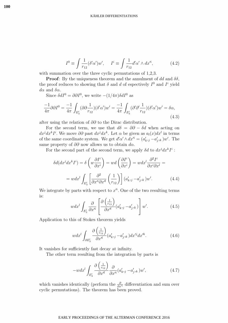
I0 ≡∫

1

r12(δ′α′)w′, I i ≡

∫1

r12d′α′ ∧ dx′i, (4.2)

with summation over the three cyclic permutations of 1,2,3.Proof : By the uniqueness theorem and the annulment of dd and δδ,

the proof reduces to showing that δ and d of espectively I0 and I i yielddα and δα.

Since δdI0 = ∂∂I0, we write −(1/4π)δdI0 as

−1

4π∂∂I0 =

−1

4π

∫E′

3

(∂∂1

r12)(δ′α′)w′ =

−1

4π

∫E′

3

(∂′∂′ 1r12

)(δ′α′)w′ = δα,

(4.3)after using the relation of ∂∂ to the Dirac distribution.

For the second term, we use that dδ = ∂∂ − δd when acting ondxjdxkI i. We move ∂∂ past dxjdxk. Let α be given as al(x)dx

l in termsof the same coordinate system. We get d′α′∧dx′i = (a′k,j −a′j,k )w

′. Thesame property of ∂∂ now allows us to obtain dα.

For the second part of the second term, we apply δd to dxjdxkI i :

δd(dxjdxkI i) = δ

(w∂I i

∂xi

)= wd

(∂I i

∂xi

)= wdxl ∂2I i

∂xi∂xl=

= wdxl

∫E′

3

[∂2

∂x′i∂x′l

(1

r12

)](a′k,j −a′j,k )w

′. (4.4)

We integrate by parts with respect to x′i. One of the two resulting termsis:

wdxl

∫E′

3

∂

∂x′i

∂(

1r12

)∂x′l (a′k,j −a′j,k )

w′. (4.5)

Application to this of Stokes theorem yields

wdxl

∫∂E′

3

∂(

1r12

)∂x′l (a′k,j −a′j,k )dx

′jdx′k. (4.6)

It vanishes for sufficiently fast decay at infinity.The other term resulting from the integration by parts is

−wdxl

∫E′

3

∂(

1r12

)∂x′l

∂

∂x′i (a′k,j −a′j,k )w

′, (4.7)

which vanishes identically (perform the ∂∂x′i differentiation and sum over

cyclic permutations). The theorem has been proved.

40


100


4.2 Helmholtz Theorem for Differential 2−forms inE3

The theorem obtained for differential 1−forms, here denoted as α, canbe adapted to differential 2−forms, β, by defining α for given β as

α ≡ wβ, β = −wα. (4.8)

Then, clearly,

wδ(wβ) = −dβ, wdβ = δ(wβ). (4.9)

Helmholtz theorem for differential 1−forms can then be written as

wβ = − 1

4πd

(∫E3

δ′(w′β′)r12

w′)− 1

4πδ

(dxjk

∫E3

d′(w′β′) ∧ dx′i

r12

),

(4.10)and, therefore,

β =1

4πwd

(∫E3

δ′(w′β′)r12

w′)+

1

4πwδ

(dxjk

∫E3


r12

).

(4.11)The integrals are scalar functions of coordinates x. We shall use thesymbol f to refer to them in any specific calculation. In this way, stepstaken are more easily identified.

The first term in the decomposition of β, we transform as follows:

wdf = (∂f)w = ∂(fw) = δ(fw), (4.12)

where we have used that w is a constant differential.For the second term, we have:

wδ(dxjkf) = w∂[wdxif)]− wd[fdxjk)]. (4.13)

The first term on the right is further transformed as

w∂(wdxif) = wwdxi∂f = −dxidf, (4.14)

where we have used that wdxi is a constant differential, which can betaken out of the ∂ differentiation. For the other term, we have

−wd(fdxjk)] = −wdf ∧ dxjk = −wf,i w = f,i = dxi · df. (4.15)

From the last three equations, we get

wδ(dxjkf) = −dxidf + dxi · df = −dxi ∧ df = d(dxif). (4.16)

41


101


In order to complete the computation, we have to show that d(wβ)∧dxi can be written as δβ ∧ dxjk. This can be shown easily by directcalculation. Let α be given as aidx

i. Then d(wβ) ∧ dx1 = dα ∧ dx1 =(a3,2 − a2,3)w. On the other hand, β = −aidx

jk and

δβ = (a3,2 − a2,3)dx1 + cyclic permutations. (4.17)

Hence δβ ∧ dx23 = (a3,2 − a2,3)w and, therefore,

d(wβ) ∧ dx1 = dα ∧ dx1 = δβ ∧ dx23, (4.18)

and similarly for the cyclic permutations of the indices.

5 Application 2: Cauchy like calculus with real dif-ferential forms

In chapter 2, we dealt with algebraic issues which were sufficient bythemselves to compute without resort to complex variable theory certaintypes of real integrals which are usually solved using that theory. Weshall now produce theory that involve operations which differential formsand that give results as if we were computing complex integrals.

When this author did all this work on this subject (two papers inarXiv), it was not too clear to him what was the most important fea-ture of what he was doing. He was distracted by whether an analyticfunction was defined by a power series (Weierstrass point of view) orby compliance with the Cauchy-Riemann conditions (Cauchy’s point ofview). But the difference is more profound; it lies somewhere else. Weproceed to explain this at length in subsection 5.3, after we had intro-duced the basis concepts.

The theory of complex variable not only deals with the solution ofthose real integrals, but is also used to solve integrals which are notreal. The question then is whether one can extend the theory of realdifferential forms so that it also comprises this new situation. One canextend it, and that is what this section is about.

5.1 Representation with real differential forms ofcomplex integrals

This section supersedes subsections 2.3 and 3.2 of our paper “Real Ver-sion of Calculus of Complex Variable: Cauchy’s Point of View”. Thatsubsection 2.3 is confusing and may be even misleading. It will now bemade unnecessary. As for subsection 3.2, it is clear but irrelevant since itdoes not clearly address the issue that will be considered here under theterm antivaluation. This is the operation opposite of valuation, rightly

42


102


considered there as in here. We think that its naturalness is here mademuch more clearly.

5.1.1 Valuations

The equivalence between i and dxdy is only algebraic. The unit i is aconstant and, as such, it can be taken out of an integral sign. But onecannot do so with dxdy, since it would change the nature of the inte-gral. So, one has to introduce a theory with real differential forms thatrepresents the calculus of complex variable through expressions where iis outside the integral. This takes place as follows.

With f(z) = u + iv and dz = dx + idy (which is correct, but whichwe might also write as ∂z = ∂x+ i∂y), we have∫

f(z)dz =

∫f(z)dx+ i

∫f(z)dy =

∫(u+ iv)dx+ i

∫(u+ iv)dy =

=

∫udx− vdy + i

∫udy + vdx = U + iV. (5.1)

for analytic functions, i.e. satisfying the Cauchy-Riemann conditions.Hence, we ignore the first equalities and focus on the last one. In thissection, we use the symbol w to refer to u + vdxdy. The last equationcan then be written as∫

udx− vdy + dxdy

∫udy + vdx = U + V dxdy, (5.2)

We replace integration∫cf(z)dz on a curve of the complex plane

with “valuation” 〈w〉c of an edif, u + vdxdy, on a curve c of the realplane:

〈w〉c ≡[∫

c

wdx

]+ dxdy

[∫c

wdy

], (5.3)

The integrability conditions for these integrals to not depend on c butonly on its end points are the Cauchy-Riemann relations. For u+vdxdy,this is the strict harmonic differential condition. “Valuation potentials”

〈w〉 = U + V dxdy =

∫udx− vdy + dxdy

∫(udy + vdx) (5.4)

then exist. Of course, U and V are undefined up to integration constants.The valuation on a closed curve (on simply connected manifolds) is zero.This is the Cauchy-Goursat theorem for strict harmonic differentials. Indomains that are not simply connected, we surround the poles enclosedby closed curves C with equally oriented circles ci, all of them with the

43


103


same orientation as C and containing one and only one pole each. Wethen have

〈w〉C =∑i

〈w〉ci . (5.5)

From now on, let us denote U + V dxdy as W. We have

∂W = dU + dV dxdy. (5.6)

SincedU = udx− vdy, dV = udy + vdx, (5.7)

we obtainU,x = u = V,y U,y = −v = V,x . (5.8)

W is, therefore, strict harmonic. Notice that we have not spoken off(x+ydxdy) inside of an integral sign. The Cauchy theory of differentialforms belongs to the elements of the algebra of even differential forms,not to the functions of some other variable.

5.1.2 Antivaluations

The valuation plays the role played by integration in the calculus ofcomplex variable. We shall refer to u + vdxdy as the antivaluation ofU + V dxdy. It is a simple matter to show that

dxdU = dydV dydU = −dxdV, (5.9)

anddUdx = dV dy dUdy = −dV dx. (5.10)

The antivaluation can be given in a variety of ways:

u = dx · dU = dy · dV = idy ∧ dU = −idx ∧ dV (5.11)

andv = dx · dV = −dy · dU = idx ∧ dU = idy ∧ dV. (5.12)

i referring, of course, to dxdy.To strengthen ideas, let us see what f(z) = z = x + iy, df/dz = 1

corresponds to. We compute the antivaluation for U = x, V = y. Weget u = dx ·dU = dx ·dx = 1 and v = dx ·dV = dx ·dy = 0. So, x+ydxdyis a primitive of 1. We check it computing the valuation:∫

1dx+ dxdy

∫1dy = x+ ydxdy. (5.13)

44


104


5.1.3 Cauchy calculus versus exterior and Kahler calculi

The contents of the previous two subsubsections can be taken as thefoundations of a Cauchy calculus of strict harmonic differential forms.The Cauchy calculus is different from the Kahler calculus of differentialforms, since it is based on a different concept of integration and differ-entiation. What goes by the concept of integration and differentiationin the calculus of complex variable has a correspondence in valuationsand antivaluations in the Cauchy calculus of differential forms. The factthat this calculus uses the Kahler algebra might lead one into confu-sion. Readers might be right in thinking that this section belongs to theprevious chapter. This is logically correct, but consider this. A Kahlercalculus on a Kahler algebra is far more important than a Cauchy calcu-lus on the same algebra. It is better to be confused learning this Cauchycalculus after having learned the Kahler calculus than to be confusedlearning the latter after having learned the former.

Let me insist on the point just made. In the Kahler calculus, dif-ferential r−forms are evaluated (i.e. integrated) on r−surfaces. In theCauchy calculus of differential forms presented so far, we “valuate” evendifferential forms on curves. The valuation on curves involves the inte-grating or evaluation on those curves of associated differential 1−forms,specifically the differential 1−forms udx− vdy and udy + vdx.

dU = udx− vdy, dV = udy + vdx. (5.14)

Properly speaking, an expression such as dz = dx + idy does notpertain to the complex variable calculus proper, but to the representa-tion in the plane of differential forms over the complex numbers. Theobtaining of dz through differentiation belongs to the exterior calculusof these differential forms, not to the calculus of complex variable, wheredifferentiations take place with respect to z.

Let us use define Z = x+idxdy. It is certainly the case that dz = dx+idy and that, in contrast, dZ = dx. But, as we have explained, d(z) =dx+ idy is not a differentiation in the calculus of complex variable andd(Z) = dx is not a differentiation in the Cauchy calculus of differentialforms. We cannot make anything of this difference.

The differentiation of z in the calculus of complex variable is simplydz. End of story. We can of course write dz = (dz/dz)dz = dz. In thecalculus of complex variable, the differentiation of x takes place throughthe differentiation of x = (z+z∗)/2. This poses problems when trying todifferentiate z∗, for which purpose one resorts to a representation in theplane. See, for instance, H. Cartan’s “Elementary Theory of AnalyticFunctions of One or Several Complex Variables”. He introduces z and z∗

for the first time in his book as follows: “Recall that a complex number

45


105


z = x + iy ... is represented by a point on the plane ... If we associatewith each complex number z = x + iy its ‘conjugate’ z = x − iy...”.Of course, H. Cartan knows better. Later in his book he considersdifferentiations with respect to the complex variables z and its conjugatez and introduces the Laplacian as ∂2f/∂z∂z. And later, when dealingwith n complex variables, he writes

df =n∑

k=1

(∂f

∂zkdzk +

∂f

∂zkdzk

), (5.15)

for the differential of a function of so called n complex variables. Whenthis is done, d(x+iy) = dz through a process where x and y are expressedin complex variable terms.

This discussion was worth writing for an indirect purpose: as refor-mulated, the exterior calculus of one complex variable can be seen as atheory of strict harmonic differentials. Forget about functions of x+ iy.That may be included in the game, specially as a bridge to start thegame, like even the most notable mathematicians do. But, once again,we did not use x+ydxdy above. And, if one uses it and the likes of it, weshall have to take into account that the relation between “the complexvariables” x+ ydxdy and x+ zdxdz will not be the same as the relationbetween x + ydxdy and z + tdzdt, assuming of course positive definitemetric. Indeed dxdydxdz equals a differential 2−form; dxdydzdt is adifferential 4−form. Its interior derivative is not a differential 1−form.

We have set the stage for a Cauchy theory involving strict harmonicdifferential forms in Euclidean spaces of arbitrary dimension, not spacesof several complex variables. It is a theory much richer than standardtheory of several complex variables.

5.2 Cauchy’s theorems

This subsection should be about Cauchy’s integral formula and Cauchy’sintegral formula for derivatives. They are clearly explained in subsec-tions 3.1 and 3.3 of our paper “Real Version of Calculus of ComplexVariable: Cauchy’s Point of View”. Although we have said that theCauchy theory of differential forms belongs to the elements of the alge-bra of even differential forms, not to the functions of some other variable,using the notation f(z) instead of f(x + ydxdy), which in turn we usethere instead of u + vdxdy, has notational advantages. The nature ofthose theorems is at the root of those notational advantages.

See the same reference for a couple of exercises.

46


106


CHAPTER 4: RelativisticQuantum Mechanics

Jose G. Vargas

Once again, lecturers will choose from this chapter what they willteach on day 6 of the summer school.

This chapter was going to be called Kahler equations. I changed thetitle when I recently learned that a group of billionaires (like Ambani,Bezos, Branson, Gates, Ma, Soros, Zuckerberg, etc. is launching a majorclean energy initiative (For fair treatment of those that I have not men-tioned, please go breakthroughtenergycoalition.com/en) Energy is anissue for exceptionally good theoreticians, like Einstein in the first half ofthe twentieth century (energy of photons, energy equalsmc2, the energy-momentum tensor equals the Einstein tensor) and Julian Schwinger (Seethe last section of this chapter for more on Schwinger, the other Feyn-man or even better) in the second half. The ideas of both, Einstein andSchwinger, in the last decades of their lives were dismissed. In the lastsection, we also say a little bit about the connection between Kahler’scalculus and Einstein’s failed at unification with teleparallelism.

Kahler’s quantum mechanics (actually, the Kahler equation by itself)has to do with the initiative of the coalition, even though its proponentsdo not know it. It prompts and promises a better understanding of en-ergy at the quantum level. Present day quantum physics is being builtwith inadequate arguments, which are at the root of the spurious emer-gence of negative energy solutions in Dirac’s theory. It is resolved bymeans of so called “hole theory”, where all states with negative energyare filled and thus constitutes a sea of infinite energy density. Holes (orlack of negative energy solutions) are interpreted as positrons (A verygood book for all of this is “Relativistic Quantum Mechanics” by J. D.Bjorken and S. D. Drell, both from the Stanford Linear Accelerator Cen-ter”; its chapter five is about hole theory). The infinite energy densityof the sea is reduced to still huge finite ones through a couple of inde-pendent artifacts which do not even give the same results (They actually

47

107


give results that differ by dozens of orders of magnitude). In contrast,Kahler’s equation entails the emergence of positrons with the same signof energy as electrons. Since we reserve that derivation for chapter six,we send impatient readers to the very end of section 26 of Kahler’s 1962paper “Der innere Differentialkalkul”.

Also recently —while writing these chapters— I heard again the of-ten repeated statement that quantum physics and general relativity aremathematically and conceptually incompatible. But, with the Kahlercalculus, the mathematics of general relativity are contained in the math-ematics of quantum mechanics. They are not, therefore, mathematicallyincompatible. As for conceptual incompatibility, it is not so because ofthe nature of the subject but because of the Dirac equation. In his time,it was a tremendous conquest, but provisional and not quite as intelli-gible as physics used to be). Its limitations led to misinterpretations asto the true nature of the field. If, as this author claims, the Kahler cal-culus is the right equation, the quantum mechanics that ensues is moreabout a field in the classical mold rather than about particles and prob-ability amplitudes. The latter (certainly as well as their square) shouldbe viewed as derived or emergent concepts. But does one really believethat the mathematics for both sectors of physics they will incompatiblefor ever? We should not replace ”we do not know how to do ...” with”it cannot be done”. And, fortunately, Kahler’s version of quantum me-chanics is such that the day to day practice of most of quantum physicswill not change; only the foundations will.

In order to provide an early glimpse of Kahler’s approach to quantumphysics, we shall alter for the summer school what should have been theorder of chapters in the presentation of the theory. In this chapter, weshall mention, though only briefly, Kahler’s obtaining of the strict har-monic differentials in 3-D Euclidean space (minus the origin), where theycoincide with the harmonic differentials. Such a study should logicallyfollow the study of rotational symmetry (chapter 5), which is instrumen-tal in solving the fine structure of the hydrogen atom. We shall leave forreaders to follow the long calculations directly from the Kahler papers,which they should be able to read with little knowledge of German afterwe have provided here the basic foundations. Chapter 6 will deal withthe conservation law and related applications (the two types of charge,a uniqueness theorem for integration of Helmholtz type systems, etc.).

Starting with chapter 7, I would present my own work on the Cartan-Kahler calculus of differential forms, where physics and mathematicslook as if they were the same thing. Fortunately for participants in thissummer school, you will not have to suffer me much longer since, bythen, it will be the early morning of the last day of the school.

48

RELATIVISTIC QUANTUM MECHANICS

108


What does all this have to do with the breakthrough energy coali-tion? A better platform for quantum mechanics is a better platform forunderstanding energy. One could bring the Kahler calculus —and thusquantum physics and the understanding of energy— to greater heightswith an amount of funds that would be pocket money for billionaires,specially if the funds are used in countries where eager scholars drawmeager salaries. I have written this for the record so that one day, per-haps not too far for me to see it, mathematically gifted acquaintancesof those billionaires let them know of this opportunity to carry on theirproject with the much more sophisticated Kahler theory. It may lead toless costly and more efficient and environmentally friendly way of obtain-ing clean energy. Schwinger may have pointed the way with his sourcetheory, and Kahler mathematics is the right tool to make his theorymore accessible.

1 Kahler equations

With the explicit purpose of accelerating the bringing about of a morecomplete picture of what the Kahler calculus has to offer, I am startingto skip details of computations present in Kahler’s papers.

1.1 Solutions with time symmetry of exterior sys-tems

The form of solutions with symmetry of exterior systems is independentof the system itself. We mean what types of factors represent the sym-metry in solutions that have it. The dependence on coordinates thatare parameters of symmetries is given by a phase factor, and the de-pendence on their differentials is given by idempotents that are constantdifferential forms.

Recall a decomposition such as

u = +u ε+ + −u ε−. (1.1)

It corresponds to time translation symmetry. The phase factor must,therefore, be e−iEt. As we shall son start to understand and with = 1,a negative charge solution with time translation symmetry should begiven by

e−iEtR(x, dx)ε−. (1.2)

By virtue of the fact that the ε± are constant differentials, we shall haveequations

∂u = (∂ +u) ε+ + (∂ −u) ε−, (1.3)

49


109


implicit in the more comprehensive equation

∂u = (∂ +u+) ε+τ+ + (∂ +u−) ε+τ− + (∂−u+) ε−τ+ + (∂−u+) ε−τ−

(1.4)for when, in addition to time translation symmetry, one also has rota-tional symmetry (See chapter 2 for all these idempotents). Suffice torewrite this equation as

∂u = [(∂ +u+) τ++(∂ +u−)τ−] ε++ [(∂−u+) τ++ (∂−u+)τ−]ε− (1.5)

and then as

∂u = ∂(+u+ τ+ + +u−τ−) ε+ + ∂(−u+ τ+ + −u+τ−)ε− (1.6)

τ± has to do with issues that come under the name of handedness,chirality and helicity, intrinsically associated with spin. This will beunderstood when, in the next chapter, we deal with angular momentum.

For a system where the rest mass of the electron were the dominantenergy, it makes practical sense to write E asm+∆E. This is well knownfrom standard relativistic quantum mechanics. In the Kahler calculus,the dominant energy representation of electron systems is given us

u = e−imtR(t, x, dx)ε−, (1.7)

where R(t, x, dx) depends the more slowly on time the more close to eachother m and E are. Compare with (1.2). This expression for solutionswill be very much used in the following.

1.2 Kahler equations for stationary solutions

Let u be any element of the Kahler algebra (again, of scalar-valueddifferential forms). Any equation of the form

∂u = au (1.8)

will be referred to as a Kahler equation. A particular case is ∂u =0. In Euclidean space of dimension 2 we get even differential forms,already considered in the two previous chapters. In dimension 3, Kahlerderived a magnificent theory of harmonic differentials without resort toseparation of variables. That is very interesting but momentarily, it isnot as important as the equation (1.8) in spacetime, with a differentfrom zero and the algebra being over the complex field. We shall alsomake c = 1.

(∂±u)ε± = a (±u ε±). (1.9)

50


110


Solutions ±u ε± may correspond to particle states of undefined chirality.From the perspective of the number of components in the solutions

and what they represent, neither Eq. (1.8) nor Eqs. (1.9) have a closeanalog in the Dirac equation. To start with, they do not have the samenumber of components. The electron and positrons of both chiralitiesare directly associated with the equations

(∂ ±u∗)ε±τ ∗ = a (±u∗ ε±τ ∗). (1.10)

The parentheses have been put there simply to emphasize that the dif-ferentiation of ε±τ ∗ can be ignored since it yields zero. The asteriskmeans that correlation between the superscripts of ε and τ is not im-plied. The ε± would be for pairs of particle and antiparticle, and theτ± would be for the two opposite handedness in each of those two cases.Phase factors are inside the ±u∗ when solutions proportional to ±u∗ ε±τ ∗

represent specific particle states.By writing a as α+ iβdt and replacing ±u with e−iEtp±, the develop-

ment of Eqs. (1.9) by Kahler yields the following equations for stationarysolutions

∂p± (E + β)ηp − αp = 0, (1.11)

where the signs ± corresponds to p± respectively. This is obtained with-out resort to dominant energies or specific couplings. Kahler used thisequation just for the fine structure of the hydrogen atom, for which ittakes a very simple form. We shall later see another important applica-tion.

1.3 Kahler equations for Dirac spinors

We may be interested in what we shall denote as Dirac spinors that areproper “functions” for given energy and chirality. Kahler wrote suchspinor solutions as

u = eisφ−iEtpτ±ε∗, (1.12)

where p depends only on ρ, z, dρ and dz, and where s and E are theangular momentum and energy of the system. We shall replace thesymbol ∨ for juxtaposition when we judge that it makes equations moretransparent.

Differentiating (1.12), we get

∂u = eisφ−iEt(isdφ ∨ p− iEdt ∨ p+ ∂p)τ±ε∗. (1.13)

We then usedφ ∨ p = dφ ∧ p = ηp ∧ dφ = ηp ∨ dφ, (1.14)

anddt ∨ p = dt ∧ p = ηp ∧ dt = ηp ∨ dt. (1.15)

51


111


Thus,

∂u = eisφ−iEt(is ∨ ηp ∨ dφ− iEηp ∨ dt+ ∂p)τ±ε∗. (1.16)

We now use that

τ− − τ+ = −idxdy = −iρdρdφ (1.17)

to obtain dφ and then

dφ ∨ τ± = −idρ

ρ(τ− − τ+)τ± = −i

dρ

ρτ±. (1.18)

Equation (1.18) together with idtε± = ∓ε± allows us to finally write(1.16) as

∂u = eisφ−iEt(∂p± sηpdρ

ρ− ∗Eηp)τ±ε∗, (1.19)

which could be used on the left hand side of Kahler equations, specially ifwe do not want to resort to dominant energies in reducing the simplicityof some Kahler equations.

2 Dominant energy and electromagnetic coupling

In the first subsection of this section as well as everything that wentabove is original work of Kahler. If you do not like it, go to church andtalk to him. From now on, I take the blame for what follows. I say thatbecause some learned people will retort that this is not in the spirit ofmodern physics and mathematics, or they will say even something worse.I do not care. The mathematical and physics community should at leastknow what Kahler did. He wrote in German. I am doing it in Englishand in a slightly more Cartanian way. One has to understand geometrya la Cartan in order to really appreciate the Kahler’s calculus and evengo beyond it. With my book ”Differential geometry for physicists andmathematicians” I tried to do with some of Cartan’s work what I amnow trying to do with some of Kahler’s work.

2.1 Charge

With electromagnetic coupling, the Kahler equation reads

∂u = (−m+ ieA)u, (2.1)

where m is the rest mass, and e (positive or negative) represents thecharge of positrons and electrons. In going from (1.8) to (2.1), there areunstated or undefined assumptions. We are trying to say that, whereas(1.8) does not assume a situation where particles and antiparticles are of

52


112


the essence, (2.1) does, even though this is not explicit. It is containedin the mere presence of a mass competing with an electromagnetic field.For the split (1.1),we have

(∂±u) ε± = (−m+ ieA) ±u ε±. (2.2)

Let us now deal with the announced existence of what, in the elec-tromagnetic case, becomes charge of opposite signs. We shall reproducein chapter 6 the derivation of the conservation equation of this calculusand its specialization to when u is written as (1.1). After the appro-priate natural interpretations, the conservation law takes a form whichtranslated to the language of the vector calculus reads like this

(∂ρ+∂t

+ div j+

)+

(∂ρ−∂t

+ div j−

)= 0, (2.3)

where ρ+ and j+ are determined only by +u and its complex conjugate,and similarly for ρ−, j+ and j−. Hence the two options in ε± should beassigned to positrons and electrons. Probability densities should in turnbe assigned directly to charge and indirectly to particles, but certainlynot yet at this point.

We shall not go until chapter 6 into the rather laborious derivationof how ρ± and j± depend on ±u. Equation (2.3) implies the apparentexistence of two types of charge, and that only total charge (understoodas their sum) and not each individual one is conserved when both arepresent. Their individual conservation is an afterthought when the twotypes stay apart, like a nucleus and its surrounding cloud of electrons.

In obtaining (2.3), Kahler does not make full use of the Kahler equa-tion with electromagnetic coupling, but simply that a for that couplinghas a specific property, which can also be satisfied in principle by otherones. And even if that property were not satisfied, we might still getconservation equations with the flavor of (2.3), but where the ρ’s andj’s would depend on the ±u’s in a different way. Results like this do notmake part of the books on the Dirac theory from which I, and probablyyou, learned.

The equations we derived in the previous section can easily be adaptedto the electromagnetic coupling. We are about to see that the equationsfor positrons and electrons have nothing to do with small and largecomponents of the solutions of one equation, solutions misinterpreted inthe Foldy-Wouthuysen treatment of Dirac’s theory as respectively repre-senting positron and electron amplitudes. Large and small componentsbelong equally to solutions for particles and antiparticles. These two arein the same footing at this level of theory.

53


113


2.2 The Pauli equation

Of practical interest is the case when the rest energy m of the electronis the dominant energy. We use (1.7) in (2.1) for an electron in a stateof undefined handedness in an electromagnetic field. Given that ∂u isdt u,t + dxi u,i, we get, after some simplification,

[dt(−imR +R,t ) + dxiR,i

]ε− = (−m− ieΦdt+ ieAidx

i)Rε−. (2.4)

Premultiplying by −dt, using that (dt)2 is −1 and leaving R,t ε− as the

sole term on the left, we get

R,t ε− =

[−dxidtR,i +(−ieAidxidt+ im+mdt− ieΦ)R

]dtε− (2.5)

We cannot simplify ε− until we absorb all dt factors into ε−, which wedo by means of dtε− = −iε− (Check what would happen and comparewith what we are about to get). We thus obtain

R,t = −PηR− ieΦ + im(R− ηR), (2.6)

where we have replaced dxj(−i∂j−eAj) with the symbol P and where wehave used that R does not contain dt as a factor. Recall from previouschapters that η changes the sign of terms of odd grade. We apply η to(2.6). Combining the resulting equation with (2.6) itself, we get

ϕ,t = Pχ− ieΦϕ, (2.7)

χ,t = −Pϕ− ieΦχ+ 2imχ, (2.8)

where

ϕ =1

2(R + ηR), χ =

1

2(R− ηR). (2.9)

We now proceed following a step to be found in the standard literature.Among the books on relativistic or advanced quantum mechanics thatwe have come across, there is one which deserves special attention be-cause of the topics it deals with, namely the aforementioned “RelativisticQuantum Mechanics” by J. D. Bjorken and S. D. Drell”. This book isparticularly interesting not only because of the institutional affiliation ofits authors and the contributions they made to the high energy physicsof their time, but also because of the year in which their work was pub-lished, 1963. That was the time when high energy physics was becomingcorporate physics, meaning that advances were produced as if they wereproducts of a corporation, one of the main headquarters being Stanford’slinear accelerator. It was also the time when problems in the very foun-dations of quantum mechanics were addressed rather than swept under

54


114


the rug, as, more often than not happens nowadays. This is why therewas a chapter on hole theory in their book. We have mentioned all thisbecause we are about to take a step right now which is conceptually thevery same step as one of those that they took in their first chapter. Inthe paragraph just before the last, they had connected with the Pauliequation. They then opened the last paragraph of the chapter as fol-lows: “Fortified by this successful non-relativistic reduction of the Diracequation, we go on ...”

The title of their chapter 4 is “The Foldy-Wouthuysen transforma-tion”. And chapter five’s title is “Hole theory”, designed to deal with theissue of negative energy solutions of Dirac’s theory. These solutions area consequence of what is spurious in Dirac’s theory. The association ofantiparticles with negative energy solutions does not emerge when doingrelativistic quantum mechanics with Kahler’s mathematics.

In the process of deriving the Pauli equation, Bjorken and S. D.Drell took a step which is totally equivalent to the one that we areabout to take with our equation (2.8). Of their equation that parallelsthis equation (2.8), they said that “it may be approximated for kineticenergies and field interaction energies small in comparison with mc2, ...”.We return to this further below, where we shall see that this amounts toneglecting terms χ,t and −ieΦχ in our equation (2.8). The assumptionχ,t is unwarranted, since χ,t may be huge and can thus not be ignoredeven if χ,t were small. This will have a very important consequence thatis worth mentioning with a view to trying to understand at least someobscure point in the Dirac theory, as we shall explain further below. Letus assume that we ignore this difficulty and proceed in parallel to whatthey did. If the said approximation were correct, we would have

χ1 = − i

2mPϕ, iϕ′,t = iPPϕ+ iΦϕ. (2.10)

Let us assume that we knew ϕ. We would then approximately know χ.We refer to this approximated χ as χ1. With χ replaced with χ1, theright equation (2.7) gives only an approximate ϕ,t even if we knew theright ϕ and left it on the right. This is the reason why we have usedϕ′ on the left and ϕ on the right. This remark will be useful for theapproximation in the next section

We expand PPϕ and use that

PkPjϕ = −i∂k(ieAj) = ieAj,k . (2.11)

We then perform some manipulations given in more detail in our “TheFoundations of Quantum Mechanics and the Evolution of the Cartan-

55


115


Kaehler Calculus” (Foundations of Physics 38, 610-647 (2008)), and get

i∂

∂tϕ′ =

1

2mP 2ϕ+

ie

2mBkdx

idxjϕ+ eΦϕ, (2.12)

where the summation is over the three cyclic permutations of (1, 2, 3).This is the Pauli equation in terms of differential forms, except thatPauli’s ϕ on the right hand side also is ϕ′. At this stage and for thepresent purpose, “this difference does not make a difference”.

One should not overlook that this equation is for ϕ, not for R, here asin the corresponding formula in the Dirac theory. In spite of the objec-tion raised about (2.10), equation (2.12) is of great interest,. though notfor the same reason as in the paradigm, where it was welcome because itgave confidence in the Dirac equation to construct a relativistic theoryof the electron. For us, it will be important for another reason, whichwe shall discuss at length later on.

2.3 The Foldy-Wouthuysen Hamiltonian

In the literature, one uses the term Foldy-Wouthuysen transformationmore often than Foldy-Wouthuysen transformation. But its main pur-pose is the transformation of the Hamiltonian, which Bjorken and Drellperform in the every same section. In fact, they do not even speak of thetransformed wave function on which the new Hamiltonian acts, thoughthis is obvious by gauge invariance considerations.

We continue the process by which (2.12) was obtained. We write thesought χ as the old one, χ1, plus some χ′

1,

χ = − i

2mPϕ+ χ′

1. (2.13)

This together with (2.8) yields

χ,t = −ieΦχ+ 2imχ′1. (2.14)

Hence, solving for χ′, we have

χ′1 =

i

2mχ,t +

eΦ

2mχ. (2.15)

From (2.7), we get that χ′1 adds the terms iPχ′

1, i.e.

iPχ′1 =

−1

2mPχ,t +i

eΦ

2mPχ. (2.16)

It is only at this point that we replace χ with χ1 on the right hand sideof (2.16). The computations are straightforward but rather laborious.One obtains

iPχ′1 =

−1

8m3p4ϕ− i

e

4m2PECϕ− e

4m2Ei , jdx

j ∧ dxiϕ, (2.17)

56


116


where we have eliminated higher order terms for comparison purposeswith how this would be written in the paradigm. The small p is −idxj∂j,and E is here notation for dxjEj. The superscript is used to indicatethat E in PECϕ is treated as if it were a constant in this term. Theparenthesis around dxj ∧ dxi is meant to say that we add over cyclicpermutations in 1kdxi ∧ dxj.We thus further get

− ie

4m2PECϕ = − e

4m2dxidxjEj∂iϕ, (2.18)

which corresponds to the σ · (E× p) term in the standard version of rel-ativistic quantum mechanics, i.e. with vector-valued quantities. Pleasebe informed that we had an inadvertent replacement of a “∨” productwith a “∧” product. That in turn gave rise to a spurious term, which isthe reason for a discrepancy with (2.18).

The last term in (2.17) yields

− e

4m2Ei , jdx

j ∨ dxiϕ =e

4m2Ei,i ϕ− e

8m2Ej ,idx

j ∧ dxiϕ, (2.19)

equivalently, the divE and σ · curlE terms with appropriate factors. Inall terms on the right of the i ∂

∂tϕ′ post-Pauli equation, all operators are

acting on ϕ the original wave differential form ϕ.Let us look at what we have got. We have developed to order 1/m3

the Kahler equation with electromagnetic coupling and mass as domi-nant energy term for the even grade part of solutions whose odd gradepart satisfies χ,t −P ∨ ϕ. The development was directed towards let-ting i ∂

∂tϕ alone on the left hand side. Hence, the right hand side defines

a Hamiltonian, namely

H =1

2mP 2 +

ie

2mBkdx

idxj + eΦ− 1

8m3p4 − e

4m2dxidxjEj∂i

+e

4m2Ei,i − e

8m2Ej ,idx

jdxi, (2.20)

acting on the original wave function, whereas the energy operator, i∂/∂tis acting on a slightly different wave function, i.e.

i∂

∂tϕ′ = Hϕ. (2.21)

Of course, we could think of ϕ′ as a ϕ, and vice versa, thus i ∂∂tλ = Hλ′,

where we have used λ′s instead of ϕ’s in case it would create confusion.Observe how, by virtue of the little bit of Kahler equations that we

have learned, we have reached deep into relativistic quantum mechanics,to a depth even greater than most advanced books on quantum mechan-ics.

57


117


2.4 Leftovers

TO BE COMPLETED. This subsection would deal with subjects thatwe left over because of the pressure for this author to write about otherjewels of this calculus and concomitant quantum mechanics.

Readers can now do exactly the same for positrons. One only has torepeat with

u = e−imtR(t, x, dx)ε+, (2.22)

what we did with e−imtR(t, x, dx)ε−. You will find a system just like(2.7)-(2.8), except that the even, ϕ, and odd, χ, parts of u will satisfythe equations satisfied by χ and ϕ. Thus ϕ will be small and χ will belarge under similar assumptions. But notice that both χ and ϕ belongto the electron and both ϕ and χ belong to the positron. Whether wehave one particle or another depends only on whether we are dealingwith ε+ or ε−.

Another topic that will be treated in this subsection is the explana-tion from the Kahler theory of why the mass of the positron emerges as−m. In this and following chapters, I shall provide you with entries intothe world of Kahler, exploring areas that nobody has jet explored.

3 An entry point for research on relativistic quan-tum mechanics with the Kahler calculus

What follows might be felt as being derogatory on Dirac, whom manywill rightly consider the second best physicist of the twentieth century.His equation presently is more relevant for theoretical physics than Ein-stein equations. Dirac did his work when the math was not ready forthe task. So, thanks are due to Dirac. But now is now and the math-ematics allows for a better job. We proceed to describe the situationwith respect to post-Pauli-Dirac electromagnetic Hamiltonians. For thediscussion that will follow, we write the Dirac equation with explicituniversal constants

i∂ψ

∂t=

[cα·

(p− e

cA)+ βmc2 + eΦ

]ψ, (3.1)

where α and β represent well known matrices in relativistic quantummechanics. Clearly, a development in powers of 1/m, which is whatBjorken and Drell did, is not equivalent to a development in powers of1/c. The reason to make this remark will be seen later below.

58


118


3.1 Post-Pauli-Dirac and Foldy-Wouthuysen equa-tions

The term Foldy-Wouthuysen Hamiltonian is not used in the literature.One uses instead the term Foldy-Wouthuysen to refer to transformationsthrough which one reaches the Hamiltonian:

H = β

(m+

(p− eA)2

2m− p4

8m3

)+ eΦ − e

1

2mβσ ·B

− ie

8m2σ· curl E − e

4m2σ(E× p) − e

8m2divE, (3.2)

where p has components pi, where Φ and A are components of the4-vector potential and where σ has as components the three Pauli ma-trices. Equation (3.2) results in the approximation (kinetic energy/m)3

and (kinetic energy)(field energy)/m2. The Hamiltonian (3.2) is the tan-gent vector field equivalent of (2.20), except for the absence of the massterm in the latter and for a factor of two in the divergence of E term.The three terms in the parenthesis in (3.2) and the five terms outside itadd to eight. Terms 1, 2, 3, 4, 5,6 and 7 of (2.20) correspond to terms2, 5, 4, 3, 7, 8 and 6 of (3.2). The reason for the absence of the m termhas already being explained. What is surprising tis that all the otherterms are the same except for the factor of two to which we have justmade reference

We follow the presentation by Bjorken and Drell. This is a Hamilto-nian that displays the different interaction terms between the electronand an applied field in an easily interpretable form. They do not give theform of the equation or on what “function” (actually a two componentspinor) this operator is acting upon. We shall see further below why thisremark is important.

They apply a unitary transformation three times. The purpose indoing so is to remove all from the equation all operators such as αwhich couple the large to the small components. It is implicit in thisthat the equation where (3.2) would be the Hamiltonian is an equationfor the positive energy state. More on this below. They describe aFoldy-Wouthuysen transformation as “a canonical transformation whichdecouples the Dirac equation into two two-component equations; onereduces to the Pauli description in the nonrelativistic limit; the otherdescribes the negative energy states.”

In speaking of negative energies, they state that they “and four-component wave functions are the price we must pay in order to havea factorization of H ′ in (4.1) into a linear Dirac equation.” H ′ is theoperator

H ′ = β√

m2 + p2. (3.3)

59


119


It is worth noticing that the Kahler equation was born linear, and thatnegative energy solutions need not accompany the positive ones. Thereis not an ab initio need to separate them if we start with a spinor in theright ideal, and small components, when dealing with the electron, donot then belong to the positron.

We now cite on the Foldy-Wouthuysen transformation from the book“Relativistic Quantum Mechanics and Introduction to Field Theory” byF. J. Yndurain. Let us start with “... of the four solutions of the Diracequation (with or without a potential) only two are physical”. Makewhat you want of such a statement. You would find in every book onthe subject some statement who makes you raise your eyebrows, thoughany such statement does not raise the same eyebrows.

Yndurain performs two Foldy-Wouthuysen transformations on “theDirac for a particle in a potential, the sum of a Minkowski vector (A,A0), a Minkowski fourth component, V0, and a scalar one, βVS :

H = mc2β + V + VSβ + cα·(P− e

cA); (3.4)

we have here defined V ≡ A0 + V0”. Here P is the usual p. His resultfor “the Foldy-Wouthuysen Hamiltonian” is

HFW = mc2β + V + VSβ + β(P− eA)2

2m− e

1

2mβσ ·B− β

P4

8m3c2

− 1

8mc2[αP, [αP,V ]]− 1

8mc2β αP,αP,Vs . (3.5)

The author has performed two Foldy-Wouthuysen transformations. Act-ing on operators (call them h) to the left of the spinor, each Foldy-Wouthuysen transformation yields take eThe−T . Under the two trans-formations, the positive energy solutions of the Dirac equation are rep-resented by wave functions

ψFW = eT′eTψ +O(c−3). (3.6)

(O(c−3) as in the original). We were interested in this comment, whichcertainly we are not criticizing. He is certainly treating Foldy-Wouthuysentransformations as gauge transformations. Hψ will go into

(eT′eTHe−T e−T ′

)(eT′eTψ) = eT

′eTHψ. (3.7)

Hence, the Dirac equation written as i∂ψ/∂t = Hψ goes to

HFWψFW = ieT′eT

∂ψ

∂t= i

∂ψFW

∂t. (3.8)

60


120


Let us finally consider one more approach to the Hamiltonian in apost-Pauli approximation. In the first part of their volume (IV) on Rela-tivistic Quantum mechanics, Landau and Lifchitz reportedly reproducethe treatment of A. Akhieser an V. Berestetski to reach the next ap-proximation in the development of (3.1), They say that they assumethat there is only an electric field. They set A = 0 and obtain

H =p2

2m+ eΦ− p4

8m3− e

4m2σ · (E× p)− e

8m2divE. (3.9)

Again, the method followed causes the absence of the m term. Theabsence of them term, as was the case with (2.20) has to do with the factthat they intended to obtain the next approximation for a Schrodingertype equation.

Also absent in (3.9) are the terms 5 and 6 of (3.2). The absence ofterm 5 is not surprising given that they have assumed A = 0. But theabsence of term 6 might be attributed to the fact that making A = 0makes the electric field incomplete. There is no discrepancy between thedivE term in (3.2) and (3.9). We do not know where the discrepancy bya factor of two with a similar term in (2.20) is born.

3.2 Research suggestions for involvement with theKahler calculus

Without the need for further comparisons, it is fair to say that thesedevelopments of the Dirac equation are not very transparent. Our de-velopment of the Kahler equation is, but it remains without explanationwhy we should be satisfied with an equation for ϕ rather than an equa-tion for u. It would be desirable to approach the problem without theearly separation of the equation for u into ϕ and χ I suggest readershave here an entry point for research on relativistic quantum mechan-ics with the Kahler calculus. I suggest the following two problems. Ihave not even started to do what I am suggesting for fear of gettingtoo involved with them at a “time when I do not have time”. So, I donot know whether one gets something of interest and/or easy to handle.Much will depend on the ability of those who may try.

Research problem. Since the β of equation (1.11) is a 0−form,we can solve for ηp. This can be replaced in the equation obtained byapplying η to (1.11). At this point, it will be useful to see what thisequation says after replacing α the β for electromagnetic coupling readfrom (2.10). It seems clear that this will not be directly comparable to(2.20), (3.2) and (3.3) since it will involve the potential rather than theelectric and magnetic fields. One can then proceed with different typesof approximations only limited by your imagination.

61


121


Research problem. One can then try to follow the same processnow with (1.19), where the chirality or handedness of the state differen-tial form is defined.

4 Breakthrough energy, Kahler calculus and Schwinger’ssource theory

Dirac’s theory carries a baggage that Kahler’s does not. The formerhas been loaded since birth with the concept of spinor as fundamental,rather than emergent (Notice that u does not even represent a particle inEq. (1.8), and a need not contain the mass). We want to extract cleanenergy from wherever. matter holds the greatest density of energy. But,at the nuclear level, energy is not sufficiently well understood. What wehave seen in previous sections should be enough to make the point thatKahler’s theory holds promise in this regard because it is more powerful,more structured and more comprehensive. Its connection with nuclearphysics may be in source theory.

4.1 Schwinger’s source theory

The modern expansion of Dirac’s theory, with concepts like spin connec-tion, comes at a stiff price and does not even have the right generality. Inthe first of the already posted chapters, one sees that the Kahler deriva-tive of vector-valued differential forms also depends on the connectionon the manifold. Unlike the spinor connection, it will not generally in-volve Christoffel symbols, either directly or exclusively, unless the affineconnection of the manifold is the Levi-Civita connection. To make mat-ters worse, dealing with the generalization of the Dirac operator requiresyears of specialization by those who eventually work with it. And whathas been achieved with it?

As in Dirac’s, the concept of mass is not yet emergent in Kahler’stheory, but the concept of mechanical and generalized momentum is.Concepts like Foldy-Wouthuysen transformations are unnecessary andcloud the issues. Also in the Kahler calculus, the treatment of the en-ergy operator (we leave the imaginary unit factor for the last day ofthe summer school) and of Hamiltonians is just a matter of comput-ing with differential equations without resort to operator theory. Andmost significant is the fact that Kahler’s treatment of angular momen-tum is just a matter of Killing symmetry and properly handling sums ofpartial derivatives, rather than replacing operators for classical particlemagnitudes. Our treatment of relativistic quantum mechanics withoutoperator theory should have made plausible the idea that cutting edgequantum physics need not be quantum field theory, which is operator

62


122


based. Nor is the by now forgotten S-matrix theory a suitable alter-native. We anticipate that a third option, Schwinger’s source theory,constitutes a proxy for what the Kahler calculus will become when usedto address the same issues. But it has received far less attention than itdeserves.

Source theory is difficult to define. Its major attractiveness is that“the results of quantum electrodynamics are reproduced without theirrelevance of divergences, or renormalizations”. It has spacetime em-phasis like quantum field theory, but it differs from it in that it is notoperator based. Like S-matrix theory, it also has phenomenological em-phasis, which we do not view with enthusiasm. But the phenomenologymight look less so when approached with the more formal perspectivethat the Kahler calculus provides.

Schwinger points out that “... in general, particles must be createdin order to study them, since most of them are unstable. In a generalsense this is also true of high-energy stable particles, which must be cre-ated in that situation by some device, i.e. an accelerator. One can regardall such creation acts as collisions, in which the necessary properties aretransferred from other particles to the one of interest... The other par-ticles in the collision appear only to supply these attributes. They are,in an abstract sense, the source of the particle in question... We tryto represent this abstraction of realistic processes numerically...”.Andfurther down, he writes: “Unstable particles eventually decay and thedecay process is a detection device. More generally, any detection de-vice can be regarded as removing or annihilating the particle. Thusthe source concept can again be used as an abstraction ... with thesource acting negatively, as a sink.” Bold face has been added.

At a much simpler level, consider the wealth of results we obtainedfrom writing down ∂u = au, which is like y′ = f(x)y but for a calculusbased on Clifford algebra. The formalism leading to it did was notbased on physical considerations except for geometry of the spacetimemanifold. The Kahler equation does not have physical history. Certainlyit borrows from history, but it is one in which it did not take part. Itthus acquires physical ascendancy only when we claim that it representsreality. If it could talk, it would advertise itself as follows “If I am giventhe sum of a constant scalar and a scalar-valued differential 1−form, Ireturn to you these solutions ...”. It does not have its roots in classicalphysics, which usually takes place through operators.

4.2 Breakthrough energy

The types of Hamiltonians used in nuclear reactions appear not to beclean cut. A translation into a Kahler calculus description of source

63


123


theory might could go a long way towards enrichment of the former,and towards a systematic and clean study of Hamiltonians for nuclearreactions. So far, this young but languishing calculus has not yet reachedthe necessary degree of development.

A case in point of this fussiness is precisely the reaction of deuteriumwith hydrogen to yield 3He plus heat in a hydrolysis process that uses ascathode a palladium lattice (see next paragraph). After Schwinger ar-gued that the interaction with phonons in the palladium lattice enhancedthe p-d fusion rate, O. H. Crawford counterargued that this mechanismdoes not enhance it (Fusion Technology, Vol 21, March 1992, pp 161-162). This is a beautiful example of a controversy about Hamiltoniansfor nuclear reactions that, by its very nature, an extended Kahler calcu-lus might help resolve. The core issue is if and how the palladium latticecan diminish the width of the Coulomb barrier so that the reaction couldtake place in significant amounts. It is precisely in connection with suchcontroversies that an extended Kahler calculus could play a crucial role.

Let us focus on the experimental evidence. Silver, Dash and Keefe(Fusion Technology, Vol 24, Dec. 1993, pp 423-430) examined “withthe scanning electron microscope, scanning tunnelling microscope, andatomic force microscope” unusual surface characteristics of an electrolyzedpalladium cathode but not on palladium that had not been electrolyzed.More specifically, the unusual features happened when the electrolytecontained hydrogen and deuterium atoms, but not, for instance, whenit was constituted by heavy water and sulfuric acid.

There is another important point, which I serendipitously learnedabout. In the mid to late eighties, physicist Edbertho Leal-Quiros wasdoing experimental plasma physics with a machine that he himself hadhelped build as Ph. D. student in the group of Professor M. Prelas atthe University of Missouri in Columbia, and that he used for his doctoralthesis. He was creative at building gadgets to measure properties of plas-mas given the experience he had acquired at doing so while obtaining hismaster’s degree at the National University of Colombia in Bogota undera German program to help develop physics in that country. He onceproudly told me that at some point he was able to measure more plasmaparameters than anybody else, and that he had put that knowledge towork when helping build that machine.

Years later, when the program in Columbia was terminated, its uni-versity donated the machine to the Metropolitan University of PuertoRico, where Leal had become a professor. Many years ago he told methat while working with this machine, he used to find from time to timea gamma ray of about the expected energy of about the 5.5 MeVs to beexpected if such a reaction took place. Leal, who now holds with his son

64


124


David at least a patent on the production of the rare and expensive el-ement 3He, did not have a lattice. He rather had an erratic high energyphoton, but not an explanation of where it came from. Since he wasworking with plasmas, it should not be surprising that the formidableCoulomb barrier might have been jumped from time to time. More re-cently, they claim to have produced 3He yielding phonons on a crystal,as predicted by Schwinger, but not in palladium crystal.

Finally, there is a very intimate relation between Einstein’s failedattempt at unification with teleparallelism —this need not have been somuch of a failure— and the Kahler calculus. Hint: Finslerian connec-tions on pseudo-Riemannian metrics show preference for Kahler’s overDirac’s theory by virtue of where the two indices of the electromagneticfield fit in geometric quantites of interest in tangent bundle related ge-ometrization of the physics. The last ideas by Einstein, Schwinger andKahler may have been their best. They were ignored without regard fortheir merit. One cannot appreciate what one does not care to under-stand!

65


125


CHAPTER 5: Lie Differentiationand Angular Momentum

Jose G. Vargas

1 Lie differentiation

Kahler’s theory of angular momentum is a specialization of his approachto Lie differentiation. We could deal with the former directly, but wedo not want to miss this opportunity to show you both, as they arejewels. As an exercise, readers can at each step specialize the Lie theoryto rotations.

1.1 Of Lie differentiation and angular momentum

For rotations around the z axis, we have

∂

∂φ= x

∂

∂y− y

∂

∂x. (1.1)

The partial derivative equals an example of what Kahler defines as a Lieoperator, i.e.

X = αi(x1, x2, ...xn)∂

∂xi, (1.2)

without explicitly resorting to vector fields and their flows (See section16 of his 1962 paper). Incidentally, ∂/∂xi does not respond to the con-cept of vector field in Cartan and Kahler (For more on these concepts,see section 8.1 of my book “Differential Geometry for Physicists andMathematicians”). Contrary to what one may read in the literature,not all concepts of vector field are equivalent, but simply related (Seesection 3.5 of that book).

One would like to make (1.2) into a partial derivative. When I hadalready written most of this section, I realized that it was not goodenough to refer readers to Kahler’s 1960 paper in order to know howto do that; until one gets hold of that paper (in German, by the way),many readers would not be able to understand this section. So, we have

66

126


added the present subsection 1.8 to effect such a change into a partialderivative.

Following Kahler, we write the operator (1.1) as χ3 since we mayextend the concept to any plane. We shall later use

χk = xi ∂

∂xj− xj ∂

∂xi, (1.3)

where (i, j, k) constitutes any of the three cyclic permutations of (1, 2, 3),including the unity. Here, the coordinates are Cartesian.

Starting with chapter 2 posted in this web site (the first one to betaught in the Kahler calculus phases (II and III) of the summer school),we have not used tangent-valued differential forms, not even tangentvector fields. Let us be more precise. We will encounter expressionsthat can be viewed as components of vector-valued differential 1−formsbecause of the way they transform when changing bases. But those com-ponents are extractions from formulas arising in manipulations, withoutthe need to introduce invariant objects of which those expressions maybe viewed as components. The not resorting to tangent-valued quanti-ties will remain the case in this chapter, even when dealing with totalangular momentum; the three components will be brought together intojust one element of the algebra of scalar-valued differential forms.

1.2 Lie operators as partial derivatives

Cartan and Kahler defined Lie operators by (1.2) (in arbitrary coordi-nate systems!) and applied them to differential forms. A subreptitiousdifficulty with this operator is that the partial derivatives take place un-der different conditions as to what is maintained constant for each ofthem. This has consequences when applied to differential forms.

In subsection 1.8, we reproduce Kahler’s derivation of the Lie deriva-tive as a single partial derivative with respect to a coordinate yn fromother coordinate systems,

X = αi(x)∂

∂xi=

∂

∂yn. (1.4)

His proof of (1.4) makes it obvious why he chose the notation yn

Let u be a differential form of grade p,

u =1

p!ai1...ipdx

i1 ∧ ... ∧ dxip , (1.5)

in arbitrary coordinate systems. Exceptionally, summation does nottake place over a basis of differential p−forms, but over all values of the

67

LIE DIFFERENTIATION AND ANGULAR MOMENTUM

127


indices. This notation is momentarily used to help readers connect withformulas in in Kahler’s 1960 paper.

Our starting point will be

Xai1...ip = αi(x)∂ai1...ip∂xi

=∂ai1...ip∂yn

. (1.6)

1.3 Non-invariant form of Lie differentiation

In subsection 1.8, we derive

Xu =1

p!αi∂ai1...ip

∂xidxi1 ∧ ... ∧ dxip + dαi ∧ eiu, (1.7)

with the operator ei as in previous chapters.Assume that the αi’s were constants. The last term would drop out.

Hence, for Xi given by ∂/∂xi and for u given by ai1...ipdxi1 ∧ ... ∧ dxip ,

we have

Xi(ai1...ipdxi1 ∧ ... ∧ dxip) =

∂(ai1...ipdxi1 ∧ ... ∧ dxip)

∂xi=

∂ai1...ip∂xi

dxi1...ip ,

(1.8)where dxi1...ip stands for dxi1 ∧ ... ∧ dxip . This allows us to rewrite (1.7)as

Xu =1

p!αi

[∂(ai1...ipdx

i1...ip)

∂xi

]+ dαi ∧ eiu, (1.9)

It is then clear that

Xu = αi ∂u

∂xi+ dαi ∧ eiu, (1.10)

In 1962, Kahler used (1.10) as starting point for a comprehensive treat-ment of lie differentiation.

The first term on the right of (1.10) may look as sufficient to representthe action of X on u, and then be overlooked in actual computations.In subsection 1.8, we show that this is not so. We now focus on the firstterm since it is the one with which one can become confused in actualpractice with Lie derivatives.

Notice again that, if the αi’s are constants —and the constants(0, 0, ..1, 0, ...0) in particular— the last term in all these equations van-ishes. So, we have

X(cu) = c∂u

∂xi, (1.11)

for a equal to a constant c. But

X [a(x)u] = a(x)∂u

∂xi(Wrong!)

68


128


is wrong. When in doubt with special cases of Lie differentiations, resortto (1.10).

The terms on the right of equations (1.7) to (1.10) are not invariantunder changes of bases. So, if u were the state differential form for aparticle, none of these terms could be considered as properties of theparticle, say its orbital and spin angular momenta.

1.4 Invariant form of Lie differentiation

Kahler subtracted αiω ki ∧ eku from the first term in (1.10) and simul-

taneously added it to the second term. Thus he obtained

Xu = αidiu+ (dα)i ∧ eiu, (1.12)

since

αi ∂u

∂xi− αiω k

i ∧ eku = αidiu, (1.13)

and where we have defined (dα)i as

(dα)i ≡ dαi + αiω ki . (1.14)

One may view dαi + αkω ik as the contravariant components of what

Cartan and Kahler call the exterior derivative of a vector field of com-ponents αi. By “components as vector”, we mean those quantities whichcontracted with the elements of a field of vector bases yield the said ex-terior derivative. Both differential-form-valued vector field and vector-field-valued differential 1−form are legitimate terms for a quantity ofthat type. The corresponding covariant components are

(dα)i = dαi − αhωh

i . (1.15)

If you do not find (1.15) in the sources from which you learn differentialgeometry, and much more so if your knowledge of this subject is con-fined to the tensor calculus, please refer again to my book “DifferentialGeometry for Physicists and Mathematicians”. Of course, if you do notneed to know things in such a depth, just believe the step from (1.14)to (1.15). We are using Kahler’s notation, or staying very close to it.Nevertheless, there is a more Cartanian way of dealing with the contentsof this and the next subsections. See subsection 1.7.

In view of the considerations made in the previous sections, we fur-ther have

Xu = αidiu+ (dα)i ∧ eiu (1.16)

All three terms in (1.12) and (1.16) are invariant under coordinate trans-formations. The two terms on the right do not mix when performing achange of basis. This was not the case with the two terms on the rightof (1.7) and (1.10), even though their form might induce one to believeotherwise.

69


129


1.5 Action of a Lie operator on the metric’s coeffi-cients

Following Kahler we introduce the differential 1−form α with compo-nents αi, i.e.

α = αkdxk = gikα

idxk. (1.17)

If the αi were components of a vector field, the αk would be its covariantcomponents. But both of them are here components of the differentialform α. We define diαk by

(dα)i = (diαk)dxk. (1.18)

Hence, on account of (1.15),

diαk ≡ αi,k − αhΓh

i k. (1.19)

Therefore,

diαk + dkαi = αi,k + αk,i − αhΓh

i k − αhΓh

k i (1.20)

In a coordinate system where αi = 0 (i < n) and αn = 1, we have

αi,k = (gpiαp),k = gpi,k α

p = gni,k , (1.21)

and, therefore,αi,k +αk,i = gni,k +gnk,i . (1.22)

On the other hand,

αlΓilk + αlΓkli = 2Γink = gni,k + gnk,i − gik,n, (1.23)

From (1.20), (1.22) and (1.23), we obtain

dkαi + diαk =∂gik∂xn

. (1.24)

1.6 Killing symmetry and the Lie derivative

When the metric does not depend on xn, (1.24) yields

dkαi + diαk = 0. (1.25)

We then have thateidα = −2(dα)i. (1.26)

Indeed,

eidα = eid(αkdxk)] = ei[(αk,m − αm,k)(dx

m ∧ dxk)] = (αk,i − αi,k)dxk,

(1.27)

70


130


where the parenthesis around dxm∧dxk is meant to signify that we sumover a basis of differential 2−forms, rather than for all values of i and k.By virtue of (1.18), (1.19) and (1.25), we have

2(dα)i = (diαk − dkαi)dxk = [(αi,k − αhΓ

hi k)− (αk,i − αhΓ

hk i)]dx

k.(1.28)

We now use that Γ hi k = Γ h

k i in coordinate bases, and, therefore,

2(dα)i = (αi,k − αk,i)dxk = −eidα. (1.29)

Hence (1.26) follows, and (1.16) becomes

Xu = αidiu− 1

2eidα ∧ eiu. (1.30)

Notice that we have just got Xu in pure terms of differential forms,unlike (1.16), where (dα)i makes implicit reference to the differentiationof a tensor field.

An easy calculation (See Kahler 1962) yields

−2eidα = dα ∨ u− u ∨ dα. (1.31)

Hence,

Xu = αidiu+1

4dα ∨ u− 1

4u ∧ dα, (1.32)

which is our final expression for the Lie derivative of a differential formif that derivative is associated with a Killing symmetry.

1.7 Remarks for improving the Kahler calculus

The Kahler calculus is a superb calculus, and yet Cartan would havewritten it without coordinate bases. We saw in chapter one the disad-vantage that these bases have relative to the orthonormal ωi’s, which aredifferential invariants that define a differentiable manifold endowed witha metric. In this section, the disadvantage lies in that one needs to haveextreme care when raising and lowering indices, which is not a problemwith orthonormal bases since one simply multiplies by one or minus one.Add to that the fact that dxi does not make sense since there are notsuch a thing as “covariant curvilinear coordinates”. On the other hand,ωi is well defined.

Consider next the Killing symmetry, (1.25). The dkαi are associatedwith the covariant derivative of a vector field. But they could also beassociated with the covariant derivatives of a differential 1-form. Indeed,we define (diα)k by

diα = (αk,i − αlΓl

k i)dxk ≡ (diα)kdx

k. (1.33)

71


131


Butdkαi ≡ αk,i − αhΓ

hk i. (1.34)

Thus(diα)k = dkαi (1.35)

and the argument of the previous two sections could have been car-ried out with covariant derivatives of differential forms without invokingcomponents of vector fields.

1.8 Derivation of Lie differentiation as partial dif-ferentiation

Because the treatment of vector fields and Lie derivatives in the modernliterature is what it is, we now proceed to show how a Lie operator asdefined by Kahler (and by Cartan, except that he did not use this termi-nology but infinitesimal operator) can be reduced to a partial derivative.

Consider the differential system

∂xi

∂λ= αi(x

1, ... xn), (1.36)

the αi not depending on λ. One of n independent “constant of the mo-tion” (i.e. line integrals) is then additive to λ. It can then be consideredto be λ itself. Denote as yi (i = 1, n− 1) a set of n− 1 such integrals,independent among themselves and independent of λ, to which we shallrefer as yn. The yi’s (i = 1, n) constitute a new coordinate system andwe have

xi = xi(y1, , yn). (1.37)

In the new coordinate system, the Lie operator reads X = βi∂/∂yi. Itsaction on a scalar function is

βi ∂f

∂yi= αl ∂f

∂xl=

∂xl

∂λ

∂f

∂xl=

∂f

∂yn. (1.38)

We rewrite u (given by (1.5)), as

u =1

p!ai1...ip

∂xi1

∂yi1∂xip

∂yipdyk1 ∧ ... ∧ dykp , (1.39)

and then

∂u

∂yn=

1

p!

∂ai1...ip∂yn

∂xi1

∂yi1∂xip

∂yipdyk1 ∧ ... ∧ dykp+

+1

(p− 1)!ai1...ip

∂

∂yn

(∂xi1

∂yk1dyk1

)∂xi2

∂yk2∂xip

∂ykpdyk2 ∧ ... ∧ dykp .

(1.40)

72


132


We now use that

∂ai1...ip∂yn

=∂ai1...ip∂xi

∂xi

∂yn= αi∂ai1...ip

∂xi(1.41)

and that

∂

∂yn

(∂xi1

∂yk1dyk1

)=

∂

∂yk1

(∂xi1

∂yn

)dyk1 = d

(∂xi1

∂yn

)= dαi1 . (1.42)

Hence

Xu =∂u

∂yn=

1

p!αi∂ai1...ip

∂xidxi1...ip +

1

p!ai1...ipdα

i ∧ dxi2 ∧ ...∧ dxip . (1.43)

and finally

Xu =1

p!αi ∂u

∂xi+ dαi ∧ eiu, (1.44)

2 Angular momentum

The components of the angular momentum operators acting on scalarfunctions are given by (1.3), and therefore

αk = −xjdxi + xidxj, (2.1)

anddαk = −dxj ∧ dxi + dxi ∧ dxj = 2dxi ∧ dxj ≡ 2wk. (2.2)

Hence

χku = xi ∂u

∂xj− xj ∂u

∂xi+

1

2wk ∨ u− 1

2u ∧ wk. (2.3)

The last two terms constitute the component k of the spin operator. Itis worth going back to (1.7) and (1.10), where we have the entangledgerms of the orbital and spin operator, if we replace χwith χk. It doesnot make sense to speak of spin as intrinsic angular momentum until urepresents a particle, which would not be the case at this point.

Kahler denotes the total angular momentum as K + 1, which hedefines as

(K + 1)u =3∑

i=1

χiu ∨ wi. (2.4)

He then shows by straightforward algebra that

−K(K + 1) = χ21 + χ2

2 + χ23. (2.5)

He also develops the expression for (K + 1) until it becomes

(K + 1)u = −∑i

∂u

∂xi∨ dxi ∨ rdr+

∑i

xi ∂u

∂xi+

3

2(u− ηu) + gηu (2.6)

73


133


and also

(K + 1)u = −ζ∂ζu ∨ rdr +∑i

xi ∂u

∂xi+

3

2(u− ηu) + gηu, (2.7)

where η is as in previous chapters, where ζ reverses the order of all thedifferential 1−form factors in u and where g ≡ dxi ∧ ei. This expressionfor (K + 1)u is used in the next section.

3 Strict harmonic differential forms in E3 − 0This section is a somewhat abbreviated form of Kahler’s treatment ofstrict harmonic differential forms in E3−0, meaning the 3-D Euclideanspace punctured at the origin of coordinates.

Kahler starts his argument with considerations on Laurent series ofharmonic functions. He states that “... one can prove that every timedifferentiable harmonic function in E3 − 0 can be written as a series”

f =∞∑

h=−∞f (h), (3.1)

where f (h) is a homogeneous polynomial of degree h of homogeneity, forh ≥ 0, and its the product of polynomial by r2h+1 for h < 0 (A theoremalong similar lines in the modern literature can be found in the book”Harmonic Function Theory” by S. Axler, P. Bourdon and W. Ramey,copyrighted in 2001). From there, Kahler argues that one can expand astrict harmonic differential form u as

u =∞∑−∞

u(h), (3.2)

where u(h) is (a) a homogeneous of degree h with respect to the Cartesiancoordinates, and (b) also being polynomic for h ≥ 0, and finally theproduct of a polynomial by r−2h−1 for h < 0.

We shall consider 3.2 as an ansatz with u(h)’s of type (a). As for (b),we shall deal with this in due time. Be aware of the fact that 3.1 is notcontained in 3.2, since the former is for harmonic functions and 3.2 is forstrict harmonic differential forms. Obviously, non-trivial strict harmonicfunctions do not exist.

3.1 Simplification by reduction

Kahler shows that there is isomorphisms between modulesMh andM−h−2,for −∞ < h < ∞, the subscript h being the degree of homogeneity h

74


134


of the members of the module. One can show that the module M−1 isempty.

Let u be strict harmonic of degree h. Then,

∂(r−2h−2dr ∨ u) = ∂(r−2h−2dr) ∨ u+ 2[el(r−2h−2dr)] ∨ dlu, (3.3)

by virtue of the rule for ∂(v ∨ u) and the assumption ∂u = 0.Let us compute the first term on the right hand side

∂(r−2h−2dr) = −(2h+ 2)r−2h−3 + r−2h−2∂dr. (3.4)

For ∂dr, we need a little bit of computations which we address usingCartan’s notation (If not familiar with it, see this author’s ”DifferentialGeometry for Physicists and Mathematicians”). Clearly ∂dr = ωl · dldr,where

ω1 = dr, ω2 = rdθ, ω3 = r sin θdφ. (3.5)

Usingdωi = ωj ∧ ωi

j, ωij + ωji = 0, (3.6)

one readily obtains

ω21 = dθ ω3

1 = sin θdφ, ω32 = cos θdφ. (3.7)

Then,dl(dr) = dlω

1 = −Γ1l iω

i = −ω1l . (3.8)

Hence

∂(dr) = ωl · dl(dr) = ω2 · (−ω12) + ω3 · (−ω1

3) =

= rdθ · dθ + r sin θdφ · sin θdφ =1

r+

1

r=

2

r(3.9)

which will go into the last term of (3.4) and then, therefore, into thefirst term of (3.3). For the second term of (3.3), we use that

el(r−2h−2dr) = el(r−2h−3rdr) = el(r−2h−3xidxi) = r−2h−3xl (3.10)

so that it becomes

2r−2l−3xl ∂u

∂xl= 2hr−2h−3u, (3.11)

after using the homogeneity of u in dlu.From (3.3), (3.4), (3.9) and (3.11), we get

∂(r−2h−2dr ∨ u) = 0. (3.12)

75


135


hence r−2h−2 is strict harmonic. Its degree of homogeneity is −h − 2.We write the result just obtained as

r−2h−2dr ∨ uh = v−h−2. (3.13)

No assumption was made as to whether h is positive, or negative, orzero. We proceed to confirm this.

We multiply (3.13) by r2h+2dr and obtain

r2h+2dr ∨ v−h−2 = uh (3.14)

which is equivalent to referring to −h−2 as l, in which case, the exponent2h+ 2 becomes

2h+ 2 = 2(−l − 2) + 2 = −2l − 2 (3.15)

andr−2l−2dr ∨ vl = u−l−2, (3.16)

in agreement with (3.13).It follows from all this that it suffices to compute Mh for h ≥ 0 in

order to readily obtain M−h−2. It also suffices to compute the subsetof even differential forms in Mh since the even ones will be obtainedthrough Clifford multiplication by the unit differential form of grade n.

3.2 Eigen differential forms of total angular mo-mentum

We seek as expansion of strict harmonic differentials by eigen differentialforms of the total angular momentum operator, since the equation ∂3u =0 has spherical symmetry.

The elements of Mh are of the form a+ v where a and v are respec-tively differential 0-form and 2-form respectively. The formula for theaction of K on a+ v is

Ku = −(h+ 1)a+ [(h+ 1)v − 2da ∧ rdr] (3.17)

Kahler shows that a necessary and sufficient condition for a+ v to be aneigen differential of K with proper value k is that the equations

−(h+ 1)a = ka, (h+ 1)v − 2da ∧ rdr = kv (3.18)

be satisfied. This can be achieved in any of the two following ways:

I : a = 0, k = h+ 1 (3.19)

II : k = −h− 1, (h+ 1)v − da ∧ rdr = kv. (3.20)

76


136


The solutions of type I are of the form

u = df ∨ w, ∂∂f = 0, (3.21)

where the annulment of ∂∂f follows from ∂u = 0.The solutions of type II can be written as

u = a+1

h+ 1da ∧ rdr, ∂∂a = 0, (3.22)

(for the proof of ∂∂a = 0, see further below) and further as

u = a+1

h+ 1(da ∨ rdr − da · rdr) =

= a+1

h+ 1(da ∨ rdr − ∂a

∂xidxi · xjdx

j) = a+1

h+ 1∂a ∨ rdr − h

h+ 1a.

Hence we have

u =1

h+ 1(a+ ∂a ∨ rdr), ∂∂a = 0, (3.23)

as alternative to (3.22).We now prove that ∂∂a = 0. We use (3.23) and

∂(u ∨ v) = ∂u ∨ v + (ηu ∨ ∂v) + 2eiu ∨ div,

to obtain

0 = ∂u = ∂((h+ 1)u) = ∂(a+ ∂a ∨ rdr) =

= ∂a+ ∂∂a ∨ rdr − ∂a ∨ ∂(rdr) + 2∂a

∂xi∨ di(rdr). (3.24)

But the sum of the first, third and fourth term on the right of (3.24)cancel out, since di(rdr) = dxi and

∂(rdr) = ∂(xidxi) =

∑dxi ∨ dxi = 3. (3.25)

So, (3.24) becomes

0 = ∂u = ∂∂a ∨ rdr.

Clifford multiplication by 1rdr on the right yields ∂∂a = 0.

Notice that we could have used the fact that h ≥ 0, but have notdone so.

77


137


The solutions of type II can still be given another form. First noticethat if we multiply the right hand side of (3.22) by h + 1 we reproducethe submodule. So let us write the u in (3.22) and (3.23) further as

u = (h+ 1)a+ da ∧ rdr. (3.26)

Now observe the following:

−r2h+2dr ∨ d(r−2h−1a) = (2h+ 1)a− rdr ∨ da, (3.27)

but

dr ∨ da = dr ∧ da+∑ xi

r

∂a

∂xi= −da ∧ dr +

h

ra. (3.28)

Hence, from (3.27) and (3.28)

−r2h+2dr∨d(r−2h−1a) = (2h+1)a+da∧rdr−ha = (h+1)a+da∧rdr = u,(3.29)

where we have used (3.26) for the last step..From this equation follows a very important result. Notice that equa-

tion (3.13) states that the Clifford product by r−2h−2dr of a strict har-monic differential form of degree of homogeneity h gives a strict harmonicdifferential form of degree −h − 2. In (3.29), we solve for d(r−2h−1a)through multiplication by −r−2h−1dr and, since u is homogeneous of de-gree h, we conclude that d(r2h−2a) is strict harmonic of degree −h− 2.

Kahler obtains the same result in a different way. Assume that the a’sare harmonic functions. Since r−2h−1a is obtained from a by replacementof xi by xi/r2 followed by division by r, it also is harmonic. Hence, itfollows from ∂∂(r−2h−1a) = 0 that ∂(r−2h−1a), which equals d(r−2h−1a),is strict harmonic of degree −h − 2. This leads Kahler to write thesubmodule of even differential forms as

1 + η

2Mh = dFh+1 ∨ w + r2h+2dr ∨ dF−h−1, h ≥ 0, (3.30)

where Fh is the module, say over the complex field, of homogeneousharmonic polynomials of degree h, and F−h−1 is the set of harmonicfunctions r−2h−1a.

The members of the module (3.30), but without the input of Fh forh ≥ 0 being harmonic polynomials, would simply be written as

uh = dah ∨ w + r2h+2dr ∨ d(r−2h−1bh), (3.31)

where ah and bh are arbitrary harmonic functions. As we just said afterEq.(3.25), h could be ≥ 0 or < 0. We have not assumed one or the other.As for the odd differential forms, they would be given as

uh = deh + r2h+2dr ∨ d(r−2h−1fh) ∨ v, (3.32)

where eh and fh are arbitrary harmonic functions.

78


138


3.3 Angular factor of strict harmonic differentialform solutions of ∂3u = 0

In chapter 2, we already saw that one can accommodate less symmetryin solutions of equations than on the equations themselves. We now lookat a similar situation from another perspective.

The Laplacian operator is isotropic. Its solutions are not so in gen-eral. In other words, they are not spherically symmetric because of theirdependence on θ and φ. So, how does the symmetry of an equationreflect itself in its solutions. The answer for Kahler equations with, forexample, spherical symmetry,

∂u = a ∨ u, (3.33)

means that, when we obtain ∂u for any solution, we not recover thesolution left multiplied by some spherical symmetric u.

With this observation, we can understand Kahler’s construction ofsolutions from homogeneous harmonic polynomials, namely

Fk =l∑

m=−l

C · rkY mk , l = |k| (3.34)

where C stands for complex coefficients Ckl . The d(rkY m

k ) are strictharmonic differentials, as per the first term on the right of (3.32) orbecause 0 = ∂∂(rkY m

k ) = ∂[d(rkY mk )]. We do not want solutions of

∂3u = 0, but of the Kahler equation. So, we seek solutions whose Kahlerderivative will behave as specified in the previous paragraph.

He then defines the “spherical differentials”, Smk ,

Smk = r1−kd(rkY m

k ). (3.35)

These are differential 1-forms of degree of homogeneity zero. Using thatd(rkY m

k ) is strict harmonic, we readily obtain

∂Smk =

1− k

rdr ∨ Sm

k . (3.36)

It is not as easy to obtain the following important result for later use:

drSmk = 0, (3.37)

for later use. The argument goes as follows. The dh operator is covariant,i.e. it transforms tensorially. Use a superscript to denote the coordinatesystem with which one is computing. Denote d

(x)h and d

(y)h as vh and v′h.

79


139


Clearly, v′i = (∂xl/∂yi)vl. Thus d(y)i = (∂xl/∂yi)d

(x)l and with dr denoting

d(y)i for yi = r, we have

dru =∂xi

∂rd(x)i u =

xi

r

∂u

∂xi=

h

ru. (3.38)

Since Smk is homogeneous of degree zero, Eq. (3.37) follows.

3.4 Inclusion of the radial factor

We now seek radial factors R that will satisfy the rotational symmetryaround all three axes,

XiR = 0. (3.39)

We show below that

∂(R ∨ Smk ) = (∂R + ηζR ∨ 1− k

rdr) ∨ Sm

k , (3.40)

the angular dependence on the right hand side thus being confined toSmk .In order to satisfy (3.39), one requires R to be of the form R =

R1 +R2, where

R1 = ρ0 + ρ1dr1, R2 = (ρ2 + ρ3dr) ∨ w, (3.41)

with ρν = ρν(r). In turn, we can rewrite this as

R = R1 +R2 ∨ w, eθR1,2 = eφR1,2 = 0. (3.42)

Using (3.28) and (3.42), we get

∂(R1 ∨ S) = ∂R1 ∨ S + ηR1 ∨ ∂S, (3.43)

and recalling that w is a constant differential and commutes with thewhole algebra,

∂(R2 ∨ w ∨ S) = ∂(R2 ∨ S ∨ w) = ∂(R2 ∨ S) ∨ w =

= ∂R2 ∨ S ∨ w + ηR2 ∨ ∂S ∨ w (3.44)

= ∂R2 ∨ w ∨ S + ηR2 ∨ w ∨ ∂S.

Needless to say that indices k and m are understood everywhere. SinceR1 −R2 ∨ w = τR, we further get, using (3.43) and (3.44)

∂(R ∨ S) = ∂R ∨ S + ηζR ∨ ∂S, (3.45)

which, together with (3.36), implies (3.40).]

80


140


3.5 The general solution

The Sk defined by

Sk =+l∑

m=−l

C · Smk (l = |k|) (3.46)

constitutes a C-module. Then, by virtue of (3.34) and (3.35),

dFk = rk−1Sk (3.47)

and, then, following (3.30) and that

1− η

2Mh =

1 + η

2Mh ∨ w, (3.48)

(equivalently eqs, (3.31) and (3.32)), we finally get

Mh = rhSh+1 + rhdr ∨ S−h−1 + rhSh+1 ∨ w + rhdr ∨ S−h−1 ∨ w. (3.49)

(Notice that the first and last terms on the right are from (3.32) andthe other one from (3.31). This is, as we argued, valid for h ≥ 0 andh < 0. Kahler had assumed h ≥ 0. One then Clifford-multiplies (3.49)by r−2h−2dr and obtains

M−h−2 = r−h−2dr ∨ Sh+1 + r−h−2S−h−1+

+ r−h−2dr ∨ Sh+1 ∨ w + r−h−2w ∨ S−h−1. (3.50)

Of course, the form of the right hand side of (3.49) is identical to theform of the right hand side of (3.50). Hence, once again, (3.49) is validregardless of whether h is positive, zero or negative.

The expansion ofMh leads to the following expansion over the indicesK and m

u =∑k,m

Rkm ∨ Sm

k (3.51)

Rmk = rk(akm + bkmdr + ckmw + fkmdr ∨ w) (3.52)

with constant coefficients akm, bkm, ckm and fkm.

4 The fine structure of the hydrogen atom

It takes no extra effort to let the charge of the nucleus be Z|e|. Thisamounts to neglecting the interaction of the electrons in the atom.

The electromagnetic potential then takes the simple form

ω = −cΦdt, Φ =Z|e|r

. (4.1)

81


141


The Kahler equation now is

∂u =1

hc(−E0 +

Zc2

ricdt) ∨ u, (4.2)

where E0 is the mass of the electron. We apply to (4.2) the treatmentfor stationary solutions reported in the previous chapter with

u = p ∨ e−iEtc ε− (4.3)

where E is the energy of the electron in the external field. α and β asdefined in chapter 4 now take the form

α = −E0

c, β =

1

c

Ze2

r(4.4)

and the equation for p becomes

∂p− 1

c(E +

Ze2

r) ∨ ηp+

1

cE0p = 0. (4.5)

Because of spherical symmetry, we use the ansatz

p = R ∨ Smk , (4.6)

where R is spherically symmetric. From (4.5), (4.6) and (3.40), we obtain

[∂R + ηζR ∨ 1− k

r+

1

c(E +

Ze2

r) ∨ ηR +

1

cE0R] ∨ Sm

k = 0. (4.7)

Let us refer to the contents of the square brackets as R and let ussolve (4.7) by setting R = 0. On account of the first of equations (3.42),we write this as

R1 +R2 ∨ w = 0, (4.8)

where Ri is R with R replaced with Ri(i = 1, 2). Hence we proceed tosolve the equation

∂Ri + ηRi ∨ 1− k

rdr ± 1

c(E +

Ze2

r)ηRi +

1

cE0Ri = 0, (4.9)

where the top and bottom signs correspond to R1 and R2 respectively.Both R1 and R2 are sums of 0-form and 1-form that only depend on

r and dr. For later comparison with equations in the physics literature,we write:

Ri = f(r)dr − g(r), (4.10)

where the subscript i for f and g is understood but not made explicitbecause the sign ± to be used now makes it unnecessary.

82


142


When computing ∂Ri we encounter ∂dr, which we found to be 2/r(see eq. (3.9). We take ∂Ri into (4.9) and set equal to zero both thescalar part and the coefficient of dr. We obtain the two systems

df

dr+

1 + k

rf =

1

c[E0 ± (E +

Ze2

r)]g, (4.11)

dg

dr+

1− k

rg =

1

c[E0 ∓ (E +

Ze2

r)]f, (4.12)

respectively for the upper and lower signs. For each of the two systems,we have the sign plus in front of k in the first equation and the minussign in the second equation. This difference arises from the action of ηon the 0-form and 1-form parts of each of the Ri’s, and similarly for thechange from ± to ∓. The two systems corresponds to the two solutions

u = [f(r)dr − g(r)] ∨ Smk ∨ T− (4.13)

with f and g solutions of the first system, and

u = [f(r)dr − g(r)] ∧ Smk ∨ w ∨ T−, (4.14)

with f and g solutions of the second system and where

T− ≡ e−iEtc ε−. (4.15)

Notice that we can obtain the (first) system

df

dr+

1 + k

rf =

1

c[E0 + (E +

Ze2

r)]g, (4.16)

dg

dr+

1− k

rg =

1

c[E0 + (E +

Ze2

r)]f, (4.17)

from the second one

df

dr+

1 + k

rf =

1

c[E0 − (E +

Ze2

r)]g, (4.18)

dg

dr+

1− k

rg =

1

c[E0 + (E +

Ze2

r)]f, (4.19)

by the exchange (f, g) → (g, f) and k → −k. We use this fact toreduce the problem of solving two systems to solving just one by fur-ther observing that, up to the sign, we can also obtain this replacement(f, g) → (g, f) in (4.13) through multiplication by dr, i.e.

[f(r)dr − g(r)]dr = −[g(r)dr − f(r)]. (4.20)

83


143


The factor −1 can be ignored since it is absorbed into the coefficient ofSmk . And the change in sign of k is absorbed because −∞ < k < ∞, or

k = |k|, 0,−|k|. Hence, we remove the subscript in (4.10) and use R torefer to R2. We thus write the solutions (4.13) and (4.14) as

u = R ∨ Smk ∨ T− and u = R ∨ dr ∨ w ∨ Sm

k ∨ T−. (4.21)

The system (4.18)-(4.19) is well known from the treatment of one-electron atoms with the Dirac equation, as per section 151 of volumeXXXV of the Handbuch der Physik, or as the treatment in the book”Quantum Mechanics of One – and Two – electron Atoms” by E. E.Salpeter and H. Bethe. See also many other books on quantum mechan-ics (Notice that, in those references, the role of k is played by −κ). Wethus need not go further as the obtaining of the fine structure continuesin the standard way.

84


144


Chapter 6

Conservation in QuantumMechanics, and Beyond Hodge’sTheorem

6.1 Introduction

In this chapter, we deal with results in physics and mathematics that arise from Kahler’sfirst Green’s identity for differential forms. On the left hand side of this identity, there isa exterior differentiation. If the right hand side is zero, so is the left hand side and, byStoke’s theorem, the conservation law of the exterior calculus follows. We shall see that,in the KC as in Dirac’s theory, the right hand side of the Green identity that gives riseto the conservation law is quadratic in the wave function or, more precisely, linear in itand its conjugate. Of great interest is the specialization of this right hand side when wewrite the wave function as a sum of two parts, respectively associated with the two idealsin the algebra that are defined by time translation symmetry.

When the coupling is electromagnetic, what is conserved – aside from energy – is somemagnitude which comes with both signs. The magnitude is conserved, not what each ofthe parts refers to. The obvious interpretation or the conserved magnitude is charge, notprobability, which does not come with both signs and can thus only be a derived concept.This implies a radically new vision of quantum physics.

Another important application of Green’s first identity is a uniqueness theorem fora differential form on a manifold (or region thereof) when both its exterior and interiorderivatives are given, as well as the specification of the differential form at the boundary.This theorem is instrumental in obtaining a Helmholtz theorem for differential r−formsin Euclidean spaces En and in regions or r-surfaces thereof. This results immediatelygeneralizes by embedding to any differentiable manifold, Riemannian ones in particular,that can be embedded in Euclidean spaces.

The generalization of Helmholtz theorem is at the same time a generalization ofHodge’s decomposition theorem, since one not only derives the latter theorem, but oneactually obtains their forms as integrals, in the guise of Helmholtz theorem. In theHelmholtz theorem of the vector calculus, as in its translation to differential forms andgeneralization to any grade of the differential form and any dimension of the Euclideanspace, one of the two terms is closed and the other one is co-closed. The appearance inHodge’s theorem of a term – the harmonic one – is due to the fact that certain terms thatcancel at the boundary under the more restricted conditions of applicability of Helmholtz

145


theorem no longer do so.In conclusion, high power results in both physics and mathematics arise from Green’s

first identity of the Kahler calculus.

6.2 Green’s identities

Kahler defines scalar products of different grades for arbitrary differential forms. Forarbitrary differential forms, they are written as (u, v)r, where r is the complement to nof the grade of the product. The notations (u, v)0 and (u, v)1 will be used to refer toscalar products of grades n and n − 1 respectively, which we are about to define. Weshall confine ourselves to defining scalar products of those grades, which are the onlyones that enter Kahler’s Green identity. Due to the fact that there is no possibility forconfusion, Kahler uses the symbol (u, v) for what we have momentarily called (u, v)0, andreserves the subscript zero to refer to the 0-grade part of differential forms of, in general,”inhomogeneous grade”.

Following Kahler, we shall use the symbol ζ for the operator that reverses the orderof vectors in all products. The scalar product of grade n, or simply scalar product, isdefined as

(u, v) = (ζu ∨ v) ∧ z, (6.1)

although, as Kahler himself points out, it is better to use the term scalar product to referto the actual evaluation, i.e. integration, of the differential form (u, v). Since the righthand side of (6.1) obviously vanishes unless ζu ∨ v is a 0-form, it can be rewritten as

(u, v) = (ζu ∨ v)0z = (ζu ∨ v) ∧ z. (6.2)

One similarly defines:

(u, v)1 = ei(dxi ∨ u, v) = ei[(ζu ∨ dxi ∨ v) ∧ z]. (6.3)

We shall later use that(u, v) = (v, u) (6.4)

i.e. that (ζu ∨ v)0 equals (v ∨ ζu)0, which is trivial.We shall also use that

dei = di − eid. (6.5)

Indeeddeiu = dei(dx

i ∧ u′ + u′′) = du′ (6.6)

diu = di(dxi ∧ u′ + u′′) = dxi ∧ diu

′ + diu′′, (6.7)

and−eidu = −ei(−dxi ∧ du′ + du′′) = du′ − dxi ∧ eidu

′ − eidu′′. (6.8)

Buteidu

′ = diu′, eidu

′′ = diu′′. (6.9)

Using (6.9) in (6.8) and bringing (6.6), (6.7) and (6.8) together, we get (6.5).We now prove Green’s first identity, which reads

d(u, v)1 = (∂u, v) + (u, ∂v). (6.10)

CONSERVATION IN QUANTUM MECHANICS, AND BEYOND HODGE'S THEOREM146


We differentiate (6.3), use (6.5) and the fact that the square bracket on which theoperator d is acting is a differential n-form and that, therefore, its exterior derivative iszero. We thus have:

d(u, v)1 = dei[(ζu ∨ dxi ∨ v) ∧ z] = di[(ζu ∨ dxi ∨ v) ∧ z]−−eid[(ζu ∨ dxi ∨ v) ∧ z] = di[(ζu ∨ dxi ∨ v) ∧ z]. (6.11)

But diz = 0. Hence

d(u, v)1 = di(...) ∧ z = (diζu) ∨ dxi ∨ v ∧ z + (ζu ∨ dxi ∨ div) ∧ z, (6.12)

where we have used the distributive property of the di operator and that di of dxi is zero,where “...” stands for ζu ∨ dxi ∨ v.

We now use that

(diζu) ∨ dxi = (ζduu) ∨ dxi = ζ(dxi ∨ diu) = ζ∂u. (6.13)

The first term on the right hand side of (6.10) follows from the first term on the righthand side of (6.12). For the second term, just notice that dxi ∧ div equals ∂v. End ofproof.

A second Green identity results by first replacing first v and later u with ∂v and ∂urespectively. Thus

d(u, ∂v)1 = (∂u, ∂v) + (u,∆v), (6.14)

d(v, ∂u)1 = (∂v, ∂u) + (v,∆u). (6.15)

where ∆ stands for ∂∂. Subtracting (6.15) from (6.14), we get

(u,∆u)− (v,∆u) = d[(u, ∂v)1 − (v, ∂u)1]. (6.16)

Needless to say that there are other Green identities, like, for instance, if we replace bothu and v with ∂u and ∂v.

6.3 The two signs of charge

6.3.1 The conjugate Kahler equation

The first Green identity prompts us to find a conjugate Kahler equation such that itssolutions v will give rise to a conservation law through scalar multiplication with thesolutions u of the “direct Kahler equation”. We seek it in the form ∂u = bu, and try tofind b as a function of a. We do not yet assume electromagnetic coupling. We shall solvethe equation

(u, ∂v) = −(v, ∂u). (6.17)

We have(u, ∂v) = (∂v, u) = (bv, u) = [ζv ∨ ζb ∨ u] ∧ z = (v, ζb ∨ u). (6.18)

For (6.18) to become (6.17), we want

(ζb)u = −∂u = −au. (6.19)

CONSERVATION IN QUANTUM MECHANICS, AND BEYOND HODGE'S THEOREM 147


Henceb = −ζa, (6.20)

and the conjugate Kahler equation therefore is

∂u = −(ζa)u. (6.21)

We have thus shown that, if u and v are respective solutions of a direct and its conjugateKahler equation, then d(u, v)1 = 0 because (∂u, v) + (u, ∂v) = 0.

6.3.2 The electromagnetic conservation law

We now show that if u is a solution of the electromagnetic Kahler equation, ηu is asolution of its conjugate equation. For electromagnetic coupling,

a = iE0 + eφ, (6.22)

with e = ∓|e| and with φ as the electromagnetic 1-form. Let overbar denote complexconjugation. Since ∂η = −η∂ and ηa = a = ζa, we have

∂(ηu) = −η∂u = −η∂u = −η(a ∨ u) = −a ∨ ηu = −(ζa) ∨ ηu. (6.23)

The conservation law then takes the form

d(u, ηv)1 = 0, (6.24)

and, in particular,d(u, ηu)1 = 0. (6.25)

6.3.3 Computations with scalar products

We produce some formulas needed for the computation of (u, ηu)1 when we split u intomembers of complementary ideals associated with time translation symmetry.

Taking into account (6.4), the equation

(ζu, ζv) = (u, v) (6.26)

readily follows since

(ζu, ζv) = (u ∨ ζv)0z = (u ∨ v)0z = (u, v). (6.27)

(6.26) is used in

(u ∨ w, v) = (w, ζu ∨ v) = (ζu ∨ v, w) = (ζ(ζu ∨ v), ζw) =

= (ζu ∨ v ∨ ζw)0z = (u, v ∨ ζw), (6.28)

where the first step follows from the definition of scalar product of grade n; we have thenused (6.4) and (6.26).

Since ζ(w, u) ∨ v = ζu ∨ (ζu ∨ v), it readily follows that

(w ∨ u, v) = (u, ζw ∨ v), (6.29)



which is in turn used to obtain

(dxµ ∨ u, v) = (u, ζdxµ ∨ v) = (u, dxµ ∨ v) = (dxµ ∨ v, u) (6.30)

and, therefore,(v, u)1 = (u, v)1. (6.31)

We shall later need(u ∨ w, v)1 = (u, v ∨ ζw)1, (6.32)

which we prove as follows

(u ∨ w, v)1 = eµ[ζ(u ∨ w) ∨ dxµ ∨ v] ∧ z = eµ(u ∨ w, dxµ ∨ v)

= eµ(u, dxµ ∨ v ∨ ζw) = (u, v ∨ ζw)1, (6.33)

where we have used (6.28).We are using Greek symbols to emphasize that we are not restricting ourselves to

3-space. We shall later use spacetime indices (Greek) and 3-space indices (Latin) in thesame argument.

6.3.4 The current (u, ηv)1 in terms of elements of the ideals gen-erated by ε±

Recallu = +u ∨ ε+ + −u ∨ ε−, v = +v ∨ ε+ + −v ∨ ε−. (6.34)

In the next few lines, let ε be ε+ or ε− but not both at the same time. Since ε is anidempotent, ε ∨ ε = ε. Also, ζε = ε. Hence

(u ∨ ε, ηv ∨ ε)1 = (u ∨ ε ∨ ε, ηv ∨ ε)1 = (u ∨ ε, ηv ∨ ε ∨ ζε)1 = 0 (6.35)

where we have used (6.32) and that

ε ∨ ζε = ε ∨ ε = 0 (6.36)

since ε± = ε∓ and ε+ε− = ε−ε+ = 0.In order to simplify notation, let us define

[u, v] = (u, ηv)1. (6.37)

We shall now use (6.34), (6.35) and (.6.37) to obtain

[u, v] = [+u ∨ ε+,+ v ∨ ε+] + [−u ∨ ε−,− v ∨ ε−]. (6.38)

The +u, −u, +v, −v are spatial differentials since the dt dependence of u and v has beenreplaced through dt = (1/i)(ε+ − ε−). They are not “strict” since, in general, they willdepend on t. Let such differentials be represented as p and q. The following then appliesto both terms in (6.38)

4[p ∨ ε±, q ∨ εε] = [p, q]∓ [p, q ∨ idt]∓ [p ∨ idt, q] + [p ∨ idt, q ∨ idt]. (6.39)

Using (6.31), we readily prove that the first and second terms are respectively equal tothe fourth and third terms. Hence

[p ∨ ε±, q ∨ ε±] =1

2[p, q] ∓ p, q ∨ idt]. (6.40)



6.3.5 The emergence of the terms in the continuity equation

We proceed to develop [p, q]. For this purpose, we notice that (ζp ∨ dt ∨ ηq)0 = 0, sincethere is no dt factor in ζp and ηq. We also notice an alternative way of writing (u, v)1

(u, v)1 = eµ(dxµ ∨ u, v) = eµ[(ζu ∨ dxµ ∨ v)0z] = (ζu ∨ dxµ ∨ v)0eµz. (6.41)

Let z and w represent the unit differential 4-form and 3-form respectively. Then

ekz = ek(w ∧ idt) = ekw ∧ idt. (6.42)

Hence[p, q] = [(ζp ∨ dxk ∨ ηq)0ekw] ∧ idt = p, ηq1 ∧ idt, (6.43)

where p, ηq1 is the symbol used to represent the scalar product of grade n − 1 in theKahler algebra for n = 3.

We similarly have

[p, q ∨ idt] = (ζp ∨ dt ∨ ηq ∨ idt)0etz = −i(ζp ∨ dt ∨ dt ∨ q)0wi =

= −(ζp ∨ q)0w = −p, q. (6.44)

Notice the presence of the first dt, instead of dxi, inside the parenthesis, based on thesame type of argument as before.

In view of (6.43) and (6.44), Eq. (6.39) now reads

2[p ∨ ε±, q ∨ ε±] = p, ηq1 ∧ idt+ pmp, q. (6.45)

We next make q = p = +u in (6.46) and obtain

[+u ∨ ε+,+ u ∨ ε+] =1

2+u,+ u+ 1

2+u, η+u1 ∧ idt. (6.46)

Next we make q = p =− u and obtain an equation almost equal in form to (6.46), exceptthat, in addition to the replacement + →− u, there will be a change in sign in one of theterms. Thus

[u, u] = [+u ∨ ε+,+ u ∨ ε+] + [−u ∨ ε−,− u ∨ ε−] =

=1

2+u,+ u+ 1

2+u, η+u1 ∧ idt (6.47)

− 1

2−u,− u+ 1

2−u, η−u1 ∧ idt.

Each of the two lines has the form of a scalar-valued space time current where the spatial3-forms are volume densities, ρw, and where the spacetime 3-forms are the currents inthe sense similar to the ”vector current”.

In section (§15) of his 1962 paper, Kahler had already made the remark that, whenthe metric is positive definite, the product (u, u) for arbitrary u is a number that iseverywhere ≥ 0 times the volume differential, and it is positive definite at every point Pwhere u(P ) = 0. In (6.47), the metric at work is the Euclidean metric and, therefore,both +u,+ u and −u,− u are nowhere negative.

In view of the foregoing considerations and of Eq. (6.47), Kahler concludes that thecharacterization of the negative electrons state differential form u by u∨ε− = u, u∨ε+ = 0brings about a density

ρw = −|e|2−u,− u



with ρ ≤ 0 everywhere.This is a tremendously important result for the foundations of quantum mechanics.

It shows that, in Kahler’s theory, the wave ”function” is not a probability amplitude but,so to speak, a “charge amplitude”.

6.4 A uniqueness for differential k−forms of definite

grade under Helmholtz type conditions

Let R be a differentiable manifold and let ∂R be its boundary. Let (u1, u2) be differentialk−forms in R such that du1 = du2, δu1 = δu2 on R, and that u1 equals u2 on ∂R. Theuniqueness theorem states that the differential form is uniquely defined.

β defined as u1 − u2 satisfies

dβ = 0 = δβ on R, β = 0 on ∂R, (6.48)

and, locally,(β = dα, δdα = 0) on R, dα = 0 on ∂R. (6.49)

Equation (6.10) with u = α and v = dα reads

d(α, dα)1 = (α, ∂dα) + (dα, ∂α). (6.50)

We use (6.49) to obtain

(α, ∂dα) = (α, ddα) + (α, δdα) = 0 + 0. (6.51)

Consider next (dα, ∂α). If α is of definite grade, so are dα and δα, but their grades differby two units. Their scalar product is, therefore, zero. On the other hand, we have, withaA defined by dα = aAdx

A (with summation over the algebra as a module),

(dα, ∂α) = (dα, δα) + (dα, dα) = 0 +∑

|aA|2 . (6.52)

Substituting (6.51) and (6.52) in (6.50), applying Stokes theorem and using dα = 0 onR, we get ∫

R

∑|aA|2 =

∫R

d(α, dα)1 =

∫∂R

(α, dα)1 = 0. (6.53)

Hence all the aR’s are zero in R itself and so is, therefore, α and β (=dα). It follows fromthe defintion of β as u1 − u2 that u1 = u2. The theorem has thus been prooved.

6.5 Helmholtz Theorems for k−forms

6.5.1 Helmholtz Theorem for k−forms in E3

In this section, we shall try to avoid potential confusion by replacing the symbol z withthe symbol w for the unit differential 3−form.

With r12 ≡ [(x − x′)2 + (y − y′)2 + (z − z′)2]1/2, the standard Helmholtz theorem ofthe vector calculus states

v = − 1

4π∇

∫E′

3

∇′ · v(r′)r12

dV ′ +1

4π∇×

∫E′

3

∇′ × v(r′)r12

dV ′. (6.54)



has an immediate translation to the Helmholtz theorem for differential 1−forms in E3. Itreads

α = − 1

4πd

∫E′

3

(δ ′α′)w′

r12− 1

4πδ

(dxjdxk

∫E′

3

d′α′ ∧ dx′i

r12

), (6.55)

This theorem is a particular case of the theorem proved in the next subsection. It impliesa similar theorem for differential 2−forms, as follows from using that the equation α =wβ, uniquely defines β. We substitute it in (6.55) and solve for β:

β =1

4πwd

(∫E′

3

δ ′(w′β′)r12

w′)

+1

4πwδ

(dxjk

∫E′

3


r12

). (6.56)

Denote the first integral in (6.56) as I and the second one as I i. We have wdI = δ(wI)and w′δ ′(w′β′) = w′(w′dβ′) = −dβ′ = −dβ′ ∧ 1. The exterior product by 1 is superflu-ous, except for the purpose for making later Eq. (6.60) clear. Similarly, wδ(dxjkI i) =d(wdxjkI i) = −d(dxiI i) and

d′(w′β′) ∧ dx′i = dx′i ∧ d′(w′β′) =1

2

[dx′iw′δ ′β′ + w′δ ′β′dx′i] =

=1

2(dx′jkδ ′β′ + δ ′β′dx′jk) = dx′jk ∧ δ ′β′ = δ ′β′ ∧ dx′jk. (6.57)

We use these results in (6.56), change the order of the terms and get

β = − 1

4πd

(dxi

∫E′

3

δ ′β′ ∧ dx′jk

r12

)− 1

4πδ

(w

∫E′

3

δ ′β′ ∧ 1

r12

), (6.58)

Write the first term in (6.55) as

− 1

4πd

[1 ∧

∫E′

3

(δ ′α′) ∧ w′

r12

]. (6.59)

Let the index A label a Cartesian basis of the algebra as module. Let dxA be the uniqueelement in the basis such that dxA∧dxA = w. Define

∫E3

γr if the grade r of γ is differentfrom 3. All four terms on the right of (6.55) and (6.58) are thus of the form

− 1

4πd

[dxA

∫E′

3

(δ ′ ) ∧ dx′A

r12

]or − 1

4πδ

[dxA

∫E′

3

(d′ ) ∧ dx′A

r12

]. (6.60)

Take, for instance, the first of the two expressions in (6.60). We sum over all A, equiv-alently, over all A′. The grade of (δ ′ ) determines the grade of the only dx′A that mayyield not zero integral since the sum of the respective grades must be 3. For each surviv-ing value of the index A, the value of the index A —thus the specific dxA at the front ofthe integral— is determined. We shall later show for ulterior generalization that we mayreplace the Cartesian basis with any other basis, which we shall choose to be orthonormalsince they are the “canonical ones” of Riemannian spaces.



6.5.2 Helmholtz Theorem for Differential k-forms in En

Let ωA (≡ ωi1ωi2 ...ωir) denote elements of a basis in the Kahler algebra of differentialforms such that the ωµ are orthonormal. The purpose of using an orthonormal basis isthat exterior products can be replaced with Clifford products. Let ωA be the monomial(uniquely) defined by ωAωA = z, with no sum over repeated indices.

The generalized Helmholtz theorem in En reads as follows

α = − 1

(n− 2)Sn−1

[d(ωAIδA) + δ(ωAIdA)], (6.61)

with summation over a basis in the algebra and where

IδA ≡∫E′

n

(δ′α′) ∧ ω′A

rn−212

, IdA ≡∫E′

n

(d′α′) ∧ ω′A

rn−212

. (6.62)

r12 is defined by r212 = (x1 − x′1)

2 + ...+ (xn − x′n)

2 in terms of Cartesian coordinates.It proves convenient for performing differentiations to replace ωi, ωA and ωA with

dxi, dxA and dxA. If the results obtained are invariants, one can re-express the results interms of arbitrary bases.

We proceed again via the uniqueness theorem, as in the vector calculus, with speci-fication now of dα, δα and that α goes sufficiently fast at ∞. vanishing of α at infinity.Because of the annulment of dd and δδ, the proof reduces to showing that δd(dxAIδA) anddδ(dxAIdA) respectively yield δα and dα, up to the factor at the front in (6.61). Since thetreatment of both terms is the same, we shall carry them in parallel, as in(

δd

)α →

(δddδ

)dxAI

(δd

)A = ∂∂dxAI

(δd

)A −

(dδδd

)dxAI

(δd

)A . (6.63)

In the first term on the right hand side of (6.63), we move ∂∂ to the right of dxA, insert itinside the integral with primed variables, multiply by − 1

(n−2)Sn−1and treat the integrand

as a distribution. We easily obtain that the first term yields(δαdα

).

For the last term in (6.63), we have

(dδδd

)dxAI

(δd

)A =

d

[dxi · dxA ∂IδA

∂xi

]δ[(ηdxA) ∧ dxi ∂I

dA

∂xi

] . (6.64)

For the first line in (6.64), we have used that dhu = ∂∂xh in Cartesian coordinates, and

that δu = dxh · dhu. For the development of the second line, we have used the Leibnizrule.

We use the same rule to also transform the first line in (6.64),

d

(dxi · dxA∂I

δA

∂xi

)= [η(dxi · dxA)] ∧ dxl ∂2IδA

∂xl∂xi= (dxA · dxi) ∧ dxl ∂2IδA

∂xl∂xi. (6.65)

For the second line, we get

δ

[(ηdxA) ∧ dxi∂I

dA

∂xi

]= dxl ·

[∂2IdA∂xl∂xi

(ηdxA) ∧ dxi

]. (6.66)



We shall use here that

dxl[(ηdxA) ∧ dxi] = −η[η(dxA ∧ dxi)] · dxl = (dxA ∧ dxi) · dxl, (6.67)

thus obtaining

δ

[(ηdxA) ∧ dxi∂I

dA

∂xi

]= (dxA ∧ dxi) · dxl ∂2IdA

∂xl∂xi. (6.68)

Getting (6.65) and (6.66) into (6.64), we obtain(dδδd

)dxAI

(δd

)A =

[dxA( ·

∧)dxi]( ∧· )dx

l

∫E′

n

∂2

∂x′i∂x′l1

rn−212

(δ′α′

d′α′

)∧ dx′A. (6.69)

Integration by parts with respect to x′i yields two terms. The total differential termis [

dxA( ·∧)dx

i]( ∧· )dx

l

∫E′

n

∂

∂x′i

[(∂

∂x′l1

rn−212

)(δ′α′

d′α′

)∧ dx′A

]. (6.70)

Application of Stokes theorem yields

[dxA( ·

∧)dxi]( ∧· )dx

l

∫∂E′

n

(∂

∂x′l1

rn−212

)dx′i ·

[(δ′α′

d′α′

)∧ dx′A

], (6.71)

where we have indulged in the use of parentheses for greater clarity. This term is null ifthe differentiations of α go sufficiently fast to zero at infinity.

The other term resulting from the integration by parts is

− [dxA( ·

∧)dxi]( ∧· )dx

l

∫E′

n

(∂

∂x′l1

rn−212

)∂

∂x′i

((δ′α′

d′α′

)∧ dx′A

). (6.72)

This is zero because of cancellations that take place in groups of three different indices,as shown in the next subsection.

In terms of Cartesian bases, we have, on the top line of the left hand side of (6.63)

dxA

∫E′

n

(δ′α′) ∧ dx′A

rn−212

. (6.73)

It is preceded by invariant operators, which we may ignore for present purposes. Wemove dxA inside the integral, where we let (δ′α′)A be the notation for the coefficients ofδ′α′. We thus have, for that first term,∫

E′n

dxA ∧ [(δ′α′)Adx′A] ∧ dx′A

rn−212

. (6.74)

The numerator can be further written as (δ′α′)AdxAz′. It is clear that z and (δ′α′)Adx′A

are invariants, but not immediately clear that (δ′α′)AdxA also is so. Whether we havethe basis dxA or dx′A as a factor is immaterial. since the invariance of (δ′α′)Adx′A canbe seen as following from the matching of the transformations of (δ′α′)A and dx′A eachin accordance with its type of covariance. The same matching applies if we replace ω′A

with dxA, since dx′A and dxA transform in unison.We have shown that (6.61)-(6.62) constitutes the decomposition of α into closed and

co-closed differential forms. It solves the problem of integrating the system dα = µ,δα = ν, for given µ and ν, and with the stated boundary condition



6.5.3 Identical vanishing of some integrals

As we are about to show, expressions (6.72) cancel identically (Notice that (6.71) cancelsat infinity for fast vanishing; identical vanishing is not needed).

Consider the first line in (6.72). Let α be of grade h ≥ 2 (If h were one, the dotproduct of dxA with dxi would be zero). Let p and q be a specific pair of indices in agiven term in α, i.e. in its projection a′pqC ,pq dx

A upon some specific basis element dxA.Such a projection can be written as

(a′pqCdx′p ∧ dx′q ∧ dx′C ,

where dx′A is a unit monomial differential 1−form (there is no sum over repeated indices.We could also have chosen to write the same term as

(a′qpCdx′q ∧ dx′p ∧ dx′C ,

with a′qpC = −a′pqC . Clearly, dx′C is uniquely determined if it is not to contain dxp and

dxq. We then have

δ′(a′pqCdx′p ∧ dx′q ∧ dx′C) = a′pqC ,p dx

′q ∧ dx′C − apqC ,q dx′p ∧ dx′C . (6.75)

The two terms on the right are two different differential 2−forms. They enter two differentintegrals, corresponding to dx′q ∧ dx′C and dx′p ∧ dx′C components of δ′α′. To avoidconfusion, we shall refer to the basis elements in the integrals as dx′B since they are(h− 1)−forms, unlike the dx′A of (6.75), which are differential h−forms

When taking the first term of (6.75) with i = p into the top line of (6.72), the factorat the front of the integral is

−(dxB · dxp) ∧ dxl.

But this factor is zero since dxB is dxq ∧ dxC , which does not contain dxP as a factor.Hence, for the first term, we need only consider i = q. By the same argument, we need onlyconsider i = q for the second term in (6.75). Upon multiplying the dx′B’s by pertinentdx′B’s, we shall obtain the combination

(a′pqC ,pq −a′pqC ,qp )z′

as a factor inside the integral for the first line of (6.72). We could make this statementbecause the factor outside also is the same one for both terms: (dxq ∧ dxC) · dxq and(dxp ∧ dxC) · dxp are equal. The contributions arising from the two terms on the righthand side of (6.75) thus cancel each other out. We would proceed similarly with anyother pair of indices, among them those containing either p or q. The annulment of thetop line of (6.72) has been proved.

In order to prove the cancellation of the second line in (6.72), the following consid-erations will be needed. A given dxA determines its corresponding dx′A, and vice versa.It follows then that only the term proportional to dx′A in d′α′ exterior multiplies dx′A,which is of the same grade as d′α′, i.e. h+1. Hence dxA ∧ dxi is of grade 3 or greater forh > 0. If dxA ∧ dxi is not to be null, dxi cannot be in dxA. Hence, dx′A contains dxi as afactor.

Let (p, q, r) be a triple of three different indices in dxA ∧ dxi. When i is p or q or r,the respective pairs (q, r), (r, p) and (p, q) are in dxA. We may thus write

dx′A = dx′C ∧ dx′q ∧ dx′r, dx′A = dx′p ∧ dx′B. (6.76)



The coefficient of dx′A in d′α′ will be the sum of three terms, one of which is

(a′Cr,q −a′Cq,r )dx′q ∧ dx′C ∧ dx′r, (6.77)

and the other two are cyclic permutations. We partial-differentiate (6.77) with respectto dx′p and multiply by dx′p ∧ dx′B on the right. We proceed similarly with i = q andi = r, and add all these contributions. We thus get

(a′Cr,qp −a′Cq,rp +a′Cp,rq −a′Cr,pq +a′Cq,pr −a′Cp,qr )z′. (6.78)

By virtue of equality of second partial derivatives, terms first, second and third inside theparenthesis cancel with terms fourth, fifth and sixth. To complete the proof, we followthe same process with another dx′C and the same triple (p, q, r) until we exhaust all theoptions. We then proceed to choose another triple and repeat the same process untilwe are done with all the terms, which completes the proof of identical vanishing of thesecond term arising from one of the two integrations by parts of the previous subsection.

6.6 Hodge’s Theorems

The “beyond” in the title of this chapter responds to the fact that we shall be doingmuch more than reproducing Hodge’s theorem. As is the case with Helmholtz theorem,we are able to specify in terms of integrals what the different terms are.

We shall later embed Riemannian spaces Rn in Euclidean spaces EN , thus becomingn− surfaces. As an intermediate step, we shall apply the traditional Helmholtz approachto regions of Euclidean spaces, i.e. Rn’s ab initio embedded in En. The harmonic form—which is of the essence in Hodge’s theorem— emerges from the Helmholtz process inthe new venues.

6.6.1 Transition from Helmholtz to Hodge

Though visualization is not essential to follow the argument, it helps for staying focused.For that reason, we shall argue in 3-D Euclidean space. It does not interfere with thenature of the argument.

On a region R of E3, including the boundary, define a differential 1−form or 2−formα. Let A denote any continuously differentiable prolongation of α that vanish sufficientlyfast at infinity. On R, we have dA = dα and δA = δα. We can apply Helmholtz theoremto the differential forms A. In order to minimize clutter, we write it in the form

−4πA = d...

∫R′

δ′A′...r12

+ δ

∫R′...d′A′...r12

+

+d...

∫E′

3−R′

δ′A′...r12

+ δ...

∫E′

R−R′

d′A′...r12

, (6.79)

where r12 = [(x− x′)2 + (y − y′)2 + (z − z′)2]1/2. We shall keep track of the fact, at thispoint obvious, that in the first two integrals on the right, r′ is in R′. It is outside R′ inthe other two integrals, which will depend on the prolongation. By representing thoseterms simply as F , we have

−4πA = d...

∫R′

δ′α′...r

+ δ...

∫R′

d′α′...r

+ F . (6.80)



Since these equations yield A everywhere in E3 (i.e. r not limited to R), they yield inparticular what A and F are in R . We can thus write

−4πα = d...

∫R′

δ′α′...r

+ δ...

∫R′

d′α′...r

+ F , (6.81)

F not having changed except that F in (6.81) refers only to what it is in R but it remainsa sum of integrals in E ′

3 −R. The prolongations will be determined as different solutionsof a differential system to be obtained as follows.

By following the same process as in Helmholtz theorem, we obtain, in particular,

−4πdα = dδ...

∫R′

d′α′...r

+ dF , (6.82)

and similarly for −4πδα (just exchange d and δ).Now, the first term on the right hand side of (6.82) will not become simply −4πdα as

was the case in the previous section. It will yield two terms. One of them is −4πdα, andthe other one is made to cancel with dF , thus determining a differential equation to besatisfied by F . To this we have to add another differential equation arising from applica-tion of δ to (6.81). Together they determine the differential system to be determined byF . Thus −4πα will be given by the three term decomposition (6.81). Notice that, in theprocess, we avoid integrating over E ′

3 −R′ and instead solving a differential system in R,since the left hand side and the first term on the right hand side of (6.82) pertain to α.

From now one, we shall make part of the theorems that the prolongations are solutionsof a certain differential systems, later to be made explicit.

6.6.2 Hodge theorem in regions of En

Let α be a differential k−form satisfying the equations dα = µ and δα = ν, and given atthe boundary of a region of En. We proceed to integrate this system. (6.81) now reads

−(n− 2)Sn−1α = d

[∫R′

δ′α′...r12

]+ δ

[∫R′

d′α′...r12

]+ F , (6.83)

where R is a region of Euclidean space that contains the origin and where r12 is the magni-tude of the Euclidean distance between hypothetical points of components (x, y, ...u, v).and(x′, y′, ...u′, v′), all the coordinates chosen as Cartesian to simplify visualization. We saidhypothetical because the interpretation as distance only makes sense when we superim-pose En and E ′

n.When we apply either d or δ to (6.83), we shall use, as before, dδ+ δd = ∂∂, with one

of the terms on the left moved to the right (dδ = ..., δd = ... respectively). By developingthe ∂∂ term, it becomes the same as term on the right (i.e dα or δα). It will cancelwith the term on the left. The terms that vanished identically also vanish now, preciselybecause this is an identical vanishing. We are thus left with the total differential terms.If apply Stokes theorem, as before. these terms no longer disappear at the boundary.Hence, we are left with the two equations

[dxA( ·

∧)dxi]( ∧· )dx

l

∫R′

(∂ 1

rn−212

∂x′l

)dx′i ·

[(δ′α′

d′α′

)∧ dx′A

]+

(dδ

)F = 0 (6.84)



(Refer to (6.81)). Hence, the solution to Helmholtz problem is given by the pair ofequations (6.83)-(6.84).

We shall now show that F is harmonic, i.e. (dδ + δd)F = 0..We shall apply δ and dto the first and second lines of (6.94). Start by rewriting the first terms in (6.93) in theform, (6.80), they took before applying Stoke’s theorem. Upon applying the δ operatorto the first line, we have, for δdF ,

dxh · [(dxA · dxi) ∧ dxl]

∫R′

∂2

∂x′h∂x′i

[(∂

∂x′l1

rn−212

)(δ′α′

d′α′

)∧ dx′A

]. (6.85)

Since this term happens to vanish, the computation will take place up to the factor −1,provided it is common to all terms in a development into explicit terms. We do so because(6.85) will be shown to vanish identically.

For dxh · [(dxA · dxi) ∧ dxl] to be different from zero, h and i must be different andcontained in A. Since dxl is not in dxA, the product dxh · dxl is zero. Hence

dxh · [(dxA · dxi) ∧ dxl] = [dxh · (dxA · dxi)] ∧ dxl]. (6.86)

We can always write dxA asdxh ∧ dxj ∧ dxC ∧ dxi. (6.87)

This is antisymmetric in the pair (i, h), which combines with the symmetry inside theintegral to annul this term. Notice that we did not have to assign specific values for (i, h),but we had to “go inside” dxA. We mention this for contrast with the contents for thenext paragraph. We have proved so far that δdF = 0.

We rewrite the left hand side of (6.84) as in (6.70) and proceed to apply d to it. Weshall now have

dxh ∧ [(dxA ∧ dxi) · dxl]

∫R′

∂2

∂x′h∂x′i

[(∂

∂x′l1

rn−212

)d′α′ ∧ dx′A

]. (6.88)

It is clear that, when l takes a value different from the value taken by i, we again havecancellation due to the same combination of antisymmetry-symmetry as before. But theterms dxi · dxl would seem to interfere with the argument, but it does not. We simplyhave to be more specific than before with the groups of terms that we put together. Weput together only terms where we have dxr ∧ dxs arising from (h = r, i = s) and (h = s,i = r). When the running index l takes the values r or s, the resulting factor at the frontof the integral will belong to a different group. We have thus shown that (6.88) cancelsout and, therefore, dδF = 0. To be precise, we have not only proved that F is harmonic,but that it is “hyper-harmonic”, meaning precisely that: δdF = 0 and dδF = 0.

6.6.3 Hodge’s theorem for hypersurfaces of EN

A manifold embedded in a Euclidean space of the same dimension will be called a regionthereof. A hypersurface is a manifold of dimension n embedded in a Euclidean space EN

where N > n. The treatment here is the same as in subsection 6.1, the hypersurfaceplaying the role of the region. The only issue that we need to deal with is a practical onehaving to do with the experience of readers. Helmholtz magnificent theorem belongs toan epoch where vector (and tensor) fields often took the place of differential forms. Thiscan prompt false ideas as we now explain.



Let v be a vector field v ≡ aλ(u, v)aλ (λ = 1, 2) on a surface xi(u, v) (i = 1, 2, 3)embedded in E3, the frame field aλ being orthonormal. It can be tangent or not tangent.By default, the vector field is zero over the remainder of E3. In its present form ,Helmholtz theorem would not work for this field since the volume integrals over E3 wouldbe zero. This is a spurious implication because the theorem should be about algebras ofdifferential forms, not tangent spaces.

Let µ be the differential 1−form aλ(u, v)ωλ, the basis ωλ being dual to the constant

orthonormal basis field aλ. This duality yields aλ = aλ. No specific curve is involved inthe definition of µ, which is a function of curves, function determined by its coefficientsaλ(u, v) The specification of a vector field on a surface, v, on the other hand needs tomake reference to a surface for its definition. And yet the components of dµ and δµ(which respectively are a 2−form and a 0−form) enter non-null volume integrals, whichpertain to 3−forms . The fact that most components (in the algebra) of an k−form arezero is totally irrelevant. The Helmholtz theorem for, say, a differential 1−form µ canbe formulated in any sufficiently high dimensional Euclidean space regardless of whetherthe “associated” vector field v is zero outside some surface.

Similarly, Helmholtz theorem for a differential n−form in EN involves the integrationof differential N−forms, built upon the interior differential (n−1)−form and the exteriordifferential (n+ 1)−form. In considering simple examples (say a plane in 3−space), onecan be misled or confused if one does not take into account the role of 1/r, or else wemight be obtaining an indefinite integral. Assume finite

∫λ(x, y)dx∧dy when integrating

over the xy plane. The integral∫λ(x, y)dx ∧ dy ∧ dz would be divergent, but need not

be so if there is some factor that goes to zero sufficiently fast at infinity of z and −z.

6.6.4 Helmholtz-Hodge’s and Hodge’s theorem for Riemannianspaces

We shall consider a Helmholtz-Hodge extension of Hodge’s theorem (i.e. a theorem ofintegration) and the standard Hodge theorem, which is a consequence of the former.

Consider now a differentiable manifold Rn endowed with a Euclidean metric. Bythe Schlafli-Janet-Cartan theorem [1],[2],[3], it can be embedded in a Euclidean space ofdimension N = n(n + 1)/2. Hence, a Helmholtz-Hodge theorem follows for orientableRiemannian manifolds that satisfy the conditions for application of Stokes theorem byviewing them as hypersurfaces in Euclidean spaces. At this point in our argument, thepositive definiteness of the metric is required, or else we would have to find a replacementfor the Laplacians considered in previous sections. The result is local, meaning non global,remark made in case the term local might send some physicists in a different direction.For clarity, the evaluation of the Laplacian now satisfies

1 =1

(N − 2)SN−1

∫EN

∂∂1

rN−2z, (6.89)

where r is the radial coordinate in N−dimensional space. Needless to say that it alsoapplies to regions and hypersurfaces of EN that contain the origin. As a consequence ofthe results in the previous subsections, we have the following.

Helmholtz-Hodge’s theorem:Hodge’s theorem is constituted by Eqs. (6.90)-(6.91): For differential k−forms in



Riemannian spaces Rn

−(N − 2)SN−1α = d

[ωA

∫R′

n

(δ′α′) ∧ ω′A

rN−212

]+ δ

[ωA

∫R′

n

(d′α′) ∧ ω′A

rN−212

]+ F , (6.90)

(dδ

)F = − [

dxA( ·∧)dx

i]( ∧· )dx

l

∫R′

n

(∂ 1

rn−212

∂x′l

)dx′i ·

[(δ′α′

d′α′

)∧ dx′A

], (6.91)

with r12 being defined in any Euclidean space of dimension N ≥ n(n + 1)/2 where weconsider Rn to be embedded.

As previously discussed, r12 represents a chord. We insist once more that ω′A isdetermined by the specific term in δ′α′ and d′α′ that it multiplies. F is undetermined bysolutions of the system δα = 0, dα = 0. So is, therefore α.

Hodge’s theorem, as opposed to Helmholtz-Hodge theorem, is about decomposition.Hence, once again, uniqueness refers to something different from the uniqueness in thetheorem of subsection (3.2), which refers to a differential system.

One might be momentarily tempted to now apply (6.90) to (6.91). We would get anidentity, F = F , by virtue of the orthogonality of the subspace of the harmonic differentialforms to the subspaces of closed and co-closed differential forms.

Hodge’s theorem:Any differential k−form, whether of homogeneous grade or not, can be uniquely

decomposed into closed, co-closed and hyper-harmonic terms. For differential k−forms,the theorem is an immediate consequence of (6.100). For differential forms which arenot of homogeneous grade, the theorem also applies because one only needs to add thedecompositions of the theorem for the different homogeneous k−forms that constitutethe inhomogeneous differential form.

This is obviously contained in Helmholtz-Hodge’s theorem.



Bibliography

[1] Schlafli, L.: Ann. di mat., 2nd series 5 (1871-1873) 170-193.

[2] Janet, M.: Ann. Soc. Polon. Math. 5 (1926) 38-73.

[3] Cartan, E.: ”Sur la possibilite de plonger un space riemannien donne dans un spaceeuclidien”, Ann. Soc. Polon. Math. 6 (1927) 1-7. Accessible through his CompleteWorks.



162


Alterman Conference

on Geometric Algebra

Special topic:

Grassmann's legacy with emphasis on the projective geometry

163


164


PROJECTIVE, CLIFFORD AND GRASSMANN ALGEBRAS AS DOUBLE ANDCOMPLEMENTARY GRADED ALGEBRAS

(PRELIMINARY VERSION)

Oliver Conradt a

a Section for Mathematics and AstronomyGoetheanum, Ruttiweg 45, CH 4143 Dornach, Switzerland.

[email protected] [presenter, corresponding]

ABSTRACT. This article establishes the concept of projective algebra Λn and of Clifford doublealgebra Γn and compares both (a) to what is usually known as Grassmann algebra and (b) toGrassmann algebra in the approach of John Brown. [Bro12]

The 2n-dimensional projective algebra Λn(+, ·,∧,∨) and the 2n-dimensional Clifford doublealgebra Γn(+, ·, ,∗) both carry the imprint of an algebra twice, i. e. they have a dual axiomaticstructure. Projective algebra is the more fundamental concept than Clifford double algebra, sinceany Clifford double algebra also shows the structure of projective algebra whereas projectivealgebra is standing on its own.

John Browne used the term Grassmann algebra in [Bro12] to describe the body of algebraictheory and results based on Graßmann’s Ausdehnungslehre from 1844 and from 1862. ThisGrassmann algebra shows a dual axiomatic structure as projective algebra and Clifford doublealgebra do. We will compare Grassmann algebra in the approach of John Browne with thecomplementary graded projective algebra Λn and the Clifford double algebra Γn.

1. INTRODUCTION

The purpose of this article is to establish the 2n-dimensional projective algebra Λn andthe 2n-dimensional Clifford double algebra Γn. Both structures carry the imprint of an algebratwice. Projective algebra is the more fundamental concept than Clifford double algebra, sinceany Clifford double algebra also shows the structure of projective algebra whereas projectivealgebra is standing on its own.

In section 2 basic concepts and the concepts of double algebra and of complementarygraded algebra are defined. Here double algebra is the more fundamental concept compared tocomplementary graded algebras.

On the basis of these concepts and by introducing a second Clifford product, in section3 we start with a non-degenerate Clifford algebra and extend it to a non-degenerate Clifforddouble algebra Γn.

It will turn out that binary indices are of utmost significance in the context of projectiveand Clifford double algebras. This is why section 4 provides a short introduction to binaryindices and several binary operators.

In section 5 we define projective algebra Λn and introduce the harmonic model of pro-jective algebra. Projective algebra Λn represents a complementary graded algebra.

On the basis of projective algebra Λn we define in section 6 Clifford double algebra Γn.This time such, that it includes not only the non-degenerate Clifford double algebras derived insection 3, but also Clifford double algebras with degenerate quadratic forms. This is why thedefinition in section 6 is regarded as the more fundamental charaterisation.

Date: July 22, 2016.

165


Section 7 investigates the relation of Grassmann algebras to projective and Clifford dou-ble algebras respectively.

The closing section 8 provides a short outlook to applications of projective and doubleClifford algebras in the field of geometry.

2. DOUBLE AND COMPLEMENTARY GRADED ALGEBRAS

Definition 2.1 (multi vector, homogeneous multi vector). Let G(+) be an abelian group with adecomposition into the direct sum of subgroups Gk,

G =⊕k∈Z

Gk.(2.1)

The elements M ∈ G are called multi vectors, the elements X ∈ Gk homogeneous multi vec-tors. The terms multi vector and homogeneous multi vector will also be used in the context ofrings, vector spaces, algebras or any structure, which shows as a substructure an additive groupdecomposing into a direct sum of subgroups like in equation (2.1).

Definition 2.2 (graded ring, graded algebra, k-vector). A ring R(+, ·) is called graded or, moreprecisely, Z-graded, if there exists a family of additive subgroups Rkk∈Z of R such that

R =⊕k∈Z

Rk and(2.2)

Rk ·Rl ⊆ Rk+l ∀ k, l ∈ Z.(2.3)

A graded ring R is called nonnegatively graded or N-graded, if Rk = 0 for all k < 0. A gradedring R is called n-graded with n ∈ N, if Rk = 0 for all k < 0 and for all k > n. A homogeneousmulti vector X ∈ Rk is called k-vector or vector of grade k. In order to indicate the grade, ak-vector X may be endowed with an overlined subscript k,

X = Xk.(2.4)

The terms graded, k-vector etc. will also be used in the context of algebras provided they carrythe structure of a graded ring.

Definition 2.3 (k-projection). Let R(+) be an additive group with a decomposition into thedirect sum of subgroups Rl .

R =⊕l∈Z

Rl.(2.5)

The mapping

〈〉k : R −→ Rk k ∈ Z(2.6)

X = ∑l∈Z

Xl −→ 〈X〉k := Xk

is called a k-projection and denoted by angle brackets with subscript k.

Definition 2.4 (double ring, double algebra, isomorphic double ring, isomorphic double al-gebra). A set R(+, ·,) endowed with the operations of addition (+), of major multiplication(·) and of minor multiplication () is called a double ring, if and only if R(+, ·) and R(+,)both represent rings and share the same additive group R(+). A double ring R(+, ·,) is calledisomorphic, if and only if there exists a ring isomorphism φ inside the double ring R, such that

φ : R(+, ·) −→ R(+,)(2.7)

X −→ φ(X)

PROJECTIVE, CLIFFORD AND GRASSMANN ALGEBRAS AS DOUBLE AND COMPLEMENTARY GRADED ALGEBRAS166


with

φ(A+B) := φ(A)+φ(B),(2.8)

φ(A ·B) := φ(A)φ(B).(2.9)

A set A(+, , ·,) endowed with the operations of addition (+), of scalar multiplication (nosign), of major multiplication (·) and of minor multiplication () is called a double F-algebra,if and only if A(+, , ·) and A(+, ,) both represent F-algebras and share the same vector spaceA(+, ). A double F-algebra A(+, , ·,) is called isomorphic double F-algebra, if and only ifthe double ring A(+, ·,) is isomorphic.

Definition 2.5 (plus approach, minus approach). Let R(+, ·,) be a double ring. The ringR(+, ·) is called plus approach to the double ring R(+, ·,); the ring R(+,) is called minusapproach to the double ring R(+, ·,). Let A(+, , ·,) be a double F-algebra. The F-algebraA(+, , ·) is called plus approach to the double F-algebra A(+, , ·,); the F-algebra A(+, ,) iscalled minus approach to the double F-algebra A(+, , ·,).Notation 2.6 (plus-minus-notation). The multi vectors and subsets of a double ring or doublealgebra may be supplied with a superscript plus sign in order to indicate that they belong tothe plus approach (plus-notation) or with a superscript minus sign in order to indicate that theybelong to the minus approach (minus-notation).

Example. Let A(+, , ·,) denote a double F-algebra. If it is not clear out of the context towhich approach the identity element 1 is belonging, we supply it with a plus or minus sign.1+ represents the identity element in the F-algebra A(+, , ·). It also belongs to the F-algebraA(+, ,), but not necessarily as identity element. 1− represents the identity element in theminus approach.

Definition 2.7 (complementary graded ring, complementary graded algebra). An isomorphicdouble ring R(+, ·,) is called complementary n-graded or, shorter, complementary graded ifand only if it meets the following conditions:

(a) The ring R(+, ·) is n-graded with decomposition into the direct sum

R =n⊕

k=0

R+k ,(2.10)

(b) The ring R(+,) is n-graded with decomposition into the direct sum

R =n⊕

k=0

R−k ,(2.11)

(c) The decompositions (2.10) and (2.11) are connected by

R−k := R+

n−k ∀ k ∈ N, 0 ≤ k ≤ n.(2.12)

An isomorphic double F-algebra A(+, , ·,) is called a complementary n-graded F-algebra or,shorter, a complementary graded F-algebra, if and only if A(+, ·,) represents a complemen-tary graded ring.

Example. Let R be a complementary 4-graded ring (n=4). We then have

R = R+0 ⊕R+

1 ⊕R+2 ⊕R+

3 ⊕R+4 = R−

4 ⊕R−3 ⊕R−

2 ⊕R−1 ⊕R−

0(2.13)

with R+0 = R−

4 , R+1 = R−

3 , R+2 = R−

2 , R+3 = R−

1 and R+4 = R−

0 .

As already mentioned, the plus-minus-notation is optional. Out of the context it is oftenclear in which approach one is working. We do not need to supply the sets and multi vectors inthis case with an extra superscript plus or minus sign. The plus-minus-notation is also left outin the case a certain expression is valid in both approaches.

PROJECTIVE, CLIFFORD AND GRASSMANN ALGEBRAS AS DOUBLE AND COMPLEMENTARY GRADED ALGEBRAS 167


Example. Let A be a complementary n-graded algebra. Then for a homogeneous multi vectorX ∈ A+

k = A−n−k we may write

X+k= X = X−

n−k.(2.14)

Example. Let Pi = 〈Pi〉+1 denote n 1-vectors in the plus approach and Ei = 〈Ei〉−1 n 1-vectors inthe minus approach. The sets of these homogeneous multi vectors,

P+ = P+i | i ∈ N, 1 ≤ i ≤ n,(2.15)

E − = E−i | i ∈ N, 1 ≤ i ≤ n,(2.16)

may then be supplied by a superscript plus or minus sign respectively.

3. CLIFFORD DOUBLE ALGEBRA Γn WITH NON-DEGENERATE QUADRATIC FORM

Let us recall the definition of a non-degenerate Clifford algebra Cl(V,Q) as it was forexample given by PERTTI LOUNESTO in [Lou01, p. 190].

Definition 3.1 (Clifford algebra with non-degenerate quadratic form). Let F be a field with acharacteristic not equal to 2 and V be a n-dimensional vector space over F. A Clifford algebraCl(V,Q) of a non-degenerate quadratic form Q on V is an associative F-algebra with identityelement 1 if and only if it contains V and F≡ F ·1 as distinct subspaces such that

(a) X2 = Q(X) ·1 for any X ∈V ,(b) V generates Cl(V,Q) as a F-algebra,(c) Cl(V,Q) is not generated by any proper subspace of V .

Notation 3.2 (inner product space). For a vector space V and a quadratic form Q let (V,Q)denote the inner product space given by the symmetric bilinear form b(X ,Y ) = (Q(X +Y )−Q(X)−Q(Y ))/2 associated with Q.

Theorem 3.3. Let Cl(V,Q) be a Clifford F-algebra according to Definition 3.1 and let Pi | i ∈N, 1 ≤ i ≤ n be an orthogonal basis of the inner product space (V,Q). We then have:

(a) PiPj =−PjPi for i = j, i, j ∈ N.(b) The vectors

Pi1i2...ik :=

1 k = 0

Pi1Pi2 . . .Pik

1 ≤ i1 < i2 < · · ·< ik ≤ nand 0 < k ≤ n

(3.1)

form a basis of Cl(V,Q) as a vector space.(c) The Clifford algebra Cl(V,Q) decomposes into the direct sum

Cl(V,Q) =n⊕

k=0

Clk(V,Q)(3.2)

where each subspace Clk(V,Q) is generated by the(n

k

)homogeneous multi vectors Pi1i2...ik

of equation (3.1). The dimensions of the Clifford algebra Cl(V,Q) and its vector subspacesare

dimCl(V,Q) =n

∑k=0

dimClk(V,Q) =n

∑k=0

(nk

)= 2n.(3.3)

Proof. (a) From Q(Pi+Pj) = (Pi+Pj)2 = Q(Pi)+PiPj +PjPi+Q(Pj) and b(Pi,Pj) = 0 we get

PiPj =−PjPi for i = j.(b) The 2n homogeneous multi vectors of equation (3.1) are linearly independent and span the

whole algebra Cl(V,Q) as a vector space.



(c) Equation (3.2) and equation (3.3) are a consequence of the fact that the(n

k

)homogeneous

multi vectors Pi1i2...ik from equation (3.1) with fixed k form a basis for the sub spaceClk(V,Q) and that the 2n homogeneous multi vectors Pi1i2...ik from equation (3.1) for allk form a basis for the whole space Cl(V,Q).

Definition 3.4 (inner and outer product). Let Xk denote the homogeneous multi vectors of thevector subspaces Clk(V,Q). The inner product

Ar ·Bs := 〈ArBs〉|r−s|, 0 ≤ r,s ≤ n,(3.4)

and the outer product

Ar ∧Bs :=

0 r = 0 or s = 00 r+ s > n〈ArBs〉r+s else

(3.5)

are defined in terms of the Clifford product and expanded to generic multi vectors by distribu-tivity.

Notation 3.5 (pseudo scalar). The homogeneous multi vector P12...n with k = n in equation(3.1) is denoted by I := ∏n

i=1 Pi and called pseudo scalar.

Theorem 3.6. The outer product ∧ of Cl(V,Q) is associative and has no identity element.

Proof. By definition, all scalars are zero divisors with respect to the outer product. Compareequation (3.5). Associativity with respect to generic multi vectors follows from

(Ar ∧Bs)∧Ct = 〈〈ArBs〉r+sCt〉r+s+t = 〈Ar〈BsCt〉r+s〉r+s+t = Ar ∧ (Bs ∧Ct)(3.6)

with Ar ∈Clr(V,Q), Bs ∈Cls(V,Q), Ct ∈Clt(V,Q). Theorem 3.7. Let G(+, ·, ) represent the unital Clifford F-algebra Cl(V,Q) with the operationsof addition (+), of scalar multiplication (·) and of Clifford multiplication (no sign). The F-vector space G(+, ·) extended by the outer product ∧, i. e. the F-algebra G(+, ·,∧) is n-gradedand has no identity element.

Proof. With Theorem 3.6 we know, that G(+, ·,∧) represents a F-algebra without identity ele-ment. G(+,∧) is a n-graded ring, since the decomposition of G(+) into a direct sum is given byequation (3.2) and since the definition of the outer product in equation (3.5) meets the conditionfor the multiplication in a graded ring. Compare the equations (2.2) and (2.3).

The Clifford F-algebra G(+, ·, ) of Theorem 3.7 is not graded, since the Clifford mul-tiplication does not meet the condition of equation (2.3). The Clifford product of the two1-vectors P1 +P2 = 〈P1 +P2〉1 and P1 = 〈P1〉1 for example results in the direct sum of a scalarand 2-vector,

(P1 +P2)P1 = P21 +P2P1 = 〈P2

1 〉0 + 〈P2P1〉2.(3.7)

Following DAVID HESTENES and RENATUS ZIEGLER [HZ91] we define dual multi vec-tors as follows:

Definition 3.8 (dual multi vector). Let A be a generic multi vector of a Clifford algebra Cl(V,Q)with non-degenerate quadratic form Q. Then

A := AI−1 = A · I−1(3.8)

is the dual multi vector with respect to A.



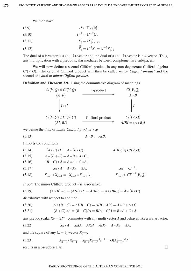
We then have

I2 ∈ F\0,(3.9)

I−1 = (I−2)I,(3.10)

Xk = 〈Xk〉n−k,(3.11) ˜Xk = I−2Xk = 〈I−2Xk〉k(3.12)

The dual of a k-vector is a (n− k)-vector and the dual of a (n− k)-vector is a k-vector. Thus,any multiplication with a pseudo scalar mediates between complementary subspaces.

We will now define a second Clifford product in any non-degenerate Clifford algebraCl(V,Q). The original Clifford product will then be called major Clifford product and thesecond one dual or minor Clifford product.

Definition and Theorem 3.9. Using the commutative diagram of mappings

Cl(V,Q)⊗Cl(V,Q)

(A ,B)∗-product

Cl(V,Q)

A∗B

I ⊗ I

I

Cl(V,Q)⊗Cl(V,Q)

(AI ,BI)Clifford product

Cl((V,Q)

AIBI = (A∗B)I

we define the dual or minor Clifford product ∗ as

A∗B := AIB.(3.13)

It meets the conditions

(A∗B)∗C = A∗ (B∗C), A,B,C ∈Cl(V,Q),(3.14)

A∗ (B+C) = A∗B+A∗C,(3.15)

(B+C)∗A = B∗A+C ∗A,(3.16)

Xn ∗A = A∗Xn = λA, Xn = λ I−1,(3.17)

Xn−1 ∗Xn−1 = 〈Xn−1 ∗Xn−1 〉n, Xn−1 ∈Cln−1(V,Q).(3.18)

Proof. The minor Clifford product ∗ is associative,

(A∗B)∗C = (AIB)∗C = AIBIC = A∗ (BIC) = A∗ (B∗C),(3.19)

distributive with respect to addition,

A∗ (B+C) = AI(B+C) = AIB+AIC = A∗B+A∗C,(3.20)

(B+C)∗A = (B+C)IA = BIA+CIA = B∗A+C ∗A,(3.21)

any pseudo scalar Xn = λ I−1 commutes with any multi vector A and behaves like a scalar factor,

Xn ∗A = XnIA = AXnI = AIXn = A∗Xn = λA,(3.22)

and the square of any (n−1)-vector Xn−1,

Xn−1 ∗Xn−1 = Xn−1Xn−1I4I−1 = Q(Xn−1)I4I−1(3.23)

results in a pseudo scalar.



Theorem 3.10. Let the set G(+, ·, ) endowed with the operations of addition (+), of scalarmultiplication (·) and of major Clifford multiplication (no sign) denote the Clifford F-algebraCl(V,Q) with non-degenerate quadratic form Q and decomposition into the direct sum of ho-mogeneous multi vector subspaces Clk(V,Q),

G =n⊕

k=0

Clk(V,Q).(3.24)

Let the set G(+, ·,∗) endowed with the operations of addition (+), of scalar multiplication (·)and of minor Clifford multiplication (∗) denote the Clifford F-algebra Cl(V , Q) with

V :=Cl(n−1)(V,Q),(3.25)

Q(X) := X ∗X = Q(X)I4I−1, X ∈ V , Q(X) ∈Cl0(V , Q) :=Cln(V,Q)(3.26)

and with decomposition into the direct sum of homogeneous multi vector subspaces Clk(V , Q),

G =n⊕

k=0

Clk(V , Q).(3.27)

The set G(+, ·, ,∗) endowed with the operations of addition (+), of scalar multiplication (·), ofmajor Clifford multiplication (no sign) and of minor Clifford multiplication (∗) represents anisomorphic Clifford double F-algebra.

Proof. We consider the decomposition of equation (3.24) as plus approach and the decomposi-tion of equation (3.27) as minus approach. By precondition F is a field with characteristic notequal to 2. The vector space V has dimension n,

dimV = dimCl(n−1)(V,Q) =

(n

n−1

)= n,(3.28)

and the mapping

Q : V =Cl1(V , Q) −→ F∼=Cl0(V , Q)(3.29)

is by definition of equation (3.26) a non-degenerate quadratic form on V . According to The-orem 3.9 the minor Clifford product ∗ is associative, distributive, has the identity element1− = (I+)−1 and coincides with scalar multiplication for all scalars X ∈Cl0(V , Q) in the minusapproach. The n homogeneous multi vectors

V E−i := Pi = (−1)i−1I−2P2

i P1 . . .Pi−1Pi+1 . . .Pn, i ∈ 1, . . . ,n=: L ⊂ N,(3.30)

form an orthogonal basis of and with respect to the inner product space (V , Q) and the 2n

homogeneous multi vectors

E−i1i2...ik :=

1− = (I+)−1 = 1+ k = 0 i1, i2, . . . , ik ⊂ LE−

i1 ∗E−i2 ∗ . . .∗E−

ik 0 < k ≤ n 1 ≤ i1 < i2 < · · ·< ik ≤ n(3.31)

= Pi1i2...ik

= (−1)−k(k+1)

2 +∑kl=1 il I−2

[k

∏l=1

P2il

]∏j∈M

Pj M := L \i1, i2, . . . , ik

=〈(−1)−k(k+1)

2 +∑kl=1 il I−2

[k

∏l=1

P2il

]∏j∈M

Pj〉+n−k



form a basis of the Clifford F-algebra Cl(V , Q) as a vector space. Thus, G(+, ·, ,∗) represents aClifford double F-algebra. G(+, ·, ,∗) represents even an isomorphic Clifford double F-algebrasince the linear mapping defined by

φ : Cl(V,Q) −→ Cl(V , Q)(3.32)

Pi −→ φ(Pi) := Ei

with

φ(λA+βB) = λφ(A)+βφ(B)(3.33)

φ(AB) = φ(A)∗φ(B)(3.34)

is an algebra-isomorphism.

Notation 3.11 (Clifford double algebra Γn). In section 6, the Clifford double F-algebra G(+, ·, ,∗)of Theorem 3.10 will be denoted by Γn(+, ·, ,∗).Definition 3.12 (inner and outer product in the minus approach). Let X−

kdenote the homoge-

neous multi vectors of the vector subspaces Clk(V , Q). The inner product in the minus approach

A−r B−

s := 〈A−r ∗B−

s 〉|r−s|, 0 ≤ r,s ≤ n,(3.35)

and the outer product in the minus approach

A−r ∨B−

s :=

0 r = 0 or s = 00 r+ s > n〈A−

r ∗B−s 〉r+s else

(3.36)

are defined in terms of the minor Clifford product and extended to generic multi vectors bydistributivity.

Corollary 3.13. The outer product ∨ of Cl(V , Q) is associative and has no identity element.

Corollary 3.14. Let G(+, ·,∗) represent the unital Clifford F-algebra Cl(V , Q) with the op-erations of addition (+), of scalar multiplication (·) and of minor Clifford multiplication (∗).The F-vector space G(+, ·) extended by the outer product ∨, i. e. the F-algebra G(+, ·,∨) isn-graded and has no identity element.

Theorem 3.15. Let Γn(+, ·, ,∗) be a non-degenerate, isomorphic Clifford double F-algebraand let G(+, ·,∧,∨) denote the F-vector space Γn(+, ·) extended by the two outer products ∧and ∨. G(+, ·,∧,∨) represents a complementary n-graded F-algebra.

Proof. According to Theorem 3.7 and Corollary 3.14 the F-algebras G(+, ·,∧) and G(+, ·,∨)with the decompositions G = ∑n

k=0 G+k = ∑n

k=0 G−k are n-graded. From equation (3.31) we get

G+k = G−

n−k for all k with 1 ≤ k ≤ n.

In section 6 we will generalize the concept of a double Clifford algebra Γn on the basisof projective algebra Λn to generic, i. e. also degenerate quadratic forms.

4. BINARY INDICES

Other authors have already used binary numbers to label elements of Clifford algebras invarious ways. See [Mar04] or [Lou01, p. 279ff]. We adopted the main idea and shortly reviewbinary numbers and several binary operators in this section.



Notation 4.1 (m-digit binary numbers). In order to label basis elements and other homogeneousmulti vectors we introduce binary numbers

(4.1) b ≡ bm−1 . . .b1b0 =

[m−1

∑k=0

bk2k

]10

, m ∈ N, bk ∈ 0,1,

with m digits bm−1, . . . , b0. The binary numbers will be noted by small latin letters in boldface, its m digits with the same letter but normal face and the digits will be numbered from 0 tom−1.

A m-digit number b translated into a real figure lies between [0]10 and [2m −1]10.

Definition 4.2 (sum of binary digits). The sum S(b) of the digits of the binary number (4.1) is

(4.2) S(b) :=

[n−1

∑k=0

bk

]10

.

Theorem 4.3. The m-digit binary number b

(a) is zero, if and only if S(b) = 0;(b) represents a decimal power of two, if and only if S(b) = 1;(c) is the decimal number [2m −1]10, if and only if S(b) = m.

Proof. (a) S(b) = 0 ⇔ bi = 0 ∀ 0 ≤ i ≤ m−1 ⇔ b = [0]2 = [0]10.(b) We have S(b) = 1, if and only if there is one index l ∈ N, such that the binary number

b = bm−1 . . .b1b0 bi =

1, if i = l,0, if i = l,(4.3)

= [2l]10, 0 ≤ l ≤ m−1,

represents a decimal power of two.(c) S(b) = m ⇔ bi = 1 ∀ 0 ≤ i ≤ m−1 ⇔ b = [2m −1]10.

Definition 4.4 (binary complement). The binary complement of a m-digit binary number b is

b = bm−1 . . .b1b0 :=

[m−1

∑k=0

bk2k

]10

with 0 := 1, 1 := 0.(4.4)

The binary complement translated into a decimal number lies again between [0]10 and[2n −1]10. In addition we always have

b+b = u = [2m −1]10,(4.5)

b = b,(4.6)

where u is the m-digit binary number with S(u) = m.

Definition 4.5 (indices on the left side). Let b be a m-digit binary number and I := i1, . . . , ikan ordered index set of length k with

0 ≤ i1 < i2 < .. . < ik ≤ m−1, k, j, i j ∈ N, 1 ≤ j ≤ k,(4.7)

such that

b = bm−1 . . .b1b0, bi =

1, if i ∈ I ,0, if i ∈ I .

(4.8)



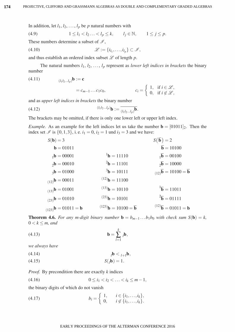
In addition, let l1, l2, . . . , lp be p natural numbers with

1 ≤ l1 < l2 . . . < lp ≤ k, l j ∈ N, 1 ≤ j ≤ p.(4.9)

These numbers determine a subset of I ,

L := il1 , . . . , ilp ⊂ I ,(4.10)

and thus establish an ordered index subset L of length p.

The natural numbers l1, l2, . . . , lp represent as lower left indices in brackets the binarynumber

b(l1l2...lp):= c(4.11)

= cm−1 . . .c1c0, ci =

1, if i ∈ L ,0, if i ∈ L ,

and as upper left indices in brackets the binary number

b(l1l2...lp) := b(l1l2...lp)

.(4.12)

The brackets may be omitted, if there is only one lower left or upper left index.

Example. As an example for the left indices let us take the number b = [01011]2. Then theindex set I is 0,1,3, i. e. i1 = 0, i2 = 1 und i3 = 3 and we have:

S(b) = 3 S(

b)= 2

b = 01011 b = 10100

b1 = 00001 b1 = 11110 b1 = 00100

b2 = 00010 b2 = 11101 b2 = 10000

b3 = 01000 b3 = 10111 b(12) = 10100 = b

b(12) = 00011 b(12) = 11100

b(13) = 01001 b(13) = 10110 b1= 11011

b(23) = 01010 b(23) = 10101 b2= 01111

b(123) = 01011 = b b(123) = 10100 = b b(12)= 01011 = b

Theorem 4.6. For any m-digit binary number b = bm−1 . . .b1b0 with check sum S(b) = k,0 < k ≤ m, and

b =k

∑l=1

bl ,(4.13)

we always have

bl < bl+1 ,(4.14)

S( bl ) = 1.(4.15)

Proof. By precondition there are exactly k indices

0 ≤ i1 < i2 < .. . < ik ≤ m−1,(4.16)

the binary digits of which do not vanish

bi =

1, i ∈ i1, . . . , ik,0, i ∈ i1, . . . , ik.(4.17)



Thus we have

b = bm−1 . . .b1b0 =

[k

∑l=1

2il

]10

=k

∑l=1

bl(4.18)

with bl = [2il ]10 and bl+1 = [2il+1 ]10., i. e. bl < bl+1 . The equation S(

bl)= 1 is a consequence

of Theorem 4.3. Notation 4.7 (nested sequence of left indices). For a binary number with several left indices,the nested sequence of left indices has to be read from inside outwards as in the followingexample,

bl4 (23) = 4

[l[

b(23)

]].(4.19)

Theorem 4.8. Let V be a vector space, Ai ∈V , i ∈ 1, . . . ,m ⊂N and b a binary variable withm digits. We may then label the m elements Ai with

V Ab, S(b) = 1,(4.20)

i. e. we use all binary numbers with S(b) = 1 to label the vectors Ab.

Proof. With bi =[2i−1]

10 we get S(bi) = 1 and Ai = Abi , 1 ≤ i ≤ m.

In this article we will also use the bitwise binary operators AND and XOR. Example:1001 AND 0101 = 0001 and 1001 XOR 0101 = 1100.

5. PROJECTIVE ALGEBRA Λn

Notation 5.1 (multiple outer product signs). The two outer products of projective algebra Λnare denoted by ∧ and ∨. For multiple outer products we use

m∧l=1

Xl := X1 ∧X2 ∧·· ·∧Xm,m∨

l=1

Xl := X1 ∨X2 ∨·· ·∨Xm.(5.1)

Definition 5.2 (projective algebra Λn). A projective F-algebra Λn(+, ·,∧,∨) is a set Λn withfour operations:

Λn ×Λn+−→ Λn

(A,B) −→ A+BF×Λn

·−→ Λn(α,A) −→ α ·A(5.2)

Λn ×Λn∧−→ Λn

(A,B) −→ A∧BΛn ×Λn

∨−→ Λn(A,B) −→ A∨B

(5.3)

The operations are called addition (+), scalar multiplication (no sign or ·), major outer product(∧) und minor outer product (∨). The obey the following conditions:

(P1) F is a field with char(F) = 2.(P2) The projective F-algebra Λn(+, ·,∧,∨) is a complementary n-graded F-algebra with de-

compositions into the direct sums

Λn =n⊕

k=0

Λk+n =

n⊕k=0

Λk−n , k,n ∈ N,(5.4)

and with the following dimensions for the whole algebra and for its subspaces,

dimΛn =n

∑k=0

dim(

Λkn

)=

n

∑k=0

(nk

), 0 ≤ k ≤ n.(5.5)

(P3) Further requirements for the outer products are:



• All scalars X0 ∈ Λ0n(+, ·) are left and right zero divisors,

X+0∧M = M∧X+

0= 0, ∀ M ∈ Λn,(5.6)

X−0∨M = M∨X−

0= 0, ∀ M ∈ Λn.(5.7)

In particular, the two algebras Λ+n and Λ−

n do not have an identity element.• For 1-vectors Ai ∈ Λ1+

n or Bi ∈ Λ1−n we have with l > 1

l∧i=1

Ai = 0 ⇐⇒

A1, A2, . . . , Al arelinearly independent.(5.8)

l∨i=1

Bi = 0 ⇐⇒

B1, B2, . . . , Bl arelinearly independent.(5.9)

Definition 5.3 (combined outer product). Any mathematical term which contains the combinedouter product ♦ can be read twice: Firstly with respect to the plus approach as major outerproduct ∧ and secondly with respect to the minus approach as minor outer product ∨.

Example. The expression

X1 ♦Y1 =−Y1 ♦X1 ∀ X1,Y1 ∈ Λ1n(5.10)

means

X+1∧Y+

1=−Y+

1∧X+

1∀ X+

1,Y+

1∈ Λ1+

n(5.11)

X−1∨Y−

1=−Y−

1∨X−

1∀ X−

1,Y−

1∈ Λ1−

n(5.12)

Notation 5.4 (multiple combined outer product sign). Analogous to the notation for multipleouter products we use for multiple combined outer products the sign

m

♦l=1

Xl := X1 ♦X2 ♦ · · ·♦Xm.(5.13)

Definition and Theorem 5.5 (basis of projective algebra in the plus approach). Let b be abinary variable with n digits, Pb with S(b) = 1 a set of n basis 1-vectors from Λ1+

n andP+

0 ∈ Λ0+n \0 a vector of grade 0. Then the homogeneous multi vectors

Pb :=

P+

0 , S(b) = 0,S(b)∧l=1

Pbl , 0 < S(b)≤ n,(5.14)

form a basis for the 2n-dimensional vector space of projective algebra Λn.

Definition and Theorem 5.6 (basis of projective algebra in the minus approach). Let b bea binary variable with n digits, Eb with S(b) = 1 a set of n basis 1-vectors from Λ1−

n andE−

0 ∈ Λ0−n \0 a vector of grade 0. Then the homogeneous multi vectors

Eb :=

E−

0 , S(b) = 0,S(b)∨l=1

E bl , 0 < S(b)≤ n,(5.15)

form a basis for the 2n-dimensional vector space of projective algebra Λn.

Notation 5.7 (basis n-vectors). For the n-vectors of the basis we also use the notation

I+ := P+b , I− := E−

b , S(b) = n.(5.16)

The superscript plus or minus sign can be omitted, if I stands for both approaches or if it isclear from the context in which approach one is working.



Notation 5.8 (basis of projective algebra). If an expression is true in the plus and in the minusapproache to projective algebra, the basis (5.14) and (5.15) are denoted by Bb, i. e. B+

b =Pb and B−

b = Eb.

Proof. In order to proof Theorem 5.5 and 5.6 we need to show that the 2n basis vectors Bbare linearly independent. According to Definition 5.2 homogeneous multi vectors of differentgrades are linearly independent. It remains to show, that homogeneous multi vectors Bb ofthe same grade S(b) = k are linearly independent. Trivially this is the case for S(b) = 0 andS(b) = n. The 1-vectors Bb are by precondition linearly independent. And for 2 ≤ S(b)≤ n−1we get with the coefficients λb ∈ F and with the binary n-digit numbers c

0 = ∑S(b)=k

λbBb(5.17)

⇐⇒ 0 =

[∑

S(b)=kλbBb

]♦Bc ∀ c with S(c) = k(5.18)

= ∑S(b)=k

λb (Bb ♦Bc)

= λc (Bc ♦Bc)

⇐⇒ 0 = λc, ∀ c with S(c) = k.(5.19)

The sets Pb and Eb both form a basis for the same 2n-dimensional vector spaceΛn(+, ·). This is why there is always a regular transformation changing the vectors of one basisinto the vectors of the other basis.

Notation 5.9 (basis transformation). Let ζbc denote the basis transformation with which wecan express the basis vectors of Eb in terms of the basis vectors of Pb,

Eb = ∑S(c)=n−k

ζbcPc, 0 ≤ S(b) = k ≤ n,(5.20)

and let ζ−1bc denote the inverse basis transformation with which we can express the basis vectors

of Pb in terms of the basis vectors of EbPb = ∑

S(c)=n−kζ−1

bc Ec, 0 ≤ S(b) = k ≤ n,(5.21)

where b and c represent n-digit binary numbers.

We then get with the n-digit binary number d with S(b) = S(d) = k

∑S(c)=n−k

ζbcζ−1cd = ∑

S(c)=n−kζ−1

bc ζcd = δbd,(5.22)

where δbd is the Kronecker-delta-symbol,

δbd :=

1, b = d,0, b = d.(5.23)

By means of the basis transformation ζbc it is now possible to compute the major outerproduct ∧ also in the minus approach and the minor outer product ∨ also in the plus approach.Thus, the two outer products of the projective algebra Λn(+, ·,∧,∨) are available for any multivectors of the algebra.



Theorem 5.10. Let b,c,d and e be binary n-digit numbers with

d = b AND c(5.24)e = b XOR c(5.25)

Then we have

Bb ♦Bc =

αbcBe, S(d) = 0, S(b) = 0, S(c) = 0,0, S(d) = 0,0, S(b) = 0 or S(c) = 0,

(5.26)

with the coefficients

αbc = (−1)∑n−1l=1 bl ∑l−1

m=0 cm = (−1)∑n−2l=0 cl ∑n−1

m=l+1 bm .(5.27)

Proof. We determine two sequences of transpositions such that the factors, i. e. the 1-vectors ofthe outer product Bb♦Bc get in an order where equal 1-vectors are direct neighbors. We depictthe order of 1-vectors in the product Bb ♦Bc by

(b0b1 . . .bn−2bn−1)(c0c1 . . .cn−2cn−1).(5.28)

First sequence of transpositions: We move the 1-vectors of Bc and shift them in terms oftranspositions from the right side to the left side. Take first c0 and shift it to the left side until itstands between b0 and b1, then take c1 and shift it to the left side until it stands between b1 andb2 and so forth. The last transposition of this first sequence is then the shift of cn−2 to the leftside such that it stands between bn−2 and bn−1. The resulting order of the 1-vectors

(b0c0b1c1 . . .bn−2cn−2bn−1cn−1)(5.29)

was achieved by altogethern−2

∑l=0

cl

n−1

∑m=l+1

bm(5.30)

transpositions.

Second sequence of transpositions: We move the 1-vectors of Bb and shift them in termsof transpositions from the left side to the right side. Take first bn−1 and shift it to the right sideuntil it stands between cn−2 and cn−1, then take bn−2 and shift it to the right side until it standsbetween cn−3 and cn−2 and so forth. The last transposition of this second sequence is then theshift of b1 to the right side such that it stands between c0 and c1. The resulting order of the1-vectors

(b0c0b1c1 . . .bn−2cn−2bn−1cn−1).(5.31)

was achieved by altogethern−1

∑l=1

bl

l−1

∑m=0

cm(5.32)

transpositions.

In both sequences the number of transpositions is the samen−2

∑l=0

cl

n−1

∑m=l+1

bm =n−1

∑l=1

bl

l−1

∑m=0

cm.(5.33)

The outer product Bb♦Bc vanishes if and only if there is at least one pair (bl,cl), 0 ≤ l ≤n−1, with blcl = 1, i. e. if and only if S(d) = 0.



Corollary 5.11. Let b be a n-digit binary number with S(b) = 0 and S(b) = n. Then we have

Bb ♦Bb =

αbb I S(b) = 0 and S(b) = n0 S(b) = 0 or S(b) = n(5.34)

Proof. It is a consequence of Theorem 5.10 with c = b.

Theorem 5.12. Let b and c be n-digit binary numbers. We then have

αbcαcb = (−1)S(b)S(c)−S(bANDc)(5.35)

Proof.

αbcαcb = (−1)∑n−2l=0 cl ∑n−1

m=l+1 bm+∑n−1l=1 cl ∑l−1

m=0 bm(5.36)

= (−1)c0 ∑n−1m=1 bm+∑n−2

l=1 cl[∑n−1m=l+1 bm+∑l−1

m=0 bm]+cn−1 ∑n−2m=0 bm

= (−1)c0S(b)+S(b)∑n−2l=1 cl+cn−1S(b)−[c0b0+∑n−2

l=1 clbl+cn−1bn−1]

= (−1)S(b)S(c)−S(bANDc)

Theorem 5.13. For homogeneous multi vectors of grade r and s we have,

Xr ♦Ys = (−1)rs ·Ys ♦Xr.(5.37)

Proof. Let b and c be n-digit binary numbers with sum of digits S(b) = r and S(c) = s. Thenthere are coefficients λb and µc such that

Xr ♦Ys =

[∑

S(b)=rλbBb

]♦[

∑S(c)=s

µcBc

](5.38)

= ∑S(b) = rS(c) = s

λbµc ·Bb ♦Bc

= ∑S(b) = rS(c) = s

λbµc ·αbcαcb Bc ♦Bb

= ∑S(b) = rS(c) = s

(−1)rsλbµc ·Bc ♦Bb

= (−1)rs ·[

∑S(c)=s

µcBc

]♦[

∑S(b)=r

λbBb

]= (−1)rs ·Ys ♦Xr.

where we used Theorem 5.12 in the step from the third to the fourth line.

Definition 5.14 (harmonic model of projective algebra). Let b and c be n-digit binary numbers.The harmonic model of projective algebra Λn is determined by the basis transformation

ζbc := αbbδcb.(5.39)

Since αbbδcb is a regular transformation, the harmonic model of projective algebra iswell defined.



Theorem 5.15. In the harmonic model of projective algebra we have

Eb = αbbPb ⇐⇒ Pb = αbbEb, 0 ≤ S(b)≤ n,(5.40)

with

αbb = (−1)∑n−2l=0 bl ∑n−1

m=l+1 bm = (−1)∑n−1l=1 bl ∑l−1

m=0 bm ,(5.41)

αbb = (−1)k(n−k)αbb.(5.42)

Proof. Insert equation (5.39) into equation (5.20).

Theorem 5.16. In the harmonic model of projective algebra we have for the k-vectors

X+k= ∑

S(b)=kµbPb, Y−

k= ∑

S(b)=kνbEb, 0 < k < n,(5.43)

the two equivalent equations

X+k∧Y−

k=

[∑

S(b)=kµbνb

]I+ ⇔ X+

k∨Y−

k=

[∑

S(b)=kµbνb

]I−.(5.44)

Proof.

X+k∧Y−

k=

[∑

S(b)=kµbνb

]I+(5.45)

⇐⇒ ζbc = αbb δcb

⇐⇒ ζ−1cb = αbb δbc

⇐⇒ X+k∨Y−

k=

[∑

S(b)=kµbνb

]I−

The harmonic model of projective algebra is strongly related to what HANNS-JORGSTOSS calls Harmonisches Punkt-Geraden-System [Sto09, Bezeichnung 2.21 on p. 29] andmore general Harmonisches Punkt-Hyperebenen-System [Sto09, Bezeichnung 3.36 on p. 51].

6. CLIFFORD DOUBLE ALGEBRA Γn

Definition 6.1 (symmetric bilinear forms). Let

b : Λ1n ⊗Λ1

n −→ Λ0n

(X ,Y ) −→ b(X ,Y ) = b(Y,X)(6.1)

be two symmetric bilinear forms, one in the plus, the other in the minus approach of projectivealgebra Λn.

Notation 6.2 (multiple Clifford product signs). The two Clifford products of double Cliffordalgebra Γn are denoted by ‘no sign’ and ∗. For multiple Clifford products we use

m

∏l=1

Xl := X1X2 · · ·Xm,m∗

l=1Xl := X1 ∗X2 ∗ · · · ∗Xm.(6.2)



Definition 6.3 (orthogonal basis). Let Λn(+, ·,∧,∨) be a projective F-algebra. A basis Bbof Λn is called an orthogonal basis, if and only if the set of all 1-vectors

O := Bb | S(b) = 1(6.3)

is a system of orthogonal vectors with respect to the bilinear form b,

b(Bb,Bb1) = 0 for all b = b1 with Bb,Bb1 ∈ O.(6.4)

Definition 6.4 (Clifford double algebra Γn). Let Λn(+, ·,∧,∨) be a projective F-algebra andlet b denote two symmetric bilinear forms according to equation (6.1). A Clifford double F-algebra Γn(+, ·,∧,∨, ,∗) is the projective algebra Λn(+, ·,∧,∨) extended by the operations

Λn ×Λn −→ Λn(A,B) −→ AB

Λn ×Λn∗−→ Λn

(A,B) −→ A∗B(6.5)

called major Clifford product (no sign) and minor Clifford product (∗). The Clifford productsobey the following conditions:

(C1) They are associative and distributive,

(AB)C = A(BC), A,B,C ∈ Λn,(6.6)

A(B+C) = AB+AC, (A+B)C = AC+BC,(6.7)

(A∗B)∗C = A∗ (B∗C),(6.8)

A∗ (B+C) = A∗B+A∗C, (A+B)∗C = A∗C+B∗C.(6.9)

(C2) If at least one factor is a scalar X0 = α1, α ∈ F, the Clifford products reduce to scalarmultiplication,

X+0

M = MX+0= αM, ∀ X+

0∈ Λ0+

n , ∀ M ∈ Λn,(6.10)

X−0∗M = M ∗X−

0= αM, ∀ X−

0∈ Λ0−

n , ∀ M ∈ Λn.(6.11)

(C3) Contraction rule for the 1-vectors.

X+1

X+1= b+(X+

1,X+

1) ∈ Λ0+

n ∀ X+1∈ Λ1+

n(6.12)

X−1∗X−

1= b−(X−

1,X−

1) ∈ Λ0−

n ∀ X−1∈ Λ1−

n(6.13)

(C4) For an orthogonal set O = X1,X2, . . . ,Xm ⊂ Λ1n of m homogeneous multi vectors of

grade 1 the Clifford and outer products are the same,m

∏l=1

Xl =m∧

l=1

Xl ⇐⇒

O+ is a orthogonal system withrespect to the bilinear form b+.

(6.14)

m∗l=1

Xl =m∨

l=1

Xl ⇐⇒

O− is a orthogonal system withrespect to the bilinear form b−.(6.15)

Definition 6.5 (combined Clifford product). Any mathematical term which contains the com-bined Clifford product can be read twice: Firstly with respect to the plus approach as majorClifford product (no sign) and secondly with respect to the minus approach as minor Cliffordproduct ∗.

Notation 6.6 (multiple combined Clifford product sign). For the multiple combined Cliffordproduct we use the sign

ml=1

Xl := X1 X2 · · ·Xm.(6.16)



Definition 6.4 of a Clifford double algebra Γn(+, ·,∧,∨, ,∗) coincides in the case of anon-degenerate quadratic form

Q(X) := b(X ,X), X ∈ Γ1n,(6.17)

with the Clifford double algebra mentioned in Theorem 3.10 and Notation 3.11. Compared toTheorem 3.10 the Definition 6.4 of a Clifford double algebra is more general, since it includesClifford double algebras with a degenerate quadratic form Q. This is why we regard Definition6.4 as the standard definition of a Clifford double algebra.

Theorem 6.7. Let Bb be an orthogonal basis of the Clifford double F-algebra Γn(+, ·,∧,∨, ,∗).We then have

Bb = B0 ∈ Γ0n, S(b) = 0,(6.18)

Bb =S(b)l=1

B bl ∈ ΓS(b)n , 1 ≤ S(b)≤ n.(6.19)

Proof. The proposition follows immediately from equations (5.14), (5.15), (6.14) and (6.15).

Theorem 6.8. Let Bb be an orthogonal basis of Γn(+, ·,∧,∨, ,∗) and the variables b,c,d,eand u n-digit binary numbers with

d = b AND c,(6.20)e = b XOR c,(6.21)

S(u) = n.(6.22)

We then have

Bb Bc =

BbBc,

S(b) = 0orS(c) = 0,

αbcBe,

S(d) = 0,S(b) = 0,S(c) = 0,

αbc

[∏S(d)

p=1b(B dp ,B dp )]

Be, S(d)> 0,

(6.23)

with

S(b)+S(c) = 2 ·S(d)+S(e)(6.24)

0 ≤ |S(b)−S(c)| ≤ S(e)≤ Dn(S(b)+S(c))≤ n(6.25)

Dn(i) =

i 0 ≤ i ≤ n2n− i n < i ≤ 2n(6.26)

and in the special case c = u and I = Bu

Bb I = (−1)S(b)(n−1)I Bb(6.27)

=

αbuBb S(d) = 0,αbu

[∏S(b)

p=1b(B bp ,B bp )]

Bb, S(d)> 0,

Proof. According to the proof of Theorem 5.10 we needn−1

∑l=1

bl

l−1

∑m=0

cm =n−2

∑l=0

cl

n−1

∑m=l+1

bm(6.28)



transpositions, in order to bring the 1-vectors of BbBc into such an order that equal 1-vectorsare standing side by side. This is how we get the coefficient αbc in equation (6.23). Thereare S(d) 1-vectors P bp , which show up twice in the product Bb Bc and where the Cliffordproduct reduces according to the contraction rule (6.12) or (6.13) to the scalar b(P bp ,P bp ). Theremaining 1-vectors are collected in the homogeneous multi vector Be. Thus equation (6.23) istrue.

The S(b)+S(c) 1-vectors of the product BbBc contain S(d) pairs of identical 1-vectors.This is why the homogeneous multi vector Be is made up of exactly S(b)+ S(c)− 2 · S(d) 1-vectors. This is equivalent to equation (6.24).

The lower limit for S(e) in equation (6.25) is realised, if all S(b) 1-vectors of Bb showup in Bc or if all S(c) 1-vectors of Bc show up in Bb. The upper limit for S(e) in equation(6.25), i. e. the expression of equation (6.26) becomes clear, if we consider that there are atmost n different 1-vectors. So, if the sum S(b)+ S(c) is bigger than n, there must be at leastS(b)+S(c)−n pairs of identical 1-vectors.

Inserting c = u in equation (6.23) we get the special case of equation (6.27). Theorem 6.9. For the Clifford product between the homogeneous multi vectors Xr and Ys weget

Xr Ys =m

∑k=0

〈Xr Ys〉|r−s|+2k(6.29)

with

m =Dn(r+ s)−|r− s|

2,(6.30)

and the index function Dn of equation (6.26).

Proof. We can write the homogeneous multi vectors Xr und Ys as linear combinations withrespect to the basis Bb,

Xr = ∑S(b)=r

µbBb,(6.31)

Ys = ∑S(c)=s

νcBc,(6.32)

an then get

Xr Ys = ∑S(b) = rS(c) = s

µbνc Bb Bc.(6.33)

According to Theorem 6.8, the grades of the product Bb Bc lie between |r− s| and Dn(r+ s)and differ by a multiple of 2 from the limits |r − s| or Dn(r + s), since, if there are identicalpairs present in the product Bb Bc, always two 1-vectors disappear.

We are now in the position to compute the Clifford product of any two generic multivectors M and N,

MN =n

∑r,s=0

〈M〉r 〈N〉s, M,N ∈ Γn.(6.34)

Theorem 6.10. For the homogeneous multi vectors Xr and Ys we have

Xr ♦Ys =

〈Xr Ys〉r+s, r+ s ≤ n, r = 0, s = 00, else.(6.35)



Proof. For r+ s > n, r = 0 or s = 0 the outer product ♦ vanishes. In the cases r+ s ≤ n, r = 0and s = 0 the outer product Xr ♦Ys has not to vanish. Using the equations (6.33), (6.23) and(5.26) we get

〈Xr Ys〉r+s = ∑S(b) = rS(c) = s

µbνc 〈Bb Bc〉r+s = ∑S(b) = rS(c) = s

µbνc 〈αbcBbXORc〉r+s(6.36)

= ∑S(b) = rS(c) = s

µbνc Bb ♦Bc = Xr ♦Ys.

Definition 6.11 (inner products). Let Γn(+, ·,∧,∨, ,∗) be a Clifford double F-algebra. Theoperations

Λn ×Λn·−→ Λn

(A,B) −→ A ·BΛn ×Λn

−→ Λn(A,B) −→ AB

(6.37)

are called major inner product (·) and minor inner product () and obey the following condi-tions:

Xr ·Ys := 〈XrYs〉|r−s|, Xr ∈ Γr+n , Ys ∈ Γs+

n ,(6.38)

Xr Ys := 〈Yr ∗Xs〉|r−s| Xr ∈ Γr−n , Ys ∈ Γs−

n ,(6.39)

A · (B+C) = A ·B+A ·C, A,B,C ∈ Γn,(6.40)

(A+B) ·C = A ·C+B ·C,(6.41)

A (B+C) = AB+AC,(6.42)

(A+B)C = AC+BC.(6.43)

Definition 6.12 (combined inner product). Any mathematical term which contains the com-bined inner product can be read twice: Firstly with respect to the plus approach as majorinner product · and secondly with respect to the minus approach as minor inner product .

The inner product is well defined in Definition 6.11 since the Clifford product isalso distributive.

Theorem 6.13. In the case r = 0 or s = 0 the inner product and the scalar multiplication arethe same,

Ar Bs = Ar Bs = ArBs, r = 0 or s = 0.(6.44)

Proof. Compare equations (6.10) or (6.11) with Definition 6.11. Theorem 6.14. For homogeneous multi vectors of grade r and s with r ≥ s we have,

Xr Ys = (−1)s(r−1)Ys Xr.(6.45)

Proof. Let b and c be n-digit binary numbers with sum of digits S(b) = r and S(c) = s. Thenthere are coefficients λb and µc such that

Xr Ys =〈[∑

S(b)=rλbBb

][

∑S(c)=s

µcBc

]〉r−s

(6.46)

=〈 ∑S(b) = rS(c) = s

λbµc ·Bb Bc〉r−s



=〈 ∑S(b) = rS(c) = s

λbµc ·αbcαcb Bc Bb〉r−s

=〈 ∑S(b) = rS(c) = s

(−1)rs−sλbµc ·Bc Bb〉r−s

=〈(−1)rs−s ·[

∑S(c)=s

µcBc

][

∑S(b)=r

λbBb

]〉r−s

= (−1)s(r−1) ·Ys Xr.

where we used equation (5.35) for the step from the third to the fourth line. Theorem 6.15. For 1-vectors X and Y we have

X Y = X Y +X ♦Y, X ,Y ∈ Γ1n,(6.47)

where the inner product is symmetric and the outer product is antisymmetric. The inner productis given by

X Y = b(X ,Y ), X ,Y ∈ Γ1n.(6.48)

Proof. Equation (6.47) is a consequence of Theorem 6.9. According to equation (5.37) theouter product between two 1-vectors is antisymmetric and according to equation (6.45) the in-ner product between two 1-vectors is symmetric. With X = ∑S(b)=1 λbBb and Y = ∑S(c)=1 µcBcwe get equation (6.48),

X Y = ∑S(b)=1

λbµbb(Bb,Bb)(6.49)

= b

(∑

S(b)=1λbBb , ∑

S(c)=1µcBc

)= b(X ,Y ).

Theorem 6.16. Let Γn be a Clifford double F-algebra, let Bb be the orthogonal bases in thetwo approaches and let

φ : Γ+n −→ Γ−

n(6.50)

Pb −→ φ(Pb) := Eb

with

φ(A∧B) := φ(A)∨φ(B)(6.51)

represent an algebra isomorphism mapping the plus approach Λn(+, ·,∧) onto the minus ap-proach Λn(+, ·,∨). The isomorphism φ preserves the Clifford products

φ(AB) = φ(A)∗φ(B), A,B ∈ Γn,(6.52)

if and only if it preserves the bilinear forms

φ(b+(X ,Y )) = b−(φ(X),φ(Y )), X ,Y ∈ Γ1+n .(6.53)

Proof.

φ(AB) = φ(A)∗φ(B), A,B ∈ Γn,

⇐⇒ φ(XY ) = φ(X)∗φ(Y ), X ,Y ∈ Γ1+n ,



⇐⇒ φ(X ·Y )+φ(X ∧Y ) = φ(X)φ(Y )+φ(X)∨φ(Y ),⇐⇒ φ(X ·Y ) = φ(X)φ(Y ),⇐⇒ φ(b+(X ,Y )) = b−(φ(X),φ(Y )).

With Theorem 6.16 we know, that a generic Clifford double F-algebra Γn does not needto be isomorphic.

Theorem 6.17. Let Γn be a Clifford double F-algebra with

b(X ,Y ) = 0 for all X ,Y ∈ Γ1n.(6.54)

In this case Γn represents a Grassmann double F-algebra, i. e. Γ+n (+, ·, ) and Γ−

n (+, ·,∗) areboth Grassmann algebras.

Proof. According to equations (6.10) and (6.11) of Definition 6.4 there is an identity elementin both approaches. With the vanishing bilinear form of equation (6.54) we have

Xr Ys = Xr ♦Ys for all r = 0,s = 0.(6.55)

7. GRASSMANN ALGEBRAS

Since projective and Grassmann algebra look very similar, let us compare the two struc-tures. A Grassmann algebra

∧V of a vector space V with dimV = n is an associative, unital,

graded and antisymmetric algebra of dimension 2n. Projective algebra Λn is a double n-gradedalgebra, this is why we can only check whether the plus approach Λn(+, ·,∧) or the minusapproach Λn(+, ·,∨) show the structure of a Grassmann algebra.

There is no difference between the algebras Λn(+, ·,∧), Λn(+, ·,∨) and∧

V inasmuch asthey are all associative, graded, antisymmetric and inasmuch as they have the same dimensionson the level of the whole algebra as well as on the level of their subspaces. The differencebetween the algebras Λn(+, ·,∧), Λn(+, ·,∨) and

∧V is that there is no identity element present

in projective algebra — all scalars are zero divisors — and the Grassmann algebra is unital.

John Browne used the term Grassmann algebra in [Bro12] to describe the body of al-gebraic theory and results based on Graßmann’s Ausdehnungslehre from 1844 and from 1862.This form of Grassmann algebra is very similar to projective algebra and Clifford double alge-bra. We will now compare the approach of John Browne with an appropriate Clifford doublealgebra.

To do this we use two colums. On the left side you will find the concepts and notationsfrom John Brownes book Grassmann algebra. Volume 1: Foundations [Bro12]. On the rightside we enlist the corresponding concepts in the language of Clifford double algebra.

John Browne’s Grassmann algebra

Grassmann algebra: [Λ :=]⊕n

k=0 Λk

dim

(n⊕

k=0Λk

)=

n

∑k=0

dim Λk=

n

∑k=0

(nk

)= 2n

Operations in the Grassmann algebra:

Clifford double algebra

Grassmann algebra: plus approach of Γn witha bilinear form b(X ,Y ) = 0 as in eq. (6.54).

dimΓn =n

∑k=0

dimΓkn =

n

∑k=0

(nk

)= 2n

Operations in the Grassmann algebra Γn:



• addition (+)• scalar multiplication (no sign)• exterior product (∧)• regressive product (∨)

Λ(+, ,∧) and Λ(+, ,∨) are both Grassmannalgebras.

Identity element 1=10∈ Λ(+, ,∧)

Identity element 1n∈ Λ(+, ,∨)

Common factor axiom and theorem

To be continued ...

• addition (+)• scalar multiplication (·)• major outer product (no sign)• minor outer product (∗)

Γ+n (+, ·, ) and Γ+

n (+, ·,∗) with a bilinear formb(X ,Y ) = 0 as in eq. (6.54) are both Grass-mann algebras.

Identity element 1+ ∈ Γ+n (+, ·, )

Identity element 〈1−〉+ ∈ Γ+n (+, ·,∗)

Basis transformation ζbc

...

8. OUTLOOK

Projective algebra Λn and double Clifford algebra Γn may be applied in the field of ge-ometry. A system of axioms for the 2n-dimensional projective geometry is given in terms ofprojective algebra Λn in [Con16]. Cayley-Klein geometries can be expressed in terms of doubleClifford algebra Γn. See [Con00],[Con08, Chapter 5] and [Gun11]. In both cases the structureof a double graded algebra is needed to incorporate the projective principle of duality, whichis present in projective geometry as well as in the non-degenerate Cayley-Klein geometries.[Kow09]

Because of the deep geometric significance of projective and double Clifford algebra, weclose this article with

Definition 8.1 (geometric algebra). The term geometric algebra is used for projective algebraΛn and for double Clifford algebra Γn.

REFERENCES

[Bro12] J. BROWNE, Grassmann Algebra. Volume 1: Foundations. Exploring extended vector algebra withMathematica, Barnard Publishing, Eltham, Australia, 2012.

[Con00] O. CONRADT, The principle of duality in clifford algebra and projective geometry, in Clifford Alge-bras and their Applications in Mathematical Physics (R. ABŁAMOWICZ and B. FAUSER, eds.), 1,Birkhauser, 2000, pp. 157–194.

[Con08] O. CONRADT, Mathematical Physics in Space and Counterspace, 2nd ed., Verlag am Goetheanum,Dornach, 2008.

[Con16] O. CONRADT, Projective geometry with projective algebra, in ???, 2016.[Gun11] C. GUNN, Geometry, Kinematics, and Rigid Body Mechanics in Cayley-Klein Geometries, Ph.D. thesis,

Technische Universitat Berlin, Berlin, September 2011.[HZ91] D. HESTENES and R. ZIEGLER, Projective geometry with clifford algebra, Acta Appl. Math. 23 (1991),

25–63.[Kow09] G. KOWOL, Projektive Geometrie und Cayley-Klein Geometrien der Ebene, Birkauser, Basel, Boston,

Berlin, 2009.[Lou01] P. LOUNESTO, Clifford Algebras and Spinors, second ed., London Mathematical Society Lecture Note

Series 286, Cambridge University Press, Cambridge, 2001.[Mar04] D. W. MARKS, A binary index notation for clifford algebras, in Clifford Algebras. Applications to

Mathematics, Physics, and Engineering (R. ABŁAMOWICZ, ed.), Progress in Mathematical Physics34, Birkhauser, Boston, Basel, Berlin, 2004, pp. 343–350.

[Sto09] H.-J. STOSS, Koordinaten im projektiven Raum, Mathematisch-Astronomische Blatter. Neue Folge 27,Verlag am Goetheanum, Dornach, 2009.



PROJECTIVE GEOMETRY WITH PROJECTIVE ALGEBRA(PRELIMINARY VERSION)

Oliver Conradt a

a Section for Mathematics and AstronomyGoetheanum, Ruttiweg 45, CH 4143 Dornach, Switzerland.


ABSTRACT. This article provides a system of axioms for projective geometry Pn in termsof projective algebra Λn. Basic concepts of projective geometry Pn such as the principle ofduality, primitive geometric forms, the cross ratio of four basic elements and simple projectivetransformations are then determined on the base of the above mentioned system of axioms.

1. INTRODUCTION

After the discovery of the principle of duality by the French mathematicians JEAN VIC-TOR PONCELET (1788-1867) and JOSEPH-DIAZ GERGONNE (1771-1859) in the first quarterof the nineteenth century projective geometry experienced an impulse of development for aboutone century. This impulse expressed itself in a synthetic as well as in an analytic form. In thecourse of the twentieth century the synthetic approach became less and less known althoughsynthetic projective geometry had led to a wealth of new concepts and an unsurpassed beauty.An example for the new concepts rising out of synthetic projective geometry is the notion ofcounterspace [Con08, pp. 55].

Nevertheless, the synthetic approach to projective geometry was further developed inthe twentieth century by authors like e. g. OSWALD VEBLEN (1880-1960) [VY10, Veb18],GEORGE ADAMS (1894-1963) [Ada65], LOUIS LOCHER (1906-1962) [Loc80b, Loc80a, Loc70b,Loc70a], HAROLD SCOTT MACDONALD COXETER (1907-2003) [Cox74], LAWRENCE ED-WARDS (1912-2004) [Edw03], HANNS-JORG STOSS [Sto95, Sto99], GERHARD KOWOL [Kow09]and RENATUS ZIEGLER [Zie12].

The purpose of this paper is to provide a system of axioms for projective geometry Pnin terms of projective algebra Λn [Con16]. The aim thereby was to analytically represent intoevery detail the wealth of synthetic projective geometry as it is described e. g. in the books byLOUIS LOCHER [Loc80b, Loc80a, Loc70b].

Section 2 introduces the system of axioms for projective geometry Pn in terms of pro-jective algebra Λn. The sections 3-6 provide basic concepts of projective algebra Pn such asthe principle of duality, primitive geometric forms, the cross ratio of four basic elements andsimple projective transformations.

This paper uses the concepts, notations, definitions and theorems given in [Con16] with-out repeating them here again.

2. A SYSTEM OF AXIOMS FOR PROJECTIVE GEOMETRY Pn

Definition 2.1 (equivalence relation). Two multi vectors A and B of a projective F-algebra Λnare called equivalent, if and only if A and B differ in a number ξ ∈ F\0,

A B :⇐⇒ A = ξ B.(2.1)

Date: July 22, 2016.

188


Definition 2.2 (projective geometry Pn). Let Λn(+, ·,∧,∨) be a projective F-algebra. Pro-jective geometry Pn of dimension 2n is determined in terms of projective algebra Λn by thefollowing axioms:

(A1) Elements of projective geometry.(a) There are n+1 different types of basic elements corresponding to the n+1 different

vector subspaces Λkn of projective algebra Λn. The basic elements of a certain type

(called k-elements) are represented by the homogeneous multi vectors Xk of one ofthe n+1 different vector subspaces Λk

n.(b) A multi vector M of the vector space Λn(+, ) represents an element, i. e. in general

of each type of basic element exactly one.

M =n

∑k=0

〈M〉k.(2.2)

(c) Equivalent multi vectors represent the same geometric element.(A2) Incidence relation. Two elements A und B are incident if and only if the corresponding

multi vectors A and B meet the conditions

A∧B = 0 and A∨B = 0.(2.3)

(A3) Intersection and connection. The geometric operation of connection corresponds to themajor outer product (∧), the geometric operation of intersection to the minor outer prod-uct (∨).

Definition 2.3 (real, complex or finite projective geometry). Depending on the field F of theprojective F-algbera Λn we have a) for F = R real projective geometry, b) for F = C complexprojective geometry and c) for finite F finite projective geometry.

Definition 2.4 (names of basic elements). In case of the projective geometries P2, P3 and P4we use the in Table 1 listed names for the different types of basic elements.

Definition 2.5 (space and counterspace). Inasmuch as projective geometry Pn is expressed interms of the plus approach Λ+

n it is called space and inasmuch as it is expressed in terms of theminus approach Λ−

n it is called counterspace.

Remark 2.6. The terms space and counterspace are in a similar way also used in the Cayley-Klein geometries. The Cayley-Klein geometries may be expressend in terms of double Cliffordalgebra Γn [Con16]. And again, the plus approach is called space and the minus approachcounterspace in these metric geometries.

3. PRINCIPLE OF DUALITY

Definition 3.1 (major dual). The major dual S′ of any expression S from projective geometryPn such as e. g. an equation, a theorem, or a definition is obtained by interchanging ∧ with ∨and by reversing the sign of the plus-minus notation.

Theorem 3.2 (major principle of duality). Any statement S from projective geometry Pn is trueif and only if the major dual statement S′ from projective geometry Pn is true.

Proof. According to Theorem 5.14 of [Con16] projective algebra Λn is a double n-graded al-gebra, i. e. there is always an isomorphism between Λ+

n and Λ−n .

Definition 3.3 (minor dual). The minor dual S′′ of any expression S from projective geometryPn such as e. g. an equation, a theorem, or a definition is obtained by interchanging ∧ with ∨and by replacing the grades of a multi vector with the complementary grades (k → n− k).

PROJECTIVE GEOMETRY WITH PROJECTIVE ALGEBRA 189


P2 lineΛ0+

2 = Λ2−2 line

Λ1+2 = Λ1−

2 points or planesΛ2+

2 = Λ0−2 line

P2 incident point-plane-pairΛ0+

2 = Λ2−2 incident point-plane-pair

Λ1+2 = Λ1−

2 linesΛ2+

2 = Λ0−2 incident point-plane-pair

P3 planar fieldΛ0+

3 = Λ3−3 field of lines as such

Λ1+3 = Λ2−

3 pointsΛ2+

3 = Λ1−3 lines

Λ3+3 = Λ0−

3 field of points as suchP3 centric bundle

Λ0+3 = Λ3−

3 bundle of planes as suchΛ1+

3 = Λ2−3 lines

Λ2+3 = Λ1−

3 planesΛ3+

3 = Λ0−3 bundle of lines as such

P4 spaceΛ0+

4 = Λ4−4 space of planes as such

Λ1+4 = Λ3−

4 pointsΛ2+

4 = Λ2−4 linear complexes (including the lines)

Λ3+4 = Λ1−

4 planesΛ4+

4 = Λ0−4 space of points as such

TABLE 1. The names for the different types of basic elements in the projectivegeometries P2, P3 and P4.

Space Λ+n Counterspace Λ−

n

X+k

↔ X−k∧ ↔ ∨

∨ ↔ ∧A∧B = 0

andA∨B = 0

↔ A∨B = 0

andA∧B = 0

TABLE 2. Major principle of duality in projective geometry Pn.

Theorem 3.4 (minor principle of duality). Any statement S from projective geometry Pn istrue if and only if the minor dual statement S′′ from projective geometry Pn is true.

Proof. S ⇐⇒ S′ ⇐⇒ S′′

4. PRIMITIVE GEOMETRIC FORM

Definition 4.1 (k-primitive geometric form of grade m). Let Xi = 〈Xi〉k denote m+ 1 linearindependent k-vectors in projective geometry Pn with 1 ≤ i ≤ m+ 1 ≤ (n

k

)and 0 ≤ k ≤ n.

PROJECTIVE GEOMETRY WITH PROJECTIVE ALGEBRA190


Space Λ+n Space Λ+

nCounterspace Λ−

n Counterspace Λ−n

Xk ↔ Xn−k∧ ↔ ∨

A∧B = 0and

A∨B = 0

↔ A∨B = 0

andA∧B = 0

TABLE 3. Minor principle of duality in projective geometry Pn.

Then the k-primitive geometric form of grade m is the sub vector space

U :=

m+1

∑i=1

ξiXi

∣∣∣∣∣ξi ∈ F

(4.1)

of projective algebra Λn with dimU = m+1.

The Tables 4 and 5 list all primitive geometric forms of the projective geometries P2,P3 and P4.

Definition 4.2 (general position of l basic elements). Let L := i | i, l ∈ N,1 ≤ i ≤ l be theset of the l first natural numbers. l basic elements Xi, i ∈L , of a k-primitive geometric form ofgrade m are said to be in general position

(a) in case of l ≤ m+1 if and only if the l k-vectors Xi are linearly independent.(b) in case of l > m+ 1 if and only if for any variation i1, . . . , im+1 of length m+ 1 without

repetitions

i1, . . . , im+1 ⊂ L and 1 ≤ i1 ≤ . . .≤ im+1 ≤ l(4.2)

the k-vectors Xi1 , . . . , Xim+1 are linearly independent.

Theorem 4.3. Let L := i | i, l ∈ N,1 ≤ i ≤ l be the set of the l first natural numbers and letthe l basic elements

Xi, i ∈ L ,(4.3)

of a k-primitive geometric form of grade m be in general position. Further we choose

l > m+1, k,m ∈ N,(4.4)

I := i1, i2, . . . , im+1, 1 ≤ i1 < i2 < · · ·< im+1 ≤ l,(4.5)

I = im+2, im+3, . . . , il := L \I ,(4.6)1 ≤ im+2 < im+3 < .. . < il ≤ l.(4.7)

The claim is that for any set of indices I and for any index r ∈ I the coefficients λrs of thelinear combination

Xr = ∑s∈I

λrsXs, r ∈ I ,(4.8)

do not vanish,

λrs = 0, ∀ I , ∀ r ∈ I , ∀ s ∈ I .(4.9)

Proof. By precondition, the basic elements

Xs, s ∈ I ,(4.10)



space Λ+n counterspace Λ−

n

P2 linek = 0 m = 0 line linek = 1 m = 0 point or plane plane or point

m = 1 pencil of points or of planes pencil of planes or of pointsk = 2 m = 0 line lineP2 incident point-plane-pairk = 0 m = 0 incident point-plane-pair incident point-plane-pairk = 1 m = 0 line line

m = 1 pencil of lines pencil of linesk = 2 m = 0 incident point-plane-pair incident point-plane-pair

P3 planar fieldk = 0 m = 0 field of lines as such field of points as suchk = 1 m = 0 point line

m = 1 pencil of points pencil of linesm = 2 field of points field of lines

k = 2 m = 0 line pointm = 1 pencil of lines pencil of pointsm = 2 field of lines field of points

k = 3 m = 0 field of points as such field of lines as suchP3 centric bundlek = 0 m = 0 bundle of planes as such bundle of lines as suchk = 1 m = 0 line plane

m = 1 pencil of lines pencil of planesm = 2 bundle of lines bundle of planes

k = 2 m = 0 plane linem = 1 pencil of planes pencil of linesm = 2 bundle of planes bundle of lines

k = 3 m = 0 bundle of lines as such bundle of planes as suchTABLE 4. k-primitive geometric forms of grade m. The basic elements of ak-primitive geometric form are homogeneous multi vectors of grade k.

are linearly independent for any set of indices I . Thus, with the linear combination of equation(4.8) we can describe all basic elements of the given k-primitive geometric form of grade m andespecially the basic element Xr with r ∈ I .

We will proof the assertion by contradiction an thus assume that there is for a certainchoice of I = I1, r = r1 and s = s1 a vanishing coefficient λr1s1 = 0. Then there is the set ofindices

I2 := (I1 \s1)∪r1,(4.11)

where the m+ 1 basic elements Xj, j ∈ I2 are linearly dependent. This is in contradiction tothe precondition that the l basic elements Xi, i ∈ L are in general position.

5. CROSS RATIO

Definition 5.1 (cross ratio). Four different basic elements

A = 〈A〉k, B = 〈B〉k, C = 〈C〉k, D = 〈D〉k,(5.1)

of a k-primitive geometric form with

γC = A+λB and δD = A+µB(5.2)



P4 spacek = 0 m = 0 space of planes as such space of points as suchk = 1 m = 0 point plane

m = 1 pencil of points pencil of planesm = 2 field of points bundle of planesm = 3 space of points space of planes

k = 2 m = 0 complex woodm = 1 pencil of complexes pencil of woodsm = 2 bundle of complexes bundle of woodsm = 3 3-manifold of complexes 3-manifold of woodsm = 4 4-manifold of complexes 4-manifold of woodsm = 5 5-manifold of complexes 5-manifold of woods

k = 3 m = 0 plane pointm = 1 pencil of planes pencil of pointsm = 2 bundle of planes field of pointsm = 3 space of planes spaces of points

k = 4 m = 0 space of points as such space of planes as suchTABLE 5. k-primitive geometric forms of grade m. The basic elements of ak-primitive geometric form are homogeneous multi vectors of grade k.

form the cross ratio

CR(ABCD) :=λµ.(5.3)

In order to show, that the cross ratio is well defined and does not depend on the weightfactors of the basic elements A, B, C and D, we replace the latter by

A = α ′A′, B = β ′B′, C = γ ′C′, D = δ ′D′(5.4)

with α ′,β ′,γ ′,δ ′ ∈ F\0. Inserting the expressions of equation (5.4) into equation (5.2),

γγ ′C′ = α ′A′+λβ ′B′, δδ ′D′ = α ′A′+µβ ′B′,(5.5)

and dividing by α ′,

γγ ′

α ′ C′ = A′+λβ ′

α ′B′,

δδ ′

α ′ D′ = A′+µβ ′

α ′B′,(5.6)

we get

CR(A′B′C′D′) =λµ=CR(ABCD).(5.7)

Theorem 5.2. The cross ratio of four different basic elements

Ti = λiX +µiY, i ∈ 1,2,3,4,(5.8)

of a k-primitive geometric form is given by

CR(T1T2 T3T4) =

(λ1µ3−µ1λ3λ2µ3−µ2λ3

)(

λ1µ4−µ1λ4λ2µ4−µ2λ4

) .(5.9)

Proof. We first compute T3 and T4 as a function of T1 and T2,

T3 = λ3X +µ3Y != αT1 +βT2, T4 = λ4X +µ4Y !

= γT1 +δT2,(5.10)



then by comparison of the coefficients get

α =λ2µ3 −µ2λ3

λ2µ1 −µ2λ1, β =−λ1µ3 −µ1λ3

λ2µ1 −µ2λ1,(5.11)

γ =λ2µ4 −µ2λ4

λ2µ1 −µ2λ1, δ =−λ1µ4 −µ1λ4

λ2µ1 −µ2λ1,(5.12)

and divide in the third step the two equations (5.10) by α and γ respectively,(1α

)T3 = T1 +

(βα

)T2,

(1γ

)T4 = T1 +

(δγ

)T2.(5.13)

According to Definition 5.1 the cross ratio is

CR(T1T2 T3T4) =

(βα

)(

δγ

) =

(λ1µ3−µ1λ3λ2µ3−µ2λ3

)(

λ1µ4−µ1λ4λ2µ4−µ2λ4

) .(5.14)

Theorem 5.3. In projective geometry Pn intersection and connection maintain the cross ratio.

Proof. We first confirm the assertion with respect to the operation of connection (∧) in the plusapproach. By precondition the four basic elements

A = 〈A〉+k , B = 〈B〉+k , C = 〈C〉+k , D = 〈D〉+k ,(5.15)

of a k-primitive geometric form with


can be connected with the basic element Z = 〈Z〉+l , l ∈ N, 0 < l < n,

A1 = A∧Z = 0, B1 = B∧Z = 0,(5.17)C1 =C∧Z = 0, D1 = D∧Z = 0.(5.18)

We then have

γC1 = A1 +λB1 δD1 = A1 +µB1(5.19)

and

CR(ABCD) =CR(A1B1C1D1) .(5.20)

The assertion of Theorem 5.3 with respect to the operation of intersection (∨) followswith the major principle of duality (Theorem 3.2).

6. SIMPLE PROJECTIVE TRANSFORMATIONS

Definition 6.1 (simple projective transformation of grade m, simple collineation, simple cor-relation). Let Pn represent the 2n-dimensional projective geometry and let U and V be twoprimitive geometric forms of grade m, i. e.

dimU = dimV = m+1.(6.1)

A simple projective transformation of grade m is a linear and bijective mapping

φ : U −→V.(6.2)



Furthermore let X ∈U and Y ∈V be two basic elements of the two primitive geometric formsrespectively. In the below listed four special cases, the simple projective transformation φ getsthe following name:

simple k-collineationin the plus approach

⇐⇒ X = 〈X〉+k , Y = 〈Y 〉+k(6.3)

simple k-correlationfrom the plus to theminus approach

⇐⇒ X = 〈X〉+k , Y = 〈Y 〉−k(6.4)

simple k-correlationfrom the minus to theplus approach

⇐⇒ X = 〈X〉−k , Y = 〈Y 〉+k(6.5)

simple k-collineationin the minus approach

⇐⇒ X = 〈X〉−k , Y = 〈Y 〉−k(6.6)

The grade m of the simple projective transformation φ and the grades m of the primitivegeometric forms U and V are according to the Definitions 4.1 and 6.1 always the same. Thegrades of the basic elements X ∈ U and Y ∈ V need not to be the same. A projective trans-formation φ e. g. from the pencil of points in space to the pencil of lines in space does neitherrepresent a simple collineation nor a simple correlation in the sense of Definition 6.1.

Theorem 6.2. In projective geometry Pn any simple projective transformation

φ : U −→V(6.7)

maintains the cross ratio.

Proof. The four different basic elements A, B, C and D of the primitive geometric form U with


form according to Definition 5.1 the cross ratio

CR(ABCD) =λµ.(6.9)

The images φ(A), φ(B), φ(C) and φ(D) of these four basic elements under the simple projectivetransformation φ belong to the primitive geometric form V . Because of the linearity of φ wehave

γφ(C) = φ(A)+λφ(B) δφ(D) = φ(A)+µφ(B)(6.10)

and thus

CR(φ(A)φ(B)φ(C)φ(D)) =λµ=CR(ABCD).(6.11)

Theorem 6.3 (fundamental theorem of projective geometry). Let L := i | i,m ∈ N,1 ≤ i ≤m+ 2 be the set of the m+ 2 first natural numbers. A simple projective transformation φ ofgrade m,

φ : U −→V,(6.12)

is determined by m+2 pairs of basic elements

(Xi,Yi), Xi ∈U, Yi ∈V, i ∈L ,(6.13)

if the m+2 basic elements Xi of the primitive geometric form U and the m+2 basic elementsYi of the primitive geometric form V are in general position respectively.



Proof. According to Theorem 4.3 the precondition leads to

Xm+2 =m+1

∑i=1

µiXi, with µi = 0,(6.14)

Ym+2 =m+1

∑i=1

νiYi, with νi = 0.(6.15)

For the simple projective transformation φ with

φ(Xi) = λiYi, λi = 0, i ∈ L ,(6.16)

and

φ(Xm+2) =m+1

∑i=1

µi ·φ(Xi) =m+1

∑i=1

µiλiYi(6.17)

= λm+2Ym+2 = λm+2

m+1

∑i=1

νiYi =m+1

∑i=1

λm+2νiYi

we get

λi =νi

µiλm+2, i ∈ L .(6.18)

Thus, up to the factor λm+2 = 0 the simple projective transformation φ is uniquely determined.

7. OUTLOOK

Using the in section 2 defined system of axioms for projective geometry Pn we deter-mined in the section 3-6 some basic concepts of projective geometry.

In future papers we will continue to determine the foundations of projective geometryPn and will elaborate projective geometry Pn for some specific values of n.

REFERENCES

[Ada65] G. ADAMS, Strahlende Weltgestaltung, 2nd ed., Philosophisch-Anthroposophischer Verlag, Dornach,Schweiz, 1965.

[Con08] O. CONRADT, Mathematical Physics in Space and Counterspace, 2nd ed., Verlag am Goetheanum,Dornach, 2008.

[Con16] O. CONRADT, Projective, clifford and grassmann algebras as double and complementary graded alge-bras, in ???, 2016.

[Cox74] H. S. M. COXETER, Projective Geometry, 2nd ed., Springer, 1974.[Edw03] L. EDWARDS, Projective Geometry, 2nd ed., Floris Books, 2003.[Kow09] G. KOWOL, Projektive Geometrie und Cayley-Klein Geometrien der Ebene, Birkauser, Basel, Boston,

Berlin, 2009.[Loc70a] L. LOCHER, Geometrische Metamorphosen, Verlag am Goetheanum, Dornach, Schweiz, 1970.[Loc70b] L. LOCHER, Raum und Gegenraum, Verlag am Goetheanum, Dornach, Schweiz, zweite Auflage, 1970.[Loc80a] L. LOCHER, Projektive Geometrie und die Grundlagen der euklidischen und polareuklidischen Geome-

trie, Verlag am Goetheanum, Dornach, Schweiz, zweite Auflage, 1980.[Loc80b] L. LOCHER, Urphanomene der Geometrie, Verlag am Goetheanum, Dornach, Schweiz, zweite Auflage,

1980.[Sto95] H.-J. STOSS, Treffgeraden und Nullinvarianz, Verlag am Goetheanum, Dornach, Schweiz, 1995.[Sto99] H.-J. STOSS, Einfuhrung in die synthetische Liniengeometrie, Verlag am Goetheanum, Dornach,

Schweiz, 1999.[Veb18] O. VEBLEN, Projective Geometry, II, Ginn and Company, Boston, 1918.[VY10] O. VEBLEN and J. W. YOUNG, Projective Geometry, I, Ginn and Company, Boston, 1910.[Zie12] R. ZIEGLER, Projective Geometry and Line Geometry, Verlag am Geotheanum, Dornach, Schweiz,

2012.



PEANO READER OF H. GRAßMANN'S AUSDEHNUNGSLEHRE

Paolo Freguglia

Department of Information Engineering, Computer Science and Mathematics (DISIM)

University of L’Aquila, Italy

In this talk I propose an analysis of Peano’s studies about the geometric calculus. In the volume of 1888 (Geometric Calculus according to H. Grassmann’s Ausdehnungslehrepreceded by the operations of deductive logic), Peano presents Grassmann’s ideas (Ausdehnungslehre, 1844) in an original way: he gives an Euclidean interpretation to the fundamental Grassmannian notions. Hence by means of his geometric calculus, Peano is able to show theorems of projective geometry. Therefore, Peano’s geometrical calculus (which has an intrinsic mathematical interest in order to the applications to the geometry and to the mechanics) has an implicit foundational role. The disciple of Peano who devoted himself above all to the studies of geometric calculus was Cesare Burali Forti (1861-1931); but also Filiberto Castellano (1860-1919), Tommaso Boggio (1877 - 1963) and Mario Pieri (1860-1904) took an interest in the subject.

197


THE AFFINE AND PROJECTIVE GEOMETRIESFROM GRASSMANN’S POINT OF VIEW


a Institut Pere CaldersCampus Universitat Autonoma de Barcelona


ABSTRACT. Grassmann’s powerful but largely undefined approach to affine and projective ge-ometries has roots in Mobius’ barycentric calculus. In his appraisal of the former work, Peanoshowed explicitly the relation of barycentric coordinates with Cartesian coordinates. In ourTreatise of Plane Geometry through Geometric Algebra we went beyond Peano’s work bydisplaying the advantage of barycentric coordinates when dealing with the main theorems ofprojective geometry (Desargues, Pappus, etc.). By giving the equations of lines and planeswith barycentric coordinates, we explain the geometric duality in a purely algebraic way. Thegeneralization of the barycentric coordinates leads to projective frames and coordinates, whichallows us to work with the full projective geometry of an n-dimensional space without definingthe projective space PRn as a projection of an n+ 1 dimensional space. We will also displaythe advantages of expressing the equations of quadrics with projective coordinates of the three-dimensional space. According to Grassmann, the product of two points is a line, the product ofthree points is their plane and the product of four points is the whole space. In the same way,the successive products of dual points in the dual space generate geometric elements havingdecreasing dimensions. Then, Grassmann’s products of points and dual points are identified re-spectively with the operators join and meet of the projective geometry. Finally, let us emphasizethat all these conclusions can be generalized to n-dimensional spaces.

1. INTRODUCTION

Hermann Grassmann’s seminal ideas were so fruitful that even now after one and halfcenturies after his death we are still discussing [1] about their interpretations and applicationsto many branches of mathematics, physics and technique, leaving aside his prolific work onphylology, such as comparative gramatics, his translation of the Rig Veda or his first dictionaryof Sanskrit.

Geometry was one of the branches where his contribution was fundamental. The twoeditions of Die Ausdehnungslehre (1844 and 1862) gave such a large amount of geometric andalgebraic ideas that they were not understood well in his time, and we still find trouble to readhim nowadays. The first edition was translated into Spanish in the excellent collection Historiay Filosofıa de la Ciencia led by Julio Rey Pastor [2], and both editions have been translatedmore recently into English by Lloyd C. Kannenberg [3, 4].

Although the exterior algebra of vectors has earned recognition nowadays, one cannotsay the same for the exterior algebra of points. Grassmann’s work has its bases in Mobius’Barycentrische Calcul [5]. In fact, Grassmann outlined an algebra of points resorting to thebarycentric calculus. Peano studied Grassmann’s work [7] and developed it more explicitly [8]by means of barycentric coordinates [8]. However, some confusion exists about what productsof points mean, whether they are representing finite or infinite extensions.

198


FIGURE 1. Affine frame defining, in the geometric space E, a coordi-nate system with origin in O and vector basis e1,e2,e3. O,A,B,Cis a basis for points, OA,OB,OC,AB,AC,BC is a basis for lines, andOAB,OAC,OBC,ABC, whose equations are indicated, is a basis for planesand dual space E∗.

2. AFFINE COORDINATES AND FRAMES

Let O, A ,B, C be four non-coplanar points in the three-dimensional geometric space(figure 1). Let us call O the origin of coordinates and let us define the vector basis:

(1) e1 = OA = A−O e2 = OB = B−O e3 = OC =C−O

Then O,e1e2,e3 is said to be an affine frame of the three-dimensional geometric space. Theposition vector of every point P can be written as linear combination of the vectors e1, e2 ande3:

(2) OP = x e1 + y e2 + z e3

where (x,y,z) are the affine coordinates of point P. Cartesian coordinates is a special case ofaffine coordinates for which ‖e1‖ = ‖e2‖ = ‖e3‖ and e1 ⊥ e2, e1 ⊥ e3 and e2 ⊥ e3. However,these last conditions need the introduction of scalar product and metric geometry, which thispaper will not deal with. Therefore (x,y,z) will only be affine coordinates, which in general donot need any orthonormal basis of vectors.

According to Cartan ([9], p. 387), an affine frame can be formed by four points, threepoints and one vector, two points and two vectors, or one point and three vectors (this is theoption usually taken in affine geometry). The only required condition is that there does not existany linear relation among them, that is, they must be geometrically (linearly) independent. Inthe particular case of affine space we can write:

(3) P(x,y,z) = O+ x e1 + y e2 + z e3

that is, every point P is a linear combination of the four elements of the affine frame O,e1,e2,e3.

THE AFFINE AND PROJECTIVE GEOMETRIES FROM GRASSMANN'S POINT OF VIEW 199


3. BARYCENTRIC COORDINATES

If we make the substitution of (1) in (3) we obtain:

(4) P(x,y,z) = (1− x− y− z)O+ x A+ y B+ z C

This is just the first option mentioned by Cartan. Now, every point of the three-dimensionalspace is a linear combination of four non-coplanar points O,A,B,C. The coefficients of thelinear combination (1− x− y− z,x,y,z) are called barycentric coordinates. It makes no senseto call O,A,B,C a barycentric frame since it is the same frame as O,e1,e2,e3 only takingpoints instead of vectors. Then, it is preferable to call it a point frame. Barycentric coordinatesare not linearly independent since their addition equals the unity. They were introduced byMobius in his Barycentrische Calcul [5]. If we place weights wi at the points O,A,B,C, thenP is the center of mass of the whole system, and:

(5) x =wA

wO +wA +wB +wCy =

wB

wO +wA +wB +wCz =

wC

wO +wA +wB +wC

1− x− y− z =wO

wO +wA +wB +wC

Barycentric coordinates are the ratios of volumes of the tetrahedrons that point P forms withthe faces of the affine frame OABC with regard to the volume of the tetrahedron they form:

(6) x =VOPBC

VOABC, y =

VOAPC

VOABPCz =

VOABP

VOABC1− x− y− z =

VPABC

VOABC

Let us prove, for instance, the first equality:

(7) VOPBC =16

OP∧OB∧OC =16

x OA∧OB∧OC

In the same way:

(8) VPABC =16

PA∧PB∧PC =16(OA−OP)∧ (OB−OP)∧ (OC−OP)

By means of the distributive property, and since terms having repeated factors vanish we obtain:

(9) VPABC =16(1− x− y− z)OA∧OB∧OC

Since the volume of the tetrahedron OABC is:

(10) VOABC =16

OA∧OB∧OC

the equalities (6) follow.

THE AFFINE AND PROJECTIVE GEOMETRIES FROM GRASSMANN'S POINT OF VIEW200


FIGURE 2. Values of a barycentric coordinate for a line described by thebarycentric linear combination (11) of two points P and Q. A generic pointX on the line lies between P and Q if 0 < λ < 1.

The advantage of barycentric coordinates is that the four points of the affine frame aretreated on an equal footing, which gives a more symmetrical description of some geometricproblems.

4. EQUATIONS OF LINES AND PLANES IN BARYCENTRIC COORDINATES

The barycentric equation of a general point X on the line passing through the points Pand Q is (figure 2):

(11) X = (1−λ )P+λQ λ ∈ R

Therefore, three points are collinear if their product is null:

(12) P,Q,R collinear ⇐⇒ PQR = 0

PQR =

∣∣∣∣∣∣1− xP − yP xP yP1− xQ − yQ xQ yQ1− xR − yR xR yR

∣∣∣∣∣∣OAB+

∣∣∣∣∣∣1− xP − zP xP zP1− xQ − zQ xQ zQ1− xR − zR xR zR

∣∣∣∣∣∣OAC

+

∣∣∣∣∣∣1− yP − zP yP zP1− yQ − zQ yQ zQ1− yR − zR yR zR

∣∣∣∣∣∣OBC+

∣∣∣∣∣∣xP yP zPxQ yQ zQxR yR zR

∣∣∣∣∣∣ABC = 0

In the same way, every point X in a plane containing the points P, Q and R is given by abarycentric linear combination of them:

(13) X = (1−λ −µ)P+λQ+µR λ ,µ ∈ R

where (1−λ ,λ ,µ) are the barycentric coordinates of frame P,Q,R for the plane they form.In fact, four points are coplanar if and only if they are linearly dependent, that is, their productis null:

(14) P,Q,R,S coplanar ⇐⇒ PQRS =

∣∣∣∣∣∣∣∣

1− xP − yP − zP xP yP zP1− xQ − yQ − zQ xQ yQ zQ1− xR − yR − zR xR yR zR1− xS − yS − zS xS yS zS

∣∣∣∣∣∣∣∣OABC = 0

The equation of a plane with affine coordinates is:



(15) a x+b y+ c z+d = 0

which becomes homogeneous by changing to barycentric coordinates:

(16) d(1− x− y− z)+(a+d)x+(b+d)y+(c+d)z = 0

Indicating by e = a+d, f = b+d, g = c+d we have:

(17) d (1− x− y− z)+ e x+ f y+g z =[d e f g

]

1− x− y− zxyz

= 0

The equation of every plane is a linear combination of the equations of the faces 1−x−y−z=0, x = 0, y = 0, z = 0 of the reference tetrahedron (affine frame) OABC (figure 1). From nowon, the first barycentric coordinate will be indicated as t = 1− x− y− z in order of brevity. Inthis way, the equation of a plane becomes:

(18) d t + e x+ f y+g z =[d e f g

]

txyz

= 0

Every plane is determined uniquely (except for a multiplicative constant) by the coefficients[d,e, f ,g] that will be called dual coordinates and indicated with brackets in order to differen-tiate them from point coordinates (t,x,y,z) that will be indicated with parentheses. Fishback[14] already used this bracket notation for his natural homogenoeus plane coordinates, whichare dual of Plucker coordinates and also represent planes. All the possible values of the dualcoordinates form a geometric space to be called the dual space. Every point of the dual spacerepresents a plane in the point space. In the same way, every plane of the dual space expressesa point in the point space.

Barycentric coordinates are not only applied to points. They can also be applied to planes.For instance, the sheaf of planes of the line intersection of the planes π1 : a1x+b1y+c1z+d1 =0 and π2 : a2 +b2 + c2 +d2 = 0 is expressed as (figure 3):

(19) (1−λ )(a1x+b1y+ c1z+d1)+λ (a2x+b2y+ c2z+d2) = 0 λ ∈ R

In barycentric coordinates:

(20) (1−λ )(d1t + e1x+ f1y+g1)+λ (d2t + e2x+ f2y+g2z) = 0 λ ∈ R



FIGURE 3. The sheaf of planes being linear combination of two given planesintersect in a line.

or simply:

(21) (1−λ )π1 +λπ2 = (1−λ )

d1e1f1g1

+λ

d2e2f2g2

that is, a sheaf of planes is the same as a line in the dual space, or equivalently a line in the pointspace is also a line in the dual space. The equation (21) represents all the planes containing theline except for the plane π1 −π2. But this is only an arithmetic trouble because if we change[d1,e1, f1,g1] for [−d1,−e1,− f1,−g1] that expresses the same plane, and take barycentric lin-ear combinations, then the former plane will be included in the sheaf while another plane willbe excluded. Then, geometrically there is no exclusion although there is arithmetic trouble withinfinity. In relation to this, let us revise the equation of a line in barycentric coordinates. Theequations of a line as the intersection of two planes are:

(22) r :

d1t + e1x+ f1y+g1z = 0

d2t + e2x+ f2y+g2z = 0

Since any two points (t1,x1,y1,z1) and (t2,x2,y2,z2) on the line satisfy these equations, we canwrite the matrix equation of a line:

(23)[

d1 e1 f1 g1d2 e2 f2 g2

]t1 t2x1 x2y1 y2z1 z2

= 0

Now, each row of the left matrix (dual coordinates) can be exchanged for a linear combinationof both rows without changing the line, which means that a plane defining the line can beexchanged for another plane of the sheaf of planes of the line. In the same way, each column ofthe right matrix (point coordinates) can be exchanged for a linear combination of both columnswithout changing the line, which means that a point defining the line can be exchanged foranother point on the line. A limitation is still present: the addition of the four point coordinates



must be the unity, but we will get rid of it. This limitation does not apply to the left matrixof dual coordinates, and it looks strange that it only applies to point coordinates in the rightmatrix.

5. QUADRICS

The equation of a quadric is a quadratic equation of the affine coordinates:

(24) a x2 +b y2 + c z2 +d x y+ e x z+ f y z+g x+h y+ i z+ j = 0

When changing to barycentric coordinates, the equation of a quadric becomes homogeneous:

(25)m11(1− x− y− z)2 +m22x2 +m33y2 +m44z2 +2m12(1− x− y− z)x

+2m13(1− x− y− z)y+2m14(1− x− y− z)z+2m23x y+2m24x z+2m34y z = 0

(26)(t x y z

)

m11 m12 m13 m14m12 m22 m23 m24m13 m23 m33 m34m14 m22 m34 m44

txyz

=

(t x y z

)M

txyz

= 0

where t = 1−x−y−z. The matrix M of a quadric is therefore symmetric. Notice that barycen-tric coordinates yield a more symmetrical equation for quadrics than affine coordinates.

5.1. Tangential quadric of a proper quadric. The tangential or dual quadric of a properquadric (detM = 0) is the surface whose points are the dual of the planes tangent to the givenquadric. The dual coordinates allow us to compute easily the tangential quadric. Let us differ-entiate the quadric equation (26) (δ represents the ordinary differential):

(27)(δ t δx δy δ z

)M

txyz

+

(t x y z

)M

δ tδxδyδ z

= 0

Since MT = M we can take the transpose of the second term to have:

(28)(δ t δx δy δ z

)M

txyz

= 0

This means that the plane tangent to the quadric at the point P0(t0,x0,y0,z0) is:

(29)(t − t0 x− x0 y− y0 z− z0

)M

t0x0y0z0

=

(t x y z

)M

t0x0y0z0

= 0



because P0 satisfies the quadric equation (26). This means that the dual coordinates of thetangent plane that will be denoted as [t ′,x′y′z′] are:

(30)

t ′x′y′z′

= M

t0x0y0z0

Let X be the column matrix of the coordinates of any point in the quadric and U the matrix ofthe dual coordinates of the tangent plane at this point. Then we have:

(31) U = M X ⇒ M−1U = X ⇒ XT =UT M−1

because M−1 is symmetrical as well as M. Substitution in the equation of the quadric (26)yields:

(32) XT M X =UT M−1U = 0

that is, the matrix of the tangential quadric is the inverse of the matrix of the proper quadric.The same statement was already proven for a conic in the plane ([10], p. 134).

5.2. Eigenpoints of a quadric. The matrix M of a quadric is symmetric and it can always bereduced to diagonal form:

(33) M = B D B−1 D =

λ1 0 0 00 λ2 0 00 0 λ3 00 0 0 λ4

where B is the matrix of change of basis, and λi are the eigenvalues of the quadric matrix.Since the equation of a quadric is homogeneous, the eigenvalues are determined except fora factor k = 0, that is, µi = kλi can be eigenvalues of another matrix of the same quadric aswell. Then, what is characteristic of the quadric is the ratio of eigenvalues λi/λ j. Let X ′ beany eigenpoint of the quadric, that is, the algebraic eigenvectors of M whose components arebarycentric coordinates of a point of the three-dimensional affine space.

(34) X ′ =

t ′x′y′z′

= B

txyz

Then, the equation of the quadric becomes:

(35) X ′T D X ′ = λ1(t ′)2 +λ2(x′)2 +λ3(y′)2 +λ4(z′)2 = 0



FIGURE 4. Intersection of a line with a quadric surface, here represented by a conic.

The quadric will only exist if there are eigenvalues with different sign. The eigenpoints of aquadric are not points of the quadric surface because they do not satisfy the quadric equation.They form a frame where the equation of the quadric becomes the quadratic form (35) withoutany crossed terms. The eigenpoints belonging to different eigenvalues are always algebraicallyorthogonal:

(36) λi = λ j ⇒ PTi Pj = 0

Eigenpoints found for the same eigenvalue are not usually algebraically orthogonal. However,in the subspace they form we can take linear combinations of them being orthogonal to eachother. If we have already done this, then the four eigenpoints of the quadric are algebraicallyorthogonal to each other. Let us prove that every pair of eigenpoints whose line intersects thequadric are harmonic conjugate of these intersections, that is, they form a harmonic range. Theintersections Q1 and Q2 of the line passing through the eigenpoints P1 and P2 with the quadric(figure 4) are obtained from the equation system:

(37)

QT M Q = 0

Q = µP1 +(1−µ)P2 µ ∈ R P1 = P2

Substitution of the second equation in the first one yields:

(38) [µPT1 +(1−µ)PT

2 ] M [µP1 +(1−µ)P2] = 0

(39) [µPT1 +(1−µ)PT

2 ] [µλ1P1 +(1−µ)λ2P2] = 0

because M Pi = λi Pi. After applying the distributive property we find:

(40) µ2λ1PT1 P1 +(1−µ)2λ2PT

2 P2

= µ2 −2µλ2PT

2 P2

λ1PT1 P1 +λ2PT

2 P2+

λ2PT2 P2

λ1PT1 P1 +λ2PT

2 P2= 0



where the algebraic orthogonality of P1 and P2, that is PT1 P2 = 0, has been taken into account.

Then, the addition and product of the two solutions µ1 and µ2 to this second-degree equationare:

(41) µ1 +µ2 = 2µ1µ2 =2λ2PT

2 P2

λ1PT1 P1 +λ2PT

2 P2⇒ 1

µ1+

1µ2

= 2

Now, let us see that the cross ratio (P1Q1P2Q2) = 2. By taking Qi = µiP1+(1−µi)P2 then it iseasy to obtain:

(42) (P1Q1P2Q2) =P1P2 Q1Q2

P1Q2 Q1P2=

µ1 −µ2

µ1(1−µ2)= 2

Therefore P1Q1P2Q2 is a harmonic range. This means that each eigenpoint is located in a polarplane of each other. In fact, since three eigenpoints lie in the polar plane of the fourth withrespect to the quadric, and this holds for each eigenpoint, the eigenpoints P1, P2, P3, P4 forman autopolar tetrahedron of the quadric: each face is the polar plane of each vertex, and eachvertex is the pole of each face with respect to the quadric.1

5.3. Polarities. The polar plane of a given point P with respect to a quadric is the plane con-taining the points which form a harmonic range with the two intersections with the quadric ofevery line drawn from P. When both intersection points are coincident, they become tangencypoints of lines drawn from P to the quadric. These tangency points, when they exist, are a conicsection that is the intersection of the polar plane with the quadric. The question arising now ishow to calculate the polar plane of a point with respect to a quadric.

Theorem 5.1. The equation of the polar plane of a point P with respect to the quadric withmatrix M is XT MP=0.

Proof. Look at figure 4. The intersection points Q1 and Q2 satisfy the equations (37) and (38).Since P2 is in the polar plane of P1, it satisfies its equation, and we have instead of (40):

(43) PT2 MP1 = 0 ⇒ µ2 −2µ

PT2 MP2

PT1 MP1 +PT

2 MP2+

PT2 MP2

PT1 MP1 +PT

2 MP2= 0

whence:

(44) µ1 +µ2 = 2µ1µ2 =2PT

2 MP2

PT1 MP1 +PT

2 MP2

and then in the same way as (42):

(45) (P1Q1P2Q2) =µ1 −µ2

µ1(1−µ2)= 2

1The quadratic equation (40) can have complex instead of real solutions, but equation (41) is still satisfied. Inthis case the points of intersection will be imaginary, as usual in complex geometry. Typically, an ellipsoid has aneigenpoint inside and three eigenpoints outside, and they form an autopolar tetrahedron.



Therefore, the dual coordinates D of the polar plane of a point P having as eqautionXT D = 0 are:

(46) D = MP

This linear transformation induced by every quadric with matrix M that maps points into dualpoints is called a polarity.

6. EXTERIOR ALGEBRA OF POINTS

While Grassmann’s exterior product of vectors is widely used nowadays in all branchesof mathematics, Grassmann’s exterior algebra of points has been forgotten. However, Grassmanndefined very clearly the exterior algebra of points (“combinatorial multiplication of points”)([4], p. 138). Peano reviewed Grassmann’s Ausdehnungslehre [7], and more concretely Grass-mann’s exterior algebra of points [8]. Peano made an important distinction between forms andmultivectors, and he introduced the operator ω , which applied to a form F yields a multivectorv:

(47) ω(F) = v F ∈ ∧n+1(P) v ∈ ∧n(E)

where P is the geometric space of points with algebraic dimension n+1, and E its n-dimensionalvector space of translations in P. The operator ω has been reviewed more extensively by Grecoet al. [11].The algebra of points is always exterior. No interior product of points is considered at all. Then,the exterior product of points Pi will be indicated by adjunction P1P2 · · ·Pi and simply calledproduct without the adjective exterior. It corresponds to what Grassmann called combinatorialor progressive product. The exterior algebra allows us to increase dimensions by successivemultiplications. This is an intrinsec property of exterior algebra that applies to every kind ofelements (points, geometric vectors, differentials or others) in an algebraic vector space owingto the property that the exterior product of linearly dependent elements is null. Then, we havethe following statements:1) The product of a point by itself is null.2) The product of two diferent points A and B is the line AB.3) The product of three non-collinear points A, B and C is the plane they form. Otherwise theproduct is zero.4) The product of four non-coplanar points is the three-dimensional space where they live. Oth-erwise it is zero.5) And so on, until completing the dimension of the hyperspace of points.

It is clear that a non-vanishing product of points corresponds to the operator join ofthe projective geometry, and owing to this reason Grassmann called it progressive. All theseproducts can be computed by means of a basis of points. For instance, let A, B, C and D befour points in the three-dimensional space. Then, if we express them in barycentric coordinateswith respect to the basis P1,P2,P3,P4 we have:



(48)A = a1 P1 +a2 P2 +a3 P3 +a4 P4 B = b1 P1 +b2 P2 +b3 P3 +b4 P4

C = c1 P1 + c2 P2 + c3 P3 + c4 P4 D = d1 P1 +d2 P2 +d3 P3 +d4 P4

In matrix form:

(49)

ABCD

=

a1 a2 a3 a4b1 b2 b3 b4c1 c2 c3 c4d1 d2 d3 d4

Then, we can make the exterior products:

(50) AB = P1P2

∣∣∣∣a1 a2b1 b2

∣∣∣∣+P1P3

∣∣∣∣a1 a3b1 b3

∣∣∣∣+P1P4

∣∣∣∣a1 a4b1 b4

∣∣∣∣

+P2P3

∣∣∣∣a2 a3b2 b3

∣∣∣∣+P2P4

∣∣∣∣a2 a4b2 b4

∣∣∣∣+P3P4

∣∣∣∣a3 a4b3 b4

∣∣∣∣In the same way:

(51) ABC = P1P2P3

∣∣∣∣∣∣a1 a2 a3b1 b2 b3c1 c2 c3

∣∣∣∣∣∣+P1P2P4

∣∣∣∣∣∣a1 a2 a4b1 b2 b4c1 c2 c4

∣∣∣∣∣∣

+P1P3P4

∣∣∣∣∣∣a1 a3 a4b1 b3 b4c1 c3 c4

∣∣∣∣∣∣+P2P3P4

∣∣∣∣∣∣a2 a3 a4b2 b3 b4c2 c3 c4

∣∣∣∣∣∣If the form AB is understood as the line passing through the points A and B, then one sees thatthe algebraic space of lines has dimension 6, and the lines P1P2, P1P3, P1P4, P2P3, P2P4, P3P4,which are edges of the reference tetrahedron P1P2P3P4, form a basis of this space. In the sameway, if ABC is interpreted as the plane containing these three points, then the planes P1P2P3,P1P2P4, P1P3P4, P2P3P4 form a basis of the algebraic space of planes in the space.

The exterior product can be applied to points or dual points on an equal footing. Then,in the former equalities A, B, C and D can be dual points representing planes. then we have:1) The product of two different dual points A and B, which represent the planes πA and πB, isthe line intersection of both planes: πA ∩πB.3) The product of three dual points A, B and C representing the planes πA, πB and πC is theirpoint of interesection: πA ∩πB ∩πC.4) The product of four dual points is a real number if they are not coplanar in the dual space.Otherwise, the product is zero, which means that the four planes they represent have a commonintersection (point, line or plane depending on the rank).

It is then clear that the product of dual points corresponds to what Grassmann called theregressive product, and that the same exterior algebra but now applied to dual points corre-sponds to the meet operator of the projective geometry if the product is not null. Barnabei,Brini and Rota [12] said:



FIGURE 5. Desargues’ theorem.

Elie Cartan found the regressive product to be superfluous and awkward. Byvector space duality, a pairing of two exterior algebras of V and V ∗ could easilybe made with one kind of product, the one that came to be called the wedge....Grassmann’s idea was to develop a calculus for the join and meet of linear va-rieties in projective space, a calculus that is actually realized by the progressiveand regressive products. It has been amply demonstrated that this calculus fur-nishes the definitive notation for such computations.

However, they did not treat affine and projective geometries in the way Cartan indicated.We agree with Cartan in the fact that the exterior algebra applied to both point and dual spacessuffices for describing and computing both join and meet operators, because the join and meetoperators in the point space are respectively the meet and join operators in the dual space. Theonly precaution is to provide consistent rules of computations for them. For instance, a linecan be determined by two points as well as by the intersection of two planes, like the matrixequation (23) of a line shows. Then, joining points A and B is expressed by the product AB.The meet of the planes πC and πD is expressed by their product expressed in dual coordinates.Both computations must provide the same result, as proven ([13], p. 72).

7. ENTERING INTO PROJECTIVE GEOMETRY

7.1. Projective theorems. Surprisingly, barycentric coordinates allow us to prove theoremsof projective geometry. Let us see, for instance, three main theorems of the plane projectivegeometry: Desargues’, Pappus’ and Pascal’s theorems.

Theorem 7.1 (Desargues). Let ∆ABC and ∆A′B′C′ be two triangles. Let P be the intersection ofthe prolongations of sides AB and A′B′, Q the intersection of the prolongations of BC and B′C′,and R the intersection of the prolongations of CA and C′A′. Points P, Q and R are collinear ifand only if the lines AA′, BB′ and CC′ meet at the same point O (figure 5).

Proof. [10], p. 48. The hypothesis states that AA′, BB′ and CC′ intersect at the same point O:

(52) O = a A+(1−a)A′ = b B+(1−b)B′ = c C+(1− c)C′ a,b,c ∈ R

From the first equality we obtain:



(53) a A−b B =−(1−a)A′+(1−b)B′

Dividing by a− b, the addition of coefficients becomes the unity, and then the equality repre-sents the interesection of lines AB and A′B′, which is the point P:

(54) P =a

a−bA− b

a−bB =

a−1a−b

A′ − b−1a−b

B′

Likewise, by taking the second and third terms or the first and third terms in (52) we also obtain:

(55) Q =b

b− cB− c

b− cC =

b−1b− c

B′ − c−1b− c

C′

(56) R =c

c−aC− a

c−aA =

c−1c−a

C′ − a−1c−a

A′

Let us check that the determinant of the barycentric coordinates of P, Q and R with respect tothe basis ABC is null in order to prove that they are collinear.

(57) det(PQR) =

∣∣∣∣∣∣a

a−b − ba−b 0

0 bb−c − c

b−c− a

c−a 0 cc−a

∣∣∣∣∣∣∝∣∣∣∣∣∣

a −b 00 b −c−a 0 c

∣∣∣∣∣∣= 0

This ends the proof in one direction. The proof in the other direction is algebraically the sameafter applying duality and changing points by lines. Theorem 7.2 (Pappus). If A, B, and C lie on a line and D, E, F lie on another line in the plane,then the intersections points of AE with BF, AD with CF and BD with CE are collinear (figure6).

Proof. [10], p. 240. Let us take A,B,D as a basis for points in the plane. Since P belongsto lines AE and BF , the points A, P and E are collinear as well as B, P and F , so that thedeterminants of their barycentric coordinates are null:

(58)

∣∣∣∣∣∣1 0 0pA pB pDeA eB eD

∣∣∣∣∣∣= 0

∣∣∣∣∣∣0 1 0pA pB pDfA fB fD

∣∣∣∣∣∣= 0

whence we have:

(59) (pA, pB, pD) =( fAeD,eB fD,eD fD)

fAeD + eB fD + eD fD

Since Q belongs to lines AD and CF we have likewise:

(60)

∣∣∣∣∣∣1 0 0qA qB qD0 0 1

∣∣∣∣∣∣= 0

∣∣∣∣∣∣cA cB 0qA qB qDfA fB fD

∣∣∣∣∣∣= 0



FIGURE 6. Pappus’ theorem.

whence we obtain:

(61) (qA,qB,qD) =(cA fB − cB fA,0,−cB fD)

cA fB − cB fA − cB fD

Note that cD = 0 because C lies on line AB and is a linear combination of only these points.Since R belongs to lines CE and BD we have likewise:

(62)

∣∣∣∣∣∣cA cB 0rA rB rDeA eB eD

∣∣∣∣∣∣= 0

∣∣∣∣∣∣0 1 0rA rB rD0 0 1

∣∣∣∣∣∣= 0

whence we obtain:

(63) (rA,rB,rD) =(0,cAeB − cBeA,cAeD)

cAeB − cBeA + cAeD

Let us see that the determinant of points P, Q and R vanishes:

(64) det(P,Q,R)∝

∣∣∣∣∣∣eD fA eB fD eD fD

cA fB − cB fA 0 −cB fD0 cAeB − eAcB cAeD

∣∣∣∣∣∣∝∣∣∣∣∣∣∣

fAfD

eBeD

1cAcB− fA

fB0 − fD

fB0 eB

eA− cB

cA

eDeA

∣∣∣∣∣∣∣=

−eA fB + fAeB

eA fB= 0

because points D, E and F are collinear:

(65)

∣∣∣∣∣∣0 0 1eA eB eDfA fB fD

∣∣∣∣∣∣= eA fB − eB fA = 0

Therefore, P, Q and R are collinear. Theorem 7.3 (Pascal’s hexagram). Let A, B, C, D, E and F be six distinct points on a properconic. Let P be the intersection of the line AE with BF, Q the intersection of AD with CF, andR be the intersection of BD with CE. Then P, Q and R are collinear (figure 7).



FIGURE 7. Pascal’s hexagram theorem.

Proof. [10], p. 270. Five points determine a conic. Let us take A,B,C as an affine frame ofthe plane and express D and X (the general point of the conic) with barycentric coordinates inthis frame:

(66) D = dAA+dBB+dCC with dA +dB +dC = 1

(67) X = xAA+ xBB+ xCC with xA + xB + xC = 1

The projective cross ratio r is ([10], p. 131):

(68) r = (X ,ABCD) =XA∧XC XB∧XDXA∧XD XB ∧XC

=xB(xAdC − xCdA)

(xBdC − xCdB)xA

which yields the following equation:

(69) 0 = r xCxAdB +(1− r)xAxBdc − xBxCdA

The fifth point E also satisfies this equation:

(70) 0 = r eCeAdB +(1− r)eAeBdC − eBeCdA

which results in:

(71) r =dAeA− dC

eCdBeB− dC

eC

The substitution of r into the equation (69) gives the equation of the conic:



(72)

∣∣∣∣∣∣dAeA dBeB dCeCdAxA dBxB dCxCeAxA eBxB eCxC

∣∣∣∣∣∣= 0

Since P is the intersection of lines AE and BF , A, P and E are collinear as well as B, P and F :

(73)

∣∣∣∣∣∣1 0 0pA pB pCeA eB eC

∣∣∣∣∣∣= 0

∣∣∣∣∣∣0 1 0pA pB pCfA fB fC

∣∣∣∣∣∣= 0 ⇒ (pA, pB, pC) =(eC fA, eB fC, eC fC)eC fA + eB fC + eC fC

Since Q is the intersection of lines AD and CF , A, Q and D are collinear as well as C, Q and F :

(74)

∣∣∣∣∣∣1 0 0qA qB qCdA dB dC

∣∣∣∣∣∣= 0

∣∣∣∣∣∣0 0 1qA qB qCfA fB fC

∣∣∣∣∣∣= 0 ⇒ (qA,qB,qC) =(dB fA, dB fB, dC fB)

dB fA +dB fB +dC fB

Since R is the intersection of lines BD and CE, B, R and D are collinear as well as C, R and E:

(75)

∣∣∣∣∣∣0 1 0rA rB rCdA dB dC

∣∣∣∣∣∣= 0

∣∣∣∣∣∣0 0 1rA rB rCeA eB eC

∣∣∣∣∣∣= 0 ⇒ (rA,rB,rC) =(dAeA, dAeB, dCeA)

dAeA +dAeB +dCeA

The points P, Q and R will be collinear if and only if their determinant is null:

(76)

∣∣∣∣∣∣pA pB pCqA qB qCrA rB rC

∣∣∣∣∣∣∝∣∣∣∣∣∣eC fA eB fC eC fCdB fA dB fB dC fBdAeA dAeB dCeA

∣∣∣∣∣∣∝∣∣∣∣∣∣∣

fAfC

eBeC

1fAfB

1 dCdB

1 eBeA

dCdA

∣∣∣∣∣∣∣∝

∣∣∣∣∣∣∣

1fC

1eC

1dC

1fB

1eB

1dB

1fA

1eA

1dA

∣∣∣∣∣∣∣

∝

∣∣∣∣∣∣dAeA dBeB dCeCdA fA dB fB dC fCeA fA eB fB eC fC

∣∣∣∣∣∣= 0

where in the last step there is a transposition. The determinant is equal to zero because F fitsthe equation (72) of a conic passing through five points A, B, C, D and E. Therefore P, Q andR are collinear.

Remark. By duality, Brianchon’s theorem is proven in the same algebraic way ([10], p.271).

7.2. Points at infinity. The algebraic tools provided by affine frames and barycentric coor-dinates are enough to prove projective theorems. However, the affine geometric space lacksthe points at infinity, necessary to give completeness to projective geometry. In order to in-clude points at infinity, Fishback ([14], p. 115) and Coxeter ([15], p. 271) took homogeneouscoordinates proportional to barycentric coordinates they called (and we will call) projectivecoordinates. Now, the addition of coordinates does not need to be the unity. Then, every pointX in the geometric space is written as a linear combination of the points of the affine frameO,A,B,C, and it is the same point although we multiply all the coordinates by a constantk = 0:



FIGURE 8. Projection onto a plane.

(77) X = t O+ x A+ y B+ z C = k t O+ k x A+ k y B+ k z C k ∈ R−0

In fact, in the definition itself, barycentric coordinates are already homogeneous. Consider t, x,y, z as weights placed at the points O, A, B, C, and let X be the center of mass of the system.Now, increase all the weights in the same ratio k. It is obvious that the centre of mass is thesame point X . Then, barycentric coordinates do not need themselves to have a sum equal tothe unity. This “normalization” is only necessary when we wish to transform barycentric intoaffine coordinates. As we have seen, the equation of a plane (18), a line (23), a conic (72) ora quadric (26) are already homogeneous. Therefore, using homogeneous coordinates makesno difference. Dual coordinates are homogeneous as well, and it makes no sense that pointcoordinates are not homogeneous.

Homogeneous coordinates allow us to handle points at infinity because the addition oftheir coordinates is zero, which means that their affine coordinates are infinite:

(78) X∞ = (−x− y− z)O+ x A+ y B+ z C = x OA+ y OB+ z OC

By coupling points, we can see that a point at infinity is equivalent to a direction indicated by avector. Proportional vectors indicate the same point at infinity. In this algebraic way, points atinfinity are incorporated to the equations deduced by means of barycentric coordinates withoutany change to them. These equations simply apply to all configurations without exceptions.Look for a moment at the proofs of Desargues’, Pappus’ and Pascal’s theorems, and noticethat denominators in the fractions could be null for a certain point configurations, which meansthat these proofs would no longer be valide. However, homogeneous coordinates avoid thistrouble: denominators can simply be erased, and configurations with points at infinity can alsobe included. This is a fundamental question when dealing with projections.

7.3. Projection onto a plane. Let us study the projection with centre O of all the points in thespace onto a given plane (figure 8). Every projected point P′ satisfies:

(79)

P′ = (1−λ )P+λO

P′ = (1−µ −ν)A+µB+νCλ ,µ,ν ∈ R



By equating both equations and isolating P we obtain:

(80) P =(1−µ −ν)A+µB+νC−λO

1−λ

Since barycentric coordinates are a quotient of volumes we have:

(81) − λ1−λ

=PABCOABC

=PA∧PB∧PCOA∧OB∧OC

=PA∧AB∧ACOA∧OB∧OC

=PA∧u∧ vOA∧u∧ v

whence:

(82) λ =PA∧u∧ vPO∧u∧ v

1−λ =AO∧u∧ vPO∧u∧ v

Therefore, the projected point P′ is:

(83) P′ =AO∧u∧ vPO∧u∧ v

P+PA∧u∧ vPO∧u∧ v

O

If the plane has the equation a x+b y+ c z+d = 0, we have:

(84) P′ =a(xO − xA)+b(yO − yA)+ c(zO − zA)

a(xO − xP)+b(yO − yP)+ c(zO − zP)P+

a(xA − xP)+b(yA − yP)+ c(zA − zP)

a(xO − xP)+b(yO − yP)+ c(zO − zP)O

but A is a point in the plane satisfying its equation. Therefore:

(85) P′ =(a xO +b yO + c zO +d)P− (a xP +b yP + c zP +d)O

a(xO − xP)+b(yO − yP)+ c(zO − zP)

Writing the equation of the plane with barycentric coordinates d t + f x+g y+h z = 0:

(86) P′ =(d tO + f xO +g yO +h zO)P− (d tP + f xP +g yP +h zP)O

d(tO − tP)+ f (xO − xP)+g(yO − yP)+h(zO − zP)

If we take homogeneous coordinates, then the denominator is no longer necessary. Then, theformer equality is written in matrix form:

(87) P′ = P OT D−O PT D

where all the points are taken as columns of homogeneous coordinates, and DT = [d, f , g, h]are the dual coordinates of the plane. The product of the two matrices on the right of each termis a real number, which is a coefficient of the linear combination of points. Since the productof matrices has the associative and distributive properties, we can write:



FIGURE 9. Projection yielding a point at infinity.

(88) P′ = (P OT −O PT )D = M D

where M = P OT −O PT is a skew-symmetric matrix of order 4 with null determinant becausethe degrees of freedom are less for P′ than for D. This equation means that the projected pointP′ is a linear skew-symmetric mapping of the dual coordinates of the plane of projection. If wetake a plane of projection parallel to the line OP, the projected point P′ will be a point at infinity(figure 9). The equation (88) for homogeneous coordinates will yield this point without makingany exception. Of course, we can also take the centre of projection O at the infinity to havea parallel projection. This case is also included in the equation (88), which can be rearrangedtaking into account that OT D and PT D are real numbers:

(89) P′ = (OT D I −O DT )P = N P rank(N) = 3 det(N) = 0

where I is the identity of order 4. Now, every point P′ projected onto plane D is a linear functionof a point P in the space, and therefore the matrix N has rank 3.

8. PROJECTIVITIES AND PROJECTIVE COORDINATES

Since barycentric and homogeneous coordinates are enough to prove projective theo-rems, it is obvious that they already are projective coordinates, that is, coordinates adapted tothe description of the projective problems and properties of the three-dimensional space. There-fore, what are the differences between and affine frame and a projective frame? Notice that oneelement is implicit and not displayed in the affine frame shown in figure 1: the coordinate linesare parallel. If we draw them, we will obtain figure 10. There, the so called unit point U withaffine coordinates x = 1, y = 1 and z = 1 is indicated. The unit point is an additional informa-tion necessary to define projective grids and coordinates. In the case of affine coordinates, theunit point lies at the vertex of the parallelepiped generated by the affine frame O,A,B,C.

8.1. Geometric definition of projective coordinates. If we deformate the affine grid of figure10 we obtain the projective grid of figure 11. The new projective grid is defined by the imagepoints of five points in the three-dimensional space, no four of which are coplanar. Sincethe reference tetrahedron has four vertices, an additional point is needed. One usually takesthe unit point U , but any other noncoplanar point can be taken. In this way the mappingO,A,B,C,U → O′,A′,B′,C′,U ′ defines a projectivity (also called homography), that is, aprojective transformation of the three-dimensional space into itself.



FIGURE 10. An affine frame O,A,B,C always has parallel line coordinates.It is a particular case of projective frames. The unit point U is the vertex of theparallelepiped generated by O,A,B,C

.

FIGURE 11. A projective frame O′,A′,B′,C′,U ′ is defined by one point morethan an affine frame O′,A′,B′,C′. The unit point U ′ is additionally takenalthough any other point suffices. Line coordinates are not parallel in generalbut they are concurrent at points having the corresponding coordinate equal toinfinity.

An example of complete projective grid in the plane is displayed in figure 12. Four non-coplanar points A,B,C,D are enough to build a full projective grid in a plane. It contains aninfinite number of complete quadrilaterals that indicate respectively harmonic ranges2 of pointssuch as:

2Depending on how the four points are ordered on a line, the cross ratio of a harmonic range can be 2, −1 or 1/2.From the distinct values the cross ratio can take for permutations of points, we defined the harmonic characteristicwhich is null for harmonic ranges, and equal to infinity when any pair of points are coincident([[10], p. 94).



FIGURE 12. Example of a projective grid in the plane. The projective frameis A,B,C,D where D is the unit point. Four points, no three of which arecollinear, define a projective grid if we assign coordinates to them. Points withinteger values of coordinates are displayed. The line joining points at infinity iscalled the line at infinity.

(90) (ABU2U∞) =AU2 BU∞AU∞ BU2

= 2 U2 = (2,0) U∞ = (∞,0)

This means that the projective length of AU2 doubles that of BU2, which is also displayedby coordinates. Therefore, the measuring of distances d between points and comparison ofsegments on a line in a projective grid is carried out by means of the cross ratio with respect tothe point at infinity on the same line:

(91)d(X1X3)

d(X2X3)=

(X1X3) (X2X∞)

(X2X3) (X1X∞)or

d(X1X3)

d(X1X2)=

(X1X3) (X2X∞)

(X1X2) (X3X∞)

This measure is invariant under projectivities. For an affine grid, X1X∞ = X2X∞ = X3X∞ = ∞and (91) reduces to the usual comparison of segments on a line by means of simple ratio:

(92)d(X1X3)

d(X2X3)=

X1X3

X2X3or

d(X1X3)

d(X1X2)=

X1X3

X1X2

Another example of plane projective coordinates are trilinear coordinates, for which thepoint I(1,1,1) is taken as the incentre of the reference triangle ABC. Homogeneous barycentriccoordinates are then obtained from multiplication of the trilinear coordinates by the lengths ofthe sides ‖BC‖, ‖CA‖ and ‖AB‖ respectively. For homogeneous barycentric coordinates thepoint G(1,1,1) is the centroid of the reference triangle ABC.

8.2. Algebraic definition of projective coordinates. This geometric definition of projectivegrids and coordinates must have its counterpart in a suitable algebraic definition.



Theorem 8.1. Taking a fixed projective frame, every non-singular linear transformation of theprojective coordinates (77) obtained from barycentric coordinates is a projectivity (homogra-phy); and conversely, every projectivity is a non-singular linear transformation of projectivecoordinates.

This theorem for Plucker coordinates ([16], p. 29) is already known. However its validityfor projective coordinates obtained from barycentric coordinates must be proven.

Proof. [17]. A non-singular linear transformation of projective coordinates (77) can be writtenby means of a non-singular matrix M4×4:

(93) P′ = M P detM = 0

where P and P′ are given as column matrices of projective coordinates:

(94)

t ′x′y′z′

=


txyz

Firstly, let us prove that this linear transformation maps collinear points into collinear points.If P, Q and R are three collinear points then:

(95) R = λP+µQ λ ,µ ∈ R

Notice that λ + µ = 1 is not necessary because projective coordinates are homogeneous. Ap-plying the linear map M we have:

(96) R′ = MR = λMP+µMQ = λP′+µQ′

owing to the distributive property of matrix product. Therefore, the images P′, Q′ and R′ arecollinear as well.Secondly, let us prove that this linear transformation preserves the cross ratio. Let A, B, C and Dbe four distinct collinear points. Then we can write C and D as barycentric linear combinationsof A and B (barycentric coordinates are necessary to measure distances on the line):

(97) C = (1−λ )A+λB D = (1−µ)A+µB λ ,µ ∈ R−0,1

Then we have:

(98) AC = λAB AD = µAB BC = (λ −1)AB BD = (µ −1)AB

The cross ratio is then:



(99)AC BDAD BC

=λ (1−µ)µ(1−λ )

The linear transformation maps points A and B into A′ and B′ respectively:

(100) A′ = k M A B′ = l M B k, l ∈ R−0

where k and l are numeric factors necessary to pass from the projective coordinates of A′ andB′ to their barycentric coordinates. In the same way, the points C and D are transformed into C′and D′:

(101) C′ = m M C D′ = n M D m,n ∈ R−0

The coefficients m and n are related to k and l as we see by substitution of C and D for theirbarycentric expression:

(102) C′ = m M[(1−λ )A+λB] =m(1−λ )

kA′+

mλl

B′

With barycentric coordinates, the addition of the coefficients of linear combination must be theunity:

(103)m(1−λ )

k+

mλl

= 1 ⇒ m =k l

kλ + l(1−λ )

Therefore:

(104) C′ =l(1−λ )

kλ + l(1−λ )A′+

kλkλ + l(1−λ )

B′

Analogously:

(105) D′ =l(1−µ)

kµ + l(1−µ)A′+

kµkµ + l(1−µ)

B′

The vectors are therefore:

(106) A′C′ =kλ

kλ + l(1−λ )A′B′ A′D′ =

kµkµ + l(1−µ)

A′B′

B′C′ =l(λ −1)

kλ + l(1−λ )A′B′ B′D′ =

l(µ −1)kµ + l(1−µ)

A′B′

The cross ratio of the transformed points is now equal to that of the initial points:



(107)A′C′ B′D′

A′D′ B′C′ =λ (1−µ)µ(1−λ )

=AC BDAD BC

Since the cross ratio of collinear points is preserved, this linear transformation is a projectivity.Since a projectivity transforms lines into lines, that is, collinear points into collinear points, itmust be a linear transformation of the projective coordinates, whose more general expressionis the multiplication by a non-singular square matrix.

Theorem 8.2. Five points of the three-dimensional space, no four of which are coplanar andtheir images, no four of which are coplanar, determine a projectivity in a unique way.

Proof. To determine a projectivity means to determine all the entries of the matrix M exceptfor an arbitrary factor k. Let us suppose that the images of the projective frame O,A,B,C,Uare O′,A′,B′,C′,U ′, where O is the origin of coordinates and U is the unity point. Tak-ing O,A,B,C,U as the reference frame of all coordinates, we have O(1,0,0,0), A(0,1,0,0),B(0,0,1,0), C(0,0,0,1) and U(−2,1,1,1), O′(o1,o2,o3,o4), A′(a1,a2,a3,a4), B′(b1,b2,b3,b4),C′(c1,c2,c3,c4) and U ′(u1,u2,u3,u4). Then:

(108) k O′ = M O ⇒ k

o1o2o3o4

=


1000

k = 0

l A′ = M A ⇒ l

a1a2a3a4

=


0100

l = 0

n B′ = M B ⇒ n

b1b2b3b4

=


0010

n = 0

p C′ = M C ⇒ p

c1c2c3c4

=


0001

p = 0

Therefore the matrix M has the form:

(109) M =

k o1 l a1 n b1 p c1k o2 l a2 n b2 p c2k o3 l a3 n b3 p c3k o4 l a4 n b4 p c4

In order to determine the factors k, l, n and p we apply the projectivity to the unit point U :



(110) U ′ = M U ⇒

u1u2u3u4

=

k o1 l a1 n b1 p c1k o2 l a2 n b2 p c2k o3 l a3 n b3 p c3k o4 l a4 n b4 p c4

−2111

which yields the equation system:

(111)

−2k o1 + l a1 +n b1 + p c1 = u1−2k o2 + l a2 +n b2 + p c2 = u2−2k o3 + l a3 +n b3 + p c3 = u3−2k o4 + l a4 +n b4 + p c4 = u4

The solution to this equation system provides the values for the unknown coefficients k, l, nand p. The projective coordinates of U ′(u1,u2,u3,u4) are homogeneous and other proportionalvalues can be taken. In this case, the values of k, l, n and p rise proportionally and thereforeM also does, that is, the matrix M is determined except for a constant, which means that theirentries have 15 degress of freedom. Theorem 8.3. Every transformation of the three-dimensional space that preserves projectivecoordinates and maps a projective frame ABCDE into another projective frame A′B′C′D′E ′is a projectivity:

(112) E = a A+b B+ c C+d D ⇒ E ′ = a A′+b B′+ c C′+d D′

Proof. By taking the initial frame as the reference frame for all coordinates we have:

(113)A′ = m11A+m21B+m31C+m41D B′ = m12A+m22B+m32C+m42D

C′ = m13A+m23B+m33C+m43D D′ = m14A+m24B+m34C+m44D

where the indexes of the coefficients mi j of linear combination have been taken in a suitableway. Then we have:

(114)E ′ = A(m11a+m12b+m13c+m14d)+B(m21a+m22b+m23c+m24d)

+C(m31a+m32b+m33c+m34d)+D(m41a+m42b+m43c+m44d)

If we denote with primes the coordinates of E ′ in the old basis, E ′ = a′A+b′B+c′C+d′D andwe can then write the former equality in matrix form:

(115)

a′b′c′d′

=


abcd

which is just a projectivity E ′ = M E with det(M) = 0 because there are not four coplanarpoints in any frame.



As there happens for tranformations of vectors, a projectivity can be defined in two equiv-alent ways: as a linear transformation of projective coordinates keeping the projective framefixed (passive transformation) or as a change of the projective frame keeping the coordinatesfixed (active transformation).

9. COMMENTS ON THE BIBLIOGRAPHY

Barnabei, Brini and Rota [12], in one of the first attempts to treat projective geometryfollowing the ideas of Peano, wrote a very cumbersome formalism that can be got rid of inprojective geometry as we have shown. Following this line of research, Hawrylycz [18] provedBricard’s theorem. In our opinion, they were not able to grasp Peano’s ideas mainly developedin [8]. In fact, Peano deals with finite extensions and one must go to Grassmann [4] in order tofind the infinite extensions of projective spaces.

Hestenes and Ziegler [19] identified the meet (Grassmann’s regressive) product A∨B oftwo blades A and B with the dual of the exterior product of their duals A and B:

(116) A∨B = (A∧ B) e1···n A = A e−11···n

They already realized that this definition only works if the addition of grades of A and B ishigher than the dimension n of the generator vector space of the Clifford algebra because theaddition of grades of A and B is then lower than n. Otherwise A∧ B = 0. This shows theinsufficiency of their definition. Then they went to projective geometry by means of the nowa-days standard definition of projective spaces PRn−1 as the set of points projected from thevector space Vn. We have already seen that this projection is not necessary at all to deal withprojective geometry of a given space. With this step, they converted the products of vectorsinto products of points in the projective space. They proved Desargues’ and Pappus’ theoremswith this algebra of points through nonintuive and longer proofs than those given here. Theyalso proved Bricard’s theorem, whose proof with our easier formalism is left to readers as anexercise.

Oliver Conradt states in [20, 21] a dual geometric algebra obtained by multiplicationof all the elements by the pseudoscalar, and defines there a scalar product and an exteriorproduct ∨. From this double Clifford algebra, he obtains the double exterior algebra wheretwo multivectors are considered equivalent if they differ by a non null factor. In this way,he defines the double projective algebra as the double exterior algebra plus this equivalencerelation of homogeneity. He says that two elements A and B are incident only if A∧B = 0and A ∨ B = 0. He also states that connection (join) and intersection (meet) correspond tothe exterior product ∧ and dual exterior product ∨. The symmetric outlining of exterior anddual exterior products by Conradt is close to the one here explained. However, he does notrealize the importance of barycentric coordinates when dealing with projective geometry. Onthe other hand, he still needed geometric algebra and Hodge dual to state the dual exterioralgebra, when both resources are not really necessary: the linear relation (18) between dualand point coordinates that defines a plane is enough to substantiate duality with no assumptionabout the metric properties or the scalar product of the three-dimensional space. Now, in theAlterman conference Conradt has already forsaked the geometric product from his projectivealgebra like we have been doing from the beginning.

Charles Gunn [22] also states two complementary exterior algebras for projective geom-etry, but still resorting to the definition of projective spaces RPn, which we have shown to besuperfluous. He bases the algebraic treatment of projective geometry on the geometric product



and an arbitrary and nonintuitive metric of points that depends on the Euclidean or hyperboliccharacter of the space, while we have shown that projective properties are independent of themetric. He gives well the reference tetrahedron as basis of both exterior algebras, but he hasnot grasped that the barycentric coordinates are the coefficients of linear combination for thisbasis. Disregarding any principle of symmetry, his metric has different values of the squaresof the basis points of the reference tetrahedron, sometimes 1 and other times 0, which makes abig mess of the algebraic treatment. Anyway, he is not aware of the existence of the papers ofOliver Conradt on the same topic.

Although these authors have glimpsed that duality can be treated with an operation sim-ilar to the exterior product but with dual elements, they have not yet grasped that this exteriorproduct needs to have well-defined dual coordinates and basis. On the other hand, they havenever outlined that the join operator must be identified with the exterior product of points givenwith barycentric coordinates, in the way Coxeter did [15]. They have not understood that met-ric must be absent in a purely projective geometry implying that duality must simply be definedas a linear relation among coordinates, which is independent of any Clifford algebra. Finally,they have not seen that a frame of points is not only a basis for points, but also that its edgesare a basis for lines and its faces are a basis for planes. With these bases, the exterior productbecomes a practical tool for computing projective properties of geometric elements.

10. CONCLUSIONS

Mobius’ barycentric coordinates suffices for working with projective geometry and prov-ing geometric theorems, because they are already homogeneous by definition and can describepoints at infinity not included in the affine space. Cartesian coordinates are obtained frombarycentric coordinates from division by their addition. Therefore, the barycentric coordinatesare themselves projective coordinates. Then, projectivities are defined as their linear transfor-mations. The usefulness and easiness of barycentric coordinates for dealing with projections,quadrics, polarities, projective theorems, etc. is obvious. Grassmann’s exterior algebra ofpoints is enough to build geometric elements of higher dimensions. In this way, their non-null exterior product corresponds to the join operator. Likewise, a non-null exterior productof dual points expressed with dual coordinates corresponds to the meet operator. In the three-dimensional space, an affine frame of four non-coplanar points defines an affine grid, which hasparallel coordinate lines. However, a projective frame needs five points, one point more thanan affine frame, in order to fix a projective grid, whose coordinate lines are no longer parallel.Finally, notice that projective coordinates and Grassmann’s exterior algebra of points can begeneralized to any dimension. They are not exclusive of the three-dimensional space.

REFERENCES

[1] Hermann Graßmann. From Past to Future: Graßmann’s Work in Context, H.-J. Petsche, A. C. Lewis, J.Liesen, St. Russ ed., Birkhauser (Basel, 2011).

[2] H. Grassmann, Teorıa de la extension, collection Historia y Filosofıa de la Ciencia, Espasa-Calpe Argentina(Buenos Aires, 1947). Translation into Spanish of the first edition of Die Ausdehnungslehre (Stettin, 18443).

[3] H. Grassmann, A New Branch of Mathematics: The “Ausdehnungslehre” of 1844 and Other Works, OpenCourt (Chicago, 1995). Translation of the 1st edition of Die Ausdehnungslehre (Stettin, 1844) together withother works by Lloyd C. Kannenberg.

[4] H. Grassmann, Extension Theory (2000), in the series History of Mathematics vol. 19, American Math-ematical Society and London Mathematical Society, p. 138. Translation of the 2nd edition of Die Aus-dehnungslehre (Berlin, 1862) by Lloyd C. Kannenberg.

3There is a typographical mistake in the date of the preface, since it should be 1844 instead of 1884.



[5] A. F. Mobius, Der Barycentrische Calcul (Leipzig, 1827). Facsimile edition of Georg Olms Verlag(Hildesheim, 1976).

[6] W. T. Fishback, Projective and Euclidean Geometry, 2nd ed., John Wiley & Sons (1969) p. 84.[7] G. Peano, Calcolo Geometrico secondo l’Ausdehnungslehre di H. Grassmann preceduto dalle operazioni

della logica deduttiva (Torino, 1888). New edition by Filippo Demonte-Barbera, Nino Aragno Editore(Torino, 2010).

[8] G. Peano, “Saggio di calcolo geometrico” (1896), Opere Scelte III, pp. 166-186, ed. Cremonese, (Roma,1959). Translated by Hubert C. Kennedy in “Essay on geometrical calculus”, Selected works of GiuseppePeano, pp. 169-188, Univ. of Toronto Press (1973).

[9] E. Cartan, “Nombres complexes”, Encyclopedie des Sciences Mathematiques (French edition) I, 1, article1-5, pp. 329-468, Gauthier Villars (Paris, 1908). Reprinted by Jacques Gabay cop. (2005).

[10] R. Gonzalez Calvet, Treatise of Plane Geometry through Geometric Algebra (Cerdanyola del Valles, 2007).[11] Gabriele H. Greco, Enrico M. Pagani, “Reworking on Affine Exterior Algebra of Grassmann: Peano and

his School” Istituto Lombardo, Rendiconti Classe di Scienze Matematiche e Naturali, 144 (2010) pp. 17-52.Available in arXive:1002.4105v1 [math.HO] 22 Feb 2010.

[12] M. Barnabei, A. Brini, G. C. Rota, “On the Exterior Calculus of Invariant Theory”, J. of Algebra 96 (1985)pp.120-160.

[13] R. Gonzalez Calvet, El algebra geometrica del espacio y tiempo (2011-)http://www.xtec.cat/∼rgonzal1/espacio.htm.

[14] W. T. Fishback, Projective and Euclidean Geometry, John Wiley & Sons (N. Y. 1969).[15] H. S. M. Coxeter Fundamentos de Geometrıa, ed. Limusa (Mexico D.F., 1971).[16] J. G. Semple, G. T. Kneebone, Algebraic Projective Geometry, Clarendon Press (Oxford, 1952).[17] R. Gonzalez Calvet, “How to explain affine point geometry”. Talk given at the ICCA 10 (Tartu, August

2014). http://www.xtec.cat/∼rgonzal1/affine point geometry.pdf .[18] M. Hawrylycz, “Geometric Idenitities, Invariant Theory, and a Theorem of Bricard”, J. Algebra 169 (1994)

287-297.[19] D. Hestenes, R. Ziegler, Acta Applicandae Mathematicae, 23, (1991) 25-63.[20] O. Conradt, “The Principle of Duality in Clifford Algebra and Projective Geometry”, Clifford Algebras

and their Applications in Mathematical Physics, v. 1, pp. 157-194, R. Ablamowicz and B. Fauser (eds.),Birkhauser (2000).

[21] O. Conradt, Projective Algebra∧

n, talk given in Tartu during the ICCA10 (9th August 2014), available athttp://www.mas.goetheanum.org/Conradt-Oliver.oconradt.0.html?& L=1 .

[22] Ch. Gunn, “On the Homogeneous Model of Euclidean Geometry”, Guide to Geometric Algebra, L. Dorst,J. Lasenby (eds.), Springer (2011) pp. 297-327.

THE AFFINE AND PROJECTIVE GEOMETRY FROM GRASSMANN'S POINT OF VIEW226


GRASSMANNIAN ALGEBRAS AND THEERLANGEN PROGRAM WITH EMPHASIS

ON PROJECTIVE GEOMETRY

Jose G. Vargas

PST Associates, LLC (USA)

138 Promontory Rd, Columbia, SC 29209

[email protected]

Abstract. Grassmann’s legacy is certainly constituted by his many revolutionaryconcepts and by exterior algebra, rightly attributed to him and which sometimes bearshis name. But he also put a foot in the door of Cliifford algebra and, to quote E. Cartan,he also created a very fruitful geometric calculus —specially for projective geometry—where both points and vectors pertain to the first or primitive class1. Grassmann didhis work2 during the golden age of synthetic geometry, which also was the stone age ofthe algebraic foundations of projective geometry. As we shall show, these foundationsare subordinate to those of affine geometry, which is the reason why E. Cartan developedhis general theory of connections starting not with the Euclidean or projective ones, butwith affine connections. The same will be the case here for the corresponding elementaryor Klein geometries, which the theory of the different types of connections generalizes3.

The use of algebra that respects the equivalence of all points in affine geometry—thus the absence of a “zero point”— leads to the concept of canonical affine framebundle, where the frames are constituted by a point and a vector basis. But bundlesof frames made of points or of lines or, in dimension n, of linear varieties of dimension(n − 1), may also be used in affine geometry4. This leads us to consider the relation offrame bundles to Klein geometries.

The representation up to a proportionality constant of projective transformationsas homographies, which constitute the projective group of matrices, almost fits the Er-langen program. But the subgroup that leaves a point unchanged —essential in Kleingeometries— and the matrix representation of the affine group are typically overlooked.So has been, therefore, the issue of what synthetic projective transformations are directlyrelated to the post-affine entries in the homographies. We exhibit the subgroup of suchtransformations and show that the proper homologies —i.e. not involving elements atinfinity— are directly related to those entries.

We re-interpret from the canonical frame bundle Gonzalez’s version of Mobius-Grassmann-Peano theory, the usefulness of that bundle being enriched in the process.Thus, his special barycentric coordinates now also belong to a theory of moving frameswhere one includes “frames that do not move”. Improper elements, arising from theuse of homogeneous coordinates, are not needed if duality is not taken too far, as whenone replaces the statement that “parallel lines do not intersect” with the statement that

1E. Cartan, ”Nombres complexes”, Encyclop. Sc. math. French edition, I5, 1908.2Herman Grassmann, A New Branch of Mathematics: The Ausdenungslehre of 1844, and Other

Works. Open Court, Chicago, 1995.3E. Cartan, ”Sur les varietees a connexion affine et la theorie de la relativite generalise”, Ann.Ecole

Norm. 40 (1923) 325-412.4R. Gonzalez Calvet, Treatise of Plane Geometry through Geometric Algebra, 1996.

227


“they intersect at a point at infinity”. It is worth noting that the line at infinity is dualto the centroid of a triangle, which is not a special point. So, duality is a very importantcorrespondence, but does not respect the equivalence of all points (unless, of course, wewere to create an unnecessary superstructure that mimicked the bundles of frames). ThusGonzalez’s treatment of Grassmann’s system for projective geometry takes it closer tothe theory of the moving frame. Of course, there is nothing moving in this case, sincenothing needs to do so in the Klein geometries; only their Cartanian generalizations needthat the frames “move”.

We proceed to briefly summarize Cartan’s derivation of the equations of structureof projective connections5

Finally, the Kahler calculus6 can claim to have Grassmann in its ascendancy. Weshall illustrate how it blends Clifford algebra with exterior calculus.

1. Introduction

1.1. Of algebra and geometry. This introduction deals at an elementary level withthe three concepts in the title of the paper. Clifford algebra is not mentioned becauseit has very little to do with the Erlangen program and projective geometry. In algebra,there are not points. Hence, projective geometry cannot be a by-product of Cliffordalgebra. In contrast, Grassmann’s progressive-regressive system has points and vectorstogether in the first or fundamental class.

In Grassmann’s time, there was not a concept of geometry like in the Erlangenprogram. The latter was born in 1872, almost as late as his death. Of the same decade isthe birth of Clifford algebra, which supersedes the algebraic part of Grassmann’s system,not its geometric part, with which it is entangled. If not Clifford algebra, what supersedesthe geometric part?

Progress on a better algebraic approach to geometry through algebra required anunderstanding of the essential difference between algebra and geometry. As we shallexplain, E. Cartan must have known this very well, as his authorship of the theory ofconnections indicates. The key concept for progress was “frame bundles”, which areprincipal fiber spaces. More on this is to be found further below.

As J. Dieudonne wrote on Cartan in context of Riemannian spaces (”here” in thequotation that follows”):

“Finally, it is fitting to mention the most unexpected extension of Klein’sideas in differential geometry... By an extremely original generalization, E.Cartan was able to show here as well that the idea of “operation” still playsa fundamental role; but it is necessary to replace to replace the group witha more complex object, called the “principal fiber space”; one can roughlyrepresent it with a family of isomorphic groups, parametrized by the differ-ent points under consideration; the action of each of these groups attachesobjects of an “infinitesimal nature” (tangent vectors, tensors, differentialforms) at the same point; and it is by “pulling up to the principal fiber”

that E. Cartan was able to inaugurate a new era in the study (local andglobal) of Riemannian spaces and their generalizations.

5E. Cartan, ”Sur les varietees a connexion projective”, Bull. Soc. math 52 (1924) 205-241.6E. Kahler, ”Der innere Differentialkalkul”, Rendiconti di Matematica e delle sue Applicazioni XXI

(1962) 425-523.

GRASSMANNIAN ALGEBRAS AND THE ERLANGEN PROGRAM WITH EMPHASIS ON PROJECTIVE GEOMETRY228


We have got this quotation from the introduction to the book “The Method ofEquivalence” by R. Gardner, who credits his assistant Adam Falk with the translationfrom Dieudonne’s introduction to The Erlangen Program by Felix Klein.

We return to the relation between Grassmann’s system and the modern version ofthe Erlangen program. In his 1908 paper, Complex Numbers, Cartan used 17 of its 146pages to describe Grassmann’s work, mostly the latter’s progressive-regressive system. Assoon as two years later, two of this paper’s sections carried “moving trihedron” in theirtitles. He might instead have used the retrospectively obvious term “moving frames”. Heused frames and their bundles to introduce algebraic structure in geometries.

Cartan chose affine geometry as the most relevant one for his first generalization ofany Klein geometry. He did so in a way consistent with is view that, for each qualifiedLie group, there is a geometry which is to it what Euclidean geometry is to the Euclideangroup. He did not choose the more general projective geometry, or the more pertinentLorentz-Minkowski geometry, as he could have done given that he presented generalrelativity as if it were the motivation of his work on a general theory of connections.

Affine spaces are the most general manifolds that, without improper elements,are globally associated with vector spaces. These are a matter of algebra and have aspecial element, the zero. Affine spaces are a matter of geometry and do not have aspecial element, no special point, no “zero”. These few statement is all that one needsto understand Cartan’s generalization of Klein geometries, and to fill gaps in the studyof projective geometry from the perspective of the Erlangen program.

1.2. Of Grassmannian algebras and geometry. Exterior algebra is the name of thealgebra for which Grassmann is best known by the general mathematical public. But thisrecognition is a meager favor to him since it distracts from his many significant mathe-matical contributions. Speaking specifically of algebras, his formulation of a multitudeof new products virtually amounts to his introduction of informal quotient algebras (ofequally informal tensor algebras) by binary relations. But his most important algebraicwork was his exterior-interior system.

A comment by Dieudonne in his paper The Tragedy of Grassmann seems pertinenthere: “Grassmann is primarily interested in n-dimensional geometry, and not in alge-bra...”. Here, we are not interested in whether this quoted statement is correct or not,but in that it implicitly states the need to distinguish between these two branches ofmathematics. The distinction appears to have been ignored by many modern algebraists.

Grassmann’s system certainly has much to do with geometry, as can be inferred fromDieudonne’s comment. By far, the biggest name in geometry since the Ausdehnungslehreis E. Cartan. he was able to distinguish very clearly between algebra (under the nameof calculus) and geometry in Grassmann’s work. In the aforementioned 17 pages, he hadthis to say about Grassmann’s system: “If one applies to geometry the extensive calculus... of which H. Grassmann’s has developed the laws, one obtains a very fruitful geometricanalysis. (Emphasis added).

Fifty four pages later Cartan devoted five pages to ”The systems of complex num-bers and the groups of transformations”. The title “Complex Numbers” of the papercould have been “Algebras that Generalize the Complex Numbers Systems”. And givenhis view —which is the modern one— on the relation of groups of transformations to theconcept of geometry, he might have titled those five papers as ”The relation of algebrato geometry.”

GRASSMANNIAN ALGEBRAS AND THE ERLANGEN PROGRAM WITH EMPHASIS ON PROJECTIVE GEOMETRY 229


Of special interest here is that paper’s section “The systems of Clifford and ofLipschitz”. Cartan viewed their work as purely algebraic, which we mention here toinsist on the difference between algebra and geometry. This difference is most easilymixed in Euclidean geometry because the closest link to an algebraic representation ofgeometry that there was in Grassmann’s times was analytic geometry in 3-D Euclideanspace. The latter is too often misidentified with 3-D Euclidean vector space, the basespace of Clifford algebra for that dimension and signature.

In his monumental geometric work, Cartan used exterior algebra and the dot prod-uct of vectors. He did not need more than those products for developing the theory ofconnections.

1.3. The Erlangen program. In the original Erlangen program, a geometry was con-ceived as the study of anything that is left invariant under the transformations of a Liegroup. Retrospectively, this was too lose a concept. As per Cartan’s reformulation andextension of that program, one has to distinguish between elementary geometries, nowa-days called Klein geometries, and their generalizations, which go by the name of thetheory of connections.

A Klein geometry is a pair of group, G, and subgroup, Go, and a property involvingthem that we shall discuss later on. In Cartan’s generalization of Klein geometry, theyare retained but only in differential form (Also for later discussion is the presence of Go

as common group of all the fibers, though the elements of any two different fibers cannotbe identified).

Both, Klein geometries and their generalizations share the form of a system ofequations known as equations of structure. In the case of Klein geometries, they constituteintegrability conditions for another differential system (of connection equations). Uponintegration, one obtains the group G. This is not the case for the generalization. Sufficeto remember what Dieudonne said of the replacement of the group (G) by an action ona frame bundle. That revolution by Cartan contained another conceptual revolution,namely the following. In the original Erlangen program, Riemannian geometry was thegeometry of an infinite Lie group. But Cartan pointed out that not only are such groupsnot part of what defines a geometry, but they actually mask out what is geometric ingeometry. Their presence is not denied; it is just a matter of not assigning them arelevance that they lack.

It follows from these considerations on the superseding by Cartan of the originalErlangen program that he also superseded and made clear the relationship between ge-ometry and algebra present in very entangled form in Grassmann’s work.

1.4. Of projective geometry and Clifford algebra. In their paper “Projective Ge-ometry with Clifford Algebra”, Hestenes and Ziegler make statements such as:

“... projective geometry has not been fully integrated into modern mathe-matics. The reason ... is to be found in incompatibilities of method”.

In order to fully integrate projective geometry into modern mathematics, one hasto show how it fits into the modern concept of geometry. There is nothing of this sort intheir paper, which is not surprising in any case; it is difficult, if not impossible, to find inthe literature statements about some simple transformations that complement the affinetransformations to yield the projective group for the same dimension. In the process, oneshould go beyond defining the projective Go as the subgroup of the projective group thatleaves a point unchanged. And that is only a beginning. Later on they state:



“ ... we seek an efficient formulation of projective geometry with a coherentmathematical system which provides equally efficient formulations of thefull range of geometric concepts ...”

The authors should also be specific with regards to “efficiency for what”, certainlynot for proving theorems as those by Desargues and Pappus. In his Treatise on PlaneGeometry through Geometric Algebra”, R. Gonzalez has already shown how to prove thosetheorems with just a little exterior algebra, which certainly is a Clifford solution whereonly its exterior contents is used. The proofs then can be done in the back of an envelopeif one first reorganizes his material by dealing with the relation of his frames to those ofthe canonical frame bundle, and thus to the Erlangen program. The algebraic treatmentof those theorems then fit in the back of an envelope.

We celebrate the spirit of both of those quotations, but suggest that proponentsof the Hestenes-Ziegler approach to projective geometry go back to the drawing boardand tell us what their full paraphernalia of concepts is needed for, after R. Gonzalez hasshown what they are not needed for. On the other hand, I agree with those authorsthat, in my view, their system has greater advantages than the system of Rota and hisfollowers, though we would certainly wish that these made their counter argument, notonly to the Hestenes-Ziegler claim, but also to any claims to be found in this paper andthat we have just announced.

Here is the specific claim to be rebuffed by those who may still have a betterapproach: The Erlangen program is first and foremost what brings order to the rich butdisorganized body of projective geometry.

2. Bundles, Geometries

2.1. Concept of canonical frame bundles for affine and Euclidean spaces. Aswe are about to argue, geometry is much simpler than it looks if one understand spacesof the same dimension, n. It is simply a matter of whether there is or not a special ornull element, the zero in the case of vector spaces. Let us start by recalling some basicconcepts.

An affine space is a set of points (they could be elements of some general type, butthis could create confusion here; so our ”points” are going to be what non-mathematicianscall points) such that the following conditions are satisfied. To each ordered pair (P,Q)

of points one can make correspond a vector, denoted−→PQ, of an n-dimensional vector

space, Vn, in such a way that

(1)−→PQ = −−→

QP,

(2)−→OP =

−→OQ+

−→QP

and that, given an arbitrary but explicitly chosen point O and vector v, there is a uniquepoint P such that

(3)−→OP = v.

If Vn is endowed with a dot product, it is called Euclidean vector space, En. An affinespace that is associated with a Euclidean vector space is called a Euclidean space.

A frame of an affine (respectively Euclidean) space is a pair of a point togetherwith a basis of the associated vector space (respectively Euclidean vector space).



There is something about the concept of affine or Euclidean space that is subtlyinconsistent, at least when compared with the idea we have of these spaces, say the plane,ordinary 3-space, etc. They do not have a special point and yet, in order to make use ofalgebra in them, we have to choose a point Ω as zero. We thus brake the symmetry of allpoints. The oddity is not nper se in making the choice, but the fact that choice makespart of the definition.

Rather than escape the critique just make, it is better to accept it and restore thesymmetry of all points, as follows. We consider the set of all pairs of point and vectorbases for a given, affine space. This set of all frames constitutes the affine frame bundle.The set is called bundle because it has a fibrated structure, the fiber at a point beingconstituted by all the bases at the point, each one of them being accompanied by thepoint itself.

In the affine frame bundles, the group acting on the fibers obviously is the corre-sponding (i.e. for same n) linear group. In the fibers of the Euclidean frame bundles,the groups of notations plays, that role. Dieudonne had in mind the bundles so con-structed when he referred to the ”unexpected extension of Klein’s ideas” with whichCartan generalized the concept of Riemannian manifolds, among other.

The reason to refer to these bundles as canonical will soon become evident. Thealternative ones are not directly related to the absence of a special element, but theyhave interest for the treatment of some specific problems.

2.2. Elementary geometries and frame bundles. Connections are properly definedon frame bundles, and are usually introduced in a context of generalized geometries, as ifthe concept did not pertain to the Klein geometries. Hence, a unified version of geometryrequires considerations of the frame bundle of the elementary geometries, which we justdid in the affine and Euclidean cases. The concepts of elementary geometry and framebundle are very close to each other. Let me proceed to be a little bit more formal regardingthese concepts.

A Klein geometry is a pair (G,G0), where G is a Lie group and G0 is a closedsubgroup of G having the property that no subgroup of G0 other than the identity isnormal in G. Recall that a subgroup is said to be closed if it is closed as a subset, i.e. itscomplement is open. G0 is said to be normal (or invariant) in G if, for all g ∈ G we havegG0 = G0g (right and left cosets coincide). There is then a quotient group G/G0, whichmeans that we eliminate the distinction between elements of G0. Thus, if we ignore thedifference between basses in the affine frame bundle, the frames are distinguished only bythe frames where they are. They then constitute the affine space. We have just reverse.This is of interest if we start with a Lie group rather than with a specific elementarygeometry. Then the quotient group G/G0 allows for the ”fibrated structure” by creatinga base space of cosets. Readers who do not quite follow, should not bother too much, atleast not yet; later we shall speak again of these concepts from a different and possiblymore familiar angle.

Under the name of elementary geometry, the definition just given is in the paper ”Onthe Completeness of Cartan Connections” by Yeaton H. Clifton, which was communicatedby S.S. Cheen and published in Journal of Mathematics and Mechanics, vol. 16, no.6 (1966). And under the name Klein geometry, one can find in Wikipedia a largelycomparable definition. The difference lies in whether one requires or not that G0 benormal in G. This issue is entangled with the issue of whether G0 itself must be normalin G, which in turn is related to the far more important issue of whether definitions



of elementary geometries through groups of matrices faithfully represent the geometriccontents.

We shall deal with this ”new issue” later in the paper, asking ourselves the extentto which a matrix representation in dimension n + 1 of the affine transformations fordimension n is a faithful one in a new sense of the term faithful representation. Itwould seem that the standard answer should be in the affirmative. But let us ratherrespond that, to say the least, subtleties are usually ignored, which may cause surprises.Important to us in this respect is that affine and Euclidean geometries are to be consideredas elementary or Klein geometries ab initio. Also, with a new to generalized geometries,we must have in mind that differential geometry deals with differential forms, where thereis no room for rasing these issues in the first place.

Let us now look formally at the concept of frame bundles. These are principal fiberbundles of frames. A principal fiber bundle is a fiber bundle in which the group in thefibers, G0, and the set on which G0 acts by left translation are isomorphic. Knowingwhere we want to get, ;et us go to the opposite end of the argument, to the generalconcept of bundle and proceed to specialized until we reach frame bundles.

A bundle is a triple (B, S, π), where B and S are topological spaces and π is asurjective map π : B → S . For example, B could be the set of affine frames for a givendimension. Then S would be the affine space itself and π would be the projections offrames, yielding the point where each frame is at. Let Fx be the fiber at x, i.e. the setof points π−1(x). Let ua assume that Fx is independent of x. Denoted as F , it is calledthe typical fiber. In the affine case, Fx is the set of all the bases for dimensional n atthe point x, and F would be simply the set of all bases for the given dimension withoutreference to where the bases are at.

The most interesting bundles are the fiber bundles, (B, S, π,G0). This term isused when F has a topological group of homeomorphisms acting on it (there is also arequirement about a covering of S, but we shall skip it for present peer poses). In theexample under consideration, affine geometry, G0 is the linear group for dimension n.

A fiber bundle is said to be principal if there is an isomorphism between F and G0,this is certainly the case between the sets of all vector bases and the linear groups.

2.3. Different frame bundles for the same elementary geometry. In (B, S, π,G0),we have a group G0, but not a group G of which G0 would be an invariant subgroup.This has to do with the fact that the bundle of frames of a generalized geometry is notisomorphic to a group; but it is for elementary geometries. In these cases, and for thesame reason why does not need to add F to (B, S, π,G0), we could replace B with Gand write instead (G,S, π,G0). Then S is the quotient space G/G0, and π is implicit. Sothe concept of frame bundle is, in general, more general than the concept of elementarygeometry. But, when these geometries are concerned, they are more general than specificframe bundles, since they do not require specification of the frames. There may bedifferent frame bundles on the same elementary geometry.

Bundles alternative to the canonical frame bundle of affine frames would be consti-tuted by what we shall call frames of points, or by sets of lines on planes, and of planesin 3-space, etc.

This idea of alternative bundles is already present in the description that Car-tan made of Grassmann’s system in those 17 papers that we mentioned before. Whilespeaking of barycentric baes in Grassmann’s systems, he said:



”Instead of four points to which one has assigned mass one, one can takeas primitive units

e1, e2, e3, e4

be they four points affected by arbitrary masses, be they three points anda free vector, be they two points and two free vectors, be they one pointand three free vectors”.

Of course, those are examples pertaining to the Grassmann system, not to Cartan’sown system, of which we already started to speak above. Out motivation to considerframe bundles of points and of linear varieties (straight lines, planes and hyperplanes)has to to with the fact that incidence and collineation are relevant issues in projectivegeometry. From now on, line will mean straight line. For those issues, frames of lines (inthe plane, and of planes in 3-space) and of points will be highly useful, specially in dealingwith traditional theorems of essentially synthetic nature. Projective geometry in higherdimensions will be automatically present in algebraically dealing with its foundations.

3. Alternative, non canonical frame bundles

Starting about the end of this page, all the material is totally from R. GonzalezCalvet’s ”Treatise of Plane Geometry Through Geometric Algebra”. We have simplyreorganized material. Even the figures are lifted from his book, but with a point Ωadded.

3.1. Frames of points. A point has no plane in algebra because it does not have di-mension and yet t is not a zero. But its representation by a vector fits in algebra. Inaffine space, we choose a point Ω and assign a vector to each point. Let O be a point towhich we want we want to assign a vector basis. The canonical frame will be written as

(−→ΩO, a1, . . . , an). An arbitrary point R in the n-dimensional affine plane can be expressedas

(4)−→ΩR =

−→ΩO + liai,

with summation over repeated indices. Now a1,a2, . . . ,an can be viewed as vectorsrepresentative of points P,Q, . . . etc such that

(5)−→OP = a,

−→OQ = a2, etc.

Equation (1) can then be written as

(6)−→ΩR =

−→ΩO + l1

−→OP + l2

−→OQ+ . . .

The first vector on the right of (3) has its origin at Ω. All the other have origins at O.

A frame bundle of points will be defined as the set of vectors (−→ΩO,

−→ΩP ,

−→ΩQ, . . .).

Thus all vectors have the same origin. The li’s are the linear coordinates of−→OR relative

to the basis (ai) at O. Relative to (−→ΩO,

−→ΩP ,

−→ΩQ, . . .) we have

−→ΩR =

−→ΩO + l1(

−→ΩP −−→

ΩO) + l2(−→ΩQ−−→

ΩO) + . . . =

=−→ΩO(1− l1 − l2 − . . .) + l1

−→ΩP + l2

−→ΩQ+ . . .(7)

We shall refer to

(8) 1−n∑

i=1

li, l1, . . . , ln



as the point coordinates of R, and also as its non-homogeneous redundant coordinates.

In the plane, these are (1−a−b, a, b) in terms of the frame (−→ΩO,

−→ΩP ,

−→ΩQ) for an arbitrary

point. For a line, α, in the plane, we have:

(9) α :−→ΩR =

−→ΩA′ + a

−−→A′A+ a(

−→ΩA−−−→

ΩA′) = a−→ΩA+ (1− a)

−−→ΩA′.

Or, we could have written, similarly,

(10) α :−→ΩR = a

−→ΩA+ (1− a)

−−→ΩA′

In (9), we would speak of coordinates (O, a, 1− a) relatively to the basis (−→ΩO,

−→ΩA,

−−→ΩA′)

and equivalently (a, 1 − a) relatively to the basis (−→ΩA,

−−→ΩA′). These last coordinates are

adapted to the line. If we had three points, (A,B,C), given in such a way that we donot know whether they are colinear, we shall not use (9) and (10). Because six vectors

would be involved:−→ΩA,

−−→OA′,

−−→OB,

−−→OB′,

−→OC and

−−→OC ′. We would take a genera; basis,

the same one for each of the three lines determined by the three pairs of points.

We now proceed to study collineation of point. Three points (A,B,C) are on the

same line if the exterior product−→AB ∧ −→

AC is zero. In terms of these ”point frame”coordinates,

(11)−→ΩA = (1− a− a′)

−→ΩO + a′

−→ΩQ,

and similarly for−→ΩB and

−→ΩC. The same condition can be written as

(12)

∣∣∣∣∣∣

1− a− a′ a a′

1− b− b′ b b′

1− c− c′ c c′

∣∣∣∣∣∣= 0.

This should be clear since we can further write this determinant as

(13) . . . =

∣∣∣∣∣∣

1 a a′

1 b b′

1 c c′

∣∣∣∣∣∣=

∣∣∣∣∣∣

1 a a′

0 b− a b′ − a′

α c− a′ c′ − a′

∣∣∣∣∣∣=

∣∣∣∣b− a b′ − a′

c− a c′ − a′

∣∣∣∣

But−→AB −−→

ΩB −−→ΩA = (b− a)

−→ΩP + (b′ − a′)

−→ΩQ

−→AC =

−→ΩC −−→

ΩA = (c− a)−→ΩP + (c′ − a′)

−→ΩQ.(14)

Hence, if and only is a, b and c are collinera, we have

(15) O =−→AB ∧ −→

AC =

∣∣∣∣b− a b′ − a′

c− a c′ − a′

∣∣∣∣−→ΩP ∧ −→

ΩQ.

The determination in (15) must then be zero and, through (10) (12) must follows

()

The intersection of two lines, when given in the form (9), must satisfy

(16) a−→ΩA+ (1− a)

−→ΩA′ = b

−→ΩB + (1− b)

−→ΩB′

This involves four vectors, one for each point. In order to compute the point of intersectionof the two lines, we would have to refer all four vectors to a common basis. But there aremany problems in projective geometry where one has relations among lines determinedby points such that the specific location of the points is irrelevant. A pair of pointsdetermines a line but the role of those points in a theorem can also he played by anyother two points in the same line. It is for this reason that (16) is important. Forexample,let A,A′, B′, B be four points in a quadrilateral. For simplicity, we shall assume



that there are not any parallel sides. Let B′ be the diagonally opposite vertex to A. The

intersecting point of the prolongation of the opposite sides AA′ and−−→BB′ will satisfy (16).

This equation could be rearranged as

(17) a−→ΩA− b

−→ΩB = −(1− a)

−−→ΩA′ + (1− b)

−−→ΩB′,

and further written as

(18)a

a− b

−→ΩA− b

a− b

−→ΩB = −1− a

a− b

−−→ΩA′ +

1− b

a− b

−−→ΩB′.

3.2. Frames of lines and pencils of lines. For expediency purpose; we appeal to thereader’s knowledge of analytic geometry to understand that, in the plane, any line, δ, canbe expressed as a linear combination of not more than three other intersecting lines. Weshall name them as α, β and γ. Then

(19) δ = aα + bα + cγ.

But λδ represents the same line. Hence (a, b, c) constitutes homogeneous coordinates ofδ. We can introduce non-homogeneous coordinates by imposing the condition a+ b+ c1,which we choose in order to establish some parallelism with bases of points. Just thinkof the fact that the points to which a basis of points (which actually is a basis of threevectors with origin at the same point) generate a triangle. The lines on which those sidessit may be taken as a basis of lines constitutes a line in the pencil of lines through theintersection. The two line correspond to when one of the two coefficients is zero.

Let α, β and γ be the lines opposite to the points Q,P and O. The pencils throughQ,P and O. The pencils through O,P and Q will be written respectively as

cα + (1− c)β, bα + (1− β)γ, aβ + (1− a)γ.

These expressions are useful because, if we want to consider a line which is known to gothrough a point, we may not need to first compute the point but simply that the linebelongs to a goven pencil of lines.

The expression for a pencil of lines in the plane uses a specific pair of lines, say αand β. But one could have chosen any other pair line through the same point by addingand subtracting the null quantities a′α− a′α and/or b′β − b′β. Thus

(20) aα + bα = [a′α + b′β] + [(a− a′)α + (b− b′)β].

The contents of each bracket represents a line of the pencil aα + bα.

We now consider a situation that is reminiscent of the intersection of opposite linesof a quadrilateral. Let (α, α′) and (β, β′) be two pairs of lines. They determine respectivepencils aα + (1 − a)α′ and bβ + (1 − b)β′. The line that joints the ”centers” of the twopencils belongs to both pencils. Hence it must satisfy

(21) aα + (1− a)α′ = bβ + (1− b)b′.

We assume for simplicity that there are no parallel lines between these four. We rewritethis expression as

(22) aα− bβ = −(1− a)α′ + (1− b)β′.

We have rewritten the original condition as one to be satisfied by the line that joins thepencils through the intersection of α and β, and through the intersection of α′ and β′.Notice the similarity of the pair of equations (16)-(17) with the pair (21)-(22).



AB

C

Q

R

O

CP

B

A

Fig. 1

3.3. Theorem of Desargues. Desargues theorem reads: Given triangles ABC andA′B′C ′, let P,Q and R be the respective intersection points of the line of AB withthat of A′P ′, of the line of BC with B′C ′, and of the line of AC with that of A′C ′. Thesethree points are colinear if and only the lines of AA′, BB′ and CC ′ meet at the samepoint.

Proof of Desargues direct theorem. Eqs. (16) and (18) give ΩD and ΩP.Hence

(23)−→ΩP =

a

a− b

−→ΩA− b

a− b

−→ΩB.

Similarly,

(24)−→ΩQ =

b

b− c

−→ΩB − c

b− c

−→ΩC,

and

(25)−→ΩR =

c

c− a

−→ΩC − a

c− a

−→ΩA.

We form the determinant of the coefficients of−→ΩP ,

−→ΩQ and

−→ΩR in terms of the basis

(−→ΩA,

−→ΩB,

−→ΩC). Since, we wish to find out whether the determinant is zero, it suffices to

check the equivalent determinant∣∣∣∣∣∣

a −b 00 b −c−a 0 c

∣∣∣∣∣∣

which is clearly null.

Proof of Desargues inverse theorem

We bow assume that P,Q and R are collinear. Consider the figure formed by thefour lines PA, PA′, RA and RA′. Let us denote those lines with Greek letters as in thefigure. The line containing P and R belongs to the pencils at P and at R. Hence (21)applies. For the pencils at A and A′, Eq. (22) applies. We rewrite it as

a

a− bα− b

a− bβ = −1− a

a− bα′ + (1− b)β′.



AB

C

Q

R

O

CP

B

A

.

Fig. 2

We take the left hand side to represent the line through A and A′. We would name thelines QB and QB′ as γ and γ′,with β, β′, γ and γ′ playing the role of α, α′, β and β′ above,The line through C and C ′ will be given by the linear combination

b

b− cβ − c

b− cγ.

Finally, the line through B and B′ will be given byc

c− aγ − a

c− aα.

For these three lines to intersect they must belong to the same pencil. Whether they door not depends on whether the determinant of the components of the three lines in termsof the basis (α, β, γ) of lines is zero or not. For this, we simply need to compute whetherthe determinant ∣∣∣∣∣∣

a −b 00 b −c−a 0 c

∣∣∣∣∣∣is zero, which it certainly is. The full proof of Desargues theorems now complete.

Pappus theorem

AB

C

PQ

R

FE

D.

Fig. 3

If A,B and C lie on a line and F,E and D lie on another line, the intersectionpoints of AE with BF , of AD with CF , and of BD with CE lie on the same line.



We shall use the basis (−→ΩA,

−→ΩB,

−→ΩD). The respective coordinates of the points A,B

and D are (1, 0, 0, (0, 1, 0)) and (0, 0, 1). For all other points, X, the coordinates will benames as xA, xB and xD with xA + xB + xD = 1.

Point P is collinear with A and E, on the one hand, and with B and F on theother. Hence we must have∣∣∣∣∣∣

1 0 0pA pB pDeA eB eD

∣∣∣∣∣∣= 0,

∣∣∣∣∣∣

0 1 0pA pB pDfA fB fD

∣∣∣∣∣∣= 0

together with1 = pA + pB + pD.

We do not need pA, pB and pD, but just three number proportional to them, as weshall later see. So using Rouche’s theorem, we get (p′A, p

′B, p

′C) = (fAeD, fDeB, fDeD) =

fDeD(fAfD, eBeD, 1). From the collinearity of A,Q and D, we get qB = 0. Using then the

collinearity of C,Q and F and 1 = qA + qD, we get

(q′A, q′B, q

′D) = (cAfB − cBfA, O,−cBfD) = cBfB(

cAcB

− fAfB

, 0,−fDfB

).

Finally, proceeding similarly for the point R

(r′A, r′B, r

′D) = (0, cAeB − eAcB, cAeD) = eAcA(0,

eBeA

− cBcA

,eDeA

).

We finally, proceed to compute the determinant formed with the components in the lastparentheses of the last three lines of equations and develop it by the third line:∣∣∣∣∣∣∣

fAfD

eBeD

1cAcB

− fAfB

0 −fDfB

0 eBeA

− cBcA

eDeD

∣∣∣∣∣∣∣= −(eB/A − cB/A)

∣∣∣∣fA/D 1

cA/B − fA/B −fD/B

∣∣∣∣

− eD/AeB/D(cA/B − fA/B)

where the notation should be obvious. The determinant of the 2× 2 matrix is −fA/B −cA/B + fA/B = −cA/B. So finally,

. . . = (eB/A − cB/A)cA/B − eB/A(cA/B − fA/B)) = −1 + eB/AfA/B

=−eAfB + eBfA

eAfB= 0,

where we have used that, since E and F are colinear with D, we have

0 =

∣∣∣∣∣∣

0 0 1eA eB eDfA fB fD

∣∣∣∣∣∣= eAfB − eBfA.

Note: This paper is unfinished.



240


Alterman Conference

on Geometric Algebra

General section

241


242


ON CLIFFORD ALGEBRAS AND RELATEDFINITE GROUPS AND GROUP ALGEBRAS

Rafal Ablamowicz a

a Department of Mathematics, Tennessee Technological UniversityCookeville, TN 38505, U.S.A.

[email protected], http://math.tntech.edu/rafal/

Abstract. Albuquerque and Majid [8] have shown how to view Clifford algebras Cp,qas twisted group rings whereas Chernov has observed [13] that Clifford algebras can beviewed as images of group algebras of certain 2-groups modulo an ideal generated by anontrivial central idempotent. Ablamowicz and Fauser [3–5] have introduced a specialtransposition anti-automorphism of Cp,q, which they called a “transposition”, whichreduces to reversion in algebras Cp,0 and to conjugation in algebras C0,q. The purposeof this talk is to bring these concepts together in an attempt to investigate how thealgebraic properties of real Clifford algebras, including their periodicity of eight, are adirect consequence of the central product structure of Salingaros vee groups viewed as2-groups.

Keywords. central product, dihedral group, elementary abelian group, extra-special group,Clifford algebra, Gray code, group algebra, Hopf algebra, quaternionic group, Salingaros veegroup, twisted group algebra, Walsh function

Mathematics Subject Classification (2010). Primary: 15A66, 16S35, 20B05, 20C05,

68W30

Contents

1. Introduction 2

2. Clifford Algebras as Images of Group Algebras 3

3. Salingaros Vee Groups Gp,q ⊂ C×p,q 7

3.1. Transposition Anti-Involution in Cp,q 7

3.2. Important Finite Subgroups of C×p,q 8

3.3. Summary of Some Basic Properties of Salingaros Vee Groups Gp,q 10

4. Central Product Structure of Gp,q 11

5. Clifford Algebras Modeled with Walsh Functions 12

6. Clifford Algebras Cp,q as Twisted Group Algebras 15

7. Conclusions 16

8. Acknowledgments 16

Appendix A. The Structure Theorem on Clifford Algebras 16

References 17

243


1. Introduction

The main goal of this survey paper is to show how certain finite groups, in particular,Salingaros vee groups [29–31], and elementary abelian group (Z2)

n = Z2 × · · · × Z2 (n-times), and their group algebras and twisted groups algebras, arise in the context ofClifford algebras Cp,q.

Chernov’s observation [13] that Clifford algebras Cp,q can be viewed as imagesof (non-twisted) group algebras of suitable 2-groups, conjectured to be Salingaros veegroups [34], allows one to gain a new viewpoint on these algebras and to relate classicalgroup-theoretical results [15, 17, 24], in particular, on finite 2-groups, to the theory ofClifford algebras. Salingaros classified the groups Gp,q – referred to as Salingaros veegroups – into five non-isomorphic classes N2k−1, N2k, Ω2k−1, Ω2k, and Sk. These groups,according to the theory of finite 2-groups [15, 24], are central products of extra specialgroups D8 – the dihedral group and Q8 – the quaternionic group, both of order 8, andtheir centers Z2, Z2 × Z2, or Z4. Thus, the properties of these groups and the fact thatthey fall into the five classes, is reflected by the fact that Clifford algebras Cp,q alsofall into five isomorphism classes which is well known [14, 20, 21] and references therein.The structure theorem on these algebras is recalled in Appendix A. Furthermore, the“periodicity of eight” of Clifford algebras viewed as the images of Salingaros vee groups,seems to be related to, if not predicted by, the structure of these groups and their groupalgebras. Thus, Section 2 is devoted to this approach to Clifford algebras.

Section 3 is devoted to a review of the basic properties of Salingaros vee groupsGp,q appearing as finite subgroups of the group of units C×p,q. Furthermore, we will reviewcertain important subgroups of these groups appearing in the context of certain stabilizergroups of primitive idempotents in Cp,q [4, 5].

Section 4 is devoted to a review of the central product structure of Salingaros veegroups.

In Section 5, we recall how the elementary abelian group (Z2)n appears in the con-

text of defining Clifford product on the set of monomials ea indexed by binary n-tuples afrom (Z2)

n. In this first context, Walsh functions – essentially, irreducible characters of(Z2)

n – and Gray code – as a certain isomorphism of (Z2)n – are used to define the Cp,q

algebra product [21, Page 284] and references therein. In particular, a formula given byLounesto dates back to 1935 and is being attributed to Brauer and Weyl [10]. It will beshown how this formula, applicable only to real Clifford algebras Cp,q over quadratic vec-tor spaces (V,Q) with a non-degenerate quadratic form Q of signature (p, q), and for anorthonormal set of basis elements (group generators), can be easily extended to Cliffordalgebras Cp,q,r for degenerate quadratic form Q with dimV ⊥ = r.

Finally, in Section 6, we briefly recall the group (Z2)n as it appears again in the

context of the Clifford algebra Cp,q as a twisted group algebra Rt[(Z2)n] viewed as a

Hopf algebra with a certain quasi-triangular structure [8,16]. This structure is needed totwist the commutative product in the group algebra R[(Z2)

n] in a manner similar to theBrauer and Weyl formula, so that the twisted product is the Clifford product in Cp,q. Itis recalled that the “transposition” anti-involution of Cp,q introduced in [3–5] is actuallythe antipode in the Hopf algebra Rt[(Z2)

n].1

Our standard references on the group theory are [15, 17, 27]; in particular, for thetheory of p-groups we rely on [24]; for Clifford algebras we use [14, 20, 21] and references

1We remark that twisted group rings can also be described as certain special Ore extensions knownas skew polynomial rings [12].

ON CLIFFORD ALGEBRAS AND RELATED FINITE GROUPS AND GROUP ALGEBRAS244


therein; on representation theory we refer to [19]; and for the theory of Hopf algebras werefer to [25].

2. Clifford Algebras as Images of Group Algebras

Using Chernov’s idea [13], in this section we want to show how Clifford algebras Cp,qcan be viewed as images of group algebras R[G] of certain 2-groups. It is conjectured [34]that the group G, up to an isomorphism, is the Salingaros vee group Gp,q [29–31]. Thesegroups, and their subgroups, have been recently discussed in [4, 5, 11, 22, 23].

Definition 1. Let G be a finite group and let F be a field2. Then the group algebra F[G]is the vector space

F[G] =

∑g∈G

λgg, λg ∈ F

(1)

with multiplication defined as(∑g∈G

λgg

)(∑h∈G

µhh

)=

∑g,h∈G

λgµh(gh) =∑g∈G

∑h∈G

λhµh−1gg(2)

where all λg, µh ∈ F. [19]

Thus, group algebras are associative unital algebras with the group identity elementplaying the role of the algebra identity. In the theory of representations of finite groups,all irreducible inequivalent representations are related to a complete decomposition ofthe group algebra over C viewed as a regular C-module (cf. [19, Maschke Theorem]).The theory is rich on its own. The theory of group characters can then be derived fromthe representation theory [19], or, as it is often done, from the combinatorial argumentsand the theory of characters of the symmetric group [28]. Since in this survey we areonly interested in finite groups, we just recall for completeness that every finite group isisomorphic to a subgroup of a symmetric group [27].

We begin by recalling a definition of a p-group.

Definition 2. Let p be a prime. A group G is a p-group if every element in G is of orderpk for some k ≥ 1.

Note that any finite group G of order pn is a p-group. A classical result states thata center of any p-group is nontrivial, and, by Cauchy’s theorem we know that every finitep-group has an element of order p. Thus, in particular, the center of any finite p-grouphas an element of order p [15,17,27]. In the following, we will be working only with finite2-groups such as, for example, the group (Z2)

n and Salingaros vee groups Gp,q of order21+p+q.

Two important groups in the theory of finite 2-groups and hence in this paper, arethe quaternionic group Q8 and the dihedral group D8 (the symmetry group of a squareunder rotations and reflections), both of order |Q8| = |D8| = 8. These groups have thefollowing presentations:

Definition 3. The quaternionic group Q8 has the following two presentations:

Q8 = 〈a, b | a4 = 1, a2 = b2, bab−1 = a−1〉(3a)

= 〈I, J, τ | τ 2 = 1, I2 = J2 = τ, IJ = τJI〉(3b)

2Usually, F = R or C although finite fields are also allowed. In this paper, we will be looking at thereal Clifford algebras Cp,q as images of real group algebras or as real twisted group algebras.

ON CLIFFORD ALGEBRAS AND RELATED FINITE GROUPS AND GROUP ALGEBRAS 245


Thus, Q8 = 1, a, a2, a3, b, ab, a2b, a3b where the group elements have orders as follows:|a2| = 2, |a| = |a3| = |b| = |ab| = |a2b| = |a3b| = 4, so the order structure of Q8 is(1, 1, 6),3 and the center Z(Q8) = 1, a2 ∼= Z2. Here, we can choose τ = a2. Whilethe presentation (3a) uses only two generators, for convenience and future use, we preferpresentation (3b) which explicitly uses a central element τ of order 2.

Definition 4. The dihedral group D8 (the symmetry group of a square) has the followingtwo presentations:

D8 = 〈a, b | a4 = b2 = 1, bab−1 = a−1〉(4a)

= 〈σ, τ | σ4 = τ 2 = 1, τστ−1 = σ−1〉(4b)

Thus, D8 = 1, a, a2, a3, b, ab, a2b, a3b where |a2| = |b| = |ab| = |a2b| = |a3b| = 2,|a| = |a3| = 4, the order structure of D8 is (1, 5, 2), and Z(D8) = 1, a2 ∼= Z2. Here, wecan choose τ = b, σ = a, hence, σ2 ∈ Z(D8). That is, σ

2 is our central element of order 2,and our preferred presentation of D8 is (4b).

In the following two examples, we show how one can construct the Clifford algebraC0,2 ∼= H (resp. C1,1) as an image of the group algebra of Q8 (resp. D8).

Example 1. (Constructing H ∼= C0,2 as R[Q8]/J )Define an algebra map ψ from the group algebra R[Q8] → H = spanR1, i, j, ij as follows:

1 → 1, τ → −1, I → i, J → j,(5)

Then, J = kerψ = (1 + τ) for the central element τ of order 2 in Q84, so dimR J = 4

and ψ is surjective. Let π : R[Q8] → R[Q8]/J be the natural map u → u + J . Thereexists an isomorphism ϕ : R[Q8]/J → H such that ϕ π = ψ and

π(I2) = I2 + J = τ + J and ϕ(π(I2)) = ψ(τ) = −1 = (ψ(I))2 = i2,

π(J2) = J2 + J = τ + J and ϕ(π(J2)) = ψ(τ) = −1 = (ψ(J))2 = j2,

π(IJ + JI) = IJ + JI + J = (1 + τ)JI + J = J and

ϕ(π(IJ + JI)) = ψ(0) = 0 = ψ(I)ψ(J) + ψ(J)ψ(I) = ij+ ji.

Thus, R[Q8]/J ∼= ψ(R[Q8]) = H ∼= C0,2 provided the central element τ is mapped to −1(see also [13]).

Example 2. (Constructing C1,1 as R[D8]/J )Define an algebra map ψ from the group algebra R[D8] → C1,1 such that:

1 → 1, τ → e1, σ → e2,(6)

where C1,1 = spanR1, e1, e2, e1e2. Then, kerψ = (1+σ2) where σ2 is a central elementof order 2 in D8. Let J = (1 + σ2). Thus, dimR J = 4 and ψ is surjective. Letπ : R[D8] → R[D8]/J be the natural map u → u + J . There exists an isomorphismϕ : R[D8]/J → C1,1 such that ϕ π = ψ and

π(τ 2) = τ 2 + J = 1 + J and ϕ(π(τ 2)) = ψ(1) = 1 = ψ(τ 2) = (e1)2,

π(σ2) = σ2 + J and ϕ(π(σ2)) = ψ(σ2) = −1 = (e2)2,

π(τσ + στ) = τσ + στ + J = στ(1 + σ2) + J = J and

ϕ(π(τσ + στ) = ψ(0) = 0 = ψ(τ)ψ(σ) + ψ(σ)ψ(τ) = e1e2 + e2e1.

Thus, R[D8]/J ∼= C1,1 provided the central element σ2 is mapped to −1.

3That is, Q8 has one element of order 1; one element of order 2; and six elements of order 4.4Here, (1 + τ) denotes an ideal in R[Q8] generated by 1 + τ . Note that the two elements 1

2 (1± τ) are

idempotents which provide an orthogonal decomposition of the unity in R[Q8].



It is not difficult to modify Example 2 and construct C2,0 as the quotient algebraR[D8]/J by changing only the definition of the algebra map ψ given in (6) to

1 → 1, τ → e1, σ → e1e2,(7)

Then, the rest of Example 2 follows except that of course now (e1)2 = (e2)

2 = 1. Thus,one can construct C2,0 as R[D8]/J with again J = (1 + σ2).

We remark that the fact that can use the groupD8 twice should not come as surprisesince C1,1 ∼= C2,0 (as real Clifford algebras) due to one of the isomorphism theoremsstating that Cp,q ∼= Cq+1,p−1, [21, Page 215] (see also [6, 14, 20]) and that we only have,up to an isomorphism, two non-abelian groups of order eight, namely, Q8 and D8.

We summarize our two examples as follows. In preparation for Chernov’s theo-rem [13], notice that elements in each group Q8 and D8 can be written as follows:

• The quaternionic group Q8:

Q8 = τα0gα11 gα2

2 | αk ∈ 0, 1, k = 0, 1, 2where τ = a2 is the central element of order 2 in Q8, g1 = a, and g2 = b. Thus,

(g1)2 = a2 = τ, (g2)

2 = b2 = a2 = τ, τg1g2 = g2g1.

Observe that |g1| = |g2| = 4 and R[Q8]/J ∼= C0,2 where J = (1 + τ).• The dihedral group D8:

D8 = τα0gα11 gα2

2 | αk ∈ 0, 1, k = 0, 1, 2where τ = a2 is the central element of order 2 in D8, g1 = b, and g2 = a. Thus,

(g1)2 = b2 = 1, (g2)

2 = a2 = τ, τg1g2 = g2g1.

Observe that |g1| = 2, |g2| = 4 and R[D8]/J ∼= C1,1 where J = (1 + τ).

Chernov’s theorem states the following.

Theorem 1 (Chernov). Let G be a finite 2-group of order 21+n generated by a cen-tral element τ of order 2 and additional elements g1, . . . , gn, which satisfy the followingrelations:

τ 2 = 1, (g1)2 = · · · = (gp)

2 = 1, (gp+1)2 = · · · = (gp+q)

2 = τ,(8a)

τgj = gjτ, gigj = τgjgi, i, j = 1, . . . , n = p+ q,(8b)

so that G = τα0gα11 · · · gαn

n | αk ∈ 0, 1, k = 0, 1, . . . , n. Let J = (1 + τ) be an idealin the group algebra R[G] and let Cp,q be the universal real Clifford algebra generated byek, k = 1, . . . , n = p+ q, where

e2i = Q(ei) · 1 = εi · 1 =

1 for 1 ≤ i ≤ p;

−1 for p+ 1 ≤ i ≤ p+ q;(9a)

eiej + ejei = 0, i = j, 1 ≤ i, j ≤ n.(9b)

Then, (a) dimR J = 2n; (b) There exists a surjective algebra homomorphism ψ from thegroup algebra R[G] to Cp,q so that kerψ = J and R[G]/J ∼= Cp,q.

Remark 1. Chernov’s theorem does not give the existence of the group G. It only statesthat should such group exist whose generators satisfy relations (8), the result follows. Itis not difficult to conjecture that the group G in that theorem is in fact the Salingaros veegroup Gp,q, that is, R[Gp,q]/J ∼= Cp,q (see [34]). In fact, we have seen it in Examples 1and 2 above.



Chernov’s theorem. Observe that G = τα0gα11 · · · gαn

n | αk ∈ 0, 1, k = 0, 1, . . . , n.The existence of a central element τ of order 2 is guaranteed by a well-known fact thatthe center of any p-group is nontrivial, and by Cauchy Theorem. [27] Define an algebrahomomorphism ψ : R[G] → Cp,q such that

1 → 1, τ → −1, gj → ej, j = 1, . . . , n.(10)

Clearly, J ⊂ kerψ. Let u ∈ R[G]. Then,

u =∑α

λατα0gα1

1 · · · gαnn = u1 + τu2(11)

where

ui =∑α

λ(i)α gα1

1 · · · gαnn , i = 1, 2,(12a)

α = (α0, α1, . . . , αn) ∈ Rn+1 and α = (α1, . . . , αn) ∈ Rn.(12b)

Thus, if u ∈ kerψ, then

ψ(u) =∑α

(λ(1)α − λ

(2)α )eα1

1 · · · eαnn = 0(13)

implies λ(1)α = λ

(2)α since eα1

1 · · · eαnn is a basis in Cp,q. Hence,

u = (1 + τ)∑α

λ(1)α gα1

1 · · · gαnn ∈ J .(14)

Thus, dimR kerψ = 2n, kerψ = J , dimR R[G]/J = 21+n − 2n = 2n, so ψ is surjective.Let ϕ : R[G]/J → Cp,q be such that ϕ π = ψ where π : R[G] → R[G]/J is the naturalmap. Then, since ψ(gj) = ej, π(gj) = gj+J , we have ϕ(π(gj)) = ϕ(gj+J ) = ψ(gj) = ejand

π(gj)π(gi) + π(gi)π(gj) = (gj + J )(gi + J ) + (gj + J )(gi + J )

= (gjgi + gigj) + J = (1 + τ)gjgi + J = J(15)

because gigj = τgjgi in R[G], τ is central, and J = (1 + τ). Thus, gj + J , gi + Janticommute in R[G]/J when i = j. Also,

π(gi)π(gi) = (gi + J )(gi + J ) = (gi)2 + J =

1 + J , 1 ≤ i ≤ p;

τ + J , p+ 1 ≤ i ≤ n;(16)

due to the relations (8a) on gi in G. Observe, that

τ + J = (−1) + (1 + τ) + J = (−1) + J in R[G]/J .(17)

To summarize, the factor algebra R[G]/J is generated by the cosets gi+J which satisfythese relations:

(gj + J )(gi + J ) + (gj + J )(gi + J ) = J ,(18a)

(gi)2 + J =

1 + J , 1 ≤ i ≤ p;

(−1) + J , p+ 1 ≤ i ≤ n;(18b)

Thus, the factor algebra R[G]/J is a Clifford algebra isomorphic to Cp,q provided J =(1 + τ) for the central element τ of order 2 in G.



3. Salingaros Vee Groups Gp,q ⊂ C×p,q

Let dimR V = n and Q be a non-degenerate quadratic form on V :

Q(x) = ε1x21 + ε2x

22 + · · ·+ εnx

2n,(19)

εi = ±1 and x = x1e1 + · · · + xnen ∈ V for an orthonormal basis B1 = ei, 1 ≤ i ≤ n.Q has an arbitrary signature −n ≤ p − q ≤ n where p (resp. q) denotes the number of+1’s (resp. −1’s) in (19), and p + q = n. Let Cp,q be the universal Clifford algebra of(V,Q) obtained, for example, via Chevalley’s construction [21, Chapter 22].

Then, let B be the canonical basis of∧

V generated by B1, [n] = 1, 2, . . . , n anddenote arbitrary, canonically ordered subsets of [n], by underlined Roman characters.The basis elements of

∧V , or, of Cp,q due to the linear space isomorphism

∧V → Cp,q,

can be indexed by these finite ordered subsets as ei = ∧i∈i ei.

Now, let Gp,q be a finite group in any real Clifford algebra Cp,q (simple or semisim-ple) with a with a binary operation being just the Clifford product, namely:

(20) Gp,q = ±ei | ei ∈ B with eiej denoting the Clifford product.Thus, Gp,q may be presented as follows:

Gp,q = 〈−1, e1, . . . , en | eiej = −ejei for i = j and e2i = ±1〉,(21)

where e2i = 1 for 1 ≤ i ≤ p and e2i = −1 for p+ 1 ≤ i ≤ n = p+ q. In the following, theelements ei = ei1ei2 · · · eik will be denoted for short as ei1i2···ik for k ≥ 1 while e∅ will bedenoted as 1, the identity element of Gp,q (and Cp,q).

This 2-group of order 2 · 2p+q = 2n+1 is known as Salingaros vee group and it hasbeen discussed, for example, by Salingaros [29–31], Varlamov [32, 33], Helmstetter [18],Ablamowicz and Fauser [4, 5], Maduranga and Ablamowicz [23], and most recently byBrown [11]. We should recall here that Gp,q is a discrete subgroup of Pin(p, q) ⊂ Γp,q

(Lipschitz group) (Lounesto [21]).

In preparation for discussing properties of the groups Gp,q and related to themsubgroups, we recall a definition of the derived subgroup G′ ⊂ G and a proposition thatgives some of its properties [27].

Definition 5. If G is a group and x, y ∈ G, then their commutator [x, y] is the elementxyx−1y−1. If X and Y are subgroups of G, then the commutator subgroup [X, Y ] of G isdefined by

[X, Y ] = 〈[x, y] | x ∈ X, y ∈ Y 〉,(22)

that is, the group [X, Y ] is generated by all the commutators [x, y]. In particular, thederived subgroup G′ of G is defined as G′ = [G,G].

Proposition 1. Let G be a group.

(i) G′ is a normal subgroup of G, and G/G′ is abelian.(ii) If H is a normal subgroup of G and G/H is abelian, then G′ ⊆ H.

3.1. Transposition Anti-Involution in Cp,q. Let us now recall a definition and someof its basic properties of a special anti-involution Tε in a Clifford algebra Cp,q referred toas “transposition”. This anti-involution was introduced in [3–5] where its properties wereinvestigated at length. In particular, it allowed for an introduction of a reciprocal basisin a Clifford algebra Cp,q and, subsequently, a new spinor product on spinor spaces, anda classification of its (infinite) groups of invariance. In the following, we limit ourselvesonly to reviewing certain finite groups appearing in this context.



Definition 6. The transposition Tε of Cp,q is defined as:

Tε : Cp,q → Cp,q,∑i∈2[n]

uiei →∑i∈2[n]

ui(ei)−1(23)

It is the antipode map S known from the theory of group algebras F[G]

F[G] → F[G],∑g∈G

λgg →∑g∈G

λgg−1(24)

viewed as Hopf algebras [25]. Here are a few of its properties and a few finite relatedgroups. For more details, see [3–5].

• Tε is an anti-involution of Cp,q which reduces to reversion in Cp,0 and to conju-gation in C0,q.

• Depending on the value of (p−q) mod 8, where (p, q) is the signature ofQ, Tε givesrise to transposition, Hermitian complex, and Hermitian quaternionic conjugationof spinor representation matrices.

• Tε (ei) = e−1i hence Tε (ei) = ei (resp. Tε (ei) = −ei) when (ei)

2 = 1 (resp.

(ei)2 = −1) (elements of order 2 and 4, respectively, in Gp,q).

• Tε (f) = f for any primitive idempotent f .• Let S = Cp,qf be a spinor (minimal left) ideal in a simple algebra Cp,q generatedby a primitive idempotent f . Then, Tε defines a dual spinor space S∗ = Tε (S)and a K-valued, where K = fCp,qf, spinor norm (ψ, φ) = Tε (ψ)φ on S invariantunder (infinite) group Gε

p,q (with Gp,q < Gεp,q) different, in general, from spinor

norms related to reversion and conjugation in Cp,q.• Gp,q act transitively on a complete set F , |F| = 2q−rq−p , of mutually annihilatingprimitive idempotents where ri is the Radon-Hurwitz number. See a footnote inAppendix A for a definition of ri.

• The normal stabilizer subgroup Gp,q(f)Gp,q of f is of order 21+p+rq−p and mono-mials mi in its (non-canonical) left transversal together with f determine a spinorbasis in S.

• The stabilizer groups Gp,q(f) and the invariance groups Gεp,q of the spinor norm

have been classified according to the signature (p, q) for (p+ q) ≤ 9 in simple andsemisimple algebras Cp,q.

• Gp,q permutes the spinor basis elements modulo the commutator subgroup G′p,q

by left multiplication.• The ring K = fCp,qf is Gp,q-invariant.

3.2. Important Finite Subgroups of C×p,q. In this section, we summarize propertiesand definitions of some finite subgroups of the group of invertible elements C×p,q in theClifford algebra Cp,q. These groups were defined in [3–5].

• Gp,q – Salingaros vee group of order |Gp,q| = 21+p+q,• G′

p,q = 1,−1 – the commutator subgroup of Gp,q,• Let O(f) be the orbit of f under the conjugate action of Gp,q, and let Gp,q(f) bethe stabilizer of f . Let

N = |F| = [Gp,q : Gp,q(f)] = |O(f)| = |Gp,q|/|Gp,q(f)| = 2 · 2p+q/|Gp,q(f)|(25)

then N = 2k (resp. N = 2k−1) for simple (resp. semisimple) Cp,q where k =q − rq−p and [Gp,q : Gp,q(f)] is the index of Gp,q(f) in Gp,q.

• Gp,q(f) Gp,q and |Gp,q(f)| = 21+p+rq−p (resp. |Gp,q(f)| = 22+p+rq−p) for simple(resp. semisimple) Cp,q.



• The set of commuting monomials T = ei1 , . . . , eik (squaring to 1) in the primi-tive idempotent f = 1

2(1± ei1) · · · 1

2(1± eik) is point-wise stabilized by Gp,q(f).

• Tp,q(f) := 〈±1, T 〉 ∼= G′p,q × 〈ei1 , . . . , eik〉 ∼= G′

p,q × (Z2)k, the idempotent group of

f with |Tp,q(f)| = 21+k,• Kp,q(f) = 〈±1,m | m ∈ K〉 < Gp,q(f) – the field group of where f is a primitiveidempotent in Cp,q, K = fCp,qf , and K is a set of monomials (a transversal)in B which span K as a real algebra. Thus,

|Kp,q(f)| =

2, p− q = 0, 1, 2 mod 8;

4, p− q = 3, 7 mod 8;

8, p− q = 4, 5, 6 mod 8.

(26)

• Gεp,q = g ∈ Cp,q | Tε (g)g = 1 (infinite group)

Before we state the main theorem from [5] that relates the above finite groups tothe Salingaros vee groups, we recall the definition of a transversal.

Definition 7. Let K be a subgroup of a group G. A transversal of K in G is asubset of G consisting of exactly one element (bK) from every (left) coset bK, and with(K) = 1.

Theorem 2 (Main Theorem). Let f be a primitive idempotent in Cp,q and let Gp,q,Gp,q(f), Tp,q(f), Kp,q(f), and G′

p,q be the groups defined above. Let S = Cp,qf andK = fCp,qf .

(i) Elements of Tp,q(f) and Kp,q(f) commute.(ii) Tp,q(f) ∩Kp,q(f) = G′

p,q = ±1.(iii) Gp,q(f) = Tp,q(f)Kp,q(f) = Kp,q(f)Tp,q(f).(iv) |Gp,q(f)| = |Tp,q(f)Kp,q(f)| = 1

2|Tp,q(f)||Kp,q(f)|.

(v) Gp,q(f)Gp,q, Tp,q(f)Gp,q, and Kp,q(f)Gp,q. In particular, Tp,q(f) and Kp,q(f)are normal subgroups of Gp,q(f).

(vi) We have:

Gp,q(f)/Kp,q(f) ∼= Tp,q(f)/G′p,q,(27)

Gp,q(f)/Tp,q(f) ∼= Kp,q(f)/G′p,q.(28)

(vii) We have:

(Gp,q(f)/G′p,q)/(Tp,q(f)/G

′p,q)

∼= Gp,q(f)/Tp,q(f) ∼= Kp,q(f)/±1(29)

and the transversal of Tp,q(f) in Gp,q(f) spans K over R modulo f .(viii) The transversal of Gp,q(f) in Gp,q spans S over K modulo f .(ix) We have (Gp,q(f)/Tp,q(f)) (Gp,q/Tp,q(f)) and

(Gp,q/Tp,q(f))/(Gp,q(f)/Tp,q(f)) ∼= Gp,q/Gp,q(f)(30)

and the transversal of Tp,q(f) in Gp,q spans S over R modulo f .(x) The stabilizer Gp,q(f) can be viewed as

Gp,q(f) =⋂

x∈Tp,q(f)

CGp,q(x) = CGp,q(Tp,q(f))(31)

where CGp,q(x) is the centralizer of x in Gp,q and CGp,q(Tp,q(f)) is the centralizerof Tp,q(f) in Gp,q.



3.3. Summary of Some Basic Properties of Salingaros Vee Groups Gp,q. In thefollowing, we summarize some basic properties of Salingaros vee groups Gp,q.

• |Gp,q| = 21+p+q, |G′p,q| = 2 because G′

p,q = ±1,• When p + q ≥ 1, Gp,q is not simple as it has a nontrivial normal subgroup oforder 2m for every m < 1+ p+ q (because every p-group of order pn has a normalsubgroup of order pm for every m = n).

• When p + q ≥ 1, the center of any group Gp,q is non-trivial since 2 | |Z(Gp,q)|and so every group Gp,q has a central element τ of order 2. It is well-knownthat for any prime p and a finite p-group G = 1, the center of G is non-trivial(Rotman [27]).

• Every element of Gp,q is of order 1, 2, or 4.• Since [Gp,q : G′

p,q] = |Gp,q|/|G′p,q| = 2p+q, each Gp,q has 2p+q linear characters

(James and Liebeck [19]).• The number N of conjugacy classes in Gp,q, hence, the number of irreducibleinequivalent representations of Gp,q, is 1+2p+q (resp. 2+2p+q) when p+ q is even(resp. odd) (Maduranga [22]).

• We have the following result (see also Varlamov [33]):

Theorem 3. Let Gp,q ⊂ Cp,q. Then,

Z(Gp,q) =

±1 ∼= Z2 if p− q ≡ 0, 2, 4, 6 (mod 8);

±1,±β ∼= Z2 × Z2 if p− q ≡ 1, 5 (mod 8);

±1,±β ∼= Z4 if p− q ≡ 3, 7 (mod 8).

(32)

as a consequence of Z(Cp,q) = 1 (resp. 1, β) when p + q is even resp. odd)where β = e1e2 · · · en, n = p+ q, is the unit pseudoscalar in Cp,q.

• In Salingaros’ notation, the five isomorphism classes denoted asN2k−1, N2k,Ω2k−1,Ω2k, Sk

correspond to our notation Gp,q as follows:

Table 1. Vee groups Gp,q in Clifford algebras Cp,q

Group Center Group order dimR Cp,qN2k−1 Z2 22k+1 22k

N2k Z2 22k+1 22k

Ω2k−1 Z2 × Z2 22k+2 22k+1

Ω2k Z2 × Z2 22k+2 22k+1

Sk Z4 22k+2 22k+1

N2k−1 ↔ Gp,q ⊂ Cp,q, p− q ≡ 0, 2 (mod 8), K ∼= R;

N2k ↔ Gp,q ⊂ Cp,q, p− q ≡ 4, 6 (mod 8), K ∼= H;

Ω2k−1 ↔ Gp,q ⊂ Cp,q, p− q ≡ 1 (mod 8), K ∼= R⊕ R;

Ω2k ↔ Gp,q ⊂ Cp,q, p− q ≡ 5 (mod 8), K ∼= H⊕H;

Sk ↔ Gp,q ⊂ Cp,q, p− q ≡ 3, 7 (mod 8), K ∼= C.

(Salingaros [29–31], Brown [11], Varlamov [33])



The first few vee groups Gp,q of low orders 4, 8, 16 corresponding to Clifford algebras Cp,qin dimensions p+ q = 1, 2, 3, are:

Groups of order 4: G1,0 = D4, G0,1 = Z4,

Groups of order 8: G2,0 = D8 = N1, G1,1 = D8 = N1, G0,2 = Q8 = N2,

Groups of order 16: G3,0 = S1, G2,1 = Ω1, G1,2 = S1, G0,3 = Ω2.

where D8 is the dihedral group of a square, Q8 is the quaternionic group, and D4∼=

Z2 × Z2. For a construction of inequivalent irreducible representations and characters ofthese groups see Maduranga and Ablamowicz [23], and Maduranga [22].

4. Central Product Structure of Gp,q

We recall first a few definitions and results pertaining to finite p-groups that willbe needed in the sequel.

Definition 8 (Gorenstein [17]). A finite abelian p-group is elementary abelian if everynontrivial element has order p.

Example 3. (D4 = Z2 × Z2 is elementary abelian)(Zp)

k = Zp × · · · × Zp (k-times), in particular, Z2, Z2 × Z2, etc, are elementary abelian.

Definition 9 (Dornhoff [15]). A finite p-group P is extra-special if (i) P ′ = Z(P ), (ii)|P ′| = p, and (iii) P/P ′ is elementary abelian.

Example 4. (D8 is extra-special)D8 = 〈a, b | a4 = b2 = 1, bab−1 = a−1〉 is extra-special because:

• Z(D8) = D′8 = [D8, D8] = 〈a2〉, |Z(D8)| = 2,

• D8/D′8 = D8/Z(D8) = 〈〈a2〉, a〈a2〉, b〈a2〉, ab〈a2〉〉 ∼= Z2 × Z2.

Example 5. (Q8 is extra-special)Q8 = 〈a, b | a4 = 1, a2 = b2, bab−1 = a−1〉 is extra-special because:

• Z(Q8) = Q′8 = [Q8, Q8] = 〈a2〉, |Z(Q8)| = 2,

• Q8/Q′8 = Q8/Z(Q8) = 〈〈a2〉, a〈a2〉, b〈a2〉, ab〈a2〉〉 ∼= Z2 × Z2.

Let us recall now definitions of internal and external central products of groups.

Definition 10 (Gorenstein [17]).

(1) A group G is an internal central product of two subgroups H and K if:(a) [H,K] = 〈1〉;(b) G = HK;

(2) A group G is an external central product H K of two groups H and K withH1 ≤ Z(H) and K1 ≤ Z(K) if there exists an isomorphism θ : H1 → K1 suchthat G is (H ×K)/N where

N = (h, θ(h−1)) | h ∈ H1.Clearly: N (H ×K) and |H K| = |H||K|/|N | ≤ |H ×K| = |H||K|.

Here we recall an important result on extra-special p-groups as central products.

Lemma 1 (Leedham-Green and McKay [24]). An extra-special p-group has order p2n+1

for some positive integer n, and is the iterated central product of non-abelian groups oforder p3.



As a consequence, we have the following lemma and a corollary. For their proofs,see [11].

Lemma 2. Q8 Q8∼= D8 D8 D8 Q8, where D8 is the dihedral group of order 8 and

Q8 is the quaternion group.

Corollary 1.

• G3,1∼= D8 D8

∼= Q8 Q8,• G4,0

∼= D8 Q8∼= Q8 D8.

The following theorem is of critical importance for understanding the central prod-uct structure of Salingaros vee groups.

Theorem 4 (Leedham-Green and McKay [24]). There are exactly two isomorphismclasses of extra-special groups of order 22n+1 for positive integer n. One isomorphismtype arises as the iterated central product of n copies of D8; the other as the iteratedcentral product of n groups isomorphic to D8 and Q8, including at least one copy of Q8.That is,

1: D8 D8 · · · D8 D8, or,2: D8 D8 · · · D8 Q8.

where it is understood that these are iterated central products; that is, D8 D8 D8 isreally (D8 D8) D8 and so on.

Thus, the above theorem now explains the following theorem due to Salingarosregarding the iterative central product structure of the finite 2-groups named after him.

Theorem 5 (Salingaros Theorem [31]). Let N1 = D8, N2 = Q8, and (G)k be the iterativecentral product G G · · · G (k times) of G. Then, for k ≥ 1:

(1) N2k−1∼= (N1)

k = (D8)k,

(2) N2k∼= (N1)

k N2 = (D8)(k−1) Q8,

(3) Ω2k−1∼= N2k−1 (Z2 × Z2) = (D8)

k (Z2 × Z2),(4) Ω2k

∼= N2k (Z2 × Z2) = (D8)(k−1) Q8 (Z2 × Z2),

(5) Sk∼= N2k−1 Z4

∼= N2k Z4 = (D8)k Z4

∼= (D8)(k−1) Q8 Z4.

In the above theorem:

• Z2, Z4 are cyclic groups of order 2 and 4, respectively;• D8 and Q8 are the dihedral group of a square and the quaternionic group;• Z2 × Z2 is elementary abelian of order 4;• N2k−1 and N2k are extra-special of order 22k+1; e.g., N1 = D8 and N2 = Q8;• Ω2k−1,Ω2k, Sk are of order 22k+2.• denotes the iterative central product of groups with, e.g., (D8)

k denotes theiterative central product of k-copies of D8, etc.,

We can tabulate the above results for Salingaros vee groups Gp,q of orders ≤ 256, (p+q ≤7) (Brown [11]) in the following table:

5. Clifford Algebras Modeled with Walsh Functions

Until now, the finite 2-groups such as the Salingaros vee groups Gp,q have appearedeither as finite subgroups of the group of units C×p,q in the Clifford algebra, or, as groupswhose group algebra modulo a certain ideal generated by 1+τ for some central element τ



Table 2. Salingaros Vee Groups |Gp,q| ≤ 256

Isomorphism Class Salingaros Vee Groups

N2k N0∼= G0,0, N2

∼= Q8∼= G0,2, N4

∼= G4,0, N6∼= G6,0

N2k−1 N1∼= D8

∼= G2,0, N3∼= G3,1, N5

∼= G0,6

Ω2k Ω0∼= G1,0, Ω2

∼= G0,3, Ω4∼= G5,0, Ω6

∼= G6,1

Ω2k−1 Ω1∼= G2,1, Ω3

∼= G3,2, Ω5∼= G0,7

Sk S0∼= G0,1, S1

∼= G3,0, S2∼= G4,1, S3

∼= G7,0

of order 2 was isomorphic to the given Clifford algebra Cp,q. In these last two sections, werecall how the (elementary abelian) group (Z2)

n can be used to define a Clifford producton a suitable vector space.

In this section, we recall the well-known construction of the Clifford product on theset of monomial terms ea indexed by binary n-tuples a ∈ (Z2)

n, which, when extended bylinearity, endows the set with the structure of the Clifford algebra Cp,q. This approach isdescribed in Lounesto [21, Chapter 21]. We will show how it can be extended to Cliffordalgebras Cp,q,r over (real) quadratic vector spaces with degenerate quadratic forms.

In the last section we will briefly mention the approach of Albuquerque and Ma-jid [25] in which the Clifford algebra structure is introduced in a suitably twisted groupalgebra Rt[(Z2)

n] using Hopf algebraic methods.

Let Bn = a = a1a2 . . . an | ai = 0, 1, a⊕ b = c as ci = ai + bi mod 2 be a group ofbinary n-tuples with addition ⊕, that is, Bn ∼= (Z2)

n.

Definition 11 (Walsh function). A Walsh function wa indexed by a ∈ Bn is a functionfrom Bn to the multiplicative group ±1 defined as

wa(b) = (−1)∑n

i=1 aibi = ±1, a, b ∈ Bn,(33)

which satisfies wk(a⊕ b) = wk(a)wk(b) and wa(b) = wb(a).

Observe that the first condition on wa simply states that each wa is a group homo-morphism from Bn to the group ±1.Definition 12 (Gray code). A Gray code g : Bn → Bn with the property g(a ⊕ b) =g(a)⊕ g(b) is defined as

g(k)1 = k1, g(k)i = ki−1 + ki mod 2, i = 2, . . . , n.(34)

Thus, g is a group isomorphism which reorders Walsh functions into a sequency orderwith a single digit change code [21, Section 21.2, page 281].

Given that the Gray code g is an isomorphism, Lounesto defines its inverse h :Bn → Bn as

h(a)i =i∑

j=1

aj mod 2.(35)

Now, take an R-vector space A with a basis consisting of 2n elements ea labeled by thebinary n-tuples a = a1a2 . . . an as

ea = ea11 ea22 · · · eann , ai = 0, 1;(36)



for some n symbols e1, e2, . . . , en, and define an algebra product on A which on the basiselements ea is computed as follows:

eaeb = (−1)∑p

i=1 aibiwa(h(b))ea⊕b,(37)

for some 1 ≤ p ≤ n. Then, together with this product, A becomes the Clifford algebraCp,q, where q = n − p, of a non-degenerate quadratic form Q of signature (p, q). SeeLounesto [21, Page 284] and his reference to (37) as the formula of Brauer and Weyl from1935 [10].

Remark 2. Observe that if the scalar factor in front of ea⊕b in (37) were set to beidentically equal to 1, then we would have eaeb = ebea for any ea, eb ∈ A. Thus, thealgebra A would be isomorphic to the (abelian) group algebra R[G] where G ∼= (Z2)

n.That is, the scalar factor introduces a twist in the algebra product in A and so it makes A,hence the Clifford algebra Cp,q, isomorphic to the twisted group algebra Rt[(Z2)

n].

Formula (37) is encoded as a procedure cmulWalsh3 in CLIFFORD, a Maple packagefor computations with Clifford algebras [2, 7]. It has the following pseudo-code.

1 cmulWalsh3:=proc(eI::clibasmon,eJ::clibasmon,B1::matrix,list(nonnegint))2 local a,b,ab,monab,Bsig,flag,i,dim_V_loc,ploc,qloc,_BSIGNATUREloc;3 global dim_V,_BSIGNATURE,p,q;4 options ‘Copyright (c) 2015-2016 by Rafal Ablamowicz and Bertfried Fauser.5 All rights reserved.‘;6 if type(B1,list) then7 ploc,qloc:=op(B1);8 dim_V_loc:=ploc+qloc:9 _BSIGNATUREloc:=[ploc,qloc]:

10 else11 ploc,qloc:=p,q; <<<-- this reads global p, q12 dim_V_loc:=dim_V: <<<-- this reads global dim_V13 _BSIGNATUREloc:=[ploc,qloc]:14 if not _BSIGNATURE=[ploc,qloc] then _BSIGNATURE:=[p,q] end if:15 end if:16 a:=convert(eI,clibasmon_to_binarytuple,dim_V_loc);17 b:=convert(eJ,clibasmon_to_binarytuple,dim_V_loc);18 ab:=oplus(a,b);19 monab:=convert(ab,binarytuple_to_clibasmon);20 return twist(a,b,_BSIGNATUREloc)*Walsh(a,hinversegGrayCode(b))*monab;21 end proc:

Now let us take a real quadratic vector space (V,Q) with a degenerate quadraticform Q such that dimV ⊥ = r, while Q restricted to the orthogonal complement of V ⊥ inV has signature (p, q), (dimV = n = p+ q+ r)), and we let a basis ei, 1 ≤ i ≤ n be suchthat Q(ei) = 1 resp. Q(ei) = −1, resp. Q(ei) = 0, for 0 ≤ i ≤ p, resp. p+ 1 ≤ i ≤ p+ q,resp. p + q + 1 ≤ i ≤ p + q + r. We can now generate a universal Clifford algebra asthe graded tensor product Cp,qr ∼= Cp,q ⊗

∧V ⊥ with a Clifford product obtained by

modifying the above formula (37) as follows: we introduce an extra scalar factor in frontof ea⊕b. This factor equals 1 or, resp. 0, depending whether the monomial elements eaand eb do not share, resp. do share, a common basis element ei which squares to 0 inCp,q,r, that is, such that Q(ei) = 0.

A modified pseudo-code of such procedure called cmulWalsh3pqr has been encodedin a new experimental package eClifford for computations in Cp,q,r [1].

1 cmulWalsh3pqr:=proc(eI::eclibasmon,eJ::eclibasmon,B1::list(nonnegint))2 local ploc,qloc,rloc,dim_V_loc,_BSIGNATUREloc,a,b,ab,monab,maxmaxindex,r_factor;3 global twist,Walsh,hinverseGrayCode,oplus;4 options ‘Copyright (c) 2015-2016 by Rafal Ablamowicz and Bertfried Fauser.5 All rights reserved.‘;6 if nops(B1)=2 then7 ploc,qloc:=op(B1);8 rloc:=0;9 elif nops(B1)=3 then

10 ploc,qloc,rloc:=op(B1);11 else12 error ‘three non-negative integers p,q,r are needed in the list entered as13 the last argument but received \%1 instead‘,B114 end if;



15 dim_V_loc:=ploc+qloc+rloc:16 maxmaxindex:=max(op(eClifford:-eextract(eI)),op(eClifford:-eextract(eJ)));17 if evalb(maxmaxindex>dim_V_loc) then18 error ‘maximum index \%1 found in the arguments \%2 and \%3 is larger19 then dim_V = \%4 derived from the last argument \%5‘,20 maxmaxindex,eI,eJ,dim_V_loc,B121 end if;22 _BSIGNATUREloc:=[ploc,qloc]:23 a:=convert(eI,eclibasmon_to_binarytuple,dim_V_loc);24 b:=convert(eJ,eclibasmon_to_binarytuple,dim_V_loc);25 if rloc=0 then26 r_factor:=127 else28 r_factor:=mul((1+(-1)^(a[i]*b[i]))/2,i=ploc+qloc+1..(ploc+qloc+rloc));29 end if;30 if r_factor=0 then return 0 else31 ab:=oplus(a,b);32 monab:=convert(ab,binarytuple_to_eclibasmon);33 return twist(a,b,_BSIGNATUREloc)*Walsh(a,hinversegGrayCode(b))*monab;34 end if;35 end proc:

In the above, the code lines 25-33 accommodate the additional factor called r factor

which equals 1 or 0 as indicated above5. In particular, the Clifford algebra C0,0,n ∼=∧

V ,the exterior (Grassmann) algebra.

6. Clifford Algebras Cp,q as Twisted Group Algebras

In this last section we give a formal definition of a twisted group ring (algebra)following Passman [26, Section 2], and briefly refer to the paper by Albuquerque andMajid [25] in which the authors discuss twisting of a real group algebra of (Z2)

n by usingHopf algebraic methods.

Definition 13 (Passman [26]). The twisted group ring kt[G] [26, Sect. 2] is an associativek-algebra, k is a field, with a basis x | x ∈ G and multiplication defined distributivelyfor all x, y ∈ G as

xy = γ(x, y) xy, γ(x, y) ∈ k× = k \ 0.(38)

where the function γ : G×G → k× satisfies

γ(x, y)γ(xy, z) = γ(y, z)γ(x, yz), ∀z, y, z ∈ (Z2)n (cocycle condition)(39)

to assure associativity (xy) z = x (y z) in kt[G] for any x, y, z ∈ G.

Lemma 3 (Passman [26]). The following relations hold in kt[G].

(i) γ(1, 1)−11 is the identity in kt[G];

(ii) x−1 = γ(x, x−1)γ(1, 1)−1x−1 = γ(x−1, x)γ(1, 1)−1x−1, ∀x ∈ G;(iii) (xy)−1 = y−1x−1, ∀x, y ∈ G.

If γ(1, 1) = 1 in part (i) of the above lemma, then we call γ normalized, which can alwaysbe achieved by scaling. In part (ii), the inverse x−1 is the result of the action of theantipode on x in the Hopf algebra sense, or, it can be viewed as the (un-normalized)action of the transposition map Tε introduced in [3–5] and mentioned in Section 3.1.

For a Hopf algebraic discussion of Clifford algebras Cp,q as twisted group algebrasRt[(Z2)

n], where the twisting is accomplished via a 2-cocycle F which twists the groupalgebra k[(Z2)

n] into a cotriangular Hopf algebra with a suitable cotriangular structureR,see [8,16] and references therein. Note that if γ is trivial, then the twist is trivial and thetwisted group algebra is just the group algebra k[G]; if it is given by the XOR function onbinary tuples, we get the Grassmann product (including a graded tensor product, or a

5Note that such factor can also be computed by an XOR operation [9].



graded switch; if γ is the choice described by Lounesto in (37), we get the Clifford algebraCp,q [9].

7. Conclusions

As stated in the Introduction, the main goal of this survey paper has been tocollect and summarize properties of certain finite 2-groups which appear in Clifford al-gebras Cp,q. On one hand, these Salingaros-defined groups Gp,q appear as subgroups ofthe group of invertible elements. These subgroups play an important role in relation tothe set of orthogonal primitive idempotents, with the help of which one defines spinorialrepresentations. It has been observed by Salingaros, that these groups belong to fivenon-isomorphic families. On the other hand, one knows that all Clifford algebras Cp,qare classified into five different families of simple and semisimple algebras depending onthe values of (p, q) and p + q (the Periodicity of Eight). Another connection with fi-nite Salingaros groups appears via Chernov’s observation that the algebras Cp,q can beviewed as images of group algebras, most likely of the groups Gp,q modulo a suitable idealgenerated by a central nontrivial idempotent in the group algebra. This shows that thetheory of extra-special 2-groups has a direct bearing on the structure of the Clifford alge-bras Cp,q. Finally, we have observed how Clifford algebras can be obtained by twistinga group algebra of (Z2)

n, either by using the Walsh functions, or equivalently but in amore sound mathematical way, by using a 2-cocycle and the formalism of cotriangularHopf algebras [16].

8. Acknowledgments

Author of this paper is grateful to Dr. habil. Bertfried Fauser for his remarks andcomments which have helped improve this paper.

Appendix A. The Structure Theorem on Clifford Algebras

In this appendix we list the main structure theorem for real Clifford algebras Cp,q.For more information on Clifford algebras, see [14, 20, 21].

Structure Theorem. Let Cp,q be the universal Clifford algebra over (V,Q), Q is non-degenerate of signature (p, q).

(a) When p−q = 1 mod 4 then Cp,q is a simple algebra of dimension 2p+q isomorphicwith a full matrix algebra Mat(2k,K) over a division ring K where k = q−rq−p andri is the Radon-Hurwitz number.6 Here K is one of R,C or H when (p− q) mod 8is 0, 2, or 3, 7, or 4, 6.

(b) When p − q = 1 mod 4 then Cp,q is a semisimple algebra of dimension 2p+q

isomorphic to Mat(2k−1,K) ⊕ Mat(2k−1,K), k = q − rq−p, and K is isomorphicto R or H depending whether (p − q) mod 8 is 1 or 5. Each of the two simpledirect components of Cp,q is projected out by one of the two central idempotents12(1± e12...n).

(c) Any element f in Cp,q expressible as a product

(40) f =1

2(1± ei1)

1

2(1± ei2) · · ·

1

2(1± eik)

6The Radon-Hurwitz number is defined by recursion as ri+8 = ri + 4 and these initial values: r0 = 0,r1 = 1, r2 = r3 = 2, r4 = r5 = r6 = r7 = 3.



where eij , j = 1, . . . , k, are commuting basis monomials in B with square 1 and

k = q − rq−p generating a group of order 2k, is a primitive idempotent in Cp,q.Furthermore, Cp,q has a complete set of 2k such primitive mutually annihilatingidempotents which add up to the unity 1 of Cp,q.

(d) When (p−q) mod 8 is 0, 1, 2, or 3, 7, or 4, 5, 6, then the division ring K = fCp,qfis isomorphic to R or C or H, and the map S × K → S, (ψ, λ) → ψλ defines aright K-module structure on the minimal left ideal S = Cp,qf.

(e) When Cp,q is simple, then the map

(41) Cp,qγ−→ EndK(S), u → γ(u), γ(u)ψ = uψ

gives an irreducible and faithful representation of Cp,q in S.(f) When Cp,q is semisimple, then the map

(42) Cp,qγ−→ End

K⊕K(S ⊕ S), u → γ(u), γ(u)ψ = uψ

gives a faithful but reducible representation of Cp,q in the double spinor space

S ⊕ S where S = uf | u ∈ Cp,q, S = uf | u ∈ Cp,q and ˆ stands for the

grade-involution in Cp,q. In this case, the ideal S ⊕ S is a right K ⊕ K-module

structure, K = λ |λ ∈ K, and K⊕K is isomorphic to R⊕R when p−q = 1 mod 8

or to H⊕ H when p− q = 5 mod 8.

References

[1] R. Ablamowicz: eCLIFFORD: A new experimental Maple package for computations in Clifford andGrassmann algebras Cp,q,r, http://math.tntech.edu/rafal/cliff17/index.html (2016).

[2] R. Ablamowicz and B. Fauser: “Mathematics of CLIFFORD: A Maple package for Clifford andGrassmann algebras”, Adv. Appl. Clifford Algebr. 15 (2) (2005) 157–181.

[3] Ablamowicz, R. and B. Fauser: “On the transposition anti-involution in real Clifford algebras I:The transposition map”, Linear and Multilinear Algebra 59 (12) (2011) 1331–1358.

[4] R. Ablamowicz and B. Fauser: “On the transposition anti-involution in real Clifford algebras II:Stabilizer groups of primitive idempotents”, Linear and Multilinear Algebra 59 (12) (2011) 1359–1381.

[5] R. Ablamowicz and B. Fauser: “On the transposition anti-involution in real Clifford algebras III: Theautomorphism group of the transposition scalar product on spinor spaces”, Linear and MultilinearAlgebra 60 (6) (2012) 621–644.

[6] R. Ablamowicz and B. Fauser: “Using periodicity theorems for computations in higher dimensionalClifford algebras”, Adv. Appl. Clifford Algebr. 24 (2) (2014) 569–587.

[7] R. Ablamowicz and B. Fauser: “On parallelizing the Clifford algebra product for CLIFFORD”, Adv.Appl. Clifford Algebr. 24 (2) (2014) 553–567.

[8] H. Albuquerque and S. Majid: “Clifford algebras obtained by twisting of group algebras”, J. PureAppl. Algebra 171 (2002) 133–148.

[9] B. Fauser: Private communication (2016).[10] R. Brauer and H. Weyl: “Spinors in n dimensions”, Amer. J. Math. 57 (1935) 425–449.[11] Z. Brown: Group Extensions, Semidirect Products, and Central Products Applied to Salingaros Vee

Groups Seen As 2-Groups, Master Thesis, Department of Mathematics, TTU (Cookeville, TN,December 2015).

[12] J. L. Bueso, J. Gomez-Torrecillas, A. Verschoren: Algorithmic Methods in Non-Commutative Alge-bra: Applications to Quantum Groups, Kluwer Academic Publishers (Boston 2003).

[13] V. M. Chernov: “Clifford Algebras as Projections of Group Algebras”, inGeometric Algebra with Ap-plications in Science and Engineering, E. B. Corrochano and G. Sobczyk, eds., Birkhauser (Boston,2001) 461–476.

[14] C. Chevalley: The Algebraic Theory of Spinors, Columbia University Press (New York, 1954).[15] L. L. Dornhoff, Group Representation Theory: Ordinary Representation Theory, Marcel Dekker,

Inc. (New York, 1971).[16] H. B. Downs: Clifford Algebras as Hopf Algebras and the Connection Between Cocycles and Walsh

Functions, Master Thesis (in progress), Department of Mathematics, TTU (Cookeville, TN, May2017, expected).



[17] D. Gorenstein, Finite Groups, 2nd ed., Chelsea Publishing Company (New York, 1980).[18] J. Helmstetter: “Groupes de Clifford pour de formes quadratiques de rang quelconque”.

C. R. Acad. Sci. Paris 285 (1977) 175–177.[19] G. James and M. Liebeck, Representations and Characters of Groups, Cambridge Univ. Press, 2nd

ed. (2010).[20] T.Y. Lam, The Algebraic Theory of Quadratic Forms, Benjamin (London, 1980).[21] P. Lounesto: Clifford Algebras and Spinors, 2nd ed., Cambridge Univ. Press (2001).[22] K. D. G. Maduranga, Representations and Characters of Salingaros’ Vee Groups, Master Thesis,

Department of Mathematics, TTU (Cookeville, TN, May 2013).[23] K. D. G. Maduranga and R. Ablamowicz: “Representations and characters of Salingaros’ vee groups

of low order”, Bull. Soc. Sci. Lettres Lodz Ser. Rech. Deform. 66 (1) (2016) 43–75.[24] C. R. Leedham-Green and S. McKay, The Structure of Groups of Prime Power Order, Oxford Univ.

Press (2002).[25] S. Majid, Foundations of Quantum Group Theory, Cambridge Univ. Press (1995).[26] D. S. Passman, The Algebraic Structure of Group Rings, Robert E. Krieger Publishing Company

(1985).[27] J. J. Rotman, Advanced Modern Algebra, 2nd ed., American Mathematical Society (Providence,

2002).[28] B. E. Sagan, The Symmetric Group: representations, Combinatorial Algorithms, and Symmetric

Functions, 2nd ed., Springer (New York, 1991).[29] N. Salingaros, “Realization, extension, and classification of certain physically important groups and

algebras”, J. Math. Phys. 22 (1981) 226–232.[30] N. Salingaros, “On the classification of Clifford algebras and their relation to spinors in n dimen-

sions”, J. Math. Phys. 23 (1) (1982) 1–7.[31] N. Salingaros, “The relationship between finite groups and Clifford algebras”, J. Math. Phys. 25

(4) (1984) 738–742.[32] V. V. Varlamov: “Universal coverings of the orthogonal groups”. Adv. Appl. Clifford Algebr. 14 (1)

(2004) 81–168.[33] V. V. Varlamov, “CPT Groups of Spinor Fields in de Sitter and Anti-de Sitter Spaces”, Adv. Appl.

Clifford Algebr. 25 (2) (2015) 487–516.[34] A. M. Walley: Clifford Algebras as Images of Group Algebras of Certain 2-Groups, Master Thesis

(in progress), Department of Mathematics, TTU (Cookeville, TN, May 2017 expected).



talk

POLYNOMIAL PERMUTATIONS OF FINITE RINGS AND FORMATION OFLATIN SQUARES

Vadiraja Bhatta G.R.

Department of Mathematics,Manipal Institute of Technology,

Manipal University, Manipal - 576104, Karnataka, [email protected] [presenter and corresponding author]

Shankar B. R.

Department of Mathematical And Computational Sciences (MACS),National Institute of Technology Karnataka,

Surathkal, Karnataka, [email protected]

Combinatorial designs have wide applications in various fields, including coding theory andcryptography. Many examples of combinatorial designs can be listed like linked design, bal-anced design, one-factorization etc. Latin square is one such combinatorial concept. In thistalk, we have considered different types of permutation polynomials over some finite rings.Over finite rings, we have observed that univariate permutation polynomials permute the ringelements whereas bivariate permutation polynomials form Latin squares. The Latin squaresformed thus by permutation polynomials over finite rings are discussed with respect to variousLatin square properties.

REFERENCES

[1] Ronald L. Rivest, Permutation Polynomials modulo 2w. Finite Fields and their Applications, 7(2),287-292,2001.

[2] Vadiraja Bhatta G. R. and Shankar B. R, Variations of Orthogonality of Latin Squares. International Journalof Mathematical Combinatorics, Vol.3, 55-61, 2015.

[3] Vadiraja Bhatta G. R. and Shankar B. R, Permutation Polynomials modulo n,n = 2w and Latin Squares.International Journal of Mathematical Combinatorics, Vol.2, 58-65, 2009.

261


SCALED PLANAR NEARRINGS

Bieber Marie a , Kuncham Syam Prasad b, Kedukodi Babushri Srinivas c,∗

a Department of Mathematics, Technische Universitat Wien, [email protected]

b,c Department of Mathematics, Manipal Institute of Technology, Manipal, Karnataka, Indiab [email protected]

c [email protected] [Presenter∗, Corresponding Author∗]

Abstract: A nearring (N,+, ·) is a structure similar to a ring, but without the request to beadditively commutative and with just one of the distributive laws. In this work, we deal witha special nearring structure called planar nearring and introduce a new structure called scaledplanar nearring. We prove that every scaled planar nearring is zero symmetric and deducesome structure theorems. We illustrate that the scaling factor of the scaled planar nearringcan be used to understand ideas from projective geometry. Let (F,+, ·) be a finite nearfield andN = F×F . It is well known that if F is a field then the affine plane (N,L,ε) is desarguesian andthat finite nearfields (which are not fields) can be used to construct non-desarguesian planes.We demonstrate that a suitable choice of scaling factor can be made to construct desarguesianplanes or non-desarguesian planes.

REFERENCES

[1] E. Aichinger, F. Binder, J. Ecker, P. Mayr, C. Nobauer, SONATA - system of near-rings and their applica-tions, GAP package, Version 2.6; 2012 (http://www.algebra.uni-linz.ac.at/Sonata/).

[2] G. Betsch, On the beginnings and development of nearring theory, Near-Rings and Near-Fields: Proceed-ings of the Conference on Near-Rings and Near-Fields Fredericton, New Brunswick, Canada, July 18–24,1993, Springer (1995).

[3] S. Bhavanari, S. P. Kuncham, B. S. Kedukodi, Graph of a nearring with respect to an ideal, Commun.Algebra 38 (2010) 1957-1962.

[4] J. R. Clay, Nearrings: Geneses and Applications, Oxford Science Publications (1992).[5] W. F. Ke, On recent developments of Planar Nearrings, Nearrings and Nearfields: Proceedings of the

Conference on Nearrings and Nearfields, Hamburg, Germany July 27–August 3, 2003, Springer (2005).[6] W. F. Ke, H. Kiechle, G. Pilz, G. Wendt, Planar nearrings on the Euclidean plane, J. Geom., 105 (3) (2014)

577–599.[7] B. S. Kedukodi, S. P. Kucham, S. Bhavanari, Reference points and roughness, Inform. Sci., 180 (2010)

3348-3361.[8] S. R. Nagpaul, S. K. Jain, Topics in applied abstract algebra, American Mathematical Society (2005).[9] G. Pilz, Nearrings, North Holland Publishing Company (1983).

[10] O. Veblen, J. H. Maclagan-Wedderburn, Non-Desarguesian and Non-Pascalian geometries, Trans. Am.Math. Soc., 26 (1907) 379-388.

262


HIGHER-DIMENSIONAL REPRESENTATIONS OF SL2AND ITS REAL FORMS VIA PLUCKER EMBEDDING

Danail Brezov

Dept. of Mathematics, UACEG, 1 Hristo Smirnenski Blvd., 1046 Sofia, [email protected], brezov [email protected]

ABSTRACT. The paper provides a geometric perspective on the inclusion map sl2 ∼= so3 ⊂ sonrealized via the Plucker embedding. It relates higher-dimensional representations of the com-plex Lie group SO3 and its real forms in terms of SO(n) and SO(p,q) transformations to differ-ent subspaces described by means of the well-known double fibrations used in twistor theory.Moreover, incidence criteria, explicit matrix realizations and various factorization techniques areconstructed (e.g. Euler and Wigner decompositions) in this generalized setting. Examples areprovided for n = 3, 4 and 5 in the context of special relativity, classical and quantum mechanics.

PRELIMINARIES

Let us consider the action of SO(3) on Rn by means of plane rotations restricted to some three-

dimensional irreducible subspace V ⊂ Rn (with trivial continuation on its orthogonal comple-

ment V⊥ ∼= Rn/V ). Each plane θ ⊂V may be identified with a projective bi-vector (simple

two-form) [θ ] ∈ PΛ2(Rn), and thus, with a generator Θ in so(n). The latter correspondence isensured by the Euclidean metric in R

n and the former one - by the Plucker embedding, brieflyrevised below in the more general complex setting. In this context it is convenient to operatewith the geometric algebra C(Cn) spanned by the canonical basis 1, ei1 ei2 , . . . , ei1 ei2 . . . eikwith 1 ≤ i1 < i2 < .. . < ik ≤ n and 1 ≤ k ≤ n where the vectors ei constitute an orthonormalbasis of Cn and the geometric product yields uv = u ·v+u∧v for each pair u,v ∈C

n. The non-degenerate quadratic form u2 = u · u = u2

1 + u22 + . . .u2

n identifies exterior k-forms in Λk(Cn)with homogeneous elements of grade k denoted here as V n

k ⊂ C(Cn) and in particular, de-composable forms - with monomials in C(Cn), usually referred to as k-blades Bn

k ⊂ V nk , i.e.,

θ ∈Bnk ⇔ ∃ uik

i=1 ∈Cn, θ = u1∧u2∧ . . .uk. Note also that the Hodge operator ∗ providing

an explicit realization of the isomorphism V nk∼= V n

n−k is constructed in C(Cn) with the aid ofthe pseudoscalar I= e1e2 . . . en. Its restriction on blades yields a duality Bn

k∼=Bn

n−k interpretedgeometrically as an orthogonal complement. Finally, one has the Plucker embedding

(1) Gnk∼= Bn

k/C∗pl−→ PΛk(Cn)∼= V n

k /C∗

where Gnk stands for the complex Grassmannian whose points are k-dimensional subspaces of

Cn and we identify the equivalence class [θ ] = λθ |λ ∈C

∗ of a k-blade θ = u1 ∧u2 ∧ . . .ukwith the linear subspace θ = u1,u2, . . .uk ⊂ C

n. In particular, for k = 2 the inclusionBn

2 ⊂ V n2 (from which we later derive the inclusions so3⊂son) is given by the Plucker relations

θ ∧θ = 0 → θ [i jθ k]l = 0.

Note that for n= 4, this system reduces to a single equation describing the famous Klein quadric

(2) θ 12θ 34 +θ 23θ 14 +θ 31θ 24 = 0

while in the general case it may be interpreted as an intersection of(

nk

)− k(n− k)−1 quadrics.

263


1. THE INCLUSION SL2 ⊂ SO4 VIA TWISTOR CORRESPONDENCE

In twistor theory one considers a flag manifold1 F 41,2 referred to as the correspondence space

between the projective twistor space P3 = G4

1 and the complexified compactified Minkowskispace M ∼= G4

2 (embedded in P5 via the Plucker map) realizing the double fibration

G41

µ←− F 41,2

ν−→ G42.

Here µ and ν are natural projections, which yield the twistor correspondence ρ = ν µ−1

between P3 and M in terms of incidence relations (see [1] for details). In particular, it associates

each line ⊂ C4 through the origin with the subset of planes intersecting at and conversely,

each plane θ ⊂ C4 through the origin is mapped via ρ−1 into the set of its one-dimensional

subspaces. On the other hand, the image of the Plucker map (1) contains a family of subsetsP, on which the exterior product vanishes, i.e., for each pair of 2-blades θi, j ∈ P , we haveθi ∧θ j = 0. Geometrically, this means that the planes θi and θ j intersect along a line, justas in C

3. There are two essentially distinct families of 2-parameter subsets of G42. The first type,

referred to as α-planes, consist of planes through a given line , i.e., the image of the twistorcorrespondence ρ for fixed ∈ P

3. One also has β -families consisting of planes that intersectalong different lines but are still restricted to a three-dimensional subspace Vβ ∈ G4

2. Theirnormal complements form an α-set with Vβ ⊥ = ∩θi∈Pβ

θi⊥. Similarly, the union of the

normal complements in an α-family forms a β -plane Vβ =∪σi∈Pασi⊥. One may constructthis duality using the Hodge operator or equivalently, consider the dual twistor correspondence

G43

µ∗←− F 42,3

ν∗−→ G42.

Note that the incidence relations are now reversed: each hyperplane Vβ ⊂ C4 is mapped via

ρ∗ = ν∗ µ−1∗ to the set of planes contained in it, while ρ−1∗ sends each plane to a family ofhyper-planes containing it as their common intersection. It is not hard to see that both α-planes(ρ-images of lines) and β -planes (ρ∗-images of hyper-planes) P ⊂ G4

2 are isomorphic to P2

and may be labeled with the pre-image in the corresponding projective twistor space: P3 and

G43, respectively. In view of the duality between α and β planes, given by

(3) Pαρ−1

−−→ ⊥−→ Vβ

ρ∗−→ Pβ

one may always parametrize with ∈ P3 indicating either the common intersection in the α-

set, or the common normal in the β -family. Thus, we see that only β -planes correspond toirreducible subspaces2 Vβ ∈ C

4 realizing the corresponding representation of SO3 in C4. One

may consider the example of a β -plane spanned by the basic bi-vectors in C(C3), i.e., Pβ =e1 e2, e2 e3, e3 e1 → Vβ = e1, e2, e3 with ei · e j = δi j. This yields, on the one hand, thestandard embedding of C3 ⊂C

4 as the subspace normal to the fourth direction e4, while on theother, the above bi-vectors generate the quaternion basis i, j, k, so it also gives the embeddingsl2 ∼= so3 ⊂ C(C4). Similarly, a typical α-plane has the form Pα ∼= e1 e4, e2 e4, e3 e4 andis obviously not closed under the geometric product, e.g. e1 e4 e2 e4 = e2 e1. Thus, it doesnot provide a representation of SL2, while each β -plane does, as it generates (via ρ−1∗ ) anirreducible subspace for SL2. Note that the above constructions may be restricted to the real casein different ways, depending on the choice of signature for the scalar product u ·v. Moreover,they could easily be extended to the more general setting of a smooth manifold X, whosetangent bundle admits a natural action of SO(n), SO(p,q) or (in the complex case) SOn. Then,all definitions need to be made local (fiber-wise) and the parallel transport of Vβ ∈ TX woulddepend on the bundle holonomy. We leave the detailed study of this matter for further research.

1F nk,m(C) consists of k-dimensional subspaces embedded in m-dimensional subspaces of Cn with k < m < n.

2As we see below, in the case of isotropic the irreducible subspace is given by the overlap of the α and β sets.

HIGHER DIMENSIONAL REPRESENTATIONS OF SL2 AND ITS REAL FORMS VIA PLÜCKER EMBEDDING264


Before we proceed with real forms, let us point out that the splitting of the semi-simple Liealgebra so4 ∼= so3⊕so3 allows for expressing a generic SO4 transformation in a matrix form as

R(c⊗ c) =1√

(1+ c2)(1+ c2)

(1− c · c+ c ct + c ct +(c+ c)× c− c+ c×c

(c− c+ c×c)t 1+ c · c

)

where the two complex vector-parameters (Rodrigues’ vectors) c, c ∈ P3 are obtained by pro-

jecting the corresponding quaternions ζ = (ζ0,ζ), ζ = (ζ0, ζ) ∈ H∗, i.e., c =

ζ

ζ0and c =

ζ

ζ0·

Multiplication in H∗ then yields for SO3 the composition law

(4) 〈c2,c1〉= c2 + c1 + c2 × c1

1− c2· c1

which extends to a composition in SO4 due to the local product structure. Let us also denote

c =α+β, c =α−β

along with R = R−Rt and derive from the matrix representation (cf. [2])

α=1

trR(R32, R13, R21

)t, β =

1trR

(R14, R24, R34

)t.

One may also introduce the so-called tensor-parameter Θ in a block-matrix form as

(5) Θ =

(α× β−βt 0

)∈ so4

and express group elements either via the exponential map or by means of the Cayley transform

(6) Cay(Θ) =I +ΘI −Θ

where I denotes the identity in every dimension and since I +Θ and (I −Θ)−1 commute,we have written their product as a fraction. Let Θ1,2 denote the tensor-parameters (5) of twoSO3 transformations and θ1,2 be the associated 2-vectors (also given in terms of αk and βk)corresponding (via the metric η) to so3 elements acting in the same irreducible subspace Vβ if

(7) θ1 ∧θ1 = θ2 ∧θ2 = θ1 ∧θ2 = 0, θi = η(Θi).

The latter may be written for α1,2 and β1,2 as a set of orthogonality conditions in the form

αi ⊥ β j, i, j = 1,2

which guarantee that both representations coincide, i.e., R(c⊗ c) = Cay(Θ). For example,β1 = β2 = 0 yields a restriction of the vectorial parameterizations c⊗ c to the diagonal, corre-sponding to a rotation in the hyperplane normal to e4. In the general setting, however, one needsto determine the common invariant axis as an intersection of the orthogonal complements

= Σ1 ∩Σ2, Σ1,2 = kerΘ1,2= Θ1,2⊥.In particular, each plane rotation Cay(Θ) ∈ SO4, i.e., one that satisfies α⊥β, leaves the planeΣ = (α, 0)t ,(α×β,α2)t invariant assuming α = 0. A vanishing α, on the other hand,yields Σ = (β⊥,0)t as formula (5) indicates. Then, using the relation (3) one easily obtainsthe corresponding β -set realizing the SL2 representation. Moreover, Pβ is obviously closedunder the composition law (4) that may be written for the tensor-parameters as

(8) 〈Θ2,Θ1〉= Θ1 +Θ2 +[Θ2,Θ1]

1− (Θ1,Θ2)

where [·, ·] is the matrix commutator and (Θ1,Θ2) =−12

Tr(Θ1Θ2) is minus the Killing form.Note also that each pair of distinct 2-blades Θ1,2 satisfying (7) defines an irreducible space via

θ1,2 η−1pl−−−−→ ±Θ1,2, Pβ =

pl−1η 〈τ2Θ2,τ1Θ1〉, τ1,2 ∈ P1 ρ−1∗−−→ Vβ .

HIGHER DIMENSIONAL REPRESENTATIONS OF SL2 AND ITS REAL FORMS VIA PLÜCKER EMBEDDING 265


2. HIGHER-DIMENSIONAL EXTENSION

For n > 3 we have a family of inclusions sl2 ⊂ son generalizing the above construction for so4.The formal definition of α and β planes here remains the same: consider the double fibrations

Gn1

µ←− F n1,2

ν−→ Gn2, Gn

3µ∗←− F n

2,3ν∗−→ Gn

2

and define the α-planes as the ρ images of lines ⊂ Cn through the origin, while the β -planes

are obtained similarly as ρ∗ images of three-dimensional subspaces of Cn. Despite the closeanalogy with the case n = 4, the duality (3) between these objects is lost due to the increasedcodimension. In particular, one can no longer label the irreducible subspaces Pβ with a singledirection - the invariant subspace V⊥

β appears as the n−3 dimensional intersection of all n−2dimensional orthogonal complements of planes in Pβ , so (3) remains valid with V⊥

β instead of and ρ(V⊥

β ) replacing Pα . Furthermore, there is no quaternion or vector-parameter constructionto aid our calculations for n > 4, although tensor-parameters and the Cayley representation (6)are always available and the composition law (8) holds in each Vβ -plane Pβ . Note that in thethree-dimensional case the tensor-parameter in formula (6) may be replaced with the Hodgedual of the vector-parameter Θ = c×, which allows us to write the rotation matrix explicitly as

(9) R(c) =1− c2 +2cct +2c×

1+ c2 ·

Now, let us obtain a similar expression for the restriction to a particular Pβ in terms of Θ∈ so3.Firstly, we note that if Θ is decomposable, i.e., θ = η(Θ) satisfies θ ∧θ = 0, one has (see [3])

Θk+2 =−|Θ|2Θk, |Θ|2 = (Θ,Θ).

Next, we expand formula (6) in a geometric (Neumann) series, thus obtaining

R = Cay(Θ) = (1+Θ)∞

∑k=0

Θk

to which we apply the above recurrent relation and finally end up with

(10) R(Θ) = I +2Θ+Θ2

1+ |Θ|2 ·

Certainly, each plane rotation in a given β -inclusion has an invariant vector n within Vβ , whichmay be extracted from θ⊥ = kerΘ via projection onto Vβ , i.e., using the Vβ -restriction of theHodge duality. This, however, is not necessary for our construction as we may use the adjointaction of SO3 on projective 2-blades [Θ] realized as son generators and interpreted as planes3

R [Θ] = [AdR Θ] = [R ΘR−1], Θ ∈ son.

In particular, R leaves invariant both the rotation plane θ and its orthogonal complement∗θ = θ⊥. On the other hand, in the Vβ -restriction the angle between two planes equalsthe angle between their normal directions, so we may also express matrix entries in a basis ofplanes θi ∈ G4

2 ↔ [Θi] =±Θi ∈ son rather than vectors, with the aid of the Killing form, e.g.

(11) gi j = (Θi, Θ j), ri j = (Θi,AdR Θ j), ω = (Θ1, [Θ2, Θ3]).

3We identify 2-vectors V n2 with 2-forms Λ2(Cn) and elements of son using the machinery of geometric algebra.



3. REAL FORMS AND WIGNER LITTLE GROUPS

The real forms SO(3) and SO(2,1) are realized as subgroups of SO(n), SO(p,q) and SO∗(n).Obviously, only the first type appears in SO(n) and only the second one in SO(2,2). In allother cases both the compact and non-compact three-dimensional subgroups are included. Inparticular, it is straightforward to obtain the embedding of the real form SO(3) ⊂ SO3 by re-stricting the above twistor construction to R. It is also far more intuitive, e.g. the projectivetwistor space consisting of different copies of Vβ reduces to RP

3 ∼= SO(3), which yields locallySO(4) ∼= SO(3)× SO(3). This is quite similar to the axis-angle decomposition of SO(3) orSO(2,1) seen as a manifestation of the first Hopf fibration or its dual, respectively (cf. [4])

(12) S1 → S

3 → S2, S

1 → AdS3 → D.

This technique applies to the higher-dimensional case as well. For example, one may constructthe irreducible subspace Vβ by pointing its n− 3 dimensional orthogonal complement V⊥

β ob-tained as V⊥

β = ∩θi⊥, for which it suffices to have only two planes θ1,2 satisfying (7). Thesituation does not change much if we allow (ultra-)hyperbolic signatures. However, there is oneimportant peculiarity inherited from the complex case: if V⊥

β contains an isotropic direction ,the non-trivial overlap of the corresponding α and β plane makes Vβ tangent to the light coneat and thus, yields a representation of a parabolic subgroup of (pseudo-)Euclidean motions.In [5, 6] this has been referred to as light cone singularity in the specific cases of R2,1 and R

3,1.

Let us now consider the proper Lorentz group. The local isomorphism SO3 ∼= SO+(3,1) allowsfor using either a complex vector-parameter or a tensor-parameter in the R

3,1 representation4

(13) c =α+ iβ ←→ Θ =

(α× ββt 0

)−→ Cay(Θ)

where c ∈ P3 yields also the block-matrix form (see [7])

(14) Λ(c) =1

|1+ c2|

(1−|c |2 + c ct + c ct +(c+ c)× i(c− c+ c× c)

i(c− c− c× c)t 1+ |c |2

)∈ SO+(3,1).

Note that (6) and (14) coincide (up to a sign) only in the decomposable case ℑc2 = 0. Then theintersection relations (7) for the set of planes θi associated with ci via (13) are written as

(15) ℑci · c j = 0.

Demanding additionally orthochronicity for Λ yields Cay(Θ) = ±Λ(c), thus allowing vectorsin kerΘ to be associated with an eigenvalue λ =−1 of Λ(c), still leaving kerΘ invariant. In thedecomposable setting each Vβ ∈ R

3,1 yields a representation of a Wigner little group if p ∈ isinterpreted as a momentum of a quantum particle. For example, p2 > 0 (space-like) correspondsto the embedding SO(2,1) ⊂ SO(3,1), while p2 < 0 (time-like) yields SO(3) ⊂ SO(3,1) andfinally, for a light-like (isotropic) momentum p2 = 0 we have a realization of the Euclideangroup in the plane E(2). The first two are obvious, while the latter needs further explanation.Note that in this case Vα ∩Vβ = ⊥ yields the tangent to the light cone at . In the complexrepresentation it corresponds to a projective line P

1 with homogeneous coordinates set by thechoice of a basis, i.e., c,κ where c determines the isotropic directions and κ∈ c⊥/c.Then, SL2 acts on P

1 via linear-fractional transformations and this action determines a station-ary subgroup of a point (e.g. infinity) isomorphic to E(2). We show this result below using aspinor construction, which is very close to Wigner’s original proof [8]. Note also that for eachpair of vectors ci, j ∈ c⊥ one has ci × c j ∈ c and thus, (ci · c j)

2 = c2i c2

j so c⊥ is closed underthe composition (4). Moreover, the isotropic vector c=α+ iβ determines the null direction=(α×β,α2)t as an intersection of the orthogonal complements Σi=θi⊥= kerΘi.

4Interpreted as the Maxwell tensor of the EM field with electric component given by β and magnetic one by α .



Next, let us consider the other real forms of SO4 and note the splitting of their Lie algebras

so(4)∼= so(3)⊕ so(3), so(2,2)∼= so(2,1)⊕ so(2,1), so∗(4)∼= so(3)⊕ so(2,1)

which allows for introducing a (split) quaternion or vector-parameter description in the form ofa tensor product c⊗ c. Obviously, all little groups in the first case are isomorphic to SO(3) dueto the spherical symmetry. As for SO(2,2), it is not hard to see that it contains only copies ofSO(2,1) and the parabolic subgroup E(1,1), the Poincare group of 1+ 1 dimensional space-time. Finally, SO∗(4) clearly contains both SO(3) and SO(2,1), but its natural realization is notas an isometry group of a pseudo-Euclidean space. Thus, for now we ignore the SO∗(n) realforms and concentrate only on SO(n) and SO(p,q). Note also that for SO(3,1) and SO(2,2) wehave a convenient representation in terms of spinors. In the former case for example, followingthe twistor approach once more, we may associate to each projective null direction a two-sphere

L (R3,1) x −→ Ψ =

(x4 + x1 x3 − ix2x3 + ix2 x4 − x1

), |Ψ|2 =−detΨ = 0

and use a pair of homogeneous coordinates z,w ∈ C to express

x =( |z|2 −|w|2, 2ℑ(zw), 2ℜ(zw), |z|2 + |w|2 )t

which can be written in spinor form as

Ψ =

( |z|2 zwzw |w |2

)=

(zw

)(z , w

)= ψψ†.

The parameter τ = z/w ∈ P1 describes the projective null direction Ψ and the group PSL2

acts on P1 via linear-fractional transformations. Choosing for example (z,w) = (1,0), i.e.,

τ = ∞, it is easy to see that the parabolic subgroup preserving this point is isomorphic to E(2).

Similarly, in the case of SO(2,2) we may express each null vector in the form

L (R2,2) x −→ Ψ =

(x4 + ix3 x1 + ix2x1 − ix2 x4 − ix3

), |Ψ|2 =−detΨ = 0

and again use a pair of complex parameters z,w ∈ C for its entries

x =(

ℜ(z2−w2), ℑ(z2−w2), 2ℑ(zw), |z|2−|w |2 )t

which yields with the notation ξ± = z±w the spinor representation

Ψ =

(z2 −w2 (z+w)(z− w)

(z+ w)(z−w) z2 − w2

)=

(ξ+ξ+

)(ξ− , ξ−

)=ψ+ψ

t−.

Setting ξ+ = ξ− = 1 we obtain a two-dimensional abelian stationary subgroup generated by

(16) T (ν±) =(

1+ iν± −iν±iν± 1− iν±

), ν± ∈ R.

Moreover, the action of R∗⊗R∗ on ξ+⊗ ξ− clearly preserves the null direction Ψ and as it

is not hard to see, one may equivalently work with the invariant hyperbolic subgroup

(17) S(λ ) =(

coshλ sinhλsinhλ coshλ

)∈ SO(1,1)∼= R

acting on Ψ = ψ+ψt− via S(λ )⊗ St(−λ ), which corresponds to the off-diagonal inclusion

SO(2,1) ⊂ SO(2,2). Transition to the real basis su(1,1) → sl(2,R) yields a compositionof (coupled) dilatations and (upper-triangular) parabolic transformations in the two copies ofSL(2,R). The compound action is then isomorphic to a pseudo-Euclidean planar motion via

(18) τ± = cot(argξ±) −→ τ ′± = e±2λ τ±−2ν±.



Thomas Precession and Holonomy. The Wigner rotation, together with its infinitesimal ver-sion referred to as Thomas precession [9], is a well-known relativistic effect usually attributedto Einstein’s non-commutative summation rule for velocities. The rotation phase generated bythe interaction of two non-parallel pure boosts given in vector-parameter form as c1,2 = iβ1,2may easily be obtained from the non-commutative part of the composition (4) as

ℜ〈iβ2, iβ1〉= β1 ×β2

1+β1·β2·

In the case of a continuously deformed boost it is convenient to express iβ as a purely imaginaryquaternion ζ ∈ su(2) and thus obtain the infinitesimal precession in the non-inertial (Thomas)frame in the form of a gauge potential

(19) A = ℑζ∗dζ

1−|ζ|2 ·The latter may be associated via differentiation with a skew-symmetric Hannay form (cf. [10])interpreted as the curvature of a principle SO(3) bundle over the unit ball B3 (rapidity space).Thomas precession may then be seen as a consequence of the non-trivial holonomy and thusrelated a geometric phase. In particular, for R4 there is no precession as the fibration SO(3)→SO(4)→ S

3 is globally trivial. A parallel is often made between the precession of Foucault’spendulum associated with the first Hopf map (12) and the Thomas effect in the 2+ 1 dimen-sional case related to its non-compact version. As it has been pointed out in [11], this con-struction allows for higher-dimensional generalization related to the geometry of spheres S

n

and Lobachevsky spaces Ln. Namely, if Θ1,2 = η−1(θ1,2) are the tensor-parameters of twonon-parallel plane (pseudo-)rotations with the intersection condition θ1∩θ2= ∈ P

1 sat-isfied, they determine both an α-set (labeled by ) and a β -set Vβ via the composition law (8).Moreover, we clearly have ∈ Vβ and one may factorize into a longitudinal and transversalwith respect to components: 〈Θ2,Θ1〉 = 〈Θ, Θ〉, where we refer to the -preserving part Θas the generalized Wigner rotation (or in the infinitesimal case, Thomas precession). With theaid of formula (8) one easily retrieves the corresponding explicit expressions respectively as5

(20) Θ =[Θ1,Θ2]

1− (Θ1,Θ2), dΘ =

[Θ,dΘ ]

1−|Θ |2assuming in the latter case that Θ and dΘ intersect at as well. Moreover, the associatedgeometric phase in the compact setting may be associated with an SO(3) sub-bundle and theprecession angle is given as ϑ = 2arctan |Θ|. In the non-compact case, however, the line ofintersection may happen to be space-like, time-like or null, which yields different types ofhomogeneous spaces, e.g. in Minkowski space-time R

3,1 those are given by the familiar cosets

B3 ∼= SO+(3,1)/SO(3), dS3 ∼= SO+(3,1)/SO(2,1), L (R3,1)∼= SO+(3,1)/E(2)

while in the ultra-hyperbolic case R2,2 one has (the first bundle being obviously globally trivial)

AdS3 ∼= SO(2,2)/SO(2,1), L (R2,2)∼= SO(2,2)/E(1,1).

Thus, in the generic case of SO(p,q) with p+q > 4 one always has the classical elliptic phases,while for pq = 0 hyperbolic and parabolic ones appear as well, the latter being of two possi-ble types if p,q > 1. Adding the trivial case of SO(4), we obtain all possible inclusions ofthree-dimensional sub-bundles, which generalize the geometry of the Thomas precession. Forexample, the embeddings of the above homogeneous spaces in R

3,1 and R2,2, respectively,

yield ∈ Vβ as a normal direction at each point of the base. However, this is not the flat U(1)bundle as the plane θ = Vβ ∩ ⊥ varies from fiber to fiber due to the non-commutativity(holonomy) and increasing the codimension certainly allows more freedom. Note also that onemay consider a dynamical picture, in which the “normal” direction evolves through varioustransitions of the geometric type. This, however, goes far beyond the scope of the present text.

5These expressions apply to the Thomas frame, while in the laboratory one the signs are reversed.



4. THE FACTORIZATION PROBLEM

The Two-Factors Setting. Consider first the decomposition of a SO3 transformation into apair of complex rotations. The Euler invariant axis theorem yields the corresponding necessaryand sufficient condition as an equality of matrix entries, namely r21= g21, written explicitly as

(21) R = R2R1 ⇔ c2 ·R c1 = c2 · c1

where ci is the invariant vector of Ri. The above may be expressed also in the form

(22) c · c1× c2 = c× c1· c× c2

with c denoting the vector-parameter of the compound transformation. Hence, if one of theaxes is set (for a fixed compound complex rotation R), the other is restricted to a plane, namely

c1 ⊥ c× c2 − c× (c× c2) c2 ⊥ c× c1 + c× (c× c1)

and the solutions for the angles are readily given by formula (4) as

(23) τ1 =c1× c2 · c

(c1 · c[2)(c1] · c), τ2 =

c1× c2 · c(c2 · c[1)(c2] · c)

where [·, ·] denotes anti-symmetrization of indices, i.e., a[ib j] = aib j −a jbi and τi are the scalarparameters determined from ci = τi ci. Note that in the compact (real) case as long as the vectorsci are unit6 one has for the two rotation angles in the decomposition φi = 2arctanτi. The aboveexpressions, on the other hand, hold in the general complex setting SO3 ∼= SO+(3,1) and itsnon-compact real form SO(2,1) in particular (cf. [12]). In all those cases one has a simpleway to choose the second axis c2 depending on both c1 and c, namely as c2 ‖ c1 ×R c1, whichreduces the equality (21) to 0 = 0 (see [6] for details). In the n-dimensional setting, however,it is convenient to work with 2-blades realized in terms of son matrices, as already discussed.Then, we use formula (10) instead of (9), replace the usual dot product with (A,B) =−1

2Tr(AB)and the cross product with the matrix commutator. This allows for expressing (22) in the form

(24) ([Θ1, Θ2],Θ) = ([Θ1,Θ], [Θ2,Θ])

where Θi ∈ son are the generators corresponding to the rotation planes θi in (8) with Θi =τi Θi, while Θ is the tensor-parameter of the compound transformation. Note that (24) is homo-geneous in Θ1,2 as one should expect. Thus, in the compact case it is convenient to normalizeΘi = |Θi|−1 Θi in order to preserve the trigonometric interpretation of the scalar parameters τi,while in the non-compact setting such procedure is not justified due to the presence of a lightcone structure. Next, from equation (24) one easily derives the orthogonality conditions

Θ1 ⊥ adΘ(1− adΘ)Θ2, Θ2 ⊥ adΘ(1+ adΘ)Θ1

with adXY = [X ,Y ], which may be used for adjusting an arbitrary system Θ,Θ1,2 ∈ Pβto one that allows for a decomposition via appropriately constructed projectors. Then, usingformula (8), one easily derives the solutions for the scalar parameters in the form

(25) τ1 =− ([Θ1, Θ2],Θ)

([Θ1,Θ2], [Θ1,Θ]), τ2 =

([Θ1,Θ2],Θ)

([Θ1, Θ2], [Θ2,Θ])·

Note also that in the regular setting we may safely choose Θ2 = [Θ1,AdRΘ1] and thus, obtain7

(26) τ1 = |Θ1|−2(Θ1,Θ), τ2 =[|Θ1|2 +(Θ1,AdRΘ1)

]−1.

6Such normalization is unnecessary due to the homogeneity of (21) and in the non-compact case we avoid it.7See [6] for a derivation and a detailed treatment of both the gimbal lock and isotropic singular cases.



Generic (Pseudo-)Rotations. Let us note that when R is not a plane (pseudo-)rotation, mostof the above expressions lose their validity. However, as pointed out in [3], it is always possibleto decompose a generic SOn transformation into a product of

[n2

]plane factors. Then, invari-

ance arguments yield the geometric necessary and sufficient condition in the form of (n− 2)2

equalities of the type (21) - one for each basic pair of vectors c1 ∈ Σ1 and c2 ∈ Σ2, whereΣi = θi⊥ denote the orthogonal complements of the rotation planes in the decomposition.Only for n = 3 or in the case Θ1 ⊥ Θ2 this reduces to a single equality of matrix entries in theform r21 = g21, which is guaranteed if we adjust one of the planes with respect to the other as

Θ1 ⊥ (1−AdR)Θ2, Θ2 ⊥ (1−Ad−1R )Θ1.

Similarly, n = 4 yields four equalities of the above type to be satisfied and thus we are left withtwo free parameters fixed by the choice of τ1,2, while for n = 5, the dimension of the group isten and one has nine orthogonality conditions, which leaves only one free parameter, so in thiscase the values of τ1 and τ2 are dependant, similarly to the gimbal lock setting. This techniquemay be seen as an extension to the well-known Wigner decomposition initially introduced forSO+(3,1) in [8], where it has been pointed out that each proper Lorentz transformation may bewritten as a product R2ΛzR1 with R1,2 being pure rotations and Λz - a boost in the z, t-plane.Wigner’s procedure may be realized by composing a conjugation with R−1

1 that brings the z-axis in the desired position and a boost followed by another rotation with R2R1. Certainly,if the compound transformation is a plane boost itself, it is simply conjugated to Λz with aproperly chosen rotation. This construction, however, is not available for n > 5 as one needsmore plane factors in the decomposition. For more clarity here we focus on the case n = 4 only.The vectorial parametrization of SO+(3,1) shows for instance that the boost-rotation decom-position c = 〈iτ2u2,τ1u1〉 with u1,2 ∈ S

2 leads to a system of six coupled quadratic equationsfor τ1,2 that is inconsistent unless the four conditions (21) for the invariant planes determinedby u1,2 are satisfied, leaving us with two parameters τ1,2 determined by (23). Moreover, theseconditions are quite restrictive on u1,2, e.g. u1 ⊥ u2 turns out to be possible only if α ⊥ β,while u1 ‖ u2 implies also α ‖ β. Both these cases are considered in [6] and explicit solutionsare provided too. Here we discuss one more specific setting related to the isotropic singularity.Firstly, recall that the subspace c⊥ (with c2 = 0) is closed under the composition law (4). Sinceour group has complex dimension three, this space is spanned by two vectors c⊥ = c,κ, thelatter of which may be chosen real and unit, e.g. κ = |α|−2α ×β. Then, each c ∈ c⊥ hasthe representation c = µc+ νκ. As it is not hard to see, κ× acts on vectors in the isotropicdirection c as multiplication with −i and from the composition law (4) one has

(27) c = µc+νκ= 〈 µ+c, νκ〉= 〈νκ, µ−c 〉, µ± =µ

1±iν·

Since c is isotropic, µ±c still determines a plane transformation, which is not true for νκ.However, as it has been shown in [6] based on formula (4), for each κ ∈ R

3 and ν ∈ C one has

(28) νκ= 〈iλ±κ, ρ±κ〉, ρ± =|ν |2 −1±√

∆2ℜν

, λ± =2ℑν

|ν |2 +1±√∆

with ∆ = (|ν |2 −1)2 +(2ℜν)2. Moreover, each vector c ∈ C3 belongs to some plane c⊥ deter-

mined by a null vector c ∈ ker(

c×± i√

c2)

. Thus, we may factorize each SO3 transformationinto a pair of coaxial boost and rotation, and a parabolic transformation in the complex planec fixed by κ⊥. Then, the six parameters of SO+(3,1) may be encoded in the rotation angle,boost rapidity, the coordinates of κ∈ S

2 plus the “intensity and polarization” of µ±c. Considerfor example the vector-parameter c = (3+2i, 3i−2, 2+ i)t and use the above technique to de-termine c = (1, i, 0)t and κ= (0, 0, 1)t that yields µ = 3+2i and ν = 2+ i. Then, with the aidof (27) and (28), one obtains the factorizations c = 〈(1− 3i/2)c, i(3∓ 2

√2)κ, (1±√

2)κ〉and c = 〈(1±√

2)κ, i(3∓2√

2)κ, (1/4+5i/4)c〉 with commutative boost and rotation parts.



Euler-Type Decompositions. The covariant technique developed in [5] allows for a straight-forward extension to higher-dimensional plane (pseudo-)rotations. Here we shall consider thecomplex version of the construction as it unifies the two cases. The vector algebra in Pβ maybe obtained with the aid of the commutator and the Killing form in the standard matrix repre-sentation of son, in which the compound rotation R(Θ) generated by Θ ∈ so3 via the Cayleytransform acts by conjugations AdRX =RXR−1. Then, having chosen a set of decompositionplanes θk↔±Θk, it is straightforward to determine the matrix entries (11) along with

ω1 =([Θ1,Θ2],Ad−1

R Θ3), ω3 =

(AdRΘ1, [Θ2,Θ3]

).

Denoting for convenience also ω2 = ω , we express the unknown scalar parameters in the form

(29) τ±i =σi

ωi ±√

∆, σi = εi jk(g jk − r jk), j > k

where εi jk stands for the Levi-Civita symbol and the discriminant is given explicitly as

∆ =

∣∣∣∣∣∣g11 g12 r31g21 g22 g23r31 g32 g33

∣∣∣∣∣∣that needs to be non-negative on the real forms. Moreover, in the compact case the generalizedEuler angles are expressed as φ±

k = 2arctanτ±k (provided the ci’s are unit). For example, in theclassical Bryan setting of three distinct mutually normal planes one has the solution in the form

φ±1 = 2arctan

r32

r33 ±√

1−r231

, φ±2 =−2arctan

r31

1±√

1−r231

, φ±3 = 2arctan

r21

r11 ±√

1−r231

·

Note, however, that formula (29) does not cover the cases of gimbal lock and light-cone singu-larities. The former one appears whenever the following condition is satisfied

(30) Θ3 =±AdRΘ1

which corresponds to a topological singularity leading to the degenerate solution

(31) τ ′ =r22 −g22

([Θ1,Θ2],Ad−1R Θ2)

, τ2 =r11 −g11

([Θ1, Θ2],AdRΘ1)

that is given equivalently by formula (23). Here τ ′ is the scalar parameter of 〈τ1Θ1,±τ3Θ1〉,e.g. in the compact case we have φ1 ± φ3 = 2tanτ ′. In the non-compact setting one needs toconsider also the isotropic singularity that has been studied in [5, 6] for SO3 ∼= SO+(3,1) andits real form SO(2,1). In order to regularize in the former case one takes scalar products withc instead of c in the isotropic direction (cf. [6]). As for the n-dimensional embedding, we letΘ be the son-representation of c× (the complex conjugate of the corresponding null vector).Then, denoting also Ψ = (Ψ, Θ) for an arbitrary Ψ ∈ son, it is not hard to obtain τ3 = 0 and

τ1 =− [Θ2,Θ]

[Θ1,Θ2]+(Θ2,Θ)Θ1 − (Θ1, Θ2)Θ , τ2 =

[Θ1,Θ]

[Θ1,Θ2]+(Θ1,Θ)Θ2 − (Θ1, Θ2)Θ ·

Note, however, that although the orthogonality conditions (15) hold in c⊥ , one needs also (21)to be satisfied for each pair of vectors c1 ∈ Θ1⊥ and c2 ∈ Θ2⊥ to guarantee real solutions.Then, the above result may be interpreted, based on formula (13), as a SO(3,1) decomposition.In order to avoid both types of singularities it is sufficient (although not necessary) to makesure there is no common eigenvector for the c×i ’s and either c1 or c3 is null, like in the Iwasawadecomposition of SL(2,R). Another option is to enforce the isotropic setting via (27) and (28).Various other factorization techniques have been proposed lately, mostly in terms of real forms(see [6] and the reference therein), each one allowing for a convenient n-dimensional extension.



NUMERICAL EXAMPLES

Consider a proper Lorentz transformation generated via formula (14) by the vector-parameterc = (1+2i, 2i−1,−1)t and let us choose c1 = (1−2i, 1+2i, 1)t . This choice clearly satisfies

ℑc2 = ℑ c21 = ℑc · c1 = 0.

Therefore, formula (26) yields real solutions for the scalar parameters τ1 =15

, τ2 =12

and with

c2 = c1×R(c) c1 = (2+4i, 4i−2, 0)t

where R(c) is obtained via formula (9), we easily factorize Λ = Λ2Λ1 with

Λ =

0 2 −1 21 0 0 00 1 −2 20 2 −2 3

, Λ1 =

15

6 −4 3 −61 6 −2 4

−2 3 4 2−4 6 −2 9

, Λ2 =

15

1 6 −2 46 1 −2 42 2 −9 84 4 −8 11

·

The normal planes are given as Σ = (1,−1,−1, 0)t , (2,−2, 4, 3)t for Λ and for Λ1,2 we have

Σ1 = (1, 1, 1, 0)t , (−2,−2, 4, 3)t, Σ2 = (1,−1, 0, 0)t , (0, 0, 2, 1)t.The common normal direction that determines the embedding Pβ of the corresponding littlegroup may be obtained as an intersection of the above planes: = Σ1∩Σ2 = (0, 0, 2, 1)t thatis space-like, hence, in this particular case we have a representation of the little group SO(2,1).Note also that the condition (24) is satisfied for Θ1,2 and Θ corresponding respectively to c1,2and c via (13), so the solutions for τ1,2 may be obtained equivalently by means of formula (25).

Our next example concerns the group SO+(4,1) playing a central role in various physical theo-ries. Its Lie algebra is isomorphic to sp1,1 and may thus be realized in terms of 2×2 quaternionmatrices. Now, let us choose a pseudo-rotation in the plane θ that is given in matrix terms as

Θ =

0 −1 −1 −1 01 0 −1 −2 11 1 0 −1 11 2 1 0 10 1 1 1 0

Cay−−→ Λ(Θ) =17

1 −8 −2 4 −6−4 −3 −6 −2 −4

2 −2 3 −6 28 6 −2 −3 86 8 2 −4 13

∈ SO(4,1)

and pick another plane, e.g. θ ′ = (1,1,0,−1,1)t ,(0,2,1,2,0)t intersecting θ along aline. Then, the common subspace normal to both θ and θ ′ is spanned by the vectorsu = (1,0,0,0,−1)t and v = (2,−1,0,1,0)t . Its orthogonal complement in R

4,1 defines theirreducible space Vβ of the corresponding three-dimensional subgroup, in which we can choosea basis a1 = e3, a2 = e2+ e4 and a3 = e1+2e2+ e5 that yields the sub-basis of so4,1 generators

Θ1 = η−1(a2 ∧a3), Θ2 = η−1(a3 ∧a1), Θ3 = η−1(a1 ∧a2), η = diag(1,1,1,1,−1)

one may use in the factorization Λ(Θ) = Λ(τ3Θ3)Λ(τ2Θ2)Λ(τ1Θ1). Then, formula (29) gives

τ±1 =4

9±√33

, τ±2 =2

−7±√33

, τ±1 =2

3∓√33

·

One may also consider the classical Euler decomposition with Θ3 = Θ1, in which case

τ±1 =1∓√

106

, τ±1 =± 1√10

, τ±3 =−3±√10

2·

Note that this method provides exact solutions (in algebraic functions) for any finite dimension.



FINAL REMARKS

In the present text most of the constructions are given in terms of matrix representations dueto their overwhelming popularity among the scientific community allowing the above results tobe available for testing and straightforward implementation. However, it is far more natural touse geometric algebra instead. For example, the vector-parameter originates in the set H∗ ofinvertible even grade elements of the Clifford algebra of R3 and may thus be derived explicitly

(32) q ∈H∗ −→ c =

〈q〉2

〈q〉0

with the aid of grade projectors 〈·〉k. Then, the composition law (4) is given in this context as

(33) 〈ck,ck−1, . . .c1〉= 〈qkqk−1 . . .q1〉2

〈qkqk−1 . . .q1〉0

for an arbitrary number of factors. This construction appears naturally superposing the geo-metric product in H with spin projection. Furthermore, it makes associativity obvious, whichis not the case with the usual vectorial description. Another advantage is that the above expres-sions remain valid if we increase the dimension of the ambient space with no need of artificialextensions as the transition from (4) to (8). The only restriction is that the elements qi closea multiplicative subgroup isomorphic to H

∗. In this setting it is obviously more natural to in-terpret vector-parameters as (weighted) planes rather than lines and make use of (8) and (10).Basic operations such as projection, reflection, intersection, rejection or rotation of subspacesare expressed quite naturally in the language of geometric algebra as well (see [13] for details).

AKNOWLEDGEMENT

The author is grateful to Doctor Petko Nikolov at Sofia University for his inspiring lectures ontwistors and geometric algebras, to Professor Ivaılo Mladenov at the Bulgarian Academy ofSciences for a series of helpful discussions on various topics related to the rotation group in R

3

and also to the organizers of the Alterman Conference for the opportunity to share these ideas.

REFERENCES

[1] R. Ward and R. Wells, Twistor Geometry and Field Theory, Cambridge University Press (Cambridge 1990).[2] D. Brezov, C. Mladenova and I. Mladenov, “Generalized Euler Decompositions of Some Six-Dimensional

Lie Groups”, AIP Conf. Proc. 1631 (2014) 282-291.[3] A. Bogush and F. Fedorov, “On Plane Orthogonal Transformations” (in Russian) Reports AS USSR 206

(1972) 1033-1036.[4] K. Hasebe, “The Split Algebras and Noncompact Hopf Maps”, J. Math. Phys. 51 (2010) 053524-1-35.[5] D. Brezov, C. Mladenova and I. Mladenov, “A Decoupled Solution to the Generalized Euler Decomposition

Problem in R3 and R

2,1”, J. Geom. Symmetry Phys. 33 (2014) 47-78.[6] D. Brezov, C. Mladenova and I. Mladenov, “Factorizations in Special Relativity and Quantum Scattering

on the Line II”, AIP Conf. Proc. xxxx (2016), (in print).[7] F. Fedorov, The Lorentz Group (in Russian), Science (Moscow, 1979).[8] E. Wigner, “On Unitary Representations of the Inhomogeneous Lorentz Group” Ann. Math. 40 (1939) 149-

204.[9] L. Thomas, “The Motion of the Spinning Electron”, Nature 117 (1926) 514.

[10] M. Berry and J. Hannay, “Classical Non-Adiabatic Angles”, J. Phys. A 21 (1988) L325-L331.[11] D. Brezov, C. Mladenova and I. Mladenov, “Wigner Rotation and Thomas Precession: Geometric Phases

and Related Physical Theories”, Journal of the Korean Physical Society 66 (2015) 1656-1663.[12] D. Brezov, C. Mladenova and I. Mladenov, “Vector Parameters in Classical Hyperbolic Geometry”, J.

Geom. Symmetry Phys. 30 (2013) 21-50.[13] E. Hitzer, “Introduction to Clifford’s Geometric Algebra”, SICE Journal of Control, Measurement, and

System Integration 4 No. 1, (2011) 001–011.



A SYSTEMATIC CONSTRUCTION OF REPRESENTATIONS OF QUATERNIONICTYPE

Pierre-Philippe Dechant a

a Departments of Mathematics and BiologyYork Centre for Complex Systems Analysis

University of York, Heslington YO10 5GE, United [email protected] [presenter, corresponding]

The appearance of quaternions in representation theory is usually by accident, both poorlyunderstood yet thought to be deeply meaningful [5, 6]. Examples are the representations of rootsystems in 3D and 4D in terms of (pure) quaternions, as well as representations of quaternionictype of the polyhedral and other groups.

I have demystified the former in previous work, showing that 4D root systems are induced from3D root systems in complete generality; in particular, the 3D root systems can only be realisedin terms of pure quaternions when the corresponding reflection group contains the inversion[1, 2, 3]. The emergence of the 4D root systems hinges on the Clifford algebra of 3D, or ratherits even subalgebra. The spinors describing rotations in 3D (from even products of the reflectiongenerating root vectors) can be endowed with a well-known 4D Euclidean distance. The axiomsof a root system are then easily satisfied: firstly, via the Euclidean metric a 3D spinor groupcan be treated as a collection of vectors in 4D; secondly, Clifford spinorial methods provide adouble cover of rotations such that the 4D collection of vectors contains the negatives of thosevectors, and thirdly with respect to the 4D Euclidean distance and using some other propertiesof spinors, the collection of 4D vectors is closed under reflections amongst themselves. Theserepresentations of root systems in terms of quaternions therefore systematically hinge purely onthe geometry of 3D and the accident that the even subalgebra, i.e. the spinors, is quaternionic.

Here I discuss systematically the representation theory of the intimately related polyhedralgroups [4, 2]. The 8D Clifford algebra of 3D space allows one to easily define various repre-sentations: the trivial one, parity, the usual 3×3 rotation matrix representation acting on a 3Dvector achieved by sandwiching a vector with the corresponding versor, or the 8×8 represen-tation of the group elements as reshuffling the multivector components in the whole 8D algebraunder multivector multiplication. The representations we will focus on, however, are those de-fined by acting with any spinor on another general spinor. This reshuffles the components ofthe general spinor, which can also be expressed as a 4×4 matrix acting on the spinor in columnformat. It is not surprising that again because of the quaternionic nature of the even subalgebrathe representations of quaternionic type of the polyhedral groups arise naturally and geometri-cally in a systematic way. Both observations therefore demystify quaternionic phenomena asconsequences of 3D geometry, and in particular the ‘mysterious deep significance’ is simplyprovided by their spinorial nature – both simple yet underappreciated.

REFERENCES

[1] Pierre-Philippe Dechant. Clifford algebra unveils a surprising geometric significance of quaternionic root sys-tems of Coxeter groups. Advances in Applied Clifford Algebras, 23(2):301–321, 2013. 10.1007/s00006-012-0371-3.

275


2 A SYSTEMATIC CONSTRUCTION OF REPRESENTATIONS OF QUATERNIONIC TYPE

[2] Pierre-Philippe Dechant. A 3D spinorial view of 4D exceptional phenomena. SIGMAP, Proceedings in Math-ematics and Statistics Series, 2016.

[3] Pierre-Philippe Dechant. The birth of E8 out of the spinors of the icosahedron. Proceedings of the RoyalSociety A 20150504, 2016.

[4] Pierre-Philippe Dechant. A systematic construction of representations of quaternionic type for the polyhedralgroups. to be submitted to Journal of Mathematical Physics, 2016.

[5] J. E. Humphreys. Reflection groups and Coxeter groups. Cambridge University Press, Cambridge, 1990.[6] R. V. Moody and J. Patera. Quasicrystals and icosians. Journal of Physics A: Mathematical and General,

26(12):2829, 1993.

276


A CONFORMAL GEOMETRIC ALGEBRA CONSTRUCTION OF THEMODULAR GROUP

Pierre-Philippe Dechant a

a Departments of Mathematics and BiologyYork Centre for Complex Systems Analysis

University of York, Heslington YO10 5GE, United [email protected] [presenter, corresponding]

I will discuss a new construction of the modular group [1]. My interest in the modular groupstems from recent Moonshine observations, relating string theory, finite simple groups and(mock) modular forms [2, 3]. The modular group is a subgroup of the 2D conformal group andI use the conformal model in Geometric Algebra with the corresponding Clifford realisationsof the conformal group [4, 5] to construct a new realisation of the modular group. The doublecover of the modular group is the braid group; of course this Clifford construction in factprovides a double cover of the conformal and thus modular groups, and we will discuss therelation with the braid group.

REFERENCES

[1] Pierre-Philippe Dechant. Clifford algebra is the natural framework for root systems and Coxeter groups. grouptheory: Coxeter, conformal and modular groups. Advances in Applied Clifford Algebras, 2015.

[2] Tohru Eguchi, Hirosi Ooguri, and Yuji Tachikawa. Notes on the K3 surface and the Mathieu group M24.Experimental Mathematics, 20(1):91–96, 2011.

[3] Terry Gannon. Moonshine beyond the Monster: The bridge connecting algebra, modular forms and physics.Cambridge University Press, 2006.

[4] D. Hestenes and G. Sobczyk. Clifford Algebra to Geometric Calculus: A unified language for mathematicsand physics, volume 5. Springer, 1987.

[5] A N Lasenby, Joan Lasenby, and Richard Wareham. A covariant approach to geometry using GeometricAlgebra. Technical Report. University of Cambridge Department of Engineering, Cambridge, UK, 2004.

277


THE SIMPLEST NONASSOCIATIVE GENERALIZATION OF SUPERSYMMETRY

Vladimir DzhunushalievDept. Theor. and Nucl. Phys., KazNU, Almaty, 050040, Kazakhstan;

IETP, Al-Farabi KazNU, Almaty, 050040, Kazakhstan;Institute of Systems Science, Durban University of Technology, P. O. Box 1334, Durban 4000, South


ABSTRACT. Nonassociative generalization of supersymmetry is suggested. 3- and 4-point as-sociators for supersymmetric generators are considered. On the basis of zero Jacobiators forthree supersymmetric generators, we have obtained the simplest form of 3-point associators.The connection between 3- and 4-point associators is considered. On the basis of this connec-tion, 4-point associators are obtained. The Jacobiators for the product of four supersymmetricgenerators are calculated. We discuss the possible physical meaning of numerical coefficientspresented on the right-hand sides of associators. The possible connection between supersym-metry, hidden variables, and nonassociativity is discussed.

1. INTRODUCTION

Supersymmetry is a well-defined mathematical theory that probably has the applicationin physics: it is a branch of particle physics that, using a proposed type of spacetime symme-try, relates two basic classes of elementary particles – bosons and fermions. In the standardapproach supersymmetric generators are associative and anticommutative. Here we want toconsider a nonassociative generalization of supersymmetry. We offer some 3-point associatorsfor supersymmetric generators Qa and Qa. Using some relation between 3- and 4-point associ-ators, we obtain some limitations on the possible form of 4-point associators. On the basis ofthese limitations, we offer 4-point associators for supersymmetric generators.

Nonassociative structures appear in: (a) quantum chromodynamics [1]; (b) Maxwell andDirac equations [2, 3]; (c) string theory [4]; (d) nonassociative quantum mechanics [5, 6]. Forother ways of introducing nonassociative structures into physics, see the monographs [7, 8].

Here we would like to introduce nonassociative structures into supersymmetry and todiscuss the physical consequences of such a procedure.

2. THE SIMPLEST 3-POINT ASSOCIATORS

Recall the definition of associator

(1) [A,B,C] = (AB)C−A(BC) ,

where A,B,C are nonassociative quantities. Now we want to demonstrate that it is possible tointroduce the generalization of supersymmetry other than that given in Refs. [9, 10]. Let usdefine the following 3-point associators:

[Qa,Qb,Qc] = α1Qaεbc +α2Qbεac +α3Qcεab,(2)[Qa,Qb,Qc] = β1Qaεbc,(3) [Qa,Qb,Qc

]= β2Qbεac,(4)

This work was supported by a grant Φ.0755 in fundamental research in natural sciences by the MES of Kaza-khstan. I am very grateful to V. Folomeev for fruitful discussions and comments.

278


[Qa,Qb,Qc] = β3Qcεab,(5) [Qa,Qb,Qc

]= γ1Qaεbc,(6)

[Qa,Qb,Qc] = γ2Qbεac,(7) [Qa,Qb,Qc

]= γ3Qcεab,(8) [

Qa,Qb,Qc]

= δ1Qaεbc +δ2Qbεac +δ3Qcεab,(9)

where

εab = εab =

(0 1−1 0

),(10)

εab = ε ab =

(0 −11 0

).(11)

The dotted indices are lowered and raised by using εab,εab, and the undotted – by εab,εab.

In order to introduce some limitations on the nonassociative algebra, we want to calculatethe Jacobiator(12)J(x,y,z)= [[x,y] ,z]+[[y,z] ,x]+[[z,x] ,y] = [x,y,z]+[y,z,x]+[z,x,y]− [x,z,y]− [y,x,z]− [z,y,x] ,

where x,y,z are either Qa,a or their product. Let us calculate Jacobiators

J(Qa,Qb,Qc) = 2(α1 −α2 +α3)Qaεbc,(13)J(Qa,Qb,Qc) = 2(β1 −β2 +β3)Qaεbc,(14)J(Qa,Qb,Qc) = 2(β1 −β2 +β3)Qbεca,(15)J(Qa,Qb,Qc) = 2(β1 −β2 +β3)Qcεab,(16)J(Qa,Qb,Qc) = 2(γ1 − γ2 + γ3)Qaεbc,(17)J(Qa,Qb,Qc) = 2(γ1 − γ2 + γ3)Qbεca,(18)J(Qa,Qb,Qc) = 2(γ1 − γ2 + γ3)Qcεab,(19)J(Qa,Qb,Qc) = 2(δ1 −δ2 +δ3)Qaεbc.(20)

To have zero Jacobiators, we have to have the following equations for the parameters α,β ,γ,δ :

(21) α1 −α2 +α3 = β1 −β2 +β3 = γ1 − γ2 + γ3 = δ1 −δ2 +δ3 = 0.

Thus, we see that perhaps the most natural and the simplest choice of the parameters α,β ,γ,δis

α2 = β2 = γ2 = δ2 = 0,(22)

|α1| = |α3|= |β1|= |β3|= |γ1|= |γ3|= |δ1|= |δ3|= h0,(23)

where the factor h/0 is introduced for equalizing the dimensionality of the left-hand sides andright-hand sides of equations (2)-(9); 0 is some characteristic length. Thus

α1 =−α3 =h0

ζ1,(24)

β1 =−β3 =h0

ζ2,(25)

γ1 =−γ3 =h0

ζ3,(26)

δ1 =−δ3 =h0

ζ4,(27)

(28)

THE SIMPLEST NON-ASSOCIATIVE GENERALIZATION OF SUPERSYMMETRY 279


where

(29) ζ1,2,3,4 =

either ±1or ±i

.

Thus we have the following 3-point associators

[Qa,Qb,Qc] =h0

ζ1 (Qaεbc −Qcεab) ,(30)

[Qa,Qb,Qc] =h0

ζ2Qaεbc,(31) [Qa,Qb,Qc

]= 0,(32)

[Qa,Qb,Qc] = − h0

ζ2Qcεab,(33)

[Qa,Qb,Qc

]=

h0

ζ3Qaεbc,(34)

[Qa,Qb,Qc] = 0,(35) [Qa,Qb,Qc

]= − h

0ζ3Qcεab,(36)

[Qa,Qb,Qc

]=

h0

ζ4(Qaεbc −Qcεab

)(37)

3. 4-POINT ASSOCIATORS

First, we want to consider the connection between 3- and 4-point associators. For exam-ple, the 4-point associator [QxQy,Qz,Qw] is

(38) [QxQy,Qz,Qw] = ((QxQy)Qz)Qw − (QxQy)(QzQw) ,

where x,y,z,w are any combinations of dotted and undotted indices. The last term on the right-hand side of equation (38) is (QxQy)(QzQw) and it cannot be obtained by multiplying of any3-point associator from the left-hand sides of (2)-(9) neither by Qa nor Qa. Nevertheless, thereis the relation between the 3- and 4-point associators:

(39) [QxQy,Qz,Qw]− [Qx,QyQz,Qw]+ [Qx,Qy,QzQw] = [Qx,Qy,Qz]Qw −Qx [Qy,Qz,Qw] .

3.1. 4-point associators without dots. Let us assume the following 4-point associators

[QaQb,Qc,Qd] = ρ1,1QaQbεcd +ρ2,1QaQcεbd +ρ3,1QaQdεbc +ρ4,1QbQcεad +

ρ5,1QbQdεac +ρ6,1QcQdεab,(40)[Qa,QbQc,Qd] = µ1,1QaQbεcd +µ2,1QaQcεbd +µ3,1QaQdεbc +µ4,1QbQcεad +

µ5,1QbQdεac +µ6,1QcQdεab,(41)[Qa,Qb,QcQd] = ν1,1QaQbεcd +ν2,1QaQcεbd +ν3,1QaQdεbc +ν4,1QbQcεad +

ν5,1QbQdεac +ν6,1QcQdεab.(42)

Then the relation (39) gives us the following relations between 3- and 4-point nonassociativestructure constants

ρ1,1 −µ1,1 +ν1,1 = α1,(43)ρ2,1 −µ2,1 +ν2,1 = α2,(44)ρ3,1 −µ3,1 +ν3,1 = α1 +α3,(45)ρ4,1 −µ4,1 +ν4,1 = 0,(46)ρ5,1 −µ5,1 +ν5,1 = α2,(47)

THE SIMPLEST NON-ASSOCIATIVE GENERALIZATION OF SUPERSYMMETRY280


ρ6,1 −µ6,1 +ν6,1 = α3.(48)

Perhaps the simplest limitations on the nonassociative structure constants ρi,1,µi,1,νi,1 are asfollows:

ρ2,1 = ρ5,1,µ2,1 = µ51,ν2,1 = ν5,1;(49)ρ3,1 = ρ1,1 +ρ6,1,µ3,1 = µ1,1 +µ6,1,ν3,1 = ν1,1 +ν6,1;(50)

ρ4,1 −µ4,1 +ν4,1 = 0.(51)

Then the following solution of equations (49)-(51) that is compatible with (22) and (24) can befound:

ρ1,1 = −ρ6,1 = ν1,1 =−ν6,1 =12

h0

ζ1;(52)

µi,1 = 0, i = 1,2, . . .6,(53)ρ2,1 = ρ3,1 = ρ4,1 = ρ5,1 = ν2,1 = ν3,1 = ν4,1 = ν5,1 = 0.(54)

Finally, 4-point associators are

[QaQb,Qc,Qd] =12

h0

ζ1 (QaQbεcd −QcQdεab) ,(55)

[Qa,QbQc,Qd] = 0,(56)

[Qa,Qb,QcQd] =12

h0

ζ1 (QaQbεcd −QcQdεab) .(57)

One can immediately check that the Jacobiator

(58) J (QaQb,Qc,Qd) = 0.

3.2. 4-point associators with one dot. In this section we consider 4-point associators withone dot moving from the left on the right side of associator.

3.2.1. 1-st case. We seek 4-point associators with one dot as follows:

[QaQb,Qc,Qd] = ρ1,2εcdQaQb +ρ2,2εbdQaQc +ρ3,2εbcQaQd +

ρ4,2 (QbQc,xda)+ρ5,2 (QbQd,xca)+ρ6,2 (QcQd,xba) ,(59)[Qa,QbQc,Qd] = µ1,2εcdQaQb +µ2,2εbdQaQc +µ3,2εbcQaQd +

µ4,2 (QbQc,xda)+µ5,2 (QbQd,xca)+µ6,2 (QcQd,xba) ,(60)[Qa,Qb,QcQd] = ν1,2εcdQaQb +ν2,2εbdQaQc +ν3,2εbcQaQd +

ν4,2 (QbQc,xda)+ν5,2 (QbQd,xca)+ν6,2 (QcQd,xba) .(61)

3.2.2. 2-nd case. We seek 4-point associators with one dot as follows:[QaQb,Qc,Qd

]= ρ1,3εcdQaQb +ρ2,3

(QaQc,xdb

)+ρ3,3

(QaQd,xcb

)+

ρ4,3εadQbQc +ρ5,3εacQbQd +ρ6,3(QcQd,xab

),(62) [

Qa,QbQc,Qd]

= µ1,3εcdQaQb +µ2,3(QaQc,xdb

)+µ3,3

(QaQd,xcb

)+

µ4,3εadQbQc +µ5,3εacQbQd +µ6,3(QcQd,xab

),(63) [

Qa,Qb,QcQd]

= ν1,3εcdQaQb +ν2,3(QaQc,xdb

)+ν3,3

(QaQd,xcb

)+

ν4,3εadQbQc +ν5,3εacQbQd +ν6,3(QcQd,xab

).(64)



3.2.3. 3-rd case. We seek 4-point associators with one dot as follows:

[QaQb,Qc,Qd] = ρ1,4 (QaQb,xdc)+ρ2,4εbdQaQc +ρ3,4 (QaQd,xbc)+

ρ4,4εadQbQc +ρ5,4 (QbQd,xac)+ρ6,4εabQcQd,(65)[Qa,QbQc,Qd] = µ1,4 (QaQb,xdc)+µ2,4εbdQaQc +µ3,4 (QaQd,xbc)+

µ4,4εadQbQc +µ5,4 (QbQd,xac)+µ6,4εabQcQd,(66)[Qa,Qb,QcQd] = ν1,4 (QaQb,xdc)+ν2,4εbdQaQc +ν3,4 (QaQd,xbc)+

ν4,4εadQbQc +ν5,4 (QbQd,xac)+ν6,4εabQcQd.(67)

3.2.4. 4-th case. We seek 4-point associators with one dot as follows:[QaQb,QcQd

]= ρ1,5

(QaQb,xcd

)+ρ2,5

(QaQc,xbd

)+ρ3,5εbcQaQd +

ρ4,5(QbQc,xad

)+ρ5,5εacQbQd +ρ6,5εabQcQd,(68) [

Qa,QbQc,Qd]

= µ1,5(QaQb,xcd

)+µ2,5

(QaQc,xbd

)+µ3,5εbcQaQd +

µ4,5(QbQc,xad

)+µ5,5εacQbQd +µ6,5εabQcQd,(69) [

Qa,Qb,QcQd]

= ν1,5(QaQb,xcd

)+ν2,5

(QaQc,xbd

)+ν3,5εbcQaQd +

ν4,5(QbQc,xad

)+ν5,5εacQbQd +ν6,5εabQcQd.(70)

3.2.5. Final form of the associators. Jacobiators. Taking into account the relation (39) (as inSection 3.1), we obtain the following 4-point associators with one dot

[QaQb,Qc,Qd] = −12

h0

ζ1εcdQaQb +12

h0

ρ6,2 (xba,QcQd) ,(71)

[Qa,QbQc,Qd] = 0,(72)

[Qa,Qb,QcQd] = −12

h0

ζ1εcdQaQb − 12

h0

ρ6,2 (xba,QcQd) ,(73)

[QaQb,Qc,Qd

]=

12

h0

ζ1εcdQaQb +12

h0

ρ6,3(xab,QcQd

),(74) [

Qa,QbQc,Qd]

= 0,(75) [Qa,Qb,QcQd

]=

12

h0

ζ1εcdQaQb −12

h0

ρ6,3(xab,QcQd

),(76)

[QaQb,Qc,Qd] =12

h0

ζ1εabQcQd +12

h0

ρ1,4 (xdc,QaQb) ,(77)

[Qa,QbQc,Qd] = 0,(78)

[Qa,Qb,QcQd] =12

h0

ζ1εabQcQd − 12

h0

ρ1,4 (xdc,QaQb) ,(79)

[QaQb,Qc,Qd

]= −1

2h0

ζ1εabQcQd +12

h0

ρ4,5(xcd,QaQb

),(80) [

Qa,QbQc,Qd]

= 0,(81) [Qa,Qb,QcQd

]= −1

2h0

ζ1εabQcQd −12

h0

ρ4,5(xcd,QaQb

).(82)

Considering the relation (39), we have found that

(83) ζ2 =−ζ1,

and we set

(84)∣∣ρ6,2

∣∣= ∣∣ρ6,3∣∣= ∣∣ρ1,4

∣∣= ∣∣ρ4,5∣∣= 1.



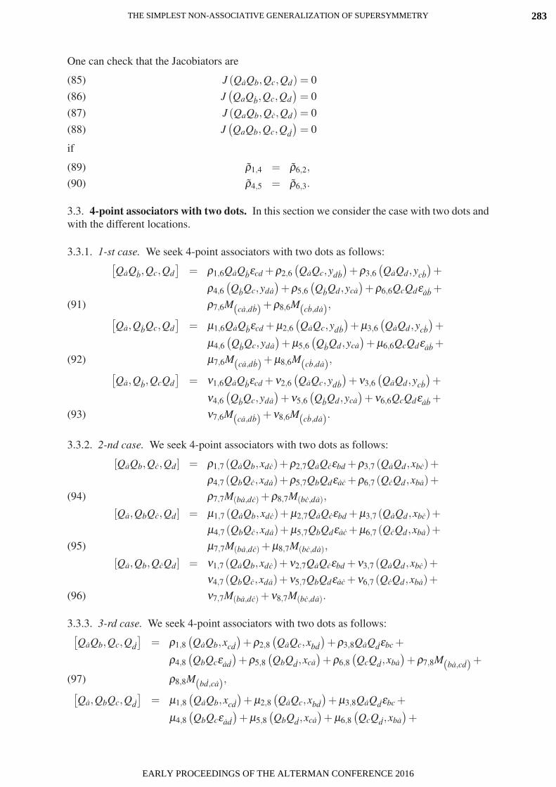
One can check that the Jacobiators are

J (QaQb,Qc,Qd) = 0(85)J(QaQb,Qc,Qd

)= 0(86)

J (QaQb,Qc,Qd) = 0(87)J(QaQb,Qc,Qd

)= 0(88)

if

ρ1,4 = ρ6,2,(89)ρ4,5 = ρ6,3.(90)

3.3. 4-point associators with two dots. In this section we consider the case with two dots andwith the different locations.

3.3.1. 1-st case. We seek 4-point associators with two dots as follows:[QaQb,Qc,Qd

]= ρ1,6QaQbεcd +ρ2,6

(QaQc,ydb

)+ρ3,6

(QaQd,ycb

)+

ρ4,6(QbQc,yda

)+ρ5,6

(QbQd,yca

)+ρ6,6QcQdεab +

ρ7,6M(ca,db) +ρ8,6M(cb,da),(91) [Qa,QbQc,Qd

]= µ1,6QaQbεcd +µ2,6

(QaQc,ydb

)+µ3,6

(QaQd,ycb

)+

µ4,6(QbQc,yda

)+µ5,6

(QbQd,yca

)+µ6,6QcQdεab +

µ7,6M(ca,db) +µ8,6M(cb,da),(92) [Qa,Qb,QcQd

]= ν1,6QaQbεcd +ν2,6

(QaQc,ydb

)+ν3,6

(QaQd,ycb

)+

ν4,6(QbQc,yda

)+ν5,6

(QbQd,yca

)+ν6,6QcQdεab +

ν7,6M(ca,db) +ν8,6M(cb,da).(93)

3.3.2. 2-nd case. We seek 4-point associators with two dots as follows:

[QaQb,Qc,Qd] = ρ1,7 (QaQb,xdc)+ρ2,7QaQcεbd +ρ3,7 (QaQd,xbc)+

ρ4,7 (QbQc,xda)+ρ5,7QbQdεac +ρ6,7 (QcQd,xba)+

ρ7,7M(ba,dc) +ρ8,7M(bc,da),(94)

[Qa,QbQc,Qd] = µ1,7 (QaQb,xdc)+µ2,7QaQcεbd +µ3,7 (QaQd,xbc)+

µ4,7 (QbQc,xda)+µ5,7QbQdεac +µ6,7 (QcQd,xba)+

µ7,7M(ba,dc) +µ8,7M(bc,da),(95)

[Qa,Qb,QcQd] = ν1,7 (QaQb,xdc)+ν2,7QaQcεbd +ν3,7 (QaQd,xbc)+

ν4,7 (QbQc,xda)+ν5,7QbQdεac +ν6,7 (QcQd,xba)+

ν7,7M(ba,dc) +ν8,7M(bc,da).(96)

3.3.3. 3-rd case. We seek 4-point associators with two dots as follows:[QaQb,Qc,Qd

]= ρ1,8

(QaQb,xcd

)+ρ2,8

(QaQc,xbd

)+ρ3,8QaQdεbc +

ρ4,8(QbQcεad

)+ρ5,8

(QbQd,xca

)+ρ6,8

(QcQd,xba

)+ρ7,8M(ba,cd) +

ρ8,8M(bd,ca),(97)[Qa,QbQc,Qd

]= µ1,8

(QaQb,xcd

)+µ2,8

(QaQc,xbd

)+µ3,8QaQdεbc +

µ4,8(QbQcεad

)+µ5,8

(QbQd,xca

)+µ6,8

(QcQd,xba

)+



µ7,8M(ba,cd) +µ8,8M(bd,ca),(98)[Qa,Qb,QcQd

]= ν1,8

(QaQb,xcd

)+ν2,8

(QaQc,xbd

)+ν3,8QaQdεbc +

ν4,8(QbQcεad

)+ν5,8

(QbQd,xca

)+ν6,8

(QcQd,xba

)+

ν7,8M(ba,cd) +ν8,8M(bd,ca).(99)

3.3.4. 4-th case. We seek 4-point associators with two dots as follows:[QaQb,Qc,Qd

]= ρ1,9

(QaQb,xdc

)+ρ2,9

(QaQc,xdb

)+ρ3,9εbcQaQd +

ρ4,9εadQbQc +ρ5,9(QbQd,xac

)+ρ6,9

(QcQd,xab

)+

ρ7,9M(ab,dc) +ρ8,9M(ac,db),(100) [Qa,QbQc,Qd

]= µ1,9

(QaQb,xdc

)+µ2,9

(QaQc,xdb

)+µ3,9εbcQaQd +

µ4,9εadQbQc +µ5,9(QbQd,xac

)+µ6,9

(QcQd,xab

)+

µ7,9M(ab,dc) +µ8,9M(ac,db),(101) [Qa,Qb,QcQd

]= ν1,9

(QaQb,xdc

)+ν2,9

(QaQc,xdb

)+ν3,9εbcQaQd +

ν4,9εadQbQc +ν5,9(QbQd,xac

)+ν6,9

(QcQd,xab

)+

ν7,9M(ab,dc) +ν8,9M(ac,db).(102)


]= ρ1,10

(QaQb,xcd

)+ρ2,10εbdQaQc +ρ3,10

(QaQd,xcb

)+

ρ4,10(QbQc,xad

)+ρ5,10εacQbQd +ρ6,10

(QcQd,xab

)+

ρ7,10M(ab,cd) +ρ8,10M(ad,cb),(103) [Qa,QbQc,Qd

]= µ1,10

(QaQb,xcd

)+µ2,10εbdQaQc +µ3,10

(QaQd,xcb

)+

µ4,10(QbQc,xad

)+µ5,10εacQbQd +µ6,10

(QcQd,xab

)+

µ7,10M(ab,cd) +µ8,10M(ad,cb),(104) [Qa,Qb,QcQd

]= ν1,10

(QaQb,xcd

)+ν2,10εbdQaQc +ν3,10

(QaQd,xcb

)+

ν4,10(QbQc,xad

)+ν5,10εacQbQd +ν6,10

(QcQd,xab

)+

ν7,10M(ab,cd) +ν8,10M(ad,cb).(105)


]= ρ1,11εcdQaQb +ρ2,11

(QaQc,xbd

)+ρ3,11

(QaQd,xbc

)+

ρ4,11(QbQc,xad

)+ρ5,11

(QbQd,xac

)+ρ6,11εabQcQd +

ρ7,11M(ac,bd) +ρ8,11M(ad,bc),(106) [Qa,QbQc,Qd

]= µ1,11εcdQaQb +µ2,11

(QaQc,xbd

)+µ3,11

(QaQd,xbc

)+

µ4,11(QbQc,xad

)+µ5,11

(QbQd,xac

)+µ6,11εabQcQd +

µ7,11M(ac,bd) +µ8,11M(ad,bc),(107) [Qa,Qb,QcQd

]= ν1,11εcdQaQb +ν2,11

(QaQc,xbd

)+ν3,11

(QaQd,xbc

)+

ν4,11(QbQc,xad

)+ν5,11

(QbQd,xac

)+ν6,11εabQcQd +

ν7,11M(ac,bd) +ν8,11M(ad,bc).(108)



3.3.7. Final form of the associators. Jacobiators. Using the relation (39) for the connectionbetween 3- and 4-point associators and the simplifications similar to those of used in section3.1, we obtain

[QaQb,Qc,Qd

]= − h

0ζ2QaQbεcd +

h0

ρ7,6M(ca,db) +h0

ρ8,6M(cb,da),(109)

[Qa,QbQc,Qd

]=

h0

µ7,6M(ca,db) +h0

µ8,6M(cb,da),(110)

[Qa,Qb,QcQd

]= − h

0ζ3QcQdεab +

h0

ν7,6M(ca,db) +h0

ν8,6M(cb,da),(111)

[QaQb,Qc,Qd] =12

h0

ρ1,7 (QaQb,xdc)+12

h0

ρ6,7 (xba,QcQd)+

h0

ρ7,7M(ba,dc) +h0

ρ8,7M(bc,da),(112)

[Qa,QbQc,Qd] =h0

µ7,7M(ba,dc) +h0

µ8,7M(bc,da),(113)

[Qa,Qb,QcQd] = −12

h0

ρ1,7 (QaQb,xdc)− 12

h0

ρ6,7 (xba,QcQd)+(114)

h0

ν7,7M(ba,dc) +h0

ν7,7M(ba,dc) +h0

ν7,7M(ba,dc) +

h0

ν8,7M(bc,da),(115)

[QaQb,Qc,Qd

]=

h0

ρ1,8(QaQb,xcd

)+

h0

ζ2QaQdεbc +h0

ρ4,8εadQbQc +

h0

ρ6,8(QcQd,xba

)+

h0

ρ7,8M(ba,cd) +h0

ρ8,8M(bd,ca),(116)

[Qa,QbQc,Qd

]= −2

h0

ρ4,8εadQbQc + µ7,8M(ba,cd) + µ8,8M(bd,ca),(117)

[Qa,Qb,QcQd

]= − h

0ρ1,8

(QaQb,xcd

)+

h0

ζ2QaQdεbc +h0

ρ4,8εadQbQc −h0

ρ6,8(QcQd,xba

)+

h0

ν7,8M(ba,cd) +h0

ν8,8M(bd,ca),(118)

[QaQb,Qc,Qd

]=

h0

ρ1,9(QaQb,xdc

)+

h0

ζ3εbcQaQd +h0

ρ4,9εadQbQc +

h0

ρ6,9(QcQd,xab

)+

h0

ρ7,9M(ab,dc) +h0

ρ8,9M(ac,db),(119)

[Qa,QbQc,Qd

]= −2

h0

ρ4,9εadQbQc +h0

µ7,9M(ab,dc) +h0

µ8,9M(ac,db),(120)

[Qa,Qb,QcQd

]= − h

0ρ1,9

(QaQb,xdc

)+

h0

ζ3εbcQaQd +h0

ρ4,9εadQbQc −h0

ρ6,9(QcQd,xab

)+

h0

ν7,9M(ab,dc) +h0

ν8,9M(ac,db),(121)

[QaQb,Qc,Qd

]=

h0

ρ1,10(QaQb,xcd

)+

h0

ρ6,10(xab,QcQd

)+

h0

ρ7,10M(ab,dc) +h0

ρ8,10M(ac,db),(122)



[Qa,QbQc,Qd

]=

h0

µ7,10M(ab,cd) +h0

µ8,10M(ad,cb),(123)

[Qa,Qb,QcQd

]= − h

0ρ1,10

(QaQb,xcd

)− h0

ρ6,10(xab,QcQd

)+

h0

ν7,10M(ab,dc) +h0

ν8,10M(ac,db),(124)

[QaQb,Qc,Qd

]= − h

0ζ3εcdQaQb +

h0

ρ7,11M(ac,bd) +h0

ρ8,11M(ad,bc),(125)

[Qa,QbQc,Qd

]=

h0

µ7,11M(ac,bd) +h0

µ8,11M(ad,bc),(126)

[Qa,Qb,QcQd

]= − h

0ζ2εabQcQd +

h0

ν7,11M(ac,bd) +h0

ν8,11M(ad,bc),(127)

where (. . . , . . .) is either commutator or anticommutator, and with the limitations

ρ7,6 − µ7,6 + ν7,6 = 0,(128)ρ8,6 − µ8,6 + ν8,6 = 0,(129)ρ7,7 − µ7,7 + ν7,7 = 0,(130)ρ8,7 − µ8,7 + ν8,7 = 0,(131)ρ7,8 − µ7,8 + ν7,8 = 0,(132)ρ8,8 − µ8,8 + ν8,8 = 0,(133)ρ7,9 − µ7,9 + ν7,9 = 0,(134)ρ8,9 − µ8,9 + ν8,9 = 0,(135)

ρ7,10 − µ7,10 + ν7,10 = 0,(136)ρ8,10 − µ8,10 + ν8,10 = 0,(137)ρ7,11 − µ7,11 + ν7,11 = 0,(138)ρ8,11 − µ8,11 + ν8,11 = 0.(139)

One can check that the Jacobiators are (here we consider the simplest case xa,b = M(ab,cd) = 0)

J(QaQb,Qc,Qd

)= 0,(140)

J(Qa,QbQc,Qd

)= − h

0ζ2εcd

[Qa,Qb

]− h0

ζ3εab [Qc,Qd] ,(141)

J(Qa,Qb,QcQd

)= 0,(142)

J (QaQb,Qc,Qd) = − h0

ζ2εbd [Qa,Qc]− h0

ζ3εac [Qb,Qd] ,(143)

J (Qa,QbQc,Qd) =h0

ζ2εbd [Qa,Qc]+h0


J (Qa,Qb,QcQd) = − h0

ζ2εbd [Qa,Qc]− h0


J(QaQb,QcQd

)=

h0

ζ2εbc[Qa,Qd

]+

h0

ζ3εad [Qb,Qc] ,(146)

J(Qa,QbQc,Qd

)= 0,(147)

J(Qa,Qb,QcQd

)=

h0

ζ2εbc[Qa,Qd

]+

h0

ζ3εad [Qb,Qc] ,(148)

J(QaQb,Qc,Qd

)=

h0

ζ2εad[Qb,Qc

]+

h0

ζ3εbc [Qa,Qd] ,(149)



J(Qa,QbQc,Qd

)= 0,(150)

J(Qa,Qb,QcQd

)=

h0

ζ2εad[Qb,Qc

]+

h0

ζ3εbc [Qa,Qd] ,(151)

J(QaQb,Qc,Qd

)= − h

0ζ2εac

[Qb,Qd

]− h0

ζ3εbd [Qa,Qc] ,(152)

J(Qa,QbQc,Qd

)=

h0

ζ2εac[Qb,Qd

]+

h0


J(Qa,Qb,QcQd

)= − h

0ζ2εac

[Qb,Qd

]− h0


J(QaQb,QcQd

)= 0,(155)

J(Qa,QbQc,Qd

)= − h

0ζ2εab

[Qc,Qd

]− h0

ζ3εcd [Qa,Qb] ,(156)

J(Qa,Qb,QcQd

)= 0,(157)

(158)

if

ρ4,8 = ζ3,(159)ρ4,9 = ζ2,(160)

Qa,Qb

= Qa,Qb= 0.(161)

3.4. 4-point associators with two dots. This case is identical to subsection 3.2 after replacinga ↔ a.

4. THE CONNECTION WITH SUPERSYMMETRY

Now we want to pounce on supersymmetry. In this case the operators Qa,b obey thefollowing anticommutators

Qa,Qb =

Qa,Qb= 0,(162)

Qa,Qa = QaQa +QaQa = 2σ µaaPµ ,(163)

where the operator P can be a nonassociative generalization of standard accosiative operator−ih∂µ ; the Pauli matrices σ µ

aa,σaaµ are defined in the standard way

σ µaa =

(1 00 1

),

(0 11 0

),

(0 −ii 0

),

(1 00 −1

)(164)

σaaµ =

(1 00 1

),

(0 11 0

),

(0 i−i 0

),

(1 00 −1

)(165)

with the orthogonality relations for the Pauli matrices

(166) σaaµ σν

aa = 2δ νµ , σaa

µ σ µbb

= 2δ ab δ a

b .

Let us note the following interesting relation which follows from (30)

(167) (QaQb)Qb =− h0

ζ1Qbεab.

Roughly speaking, one can say that this expression “destroys” sometimes Q2a = 0 property of

Grassmann numbers. This results in distinctions between supersymmetries based on associativeand nonassociative generators. But this difference will be (in the dimensionless form) of theorder of lPl/0, where 0 is some characteristic length. For example, if 0 = Λ−1/2 (where Λ isthe cosmological constant) then this difference will be ≈ 10−120.



5. SUPERSYMMETRY, HIDDEN VARIABLES, AND NONASSOCIATIVITY

In this section we want to consider a possible connection between supersymmetry, hiddenvariables, and nonassociativity.

First of all we want to remind what is the hidden variables theory. In Wiki [11] onecan find the following definition of hidden variables theories ”. . . hidden variable theories wereespoused by some physicists who argued that the state of a physical system, as formulatedby quantum mechanics, does not give a complete description for the system; i.e., that quan-tum mechanics is ultimately incomplete, and that a complete theory would provide descriptivecategories to account for all observable behavior and thus avoid any indeterminism. . . .

. . . In 1964, John Bell showed that if local hidden variables exist, certain experimentscould be performed involving quantum entanglement where the result would satisfy a Bellinequality. . . .

Physicists such as Alain Aspect [12] and Paul Kwiat [13] have performed experimentsthat have found violations of these inequalities up to 242 standard deviations[14] (excellentscientific certainty). This rules out local hidden variable theories.

. . . Gerard ’t Hooft [14, 15] has disputed the validity of Bell’s theorem on the basis of thesuperdeterminism loophole and proposed some ideas to construct local deterministic models.“

We want to pay attention to what we talked about the associative observables. Thatis natural for physical quantities in quantum mechanics. But in Ref. [16] the possibility ofconsideration of nonassociative hidden variables is discussed. In this case these quantities areunobservable ones.

Let us consider what happens in our case. We have supersymmetric decomposition of(probably generalized) momentum operator (163). The constituents Qa,a are unobservable ac-cording to the nonassociative properties (30)-(37) and (55)-(57). Following this way, we cansay that we have unobservable nonassociative operators Qa,a that are similar to hidden vari-ables. The main difference compared with the standard hidden variables is unobservability ofthe nonassociative hidden-like variables.

6. DISCUSSION AND CONCLUSIONS

Thus we have considered a nonassociative generalization of supersymmetry. We haveshown that: (a) one can choose such a form of 3-point associators that the corresponding Ja-cobiators are zero; (b) there is the relation between 3- and 4-point associators; (c) using theseexpressions, one can find 4-point associators.

We have seen that in all definitions of associators there is the Planck constant and somecharacteristic length 0. The presence of the Planck constant permits us to make natural as-sumptions that these associators can be regarded as a nonassociative generalization of theHeisenberg uncertainty principle. In this case the characteristic length 0 will be a new fun-damental constant, and the corrections arising in this case have the order of h/0. For exam-ple, if 0 ≈ Λ−1/2 (where Λ is the cosmological constant) then the dimensionless corrections≈ 10−120, i.e., are negligible. Instead of introducing a fundamental length 0, we can introducea fundamental momentum P0 = h/0. Physical consequences of introducing new fundamentalquantities 0 or P0 (that are consequences of nonassociativity) are:

• There appears a minimum momentum P0.• There appears a maximum length 0.



• The appearance of the maximum length 0 leads to the fact that the curvature is boundedbelow: Rmin ≈ 1/2

0.• The minimum momentum P0 and the maximum length 0 are connected by the Heisen-

berg uncertainty principle: P00 ≈ h.• The experimental manifestation of possible nonaccosiativity can arise only for a physi-

cal phenomenon when either the momentum ≈ P0 ≈ 10−60kg ·m · s−1 or on the scalesl ≈ 0 ≈ Λ−1/2 ≈ 1026m (if the fundamental length 0 ≈ Λ−1/2).

We have also discussed a possible interpretation of nonassociative supersymmetric generatorsQa,a as hidden-like variables in quantum theory. The main idea here is that the nonassociativityleads to unobservability of these variables.

REFERENCES

[1] M. Gunaydin and F. Gursey. Quark statistics and octonions. Phys. Rev., D9 (1974) 3387-3391.[2] M. Gogberashvili. Octonionic electrodynamics, J. Phys. A 39 (2006) 7099-7104; [arXiv:hep-th/0512258].[3] M. Gogberashvili. Octonionic version of Dirac equations, Int. J. Mod. Phys. A 21 (2006) 3513-3524,

[arXiv:hep-th/0505101].[4] M. Gunaydin and D. Minic, Fortsch. Phys. 61, 873 (2013) [arXiv:1304.0410 [hep-th]].[5] M. Bojowald, S. Brahma and U. Buyukcam, Phys. Rev. Lett. 115 (2015) 22, 220402;

doi:10.1103/PhysRevLett.115.220402, [arXiv:1510.07559 [quant-ph]].[6] V. Dzhunushaliev, Found. Phys. Lett. 19, 157 (2006); doi:10.1007/s10702-006-0373-2, [hep-th/0502216].[7] S. Okubo, “Introduction to octonion and other nonassociative algebras in physics,” Cambridge University

Press, 1995.[8] F. Gursey and C-H Tze, “On the Role of Division, Jordan, and Related Algebras in Particle Physics,” World

Scientific, 1996.[9] V. Dzhunushaliev, “Three-point non – associative supersymmetry generalization and weak version of non –

commutative coordinates,” arXiv:1504.00573 [hep-th].[10] V. Dzhunushaliev, “Nonassociative Generalization of Supersymmetry,” Adv. Appl. Clifford Algebras, 2015

Springer Basel, DOI 10.1007/s00006-015-0580-7; arXiv:1302.0346 [math-ph].[11] https://en.wikipedia.org/wiki/Hidden_variable_theory.[12] A. Aspect, P. Grangier and G. Roger, Phys. Rev. Lett. 49, 91 (1982).[13] P. G. Kwiat, E. Waks, A. G. White, I. Appelbaum and P. H. Eberhard, Phys. Rev. A 60, 773 (1999) [quant-

ph/9810003].[14] Gerard ’t Hooft, “The Free-Will Postulate in Quantum Mechanics”, arXiv:quant-ph/0701097.[15] Gerard ’t Hooft, “Entangled quantum states in a local deterministic theory”, arXiv:0908.3408 [quant-ph].[16] V. Dzhunushaliev, “Non – associativity, supersymmetry and hidden variables,” J. Math. Phys. 49, 042108

(2008); DOI:10.1063/1.2907868; arXiv:0712.1647 [quant-ph].



GA AND GC APPLIED TO PRE-SPATIAL ARITHMETIC SCHEMETO ENHANCE MODELLING EFFECTIVENESS

IN BIOPHYSICAL APPLICATIONS

R.A. Fiorini a

a Departament of Electronics, Information and BioengineeringPolitecnico di Milano University


ABSTRACT. The classic vector analysis is unable to describe the Quantum Mechanics, Rela-tivity and Quantum Field Theory so that an increasing attention to the geometric algebra (GA)and geometric calculus (GC) has been paid. In arbitrary multiscale complex system modellingthe bottom-up discrete approach under the ”discreteness hypothesis” is mandatory to achieveeffective operative solutions. We present an exponential, pre-spatial arithmetic scheme (”all-powerful scheme”) to overcome the limitation of the traditional top-down probabilistic mod-elling veil opacity. CICT (computational information conservation theory) new awareness ofa discrete hyperbolic geometry subspace (reciprocal-space, RS) of coded heterogeneous hyper-bolic structures, underlying the familiar Q Euclidean direct-space (DS) surface representation,shows that any natural number n in N has associated a specific, non-arbitrary exterior phaserelationship that we have to take into account to full conserve overall system component infor-mation content by computation in DS. GA and GC unified mathematical language with CICTcan offer a competitive and effective ”Science 2.0” universal arbitrary multiscale computationalframework for biophysical and advanced applications.

1. INTRODUCTION

In his classical book on quantum mechanical principles [1], Heisenberg delineates withhis usual clarity two possible ways to build quantum mechanics (QM), both of which werecoherent with the uncertainty principle:

• (a)- a space-time description tending to save the classical concepts by means of a sta-tistical connection;

• (b)- adopting a pre-spatial mathematical scheme and a different concept of causality.

Quantum events only happen in interactions between systems, and the fact that a quantum eventhas happened is only true with respect to the systems involved in the interaction. The uniqueaccount of the state of the world of the classical theory is thus fractured into a multiplicityof accounts, one for each possible ”observing” physical system. In ordinary QM we assumethat the entropy is a vector that represents superposition state of the pure states. Any observerby a measure can see only one of the possible values of the superpose vector of entropies.Therefore, we can consider the entropy of a quantum system as a vector of the superpositionof many different entropies whose values are conditioned by the observer. Any observer makesthe system in superposition collapse to a classical value of entropy, i.e. it fixes classical in-formation by a measurement. When the observer does not interact with a quantum system,the composed system given by the quantum ”microsystem+observer” (and thus, somewhat theuniverse) is in an entangled state. When the observer interacts with the ”microsystem” underconsideration thus becoming an active element, the composed system given by the ”quantummicrosystem+observer” is in a pure state and follows the classical thermodynamics defined byone specific entropy and, in correspondence, the measured variable of the system under con-sideration takes the measured value. The superpose vector of the quantum entropies (whose

290


values are conditioned by the observer) is the fundamental entity that explains in what sense,when a quantum event happens, it happens only with respect a peculiar observing physical sys-tem. In quantum mechanics, one can say that a variable of a quantum system takes the valueq because the vector given by a superposition of different Boltzmann entropies collapses toone specific entropy which corresponds to the value q of the variable under consideration: aninteraction between the quantum system and an observer happens which produces the collapseof the vector of the superposed entropies into one specific entropy and the observer involvedin this interaction measures just the value q of the variable under consideration. As concerningpoint (a), according to personal experience, geometric algebra (GA), geometric calculus (GC)and spacetime algebra (STA) [2, 3] are the current best tools to satisfy those requirements byreliable computational point of view. In the 1930s there was no cogent reason to choose thesecond way (b). Nowadays, we know that incredibly small groups of atoms, much too small todisplay exact statistical laws, do play a dominating role in the very orderly and lawful eventswithin a living organism, so approach (a) cannot be followed. They have control of the ob-servable large-scale characteristics of its functioning; and in all this very sharp and very strictbiological laws are displayed. The great revelation of quantum theory, discovered by MaxPlanck in 1900, is that features of a discreteness were discovered in the Book of Nature at sys-tem microscale (nanoscale) level, in context in which anything other than continuity seemedto be absurd according to the views held until then at macroscale level. Quantum nonlocalityoffers a valid reason to explore a different approach where the nonlocal features of QM are notnecessarily restricted to the entangled amplitudes, but are instead connected to a time-reversalapproach, or some timeless background [4]. In fact, according to the principle of complemen-tarity, there is also another representation of the uncertainty relation where the phase assumes aprecise value; this representation which focuses on the wave-like features of the system cannotbe assumed simultaneously with the particle representation [5, 6]. The relation between thesetwo representations is expressed by the uncertainty relation, similar to the Heisenberg relationbetween position and momentum:

(1) ∆N∆Φ ≥ 1/2

connecting the uncertainty of the number of quanta (particle structure of the system) ∆N andthe uncertainty of the phase (which describes the rhythm of fluctuation of the system) ∆Φ. Forpoint (a) approach, the difference between classical and quantum information is similar to thedifference between Euclidean and non-Euclidean geometry in the parameter space determinedby the quantum entropy. Traditionally, superposition states characteristic of quantum mechan-ics are determined by the deformation of the geometry of the background and are associatedwith a vector of superposed entropies. Here, we like to present a new approach where we sug-gest a non-Euclidean geometry emerging out of optimally combined phased generators as thesource of a quantum information. As a sound example, in this paper, first we focus our attentionon the relativistic electrodynamics inertial observer (IO) space-time split (STS) case, supportedby spacetime algebra (STA) as spacetime representation system, to show how the full vectorinformation content of rational correspondence at higher representation level (macroscale) forIO STS cannot be conserved by traditional approach (point (a)). Then, we present and discussCICT (Computational Information Conservation Theory) solution by a pre-spatial arithmeticscheme to overcome and minimize the probabilistic modeling veil opacity (point (b)). We liketo show how STS invariant physical quantities can be related to the variables employed by aspecific interacting inertial observer (IO), with large information dissipation unavoidably, ifspecific computational awareness and care are not taken into account. To gain a better under-standing about the operational compromise offered by the inertial observer spacetime splittingand the Space-Time Algebra (STA) main properties, Subsection 1.1 and Subsection 1.2 arepropedeutic to later sections.

G.A. AND G.C. APPLIED TO PRE-SPATIAL ARITHMETIC SCHEME TO ENHANCE MODELING EFFECTIVENESS 291


1.1. Inertial Observer (IO) Spacetime Splitting. Here we follow the line of thought reportedin Hestenes’ STA [3, 7], emphasizing the fundamental role of the IO. STA is built up from com-binations of one time-like basis vector γ0 and three orthogonal space-like vectors γ1,γ2,γ3,under the multiplication rule [3]:

(2) γµγν + γνγµ = 2ηµν ,

where ηµν is the Minkowski metric with signature (+ - - -). We choose the signature here thatwill produce the STA that correctly contains the relative Euclidean 3-space (direct space, DS)as a proper subalgebra. Since there are one positive sign and three negative signs in this dotproduct, we say that it has a mixed signature (+ - - -) and denote the vector space of 4-vectors asM1,3 to make this signature explicit. So, all physical vector quantities in special relativity arepostulated to be 4-vectors in M1,3 that satisfy the Minkowski metric. These vectors are geomet-ric quantities that do not depend on the choice of reference frame, so they shall be called properrelativistic objects in what follows. Importantly, the Minkowski metric is qualitatively differentfrom the standard Euclidean dot product since it does not produce a positive length. Indeed,the mixture of positive and negative signs can make the length of a vector positive, negative, orzero, which produces three qualitatively different classes of vectors. We call these classes ofvectors timelike, spacelike, and lightlike, respectively. Physically speaking, STA is a completeand natural algebraic language for compactly describing physical quantities that satisfy the pos-tulates of special relativity. Mathematically speaking, it is the largest associative algebra thatcan be constructed with the vector space of spacetime equipped with the Minkowski metric.It is an orthogonal Clifford algebra (CA) [8], which is a powerful tool that enables manifestlyframe-independent and coordinate free manipulations of geometrically significant objects. BySTA, Maxwell’s equations reduce to a terse single equation:

(3) ∇F = µ0cJ,

where c is the speed of light, µ0 is the parameter that international Standards Organizations callthe ”magnetic constant,” commonly called ”vacuum permeability,” with the ”defined” value µ0= 4π · 10−7H ·m−1 [9], with usual definition of variables [3]. The classical approach startstaking into consideration a generic electromagnetic field F , described by Riemann–Silbersteinvector [10]. The field F is defined as a complexified 3-dimensional vector field [11]. The valueof F at an event is a bivector according to GA [2]. The field bivector F is the same for allobservers; there is no question about how it transforms under a change of reference system.However, it is easily related to a representation of coupled electric and magnetic fields in agiven inertial system (inertial observator, IO). GA can show how spacetime invariant physicalquantities can be related to the variables employed by IO quite easily. An inertial system isdetermined by a single unit time-like vector γ0, which can be regarded as tangent (with exactapplication point P unknown) to the worldline of an observer at rest in the system. Accordingto STA this vector determines a ”split” of ST into Space and Time, in other words a projectionfrom 4-dimensional space into (3+1)-dimensional space, with a chosen reference frame bymeans of the following two operations [3]:

• a collapse of the chosen time axis, yielding a 3D space spanned by bivectors;• a projection of the 4D space onto the chosen time axis, yielding a 1D space of scalars;

which are most simply expressed by the equation:

(4) xγ0 = t +x,where t = x · γ0 and x = x∧ γ0. This is just an example of a projective transformation in CA.It is a linear mapping of each spacetime point x(γ1,γ2,γ3) into a scalar t designating a timeand a vector x designating a position. The position vectors for all spacetime points compose a3-dimensional Euclidean vector space R3. We denote the vectors in R3 with boldface type to

G.A. AND G.C. APPLIED TO PRE-SPATIAL ARITHMETIC SCHEME TO ENHANCE MODELING EFFECTIVENESS292


distinguish them from vectors in R1,3. Let Rp,q denote a vector space of dimension n = p+ qover the reals consisting of a p-dimensional subspace of vectors with positive signature orthog-onal to a q-dimensional subspace of vectors with negative signature [3]. We argue that it isexactly at this point that ”both/and” becomes ”either/or” representation by usual Science 1.0approach. In other words, quantum system representation is mapped to classical system addi-tive representation with loss of overall system fundamental coherence information (the field Finformation phase connecting time component to space component coherently into their prim-itive spacetime continuum, at their original gauge level). Classically, the position vectors forall spacetime points compose a 3-dimensional Euclidean vector space R3. In this context, ”or-thogonality” of vectors means a vanishing inner product. Let Rp,q denote the CA generated bythe vectors of Rp,q and let Rk

p,q be the(n

k

)-dimensional subspace of k-vectors in Rp,q. Elements

of the Rkp,q 1-dimensional subspace are called ”pseudoscalars” [2] of Rp,q or Rp,q. An arbitrary

element of Rp,q is called a ”multivector” or Clifford number [2]. The primary reference-frame-independent objects of special relativity (i.e., scalars, 4-vectors, bivectors/anti-symmetric rank-2 tensors, pseudo-4-vectors, and pseudoscalars) are unified as distinct grades of a single objectknown as a ”multivector.” An element of grade k geometrically corresponds to an orientedsurface of dimension k (e.g., 4-vectors are line segments, while bivectors are oriented planesegments) [2]. For the important case of a vector space with Euclidean (positive) signature, itis convenient to introduce the abbreviations Rn ≡ Rn,0, Rn ≡ Rn,0 and Rk

n ≡ Rkn,0. The equation

x = x∧ γ0 tells us that a vector in R3 is actually a bivector in R21,3. In fact, R3 consists of the set

of all bivectors in R21,3 which have the vector γ0 as a factor. Algebraically, this can be charac-

terized as the set of all bivectors in R21,3 which anticommute with γ0. This determines a unique

mapping of the electromagnetic bivector F into the GA R3 of the given inertial system. In fact,the space-time split of F by γ0 is obtained by decomposing F into a part:

(5) E = 1/2(F − γ0Fγ0),

which anticommutes with γ0 and a part:

(6) BcI = 1/2(F + γ0Fγ0),

which commutes with γ0, so we have:

(7) F = (E + BcI),

where I = γ0γ1γ2γ3 = γ0123 is the unit pseudoscalar. Some authors prefer to multiply the righthand side by an overall constant where

√ε0 is the permittivity of free space (vacuum):

(8) F = (E + Bci)√

ε0

or equivalently, by an algebraic point of view for representation systems [12], and more pre-cisely, by a computational point of view for description systems [13]:

(9) F = (E + Bci)/√

µ0.

F is defined as a complexified 3-dimensional vector field. The value of F at an event is a bivec-tor (a ”bivector” is the vector part of a biquaternion; the biquaternions are just the complexifi-cation of the (real) quaternions). Incidentally, by QM point of view, the quantum mechanicalderivation that produces eq.9 also produces Maxwell’s vacuum equations in an intriguing formthat resembles the Dirac equation for massless spin-1 particles [14, 15, 16, 17, 18, 19, 20].Treating the complex vector in eq.9 as a single-particle wave function in the first-quantizedquantum mechanical sense produces consistent results, and suggests that this vector should bea more natural representation for classical e.m. fields as well. Remarkably, performing the stan-dard second-quantization procedure using the complex Riemann—Silberstein wave function ineq.9 identically reproduces the correctly quantized e.m. field [16, 17, 18] in QFT (Quantum



Field Theory). Although BI commutes with γ0, B must anticommute since I does. Therefore,we are right to denote B as a vector in R3. By iteratively appending all objects generated bythe wedge product to the initial vector space M1,3, we construct the full Clifford STA C l1,3.This notation indicates that the STA is a CA generated from the metric signature (+ - - -). Im-portantly, all components in this CA are purely real. In this case, the GA generated by R3 isidentical with the even subalgebra of R1,3, so we write:

(10) R3 = R+1,3.

Moreover, eq.4 determines a split of the bivectors in R21,3 into vectors and bivectors of R3, as

expressed by writing:

(11) R21,3 = R1

3 +R23.

This split is not unique, however, as it depends on the choice of the vector γ0. A completediscussion of space-time splits is given in [2, 3]. Finally, we should point out that the purposeof STS is merely to relate invariant physical quantities to the system macroscale variablesemployed by specific IO.

1.2. STA Fundamental Properties. STA is the Hestenes’ name for the CA C l1,3(R), orequivalently the geometric algebra G4 ≡ G(M1,3). Of course, E and B in eq.7 are just theelectric and magnetic fields in the γ0-system, and the split of F into electric and magnetic fieldswill be different for different inertial systems (different IOs). We argue that it is exactly at thispoint that quantum system representation is mapped to classical system additive representa-tion with loss of overall system fundamental coherence information (the field F informationphase connecting time component to space components coherently into their primitive space-time continuum, at their original gauge level) by traditional Physics approach. As we brieflyindicated, the embedding of CAs C l3,0 ⊂ C l1,3 motivated our choice of metric signature forspacetime to be (+ - - -). The new basis vectors share the algebra of the gamma matrices but areusually not equated with them. This embedding is part of a larger sequence of CA embeddingsstarting from C l0,0 ⊂ C l0,1 ⊂ C l0,2 ⊂ C l3,0 ⊂ C l1,3 ⊂ C l4,1 ⊂ C l2,4 which corresponds to,respectively, the real numbers, complex numbers (Schrodinger spinors), quaternions (Hamil-ton spinors), relative 3-space (Pauli spinors), spacetime/electromagnetism (Maxwell spinors),relativistic electron (Dirac spinors), and conformal space (Penrose twistors) [21]. Here, welike to focus our attention to the fact that the classic vector space M1,3 does not contain thecomplete physical picture implied by special relativity, since it must be augmented by quanti-ties like Fµν to obtain the complete picture of special relativity in a systematic and principledway. Indeed, standard treatments of electromagnetism, involving relative 3-vectors, use boththe symmetric dot product and the antisymmetric vector cross product to properly discuss thephysical implications of the theory. The classic vector space M1,3 only specifies the relativis-tic version of the dot product in the form of the Minkowski metric. As you can see, withoutintroducing the proper relativistic notion of the wedge product (proper generalization of thevector cross product to relativistic 4-vectors) the physical picture of spacetime is incomplete.Mathematically, the introduction by STA of a product on a vector space creates an algebraand the wedge product is precisely Grassmann’s exterior wedge product, adopted by Cartanto define differential forms [22]. The wedge product enlarges the mathematical space in or-der to properly accommodate quantities like the electromagnetic field tensor Fµν . Evidently,the intrinsic complex structure inherent to the geometry of spacetime has deep and perhapsunder-appreciated consequences for even our classical field theories. The complex vector fromeq.7 will appear naturally as a relative 3-space expansion of a bivector field, which is a propergeometric (and thus frame-independent) object in spacetime. Moreover, this bivector fieldwill have a crucial fundamental difference from Riemann–Silberstein vector [12]: the scalarimaginary i in Riemann–Silberstein vector will be replaced by an algebraic unit pseudoscalar



I (also satisfying I2 = −1) that is intrinsically meaningful to and required by the geometricstructure of spacetime. This replacement makes the complex form of F reference-frame inde-pendent, which is impossible when the mathematical representation is restricted to the usualscalar imaginary i only. The electromagnetic field is an irreducibly complex object with anintrinsic phase. This phase necessarily involves the intrinsic pseudoscalar (unit 4-volume) I ofspacetime, and it is intimately related to the appearance of electromagnetic waves and circularpolarizations, with no need for any ad-hoc addition of a complex scalar field. As a matter offact, this replacement of the scalar i with I has to be systematic throughout the electromagnetictheory, where it appears in electromagnetic waves, elliptical polarization, the normal variablesfor canonical field mode quantization, and the dual symmetric internal rotations of the vacuumfield, to arrive to full ST system macroscale representation information conservation. From amultiscale complex system computational perspective (see [23] for a definition of multiscalecomplex system), all approaches that use a top-down scale-free approach allow for startingfrom an exact global solution panorama of analytic solution families, which offers a shallowlocal solution computational precision to real specific needs (in other words, from global tolocal point of view overall system information is not conserved, as misplaced precision leadsto information dissipation). In fact, usually further analysis and validation (by probabilisticand stochastic methods) is necessary to get localized computational solution of any practicalvalue, in real application. A local discrete solution is worked out and computationally approx-imated as the last step in their line of reasoning, that started from an overall continuous systemapproach (from continuum to discreteness hypothesis approach). In arbitrary multiscale com-plex system modelling the bottom-up discrete approach under the ”discreteness hypothesis” ismandatory to achieve effective solutions [23]. To design and develop more robust, resilient andantifragile cyber-physical multiscale complex system modelling, we need novel tools to com-bine effectively and efficiently analytical asymptotic exact global solution panoramas to deeplocal computational precision achievement, to overcome the limitation of the traditional top-down probabilistic modelling veil opacity. We can achieve that goal taking into considerationthe CICT computational system pre-spatial arithmetic scheme.

2. CICT PRE-SPATIAL ARITHMETIC SCHEME

It is possible to show a new point of view for computational space representation, wherethe complex upper half-plane can naturally emerge by the interplay of the coupled inversionof two counter oriented upper quarter planes. That representation can be even read as the self-reflexion of a reciprocal conformal relation of an ”Outer Symbolic Representation” (OSR) toits corresponding reflected fundamental ”Inner OpeRational Representation” (IOR) and vice-versa, where D in Z, A = 1/D and D = 1/A, and DA = AD = 01.0 , for positive oriented upperquarter-space (right upper quarter plane) and DA = AD = −01.0 , for negative oriented upperquarter-space (left upper quarter plane). The relationship of these two counter-oriented up-per quarter-spaces can be thought as a reciprocally projective conformal correspondence to bethe first operative example in literature for explicit self-reflexive oriented numeric representa-tion space [24], that can be used as powerful reference framework to develop ”OpeRational”Representation (OR)[25] applications for maximum information conservation (i.e. minimuminformation dissipation). For the sake of simplicity, we show main properties of one orientedupper quarter-space only, because the second one is just its reflection with respect a verticalaxis, so LTR (Left-To-Right) representation can turn into RTL (Right-To-Left) representationand vice-versa. In virtue of this relationship, a direct representation turns into additive com-plemented representation and vice-versa, when needed. The same information content can gettwo different numerical representations which can resonate to each other freely, at the sametime, with respect to an inversive reference boundary element (i.e., centered unitary segment



in 1-d, unitary circumference in 2-d, unitary sphere in 3-d, unitary ipersphere in 4-d, etc.) be-tween an nth-dimensional OSR (Outer Space Representation) and a correspondent IOR (InnerSpace Representation), according to the Kelvin transform [26]: an nth-dimensional OSR to itscorresponding IOR and vice-versa. Reversing a convergent sequence into a divergent one andvice-versa is the fundamental property to reach information conservation, i.e. information re-versibility. Traditional Number Theory and modern Numeric Analysis use mono-directionalinterpretation (LTR) for Q Arithmetic single numeric group generator, so information entropygeneration cannot be avoided in contemporary computational algorithm and application. Onthe contrary, according to CICT , it is quite simple to show information conservation and gen-erator reversibility, by using basic considerations only. We like to show our new point of viewfor number interpretation and processing discussing two fundamental topics in order to achievemore convenient and effective numeric algorithm development: Arithmetic Closure and Infor-mation Conservation in Section 2.1., and Exponential Periodic Closure and OECS (OptimizedExponential Cyclic Sequence) in Section 2.2.

2.1. Arithmetic Closure and Information Conservation. Let us consider fraction 1/D, whereD in Z, or Egyptian fraction, with no loss of generality for common fraction. Common frac-tion, given by Egyptian fraction multiplied by a ∈ Z, is considered a simple integer divisionusually. The first repetition of basic period for reptend corresponds to the first full scale intervalwhere number information can be conserved: we call it ”Representation Fundamental Domain”(RFD) [25]. In general, D, the denominator of the considered OSR, is given by a finite decimalword of length W digits. From IOR X , the related RFDL can be obtained, by a numeric wordlength of LX digits. Elementary number theory considerations give us worst case word lengthLX , with no loss of information, by:

(12) LX = D−1

digits, if and only if 10 is a primitive root modulo D. Otherwise LX is a factor of D− 1. Ifthe period of the corresponding repeating decimal to 1/D for prime D is equal D−1, then therepeating decimal part is called ”cyclic number” and D can be referred as ”primitive number”or ”solid number” (SN) of order 1 by CICT or ”full reptend prime” elsewhere [27]. Thus aSN is necessarily prime. It is a sufficient qualification. Conversely a prime number may notbe a SN of order 1. So, the usual worst case word length LX for X , given by eq.12, can getRFDL with no loss of information, related to D, just in case D is SN of order 1 or SN1 forshort. In this way, an OSR 1/D can be associated to a corresponding IOR and vice-versa, andan IOR RFDL to a corresponding OSR and vice-versa, which are able to resonate freely toeach other (we can say we got ”resonant representation correspondence”). In classic arithmeticlong division algorithm (the one you learn to divide at elementary school), usual dominantresult (quotient, Q) is important, and traditionally minority components (remainders, R) arealways discarded. So, with no loss of generality, let us consider, the first integer to show SN1property manifestly, that is number ”7.” In this case D = 07.0, so that worst case length analysisgives LX = D− 1 = 6 digits. Recording of quotient Q and remainder R evolutive informationgeneration is needed. The full-information content of long division 1/7 would be stored intotwo decimal coupled words < Q,R > of length MQR = (6+6) digits in total, for exact arbitrary



precision computation. In fact, for long division 1 by 7, we have:

L1 = 1, Q1 = 1/101, R1 = 3/101

L2 = 2, Q2 = 14/102, R2 = 02/102

L3 = 3, Q3 = 142/103, R3 = 006/103

L4 = 4, Q4 = 1428/104, R4 = 0004/104(13)

L5 = 5, Q5 = 14285/105, R5 = 00005/105

L6 = 6, Q6 = 142857/106, R6 = 000001/106

L7 = 7, Q7 = 1428571/107, R7 = 0000003/107

and LX = 6, and Tp = 6. Therefore, 7 is just a SN1 and its full information content is capturedby a six-digit word length RFD6, for Q6 and the same for R6. Eqs. 13 sum up the first stages ofelementary long division of 1 by 7. But from eqs. 13 it is straightforward to note too:

(14)17=

110

∞

∑k=0

(3

10

)k

=14102

∞

∑k=0

(02102

)k

=142103

∞

∑k=0

(006103

)k

= . . .

The Remainder RL, at any computation evolutive stage, is the fixed multiplicative ratio of aformal power series associated to optimal decimal representations of 1/7, at increasing arbitraryaccuracy levels. Thus 1/7 associated information content can be lossless compressed down tominimal MQR = (1+ 1) digits in total. As a matter of fact, any word couple < QL,RL > canbe thought to be equivalent to and can represent a different real measurement instrument class,defined by RFD word length LX . It is easy to see that, in general, but not always, the greaterD, the lengthier LX , and greater the achievable compression ratio Ew. In this simple caseEw = (2 ∗ 6)/2 = 6 : 1, for number 7. Furthermore, by realizing that the remainder R1 is thefixed multiplicative ratio of a power series, the computation of 3n (mod 7) for n = 1,2,3, . . .,till its exponential closure, gives the ”Fundamental Cyclic Remainder Sequence” (FCRS):

(15) R1 = 3, R2 = 2, R3 = 6, R4 = 4, R5 = 5, R6 = 1

from which the ”Fundamental Cyclic Quotient Sequence” (FCQS) can be readily regeneratedby 7∗Rn (mod 10):

(16) Q1 = 1, Q2 = 4, Q3 = 2, Q4 = 8, Q5 = 5, Q6 = 7.

So, quotient and remainder information can always be regenerated anew by remainder infor-mation only, but not vice-versa. In fact, starting from Q1 = 1,R1 = 3, we get: Q2 = Q1/10+Q1R1/100 = 13/100 and raw r2 = 09/100. Now r2(mod07) gives q2 = 1 and R2 = 02/00. Wecan use this information to obtain the final exact value of Q2 and R2 at A = 10−2 accuracy level,in the following way:

(17) Q2 = Q1/10+Q1R1/100+q2/100 = 14/100 and R2 = 02/100

Again, starting from Q2 = 14/100, R2 = 02/100, we get:

(18) Q4 = 14/100+Q2R2/10000 = 1428/10000 and R4 = 0004/10000,

and so on. In this way, with remainder knowledge only, it is always possible to regenerateexact quotient and new remainder information at any arbitrary accuracy, with full informationconservation. It is like to process tail information to regenerate the associated body information.Thanks to the above properties, the division algorithm can become free from trial and error likein Finite Segment P-adic representation systems, but with no usually associated coding burden[28]. For every OSR D≥D, where D is the additive 10W complement of D, i.e. D= (10W −D),



the fundamental related IOR, for LTR sequences, it is immediately given, for all values of D inZ, by the following formal power series:

(19)1D

=∞

∑k=0

110W

(D

10W

)k

,

where W is the word representation precision length of the denominator D. When D > D theformal power series of eq.19 can be rescaled modD, to give multiple convergence paths to1/7, but with different ”convergence speeds.” The total number of allowed convergent paths,as monotonic power series, is given by the corresponding QL value, at the considered accuracylevel. For instance, in the case of:

(20)1

07=

∞

∑k=0

1102

(93102

)k

,

we see that D = 07, W = 2, A = 10−2 and D = 93 > D = 07. Therefore, re-scaling the fixedmultiplicative ratio modD, we have:

107

=∞

∑k=0

2102

(86102

)k

,(21)

107

=∞

∑k=0

3102

(79102

)k

,(22)

...107

=∞

∑k=0

14102

(02102

)k

,(23)

for a total of 14 conservative paths converging to the same limit value 1/07, with different con-vergence velocities till a maximum value (Q2 = 14/102). Eq.23 corresponds to the maximumconvergence velocity to 1/07 for A= 10−2. Working at accuracy level A= 10−3, the total num-ber of allowed convergent paths to 1/007, as monotonic power series (as allowed conservativepaths), are 142, at accuracy level A = 10−4, they are 1428, at accuracy level A = 10−5, theyare 14285, at accuracy level A = 10−6, they are 142857 exactly, and so on, till maximum ma-chine word length and beyond: like discrete quantum paths denser and denser to one another,towards a never ending ”blending quantum continuum,” by a top-down point of view. RationalIORs are able to capture two different type of information related to an OSR: modulo (usualquotient information) and associated outer or extrinsic period (EP, exterior or external or extrin-sic phase), which phased generator inner or intrinsic period (IP, interior or internal or intrinsicphase) can be computed from. So, rational information can be better thought to be isomorphicto vector information rather than to usual scalar one, at least. Furthermore, our knowledge ofRFDQL and corresponding RFDRL can allow reversing numeric power convergent sequenceto its corresponding numeric power divergent sequence uniquely (reversing a convergence to adivergence and vice-versa is the basic property to allow information conservation; i.e. infor-mation reversibility). In fact, inversion operation always maps OSR D ending with digit 3 intoRFDQ ending with digit 3, D ending with digit 7 into RFDQ ending with digit 7, and D endingwith digit 1 into RFDQ ending with digit 9 and vice-versa. So, it is possible to verify ourprevious statement immediately. As an example, by considering eq.15 and eq.16 as RFDR6and RFDQ6 of OSR 1/7 RTL respectively, we can recover number information by a simple



arithmetic point of view. We start with R6 = 1, R5 = 5 and Q6 = 7. So:

R6 = 1∗100, Q6 = 7∗1R5 = 5∗101, R5 −R6 = 5∗101 −1∗100 = 49 = 7∗7∗100

R4 = 4∗102, R4 −R5 = 4∗102 −5∗101 = 350 = 7∗5∗101

R3 = 6∗103, R3 −R4 = 6∗103 −4∗102 = 5,600 = 7∗8∗102(24)R2 = 2∗104, R2 −R3 = 2∗104 −6∗103 = 14,000 = 7∗2∗103

R1 = 3∗105, R1 −R2 = 3∗105 −2∗104 = 280,000 = 7∗4∗104

R0 = 1∗106, R0 −R1 = 1∗106 −3∗105 = 700,000 = 7∗1∗105.

Adjacent weighted remainder difference gives correspondent quotient digit multiplied by p. Itis even possible to show body and head regeneration by tail modular power interplay from ageometric (power series) point of view. We start with Q6 = 7, R6 = 1 and R5 = 5. So:

q1 = 7 = Q6 and r1 = 1 = R6;q2 = Q6 +10R5 = 57,

and r2 = 5 = R5;q3 = Q6 +10Q6R5 = 357,

raw r3 = 25 and r3 mod D = 4 = R4;

q4 = Q6 +10Q6R5 +50(10Q6R5) = 17857,raw r4 = 125,and 4r4,mod D = 6 = R3;

q5 = Q6 +10Q6R5 +50(10Q6R5)+2500(10Q6R5) = 892857,raw r5 = 625 and r5 mod D = 2 = R2;

q6 = Q6 +10Q6R5 +50(10Q6R5)+2500(10Q6R5)+

+125000(10Q6R5) = 44642857, raw r6 = 3125 and r6 mod D = 3 = R1;

q7 = Q6 +10Q6R5 +50(10Q6R5)+2500(10Q6R5)+125000(10Q6R5)+

+6250000(10Q6R5) = 2232142857, raw r7 = 15625 and r7 mod D = 1 = R0.

By looking at partial sums qn,n = 1,2, . . . ,7, it is like to process tail information to makeemerge its encoded body information RTL, to generate the associated divergence head, com-puting associated remainder rn at each step. You get a numerical power divergent sequencethat is uniquely related to OSR 1/7, which numeric body information can be synthetically RTLgenerated by:

(25) Div(

107

)=

∞

∑k=0

7(5 ·10)k = 7∞

∑k=0

(5 ·10)k = 7Div(

149

),

where ”Div” means ”Divergence of.” The period of the repeating decimal of 1/p2 is usually”pTp,” where Tp is the period of the repeating decimal corresponding to 1/p. In our example,p = 7, a SN, therefore RFD period is Tp = 6, and 1/49 = 1/p2. It is immediate to verify thatRFD period of 1/49 is given just by pTp = 7x6 = 42 digits. At present, there are three knownprimes only for which this is not true apparently, and for which the period of 1/p2 is the sameas the period of 1/p because p2 divides ”10p−1−1.” They are 3,487,56598313 [29]. Similarly,the period of the repeating decimal of 1/pk is usually pk−1Tp. If p and q are primes other than2 or 5, the decimal representation of the fraction 1/pq has a specific period. An example is1/119, where 119 = 7×17:

λ (7×17) = LCM(λ (7),λ (17))(26)

= LCM(6,16) = 48,



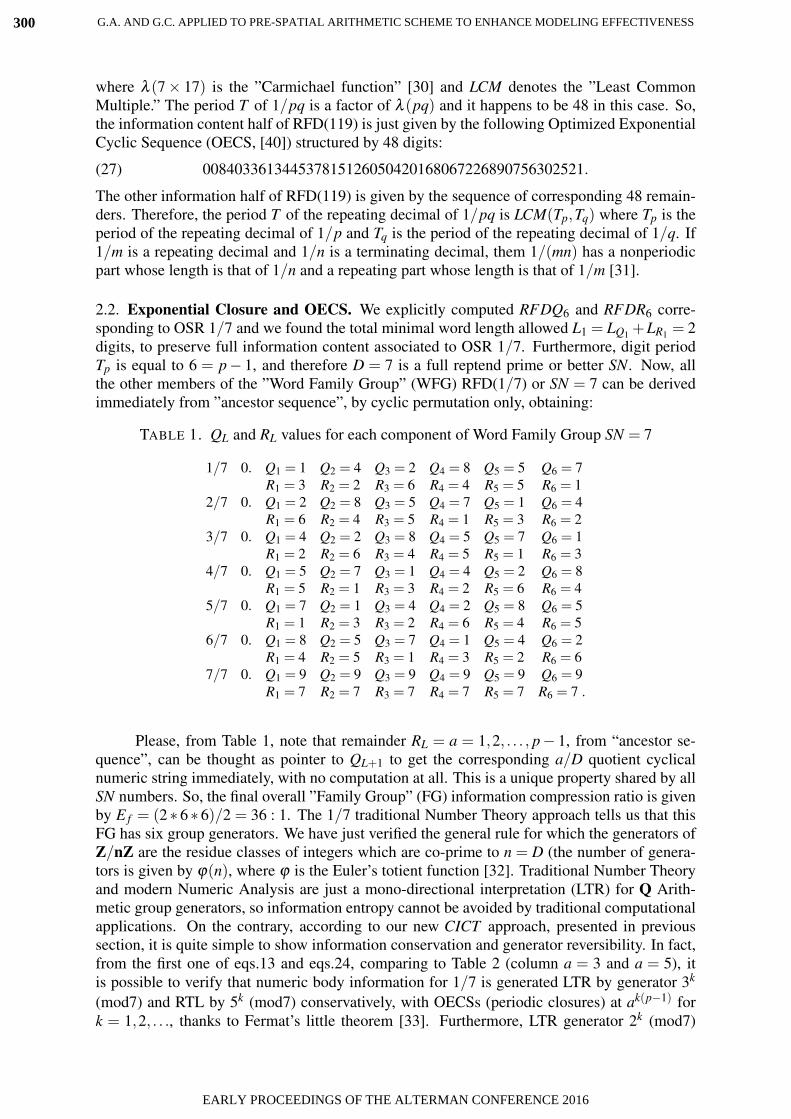
where λ (7 × 17) is the ”Carmichael function” [30] and LCM denotes the ”Least CommonMultiple.” The period T of 1/pq is a factor of λ (pq) and it happens to be 48 in this case. So,the information content half of RFD(119) is just given by the following Optimized ExponentialCyclic Sequence (OECS, [40]) structured by 48 digits:

(27) 008403361344537815126050420168067226890756302521.

The other information half of RFD(119) is given by the sequence of corresponding 48 remain-ders. Therefore, the period T of the repeating decimal of 1/pq is LCM(Tp,Tq) where Tp is theperiod of the repeating decimal of 1/p and Tq is the period of the repeating decimal of 1/q. If1/m is a repeating decimal and 1/n is a terminating decimal, them 1/(mn) has a nonperiodicpart whose length is that of 1/n and a repeating part whose length is that of 1/m [31].

2.2. Exponential Closure and OECS. We explicitly computed RFDQ6 and RFDR6 corre-sponding to OSR 1/7 and we found the total minimal word length allowed L1 = LQ1 +LR1 = 2digits, to preserve full information content associated to OSR 1/7. Furthermore, digit periodTp is equal to 6 = p− 1, and therefore D = 7 is a full reptend prime or better SN. Now, allthe other members of the ”Word Family Group” (WFG) RFD(1/7) or SN = 7 can be derivedimmediately from ”ancestor sequence”, by cyclic permutation only, obtaining:

TABLE 1. QL and RL values for each component of Word Family Group SN = 7

1/7 0. Q1 = 1 Q2 = 4 Q3 = 2 Q4 = 8 Q5 = 5 Q6 = 7R1 = 3 R2 = 2 R3 = 6 R4 = 4 R5 = 5 R6 = 1

2/7 0. Q1 = 2 Q2 = 8 Q3 = 5 Q4 = 7 Q5 = 1 Q6 = 4R1 = 6 R2 = 4 R3 = 5 R4 = 1 R5 = 3 R6 = 2

3/7 0. Q1 = 4 Q2 = 2 Q3 = 8 Q4 = 5 Q5 = 7 Q6 = 1R1 = 2 R2 = 6 R3 = 4 R4 = 5 R5 = 1 R6 = 3

4/7 0. Q1 = 5 Q2 = 7 Q3 = 1 Q4 = 4 Q5 = 2 Q6 = 8R1 = 5 R2 = 1 R3 = 3 R4 = 2 R5 = 6 R6 = 4

5/7 0. Q1 = 7 Q2 = 1 Q3 = 4 Q4 = 2 Q5 = 8 Q6 = 5R1 = 1 R2 = 3 R3 = 2 R4 = 6 R5 = 4 R6 = 5

6/7 0. Q1 = 8 Q2 = 5 Q3 = 7 Q4 = 1 Q5 = 4 Q6 = 2R1 = 4 R2 = 5 R3 = 1 R4 = 3 R5 = 2 R6 = 6

7/7 0. Q1 = 9 Q2 = 9 Q3 = 9 Q4 = 9 Q5 = 9 Q6 = 9R1 = 7 R2 = 7 R3 = 7 R4 = 7 R5 = 7 R6 = 7 .

Please, from Table 1, note that remainder RL = a = 1,2, . . . , p− 1, from “ancestor se-quence”, can be thought as pointer to QL+1 to get the corresponding a/D quotient cyclicalnumeric string immediately, with no computation at all. This is a unique property shared by allSN numbers. So, the final overall ”Family Group” (FG) information compression ratio is givenby E f = (2 ∗ 6 ∗ 6)/2 = 36 : 1. The 1/7 traditional Number Theory approach tells us that thisFG has six group generators. We have just verified the general rule for which the generators ofZ/nZ are the residue classes of integers which are co-prime to n = D (the number of genera-tors is given by ϕ(n), where ϕ is the Euler’s totient function [32]. Traditional Number Theoryand modern Numeric Analysis are just a mono-directional interpretation (LTR) for Q Arith-metic group generators, so information entropy cannot be avoided by traditional computationalapplications. On the contrary, according to our new CICT approach, presented in previoussection, it is quite simple to show information conservation and generator reversibility. In fact,from the first one of eqs.13 and eqs.24, comparing to Table 2 (column a = 3 and a = 5), itis possible to verify that numeric body information for 1/7 is generated LTR by generator 3k

(mod7) and RTL by 5k (mod7) conservatively, with OECSs (periodic closures) at ak(p−1) fork = 1,2, . . ., thanks to Fermat’s little theorem [33]. Furthermore, LTR generator 2k (mod7)



corresponds to LTR generator 4k (mod7), with half-cycle period, and generator 6k (mod7) isself-corresponding alternately to unity. FG 1/7 contains the smallest cyclic-numbers of orderone, shown manifestly. Next larger prime number p to show SN property might be a good

TABLE 2. Modular Power a (mod7)

Number a 01 02 03 04 05 06 07 08Power Order

01 01 02 03 04 05 06 00 0102 01 04 02 02 04 01 00 0103 01 01 06 01 06 06 00 0104 01 02 04 04 02 01 00 0105 01 04 05 02 03 06 00 0106 01 01 01 01 01 01 00 01

SubCycle 06 02 01 02 01 03 00 06

candidate for exhibiting cyclic-number property on an even larger scale. Unfortunately theredoes not seem to be any simple rule dictating which prime number p will have SN property andwhich will not, so that one just has to check each prime out by long division to see. It turns outthat the next higher prime number with the desired SN property is p = D = 17 where Tp = 16digits. A search for still larger prime numbers reveals that they are not at all rare. In fact noless than seven more prime numbers smaller than 100 generate cyclic numbers of order one orSN. They are: 19,23,29,47,59,61 and 97. So, what about OSR when D is not SN? In thatcase LX is the result of the exponential modular interplay with D and 10k (modD). Let us seea simple example. Let us consider a prime p , after 7. In this case p = D = 13, with Tp = 6,and 10k (mod13) gives the following repeating sequence (10,09,12,03,04,01) with cycle sixfor remainders. Therefore, even in this case LX = 6 digits like for 1/7, but 10k (mod13) it isnot a full sequence generator, this time (see Table 3, column a = 10). One cycle six is sufficientto characterize half ”Family Members” (FMs) only, this time. In fact, in the obtained sequenceonly six terms for the counting sequence from 01 to (D−1) = 12 are present. What about theother half FMs? It is immediate to find that they are given by 2 ∗ 10k (mod13) with the fol-lowing repeating sequence (07,05,11,06,08,02) for remainders, with cycle six again. Finallywe got all the terms! So 1/13 WFG presents a RFD structure split into two prime subdomains(1/13 and 2/13) both with Tp = 6. Therefore D = 13 is a SN of order 2, or SN2 for short.Now, from Table 3, it is manifest that inner RFDs can be thought as structured combinatorical

TABLE 3. Modular Power a (mod13)

Number a 01 02 03 04 05 06 07 08 09 10 11 12 13 14Power Order

01 01 02 03 04 05 06 07 08 09 10 11 12 00 0102 01 04 09 03 12 10 10 12 03 09 04 01 00 0103 01 08 01 12 08 08 05 05 01 12 05 12 00 0104 01 03 03 09 01 09 09 01 09 03 03 01 00 0105 01 06 09 10 05 02 11 08 03 04 07 12 00 0106 01 12 01 01 12 12 12 12 01 01 12 01 00 0107 01 11 03 04 08 07 06 05 09 10 02 12 00 0108 01 09 09 03 01 03 03 01 03 09 09 01 00 0109 01 05 01 12 05 05 08 08 01 12 03 12 00 0110 01 10 03 09 12 04 04 12 09 03 10 01 00 0111 01 07 09 10 08 11 02 05 03 04 06 12 00 0112 01 01 01 01 01 01 01 01 01 01 01 01 00 01

SubCycle 12 01 04 02 03 01 01 03 04 02 01 06 00 12

optimizations of their FG generators to achieve full information content conservation by power



modular reversibility (LTR and RTL). Again, from Table 3, it is possible to verify immedi-ately that numeric body information for family subgroup 1/13 is generated LTR by generator10k = 62k = 72k (mod13) and RTL by 4k = 22k = 112k (mod13) conservatively, with expo-nential periodic closure at ak(p−1)/2 for k = 1,2, . . .. Furthermore, LTR generator 9k (mod13)corresponds to LTR generator 3k (mod13), with four subcycles, and generator 12k (mod13) isself-corresponding alternately to unity (to get a periodic word with one mapped ”fixed point”at 12). Numeric body information for family subgroup 2/13 is generated LTR by generator 7k

(mod13) and RTL by 2k (mod13) conservatively, with exponential periodic closure at ak(p−1)

for k = 1,2, . . .. Furthermore, LTR generator 5k (mod13) corresponds to RTL generator 8k

(mod13), with three subcycles, and LTR generator 11k (mod13) corresponds to LTR generator6k (mod13), (to get a periodic word with a mapped ”pairing”). Actually, since space is lim-ited, the discussion here will not be extended to the subgroup interplay of the family groupand polycyclic groups. Good general references on polycyclic groups are [34, 35]. Word innergenerator combinatorical structure can be arranged for ”pairing” and ”fixed point” propertiesfor digit group with the same word length. As a matter of fact, those properties (”pairing” and”fixed point”) are just the operational manifestation of universal categorical dichotomy hard-wired into integer digit and digit group themselves (evenness and oddness, correspondence andincidence fundamental discrete relations). So, FG 1/13 contains the smallest numeric cyclic-words of order two. What about more second order SN FGs? The basic ones are also generatedby a subset of prime fractions 1/p. The other prime numbers smaller than 100 which gen-erate second order SN FG are 31,43,67,71,83 and 89. In the same manner one can now goon to define, and find, SN FG of order three, four, five, and higher and higher, according tocomputational needs. The smallest prime number producing third order SN FG is 103. In thiscase, Tp = 34 digits (instead of 102 digits a first order SN FG would have). The seven small-est primes generating SN FGs of order four through ten are respectively 53,11,79,211,41,73,and 281, but you must reach prime number 353 to get the first SN FG of order 11. All theprime numbers less than 100 have now been covered with the exception of p = 37, with Tp = 3digits. Therefore 37 is a SN FG of order 12. Till now we discussed peculiar number prop-erty focusing our attention, for simplicity of presentation, on prime numbers only, but we donot wish to imply that a number has to be a prime in order to generate intriguing cycles. Wealready saw, briefly, that multiplication composition of prime numbers can generate an entireuniverse of new number-cycles. The decimal forms of quite arbitrary fractions nearly alwayshave some unexpected fascination in their cycling behaviour. For example, consider FG (1/21)with Tp = 6, or FG (1/39) with Tp = 6, or FG (1/63) with Tp = 6, or FG (1/91) with Tp = 6again!

3. CICT PG ALL-POWERFUL FRAMEWORK

CICT [36] new awareness of a discrete HG (hyperbolic geometry) subspace (”Reciprocal-Space”, RS) of coded heterogeneous hyperbolic structures [43], underlying the familiar Q Eu-clidean ”Direct-Space” (DS) surface representation, shows that any natural number n in N hasassociated a specific, non-arbitrary extrinsic or external phase relationship that we have to takeinto account to full conserve overall system component information content by computationin DS [37]. Recently, CICT has shown that, by Shannon entropy approach only, even thecurrent, most sophisticated instrumentation system is completely unable to reliably discrimi-nate so called ”Random Noise” (RN) from any combinatorically optimized encoded message,which CICT called ”Deterministic Noise” (DN) [13]. Stochastic vs. combinatorically op-timized noise generation ambiguity emphasises the major ”Information Double-Bind” (IDB)problem even in current most advanced research laboratory and instrumentation system, justat the inner core of human knowledge extraction by experimentation in contemporary science[13]. CICT solved the IDB problem by ”Phased Generator” (PG) approach. CICT is a natural



framework for arbitrary multi-scale (AMS) computer science, biophysical and systems biologymodelling in the current landscape of modern QFT [38, 39], created to overcome the compu-tational limitations focused in previous sections. Thanks to this line of generative thinking, itis possible to realize that traditional rational number system can be even regarded as a highlysophisticated open logic, powerful and flexible LTR and RTL formal language of languages,with self-defining consistent words and rules, starting from elementary generators and relations[13]. Further, CICT ODR (Observation, Description, Representation) approach [40] can takeadvantage immediately from those properties to develop system computational functional clo-sures to achieve information conservation countermeasure at each operative step automatically.Then, all computational information usually lost by classic information approach, based on thetraditional noise-affected data stochastic model only, can be captured and fully recovered toarbitrary precision by a corresponding complementary codomain, step-by-step. Theoretically,codomain information can be used to correct any computed result, achieving computationalinformation conservation (virtually noise-free data), according to CICT Infocentric Worldview[13]. In this way, overall system resilience and antifragility can be developed quite easily[41]. In fact, traditional digital computational resources are unable to capture and to managenot only the full information content of a single Real Number R, but even Rational NumberQ is managed by information dissipation. In numeric representation of Rational Number Q,rational proper quotient is represented by infinite repetition of a basic digit cycle, called ”rep-tend” (the repeating decimal part) [27]. According to CICT , the first repetition of basic digitcycle corresponds to the first full scale interval where number information can be conservedcompletely, and we call it RFD. In this case the new computational representation of rationalnumber Q, is called ”OpeRational Representation” (OR), just to remember that CICT is ableto conserve Rational Number Q full information content, much better than previous computa-tional approaches. CICT sees natural integers N as specific numeric resonances emerging outof the OECS (optimized exponential cyclic sequence) [40] manifold of rational values Q. Inturn, OECS can be thought emerging out from the peculiar numeric resonances of irrationalnumeric sequences generated by DS-RS coherent cross-interaction with their duals, accordingto the following two algebraic identities:

(28)1D

=1

( M√

D)P· 1( M√

D)(M−P)=

1

DPM·D P−M

M ,

for P > 0 and M ≥ P = 1,2, . . . ,∞, where D ∈Q; and

(29)1D

= (M√

D)P · 1( M√

D)(M+P)= D

PM · 1

DM+P

M,

for P < 0. DS-RS cross-interaction with their duals is assumed to be our spacetime represen-tation fundamental property. Eventually, CICT OECSs have strong connection even to clas-sic DFT algorithmic structure for discrete data, Number-Theoretic Transform (NTT), Laplaceand Mellin Transforms [13]. Coherent precision correspondence (numeric resonance) leads totransparency, ordering, reversibility, cosmos, simplicity, clarity, and to algorithmic quantumincomputability on real macroscopic machines [37]. CICT natural framework is quite flexi-ble and can be used under two major operational representation schemes: ”Formal RecurrenceSequence (FRS) in Section 3.1, and ”Formal Power Series” (FPS) (Section 3.2) presentation,respectively.

3.1. CICT FRS Presentation. CICT can be presented and used in term of recurrence relation.In this case, rational geometric series can be seen as simple recurrence sequences in a wider re-currence operative framework where all algebraic recurrence sequences of any countable higherorder include all the lower order ones and they can be optimally mapped to rational number sys-tem Q ORs and generating functions to OECS [40]. For instance, arithmetic progression and



Lucas sequences are recurrence sequences of the second order. Lucas sequences are certaininteger sequences that satisfy Lucas recurrence relation defined by polynomials Un(P,Q) andVn(P,Q), where Un, Vn are specific polynomials and P, Q are fixed integer coefficients.[23] Anyother sequence satisfying this recurrence relation can be represented as a linear combination ofthe Lucas sequences Un(P,Q) and Vn(P,Q). Famous examples of Lucas sequences include theFibonacci numbers, Mersenne numbers, Pell numbers, Lucas numbers, Jacobsthal numbers,and a superset of Fermat numbers. CICT is able to fold any recursion sequence of the firstorder into one digit number D, any recursion sequence of second order into a two digit numberD, any recursion sequence of the third order into a three digit number D and so on to higherorders. Then, you can compute their asymptotic convergence velocities as related roots fromcorresponding first, second, third, etc. . . , order equations respectively. In papers presentedelsewhere, the interested reader can go deeper into CICT FRS presentation main properties[23, 43].

3.2. CICT FPS Presentation. Basic CICT result can be even presented in term of classicmonopolar power series, or in general by formal power series, to show the close relationshipsto classic and modern control theory approaches for causal continuous-time and discrete-timelinear systems. The CICT fundamental relationship that ties together numeric body informationof RTL to RTL monotonic power series in any base (in this case decimal, with no loss ofgenerality) with D ending by digit 9 is given by the following equation:

(30)1D

=∞

∑k=0

110W

(D

10W

)k

⇒ ·· · ⇐ Div(

1D

)=

∞

∑k=0

(D+1)k ,

where D is the additive 10W complement of D, i.e. D = (10W −D), W is the word representa-tion precision length of the denominator D and ”Div” means ”Divergence of”. When D > D theformal power series on the left of eq.30 can be re-scaled modD, to give multiple convergencepaths to 1/D, but with different ”convergence speeds.” The total number of allowed convergentpaths, as monotonic power series, is given by the corresponding QL value, at the consideredaccuracy level. So, increasing the level of representation accuracy, the total number of allowedconvergent paths to 1/D, as monotonic power series (as allowed conservative paths), increasesaccordingly and can be counted exactly, and so on, till maximum machine word length andbeyond: like discrete quantum paths denser and denser to one another, towards a never ending”blending quantum continuum,” by a top-down perspective. By using this approach, it is possi-ble to generate LTR and RTL remainder sequences that show same quotient body information(multi-scale periodic) and specific quotient head and tail information to compute deterministicboundary values, to sustain body periodicity with no information dissipation (full informationconservation and reversibility) [25]. Further generalizations of right term of eq.30 related to Dending by digit 1 or 3 or 7 are straightforward. In fact, we can re-write the right term of eq.30as:

(31) Div(

1D

)=

∞

∑k=0

Gk,

where G is a specific RTL generator. Then, it is immediate to verify that for G = (9D+ 1),G = (3D+1) and G = (7D+1) the RTL periodic string will match the LTR one generated by:

(32)1D

=∞

∑k=0

110W

(D

10W

)k

.

It will match exactly the sequences generated by number word D of length W , right endingby digit 1 or 3 or 7 respectively. As monotonic power series (as allowed subspace paths), byincreasing the subspace representation accuracy, the total number of allowed convergent pathsincreases accordingly till maximum machine word length and beyond; like discrete quantum



paths denser and denser to one another, towards never ending ”blending quantum continuum,”called ”quantum mixture” by current FMM (Finite Mixture Model) top-down statistical pointof view for composite AMS system, as we discussed in previous section. On the contrary, forCICT the finer geometry of subspace itself becomes scale dependent. While differentiable tra-jectories found in standard mathematical physics are automatically scale invariant, it is the maininsight of the CICT theory that also certain non-differentiable paths (resultant paths, emergingfrom lower scales combined quantum trajectory interactions, which explicitly depend on thescale and accuracy of the observer) can be scale invariant. Rational representations are ableto capture two different types of information at the same time, modulus (usual quotient in-formation) and associated outer or information period (extrinsic phase, represented by RFD[25]) which an inner, or intrinsic phase can be computed from. So, rational information can bebetter thought to be isomorphic to vector information rather than to usual scalar one, at least.According to Hestenes [8], we can take the mathematical concepts of modular magnitude anddirection as basic, and introduce the concept of vector as the basic kind of directed number, withan additional, associated, specific phasing relation. Directed numbers are defined implicitly byspecifying rules for adding and multiplying vectors. According to CICT vector representationprecision, directed numbers (modular magnitude and direction) can be related uniquely to longdivision rational remainder sequences to identify convenient ”quantum support field” relations,which subspace inner phased generators can be computed from. Furthermore, our knowledgeof RFDQL and corresponding RFDRL can allow reversing numeric power convergent sequenceto its corresponding numeric power divergent sequence uniquely [25]. Reversing a convergencesequence to a divergence one and vice-versa is the basic property to reach information conser-vation, i.e. information reversibility, as from eq.30. For future reference, it is convenient to usea compact notation for LTR geometric series as follows:

(33)1D

=∞

∑k=0

N10W

(CR10W

)k

≡ NW (CRW ),

where D is denominator, N numerator, CR power series constant ratio, and W the length of theirdigit strings. Then, it is immediate to verify that at W = 1 (accuracy = 10−1), unity can emergeout of a fundamental symmetrical multiplicity of different monopolar countable paths, but withdifferent ”convergence speeds” (in this case 9):

1(9) ≡ 1/1, (8) ≡ 1/1, 3(7) ≡ 1/1, 4(6) ≡ 1/1, 5(5) ≡ 1/1, 6(4) ≡ 1/1, 7(3) ≡ 1/1,8(2)≡ 1/1, 9(1)≡ 1/1.

At W = 2 (accuracy = 10−2, therefore 99 different monopolar countable paths), we have:01(99) ≡ 1/1, 02(98) ≡ 1/1, 03(97) ≡ 1/1, 04(96) ≡ 1/1, 05(95) ≡ 1/1, . . ., 96(04) ≡ 1/1,97(03) ≡ 1/1, 98(02) ≡ 1/1, 99(01) ≡ 1/1.

At W = 3 (accuracy = 10−3, therefore 999 different monopolar countable paths), wehave: 001(999) ≡ 1/1, 002(998) ≡ 1/1, 003(997) ≡ 1/1, 004(996) ≡ 1/1, 005(995) ≡ 1/1,. . ., 996(004) ≡ 1/1, 997(003) ≡ 1/1, 998(002) ≡ 1/1, 999(001) ≡ 1/1, and so on for W = 4,5, . . ., W ∈ N. The interested reader to go deeper into CICT FPS presentation is referred to[13, 25, 40, 42]

4. RECOVERING THE EXTERIOR PHASE RELATIONSHIP

To conserve the full ST information content, we need to avoid the loss of overall sys-tem fundamental information (the pre-splitting information phase loss, connecting time com-ponent to space component coherently into their primitive spacetime continuum field F , attheir original gauge level), which is manifestly an ill-posed problem by classic scientific ap-proach (Science 1.0). CICT new awareness of the discrete HG (hyperbolic geometry) based



RS of coded heterogeneous hyperbolic structures [36], underlying the familiar Q Euclidean DSsurface representation can open the way to AMS information conservation by the CICT PGapproach [13, 25]. First, let us introduce the LTR ”Symbolic Compression Operator” SCO ≡< M | DS >, where DS is a finite digit string of length W and M is the number of times DS isrepeated to get the final unfolded digit string in full (e.g. < 4 | 1 > ≡ 1111 or < 2 | 123 > ≡123123). Usual symbolic string operations can be applied to SCO. Then, we can write usualrational number OR corresponding to their symbolic representation as [25]:

(34)

Q1 =1

D1= 1

9 = ∑∞k=0

1101

(1

101

)k= 0.11111111111111111 . . .

Q2 =1

D2= 1

99 = ∑∞k=0

01102

(1

102

)k= 0.01010101010101010 . . .

Q3 =1

D3= 1

999 = ∑∞k=0

001103

(1

103

)k= 0.00100100100100100 . . .

. . . . . . ,

in a more compact RFD, [25] QW format as:

(35)

Q1 =1

D1= 1

9 ≡ 0. < ∞|1 >= 0. < ∞|(< 0 | 0 >< 1 | 1 >)>

Q2 =1

D2= 1

99 ≡ 0. < ∞|01 >= 0. < ∞|(< 1 | 0 >< 1 | 1 >)>

Q3 =1

D3= 1

999 ≡ 0. < ∞|001 >= 0. < ∞|(< 2 | 0 >< 1 | 1 >)>

.. . . . .Qn =

1Dn

≡ 1<n|9> = 0. < ∞|(< n | 0 >< 1 | 1 >)>

.. . . . .

In the same way, we can write:

(36)

P1 =1

DD1= 1

1 = ∑∞k=0

9101

(1

101

)k= 0.99999999999999999 . . .

P2 =1

DD2= 1

11 = ∑∞k=0

09102

(1

102

)k= 0.09090909090909090 . . .

P3 =1

DD3= 1

111 = ∑∞k=0

009103

(1

103

)k= 0.00900900900900900 . . .

. . . . . .P1 =

1DD1

= 11 ≡ 0. < ∞|9 >= 0. < ∞|(< 0 | 0 >< 1 | 9 >)>

P2 =1

DD2= 1

11 ≡ 0. < ∞|09 >= 0. < ∞|(< 1 | 0 >< 1 | 9 >)>

P3 =1

DD3= 1

111 ≡ 0. < ∞|009 >= 0. < ∞|(< 2 | 0 >< 1 | 9 >)>

.. . . . .Pn =

1DDn

≡ 1<n|1> = 0. < ∞|(< n | 0 >< 1 | 9 >)>

.. . . . .

Now, we can realize that P1 RFD is related by Q1 RFD, P2 RFD is related by Q2 RFD, P3 RFDis related by Q3 RFD,. . . and vice-versa by periodic scale relativity (precision length) W = 1,2, 3, . . . , respectively. So, to conserve the full information content of rational correspondencebetween Q1 and P1, Q2 and P2, Q3 and P3, . . . , we realize that we have to take into account notonly the usual Q1 and P1, etc., modulus information, but even their related periodic precisionlength information W = 1, 2, 3, . . . , respectively (external or extrinsic phase representation).Furthermore we see that:

(37)

O1 =1

DDD1= 1

9 ≡ 0. < ∞|1 >= 0. < ∞|(< 1 | 1 >)>

O2 =1

DDD2= 1

09 ≡ 0. < ∞|11 >= 0. < ∞|(< 2 | 1 >)>

O3 =1

DDD3= 1

009 ≡ 0. < ∞|111 >= 0. < ∞|(< 3 | 1 >)>

.. . . . .On =

1DDDn

≡ 1(<n|0><1|9>) = 0. < ∞|(< n | 1 >)>

.. . . . .



The coherent representations DDD1, DDD2, DDD3, etc. emerge out of a LTR infinity of sym-bolic structured infinite length sequences as in eq.37. So, DDDn is the coherent relation repre-sentation of traditional scalar modulus D1 in eq.34 as denominator at precision W , while scalarmodulus D1 in eq.34 has to be interpreted as the decoherenced relation representation of DDDndenominators in eq.37. In general, for any Natural number D ∈ N we can write:

(38)1

< n | RFD(D)>≡≡< (< k+W (n−1) | 0 >< 1 | D >)> .

< (< k+W (n−1) | 0 >< 1 | D >)>,

where RFD is at precision W and k is the number of leading zeros in RFD (if any) at precisionW . Now, for n → ∞, we get:

(39)1

< n | RFD(D)>≡≡< (< k+W (∞−1) | 0 >< 1 | D >)> .

< (< k+W (∞−1) | 0 >< 1 | D >)>= 0D.0.

Then, Natural numbers N emerge from eq.39 as a conceptual abstraction, just as the rightmostapproximated part of those LTR structured sequences when n → ∞, for n ∈ N, with left trun-cated decimal part (represented by leading zeroes on any finite computational machine). In thisway we loose the basic coherence relationship with its fundamental string generators (i.e. infor-mation dissipation and system decoherence) completely. Leading zeros in positional notationrepresentation system for CICT Q Arithmetic do count effectively, and can model the systemquantum-classical transition quite effectively [23]. If we do not take into account leading zerosinformation, we lose the correct rational RFD correspondence information (coherence) whichan outer or extrinsic phase for each RTL (right-to-left) string generator can be computed from(i.e. from their optimized exponential cyclic sequences (OECS) of RW [37]) first. Therefore,Rational numeric representations are able to capture two different types of information at thesame time, modulus (usual quotient information) and RFD associated information period (ex-terior or external or extrinsic phase, EP), which inner generator intrinsic period (interior orinternal or intrinsic generator phase, IP) can be computed from. So, rational information can bebetter thought to be isomorphic to vector information rather than to usual scalar one, at least.As an example, according to our SCO approach, the correct coherent relation representation oftraditional scalar modulus D = 07.0 as denominator of Egyptian fraction, is given by:

(40) CQ1 =1

CD1≡ 1

< ∞ | (< ∞ | 0 >< 1 | 7 >)>≡

≡ 0. < ∞|RFD(7)>≡ 0. < ∞|142857 > .

Therefore, to conserve the full information content of rational correspondence at higher level,we realize that we have to take into account not only the usual modulus information, but eventhe related periodic precision length information W = 6 (numeric period or external phaserepresentation) in this case (i.e. CD1 = 000007 as base RFD). We can use Euler’s formula toestablish the usual fundamental relationship between trigonometric functions and the complexexponential function:

(41) eix = cosx+ isinx,



where e is the natural mathematical constant and i =√−1. The final result is:

(42) CQQ1 =1

CDD1=

17

ei π(2n+1)3 =

17(cos(

2π(n+1)6

)+ isin(2π(n+1)

6))

and

(43) CDD1 =1

CQQ1= 7(e−i π(2n+1)

3 ) = 7(cos(π(2n−1)

3)+ isin(

π(2n−1)3

)) =

= 7(12− i

√3

2) (p.v.)

for n = 0, 1, 2, 3, ...in N, where (p.v.) means ”principal value”. CICT shows that any naturalnumber D ∈ Q has associated a specific, non-arbitrary external phase relationship (OptimizedExponential Cyclic Sequence, OECS, coherence information, [40]) that we must take into ac-count to conserve its full information content by computation in Euclidean space [36]. Thecareful reader will have already guessed the relationship of our result to de Moivre number orroot of unity (i.e. any complex number that gives 1.0 when raised to some integer power of n).In this way, we can exploit rational numbers Q full information content to get stronger solu-tions to current AMS system modeling problems [12], by keeping their information coherence.Our RFD period knowledge associated to specific rational number D reveals its associated EPinformation immediately. From EP, CICT allows to compute each RFD inner generator IP togo through the statistical modeling veil opacity, by phased generator approach, as you alreadysaw in Section 2. This result, offered by 1/D rational remainder sequence, can be interpretedas the optimized combination of elementary quantum phase irrational fluctuations.

5. CONCLUSION

In arbitrary multiscale complex system modelling the bottom-up discrete approach un-der the ”discreteness hypothesis” is mandatory to achieve effective solutions. In fact, CICTshows that any natural number D ∈ N has associated a specific, non-arbitrary external phaserelationship (OECS coherence information, [40]) that we must take into account to full con-serve its information content by computation in Euclidean DS [36]. RFD period knowledgeassociated to specific rational number D reveals its EP information immediately. From EP,CICT allows to compute each RFD inner generator IP to tear aside or minimize the traditionalprobabilistic modeling veil opacity. CICT achieves this result by 1/D rational remainder se-quence, interpreted as optimized combination of elementary quantum phase generators. There-fore, to conserve the full information content of rational correspondence at higher level, werealize that we have to take into account not only the usual modulus information, but even therelated RFD periodic precision length information. According to QFT, the gauge invariancein quantum physics becomes the natural partner of the phase invariance to produce the rep-resentation and description of our world. Quantum fluctuations give rise to electromagneticpotentials which spread the phase fluctuations beyond the system at the phase velocity. Thisgives an intrinsic nonlocalizability to the system and prevents a direct observation of quantumfluctuations. Through the electromagnetic potential, the system gets a chance to communicatewith other systems and subsystems [42]. QFT has emerged from a major ontological para-digm shift with respect to Classical Physics which still provides the traditional framework ofthe vision of nature of most ”Science 1.0” current scientists. This change of paradigm has notyet been completely grasped at operative level in full by many contemporary scientists andresearchers in different disciplined areas, so that not all the implications of this change havebeen realized hitherto, even less their related applications. So, the discreteness approach, de-veloped under the ”discreteness hypothesis” assumption, in specific scientific disciplines, hasbeen considered in peculiar application areas only. It has been further slowly developed by



a few specialists and less understood by a wider audience. Unfortunately, over the centuries,the two large scientific research areas (continuum based and discreteness based) have followedseparate mathematical development paths with no or quite little, inconsistent synergic coupling.That is the main reason why QFT is still mostly overlooked by traditional scientific and engi-neering researchers for arbitrary multi-scale system modelling, from system nano-microscaleto macroscale. Reversing a convergent sequence into a divergent one and vice-versa is thefundamental property to reach information conservation, i.e. information reversibility. Eventu-ally, CICT OECS have strong connection even to classic DFT algorithmic structure for discretedata, Number-Theoretic Transform (NTT), Laplace and Mellin Transforms [12]. As a matterof fact, to grasp a more reliable representation of reality, researchers and scientists need twointelligently articulated hands; both stochastic and combinatorical approach synergistically ar-ticulated by natural coupling; let’s say we need a fresh ”Science 2.0” approach [42]. CICTcombined to GA and GC unified mathematical language can offer an effective and convenient”Science 2.0” universal framework, by considering information not only on the statistical man-ifold of model states but also on the combinatorical manifold of low-level discrete, phasedgenerators and empirical measures of noise sources, related to experimental high-level overallperturbation. It is the fresh QFT approach. CICT coherent precision correspondence allowsus to tear aside or minimize the probabilistic veil reaching transparency, ordering, reversibil-ity, cosmos, simplicity and clarity, by a simple arithmetic scheme strongly coupled to GA andGC representations [44]. This paper is a relevant contribution towards an effective and conve-nient ”Science 2.0” universal framework to develop more effective biophysics modelling andsimulation for competitive application and beyond [45].

ABBREVIATIONS

AMS: Arbitrary Multi-ScaleCA: Clifford AlgebraCICT: Computational Information Conservation TheoryDN: Deterministic NoiseDS: Direct-SpaceEP: Exterior or External or Extrinsic PhaseFCRS: Fundamental Cyclic Remainder SequenceFCQS: Fundamental Cyclic Quotient SequenceFG: Family FroupFM: Family MemberFPS: Formal Power SeriesFRS: Formal Recurrence SequenceGA: Geometric AlgebraGC: Geometric CalculusIDB: Information Double-BindIO: Inertial ObserverIOR: Inner OpeRational RepresentatioIP: Interior or Internal or Intrinsic PhaseLCM: Least Common MultipleLTR: Left-To-RightNTT: Number-Theoretic TransformODR: Observation, Description, RepresentationOECS: Optimized Exponential Cyclic SequenceOR: OpeRationalOSR: Outer Symbolic RepresentationPG: Phased Generator



QFT: Quantum Field TheoryQM: Quantum MechanicsRFD: Representation Fundamental DomainRN: Random NoiseRS: Reciprocal SpaceRTL: Right-To-LeftSN: Solid NumberST: SpacetimeSTA: Space-Time AlgebraWFG: Word Family Group

REFERENCES

[1] W. Heisenberg, Die physikalischen Prinzipien der Quantentheorie, (S. Hirzel, Leipzig, 1941).[2] D. Hestenes and G. Sobczyk, Clifford Algebra to Geometric Calculus, a Unified Language for Mathematics

and Physics, G. Reidel Publ. Co. (Dordrecht/Boston, 1984, paperback, 1985, third printing, 1992).[3] D. Hestenes, Spacetime Algebra, Gordon and Breach (New York, 1966).[4] G. Ghirardi, Sneaking a Look at God’s Cards: Unraveling the Mysteries of Quantum Mechanics, Malsbary

G. (translator), Princeton University Press (Princeton, NJ, 2007).[5] E. Del Giudice and G. Preparata, ”Coherent dynamics in water as a possible explanation of biological

membranes formation”, Journal of Biological Physics 20 (1995) 105—116.[6] M. Bischof and E. Del Giudice, ”Communication and the Emergence of Collective Behavior in Living

Organisms: A Quantum Approach”,Molecular Biology International Article ID 987549 (2013) 19 pages.,DOI: http://dx.doi.org/10.1155/2013/987549.

[7] D. Hestenes, ”Spacetime physics with geometric algebra”, Amer. J. Phys. 71 (2003) 1–24.[8] D. Hestenes, New Foundations for Classical Mechanics, D. Reidel Pub. Co. (Dordrecht, Holland, 1986).[9] The NIST Reference on Constants, Units and Uncertainty, Unit of electric current (ampere) (2015), avail-

able at http://physics.nist.gov/cuu/Units/ampere.html.[10] R. A. Fiorini, ”Entropy, Decoherence and Spacetime Splitting”, Proceedings of the 2nd Int. Electron. Conf.

Entropy and Its Appl. (15–30 November 2015), Sciforum Electronic Conference Series, 2 (2015) A003,doi:10.3390/ecea-2-A003, available at http://sciforum.net/conference/ecea–2/paper/3176.

[11] E. B. Wilson and G. N. Lewis, ”The space-time manifold of relativity. The non-Euclidean geometry ofmechanics and electromagnetics”, Proc. Amer. Acad. Arts Sci. 48 (1912) 387–507.

[12] A. Aste, ”Complex representation theory of the electromagnetic field”, Journal of Geometry and Symmetryin Physics 28 (2012) 47–58.

[13] R. A. Fiorini, ”How Random is Your Tomographic Noise? A Number Theoretic Transform (NTT) Ap-proach”, Fundamenta Informaticae 135 (2014) 135–170.

[14] Y. P. Stepanovsky, ”From Maxwell equation to Berry’s phase and sonoluminescence: Problems of theoryof electromagnetic and other Massless fields”, Electromagnetic Phenomena 1 (1998) 180–218.

[15] D. H. Kobe, ”A relativistic Schrodinger-like equation for a photon and its second quantization”, Found.Phys. 19 (1999) 1203–1231.

[16] J. B. Smith and M. G. Raymer, ”Photon wave functions, wave-packet quantization of light, and coherencetheory”, New J. Phys. 19 (2007) 414.

[17] D. Dragoman, ”Photon states from propagating complex electromagnetic fields”, J. Opt. Soc Am. B24(2007) 922–927.

[18] F. Tamburini and D. Vicino, ”Photon wave function: A covariant formulation and equivalence with QED”,Phys. Rev. A 8 (2008) 052–116.

[19] B. Thide, Electromagnetic Field Theory, Dover Publications (New York, NY, 2014).[20] B. Thide, The physics of angular momentum radio, reprint (2015), available at http://arxiv.org/pdf/1410.4268.[21] J. Dressel, K. Y. Bliokh, F. Nori, Spacetime algebra as a powerful tool for electromagnetism. Phys.Rept.

589 2015, 1–71.[22] H. Grassmann, Die Lineale Ausdehnungslehre — Ein neuer Zweig der Mathematik, Verlag von Otto Wigand

(Leipzig, 1844).[23] R.A. Fiorini, ”Arbitrary Multi-Scale (AMS) Systems Biology and Biomedical Engineering Effective Mod-

eling and Simulation”, J. of Biol and Biomedical Engineering 10 (2016), 61–71.[24] R. A. Fiorini and G. F. Santacroce, ”Systems Science and Biomedical Cybernetics for Healthcare Safety

Management”, 2013 Proceedings of International Symposium Valencia 2013 – The Economic Crisis: Time



for a Paradigm Shift – Towards a System Approach, Systems Thinking in Business Science: A Need forParadigm Shift (January 24–25, 2013) Valencia, Spain, B.S.LAB. CD, ISBN 9788890824210.

[25] R. A. Fiorini and G. Laguteta, ”Discrete Tomography Data Footprint Reduction by Information Conserva-tion”, Fundam. Informat. 125 (2013) 261–272.

[26] J. Lutzen, Joseph Liouville 1809-1882 – Master of Pure and Applied Math, Springer (Berlin, 1990).[27] E. W. Weisstein, Full Reptend Prime, available at http://mathworld.wolfram.com/FullReptendPrime.html.[28] D. M. Young and R. T. Gregory, A Survey of Numerical Mathematics, Vol.I and II, Addison Wesley (Read-

ing, Mass., 1973).[29] N. J. A. Sloane, Sequences A04561. In ”The On-Line Encyclopedia of Integer Sequences,” (2012), available

at http://oeis.org/A04561.[30] P. P. Erdos and C. E. Schmutz, Carmichael’s lambda function”, Acta Arithmetica 58 (1991) 363–385.[31] D. Wells, The Penguin Dictionary of Curious and Interesting Numbers, Peng Books (Middlesex, Eng.,

1986).[32] L. Euler, ”Tractatus de numeroroum doctrina capita sedecim quae supersunt”, Comment. Arithmet 2 (1849)

182–283. (This was actually written 1748-1750, but was only published posthumously); Opera Omnia,Series prima, Vols IV, Leipzig and Berlin: Teubner).

[33] Wikipedia, Fermat’s little theorem, available at http://en.wikipedia.org/wiki/Fermats little theorem.[34] D. Segal, Polycyclic groups, Cambridge University Press (Cambridge, 1983).[35] B. A. F. Wehrfritz, Group and Ring Theoretic Ptoperties of Polycyclic Groups, Springer (London, 2009).[36] R. A. Fiorini, ”Computational Information Conservation Theory: An Introduction”, 2014 Proceedings of

the 8th International Conference on Applied Mathematics, Simulation, Modelling (ASM ’14), N.E. Mas-torakis, M. Demiralp, N. Mukhopadhyay, F. Mainardi, eds., Mathematics and Computers in Science andEngineering Series, No.34, WSEAS Press (Florence, Italy, 2014) 385–394.

[37] R. A. Fiorini, ”The Entropy Conundrum: A Solution Proposal”, Proceedings of the 1st Int. Electron. Conf.Entropy Appl., Sciforum Electronic Conference Series 1 (2014) 3–21, a011; doi:10.3390/ecea-1-a011, avail-able at http://sciforum.net/conference/ecea–1/paper/2649.

[38] R. A. Fiorini, ”Stronger Physical and Biological Measurement Strategy for Biomedical and Wellbeing Ap-plication by CICT”, 2014 Proceedings of the 3rd International Conference on Health Science and Biomed-ical Systems (HSBS ’14), N.E. Mastorakis, Atsushi Fukasawa, eds., Series: Recent Advances in Biologyand Biomedicine Series No.6, WSEAS Press (Florence, Italy) 2014, 36–45.

[39] R. A. Fiorini, ”Stronger Quantum Decoherence Incomputability Modeling by CICT”, 2014 Proceedingsof the 3rd International Conference on Applied and Computational Mathematics (ICACM ’14), N.E. Mas-torakis, Gen Qi Xu, eds., WSEAS Press (Geneva, Switzerland, 2014) 78–86.

[40] R. A. Fiorini, ”Computerized Tomography Noise Reduction by CICT Optimized Exponential Cyclic Se-quences (OECS) Co-domain”, Fundam. Informat. 141 (2015) 115–134.

[41] N. N. Taleb, Silent Risk, Lectures on Probability. Vol. 1, Des Cartes Publishing (2015), available athttps://drive.google.com/file/d/0B8nhAlfIk3QIR1o1dnk5ZmRaaGs/view.

[42] R. A. Fiorini, ”GA and CICT for Stronger Arbitrary Multi-Scale Biomedical and BioengineeringSolutions”, Early Proceedings of the AGACSE 2015 Conference, S. Xambo Descamps, J.M. ParraSerra, R. Gonzalez Calvet, eds., (Barcelona, Spain, July 29-31, 2015) 153-162, available at http://www-ma2.upc.edu/agacse2015/3641572286-EP/150729 AGACSE 2015 Early Proceedings.pdf.

[43] R. A. Fiorini, ”A natural framework for arbitrary multi-scale computer science and systems biology effi-cient computational modeling”, Proceedings of the 6th International Conference on Applied Informaticsand Computing Theory (AICT 2015), 27–29 June 2015, Salerno, Italy; Recent Advances in Computer En-gineering Series n.31, WSEAS Press (alerno, Italy, 2015) 31–40.

[44] R. A. Fiorini, ”Embracing the Unknown in Intelligent Systems”, 2016 Proceedings of the 18th InternationalConference on Mathematical Methods, Computational Techniques and Intelligent Systems (MAMETICS’16), I. J. Rudas, ed., Mathematics and Computers in Science and Engineering Series, No.57, WSEASPress, (Venice, Italy, 2016) 209–216.

[45] P. De Giacomo and R.A. Fiorini, Creativity Mind, Amazon Ebook (2016).



ON MATRIX REPRESENTATIONS OF GEOMETRIC (CLIFFORD) ALGEBRAS


a Institut Pere CaldersCampus Universitat Autonoma de Barcelona


ABSTRACT. The representations of geometric (Clifford) algebras with real square matrices arereviewed in order to see whether some advantage can be gained when considering them from anarithmetic point of view, meaning without resorting to algebraic structure. Many isometries suchas rotations and Lorentz transformations are written as similarity transformation of matrices,which will be chosen as the general definition of direct isometry. Then, it will be deduced inwhich geometric algebras all the known isometries as well as the transformations that could beconsidered isometries can be written as similarity transformations or need additionally reversion.Since similar matrices have the same characteristic polynomial, the norm of every element ofa geometric algebra should be defined from some combination of its coefficients. We proposeto define the norm of every element of a geometric algebra as the nth-root of the absolute valueof the determinant of its matrix representation with dimension n× n, which is the independentterm of the characteristic polynomial. Some examples of the usefulness of this definition will beprovided in order to confirm its consistency and generality.

1. INTRODUCTION

The matrix representations of associative algebras have played a very important role in softwareprogramming, and this is not an exception for geometric algebras. Since the best way to com-pute rotations and other isometries in the Euclidean space is by means of geometric algebra,the technological applications of matrix representations are obvious for programmers. Other-wise, the appearance of quantum mechanics and the discovery of the relativistic wave equationfor the electron by Paul A. M. Dirac, brought forth the matrix representation of the space-timegeometric algebra to the foreground of the physics, as stressed by Hestenes in his Space-TimeAlgebra recently reedited [1]. The development of particle physics has also enhanced model-ing the fundamental interactions by means of groups of matrices, which are representations ofgeometric algebras many times.

2. FUNDAMENTALS OF MATRIX REPRESENTATIONS

Since those attending this Summer School come from different disciplines, some of them com-ing from the mathematical world and others coming from physics or the engineering world, inthis section we recall some fundamental facts about matrix representations that can be trivialfor those with good mathematical training.

A matrix representation M(A) of an associative algebra A(F) over a division algebra1F is a

square matrix algebra or subalgebra with entries in F that is homomorphic to A(F), that is, forevery pair of elements a, b ∈ A(F) there are two corresponding matrices M(a), M(b) for whichtheir linear combination and multiplication have the corresponding representations:

(1) ∀a,b ∈ A(F) M(λa+µb) = λM(a)+µM(b) λ ,µ ∈ F

1According to Frobenius’ theorem, the division associative algebras are only real numbers R, complex numbersC and quaternions H or other algebras isomorphic to them.

312


(2) ∀a,b ∈ A(F) M(ab) = M(a)M(b)

Let us recall that a similarity transformation of matrices is the transformation given by:

(3) M′ = S−1MS detM = 0

Then, a matrix representation is determined up to a similarity transformation of matrices be-cause:

(4) S−1M(λa+µb)S = S−1(λM(a)+µM(b))S = λS−1M(a)S+µS−1M(b)S

According to eq. (3), it can be written as:

(5) M′(λa+µb) = λM′(a)+µM′(b)

In the same way:

(6) S−1M(ab)S = S−1M(a)S S−1M(b)S

which can be written as:

(7) M′(ab) = M′(a)M′(b)

Then, if a given set of matrices represents a set of elements of the algebra A(F), another set ofmatrices obtained from a similarity transformation represents them as well, and they are saidto be the same matrix representation. Therefore, what defines a matrix representation is not thespecific matrices but their invariants under a similarity transformation. Now we already see thatsimilarity transformations (3) play a very important role in the theory of matrix representations,which is enhanced by some new geometric considerations.

A matrix representation is said to be faithful if different elements are always represented bydifferent matrices:

(8) a = b ⇒ M(a) = M(b)

The faithful representations are the only ones being of interest since the others collapse differentelements into the same matrices, which is not suitable for any kind of technical application. Thehomomorphism becomes an isomorphism for faithful representations. A matrix representationneeds to have enough dimension to be faithful. In this way, the following inequality is obvious:

(9) M(A) faithful ⇒ dimA(F)≤ dimM(A)

since M(A) are matrices with entries in F. The most interesting representations are those beingfaithful and having the minimal dimension. The representation obtained from the multiplicationrule of the elements of the algebra A(F) is called regular. For instance, let us deduce the regular

ON MATRIX REPRESENTATIONS OF GEOMETRIC (CLIFFORD) ALGEBRAS 313


representation of quaternions q = a+b i+ c j+d k (a,b,c,d,∈ R) from multiplication by thefour units:

(10)

1 q = a+b i+ c j+d ki q =−b+a i−d j+ c kj q =−c+d i+a j−b kk q =−d − c i+b j+a k

Therefore, the regular representation of quaternions is [2]:

(11) a+b i+ c j+d k =

a b c d−b a −d c−c d a −b−d −c b a

Sometimes the regular representation is not faithful, but if the algebra has the unity element,then its regular representation is always faithful. Since every associative algebra can be embed-ded in an associative algebra with unity element, every associative algebra has a faithful matrixrepresentation [2].

3. REPRESENTATIONS OF GEOMETRIC ALGEBRAS WITH REAL SQUARE MATRICES

From now on, matrix representations of geometric algebras with entries in R will only beconsidered, although we will also make use of some results about representations over complexnumbers and quaternions.As you have seen in the former lectures, a geometric (Clifford) algebra Cl(En) of a geometricvector space En with dimension n has dimension 2n:

(12) dim(En) = n ⇒ dimCl(En) = 2n

independently of its signature (n = p+q). Let us indicate Cln =Cl(En). Every faithful repre-sentation of a Clifford algebra with real square matrices of order k must satisfy:

(13) Mk×k(Cln) faithful ⇒ 2n ≤ k2

On the other hand, the matrix representation of geometric algebras always have order k = 2l

(see theorem (1) below) so that we have:

(14) Mk×k(Cln) faithful ⇒ 2n ≤ 22l

Therefore, the following inequality is satisfied:

(15) n ≤ 2l

For instance, we have l = 2 for the geometric algebra Cl3,0, that is, the faithful matrix represen-tation with minimal order has order 22 = 4. Quaternions are the geometric algebra Cl0,2 and asubalgebra of Cl3,0. Their regular representation (11) has also order 4.Since the regular representations are obtained from multiplication by the elements of the basis

ON MATRIX REPRESENTATIONS OF GEOMETRIC (CLIFFORD) ALGEBRAS314


of the algebra, and dim(Cln) = 2n, the regular representation will be formed by matrices withthis order:

(16) M(Cln) regular ⇒ order M(Cln) = 2n

while a faithful representation only needs that:

(17) M(Cln) faithful ⇒ order M(Cln)≥ 2n/2

Therefore, faithful representations with order lower than that of regular representation are usu-ally taken.

4. REPRESENTATIONS OF GEOMETRIC ALGEBRAS OF LOWER DIMENSION

Let us see the matrix representations of the smallest geometric algebra.

4.1. Complex numbers (C=Cl0,1). Complex numbers are given by the rule of multiplication:

(18) (a+b i)(c+d i) = a c−b d + i (a d +b c) ∀a,b,c,d ∈ R

The regular representation is obtained from:

(19) 1 (a+b i) = a+b ii (a+b i) =−b+a i

whence:

(20) a+b i =(

a b−b a

)

4.2. Hyperbolic numbers (H = Cl1,0). Hyperbolic numbers are defined by a unit e1 withpositive square. Then their multiplication rule is:

(21) (a+b e1)(c+d e1) = a c+b d + e1 (a d +b c) ∀a,b,c,d ∈ R

The regular representation is obtained from:

(22) 1 (a+b e1) = a+b e1e1 (a+b e1) = b+a e1

whence:

(23) a+b e1 =

(a bb a

)



4.3. The geometric algebra of the Euclidean plane Cl2,0. This algebra is defined by twounitary orthogonal vectors in the plane having positive square:

(24) e21 = e2

2 = 1 e1e2 =−e2e1 = e12 Cl2,0 = 〈1,e1,e2,e12〉Its minimal faithful representation is:

(25) 1 =

(1 00 1

)e1 =

(1 00 −1

)e2 =

(0 11 0

)e12 =

(0 1−1 0

)

Every multivector of Cl2,0 is then represented by the following matrix:

(26) a+b e1 + c e2 +d e12 =

(a+b c+dc−d a−b

)

Cl2,0 has two subalgebras: the hyperbolic numbers and the complex numbers. The complexnumbers are given by:

(27) z ∈ C ⇐⇒ z = a+be12 =

(a b−b a

)

The hyperbolic numbers are given by:

(28) t ∈ H ⇐⇒ t = a+be1 =

(a+b 0

0 a−b

)

As said above, a matrix representation is defined up to a similarity transformation. Therefore,the representation (28) is as good as (23) and is considered the same matrix representation,since it is only defined by its invariants under similarity transformation of matrices, trace anddeterminant:

(29) tr(t) = 2a det(t) = a2 −b2

The advantage of using (28) instead of (23) lies on the fact that it is a diagonal matrix, whichmakes computations easier.

4.4. The geometric algebra of the hyperbolic plane (Cl1,1). It is defined by two unit vectorswith distinct square:

(30) e21 = 1 e2

2 =−1 e1e2 =−e2e1 = e12 Cl1,1 = 〈1,e1,e2,e12〉Its minimal faithful representation is:

(31) 1 =

(1 00 1

)e1 =

(1 00 −1

)e2 =

(0 1−1 0

)e12 =

(0 11 0

)

Notice that the difference between (25) and (31) is only an interchange of matrices between e2and e12. Therefore Cl2,0 and Cl1,1 have the same representation and are isomorphic:

(32) Cl2,0 Cl1,1



The elements of the generator vector space E = 〈e1,e2〉 are called hyperbolic vectors becauseof their Lorentzian (hyperbolic) norm:

(33) ‖a e1 +b e2‖2 = (a e1 +b e2)2 = a2 −b2

Notice that the square of their norm and their determinant are opposite:

(34) det(a e1 +b e2) =

∣∣∣∣ a b−b −a

∣∣∣∣=−a2 +b2

This is not a casual coincidence, which will be explained later on. On the other hand, ele-ments of the form a+b e12 are the even subalgebra of the hyperbolic numbers already found in(23). Summarizing, the matrix algebra M2×2 is the representation of both geometric algebrasof the Euclidean and hyperbolic planes, which are isomorphic Cl2,0 Cl1,1. The only differ-ence between Cl2,0 and Cl1,1 is which vector space is considered as generator of the geometricalgebra.

4.5. Quaternions (H=Cl0,2). It is the algebra generated by two units having a negative square(imaginary units):

(35) e21 = e2

2 =−1 e1e2 =−e2e1

Then, their product is also an imaginary unit:

(36) e212 =−e2

1e22 =−1

and we cannot distinguish one unit from the others. Since e12 anticommutes with e1 and e2 and:

(37) e1e12 =−e2 e2e12 = e1

we can rename the units as i = e1, j = e2 and k = e12 to see that Cl0,2 is the algebra of quater-nions discovered by Hamilton [3] on October 16th, 1843:

(38) i2 = j2 = k2 =−1

(39) i j =− j i = k j k =−k j = i k i =−i k = j

(40) Cl0,2 =H= 〈1, i, j,k〉Hamilton deduced that the norm of a quaternion ‖q‖ is a generalization of the Euclidean normof complex numbers:

(41) ‖a+b i+ c j+d k‖2 = a2 +b2 + c2 +d2

Gibbs pointed out [7] that the norm of a quaternion can be obtained as the square root of thedeterminant of its matrix representation (11), although it is really its 4th root:



(42)

∣∣∣∣∣∣∣∣a b c d

−b a −d c−c d a −b−d −c b a

∣∣∣∣∣∣∣∣=(a2 +b2 + c2 +d2)2

This is not a simple coincidence, which caught my attention and led me to outline a new defi-nition of norm.

4.6. The geometric algebra of the three-dimensional Euclidean space (Cl3,0. Its geometricalgebra Cl3,0 is defined by:

(43) e21 = e2

2 = e23 = 1 ei e j =−e j ei ∀i = j

Then Cl3,0 = 〈1,e1,e2,e3,e12,e23,e31,e123〉. It is easy to see that the subalgebra of the elementsof even grade (called even subalgebra) are quaternions H= 〈1,e12,e23,e31〉. In fact, Hamiltonhimself [3] deduced quaternions as quotients of two vectors q = v/w, meaning v/w = v w−1.However, a small detail must be taken into account when dealing with quaternions. Hamiltondefined quaternions through the anticommutation rule (39). However, the multiplication of theanticommuting bivector units ei j yields a somewhat different result:

(44) e23e31 =−e12 e31e12 =−e23 e12e23 =−e31

Then, one must take into account a change of sign between Hamilton’s and geometric algebraunits:

(45) i =−e23 j =−e31 k =−e12

Therefore, a rotation through an angle θ in the plane of the unitary bivector n is written withHamilton units as [4]

(46) q′ =(

cosθ2+nsin

θ2

)q(

cosθ2−nsin

θ2

)for i, j,k ‖n‖= 1

while in geometric algebra:

(47) q′ =(

cosθ2−nsin

θ2

)q(

cosθ2+nsin

θ2

)for ei j ‖n‖= 1

If we write r = cos θ2 +nsin θ

2 , the rotation can be written as:

(48) q′ = r−1 q r

which resembles a similarity transformation of matrices (3). This is not by chance again as wewill see later.



4.7. Pauli matrices. Pauli matrices were introduced to explain the spin of the electron. Let usrecall them:

(49) σx =

(0 11 0

)σy =

(0 −ii 0

)σz =

(1 00 −1

)Notice that:

(50) σ2i = 1 and σi σ j =−σ j σi ∀i = j

which shows that they are a complex representation of Cl3,0:

(51) σx = e1 σy = e2 σz = e3

The direct product by the real representation of complex numbers (27) yields:

(52) e1 =

0 0 1 00 0 0 11 0 0 00 1 0 0

e2 =

0 0 0 −10 0 1 00 1 0 0−1 0 0 0

e3 =

1 0 0 00 1 0 00 0 −1 00 0 0 −1

Through the products of these units we obtain the quaternion units:

(53)

e12 =

0 1 0 0−1 0 0 0

0 0 0 −10 0 1 0

e23 =

0 0 0 10 0 −1 00 1 0 0

−1 0 0 0

e31 =

0 0 1 00 0 0 1

−1 0 0 00 −1 0 0

Comparison with eq. (11) leads to the identification e12 = i, e23 = k and e31 = j. Of course, itcan also be used e12 =−k, e23 =−i and e31 =− j, which means a conjugation plus a rotation ofthe coordinate axes. Anyway, the matrix representation is the same and the precaution consistsof taking a set of matrices that are consistent with the rule of geometric product.

4.8. Dirac matrices and spacetime geometric algebra. Dirac matrices γi were introduced byP.A.M. Dirac in 1928 [8] when dealing with the relativistic wave equation of the electron. Theyare:

(54) γ0 =

1 0 0 00 1 0 00 0 −1 00 0 0 −1

γ1 =

0 0 0 −10 0 −1 00 1 0 01 0 0 0

γ2 =

0 0 0 i0 0 −i 00 −i 0 0i 0 0 0

γ3 =

0 0 −1 00 0 0 11 0 0 00 −1 0 0

Anbother matrix sometimes called γ4 or γ5 is introduced:



(55) γ4 =−iγ0γ1γ2γ3 =

0 0 1 00 0 0 11 0 0 00 1 0 0

Dirac matrices form a set of anticommuting units:

(56) γ20 = γ2

4 = 1 γ21 = γ2

2 = γ23 =−1 γiγ j =−γ jγ1 ∀i = j

γ0,γ1,γ2,γ3 generate the geometric algebra Cl1,3 and have the Lorentzian metric of the Min-kowski spacetime. Ettore Majorana discovered that, after a suitable choice of the matrices, theDirac equation for the electron becomes real [9]:

(57)[

1c

∂∂ t

− (α,∇)+β ′µ]

ψ = 0

where µ = 2πmc/h, and αi and β ′ are:

(58) αx =

0 0 0 10 0 1 00 1 0 01 0 0 0

αy =

1 0 0 00 1 0 00 0 −1 00 0 0 −1

αz =

0 0 1 00 0 0 −11 0 0 00 −1 0 0

β ′ =

0 0 0 10 0 −1 00 1 0 0−1 0 0 0

Multiplication by β ′ on the left yields:

(59)[

β ′1c

∂∂ t

− (β ′α,∇)−µ]

ψ = 0

Since the correspondence between energy-momentum operators and partial derivatives is:

(60) E = ih∂∂ t

pi =−ih∂

∂xi

we have:

(61) e0 = β ′ =

0 0 0 10 0 −1 00 1 0 0−1 0 0 0

e1 = β ′αx =

1 0 0 00 −1 0 00 0 1 00 0 0 −1

e2 = β ′αy =

0 0 0 −10 0 1 00 1 0 0−1 0 0 0

e3 = β ′αz =

0 −1 0 0−1 0 0 00 0 0 −10 0 −1 0



They are a set of anticommuting matrices:

(62) eie j =−e je1 for i = j

which have the metric of Minkowski spacetime:

(63) e20 =−1 e2

1 = e22 = e2

3 = 1

and are generators of Cl3,1. The faithful matrix representation of Cl3,1 with lower dimension isthe algebra of all real 4×4 matrices:

(64) Cl3,1 M4×4(R)

Therefore, the matrix algebra M4×4(R) is the real geometric algebra of spacetime.

5. REPRESENTATION OF GEOMETRIC ALGEBRAS OF ANY DIMENSION

What the representations of geometric algebras with square matrices are is a known result statedin the followimg theorem that we recall:

Theorem 1 (Square matrix representations of Clifford algebras [15]). Let Clp,q be a geometricalgebra then:1) If p−q = 1 mod 4 then Clp,q is a simple algebra of dimension 2n, n= p+q, isomorphic witha full matrix algebra M2k×2k [K] where k = q− rq−p and K is a division (associative) algebra(R, C or H), and ri is the Radon-Hurwitz number.2) If p−q= 1 mod 4 then Clp,q is a semisimple algebra of dimension 2n, n= p+q, isomorphicto M2k−1×2k−1 [K]⊕M2k−1×2k−1 [K] where k = q− rq−p and K is R or H depending whetherp−q = 1 mod 8 or p−q = 5 mod 8. The Radon-Hurwitz number is defined by recursion asri+8 = ri +4 and these initial values: r0 = 0, r1 = 1, r2 = r3 = 2, r4 = r5 = r6 = r7 = 3.

Corollary 1 (Real square matrix representations). The reduced faithful representation of a geo-metric algebra Clp,q with real square matrices is a full matrix algebra M2k×2k or a subalgebraof this matrix algebra such that n = p+q ≤ 2k.

Corollary 2 (Central simple algebra). If p− q is even, Clp,q is a central simple algebra. Ifp−q = 3 mod 4 then Clp,q is a simple algebra but it is no longer central.

Proof. For p− q (or n = p+ q) even the pseudoscalar e1···n anticommutes with all 1-vectors,whence it cannot belong to the centre of Clp,q, and the centre is only R. Then, Clp,q is a centralsimple algebra. For p− q odd, the pseudoscalar e1···n commutes with all the elements of thegeometric algebra, that is, it belongs to the centre of the Clp,q, an algebra over R. ThereforeClp,q is no longer central.

Therefore, all the representations of geometric algebras are matrices of order 2n with entriesin R, C, H (quaternions), 2

R (hyperbolic numbers) or 2H [5, 6], yielding the classification of

geometric algebras given in table 1 for p+ q < 8. Representations of geometric algebras ofhigher dimension are obtained from the periodicity theorem [5, 6]:

(65) Clp+8,q Clp,q+8 Clp,q ⊗R(16)

where R(16) represents the real square matrices of order 16.



Matrix representations of Clifford algebras Clp,q [6]

p−q −7 −6 −5 −4 −3 −2 −1 0 1 2 3 4 5 6 7p+q

0 R

1 C2R

2 H R(2) R(2)3 2

H C(2) 2R(2) C(2)

4 H(2) H(2) R(4) R(4) H(2)5 C(4) 2

H(2) C(4) 2R(4) C(4) 2

H(2)6 R(8) H(4) H(4) R(8) R(8) H(4) H(4)7 2

R(8) C(8) 2H(4) C(8) 2

R(8) C(8) 2H(4) C(8)

TABLE 1. A(d) means the real algebra of d × d matrices Md×d with entries inthe ring R, C, H, 2

R, 2H. 2

R are diagonal matrices with real entries, which arethe matrix representation of hyperbolic numbers, and 2

H are diagonal matriceshaving quaternions as entries.

From table 1, it is easy to obtain the real matrix representation of any geometric algebra bydoing the corresponding direct product with the representation of C (see eq. (27)) or H (see eq.(11)) if needed.

5.1. Isomorphisms of Clifford algebras. As table (5) shows, some geometric algebras havethe same matrix representation because they are isomorphic. The isomorphisms of Cliffordalgebras were studied by Elie Cartan ([12], p. 464), and P. Lounesto reviewed them in [6].They are Clp,q =Clq+1,p−1 if p ≥ 1, Clp,q =Clp−4,q+4 if p ≥ 4 and Clp,q ⊗Cl1,1 =Clp+1,q+1.

6. NEW DEFINITIONS AND THEOREMS ABOUT ISOMETRIES

A main question in the theory of transformations among elements of geometric algebra is whatwe understand by isometry. An intuitive definition is that an isometry is a transformation pre-serving the norm (lenght) of 1-vectors. However, if we regard complex numbers or quaternionswe will say that an isometry is a transformation preserving the norm, but then we will definetheir norm as the square root of the product by its conjugate. Then, the concept of isometry islinked to the concept of norm, which is not trivial except for some particular cases. A point ofview from matrix representation can be an advantage since it allows us to give general defini-tions of all these concepts. Let us see some of them:

Definition 1 (Complete geometric algebra). A complete geometric algebra is a geometric al-gebra whose representation is the full real matrix algebra of a given order.

Since the dimension of a geometric algebra Clp,q is 2n, where n = p+ q, and its real matrixrepresentation is the matrix algebra of order 2k or some of its subalgebras, if Clp,q is a completegeometric algebra then:

(66) 2n = (2k)2 ⇒ k =n2

Therefore, complete geometric algebras are represented by real matrix algebras of order 2n/2.Examples of complete geometric algebras are Cl2,0 Cl1,1 M2×2(R) or Cl3,1 Cl2,2 M4×4(R).



Definition 2 (Norm). The norm ‖a‖ of every element a of a geometric algebra is the nth-root ofthe absolute value of the determinant of its matrix representation M(a) of order n.

(67) ‖a‖= n√

|det(Mn×n(a))|

This extends what was appraised by Gibbs [7] for quaternions (42). As an example of theusefulness of this definition, let us calculate the norm of a bivector w of the space-time algebraCl3,1 from Majorana’s representation (61) ([13] p. 13):

(68)

w = a e01 +b e02 + c e03 +d e23 + f e31 +g e12

det(w) = (a2 +b2 + c2 −d2 − e2 − f 2)2 +4(a f +b g+ c h)2

‖w‖= 4√

(a2 +b2 + c2 −d2 − e2 − f 2)2 +4(a f +b g+ c h)2

If w is the electromagnetic field:

(69) w = Exe01 +Eye02 +Eze03 + c Bxe23 +Bye31 +Bze12

see that

(70) a2 +b2 + c2 −d2 − e2 − f 2 = E2x +E2

y +E2z − c2(B2

x +B2y +B2

z )

is the true invariant of the electromagnetic field and

(71) a f +b g+ c h = c(ExBx +EyBy +EzBz)

is its pseudoinvariant, which is preserved under Lorentz transformations but changes the signunder inversion of the coordinate axes [14].

Corollary 3. The norm of a product of elements of a geometric algebra is equal to the productof the norms of each one of them.

(72) ‖a b c ...‖= ‖a‖‖b‖‖c‖... a,b,c ∈Clp,q

and therefore ‖an‖ = ‖a‖n. Since an isometry must preserve the norm, a temptative definitionof isometry can be the following.

Definition 3 (Isometries). Isometries are defined as those transformations T that are linearand commute with the power of every element of the geometric algebra, that is:

(73) T (λa+µb) = λT (a)+µT (b) T (an) = [T (a)]n ∀a,b ∈Clp,q λ ,µ ∈ R

Theorem 2. Isometries preserve the characteristic polynomial of the matrix representation ofevery element of geometric algebra.



Proof. Let p(x) be the characteristic polynomial of a matrix A:

(74) p(x) = det(A− x I) =k

∑i=1

ai xi

According to the Hamilton-Cayley theorem, the substitution of the matrix A into its own char-acteristic polynomial p(x) yields zero:

(75) p(A) = det(A−A I) =k

∑i=1

ai Ai = 0 ai ∈ R

If we apply an isometry to this equality we have:

(76) T (p(A)) = T

(k

∑i=1

ai Ai

)=

k

∑i=1

ai [T (A)]i = 0

that is, T (A) is also a root of p(x), or equivalently p(x) is also the characteristic polynomial ofT (A).

Corollary 4. Isometries preserve the norm of all the elements of a geometric algebra.

Proof. Since isometries preserve the characteristic polynomial of their matrix representation,and the determinant is its independent term, it follows that the determinant and the norm arepreserved.

Corollary 5. If T (w) is an isometry of an element w of a geometric algebra and w T (w) ∈ R

then ‖w‖=√|w T (w)|.

This is an immediate consequence of the corollary (4). Examples are the norm of a complexnumber or a quaternion. Since the conjugate q∗ is an isometry of q and q q∗> 0 then we have:

(77) q ∈H ‖q∗‖= ‖q‖ ⇒ ‖q‖=√q q∗

Another example is the norm of a space-time bivector (68). By doing the square of the bivectorw we obtain:

(78) w2 = a2 +b2 + c2 −d2 − e2 − f 2 +2(a d +b f + c g)e0123

where it has been taking into account that e201 = e2

02 = e203 = 1 and e2

23 = e231 = e2

12 =−1. Sincee2

0123 = −1, w2 is a complex number whose norm is well known. Then, according to (27),det(w2) is just given by the determinant (68), whence ‖w‖ follows.

Corollary 6. Isometries leave invariant the identity and real numbers.

Proof. It is a consequence of the application of the definition of isometry (3) to a power of theidentity I:

(79) I2 = I ⇒ T (I2) = T (I) ⇐⇒ [T (I)]2 = T (I)I ⇐⇒ T (I) = I



Notice that the last simplification needs the existence of [T (I)]−1, that is, it needs that det[T (I)] =0, which is warranted because det[T (I)] = det(I) = 1. The last simplification could not be car-ried on for idempotents, whose determinant is null. Then idempotents can be changed byisometries. By linearity we see that isometries also preserve real numbers:

(80) T (λ I) = λT (I) = λ I λ ∈ R

Definition (3) implies that T (A2) = [T (A)]2, but what about T (A B)? We have two optionsgiving two definitions.

Definition 4 (Direct isometries). Direct isometries T of a geometric algebra Clp,q are definedas its automorphisms:

(81) T (λa+µb) = λT (a)+µT (b) T (a b) = T (a)T (b) ∀a,b ∈Clp,q λ ,µ ∈ R

Definition 5 (Indirect isometries). Indirect isometries T of a geometric algebra Clp,q are de-fined as its antiautomorphisms:

(82) T (λa+µb) = λT (a)+µT (b) T (a b) = T (b)T (a) ∀a,b ∈Clp,q λ ,µ ∈ R

Definition 6 (Units). A unit of a geometric algebra is a matrix with square equal to ±I (theidentity) obtained from tensor products of the four units of Cl2,0 Cl1,1 or from isometries ofthese tensor products.

Let us recall the four units (25) or (31):

(83)(

1 00 1

) (1 00 −1

) (0 1−1 0

) (0 11 0

)

For instance, a unit of the geometric algebra Cl3,1 =Cl2,0 ⊗Cl2,0 would be:

(84)(

1 00 −1

)⊗(

0 1−1 0

)=

0 1 0 0−1 0 0 00 0 0 −10 0 1 0

However, the following matrix, despite having as square ±I, will not be considered a unit:

(85)

1 0 0 00 1 0 00 0 −1 00 0 0 1



because it cannot be obtained as tensor products of (83). How units look like are clearly shownin all the matrices (not only γi) considered by Dirac [8]. Despite being complex, they also fitthe definition (6). Here we only consider real matrices. On the other hand, it is not needed tohave only 0 and 1 as entries. For instance, an isometric matrix of the second unit of (83) musthave the same trace TrM=0 and determinant detM =−1 and can be:

(86)(

cosθ sinθsinθ −cosθ

)= cosθ

(1 00 −1

)+ sinθ

(0 11 0

)

It is, in fact, a linear combination of the second and four units, which are isometric.

Theorem 3 (Pseudo-Pythagorean). Let ui be a set of anticommuting units. Then they satisfy:

(87) ‖∑i

aiui‖=√

|∑i

a2i χi| ai ∈ R χi = u2

i =±1

If all the units have the same square, it becomes the Pythagorean theorem.

Proof. Let us calculate the square of a linear combination of anticommuting units w = ∑i aiei:

(88) w2 =

(∑

iaiui

)2

= ∑i

a2i u2

i = ∑i

a2i χiI

since the crossed terms cancel out owing to the anticommutativity. Then the determinant is:

(89) det(w2)= (det(w))2 =

(∑

ia2

i χi

)n

⇒ ‖w‖=√

|∑i

a2i χi|

The absolute value arises because n (the order of the matrix representation of a geometricalgebra) is always an even number.

Notice that the only supposition is that they are anticommuting units, but there are no consid-erations about whether they are generators or have the same grade.

Theorem 4. Isometries transform a set of anticommuting units into another set of anticommut-ing units.

Proof. Let uk be a set of anticommuting units. Then, for each pair ui and u j of them, wehave:

(90) i = j ui u j +u j ui = 0 ⇐⇒ T (uiu j +u jui) = T (ui)T (u j)+T (u j)T (ui) = 0

This equality is satisfied for T (a b) = T (a)T (b) as well as for T (a b) = T (b)T (a). ThenT (ui) is a set of orthogonal units.

Notice that no consideration about grades is present, and only anticommutativity is considered.

Corollary 7. Those isometries preserving grades transform orthogonal vectors into orthogonalvectors, since they are anticommuting.



Definition 7. Two elements are said to be isometric if one can be obtained from the otherthrough any isometry.

Theorem 5. Isometric units always have the same square.

Proof. Let us denote by χi = u2i =±1. Then we have:

(91) u j = T (ui) ⇒ u2j = χ j = T (u2

i ) = χi

since isometries preserve real numbers according to the corollary (6). Theorem 6 (Equivalence). To be isometric is an equivalence relation (indicated with ∼), andtwo isometric elements are equivalent.

Proof. Let us check the three properties of equivalence relations:1. Reflexive property. Each element is isometric to itself by the identity.2. Symmetric property. If b = T (a) then a = T−1(b). Let us verify that T−1 is also an isometry.

(92) [T−1(T (A))]n = An = T−1(T (An)) = T−1([T (A)]n)

3. Transitive property. If b = T (a) and c = S(b) then c = S(T (b)). Let us check that S T isalso an isometry:

(93) (ST )(An) = S(T (An)) = S([T (A)]n) = [S(T (A))]n = [(ST )(A)]n A ∈Clp,q

In properties 2 and 3 linearity is also easily checked. Theorem 7. A set of anticommuting units that have the same square are equivalent.

Proof. Let u1 and u2 be two anticommuting units that have the same square. Then:

(94) u22 = u2

1 ⇒ u2 = u1 u1 u−12 = u1 u12χ

where χ = u21 = u2

2 =±1. The fact that both units have the same square implies that u212 =−1,

that is, u12 behaves as the imaginary unit. Let us separate two cases depending on the value ofχ:

1) If χ =+1 then we have:

(95) u2 = u1 u12 = u1

(cos

π4+u12 sin

π4

)2

=(

cosπ4−u12 sin

π4

)u1

(cos

π4+u12 sin

π4

)= t−1 u1 t

2) If χ =−1 then we have:

(96) u2 =−u1 u12 = u1

(cos

3π4

+u12 sin3π4

)2

=

(cos

3π4

−u12 sin3π4

)u1

(cos

3π4

+u12 sin3π4

)= t ′−1 u1 t ′

In both cases, each unit is obtained from the other by means of a similarity transformation,which is a direct isometry. In fact, these isometries are rotations in the Euclidean plane u12through an angle ±π/2. Owing to the transitivity of the equivalence relation, this result applies



also to a set of any number of anticommuting units whenever they have the same square. Then,in Clp,q, all the p units of square +1 are equivalent among them, and so are the q units of square−1.

7. DIRECT ISOMETRIES

Many direct isometries such as rotations or axial symmetries can be written as similarity trans-formation of matrices:

(97) T (v) = t−1v t det t = 0

This operator is general and can be applied to every element of a geometric algebra. But, canall direct isometries be written as similarity transformation of matrices? The Skolem-Noethertheorem gives us the answer.

Theorem 8 (Skolem-Noether). Let R, S be finite dimensional algebras, R simple and S centralsimple. If f , g : R → S are homomorphisms then there is an element s ∈ S such that, for allr ∈ R, g(r) = s−1 f (r) s. [16].

Corollary 8. Every automorphism of a central simple algebra is an inner automorphism.

Proof. If R = S, then f , g are inner automorphisms. Take f as the identity, then for everyautomorphism g(r), there exists s ∈ S such that g(r) = s−1r s.

Theorem 9. In the geometric algebras Clp,q with n = p + q even (which include completegeometric algebras), every direct isometry can be written as a similarity transformation ofmatrices:

(98) ∀v,w ∈Clp,q

T (v w) = T (v)T (w)

T (λv+µw) = λT (v)+µT (w)

⇒ T (v) = t−1v t if p−q = 1

Proof. According to corollary (2) geometric algebras Clp,q with p+ q even are central simplealgebras, where the Skolem-Noether theorem (8) applies to. Therefore, every direct isometry(automorphism) is an inner automorphism, that is, a similarity transformation of matrices.

7.1. Axial symmetries. In axial symmetries the component of a vector with the direction of agiven axis is preserved, while the components orthogonal to the axis are reversed. The operatoris simply the direction vector d of the axis:

(99) v′ = d−1v d =d v d

d2

In the particular case that v is a 1-vector, it can be resolved into proportional and perpendicularcomponents, and then:

(100) v′ = d−1v d =d (v‖+ v⊥) d

d2 = v‖ − v⊥



7.2. Reflections. Reflections in a n−1-hyperplane of Clp,q (n = p+q) preserve all the com-ponents except that being perpendicular to the hyperplane. Their operator is e1...n−1, where n isthe direction perpendicular to the n−1-hyperplane:

(101) v′ = e−11...n−1v e1...n−1

If v is a 1-vector, we can resolve it into coplanar and perpendicular components v‖ and v⊥respectively:

(102) v′ = e−11···n−1(v‖+ v⊥)e1···n−1

Now we make use of the fact that p+ q = 2k is an even number for the complete geometricalgebras. Therefore n−1= 2k−1 is an odd number, and there is an odd number of permutationsin order to change the order of v⊥ and e1···n−1:

(103) v⊥e1···n−1 =−e1···n−1v⊥

The coplanar component v‖ can be resolved into components of the vectors of the plane:

(104) v‖ =n−1

∑i=1

λiei λi ∈ (R)

which commute with e1···n−1:

(105) v‖e1···n−1 =n−1

∑i=1

λiei e1···n−1 = e1···n−1

n−1

∑i=1

λiei = e1···n−1v‖

since one ei is the same, and there are only n−2 vectors in e1···n−1 with which ei anticommutes.Gathering both results we have:

(106) v′ = e−11···n−1(v‖+ v⊥)e1···n−1 = v‖ − v⊥

which is the sought result for a reflection in a hyperplane perpendicular to the en direction. Ifthe hyperplane is perpendicular to any given direction d, then the reflection operator is e1···ndand:

(107) v′ = (e1···nd)−1v e1···nd

Therefore, reflections can always be written as similary transformations according to (101) ingeometric algebras having an even number of generators, including complete geometric alge-bras. Reflections cannot be written as similarity transformations in a geometric algebra with anodd number of generators, which includes the important case of Cl3, the geometric algebra ofthe Euclidean space. This means that, in order to describe reflections, different operators mustbe applied to elements of different grade raising the trouble of knowing which is the reflectionoperator for elements with mixed grade, such as spinors. This clearly shows the incomplete-ness of some geometric algebras such as Cl3. Moreover, the general reflection operator whichallows to write reflections in a plane of the Euclidean space as a similarity transformation is a4× 4 real matrix with the same order as the matrix representation of Cl3, but it is simply not



included in Cl3. Programmers have an immediate application here. They are using the samematrix algebra. and must only take the suitable matrix for the reflection operator. They arenot exiting the matrix algebra although they are going out of Cl3, but this is no trouble for theprogram, which is really working in M4×4(R)Cl3,1.

7.3. Rotations. Rotations are isometries that change the components in a plane of the geomet-ric algebra, not necessarily of two vectors. Let u1 and u2 be two anticommuting units of thegeometric algebra. Then, rotations in the plane u12 through an angle ξ are given by:

(108) v′ = exp(−ξ u12

2

)v exp

ξ u12

2ξ ∈ R

The operator exp(ξ u12/2) is usually called a rotor. Now, we have two cases:1) u2

1 = u22. Since u2

12 =−1, the exponential is complex and the plane is Euclidean:

(109) v′ =(

cosξ2−u12 sin

ξ2

)v(

cosξ2+u12 sin

ξ2

)

v′ is a periodic function of the circular angle ξ with period 4π instead of 2π! This is a veryknown fact in quantum mechanics [10, 11]. The true identity is only achieved after a rotationthrough 4π . Although an exact mathematical identity is obtained for ξ = 2π , this is not thecase for neighbouring values and therefore there is not identity in quantum mechanics owing tothe uncertainty principle.

2) u21 =−u2

2. Since u212 = 1, the exponential and the plane are hyperbolic:

(110) v′ =(

coshψ2−u12 sinh

ψ2

)v(

coshψ2+u12 sinh

ψ2

)If space-time is considered, the hyperbolic rotation is called Lorentz transformation, and therotation operator is called a boost. The relation between the argument of the hyperbolic rotationψ and the relative velocity V of two inertial frames is given by:

(111) tanhψ =Vc

where c is the light speed.The rotation (108) leaves invariant all the components orthogonal to the plane u12: if the unitu3 anticommutes with u1 and u2 then commutes with u12 and does not change under rotation:u′3 = u3. This also applies to every linear combination of units orthogonal to the plane u12.

7.4. Duality. Exterior and geometric algebras are graded algebras, whose elements of grade kcalled k-multivectors are obtained from successive products of elements of the generator spaceE, called geometric vectors or simply 1-vectors. Duality is the inversion of grades. The dualof a k-multivector is defined as the (n− k)-multivector obtained from multiplication by thepseudoscalar e1···n:

(112) v′ = v e1···n

This is the so called Hodge duality. However, this expresion is not a similarity transforma-tion, and then another expression must be sought. In order to split the Hodge duality operator



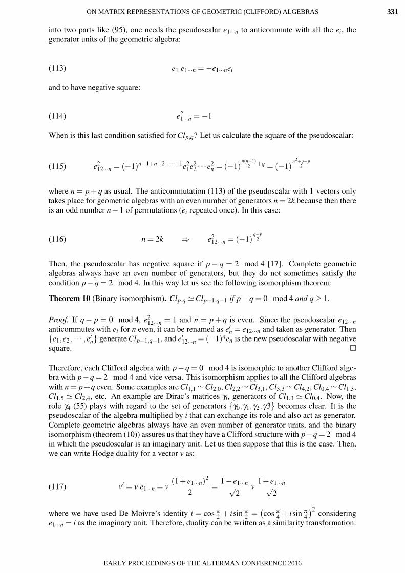
into two parts like (95), one needs the pseudoscalar e1···n to anticommute with all the ei, thegenerator units of the geometric algebra:

(113) e1 e1···n =−e1···nei

and to have negative square:

(114) e21···n =−1

When is this last condition satisfied for Clp,q? Let us calculate the square of the pseudoscalar:

(115) e212···n = (−1)n−1+n−2+···+1e2

1e22 · · ·e2

n = (−1)n(n−1)

2 +q = (−1)n2+q−p

2

where n = p+q as usual. The anticommutation (113) of the pseudoscalar with 1-vectors onlytakes place for geometric algebras with an even number of generators n = 2k because then thereis an odd number n−1 of permutations (ei repeated once). In this case:

(116) n = 2k ⇒ e212···n = (−1)

q−p2

Then, the pseudoscalar has negative square if p− q = 2 mod 4 [17]. Complete geometricalgebras always have an even number of generators, but they do not sometimes satisfy thecondition p−q = 2 mod 4. In this way let us see the following isomorphism theorem:

Theorem 10 (Binary isomorphism). Clp,q Clp+1,q−1 if p−q = 0 mod 4 and q ≥ 1.

Proof. If q− p = 0 mod 4, e212···n = 1 and n = p+ q is even. Since the pseudoscalar e12···n

anticommutes with ei for n even, it can be renamed as e′n = e12···n and taken as generator. Thene1,e2, · · · ,e′n generate Clp+1,q−1, and e′12···n = (−1)qen is the new pseudoscalar with negativesquare.

Therefore, each Clifford algebra with p−q = 0 mod 4 is isomorphic to another Clifford alge-bra with p−q = 2 mod 4 and vice versa. This isomorphism applies to all the Clifford algebraswith n= p+q even. Some examples are Cl1,1 Cl2,0, Cl2,2 Cl3,1, Cl3,3 Cl4,2, Cl0,4 Cl1,3,Cl1,5 Cl2,4, etc. An example are Dirac’s matrices γi, generators of Cl1,3 Cl0,4. Now, therole γ4 (55) plays with regard to the set of generators γ0,γ1,γ2,γ3 becomes clear. It is thepseudoscalar of the algebra multiplied by i that can exchange its role and also act as generator.Complete geometric algebras always have an even number of generator units, and the binaryisomorphism (theorem (10)) assures us that they have a Clifford structure with p−q= 2 mod 4in which the pseudoscalar is an imaginary unit. Let us then suppose that this is the case. Then,we can write Hodge duality for a vector v as:

(117) v′ = v e1···n = v(1+ e1···n)2

2=

1− e1···n√2

v1+ e1···n√

2

where we have used De Moivre’s identity i = cos π2 + isin π

2 =(cos π

4 + isin π4

)2 consideringe1···n = i as the imaginary unit. Therefore, duality can be written as a similarity transformation:



(118) v′ = t−1v t t =1+ e1···n√

2or simply t = 1+ e1···n

for Clifford structures p−q = 2 mod 4, which include all the complete geometric algebras ifa suitable election of generators is taken. This case includes the important space-time algebraCl3,1.Warning. The operator (118) acts exactly as Hodge duality for the grades 1, · · · ,n− 1 but itleaves scalars and pseudoscalars invariant. For instance, we have:

(119) e′1 = e2···n

Then we expect that:

(120) 1′ = (e21)

′ = (e′1)2 = e2···n2 = 1

This is ensured by a similarity transformation. Then it is not right and makes no sense to saythat the dual of scalars are pseudoscalars and vice versa. Notice that if instead of ei you takeas generators of the complete geometric algebra their dual units e1···i−1,i+1,···n, their productgenerates the same pseudoscalar. Then, duality does not change pseudoscalars as commonlyargued in some textbooks, and its right operator is (118).Let us now see whether the three main involutions can be written as similarity transformationsof matrices.

7.5. Grade involution. It consist of changing the direction of 1-vectors. For geometric al-gebras with an even number of generator units, the pseudoscalar anticommutes with vectors,which suffices to state the grade involution operator:

(121) v′ = (e1···n)−1 v e1···n =−v if n = 2k

As usual, the similarity transformation operator applies to all the elements of geometric alge-bra. Then 2-vectors do not change, 3-vector changes the sign and so on. The grade involutionis clearly a direct isometry.

8. INDIRECT ISOMETRIES

Let us recall the definition (5) of indirect isometries. Indirect isometries are the antiautomor-phisms of a geometric algebra, which change the order of the factors when applied to a product.An example of antiautomorphism (and involution) of geometric algebras is reversion.

8.1. Reversion. Reversion R is the transformation that changes the order of the basis vectorsin any given multivector [18]:

(122) R(ei···k) = ek···i

The number of necessary permutations of adjacent vectors in order to reverse the unit e1···k isk(k−1)/2:

(123) e1···k = (−1)k−1+k−2+···+1ek···i = (−1)k(k−1)

2 ek···i



Depending on the value of k mod 4 we have the following cases:

(124) k mod 4 =

0, 1 ⇒ k(k−1)2 even ⇒ R〈e〉k = 〈e〉k

2, 3 ⇒ k(k−1)2 odd ⇒ R〈e〉k =−〈e〉k

where 〈e〉k indicates not only e1···k but any other unit of grade k. Then scalars and 1-vectors donot change the sign, 2-vectors and 3-vectors change the sign and so on.Reversion is an involutory antiautomorphism:

(125) ∀ ui ∈Clp,q R(u1 · · · un) = R(un) · · ·R(u1)

(126) R(R(u1 · · · un)) = u1 · · · un

If ui are vectors then reversion simply changes their order:

(127) (u1 · · · un)′ = un · · ·u1 ∀ ui ∈

⟨Clp,q

⟩1

which is a consequence of (124) owing to the distributive property of the geometric product.Let us see the following theorem about indirect isometries.

Theorem 11 (Inner antiautomorphism). Any indirect isometry of a geometric algebra Clp,qwith n = p+ q even (including complete geometric algebras) is the composition of reversionwith a similarity transformation of matrices.

Proof. Let S be an indirect isometry, R the reversion and T = S R a direct isometry. Then wehave:

(128)S(u v) = S(v)S(u) ⇒ T (u v) = S(R(u v)) = S(R(v)R(u))

= S(R(u))S(R(v)) = T (u)T (v)

On the other hand, S and R are linear and therefore T . In consequence T is an automorphism anda direct isometry. Since every direct isometry T can be written as a similarity transformation ofmatrices for n = p+q even, we finally have:

(129) S(u v) = S(v)S(u) ⇒ S(u) = t−1R(u) t ∀u,v ∈Clp,q p+q = 2k

Let us now review some indirect isometries:

8.2. Clifford conjugation. Clifford conjugation ∼ is the composition of reversion and gradeinvolution. Therefore, Clifford conjugation is an involutory antiautomorphism and an indirectisometry:

(130) u′ = (e1···n)−1R(u) e1···n

Chisholm and Farwell [18] gave how the signs of multivectors change for reversion, gradeinvolution and Clifford conjugation. Their table 27.1.3 can be summarized in the followingtable:



Sign changes of 〈e〉k under main involutions of Clifford algebras Clp,q

0 ≤ k ≤ n = p+q Reversion Grade involution Clifford conjugation

k = 0 mod 4 + + +k = 1 mod 4 + − −k = 2 mod 4 − + −k = 3 mod 4 − − +

TABLE 2. + means that 〈e〉k is preserved, and − means that its sign is changedunder the involution: 〈e〉′k =−〈e〉k.

8.3. Transposition or Hermitian conjugation. Transposition (usually denoted with T ) is thetransformation consisting of the transposition of the real matrix representation of every elementin a geometric algebra. Transposition is an antiautomorphism:

(131) (u v)T = vT uT (λu+µv)T = λuT +µvT ∀u,v ∈Clp,q λ ,µ ∈ R

Let us see that complex numbers become conjugate under transposition:

(132) (a+b i)T =

(a b−b a

)T

=

(a −bb a

)= a−b i = (a+b i)∗

The Hermitian conjugate (usually represented with †) of a matrix with complex entries is de-fined as the transpose matrix with complex conjugate entries. If a complex matrix is expandedby means of direct product with the real representation of complex numbers given above, theHermitian conjugate corresponds to the transposition of the expanded real matrix. Let us see,how units change under transposition.

Theorem 12 (Symmetry of unit matrices). The real representations of units with positive ornegative square are respectively symmetric or skew-symmetric matrices.

Proof. Let u be a unit having positive square, and let v be an eigenvector (column matrix) of uwith eigenvalue λ . Then

(133) u2 = I, u v = λ v ⇒ u2 v = v = λ 2v ⇒ λ 2 = 1

where I is the identity matrix. Multiplying u v by the transposed matrices we have:

(134) vT uT u v = vT λ 2v = vT v ⇒ uT u = I

But u is a unit such that u2 = I. Then:

(135) uT u = I = u2 ⇒ uT = u2u−1 = u

That is, the real representation of a unit having positive square is a symmetric matrix:



(136) u2 = I ⇒ uT = u

Let us now suppose that the unit u has negative square, and let v be an eigenvector (columnmatrix) of u with eigenvalue λ :

(137) u2 =−I, u v = λ v ⇒ u2 v =−v = λ 2v ⇒ λ 2 =−1

Since the eigenvalues are imaginary, there are invariant subspaces for v with dimension 2, andλ must be treated as a matrix:

(138) λ =±i =±(

0 1−1 0

)

Multiplying u v by the transposed matrices we have:

(139) vT uT u v = vT λ T λv = vT v ⇒ uT u = I

But u is a unit such that u2 =−I. Then:

(140) uT u = I =−u2 ⇒ uT =−u2u−1 =−u

That is, the real representation of units with negative square are skew-symmetric matrices:

(141) u2 =−I ⇒ uT =−u

In fact, Hermitian conjugation has been already defined from its action under the units of thegeometric algebra[18]:

(142) e†i···k = ei···k ⇐⇒ e2

i···k = Ie†

i···k =−ei···k ⇐⇒ e2i···k =−I

The operator of Hermitian conjugation must discriminate units with positive square from unitswith negative square, and it seems that in Clp,q the unit e1···p could be the suitable operator. Letus see how it is exchanged with vector units:

(143)

p odd ⇒

eie1···p = e1···pei if i ≤ peie1···p =−e1···pei if i > p

p even ⇒

eie1···p =−e1···pei if i ≤ peie1···p = e1···pei if i > p

where 1 ≤ i ≤ n = p+q. On the other hand, we also have:



(144)

q odd ⇒

eiep+1···p+q =−ep+1···p+qei if i ≤ peiep+1···p+q = ep+1···p+qei if i > p

q even ⇒

eiep+1···p+q = ep+1···p+qei if i ≤ peiep+1···p+q =−ep+1···p+qei if i > p

The suitable anticommutation with unit vectors having negative square (Hermitian conjugation)is only possible for p odd or q even. All geometric algebras admit one of both possibilities.If p is even and q is odd, then the isomorphism Clp,q Clq+1,p−1 (valid for all geometricalgebras[6]) changes the parity of p and q. Then, the general operator of Hermitian conjugationis:

(145) ∀v ∈Clp,q

p odd v† =(e1···p

)−1 R(v)e1···p

q even v† =(ep+1···p+q

)−1 R(v)ep+1···p+q

Of course, reversion must also be applied since Hermitian conjugation is the same as trans-position of real matrices, which is an antiautomorphism. In the important case of space-timegeometric algebra Cl3,1, Hermitian conjugation is obtained through the operator e123.

(146) v† = (e123)−1 R(v)e123 ∀v ∈Cl3,1

For instance:

(147) e†0 = (e123)

−1 e0e123 =−(e123)−1 e123e0 =−e0

(148) e†123 = (e123)

−1 R(e123)e123 = (e123)−1 e321e123 = (e123)

−1 =−e123

since e2123 =−1.

From the Hermitian conjugation (145), we can isolate reversion to get a useful formula forreversion:

(149) ∀v ∈Clp,q

p odd R(v) = e1···p v† (e1···p)−1

q even R(v) = ep+1···p+q v† (ep+1···p+q)−1

The equalities (124) yield a fast algorithm for computing reversion with matrix representation.If the matrices are real, Hermitian conjugation consists of the very easy algorithm of taking thetranspose matrix. Then, after multiplication by the matrix representation of the product of theunits with positive or negative square depending on the case, we have reversed the matrix veryfastly. For instance, in Cl3,1 M4×4, using the Majorana representation (61) we have for everyelement represented by a matrix A:

(150) R(A) = e123 AT (e123)−1 =

0 0 1 00 0 0 1−1 0 0 00 −1 0 0

AT

0 0 −1 00 0 0 −11 0 0 00 1 0 0



without resolving A in multivectors.

Since every square matrix can be resolved into an addition of a symmetric matrix and a skew-symmetric matrix in a unique way, the linear space of square matrices of order m is directsum of the linear space of skew-symmetric matrices of the same order, which has dimensionm(m− 1)/2, and the linear space of symmetric matrices, which has dimension m(m+ 1)/2.Therefore, the total number w of units with positive and negative square in the basis of a com-plete geometric algebra Clp,q is:

(151) w+ = 2n2−1(2

n2 +1) w− = 2

n2−1(2

n2 −1) n = p+q

because m = 2n2 . For instance Cl3,1 M4×4(R) has n = 4, w+ = 10 and w− = 6.

9. CONCLUSIONS

The norm of every element v of a geometric algebra is defined as the kth-root of the absolutevalue of the determinant of its real square matrix representation Mk×k(v), and isometries aredefined as those transformations that commute with the power of every element of the algebraT (vn) = [T (v)]n. Therefore isometries preserve the characteristic polynomial of the matrix rep-resentation of every element. Then, direct isometries of a geometric algebra are defined as itsautomorphisms, while indirect isometries are defined as its antiautomorphisms. For the geo-metric algebras Clp,q with n = p+q even, which are central simple algebras, direct isometriescan be written as similarity transformations of matrices T (u) = t−1u t, while indirect isometriescan be written as the composition of reversion R with similarity transformations of matrices.In this way, rotations, reflections, axial symmetries, duality, Clifford conjugation, transpositionand Hermitian conjugation are reviewed and written in canonical form (in the two ways indi-cated above). Canonical forms T (u) = t−1u t or S(u) = t−1R(u) t for isometries can be appliedto every element of the geometric algebra, homogeneous or heterogeneous in grade, which hasnot only theoretical importance but also practical usefulness since it simplifies algorithms forprogrammers.

REFERENCES

[1] D. Hestenes, Space-Time Algebra, Birkhauser, 2015.[2] A. D. Aleksandrov, A. N. Kolmogorov, M. A. Laurentiev, La matematica: su contenido, metodos y signifi-

cado, v. III, p. 392. Alianza Editorial, 5th ed., 1982.[3] W. R. Hamilton, Elements of Quaternions (1869). Ed. by Charles Jasper Joly, 3rd edition, Chelsea publishing

company (N. Y., 1969).[4] J. B. Kuipers, Quaternions and Rotation Sequences, Princeton Univ. Press, p. 130, 1999.[5] R. Delanghe, F. Sommen, V. Soucek, Clifford Algebras and Spinor-Valued Functions, Kluwer (Dordrecht,

1992) p. 81.[6] P. Lounesto, Clifford Algebras and Spinors, Cambridge Univ. Press (Cambridge, 1997) pp. 215-217.[7] J. W. Gibbs. On the Role of Quaternions in the Algebra of Vectors. Nature, XLIII: 511-513, April 2, 1891.

Ibidem 155-160.[8] P.A.M. Dirac, “The Quantum Theory of the Electron”, Proc. Roy. Soc. 117 (1928) pp. 610-624.[9] E. Majorana, “Teoria simetrica dell’electrone e del positrone”, La vita e l’opera di Ettore Majorana, Ac-

cademia Nazionale dei Lincei (Roma, 1966), pp 67-79. A facsimile edition has been published recently byBardi Editore.

[10] J. Snygg, Clifford Algebra. A Computational Tool for Physicists, Oxford Univ. Press (1997), p. 11.[11] C. D. H. Chisholm, Group Theoretical Techniques in Quantum Mechanics, Academic Press (London, 1976)

p. 167.[12] E. Cartan, “Nombres complexes”, Encyclop. Sc. Math. ed francaise, 15 (1908) pp. 329-468.[13] R. Gonzalez Calvet, El algebra geometrica del espacio y tiempo, p.12. Available at

http://www.xtec.cat/∼rgonzal1/espacio.htm .



[14] L. Landau, E. Lifshitz, Curso abreviado de Fısica teorica vol. I, Mecanica y Electrodinamica, Mir (Moscow,1971) p. 172.

[15] R. Ablamowicz, B. Fauser,“On the transposition anti-involution in real Clifford algebras II: Stabilizergroups of primitive idempotents” Linear and Multilinear Algebra 59 (2011) 1359-1381.

[16] E. Noether “Nichtkommutative Algebren”, Math. Zs. 37 (1933) 514-541. Reproduced in Emmy Noether,Gesammelte Abhandlungen, Collected Papers, Springer (Berlin, 1983) 642.

[17] R. Gonzalez Calvet, “New foundations for geometric algebra”, Clifford Analysis, Clifford Algebras andtheir Applications 2 (2013) pp. 193-211.

[18] J. S. R. Chisholm, R. S. Farwell, “Properties of Clifford Algebras for Fundamental Particles”, Clifford(Geometric) Algebras, ed. by W. E. Baylis, Birkhauser (1996), pp. 365-388.



BINOCULAR COMPUTER VISION BASED ON CONFORMAL GEOMETRICALGEBRA

J. Hrdina a and A. Navrat a

a Institute of MathematicsNETMe Centre, Division of Mechatronics

Faculty of Mechanical EngineeringBrno University of Technology.


ABSTRACT. We solve a generalized binocular vision problem by means of conformal geomet-ric algebra. We consider two cameras whose position is determined by an arbitrary Euclideantransformation which can depend on an arbitrary number of parameters. We represent thesetransformations by algebra elements which allows us to derive general equations of 3D objectreconstruction from two camera projection planes by formal manipulation in conformal geomet-ric algebra. Such equation can be solved w.r.t. either motor or projection unknown parameters,the others can be determined consequently. We present two specific examples, show the explicitform of two particular motors and solve the appropriate equations completely.

1. INTRODUCTION

Binocular vision problem can be understood as two particular objectives, i.e. 3D objectreconstruction from the data obtained by a pair of cameras and the converse decomposition ofa 3D object into two projection planes. Our task is to define the camera position transformationto achieve the prescribed shape of an object in question whose position is given as part of theinput data. Typically, this is solved to centre the observed object on one camera. Furthermore,we assume that the cameras are in arbitrary mutual position whose parameters are the onlydata needed. In classical literature, e.g. [5, 1], the coordinate system is attached to one ofthe cameras which will be referred to as the first one. In our case, we choose the coordinatesystem connected to the base of the camera stand to simplify the correspondence of the rotationaxes. We consider both cameras to be the pin–hole model and introduce the description ofeach of them as a pair of algebra elements, more precisely as a point F (focus) and a pointpair K = P∧Q from the camera projection plane such that the lines F ∧P∧ e∞ and K ∧ e∞ areorthogonal.

In this setting, the problem is solved by symbolic computations with conformal geomet-ric algebra (CGA) objects in general, but we discuss the projective geometric algebra (PGA)setting simultaneously. Indeed, the last Section shows one of possible directions that we intendto explore in the future, particularly the human vision where PGA is not sufficient tool. Anotherdirection to be considered is e.g. the image analysis from the omnidirectional camera.

The reason to use the GA (CGA) structures to solve such topics lies in the fact that theproperties are invariant of the particular mechanism. In paricular, we derive formulas (3) and(4) which hold in general for any system. In Section 5 we show on two elementary examples theapplication of our computations onto two particular mechanisms and we present the numericresults for several specific settings. In the sense of an object oriented approach, we divide thebinocular vision problem into three parts. The most abstract one contains the elaboration withthe GA elements by means of standard operations and exploits their natural properties as theOPNS and IPNS representation of the Euclidean object. Our aim is to achieve a mechanismindependent geometric solution. Afterwards, we choose a particular GA (despite the fact that

339


in this text we assume to work within CGA and use several arguments valid for CGA only,from the remarks in the text it is obvious that e.g. in the case of a pin–hole camera the choiceof CGA is not completely necessary). Finally, we introduce the equations of the particularmechanism which follows from the forward kinematic chain. Thus in general, the motorstransforming the camera position from the initial ideal state to the actual one are obtained.Note that the computations are performed in Maple, package CLIFFORD [7], and the finalset of equations, whose form does not demand deeper knowledge of CGA, can be used inengineering applications.

2. CONFORMAL GEOMETRIC ALGEBRA – CGA

We recall some elementary facts about CGA and specify our particular setting. Notethat the properties and definitions of conformal geometric algebras can be found in e.g. [2,5]. Classically, for modelling a 3D robot, the CGA is the Clifford algebra C l(4,1) and anembedding

c : R3 →K4 ⊂ R

4,1

of the 3D Euclidean space is considered, where K4 is a null cone in the Minkowski space

R4,1. We describe the embedding explicitly in a suitably chosen basis which is denoted by

e0,e1,e2,e3,e∞ ∈ R4,1 usually. Namely, the basis is chosen such that the appropriate quadratic

form is

B =

0 0 −1

0 13×3 0−1 0 0

,

where 13×3 is an identity 3×3 matrix. Consequently, the embedding is of the form

c(x) = x+12

x2e∞ + e0.

Note that e0 and e∞ play the role of the origin and the infinity, respectively. Note also that x2 isa scalar which is equal to ‖x‖2, the square of usual Euclidean norm. We recall that the algebraoperation is called the geometric (Clifford) product and two further elementary operations onCGA are derived; the inner product (left contraction) and outer (wedge) product. We recall justthe basic properties used within the following text. On R

4,1, the inner product and outer productcorrespond to the symmetric and antisymmetric part of the geometric product, respectively.Generally, the wedge product of two basis blades Ek and El of grades k and l, respectively, isdefined as

Ek ∧El := 〈EkEl〉k+l

and the left contraction is defined as

Ek ·El := 〈EkEl〉l−k if l ≥ k and 0 otherwise,

where 〈〉k is the grade projection into grade k. Consequently, the inverse mapping c−1 : K4 →R

3 is defined by

c−1(x) = P⊥e∞∧e0

(x

−x · e∞

)= x+

x · (e∞ ∧ e0)−1

x · e∞(e∞ ∧ e0),

where P⊥ denotes the orthogonal complement to the projection onto e∞ ∧e0. The embedding chas the fundamental property that the inner product of two conformal points is, up to the factor

BINOCULAR COMPUTER VISION BASED ON CONFORMAL GEOMETRIC ALGEBRA340


−1/2, the square of the Euclidean distance. Indeed,

c(x) · c(y) =(

x+ 12x2e∞ + e0

)·(

y+ 12y2e∞ + e0

)

=⟨

xy+ 12(y

2x− x2y)e∞ +(x− y)e0 +12x2e∞e0 +

12y2e0e∞

⟩0

= xy− 12x2 − 1

2y2 =−12(x− y)2 =−1

2‖x− y‖2.

Thus the embedding c, together with the inner product, gives a linearization of a squared dis-tance. As a consequence, the round objects which are given by quadratic expressions (spheres)are represented by linear objects and the Euclidean motions are represented by orthogonaltransformations.

Algebraically, we consider the geometric algebra on R4,1, i.e. the algebra denoted as G4,1

which is the Clifford algebra C l(4,1). In terms of the basis e0,e1,e2,e3,e∞ of R4,1, a basis ofG4,1 is given by Grassmann monomials (blades) as displayed in tabular 1.

scalars 1vectors e1, e2, e3, e0, e∞2–blades e1 ∧ e2, e1 ∧ e3, e1 ∧ e0, e1 ∧ e∞, e2 ∧ e3,

e2 ∧ e0, e2 ∧ e∞, e3 ∧ e0, e3 ∧ e∞,e0 ∧ e∞3–blades e1 ∧ e2 ∧ e3, e1 ∧ e2 ∧ e0, e1 ∧ e2 ∧ e∞, e1 ∧ e3 ∧ e0,

e1 ∧ e3 ∧ e∞, e1 ∧ e0 ∧ e∞, e2 ∧ e3 ∧ e0, e2 ∧ e3 ∧ e∞,e2 ∧ e0 ∧ e∞, e3 ∧ e0 ∧ e∞

4–blades e1 ∧ e2 ∧ e3 ∧ e0, e1 ∧ e2 ∧ e3 ∧ e∞, e1 ∧ e2 ∧ e0 ∧ e∞,e1 ∧ e3 ∧ e0 ∧ e∞, e2 ∧ e3 ∧ e0 ∧ e∞

pseudoscalar I = e1 ∧ e2 ∧ e3 ∧ e0 ∧ e∞TABLE 1. Wedge basis of C l(4,1)

The Euclidean objects which can be represented by elements in this algebra are spheresof any dimension in particular, i.e. point pairs, circles, spheres, points (spheres of zero radius),linear objects of any dimension, i.e. flat points, lines, planes, and also Euclidean directionaland tangential elements. They are represented in the following way. Let S ⊆ R

3 is one of theEuclidean elements listed above. Then it is viewed as an element S ∈G4,1 such that

x ∈ S ⇔ c(x)∧S = 0.

Note that this is so–called outer product representation (OPNS). Dually, i.e. in IPNS represen-tation, S is represented by an element S∗ and the condition reads

x ∈ S ⇔ c(x) ·S∗ = 0.

Note that on the algebra level the duality is obtained by dividing an algebra element S by thepseudoscalar I, i.e. S∗ = S/I.

In the OPNS representation, the outer product ∧ indicates the construction of a geometricobject with the help of points Pi that lie on it. A point pair (0D sphere) is defined by two pointsP1 ∧P2. A circle (1D sphere) is defined by three points P1 ∧P2 ∧P3 or a point pair and a point.Finally, a sphere (2D sphere) is defined by four points P1 ∧P2 ∧P3 ∧P4 or two point pairs, etc.A plane and line can also be defined by points that lie on it and by the point at infinity, i.e. aline is represented by P1 ∧P2 ∧ e∞ and a plane by P1 ∧P2 ∧P3 ∧ e∞. In IPNS, a sphere can berepresented by its center P and its radius r as P− 1

2r2e∞. A plane is defined as n+de∞, wheren is the normal vector of the plane and d is the distance to the origin.

BINOCULAR COMPUTER VISION BASED ON CONFORMAL GEOMETRIC ALGEBRA 341


In this sense, the wedge product is a constructive operator, i.e. A∧B is an object spannedby A and B etc. The duality operator allows for a definition of the dual to wedge product, socalled meet,

A∨B = (A∗ ∧B∗)∗.Geometrically, this gives a CGA representative of the intersection of objects A and B.

The next advantage of CGA is that the Euclidean motions are also represented by certainalgebra elements. Namely, an Euclidean transformation of an element S is in CGA realized byconjugation with a unique orthogonal invertible element T ∈G4,1, i.e.

S → T ST−1.

Note that the inverse T−1 can be replaced by reverse T since for orthogonal transformationsT T = 1 , [5]. For instance, the translation in the direction t = t1e1 + t2e2 + t3e3 is realized bythe multivector (translator)

T = 1− 12

te∞

and the rotation around the origin and the normalized axis L = (L1,L2,L3) by an angle φ isrealized by the multivector (rotor)

R = e−12 Lφ = cos

φ2−Lsin

φ2,

where L = L1(e2∧e3)+L2(e3∧e1)+L3(e1∧e2). The rotation around a general point and axisis then a composition T RT of the translation to the origin, rotation R and reverse translation. Ageneral composition of a translator with a rotor is called a motor.

Remark 2.1. For some aplications it is sufficient to consider an embedding in a 4D projec-tive space only. To generate three dimensional projective geometric algebra (PGA), Euclideanvectors are embedded in an four dimensional affine space:

p(x) = xe1 + ye2 + ze3 + e4

where the ei are the canonical basis of R4. If a ∈ R3, then the corresponding homogenized

vector p(a) is denoted as A and given vector A ∈G4, the corresponding Euclidean vector is

a =A

A · e4− e4.

Using the concept OPNS the bivector A∧B represents the line trough a and b (after homogeni-sation), where A = p(a),B = p(b) are the points. Finally, OPNS of the outer product of threehomogeneous vectors in G3 represents a plane. Note that this PGA approach is implicitlycontained in the CGA approach.

3. CAMERA POSITION

First of all, we need to describe efectively a position of a camera in space. We representthe camera by two CGA elements

• conformal point F representing the camera center (focus),• point pair P∧Q defining the camera image plane π ,

as illustrated in figure 1. We can obtain the classical camera descriptions by straightforwardcomputations as

• focal distance f =−2√

F ·P,• camera direction (F −P)∧ e∞,• camera plane π = P∧Q∧ (F ∧P∧ e∞)

∗.



FIGURE 1. Description of camera position

Note that the line P∧Q∧ e∞ has to be always orthogonal to line F ∧P∧ e∞, i.e.

(F ∧P∧ e∞) · (P∧Q∧ e∞) = 0.

Given an initial position F0,P0,Q0, the actual position in the space is obtained by an Euclideantransformation which in CGA is given by a conjugation with a motor M (see figure 1 again).The advantage of CGA is that we can transform the whole geometric objects, i.e. any geometricentity constructed from F,P,Q. For instance, the actual position of the camera center is

(1) F = MF0M,

and the actual position of the image plane is given by

(2) π = Mπ0M.

In the same way, one can obtain also the actual camera direction M((F0 −P0)∧ e∞)M etc. Fora concrete application one only needs to specify the initial position and the motor M.

Remark 3.1. In PGA, the camera position is also represented by two objects; the projectivepoint F representing the camera center and line P∧Q which lies in camera plane such that theline P∧Q is orthogonal to line F ∧P, i.e. (F ∧P) · (P∧Q) = 0. Similarly to CGA, the cameraimage plane is obtained as π = P∧Q∧ (F ∧P)∗.

4. POSE ESTIMATION

Let us have two cameras in a general position, given by two arbitrary motors M1, M2,and a line symmetry L which projects to conjugate lines L1, L2 in the two camera image planesπ1, π2 (see figure 2). We show how simple is to compute the images of L or to reconstruct Lfrom its images by CGA approach. Indeed, given a line L in 3D, its image on a camera planeis given as the intersection of these plane with a plane spanned by L and the correspondingcamera focus. In terms of the wedge product and the meet we thus have

(3) Lk = (L∧Fk)∨πk, k = 1,2,

where the current positions Fk and πk are computed from their initial position by (1) and (2),respectively, with M being either M1 or M2. Concerning the inverse problem, the real line isreconstructed from the given images as the intersection of the plane spanned by L1 and F1 withthe plane spanned by L2 and F2. Thus its representative in CGA reads

(4) L = (F1 ∧L1)∨ (F2 ∧L2).



FIGURE 2. A line symmetry projected to two cameras

Let us emphasize that formulas (3), (4) are valid for cameras in general positions based onarbitrary motors M1 and M2 and that the computation above are valid for conformal geometricalgebra and also for the projective geometric algebra.

Note that the conjugate lines L1 and L2 are considered as lines in 3D space. For applica-tions we would rather need to express them in the 2D image coordinates. Therefore, we definemaps ιk : R2 →R

3 which transform the xy–plane into πk, k = 1,2. Then a formula for Lk in theplanar image coordinates is given by ι−1

k (Lk). Hence

L2Dk := ι−1

k (Lk) = δke1 ∧ e2 ∧ e∞ + cos(αk)e1 ∧ e∞ ∧ e0 + sin(αk)e2 ∧ e∞ ∧ e0,

for a suitable planar Pluckner coordinates based on δk and αk. These can be extracted from Lkas follows

Lk = (e0 ∧ e∞) ·L2Dk ,

(δk)∗ = (L2D

k −Lk ∧ e0 ∧ e∞)∧ e3 ∧ e0,

whereLk ≡ cos(αk)e1 + sin(αk)e2. Indeed, compute (e0 ∧ e∞) ·L2Dk as

〈(e0 ∧ e∞) · ι−1k (Lk)〉3−2

= 〈δk(e0 ∧ e∞)(e1 ∧ e2 ∧ e∞)+ cos(αk)(e0 ∧ e∞)(e1 ∧ e∞ ∧ e0)+ sin(αk)(e0 ∧ e∞)(e2 ∧ e∞ ∧ e0)〉1

= 〈δk(−1− e0e∞)(e1e2e∞)+ cos(αk)(−1− e0e∞)(e1(1+ e∞e0))+ sin(αk)(−1− e0e∞)(e2(1+ e∞e0))〉1

= 〈−δk(e1e2e∞)+ cos(αk)(−e1(1+ e∞e0)− e0e∞e1)+ sin(αk)(−e2(1+ e∞e0)− e0e∞e2)〉1

= 〈−δk(e1e2e∞)+ cos(αk)(−e1 − e1e∞e0 − e0e∞e1)+ sin(αk)(−e2 − e2e∞e0 − e0e∞e2)〉1

=−cos(αk)e1 − sin(αk)e2.

In the very similar way compute (L2Dk −Lk ∧ e0 ∧ e∞) as

δke1 ∧ e2 ∧ e∞ + cos(αk)e1 ∧ e∞ ∧ e0 + sin(αk)e2 ∧ e∞ ∧ e0 +(cos(αk)e1 + sin(αk)e2)∧ e0 ∧ e∞

= δke1 ∧ e2 ∧ e∞

and finally,

(L2Dk −Lk ∧ e0 ∧ e∞)∧ e3 ∧ e0 = δke1 ∧ e2 ∧ e∞ ∧ e3 ∧ e0 = (δk)

∗.

Let us remark that, in the inverse problem, we do not need to read off the Plucknercoordinates directly. If we read off two points [x1

k ,y1k ], [x

2k ,y

2k ] of the line Lk instead, then we get

ι−1k (Lk) = (x1

ky2k − x2

ky1k)e1 ∧ e2 ∧ e∞ +(x2

k − x1k)e1 ∧ e∞ ∧ e0

+(y2k − y1

k)e2 ∧ e∞ ∧ e0.



Remark 4.1. In PGA, the geometric elements F1,F2,L1,L2,L,π1,π2 are represented differently(in a 4D space) but the fundamental formulae (3) and (4) have exactly the same form.

5. MODELS AND THE PROBLEM

We will demonstrate our apparatus on two models; each of them constitutes of two pin-hole cameras but their relative position and freedome is different. The problem is to adapt thegiven system by changing free parameters (angles of rotations) such that the image of a givenline in one camera or in both cameras (if possible) is in a specific position. Concretly, in theexamples below we want the image in one of the camera to be centered exactly to the x–axis ofthe image coordinates. This problem in general is solved completely by formulas (3) and (4).An explicit solution is solved by the following algorithm based on these formulas. We considerthat the configuration of a given system depends on a set of parameters φ = (φ1,φ2, · · ·) andour aim is to find φ such that the image of a line in the k–th camera coincides with a givenreference line Lre f

k (x–axis in the examples below). Note that the algorithm has two parts. Inthe first one, we reconstruct the world line L from its images captured by the camera system ina configuration φ0. The second part computes images of L in a general configuration φ.

• specify the system by specifying two motors M1,M2 and the map ιk and their depen-dance on parameters φ,

• an input: two 2D images L2D1 ,L2D

2 of a real line L captured on cameras in a positionsdescribed by parameters φ0,

• compute Lk(φ0) = ιk(L2D

k ) for k = 1,2,• compute positions of camera centers for k = 1,2 according to (1)

Fk(φ0) = Mk(φ

0)F0Mk(φ0),

• compute the real line L according to (4)

L = (F1(φ0)∧L1(φ

0))∨ (F2(φ0)∧L2(φ

0))

• compute camera centers and image planes in a position φ according to (1) and (2)

Fk(φ) = Mk(φ)F0Mk(φ),

πk(φ) = Mk(φ)π0Mk(φ),

• compute its images in cameras in a position φ according to (3)

Lk(φ) = (L∧Fk(φ))∨πk(φ),

• solve equation ι−1k (Lk(φ)) = Lre f

k for φ.

For both models we consider that the camera initial position is placed in the inertial coordinateframe such that

F0 = c(0,0,0) = e0,

P0 = c(0,0, f ) = f e3 +12

f 2e∞ + e0,

Q0 = c(0,1, f ) = e2 + f e3 +12( f 2 +1)e∞ + e0.

Consequently, the initial camera axis F0 ∧P0 ∧ e∞ = f e3 ∧ e∞ ∧ e0 is the z–axis and the initialimage plane π0 = P0 ∧Q0 ∧ (F0 ∧P0 ∧ e∞)

∗ is given by

π0 =−12

f 2e1 ∧ e2 ∧ e3 ∧ e∞ +12

f e1 ∧ e2 ∧ e∞ ∧ e0.



The map ιk : R2 → R3 maps xy–plane to π0 (the translation about the focal distance f in the

z–direction) and then to πk (transformation Mk) and thus is given by conjugation by the motorMkexp(−1/2 f e3 ∧ e∞), k = 1,2, i.e.

ιk(L2Dk ) = Mk(1− f

2e3 ∧ e∞)L2D

k (1+f2

e3 ∧ e∞)Mk.

Since it is an orthogonal transformation in CGA, its inverse is given simply by a conjugationby the reversed motor. Now we have all what we need to solve the problem in CGA, except thespecification of M1 and M2.

5.1. First model. Let us consider a system of two cameras attached to one rotational axissuch that the first of them can rotate also around a perpendicular axis. A precise scheme withan attached coordinate frame is displayed in Figure 3. The formulae for the motors can be read

FIGURE 3. Scheme of the first model

off the figure directly. Namely, we have

M1 = R2R1T1,

M2 = R1,

where the translation T1 and the rotations R1, R2 are given by

T1 = 1− 12

l1e2 ∧ e∞,

R1 = cos(φ1

2)+ sin(

φ1

2)(e3 ∧ e1),

R2 = cos(φ2

2)+ sin(

φ2

2)2

and where the axis 2 of the second rotation is

2 = R1T1(e2 ∧ e3)T1R1.

Thus the appropriate motors are determined and thus a solution can be found accord-ing to the algorithm given above. In this particular example, it is possible to find a com-plete solution in symbolic form using CLIFFORD [7]. Namely, given Pluckner coordinates



(m1,m2,m3,d1,d2,d3) of the world line L, its images in cameras are

L1 =(

m2 cosφ2 − (m1 − l1d3)sinφ1 sinφ2 +(m3 + l1d1)cosφ1 sinφ2

)e1

+((m1 − l1d3)cosφ1 +(m3 + l1d1)sinφ1

)e2

δ1 = f (m1 − l1d3)sinφ1 cosφ2 − f (m3 + l1d1)cosφ1 cosφ2

L2 = m2e1 +(m1 cosφ1 +m3 cosφ1)e2

δ2 = f m1 sinφ1 − f m3 cosφ1

In the opposite way, given Pluckner coordinates (x1,y1,δ1) (x2,y2,δ2) of L1 and L2, respec-tively, the real line L is reconstructed as

m1 = l1x2y1 f 2 sinφ1 cosφ2 − l1x2δ2 f cosφ1 cosφ2 + l1y1δ1 f sinφ1 sinφ2 − l1δ1δ2 cosφ1 sinφ2,

m2 = l1x1x2 f 2 cosφ2 + l1x1δ1 f sinφ2,

m3 = l1x2y1 f 2 cosφ1 cosφ2 + l1x2δ2 f sinφ1 cosφ2 + l1y1δ1 f cosφ1 sinφ2 + l1δ1δ2 sinφ1 sinφ2,

d1 =−y2δ1 f sinφ1 sinφ2 + x2y1 f 2 sinφ1 cosφ2,

− (δ1δ2 + x2y1 f 2)cosφ1 sinφ2 +(x1δ1 f − x2δ2 f )cosφ1 cosφ2,

d2 =−y2δ2 f − x2y1 f 2 sinφ2 + y1δ1 f cosφ2,

d3 = (δ1δ2 + x1x2)sinφ1 sinφ2 +(x1δ1 f − x2δ2 f )sinφ1 cosφ2,

− y1δ1 f cosφ1 sinφ2 − x2y1 f 2 cosφ1 cosφ2.

Now we can solve our main equation

L2Dk (φ) = Lre f

k

for φ explicitly. To present a set of results we choose the kinematic parameters 1 = 1 and f =0.045. Furthermore, we assume that the initial camera positions are determined by the anglesφ 0

1 = 0 and φ 02 = −π

8 . If the Pluckner coordinates coincide within this setting we concludethat the visualized line is placed in front of the system. We set the angle to be π

10 , π20 and π

100 ,respectively, and the appropriate distance to be 0.1 and 0.01. The numeric results are shown incolumns three to four of Table 2.

The image within camera number one can be placed into Pluckner plane coordinates(1,0,0) by a combination of both rotation changes. The larger the object distance, the rotationchanges become more minor. Clearly, the data in the above table correspond with the fact thatif d1,2 is decreased the visualized object is becoming more remote.

5.2. Second model. The second model (see figure 4) is also based on two revolute joints,represented by angles rotations R1,R2 but the cameras do not lie one on one axis. In this case,the system can be described by the following set of motors.

M1 = R1T1,

M2 = R2R1T2,



FIGURE 4. Scheme of the second model

where the translations T1,T2 and the rotations R1, R2 are given by

T1 = 1− 12

l1e2 ∧ e∞,

T2 = 1− 12

l2e1 ∧ e∞,

R1 = cos(φ1

2)+ sin(

φ1

2)(e3 ∧ e1),

R2 = cos(φ2

2)+ sin(

φ2

2)2

and where the axis 2 of the second rotation is

2 = R1(e2 ∧ e3)R1.

φ1,2 d1,2 First model: r1 r2 Second model: r1 r2

π/10 0.1 -3.01 1.56 0.14 4.310.01 -2.64 0.68 0.95 0.38

π/20 0.1 -3.08 1.55 0.07 1.150.01 -2.88 0.63 0.61 0.27

π/100 0.1 -3.13 1.54 0.01 1.150.01 -3.09 0.61 0.14 0.22

TABLE 2. The results where the image of a line in the camera coincides with x–axis

Finally, we present an example given by the kinematics setting 1 = 1, 2 = 0.5 andf = 0.045. The initial configuration is given by φ 0

1 = φ 02 = 0 and the Pluckner coordinates are

the same as in the first model. The numeric results are shown in columns five to six of Table 2.again, the data in the above table correspond with the fact that if d1,2 is decreased the visualizedobject is becoming more remote.

6. HUMAN–LIKE VISION

The models described above can be solved alternatively in PGA since all objects whichoccured were flat, i.e. points, lines and planes, as remarked in 3.1 and 4.1. However, theCGA approach allows for generalizations like human–like vision. By this expression, we meana binocular vision as above but with cameras which do not project on plane but rather on asphere. Thus it is similar to human vision but the relative position of “eyes” can vary and maydepend on several parameters. For instance, the “eyes” can rotate as in the models above. In



CGA, sphere is in principle the same as plane and thus we can use the theory from sections 3,4 and also the algorithm from section 5 with minor changes. Instead of a camera plane π , wehave a camera sphere σ but the transformation is the same as in (2), i.e.

σ = Mσ0M.

The role of F is the same and P defines the direction of an “eye”. Instead of Q one needs moredata to recover the whole image sphere σ . The basic formulas (3) and (4) are also still valid butas images of L we get conjugate circles c1,c2 instead of conjugate lines L1,L2, i.e.

ck = (L∧Fk)∨σk, k = 1,2,

L = (F1 ∧ c1)∨ (F2 ∧ c2).

Note that the images c1,c2, even in their initial position, are 3D objects. A possibility howto get an equivalent 2D information is to take their stereographic projections which is easy inCGA. Using CGA one can also easily recover classical notions as the point of fixation or thehoropter. Of course, the fixation does not need to exist in our general setting. But if it exists, itis obviously given by

Fix = (F1 ∧P1 ∧ e∞)∨ (F2 ∧P2 ∧ e∞)

and the horopter circle readsHor = F1 ∧F2 ∧Fix.

7. CONCLUSION

The motivation for this paper is given by a specific engineering application of binocularvision. More precisely, we consider two cameras attached to a mechanic manipulator on differ-ent axes. The whole construction provides several degrees of freedom. The initial setting readsthe position of both cameras and the reference line projection of the observed object. The goalis to identify the reference line and centre it on an arbitrary camera consequently. Note thatwithout the reference line exact 3D position it is not possible to solve the problem, althoughthis was not part of the setting.

We solved this problem for arbitrary manipulator kinematics by means of CGA geo-metric objects and transformations. In Section 5 we introduced the algorithm for a particularkinematics choice and derived the explicit equation ι−1

k (Lk(φ)) = Lre fk the solution of which is

the desired configuration. We solved the problem for two specific configurations including thepresentation of several outputs. Final equations of the first example (Section 5.1) are presentedin the form without the CGA symbolic which we find suitable for applications. Conformalalgebra thus provides an effective system description. Its object oriented nature then allows tosolve several problems simultaneously. The last step demands to solve the system of non linearequations. This should be done in special software that needs the classical form of equations.Note that even the system transformation into the explicit form is realized by CGA elementsmanipulation.

Within the process we needed to describe the inner configuration of a pin–hole camerawhich was done in Section 3. Furthermore, some unknown identities transforming the CGAline description into the Pluckner coordinates were introduced, see Section 4.

REFERENCES

[1] L. Gonzalez–Jimenez, O. Carbajal–Espinosa, A. Loukianov, E. Bayro–Corrochano, “Robust Pose Controlof Robot Manipulators Using Conformal Geometric Algebra”, Adv. Appl. Clifford Algebr. 24 (2) (2014)533–552.

[2] D. Hildenbrand, Foundations of Geometric Algebra Computing, Springer Science & Business Media (2013)p. 196.



[3] J. Hrdina, A. Navrat, P. Vasık, “3–link robotic snake control based on CGA”, Adv. Appl. Clifford Algebr. 26(3) (2016) 1069–1080.

[4] P. Lounesto Clifford Algebra and Spinors, 2nd ed, Cambridge Univ. Press (2006) p. 338.[5] Ch. Perwass, Geometric Algebra with Applications in Engineering, Springer Verlag (2009) p. 385.[6] J. Zamora–Esquivel, E. Bayro–Corrochano, “Kinematics and differential kinematics of binocular robot

heads”, Proceedings 2006 IEEE International Conference on Robotics and Automation (2006) 4130–4135.[7] R. Ablamowicz, B. Fauser, CLIFFORD/Bigebra, A Maple Package for Clifford (Co)Algebra Computations,

Available at http://www.math.tntech.edu/rafal/ (2015).



talk

IDEALS IN MATRIX NEARRINGS AND GROUP NEARRINGS

Kuncham Syam Prasad a , Kedukodi Babushri Srinivas b and Bhavanari Satyanarayana c

a,b Department of Mathematics,Manipal Institute of Technology, Manipal University, Manipal, Karnataka, India


c Department of Mathematics,Acharya Nagarjuna University, Nagarjuna Nagar-522510, A.P., India

Let N be a zero symmetric right nearring with identity 1 and Nn denote the direct sum of ncopies (n ≥ 2) of the underlying group (N,+). We consider the n×n matrix nearring over N,denoted by Mn(N), generated by the set of functions [a; i, j] : 1 ≤ i, j ≤ n,a ∈ N. It is wellknown that ideals in the base nearring N and related ideals in the corresponding matrix nearringMn(N) have been extensively studied in [5,11,13]. In this talk, some observations have beenmade on idempotent elements, nilpotent elements in the nearring and the corresponding matrixnearring. In case of a finite group G, with |G|= n, the notion of group nearring, defined in [3],is closely related to Mn(N). Few analogue relationships between the ideals of nearring and thatof group nearring are presented. For preliminary definitions and results on nearrings, we refer[6, 12].

REFERENCES

[1] Goldie A.W., The Structure of Noetherian Rings, Lectures on Rings and Modules, Springer-Verlag, NewYork, (1972).

[2] Fleury P., A Note on Dualizing Goldie Dimension, The Structure of Noetherian Rings, Canadian. Math.Bull., 17(4) (1974).

[3] Fray R. L., On Ideals in Group Nearrings, Acta Math. Hunger, 74(1-2) (1997), 155-165.[4] Kedukodi B. S., Kuncham S.P. and Bhavanar S., Equiprime, 3-Prime and c-Prime Fuzzy Ideals of Nearrings,

Soft Computing, DOI 10.1007/s00500-008-0369-x (2009) 13:933–944. .[5] Meldrum and Van der Walt, Matrix Nearrings, Arch. Math. 47(1986), 312-319.[6] Pilz G., Nearrings, North Holland (1983).[7] Reddy and Satyanarayana, A Note on N-groups, Indian J. Pure and Appl. Math., 19 (1988) 842-845.[8] Satyanarayana and Syam Prasad, A Result on E-direct systems in N-groups, Indian J. Pure and Appl. Math.,

29 (1998)285-287.[9] Satyanarayana and Syam Prasad, On Direct and Inverse Systems in N-Groups, Indian J. Math. (BN Prasad

Commemoration Volume) , 42 (2000) 183-192.[10] Satyanarayana and Syam Prasad, Linearly Independent Elements in N-groups with Finite Goldie Dimen-

sion, Bulletin of the Korean Mathematical Society, 42 (3)(2005) 433-441.[11] Satyanarayana and Syam Prasad, On Finite Goldie Dimension of Mn(N)− groupNn, Proc. 18th Interna-

tional Conference on Nearrings and Nearfields, Universitat Bundeswar, Hamburg, Germany July 27-Aug03, 2003) Springer Verlag, Netherlands, (2005) 301-310.

[12] Satyanarayana and Syam Prasad, Near Rings, Fuzzy Ideals, and Graph Theory, Chapman and Hall, 2013,Taylor and Francis Group (London, New York), ISBN 13: 9781439873106.

[13] Satyanarayana, Rao M B V and Syam Prasad, A Note on Primeness in Nearrings and Matrix nearrings,Indian Journal of Pure and Applied Mathematics, 27(3),227-234, 1996.

351


CONSTANT SOLUTIONS OF YANG-MILLS EQUATIONSAND GENERALIZED PROCA EQUATIONS

N. G. Marchuk, a D. S. Shirokov b c

a Steklov Mathematical Institute,Russian Academy of Sciences, Moscow, Russia,

[email protected]

b Department of Mathematics, Faculty of Economic Sciences,National Research University Higher School of Economics, Moscow, Russia,

[email protected]

c Kharkevich Institute for Information Transmission Problems,Russian Academy of Sciences, Moscow, Russia,

[email protected]

ABSTRACT. In this paper we present some new equations which we call Yang-Mills-Procaequations (or generalized Proca equations). This system of equations is a generalization ofProca equation and Yang-Mills equations and it is not gauge invariant. We present a number ofconstant solutions of this system of equations in the case of arbitrary Lie algebra. In details weconsider the case when this Lie algebra is Clifford algebra or Grassmann algebra. We considersolutions of Yang-Mills equations in the form of perturbation theory series near the constantsolution.

INTRODUCTION

In this paper we present some new equations which we call Yang-Mills-Proca equations.This system of equations is a generalization of Proca equation and Yang-Mills equations. InSections 1-3 we present some well-known facts about Maxwell’s equations, Proca equation,and Yang-Mills equations and give citations to the literature.

A. Proca introduce his equation as a generalization of Maxwell’s equations. It lateremerged that Proca equation describes massive particle of spin 1. In a similar manner wegeneralize Yang-Mills equations. New equations can be considered as the partial case of Yang-Mills equations with some current that satisfies an additional condition. Yang-Mills theoryprovides models for all fundamental types of interactions.

The considered system of Yang-Mills-Proca equations is not gauge invariant, but it isinvariant with respect to a global transformation which depends on some Lie group (see section4). We are interested in constant solutions of this system of equations. We study the corre-sponding algebraic system of cubic equations in the case of arbitrary Lie algebra L and presentsome solutions to this system (sections 5 and 6). In details we consider the case when this Liealgebra is Clifford algebra with respect to the commutator (see sections 8 and 9). In the section7 we consider solutions of Yang-Mills equations in the form of perturbation theory series nearconstant solutions.

The reported study was funded by RFBR according to the research project No. 16-31-00347 mol a.

352


1. RELATIVISTIC FORM OF MAXWELL’S EQUATIONS

Let R1,3 be the Minkowski space with Cartesian coordinates xµ , µ = 0,1,2,3 and let∂µ = ∂/∂xµ be partial derivatives. The metric tensor of the Minkowski space is given by thediagonal matrix

(1) η = ‖ηµν‖= ‖ηµν‖= diag(1,−1,−1,−1).

Components of tensors (tensor fields) are enumerated by small Greek letters. If we consider atensor field of type (r,s) and of rank r+ s with components uµ1...µr

ν1...νs = uµ1...µrν1...νs (x), x ∈ R

1,3, thenwe write uµ1...µr

ν1...νs ∈ Trs or u ∈ Tr

s. With the aid of metric tensor we can raise or lower indices ofcomponents of tensor fields. For example, f µν = ηµαηνβ fαβ .

We use natural system of units where the speed of light and the positron charge are equalto one.

Let us write down Maxwell’s equations (1862) in relativistic form [21]1

∂µaν −∂νaµ = fµν ,(2)∂µ f µν = jν ,

where aµ ∈ T1 is a potential of electromagnetic field, fµν =− fνµ ∈ T2 is a strength of electro-magnetic field, and jν ∈ T1 is a 4-vector of current. It follows from (2) that ∂ν jν = 0. In thefirst equation in (2) there are two free (not contracted) indices µ,ν and in the second equationthere is one free index ν . Therefore, the first equation is satisfied for all µ,ν = 0,1,2,3 and thesecond equation is satisfied for all ν = 0,1,2,3.

If we substitute fµν from the first equation of (2) into the second equation, then we getan equation of second order for electromagnetic potential

(3) ∂µ∂ µaν −∂ ν(∂µaµ) = jν .

Systems of equations (2) and (3) are invariant w.r.t. a gauge transformation

aµ → aµ = aµ +∂µσ ,

fµν → fµν = fµν ,

jν → jν = jν ,

where σ = σ(x) is a twice differentiable function σ : R1,3 → R.

Pseudo-Euclidean space Rp,q. The relativistic form of Maxwell’s equation gives us the possi-bility of considering these equations in arbitrary n dimensional pseudo-Euclidean space R

p,q,(p,q are nonnegative integer numbers and p+q= n) with Cartesian coordinates xµ , µ = 1, . . . ,nand with a metric tensor given by the diagonal n×n- matrix

η = ‖ηµν‖= ‖ηµν‖= diag(1, . . . ,1,−1, . . . ,−1).

with p pieces of 1 and q pieces of −1 on the diagonal.

In the sequel we consider Maxwell’s equations (2) and other systems of equations inpseudo-Euclidean space R

p,q.

1We use Einstein convention about summation w.r.t. replicated indices.

CONSTANT SOLUTIONS OF YANG-MILLS EQUATIONS AND GENERALIZED PROCA EQUATIONS 353


2. PROCA EQUATIONS

In 1936 [17] the Romanian physicist Alexandru Proca invented the following modifica-tion of the relativistic Maxwell equations:

∂µaν −∂νaµ = fµν ,(4)

∂µ f µν +m2aν = 0,

where m is a real constant (mass of a particle of spin 1). From the equations (4) for m = 0 itfollows the condition (Lorentz gauge)

(5) ∂µaµ = 0.

Hence, it follows from (3) that the system of equations (4) can be reduced to Klein-Gordon-Fock equation for each component of aν

(6) ∂µ∂ µaν +m2aν = 0.

Consider Maxwell’s equations (2) with vector of current jν that satisfies the condition∂ν jν = 0 and the conditions

(7) ∂µ∂ µ jν +m2 jν = 0.

In that case, Maxwell’s equations have a solution

aµ =− 1m2 jµ .

This solution is not gauge invariant.

Consequently solutions of Proca equations can be considered as partial subclass of solu-tions of Maxwell’s equations with right hand side (current jν ) that satisfies additional condi-tions (7).

3. YANG-MILLS EQUATIONS

Let K be a semisimple Lie group; L be the real Lie algebra of the Lie group K. A Liealgebra L is a real vector space of dimension N with basis t1, . . . , tN . Multiplication of elementsof L is given by Lie bracket [A,B] =−[B,A], which satisfies Jacobi’s identity. Multiplication ofbasis elements is given with the aid of real structural constants crs

l =−csrl (r,s, l = 1, . . . ,N) of

the Lie algebra L

(8) [tr, ts] = crsl tl.

In this work we represent elements of the Lie algebra L and the Lie group K by square matricesof respective dimension or by elements of Clifford algebra C(p,q). In both cases Lie bracket isgiven by commutator [A,B] = AB−BA, where on right hand side we use matrix multiplicationof matrices or Clifford multiplication of Clifford algebra elements.

By LTab we denote a set of tensor fields of the pseudo-Euclidean space Rp,q of type (a,b)

and of rank a+b with values in the Lie algebra L.

Consider the following equations in pseudo-Euclidean space Rp,q:

∂µAν −∂νAµ −ρ[Aµ ,Aν ] = Fµν ,(9)∂µFµν −ρ[Aµ ,Fµν ] = Jν

where Aµ ∈LT1, Jν ∈ LT1, Fµν =−Fνµ ∈ LT2, ρ is a real constant (interaction constant). Theseequations are called Yang-Mills equations (system of Yang-Mills equations). One suggests thatAµ ,Fµν are unknown and Jν is known vector with values in Lie algebra L. One says thatequations (9) define Yang-Mills field (Aµ ,Fµν), where Aµ is potential and Fµν is strength of

CONSTANT SOLUTIONS OF YANG-MILLS EQUATIONS AND GENERALIZED PROCA EQUATIONS354


Yang-Mills field. A vector Jν is called non-Abelian current (in the case of Abelian group Kvector Jν is called current).

The components of the skew-symmetric tensor Fµν from the first equation of (9) can besubstituted into the second equation to get one equation of second order for the potential ofYang-Mills field

(10) ∂µ(∂ µAν −∂ νAµ −ρ[Aµ ,Aν ])−ρ[Aµ ,∂ µAν −∂ νAµ −ρ[Aµ ,Aν ]] = Jν .

Let us consider equation (9) from another point of view. Let Aµ ∈ LT1 be arbitrary covectorwith values in L, which smoothly depends on x ∈ R

p,q. By Fµν denote the expression

(11) Fµν := ∂µAν −∂νAµ −ρ[Aµ ,Aν ],

and by Jν denote the expression

Jν := ∂µFµν −ρ[Aµ ,Fµν ].

Now we can consider the expression ∂νJν −ρ[Aν ,Jν ] and, with the aid of simple calcu-lations, we may verify that

(12) ∂νJν −ρ[Aν ,Jν ] = 0.

This identity is called non-Abelian conservation law (in case of Abelian Lie group K we have∂νJν = 0, i.e., divergence of the vector Jν is equal to zero).

Therefore non-Abelian conservation law (12) is a consequence of Yang-Mills equations(9).

Consider tensor fields Aµ ,Fµν ,Jν that satisfy Yang-Mills equations (9). Let us take ascalar field with values in Lie group S = S(x) ∈ K and consider transformed tensor fields

Aµ = S−1AµS−S−1∂µS,

Fµν = S−1FµνS,(13)

Jν = S−1JνS.

These tensor fields satisfy the same Yang-Mills equations

∂µ Aν −∂ν Aµ −ρ[Aµ , Aν ] = Fµν ,

∂µ Fµν −ρ[Aµ , Fµν ] = Jν ,

i.e., equations (9) are invariant w.r.t. transformations (13). Transformation (13) is called gaugetransformation (or gauge symmetry), and the Lie group K is called gauge group of Yang-Millsequations (9).

Partial solutions of Yang-Mills equations. During the last 60 years several classes of solu-tions of Yang-Mills equations were discovered. Namely, monopoles (Wu, Yang, 1968 [22]), in-stantons (Belavin, Polyakov, Schwartz, Tyupkin, 1975 [5]), merons (de Alfaro, Fubini, Furlan,1976 [4]) and so on.2

4. YANG-MILLS-PROCA EQUATIONS

Let K be semisimple Lie group; L be the real Lie algebra of the Lie group K. Considerequations in pseudo-Euclidean space R

p,q

∂µAν −∂νAµ −ρ[Aµ ,Aν ] = Fµν ,(14)

∂µFµν −ρ[Aµ ,Fµν ]+m2Aν = 0,

2See review of Actor, 1979 [3] and review of Zhdanov and Lagno, 2001 [23].



where Aµ ∈ LT1, Fµν = −Fνµ ∈ LT2; m,ρ are real constants and [A,B] = −[B,A] is a Liebracket. We call these equations Yang-Mills-Proca equations (YMP).

Let us discuss some properties of this system of equations.

If m = 0 then YMP system of equations (14) implies the identity (generalized Lorentzgauge)

(15) ∂µAµ = 0.

System of equation (14) is not gauge invariant, but it is invariant w.r.t. a global (not dependenton x ∈ R

p,q) transformation

Aµ → Aµ = S−1AµS, Fµν → Fµν = S−1FµνS,

where S is an element of a Lie group K and S is independent on x.

System of equations (14) can be reduced to the following equation (system of equations)of second order for Aµ :

(16) ∂µ(∂ µAν −∂ νAµ −ρ[Aµ ,Aν ])−ρ[Aµ ,∂ µAν −∂ νAµ −ρ[Aµ ,Aν ]]+m2Aν = 0.

For m = 0 this equation coincides with the Yang-Mills equation (10) with the trivial righthand side (Jν = 0).

Using the condition (15) and the formula

∂µ [A,B] = [∂µA,B]+ [A,∂µB],

the equation (16) can be rewritten in the form

(17) ∂µ∂ µAν −2ρ[Aµ ,∂µAν ]+ρ[Aµ ,∂ νAµ ]+ρ2[Aµ , [Aµ ,Aν ]]+m2Aν = 0.

5. CONSTANT SOLUTIONS OF YANG-MILLS-PROCA EQUATIONS

We are looking for constant (not dependent on x ∈ Rp,q) solutions Aµ ∈ LT1 of Yang-

Mills-Proca equations (16) for fixed constant m. For this solutions

∂µAν = 0.

Therefore, the system of nonlinear differential equations (16) reduces to the system of algebraic(cubic) equations

(18) [Aµ , [Aµ ,Aν ]] = λAν ,

where λ = −m2/ρ2. Constant solutions of Yang-Mills equations (when λ = 0) are discussedin [18] and [19].

Let us write down components of vector Aµ with values in Lie algebra L in the form ofdecomposition w.r.t. a basis of the Lie algebra

Aµ = aµr tr,

where real coefficients aµr (µ = 1, . . . ,n; r = 1, . . . ,N) define N vectors. Substituting these

decompositions into the equations (18) and using the relations (8), we get nN algebraic cubicequations for nN unknown coefficients aµ

r . A resulting system of cubic equations contains areal parameter λ and structure constants crs

l of the Lie algebra3.

We cannot give any standard method to solve a system of cubic equations (if we haveone cubic equation with one unknown, then we can use Cardano’s formula). Nevertheless, we

3In the case of the Minkowski space R1,3 and (three dimensional) Lie algebra su(2) of special unitary Lie groupSU(2) we have a system of 12 equations with 12 unknowns aµ

r (µ = 1,2,3,4; r = 1,2,3).



have found (guess) several classes of solutions of the system of equations (18) (for λ > 0, forλ < 0, and for λ = 0).

Commuting solutions of the system of equations (18). Any set of n mutually commutingelements (matrices) Aµ of the Lie algebra L

[Aµ ,Aν ] = 0

is a solution of the system of equations (18) with λ = 0 (i.e. m = 0). Such solutions of Yang-Mills equations were considered by M. Ikeda and Y. Miyachi (1962, [10]).

6. ANTI-COMMUTING SOLUTIONS OF YANG-MILLS-PROCA EQUATIONS

Let us remind that we represent elements of the Lie group L in the form of square matricesof some size or in the form of elements of Clifford algebra C(p,q) and in both cases the Liebracket is expressed by the commutator [A,B] = AB−BA. By 1 we denote the identity matrixof corresponding size or the identity element of Clifford algebra.

Theorem 6.1. Consider the pseudo-Euclidian space Rp,q of dimension n = p+ q ≥ 2. Let us

take a parameter θ = 1 or θ =−1. If the Lie algebra L contains n elements Aµ such that

(19) AµAν +AνAµ = 2θηµν1,

then these elements Aµ satisfy the system of equations (18) with λ = 4θ(n−1).

Proof. Let θ = 1 and the Lie algebra L contains n elements (components of a covector) Aµ thatsatisfy relations (19). In other words, Aµ are such that

AµAν =−AνAµ , µ = ν

and(Aµ)

2 = ηµµ1.For such set of elements Aµ we have relations

AµAνAµ = AµAνAµ = (2−n)Aν ,(20)AµAµ = n1,

which follow from the theorem about generators contractions (see [15], page 242).

Let us calculate the left hand side of the equation (18). Replacing Lie brackets by com-mutators and using formulas (20) we get

[Aµ , [Aµ ,Aν ]] = AµAµAν −AµAνAµ −AµAνAµ +AνAµAµ

= 2nAν −2AµAνAµ

= 4(n−1)Aν .

The proposition is proved. For θ =−1 a proof is similar. The set of elements Aµ (19) generates Cliford algebra of dimension n or, in some cases,

of dimension n−1 (see, for more details, Section 8). For example, in the case of real Cliffordalgebra of odd dimension n = p+ q and signatures p− q = 1 mod 4, we have such solution(19) that elements Aµ are dependent. For example, if n = 3, then for each of the signatures(2,1), (1,2), (0,3) there exists a solution to the system of equations (19) such that A1,A2,A3are arbitrary variables that satisfy the condition tr(A1A2A3) = 0. But for signatures (2,1) and(0,3) there exists an additional solution to the system of equations (19) of the form A1,A2,A3,where A3 = A1A2. In this case tr(A1A2A3) = 0.



Theorem 6.2. Consider the pseudo-Euclidean space Rp,q of dimension n = p+q ≥ 2. Let us

take a parameter θ = 1 or θ =−1. Suppose that a set of n elements (covector components) Aµsatisfy identities (19) and the Lie algebra L contains a set of n elements Aµ such that this set isobtained from the set Aµ by taking r (1 ≤ r ≤ n−2) elements of this set equal to zero. Then theset Aµ satisfies the system of equations (18) with λ = 4θ(n−1), where n = n− r ≥ 2.

Proof. A proof follows from the proof of Theorem 6.1.

Multiplication of a solution by a constant. Suppose that a covector Aµ ∈ LT1 is independentof x and satisfies the system of equations (18), and κ ∈ R is a nonzero constant; then thecovector Aµ = κAµ also satisfies the system of equations (18) but with the parameter

λ = κ2λ .

Let us summarize our reasoning. Suppose that a pair of nonnegative integer numbers(p,q) defines a signature of the pseudo-Euclidean space Rp,q of dimension n = p+q ≥ 2; thenthe number of pairs ( p, q) that satisfy the conditions

p ≤ p, q ≤ q, p+ q ≥ 2

are equal to (p+ 1)(q+ 1)− 3. For “appropriate” Lie algebras L, any of these pair (p, q) isconnected to the pair of constant solutions A1, . . . ,An (for θ = ±1) of the system of equations(18) in the pseudo-Euclidean space R

p,q with constant λ = 4θ(p+ q− 1). These solutionsare defined up to multiplication by a real nonzero constant κ (in this case the constant λ ismultipied by κ2).

What are “appropriate” Lie algebras L. “Appropriate” Lie algebras L must contain a sub-algebra that is isomorphic to Clifford algebra CR(p,q). Otherwise a number of consideredconstant anti-commutative solutions of Yang-Mills-Proca system of equations is decreased.

Constant solutions of Yang-Mills-Proca system of equations in Minkowski space. As anexample, consider constant solutions of Yang-Mills-Proca system of equations in Minkowskispace R1,3 with Cartesian coordinates xµ , µ = 0,1,2,3 and with the diagonal metric tensor (1).We need four vectors (tetrad) yµ

a , µ = 0,1,2,3, a = 0,1,2,3, which are numbered by Latinindex a and satisfy relations

(21) yµa yν

b ηab = ηµν .

By Theorem 6.1 we must take a covector Aµ with values in some real Lie algebra L and com-ponents of this covector satisfy relations (19) with θ = 1, or θ =−1. From the theory of Diracequations we know that the set of four matrices γa, a = 0,1,2,3 in Dirac representation

γ0 =

1 0 0 00 1 0 00 0 −1 00 0 0 −1

, γ1 =

0 0 0 10 0 1 00 −1 0 0−1 0 0 0

,(22)

γ2 =

0 0 0 −i0 0 i 00 i 0 0−i 0 0 0

, γ3 =

0 0 1 00 0 0 −1−1 0 0 00 1 0 0

.

satisfies relations (19) with θ = 1 and the matrices iγa satisfy conditions (19) with θ = −1.The Hermitian conjugated matrices satisfy conditions

(23) (γa)† = γ0γaγ0, (iγa)† =−γ0iγaγ0.



Let us remind definitions of Lie group of special pseudo-unitary matrices SU(2,2) and its realLie algebra su(2,2)

SU(2,2) = S ∈ Mat(4,C) : S†βS = β , det S = 1,su(2,2) = s ∈ Mat(4,C) : β s†β =−s, trs = 1,

where β = diag(1,1,−1,−1). From these definitions and from formulas (23) we see that iγa ∈su(2,2) (β = γ0).

Whence if we take a Lie algebra L = su(2,2) then the following vector with values in L

(24) Aµ = κyµa γa

satisfies conditions (19) for θ =−1 and by Theorem 6.1 this vector is a solution to the systemof equations (18) with constant λ =−12κ2, (κ is real parameter). So, for the real Lie algebraL = su(2,2), we get a constant solution of the Yang-Mills-Proca system of equations (14) inMinkowski space R

1,3 with real constants that are connected by the relation

m2

ρ2 = 12κ2.

Constant solutions of Yang-Mills-Proca system of equations in Euclidean space R3. As

a second example let us consider constant solutions of Yang-Mills-Proca system of equationsin Euclidean space R

3 with Cartesian coordinates xµ , µ = 1,2,3 and with the diagonal metrictensor given by 3×3 identity matrix η = diag(1,1,1). We need three independent of x vectorsyµ

a , µ = 1,2,3, a = 1,2,3, which are numbered by Latin index a and satisfy relations

(25) yµa yν

b ηab = ηµν .

Let us remind definitions of Lie group of special unitary matrices SU(2) and its real Lie algebrasu(2)

SU(2) = S ∈ Mat(2,C) : S† = S−1, det S = 1,su(2) = s ∈ Mat(2,C) : s† =−s, trs = 1.

Let τa be the Pauli matrices multiplied by imaginary unit i

(26) τ1 = i(

0 11 0

), τ2 = i

(0 −ii 0

), τ3 = i

(1 00 −1

),

We see that τa ∈ su(2). And these matrices satisfy conditions (18) with θ =−1. Therefore, ifwe take a Lie algebra L = su(2), then the following vector with values in L

(27) Aµ = κyµa τa

satisfies conditions (19) with θ =−1 and by Theorem 6.1 this vector is a solution to the systemof equations (18) with constant λ = −8κ2. So, in the Euclidean space R

3 we get a constantsolution of Yang-Mills-Proca system of equations with Lie algebra L = su(2) and with realconstants that are connected by the relation

m2

ρ2 = 8κ2.

Note that this example deals with a class of additional solutions (with trA1A2A3 = 0) whichwere considered after the proof of theorem 6.1.



7. SOLUTIONS OF YANG-MILLS EQUATIONS IN THE FORM OF PERTURBATION THEORYSERIES

Consider the pseudo-Euclidean space Rp,q of dimension n = p+ q ≥ 2 with Cartesian

coordinates xµ and with the metric tensor ηµν . Let γµ be constant (independent of x) vectorfield (with values in matrix algebra or in Clifford algebra) such that components γµ satisfy therelations γµγν + γνγµ = 2θηµν1, where the parameter θ = 1 or θ =−1. A real Lie algebra Lis such that γµ ∈ LT1. Now we consider the system of Yang-Mills equations (10) with the Liealgebra L, with the parameter ρ = 1, and with right hand side

(28) Jν = 4θ(n−1)γν .

By Theorem 6.1 this system of Yang-Mills equations, in particular, has constant solution Aµ =γµ and [γµ , [γµ ,γν ]] = 4θ(n−1)γν .

Our aim is to consider solutions of Yang-Mills equations in the form of perturbationtheory series near the constant solution Aµ = γµ . We take a small parameter ε < 1 and substitutethe expression

Aµ =∞

∑k=0

εkk

Aµ

into the left hand side of equation (10). Let us write the result in the form of power series w.r.t.ε

∂µ(∂ µAν −∂ νAµ − [Aµ ,Aν ])− [Aµ ,∂ µAν −∂ νAµ − [Aµ ,Aν ]] =∞

∑k=0

εkQνk = 4θ(n−1)γν ,

where

Qνk = ∂µ∂ µ

kAν −∂ ν∂µ

kAµ −

k

∑l=0

([∂µl

Aµ ,k−lAν ]+ [

lAµ ,∂µ

k−lAν ])(29)

−k

∑s=0

[k−sAµ ,∂ µ

sAν −∂ ν

sAµ −

s

∑r=0

[r

Aµ ,s−rAν ]].

For every integer k ≥ 0, the components of vector Qνk depend on

0Aµ , . . . ,

kAµ . Therefore some

approximate solutions of Yang-Mills equations (10) with the right hand side (28) can be found

with the aid of the following procedure. Let us take0

Aµ= γµ . Then we get

Qν0 = [γµ , [γµ ,γν ]] = 4θ(n−1)γν .

Substitute0

Aµ= γµ into the expression (29) for k = 1 and take

(30) Qν1 = 0.

As a result, we get a system of linear partial differential equations with constant coefficients and

with variables1

Aµ . Let us take any solution of this system of equations (for example, a plane

wave solution) and let us substitute this solution (together with0

Aµ= γµ ) into the expressions

Qν2 = 0.

Now we get a system of linear partial differential equations with variable coefficients (depen-

dent on x ∈ Rp,q) for variables

2Aµ . Again we take any solution of this system of equations and

substitute this solution into the expression Qν3 = 0. Continuing this procedure, we get

kAµ for

any integer k ≥ 0. So we get an approximate solution (up to terms of order εk) of Yang-Millsequations with the right hand side (28).



Let us summarize. If we look for approximate solutions of Yang-Mills system of equa-tions with the right hand side (28) near the constant solution Aµ = γµ , then we arrive at one

linear system of partial differential equations with constant coefficients (for1

Aµ ) and a sequence

of linear systems of partial differential equations with variable coefficients (for2

Aµ , . . . ,k

Aµ ).

Let us consider in more details the system of equations (30) for1

Aµ≡ Bµ

Qν1 ≡ ∂µ∂ µBν −∂ ν∂µBµ +[γν ,∂µBµ ]−2[γµ ,∂µBν ]+ [γµ ,∂ νBµ ](31)

+[γµ , [γµ ,Bν ]]+ [γµ , [Bµ ,γν ]]+ [Bµ , [γµ ,γν ]] = 0,

which are the linearization of Yang-Mills system of equations (10) (with parameter ρ = 1 andwith the right hand side Jν = 4θ(n−1)γν ) near the constant solution Aµ = γµ . For this systemof equations (31) one can easily find a class of simple solutions. Namely, let Bµ be a vectorsuch that every component of this vector commute with all γν . For even n we have Bµ = bµ1,where bµ = bµ(x) is a covector that satisfies Maxwell’s equations with zero right hand side

∂µ∂ µbν −∂ ν∂µbµ = 0.

For odd n we have Bµ = bµ1+ bµγ1 . . .γn, where covectors bµ = bµ(x), bµ = bµ(x) satisfyMaxwell’s equations with zero right hand side ( jν = 0). Evidently such Bµ satisfy the equations(31).

8. YANG-MILLS-PROCA EQUATIONS IN CLIFFORD ALGEBRA

Let us recall the basic notation. We consider real CR(p,q) [8] and complexified CC(p,q)=C⊗CR(p,q) [12] Clifford algebra, p+q = n. In the general case, we write CF(p,q), whereF=R,C. The construction of real and complexified Clifford algebras is discussed in details in[12], [14] and [15].

Let e be the identity element and ea, a = 1, . . . ,n [6] be generators of the Clifford algebraCR(p,q). Generators satisfy conditions eaeb+ebea = 2ηabe, where η = ||ηab|| is the diagonalmatrix with p pieces of +1 and q pieces of −1 on the diagonal. Elements ea1...ak = ea1 · · ·eak ,a1 < · · · < ak, k = 1, . . . ,n, together with the identity element e, form the basis of Cliffordalgebra.

We denote by CRk (p,q) the vector space spanned by the basis elements ea1...ak . Elementsof CRk (p,q) are said to be elements of grade k. We have CR(p,q) =

⊕nk=0CRk (p,q).

Clifford algebra can be considered as a Lie algebra with respect to the commutator[U,V ] = UV −VU , U,V ∈ CF(p,q). It is well-known that the following set is a center ofClifford algebra

Cen(CF(p,q)) =

CF0 (p,q), if n is even;CF0 (p,q)⊕CFn (p,q) if n is odd.

The following setCF(p,q) =CF(p,q)\Cen(CF(p,q))

is a Lie subalgebra of Clifford algebra (see [13]).

Now we are looking for the constant solutions of Yang-Mills-Proca equations in the caseof Lie algebra L =CF(p,q). We have

[Aµ , [Aµ ,Aν ]] = λAν ,(32)

where Aµ ∈ L =CF(p,q).



We have

[Aµ , [Aµ ,Aν ]] = AµAµAν −AµAνAµ −AµAνAµ +AνAµAµ = Aν ,AµAµ−2AµAνAµ ,

where U,V = UV +VU is anticommutator. So, equations (32) can be rewritten in the fol-lowing form

Aν ,AµAµ−2AµAνAµ = λAν .(33)

It is easy to see (see also section 6), that there is the following class of solutions of theseequations:

(Aµ)2 =ληµµe4(n−1)

, µ = 1,2, . . . ,n; Aµ ,Aν= 0, µ = ν .(34)

Really, we have

eν ,eµeµ−2eµeνeµ = 2neν −2(2−n)eµ = (2n−4+2n)eν = 4(n−1)eν ,

because of the property eaebea = (2−n)eb of Clifford algebra generators (see [15]).

Note, that after normalization such elements Aµ (34) will be generators: 1) of Cliffordalgebra CF(p,q) or CF(q, p), p+q = n (in the case of real Clifford algebra F= R there are 2cases of signatures: (p,q) and (q, p); complex Clifford algebra F = C does not depend on thesignature); 2) of Clifford algebra of smaller dimension n−1 (for p−q = 1 mod 4 in the caseof real Clifford algebra and for p−q = 1,3 mod 4 in the case of complex Clifford algebra, see[16] and [20]); 3) of Grassmann algebra (for λ = 0, see Section 9).

Also, there are proportional (they commute, see Section 5) solutions Aµ of equations(33) with λ = 0 because of the form (32). Also, there are such solutions Aµ that some of themequal zero and the remaining ones generate a basis of Clifford algebra of smaller dimension(see Theorem 6.2).

Let us consider some examples in the cases of small dimensions n = 2,3.

n = 2. In this case we have CF(p,q) =CF1 (p,q)⊕CF2 (p,q). From (33) we get

(A2)2A1 +A1(A2)2 −2A2A1A2 = λη22A1,

(A1)2A2 +A2(A1)2 −2A1A2A1 = λη11A2.

Using (A1)2, (A2)2, A1,A2 ∈CF0 (p,q) = Cen(CF(p,q)) we obtain

(A2)2A1 −A2A1A2 = λη22

2A1,

(A1)2A2 −A1A2A1 = λη11

2A2.

Further,

2(A2)2A1 −A2A1,A2= λη22

2A1,

2(A1)2A2 −A1A1,A2= λη11

2A2

and

2((A2)2e−λη22

4e)A1 −A2A1,A2= 0,(35)

2((A1)2e−λη11

4e)A2 −A1A1,A2= 0.



It is easy to see that the following expressions are solution to this system of equations:

(A1)2 =λη11

4e, (A2)2 =

λη22

4e, A1,A2= 0.

If one of 4 scalar expressions in (35) does not equal to zero, then we obtain proportional solu-tions

A1 = µA2, µ =A1,A22(A2)2 =

2(A1)2

A1,A2(or analogously A2 = µA1), or one of A1, A2 equals to zero (we have λ = 0 in these cases). So,we obtain all solutions of the system of equations (32) in the case n = 2 for L =CF(p,q).

n = 3. In this case we have CF(p,q) = CF1 (p,q)⊕CF2 (p,q). System of 3 equations(33) for A1,A2,A3 can be rewritten in the following form

η22((A2)2A1 +A1(A2)2 −2A2A1A2)+η33((A3)2A1 +A1(A3)2 −2A3A1A3) = λA1,

η33((A3)2A2 +A2(A3)2 −2A3A2A3)+η11((A1)2A2 +A2(A1)2 −2A1A2A1) = λA2,

η11((A1)2A3 +A3(A1)2 −2A1A3A1)+η22((A2)2A3 +A3(A2)2 −2A2A3A2) = λA3.

Using (Ai)2 ∈CF0 (p,q)⊕CF3 (p,q) and Ai,A j ∈CF0 (p,q)⊕CF3 (p,q) = Cen(CF(p,q)), weobtain

η22((A2)2A1 −A2A1A2)+η33((A3)2A1 −A3A1A3) =λ2

A1,

η33((A3)2A2 −A3A2A3)+η11((A1)2A2 −A1A2A1) =λ2

A2,

η11((A1)2A3 −A1A3A1)+η22((A2)2A3 −A2A3A2) =λ2

A3,

and

η22(2(A2)2A1 −A2A1,A2)+η33(2(A3)2A1 −A3A1,A3) = λ2

A1,

η33(2(A3)2A2 −A3A2,A3)+η11(2(A1)2A2 −A1A2A1) = λ2

A2,

η11(2(A1)2A3 −A1A3,A1)+η22(2(A2)2A3 −A2A3,A2) = λ2

A3,

and

A1(2η22(A2)2 +2η33(A3)2 − λ2

e)+A2(−η22A1,A2)+A3(−η33A1,A3) = 0,

A1(−η11A2,A1)+A2(2η33(A3)2 +2η11(A1)2 − λ2

e)+A3(−η33A2,A3) = 0,

A1(−η11A3,A1)+A2(−η22A3,A2)+A3(2η11(A1)2 +2η22(A2)2 − λ2

e) = 0.

Elements in round brackets are elements of the center of Clifford algebra. If they equal to zero,then we obtain the following solution of the system of equations:

η11(A1)2 = η22(A2)2 = η33(A3)2 =λ8

e, Ai,A j= 0.

To obtain other solutions we must consider all the remaining cases (if at least one of expressionsin round brackets does not equal to zero). It is easy to see, that among solutions there will beproportional solutions Aµ with λ = 0; commuting solutions with λ = 0; solutions like: A1 = 0and 2 elements A2, A3 generate basis of Clifford algebra of dimension n = 2, and similar others.



9. GRASSMANN NUMBERS AS SOLUTIONS OF YANG-MILLS-PROCA EQUATIONS INCLIFFORD ALGEBRA

Now we want to discuss one another class of solutions of Yang-Mills-Proca equations(32) with λ = 0. It is easy to see that Grassmann numbers [9] are solutions of these equations.If we take Lie algebra L =CC(p,q) (let us consider only complex case), then we must realizeGrassmann algebra as a subalgebra of Clifford algebra. We denote complexified Grassmannalgebra of dimension n by ΛC(n). We can also consider degenerate Clifford algebra CC(p,q,r)in more generale case.

We have the following well-known construction (see Clifford-Jordan-Wigner representa-tion [11], [7]). Let us consider complex Clifford algebra CC(n) =CC(n,0) of even dimensionn = p+q = 2N (or odd dimension n = 2N+1). With the use of generators ea we can constructthe following elements

θ k =12(ek + ieN+k), k = 1, . . . ,N,

πk =12(ek − ieN+k), k = 1, . . . ,N.

Note, that in the opposite way we have:

ek = θ k +πk, ek+N = i(θ k −πk).

It is easy to verify that these elements satisfy conditions

θ kπ l +π lθ k = δ kl, θ kθ l +θ lθ k = 0, πkπ l +π lπk = 0.

So, we have 2 sets θ k and πk of Grassmann numbers with some connections between eachother.

Now let us consider degenerate Clifford algebras CC(p,q,r) (see [1], [2]) with genera-tors

e1, . . . ,ep, ε1, . . . ,εq, θ 1, . . . ,θ r,

where (ek)2 = 1, (ε l)2 = 1, (θ m)2 = 0 for k = 1, . . . , p, l = 1, . . . ,q, m = 1, . . . ,r.

Jacobson radical (intersection of all maximal ideals) consists of elements

I = ∑A

aAθ A +∑A,B

bABeAθ B +∑A,B

cABεAθ B + ∑A,B,C

dABCeAεBθC,

and it is nilpotent. Algebra CC(p,q,r) is not semi-simple. But it is well known that we canrealize it in matrix algebra in the following way. Consider ψ : CC(p,q,r)→CC(p+ r,q+ r)

ek → ek, k = 1, . . . , p,

ε l → ε l, l = 1, . . . ,q,θ m → ep+m + εq+m, m = 1, . . . ,r.

For example, CC(0,0,2) =ΛC(2)→CC(2,2), with θ 1 → e1+ε1 and θ 2 → e2+ε2. Wecan consider standard matrix representation of square complex matrices of order 4. DegenerateClifford algebra is a subalgebra of this algebra of matrices.

So, in Clifford algebra CC(p,q) we can realize the following algebras

CC(p−1,q−1,1), CC(p−2,q−2,2), . . . , CC(p−m,q−m,m),

where m = min(p,q).

Grassmann algebra of even dimension n can be represented using square complex ma-trices of order 2n (it is isomorphic to a subalgebra of the algebra of such matrices), whenevercomplex Clifford algebra is isomorphic to an algebra of square complex matrices of order



2n2 . That is why we can always realize n

2 Grassmann numbers in Clifford algebra CC(p,q),p+q = n.

Let us give one example. In the case of signature (p,q) = (1,3) we have the followingsolution of (32):

A1 = T−1a(ie23 − e13)T, A2 = T−1b(e03 − e3)T, A3 = 0, A4 = 0; λ = 0

for any invertible element T ∈CC(p,q) and a,b ∈ C. Really, these Clifford algebra elementssatisfy conditions of Grassmann algebra: A2

1 = A22 = 0, A1A2 = −A2A1. In this case we can

use the following 2 matrices:

A1 =

0 0 0 01 0 0 00 0 0 00 0 1 0

, A2 =

0 0 0 00 0 0 01 0 0 00 −1 0 0

.

REFERENCES

[1] R. Abłamowicz, P. Lounesto, “Primitive Idempotents and Indecomposable Left Ideals in Degenerate Clif-ford Algebras”, Clifford Algebras and Their Applications in Mathematical Physics (1986).

[2] R. Abłamowicz, “Structure of spin groups associated with degenerate Clifford algebras”, J. Math. Phys. 27(1986) 1.

[3] A. Actor, “Classical solutions of SU(2) Yang-Mills theories”, Rev. Mod. Phys. 51 (1979) 461-525.[4] V. de Alfaro, S. Fubini, G. Furlan, Phys. Lett. B 65 (1976) 163.[5] A. A. Belavin, A. M. Polyakov, A. S. Schwartz, and Yu. S. Tyupkin, Phys. Lett. B 59 (1975) 85.[6] I. M. Benn, R. W. Tucker, An introduction to Spinors and Geometry with Applications in Physics, (Bristol,

1987).[7] S. Catto, Yoon S. Choun, Y. Gurcan, A. Khalfan and L. Kurt, “Grassmann Numbers and Clifford-Jordan-

Wigner Representation of Supersymmetry”, J. of Physics: Conference Series 411 (2013) 012009.[8] W. K. Clifford, “Application of Grassmann’s Extensive Algebra”, Am. J. Math. I (1878) 350-358.[9] H. Grassmann, Die Ausdehnunglehre (1844).

[10] M. Ikeda and Y. Miyachi, Prog. Theor. Phys. 27 (1962) 474.[11] P. Jordan and E. P. Wigner, Z. Phys. 47, 631 (1928) 14-75.[12] P. Lounesto, Clifford Algebras and Spinors, Cambridge Univ. Press (1997, 2001).[13] N. G. Marchuk, D. S. Shirokov, “General solutions of one class of field equations”, Rep. Math. Phys. (2016,

to appear).[14] N. G. Marchuk, D. S. Shirokov, Vvedenie v teoriyu algebr Klifforda (in Russian), Fazis (Moskva, 2012).[15] N. G. Marchuk, D. S. Shirokov, “Unitary spaces on Clifford algebras”, Adv. Appl. Clifford Al., 18 (2008)

237-254.[16] I. R. Porteous, Clifford Algebras and the Classical Groups, Cambridge University Press, (1995).[17] A. Proca, “Wave theory of positive and negative electrons”, J. Phys. Radium, 7 (1936) 347-353.[18] R. Schimming, “On constant solutions of the Yang-Mills equations”, Arch. Math. 24, 2 (1988) 65-73.[19] R. Schimming, E. Mundt, “Constant potential solutions of the Yang–Mills equation”, J. Math. Phys. 33

(1992) 4250.[20] D. S. Shirokov, “Extension of Pauli’s theorem to Clifford algebras”, Dokl. Math. 84, 2 (2011) 699-701.[21] J. Vanderlinde, Classical electromagnetic theory, Springer (2004).[22] T. T. Wu, C.N. Yang, in Properties of Matter Under Unusual Conditions, edited by H. Mark and S. Fern-

bach, Interscience (New York, 1968).[23] R. Z. Zhdanov, V. I. Lahno, “Symmetry and Exact Solutions of the Maxwell and SU(2) Yang-Mills Equa-

tions”, Adv. Chem. Phys. Modern Nonlinear Optics 119 (2001) part II: 269-352.



talk

COHERENT STATES AND BEREZIN TRANSFORMSATTACHED TO LANDAU LEVELS

Zouhaır Mouayn a

aDepartment of Mathematics, Faculty of Sciences and TechnicsSultan Moulay Slimane University, Bd Ibn Khaldoun BP.523

Beni-Mellal 23000, [email protected]

In general, coherent states (|x〉)x∈X are a specific overcomplete family of normalized vectorsin the Hilbert space H of the problem that describes the quantum phenomena and solves theidentity of H as

1H =

∫

X

|x〉〈x| dµ (x) .

These states have long been known for the harmonic oscillator and their properties have fre-quently been taken as models for defining this notion for other models. We review the definitionand properties of coherent states with examples. We construct coherent states attached to Lan-dau levels (discrete energies of a uniform magnetic field) on three known examples of Kahlermanifolds X: the Poincare disk D, the Euclidean plane C and the Riemann sphere CP

1. Af-ter defining their corresponding integral transforms, we obtain characterization theorems forspaces of bound states of the particle. Generalization to C

n and to the complex unit ball Bn

and CPn are also discussed. In these cases, we apply a coherent states quantization method to

recover the corresponding Berezin transforms and we give formulae representing these trans-forms as functions of Laplace-Beltrami operators.

366


talk

LINEAR 2-NORMED SPACES AND 2-BANACH ALGEBRAS

Panackal Harikrishnan

Department of MathematicsManipal Institute of Technology, Manipal University

Manipal , Karnataka, [email protected]

Bernardo Lafuerza Guillen

Department of Statistics and Applied MathematicsUniversity of Almerıa, Almerıa, Spain

[email protected]

K.T. Ravindran

P G Department and Research Centre in MathematicsPayyanur College, Payyanur, Kerala,India.

[email protected]

The concept of linear 2- normed spaces was introduced by Siegfried Gahler in 1963 [6], whichis nothing but a two dimensional analogue of a normed space. This concept had receivedthe attention of a wider audience after the publication of a paper by A. G. White in 1969entitled 2-Banach spaces [7]. In this talk we would like to present the recent developmentsin Linear 2-normed spaces and 2-Banach algebras. We introduce the idea of expansive, non-expansive and contraction mappings in linear 2-normed spaces eventually some of its propertiesare established. The analogous of Banach fixed point theorem for contraction mappings inlinear 2- normed spaces is obtained, which leads to the existence of the solution of strongaccretive operator equation in linear 2-normed space. Some more analogues results in Linear2-normed spaces and 2-Banach algebras are obtained.

REFERENCES

[1] F. and K. Nourouzi, ”Compact Operators Defined on 2-Normed and 2-Probabilistic Normed Spaces”, Hin-dawi Publishing Corporation,Mathematical Problems in Engineering, Article ID 950234 (2009) .

[2] Panackal H., B. Lafuerza Guillen, K T Ravindran, ”Accretive operators and Banach Alaoglu Theorem inLinear 2-normed spaces , Proyecciones J. of Mathematics, 30, (3) (2011), 319-327.

[3] Panackal H., K.T. Ravindran, ”Some properties of accretive operators in linear 2-normed spaces”, Interna-tional Mathematical Forum, 6 (2011) 2941 - 2947.

[4] R. W. Freese,Yeol Je Cho, Geometry of linear 2-normed spaces, Nova Science publishers, Inc, New York,(2001).

[5] Shih sen Chang, Yeol Je Cho, Shin Min Kang, Nonlinear operator theory in Probabilistic Metric spaces,Nova Science publishers, Inc, New York, (2001).

[6] S.Gahler, ”2-metrische Raume und ihre topologische struktur”, Math. Natchr. 26 (1963)115-148.[7] A. G. White ”2-Banach spaces”, Math. Nachr., 42 (1969) 43-60.

367


FACIAL RECOGNITION USING MODERN ALGEBRA AND MACHINELEARNING

Srikanth Prabhu a,∗ , Kavya Singh b, Aniket Sagar c

a Department of Computer Science and Engineering, Manipal Institute of Technology, Manipal,Karnataka, India, asrikanth−[email protected] [Presenter∗, Corresponding Author∗]

b,c Third Year CSE student, Manipal Institute of Technology, Manipal, Karnataka, Indiab kavya−[email protected], c [email protected]

Abstract: Facial Recognition Systems have been garnering attention from various researchersand enthusiasts in recent times, they are being deployed for numerous applications like thosein identifying faces from a mass of subjects, noise removal from captured images, forensicapplications, etc. The principle idea is to identify and extract individual features from the imageof an individual’s face. The RGB image is first converted to grayscale and then in referenceto a threshold intensity, are transformed into a binary matrix. The end-point demarcations ofindividual features, called feature points are identified from the image and the relative distancesbetween relevant points are calculated using a wide range of algebraic functions like Eucliddistance, eigenvectors etc. The concept used here is of reservation tables. These distances arestored in the form of vectors and are then transformed as required. The images are classifiedon the basis of similar distances between concurrent features, and are grouped together underone class. The principle avoids, similar faces getting misclassified. An accuracy of 88 percentis obtained, using this method. Similar faces come in a diagonal in the reservation table, andnon similar faces are the vice versa, in this paper. This is a novel approach, as face matching isdone according to position in reservation table. The different facial features are shown as a setof similar faces, which are a plot on the reservation table, in any given direction.

Keywords: face recognition, machine learning, principal component analysis.

1. INTRODUCTION

Due to increase threat perceptions, face recognition systems have become very handy, in findingout the real identification[1] of the person. The different features, are the different parts of theface. The features are eye brows, moustache, nostrils, etc. In order to find these features,algebra and machine learning is used in varying degrees of automation in different angles. But,none of these methods offer complete autonomy of movement of the face; but static faces workfine, with all existing methods.

Another problem with faces[3] by existing methods is that, they are more feature concentric,and also features are many a times dislocated, as shown in Fig 1.1.1 The algorithms used aremore towards registered faces.

1Figures and Tables have been listed at the end of the paper.

368


Even in situations where clear faces are available the accuracy is hampered by a number offactors. The determination of an entity’s distance from another is done on the basis of propa-gation time of image signal, and to be able to determine the same, the facial messages from thehuman being are often clear, are taken. This however requires that the faces are taken at theright angle, and also faces of the same person are taken over a period of time.

In reality, acquiring frontal faces is difficult . Due to varying angles, of the image features,some times, feature extraction becomes difficult.

Objectives:

The purpose of our research is to get faces of individuals, and then extract their features, toclassify them into a proper database.

• Get the Image from a camera. Register the images.

• Find the features, using algebra and Machine Learning.

• Classify the images.

Methods:

The faces will function in a predefined linear motion at a set altitude, modelled after pipelinedinstructions. They are designed to avoid physical impacts among them using collision freescheduling, implemented using the reservation table.

The cameras used for the faces would be enabled with heat sensing technology and night vision;and would trigger an alert in case any untoward activity of wrong faces detected.

There would be beacons placed at appropriate place of the landscape at optimal distances,which would be used to determine the location of each face via triangulation - trigonometrytriangle solution (based on the same principle as GNSS systems); which in turn would be fedto the algorithm running at the servers.

Once the faces are detected, they are classified, using appropriate algorithm.

A relation R between the sets A1,A2, . . . ,An is a subset of A1 ×A2 × . . .An. This relation R iscalled an n-ary relation . A relation R on S is said to be equivalence if R is (ii) reflexive that is,(a,a) ∈ R for all a ∈ S; (iii) symmetric if (a,b) ∈ R implies (b,a) ∈ R; (iii) transitive, that is,(a,b) ∈ R,(b,c) ∈ R implies (a,c) ∈ R.

The equivalence classes are considered for obtaining cycles.

Triangulation Theory (Algebra): Geometry [12] on Face recognition, is to find features, whichfollow dimension reduction [13]. This has been achieved using Principal Component Analysisin this paper. Also, Reservation tables have been used to show the two D map of the faces,across time. We use the term Triangulation[5] here loosely. Triangulation is a process by whichthe location of a facial features can be determined by measuring either the radial distance, orthe direction, of the received face from two or three different points. This is shown in Fig 1.2.

2

FACIAL RECOGNITION USING MODERN ALGEBRA AND MACHINE LEARNING 369


We set up three transmitters at the corners of the area under question. Timers on-board all de-vices, transmitters and faces alike, will be synchronized and maintained. Messages containingthe transmission time will be received by the features of the faces on three different instances.Now, the radial distance from the three will be cross-referenced and the exact location of theface with respect to the already known positions of the transmitters will be calculated and fedto the algorithm.

This is implemented by the Reservation Table Algorithm. Here, we assume a virtual gridof equally sized squares, spread between the three transmitters. According to the positionsreceived by the triangulation solution, the reservation table is set up.

Reservation Table:

A reservation table, also known as the Gantt chart, is a 2D chart[6], a way of representing thetask flow pattern of a pipelined system. The table is shown in Fig 1.3. Before applying thereservation tables, PCA [6], Principal Component Analysis, is applied to get the features. Themethod contains the following steps:

• Get Data

• Subtract Mean

• Calculate Covariance Matrix

• Calculate Eigen Values and Eigen Vectors of Matrix

• Form the feature Vector.

In this particular embodiment for the purpose of surveillance, all the faces are at the same heightin order to keep a uniform field of view and to avoid intersections of visual jurisdiction. Thistransforms the three dimensional space to a two dimensional plane and makes it an appropriatesituation to successfully implement the reservation table model. The positions of the facestaken by triangulation are represented as ‘X’s across a virtual grid of equally sized squares, thesize of whom depends upon the implementation, as shown in Fig 1.3.

Now, we calculate the Forbidden Latencies which are the set of distances which should not bemoved in order to avoid collision between successive faces. This is to find similar faces of aperson. Forbidden Latencies as equivalence classes points: 2, 4, 5, 7

The Permissible Latencies are taken from the universal set and are mutually exclusive from theset of Forbidden Latencies. The last non-forbidden (8) can be ignored in the collision vector.Permissible Latencies as equivalence classes points: 1, 3, 6

The collision vector is made by representing the elements present in the universal set in de-scending order– ‘1’ for the forbidden and ‘0’ for the permissible set. Collision Vector: 1011010

Now, we use the collision vector to form the state diagram, as shown in Fig 1.4 which is agraphical representation of all achievable vectors in the algorithm.

Algorithm:

3

FACIAL RECOGNITION USING MODERN ALGEBRA AND MACHINE LEARNING370


1. current state := collision vector

2. repeat

3. repeat

4. determine the rightmost unvisited 0 in the current state

5. right shift the current state by the calculated spaces

6. perform bitwise-OR on the shifted current state and the collision vector

7. if the derived state is new add the state to the diagram

8. else

make the appropriate transition links

9. until no more zeroes are left in the current state

10. current state := next state in list

11. until no states are left in the list

The simple cycles from the graph are used to calculate the Minimum Average Latency (MAL)and the greedy cycles are used to calculate the Minimum Greedy Cycle Average Latency (MG-CAL). A Latency Cycle is a latency sequence which repeats the same subsequence or cycleindefinitely. By convention, we label the minimum outgoing latency from a state with a ‘*’ andthe last available latency is labelled with a ‘+’ and a cycle labelled with that latency is formedfor each state.The cycles which don’t consist of even ‘*’ labels are called Simple Cycles and inwhich each latency is encountered exactly once; while the rest, the ones with all ‘*’s are calledGreedy Cycles. The Average Latency of a latency cycle is obtained by dividing the sum of alllatencies by the number of latencies along the cycle. Latency cycles are extensively studied in[10] and [11].

Latency Cycles: ( equivalence classes )

One Edged: (3*), (6), (8)

Two Edged: (1*, 8*), (3, 8), (6, 8)

Three Edged: (1*, 8, 8), (3, 6, 8), (6, 6, 8), (3, 3*, 8), (6, 3*, 8)

Greedy Cycles: (3*), (1*, 8*)

Now, we consider one and two edged cycles, since they give the optimum result, as shown inTable 1.1.

Now, from the aforementioned table, we get the Minimum Average Latency (MAL) and Mini-mum Greedy Cycle Average Latency (MGCAL).

MAL: 3.4



MGCAL: 3.

For further proceedings, we consider only the greedy cycles which have the average latencyequal to the MAL.

Now, Frame Size = MAL*Steps in Horizontal Grid = 3*3 = 9.

According to the figure shown above, the faces will now move in a linear fashion as dictatedby the MAL calculated. Similar faces are across the diagonal, and non similar faces are viceversa.

Once repetition starts, we mark the first marker as the set-up time. Efficiency of this system =No. of filled spaces when repetition starts/ Frame size *100 = 8/9*100 =88 percent.

This efficiency signifies the utilization aerial space as done by the faces.

Once they cross the border specified by the table, they will be turned around and the functionfor collision free scheduling will be called again, and the reservation table will be reset in theopposite direction. This would ensure that there would be constant feeds from all areas and nospot would be left unsupervised.

When the rightmost face crosses the right boundary, the reservation table is turned around.This new configuration is formulated in the same fashion as done for left to right movement. Ityields us this chart: The repetition starts at the sixth stage, the identical boxes are highlightedin fig. 1.5.

The efficiency for the system is calculated as: 8/9*100 = 88 percent.

This proves that the efficiency of the system remains same throughout the operation and such ahigh static efficiency is desirable for a reliable surveillance operation.

Additional Features for Functionality:

A thermographic camera is a device that forms an image using infrared radiation, similar to acommon camera that forms an image using visible light. Instead of the 400 to 700 nanometerrange of the visible light camera, infrared cameras operate in wavelengths as long as 14,000nm.We set up a wireless network by using a router as an access point and configuring eachface to the required bandwidth while implementing Bandwidth Control, to ensure appropriateresources for each face’s stream. The data streams from each face are set to be viewable at thecontrol station. Since, the entire project is set up on the premise of security, it is essential thatthe faces themselves be equipped for the same. These features can be applied by the discretionof that particular implementation instance.

Result: All the results, as shown in Fig 1.8, have been summarized, using reservation tables,and the concept of abstract algebra, to get the correct matches. The matching accuracy has beenfound out to be 88 percent. The intermediate faces also have been shown.

Conclusion: The above method, removes duplicates, and matches faces of the same persontaken over a period of time. As a part of future work, wrong features, getting classified can beavoided.

5



.

Fig 1.1: Image of a person.

Fig 1.2: Triangulation Diagram Collision Free Scheduling:

Fig 1.3: Reservation Table.Collision Vector: 1011010



State Diagram: Fig 1.4

Table 1.1

Cycle Average Latency

(3*) 3

(6) 6

(8) 8

(1*, 8*) 4.5

(6, 8) 7

(3, 8) 5.5

Fig 1.5: Detailed Reservation Table .

Fig 1.6: Similar Patterns.

Fig 1.7: Camera to capture an image.



Results: Fig 1.8: Normal Faces.

Fig 1.9: Intermediate Faces.

Fig 1.10: Face Matching.



REFERENCES

[1] I. Pitas, in : Digital Image Processing Algorithms, Prentice-Hall, UK, 1993.[2] M. Turk, A. Pentland, Eigenfaces for recognition, J. Cognitive Neurosci, 3 (1) (1991) 71–86.[3] M. Kirby, L. Sirovich, Application of Karhunen-Loeve procedure for characterization of human faces,IEEE Trans. Pattern Anal. Mach. Intell. 12 (1990) 103–108.[4] J.H. Lai, P.C. Yuen, G.C. Feng, Face recognition using holistic Fourier invariant features, Pattern Recog-nition 34 (1) (2001) 95–109.[5] P.J. Phillips, H. Moon, S. Rizvi, P. Rauss, The FERET Evaluation, in : Weschler et al. (Eds.) FaceRecognition From Theory to Applications, Springer, Berlin, 1998, pp. 244–261.[6] M.S. Bartlett, T.J. Sejnowski, Independent of face images : a representation for face recognition, Pro-ceedings of the Fourth Annual Joint Symposium on Neural Computation, Pasadena, CA, May 17, 1997.[7] C. Jutten, J. Herault, Blind Separation of source, part I : an adaptive algorithm based on neuromimeticarchitecture, Signal Process, 24 (1991) 1–10.[8] P. Comon, Independent component analysis – a new concept? Signal Process. 36 (1994) 287–314.[9] P.S. Penev, J.J. Atick, Local feature analysis : a general statistical theory for object representation, Net-work : Comput. Neural Systems 7 (1996) 477–500.[10] Srikanth Prabhu et al, A Comparative study of Biometric Techniques for Person Identification, IC-CEMS 2013.[11] Ketki Kalmakar et al, A review of Face Recognition using different techniques, Volume 5, Issue 1,IJARCSSE, 2015.[12] V. Starovoitov, D. Samal, A geometric approach to face recognition, Proceedings of the IEEE-EURASIP Workshop on Nonlinear Signal and Image, Vol. 2, 1999, 210-213.[13] V.V. Starovoitov, D.I Samal1, D.V. Briliuk, Three Approaches for Face Recognition, The 6-th Inter-national Conference on Pattern Recognition and Image Analysis October 21-26, 2002, Velikiy Novgorod,Russia, 707-711.

9



CLIFFORD ALGEBRA IMPLEMENTATIONS IN MAXIMA

ABSTRACT. The contribution focuses on the packages clifford and cliffordan for the computeralgebra system Maxima [13]. Maxima is the open source descendant of the first computer al-gebra system and features a rich functionality from a large number of shared packages. TheMaxima language is based on the ideas of functional programming, which is particularly wellsuited for transformations of formal mathematical expressions. While clifford implements Clif-ford algebras Cp,q,r of arbitrary signatures and order based on the elementary constructionof Macdonald, cliffordan features geometric calculus functionality. Using clifford expressionscontaining geometric, outer and inner products can be simplified. Applications of clifford andcliffordan in linear algebra and calculus will be demonstrated.

Dimiter Prodanov a

aDepartment of Environment, Health and Safety / Neuroscience Research FlandersIMEC, Leuven, Belgium

[email protected]; [email protected] [presenter, corresponding]

1. INTRODUCTION

Proponents of Geometric algebra and Geometric calculus promote the view that these ap-proaches unify, simplify, and generalize vast areas of mathematics that involve geometric ideas.Clifford algebras provide natural generalizations of complex, dual and double numbers into theconcept of Clifford numbers. It is then natural to use existing Computer Algebra Systems(CAS) to implement various geometric algebra instances and provide them as tools for sci-ence and engineering. Several Clifford and Geometric algebra packages have been developedfor different types of CAS and engineering numerical suites. For Maple since the late 1990’s,Ablamowicz and Fauser develop the package CLIFFORD [1]. Computations in CLIFFORDare based on Chevalley’s definition of Clifford algebra as a subalgebra of the algebra of en-domorphisms of Grassmann algebra [3]. Another package, BIGEBRA [2], builds on Maple’sCLIFFORD, with the aim to explore Hopf algebras and provide a useful tool for experimentalmathematics. Finally, the package called eCLIFFORD computes the Clifford product in Cp,q,rusing Walsh functions.

For Mathematica, the clifford.m package [4] introduces the concept of Clifford andGrassmann algebras, multivectors, and the geometric product. Blades are represented by tuplesof numbers. Although not in symbolic computer algebra, the recent work of Sangwine andHitzer is also noteworthy [15]. The package is the first comprehensive work for Matlab. Itfeatures operations with matrices of Clifford multivectors, including LU decomposition.

For Maxima, atensor, since 2004, and the clifford-based packages, since 2015,are designed to be a symbolic computational tools for applied mathematicians and physicists.The package atensor partially implements generalized (tensor) algebras [17]. The packagesclifford and cliffordan authored by the presenter, implement Clifford algebras Cp,q,r of arbi-trary signatures and orders. clifford emphasizes simplification, including the ability to treatmultivectors as ”sparse” purely symbolical objects [14].

Date: September 19, 2016.The work is partially supported by a grant from Research Fund – Flanders (FWO), contract numbers

G.0C75.13N, VS.097.16N .1

377


2 CLIFFORD ALGEBRA IMPLEMENTATIONS IN MAXIMA

There is an elementary construction of Clifford algebras given by Macdonald [9]. Thisconstruction of Gn is suitable for direct implementation in a computer algebra system support-ing symbolical transformations of expressions. From design perspective it was the preferredchoice in clifford, while atensor implements the inner-product quadratic form- basedapproach. Before proceeding further with the construction, we give some remarks for com-puter algebra systems, which are given little attention by pure mathematicians but are ratherimportant in computer science.

The relation “=” is considered a symmetric equivalence relation, while the syntacticequality ”∼=” pertains only to the symbolical structure of the expression. In the computer al-gebra systems, there is a clear distinction between these two relations with the symbol ”=”corresponding only to syntactic equality. However, here I will comply to usual mathematicalnotational convention and use ”=” in both ways. In such way, expressions (or their parts) can becompared syntactically and matched against existing transformation rules, without the need ofevaluating them first. In addition, there is an another important concept. Maxima distinguishesbetween two forms of applications of operators – forms which are nouns and forms whichare verbs. The difference is that the verb form of an operator evaluates its arguments andproduces an output result, while the noun form appears as an inert composite symbol in anexpression, without being executed. A verb form can be mutated into a noun form and vice-versa. This allows for context-dependent evaluation, which is especially suited for symbolicprocessing.

1.1. Expression representation and transformation in Maxima. Maxima is the open sourcedescendant of the first ever computer algebra system and features a rich functionality from alarge number of shared packages. While written in Lisp, Maxima has its own programminglanguage. The system also offers the possibility of running batch unit tests. Maxima supportsseveral primitive data types [10]: numbers (rational, float and arbitrary precision); strings andsymbols. In addition there are compound data types, such as lists, arrays, matrices and structs.There are also special symbolic constants, such as the Boolean constants true and false orthe complex imaginary unit %i.

Several types of operators can be defined in Maxima. An operator is a defined symbolthat may be unary prefix, unary postfix, binary infix, n-ary matchfix, or nofixtypes. For example, the inner and outer products defined in clifford are of the binaryinfix type. The scripting language allows for defining new operators with specified prece-dence or redefining the precedence of existing operators.

(op a b)

op (a b)

a (b)

b nil

car cdr

car cdr

car cdr

FIGURE 1. Expression representation in Lisp. A general expression can berepresented as a list with the first element being the operator op and the restof the elements representing operator arguments. For instance, the expressionop(a,b) will be represented by the list (op a b), which is the ordered pairof the atom op, and another list, (a b), which, in turn, is represented by an-other ordered pair.

378


CLIFFORD ALGEBRA IMPLEMENTATIONS IN MAXIMA 3

The Maxima language is based on the ideas of functional programming, which is partic-ularly well suited for transformations of formal mathematical expressions. Maxima programscan be automatically translated and compiled to Lisp within the program environment itself.Third-party Lisp programs can be also loaded and accessed from within the system. The man-ner in which Maxima represents expressions, function calls and index expressions using theLisp language is particularly relevant for the design of the clifford-based packages. In theunderlying Lisp representation a Maxima expression is a tree containing sequences of oper-ators, numbers and symbols. Every Maxima expression is simultaneously also a λ -constructand its value is the value of the last assigned member. This is a design feature inherited fromLisp. Maxima expressions are represented by underlying Lisp constructs. The core conceptof the Lisp language is the idea of a list representation of the language constructs. The list isrepresented recursively by an ordered pair, the first element of which is the head (or car), thesecond element the tail (or cdr) of the list, which is also a list (see. Fig. 1). List elementsare themselves either lists or atoms: e.g., a number, a symbol, or the empty list (nil). Thisrepresentation enables the possibility to define transformation rules. In such way a part of anexpression can be matched against a pattern and rewritten (see Listing 1).

A very powerful feature of the system is the ability to define custom transformationrules. Various transformation rules can be associated with any given operator in Maxima.Maxima has an advanced pattern matching mechanism, which supports nesting of operatorsand simplification. User-defined rules can be added to the built-in simplifier using one of twocommands: tellsimp or tellsimpafter. Rules in both sets are identified by the mainoperator of the expression. Rules specified using tellsimp are applied before the built-insimplification, while tellsimpafter rules are applied after the built-in simplification. Theaugmented simplification is then treated as built-in, so subsequent tellsimp rules are appliedbefore those defined previously. An example is given in Listing 1 used in the implementationof clifford.

2. PROPERTIES OF CLIFFORD ALGEBRAS IN VIEW OF MAXIMA IMPLEMENTATION

I will give a brief exposition on the properties of Clifford algebras over the reals following[9]. Any Clifford algebra G

n is an associative unitary algebra, which is generated by a vectorspace V spanned by the orthonormal basis e1 . . .en, over a field K of characteristic differentfrom 2. The unit is usually skipped in notation (assuming implicit conversion between thescalar unit of K and the vector unit of V wherever necessary ) and the square of the vector v isdenoted conveniently by v2.

2.1. Construction of the algebra Gn.

Definition 1. We define a generator symbol e and adjoin a natural number index k ≤ n to thesymbol e → ek producing a set of n basis vectors E := e1 . . .en (also called generators of thealgebra). Next, we define a canonical lexicographic order ≺ over E, such that i< j =⇒ ei ≺ e j.

Finally, we define the (non-commutative) associative Clifford product or geometric mul-tiplication operation with properties:

Closure: The algebra is closed with regard to the geometric and scalar multiplication.For k basis vectors e1, . . . ,ek ∈G

n and the scalar λ the product

(C) λe1 . . .ek ∈Gn

where we assume implicit conversion between the Clifford product and the multiplica-tion operation of the field K whenever necessary.

379



Reducibility: For all basis vectors

(R) ekek = σk

where σ ∈ 1,−1,0 are scalars of the field K. The notation Cp,q,r(K) (p+q+ r = n)is interpreted as the convention that p elements of the orthonormal basis square to 1, qelements square to −1 and r (degenerate) elements square to 0.

Anti-Commutativity: For every two basis vectors, such that ei ≺ e j

(A-C) eie j =−e jei

Scalar Commutativity: For all basis vectors ei and scalars λ

(S-C) eiλ = λei

The construction is well-defined since the existence of Gn implies the existence of Gn−1

while G1 represent the double, complex or dual numbers respectively. Note also that the closureand scalar commutativity properties are not included in the construction of Macdonald [9]. Thisconstruction can be carried out without modifications in Maxima using the built-in associativenon-commutative multiplication dot ”.” operator (Listing 1). Note that the closure property isimplicit for any operator definition in Maxima.

Definition 2. A multivector of the Clifford algebra is a linear combination of elements over the2n-dimensional vector space spanned by the power-set

P(E) := 1,e1, . . . ,en,e1e2,e1e3, . . . ,e1e2...en.

LISTING 1. Clifford algebra construction in clifford1 /∗

A b s t r a c t C l i f o r d a l g e b r a c o n s t r u c t i o n∗ /m a t c h d e c l a r e ( [ aa , ee ] , lambda ( [ u ] , n o t f r e e o f ( asymbol , u ) and f r e e o f ( ”+” , u

) and n o t s c a l a r p ( u ) ) , [ bb , cc ] , t r u e ,[ kk , mm, nn ] , lambda ( [ z ] , i n t e g e r p ( z ) and z>0) ) ;

6i f g e t ( ’ c l i f f o r d , ’ v e r s i o n ) = f a l s e t h e n (

t e l l s i m p ( aa [ kk ] . aa [ kk ] , s i g n a t u r e [ kk ] ) ,t e l l s i m p a f t e r ( aa [ kk ] . aa [mm] , do t s imp2 ( aa [ kk ] . aa [mm] ) ) ,t e l l s i m p a f t e r ( bb . ee . cc , d o t s i m p c ( bb . ee . cc ) ) ,

11 t e l l s i m p ( bb ˆ nn , bb ˆ ˆ nn )) ;

Here signature corresponds to the variable σ . While the reordering of products is executedby the function dotsimp2.

The constitutive equations define a canonical representation of a multivector expression,which allows for automatic simplification. The main lemma is given in [9] which is repeatedhere for convenience:

Lemma 1 (Permutation equivalence). Let B = ek1 . . .eki be an arbitrary Clifford product, wherethe i basis vectors are not necessarily different. Then

B = sP≺

ek1 . . .eki

where s = ±1 is the sign of permutation of B and P≺

ek1 . . .eki

is the product permutation

according to the ordering ≺.

380



Proof. The proof follows directly from the anti-commutativity of multiplication for any twobasis vectors A-C, observing that the sign of a permutation of S can be defined from its de-composition into the product of transpositions as sgn(B) = (−1)m, where m is the number oftranspositions in the decomposition.

LISTING 2. Parity of permutation functionperms ign ( a r r ) := b l o c k ( [ k : 0 , l en , r e t : 0 ] ,

m o d e d e c l a r e ( [ k , l e n ] , f ixnum ) ,3 i f n o t l i s t p ( a r r ) t h e n r e t u r n ( f a l s e ) ,

l e n : l e n g t h ( a r r ) ,f o r i : 1 t h r u l e n do (

i f n o t mapatom ( a r r [ i ] ) t h e n r e t : n i l ,f o r j : i +1 t h r u l e n do

8 i f o r d e r g r e a t p ( a r r [ i ] , a r r [ j ] ) t h e n k : k+1) ,i f r e t # n i l t h e n

i f evenp ( k ) t h e n 1 e l s e −1e l s e 0

13 ) ;

Further we can define a simplified form according to the action of eq. R. By means ofthis distinction it is convenient to define blade objects.

Definition 3. A blade of grade k is a product of k basis elements in simplified form.

Conventionally, 0-blades are scalars, 1-blades are vectors etc. A general multivector Mcan be decomposed by the grade projection operators 〈〉k into a direct sum of different sub-spaces:

(1) M =n

∑k=0

〈M〉k .

Defining simplified forms allows for an implementation of an efficient Clifford productsimplification algorithm given in Listing 3.

381



LISTING 3. Clifford product simplification in cliffordd o t s i m p c ( ab ) := b l o c k ( [ ba , c : 1 , v , w: 1 , q , r , l , sop ] ,

2 . . . .sop : i nop ( ab ) ,i f mapatom ( ab ) o r f r e e o f ( ” . ” , ab ) o r

sop = ’ n i l o r sop=” ˆ ” o rsop=” ˆ ˆ ” t h e n r e t u r n ( ab ) ,

7 i f sop=”+” t h e nmap ( dots impc , ab )

e l s e i f sop=”∗” t h e n ([ r , l ] : o p p a r t ( ab , lambda ( [ u ] , f r e e o f ( ” . ” , u ) ) ) ,i f debug = t r u e t h e n d i s p l a y ( sop , r , l ) ,

12 r : s u b s t ( n i l =1 , r ) ,l : s u b s t ( ” . ” , ”∗” , l ) ,r ∗ d o t s i m p c ( l )) e l s e (

ba : copy ( ab ) ,17 v : i n a r g s ( ba ) ,

i f debug = t r u e t h e n d i s p l a y ( sop , v ) ,w: s u b l i s t ( v , lambda ( [ z ] , n o t f r e e o f ( asymbol , z ) and

mapatom ( z ) ) ) ,w: pe rms ign (w) ,

i f w#0 t h e n (22 v : s o r t ( v ) ,

f o r q i n v do c : c . q ,i f debug = t r u e t h e n d i s p l a y (w, v ) ,

w∗c) e l s e ab

27 )) ;

2.2. Involutions, inner and outer product decompositions. There are three important invo-lutions which change signs of blades – the reflection A•, the order reversion A∼ and the Cliffordconjugation A. The Clifford conjugation is the composition of reversion and reflection. Thesign mutations for the different involutions are shown in Table 1.

TABLE 1. Sign mutation table for Clifford algebras Cp,q,r.

k mod 40 1 2 3

A• + − + −A∼ + + − −

A = A•∼ + − − +

The Clifford product of vectors decomposes into a sum of inner and outer productsaccording to

(2) ab = a ·b+a∧b = 〈ab〉0 + 〈ab〉2

382



Hestenes further identifies the outer product of vectors with the Grassmann’s outer product[7][Ch. 1] and defines the outer product by extension for blades (not for scalars!) as

a∧B :=12(aB+(−1)rBa)(3)

a ·B :=12(aB− (−1)rBa)(4)

where r is the grade of B and a is a vector. In the general case for a grade k blade Ak and gradel blade Al

Ak ∧Bl =

〈Ak Bl〉k+l k+ l ≤ n0 k+ l > n

The inner product, on the other hand, can be extended to blades in several different waysdepending on the sign of k− l resulting in left, right or symmetric contractions. For the latterwe have

Ak ·Bl := 〈Ak Bl〉|k−l|

In addition, the scalar product is defined as

Ak Bl := 〈Ak Bl〉0

giving rise to the symmetric contraction decomposition [6]:

Ak ·Bl = AkBl +Ak Bl −Ak Bl

2.3. Inverse elements. The Clifford product provides a definite advantage compared to theGibbs-Heaviside dot and cross products by its invertibility. One way of constructing an inverseof a vector is as follows. We can interpret eq. R as defining a quadratic form as follows. For ageneral vector

v =n

∑k=1

vkek

we define the quadratic form

(5) Q(v) := vv = v v

For a given Clifford algebra Cp,q,r(R) over the real numbers. Then elementary calculationsshow that

Q(v) =n

∑k=1

σkv2k = v2

1 + . . .+ v2p − v2

p+1 − . . .− v2p+q.

which can be used in other equivalent definitions of the Cliford algebras, for example as givenin [11]. For the elements for which Q(v) = 0 the inverse element can be reduced into thecanonical form

(6) v−1 =vvv

=v

Q(v).

For order n ≤ 5 closed form-expressions have been identified [16]. It is still an open questionwhat the general formula for a multivector inverse can be in the abstract approach for ordershigher than 5.

383



3. CLIFFORD ALGEBRAS IN MAXIMA

The initial Clifford support in Maxima was offered by the atnesor package, whichis distributed as an add-on to the main system. At present the clifford package imple-ments more extensive functionality related to Clifford algebras [14]. The code is distributedunder GNU Lesser General Public License. A permanent repository of the presented versionof the package is available through Zenodo repository [13]. A development version is hostedat GitHub (http://dprodanov.github.io/clifford/). The package includes alsoa large number of unit tests for the core functionality and offers several interactive demonstra-tions. My intention is to have clifford serving as core engine of any type of Clifford algebracomputations possible in Maxima. Since there are multiple possible directions of developmentevery new functionality set (for example geometric calculus or visualizations) is spun off fromthe core clifford engine in a specialized package. To fully support this strategy, I have endorsedminimalistic design approach, which surprisingly coincided with the Clifford algebra construc-tion offered by [9], about which I was not aware until recently. The package relies extensivelyon the Maxima simplification functionality, and its features are fully integrated into the Max-ima simplifier. The clifford package defines multiple rules for pre- and post-simplificationof Clifford products, outer products, scalar products, inverses and powers of Clifford vectors.Using this functionality, any combination of products can be simplified into the canonical rep-resentation. The main features of the package are summarized in Table 2.

TABLE 2. Main functions in the clifford package.

function name functionalitysimplification

cliffsimpall (expr) full simplification of expressionsdotsimp1 (ab) canonic reordering of dot productsdotsimpc (ab) simplification of dot productsdotinvsimp (ab) simplification of inversespowsimp (ab) simplification of exponents

involutionsdotreverse (ab) Clifford reverse of productcinvolve (expr) Clifford involution of expressiondotconjugate (expr) Clifford conjugate of expression

grade functionsgrade (expr) grade decomposition of expressionscalarpart (expr) < expr >0vectorpart (expr) < expr >1grpart (expr,k) < expr >kmvectorpart (expr) < expr >2+bdecompose (expr) blade decomposition of expression

Example 1 (Quaternions). The quaternion algebra C0,2 can be initialized by issuing thecommand

clifford(e,0,2);

The function mtable1 computes and simplifies the geometric products of a list of ele-ments and returns the multiplication matrix.

mtable1([1, e[1],e[2], e[1] . e[2]]);

384



1 e1 e2 e1.e2e1 −1 e1.e2 −e2e2 −e1.e2 −1 e1

e1.e2 e2 −e1 −1

Here we give some examples in G3:

Example 2 (Outer product). Outer product evaluation:

e[1]&e[2] & e[3];

e1e2e3

(1+e[1])&(1+e[1]);

1+2e1

(1+e[1])&(1-e[1]);

1

In a similar way the outer product table can be computed:

mtable2o();

1 e1 e2 e3 e1 · e2 e1 · e3 e2 · e3 e1 · e2 · e3e1 0 e1 · e2 e1 · e3 0 0 e1 · e2 · e3 0e2 −e1 · e2 0 e2 · e3 0 −e1 · e2 · e3 0 0e3 −e1 · e3 −e2 · e3 0 e1 · e2 · e3 0 0 0

e1 · e2 0 0 e1 · e2 · e3 0 0 0 0e1 · e3 0 −e1 · e2 · e3 0 0 0 0 0e2 · e3 e1 · e2 · e3 0 0 0 0 0 0

e1 · e2 · e3 0 0 0 0 0 0 0

Example 3 (Associativity of outer product). We create 3 vectors with scalar components:

a1:cvect(a),b1:cvect(b), c1:cvect(c);

a1e1 +a2e2 +a3e3

And then test for the associativity of the vector product:

(a1 & b1 )& c1,factor;

(−c1b2a3 +b1c2a3 + c1a2b3 −a1c2b3 −b1a2c3 +a1b2c3)(e1 · e2 · e3)

a1 & (b1 & c1),factor

(−c1b2a3 +b1c2a3 + c1a2b3 −a1c2b3 −b1a2c3 +a1b2c3)(e1 · e2 · e3)

The modulus of the triple product can be identified as the determinant of the coordinatematrix as will be shown further. Moreover, we can verify an the mixed product identity fromvector algebra:

c · (a×b) = det

a1 a2 a3

b1 b2 b3c1 c2 c3

385



c1| (-%iv. (a1 & b1)),dotsimpc;

−c1b2a3 +b1c2a3 + c1a2b3 −a1c2b3 −b1a2c3 +a1b2c3

M1: matrix([a[1],a[2],a[3]],[b[1],b[2],b[3]],[c[1],c[2],c[3]])$D2:determinant(M1);

(−c1b2 +b1c2)a3 −a2 (−c1b3 +b1c3)+a1 (−c2b3 +b2c3)

Example 4 (Inner products).Inner product evaluation :

((1+e[1])/2)|( (1+e[1])/2),factor;

1+ e1

2

In clifford the left and right contractions and the symmetrical product are supportedby the command line switches lc for left contraction, rc for right contraction and sym for thesymmetric product. The example below calculates left contraction in G

3.

inprotype:lc;mtable2i();

1 e1 e2 e3 e1.e2 e1.e3 e2.e3 e1.e2.e30 1 0 0 e2 e3 0 e2.e30 0 1 0 −e1 0 e3 −e1.e30 0 0 1 0 −e1 −e2 e1.e20 0 0 0 −1 0 0 −e30 0 0 0 0 −1 0 e20 0 0 0 0 0 −1 −e10 0 0 0 0 0 0 −1

3.1. Visualization of blades. The clidraw package offers elementary functionality for vi-sualization of multivector operations. Projections of multivectors on 2 and 3 dimensional sub-spaces can be drawn using the underlying Maxima graphical functionality. Reflection of thevector a = 3e1 +4e2 − e3 by b = 3e1 −2e2 − e3 is plotted in Fig. 2A. Bi-vectors spanned bythe vectors e1,e2 and 3e1 +4e2,2e1 −3e3 are plotted in Fig. 2B.

386



FIGURE 2. Vector and bi-vector display in the clidraw package.A B

A – plotting of vector operations; B – plotting of bi-vectors.

4. GENERALIZED DERIVATIVES IN CLIFFORD ALGEBRAS

4.1. Multi-vector derivatives. Vector derivative of a function is well-defined in the case aClifford algebra is non-degenerate (r = 0), which will be assumed further on.

Definition 4 (Reciprocal frames). Consider the multivector R = rkek, in the subspace spannedby ei1 ∧ . . .eim. The frame ek can be extracted by partial differentiation with respect to coordi-nates:

ek =∂R∂ rk

Then for every fame we define the reciprocal frame as ek = e−1k .

Definition 5 (Geometric derivative). Consider the vector r spanned by the subspace e1∧ . . .em,m≤ n. Following [7] the vector derivative ∇r of the multi-vector valued function f (x) is definedas

(7) ∇r f (x) =m

∑i=1

ei limε→0

f (x+ ε ei)− f (x)ε

= ei∂i f (x)

where ε > 0 is a scalar vanishing in limit and the limit procedure is understood in norm.

the definition can be readily extended to multi-vectors. The vector (but not multivector)derivative can be decomposed into inner and exterior components

∇rF = ∇r ·F +∇r ∧F

in a way similar to the decomposition of the geometric product.

A local fractional variant of the derivative [18] called fractional velocity [5, 18, 12] canalso be constructed

Definition 6.

(8) ∇β± f (x) =

n

∑i=1

±ei limε→0

f (x± ε ei)− f (x)εβ = ei∂ β

±i f (x)

for the exponent 0 < β ≤ 1.

Then for (locally) differentiable functions [12]:

∂ β±k f (x) = lim

ε→0

1β

ε1−β ∂k f (x± ε ei)

387



5. GEOMETRIC CALCULUS FUNCTIONALITY IN MAXIMA

Maxima supports symbolic differentiation and integration in the real and complex do-mains. This functionality can be extended also to Clifford numbers. The cliffordan pack-age, which is based on clifford implements symbolical differentiation based on the vectorderivative. The main building block is the total derivative function shown in Listing 4.

LISTING 4. Clifford-valued total differentiation of an expression in cliffordan/∗

2 C l i f f o r d −v a l u e dt o t a l d i f f e r e n t i a t i o n ; ∗ /

c t o t d i f f ( f , x ) := b l o c k ( [ r e t : 0 , l v ] ,i f mapatom ( x ) t h e n

7 r e t : d i f f ( f , x )e l s e (

l v : s u b l i s t ( l i s t o f v a r s ( x ) , lambda ( [ z ] , f r e e o f ( asymbol , z ) ) ) ,f o r u i n l v do

r e t : r e t + c i n v ( d i f f ( x , u ) ) . s u b s t ( ” . ” , ”∗” , d i f f ( f , u ) )12 ) ,

r e t) ;

The main functions of the packages are listed in Table 3

name functionality

ctotdiff(f, x) total derivative w.r.t. multivector xctotintdiff(f, x) inner total derivative w.r.t. xctotextdiff(f, x) outer total derivative w.r.t. xvectdiff(f, ee, k ) vector derivative of order k w.r.t. ba-

sis vector list eemvectdiff(f, x, k ) multivector derivative of order k w.r.t.

multivector xparmvectdiff(f, x, k ) partial multivector derivative of order

k w.r.t. multivector xconvderiv(f, t, xx, [vs]) convective derivative w.r.t. multivec-

tor xcoordsubst(x, eqs) substitutes coordinates in multivector

x w.r.t. new variables in the list eqsclivolel(x, eqs) computes volume element of

Spanx w.r.t. new variables in thelist eqs

TABLE 3. Main functions in cliffordan

5.1. Potential problems in C3,0. We shall give a presentation of the potential problem in thegeometric algebra G

3 =C3,0. In electrostatic or magnetostatic setting the Green’s function ofthe system

∇rG = δ (r)where δ (x) is the Dirac’s Delta function is

(9) G(x,y,z) =e1 x+ e2 y+ e3 z

4π√

(x2 + y2 + z2)3

388



Direct calculation issuing the commands

xx:e[1]*x+e[2]*y+e[3]*z$G:xx/sqrt(-cnorm(xx))ˆ3$mvectdiff(GG,xx)

evaluates to 0 for x = 0,y = 0,z = 0. In the last calculation the factor is skipped for simplicity.G(x,y,z) can be derived from the following scalar potential

(10) V (x,u,z) =− C√x2 + y2 + z2

where C is an arbitrary constant matching the initial or boundary conditions.

mvectdiff(-1/sqrt(xˆ2+yˆ2+zˆ2),xx);

yieldinge1 x+ e2 y+ e3 z

(x2 + y2 + z2)32

5.2. Coordinate transformations. Geometric algebra implementation in clifford allowsfor transparent coordinate substitutions.

Example 5. In the following example we verify the properties of the Green’s function in cylin-drical coordinates.

GG_c:coordsubst(G, cyl_eq),factor;

e1ρ cosφ + e2ρ sinφ + e3z

(ρ2 + z2)32

rc:coordsubst(r, cyl_eq);

(e1 cosφ + e2 sinφ)ρ + e3z

V:coordsubst(-1/sqrt(-cnorm(r)),cyl_eq);

− 1√ρ2 + z2

rc:coordsubst(r, cyl_eq);

(e1 cosφ + e2 sinφ)ρ + e3z

mvectdiff(V,rc);

yieldinge1ρ cosφ + e2ρ sinφ + e3z

(ρ2 + z2)32

as expected.

389



mvectdiff(GG_c,rc);

which yields 0 as expected.

5.3. Homogeneous d’Alembert equation in clifford. Clifford algebras offer a conve-nient way of combining objects of different grades in the form of inhomogeneous sums. Forexample, the sum of a scalar and a 3-vector in G

3 (called a paravector) is a well-defined inho-mogeneous object that can be used in calculations. The Euler-Lagrange field equations corre-sponding to the scalar Lagrangian density L (q,∂xq) involving a field q and its derivatives ∂xqwith respect to the coordinates x are derived in [8].

p = ∇x q, x = xiei(11)

∇qL =(

∇pL)

∇x(12)

where r is a radius-vector and the hat denotes partial derivation.

Example 6. The wave equation was derived in 1747 by Jean-Baptiste le Rond d’Alembert inthe analysis of the problem of vibrating strings. The following application derives this equationusing the Euler-Lagrange framework. The Euler-Lagrange equation for the mixed object p =∇rA can be represented as:

p = ∇x q

∇qL = ∇x

(∇pL

)Here the derivation procedure is replicated using the clifford package. Let A be the par-avector potential given by

(13) A = At + e1 Ax + e2 Ay + e3 Az,

which can be constructed by the command

AA: celem(A,[t,x,y,z])$

Then the geometric derivative object is given by applying geometric derivative using aparavector x = t − r:

(14) F = ∇t−rA,

given by the command

F:mvectdiff(AA,t-r)$

resulting in a mixture of scalar, vector and bi-vector components:

(15) F = 〈F〉0 + 〈F〉1 + 〈F〉2

The wave equation for the paravector potential can be derived from a purely quadratic La-grangian composed from the components of the geometric derivative of F

(16) La =12⟨F2⟩

0 ,

L:lambda([x],1/2*scalarpart(cliffsimpall(x.x)))(F);

390



((Att)2 +(Atx)

2 +(Aty

)2+(Atz)

2 −2 (Atx) (Axt)+(Axt)2 −2 (Att) (Axx)

+(Axx)2 − (

Axy)2 − (Axz)

2 −2(Aty

) (Ayt

)+(Ayt

)2

+2(Axy

) (Ayx

)− (Ayx

)2 −2 (Att)(

Ayy

)+2 (Axx)

(Ayy

)+(

Ayy

)2 − (Ayz

)2 −2 (Atz) (Azt)+(Azt)2

+2 (Axz) (Azx)− (Azx)2 +2

(Ayz

) (Azy

)− (Azy

)2 −2 (Att)(Azz

)+2 (Axx)

(Azz

)+2

(Ayy

) (Azz

)+(Azz

)2)/2 ,

where we can recognize the identity

(17) La =12

(〈F〉2

0 + 〈F〉21 + 〈F〉2

2

)

S:scalarpart(F)$V:vectorpart(F)$Q:grpart(F,2)$L-1/2*(S.S+V.V+Q.Q),cliffsimpall;

yielding 0.

Finally, applying the functional derivative, that is the Euler-Lagrange functional yields:

dA:mvectdiff(AA,r);EuLagEq2(L, t+r,[AA,dA]);

(−Attt +Atxx +Atyy +Atzz)+ e1

(−Axtt +Axxx +Axyy +Axzz)

+ e2

(−Aytt +Ayxx +Ayyy +Ayzz

)+ e3

(−Aztt +Azxx +Azyy +Azzz),

which can be recognized as the D’Alembertian for the components of the paravector potential:

(18) ∇t+r∇t−rA = 0.

The Maxima expression can be decomposed in a matrix form as

(%i51) bdecompose(%);

[[[1],(−Attt +Atxx +Atyy +Atzz

)],

[[e1,e2,e3],

−Axtt +Axxx +Axyy +Axzz−Aytt +Ayxx +Ayyy +Ayzz−Aztt +Azxx +Azyy +Azzz

],

[[0],(0)], [[0],

(0)]]

if one wishes to solve for individual components.

391



6. OUTLOOK

This paper demonstrates applications of Clifford algebra in several areas of applied sci-ences, notably: visualizations of geometric objects, coordinate transformations, derivation ofthe Green function of the Poisson’s equation and variational problems. In summary, Cliffordalgebra packages of Maxima can be considered as sufficiently mature for use as research tools.Further development of the Clifford algebra tools will be directed towards more extensive linearalgebra functionality and fractional calculus.

ACKNOWLEDGMENTS

The author wishes to acknowledge conference organizers for pointing out subtleties indefinitions of inner and outer products which led improvements of the add-on functionality ofclifford.

REFERENCES

[1] R. Ablamowicz and B. Fauser. Mathematics of CLIFFORD - A Maple package for Clifford and Grassmannalgebras. Advances in Applied Clifford Algebras, 15(2):157–181, 2002.

[2] R. Abłamowicz and B. Fauser. Clifford and Graßmann Hopf algebras via the BIGEBRA package for Maple.Computer Physics Communications, 170:115–130, August 2005.

[3] R. Ablamowicz and B. Fauser. Using periodicity theorems for computations in higher dimensional cliffordalgebras. Advances in Applied Clifford Algebras, 24(2):569–587, 2014.

[4] G. Aragon-Camarasa, G. Aragon-Gonzalez, J. L. Aragon, and M. A. Rodriguez-Andrade. Clifford Algebrawith Mathematica. In I.J. Rudas, editor, Recent Advances in Applied Mathematics, volume 56 of Mathematicsand Computers in Science and Engineering Series, pages 64–73, Budapest, 2015. Proceedings of AMATH’15, WSEAS Press.

[5] G. Cherbit. Fractals, Non-integral dimensions and applications, chapter Local dimension, momentum andtrajectories, pages 231– 238. John Wiley & Sons, Paris, 1991.

[6] L. Dorst. The Inner Products of Geometric Algebra, pages 35–46. Birkhauser Boston, Boston, MA, 2002.[7] D. Hestenes. Space-Time Algebra. Birkhauser, Basel, 2 edition, 2015. 978-3-319-18413-5.[8] A. Lasenby, C. Doran, and S. Gull. A multivector derivative approach to Lagrangian field theory. Foundations

of Physics, 23(10):1295–1327, 1993.[9] A. Macdonald. An elementary construction of the geometric algebra. Advances in Applied Clifford Algebras,

12(1):1 – 6, 2002.[10] Maxima Project, http://maxima.sourceforge.net/docs/manual/maxima.html. Maxima 5.35.1 Manual, Dec

2014.[11] I. Porteus. Clifford Algebras and the Classical Groups. Cambridge University Press, Cambridge, 2 edition,

2000.[12] D. Prodanov. Fractional variation of Holderian functions. Fract. Calc. Appl. Anal., 18(3):580 – 602, 2015.[13] D. Prodanov. Some applications of fractional velocities. Fract. Calc. Appl. Anal., 19(1):173 – 187, 2016.[14] D. Prodanov and V. T. Toth. Sparse representations of clifford and tensor algebras in maxima. Advances in

Applied Clifford Algebras, pages 1–23, 2016.[15] S. J. Sangwine and E. Hitzer. Clifford multivector toolbox (for MATLAB). Advances in Applied Clifford

Algebras, pages 1–20, 2016.[16] D. Shirokov. Concepts of trace, determinant and inverse of Clifford algebra elements. Progress in Analysis,

1:187 – 194, August 2011. Proceedings of the 8th congress ISAAC (ISBN 978-5-209-04582-3/hbk).[17] V. Toth. Tensor manipulation in GPL Maxima. 2007.[18] X Wang. Fractional geometric calculus: toward a unified mathematical language for physics and engineering.

In Proceedings of The Fifth Symposium on Fractional Differentiation and its Applications (FDA12), Nanjing,China, 14–17 May 2012, 2012. Hohai University.

APPENDIX: EXAMPLE CODE LISTINGS

LISTING 5. Inner and outer products example1 /∗ I n i t i a l i z a t i o n ∗ /

392



l o a d ( ’ c l i f f o r d ) ;c l i f f o r d ( e , 0 , 2 ) ;mtab le1 ( [ 1 , e [ 1 ] , e [ 2 ] , e [ 1 ] . e [ 2 ] ] ) ;c l i f f o r d ( e , 3 ) ;

6 e [ 1 ] &e [ 2 ] &e [ 3 ] ;(1+ e [ 1 ] ) &(1+e [ 1 ] ) ;(1+ e [ 1 ] ) &(1−e [ 1 ] ) ;mtab le2o ( ) ;i n p r o t y p e : l c ;

11 ( ( 1 + e [ 1 ] ) / 2 ) | ( (1+ e [ 1 ] ) / 2 ) , f a c t o r ;m t a b l e 2 i ( ) ;

LISTING 6. Associatvity of outer products example/∗ I n i t i a l i z a t i o n ∗ /l o a d ( ’ c l i f f o r d ) ;

3 c l i f f o r d ( e , 3 ) ;a1 : c v e c t ( a ) , b1 : c v e c t ( b ) , c1 : c v e c t ( c ) ;b1 : c v e c t ( b ) ;c1 : c v e c t ( c ) ;( a1 & b1 )& c1 , f a c t o r ;

8 a1 & ( b1 & c1 ) , f a c t o r ;L1 : a1 | ( b1 & c1 ) ;L2 : ( a1 | b1 ) . c1 − ( a1 | c1 ) . b1 , expand ;L1−L2 ;D1 : c1 | (−%i v . ( a1 & b1 ) ) , d o t s i m p c ;

13M1: m a t r i x ([ a [ 1 ] , a [ 2 ] , a [ 3 ] ] ,[ b [ 1 ] , b [ 2 ] , b [ 3 ] ] ,[ c [ 1 ] , c [ 2 ] , c [ 3 ] ]

18 ) ;D2 : d e t e r m i n a n t (M1) ;

e q u a l ( D1 , D2 ) , p r ed ;

LISTING 7. Potential theory example/∗ I n i t i a l i z a t i o n ∗ /l o a d ( ’ c l i f f o r d ) ;l o a d ( ’ c l i f f o r d a n ) ;

4 c l i f f o r d ( e , 3 ) ;

r : c v e c t ( [ x , y , z ] ) ;G: r / s q r t (−cnorm ( r ) ) ˆ 3 ;m v e c t d i f f (G, r ) ;

9 m v e c t d i f f (−1/ s q r t (−cnorm ( r ) ) , r ) ;m v e c t d i f f (−1/ s q r t (−cnorm ( r ) ) , r , 2 ) ;

c y l e q : [ x= rho ∗ cos ( p h i ) , y= rho ∗ s i n ( p h i ) ] ;14 d e c l a r e ( [ rho , p h i ] , s c a l a r ) ;

GG c : c o o r d s u b s t (G, c y l e q ) , f a c t o r ;r c : c o o r d s u b s t ( r , c y l e q ) ;m v e c t d i f f ( GG c , r c ) ;V: c o o r d s u b s t (−1/ s q r t (−cnorm ( r ) ) , c y l e q ) ;

19 m v e c t d i f f (V, r c ) ;

393



LISTING 8. Lagrangian example/∗ I n i t i a l i z a t i o n ∗ /l o a d ( ’ c l i f f o r d ) ;l o a d ( ’ c l i f f o r d a n ) ;c l i f f o r d ( e , 3 ) ;

5d e r i v a b b r e v : t r u e ;AA: celem (A, [ t , x , y , z ] ) ;dependsv (A , [ t , x , y , z ] ) ;r : c v e c t ( [ x , y , z ] ) ;

10 F : m v e c t d i f f (AA, t−r ) ;L : lambda ( [ x ] , 1 / 2 ∗ s c a l a r p a r t ( c l i f f s i m p a l l ( x . x ) ) ) ( F ) ;S : s c a l a r p a r t ( F ) ;V: v e c t o r p a r t ( F ) ;Q: g r p a r t ( F , 2 ) ;

15 L−1/2∗ (S . S+V.V+Q.Q) , c l i f f s i m p a l l ;dA : m v e c t d i f f (AA, r ) ;EuLagEq2 ( L , t +r , [ AA, dA ] ) ;bdecompose (%) ;

394


FOCK REPRESENTATIONS AND DEFORMATION QUANTIZATION OFKAHLER MANIFOLDS

Akifumi Sako a and Hiroshi Umetsu b

aDepartment of Mathematics, Faculty of Science Division II,

Tokyo University of Science, 1-3 Kagurazaka, Shinjuku-ku, Tokyo 162-8601, Japan


aFakultat fur Physik, Universitat Wien

Boltzmanngasse 5, A-1090 Wien, Austria

bNational Institute of Technology, Kushiro College

Otanoshike-nishi 2-32-1 , Kushiro, Hokkaido 084-0916, Japan

[email protected]

ABSTRACT. The goal of this paper is to construct the Fock representation of noncommutative

Kahler manifolds. Noncommutative Kahler manifolds studied here are constructed by deforma-

tion quantization with separation of variables, which was given by Karabegov. The algebra of

the noncommutative Kahler manifolds contains the Heisenberg-like algebras. Local complex

coordinates and partial derivatives of a Kahler potential satisfy the commutation relations be-

tween creation and annihilation operators. A Fock space is constituted by states obtained by

acting creation operators on a vacuum which is annihilated by all annihilation operators. The al-

gebras on noncommutative Kahler manifolds are represented as those of linear operators acting

on the Fock space. In representations studied here, creation operators and annihilation operators

are not Hermitian conjugate with each other, in general. Therefore, the bases of the Fock space

are not the Hermitian conjugates of those of the dual vector space. In this sense, we call the rep-

resentation the twisted Fock representation. In this presentation, we construct the twisted Fock

representations for arbitrary noncommutative Kahler manifolds given by deformation quantiza-

tion with separation of variables, and give a dictionary to translate between the twisted Fock

representations and functions on noncommutative Kahler manifolds concretely.

1. INTRODUCTION

Why is it worth investigating noncommutative geometry? One of the big reasons is found

in physics. We come across field theories on noncommutative spaces in various situations.

Many theoretical physicists consider that string theory is a promising candidates for fundamen-

tal theory including quantum gravity. In string theories, there exist boundaries on which the end

points of open strings can be attached, and the boundaries are called D-branes. The effective

theories of the D-branes with some background fields are given as gauge theories on noncom-

mutative manifolds [39]. One of other examples of field theories on noncommutative manifolds

is given in matrix models [4, 15] which are candidates for non-perturbative definitions of string

theories. In the models, some classical solutions of their equations of motion correspond to

gauge theories on noncommutative space. These facts imply that the spacetime of our universe

is not a usual manifold but a noncommutative manifold. Therefore, many physicists have tried

to construct field theories on noncommutative manifolds. (See, for example, review papers

[27, 40, 32].)

So far, various formulations have been developed to construct noncommutative space;

Connes’ noncommutative geometry, deformation quantization, geometric quantization, fuzzy

The first author is partially supported by JSPS KAKENHI Grant Number 16K05138.

395


space, q-deformation and so on. They are partially related with each other, but not equiva-

lent. In this article, we only consider deformation quantization to construct noncommutative

manifolds.

The origin of deformation quantization would be seen in the equivalence between a dif-

ferentiable manifold and the algebra of C∞functions on it, which is shown by Pursell and

Shanks [30]. By extending this equivalence, a deformation of a commutative algebra of C∞

functions on a differentiable manifold to a noncommutative algebra gives a noncommutative

manifold corresponding to it. This is the basic concept of deformation quantization.

Deformation quantization was introduced by Bayen, Flato, Fronsdal, Lichnerowicz and

Sternheimer [5]. After [5], many methods for deformation quantization were proposed [12, 28,

13, 22]. In particular, deformation quantizations of Kahler manifolds were provided in [25, 26,

9, 10]. (For a recent review, see [37].) In this paper, we consider deformation quantization

with separation of variables, which was introduced by Karabegov to construct noncommutative

Kahler manifolds [17, 18, 20].

Deformation quantization of some manifold is usually given by a noncommutative prod-

uct which is defined as a product in a form of a formal power series of deformation parameter.

This product is called a star product. In this paper, h is used for the deformation parameter.

Basically, a formal power series defining a star product is obtained as a solution of an infinite

system of differential equations, and it is proved that there exists a unique deformation quan-

tization as the solution of the system. Though the existence of solutions is proved for a wide

class of manifolds, explicit expressions of star products are not obtained without few kinds of

manifolds. For example, the star products on noncommutative Euclidean spaces are given by a

famous star product that is called the Moyal product. On manifolds with spherically symmet-

ric metrics, explicit star products are also given in the context of the Fedosov’s deformation

quantization [13].

It is known that explicit formulas of star products are given for locally symmetric Kahler

manifolds [14]. One of the aim of this article is to review how to obtain the explicit expressions

of deformation quantizations with separation of variables for CPN and CHN .

1

To make star

products, we have to solve the infinite system of differential equations. In these cases, systems

of differential equations are translated into algebraic recursion relations, and thus we can solve

them. Then, expressions of star products are explicitly given in all order of h.

As mentioned above, deformation quantization is given by an associative algebra on a

set of formal power series of C∞functions with a star product. An advantage of deformation

quantization is that usual analytical techniques are available on noncommutative manifolds. On

the other hand, when we study physics on noncommutative manifolds given by deformation

quantization, there is a difficulty. In this formulation, physical quantities are also given as

formal power series of a noncommutative parameter. It is difficult to interpret formal power

series as observable quantities. In addition, a formal power series prevents from applying

several useful methods like the principle of least action. A typical way to solve the difficulties

is to make a representation of the noncommutative algebra.

A main purpose of this article is to describe the Fock representation of noncommutative

Kahler manifolds. The algebras on noncommutative Kahler manifolds constructed by deforma-

tion quantization with separation of variables contain the Heisenberg algebras. Local complex

coordinates and partial derivatives of a Kahler potential satisfy the commutation relations be-

tween creation and annihilation operators. A Fock space is spanned by a vacuum state, which

is annihilated by all annihilation operators, and states given by acting creation operators on

1

Star products on the fuzzy CPN are investigated in [3, 21, 16]. A deformation quantization of the hyperbolic

plane was provided in [8].

FOCK REPRESENTATIONS AND DEFORMATIONS QUANTIZATION OF KÄHLER MANIFOLDS396


this vacuum. The algebras on noncommutative Kahler manifolds are represented as those of

linear operators acting on the Fock space. We call the representation of the algebra the Fock

representation. In representations studied in this article, creation operators and annihilation

operators are not Hermitian conjugate with each other, in general. Therefore, the bases of the

Fock space are not the Hermitian conjugates of those of the dual vector space. In this case,

the representation is called the twisted Fock representation.

2

We here describe the twisted

Fock representation for an arbitrary noncommutative Kahler manifold where the noncommu-

tative Kahler manifold are constructed by using deformation quantization with separation of

variables [17, 18, 20].

The results of the twisted Fock representation of the noncommutative Kahler manifolds

are summarized as the following dictionary, Table 1. In this dictionary, zi, zi (i = 1, · · ·N) are

TABLE 1. Functions - Fock operators Dictionary

Functions Fock operators

e−Φ/h |0〉〈0|zi a†

i1

h∂iΦ ai

zi ai = ∑√

m!

n!Hm,kH

−1

k+ei,n|m〉〈n|

1

h∂

¯iΦ a†

i = ∑√

m!

n!(ki+1)H

m,k+eiH−1

k,n|m〉〈n|

local complex coordinates of some open subset of an N dimensional Kahler manifold. Φ is

its Kahler potential and H is defined by eΦ/h = ∑Hm,nzmzn, where zm = zm1

1

zm2

2

· · ·zmNN for

m= (m1

,m2

, · · · ,mN), and zn is similarly defined. a†

i and ai are essentially a creation operator

and an annihilation operator, respectively. ai and a†

i are Hermitian conjugate with a†

i and ai,respectively. Note that a†

i is not a Hermitian conjugate of ai, in general. The strict definitions

of the above quantities are given in Section 2 and 4.

The twisted Fock algebra is defined on a local coordinate chart. The star product with

separation variables are glued between charts with nonempty overlap. Therefore, transition

functions between the twisted Fock algebras on two charts having an overlapping region are

also constructed. But, the detail of the transition between the Fock algebras are skipped due to

a limit to the pages of this proceedings. We observe the twisted Fock representations of CPNand CHN as examples.

The organization of this article is as follows. In Section 2, we review deformation quan-

tization with separation of variables which is the way to make noncommutative Kahler mani-

folds. In Section 3, star products for noncommutative CPN and CHN are explicitly constructed

as examples of deformation quantization with separation of variables. In Section 4, a twisted

Fock representation is constructed on a chart of a general Kahler manifold. In Section 5, the

Fock representations of CPN and CHN are given as examples. We summarize our results in

Section 6.

2

Historically, Berezin constructed a kind of the Fock representations of some noncommutative Kahler

manifolds[6, 7]. After them, many studies of this subject are reported [31, 37, 38, 29].

FOCK REPRESENTATIONS AND DEFORMATIONS QUANTIZATION OF KÄHLER MANIFOLDS 397


2. REVIEW OF KALABEGOV’S DEFORMATION QUANTIZATION

In this section, we review how to construct noncommutative Kahler manifolds by defor-

mation quantization with separation of variables.

An N-dimensional complex Kahler manifolds is described by using a Kahler potential.

Let Φ be a Kahler potential and ω be a Kahler 2-form:

ω := igk¯ldzk∧dzl,

gk¯l :=∂ 2Φ

∂ zk∂ zl.(1)

In this paper, we use the Einstein summation convention over repeated indices. The g¯klis the

inverse of the metric gk¯l:

g¯klglm = δ¯km.(2)

In the following, we denote

∂k =∂

∂ zk, ∂

¯k =∂

∂ zk.(3)

Definition 1 (Deformation quantization (weak sense)). Deformation quantization is defined as

follows. F is defined as a set of formal power series:

F :=

f∣∣∣ f = ∑

kfkhk, fk ∈C∞

.(4)

A star product is defined as

f ∗g= ∑kCk( f ,g)hk(5)

such that the product satisfies the following conditions.

(I) ∗ is associative product.

(II) Ck is a bidifferential operator.

(III) C0

andC1

are defined as

C0

( f ,g) = f g,C

1

( f ,g)−C1

(g, f ) = i f ,g,

where f ,g is the Poisson bracket.

(IV) f ∗1 = 1∗ f = f .

Note that this definition of the deformation quantization is weaker than the usual defini-

tion of deformation quantization. The difference between them is seen inC1

( f ,g)−C1

(g, f ) =i f ,g. In the strong sense of deformation quantization the condition C

1

( f ,g) = i2

f ,g is re-

quired. For example, the Moyal product satisfies this condition. But deformation quantizations

with the separation of variables do not satisfy this condition. In the following, “deformation

quantization” is used in the weak sense.

Definition 2 (A star product with separation of variables). ∗ is called a star product with sepa-

ration of variables when

a∗ f = a f(6)

for a holomorphic function a and

f ∗b= f b(7)

for an anti-holomorphic function b.



We use

D¯l = g¯lk∂k = izl, ·and

S :=A|A= ∑

αaαDα , aα ∈C∞

,

where α is a multi-index α = (α1

,α2

, . . . ,αn). There are some useful formulas which D¯l

satisfies,

[D¯l,Dm] = 0 , ∀l,m(8)

[D¯l,∂mΦ] = δ ¯lm(9)

∂k = gk¯lD¯l.(10)

Using them, one can construct a star product as a differential operator Lf such that f ∗g=Lf g.

Theorem 2.1. For arbitrary ω , there exist a star product with separation of variables ∗ andit is constructed as follows. Let f be an element of F and An ∈ S be a differential operatorwhose coefficients depend on f i.e.

An = an,α( f )Dα , Dα =n

∏i=1

(D¯i)αi,(11)

where α is a multi-index α = (α1

,α2

, . . . ,αn). Then,

L f =∞

∑n=0

hnAn(12)

is uniquely determined such that it satisfies the following conditions,[Lf , R∂

¯lΦ

]= 0,(13)

Lf 1 = f ∗1 = f ,(14)

where R∂¯lΦ = ∂

¯lΦ+ h∂¯l . Then, a star product defined by f ∗g := Lf g is associative,

(15) Lh(Lg f ) = h∗ (g∗ f ) = (h∗g)∗ f = LLhg f .

Recall that each two of D¯icommute each other, so if multi index α is fixed then the

An is uniquely determined. Similarly, a differential operator Rg which define the right ∗-

multiplication, f ∗g= Rg f is determined by[Rg, L∂lΦ

]= 0,(16)

Rg1 = 1∗g= g,(17)

where L∂lΦ = ∂lΦ+ h∂l .

The following proposition is also used in the following sections.

Proposition 2.2. We denote the left ∗-multiplication operation for a generic function f as L fi.e. L f g= f ∗g. The right ∗-multiplication operation for f is defined similarly by R f g := g∗ f .L f (R f ) is obtained by using Lzl (Rzl ) where Lzl (Rzl ) is defined by Lzl g= zl ∗g (Rzlg= g∗ zl):

L f = ∑α

1

α!

(∂∂ z

)αf (Lz− z)α ,(18)

Rf = ∑α

1

α!

(∂∂ z

)αf (Rz− z)α .(19)



From the definition of the star product, we easily find

[1

h∂iΦ, z j]∗ = δi j, [zi, z j]∗ = 0, [∂iΦ, ∂ jΦ]∗ = 0,(20)

[zi,1

h∂

¯jΦ]∗ = δi j, [zi, z j]∗ = 0, [∂¯iΦ, ∂

¯jΦ]∗ = 0,(21)

where [A, B]∗=A∗B−B∗A. Hence, zi,∂ jΦ | i, j= 1,2, · · · ,N and zi,∂¯jΦ | i, j= 1,2, · · · ,N

constitute 2N sets of the creation and annihilation operators under the star product. However,

operators in zi,∂ jΦ do not commute with ones in zi,∂¯jΦ, e.g., zi ∗ z j− z j ∗ zi = 0.

3. EXAMPLES OF STAR PRODUCTS

In this section, as examples of the deformation quantization of separation variables, we

study noncommutative CPN and CHN . Both manifolds are typical Kahler manifolds, and they

are also locally symmetric manifolds. This section is based on the studies in [33, 34, 24].

Example 1. Noncommutative CPNIn the inhomogeneous coordinates zi (i= 1,2, · · · ,N), the Kahler potential of CPN is given by

Φ = ln

(1+ |z|2) ,(22)

where |z|2 = ∑Nk=1

zkzk. The metric (gi ¯j) is

ds2 = 2gi ¯jdzidz j,(23)

gi ¯j = ∂i∂ ¯jΦ =(1+ |z|2)δi j− z jzi

(1+ |z|2)2

,(24)

and the inverse of the metric (g¯i j) is

g¯i j = (1+ |z|2)(δi j+ z jzi).(25)

To derive explicit forms of a star product on CPN , the following relations play an impor-

tant role,

∂¯i1

∂¯i2

· · ·∂¯inΦ = (−1)n−1(n−1)! ∂

¯i1

Φ∂¯i2

Φ · · ·∂¯inΦ,(26) [

∂¯i,D

¯j]= ∂

¯iΦD¯j+δi j∂¯kΦD

¯k,(27) [∂

¯i, c ¯j1

¯j2

··· ¯jnD¯j1D ¯j

2 · · ·D ¯jn]= ∂

¯ic ¯j1

¯j2


2 · · ·D ¯jn+nc¯j1

··· ¯jn∂¯iΦD¯j1 · · ·D ¯jn

+nc¯i ¯j

1

··· ¯jn−1

∂¯kΦD

¯kD ¯j1 · · ·D ¯jn−1 +n(n−1)c

¯i ¯j1

··· ¯jn−1

D ¯j1 · · ·D ¯jn−1 ,(28)

where the coefficients c¯j1

¯j2

··· ¯jn are totally symmetric under the permutations of the indices.

We construct the operator Lzl , which is corresponding to the left star product by zl . Lzl is

expanded as a power series of h,

Lzl = zl+ hD¯l+

∞

∑n=2

hnAn,(29)

where An (n≥ 2) is a formal series of the differential operators D¯k. We assume that An has the

following form,

An =n

∑m=2

a(n)m ∂¯j1

Φ · · ·∂¯jm−1

ΦD ¯j1 · · ·D ¯jm−1D¯l,(30)



where the coefficients a(n)m do not depend on zi and zi.

From the condition

[Lzl ,∂¯iΦ+ h∂

¯i]= 0, the operators An are required to satisfy the fol-

lowing recursion relations,

[An,∂¯iΦ] = [∂¯i,An−1

] , (n≥ 2)(31)

where A1

=D¯l. A

2

= ∂¯jΦD

¯jD¯lis easily obtained from the above equation. Using the expression

(30), the left hand side of the recursion relation (31) becomes

[An,∂¯iΦ] =n

∑m=2

a(n)m ∂¯j1

Φ · · ·∂¯jm−1

Φ[D ¯j

1 · · ·D ¯jmD¯l,∂¯iΦ

]=n−1

∑m=2

a(n)m+1

m∂

¯j1

Φ · · ·∂¯jm−1

Φ∂¯iΦD

¯j1 · · ·D ¯jm−1D¯l+δil∂ ¯j

1

Φ · · ·∂¯jmΦD ¯j

1 · · ·D ¯jm

+a(n)2

(∂

¯iΦD¯l+δil∂ ¯jΦD

¯j).

On the other hand, the right hand side of (31) is calculated as

[∂¯i,An−1

] =n−1

∑m=2

a(n−1)m

[∂

¯i, ∂¯j1

Φ · · ·∂¯jm−1

ΦD ¯j1 · · ·D ¯jmD¯l

]=n−1

∑m=2

(a(n−1)m +ma(n−1)

m+1

)×(m∂

¯j1

Φ · · ·∂¯jm−1

Φ∂¯iΦD

¯j1 · · ·D ¯jm−1D¯l+δil∂ ¯j

1

Φ · · ·∂¯jmΦD ¯j

1 · · ·D ¯jm)

+a(n−1)2

(∂

¯iΦD¯l+δil∂ ¯jD

¯j).

Thus, from (31) we find

a(n)2

= a(n−1)2

= · · ·= a(2)2

= 1,(32)

and the following recursion relation

a(n)m = a(n−1)m−1

+(m−1)a(n−1)m .(33)

To solve this equation, we introduce a generating function

αm(t)≡∞

∑n=m

tna(n)m ,(34)

for m≥ 2. Then the relation (33) is written as

αm(t) = t [αm−1

(t)+(m−1)αm(t)] ,(35)

and αm(t) is solved as

αm(t) =t

1− (m−1)tαm−1

(t)

= tm−2

m−1

∏n=2

1

1−nt ×α2

(t).(36)

Since α2

(t) is easily calculated from (32) as

α2

(t) =∞

∑n=2

tna(n)2

=∞

∑n=2

tn =t2

1− t ,(37)



αm(t) is finally determined as

αm(t) = tmm−1

∏n=1

1

1−nt =Γ(1−m+ 1

t )

Γ(1+ 1

t ), (m≥ 2).(38)

We mention that the function αm(t) coincides with the generating function for the Stirling

numbers of the second kind S(n,k), and a(n)m is related to S(n,k) as

a(n)m = S(n−1,m−1).(39)

Summarizing the above calculations, the explicit formula of Lzl is derived as

Lzl = zl+ hD¯l+

∞

∑n=2

hnn

∑m=2

a(n)m ∂¯j1

Φ · · ·∂¯jm−1

ΦD ¯j1 · · ·D ¯jm−1D¯l

= zl+ hD¯l+∞

∑m=2

( ∞

∑n=m

hna(n)m)

∂¯j1

Φ · · ·∂¯jm−1

ΦD ¯j1 · · ·D ¯jm−1D¯l

= zl+∞

∑m=1

αm(h)∂ ¯j1

Φ · · ·∂¯jm−1

ΦD ¯j1 · · ·D ¯jm−1D¯l.(40)

Here we defined α1

(t) = t. Similarly, it can be shown that the right star product by zl , Rzl f =f ∗ zl is expressed as

Rzl = zl+ hDl+

∞

∑n=2

hnn

∑m=2

a(n)m ∂ j1

Φ · · ·∂ jm−1

ΦDj1 · · ·Djm−1Dl

= zl+∞

∑m=1

αm(h)∂ j1

Φ · · ·∂ jm−1

ΦDj1 · · ·Djm−1Dl,(41)

where Di = gi ¯j∂¯j.

From the theorem 2.1, proposition 2.2, (40) and (41), we obtain the following theorem.

Theorem 3.1. A star product with separation of variables for CPN with the Kahler potentialΦ = ln

(1+ |z|2) is given by

f ∗g= Lf g= Rg f .(42)

Here differential operators L f and Rg are determined by the differential operators Lz and Rzwhose expressions are given in (40) and (41) through the relation (18) and (19), respectively.

We can now calculate the star products among zi and zi, for instance,

zi ∗ z j = ziz j,(43)

zi ∗ z j = ziz j,(44)

zi ∗ z j = ziz j,(45)

zi ∗ z j = ziz j+ hδi j(1+ |z|2)2

F1

(1,1;1−1/h;−|z|2)

+h

1− h ziz j(1+ |z|2)

2

F1

(1,2;2−1/h;−|z|2) ,(46)

where

2

F1

is the Gauss hypergeometric function.

Example 2. Noncommutative CHNSince a star product with separation of variables on CHN can be also derived by a similar

procedure to the case of CPN , we briefly summarize it here.



The Kahler potential of CHN is given by

Φ =− ln

(1−|z|2) .(47)

The metric gi ¯j and the inverse metric g¯i jare defined as

gi ¯j = ∂i∂ ¯jΦ =(1−|z|2)δi j+ ziz j

(1−|z|2)2

,(48)

g¯i j = (1−|z|2)(δi j− ziz j).(49)

Then we find the following relations similar to (26)-(28);

∂¯i1

∂¯i2

· · ·∂¯inΦ = (n−1)! ∂

¯i1

Φ∂¯i2

Φ · · ·∂¯inΦ,(50) [

∂¯i,D

¯j]= −∂

¯iΦD¯j−δi j∂¯kΦD

¯k,(51) [∂

¯i, c ¯j1

¯j2


2 · · ·D ¯jn]= ∂

¯ic ¯j1

¯j2


2 · · ·D ¯jn−nc¯j1

··· ¯jn∂¯iΦD¯j1 · · ·D ¯jn

−nc¯i ¯j

1

··· ¯jn−1

∂¯kΦD

¯kD ¯j1 · · ·D ¯jn−1 −n(n−1)c

¯i ¯j1

··· ¯jn−1

D ¯j1 · · ·D ¯jn−1 ,(52)

The operator Lzl is expanded as a power series of the noncommutative parameter h,

Lzl = zl+ hD¯l+

∞

∑n=2

hnBn.(53)

We assume that Bn has the following form,

Bn =n

∑m=2

(−1)n−1b(n)m ∂¯j1

Φ · · ·∂¯jm−1

ΦD ¯j1 · · ·D ¯jm−1D¯l.(54)

The factor (−1)n−1

in the front of the coefficient b(n)m is introduced for convenience.

Requiring

[Lzl ,∂¯iΦ+ h∂

¯i]= 0, the following conditions for the coefficients b(n)m similar

to (32) and (33) are found,

b(n)2

= b(n−1)2

= · · ·= b(2)2

= 1,

b(n)m = b(n−1)m−1

+(m−1)b(n−1)m .(55)

Thus b(n)m coincides with a(n)m , and we obtain the explicit representation of the star product with

separation of variables on CHN ,

Lzl = zl+ hD¯l+

∞

∑n=2

hnn

∑m=2

(−1)n−1b(n)m ∂¯j1

Φ · · ·∂¯jm−1

ΦD ¯j1 · · ·D ¯jm−1D¯l

= zl+∞

∑m=1

(−1)m−1βm(h)∂ ¯j1

Φ · · ·∂¯jm−1

ΦD ¯j1 · · ·D ¯jm−1D¯l,(56)

Rzl = zl+ hDl+

∞

∑n=2

hnn

∑m=2

(−1)n−1b(n)m ∂ j1

Φ · · ·∂ jm−1

ΦDj1 · · ·Djm−1Dl

= zl+∞

∑m=1

(−1)m−1βm(h)∂ j1

Φ · · ·∂ jm−1

ΦDj1 · · ·Djm−1Dl,(57)

with

βn(t) = (−1)nαn(−t) = Γ(1/t)Γ(n+1/t)

.(58)

From the theorem 2.1 and proposition 2.2, we obtain the following theorem.



Theorem 3.2. A star product with separation of variables for CHN with the Kahler potentialΦ =− ln

(1−|z|2) is given by

f ∗g= Lf g= Rg f .(59)

Here differential operators L f and Rg are determined through the relation (18) and (19), re-spectively, by the differential operators Lz and Rz whose expressions are given in (56) and (57).

Using the representations of the star product for CHN , we can calculate the star products

among zi and zi,zi ∗ z j =ziz j,(60)

zi ∗ z j =ziz j,(61)

zi ∗ z j =ziz j,(62)

zi ∗ z j =ziz j+ hδi j(1−|z|2)2

F1

(1,1;1+1/h; |z|2)

− h1+ h

ziz j(1−|z|2)2

F1

(1,2;2+1/h; |z|2) .(63)

RemarksBefore closing this section, we make some remarks.

The above star products of CPN and CHN can be also represented in some other expres-

sions. We show that Lf on these manifolds has the following form,

Lf g= f ∗g=∞

∑n=0

cn(h)g j1

¯k1

· · ·g jn¯kn(Dj1 · · ·Djn f )(D¯k

1 · · ·D¯kng).(64)

The coefficient cn(h) is determined by the condition [Lf , h∂¯i+∂¯iΦ] = 0. For the case of CPN ,

this condition becomes

[Lf , h∂¯i+∂¯iΦ] =

∞

∑n=1

[n(1− h(n−1))cn(h)− hcn−1

(h)]

×gl¯ig j1

¯k1

· · ·g jn−1

¯kn−1

(DlDj1 · · ·Djn−1 f

)D¯k

1 · · ·D¯kn−1 = 0.(65)

By solving the recursion relation, n(1− h(n−1))cn(h)− hcn−1

(h) = 0, under the initial condi-

tion c0

= 1, cn(h) is obtained as

cn(h) =Γ(1−n+1/h)n!Γ(1+1/h)

=αn(h)n!

,(66)

where αn(h) is given in (38). Similarly, the operator Lf on CHN can be represented in the form

of (64) with cn(h) = βn(h)/n! where βn(h) is defined in (58).

The expression of Lf (64) can be recast in another form by the use of the covariant deriva-

tives on the manifolds. Non-vanishing components of the Christoffel symbols on a Kahler

manifolds are only Γijk and Γ¯i¯j¯k. Therefore, for scalars f and g

g j1 ¯k1 · · ·g jn¯kn∇

¯k1

· · ·∇¯kn f = g

j1

¯k1∇

¯k1

(g j2 ¯k

2 · · ·g jn¯kn∇¯k2

· · ·∇¯kn f

)= g j1 ¯k

1∂¯k1

(g j2 ¯k

2 · · ·g jn¯kn∇¯k2

· · ·∇¯kn f

)= Dj1

(g j2 ¯k

2 · · ·g jn¯kn∇¯k2

· · ·∇¯kn f

)= Dj1 · · ·Djn f ,(67)

g ¯j1

k1 · · ·g ¯jnkn∇k

1

· · ·∇kng= D ¯j1 · · ·D ¯jng.(68)



Using these relations, Lf g for CPN and CHN , eq. (64), is represented as

Lf g= f ∗g=∞

∑n=0

cn(h)g¯j1

k1 · · ·g ¯jnkn

(∇

¯j1

· · ·∇¯jn f

)(∇k

1

· · ·∇kng) .(69)

4. THE FOCK REPRESENTATION OF NONCOMMUTATIVE K¨AHLER MANIFOLDS

In this section, we study the Fock space on an open subsetU in a general Kahler manifold

M which is diffeomorphic to a connected open subset of CN and an algebra given by a set of

linear operators acting on the Fock space. This section is based on the work in [36].

As mentioned in Section 2, from the (20) and (21) zi,∂ jΦ | i, j = 1,2, · · · ,N and

zi,∂¯jΦ | i, j = 1,2, · · · ,N are candidates for the creation and annihilation operators under

the star product ∗. We introduce a†

i ,ai,a†

i and ai (i= 1,2, . . . ,N) by

a†

i = zi, ai =

1

h∂iΦ, ai = zi, a†

i =1

h∂

¯iΦ.(70)

Then they satisfy the following commutation relations which are similar to the usual commu-

tation relations for the creation and annihilation operators but slightly different,

[ai, a†

j ]∗ = δi j, [a†

i , a†

j ]∗ = 0, [ai, a j]∗ = 0,(71)

[ai, a†

j ]∗ = δi j, [a†

i , a†

j ]∗ = 0, [ai, a j]∗ = 0.(72)

These are different from the ordinary creation and annihilation operators, because these two

sets of creation and annihilation operators are not given as direct sum, in other words,

[ai,a†

i ]∗ and [ai, a†

j ]∗(73)

do not vanish in general.

The star product with separation of variables has the following property under the com-

plex conjugation.

Proposition 4.1.

f ∗g= Lf g= g∗ ¯f(74)

Proof. L f is written by using Lz as (18). Lz is determined by (13) and (14). Similarly, Rzis determined by (16) and (17). Recall that these conditions uniquely determine Lz and Rz,respectively. This means that Lz is complex conjugate with Rz, Lz = Rz, and leads to

Lf g= ∑α

1

α!

(∂∂ z

)α¯f (Lz− z)α g

= ∑α

1

α!

(∂∂ z

)α¯f (Rz− z)α g

= R¯f g= g∗ ¯f .(75)



The Fock space is defined by a vector space spanned by the bases which is generated by

acting a†

i on |0〉,|n〉= |n

1

, · · · ,nN〉= c

1

(n)(a†

1

)n1∗ ∗ · · · ∗ (a†

N)nN∗ ∗ |0〉,(76)

where |0〉= |0, · · · ,0〉 satisfies

ai ∗ |0〉= 0, (i= 1, · · · ,N),(77)

and (A)n∗ stands for

n︷︸︸︷A∗ · · · ∗A. c

1

(n) is a normalization coefficient which does not depend on ziand zi. Here, we define the basis of a dual vector space by acting ai on 〈0|,

〈m|= 〈m1

, · · · ,mN |= 〈0| ∗ (a

1

)m1∗ ∗ · · · ∗ (aN)mN∗ c2

(m),(78)

and

〈0| ∗a†

i = 0, (i= 1, · · · ,N),(79)

where c2

(m) is also a normalization constant. The underlines are attached to the bra vectors

in order to emphasize that 〈m| is not Hermitian conjugate to |m〉. In this article, we set the

normalization constants as

c1

(n) =1√n!

, c2

(n) =1√n!

,(80)

wheren! = n1

!n2

! · · ·nN!.

Definition 3. The local twisted Fock algebra (representation) FU is defined as an algebra given

by a set of linear operators acting on the Fock space defined onU :

FU := ∑n,mAnm|n〉〈m| | Anm ∈ C.(81)

and multiplication between its elements is given by the star product ∗.

In the remaining part of this section, we construct concrete expressions of functions

which are elements of the local twisted Fock algebra.

Lemma 4.2 (Berezin). For arbitrary Kahler manifolds (M,ω), there exists a Kahler potentialΦ(z1, . . . ,zN , z1, . . . , zN) such that

Φ(0, . . . ,0, z1, . . . , zN) = 0, Φ(z1, . . . ,zN ,0, . . . ,0) = 0.(82)

This is easily shown as follow. If a Kahler potential Φ satisfying gi ¯j = ∂i∂ ¯jΦ does not

satisfy (82), then we redefine a new Kahler potential Φ′as

Φ′(z1, . . . ,zN , z1, . . . , zN)

:= Φ(z1, . . . ,zN , z1, . . . , zN)−Φ(0, . . . ,0, z1, . . . , zN)−Φ(z1, . . . ,zN ,0, . . . ,0).(83)

Φ(z1, . . . ,zN ,0, . . . ,0) is a holomorphic function and Φ(0, . . . ,0, z1, . . . , zN) is an anti-holomorphic

function. Kahler potentials have ambiguities of adding holomorphic and anti-holomorphic

functions. This Φ′satisfies the condition (82). In the following, we abbreviate Φ(z1, . . . ,zN , z1, . . . , zN)

to Φ(z, z) for convenience.

In [33], it is shown that e−Φ/hcorresponds to a vacuum projection operator |0〉〈0| for the

noncommutative CPN . We extend this statement for general Kahler manifolds.



Proposition 4.3. Let (M,ω) be a Kahler manifold, Φ be its Kahler potential with the property(82), and ∗ be a star product with separation of variables given in the previous section. Thenthe function

(84) |0〉〈0| := e−Φ/h,

satisfies

ai ∗ |0〉〈0|= 0, |0〉〈0| ∗a†

i = 0,(85) (|0〉〈0|

)∗(|0〉〈0|

)= e−Φ/h ∗ e−Φ/h = e−Φ/h = |0〉〈0|.(86)

Overview of proof (A more detailed proof is given in [36].)

We define the following normal ordered quantity,

: e−∑i a†

i ai: :=

N

∏i=1∗

∞

∑n=0

(−1)n

n!(a†

i )n∗ ∗ (ai)n∗.(87)

It is easy to show that : e−∑i a†

i ai:= |0〉〈0| in the same way as in the case of the ordinary

harmonic oscillator, Therefore, all we have to do is to show

: e−∑i a†

i ai:= e−Φ/h.(88)

This can be done as follows:

: e−∑i a†

i ai: = ∑

n

(−1)|n|

n!(a†)n∗ ∗ (a)n∗

= ∑n

(−1)|n|

n!h|n|(z)n∗ ∗ (∂Φ)n∗.(89)

In this paper, we use the following notation: for an N-tuple Ai (i= 1,2, · · · ,N) and an N-vector

n= (n1

,n2

, · · · ,nN),(A)n∗ = (A

1

)n1∗ ∗ (A2

)n2∗ ∗ · · · ∗ (AN)nN∗ ,(90)

n! = n1

!n2

! · · ·nN!, |n|=N

∑i=1

ni.(91)

By using (z)n∗ = (z)n = (z1)n1 · · ·(zN)nN , the above is recast as

∞

∑n

1

,n2

,...,nN=0

1

n1

!n2

! · · ·nN!

(−z1)n1 · · ·(−zN)nNe−Φ(z,z)h ∂ n1

1

· · ·∂ nNN eΦ(z,z)h

= e−Φ(z,z)h e

Φ(0,z)h

= e−Φ(z,z)h .(92)

Here, the final equality follows from the condition (82).

From a similar calculation to the above proof, we can also show the following relations

with respect to ai and a†

i ,

|0〉〈0|= e−Φ/h =: e−∑i a†

i ai:=

N

∏i=1∗

∞

∑n=0

(−1)n

n!(a†

i )n∗ ∗ (ai)n∗,(93)

ai ∗ |0〉〈0|= 0, |0〉〈0| ∗a†

i = 0.(94)



Lemma 4.4 (Sako, Suzuki, Umetsu [33]). e−Φ/h = |0〉〈0| satisfies the relation|0〉〈0| ∗ f (z, z) = e−Φ/h ∗ f (z, z) = e−Φ/h f (0, z) = |0〉〈0| f (0, z),(95)

f (z, z)∗ |0〉〈0|= f (z, z)∗ e−Φ/h = f (z,0)e−Φ/h = f (z,0)|0〉〈0|.(96)

for a function f (z, z) such that f (z, w) can be expanded as Taylor series with respect to zi andw j, respectively.

A proof for this lemma is given in [33].

We expand a function expΦ(z, z)/h as a power series,

eΦ(z,z)/h = ∑m,nHm,n(z)m(z)n,(97)

where (z)n = (z1)n1 · · ·(zN)nN and (z)n = (z1)n1 · · ·(zN)nN . Since expΦ/h is real and satisfies

(82), the expansion coefficients Hm,n obey

¯Hm,n = Hn,m,(98)

H0,n = Hn,0 = δn,0.(99)

Using this expansion, the following relations are obtained.

Proposition 4.5. The right ∗-multiplication of (a)n∗ = (∂Φ/h)n∗ on |0〉〈0| is related to the right∗-multiplication of (a)n∗ = (z)n∗ on |0〉〈0| as follows,

|0〉〈0| ∗ (a)n∗ = |0〉〈0| ∗(

1

h∂Φ

)n

∗=n!∑

mHn,m|0〉〈0| ∗ (z)m∗ =n!∑

mHn,m|0〉〈0| ∗ (a)m∗ .(100)

Similarly, the following relation holds,

(a†)n∗ ∗ |0〉〈0|=(

1

h¯∂Φ

)n

∗∗ |0〉〈0|

=n!∑mHm,n(z)m ∗ |0〉〈0|=n!∑

mHm,n(a†)m∗ ∗ |0〉〈0|.(101)

The proof of this proposition is given in [36]

From this proposition, if there exists the inverse matrix H−1

m,n, then the following relations

also holds,

Corollary 4.6.

|0〉〈0| ∗ (a)n∗ = ∑m

1

m!

H−1

n,m|0〉〈0| ∗ (a)m∗ ,(102)

(a†)n∗ ∗ |0〉〈0|= ∑m

1

m!

H−1

m,n(a†)m ∗ |0〉〈0|,(103)

where H−1

n,m is the inverse matrix of the matrix Hn,m, ∑k Hm,kH−1

k,n= δm,n.

We introduce bases of the Fock representation as follows,

(104) |m〉〈n| :=1√m!n!

(a†)m∗ ∗ |0〉〈0| ∗ (a)n∗ =1√m!n!

(z)m∗ ∗ e−Φ/h ∗(

1

h∂Φ

)n

∗.



By using (100), the bases are also written as

|m〉〈n|=√

n!m!

∑k

Hn,k(z)

m∗ ∗ e−Φ/h ∗ (z)k∗

=

√n!m!

∑k

Hn,k(z)

m(z)ke−Φ/h.(105)

The completeness of the bases are formally shown as

∑n|n〉〈n|= ∑

m,nHn,m(z)n(z)me−Φ/h

= eΦ/he−Φ/h

= 1.(106)

The bases are orthogonal to each other under the ∗-products,

|m〉〈n| ∗ |k〉〈l|= 1√m!n!k!l!

(a†)m∗ ∗ |0〉〈0| ∗ (a)n∗ ∗ (a†)k∗ ∗ |0〉〈0| ∗ (a)l∗

= δn,k|m〉〈l|.(107)

The behavior of the bases under the complex conjugation is different from usual, because the

bra vectors are not Hermitian conjugate with the ket vectors in general, as noticed above,

|m〉〈n|=√

n!m!

∑k

Hk,n(z)k(z)me−Φ/h

=

√n!m!

∑k,l

√k!l!Hk,nH

−1

m,l|k〉〈l|.(108)

The creation and annihilation operators a†

i ,ai act on the bases as follows,

a†

i ∗ |m〉〈n|=√mi+1|m+ei〉〈n|,(109)

ai ∗ |m〉〈n|=√mi|m−ei〉〈n|,(110)

|m〉〈n| ∗a†

i =√ni|m〉〈n−ei|,(111)

|m〉〈n| ∗ai =√ni+1|m〉〈n+ei|,(112)

where ei is a unit vector, (ei) j = δi j. The action of ai and a†

i is derived by the Hermitian

conjugation of the above equations.

The creation and annihilation operators can be expanded with respect to the bases as

a†

i = ∑n

√ni+1|n+ei〉〈n|,(113)

ai = ∑n

√ni+1|n〉〈n+ei|,(114)

ai = ∑m,n,k

√m!

n!Hm,kH

−1

k+ei,n|m〉〈n|,(115)

a†

i =

√m!

n!(ki+1)H

m,k+eiH−1

k,n|m〉〈n|.(116)



5. EXAMPLES

In this section, some examples of the Fock representations are given.

Example 1 : Fock representation of noncommutative CPNWe give an explicit expression of the twisted Fock representation of noncommutative of CPN .

In this case, the twisted Fock representation on an open set is essentially the same as the repre-

sentation given in [33, 34, 24, 35]. (In a context of a Fuzzy CPN , which is a different approach

to noncommutative CPN , the Fock representations are discussed in [1, 2, 11].)

Let denote ζ a (a= 0,1, . . . ,N) homogeneous coordinates and

⋃Ua (Ua = [ζ 0

: ζ 1

: · · · :

ζN ]|ζ a = 0) an open covering of CPN . We define inhomogeneous coordinates onUa as

(117) z0a =ζ 0

ζ a, · · · , za−1

a =ζ a−1

ζ a, za+1

a =ζ a+1

ζ a, · · · , zNa =

ζN

ζ a.

We choose a Kahler potential onUa which satisfies the condition (82)

(118) Φa = ln(1+ |za|2),where |za|2 = ∑i |zia|2. As we saw in Section 3 (64), a star product onUa is given as follows

f ∗g=∞

∑n=0

cn(h)g j1

¯k1

· · ·g jn¯kn(Dj1 · · ·Djn f )D¯k

1 · · ·D¯kng,(119)

where

cn(h) =Γ(1−n+1/h)n!Γ(1+1/h)

, D¯i = g¯i j∂ j, Di = gi ¯j∂¯j.

OnUa, creation and annihilation operators are given as

(120) a†

a,i = zia, aa,i =

1

h∂iΦa =

ziah(1+ |za|2) , aa,i = zia, aa,i† =

1

h∂

¯iΦa =zia

h(1+ |za|2) ,and a vacuum is

(121) |0〉aa〈0|= e−Φa/h = (1+ |za|2)−1/h.

Bases of the Fock representation onUa are constructed as

|m〉aa〈n|= 1√m!n!

(a†

a)m∗ ∗ |0〉aa〈0| ∗ (aa)n∗

=1√

m!n!h|n|(za)m∗ ∗ e−Φa/h ∗ (∂Φa)n∗.(122)

By using (95), (96) and the following relation which is shown in [33],

(∂Φa)n∗ =h|n|Γ(1/h+1)

Γ(1/h−|n|+1)(∂Φa)n

=h|n|Γ(1/h+1)

Γ(1/h−|n|+1)

(za

1+ |za|2)n

,(123)

the bases can be explicitly written as

(124) |m〉aa〈n|= Γ(1/h+1)√m!n!Γ(1/h−|n|+1)

(za)m(za)ne−Φ/h.

By comparing this equation and (105), Hm,n is obtained as

(125) Hm,n = δm,nΓ(1/h+1)

m!Γ(1/h−|m|+1),



and it is easily seen that this formally satisfies eΦa/h = ∑Hm,n(za)m(z)n.

Let us consider transformations between the Fock representations on Ua and Ub (a <b). Discussions of such transformations for general Kahler manifolds are given in [36]. The

transformations for the coordinates and the Kahler potential onUa⋂Ub are

zia =zibzab, (i= 0,1, . . . ,a−1,a+1, . . . ,b−1,b+1, . . . ,N), zba =

1

zab,(126)

Φa = Φb− lnzab− ln zab.(127)

Thus, |m〉aa〈n| is written onUa⋂Ub as

|m〉aa〈n|= Γ(1/h+1)√m!n!Γ(1/h−|n|+1)

e−Φb/h

× (z0b)m

0 · · ·(za−1

b )ma−1(zab)1/h−|m|(za+1

b )ma+1 · · ·(zb−1

b )mb−1(zb+1

b )mb+1 · · ·(zNb )mN× (z0b)

n0 · · ·(za−1

b )na−1(zab)1/h−|n|(za+1

b )na+1 · · ·(zb−1

b )nb−1(zb+1

b )nb+1 · · ·(zNb )nN ,(128)

where

m= (m0

, . . . ,ma−1

,ma+1

, . . . ,mN),(129)

n= (n0

, . . . ,na−1

,na+1

, . . . ,nN).(130)

We should treat (zab)1/h−|m|

and (zab)1/h−|n|

carefully, because if they are not monomials some

trick is needed to express them as the twisted Fock representation. The trick is given in [36],

but another way is described here.

To avoid such kind of problems concerning (zab)1/h−|m|

and (zab)1/h−|n|

, we can introduce

a slightly different representation from the above twisted Fock representation of CPN . Let us

consider the case that the noncommutative parameter is the following value,

1/h= L ∈ Z, L≥ 0,(131)

Then, we define FLa onUa as a subspace of a local twisted Fock algebra FUa ,

FLa = ∑m,nAmn|m〉aa〈n| | Amn ∈ C, |m| ≤ L, |n| ≤ L.(132)

The bases onUa are related to those onUb as,

(133)

√(L−|n|)!(L−|m|)! |m〉aa〈n|=

√(L−|n′|)!(L−|m′|)! |

m′〉bb〈n′|,

where

m′ = (m0

, · · · ,ma−1

,L−|m|,ma+1

, · · · ,mb−1

,mb+1

, · · · ,mN),(134)

n′ = (n0

, · · · ,na−1

,L−|n|,na+1

, · · · ,nb−1

,nb+1

, · · · ,nN).(135)

Using the expression of (133), we can define |m〉aa〈n| on the whole of Ub. Therefore, the

operators in FLa can be extended to the whole of CPN by using the relation like (133).

Under the condition (131), the creation and annihilation operators on FUa are changed

from the definition (70). Similarly to (113) and (114), let us define a creation operator aLa,i†

and



an annihilation operator aLa,i restricted on FLa by

aLa,i†

= ∑0≤|n|≤L−1

√ni+1|n+ei〉aa〈n|= zia

[1−

( |za|21+ |za|2

)L],(136)

aLa,i = ∑0≤|n|≤L−1

√ni+1|n〉aa〈n+ei|= L zia

1+ |za|2 .(137)

By the restriction on FLa , aLa,i†

is shifted from zia. These operators satisfy the following commu-

tation relation,

[aLa,i, aLa, j†

] = δi j

(∑

0≤|n|≤L|n〉aa〈n|− ∑

|n|=L(ni+1)|n〉aa〈n|

)

= δi j−δi j( |za|2

1+ |za|2)L(

1+L|zia|2|za|2

).(138)

Example 2 : Fock representation of noncommutative CHNHere, we give an explicit expression of the Fock representation of noncommutative of CHN[33, 34].

We choose a Kahler potential satisfies the condition (82)

(139) Φ =− ln(1−|z|2),where |z|2 = ∑Ni |zi|2. A star product is given as the same representation (119), but

cn(h) =Γ(1/h)

n!Γ(n+1/h), D¯i = g¯i j∂ j, Di = gi ¯j∂

¯j.(140)

The creation and annihilation operators are given as

(141) a†

i = zi, ai =

1

h∂iΦ =

zi

h(1−|z|2) , ai = zi, ai† =1

h∂

¯iΦ =zi

h(1−|z|2) .

and a vacuum is

(142) |0〉〈0|= e−Φ/h = (1−|z|2)1/h.

Bases of the Fock representation on CHN are constructed as

|m〉〈n|= 1√m!n!

(a†)m∗ ∗ |0〉〈0| ∗ (a)n∗

=1√

m!n!h|n|(z)m∗ ∗ e−Φ/h ∗ (∂Φ)n∗.(143)

By using (95), (96) and the following relation which is shown in [33],

(∂Φ)n∗ =(−h)|n|Γ(1/h+ |n|)

Γ(1/h)

(z

1−|z|2)n

,(144)

the bases can be explicitly written as

(145) |m〉〈n|= (−1)|n|Γ(1/h+ |n|)√m!n!Γ(1/h)

(z)m(z)n(1−|z|2)1/h.

These are defined globally.



For CHN , we can represent a trace on the Fock space by the integration. The trace density

on CHN is given by the usual Riemannian volume form

µg =1

(1−|z|2)N+1

.(146)

The integration of the vacuum state becomes

c0

=∫CHN

dz2Dµg|0〉〈0|

=∫CHN

dz2D1

(1−|z|2) 1

h−(N+1)

= πNΓ(1/h−N)

Γ(1/h).(147)

By normalizing the integrations by c0

, we can give the trace by the following integration,

TrCHN |m〉〈n|=Γ(1/h)

πNΓ(1/h−N)∫CHN

dz2Dµg|m〉〈n|= δmn.(148)

6. SUMMARY AND OUTLOOK

In the deformation quantization with separation of variables, which is a method to ob-

tain noncommutative Kahler manifolds, basically, infinite dimensional system of PDE should

be solved to get explicit expressions of star products in this method. As examples of Kahler

manifolds on which the system of PDE can be solved, we considered CPN and CHN . In-

deed the star products on them were explicitly given by using the gamma functions. Next, the

twisted Fock representations of general noncommutative Kahler manifolds were constructed.

The noncommutative Kahler manifolds studied in this article were given by deformation quan-

tization with separation of variables. Using this type of deformation quantization, the twisted

Fock representation which constructed based on two sets of creation and annihilation operators

was introduced with the concrete expressions of them on a local coordinate chart. The corre-

sponding functions were expressed by the local complex coordinates, the Kahler potentials and

partial derivatives of them with respect to the coordinates. The dictionary to translate bases

of the twisted Fock representation into functions were given as table 1. They were defined on

a local coordinate chart, but they can be extended by using the transition functions which are

described in [36]. This extension is achieved by essentially the fact that the star products with

separation of variables have a trivial transition function. We also gave examples of the twisted

Fock representation of Kahler manifolds, CPN and CHN .

Owing to the representation of deformation quantization of noncommutative Kahler man-

ifolds, a new method is given to construct a field theory whose observable can be estimated as

finite number. For example, on the noncommutative homogeneous Kahler manifolds given by

deformation quantization with separation of variables, gauge theories are constructed, which is

based on a description of formal power series [23]. Such formal power series is not good for

physics, because physical quantities are expressed as formal power series. Now, gauge theo-

ries on the manifolds is possible to be constructed by using the twisted Fock representations.

Indeed gauge theories on the noncommutative CPN given in this way were already studied in

[35]. We can extend this way to more general Kahler manifolds easily.



REFERENCES

[1] G. Alexanian, A. Pinzul and A. Stern, “Generalized coherent state approach to star products and applica-

tions to the fuzzy sphere,” Nucl. Phys. B 600, 531 (2001) [hep-th/0010187].

[2] G. Alexanian, A. P. Balachandran, G. Immirzi and B. Ydri, “Fuzzy CP2

,” J. Geom. Phys. 42, 28 (2002)

[hep-th/0103023].

[3] A. P. Balachandran, B. P. Dolan, J. -H. Lee, X. Martin and D. O’Connor, “Fuzzy complex projective spaces

and their star products,” J. Geom. Phys. 43, 184 (2002) [hep-th/0107099].

[4] T. Banks, W. Fischler, S. H. Shenker and L. Susskind, Phys. Rev. D 55 (1997) 5112

doi:10.1103/PhysRevD.55.5112 [hep-th/9610043].

[5] F. Bayen, M. Flato, C. Fronsdal, A. Lichnerowicz and D. Sternheimer, “Deformation Theory And Quanti-

zation. 1. Deformations Of Symplectic Structures,” Annals Phys. 111 (1978) 61.

F. Bayen, M. Flato, C. Fronsdal, A. Lichnerowicz and D. Sternheimer, “Deformation Theory And Quanti-

zation. 2. Physical Applications,” Annals Phys. 111 (1978) 111.

[6] F. A. Berezin, “Quantization,” Math. USSR-Izv. 8, 1109 (1974). [7]

[7] F. A. Berezin, “Quantization,” In *Karpacz 1975, Proceedings, Acta Universitatis Wratislaviensis No.368,

Vol.2*, Wroclaw 1976, 41-111

[8] P. Bieliavsky, S. Detournay and P. Spindel, “The Deformation quantizations of the hyperbolic plane,” Com-

mun. Math. Phys. 289, 529 (2009) [arXiv:0806.4741 [math-ph]].

[9] M. Cahen, S. Gutt, J. Rawnsley, “ Quantization of Kahler manifolds, II,” Am. Math. Soc. Transl. 337, 73

(1993).

[10] M. Cahen, S. Gutt, J. Rawnsley, “ Quantization of Kahler manifolds, IV,” Lett. Math. Phys 34, 159 (1995).

[11] U. Carow-Watamura, H. Steinacker and S. Watamura, “Monopole bundles over fuzzy complex projective

spaces,” J. Geom. Phys. 54, 373 (2005) [hep-th/0404130].

[12] M. De Wilde, P. B. A. Lecomte, “Existence of star-products and of formal deformations of the Poisson Lie

algebra of arbitrary symplectic manifolds,” Lett. Math. Phys. 7, 487 (1983).

[13] B. Fedosov, “A simple geometrical construction of deformation quantization,” J. Differential Geom. 40,

213 (1994).

[14] K. Hara, A. Sako, To appeared

[15] N. Ishibashi, H. Kawai, Y. Kitazawa and A. Tsuchiya, “A Large N reduced model as superstring,” Nucl.

Phys. B 498, 467 (1997) [hep-th/9612115].

[16] D. Karabali, V. P. Nair and S. Randjbar-Daemi, “Fuzzy spaces, the M(atrix) model and the quantum Hall

effect,” In *Shifman, M. (ed.) et al.: From fields to strings, vol. 1* 831-875 [hep-th/0407007].

[17] A. V. Karabegov, “On deformation quantization, on a Kahler manifold, associated to Berezin’s quantiza-

tion,” Funct. Anal. Appl. 30, 142 (1996).

[18] A. V. Karabegov, “Deformation quantizations with separation of variables on a Kahler manifold,” Commun.

Math. Phys. 180, 745 (1996) [arXiv:hep-th/9508013].

[19] A. V. Karabegov, “On the canonical normalization of a trace density of deformation quantization,” Lett.

Math. Phys. 45 (1998) 217.

[20] A. V. Karabegov, “An explicit formula for a star product with separation of variables,” [arXiv:1106.4112

[math.QA]].

[21] Y. Kitazawa, “Matrix models in homogeneous spaces,” Nucl. Phys. B 642, 210 (2002) [hep-th/0207115].

[22] M. Kontsevich, “Deformation quantization of Poisson manifolds, I,” Lett. Math. Phys. 66, 157 (2003)

[arXiv:q-alg/9709040].

[23] Y. Maeda, A. Sako, T. Suzuki and H. Umetsu, “Gauge theories in noncommutative homogeneous Kahler

manifolds,” J. Math. Phys. 55, 092301 (2014) [arXiv:1403.5727 [hep-th]].

[24] Y. Maeda, A. Sako, T. Suzuki and H. Umetsu, “Deformation Quantization with Separation of Variables

and Gauge Theories,” Proceedings, 33th Workshop on Geometric Methods in Physics (XXXIII WGMP) :

Bialowieza, Poland, June 29-July 5, 2014 ,p.135-144

[25] C. Moreno, “ *-products on some Kahler manifolds”, Lett. Math. Phys. 11, 361 (1986).

[26] C. Moreno, “ Invariant star products and representations of compact semisimple Lie groups,” Lett. Math.

Phys. 12, 217 (1986).

[27] N. A. Nekrasov, “Trieste lectures on solitons in noncommutative gauge theories,” [hep-th/0011095].

[28] H. Omori, Y. Maeda, and A. Yoshioka, “Weyl manifolds and deformation quantization,” Adv. in Math. 85,

224 (1991).

[29] A. M. Perelomov, “Generalized coherent states and their applications,” Berlin, Germany: Springer (1986)

320 p

[30] L. E. Pursell and M. E. Shanks, “The Lie algebra of a smooth manifold”, Proc. Amer. Math. Soc., 5 (1954),

468-472.

[31] J. H. Rawnsley, “Coherent states and Kahler manifolds,” Quart. J. Math. Oxford Ser.(2) 28, 403 (1977)



[32] A. Sako, “ Recent developments in instantons in noncommutative R4

,” Adv. Math. Phys. 2010(2010) , ID

270694, 28pp.

[33] A. Sako, T. Suzuki and H. Umetsu, “Explicit Formulas for Noncommutative Deformations of CPN and

CHN ,” J. Math. Phys. 53, 073502 (2012) [arXiv:1204.4030 [math-ph]].

[34] A. Sako, T. Suzuki and H. Umetsu, “NoncommutativeCPN andCHN and their physics,” J. Phys. Conf. Ser.

442, 012052 (2013).

[35] A. Sako, T. Suzuki and H. Umetsu, “Gauge theories on noncommutative CPN and Bogomol nyi-Prasad-

Sommerfield-like equations,” J. Math. Phys. 56, no. 11, 113506 (2015).

[36] A. Sako and H. Umetsu, “Twisted Fock Representations of Noncommutative Kahler Manifolds,”

arXiv:1605.02600 [math-ph].

[37] M. Schlichenmaier, “Berezin-Toeplitz quantization for compact Kahler manifolds: A Review of Results,”

Adv. Math. Phys. 2010, 927280 (2010) [arXiv:1003.2523 [math.QA]].

[38] M. Schlichenmaier, “Berezin-Toeplitz quantization and star products for compact Kahler manifolds,” Con-

temp. Math. 583 (2012) 257

[39] N. Seiberg and E. Witten, “String theory and noncommutative geometry,” JHEP 9909, 032 (1999) [hep-

th/9908142].

[40] R. J. Szabo, “Quantum field theory on noncommutative spaces,” Phys. Rept. 378, 207 (2003) [hep-

th/0109162].



ON SOME LIE GROUPS CONTAINING SPIN GROUPIN CLIFFORD ALGEBRA

D. S. Shirokov a b

a Department of Mathematics, Faculty of Economic Sciences,National Research University Higher School of Economics, Moscow, Russia,

[email protected]

b Kharkevich Institute for Information Transmission Problems,Russian Academy of Sciences, Moscow, Russia,

[email protected]

ABSTRACT. In this paper we consider some Lie groups in complexified Clifford algebras. Us-ing relations between operations of conjugation in Clifford algebras and matrix operations weprove isomorphisms between these groups and classical matrix groups (symplectic, orthogo-nal, linear, unitary) in the cases of arbitrary dimension and arbitrary signature. Also we obtainisomorphisms of corresponding Lie algebras which are direct sums of subspaces of quaterniontypes. Spin group is a subgroup of all considered groups and it coincides with one of them inthe cases n ≤ 5. We present classical matrix Lie groups that contain spin group in the case ofarbitrary dimension.

INTRODUCTION

In this paper we prove isomorphisms between five Lie groups in complexified Cliffordalgebra and classical matrix groups in the case of arbitrary dimension and arbitrary signature.Also we obtain isomorphisms of corresponding Lie algebras. We further develop results ofthe paper [20]. In [20] you can find statements only in the cases of fixed signatures whenthe corresponding real Clifford algebra has faithful and irreducible representations over R andR⊕R. In the present paper we prove isomorphisms in all remaining cases, when real Cliffordalgebra has faithful and irreducible representations over C, H, and H⊕H.

Lie groups which are considered in this paper can be useful in different questions of fieldtheory. Note that the following three groups G2i1

p,q, G23p,q, G2

p,q are subgroups of pseudo-unitarygroup (see [21], [27], [14]). In [13] new symmetry of Dirac equation [8], [9] with respectto the pseudo-unitary group was considered. Spin group Spin+(p,q) is a subgroup of all fiveconsidered Lie groups. Moreover, group Spin+(p,q) coincides with group G2

p,q in the cases ofdimensions n ≤ 5. We discuss it in details in the Section 5. Salingaros vee group (it consists of± basis elements of real Clifford algebra) [17], [18], [19], [11], [2], [3] is a subgroup of spingroup and, so, also of five considered groups.

We mention a series of articles [1], [2], [3], where many interesting facts about so-calledtransposition anti-involution are discussed. We consider such conjugation in real and com-plexified Clifford algebras and call it Hermitian conjugation in [15]. In [15] we were inter-ested, mostly, in some particular problems related to applications in field theory; in [1], [2],[3] you can find more detailed description of corresponding algebraic structures. Note thatoperation of Hermitian conjugation of Clifford algebra elements is well-known, especially, inparticular cases. For example, P. Dirac [8], [9] uses it in the case of signature (p,q) = (1,3)in the theory of Dirac equation for electron. We should note that information about Hermit-ian conjugation in the Section 2 of the present paper is related to results of the paper [2].

The reported study was funded by RFBR according to the research project No. 16-31-00347 mol a.

416


In particular, one finds information about connection between Hermitian conjugation (or so-called transposition anti-involution) and matrix operations of corresponding matrix represen-tations: in [2] for representations based on the fixed idempotent and the basis of correspond-ing left ideal, in the present paper (see formulas (4)-(7)) for fixed matrix representations, in[15] for complexified Clifford algebras and their representations based on the fixed idempo-tent and the basis of corresponding left ideal. In [2], [3] some interesting facts about groupGε

p,q = U ∈ Cp,q |U†U = e in real Clifford algebras were considered. In [15] we consideranalogue of this group U ∈ C⊗Cp,q |U†U = e (so-called unitary group) in complexifiedClifford algebras. The group Gε

p,q is subgroup of this group. Note, that group Gεp,q coincides in

particular cases with some of groups which are considered in the present paper: with the groupG23

p,q in the case of signature (n,0), with the group G12p,q in the case of signature (0,n). Note, that

some of groups which are considered in the present paper are related to automorphism groupsof the scalar products on the spinor spaces (see [16], [12], [3]), but we do not use this fact in thepresent paper. In [12] one finds isomorphisms between groups G12

p,q, G23p,q and classical matrix

Lie groups. In the present paper we also obtain these isomorphisms and also isomorphisms forgroups G2i1

p,q, G2i3p,q, G2

p,q using other techniques based on relations between operations of conju-gations in Clifford algebras and corresponding matrix operations. In particular, we generalizedthe notion of additional signature [25] to the case of real Clifford algebras. We also study thecorresponding Lie algebras with the use of techniques of quaternion types [22], [23], [24] inClifford algebras.

Let us consider the real Clifford algebra Cp,q and complexified Clifford algebra C⊗Cp,q, p+ q = n, n ≥ 1 [6]. The construction of real and complexified Clifford algebras isdiscussed in details in [12], [5], [10].

Let us remind the basic notation. Let e be the identity element and let ea, a = 1, . . . ,n begenerators1 of the Clifford algebra Cp,q, eaeb+ebea = 2ηabe, where η = ||ηab|| is the diagonalmatrix with +1 appearing p times on the diagonal and −1 appearing q times on the diagonal.Elements ea1...ak = ea1 · · ·eak , a1 < · · · < ak, k = 1, . . . ,n, together with the identity element e,form a basis of Clifford algebra. Any Clifford algebra element U ∈Cp,q can be written in theform2

U = ue+uaea + ∑a1<a2

ua1a2ea1a2 + · · ·+u1...ne1...n,(1)

where u,ua,ua1a2 , . . . ,u1...n are real numbers. For arbitrary element U ∈ C⊗Cp,q of complex-ified Clifford algebra we use the same notation (1), where u,ua,ua1a2 , . . . ,u1...n are complexnumbers.

We denote by Ckp,q the vector spaces that span over the basis elements ea1...ak . Elements

of Ckp,q are said to be elements of grade k. We have Cp,q =

⊕nk=0Ck

p,q. Clifford algebra is aZ2-graded algebra and it is represented as the direct sum of even and odd subspaces:

Cp,q =C(0)p,q⊕C(1)p,q, C(i)p,qC( j)p,q ⊆C(i+ j)mod2

p,q , where C(i)p,q =⊕

k≡imod2

Ckp,q, i, j = 0,1.

Let us consider the Clifford algebra Cp,q as the vector space and represent it in the formof the direct sum of four subspaces of quaternion types 0, 1, 2 and 3 (see [22], [23], [24]):

Cp,q = 0⊕1⊕2⊕3, where s =⊕

k≡smod4

Ckp,q, s = 0,1,2,3.

We represent complexified Clifford algebra C⊗Cp,q in the form of the direct sum of eightsubspaces: C⊗Cp,q = 0⊕1⊕2⊕3⊕ i0⊕ i1⊕ i2⊕ i3.

1Note that ea is not exponent. We use notation with upper indices [4].2We use Einstein’s summation convention: there is a sum over index a.

ON SOME LIE GROUPS CONTAINING SPIN GROUP IN CLIFFORD ALGEBRA 417


In [20] we discussed a recurrent method of construction of matrix representation of realClifford algebra in the cases of signatures p−q ≡ 0,1,2 mod 8. In the Section 1 of the presentpaper we generalize this method to the case of arbitrary signature.

In the Section 2 of the present paper we give some information about Hermitian con-jugation in real and complexified Clifford algebras (see also [15] and [2] for the case of realClifford algebras). In [25] we introduced the notion of additional signature (k, l) of complexi-fied Clifford algebra. In the Section 3 of the present paper we generalize this notion to the caseof real Clifford algebras.

In the Section 4 we prove isomorphisms between five Lie groups in Clifford algebra andclassical matrix Lie groups (some of these isomorphisms are known, see above). We study cor-responding Lie algebras. In the Section 5 of the present paper we discuss connection betweengroups Spin+(p,q) and G2

p,q. In the Section 6 we summarize results of [20] and the presentpaper.

1. RECURRENT METHOD OF CONSTRUCTION OF MATRIX REPRESENTATIONS OF REALCLIFFORD ALGEBRAS IN THE CASE OF ARBITRARY SIGNATURE

In [20] we discussed a recurrent method of construction of matrix representation only inthe cases of signatures p− q ≡ 0,1,2 mod 8 (the case of faithful and irreducible representa-tions over R and R⊕R). Now we generalize this method to the case of arbitrary signature.Clifford algebra has faithful and irreducible representations over R, R⊕R, C, H, H⊕H indifferent cases. However, items 1-4 are the same as in [20].

We have the following well-known isomorphisms Cp,q Lp,q, where we denote by Lp,qthe following matrix algebras

Lp,q =

Mat(2n2 ,R), if p−q ≡ 0;2 mod 8;

Mat(2n−1

2 ,R)⊕Mat(2n−1

2 ,R), if p−q ≡ 1 mod 8;Mat(2

n−12 ,C), if p−q ≡ 3;7 mod 8;

Mat(2n−2

2 ,H), if p−q ≡ 4;6 mod 8;Mat(2

n−32 ,H)⊕Mat(2

n−32 ,H), if p−q ≡ 5 mod 8.

We want to construct faithful and irreducible matrix representation β : Cp,q → Lp,q of allreal Clifford algebras with some additional properties related to symmetry and skew-symmetryof corresponding matrices (we discuss it in the next section). In some particular cases weconstruct β in the following way:

• In the case C0,0: e → 1.• In the case C0,1: e → 1, e1 → i.• In the case C1,0: e → 1 = diag(1,1), e1 → diag(1,−1).• In the case C0,2: e → 1, e1 → i, e2 → j.• In the case C0,3: e→ 1= diag(1,1), e1 → diag(i,−i), e2 → diag( j,− j), e3 → diag(k,−k).

For basis element ea1...ak we use the matrix that equals the product of matrices corresponding togenerators ea1 , . . . ,eak . For identity element e, we always use identity matrix 1 of correspondingsize.

Suppose that we have a faithful and irreducible matrix representation β : Cp,q → Lp,q

ea → β a, a = 1, . . . ,n,(2)

where β a = β (ea), a = 1,2, . . . ,n. Now we want to construct the matrix representations ofother Clifford algebras Cp+1,q+1, Cq+1,p−1, Cp−4,q+4 with generators ea (a = 1,2, . . . ,n+ 2



in the first case and a = 1,2, . . . ,n in the last two cases) with the use of matrices β a. Usingthe following items 1-4 and Cartan periodicity of real Clifford algebras we obtain matrix rep-resentations of all real Clifford algebras. We call it recurrent method of construction of matrixrepresentations3.

1. Let us consider Cp+1,q+1. If p− q ≡ 1 mod 4, then for p generators with squares+1 and q generators with squares −1 we have

ea →(

β a 00 −β a

), a = 1,2, . . . , p, p+2, p+3, . . . , p+q+1.

And for two remaining generators we have

ep+1 →(

0 11 0

), ep+q+2 →

(0 −11 0

).

2. If p−q ≡ 1 mod 4, then matrices (2) are block-diagonal and we have the followingmatrix representation of Cp+1,q+1. For p+q generators ea, a = 1,2, . . . , p, p+2, p+3, . . . , p+q+1 we have the same as in the previous item and for remaining two generators we have

ep+1 →(

β 1 . . .β nΩ 00 −β 1 . . .β nΩ

), ep+q+2 →

(Ω 00 −Ω

),

where

Ω =

(0 −11 0

).

3. We construct matrix representation of Cq+1,p−1 using

e1 → β 1, ei → β iβ 1, i = 2, . . . ,n.

4. We construct matrix representation of Cp−4,q+4 using

ei → β iβ 1β 2β 3β 4, i = 1,2,3,4, e j → β j, j = 5, . . . ,n.

In [20] we gave some examples in the cases p−q ≡ 0,1,2 mod 8. Now let us give someexamples in the cases of other signatures:

C1,2:

e1 →(

0 11 0

), e2 →

(i 00 −i

), e3 →

(0 −11 0

).

C1,3:

e1 →(

0 11 0

),e2 →

(i 00 −i

),e3 →

(j 00 − j

),e4 →

(0 −11 0

).

C4,0:

e1 →(

0 11 0

),e2 →

(0 i−i 0

),e3 →

(0 j− j 0

),e4 →

( −1 00 1

).

C0,4:

e1 →(

k 00 −k

),e2 →

( − j 00 − j

),e3 →

(i 00 i

),e4 →

(0 kk 0

).

3Another method of construction of matrix representations is based on the idempotent and basis of correspond-ing left ideal (see, for example, [1], [2], [3], [15]).



2. RELATION BETWEEN OPERATIONS OF CONJUGATION IN CLIFFORD ALGEBRA ANDMATRIX OPERATIONS

Consider the following well-known involutions in real Cp,q and complexified Cliffordalgebra C⊗Cp,q:

U =U |ea→−ea , U =U |ea1...ar→ear ...ea1 ,

where U has the form (1). The operation U → U is called grade involution and U → U is calledreversion. Also we have operation of complex conjugation

U = ue+ uaea + ∑a1<a2

ua1a2ea1a2 + ∑a1<a2<a3

ua1a2a3ea1a2a3 + . . . ,

where we take complex conjugation of complex numbers ua1...ak . Superposition of reversionand complex conjugation is pseudo-Hermitian conjugation of Clifford algebra elements4

U‡ = ˜U.

In the real Clifford algebra Cp,q ⊂ C⊗Cp,q we have U‡ = U , because U =U .

Let us consider in complexified C⊗Cp,q and real Cp,q ⊂ C⊗Cp,q Clifford algebrasthe linear operation (involution) † : C⊗Cp,q →C⊗Cp,q such that (λea1...ak)† = λ (ea1...ak)−1,λ ∈ C. We call this operation Hermitian conjugation of Clifford algebra elements5. We usenotation ea = ηabeb = (ea)−1 = (ea)† and ea1...ak = (ea1...ak)−1 = (ea1...ak)†. This operation iswell-known and many authors use it, for example, in different questions of field theory in thecase of signature (p,q) = (1,3). For more details, see [15], and for the case of real Cliffordalgebras see [1], [2], [3] (so-called transposition anti-involution in real Clifford algebras).

Note that we have the following relation between operation of Hermitian conjugation ofClifford algebra elements † and other operations in complexified Clifford algebra C⊗Cp,q(see [15])

U† = e1...pU‡e1...p, if p is odd,

U† = e1...pU‡e1...p, if p is even,(3)

U† = ep+1...nU‡ep+1...n, if q is even,

U† = ep+1...nU‡ep+1...n, if q is odd.

We have the following well-known isomorphisms:

C⊗Cp,q Mat(2n2 ,C), if n is even,

C⊗Cp,q Mat(2n−1

2 ,C)⊕Mat(2n−1

2 ,C), if n is odd.

Hermitian conjugation of Clifford algebra elements corresponds to Hermitian conjuga-tion of matrix β (U†) = (β (U))† for faithful and irreducible matrix representations over C andC⊕C of complexified Clifford algebra, based on the fixed idempotent and basis of correspond-ing left ideal, see [15].

4Pseudo-Hermitian conjugation of Clifford algebra elements is related to pseudo-unitary matrix groups asHermitian conjugation is related to unitary groups, see [27], [15].

5Note that it is not Hermitian conjugation of matrix but it is related to this operation.



It is not difficult to prove that for matrix representation β of real Clifford algebra Cp,qfrom the previous section we have

β (U†) = (β (U))T , p−q ≡ 0,1,2 mod 8,

β (U†) = (β (U)†, p−q ≡ 3,7 mod 8,(4)

β (U†) = (β (U))∗, p−q ≡ 4,5,6 mod 8,

where T is the operation of matrix transposition, ∗ is the operation of conjugate transpose ofmatrices of quaternions, U† is the Hermitian conjugate of a Clifford algebra element U , β (U)†

is the Hermitian conjugate of the corresponding matrix. Note, that in [2] analogous statement isproved for matrix representations based on the fixed idempotent and the basis of correspondingleft ideal. In this paper we do not use idempotent to construct matrix representation. We use therecurrent method of construction of matrix representation (see previous section). So, we mustverify statement for fixed matrices in some cases of small n (see the beginning of the previoussection) and then, using the method of mathematical induction, we must verify that, using items1-4, we obtain matrix representations of other Clifford algebras with the same property (4). Weomit the detailed proof.

In the cases p−q ≡ 0,1,2 mod 8 for the real Clifford algebra Cp,q ⊂C⊗Cp,q we have

UT = e1...pUe1...p, if p is odd,

UT = e1...p˜Ue1...p, if p is even,(5)

UT = ep+1...nUep+1...n, if q is even,

UT = ep+1...n˜Uep+1...n, if q is odd,

where UT = β−1(β T (U)) =U†.

In the cases p−q ≡ 3,7 mod 8 for the real Clifford algebra Cp,q we have

U† = e1...pUe1...p, if p is odd,

U† = e1...p˜Ue1...p, if p is even,(6)

U† = ep+1...nUep+1...n, if q is even,

U† = ep+1...n˜Uep+1...n, if q is odd.

In the cases p−q ≡ 4,5,6 mod 8 for the real Clifford algebra we have

U∗ = e1...pUe1...p, if p is odd,

U∗ = e1...p˜Ue1...p, if p is even,(7)

U∗ = ep+1...nUep+1...n, if q is even,

U∗ = ep+1...n˜Uep+1...n, if q is odd,

where U∗ = β−1(β ∗(U)) =U†. We use formulas (5) - (7) in the next sections.

3. ADDITIONAL SIGNATURE OF REAL CLIFFORD ALGEBRA

In [25] we introduced the notion of additional signature (k, l) of complexified Cliffordalgebra. Now we want to generalize this notion to the case of real Clifford algebras.

Suppose we have faithful and irreducible matrix representation β over C or C⊕C ofcomplexified Clifford algebra. We can always use such matrix representation that all matricesβ a = β (ea) are symmetric or skew-symmetric. Let k be the number of symmetric matricesamong β a for matrix representation β , and l be the number of skew-symmetric matrices



among β a. Let eb1 , . . . ,ebk denote the generators for which the matrices are symmetric.Analogously, we have ec1 , . . . ,ecl for skew-symmetric matrices.

We use the notion of additional signature of Clifford algebra when we study relationbetween matrix representation and operations of conjugation. In complexified Clifford algebrawe have (see [25])

UT = eb1...bkUeb1...bk , k is odd,

UT = eb1...bk˜Ueb1...bk , k is even,(8)

UT = ec1...clUec1...cl , l is even,

UT = ec1...cl˜Uec1...cl , l is odd.

Numbers k and l depend on the matrix representation β . But they can take only certainvalues despite dependence on the matrix representation.

In [25] we proved that in complexified Clifford algebra we have only the following pos-sible values of additional signature:

n mod 8 (k mod 4, l mod 4)0 (0,0), (1,3)1 (1,0)2 (1,1), (2,0)3 (2,1)

n mod 8 (k mod 4, l mod 4)4 (3,1), (2,2)5 (3,2)6 (3,3), (0,2)7 (0,3)

Now we want to use the notion of additional signature in real Clifford algebra. Let usconsider faithful and irreducible matrix representation over R, R⊕R, C, H, or H⊕H of realClifford algebra. We can always use such matrix representation that all matrices β a = β (ea)are symmetric or skew-symmetric (for example, we can use matrix representation β : Cp,q →Lp,q from the Section 1). Let k be the number of symmetric matrices among β a for matrixrepresentation β , and l be the number of skew-symmetric matrices among β a. Let eb1 , . . . ,ebk

denote the generators for which the matrices are symmetric. Analogously, we have ec1 , . . . ,ecl

for skew-symmetric matrices.

Note, that in the cases p− q ≡ 0,1,2 mod 8 for the real Clifford algebra Cp,q the for-mulas (8) are valid and they coincide with formulas (5) (we have p = k and q = l). In the casesp−q ≡ 3,7 mod 8 for the real Clifford algebra we can use formulas (8). The proof is similar tothe proof for the complexified Clifford algebra. Actually, it is sufficient to prove these formulasfor basis elements because of linearity of operation of conjugation. For example, if k is odd,then

(ea1...am)T = (ebk)−1 . . .(eb1)−1 ˜ea1...ameb1 . . .ebk =

= (ebk)−1 . . .(eb1)−1eam . . .ea1eb1 . . .ebk =

= (−1)mk− jeam . . .ea1 = (−1)m− jeam . . .ea1

where j is the number of elements ea1 , . . . ,eam that have symmetric matrix representation. Wecan analogously prove remaining three formulas from (8).

But formulas (8) are not valid in real Clifford algebra of signatures p−q ≡ 4,5,6 mod 8because of the properties of operation of transposition for quaternionic matrices: (AB)T =BT AT for quaternionic matrices A and B.

So, it makes sense to use the notion of additional signature of real Clifford algebra onlyin the cases p− q ≡ 3,7 mod 8. We don’t want to obtain all possible values of additionalsignature, but we want to obtain some possible values. If we consider matrix representation



β from the Section 1, then in the case (p,q) = (0,1) we have (k, l) = (1,0). Note, that weuse only transformations of types 1, 3 and 4 from Section 1 to obtain matrix representations ofother Clifford algebras of signatures p− q ≡ 3,7 mod 8. If we use transformation of type 1,then (p,q)→ (p+1,q+1) and (k, l)→ (k+1, l +1). When we use transformation of type 3,we have (p,q) → (q+ 1, p− 1) and (k, l) → (l + 1,k− 1) because β 1 is a symmetric matrix.When we use transformation of type 4, we have (p,q)→ (p−4,q+4) and it is not difficult toobtain that k and l do not change the parity. So, for matrix representation β we always have: ifp is even and q is odd, then k is odd and l is even (note, that the same is true in complexifiedClifford algebra, see table above). For example, for (p,q) = (1,2) we have (k, l) = (2,1), for(p,q) = (3,0) we have (k, l) = (2,1), for (p,q) = (2,3) we have (k, l) = (3,2) and so on. Wewill use this fact in the proof of Theorem 6.2 in the following section.

4. THEOREMS

Let us consider the following subsets of complexified Clifford algebra [20]

G2i1p,q = U ∈C(0)p,q ⊕ iC(1)p,q : U‡U = e,

G2i3p,q = U ∈C(0)p,q ⊕ iC(1)p,q : U‡U = e,

G23p,q = U ∈Cp,q |UU = e,(9)

G12p,q = U ∈Cp,q | ˜UU = e,

G2p,q = U ∈C(0)p,q |UU = e.

They can be considered as Lie groups. Their Lie algebras are

2⊕ i1, 2⊕ i3, 2⊕3, 2⊕1, 2(10)

respectively.

Note, that we have the following properties (see [22], [23], [24])

[k,k]⊆ 2, k = 0,1,2,3;

[k,2]⊆ k, k = 0,1,2,3;(11)

[0,1]⊆ 3, [0,3]⊆ 1, [1,3]⊆ 0,

where [U,V ] =UV −VU is the commutator of arbitrary Clifford algebra elements U and V .

It is not difficult to calculate dimensions of these Lie algebras, because we know thatdimCk

p,q =Ckn =

n!k!(n−k)! . So, for example,

dim2 = ∑k≡2 mod 4

Ckn = 2n−2 −2

n−22 cos

πn4.

Let us represent Lie groups, corresponding Lie algebras, and their dimensions in the followingtable.

Lie group Lie algebra dimension

G2i1p,q 2⊕ i1 2n−1 −2

n−12 cos π(n+1)

4

G2i3p,q 2⊕ i3 2n−1 −2

n−12 sin π(n+1)

4

G23p,q 2⊕3 2n−1 −2

n−12 sin π(n+1)

4

G12p,q 2⊕1 2n−1 −2

n−12 cos π(n+1)

4

G2p,q 2 2n−2 −2

n−22 cos πn

4



Theorem 4.1. [20] We have the following Lie group isomorphisms

G2i1p,q G12

q,p, G2i3p,q G23

q,p, G2p,q G12

p,q−1 G12q,p−1, G2

p,q G2q,p.

Proof. We must use transformation ea → eaen or ea → iea, a = 1,2, . . . ,n in different cases. According to Theorem 4.1 it is sufficient to consider only groups G12

p,q and G23p,q. In

[20] we proved isomorphisms between these groups and classical matrix Lie groups in thecases of signatures p− q ≡ 0,1,2 mod 8. Now let us consider cases p− q ≡ 3,7 mod 8 andp−q ≡ 4,5,6 mod 8.

Theorem 4.2. We have the following Lie group isomorphisms. In the cases of signatures p−q ≡ 3,7 mod 8 (n is odd)

G23p,q

U(2n−1

2 ), (p,q) = (n,0);U(2

n−32 ,2

n−32 ), n ≡ 3,7 mod 8, q = 0;

Sp(2n−3

2 ,C), n ≡ 5 mod 8;O(2

n−12 ,C), n ≡ 1 mod 8.

In the cases of signatures p−q ≡ 3,7 mod 8 (n is odd)

G12p,q

U(2n−1

2 ), (p,q) = (0,n);U(2

n−32 ,2

n−32 ), n ≡ 1,5 mod 8, p = 0;

Sp(2n−3

2 ,C), n ≡ 3 mod 8;O(2

n−12 ,C), n ≡ 7 mod 8.


G2i1p,q

U(2n−1

2 ), (p,q) = (n,0);U(2

n−32 ,2

n−32 ), n ≡ 1,5 mod 8, q = 0;

Sp(2n−3

2 ,C), n ≡ 3 mod 8;O(2

n−12 ,C), n ≡ 7 mod 8.


G2i3p,q

U(2n−1

2 ), (p,q) = (0,n);U(2

n−32 ,2

n−32 ), n ≡ 3,7 mod 8, p = 0;

Sp(2n−3

2 ,C), n ≡ 5 mod 8;O(2

n−12 ,C), n ≡ 1 mod 8.

In the cases of signatures p−q ≡ 2,6 mod 8 (n is even)

G2p,q

U(2n−2

2 ), (p,q) = (0,n),(0,n);U(2

n−42 ,2

n−42 ), n ≡ 2,6 mod 8, p,q = 0;

Sp(2n−4

2 ,C), n ≡ 4 mod 8;O(2

n−22 ,C), n ≡ 0 mod 8.

We use the standard notation of classical matrix groups [7]

U(n) = A ∈ Mat(n,C) : A†A = 1,U(p,q) = A ∈ Mat(p+q,C) : A†ηA = η,

Sp(n,C) = A ∈ Mat(2n,C) : AT ΩA = Ω,O(n,C) = A ∈ Mat(n,C) : AT A = 1,

where Ω is the block matrix Ω =

(0 −11 0

).



Proof. We consider Lie group G23p,q in Clifford algebra Cp,q Mat(n−1

2 ,C), p−q≡ 3,7 mod 8.We use complex matrix representation β : U → β (U), U ∈Cp,q in the cases p−q≡ 3,7 mod 8from Section 1 such that β (U†) = (β (U))†.

In the case of signature (n,0) we have U = U† (see (6)). From UU = e we obtainU†U = 1 and isomorphism with group U(2

n−12 ).

Consider the case q = 0. If p is odd and q is even, then U = e1...pU†e1...p. In the casep ≡ 1 mod 4 (in this case we have q ≡ 2 mod 4 and n ≡ 3 mod 4) let us consider matrixM = β 1...p. We have M2 = (−1)

p(p−1)2 1 = 1, M† = M−1, trM = 0. Thus, the spectrum of matrix

M consists of the same number of 1 and −1. So there exists such unitary matrix T † = T−1 thatJ = T−1MT , where J = diag(1, . . . ,1,−1, . . . ,−1) is the diagonal matrix with the same numberof 1 and −1 on the diagonal. Now we consider transformation T−1β aT = γa and obtain anothermatrix representation γ of Clifford algebra with γ1...p = J. From UU = e we obtain U†JU = Jand isomorphism with the group U(2

n−32 ,2

n−32 ). The case p ≡ 3 mod 4 (in this case we have

q ≡ 0 mod 4, n ≡ 3 mod 4) is similar (we must consider element M = iβ 1...p).

Now let p be even and q be odd. Then n≡ 1 mod 4. We know that k is odd and l is even inthese cases (see previous section). So we can use formula UT = eb1...bkUeb1...bk . Let us considermatrix M = β b1...bk . We have MT =M−1, trM = 0, M2 = 1 (or M2 =−1). Thus there exists suchorthogonal matrix T T = T−1 that J = T−1MT (or Ω = T−1MT , because for Ω we also haveΩT = Ω, Ω2 = −1, trΩ = 0). We consider transformation T−1β aT = γa and obtain anothermatrix representation γ of Clifford algebra with γb1...bk = J (or γb1...bk = Ω). So we obtaincondition UT JU = J (or UT ΩU = Ω). Thus we obtain in the case n ≡ 1 mod 8 isomorphismwith group O(2

n−32 ,2

n−32 ,C)O(2

n−12 ,C) and in the case n≡ 5 mod 8 isomorphism with group

Sp(2n−3

2 ,C). We take into account that dimG23p,q = 2n−1 − 2

n−12 sin π(n+1)

4 , dimO(2n−1

2 ,C) =

2n−1 −2n−1

2 , dimSp(2n−3

2 ,C) = 2n−1 +2n−1

2 .

We can obtain isomorphisms for the group G12p,q analogously. The statement for the

groups G2i1p,q, G2i3

p,q and G2p,q follows from Theorem 4.1.

Theorem 4.3. We have the following Lie group isomorphisms. In the cases of signatures p−q ≡ 4,5,6 mod 8

G23p,q

Sp(2n−2

2 ), (p,q) = (n,0), n is even;Sp(2

n−42 ,2

n−42 ), n ≡ 4,6 mod 8, q = 0;

O(2n−2

2 ,H), n ≡ 0,2 mod 8;Sp(2

n−32 )⊕Sp(2

n−32 ), (p,q) = (n,0), n is odd;

Sp(2n−5

2 ,2n−5

2 )⊕Sp(2n−5

2 ,2n−5

2 ), n ≡ 5 mod 8, q = 0;O(2

n−32 ,H)⊕O(2

n−32 ,H), n ≡ 1 mod 8;

GL(2n−3

2 ,H), n ≡ 3,7 mod 8.

In the cases of signatures p−q ≡ 4,5,6 mod 8

G12p,q

Sp(2n−2

2 ), (p,q) = (0,n), n is even;Sp(2

n−42 ,2

n−42 ), n ≡ 2,4 mod 8, p = 0;

O(2n−2

2 ,H), n ≡ 0,6 mod 8;Sp(2

n−32 )⊕Sp(2

n−32 ), (p,q) = (0,n), n is odd;

Sp(2n−5

2 ,2n−5

2 )⊕Sp(2n−5

2 ,2n−5

2 ), n ≡ 3 mod 8, p = 0;O(2

n−32 ,H)⊕O(2

n−32 ,H), n ≡ 7 mod 8;

GL(2n−3

2 ,H), n ≡ 1,5 mod 8.




G2i1p,q

Sp(2n−2

2 ), (p,q) = (n,0), n is even;Sp(2

n−42 ,2

n−42 ), n ≡ 2,4 mod 8, q = 0;

O(2n−2

2 ,H), n ≡ 0,6 mod 8;Sp(2

n−32 )⊕Sp(2

n−32 ), (p,q) = (n,0), n is odd;

Sp(2n−5

2 ,2n−5

2 )⊕Sp(2n−5

2 ,2n−5

2 ), n ≡ 3 mod 8, q = 0;O(2

n−32 ,H)⊕O(2

n−32 ,H), n ≡ 7 mod 8;

GL(2n−3

2 ,H), n ≡ 1,5 mod 8.


G2i3p,q

Sp(2n−2

2 ), (p,q) = (0,n), n is even;Sp(2

n−42 ,2

n−42 ), n ≡ 4,6 mod 8, p = 0;

O(2n−2

2 ,H), n ≡ 0,2 mod 8;Sp(2

n−32 )⊕Sp(2

n−32 ), (p,q) = (0,n), n is odd;

Sp(2n−5

2 ,2n−5

2 )⊕Sp(2n−5

2 ,2n−5

2 ), n ≡ 5 mod 8, p = 0;O(2

n−32 ,H)⊕O(2

n−32 ,H), n ≡ 1 mod 8;

GL(2n−3

2 ,H), n ≡ 3,7 mod 8.


G2p,q

Sp(2n−3

2 ), (p,q) = (n,0),(0,n), n is odd;Sp(2

n−52 ,2

n−52 ), n ≡ 3,5 mod 8, p,q = 0;

O(2n−3

2 ,H), n ≡ 1,7 mod 8;Sp(2

n−42 )⊕Sp(2

n−42 ), (p,q) = (n,0),(0,n), n is even;

Sp(2n−6

2 ,2n−6

2 )⊕Sp(2n−6

2 ,2n−6

2 ), n ≡ 4 mod 8, p,q = 0;O(2

n−42 ,H)⊕O(2

n−42 ,H), n ≡ 0 mod 8;

GL(2n−4

2 ,H), n ≡ 2,6 mod 8.

We use the standard notation of classical matrix groups [7]

GL(n,H) = A ∈ Mat(n,H) : ∃A−1,Sp(n) = A ∈ GL(n,H) : A∗A = 1,

Sp(p,q) = A ∈ GL(p+q,H) : A∗ηA = η,O(n,H) = O∗(2n) = A ∈ GL(n,H) : A∗i1A = i1,

where ∗ is the operation of conjugate transpose of matrix of quaternions.

Proof. Let us consider Lie group G23p,q. In the cases p − q ≡ 4,6 mod 8 we have Cp,q

Mat(2n−2

2 ,H). In the cases p− q ≡ 5 mod 8 we have Cp,q Mat(2n−3

2 ,H)⊕Mat(2n−3

2 ,H)and we use block-diagonal representation β of Clifford algebra (see Section 1).

In the case of signature (n,0) we have U† = U and obtain U†U = e. We have (β (U))∗ =β (U†), where ∗ is the operation of conjugate transpose of matrices of quaternions. So weobtain isomorphism with the group Sp(2

n−22 ) in the case of even n and isomorphism with the

group Sp(2n−3

2 )⊕Sp(2n−3

2 ) in the case of odd n.

Now let us consider the case q = 0. Let n be even. If p and q are even, then we haveU† = ep+1...nUep+1...n and obtain U†ep+1...nU = ep+1...n. If p and q are odd, then we haveU† = e1...pUe1...p and obtain U†e1...pU = e1...p. Let us consider matrix M = β p+1...n (or β 1...p in



the corresponding case). We have M∗=M−1 and M2 =±1, so M∗=±M. It is known (see [28])that any square quaternionic matrix of size m has the Jordan canonical form with (standard)m right eigenvalues (which are complex numbers with nonnegative imaginary parts) on thediagonal. If matrix is normal (A∗A = AA∗), then there exists a unitary matrix T ∗ = T−1 suchthat T ∗AT is a diagonal matrix with standard right eigenvalues on the diagonal. If this matrix isHermitian, then these right eigenvalues are real. We obtain that there exists such element T ∗ =T−1 that η = T−1MT or i1= T−1MT . We use transformation T−1β aT = γa and obtain anothermatrix representation γ of Clifford algebra with γ p+1...n = η or i1 (or analogously for elementγ1...p). We obtain U∗ηU = η or U∗i1U = i1 and isomorphisms with group Sp(2

n−42 ,2

n−42 ) or

O(2n−2

2 ,H). We take into account that dimG23p,q = 2n−1 −2

n−12 sin π(n+1)

4 , dimSp(2n−4

2 ,2n−4

2 ) =

2n−1 +2n−2

2 and dimO(2n−2

2 ,H) = 2n−1 −2n−2

2 .

If n≡ 1,5 mod 8, then p is odd and q is even. So we can use formula U† = ep+1...nUep+1...n

and obtain U†ep+1...nU = ep+1...n. Our considerations are like considerations in the case ofeven n but our matrix representation is block-diagonal. We obtain isomorphisms with groupsO(2

n−32 ,H)⊕O(2

n−32 ,H) or Sp(2

n−52 ,2

n−52 )⊕Sp(2

n−52 ,2

n−52 ) in different cases.

If n ≡ 3,7 mod 8, then p is even and q is odd. So, we have U∗ = e1...p˜Ue1...p and

U = (e1...p)−1U∗e1...p. We have block-diagonal matrix representation β (see Section 1). Theeven part of an arbitrary Clifford algebra element has the form diag(A,A) and the odd part ofan element has the form diag(B,−B). Then we obtain from UU = e:

(diag(A−B,A+B))∗diag(G,G)diag(A+B,A−B) = diag(G,G),

where diag(G,G) is matrix representation of element e1...p. So, we obtain (A−B)T G(A+B) =G and isomorphism with group GL(2

n−32 ,H) because for any invertible matrix A there exists

such matrix B that (A−B)T G(A+B) = G. Note, that in particular case p = 0 we have U∗ = ˜Uand we obtain U∗U = e, (diag(A−B,A+B))∗diag(A+B,A−B) = 1, (A−B)T (A+B) = 1,and isomorphism with linear group again.

We can obtain isomorphisms for the group G12p,q analogously. The statement for the

groups G2i1p,q, G2i3

p,q and G2p,q follows from Theorem 4.1.

5. RELATION BETWEEN GROUP G2p,q AND SPIN GROUP

Note that spin group [12], [26]

Spin+(p,q) = U ∈C(0)p,q|∀x ∈C1p,q,UxU−1 ∈C1

p,q,UU = e

is a subgroup of all five considered Lie groups (9). Moreover, group Spin+(p,q) coincides withgroup

G2p,q = U ∈C(0)p,q |UU = e

in the cases of dimensions n ≤ 5. Lie algebra C2p,q of Lie group Spin+(p,q) is a subalgebra

of algebras (10). Moreover, Lie algebra C2p,q coincides with Lie algebra 2 in the cases of

dimensions n ≤ 5, because the notion of grade 2 and the notion of quaternion type 2 coincidein these cases.

Let us represent all isomorphisms of the group G2p,q in the following endless table. We

use notation 2Sp(1) = Sp(1)⊕Sp(1) and similar notation.



pq 0 1 2 3 4 5 6 70 O(1) O(1) U(1) Sp(1) 2Sp(1) Sp(2) U(4) O(8)1 O(1) GL(1,R) Sp(1,R) Sp(1,C) Sp(1,1) GL(2,H) O(4,H) O(8,C)2 U(1) Sp(1,R) 2Sp(1,R) Sp(2,R) U(2,2) O(4,H) 2O(4,H) O(8,H)3 Sp(1) Sp(1,C) Sp(2,R) GL(4,R) O(4,4) O(8,C) O(8,H) GL(8,H)

4 2Sp(1) Sp(1,1) U(2,2) O(4,4) 2O(4,4) O(8,8) U(8,8) Sp(8,8)5 Sp(2) GL(2,H) O(4,H) O(8,C) O(8,8) GL(16,R) Sp(16,R) Sp(16,C)6 U(4) O(4,H) 2O(4,H) O(8,H) U(8,8) Sp(16,R) 2Sp(16,R) Sp(32,R)7 O(8) O(8,C) O(8,H) GL(8,H) Sp(8,8) Sp(16,C) Sp(32,R) GL(64,R)

Note that isomorphisms of the group Spin+(p,q) are well-known (see, for example, [12],table on the page 224):

pq 0 1 2 3 4 5 60 O(1) O(1) U(1) SU(2) 2SU(2) Sp(2) SU(4)1 O(1) GL(1,R) Sp(1,R) Sp(1,C) Sp(1,1) SL(2,H)2 U(1) Sp(1,R) 2Sp(1,R) Sp(2,R) SU(2,2)3 SU(2) Sp(1,C) Sp(2,R) SL(4,R)4 2SU(2) Sp(1,1) SU(2,2)5 Sp(2) SL(2,H)6 SU(4)

So, in the cases n ≤ 5 the tables coincide (note, that SU(2) Sp(1)). In the cases n = 6condition U−1C1

p,qU ∈C1p,q in the definition of the group Spin+(p,q) transforms into condi-

tion detγ(U) = 1 for matrix representation γ and we obtain special groups.

Note that group Spin+(p,q) in the cases n ≥ 7 is not directly related to classical matrixgroups (see [12], p.224). But we present classical matrix groups that contain this group in thecases of arbitrary dimension n ≥ 7 and signature (p,q).

6. CONCLUSION

Using results of the present paper and [20], we can represent isomorphisms betweenconsidered five Lie groups and classical matrix groups in the following tables. There is n mod 8in the lines and there is p−q mod 8 in the columns.

G12p,q = U ∈Cp,q | ˜UU = e :

np−q 0,2 4,6

0,6 O(2n−2

2 ,2n−2

2 ), p = 0;O(2

n2 ), p = 0.

O(2n−2

2 ,H)

2,4 Sp(2n−2

2 ,R)Sp(2

n−42 ,2

n−42 ), p = 0;

Sp(2n−2

2 ), p = 0.



np−q 1 3,7 5

72O(2

n−32 ,2

n−32 ), p = 0;

2O(2n−1

2 ), p = 0.O(2

n−12 ,C) 2O(2

n−32 ,H)

3 2Sp(2n−3

2 ,R) Sp(2n−3

2 ,C)2Sp(2

n−52 ,2

n−52 ), p = 0;

2Sp(2n−3

2 ), p = 0.

1,5 GL(2n−1

2 ,R)U(2

n−32 ,2

n−32 ), p = 0;

U(n−12 ), p = 0.

GL(2n−3

2 ,H)

G23p,q = U ∈Cp,q |UU = e :

np−q 0,2 4,6

0,2 O(2n−2

2 ,2n−2

2 ),q = 0;O(2

n2 ),q = 0.

O(2n−2

2 ,H)

4,6 Sp(2n−2

2 ,R)Sp(2

n−42 ,2

n−42 ),q = 0;

Sp(2n−2

2 ),q = 0.

np−q 1 3,7 5

12O(2

n−32 ,2

n−32 ),q = 0;

2O(2n−1

2 ),q = 0.O(2

n−12 ,C) 2O(2

n−32 ,H)

5 2Sp(2n−3

2 ,R) Sp(2n−3

2 ,C)2Sp(2

n−52 ,2

n−52 ),q = 0;

2Sp(2n−3

2 ),q = 0.

3,7 GL(2n−1

2 ,R)U(2

n−32 ,2

n−32 ),q = 0;

U(n−12 ),q = 0.

GL(2n−3

2 ,H)

G2i1p,q = U ∈C(0)p,q ⊕ iC(1)p,q : U‡U = e :

np−q 0,6 2,4

0,6 O(2n−2

2 ,2n−2

2 ),q = 0;O(2

n2 ),q = 0.

O(2n−2

2 ,H)

2,4 Sp(2n−2

2 ,R)Sp(2

n−42 ,2

n−42 ),q = 0;

Sp(2n−2

2 ),q = 0.

np−q 7 1,5 3

72O(2

n−32 ,2

n−32 ),q = 0;

2O(2n−1

2 ),q = 0.O(2

n−12 ,C) 2O(2

n−32 ,H)

3 2Sp(2n−3

2 ,R) Sp(2n−3

2 ,C)2Sp(2

n−52 ,2

n−52 ),q = 0;

2Sp(2n−3

2 ),q = 0.

1,5 GL(2n−1

2 ,R)U(2

n−32 ,2

n−32 ),q = 0;

U(n−12 ),q = 0.

GL(2n−3

2 ,H)

G2i3p,q = U ∈C(0)p,q ⊕ iC(1)p,q : U‡U = e :



np−q 0,6 2,4

0,2 O(2n−2

2 ,2n−2

2 ), p = 0;O(2

n2 ), p = 0.

O(2n−2

2 ,H)

4,6 Sp(2n−2

2 ,R)Sp(2

n−42 ,2

n−42 ), p = 0;

Sp(2n−2

2 ), p = 0.

np−q 7 1,5 3

12O(2

n−32 ,2

n−32 ), p = 0;

2O(2n−1

2 ), p = 0.O(2

n−12 ,C) 2O(2

n−32 ,H)

5 2Sp(2n−3

2 ,R) Sp(2n−3

2 ,C)2Sp(2

n−52 ,2

n−52 ), p = 0;

2Sp(2n−3

2 ), p = 0.

3,7 GL(2n−1

2 ,R)U(2

n−32 ,2

n−32 ), p = 0;

U(n−12 ), p = 0.

GL(2n−3

2 ,H)

G2p,q = U ∈C(0)p,q |UU = e :

np−q 1,7 3,5

1,7 O(2n−3

2 ,2n−3

2 ), p,q = 0;O(2

n−12 ),(n,0),(0,n).

O(2n−3

2 ,H)

3,5 Sp(2n−3

2 ,R)Sp(2

n−52 ,2

n−52 ), p,q = 0;

Sp(2n−3

2 ),(n,0),(0,n).

np−q 0 2,6 4

02O(2

n−42 ,2

n−42 ), p,q = 0;

2O(2n−2

2 ),(n,0),(0,n).O(2

n−22 ,C) 2O(2

n−42 ,H)

4 2Sp(2n−4

2 ,R) Sp(2n−4

2 ,C)2Sp(2

n−62 ,2

n−62 ), p,q = 0;

2Sp(2n−4

2 ),(n,0),(0,n).

2,6 GL(2n−2

2 ,R)U(2

n−42 ,2

n−42 ), p,q = 0;

U(n−22 ),(n,0),(0,n).

GL(2n−4

2 ,H)

Note that if we know isomorphisms between these Lie groups, then we know isomor-phisms between corresponding Lie algebras. So, we also obtain isomorphisms between Liealgebras 2⊕ i1, 2⊕ i3, 2⊕ 3, 2⊕ 1, 2 and corresponding classical matrix Lie algebras: lineargl(k,R), gl(k,H), unitary u(k), u(r,s), orthogonal so(k,R), so(r,s), so(k,C), so(k,H), sym-plectic sp(k), sp(r,s), sp(k,R), sp(k,C) or direct sums of such Lie algebras of correspondingdimensions in different cases.

As we have already mentioned in the Introduction, group Gεp,q [2] coincides with the

group G23p,q in the case of signature (n,0) and with the group G12

p,q in the case of signature (0,n).In [12] (p. 236, Tables 1 and 2) one finds isomorphisms between classical matrix Lie groups andthe groups G12

p,q and G23p,q which are automorphism groups of the scalar products on the spinor

spaces. In the present paper we use another technique. We obtain the same isomorphisms forgroups G12

p,q and G23p,q and also isomorphisms for groups G2i1

p,q, G2i3p,q, G2

p,q using the notion ofadditional signature and relations between operations of conjugation in Clifford algebra andthe corresponding matrix operations. We also study the corresponding Lie algebras which arerelated to subspaces of quaternion types.



REFERENCES

[1] Abłamowicz, R. and Fauser B.: “On the transposition anti-involution in real Clifford algebras I: The trans-position map”, Linear and Multilinear Algebra 59 (12) (2011) 1331-1358.

[2] Abłamowicz R. and Fauser B.: “On the transposition anti-involution in real Clifford algebras II: Stabilizergroups of primitive idempotents”, Linear and Multilinear Algebra 59 (12) (2011) 1359-1381.

[3] Abłamowicz R. and Fauser B.: “On the transposition anti-involution in real Clifford algebras III: Theautomorphism group of the transposition scalar product on spinor spaces”, Linear and Multilinear Algebra60 (6) (2012) 621–644.

[4] Benn I. M., Tucker R. W., An introduction to Spinors and Geometry with Applications in Physics, AdamHilger (Bristol, 1987).

[5] Chevalley C., The algebraic theory of Spinors and Clifford algebras, Springer (1996).[6] Clifford W. K., “Application of Grassmann’s Extensive Algebra”, Am. J. Math. I (1878) 350-358.[7] Cornwell J. F., Group theory in physics, Cambridge Univ. Press, (1997).[8] Dirac P. A. M., Proc. Roy. Soc. Lond. A117 (1928) 610.[9] Dirac P. A. M., Proc. Roy. Soc. Lond. A118 (1928) 351.

[10] Helmstetter J., Micali A., Quadratic Mappings and Clifford Algebras, Birkhauser (2008).[11] Helmstetter J., “Groupes de Clifford pour de formes quadratiques de rang quelconque.” C. R. Acad. Sci.

Paris 285 (1977) 175–177.[12] Lounesto P., Clifford Algebras and Spinors, Cambridge Univ. Press (1997, 2001).[13] Marchuk N. G., Field theory equations, Amazon, ISBN 9781479328079 (2012).[14] Marchuk N., Dyabirov R., “A symplectic subgroup of a pseudounitary group as a subset of Clifford alge-

bra”, Adv. Appl. Clifford Algebr. 20 (2) (2010) 343-350.[15] Marchuk N. G., Shirokov D. S., “Unitary spaces on Clifford algebras”, Adv. Appl. Clifford Algebr. 18 (2)

(2008) 237-254.[16] Porteous I. R., Clifford Algebras and the Classical Groups, Cambridge Univ. Press (1995).[17] Salingaros N., “Realization, extension, and classification of certain physically important groups and alge-

bras.” J. Math. Phys. 22 (1981) 226-232.[18] Salingaros N., “On the classification of Clifford algebras and their relation to spinors in n dimensions”, J.

Math. Phys. 23 (1) (1982).[19] Salingaros N., “The relationship between finite groups and Clifford algebras”, J. Math. Phys. 25 (1984)

738-742.[20] Shirokov D. S. , “Symplectic, Orthogonal and Linear Lie Groups in Clifford Algebra”, Adv. Appl. Clifford

Algebr. 25 (3) (2015) 707-718.[21] Shirokov D. S., “A classification of Lie algebras of pseudo-unitary groups in the techniques of Clifford

algebras”, Adv. Appl. Clifford Algebr. 20 (2) (2010) 411-425.[22] Shirokov D. S., “Quaternion typification of Clifford algebra elements”, Adv. Appl. Clifford Algebr. 22 (1)

(2012) 243-256.[23] Shirokov D. S., “Development of the method of quaternion typification of Clifford algebra elements”, Adv.

Appl. Clifford Algebr. 22 (2)(2012) 483-497.[24] Shirokov D. S., “Classification of elements of Clifford algebras according to quaternionic types”, Dokl.

Math. 80 (1) (2009) 610-612.[25] Shirokov D. S., “Pauli theorem in the description of n-dimensional spinors in the Clifford algebra formal-

ism”, Theoret. and Math. Phys. 175 (1) (2013) 454-474.[26] Shirokov D. S., “Calculations of elements of spin groups using generalized Pauli’s theorem”, Adv. Appl.

Clifford Algebr. 25 (1) (2015) 227-244.[27] Snygg J., Clifford Algebra, Oxford Univ. Press, (1997).[28] Zhang F., “Quaternions and matrices of quaternions”, Linear Algebra Appl. 251 (1997) 21-57.



WHAT THE KAHLER CALCULUS CAN DOTHAT OTHER CALCULI CANNOT

Jose G. VargasPST Associates, LLC (USA)

138 Promontory Rd, Columbia, SC 29209

Abstract. The progress of mathematics makes it sometimes fashionable to describephysical theory in more modern forms, not always deeper or more understandable. Ofparticular interest in this regard is relativistic quantum mechanics. Modern versions ofit, like through the use of geometric calculus (mainly the work of Hestenes), may be moreappealing than the original version of Dirac theory, but the physical contents remainsvirtually unchanged.

Enter the Kahler calculus (KC). Underlied by Clifford algebra of differential forms —like tangent Clifford algebra underlies the geometric calculus— it brings about a fresh newview of quantum mechanics. This view arises, almost without effort, from the equationwhich is in KC what the Dirac equation is in traditional quantum mechanics. One doesnot need to first hypothesize foundations of quantum mechanics, which makes the Diracversion unintelligible even when one is adept at computing with it. Many foundationscome in the wash from the mathematics and very little additional input. Not only Kahlertheory reproduces the main Dirac-related results more elegantly, but does so far moreprofoundly and shows the way to further developments. In this paper, we shall deal withdifferences between the Dirac and Kahler versions and, to a lesser extent, between Kahlerand Hestenes.

We limit ourselves to scalar-valued differential forms. That is all that one needs tosupersede the Dirac and geometric calculus versions of relativistic quantum mechanics.Hence, we shall give just a very brief inkling of KC with post-scalar-valued differentialforms. Non-scalar-valuedness is needed for a unification of quantum and classical physicssince the curvature and Einstein tensors are inadequate representations of what by theirvery nature are bivector-valued differential 2-forms and vector-valued differential 3-formsrespectively.

We shall be specific about gems, both mathematical and (mainly) physical, contained inthis calculus. We shall also explain the mathematical philosophy of Kahler on a varietyof issues (vector fields, differential forms, Lie differentiation, unification of derivatives,product of tangent algebras with algebra of integrands). Not surprisingly, his philosophy

is the same as E. Cartan’s. We shall also illustrate how some of the results that oneachieves with KC supersedes the less sophisticated results which one finds deep into veryspecialized books on group theory, harmonic function theory, complex variable theory,cohomology theory, relativistic quantum mechanics and even particle theory.

1. Introduction

This paper is being written in response to the unawareness of what the Kahler calculus(KC) has to offer, specially for the advancement of the physics paradigms. In section 2, wespeak of this offer in connection with quantum physics, and, in section 3 in connectionwith physics unification, though only in relation to great overlooked ideas of the 20th

century that appear to come together under the KC.

432


It is a calculus where deep results, both in physics (Section 4) and mathematics (Section5) follow from just a few definitions. It has not received the attention it deserves. Itmay be due to the language barrier (papers in German), or to a style that is no longerin use, or, in quantum physics, to misinterpretations, as shown in section 6. In section7, we shall compare the Kahler calculus with the geometric calculus. In section 8, weexplain the mathematical philosophy of Kahler, as it can help understand his work. Insection 9, we enumerate a few specialized mathematics and physics books some of whoseresults are matched or superseded by relatively short proofs that do not require previousknowledge of the subject matter of those books.

2. Brief highlight of Kahler’s Quantum Mechanics, meant for quantumphysicists

This section is a very brief description of Kahler’s Quantum Mechanics, which is avirtual concomitant of the KC. A more detailed description is to be found in Sec. 4.

Assume that you knew KC but not physics and that you asked yourself to solve equa-tions of the form

(1) ∂u = au,

where we do not need to know details other than ∂ is some Dirac-type derivative oper-ator, that a and u are differential forms (respectively input and output) and that theirjuxtaposition means their Clifford product. Solutions u may be members of the Cliffordalgebra which are not necessarily members of ideals in this algebra. Assume further that,to start with, you choose a to be of the type m + eA where A is a differential 1-formand where m and e are constants. Seek solutions in ideals uε± defined by idempotentsε± related to time translation symmetry, ε± = 1

2(1∓ idt). You can absorb dt in ε±, and,

in particular the dt’s in ∂u and au in any of the two equations

(2) ∂(uε±) = (m+ eA)(uε±).

The imaginary factor i has been ignored to avoid distractions, but should be there.clean this equation to, mainly, absorb dt and to leave just ∂(uε±)/∂dt on the left. Withlittle effort, you get the Pauli–Dirac equation as a first approximation, and the Foldy-Wouthuysen transformation in the immediately following second approximation.

Assume on the other hand that, independently of those results, you specialize (2.2)to A = −(edt/r) and solve the equation. You get the fine structure of the hydrogenatom. In neither of these two exercises there is a need for Pauli or Dirac matrices.Nowhere appears the need for negative energy solutions, since what makes the positrona positron is its pertaining to the left ideal defined by ε+, not negative energies. Spinorsand Hilbert spaces are emerging concepts, as they come in the wash of solving equation(1). Operator theory is not necessary for development of quantum mechanics, as theseoperators come embedded in the computations, each in its own idiosyncratic way. Theconcept of probability amplitude also would be an emerging concept, rather than onebelonging to the foundations of quantum physics. The reason is that, in the basic Eq.(1), there are not even particles. This has to do with the conservation law, which has todo with two densities at the same time. This has to be seen as pertaining to a magnitudewith two opposite signs. clearly this must be charged, as confirmed by results as those ofwhich we have spoken above. This deserves more detailed explanation because it touchesvery explicitly the Copenhagen interpretation of Quantum Mechanics

A conservation law of a scalar-valued magnitude is usually given the form

(3)∂ρ

∂t+ div j =0.

WHAT THE KÄHLER CALCULUS CAN DO THAT OTHER CALCULI CANNOT 433


In quantum mechanics, ρ and j are built from the wave function (non-relativistic) or thespinor solution of a Dirac equation. In the KC, we can always write

(4) u = +u ε+ + −u ε−.

The conservation law obtained from “basic KC theory” (see chapter 6 when posted inthis web site) takes the form

(5)∂ρ1∂t

+ div j1 +∂ρ2∂t

+ div j2 =0,

where becomes ρ1 and ρ2 are at each and every point non-negative and non-positive. Ofcourse, if a system is such that +u is zero, you only have “field of negative charge”. Theprobability amplitude is what the negative charge amplitude −u looks like.

Probability amplitude thus is a derived concept. It cannot be taken as a basic tenet foran interpretation of quantum mechanics, specially since it was adopted in the conceptualfog that accompanied the birth of quantum mechanics.

3. A new paradigm that the Kahler calculus could make possible

There is synergy between the KC and great overlooked ideas in mathematics andphysics in the 20th century, as well as new experimental evidence coming from microelec-tronics and which contradicts the limited and retrospectively inadequate experimentalevidence on which the present theoretical paradigm was built. Imagine that one couldput together those ideas in a way consistent with a more refined experimental evidence.That may be possible through the Kahler calculus. You be the judge.During my first experience as a graduate student, the business of negative energy

solutions and an infinite sea of such states made me loose interest in working at thecutting age of physics. I even left graduate school. Years later, I did return to a graduateprogram. Getting a Ph.D. is much easier when you have a passion for some topic inwhich there is not much competition, you have time and you have already published inrefereed journals. That happened to me. I was a free spirit not constrained by whatthe National Science Foundation funded. It is a long story. But the success that I havehad in disparate non-main stream field of physics was made possible by job opportunitiesthat no longer exist, and by the support in different ways that Drs. Douglas and MarshaTorr provided me over decades. Thanks to that, I saw new opportunities for supersedingphysics in more than one area. Eventually, all that came together to form a picture ofwhich I shall try here to give a glimpse. Unfortunately, the world of physics nowadays isa far more hostile environment for free spirits, which I have been. It is thus importantto make public new profound scenarios like the one I uncovered, largely because of theright choice of mathematical tools.

Physicists have made great strides with the type of quantum physics with which I hadproblems. I do not regret this progress. After all, it does not hurt to have the enormousexperimental evidence that development of the Dirac theory has brought. But one hasto reinterpret it from the perspective of the far move relevant and reliable experimentalevidence brought about by the microelectronics revolution. Like the Kahler calculus, itcontradicts main tenets of the Bohr-Dirac-Feynman philosophy of quantum physics.

Let me now proceed with some of the great ideas announced in the title of this section,because they are precursors of a new vision of physics, whose developments have barelystarted.

3.1. Julian Schwinger and source theory. Schwinger’s source theory may be seen asa proxy for what the Kahler calculus will become when used to address the same issues.But it has received far less attention than it deserves. Source theory is difficult to define.Its major attractiveness is that the results of quantum electrodynamics are reproduced

WHAT THE KÄHLER CALCULUS CAN DO THAT OTHER CALCULI CANNOT434


without the irrelevance of divergent quantities and renormalizations”. It emphasizesspacetime, but it is not operator field theory. Of course operators will nevertheless playsome role; they also do in the KC, but not as fundamentally as in quantum field theory.

Like S-matrix theory, it also has phenomenological emphasis, which we do not viewwith enthusiasm. But the phenomenology might look less so when approached with themore formal perspective that the Kahler calculus provides. For instance, what we callthe dominant energy-approximation, is not even conceived as an approximation in Dirac’sequation where mass is an essential ingredient; it is not so in Kahler’s theory, where itcomes in because of phenomenology, even if very basic one. The day one shall knowenough to actually compute the mass of the electron, we shall be justified in consideringmasses as pertaining to a higher category than phenomenology.

Schwinger points out that

“... in general, particles must be created in order to study them, since mostof them are unstable. In a general sense this is also true of high-energystable particles, which must be created in that situation by some device,i.e. an accelerator. One can regard all such creation acts as collisions, inwhich the necessary properties are transferred from other particles to theone of interest... The other particles in the collision appear only to supplythese attributes. They are, in an abstract sense, the source of the particlein question... We try to represent this abstraction of realistic processesnumerically...”

And further down, he writes:

“Unstable particles eventually decay and the decay process is a detectiondevice. More generally, any detection device can be regarded as removingor annihilating the particle. Thus the source concept can again be used asan abstraction ... with the source acting negatively, as a sink.”

What is the abstraction? Speaking of the creation of a particle with specified propertiesin a collision, Schwinger has this to say:

“ ...the source concept is the abstraction of all possible dynamical mecha-nisms whereby the particular particle can be produced.”

A shallow immersion in source theory is all that one needs to realize that it is a calculusof integrals. In the KC, these are evaluations (read integrations) of differential forms. Ithas the flavor of the KC, not of operator field theory. In the second page where equationsare given in his first book on source theory, he states:

“To specify a weak source , we consider its effectiveness sin crating a par-ticle with momentum p, in the small range (dp).An invariant measure ofmomentum space is

dωp =(dp)

(2π)31

2p0,, p0 = +

√p2 +m2.

We now define the source K in terms of the creation and annihilationprobability amplitudes

〈1p | 0−〉K =√dωpiK(p),

〈0+ | 1p〉K =√dωpiK(−p),

which conveys the idea that the source liberates or absorbs momentum pin the respective processes.”



Of course, this is not Kahler notation but certainly illustrates the role that integrandsplay in source theory, as in the KC. Also significant is his principle of unity of the source,because it embodies a postulate with the same flavor as the Kahler equation in his generalform, i.e. before we introduce a mass term (or any other specific term) in the input a.We shall come back to this. Let us say what Schwinger says in this regards. He considerswhat he calls a complete situation, namely one where particles are created by sources K2,propagate in space and time and are detected by K1. After a small computation yielding

〈0+ | 0−〉K ∼= 1 +O(K1)2 +O(K1)2

+

∫dωp

∫(dx)(dx′)iK1(x)e

ip(x−x′)iK2(x′),

he states:

”We regardK1(x) andK2(x) as manifestations of the same physical mecha-nism, that is, they are the values of one general source in different spacetimeregions. Therefore the only possible combination that can occur is the totalsource

K = K1 +K2.

This is a fundamental postulate, the principle of the unity of the source,which embodies the idea of the uniformity of nature.”

This disquisition by Schwinger has the flavor of what the general Kahler equation is.Mass can only enter in applications. The Kahler equation that one should dream of hasto be one where mass does not enter, since it must be valid anywhere. But practicalcalculations should not take place with that dream equation, certainly not if it is noteven known For practical calculations, we choose an input, like when we use the dominantenergy approximation. We shall hear a lot about this concept in the KC because thisis what relativistic quantum mechanics is about (See chapter 4 in the web site of theAlterman event). Schwinger toys with the same idea, but at the level of interactions,rather than at a level of detail evolution of a system.

3.2. Carver Mead and the concepts of electrons and photons. Let us next dealwith the conceptual revolution subjacent in the explosion of microelectronics knowledgeof the last half a century. Carver Mead is emeritus professor at Caltech, main brainbehind this microelectronics revolution. He is the 1999 Lemelson-MIT Prize for Inventionand Innovation. But that is only a very small description of his many credits. Pleasegoogle his name. He has in common with Schwinger that they are against the paradigm’sdescription of the quantum world in terms of point particles and operators.

For Mead, an electron has the property of adapting to its environment, be it a hydrogenatom or a wire. He claims that experiments are regularly performed with neutrons thatare one foot across. In his laboratory, he can make electrons that are ten feet long. Hemakes statements like ”The electron ... is the thing that is wiggling, and the wave is theelectron”. His use of the term wave is not the standard one of classical electrodynamics(He would use the term non-coherent rather than classical). This characterization ofelectrons as waves is crucial in order not to misunderstand him in what follows.

Asked what should we think of a photon, Mead had this to say: ”John Cramer at theUniversity of Washington was one of the first to describe it as a transaction between twoatoms”. Then he was asked: ”So that transaction is itself a wave?” Response: ”The fieldthat describes that transaction is a wave, that is right”.

This vision of microphysics is totally at odds with present Heisenberg-Dirac-Feynmantype formulation of quantum physics, and of cutting edge theories based on auxiliarybundles not directly related to the tangent bundle. It is consistent with the view thatwe have spoused at the end of the previous subsection. There is not such a think as



point particles. These are regions of space where the “background field” presents someconcentrations of some sort, with some well defined algebraic (member of an ideal) ortopologic-geometric invariant. To think of a photon as some kind of particle is stretchingthings too far. Things looked that way a century ago, when experimental technique wasso primitive, as Mead would argue. And who could speak more authoritatively thanhe did about situations in an electronics laboratory? The photon is the field that isbeing transacted There will be some region —fuzzy or not, changing or not, it does notmatter— where the transaction is taking place, not just a point of impact?

Those auxiliary bundles are directly tied to the point particle approach of modernphysics since you cannot do tangent bundle physics, i.e. regular differential geometry,with them. They are a back road to the ideal of having theoretical physics be differentialgeometry. After all, is that not what Yang-Mills theory seeks to do? The problem is:what is behind those auxiliary bundles to which Yang-Mills theory resorts? Is there aneed for them, or it is simply a matter of using them because one does not know better?.One certainly cannot do better if one does not first imagine what things could look like.

KC for quantum physics is in tune with a hypothetical geometrization of classicalphysics directly related to the tangent bundle. So it provides the connection betweendifferential geometry and quantum physics. Why is that so?

From the equations of structure of a differential manifold, only the torsion is availablefor the electromagnetic field. In Riemann-plus-torsion geometry, one cannot match atwo-index quantity (here electromagnetic field), with one which has three indices (heretorsion). But the matching is possible in Finslerian structures. One can match the twodifferential form indices of the torsion with those of the electromagnetic field. Hence the4-potential must be viewed as a differential 1-form, not as a 4-vector. This advocatesKahler’s quantum mechanics, not Dirac’s.

We now start to show the path towards the connection between classical and quantumphysics.

3.3. E. Cartan and the concept of differential form in electrodynamics. Thepoint just made about the mathematical language for physics is so important that wereinforce the argument for the KC calculus in quantum physics with an overlooked studythat Cartan did of this topic in his second paper on the theory of affine connections. Afterrepresenting the electromagnetic quantities in terms of differential forms, he argued thatMaxwell’s equations should not be viewed as relations at each point of the componentsof the quantities that enter those equations, i.e. the differential forms. They should beviewed as relating integrals, which is equivalent to viewing them as relations of integrands,not of antisymmetric multilinear functions of vectors. Does this not have the flavor ofsources (extended objects rather than points) and of the Kahler calculus?

With the quotation that follows, Cartan then begins a discussion electromagneticenergy-momentum, where vector-valuedness becomes of the essence:

”But Maxwell’s equations (8) do not provide all the laws of electromag-netism.

One knows that in Lorentz theory there is an electromagnetic energy-momentum that is represented by a sliding vector...”

At that point Cartan starts to use differential forms that are not scalar-valued.Since classical physics requires the use also of non-scalar-valued differential forms (grav-

itation theory for sure) and classical physics is what it is because quantum physics is whatit is, a comprehensive KC and concomitant physics will have to be one for non-scalar-valued differential forms, the essential objects in differential geometry. Kahler did not gowith his calculus beyond simply defining a Dirac type equation for tensor-valued differen-tial forms. It is not our intention to go into any valuedness other than scalar-valuedness



in this summer school, except in the very last day. And there are not other applicationsat this point except first results on unification of the non-gravitational interactions andthe algebraic representation of leptons and quarks through ideals defined by primitiveidempotents, beyond what Kahler did in this regard. But the right decision as to whattype of valuedness is required comes from the interplay of Kahler’s quantum physics withthe classical geometrization of the electromagnetic interaction. That is where Einsteincomes in the picture with his attempt at unification with teleparallelism (TP). Einstein’sis not the only way. In fact, this author got into TP not as a postulate but throughthe study of the Lorentz force and Finsler geometry. We shall emphasize the Einsteinroute because his idea was fabulous and because, in the process, Cartan gets again in thepicture.

3.4. Einstein and Cartan on teleparallelism. Einstein postulated teleparallelism, i.e.equality of vectors at a distance, because there was no equality of vectors at a distance inhis general relativity theory. There was not equality in 1915, year of the birth of generalrelativity, because the concept of comparison of vectors at a distance was born with theLevi-Civita connection in 1917. but Levi-Civita’s is a path-dependent comparison anddoes not, therefore, qualify as equality. The practical implementation of such equality isthrough the postulate of annulment of the affine curvature. The Riemannian curvatureof a manifold with a metric remains in place, but only in a metric role, as before 1915,not in a metric role, as after 1917. It is obvious from the Cartan-Einstein correspondencethat Cartan did no understand that. Einstein believed that the right choice of geometrywould bring about the geometrization of electrodynamics, unification with gravity andpossibly an alternative to the quantum physics in the Bohr mold.

Einstein’s failed in his attempt at physical unification with the postulate of TP. Andhe did so because he did have only a very vague idea of how to connect TP with his thesisof what he called logical homogeneity of differential geometry and theoretical physics,and with his view of particles as special regions of the field. His postulate, thesisand view were in the right track, as later developments in differential geometry haveshown. He did not listen at all to Cartan when, on December 3rd 1929, the latter rightlytold him that certain identity used as an equation in physics —–which happens to be thefirst Bianchi identities when there is TP— had to be present in his system of equations.Neither did he pay much attention when in letter of February 2, 1930, Cartan told him therelation of the Ricci tensor to the torsion and its derivatives; this is information containedin the second equation of structure. Cartan was giving Einstein advice consistent withthe thesis of logical homogeneity in almost pure form, which takes the form: make theequations of structure and Bianchi identities part of you field equations. But Cartan wasnot aware of the relation between electromagnetic field and torsion. The mathematicsdid not yet exist for understanding this relation. It was created precisely by Cartan afew years later with his theory “of metric-Finsler connections”. We have used the prefix“metric” because Finslerian connections exist on Riemannian metrics; the Finsleriancharacter of a geometry resides in the type of fibration of its bundle. Cartan put one footin the door for an understanding of Finsler bundles, but it was an ignored differentialtopologist by the name of Yeaton H. Clifton —highly praised by S.S. Chern— who pushedthe door wide open. If one is used to the thinking of E. Cartan i.e. doing geometry inthe bundle rather than its sections, the Finslerian generalization of standard differentialgeometry is rather straight forward.

3.5. Yeaton H. Clifton and the geometrization of electrodynamics. Enter Clifton,a rather eccentric mathematician who did not care to publish. To remove this difficulty,Douglas G. Torr and myself published in his name. We did so with the title of one of



three papers of which he was the major contributor by far: “Finslerian Structure: theCartan-Clifton method of the moving frame”.

An explanation seems in order here. A reviewer of the second of those papers objectedto our having used the name of Clifton in referring to the method, as if Cartan had beenthe creator of the method. But this is incorrect. The names Serret, Frenet, Demoulin,Ribaucour, Cotton and Darboux come to my mind as having been associated with movingframes. Cartan brought the method to new heights with his use in formulating moderndifferential geometry, aside from the fact that he was by far the best known of the math-ematician associated with it. But this use was not viewed as rigorous and a horrible herdof hackers phagocytized it and replaced it with the present Babel tower of formulationsof differential geometry, whose authors have missed the essential ideas of Cartan, and ofthe Erlangen program, and of the theory of integrability of exterior systems, etc. Cliftonmade the theory of affine connections rigorous, without loosing any of the flavor in Car-tan’s original work. But not only that. He also rigorously defined Finslerian connections,regardless of whether a metric is defined on it, or whether it is Riemannian or properlyFinslerian. This is why his name should be attached to the so called Cartan’s theory ofmoving frames.

Clifton did not quite realize that the equations of the autoparallels of Finsler connec-tions contain the Lorentz force, certainly in addition to the gravitational force. Let usexplain. A Finslerian torsion is of the form

(6) R = (Rµνλω

µ ∧ ωλ + Sµνlω

ν ∧ ωlν)eµ,

Greek and Latin indices being (0, 1, 2, 3) and (1, 2, 3) respectively. Let us ignore the Sterms. The torsion then looks as if it pertains to the standard (non-Finslerian) connec-tions with torsions. But they is not quite correct since neither ω0 nor e0 mean in theFinsler bundles what they mean in the standard bundles. And here comes the amazingfeature. Regardless of what the connection with torsion is, the Ri

νλ do not contributeto the equation of the autoparallels; only the R0

νλ do. Furthermore, this equation takesthe form of the equation of motion with Lorentz force with Ω0 playing the role of F . Ofcourse, the factor q/m does not appear, which is the reason why some claim that it isnot possible to geometrize the equation of motion of electrodynamics. Where there is asolution, naysayers see a problem. A factor such as as q/m is compatible in principle withgeometry because a particle is a configuration of a field (Here is Einstein again) with awell defined torsion, which does not contribute to its own acceleration. Of course, theart of geometrization has not yet reached the degree of sophistication necessary to dealwith this issue. And, what a coincidence, as Kahler showed charge and energy are bothconserved quantities under time translation symmetry.

3.6. Of Kaluza-Klein space and Cartan-Clifton on Finsler bundles. Here is aninkling of things to come. Enter again E. Cartan. In 1922, he did a straightforwardcomputation that shows that the theory of connections is a theory of just moving frames,not frames and particles in an equal footing. One can get particles in the equations ofstructure by making propertime, τ , a fifth dimension, not just a concept applicable tocurves. That means that the four-velocity, u, is now outside spacetime, since it is the fifthelement of a basis of vector tangent to the time-space-propertime manifold. dτ thus is ahorizontal differential form dual to u. And it further happens that the arena of quantumphysics is not the subspace (t, xi) but (xi, τ). This is so because, for example, a hydrogenatom is identical to itself in spite of its state of inertial motion (that is, in flat spacetime,with constant velocity). This is similar to what happens in Finsler geometry where wehave

(7) du = de0 = ωi0ei.



There is here not only the information that du equals de0, but also that the de0 and thusdu are horizontal invariants. For those who are not very knowledgeable in differentialgeometry suffice to say that, for the standard spacetime bundle, the horizontal invariantsare the ωµ’s. For the Finslerian spacetime bundle, they are the ωµ

i and the ωi0 (Seven

“translation” differential forms, like seven is the dimension of the time-space-propertimemanifold). This opens the door for the geometrization of quantum physics and unificationwith classical physics.

A project for a whole new paradigm lies in front of us. The main ideas have beensupplied by a constellation of geniuses: Kahler, Schwinger, Mead, Einstein, E. Cartanand Clifton. Is there motivation for such a project? An increasing number of physiciststhink that the present paradigm is virtually exhausted. Others, who spend time inlaboratories rather than in offices of ivory towers would side with Carver Mead, who, inyear 2000, opened the first chapter of his book “Collective Electrodynamics” with thefollowing statements: “It is my firm belief that the last seven decades of the 20th centurywill go down in history as the dark ages of theoretical physics” (now eight and a half andcounting).

4. Gems of the Kahler calculus for mathematical analysis

Kahler calculus contains important contributions to analysis and to the understandingof the foundations of certain areas of mathematics. The rich ensemble of results thathe obtained, both in quantum physics and mathematics. The components of his tensor-valued differential forms have three series of indices , two of them of subscripts. Thisspeaks of the subtleties of his treatment, which, for instance, distinguishes between dif-ferential forms and antisymmetric multilinear functions of vectors fields. His differentialforms are integrands, i.e. functions of r−surfaces. In other words, we we have to dis-tinguish between antisymmetric multilinear functions of vector fields and integrands, i.e.functions of r-surfaces. Acting on the first ones, Kahler’s (as well as Cartan’s) operatord yields covariant derivatives. It yields exterior derivatives acting upon the second ones.Because of Cartan’s lesser use of tensor-calculus-like use of components, this distinctionwas less explicit in his work.

Lie differentiation of differential forms is another case in point. His treatment showsthat it is a matter of knowing your partial derivatives well. it, and it helps one to betterunderstand that it is dangerous (I am not saying it should not be done!) to deal with sumsof terms involving differentials and where differentiations take place leaving constantsdifferent sets of coordinates. The brief incursion that follows in the next paragraphshould suffice to illustrate this.

Consider ∂∂φdxl, where the xl is a Cartesian coordinate and φ is the azymuthal coor-

dinate (say as in the spherical and cylindrical systems as well as in an infinity of othersystems) Let us denote the coordinates of any such system as yi, and let φ be yn. Wehave

(8)∂

∂φdxi =

∂

∂yn∂xi

∂yldyl =

∂

∂yl∂xi

∂yndyl = d

∂xi

∂φ= dαi,

where we have defined αi as ∂xi/∂φ. Let u be uldxl and compute ∂u/∂φ where the ul

are functions of the x’s. We have

(9)∂

∂φu =

∂

∂φ(uidx

i) =∂ui

∂φdxi + ui

∂dxi

∂φ.

But

(10)∂ui

∂φdxi =

∂ui

∂xl

∂xl

∂φdxi = αl ∂u

∂xl.



Hence

(11)∂u

∂φ= αl ∂u

∂xl+ dαiui.

If we had followed the same process with a differential form of grade greater than one,we would have obtained

(12)∂u

∂φ= αl ∂u

∂xl+ dαi ∧ eiu.

The right hand side is known as the Lie derivative of u by the Lie operator αi∂/∂xi,equivalently, by ∂/∂φ. But why even bother about defining a concept of Lie derivative?Kahler showed how to find φ for any given combination αi(x)∂/∂x

i.Of course, the above is well known by experts on the theory of differential equations.

The problem is that they only know these things which any undergraduate student inphysics and mathematics should learn. As we shall see in a later section, this treatmentof Lie differentiation has implications even for the foundations of quantum mechanics, asit establishes a difference between the Dirac and Kaehler formulations of phase factorsfor rotational symmetry. This difference raises the issue of what may be behind the .More on this later on (but just a little bit).

He went on to further develop the last equation, whose last two terms are not covariant.He converted the ringt hand side of the equation into the sum of two covariant terms.Then, if the metric does not depend on φ, the new terms thus obtained are for the fieldu what the orbital and spin angular momenta are for particles.

Another piece of promising mathematical analysis is constituted by his obtaining thestrict harmonic differentials in 3-D Euclidean space punctured at the point that is usedas the origin of coordinates. All that was done by Kahler. We now proceed to report ona couple of interested mathematical results obtained by this author.

Classical analysis theory teaches us that integration in the xy plane on a closed curvearound a singularity is independent of the curve. One can thus choose to compute on acircle centered at the origin. The integration then takes place with respect to φ becausedifferential 1-forms, α, reduce to

a = jdφ

on such curves. Since (dxdy)2 = −1, we have

dφ =xdy − ydx

ρ2=

x− ydxdy

ρ2dy = z−1dy,

where z = 1/(x+ ydxdy). Since dφ · dφ = 1/ρ2, we further have

j = ρ2(α · dφ).Given α(= fdx+ gdy), we can write it as wdx, which defines w. We then compute

j = ρ2(wdx) · (z−1dy)

and obtain (wz)(2) where the superscript (2) means the differential 2-form component(i.e. coefficient) of wz. Use this result in the intended integral and make the radius goto zero. The theorem of residues results.

But there may be much important implications if we were interested in the calculus ofcomplex variables. We have just seen in the plane that a strict harmonic even differentialform in the real plane plays the role of a holomorphic function in the complex plane. Then,in 3-D, the mathematics starts to look really interesting. We not only have the imaginaryunit dxdy, but also dydz and dzdx. And there is the ”entanglement” of imaginary unitssince

(dxdy)(dydz) = dxdz.



In addition, we have a basis of strict harmonic differentials in 3-D and what amounts toa Laurent expansion in them. Hence there is a very geometric brand of calculus of severalcomplex variables in 3-D. Higher dimension would be still more interesting because, inaddition, we would have products of imaginary units that are differential forms of highereven grade. For the moment, D > 3 is of limited interest in this new vision because,apparently, strict harmonic differentials in higher dimension have not yet been workedout.

Still more relevant is the use of the traditional Helmholtz theorem in its ”naturalenvironment”, i.e. not of vector fields but of differential 1-forms. It is an ackwardtheorem for those fields because gradients, curls and divergences and divergences areinvolved. Gradients and curls of vector fields are replaced with just exterior derivativesin a corresponding theorem for differential 1−forms. This in turn can be eadily extendedto arbitrary grade in Euclidean spaces of dimension n > r. Furthermore, Riemannianr−manifolds can always be viewed as r-surfaces in Euclidean spaces of dimension N > nfor sufficiently high N . Since one cannot then use in the proof of a Helmholtz theoremthat a certain integral vanishes (the one that vanishes at infinity when integrating overthe whole Euclidean space), an extra term (actually terms) contributes to the final result.One thus obtains a theorem of a Helmholz type but with a harmonic terms contribution,like in Hodge’s theorem. But it is far more sophisticated than Hodge’s, for one not onlyis proving the decomposition (closed, co-closed and harmonic), but actually specifyingwhat they are in terms of integrands, as in Helmholtz theorem. So, we strike at the heartof cohomology theory without using co-homology theory.

What we have just reported illustrates that, with the KC calculus, one finds resultsthat match or improve on theorems in last chapters of highly specialized books. Onedoes so virtually without attempting to do so. It is only a matter of trying to computewith the KC what you would compute with other calculi in your everyday work withmathematics. New doors open themselves in front of you. And one achieves everythingthat we have reported through the use of only scalar-valued differential forms. Imaginewhat may happen if we were to use Clifford-valued differential forms. Can any othercalculus compete with Kahler’s?



Documents

Early Proceedings of the Alterman Conference 2016 · Topics: Introduction to Clifford algebra Development of Clifford concepts Arbitrary dimension Applications of geometric algebra