Early Advances in Radar Technology for Aircraft …€¢ CLARK Early Advances in Radar Technology for Aircraft Detection VOLUME 12, NUMBER 2, 2000 LINCOLN LABORATORY JOURNAL 169 Cambridge

• CLARKEarly Advances in Radar Technology for Aircraft Detection

VOLUME 12, NUMBER 2, 2000 LINCOLN LABORATORY JOURNAL 167

Early Advances in RadarTechnology for AircraftDetectionDonald L. Clark

■ In its early years, Lincoln Laboratory developed critical components of an air-defense system to guard North America against the threat of intercontinentalbombers carrying nuclear weapons. Lincoln Laboratory used digital computertechnology to automate several functions of the air-defense system and improvethe quality of digitized radar data processed by the air-defense system. Thisarticle describes some of the experimental and theoretical efforts that led to earlyadvances in radar technology for aircraft detection.

P , of LincolnLaboratory in Lexington, Massachusetts, wasinitiated in 1951 to address the problem of

defending the continental United States and Alaskaagainst intercontinental bombers. Researchers facedthe challenge of applying advanced technology toachieve the following improvements in the air-de-fense system: (1) consolidated command and controlat a central post in each air-defense sector of about100,000 square miles, (2) provided coverage againstlow-flying aircraft by supplementing the principallong-range radars in each sector with numerousshort-range gap-filler radars, (3) automatically trans-ferred filtered data from each radar to its central com-mand center, and (4) improved communication be-tween each command center and its interceptors.(Reference 1 provides a more extensive account.)

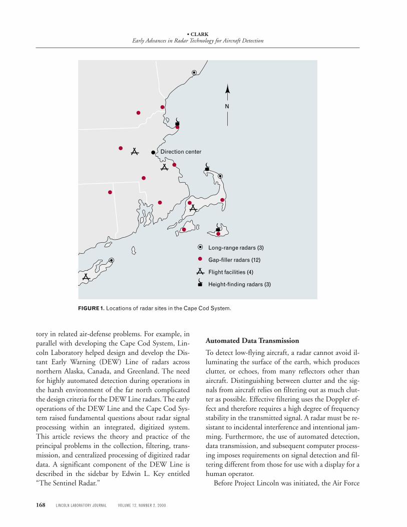
This was an exciting era in the life of the Labora-tory, with a talented and highly motivated staff, a can-do spirit, and minimum administrative formality. AnAir Force unit at nearby Hanscom Field providedsubstantial logistic support. Project Lincoln set up anexperimental air-defense sector called the Cape CodSystem in southeastern New England, as shown inFigure 1. The initial long-range radar for the Cape

Cod System, the AN/FPS-3, was an L-band radarwith a nominal range of 200 miles on a high-flyingbomber. Low-flying aircraft could evade the coverageof the AN/FPS-3 by staying below its horizon. Gap-filler radars, assembled mostly from World War IIcomponents, operated at S-band with a nominalrange of 32 miles. Later, the Cape Cod System wasextended to include additional long-range radars atMontauk Point in Long Island and at West Bath,Maine. These radars supplied only range and azimuthcoordinates. The heights of designated targets weremeasured separately by a small number of height-finder radars.

Data from all the radars were transmitted over or-dinary leased telephone lines to a command center inCambridge, Massachusetts, where the Whirlwindcomputer, and later the system prototype AN/FSQ-7in Lexington, Massachusetts, processed the data inreal time to track aircraft, assist operators to performcommand functions, and guide manned interceptors.The defense system that grew out of this effort wascalled the Semi-Automatic Ground Environment(SAGE). Developing SAGE was the major activityduring Lincoln Laboratory’s early years [2].

The SAGE system also engaged Lincoln Labora-



168 LINCOLN LABORATORY JOURNAL VOLUME 12, NUMBER 2, 2000

N

Direction center

Long-range radars (3)

Gap-filler radars (12)

Flight facilities (4)

Height-finding radars (3)

FIGURE 1. Locations of radar sites in the Cape Cod System.

tory in related air-defense problems. For example, inparallel with developing the Cape Cod System, Lin-coln Laboratory helped design and develop the Dis-tant Early Warning (DEW) Line of radars acrossnorthern Alaska, Canada, and Greenland. The needfor highly automated detection during operations inthe harsh environment of the far north complicatedthe design criteria for the DEW Line radars. The earlyoperations of the DEW Line and the Cape Cod Sys-tem raised fundamental questions about radar signalprocessing within an integrated, digitized system.This article reviews the theory and practice of theprincipal problems in the collection, filtering, trans-mission, and centralized processing of digitized radardata. A significant component of the DEW Line isdescribed in the sidebar by Edwin L. Key entitled“The Sentinel Radar.”

Automated Data Transmission

To detect low-flying aircraft, a radar cannot avoid il-luminating the surface of the earth, which producesclutter, or echoes, from many reflectors other thanaircraft. Distinguishing between clutter and the sig-nals from aircraft relies on filtering out as much clut-ter as possible. Effective filtering uses the Doppler ef-fect and therefore requires a high degree of frequencystability in the transmitted signal. A radar must be re-sistant to incidental interference and intentional jam-ming. Furthermore, the use of automated detection,data transmission, and subsequent computer process-ing imposes requirements on signal detection and fil-tering different from those for use with a display for ahuman operator.

Before Project Lincoln was initiated, the Air Force



Cambridge Research Laboratory in Cambridge, Mas-sachusetts, developed a method called Slowed-DownVideo (SDV) that serves in this discussion as a genericmodel of automated detection. In SDV, range-gateddata from a scanning radar are digitized with a singlebinary digit per range gate. A one value represents athreshold crossing by the signal plus noise and a zerovalue represents no crossing. Within each range gatethe ones were counted in a sliding window as the ra-dar beam scanned a target. At typical scan rates the ra-dar beam stayed on a target long enough for a dozenor more pulse returns from that target. A sufficientnumber of ones within a window represented a targetdetection and triggered a detection signal that wastransmitted over the telephone line. Digits represent-ing detections or nondetections for every range gateand every beamwidth were transmitted sequentiallywithin the bandwidth of the telephone line. This pro-cess yielded data at the receiving end suitable forcomputer processing and generating a digitized ver-sion of the radar display. (See also the article entitled“Radar Signal Processing,” by Robert J. Purdy et al.,in this issue.)

A form of digital signal integration can be simplycharacterized for this discussion by considering a slid-ing window observing a single range gate. A countertotals the threshold crossings within the window. Adetection occurs when a designated number of

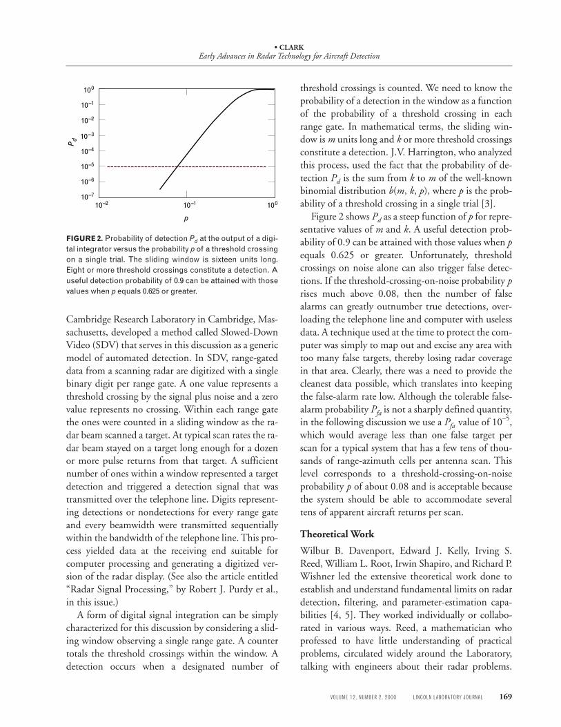
threshold crossings is counted. We need to know theprobability of a detection in the window as a functionof the probability of a threshold crossing in eachrange gate. In mathematical terms, the sliding win-dow is m units long and k or more threshold crossingsconstitute a detection. J.V. Harrington, who analyzedthis process, used the fact that the probability of de-tection Pd is the sum from k to m of the well-knownbinomial distribution b(m, k, p), where p is the prob-ability of a threshold crossing in a single trial [3].

Figure 2 shows Pd as a steep function of p for repre-sentative values of m and k. A useful detection prob-ability of 0.9 can be attained with those values when pequals 0.625 or greater. Unfortunately, thresholdcrossings on noise alone can also trigger false detec-tions. If the threshold-crossing-on-noise probability prises much above 0.08, then the number of falsealarms can greatly outnumber true detections, over-loading the telephone line and computer with uselessdata. A technique used at the time to protect the com-puter was simply to map out and excise any area withtoo many false targets, thereby losing radar coveragein that area. Clearly, there was a need to provide thecleanest data possible, which translates into keepingthe false-alarm rate low. Although the tolerable false-alarm probability Pfa is not a sharply defined quantity,in the following discussion we use a Pfa value of 10–5,which would average less than one false target perscan for a typical system that has a few tens of thou-sands of range-azimuth cells per antenna scan. Thislevel corresponds to a threshold-crossing-on-noiseprobability p of about 0.08 and is acceptable becausethe system should be able to accommodate severaltens of apparent aircraft returns per scan.

Theoretical Work

Wilbur B. Davenport, Edward J. Kelly, Irving S.Reed, William L. Root, Irwin Shapiro, and Richard P.Wishner led the extensive theoretical work done toestablish and understand fundamental limits on radardetection, filtering, and parameter-estimation capa-bilities [4, 5]. They worked individually or collabo-rated in various ways. Reed, a mathematician whoprofessed to have little understanding of practicalproblems, circulated widely around the Laboratory,talking with engineers about their radar problems.

FIGURE 2. Probability of detection Pd at the output of a digi-tal integrator versus the probability p of a threshold crossingon a single trial. The sliding window is sixteen units long.Eight or more threshold crossings constitute a detection. Auseful detection probability of 0.9 can be attained with thosevalues when p equals 0.625 or greater.

100

10–1

10–2

10–3

10–4

10–5

10–6

10–7

10–2 10–1

p

Pd

100



, the UnitedStates decided to deploy a line ofradars across northern Alaska,Canada, and Greenland to pro-vide early warning of a possibleUSSR bomber attack on NorthAmerica. This warning systemwas the Distant Early Warning(DEW) Line. From the outset, thelogistical support of radars in suchremote locations was problematicand expensive. Because air trafficin these extreme northern regionswas light, however, the architectsof the DEW Line felt that con-stant observation of radar screensby human operators was unneces-sary. Consequently, they plannedfor the radars to be unattendedexcept when aircraft were actuallypenetrating the warning zone.This arrangement was achieved byproviding automatic alarms toalert operators when aircraft de-tection occurred. Upon suchalerts, the operators could moni-tor the radar displays and evaluatethe observed circumstances forpotential threats. Since the opera-tors did not need to constantlyattend the radar, they were largelyfree to perform routine site dutiesthat would otherwise require ad-ditional personnel.

Lincoln Laboratory designedthe experimental automatic alarmsystem that was used on the modi-fied AN/TPS-1D radar, whichlater became the AN/FPS-19.

(See the article entitled “DistantEarly Warning Radars: The Questfor Automatic Signal Detection,”by F. Robert Naka and William W.Ward, in this issue.) Because thedesign was for an existing radarwith parameters not optimum forthe purpose, the results were notentirely satisfactory. These short-comings motivated Herbert G.Weiss to design and advocate anew radar that better served the re-quirements for automatic detec-tion. The concept was approved,and in 1954 Lincoln Laboratorybegan the development. The newradar, called Sentinel, was com-pleted and went on the air for test-ing at Lexington in 1955. It incor-

porated in a unified system designmany of the innovations that aredescribed in the accompanyingarticle. Table A shows the majorparameters of the Sentinel radar.

The Sentinel radar incorpo-rated several unusual features forthat time. These novel featuresresulted from the requirementthat it be essentially unattended.The radio-frequency (RF) powersource was a high-gain four-cavityklystron amplifier, which em-ployed a special modulating an-ode to pulse the beam. Theklystron in conjunction with twovery stable oscillators providedhigh-quality coherence for cluttercancellation and velocity filtering.

Table A. Parameters of the Sentinel Radar

RF frequency 570–630 MHz

Peak power 150 kW

Average power 3 kW

Pulse length 40 µsec (detection)5 µsec (threat analysis)

Pulse compression

Barker 13-segment code 39 µsec

compressed to 3 µsec

Transmitter output tube Klystron with62-dB gain

Pulse-repetition frequency 500 pulse/sec

Receiver noise figure <6.5 dB

Antenna aperture 45 ft × 25 ft

T H E S E N T I N E L R A D A REdwin L. Key



The crystal-controlled RF (540 to600 MHz) stable local oscillator(STALO) was the rock on whichSentinel’s frequency stabilityrested. The coherent local oscilla-tor (COHO) was a crystal-con-trolled 30-MHz oscillator. Its out-put was added to the STALO’soutput to provide transmitter ex-citation (570 to 630 MHz). TheCOHO signal was also used as thephase reference for filtering theecho signals after they had beendownshifted to an intermediatefrequency of 30 MHz plus Dop-pler shift by mixing the RF echoeswith the STALO signal.

The pulse-repetition frequency(PRF) was 500/sec to provide alarge unambiguous velocity rangefor velocity filtering to reject re-turns from migrating birds thatwere a problem in the Arctic. ThePRF limited the unambiguousrange to 162 nm, but since thepurpose of the radar’s operationwas to provide a “trip-wire”-likewarning, this was not a concern.Within this limited unambiguousrange Sentinel had a substantialdetection margin to allow for deg-radation. The pulse length fornormal warning operation was 40µsec to provide high pulse energyfor detection and to completely

cover the unambiguous rangewith 50 range gates. After detec-tion the pulse length could be re-duced to 5 µsec for threat analysis.The Sentinel radar was an earlyapplication of pulse compression,which had both theoretical andpractical significance.

It was recognized that the 40-µsec pulse would result in ratherlarge clutter power within a range-azimuth resolution cell, but thecorresponding transmitted pulseenergy was required for detectionperformance. Introducing phase-coded compression similar to thatused in the AN/FPS-17 radar al-lowed the radar to transmit a longpulse while achieving range reso-lution that corresponded to ashort transmitted pulse. (For a dis-cussion of the AN/FPS-17 radar,see the article entitled “Radars forthe Detection and Tracking ofBallistic Missiles, Satellites, andPlanets,” by Melvin L. Stone andGerald P. Banner, in this issue.) Asimple Barker 13-segment phase-reversal code was designed for theSentinel radar to test whetherpulse compression could reduceclutter. The pulse-compressionwaveform consisted of a 39-µsecpulse with 3-µsec subpulses codedwith a particular sequence of

phase reversals, providing 13-to-1compression. Once the clutter-re-duction claims were verified, re-searchers included pulse compres-sion in the Sentinel radar’s design.

The Sentinel radar was ac-quired by the Air Force, renamedthe AN/FPS-30, and manufac-tured by Bendix. The AN/FPS-30was deployed by the Air Force inthe extension of the DEW Lineacross southern Greenland. It wasreported that the pulse compres-sion proved to be the savior of thesystem. Sometimes a large ice floeoff the coast of Greenland pro-duced clutter returns with a 40-µsec pulse that exceeded thesubclutter-visibility capabilities ofthe radar. However, the 13-to-1compression provided enoughclutter reduction for the radar tobe able to see targets.

Edwin L. Key joined Lincoln Laboratoryin 1951 and contributed to a variety ofradar programs, including SAGE, theDEW Line, BMEWS, and the MillstoneHill facility. He transferred to the MITREcorporation upon its formation in 1959.At MITRE, he held positions of increasingresponsibility that culminated in his posi-tion as senior vice president for researchand engineering. Although retired, he con-tinues to consult in the areas of radar sys-tems, radar technology, signal processing,and communication systems.

These discussions often gave him the idea for ananalysis that he could perform. Then, in useful cross-fertilization, he would report back on his analyticalresults to the engineer who had inspired the idea. Hewas one of the more prolific authors of technical re-ports in the early days of the Laboratory. One of hismajor contributions to the digital-processing com-munity is the origination of the Reed-Solomon error-

correction algorithm, which is discussed at the end ofthis article.

A significant problem under investigation duringthis time involved signal integration. Our earliestknowledge of signal integration came from RubyPayne-Scott [6], J.I. Marcum [7] and John V. Har-rington [3]. Confusion existed about the relative ad-vantages of noncoherent integration and coherent in-



tegration. Over a period of time, with contributionsfrom several people, we learned that coherent integra-tion can offer a substantial advantage, especially forsignal-to-noise ratios near unity or lower. The advan-tage is greatest when we know precisely the frequencyof the signal being integrated. The advantage is re-duced somewhat when the signal can have a range offrequencies, as with Doppler frequencies from mov-ing targets with unknown velocities.

Another problem at the time was establishing howaccurately a radar could estimate various target pa-rameters such as range, velocity, acceleration, and azi-muth and elevation angle. Several people within theLaboratory, including Kelly, Roger Manasse, Reed,and Root, and others outside the Laboratory, includ-ing P. Swerling, addressed the problem. Their work,and that of others, is well summarized by Swerling inchapter 4 of Merrill I. Skolnik’s Radar Handbook [8].

Chaff, consisting of many small scatterers, was acountermeasure used widely in World War II to con-fuse enemy radars. Kelly treated extended targets likechaff and precipitation with a mathematical modelfor the radar echo as coming from a random collec-tion of scatterers, necessarily highly idealized [9].

The characteristics of the chaff radar echo dependupon the distribution of the scatterers, their bulk mo-tion, and their motion relative to each other, as well ason the characteristics of the radar pulse that illumi-nates them. The radar echo from many scatterers hasnoiselike qualities and coherent qualities. Dependingon the wind, the Doppler frequencies can be highenough to seriously compromise Doppler-filteringschemes. Wind shear or turbulence can generate aspread of Doppler frequencies that further compli-cates the job of filtering. Changing the radar fre-quency randomly from pulse to pulse can destroy thecoherence of the echo. (A way of exploiting this fact isbriefly described later.) Other sources provide a moredetailed account of this theoretical work [9–13].

Looking to the future, well beyond air defense,Shapiro studied the ability of radars to predict ballis-tic missile trajectories. His monograph proved to bethe defining work on this subject [13]. Shapiro thenturned his attention to radar astronomy, and he hashad a distinguished scientific career at MIT and at theSmithsonian Astrophysical Observatory.

Characterization of Clutter

The author’s acquaintance with radar clutter began inthe summer of 1952 under the guidance of Robert C.Butman, an experienced radar engineer. We had theuse of an experimental S-band radar located on theroof of MIT’s tallest building. It had a good view ofthe area surrounding Cambridge, which included Lo-gan Airport and Hanscom Field. We spent manyhours observing air traffic and clutter, and experi-menting with the Doppler-filtering moving-target in-dicator (MTI). In principle, MTI filtered out cluttersignals from stationary and near-stationary reflectorswhile passing signals from aircraft having significantradial velocities with respect to the radar. A rough butuseful judgment of the ability of the MTI to rejectclutter could be made by comparing a plan positionindicator (PPI) display of the unfiltered radar scenewith a display produced by the MTI. Much less obvi-ous was the radar’s ability to follow an aircraftthrough a heavily cluttered area. At one point But-man, taking advantage of Air Force logistic support,arranged for a flight test to start learning somethingabout that ability. At the appointed time a trainer air-craft appeared and circled our site. Butman estab-lished contact by using a war-surplus radio. He re-quested the pilot to fly over a heavily cluttered areanorthwest of the radar to see how well the MTI couldpick the aircraft out of the clutter. When the aircraftwas lined up on the desired course he asked the pilotto continue flying in that direction until he receivedfurther instructions. At that point our radio emittedclouds of smoke and died. Such was the author’s in-troduction to flight tests.

The twelve gap-filler sites of the Cape Cod Systemprovided an opportunity to study a variety of clutter.An instrument called the MTI Site Evaluator wasconstructed and brought to each site to observe clut-ter in conjunction with the MTI. Unfortunately, thename of the device initially terrified some of the sitetechnicians. The instrument mapped areas where air-craft might be obscured by strong background clutter.After the survey of all sites, the site with the largestand most intensely obscured area was selected for aflight test. A medium bomber, following radio in-struction from the site, was tracked on the radar dis-



play as it flew over what appeared to be the most se-verely obscured area. It proved difficult to find an areawhere the echo from the bomber was obscured formore than a scan or two. This finding was consistentwith observations of aircraft targets at other sites. Atthe time, we concluded that very intense clutter ech-oes were due to specular reflections from fixed targetsof limited areal extent, such as tall buildings and wa-ter towers. If filtered out by the MTI they were notlikely to negate the ability of the radar to track largeaircraft. The term interclutter visibility was later usedto describe this ability to track objects in areas ofstrong background clutter.

Some limited observations were made with an S-band radar on echoes from rain and chaff. Observa-

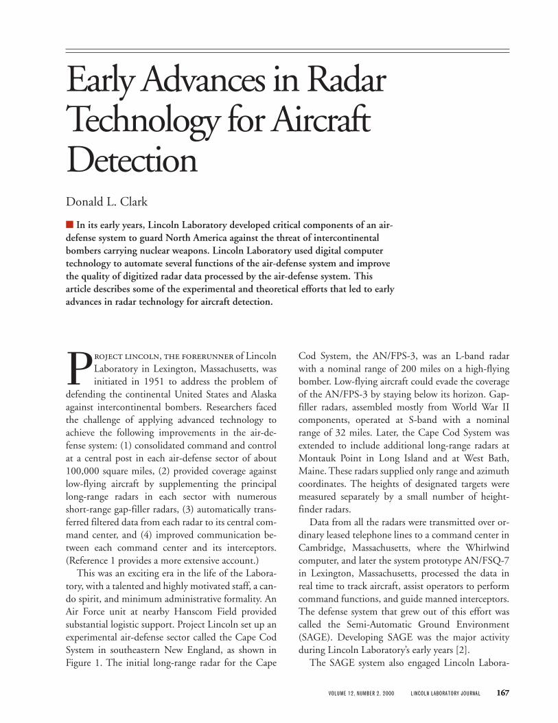
tions consisted of numerous Doppler spectra mea-sured within a single range gate with the antennapointed to the region of interest. Figures 3(a) and3(b) show sample spectra from rain and from chaff,respectively. Both spectra were found to be highlyvariable, depending upon wind conditions. A spec-trum from a C-45 aircraft inbound is shown in Figure3(c). Either rain or chaff could have Doppler frequen-cies overlapping those expected from aircraft, therebyseriously complicating the task of Doppler filtering.

These limited observations of clutter left much tobe desired. They provided only a qualitative basis fordesigning filtering schemes. A proper characterizationof clutter awaited another era, when low-altitude,low-cross-section cruise missiles were the driving con-cern. (See the article entitled “Radars for the Detec-tion and Tracking of Cruise Missiles,” by Lee O.Upton and Lewis A. Thurman, in this issue.)

Clutter Filtering

The principal technique initially available for dealingwith radar clutter was MTI. In this scheme, theradar’s phase-detected video signal was delayed by oneinterpulse interval and subtracted from the next videosignal. The signal from a stationary target such as awater tower would be effectively canceled. The signalfrom a target having a significant radial velocity withrespect to the radar would be Doppler-shifted and, ingeneral, would not cancel. Chapter 17 of Skolnik’sRadar Handbook offers a useful discussion of this typeof MTI [14]. During our experiments, the signal wasdelayed as a sound wave propagating through a col-umn of mercury driven by a piezoelectric transducer.With careful adjustment, sharp nulls could be at-tained on stationary targets, but they were hard tomaintain due to temperature changes and other insta-bilities of the delay line. Effort was directed at devel-oping better means of delaying the video signal. Afterconsiderable trial and error, the best approach wasfound to be the use of a delay line in which the soundwave followed a folded path within a slab of fusedquartz. A cancellation null depth of 37 dB was even-tually demonstrated, with excellent stability.

The filter response of this type of MTI had theform of a rectified sine wave with peaks at odd mul-tiples of half the pulse-repetition frequency (PRF)

FIGURE 3. (a) Doppler spectrum of rainstorm echoes ob-served with an S-band radar. (b) Doppler spectrum of chaffechoes observed with an S-band radar. (c) Doppler spec-trum of a C-45 aircraft inbound observed with an S-bandradar.

(a)

10 500

(b)

500

(c)

10 1500

Rel

ativ

e in

tens

ityR

elat

ive

inte

nsity

Rel

ativ

e in

tens

ity

Frequency (Hz)

Frequency (Hz)10

Frequency (Hz)



and nulls (blind speeds) at multiples of the PRF. (Ablind speed occurred when the target moved radiallyan integral number of half wavelengths in oneinterpulse period.) Other approaches to Doppler fil-tering were tried that offered some flexibility in shap-ing the filter response. In one approach, coherentvideo was range-gated and filtered with an analog fil-ter for each range gate. In another approach, ThomasC. Bazemore and Bruce Nelson saved the polarities ofthe range-gated coherent video as a sequence of bi-nary digits in a shift register. A diode or resistor arrayattached to the shift register allowed periodicities thatcorrespond to Doppler frequencies to be detected. Ineffect one had a bank of elementary digital filters in asliding window. This scheme was tested with a fewrange gates on an S-band radar. Although it showedpromise, the digital technology available at that timerequired one vacuum tube flip-flop per binary digit,which made a full-scale implementation impractical.

John P. Perry and the author investigated anotherapproach to Doppler filtering called “Sinufly,” a tech-nique borrowed from C.W. Sherwin at the Coordi-nated Science Laboratory of the University of Illinois.This technique used a storage tube similar to a cath-ode-ray tube except that an electrostatic storage sur-face replaced the phosphor on the face of the tube.The electron beam, modulated by radar video, wasscanned in a raster across the storage surface, layingdown a pattern of electric charge. When the surfacewas completely scanned, the unmodulated beam wasscanned in a raster at right angles to the first to readout the stored electric charge. This arrangement hadthe effect of range-gating the video and allowing theDoppler frequencies, multiplied by a large factor, tobe read out sequentially, range gate by range gate. Byswitching between two tubes all of the radar videocould be captured. With this scheme a single bank offilters was shared among all range gates, which per-mitted experimentation with various filteringschemes. The system had many attractive features butwas limited by the inadequate dynamic range of thestorage tubes that we used. The tubes were laboratorysamples that were never further developed; hence wehad to abandon this scheme.

Although we explored a variety of ideas for clutterfiltering, we found that many sophisticated ap-

proaches could not be reasonably supported by thememory technology available at the time [15]. Thebest memory available to us in this era was the quartzdelay line. A demonstration system exploiting quartzdelay lines is described briefly below. A small mag-netic-core memory, which provided some interestingpossibilities, arrived too late to be fully exploited.

Jamming and Interference

Andrew Bark and Robert Bergemann, working on ra-dar countermeasures, demonstrated with a jammerdeveloped during World War II the radar problemscaused by jamming or by incidental interference. Thejammer consisted of a mechanically tunable continu-ous-wave (CW) magnetron that radiated through asmall horn antenna in the tail of a test aircraft. Its fre-quency could be swept rapidly back and forth across abroad band and its signal was sufficiently strong topenetrate the sidelobes of the radar antenna as well asthe main lobe. When swept through the radar fre-quency band, it produced a strong signal that clut-tered the display and reduced the radar’s sensitivity.With automated detection, it overwhelmed the sys-tem with false alarms.

A remedy, suggested by Robert H. Dicke during anearlier study, was to limit or clip the amplitude of aradar signal. This technique became known as theDicke Fix. (Actually, the idea of clipping signal ampli-tude to reduce the effects of interference was a newapplication of an old idea. Radio hams had alreadybeen reducing interference effects in their receiversthis way.)

We explored several methods for clipping the am-plitude of a signal. The simplest, and one of the mosteffective variations, was to use a wideband intermedi-ate-frequency (IF) amplifier with a hard limiter fol-lowed by a narrowband filter and rectifier. A hardlimiter amplified the receiver noise to drive the lim-iter to saturation, so that there was negligible varia-tion of the amplitude at its output with or withoutsignal or interference present. The narrowband filterresponded more strongly to the radar signal than tonoise, allowing aircraft to be detected. In this context,narrowband meant a bandwidth matched to the radarpulse; wideband meant bandwidth several (e.g., ten)times greater.



A receiver using a technique like this was found byexperiment to be much more resistant to jammingand interference than a more conventional non-limit-ing receiver. A major frustration at the time was thelack of an analytical model to describe the effects wewere seeing experimentally. Such a model was devel-oped some forty years later and is described in thenext section.

Analytic Performance of a Hard-Limiting Receiver

An example using a simple analytic model of a hard-limiting receiver can help us to understand the hard-limiting receiver and to compare it with a conven-tional linear receiver. In this model, a wideband filterprecedes the narrowband filter, where the ratio ofbandwidths is n. The narrowband filter is thus pre-sented with n independent samples of noise passed bythe wideband filter, plus the signal (if present). Thenoise is modeled as having random phase over 360°and a Gaussian amplitude distribution with zeromean and unit variance. The narrowband filter, tunedto the signal frequency, adds the n samples. The noiseadds noncoherently; the signal, having constant phase(modulo 2π), adds coherently. In the linear receiver athreshold is set such that when the threshold is ex-ceeded, the receiver puts out a one, otherwise, a zero.In the hard-limiting receiver, each of the n samples islimited to unit amplitude, with phase the same as thatof the signal plus noise of the linear receiver. We canpicture these samples as n unit vectors that add in ran-dom-walk fashion when noise predominates, and thatline up to add in phase when signal predominates.Again, a threshold is set to produce a one when ex-ceeded and a zero otherwise. (For an analytical discus-sion of related ideas see Reference 16.)

This model was implemented in a program thatgenerated n samples of signal plus noise, as described.The resulting n vectors were added for each receiver,and the amplitude of the result was compared to afixed threshold for each. By repeating this processmany times Monte Carlo fashion, we could estimatethe probability p of detection/false alarm per rangegate. Using the binomial formula referred to earlierwe could calculate the probability of (apparent) de-tection P after digital integration.

Interference and/or jamming were modeled as a

probability pI that a noise sample would be takenfrom a distribution with variance I many times that ofthe noise, but otherwise similar. This probability pIcould be chosen anywhere in the range from 0 to 1.

Figure 4 shows the behavior of the two types of re-ceiver with fixed thresholds set to produce a probabil-ity p of about 0.08 for a threshold crossing on noisealone. As pI was increased, the false-alarm probabilityPfa was observed for values of I that are 10 and 100times the noise. Figure 4 shows that the hard-limitingreceiver maintained Pfa at about 10–5 for all values ofpI. It is clear that the linear receiver produced intoler-able false-alarm probabilities by the criterion de-scribed earlier in this section for pI greater than about10–2. The curves shown are somewhat irregular, dueto the limited statistics of the Monte Carlo model.

The threshold for the linear receiver can be ad-justed to keep its false-alarm probability nearly con-stant as pI is changed. The threshold has to be raisedsubstantially as pI increases to maintain the false-alarm probability, thereby desensitizing the receiver.We can then observe the probability of detection witha signal present. Figure 5 shows Pd as a function of pIfor a signal whose peak amplitude was the square rootof 10 times the variance of the wideband noise. Thecurves shown are for I equal to 100 times the noise. Itis apparent that the linear receiver lost its ability to

FIGURE 4. Probability of false alarm Pfa versus probability ofinterference pI. The black curve represents data from a linearreceiver with interference 100 times the noise. The red curverepresents data from a linear receiver with interference 10times the noise. The blue curve represents data from a hard-limiting receiver with interference 10 times the noise. Onlythe hard-limiting receiver maintains a Pfa value of 10–5 for allvalues of pI.

100

10–1

10–2

10–3

10–4

10–5

10–6

10–7

10–3 10–2

pI

10–1

Pfa

100



detect the signal at small values of pI. The hard-limit-ing receiver maintained a useful detection probabilityfor values of pI up to about 0.4, for the combinationof parameters chosen.

To summarize, in the presence of intense interfer-ence the linear receiver either produced too manyfalse alarms or became desensitized. The hard-limit-ing receiver, by contrast, maintained a constant lowfalse-alarm probability, together with useful sensitiv-ity in the presence of severe interference. Franklin A.Rodgers, who briefly led the group in which this workwas done, described the class of receivers in our ex-periments as constant false-alarm rate (CFAR), whichwas also a play on Rodgers’s initials.

Performance of Actual Receivers

Figure 6 shows a practical comparison of two actualreceivers subjected to jamming. Figure 6(a) shows atime exposure of an output display of a linear receiversubjected to severe jamming from three airborne jam-mers on a single plane. Figure 6(b) shows a time expo-sure of an output display of a hard-limiting receiverunder the same conditions. The hard-limiting re-ceiver in this case used wideband video with a zero-crossing counter. The lines of blips represent aircrafttracks. The results are consistent with the results ofthe analytical model described above.

Some time after we had achieved the results brieflydescribed above, we learned that D. Griffin at Har-

vard University had made some interesting observa-tions of the ability of bats to rely on their sonar tonavigate and capture insects. In particular, he hadtested bats in the presence of interfering noise, andthey appeared to have an astonishing capability to re-sist the noise. Had we overlooked something that thebats could teach us?

The Laboratory arranged to have J.J. GeraldMcCue, assisted by David A. Cahlander, work withGriffin to follow up on his observations in more de-tail. They set up a carefully instrumented enclosure inwhich the bats could fly freely. Instrumentation in-cluded a strobe light and high-speed movie camera tophotograph the bats in flight, a microphone and re-cording system to record their chirps, and an adjust-able noise generator that filled their enclosure withcontinuous near-white noise to jam their sonar. Mov-ies of flying bats were played back in slow motion.Recorded chirps were synchronized with the movieand slowed down sufficiently to bring the chirpswithin human audible range. The movies and soundprovided a graphic and convincing way of observingthe bats. It was an enjoyable project whose propensityto grow had to be restrained. We learned that, alas,the bats had no more ability to resist jamming thancould be accounted for by existing models [17–19].

Master-Oscillator/Power-Amplifier Transmitter

The earliest microwave radars used magnetrons togenerate the power required for the transmitter. Mag-netrons have an honorable history as the inventionthat made possible the development of microwave ra-dar during World War II. Magnetrons operated asself-excited oscillators whose characteristics, however,left something to be desired. Early in the life of Lin-coln Laboratory an arrangement was worked out withthe Physics Department at Stanford University andwith Varian Associates to supply two S-band klys-trons, with spares, to the Laboratory. Butman andGordon L. Guernsey used these klystrons in anS-band amplifier chain to generate 1 MW of peakpower and 2 kW of average power. Their driving os-cillator was a low-power klystron whose frequencywas stabilized by a very high-Q cavity. The klystronswere thoroughly tested, and they found extensive usein an experimental radar at the Laboratory, where

FIGURE 5. Probability of detection Pd at the output of a digi-tal integrator versus the probability of interference pI. Inter-ference was 100 times noise. Peak signal amplitude was thesquare root of 10 times the wideband noise variance.

100

10–1

10–2

10–3

10–4

10–5

10–6

10–7

10–3 10–2 10–1

pI

Pd

100

Hard-limiting detector

Linear detector



they demonstrated stable, reliable, and highly coher-ent operation—a large improvement over the opera-tion of the magnetron.

Somewhat later Butman and Guernsey tested a six-cavity klystron developed by Varian Associates forHughes Aircraft Company. For this application, thecavities were stagger-tuned for broad bandwidth atthe expense of gain. In the Lincoln Laboratory teststhe six cavities were synchronously tuned to maxi-mize the gain. A stable gain of 89 dB was attainedwith root-mean-square phase fluctuation under2.5°—a remarkable result at that time.

These tests marked the beginning of what came tobe an extensive program in which Butman, Guernsey,and Clarence W. Jones worked with industry to de-velop high-power microwave components and to testnumerous high-power klystrons for a variety of appli-cations. The development of klystrons opened up thepossibility, exploited in a later era, of using a variety ofradar waveforms on demand, such as frequency-modulated pulses for pulse compression and shortbursts of closely spaced pulses to permit measurementof very high Doppler frequencies.

Demonstration of an Integrated Radar System

To cap off the work described above we combined

several techniques into an integrated demonstrationsystem. The key idea for the system, proposed byMartin Axelbank, was an unusual form of signal inte-gration. He observed that the hard-limited echo froman extended target, such as chaff or precipitation, isdecorrelated (i.e., becomes noiselike) if the radar fre-quency jumps at random from pulse to pulse. By con-trast, the echo from a large target, such as an aircraft,has a component that remains steady from pulse topulse. Integration, necessarily noncoherent, could en-hance the signal of an aircraft relative to that of com-peting chaff or precipitation, thereby yielding a tech-nique later called superclutter visibility.

The system used a two-pulse delay-line MTI, aquartz delay-line analog integrator, and a transmitterthat randomly jumped frequency over a broad bandof frequencies after each pair of pulses. The combina-tion of the hard-limiting receiver and frequencyjumping made the radar highly resistant to jamming.The two-pulse MTI used a short interpulse periodthat broadened the filter null around zero Dopplerfrequency and moved the first blind speed out to ahigh value, which provided reasonably good Dopplerfiltering. The analog integrator in combination withthe frequency jumping was effective in filtering outchaff and rain clutter. This system was as successful as

FIGURE 6. Comparison of displays from two receivers subjected to three jammers on a single B-47 at35,000-ft altitude and 10-mi range: (a) time exposure of an output display of a linear receiver and (b) timeexposure of the output of a hard-limiting receiver. The lines of blips represent aircraft tracks.

(a) (b)



any that we tried. We could not test it at length, how-ever, because other radar operators nearby were dis-tinctly unenthusiastic about the interference effectson their radars of its frequency-jumping mode.

Error Correction

Finally, attention should be called to some work onerror correction, somewhat out of the main stream ofradar research. As pointed out above, the Cape CodSystem transmitted digitized radar data over tele-phone lines. At that time, digitized data transmissionwas a largely undeveloped art. Telephone lines thatwere adequate for voice signals were often far less thanideal for digital signals, resulting in significant errorsin the received signals. This inadequacy motivated aninvestigation of how to reduce errors.

Irving S. Reed and Gustave Solomon investigateda number of mathematical schemes with potential forerror correction. Their work culminated in publica-tion of a fundamental and rather abstract mathemati-cal paper in the Journal of the Society for Industrial andApplied Mathematics [20]. Although their paper waslittle noticed at the time, it contained basic ideas thathave since been developed into powerful and widelyused error-correction schemes, now known as Reed-Solomon error-correcting codes [21]. The codes havebeen used with compact discs, digital audio tape,high-definition TV systems, and the Voyager andGalileo spacecraft. Reed and Solomon received the1995 IEEE Masaru Ibuka Consumer ElectronicsAward for this work.

Retrospective

As the digital-computer technology needed for theSAGE system matured, the MITRE Corporation wasset up in 1958 to oversee the implementation of thesystem in the field. Related work at Lincoln Labora-tory was attenuated. The imminent advent of inter-continental ballistic missiles and the launch of Sput-nik I further dampened interest in research onair-defense techniques. The work on radar from theLaboratory’s first several years, described above, didnot have the practical impact on air-defense radarsthat it might have had otherwise. One fruitful result,however, was the education of a cadre of people atLincoln Laboratory in both the underlying theory of

radar detection and parameter estimation and in thenitty-gritty of practical applications, preparing themto take on new and greater challenges.

Acknowledgments

I am indebted to the caretakers of the Lincoln Labo-ratory archives for help in finding early Lincoln Labo-ratory reports and copying pertinent excerpts.



R E F E R E N C E S1. A.G. Hill, J.W. Forrester, and G.E. Valley, “Quarterly Progress

Report, Division 2—Aircraft Control and Warning, Division6—Digital Computer,” 1 June 1952. (This report was thefirst in a long series of quarterly progress reports. Some infor-mation from later reports in the series has also been used here.)

2. E.C. Freeman, ed., MIT Lincoln Laboratory: Technology in theNational Interest (Lexington, Mass., 1995), pp. 15–33.

3. J.V. Harrington, “An Analysis of the Target Detection of Re-peated Signals in Noise by Binary Integration,” IRE. Trans. Inf.Theory 1 (1), 1955, pp. 1–9.

4. W. L. Root, “Remarks, Mostly Historical, on Signal Detectionand Signal Parameter Estimation,” Proc. IEEE 75 (11), 1987,pp. 1446–1457

5. W.B. Davenport, Jr., and W.L. Root, An Introduction to theTheory of Random Signals and Noise (McGraw-Hill, New York,1958).

6. R. Payne-Scott, “The Visibility of Small Echoes on PPI Dis-plays,” Proc. IRE 36 (2), 1948, pp. 180–196.

7. J.I. Marcum, “A Statistical Theory of Target Detection byPulsed Radar, and Mathematical Appendix,” IRE Trans. Inf.Theory 6 (2), 1960, pp. 59–267 (originally published asRAND Corp. Res. Mem. RM-754, 1 Dec. 1947, and RM-753, 1 July 1948).

8. P. Swerling, “MTI Radar,” in Radar Handbook, M.I. Skolnik,ed. (McGraw-Hill, New York, 1970), pp. 4.1–4.14.

9. E.J. Kelly, I.S. Reed, and W.L. Root, “The Detection of RadarEchoes in Noise,” SIAM J. 8 (2), 1960, pp. 309–341, andSIAM J. 8 (3), 1960, pp. 481–507.

10. E.J. Kelly, “The Radar Measurement of Range, Velocity andAcceleration,” IRE Trans. Mil. Electron. 5 (2), 1961, pp. 51–57.

11. I.S. Reed, “On the Use of Laguerre Polynomials in Treating theEnvelope and Phase Components of Narrow-Band GaussianNoise,” IRE Trans. Info. Theory 5, Sept. 1959, pp. 102–105.

12. R.P. Wishner, “Distribution of the Normalized PeriodogramDetector,” IRE Trans. Info. Theory 8, Oct. 1962, pp. 342–349.

13. I.I. Shapiro, The Prediction of Ballistic Missile Trajectories fromRadar Observations (McGraw-Hill. New York, 1958).

14. W.W. Schrader, “MTI Radar,” in Radar Handbook, pp. 17.1–17.60.

15. J.P. Eckert, Jr., “A Survey of Digital Computer Memory Sys-tems,” Proc. IRE. 41, Oct. 1953; reprinted in Proc. IEEE 85(1), 1997, pp. 184–197.

16. W.R. Bennett, “Methods of Solving Noise Problems,” Proc.IRE 44 (5), 1956, pp. 609–638.

17. D.R. Griffin, J.J.G. McCue, and A.D. Grinnell, “The Resis-tance of Bats to Jamming,” J. Exp. Zool. 152, 1963, pp. 229–250.

18. D.A. Cahlander, J.J.G. McCue, and F.A. Webster, “The Deter-mination of Distance by Echolocating Bats,” Nature 201, 8Feb. 1964, pp. 544–546.

19. J.J.G. McCue, “Aural Pulse Compression by Bats and Hu-mans,” J. Acoust. Soc. Am. 40 (3), 1966, pp. 545–548.

20. I.S. Reed and G. Solomon, “Polynomial Codes over CertainFinite Fields,” SIAM J. 8 (2), 1960, pp. 300–304.

21. B.A. Cipra, “The Ubiquitous Reed-Solomon Codes,” SIAMNews 26 (1), 1993.



. received a bachelor’s degree inelectrical engineering at theUniversity of Vermont in1943. He worked in the re-search laboratory at StrombergCarlson in Rochester, NewYork, mainly on magneticrecording. He earned a Ph.D.degree in physics at the Uni-versity of Rochester, where heexperimented with pi mesons.He joined Project Lincoln in1952 and enjoyed a 31-yearcareer at Lincoln Laboratory.He worked mostly on variousproblems of radars at thecutting edge of technology. Asa result of the experiencedescribed in the article he wasan early advocate for takinginto account during the speci-fication and design phase ofmilitary radar developmentsthe likely countermeasures towhich the radars might besubjected. His group studiedtest-range measurement radars,ballistic-missile-defense radarsand other sensors in a varietyof contexts, and satellite sur-veillance and identificationradars, exploiting—wherepossible—data from theLaboratory’s extensive field-measurements program atKwajalein. His proudest andmost lasting accomplishmentwas bringing a number ofoutstanding people to theLaboratory and helping toguide their careers. He is a lifemember of AAAS and IEEE, asenior member of APS, anemeritus member of AAPT,and a member of Sigma Xi.

Documents

Early Advances in Radar Technology for Aircraft …€¢ CLARK Early Advances in Radar Technology for Aircraft Detection VOLUME 12, NUMBER 2, 2000 LINCOLN LABORATORY JOURNAL 169 Cambridge