TDA Progress Report 42-95

Dynamic Models for Simulation of the 70-M Antenna Axis Servos

R. E. Hill Ground Antenna and Facilities Engineering Section

Dynamic models for the various functional elements of the 70-m antenna axis servos are described. The models representing the digital position controller, the linear and nonlinear properties of the physical hardware, and the dynamics of the flexible antenna structure are encoded in six major function blocks. The general modular structure o f the function blocks facilitates their adaptation to a variety o f dynamic simulation studies. Model parameter values were calculated from component specifications and design data. A simulation using the models to predict limit cycle behavior produced results in excel- lent agreement with field test data from the DSS 14 70-m antenna.

July-September 1988

1. Introduction The recent acquisition of a microcomputer workstation and

a software package for modern control system analysis and simulation has enabled combining the linear dynamics of the antenna structure, the nonlinearities of friction, and the quan- tized, sampled data properties of the control algorithm in a

vides a building block approach to modeling complex systems such as the 70-m antenna axis servos. The models described here were developed from previous linear models [ I ] , [2] in generalized building block forms. The form of the modularity was chosen to maintain generality and to facilitate future expansion or simplification of models for selected parts of the system.

I

I single simulation model. The dynamic simulation program pro-

The 70-m servo models described here are organized accord- ing to function into six major blocks which are shown (Fig. 1) interconnected to represent the overall axis-position servo. The overall model includes the salient properties of the control algorithm, the digital-to-analog converter, the electronic con-

trol amplifier, the hydraulic servovalve, the hydraulic motor with associated friction, the antenna structure and pedestal, and the axis encoder.

II. Dynamic Model Development A. Position Loop Control Algorithm

The structure of the control algorithm is discussed in detail in [ l ] . The estimator and gain equations for the computer mode from [ l ] are repeated here to illustrate the development of the discrete system equations representing the algorithm block.

E ( n t 1 ) = @ E ( n ) + I ' U ( n ) + L Y , ( n t l ) (1 a)

for E, through E,, and

E,(n + 1) = E l ( n ) +E,(n) - R ( n ) (1b)

32

https://ntrs.nasa.gov/search.jsp?R=19890010962 2018-09-03T05:49:51+00:00Z

u(n + 1) = - KE(n + 1) + N R ( n + 1) ( 2 )

- E(n + 1)

U(n + 1)

E,(n + 1) -

where E(n + 1) is the state estimate column vector of [ l ] , [E1 E, E , . . . E6] corresponding to time interval n t 1. In [ l ] the R(n) term in the equation for the integral error esti- mate, E l , was omitted in error.

=

In practice, the antenna servo controller evaluates Eq. ( la) in two steps in order to minimize the computation delay within the servo loop, and implements Eq. ( lb ) to simplify the computation of E, and conserve computing time. Eq. ( lb ) is equivalent to Eq. ( la ) for the special case where the first row of @ is [ l 1 0 0 0 01, the first elements of I' and L are zero, and R(n) is subtracted. Eq. ( la) can thus be extended to the more general form to include E,

whereMis the column vector 0 0 0 0 01.

Next, substituting

and

U(n) = -KE(n) + NR ( n )

into Eq. (3) yields the familiar form for the estimator

E(n + 1) = [ I - L H ] [ a - I ' K ] E ( n ) + L Y ( n + 1)

+ [I-LH]I'NR(n)+MR(n) (4)

With the use of Eq. (4), the controller output U and the posi- tion estimate E, can be expressed in a compact state space form for a system having three inputs and two outputs defined by Eqs. (2) and (3)

where

A B

C D

HA HB

C = - K A

D = [ - K B + [0 0 N I ]

Figure 2 illustrates the control algorithm block with inputs which are the encoder output, Y, and the current position command, R ; its outputs are the rate command, U, and the encoder position estimate, E,. The two blocks shown are standard building blocks provided by the simulation program. The previous rate command, R(k ) , is derived from the unit delay. The discrete time equations represented by the A, B, C, and D matrices are evaluated at 50-msec intervals by the State Space block.

6. Electronic Component Models

The digital-to-analog converter in Fig. 1 is represented by a standard building block which quantizes a continuous input function.

The axis encoder is modeled by a standard quantizer build- ing block from the simulation program catalog as shown in Fig. 1. The quantization level corresponds to 360 degrees per 220 encoder increments.

The amplifier model block shown in Fig. 3 represents the dynamics of the hardware rate and acceleration limiters, the rate loop compensation networks, and the valve driver ampli- fier. Inputs are the rate command from the digital-to-analog converter and the motor rate, and the outputs are the current to the hydraulic valve and the voltage at the average tachom- eter circuit node. Parameter values are calculated from the component values in the schematic diagram,' and the proper- ties of the valve coil. Details of these calculations are included in the Appendix.

C. Hydromechanical Component Models

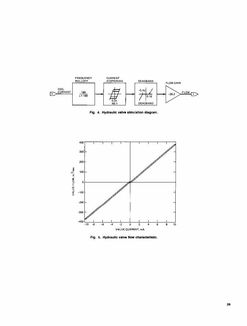
The hydraulic valve model block is shown in Fig. 4 where the input is valve coil current and the output is no-load volu- metric flow. The flow reduction due to the hydraulic pressure of the load is incorporated in the damping term of the motor model. This form of modeling simplifies the block intercon- nections by eliminating a pressure feedback path from the motor block to the valve block. The valve flow versus current is modeled by a simple dynamic lag followed by a hysteresis function and a deadzone. The deadzone corresponds to the underlapped condition of the valve spool face and the hystere-

JPL Drawing J9479871D, Schematic Diagram, Analog D.W.B., (inter- nal document), Jet Propulsion Laboratory, Pasadena, California, 1987.

1

33

sis results from friction associated with the spool motion. The resulting flow characteristic of this model, shown in Fig. 5 , compares well with those from actual valve tests performed by the manufacturer.

B =

where

I - -

0

1 - $1

0

0 - -

1

Figure 6 shows the model of the hydraulic motor where the inputs are the no-load hydraulic flow and the load torque at the antenna bullgear. The outputs are the rate at the bullgear, the rate at the motor shaft, and the differential hydraulic pres- sure. The model incorporates the performance equations described in [ 2 ] and a more accurate model [3] for the fric- tion associated with the motor and the gear reducer.

I D. Flexible Structure Dynamics

A block diagram of the structure dynamic model is shown in Fig. 7. The model includes the gearbox stiffness, the residual structure inertia, axis damping and Coulomb friction, and state space models for the flexible modes of the structure and the antenna pedestal. The residual inertia represents that part of the total axis inertia that is not associated with any of the flexible modes. The inputs correspond to the hydraulic motor rate and an external disturbance torque. The first three out- puts correspond to the angular positions at the bullgear, the axis encoder, and the intermediate reference assembly (IRA), respectively. The fourth and fifth outputs correspond to the axis reaction torque which is reflected back to the motor, and the encoder rate. It should be recognized that the bullgear and IRA positions are in absolute, or inertial, coordinates while the encoder position and rate are measured relative to the pedestal displacement.

I

The model is based on the equations of motion described in [ 2 ] with the addition of axis damping, friction, and pedestal dynamics. A block diagram representation of the structure

is the bullgear angle and the outputs are the IRA angle and the net reaction torque reflected to the bullgear. The correspond- ing state space equations are given by Eq. (6). The flexible alidade structure model, for the elevation axis, is shown in the block diagram of Fig. 8(b) and the corresponding state space equations are given by Eq. (7). The pedestal dynamic equa- tions have the same form as those of the alidade structure used in the elevation model in Eq. (7). Numerical values of the structure parameter are listed in Table 1.

I

I flexible mode dynamics is shown in Fig. 8(a) where the input

0

0 1

-_ $ 0 J2

. .

and where x represents the state vector and 2 its time deriva- tive, and

N =' number of flexible modes

N uo = 1 - x u i

1

where

A =

(7)

I

~

C =

with

] = [ ] derived linear system matrix and will not impair accuracy of simulation runs. Following this cross check process the model was restored to the unnormalized form shown in Figs. 6 and 7.

1 0

E. Friction

The axis friction representation shown in Fig. 7 is subject to the limitations described in [ 3 ] . At this stage in the model development the total friction is lumped at the motor shaft as the actual distribution between motor shaft and antenna axis is unknown. Presumably, the distribution of friction to both sides of the gearbox stiffness could have a noticeable effect on dynamic behavior.

111. Model Tests and Applications to Simulations

The model was tested by using a feature of the simulation program that produces the linear system matrices representing the linearized model. The linear system matrices provide for a convenient cross check with other linear analysis methods thus assuring proper interconnect, feedback polarity, and parameter values. The Eigenvalues of the rate loop portion of the model of Fig. 1 were thus computed and results compared to three decimal place accuracy with those listed in [2]. Due to numeri- cal condition deficiencies of the linear system matrix produced by the program, attempts to determine the transfer function zeros led to unreasonable results. This condition deficiency was overcome by scaling the relevant inertia and stiffness parameters according to the square of the gear ratio (see Fig. 6), and zeros in good agreement with [ 2 ] were thus’ob- tained. The condition deficiency will be seen to affect only the

A simulation of position loop h i t cycle behavior was performed to compare the performance of the overall model including the new friction model with results from tests on the actual antenna. Results from the simulation shown in Fig. 9 are remarkably similar to those from the antenna test of Fig. 10. In both the simulation and the hardware test, the limit cycle was initiated by a small (3 encoder bits) position input step change. The simulation was performed at a stage prior to the development of the latest models for the discrete time con- trol algorithm, the amplifier, and the hydraulic valve, so linear dynamic equivalents were substituted. For the algorithm, the proportional-plus-integral-plus-derivative (PID) linear feedback equivalent was used. The model structure and parameter values were otherwise identical to those described above.

IV. Summary and Conclusions Modular dynamic models for the 70-m antenna axis servos

have been described. Numerical cross checks of Eigenvalues and transfer function zeros indicate a consistency between the model and previous linear analysis methods. Comparisons of model-based simulation results with actual field test results indicate excellent modeling accuracy.

The small discrepancies between the simulation and field test results are most likely the result of differences between the modeled and actual friction parameter values, and the presence of a small (150 psi) bias torque effect in the actual antenna. In future work the model and the simulation program should be extremely useful in two ways: (1) as an adjunct to the design of more robust systems, and (2) as a hardware diag- nostic aid that relates specific hardware out-of-tolerance condi- tions to abnormal field test measurements.

References

R. E. Hill, “AModern Control Theory Based Algorithm for Control of the NASA/JPL 70-Meter Antenna Axis Servos,” TDA Progress Report 42-91, vol. July-September 1987, Jet Propulsion Laboratory, Pasadena, California, pp. 285-294, November 15, 1987.

R. E. Hill, “A New State Space Model for the NASA/JPL 70-Meter Antenna Servo Controls,” TDA Progress Report 42-91, vol. July-September 1987, Jet Propulsion Laboratory, Pasadena, California, pp. 247-264, November 15, 1987.

R. E. Hill, “A New Algorithm for Modeling Friction in Dynamic Mechanical Sys- tems,” TDA Progress Report 42-95, this issue.

35

Table 1. Parameters for 70-m AZ and EL axis servos

FLEXIBLE MODESa Stiffness, K, ft-lb/rad

K A Z = [2.238 4.516 3.651 1.233 0.564IT * 1.E09 K E L = [22.61 6.564 1.566 3.406 0.699IT * 1.E09

Squared natural frequencies, w, (rad/sec)2 w AZ = [ 63.47 69.09 97.81 189.0 285.681 w E L = [218.77 313.04 411.12 476.72 656.851

Transformation coefficients, a dimensionless a AZ = [0.1331 0.2767 0.1169 0.0099 0.0376IT a EL = [ 0.2939 0.0977 0.0266 0.0309 0.00501

ALIDADE STRUCTURE, ELEVATION AXIS ONLY Inertia moments, ft-lb-sec2, referred to the EL axis

JA1 = 1.197E07 JA2 = 1.098E08

Squared natural frequencies, w, (rad/sec)l w A l = 4600 wA2 = 1026

PEDESTAL STRUCTURE, AZIMUTH AXIS ONLY Inertia moments, ft-lb-sec2, referred to the AZ-axis

JP1 = 2.105E08 JP2 = 1.74E08

Squared natural frequencies, w, (rad/sec)2 w P 1 = 3.093604 w P2 = 4.063E04

BULLGEAR RESIDUAL INERTIA, J,, ft-lb-sec2 J, AZ = 1.4965608 J, EL = 8.7989E07

~

GEARBOX STIFFNESS, KG, ft-lb/rad K, AZ = 2.1654E11

JBINV AZ = l / JB AZ JBINV EL = l / J B EL

KG EL = 3.0759E11

AXIS DAMPING, ft-lb/radian/sec, (equiv 1000 psi/deg/sec) 2.13E08

GEAR RATIO (MOT0R:AXIS) = 28730 (BOTH AXES)

MOTOR DISPLACEMENT (total 4 motors), V, i ~ ~ . ~ / r a d V = 1.528

VALVE GAIN, KV, i ~ ~ . ~ / s / r n A KV = 38.3

HYD COMPRESSIBILITY, c, ix3/psi

VALVE DAMPING RATIO, D/C, sec-l

C = .00314

D = 0.60

MOTOR INERTIA (total 4 motors), J,, ft-lb-sec2 J, AZ = 1.00 J, EL = 0.664

FRICTION, INERTIA, SAMPLE INTERVALS FOR FRICTION BLOCK, FRICTION EQUIVALENT TO 350 psi OF AP, STATIC FRICTION EQUIVALENT TO 420 psi

FRC = 44.57 STC = 53.48 JMFT = [JM AZ FRC 0.0051 FRCS = [FRC STC]

~

aCalculated from [2] , Table 5 using = (Ji/Jb) w? Jb N2 with gear ratio N = 28730 for either axis.

36

> 8

N

w

7

37

AZIMUTH

CONSTANT

6.00D6 s+6oM)

R RATE

GAIN 4.75

-0.507 _ _ _ _ - -4.75

LIMITER

Fig. 2. Control algorithm simulation diagram.

TACHOMETER COMPENSATION VALVE DRIVER LO PASS LEAD NETWORK AMPLIFIER AMPLIFIER TACHOMETER

METER AVERAGE TACHOMETER

464 VOLTAGE 16 Is + 5) -0.4494 (s+4.4) -1200 VALVE I C - r

s + 464 s+80 s + 0.24 s + 300

TACHOMETER COMPENSATION VALVE DRIVER LO PASS LEAD NETWORK AMPLIFIER AMPLIFIER TACHOMETER

METER AVERAGE TACHOMETER

464 VOLTAGE 16 Is + 5) -0.4494 (s+4.4) -1200 VALVE I C - r

s + 464 s+80 s + 0.24 s + 300

AVERAGE TACHOMETER

Fig. 3. Rate loop amplifier simulation diagram.

38

FREQUENCY CURRENT ROLLOFF HYSTERESIS DEADBAND 1-1 1-1 7 1 FLOWGAIN

Fig. 4. Hydraulic valve simulation diagram.

100

-3mm -400 -10 -8 -6 -4 -2 0 2 4 6 8 10

VALVE CURRENT, mA

Fig. 5. Hydraulic valve flow characteristic.

39

0 I W VI - 0 I - U

P I- 6 S U V

V > .

40

, -I

w 2

0 I-

X II! a

7

41

(a)

. OB BULLGEAR ANGLE

!-^ a3

81 R A IRA

-ADDITIONALMODES- (AUTO- COLLIMATOR) ANGLE

-- - - - - - - - - _ _ _ _ _ _ _ _ _ _

TR SUM MODAL RE ACT1 0 N TORQUES

I eA ALIDADE RATE

Fig. 8. 70-m simulation block diagram: (a) flexible modes and (b) alidade structure.

42

600 (a)

I 1 I I I I I

I I I I I I I

1 I I 1 I I I 0.001 5 ' (b)

-0.0005 -

-0.0010.

I I

0 5 10 15 20 25 30 35 4

TIME, sec

Fig. 9. Simulation test results for an azimuth limit cycling condition: (a) differential pressure; (b) axis rate; (c) hydraulic valve current; (d) rate command; and (e) encoder angle.

43

0.0020

0.0015 P 3

2 0.0005

8 2

= 0.0010 d z

I

0 W + -0.0005

-0.0010 I I I I I I I

0.0012

-

0 I I I I I I I 0 5 10 15 20 25 30 35 40

TIME, sec

Fig. 9 (contd).

"."" I L

M.2

4 E > -

-0.2

a i -:4!---y-e+--j 0.0009 m U 0-

O.MH)6

TIME, 9ec

Fig. 10. Azimuth limit cycle test resultsfrom the DSS14 70-m antenna: (a) differential pressure; (b) axis rate; and (c) hydraulic valve current.

44

Appendix

Derivation of Electronic Circuit Transfer Functions

This appendix describes the analytical methods and detailed calculations used to derive the dynamic transfer functions of the electronic circuit portions of the 70-m axis servo loops. A number of simplifying approximations employed in the origi- nal design and network synthesis process are also described. The transfer functions are described in terms of a group of function blocks representing simplified equivalent circuits of portions of the analog circuit board and the external rate- meter. The basic blocks consist of a tachometer combining network and filter, a tachometer lead network, a compensa- tion amplifier, a valve driver amplifier, and a rate and accelera- tion limiter.

1. Tachometer Combining Network and Filter The tachometer network and filter properties are derived

from the schematic diagram (see Footnote 1) and the external ratemeter components. The applicable part of the schematic and the ratemeter is shown in Fig. A-l(a). The four tachometer voltage divider networks, R34, R35, C17, etc. are omitted from Fig. A-l(a) because by virtue of their high impedance relative to the tachometer source resistances, these networks have negligible effect on the overall transfer functions. The 5, symbol designates the “average tachometer” circuit node voltage, a significant node because it serves as a calibration reference for transfer function calculations. The ratemeter adjust potentiometer is adjusted in the field to compensate for disconnection of one or more tachometers, and also for scale factor variations among individual tachometers. Because this adjustment is in a shunt circuit path, it simultaneously corrects the rate loop gain and the voltage at V A T , with adjustment of the high and low rate ranges of the meter circuit.

The voltage scale factor at V A T to satisfy the calibration condition is calculated from the known full scale meter cur- rent, (50 PA), the meter circuit resistance consisting of fixed resistor R60 and the meter coil resistance R,, and the full scale rate (0.25 deg/sec). The average tachometer circuit node voltage constant is thus

- (121 + 0.660) .OS !IT - 0.25

= 24.33 volts/degree/sec axis rate

= 0.04852 volts/rad/sec of motor rate

This value is as accurate as the combined accuracy of the R60 resistor (1 percent), the meter movement calibration (2 per- cent), and the field calibration process (estimated 3 percent) which is sufficient for the present purpose. A small error (4.9 percent) in the low rate range calibration results from the difference of the ratio of (R60 + 660)/(R61 t 660) from the desired 1O:l. This error could be diminished by padding R61 with 220 kR.

The network of Fig. A-l(a) is reduced to the equivalent of Fig. A-l(b) by replacing the four inputs with the single equiva- lent voltage source V,, replacing the R54, R57, R58, R59, R62 combination with the series resistor RsT, and replacing the meter circuit with the shunt resistor R,. Calculation of the shunt resistor RM requires a knowledge of the setting of the 100 K ratemeter adjustment potentiometer. This is accom- plished indirectly through use of the known value of V,, de- rived from the ratemeter adjustment criteria described above and the tachometer scale factors. Thus, representing the sum of the shunt conductances by Gss and with GST = Rs;! :

which leads to

-(R63 t R64)-’ -(R65 + R66)-’

where

With V, = 187.5 and 222 volts/deg/sec for azimuth and elevation, respectively, and with

R56 = R57 = R58 = R59 = 8.25 k R

R62 = 56.2kR

With R60 = 121 k n , R, = 660 R R63 = 40.0kR

45

R64 = 51.1 kS2

R65 = 909kS2

R66 = 51.1 k n

The equivalent meter circuit resistance becomes

RM = 9.73 kS2 for azimuth

RM = 7.847 k n for elevation

i The 56.2 K resistor R14 provides part of the additional shunt conductance required for elevation.

R , + R63 + R64 - R64 1 - R 6 4 R64 + (sC40)-'

The network poles and zero are calculated from general expressions derived from the circuit loop equations using Cramer's method with expansion of the determinants. The computation is simplified to a two-pole, single-zero determina- tion by partitioning the circuit to delete C42, R65, and R66 from the circuit. This appioximation is justified since the response zeros correspond to the parallel resonance of R65 and C42 and to the series resonante of the R63, R64, C40 branch and are thus unaffected by the partitioning. The effect of partitioning on the response poles is small because of the large ratio of R66 to R M . The exact location of the tachom- eter filter poles is also of secondary importance to control dynamics analysis. The circuit equations may be derived from any consistent set of loop currents or node voltages. A typical set of loop current equations is

- R63

- (s C40)-'

1 - R 6 3 - (sC40)-' R63 + (sC40)-' + (sC41)-'1 1 i, I I 0 I

where R , = (RF; + R&')-' and Vl = V, R M (RsT + RM)-'. Expansion of the determinant yields the following quadratic equation in s:

s2 + [(R;' + R63-') C41-l + (R63-' + R64-') C4O-']s

t (R1 + R63 + R64) (R1 R63 R64 C41 C40)-' = 0

the roots of which are the circuit poles. Expansion of the nu- merator cofactor yields the single zero

z1 = - (R63-' + R64-') C40-I

Numerical evaluation for the azimuth axis results in

Z1 = -297

P1 = -258

P2 = -1006

The transfer function relating the average tachometer node voltage to the motor rate in radians/sec becomes

I %AT -0.4852P2 - 488.1 OM (s -P2) (s + 1006) T - = -

Because of the near cancellation of Z1 and P1, they are omitted from the model and the circuit is approximated by the single pole, P2. As an alternative to the quadratic solution above, a convenient approximation for the poles may be em- ployed whereby

p1 = - (R63-' + R64-') C4O-l

T h s approximation yields -297 and -967 for P1 and P2.

II. Tachometer Lead Network The calculation of the tachometer lead network pole and

zero is simplified by partitioning the circuit and replacing the tachometer network by an equivalent source resistance, R,. The lead pole and zero frequencies thus become

PL1 = - (R, + R65 t R66) [(R, + R66) R65 (2421 -'

ZL1 = - (R65 C42)-'

where R, = [R$ + R i l + (R63 + R64)-' ] - l .

46

Numerical results are IV. Valve Driver Amplifier The equivalent circuit of the valve driver amplifier is shown

in Fig. A-3 where V A R is the input voltage from the rate ampli- fier and I , is the output current in the hydraulic valve load. The Q1, 4 2 complementary transistor emitter followers are represented by the unity voltage gain block. Using the infinite gain approximation for the operational amplifier, neglecting the gain-bandwidth product, and including the phase inver- sion of the op-amp, the circuit transconductance becomes

PL1 = -82.38 for azimuth

PL1 = -84.01 for elevation

ZL1 = -5.00 for both axes

111. Rate Loop Compensation Amplifier The simplified schematic circuit diagram of the rate loop

amplifier and the tachometer lead network is shown in Fig. A-2 where R, is the network source resistance discussed earlier. Using the infinite summing junction gain approximation, the high frequency voltage gain of the circuit is the ratio of feed- back to input impedances where the reactances of the capaci- tors are zero. This high frequency gain is subsequently cascaded with the zero/pole ratios of the input and feedback networks to derive an overall transfer function. Thus

- R53 - - VAT (R, + R66)

The circuit pole and zero corresponding to the feedback net- work are derived using Cramers method of solution of the circuit loop equations applicable to the infinite gain approxi- mation. Solution of the equations yields for the pole and zero frequencies

- 1

PR1 = -C31-' IR50 t R52 (I + E)] L J

Z R 1 = -C31-l [R53-' + (R52 + R50 R 5 1 ) ( R 5 0 + R51)l-I

'v - - - -1217 -1 GA (R13 R43 Cl8) (S - PVl) (S + 303) - -

where PV1 = (R36 C18)-' = -303.

V. Rate and Acceleration Limiters The equivalent circuits of the rate and acceleration limiters

are shown in Fig. A-4 where VRc represents the rate input command voltage from the external digital to analog converter in the antenna servo controller and VRL represents the limiter output.

The voltage scale factor at V,, is derived from the equi- librium condition where a V,, input command is opposed by a tachometer input, V A T (see Figs. A-1 and A-2) such that their difference results in a value of V,, sufficient to produce the desired rate. This difference is inversely proportional to the negative loop gain of the rate loop at DC, K,,. Thus, using R38/R23 as an approximation to the DC transfer function of the limiter circuit,

Numerical results are from which

PR1 = -0.238s-'

ZR1 = -4.47s-'

-'Re R38 - -KDC ?IT VAT - (R65 + R66) (R23 R15) (R65 + R66)

The voltage transfer function of the tachometer lead network and the loop compensation amplifier thus becomes

'RA - -R53 ( S -ZL1) (S - ZRI) (R, + R66) (S - PLl) (S - PRl)

- - VAT

- - -7.6 1 (S + 5 .O) (S + 4.47) (S + 0.238) (S t 82.4)

with the loop gain K,, = 40 and V,, = 19.48 volts/deg/sec.

Normal variations of the rate loop gain about the typical value of 40 will result in errors of negligible proportion relative to the uncertainties of tachometer and hydraulic valve gains.

The acceleration amplifier U7 with feedback network R32 and R33 is equivalent to a voltage gain with a single real

47

pole resulting from the gain-bandwidth product of the LF356 operational amplifier. Neglecting terms in the operational amplifier gain, 1/A, the closed-loop voltage gain and pole fre- quency become

R33 1 +- VAL - VRC R32 --

R32 (R32 + R33)

p A L = -2nGBW

With R32 = 1 .O K, R33 = 1 .O M, and GBW = 1 .O MHz

- - VAL - 1001 VRC

p A L = -6280

The acceleration voltage limiter threshold, V,,, , is the sum of the forward and zener voltages (0.7 + 6.8) of the 1N5526 Zener diodes, CR1 and CR2.

The action of the rate limiter is represented in Fig. A-4 by the limiter block in parallel with capacitor C24. Typical set- tings of the adjustable limiter correspond to a rate limit of 0.25 deg/sec which, using 19.48 volts/deg/sec, equals a 4.87 volt limit at VRL. The actual setting of the acceleration limit adjustment R37 can be calculated from the nominal compo- nent values and an assumed adjustment to 0.20 degrees/sec2. Usine the eouation for the integrator transfer function

d V A L = R, C24- V dt RL

where RIN is the actual input resistance, R39 plus the adjusted value of R37

Substituting the acceleration limit threshold voltage, 7.50, for Q, , 19.48 volts/sec per deg/sec multiplied by 0.2 deg/sec2 for dldt VRL,

RIN = 7.50 (19.48 0.2 C24)-' = 1.925 Ma

from which the center value of R36 is 325 kQ for an accelera- tion limit of 0.2 deg/sec2.

Neglecting the high frequency pole, P A L , the transfer func- tion from the rate command to V A L becomes

R3 8 VAL - - -

R33 'RC 1 + ( (R23 iR38) ) R38 ( 1 t - R32) (RINC24s)-l

which, due to the high value of loop gain, can be approxi- mated by

-- - 19.48 R, C24 s = 38.50 volts/degree/sec2 VAL

%c

(a)

R57 8.25 K

1181

R 58 8.25 K

1w-1

R 59 8.25 K

C42 0.22 pf

JUNCTION R65 R63 C41 _ _ 909 K 40 K 0.15 pf --

0 (-FRONT PANEL -\ - RATEMETER R60 12.1 K RANGE SWITCH RATEMETER

, i 0.25/0.025 deg/sec

R61 12.1 K

21

I

SOCKET JUMPER RATEMETER ELEVATION ONLY ADJUST

I ,

R53 R52 R 50 442 K 442 K 100 K

I- - w - -,

ST VAT R66 TO U1 SUMMING JUNCTION

Fig. A-1. Tachometer combining network: (a) simplified schematic diagram and (b) equivalent circuit.

R15 750 K

C31 1.0 pf

VRL

C42 0.22 pf J 51.1 K

I VRA

VAT 8 Fig. A-2. Rate amplifier equivalent circuit.

49

R43 24.9 K

EMITTER FOLLOWER

R 36 10 K

EXTERNAL LOAD

3.6 H

I ~- C18 0.33 pf

Fig. A-3. Valve driver amplifier equivalent circuit.

R 38 100 K

TO U11 SUMMING JUNCTION

"RC

Fig. A-4. Rate and acceleration limiter equivalent circuit.