Embed Size (px)
Citation preview

Effectiveness of Silt ScreensFinal Report
MSc-thesisMax Radermacher
1304178
Graduation Committee:prof. dr. ir. J.C. Winterwerp (TU Delft)
prof. dr. ir. W.S.J. Uijttewaal (TU Delft)MSc. L. de Wit (TU Delft)
MSc. F. van der Goot (Boskalis)
January 2013


i
Preface
This thesis constitutes the final part of my Master’s degree programme in Civil Engineeringat Delft University of Technology. At the section of Environmental Fluid Mechanics I havemade an effort to determine the effectiveness of silt screens, or the effectiveness of hanging siltscreens in cross flow to be more precise. This topic was put forward by dredging companyBoskalis, as they question the effectiveness of silt screens after extensive experiences with thisenvironmental mitigation measure at dredging projects all over the world. Boskalis’ intentionto apply both laboratory experiments and numerical model simulations to this research madeit highly appealing to me. Following the positive experience during my internship at SvasekHydraulics, I regarded Svasek an ideal second party to be involved in the numerical share ofthis research. As Boskalis agreed on this, I was able to work with the interesting combinationof a dredging contractor and a consultant.
Virtually no fundamental investigations into the effectiveness of hanging silt screen in crossflow had been conducted before, which gave me a high degree of freedom in determining thefocus of this thesis. Nevertheless I have tried to deliver all the missing pieces for Boskalis tocomplete their silt screen puzzle. Hopefully the results of my research can be implemented ineveryday dredging practice, so that protection of the marine environment can make anotherstep forward.
At the half way mark of this research, after having completed the laboratory experiments,Boskalis offered me the unique opportunity to assist at a dredging and reclamation project inGenoa, Italy for one month. During this short but very diverse assignment, I was involved inthe design, placement, and testing of an air bubble screen. The obvious link between air bubblescreens and silt screens as a mitigation measure to prevent free spreading of turbidity madeit possible to experience the decision making process and implementation of such measures indredging practice. It was also very instructive and at times amusing to work in an internationalenvironment bearing considerable responsibilities (‘You are the bubble screen expert, you shouldknow this!’). Besides these benefits from a professional and educational point of view, I had avery pleasant time with my temporary colleagues in the Mediterranean September sun.
I can not finalise this preface without expressing my gratitude to a whole group of people whohave facilitated this research with their highly appreciated contributions. First of all, I haveto thank Lynyrd de Wit and Fokko van der Goot for their frequent and adequate supervision.Through his personal expertise, Lynyrd has been able to provide me with numerous fruitfuladvices and tips for further reading in the field of fluid mechanics. Furthermore, he kick-startedthe numerical model study by repeatedly adapting his Dflow3D code to my needs. Fokko hasintroduced me to the world of marine biology, which forms an indispensable part of this thesis.His comments on my English writing have helped me to improve readability of the report. I amgrateful to Fokko and Boskalis for suggesting and facilitating my contribution to the Genoa airbubble screen project.
I thank professor Winterwerp for his critical and striking remarks during the meetings withthe graduation committee, which were of great help in staying on track and keeping the right

ii
focus. Professor Uijttewaal has made valuable contributions to the scientific justification andinterpretation of the model outcomes. After he had been involved with my Bachelor’s thesis, myinternship and my part time job as a student assistant, having him in my graduation committeehas been a worthy conclusion.
The ‘Hydronamici’ and ‘Svasekkers’ have provided me with pleasant days at the office, usefuldiscussions and moral support. In particular Stefan Aarninkhof, Bram Bliek, Harmen Talstraand Gerard Hoogewerff are thanked for their involvement in this study. Sander de Vree and Jaapvan Duin have helped me with setting up and conducting the laboratory experiments, whichalways bring along more trouble than expected. Without their expertise, physical modellingwould not be possible at university’s the fluid mechanics laboratory.
Finally, I thank my friends, my brother and my girlfriend Rosaura for their support andpatience and especially my parents for their unconditional trust in my activities in Delft, whichdid not always serve a directly educational purpose.
Enjoy reading this thesis!
Max RadermacherDelft, January 2013

iii
Abstract
Dredging and reclamation works are known to generate significant amounts of turbidity. Duringthe cycle of dislodging, transporting and placing sediment, multiple activities may cause spillageof dredged material. Especially fine sediment fractions are able to stay suspended for longperiods of time. In most coastal zones around the world, the resulting clouds of turbiditybring along environmental risks. Incoming daylight is scattered by the sediment particles andsubstantial amounts of deposition may occur up to many kilometres away from the dredgingsite. The former effect, which is often referred to as shading, hampers the activities and growthof benthic flora and fauna. The latter effect can cover especially benthic flora with a layer ofsediment and is therefore often called burial. Both shading and burial may lead to irreversibleimpact on the environment.
Dredging contractors are aware of these risks. Hence they take mitigating measures toprevent free spreading of turbidity, which is usually also demanded by their clients and thelocal authorities. One possibility is the application of silt screens. These are flexible, virtuallyimpermeable screens and come in two different types. Hanging silt screens are intended todivert the sediment-laden current towards the opening between the screen’s lower edge andthe bottom, which is thought to result in rapid settling of the dredging spill. Standing siltscreens mostly cover the full water depth and are attached to a heavy immersion pipe at thebed. Hanging silt screens are applied most often, as they require less stringent mechanical andoperational restrictions than standing silt screens.
The effectiveness of hanging silt screens when subjected to cross flow is doubted by thoseparties experienced with their application. Regulating parties are often less experienced in thisfield. This has repeatedly led to the demand for silt screens, regardless of their effectivenessgiven the local circumstances. It has been proved troublesome to determine the effectivenessof silt screens in the field, as their large dimensions make it difficult to chart the situation insufficient detail. Hence this research aims to obtain insight into the most important processesdetermining transport of suspended sediment in the vicinity of hanging silt screens and todetermine the effectiveness of hanging silt screens under varying circumstances.
An inventory of all possible mechanisms capable of transporting suspended sediment past a siltscreen leads to the conclusion that silt screen ‘leakage’ is dominated by vertical flow diversion(between the screen’s lower edge and the bed) and horizontal flow diversion (around the screen’sside edges).
Furthermore, an effort is made to quantify the environmental impact potential of suspendedsediment concentrations, which turns out to depend on the magnitude of these concentrationsand their distance to the bed. By comparing depth-integrated values of the environmentalimpact potential, two different parameters constituting silt screen effectiveness are proposed.The inflow effectiveness compares values downstream of the screen with their upstream counter-parts. The reference effectiveness compares downstream values with the environmental impactpotential at the same location in a reference situation, without the presence of a silt screen.It should be clear that the reference effectiveness provides the most honest view on silt screenperformance.

iv
The process of vertical diversion is investigated with a two-dimensional vertical modelling ap-proach. A numerical model is set-up, which schematises turbulence by means of large eddysimulation (LES). Its performance is validated satisfactory by means of laboratory experiments.A large series of numerical simulations with varying flow velocity, screen height, settling velocityof the sediment and upstream sediment concentration profile is conducted. The water depthis kept fixed, as this parameter is proved only to influence silt screen performance through therelative height of the screen with respect to the water depth.
The inflow effectiveness only attains a positive value for unrealistically high settling velocitiesand at very low flow velocities. The reference effectiveness however demonstrates the detrimentalinfluence of hanging silt screens. The amount of free turbulence generated downstream of a siltscreen leads to zero or negative reference effectiveness, especially for high settling velocities andlow flow velocities. Under these favourable circumstances suspended sediment settles out rapidlyanyway and silt screen-induced flow disturbance only hampers this process. Especially whenupstream suspended sediment concentrations are located in the lower part of the water column,extensive turbulent mixing leads to a strong increase of the environmental impact potential andan associated decrease of silt screen effectiveness.
In addition, high near-bed velocities in the contracting jet flow caused by vertical diversionresults in significantly enhanced erosion if erodible bed material is available. Hanging silt screensalso have a clearly negative influence on density-driven turbidity currents, as the dense layerreaches up to a much higher position in the water column after passing underneath the screen.Finally, the duration of a dredging spill is proved not to play a role in silt screen effectiveness.
The process of horizontal diversion is assessed with a two-dimensional horizontal (2DH) mod-elling approach. The presence of a silt screen creates resistance to the ambient flow. When asilt screen is deployed at open water, without the presence of any lateral restriction, a part ofthe current will find its way past the side edges of the silt screen. This effect is shown to bestronger than the relative coverage of the water column: if the silt screen covers 50% of thewater depth, somewhat less than 50% of the flow which was originally directed towards thesilt screen ends up being diverted vertically. The remaining part is diverted horizontally. Thiscounteracts the intended application of silt screens as a vertical current deflector.
An attempt is made to improve silt screen performance by applying adjustments to their designand general use. However, none of the systematically derived and tested adjustments (obliqueplacement with respect to the current, applying two consecutive screens, perforating the screenand extending the screen with a flap) irrefutably demonstrates a positive effect of silt screenson the spreading of suspended sediment.
This study has proved the unability of hanging silt screens in cross flow to positively influencethe spreading of suspended sediment with respect to the environment. Efforts should be madeto convince all parties involved in the dredging process of this finding, so that spendings onineffective mitigation measures can be avoided and protection of the marine environment canmake another step forward.
v
Samenvatting
Baggerwerken kunnen doorgaans een aanzienlijke vertroebeling van het omringende water ver-oorzaken. Gedurende de cyclus waarin bodemmateriaal wordt losgemaakt, getransporteerd enelders geplaatst, kan er bij verschillende activiteiten sediment gemorst worden. Vooral de fijneresedimentfracties blijven meestal lang in suspensie. In de meeste kustgebieden wereldwijd vor-men de resulterende wolken van vertroebeling een reeel gevaar voor het milieu. De doordringingvan daglicht in de waterkolom wordt beperkt als gevolg van verstrooiing van de lichtstralen doorde sediment deeltjes. Ook kan er nog op vele kilometers afstand van het baggerwerk verhoogdedepositie van sediment optreden. Het eerste effect kan de activiteiten en groei van flora en faunaop de zeebodem verstoren. Het tweede effect kan vooral flora bedekken met een laag sediment.Beide effecten kunnen onherstelbare gevolgen hebben voor het milieu.
Baggerbedrijven zijn zich bewust van deze risico’s. Daarom treffen zijn mitigerende maat-regelen om de vrije verspreiding van vertroebeling te voorkomen, waartoe zij doorgaans ookgedwongen worden door klanten en autoriteiten. Een mogelijkheid is de toepassing van slib-schermen. Dit zijn flexibele, vrijwel ondoorlatende schermen, waarvan twee verschillende typesbestaan. Hangende slibschermen zijn bedoeld om de stroming met het meegevoerde sedimentdoor de opening tussen de onderrand van het scherm en de bodem te leiden, waardoor hetsediment dichter bij de bodem wordt gebracht. Dit moet het snel uitzakken van sediment be-vorderen. Staande slibschermen bestrijken meestal de volledige waterdiepte en zijn bij de bodembevestigd aan een zware, afgezonken buis. Hangende slibschermen worden het meest toegepast,aangezien dit type minder strenge mechanische en operationele eisen met zich meebrengt danstaande slibschermen.
De effectiviteit van staande slibschermen in dwarsstroming wordt betwist door partijen dieervaring hebben met deze toepassingsvorm. Regelgevende instanties hebben deze ervaring vaakniet of in veel mindere mate. Dit heeft al veelvuldig geleid tot het eisen van de toepassingvan slibschermen, ongeacht hun effectiviteit onder de project-specifieke omstandigheden. Het islastig gebleken om de effectiviteit van slibschermen in het veld te bepalen, aangezien de groteschaal het lastig maakt om de situatie voldoende in kaart te brengen. Daarom is het doel vandit onderzoek het verkrijgen van inzicht in de belangrijkste processen die een rol spelen bij hettransport van gesuspendeerd sediment in de nabijheid van hangende slibschermen, alsmede hetbepalen van de effectiviteit van hangende slibschermen onder wisselende omstandigheden.
Een inventarisatie van alle mogelijke mechanismen die gesuspendeerd sediment langs een slib-scherm kunnen transporteren, wijst uit dat verticale uitwijking van de stroming (door de openingtussen de onderrand van het scherm en de bodem) en horizontale uitwijking (langs de zijrandenvan het slibscherm) in dit kader veruit het belangrijkst zijn.
Verder is de potentiele schadelijkheid van concentraties gesuspendeerd sediment gekwan-tificeerd. Dit kan uitgedrukt worden als het product van de concentratie en de afstand totde bodem. Door over de waterdiepte geıntegreerde waardes met elkaar te vergelijken, kun-nen twee verschillende maten voor de effectiviteit van slibschermen worden gepresenteerd. Deinstroom-effectiviteit vergelijkt waardes benedenstrooms van het scherm met hun bovenstroomsetegenhanger. De referentie-effectiviteit vergelijkt de benedenstroomse waarde met de waarde

vi
op dezelfde locatie in een referentiesituatie zonder slibscherm. Het moge duidelijk zijn dat dereferentie-effectiviteit het eerlijkste beeld geeft van de prestaties van slibschermen.
Verticale uitwijking is onderzocht met behulp van een tweedimensionaal verticale modellering.Er is een numeriek model opgesteld, waarin turbulentie geschematiseerd is met behulp vanlarge eddy simulation (LES). De prestaties van het model zijn naar behoren gevalideerd aande hand van laboratorium experimenten. Een grote reeks numerieke simulaties is uitgevoerd,waarin de stroomsnelheid, schermhoogte, valsnelheid van het sediment en het bovenstroomseconcentratieprofiel werden gevarieerd. De waterdiepte is constant gehouden, aangezien er wordtaangetoond dat deze parameter de effectiviteit van slibschermen slechts beınvloedt via de rela-tieve schermhoogte ten opzichte van de waterdiepte.
De instroom-effectiviteit neemt alleen een positieve waarde aan voor onrealistisch hoge val-snelheden of zeer lage stroomsnelheden. De referentie-effectiviteit toont de nadelige invloedvan hangende slibschermen aan. De vrije turbulentie die benedenstrooms van het scherm wordtgegenereerd leidt tot een geringe of negatieve effectiviteit, in het bijzonder bij hoge valsnelhedenen lage stroomsnelheden. Onder zulke gunstige omstandigheden zakt gesuspendeerd sedimenthoe dan ook snel uit. Dit proces wordt dan geremd door de stromingsverstorende werking vaneen hangend slibscherm. Vooral wanneer het meeste sediment zich aan bovenstroomse zijdein het onderste deel van de waterkolom bevindt, leidt omvangrijke turbulente menging tot eensterke toename van de potentiele schadelijkheid voor het milieu en de daaruit voortvloeiendedaling van de effectiviteit van het slibscherm.
Verder kan er bij beschikbaarheid van erodeerbaar bodemmateriaal een flinke verergeringvan de erosie optreden als gevolg van hoge stroomsnelheden dicht bij de bodem in de conver-gerende stroming onder het scherm. Hangende slibschermen hebben ook een negatieve invloedop dichtheidsgedreven troebelingsstromen, aangezien de sedimentvoerende laag tot veel hogerin de waterkolom reikt na het onderlangs passeren van een slibscherm. Als laatste blijkt dat deduur van een mors geen rol speelt in de effectiviteit van slibschermen.
Horizontale uitwijking is onderzocht met een tweedimensionaal horizontale modellering. Deaanwezigheid van een slibscherm creeert weerstand voor de omringende stroming. Als een slib-scherm op open water wordt geplaatst, buiten de invloedssfeer van gesloten randen, zal een deelvan de stroming zich een weg banen langs de zijranden van het scherm. Dit effect is sterker dande relatieve afdekking van de waterkolom: als het slibscherm 50% van de waterdiepte bestrijkt,zal iets minder dan 50% van de stroming die oorspronkelijk naar het scherm toe stroomde eruiteindelijk onderdoor gaan. Het resterende deel wijkt uit in het horizontale vlak. Dit werkt debeoogde toepassing van slibschermen als stromingsgeleider in het verticale vlak tegen.
Er is een poging ondernomen om de prestaties van slibschermen te verbeteren door aanpassingente doen aan hun ontwerp en algemene toepassingsvorm. Geen van de systematisch afgeleide enonderzochte aanpassingen (plaatsing onder een hoek met de stroming, plaatsing van twee slib-schermen achter elkaar, een geperforeerd scherm en een scherm verlengd met een flap) bewijstonomstotelijk een positief effect te hebben op de verspreiding van gesuspendeerd sediment.
Dit onderzoek heeft aangetoond dat hangende slibschermen in dwarsstroming geen positieve in-vloed hebben op de verspreiding van gesuspendeerd sediment ten opzichte van het milieu. Allebetrokken partijen in het baggerproces moeten worden overtuigd van deze bevinding, zodatuitgaven aan ineffectieve milieumaatregelen kunnen worden voorkomen en de bescherming vanhet mariene milieu weer een stap voorwaarts kan maken.

CONTENTS vii
Contents
Preface i
Abstract iii
Samenvatting v
Contents vii
Nomenclature xi
1 Introduction 1
1.1 Sources of turbidity . . . . . . . . . . . . . . . . . . . . . . . . . . . . . . . . . . 2
1.2 Environmental impact . . . . . . . . . . . . . . . . . . . . . . . . . . . . . . . . . 3
1.3 Purpose of silt screens . . . . . . . . . . . . . . . . . . . . . . . . . . . . . . . . . 3
1.4 Types of silt screens . . . . . . . . . . . . . . . . . . . . . . . . . . . . . . . . . . 4
1.5 Current state of research . . . . . . . . . . . . . . . . . . . . . . . . . . . . . . . . 5
1.6 Engineering practice . . . . . . . . . . . . . . . . . . . . . . . . . . . . . . . . . . 7
1.7 Research objective . . . . . . . . . . . . . . . . . . . . . . . . . . . . . . . . . . . 8
2 Theory 9
2.1 Key processes . . . . . . . . . . . . . . . . . . . . . . . . . . . . . . . . . . . . . . 9
2.1.1 Inventory . . . . . . . . . . . . . . . . . . . . . . . . . . . . . . . . . . . . 9
2.1.2 Focus . . . . . . . . . . . . . . . . . . . . . . . . . . . . . . . . . . . . . . 13
2.2 Flow-related phenomena . . . . . . . . . . . . . . . . . . . . . . . . . . . . . . . . 14
2.2.1 Flow under a baffle . . . . . . . . . . . . . . . . . . . . . . . . . . . . . . . 14
2.2.2 PIV measurements . . . . . . . . . . . . . . . . . . . . . . . . . . . . . . . 16
2.3 Sediment-related phenomena . . . . . . . . . . . . . . . . . . . . . . . . . . . . . 17
2.3.1 Passive tracer in flow across a silt screen . . . . . . . . . . . . . . . . . . . 17
2.3.2 Influence of the settling velocity . . . . . . . . . . . . . . . . . . . . . . . 20
2.3.3 Density effects . . . . . . . . . . . . . . . . . . . . . . . . . . . . . . . . . 21
2.4 Spreading of dredging spills . . . . . . . . . . . . . . . . . . . . . . . . . . . . . . 22
2.4.1 Types of dredging spills . . . . . . . . . . . . . . . . . . . . . . . . . . . . 22
2.4.2 Buoyancy criterion . . . . . . . . . . . . . . . . . . . . . . . . . . . . . . . 23
2.4.3 Concentration profile . . . . . . . . . . . . . . . . . . . . . . . . . . . . . . 27
2.5 Quantification of silt screen effectiveness . . . . . . . . . . . . . . . . . . . . . . . 28
3 Modelling 35
4 Vertical diversion 37
4.1 Physical model . . . . . . . . . . . . . . . . . . . . . . . . . . . . . . . . . . . . . 37
4.1.1 Set-up . . . . . . . . . . . . . . . . . . . . . . . . . . . . . . . . . . . . . . 37
4.1.2 Scenarios . . . . . . . . . . . . . . . . . . . . . . . . . . . . . . . . . . . . 38

viii CONTENTS
4.1.3 Results of laboratory experiments . . . . . . . . . . . . . . . . . . . . . . 40
4.2 Numerical model . . . . . . . . . . . . . . . . . . . . . . . . . . . . . . . . . . . . 46
4.2.1 Set-up . . . . . . . . . . . . . . . . . . . . . . . . . . . . . . . . . . . . . . 46
4.2.2 Validation . . . . . . . . . . . . . . . . . . . . . . . . . . . . . . . . . . . . 47
4.2.3 Scenarios . . . . . . . . . . . . . . . . . . . . . . . . . . . . . . . . . . . . 54
4.2.4 Results of numerical model simulations . . . . . . . . . . . . . . . . . . . 56
4.2.5 Self-similarity analysis . . . . . . . . . . . . . . . . . . . . . . . . . . . . . 76
5 Horizontal diversion 79
5.1 Set-up . . . . . . . . . . . . . . . . . . . . . . . . . . . . . . . . . . . . . . . . . . 79
5.2 Scenarios . . . . . . . . . . . . . . . . . . . . . . . . . . . . . . . . . . . . . . . . 80
5.3 Results . . . . . . . . . . . . . . . . . . . . . . . . . . . . . . . . . . . . . . . . . . 81
6 Adjustments 85
6.1 Large-scale application . . . . . . . . . . . . . . . . . . . . . . . . . . . . . . . . . 85
6.1.1 Oblique placement . . . . . . . . . . . . . . . . . . . . . . . . . . . . . . . 86
6.1.2 Two silt screens . . . . . . . . . . . . . . . . . . . . . . . . . . . . . . . . . 88
6.2 Small-scale design . . . . . . . . . . . . . . . . . . . . . . . . . . . . . . . . . . . 93
6.2.1 Perforated screen . . . . . . . . . . . . . . . . . . . . . . . . . . . . . . . . 93
6.2.2 Extending with a flap . . . . . . . . . . . . . . . . . . . . . . . . . . . . . 94
7 Conclusions 97
8 Recommendations 99
References 103
A Case studies 105
A.1 Experiments by Boskalis . . . . . . . . . . . . . . . . . . . . . . . . . . . . . . . . 105
A.2 Case studies in literature . . . . . . . . . . . . . . . . . . . . . . . . . . . . . . . . 106
A.3 Mutual conclusions . . . . . . . . . . . . . . . . . . . . . . . . . . . . . . . . . . . 107
B Possible applications 109
C Turbulence 113
C.1 The onset of turbulence . . . . . . . . . . . . . . . . . . . . . . . . . . . . . . . . 113
C.2 Types of turbulence . . . . . . . . . . . . . . . . . . . . . . . . . . . . . . . . . . 115
C.3 Turbulent kinetic energy . . . . . . . . . . . . . . . . . . . . . . . . . . . . . . . . 116
D Fine sediment 119
D.1 Properties of fine sediment . . . . . . . . . . . . . . . . . . . . . . . . . . . . . . . 119
D.2 Erosion, deposition and transport . . . . . . . . . . . . . . . . . . . . . . . . . . . 122
D.2.1 Erosion . . . . . . . . . . . . . . . . . . . . . . . . . . . . . . . . . . . . . 122
D.2.2 Deposition . . . . . . . . . . . . . . . . . . . . . . . . . . . . . . . . . . . 123
D.2.3 Transport . . . . . . . . . . . . . . . . . . . . . . . . . . . . . . . . . . . . 123
D.3 Turbidity . . . . . . . . . . . . . . . . . . . . . . . . . . . . . . . . . . . . . . . . 124
E Laser Doppler Anemometry 125
F Numerical models 129
F.1 Basic equations . . . . . . . . . . . . . . . . . . . . . . . . . . . . . . . . . . . . . 129
F.2 Dflow3D . . . . . . . . . . . . . . . . . . . . . . . . . . . . . . . . . . . . . . . . . 130
F.3 FINEL2D . . . . . . . . . . . . . . . . . . . . . . . . . . . . . . . . . . . . . . . . 130

CONTENTS ix
G Validation figures 131
H Effectiveness figures 139
I Case studies revisited 143I.1 Experiments by Boskalis . . . . . . . . . . . . . . . . . . . . . . . . . . . . . . . . 143I.2 Case studies in literature . . . . . . . . . . . . . . . . . . . . . . . . . . . . . . . . 145

x CONTENTS

xi
Nomenclature
B Calibration parameter of empirical equilibrium profile for mud −Bb Plume width prior to impingement mBe Length of edge in numerical mesh mC Suspended sediment mass concentration kg/m3
C0 Near-bed suspended sediment mass concentration kg/m3
Cb Bed mass concentration kg/m3
Cmax Maximum SSC present in domain kg/m3
Cv Suspended sediment volume concentration −Cw WALE constant −C∗ Dimensionless SSC −D Diffusion coefficient m2/sDp Diameter of overflow pipe mE Effectiveness parameter %Ed Discontinuous effectiveness parameter %Eii Energy density m3/s2
Ein Effectiveness compared to issuing concentration profile %Eref Effeciteveness compared to reference run %F Summation of all body forces acting on a fluid NFD Drag force NFE Silt screen induced erosion factor −Fg Gravitational force NFr Froude number −Fr j Jet Froude number −H Energy head mI Intensity of a light-beam W/m2
Lm Length of numerical model domain mL50 Downstream distance where velocity decay equals 50% mL Characteristic length scale of the flow mMb Deposited bed mass kg/m3
Me Erosion rate kg/(sm2)P Environmental impact potential −Pd Discontinuous environmental impact potential −Pin Environmental impact potential of issuing concentration profile −Pref Environmental impact potential of reference run −QL Total discharge passing silt screen on the left side m3/sQR Total discharge passing silt screen on the right side m3/sQrel Relative discharge −Qs Discharge across edge representing part of the silt screen m3/sRE Dimensionless rate of erosion −Re Reynolds number −Ri Gradient Richardson number −

xii NOMENCLATURE
Ri0 Bulk Richardson number −S Submergence factor −Sc Schmidt number −U Two-dimensional depth-averaged velocity vector m/sU Undisturbed depth-averaged flow velocity in x-direction mU0 Depth-averaged flow velocity between bed and structure m/sUe Ambient flow velocity near wall jet m/sUf Front velocity of turbidity current m/sUt Propagation velocity of turbidity current m/sU Characteristic velocity scale of the flow m/sVp Particle volume m3
W Outflow velocity of overflow plume m/sWb Downward plume velocity prior to impingement m/sWs Width of silt screen mW∗ Relative silt screen width −a Absorption coefficient of light travelling through water m−1
ai Calibration parameter for erosion of mud −d Equivalent grain diameter md50 Median equivalent grain diameter mg Gravitational acceleration m/s2
g′ Reduced gravitational acceleration m/s2
h Undisturbed water depth mh0 Minimum height between bed and structure mh1 Water depth upstream of structure mh2 Water depth downstream of structure mhco Subcritical conjugate depth mhf Frontal height of turbidity current mhrel Relative height: ratio of silt screen height over water depth −hs Height of silt screen mht Height of turbidity current mi Coordinate along the streamline mk Calibration parameter for settling velocity of mud −kw Wavenumber m−1
kN Nikuradse bed roughness m` Travelled distance of light beam mm Calibration parameter for settling velocity of mud −p Pressure N/m2
r Turbulence intensity m/st Time sts Inflow duration of discontinuous dredging spill su Three-dimensional velocity vector m/su Flow velocity in x-direction m/su Time-averaged flow velocity in x-direction m/su Dimensionless time-averaged flow velocity in x-direction −u′ Fluctuating component of flow velocity in x-direction m/su0 Near-bed streamwise velocity m/sum Maximum time-averaged streamwise velocity in profile m/sum0 Maximum time-averaged streamwise velocity within domain m/su∗ Shear velocity m/sum Dimensionless maximum streamwise velocity in profile −x1 Streamwise coordinate where um = um0 m

xiii
x2 Streamwise coordinate where decay of um is 50% mw Vertical flow velocity m/sw Time-averaged vertical flow velocity m/sws Settling velocity m/sws50 Median settling velocity m/sws50b Near-bed median settling velocity m/sws,r Settling velocity of individual mud floc m/sws∞ Final settling velocity m/sx Dimensionless x-coordinate −xs Characteristic settling distance mz Dimensionless z-coordinate −z1 Vertical coordinate where u = 0.5um mzb Vertical bed coordinate mz∗ Dimensionless z-coordinate −α Aspect ratio of dredging spill −β Rotation angle of silt screen with respect to current ◦
ε Relative excess density of sediment −η Surface elevation mθ Ratio of settling velocity over depth-averaged flow velocity −λT Taylor length scale mµ Dynamic viscosity kg/(ms)µc Contraction coefficient −ν Kinematic viscosity m2/sρ Density of water kg/m3
ρ′ Characteristic density difference kg/m3
ρ0 Ambient density kg/m3
ρf Density of floc kg/m3
ρs Dry density of sediment kg/m3
σ Root-mean-square of velocity fluctuations m/sτ Shear stress tensor N/m2
τ ′ Reynolds stress N/m2
τ0 Bed shear-stress N/m2
τd Threshold bed-shear-stress for deposition N/m2
τe Threshold bed shear-stress for erosion N/m2
〈τ0〉 Mean bed shear-stress N/m2
φ Slope angle rad

xiv NOMENCLATURE

1
Chapter 1
Introduction
By definition, dredging and reclamation works bring along changes to the environment. Variousenvironmental effects are related to every stage in the cycle of dredging sediment, transportingand placement or further treatment (Bray, 2008). These changes are not necessarily of a detri-mental type. Think for example of the removal of contaminated sediment. Nevertheless, manyaspects do bring along possibly negative consequences for the environment. This topic has kepton gaining attention over the last decades as humanity became increasingly aware of its ownenvironmental impact. One of those possibly negative consequences related to dredging andreclamation works is the spreading of suspended fine sediment, causing increased turbidity1.The small size of fine sediment particles enables them to remain suspended throughout the wa-ter column for long periods of time. Turbidity can be a serious threat to the aquatic flora andfauna, mainly through the processes of shading and burial. Although direct effects of turbiditymay only be of a temporary nature, it can lead to permanent loss of biodiversity. All partiesinvolved in dredging operations are set to minimise these long-term effects. When a projectlocation is situated near vulnerable ecosystems, efforts are made to keep turbidity levels withinacceptable limits outside of the dredging or reclamation area. Preventive actions to reach thisgoal are found in a range of different measures. Some are set to reduce the release of fine sedi-ment, whereas others try to reduce concentrations of already suspended material. Silt screensare an example of the latter. Due to reasons explained later on in this report, many partiesconsider them a best management practice. Beneficial effects of silt screens regarding turbiditylevels have indeed been reported (e.g. Vu et al., 2010). On the contrary, adverse effects areencountered as well (e.g. Jin et al., 2003). Altogether silt screen performance seems to dependlargely on screen- and site-specific aspects. Scientific support and physical understanding of allrelevant processes that determine the effectiveness of silt screens still remain fairly thin.
This research aims to determine the effectiveness of silt screens in an academic and scientificway, by gaining insight into all relevant physical processes. To that purpose, a numerical modelwill be set up and various laboratory experiments will be carried out. In this introductorychapter, section 1.1 sums up the sources of turbidity, whereas section 1.2 clarifies its environ-mental impact. In section 1.3, the purpose of silt screens is discussed. Section 1.4 presentsthe different types of silt screens encountered in practice. Section 1.5 gives an overview of allrelevant academic and corporate research that has been carried out so far. In section 1.6 it isexplained how decision making processes affect the application and perception of silt screens.The objective of this research is finally stated in section 1.7.
Chapter 2 of this report encounters the subject from a purely theoretical point of view,whereas chapter 3, 4, 5 and 6 present the results of numerical model simulations and laboratoryexperiments. Finally, chapter 7 and 8 contain the conclusions and recommendations.
1Suspended sediment concentration (SSC) and turbidity are two different approaches of the same phenomenon.Appendix D.3 elaborates on this. When indicating the presence of suspended solids in the water column, bothterms will be used interchangeably.
2 CHAPTER 1. INTRODUCTION
1.1 Sources of turbidity
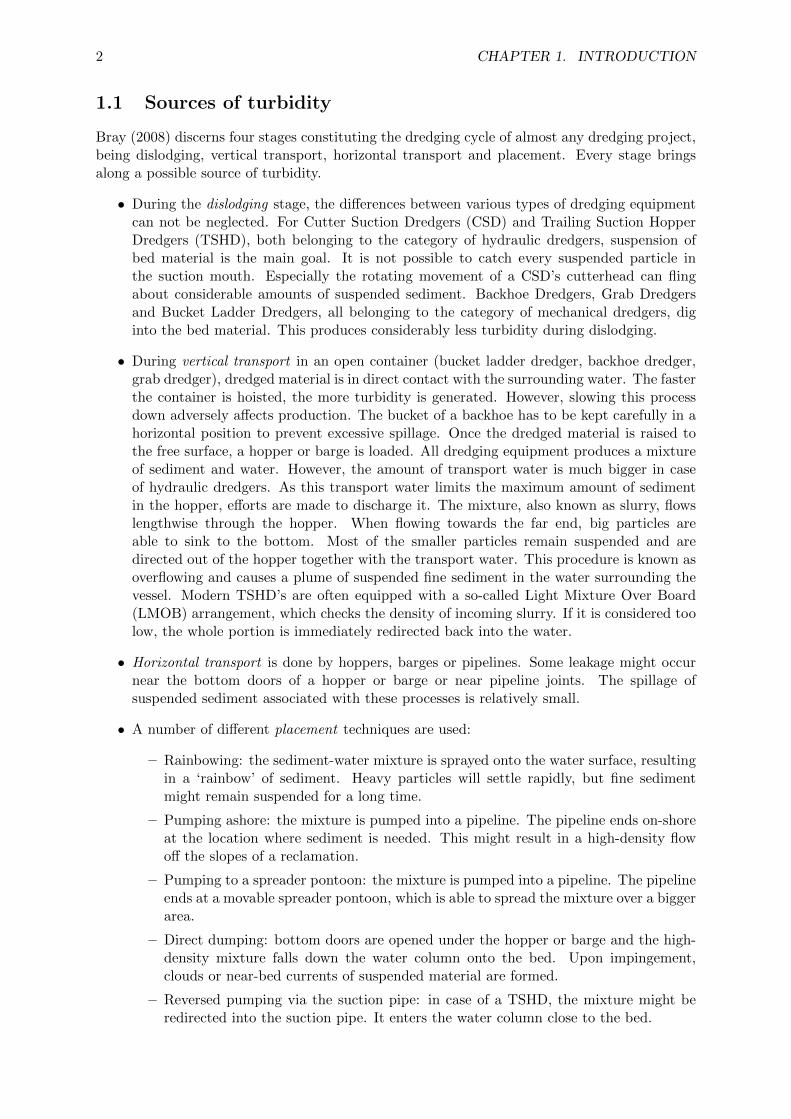
Bray (2008) discerns four stages constituting the dredging cycle of almost any dredging project,being dislodging, vertical transport, horizontal transport and placement. Every stage bringsalong a possible source of turbidity.
• During the dislodging stage, the differences between various types of dredging equipmentcan not be neglected. For Cutter Suction Dredgers (CSD) and Trailing Suction HopperDredgers (TSHD), both belonging to the category of hydraulic dredgers, suspension ofbed material is the main goal. It is not possible to catch every suspended particle inthe suction mouth. Especially the rotating movement of a CSD’s cutterhead can flingabout considerable amounts of suspended sediment. Backhoe Dredgers, Grab Dredgersand Bucket Ladder Dredgers, all belonging to the category of mechanical dredgers, diginto the bed material. This produces considerably less turbidity during dislodging.
• During vertical transport in an open container (bucket ladder dredger, backhoe dredger,grab dredger), dredged material is in direct contact with the surrounding water. The fasterthe container is hoisted, the more turbidity is generated. However, slowing this processdown adversely affects production. The bucket of a backhoe has to be kept carefully in ahorizontal position to prevent excessive spillage. Once the dredged material is raised tothe free surface, a hopper or barge is loaded. All dredging equipment produces a mixtureof sediment and water. However, the amount of transport water is much bigger in caseof hydraulic dredgers. As this transport water limits the maximum amount of sedimentin the hopper, efforts are made to discharge it. The mixture, also known as slurry, flowslengthwise through the hopper. When flowing towards the far end, big particles areable to sink to the bottom. Most of the smaller particles remain suspended and aredirected out of the hopper together with the transport water. This procedure is known asoverflowing and causes a plume of suspended fine sediment in the water surrounding thevessel. Modern TSHD’s are often equipped with a so-called Light Mixture Over Board(LMOB) arrangement, which checks the density of incoming slurry. If it is considered toolow, the whole portion is immediately redirected back into the water.
• Horizontal transport is done by hoppers, barges or pipelines. Some leakage might occurnear the bottom doors of a hopper or barge or near pipeline joints. The spillage ofsuspended sediment associated with these processes is relatively small.
• A number of different placement techniques are used:
– Rainbowing: the sediment-water mixture is sprayed onto the water surface, resultingin a ‘rainbow’ of sediment. Heavy particles will settle rapidly, but fine sedimentmight remain suspended for a long time.
– Pumping ashore: the mixture is pumped into a pipeline. The pipeline ends on-shoreat the location where sediment is needed. This might result in a high-density flowoff the slopes of a reclamation.
– Pumping to a spreader pontoon: the mixture is pumped into a pipeline. The pipelineends at a movable spreader pontoon, which is able to spread the mixture over a biggerarea.
– Direct dumping: bottom doors are opened under the hopper or barge and the high-density mixture falls down the water column onto the bed. Upon impingement,clouds or near-bed currents of suspended material are formed.
– Reversed pumping via the suction pipe: in case of a TSHD, the mixture might beredirected into the suction pipe. It enters the water column close to the bed.

1.2. ENVIRONMENTAL IMPACT 3
The choice depends on the purpose of dredging and some site-specific circumstances. Un-derwater spreading of relocated material occurs due to wave and current conditions anddensity effects. Fine particles remain suspended for long periods of time. The biggestpart of it gets dispersed and does not end up at the intended location. In case of cap-ital dredging, the newly reclaimed land might be eroded by wave and current action orprecipitation runoff. This increases turbidity levels as well.
1.2 Environmental impact
The presence and spreading of suspended sediment concentrations (SSC) does not necessarilyimply negative consequences. Certain dredging and reclamation locations are confronted withrelatively high levels of turbidity by nature. In order to survive, ecosystems adapt themselves tonatural local circumstances (the so-called background conditions). Long periods of exposure toan unnatural level of SSC can result in irreversible impact. Dredging-induced SSC are linked tothe duration of the dredging project, which is usually in the order of months to years. Especiallyin shallow coastal zones vulnerable aquatic flora and fauna are present.
There are five possibly negative effects of SSC for the environment:
• It affects the light transmittance of the water. Typical examples of species vulnerable toshading are fields of sea grass and coral reefs. These species drive complete ecosystemsand are known to recover slowly. A lack of sunlight can lead to irreversible impact.
• Upon settling, a layer of fine sediment is formed on the bed. This can disturb the benthiccommunity to a high degree. Fauna will probably be able to cope with such an event thanbetter flora, since it has a higher mobility.
• It hampers the activities of animals relying on their sight when hunting. To birds especiallythe upper metre of the water column is of importance.
• Suspended sediment has to be kept away from certain water intake structures. Regardlessof their purpose, high SSC will often pose a threat to the underlying facility.
• Turbidity at the free surface has also got an aesthetic effect. Near bathing areas, turbidwater can hamper recreational activities. An additional aesthetic effect, though of lessimportance, is the public opinion. Turbidity always looks like a threat to the environment.This might increase the number of opponents of a certain dredging project, regardless ofthe real environmental damage done.
1.3 Purpose of silt screens
Whenever it is undesirable that fine suspended sediment spreads freely, a choice has to be madebetween different mitigating measures. All mitigating measures can be classified in a spectrumbetween source and receiver. The following measures can be applied according to Bray (2008),ordered from source-based to receiver-based:
• Careful selection of dredging equipment
• Modification of dredging equipment, e.g. application of closed environmental grabs
• Operational measures on board the dredgers, e.g. limiting bucket hoisting speed or over-flow quantities
• Removal of fines from the dredged material, e.g. by means of a settlement pond

4 CHAPTER 1. INTRODUCTION
• Seasonal or tidal restrictions to placement in order to avoid heavy hydrodynamic condi-tions which promote spreading
• Containing or controlling suspended sediment, e.g. by means of a silt screen
It becomes clear that silt screens are applied at the far end of a dredging operation, relativelyclose to possible receivers.
The purpose of all these measures can be defined based on the environmental threats as discussedin section 1.2. Firstly, it has to be avoided that high SSC settles on vulnerable benthic species.Of course this does not mean that suspended sediment has to be prevented from settling atall. It will always do so eventually. Generally, vulnerable species are not located right next tothe screen. Therefore it is a matter of making sure the fine sediment does not get transportedtoo far in high concentrations. Secondly, the light transmittance has to be maintained at anacceptable level. Here the same argument is valid: a vulnerable receptor will not be situatedexactly at the dredging site. High SSC have to be kept close to the silt screen. Finally, a clearand unclouded free surface has to be preserved because of aesthetic reasons. This goal has tobe reached everywhere on the ‘outer side’ of the screen.
Given these different purposes, the effectiveness of silt screens can be defined. Leakage isinextricably linked to the concept of silt screens. In the context of mitigating impact of dredgingoperations, the effectiveness is therefore related to the degree to which the escaping fines arepresented to the environment in a desirable way. In the past, the focus of research into silt screeneffectiveness has always been on comparing SSC, suspended sediment fluxes and turbidity onboth sides of the silt screen (JBF Scientific Corporation, 1978; Yasui et al., 1999; Jin et al.,2003; Bray, 2008; Vu et al., 2010). In this research an attempt is made to derive a more precisedefinition, since the various goals summed up above are not completely covered by the statedparameters. A measure for silt screen effectiveness should include the following aspects:
• The sediment has to settle as quickly as possible once it has past the silt screen. The closerit is to the bed, the shorter the settling time will be. Quantitatively this demand couldbe expressed as the product of a concentration and its distance to the bed. A comparisonof this parameter at both sides of the screen determines whether the screen is effective atall.
• The free surface has to remain clear. Water gets already turbid at very low suspendedsediment concentrations. Effectiveness is related to the position of the limit turbidity inthe water column.
Not all purposes are applicable in a specific situation. Therefore the different aspects thatmake up silt screen effectiveness should be assessed and judged separately. A more elaboratedescription of the parameters which constitute silt screen effectiveness can only be presentedafter having discussed the theoretical part of this research. Section 2.5 continues on this topic.
1.4 Types of silt screens
Silt screens come in different shapes and with different properties, but they are always based onone of two general types. These are the hanging type and the standing type. Both are depictedin figure 1.1.
The hanging type consists of a sheet, mostly constructed from geotextile, that hangs downfrom floats at the free surface. To prevent the entire sheet from floating up, a weight chainis added at the lower side. When pressures on a hanging silt screen get too high, the sheetwill flare and allow the current to flow underneath more easily. The anchorage construction

1.5. CURRENT STATE OF RESEARCH 5
Figure 1.1: The two main types of silt screens. On the left a screen of the hanging type, on theright one of the standing type. In case of reversible flow, the hanging type needs to be anchoredon both sides.
needs to have sufficient clearance. In that way the screen can move along with waves and tides.Anchorage of the bottom edge to avoid flaring induces unacceptably large forces.
In case of the standing type, the sheet is fixed to a heavy beam that lies on the bottom.Floats are attached to the top side of the sheet and pull it towards the free surface. Just likewith the hanging type there is a release mechanism. Overpressure will force the floats to sinkdown and allow water to flow over the screen. A specific failure mechanism related to thistype occurs when settled sediment piles up next to it. The sheet and sinking beam might getpartially buried, which complicates removal of the barrier to a great extent.
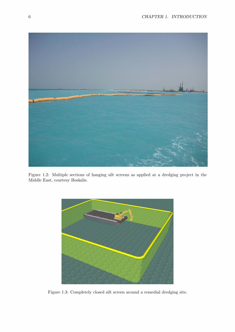
The choice between both types is often made based on operational rather than physicalarguments. Near medium and big sized dredging and reclamation activities, silt screens haveto be relocated regularly to keep up with the actual dredging or dumping location. In case of astanding silt screen, relocation requires quite heavy floating equipment. Therefore contractorsusually prefer hanging silt screens, which can be relocated relatively easy. This research willfocus on hanging silt screens, as those are applied most often and their effectiveness is questionedthe most. Figure 1.2 shows an example of hanging silt screens in dredging practice.
1.5 Current state of research
Due to its big surface area, a silt screen has to withstand large forces. Hence, much effort hasbeen done to optimise silt screens from a mechanical point of view. Investigations regardingstrength by JBF Scientific Corporation (1978) marked the beginning of silt screen research.They also addressed the effectiveness of silt screens based on analytical studies and field mea-surements, but only very few conclusions were drawn on that topic. Field measurement out-comes are influenced by various site-specific conditions. It becomes clear that silt screens areapplied in many different geometries. In these early days, awareness of all possible environmen-tal aspects related to dredging was still fairly low. Silt screens were especially applied aroundremedial dredging works, involving contaminated soils. Generally the size of remedial dredgingsites is small. This enables contractors to apply a completely closed silt screen right next to thedredging site, see figure 1.3. Spreading of suspended sediment close to the dredging equipmentis mostly density-driven. De Wilde (1995) and Yasui et al. (1999) concluded that silt screens in
6 CHAPTER 1. INTRODUCTION
Figure 1.2: Multiple sections of hanging silt screens as applied at a dredging project in theMiddle East, courtesy Boskalis.
Figure 1.3: Completely closed silt screen around a remedial dredging site.

1.6. ENGINEERING PRACTICE 7
closed formation can be a very effective measure. Special attention is paid to the mechanismsleading to turbidity decay. Regarding mechanical strength and stability of silt screens, it isgenerally concluded that silt screens should not be applied in current velocities above 0.5 m/sor wave heights above 0.5 to 1.0 m. It is possible to improve mechanical properties of both siltscreen and anchorage, but costs rapidly increase.
Gradually attention has shifted to the overall environmental impact of turbidity, regardlessof contamination. In this respect, silt screens are applied in many different geometries. Areport by Francingues and Palermo (2005) bundled the conclusions of various researchers intoone engineering guideline. It states that a rigorous examination of silt screen performance is aremaining challenge. In Jin et al. (2003) again a series of field measurements is discussed. Thecomplexity of the measurements poses difficulties trying to extract rigid conclusions. At leastin a number of cases silt screens have proved to be ineffective.
From an academical point of view, research of Vu and Tan (2010) is worth noticing. Itfocuses on the performance of silt screens as a sediment control equipment, which comes veryclose to investigating the effectiveness. More results are still to come, but qualitative resultsof among others laboratory experiments have already been published. They include ParticleImage Velocimetry measurements of a silt screen in a flume.
On the whole, silt screen research is heavily biased towards consideration of strength and stabil-ity during the design stage (Vu and Tan, 2009; Vu et al., 2010). Detailed and rigid conclusionson silt screen performance have not been drawn yet. For that purpose, systematic researchis needed instead of incidental stand-alone field experiments. Nevertheless, the latter will behelpful in relating research outcomes to engineering practice.
1.6 Engineering practice
The actual application of silt screens as a mitigating measure always results from certain reg-ulations limiting free spreading of suspended sediment. These regulations are usually imposedby the local government or permitting authority. In developing countries, where environmentallegislation is often lacking, many project owners or financiers develop regulations themselves.However, biodiversity in a certain region can never be charted completely. Furthermore theresponse of aquatic flora and fauna to turbidity is known only in general terms. As all speciesadapt to their direct environment, the response of the same organism might differ from siteto site. Therefore it is impossible to develop perfectly tailored environmental legislation. Thecommon answer to uncertainties in engineering is found in over-dimensioning. Hence regulatorswill usually aim for strict environmental terms.
Likewise, the exact spreading of turbidity plumes is uncertain. Monitoring campaigns are setto keep track of SSC and turbidity at various locations surrounding a dredging or reclamationsite. Nevertheless, the discrete nature of these measurements and in many cases the impossibilityto perceive sub-surfacial turbidity will never lead to complete certainty regarding exceedance ofSSC limits.
As a result, regulations can not be maintained strictly. So although silt screens are oftenapplied when regulations seem to call for mitigating measures, once deployed their performancebecomes less important. In addition to this, project owners often have unrealistic expectationsof silt screens. They overlook operational consequences and think of silt screens as turbiditycontainers rather than current deflectors. Sometimes project owners even copy environmentaldemands, including the application of silt screens, from one project to another, regardlessof varying conditions. Contractors are confronted with silt screens more often. From theirexperience, they know that silt screen effectiveness is rather doubtful and depends heavily onlocal circumstances. See appendix A for discussion of silt screen effectiveness in a number ofcase studies.

8 CHAPTER 1. INTRODUCTION
Currently, much effort and money is wasted on ineffective applications of silt screens, whereother mitigating measures may have been more effective and cost efficient. Thorough researchinto silt screen effectiveness is beneficial for all parties involved:
• Environmental risks can be reduced by not relying on inappropriate mitigation measures.
• Contractors and clients are able to limit costs by only applying silt screens when they arereally effective regarding local circumstances.
• Regulators are better able to judge whether it is appropriate to demand the applicationof silt screens given their effectiveness in a specific case.
1.7 Research objective
This research will provide increased insight into the most important processes determining siltscreen effectiveness. Based on the results, a design guideline can be constructed, stating underwhich conditions a silt screen is an effective solution. The main research objective is formulatedas follows:
To obtain insight into the most important processes determining transportof suspended sediment in the vicinity of hanging silt screens and to deter-mine the effectiveness of hanging silt screens under varying circumstances.
Both parts of the objective are explicitly limited to hanging silt screens, because both their ap-plication and doubts about their effectiveness are the most widely spread. It will be achievedby addressing the following research questions:
1. To what extent do varying flow velocity, water depth, relative height of the screen, settlingvelocity and upstream SSC profile affect the effectiveness of a hanging silt screen in uniformcross flow?
2. Can basic adjustments to the small-scale design and large-scale application of hanging siltscreens improve their effectiveness?
The first question will result in a sensitivity analysis of the effectiveness with respect to thestated parameters. A design guideline for the application of hanging silt screens in uniform crossflow can be constructed based on this analysis. By relative screen height the ratio of screenheight over water depth is meant.
The second question discusses the possibility to improve silt screens. A couple of promisingadjustments is developed and investigated rather than really striving to optimise silt screens.Both the small-scale design and the large-scale application are taken into account. The formerfocuses on adjustments to the cross-section of a hanging silt screen. For example, perforating thescreen might influence the current pattern in a favourable way. By the latter, the general wayin which silt screens are applied is called into question. For example, it might be advantageousto use hanging silt screens as a horizontal current deflector rather than a vertical one.
The tools used to reach the objective consist of laboratory experiments and numerical mod-els. Their specific application in different parts of this research is closely related to the relevantphysical processes. Therefore the application of these tools is explained in chapter 3.

9
Chapter 2
Theory
Silt screens are surrounded by a couple of different processes, literally as well as figuratively.First of all, the relevant processes regarding the effectiveness of silt screens are identified. Thenthe general flow field in the vicinity of a silt screen is introduced. The third section discussesa couple of basic phenomena related to suspended (fine) sediment, whereas the fourth sectioncovers the specific case of a dredging-induced sediment spill. This chapter concludes with a wayof quantifying the effectiveness of silt screens.
2.1 Key processes
First an inventory of all processes related to hanging silt screens in uniform cross flow is made.After that the processes that are of most importance to this research can be selected.
2.1.1 Inventory
When assessing the effectiveness of a silt screen, insight into the related flow and transportprocesses is paramount. It is known that the spreading of fines can never be stopped completely.Hence two questions arise: which mechanisms are responsible for sediment loss and which agentsactually transport the sediment past the silt screen?
Four sediment loss mechanisms can be identified:
• The most obvious sediment loss mechanism is situated near the bottom. In a horizontalcurrent, continuity forces water to get past the screen. A gap is left open between thebottom and the lower edge of the silt screen. The current is then diverted vertically.Nothing prevents the sediment from flowing along.
• The second mechanism is related to the horizontal plane. A silt screen has got finitedimensions and partly blocks the flow, so the current might also be diverted horizontallyand pass the screen sideways. Engineers will always try to design a silt screen in such away that the dredging plume does not simply end up in that current, but the mechanismcan not be neglected.
• The third sediment loss mechanism is found at the free surface and is not as well-definedas the previous ones. In case of rough flow conditions, water might be splashing or washingover the floats. However, in case of such rough conditions many other and more severeproblems will occur. The construction can not withstand these big forces and will fail.For the sake of completeness, the mechanism is not left out of these initial considerations.
• The fourth and last mechanism is related to the segmentation of a silt screen. One sectionof a silt screen typically has got a width of about 100 m. That is mostly shorter than the

10 CHAPTER 2. THEORY
design width of a complete screen. At the locations where two sections come together,there will not be a sand tight connection. This induces leakage of sediment.
The treatment of the sediment loss mechanisms has already shown a glimpse of the agentsthat actually transport the sediment past the silt screen.
• First of all ‘external’ currents can be named as one of them. In this case ‘external’ meansthat the forcing of the flow has got nothing to do with the presence of a silt screen orsuspended fines. Think for example of tidal or river currents. Eventually every identifiabletransporting or mixing agent, except for ‘true’ diffusion, can be related to the presenceof flow. Nevertheless from here on these external currents are simply indicated as flow.Wind-driven currents belong to that category as well, but their different flow profile hasto be noted.
• The second agent, being waves, eventually also comes down to the generation of flow.However, its specific character makes separate treatment beneficial. With waves wave-induced currents are associated. These are able to affect the spreading of turbidity. Theinteraction between waves and a silt screen may also lead to dynamic processes capableof transporting suspended sediment.
• The third agent is related to a somewhat different forcing mechanism, namely buoyancy.Turbid water obtains a slightly higher density. When it mixes with clear water, thedensity difference starts to drive a current. It goes without saying that fine sediment isthen transported along.
Table 2.1, gives an overview of the relations between sediment loss mechanisms and agentsas named above. A plus sign indicates a weak relation, a double plus sign indicates a strongrelation and a zero indicates no significant relation. The numbers are used to indicate therelations in the remainder of this section.
Table 2.1: Relations between sediment loss mechanisms and agents.
Agents
Flow Waves Buoyancy
Mech
an
ism
s Vertical diversion ++ (1) ++ (2) + (3)
Horizontal diversion ++ (4) 0 (5) 0 (6)
Overwash + (7) 0 (8) 0 (9)
Leakage + (10) + (11) + (12)
1. In case of external currents with a component perpendicular to the silt screen, the screenwill start to act as a flexible baffle. Flow acceleration on the upstream side takes amajor part of the suspended sediment with it. Deceleration and flow separation on thedownstream side lead to a significant amount of turbulent mixing and an upward velocitycomponent. This brings the sediment to a higher position in the water column and delaysthe settling process. Therefore it is an important process regarding the effectiveness ofsilt screens.
2. Wave-induced currents are known to have a narrow boundary layer, which leads to rel-atively high flow velocities near the bottom. The back and forth going character of thecurrent leads, except for a possible residual, theoretically to zero transport. However, thepresence of the silt screen makes a difference. The aforementioned flow separation will

2.1. KEY PROCESSES 11
also take place in case of wave-induced currents underneath the screen. The current pat-tern will not be exactly reversible anymore. This induces a nett transport. Generally siltscreens are not applied in case of waves higher than about 0.5 m, but the related currentsmight still be significant. This becomes clear after a calculation of the order of magnitudeof wave-induced currents near a silt screen. Under assumption of a water depth of 8 m anda 0.5 m swell wave with a period of 10 seconds, the velocity amplitude near the bottomaccording to linear wave theory (e.g. Holthuijsen, 2007) is about 0.26 m/s. This is thesame order of magnitude as the maximum constant flow velocity at which silt screens canbe applied.
3. The increase in density due to suspended sediment concentrations will typically be in theorder of one promille. Nevertheless it will still be able to drive a current. The influencewill probably only be really distinguishable in absence of external flow and waves, but thedensity difference will always contribute to the total flow pattern.
4. Due to the presence of a silt screen, a current will be diverted vertically as well as horizon-tally. The screen’s geometry determines the distribution between those two mechanisms.
5. Wave-induced current does not induce a significant mass transport outside of the surfzone and away from any disturbing factors. Therefore it will not be able to transport finesediment around the side edge of a silt screen.
6. If a part of the suspended fines ends up to the side of the screen, the concentration willbe much lower than in the middle of the screen. Density effects are then negligible.
7. Rough flow conditions might be able to make water wash over the floats. As said before,regular silt screens will fail in such circumstances and will not be applied in first place.
8. Although in practice silt screens are never applied under wave conditions that are ableto send water splashing over the floats, theoretically it might be the case. However, JBFScientific Corporation (1978) proves that virtually no expected wave is able to swamp thefloats.
9. As density currents take place at some distance below the free surface, overwash does notrelate to this agent.
10. A current can find its way past a silt screen through the joint of two sections. When thejoint is well-constructed this will not be a very strong effect.
11. The same can be said about wave-driven current. Due to the presence of the silt screenit is not perfectly reversible, but the narrow open spaces in a joint do not allow for muchflow.
12. Density effects were said to be weak in case of a big gap near the bottom. In case ofa smaller gap that is situated higher in the water column overpressures due to densityeffects are smaller. Therefore their influence is only marginal.
Silt screens are not really preventing the suspended fine sediment from spreading freely. Theyinfluence the way in which suspended sediment is presented to the surroundings. Sediment mayget past the screen, as long as this contributes to quick settling. In principle suspended sedimentis directed towards the bottom when it is transported by the contracting current. This leadsto a shorter settling time. Turbulence and flow recovery downstream of the screen counteractthis process. The intensity of the flow determines whether the silt screen still promotes settling.Figure 2.1 illustrates this schematically. When turbulence intensities are too low for significantturbulent mixing and the settling velocity can withstand the vertical velocity component, sedi-ment will settle. In case sediment is forced to a position lower in the water column, the smaller

12 CHAPTER 2. THEORY
Figure 2.1: Processes regarding flow under a silt screen.
Figure 2.2: Silt screen deformed by a current.
settling time is not the only advantage. Fully developed tidal or river flow is known to have alogarithmic flow profile. Closer to the bottom the ability of the current to transport sedimentis smaller. This will keep turbidity closer to the dredging site.
Two properties of the silt screen itself need to be addressed as well, being flexibility and per-meability. Currents, waves and density differences lead to pressure differences between bothsides of the screen. Eventually that results in deformation of the geotextile. These pressuredifferences will remain more or less constant under stationary conditions. The screen obtains acertain deformed shape and will stay that way until conditions change. Figure 2.2 schematicallyshows the way a silt screen will deform under influence of a current. Due to the deformation, theacceleration zone on the upstream side of the screen becomes more streamlined. This especiallyaffects the current pattern upstream, but also downstream some influence will be noticeable.When the lower side of the silt screen is anchored, the deformation is of course limited withinthe clearance of the anchorage. However, from JBF Scientific Corporation (1978) it is knownthat anchoring the lower edge induces unacceptably large forces on the construction.
Silt screens are mostly made of geotextile. In theory this makes them permeable. However,the structure of the cloth is already very fine to guarantee sediment-tightness. Accumulationof sediment can result in a filter cake and marine growth might deteriorate permeability evenfurther. On the whole it is known from Francingues and Palermo (2005) that water rather flows

2.1. KEY PROCESSES 13
around a silt screen than through it. This appears to be the path of least resistance.
2.1.2 Focus
Analyzing table 2.1, it becomes quite clear which processes are the most important regardinghanging silt screens in uniform cross flow. Vertical diversion due to flow and waves and horizontaldiversion due to flow determine the effectiveness to a large extent. These three processes eachrequire their own approach. All aspects related to vertical diversion happen in a vertical cross-section perpendicular to the silt screen. In modelling terms a 2DV approach suffices in that case.Despite the dimensional similarity, a stationary or quasi-stationary current behaves completelydifferent from wave-induced current. Horizontal flow diversion requires the inclusion of bothhorizontal dimensions. In principle a 2DH approach is appropriate, but the current patternassociated with horizontal diversion might have a significant vertical component.
It is not feasible to include all three processes in this research. The differences that existbetween them call for separate treatment. Wave-induced currents were said not to be per-fectly reversible in the vicinity of a silt screen. Nevertheless the associated effect on suspendedsediment still remains very local. The flow-related sediment loss mechanisms are capable oftransporting sediment further away from the screen. Therefore the basic effectiveness of a siltscreen is determined by these two flow-related processes. It becomes clear that assessing themshould be the starting point of scientific research into the effectiveness of silt screens.
Besides its smaller importance, it is very difficult to investigate wave-induced currents neara silt screen. The flexibility of the screen and the degrees of freedom of the floats facilitate anearly complete transmission of wave energy. Both aspects can not be accounted for in a regularnumerical model. Very complex adjustments would be needed in that case. A physical modelcan represent both flexibility and movability. However, the current pattern of a wave dependsheavily on the pressure distribution. A scale model will not have exactly the same proportionsand properties as a real silt screen. Therefore it is questionable whether the pressure distributioncan be reproduced satisfactory.
Vertical diversion will be studied most extensively, since doubts about silt screen perfor-mance are mostly related to this process. It depends on the specific application whether hori-zontal diversion is likely to happen, whereas vertical diversion will always take place in case ofa hanging silt screen in cross flow.
Now the focus of the second research question will be determined. It consists of two parts,being adjustments to the large-scale application of silt screens and the small-scale design. Asmentioned before, this topic will not be treated exhaustively. It is not aimed to optimise appli-cation and design. Yet they are included, because the tools used in this research offer a uniqueopportunity to study the effects of a number of promising adjustments along the way. Whenconsidering the large-scale application, silt screens are regarded as 2DH solutions influencing thehorizontal velocity field. By small-scale design of silt screens, the cross-section is indicated. Thisis associated to regarding silt screens as a 2DV solution. The adjustments to be included in thisresearch are systematically derived in appendix B. The following adjustments are consideredpromising (the codes stem from the appendix and are re-used later on in this report):
• 1a: Horizontal current diversion by deploying a silt screen obliquely with respect to thecurrent (2DH)
• 1b: Horizontal current diversion by deploying silt screens in a V-shape (2DH)
• 2a: Promote settling due to decreased downstream turbulence by perforating the screen(2DV)
• 2b: Promote settling by extending the silt screen with a flap (2DV)

14 CHAPTER 2. THEORY
Figure 2.3: Basic geometry of 2DV flow under a baffle with all its relevant parameters.
• 3a: Extensive mixing by creating a gap between adjacent sections (2DH)
• 3b: Extensive mixing by creating a diffuser (2DH)
• 5: Halting by catching the plume in between two consecutive screens (2DV)
2.2 Flow-related phenomena
Flow is expected too be the most influential agent to the effectiveness of silt screens. It iscapable of transporting suspended solids either by advection or diffusion. The presence of thescreen leads to a significant increase of turbulence intensity. In this section the theoretical flowfield around a silt screen is discussed, based on research by Vu and Tan (2010) and the simplifiedcase of flow under a baffle. Appendix C contains general theory on turbulent flows (e.g. Pope,2000).
2.2.1 Flow under a baffle
Silt screens can be thought to function as a baffle. Two-dimensional flow under a rigid verticalbaffle is a popular academical case to researchers. A typical layout with its relevant parametersis given in figure 2.3. The mean underflow at the point of maximum contraction U0 is equalto the specific discharge divided by h0. Associated flow profiles still depend on the boundaryconditions. The jet Froude number Fr j = U0/
√gh0 determines whether conditions are sub- or
supercritical underneath the baffle. When Fr j > 1 a free or submerged hydraulic jump occurs,depending on downstream water depth h2 .
In case of a silt screen, upstream and downstream water depth h1 and h2 are approximatelyequal, since silt screens are never applied to regulate large-scale flow characteristics. The rangeof possible jet Froude numbers is computed based on some extreme values. Undisturbed meanflow velocity U varies between 0 and 0.5 m/s and water depth h varies between 2 and 10 m,corresponding with undisturbed Froude numbers of 0 to 0.1. Instead of h0, the dimensionlessrelative baffle height hrel = 1 − h0/h will be used. It varies between 0.25 and 0.75. Figure 2.4shows that for hrel < 0.8 and Fr < 0.1, which is generally the case, flow will stay subcritical.When hrel and Fr are very big, theoretically supercritical flow might occur. However, for thecase of silt screens some remarks have to be made. The screen is flexible, which allows forsignificant pressure transmission. Flow information can therefore not only travel through thenarrow opening underneath the screen, but through the screen itself as well. Hence the realwave celerity in the jet will be bigger than
√gh0. Furthermore, for big values of hrel, significant
flaring will take place. This decreases Fr j . On the whole it can be said that flow underneath a

2.2. FLOW-RELATED PHENOMENA 15
Figure 2.4: Contours of jet Froude number Fr j as a function of undisturbed Froude number Frand relative screen height hrel. The red line indicates Fr j = 1, corresponding to supercriticaljet flow.
Figure 2.5: Basic geometry, parameters and downstream velocity profile of a wall jet (panel a)and a submerged hydraulic jump (panel b).
silt screen will always be subcritical.
Typical flow situations related to silt screens that have been analyzed extensively are the walljet and the submerged hydraulic jump. They are schematically depicted in figure 2.5. Thewall jet is thought to flow into an infinite halfspace and gradually spreads out. Eventually itresults in fully developed wall flow with maximum velocity Ue (Launder and Rodi, 1983). Asubmerged jump might occur in case of a baffle. When conditions in the jet are supercriticaland downstream water depth h2 is higher than the critical depth due to some remote boundarycondition, the hydraulic jump is located right next to the back wall of the baffle (e.g. Long et al.,1990). Both have some resemblance to the academical case of a rigid silt screen. However, thesubmerged jump is only present for supercritical jet flow. In case of an academical wall jet thereis neither a closed boundary at the upstream side of the main flow nor a free surface. Thereforea wall jet will never have a zone of reversed flow. The prominent surface roller present in asubmerged jump is governed by an abrupt change of flow regime, leading to more turbulence.

16 CHAPTER 2. THEORY
Figure 2.6: Velocity decay profile downstream of a baffle for both a free jump and a wall jet.Dimensionless maximum streamwise velocity at dimensionless downstream distance is depicted.
In case of subcritical jet flow and a back wall, reversed flow might be established due to anadverse pressure gradient. Continuity deflects the reversed flow to form a recirculation zone.This current pattern is still associated with a significant amount of velocity shear. Thereforeit will lead to an increase of turbulence. In Wu and Rajaratnam (1995) the wall jet, free jumpand submerged jump are assessed. From a self-similarity analysis of streamwise flow profilesit is concluded that the submerged jump forms the transition between a free jump and a walljet. The velocity decay rate in streamwise direction was found to depend on Fr j and thesubmergence factor S. The latter is equal to (hco − h2)/h2, where hco denotes the subcriticalconjugate depth of the issuing supercritical jet flow. In general, the streamwise velocity decayprofile will be wall jet-like for high values of S and free jump-like for low S. However, for lowvalues of Fr j , the profile stays free jump-like at much higher values of S than for high valuesof Fr j . This relation has been established based on supercritical jets with jet Froude numbersdown to 1.07. That is nearly critical. If the trend continues below Fr j = 1, the velocity decayprofile downstream of a silt screen is expected to be free jump-like. Figure 2.6 shows both typesof profile in dimensionless form as found by Wu and Rajaratnam (1995). um is the maximumvelocity in a vertical profile, x is the distance downstream of the jet opening and L is the valueof x at which um has reduced to half of U0. In a free jump, velocity decay rates are somewhatsmoother than in a wall jet. Horizontal velocity decay corresponds to vertical expansion of thejet layer. The faster the expansion rate, the bigger vertical velocities will be. Hence verticalvelocities are the lowest in a subcritical wall jet with bounded water depth, as is the case for asilt screen.
2.2.2 PIV measurements
Vu and Tan (2010) carried out laboratory experiments regarding silt screens. As a part ofthorough research into silt screen effectiveness, the experiments aimed at investigating the flowfield in the vicinity of a hanging silt screen. Amongst others, Particle Image Velocimetry (PIV)measurements were performed on a silt screen in both vertically fixed and loose configuration.Results of this whole-field measurement technique offer the opportunity to assess the flow ingreat detail. Turbulent structures down to the order of one centimeter can be recognised.The experiments largely confirm theoretical expectations. The time-averaged streamlines are

2.3. SEDIMENT-RELATED PHENOMENA 17
characterised by flow contraction upstream and flow separation including a recirculation zonedownstream of the screen. The process of vortex shedding at the tip of the screen is visualised bysuccessive pictures of the instantaneous flow field, see figure 2.7. These same pictures show thatthe theoretical, smooth recirculation zone is a time-averaged phenomenon. Instantaneously, achaotic collection of turbulent eddies is present. This accounts for severe mixing. Time-averagedstreamlines do not show this behaviour. When the screen is anchored in a vertical position, asmall eddy is visible near the free surface on the upstream side. This eddy is absent when thetip is able to move freely. Apparently the deformed shape of a silt screen is not of very bigimportance, as the flow more or less streamlines itself by creating an upstream eddy.
2.3 Sediment-related phenomena
Eventually, research on silt screen effectiveness comes down to the behaviour of (fine) sedimentaround silt screens. Basic theory on the classification and morphodynamics of fine sedimentis found in appendix D. Before any sediment-related phenomena are discussed, a possiblemisunderstanding has to be eliminated. The term ‘silt screen’ implies that only non-cohesivefine sediment is involved. Nevertheless, silt screens are applied under cohesive conditions aswell. Dredging often takes place in a salty marine environment. Hence cohesive behaviour ofsediment may not be neglected.
In this section, a qualitative assessment of suspended sediment behaviour in the theoreticalflow field of section 2.2 is made, starting with a passive tracer. Step by step more elements areintroduced: first the influence of the settling velocity is addressed and after that the influenceof increased density is included.
2.3.1 Passive tracer in flow across a silt screen
First of all the behaviour of a passive tracer in the flow field of section 2.2 is discussed. Theupper panel of figure 2.8 indicates three regions typically influencing transport of suspendedmaterial in case of flow across a silt screen. The lower panel visualises the behaviour of a passivecloud when subjected to these processes. In region 1 significant acceleration occurs. This bringsalong strong horizontal gradients of the streamwise velocity component. As the cloud reachesthe gap it is compacted vertically by converging streamlines. In streamwise direction particlesare thrust away from pursuing particles, thus dispersing the cloud horizontally. In region 2, thesudden vertical expansion leads to separation, large velocity shear and reversed flow. This isassociated with high turbulence intensities and a corresponding increase in turbulent diffusion.The area of the cloud subjected to vertical mixing has been increased by dispersion in region 1.Particles are entrained into the recirculation zone, but the cloud is also spread out over the fulldepth of the near-bed jet flow. As a result of these diffusive processes, concentrations decreaserapidly. Region 3 is characterised by deceleration and gradual vertical expansion of the mainflow. Dispersion takes place in vertical direction. The cloud was spread vertically over the jetflow, which expands to the full water depth now. Altogether the presence of the silt screen thusincreases mixing effectiveness. A strong decay of concentrations in the main flow is expectedin case of a passive tracer. Initial dispersion facilitates enhanced turbulent diffusion. In figure2.8, concentrations of dissolved matter outside the main cloud were not mentioned. Large-scaleturbulent structures rip off parts of the cloud, which end up in the recirculation zone. Therethey get diffused further. Gradually dissolved matter re-enters the main flow and is advectedaway from the silt screen.
In practice, suspended sediment spoiled at dredging and reclamation sites does not necessar-ily occur as a discrete cloud. It might also be of a continuous nature. This does not change theprocesses described above. The only difference is the simultaneous occurrence of all processes.So while some suspended matter has already entrained into the recirculation zone, another part

18 CHAPTER 2. THEORY
Figure 2.7: Four successive instantaneous flow fields resulting from PIV measurements by Vuand Tan (2010) at t = 17.33 s (a), t = 17.53 s (b), t = 18 s (c) and t = 18.33 s (d).

2.3. SEDIMENT-RELATED PHENOMENA 19
Figure 2.8: Upper panel: Transport processes in different regions of flow across a silt screen.Lower panel: transport of an initial cloud of passive material. Note how a silt screen ‘stretches’the cloud as a result of dispersion, which increases the surface subjected to turbulent diffusion.

20 CHAPTER 2. THEORY
of the plume is just arriving in the jet flow. As a result turbidity levels will often be more orless equal throughout the whole water column, but it is important to be aware of the underlyingprocesses.
2.3.2 Influence of the settling velocity
Now another element is introduced. The previous section discussed suspended sediment as apassive tracer. Now a settling velocity is introduced to account for the effect of gravity on thegrains or flocs. Fine sediment is known to have a small settling velocity. Even in still andshallow water, settling times can be in the order of days. On short timescales and relativelylarge spatial scales, as is the case for flow across a silt screen, suspended fine sediment nearlybehaves as a passive tracer.
Silt screens might be effective in drastically reducing concentrations because of two possible,favourable effects: promoting spreading or settling. The aforementioned considerations regard-ing settling velocity would rule out the latter, being 50% of the whole potential of silt screens.In three situations a silt screen might still promote settling of suspended sediment:
1. Upward current velocities (w) and turbulent shear stresses downstream of the silt screenare small due to very calm flow conditions. Relatively big silt grains in the order of 63mm might still be able to settle.
2. The suspended sediment is cohesive. In salt water flocculation of cohesive sediment will bepromoted. The flocs have an increased settling velocity and are therefore able to withstandupward flow velocities to a larger extent.
3. Concentrations of suspended sediment are high enough to induce density effects. Thedense layer stays close to the bottom. Furthermore, stratification is able to reduce theinfluence of turbulent mixing.
Situation 2 and 3 lead to a substantial increase of ws. However, they only occur in case ofcertain specific circumstances. Section 2.3.3 elaborates on the influence of density effects.
The influence of the settling velocity can be expressed by evaluating the dimensionless parameterws/w. Any dependency of ws on different parameters is left out of consideration here, as thisdependency differs for cohesive and non-cohesive sediment. The vertical flow velocity w dependsapproximately linearly on the horizontal flow velocity u downstream of the silt screen. u in turnvaries with relative screen height hrel and upstream depth-averaged flow velocity U . The relationbetween the average issuing jet velocity U0 and hrel is straightforward when screen deformationis neglected. In that case, U0 is proportional to 1/(1 − hrel). Far downstream of the screen,the logarithmic flow profile is restored and there is no relation anymore between u and hrel.Between the screen and the point where the flow has recovered, the influence of hrel graduallydiminishes. The aforementioned proportionality between u and hrel thus represents an upperlimit of the influence of hrel. Finally, it is readily seen that u is approximately proportionalto the upstream depth-averaged flow velocity U . These proportionalities are summarised andelaborated upon in equation 2.1
ws → wsw∝ ws
w ∝ 1
1− hrel→ ws
w∝ 1− hrel (2.1)
w ∝ U → wsw∝ 1
U
The potential of all three parameters only becomes clear after the range of possible values hasbeen addressed. This is done in table 2.2. The last column is governed by the ratio of maximum

2.3. SEDIMENT-RELATED PHENOMENA 21
and minimum dimensionless settling velocity given the extreme parameter values.
Table 2.2: Potential of relevant parameters to influence the dimensionless settling velocity.
Parameter Proportionality Range Potential
U U−1 0.01− 0.3 m/s 30
hrel 1− hrel 0.25− 0.75 3
ws ws 0.001− 3 mm/s 1000
Given the big potential of ws to influence the dimensionless settling velocity and hence theeffectiveness of silt screens, settling velocities of fine sediment can not be neglected beforehand.Settling velocities of the bigger particles or flocs might well be able to counteract vertical flowvelocities, especially under calm conditions.
2.3.3 Density effects
At sufficiently high SSC, the flow field can no longer be detached from the transport field. Highconcentrations of suspended sediment significantly affect the fluid’s effective density, whichmight give rise to stratification. In that case, the density difference drives a turbidity currentalong the bed. Flow velocities in this dense layer differ largely from the theoretical flow field asderived in section 2.2. Exact concentrations at which stratification comes into play can not befound, but Winterwerp (1999) has identified the following stages for suspended fine sediment:
• Low-concentrated mud suspension is found at concentrations ranging from several 10 - 100mg/l. Density differences do not play a significant role.
• High-concentrated mud suspension (HCMS) has concentrations between several 100 - 1000mg/l. HCMS is transported with the main flow, but it is capable of influencing the fluid’seffective viscosity and therefore interacts with the turbulent flow field.
• Fluid mud occurs at concentrations between a few 10 - 100 g/l. A near-bed layer of densefluid is found. In case of dredging-induced SSC this layer is mobile and forms a turbiditycurrent.
The specific properties of HCMS will not be taken into account here. Its effects are lumpedin the settling velocity, which will be varied over several orders of magnitude throughout thisresearch. The next section will elucidate whether stratification may be expected near a specificdredging site. Here the behaviour of turbidity currents in the vicinity of a silt screen is dis-cussed.
At the interface between two layers of different density and with different flow velocities, ex-change of fluid will take place due to breaking internal waves (Turner, 1973). This process iscalled entrainment. Entrainment leads to a less sharp interface with a smooth vertical densitygradient over some height. The bigger the entrainment rate, the higher this transition betweenboth layers will be. When turbulence is only generated by wall friction, the consequences ofentrainment will be limited. The source of turbulence is located in the near-bottom layer. Asthe density difference tends to damp turbulent fluctuations, suspended transport of entrainedsediment in the upper layer will be negligible. However, silt screens are a source of free turbu-lence, which may lead to significant turbulence and hence turbidity in the upper layer. This isa negative effect of silt screens on stratified SSC.
Computing the intensity of entrainment has been subject to discussion in literature, sincesome time-averaged expression has to be brought up to describe the complex interfacial insta-bilities causing entrainment. The starting point of all these different views is the same. The

22 CHAPTER 2. THEORY
entrainment rate is taken proportional to some characteristic velocity, which is often defined asthe difference in horizontal layer-averaged velocity between both layers. Whether a silt screenmagnifies or reduces this velocity difference will only become clear after numerical simulations,which are presented in chapter 4.
2.4 Spreading of dredging spills
Currents and sediment transport near silt screens can not be regarded completely separatedfrom the source of turbidity. The latter determines the upstream vertical profile of suspendedsediment concentrations. Not only does the position of a suspended particle in the water columndetermine where it will end up downstream of the screen, but high concentrations can also inducedensity effects. Whether a density-driven current occurs, is determined by upstream processes.To start with, sediment spills may be caused by a variety of possible dredging operations, allbringing along their own type of spreading. Furthermore, the influence of density differencesmight change during transport of the suspended sediment. These two aspects are now discussedsuccessively. Finally, the implications for the flow and concentration profiles arriving at the siltscreen are discussed.
2.4.1 Types of dredging spills
The various potential sources of turbidity (see section 1.1 for an overview) all have a different wayof directing sediment into the water column. Genarally silt screens are applied as a mitigatingmeasure near the placement site, near relatively small dredging areas and in case of overflowing.Spreading of turbidity in each of these three cases will be discussed below.
During placement, the released mixture may contain a wide gradation of sediment. The coarsergrains will, as intended, settle onto the bed quickly. Only the finer particles will get transportedout of the dedicated placement area. Below, specific spreading mechanisms of all placementtechniques are listed. All placement methods can be classified by the relative importance ofmixing-dominated spreading and density-driven spreading.
• Rainbowing spreads the discharged material over a large surface. The mixture will mixeasily with the surrounding water. Therefore, density differences are too low to form abuoyant plume. Coarse grains settle quickly and fine particles are transported by mixingprocesses.
• Pumping ashore causes a current of dense material to enter the water column on top ofthe reclamation’s side slope. Given the significant angle of inclination, sediment is likelyto form a turbidity current down the slope.
• Placement by means of a spreader pontoon causes a high-density mixture to enter thewater column near the free surface. When all grains present in the discharge wouldbehave as individual particles, coarse and fine sediment would split immediately as aresult of differential settling. However, the high concentrations of suspended sedimentissuing from the suppletion pipe give rise to mutual influencing of particles. Particlesmight get pulled into the wake of another particle (cloud formation), but they might alsoslow down due to the return current of another particle (Winterwerp, 1999). As a result,only a part of the fine sediment will gradually get washed out of the discharge, leading toturbidity over the full water column. The remaining part is expected to descent rapidlywithin the plume. Upon impingement on the bottom, an axisymmetric turbidity currentwill be created.

2.4. SPREADING OF DREDGING SPILLS 23
• In case of direct disposal through bottom doors, the processes which were presented fora spreader pontoon will occur as well. However, when a hopper is emptied through apipeline, transport water is added to fluidise the sediment. This is not needed for directdisposal, so concentrations will be higher and the processes involved in hindered settlingwill be stronger. More fine sediment is expected to reach the bottom quickly and spreadas a turbidity current.
• Reversed pumping via the suction pipe leads to a near-bed discharge of high-concentratedsuspension. Fine sediment is likely to spread as a turbidity current.
In terms of section 1.1, spreading near small-sized dredging areas involves the stages ofdislodging and vertical transport. Silt screens near dredging sites are only considered cost-effective when the area is small. This is often the case when working with mechanical dredgers.Both dislodging and vertical transport in an open container will dispose low concentrations ofsuspended sediment throughout the water column. Hence, buoyancy will most likely not playa role.
Overflowing induces a negatively buoyant jet of suspended sediment, issuing at the freesurface. The overflow plume solely contains fine particles, as disposing fines is the main purposeof overflowing. Depending on case-specific circumstances, the jet flow either sinks down tothe bottom and forms an axisymmetric turbidity current upon impingement or mixes with thesurrounding water before reaching the bed.
In summary, all dredging spills can be classified as one of the following types:
• A diffusive spill, being advected and diffused by ambient flow.
• A near-bed discharge of negative buoyancy.
• A near-surface discharge of negative buoyancy at some distance from any closed boundary.
• A near-surface discharge on top of a slope.
Based on these types, the diagram of figure 2.9 can be constructed. It shows all possible waysa dredging spill can develop into the upstream boundary condition arriving at a silt screen. Inthe diagram, at two positions a buoyancy criterion is mentioned. Further development of thespill depends on evaluation of this criterion, which is elaborated upon in the next section.
2.4.2 Buoyancy criterion
In dredging plume research two different scopes are distinguished, being near-field and far-field. Near-field spreading is typically associated with the density-driven (also referred to asdynamic) development of a plume directly upon release of sediment particles into the watercolumn. The large-scale, mixing-dominated (passive) spreading of suspended sediment belongsto the far-field. Silt screens are often applied at the edge of near-field and far-field, which isthe reason why two different types of upstream boundary condition were assessed in section2.3. The buoyancy criterion mentioned in figure 2.9 differentiates between dynamic or passivepropagation. First, the general form of this criterion is introduced. Then, this general formis applied to the specific cases of near-surface discharge, a propagating turbidity current anddischarge on top of a slope.
The criterion we are looking for should evaluate the relative importance of buoyancy-promotingand buoyancy-destroying forces. The Richardson number expresses this ratio (e.g. Turner, 1973)and can be used as a criterion in this research. In literature, different forms of the Richardson

24 CHAPTER 2. THEORY
Figure 2.9: Diagram showing the possible developments from dredging spill to upstream bound-ary condition near a silt screen.
number are encountered. The most fundamental form is generally referred to as the gradientRichardson number Ri, see equation 2.2.
Ri =−g ∂ρ∂zρ(∂u∂z )2
(2.2)
In most cases, Ri can be simplified. When dealing with steady flow, adhering to the Boussinesqand hydrostatic assumptions, the type of flow can be classified by means of the bulk Richardsonnumber Ri0, which is defined by equation 2.3.
Ri0 =g′LU2
=
ρ′
ρ0gLU2
(2.3)
Here, g′ denotes the reduced gravitational constant, ρ′ is the density difference governing thespecific flow situation and ρ0 is the reference density which characterises the ambient fluid. Thecharacteristic length- and velocity-scales are derived from the boundary conditions.
Uniform transitional values of Ri and Ri0 cannot be given. For Ri, analytical analysisproves that the transitional value depends on the wave-number(s) of instabilities at the density-interface and the presence of a rigid boundary (Turner, 1973). Regardless of these parameters,the analytical upper limit of the transitional value is 0.25. When Ri is higher than 0.25,buoyancy dominates mixing and stratification is stable. However, counter examples of initiallyturbulent flows remaining turbulent above Ri = 0.25 have been found. When using Ri0, thedefinition of L and U are subject to debate, which obstructs the use of a general transitionalvalue. Mostly, transitional values are derived from case-specific research. A literature reviewregarding the aforementioned types of dredging spills will be presented in the remainder of thissection.
Near-surfacial discharges are a well-studied topic within the field of overflow plume research.Basic theory on plumes is found in e.g. Turner (1973) and Fischer et al. (1979). Field ob-servations of physical processes in actual dredging plumes were reported in a qualitative sense

2.4. SPREADING OF DREDGING SPILLS 25
Figure 2.10: Characteristic pictures of both types of overflow plume spreading: mixing (leftpicture) and density-driven (right picture), Boot (2000).
Figure 2.11: Classification of near-field overflow plume spreading (Winterwerp, 2002). Spreadingis either mixing-dominated or density-driven, depending on a combination of the bulk Richard-son number (horizontal axis) and a velocity ratio (vertical axis).
by Thevenot et al. (1992). Van der Salm (1998) produced the first of a still ongoing series ofscientific reports on the spreading of overflow plumes. He addressed near-field as well as far-fieldprocesses and identified many possibilities for further research. Boot (2000) mainly investigatedthe transition between mixing-dominated and density-driven spreading of overflow plumes. Hisresults in this field were recapitulated by Winterwerp (2002). Figure 2.10 shows examples ofmixing-dominated (left picture) and density-driven (right picture) spreading. They discernedbetween both types of spreading based on the bulk Richardson number and the ratio betweeninitial vertical velocity of the plume and ambient flow velocity (ζ), see equation 2.4.
Ri0 =g′Dp
W 2(2.4a)
ζ =U
W(2.4b)
Dp denotes the overflow pipe diameter, which equals the initial plume diameter, W is thevertical outflow velocity and U is the ambient horizontal depth-averaged flow velocity. Bootand Winterwerp caught their results in a diagram, which is shown in figure 2.11.

26 CHAPTER 2. THEORY
Figure 2.12: Extension of overflow plume classification by De Wit (2010). The contours indi-cate the transition between mixing-dominated and density-driven spreading for different waterdepths. The water depth is expressed as a multiple of the overflow pipe diameter Dp.
During the actual experiments, which were carried out by Boot, the water depth was keptconstant at 8 times the initial overflow plume width. The type of spreading was determinedright before suspended sediment reached the bottom. De Wit (2010) elaborated on this bycarrying out numerical model runs with infinite water depth. The depth at which spreading ofdifferent overflow plumes shifted from initially density-driven towards mixing was documentedfor plumes of varying Ri0. De Wit extended the diagram of figure 2.11 and added transitiondepth contours, see figure 2.12. Within the scope of boundary conditions for silt screens,especially the horizontal transition distance is a parameter of interest. Generally, interactionbetween plume and bed will occur prior to arrival at the silt screen. This interferes with theconcept of transitional depth as investigated by De Wit.
When a density-driven plume impinges on the bed, its momentum starts to drive a radialturbidity current. Its initial height can be derived from a mass balance. Let Bb be the plumewidth prior to impingement, Wb the associated downward mean plume velocity, Uf the hori-zontal velocity of the turbidity current’s front right after impingement and hf the height of thisfront. Assuming that within the impingement zone sediment concentrations remain constant,the mass balance is given by equation 2.5.
1
4πB2
bWb = 2πBbhfUf (2.5)
Horizontal front velocity Uf is related to hf according to equation 2.6, where Fr is the Froudenumber (Bonnecaze et al., 1993). This depends on the ratio of hf over total water depth h.
Uf = Fr√g′hf (2.6)
Fr = 1.19 for 0 <hfh≤ 0.075
Fr = 0.5(hfh
)−13 for 0.075 <
hfh< 1
After elimination of Uf from equation 2.5 by means of equation 2.6, the initial height can becalculated iteratively. Further propagation of a radial turbidity current will be discussed below,together with the associated buoyancy criterion.

2.4. SPREADING OF DREDGING SPILLS 27
A remark has to be made regarding dynamic plumes. Even a dynamic plume will causesediment to mix with ambient water. During the descent of a density-driven plume, somematerial near the plume’s edge is removed by ambient currents. This process, commonly knownas ‘stripping’, was qualitatively described by Thevenot et al. (1992). Based on literature study,Van der Salm (1998) states that about 3 to 5% of all plume material is stripped. Spreading ofthis stripped material is mixing-dominated due to its low concentrations. This leads to turbiditythroughout the whole water column.
In case of a propagating turbidity current, whether or not radial, a characteristic length andvelocity scale are readily found in the height of the current and its horizontal velocity. This isexpressed by equation 2.7.
Ri0 =g′htU2t
(2.7)
According to Turner (1973), transitional values for Ri0 are found between 0.1 and 0.3. Althoughthe buoyancy criterion is straightforward, it remains very difficult to calculate the height andpropagation velocity as a function of place and time for any turbidity current (Bonnecaze et al.,1993). The processes of bed-current interaction and entrainment of ambient water are difficultto parameterise. Non-continuous or radial turbidity currents and ambient currents, as is oftenthe case in dredging practice, add up to that complexity (Bonnecaze et al., 1995; Hallworthet al., 1998). Therefore, it is unavoidable to apply numerical model simulations when thedevelopment of turbidity currents has to be predicted. To this end, yet to be published TASSsoftware (Spearman et al., 2011) might be of great help.
Finally, discharges on top of a slope are discussed. A bottom slope adds kinetic energy to apropagating turbidity current, but it also reduces the component of gravity perpendicular tothe density interface. The former increases the denominator of Ri0, whereas the latter decreasesits numerator. Therefore, downslope turbidity currents will be less stable and mix more easilywith ambient water. Ri0 is defined by equation 2.8 for this case (Turner, 1973). The bottomslope is denoted by φ.
Ri0 =g′ cosφht
U2t
(2.8)
The transition to mixing behaviour of turbidity currents along an incline has not been studiedthoroughly. Turner (1973), Simpson (1987) and Noh and Fernando (1991) only discuss theinitial or steady phase of turbidity current development. Nevertheless, it is expected that atransition to mixing behaviour will not be achieved in dredging practice, as side slopes of areclamation area are of restricted length. After having descended to a more horizontal part ofthe bed, the turbidity current can again be analysed by means of numerical simulation.
2.4.3 Concentration profile
One goal of the preceding considerations in this section is to determine the vertical concentrationprofile upstream of a silt screen. It is evident that the upstream concentration profile influencessilt screen effectiveness to a great extent, as the transport capacity of the flow differs in space.
Concentration profiles may take any possible shape, depending completely on the boundaryconditions. This research focuses mainly on passive concentrations, as silt screens in cross floware usually intended to mitigate the passive part of a dredging spill. If the source of suspendedsediment is located far upstream and the flow is given enough time to redistribute concentrations,an equilibrium profile will arise. When this is the case, there exists a balance between the upwardsediment flux through bed erosion and turbulent diffusion and the downward flux throughsettling and deposition. For non-cohesive sediment, erosion and deposition fluxes remain more

28 CHAPTER 2. THEORY
Figure 2.13: Empirical equilibrium concentration profile for cohesive sediment. The profile hasonly been verified for ensemble averaged data.
or less constant in stationary flow conditions. Provided that hindered settling does not play arole, this gives rise to the well-known Rouse profile.
In case of cohesive sediment, settling velocities depend on the concentration and thereforechange with depth. Furthermore settling velocities are generally much smaller, which leads toa more uniform vertical distribution and a bigger dependency on flow conditions. The lattermakes it difficult to predict a cohesive sediment concentration profile in a specific situation.Only through ensemble averaging it is possible to fit a parameterised profile to empirical data(Whitehouse et al., 2000). Equation 2.9 shows a dimensionless form of this empirical profile.
C
C0=(
1 +Bz
h
)− 1m
(2.9)
with B =mws50b0.0025U
ws50b = kCm0
Here, C0 is the near-bed suspended sediment mass concentration and the coefficient m is thesame as the one in the simplified relation for cohesive settling velocity (equation D.4). Figure2.13 shows two examples of this concentration profile for B = 4.5 and B = 12.
As this empirical equilibrium profile can only be found by means of ensemble averaging, itdoes not provide much information about individual cases. Apart from that, the concentrationprofile arriving upstream of a silt screen will rarely be in equilibrium. It will often depend on acombination of the spill type and local flow conditions. Therefore the upstream concentrationprofile will have to be varied throughout this research. Typical, schematised profiles will beused to that purpose.
2.5 Quantification of silt screen effectiveness
In order to judge any case study or model outcome in terms of silt screen effectiveness, appro-priate definitions are necessary. A new approach on the quantification of silt screen effectivenesswas already proposed in chapter 1. Effectiveness was said to depend on two parameters, being

2.5. QUANTIFICATION OF SILT SCREEN EFFECTIVENESS 29
(1) the product of (time-averaged) SSC and z-coordinate and (2) the vertical position of thevisible turbidity limit in the water column. The former can be determined from the simulationresults straightforwardly. In the remainder of this section the appropriate relation between Cand z will be elaborated upon. The lack of an exact relation between turbidity and SSC impedescomputation of the latter. Many different attempts of researchers to establish this relationshiphave resulted in so many different equations. As the product of concentration and z-coordinateassigns the highest weight to near-surface concentrations, the special disadvantage of surfacialturbidity is still incorporated indirectly.
The aforementioned product of C and z can be regarded as a measure constituting environmentalimpact potential. Here it is investigated whether this is a correct definition. The environmentalimpact of SSC can be addressed in four different ways, see table 2.3.
Table 2.3: Different views at the environmental impact potential of SSC.
Environmental impact
Shading Burial
Scie
nti
fic
field P
hysi
cs
• Absorption of light
• Scatter
• Settling
• Range of attack
Ecolo
gy
• Stress-level of flora &fauna
• Stress-level of flora &fauna
Shading and burial of benthic species are the two main categories of environmental impact(Bray, 2008). For both aspects, two stages can be recognised in determining the impact of SSCon the environment. The presence of sediment particles in the water column invokes severalphysical processes, which in turn can be translated to environmental impact by means of eco-logical arguments.
The aspect of shading will be treated first. As light travels through a medium, its electro-magnetic energy gradually gets absorbed. This is represented by the Lambert-Beer law, whichprescribes the relative intensity (percentage of incoming intensity I0, also called transmissivity)of a light beam as a function of the distance travelled `. For liquids, the law is usually presentedas in equation 2.10.
I
I0= 10−a` (2.10)
Here, I is the intensity after a distance ` and a is the absorption coefficient. The presenceof dissolved matter can be accounted for by adjusting a. The original form of the Lambert-Beer law only holds for monochromatic light (consisting of one single wavelength) with parallelrays in non-turbid waters. This excludes application to natural waters, as sunlight is neithermonochromatic nor parallel and suspended particles in the water create turbidity. The lightattenuating effect of suspended particles lies in the fact that they reflect light beams hence andforth, which is usually indicated as scatter. By doing so, the distance a light beam has to travelin order to reach a certain depth is extended. Hence more energy gets absorbed over each unitof depth, leading to a lower transmissivity. Kirk (1977) showed that the attenuation of light in

30 CHAPTER 2. THEORY
natural waters may simply be represented by a relation similar to the Lambert-Beer law, butwith a much higher absorption coefficient which increases linearly with SSC.
The conversion of light intensity or transmissivity to environmental impact is much harder toestablish. Ecology is not an exact science. It was briefly noted in chapter 1 that the response ofspecies to shading and burial differs from site to site, depending on local background conditions.Nevertheless, species undergo stress from turbidity levels that have risen above the backgroundlevel. Erftemeijer et al. (2012) admit that there is still a rather poor understanding of therelationship between sediment stress and the response of most corals. Following a literaturereview involving 90 case studies, they have categorised corals of different sensitivity accordingto the occurring suspended sediment concentrations and the observed impact. This has resultedin the upper panel of figure 2.14. It shows over which range of SSC a certain impact has beenfound given the coral’s sensitivity to shading. Erftemeijer et al. (2012) distinguish the followingcategories of impact:
• No effect
• Minor sub-lethal effects (e.g. reduced growth, mucus production1)
• Major sub-lethal effects (e.g. bleaching2, tissue damage)
• Minor lethal effects (partial mortality)
• Major lethal effects (mass mortality)
The upper panel of figure 2.14 shows that the environmental impact aggravates more or less lin-early with SSC given a certain sensitivity. This conclusion only holds for corals, but comparablestudies on different species are scarce. For example, a similar literature review for sea grassmeadows by Erftemeijer and Robin Lewis (2006) contains no details on the relation betweensub-lethal effects and SSC. Furthermore, corals are one of the main reasons why the applicationof silt screens is demanded near dredging projects. Hence the use of a linear relation betweenthe to be defined environmental impact potential and C is considered justified for shading.
Burial was named as the second hazardous impact of SSC on the environment. In physicalterms, the amount of sedimentation depends on the near-bed vertical flux of suspended sed-iment. The higher a sediment particle is located in the water column, the longer its settlingtime will be. A longer settling time in turn leads to a larger horizontal distance over whichthe particle is expected to be advected by the current. The characteristic settling distance xs(‘range of attack’) can be defined following equation 2.11.
xs =Uz
ws(2.11)
The amount of sedimentation at distance xs downstream of the reference location will be pro-portional to Cxs. As U and ws are background parameters which also hold when a silt screenis absent, they can be left out of consideration. Hence the product of C and z serves as anappropriate measure for the extent of sedimentation.
The aforementioned research by Erftemeijer et al. (2012) also takes into account the haz-ardous effects to corals of burial. The lower panel of figure 2.14 summarises the results of 102
1Many corals produce a certain amount of mucus. Under sediment stress the production of mucus increases.As a result, the coral consumes more energy than it produces. High SSC or prolonged shading exhausts the coraland may have lethal effects.
2Many corals have a symbiotic relationship with the unicellular zooxanthellae, which account for the colouringof corals. Under sediment stress zooxanthellae may be expelled by the coral, resulting in a colourless appearance.As this bleaching process develops, it becomes increasingly unlikely that the symbiosis is able to recover and thecoral eventually faces lethal effects.

2.5. QUANTIFICATION OF SILT SCREEN EFFECTIVENESS 31
Figure 2.14: Impact of shading (upper panel) and burial (lower panel) for coral species of varyingsensitivity. Modified after Erftemeijer et al. (2012).

32 CHAPTER 2. THEORY
Figure 2.15: Development of the environmental impact potential. The lower panels representthe values of C∗z∗ of the corresponding concentration profiles in the upper panels. Integrationover z∗ leads to P , which is stated above each lower panel.
case studies involving burial of corals. Again, it can be argued that the relation between thesedimentation rate and the environmental impact has an approximately linear character. Com-bined with the physical aspects treated above, this again advocates the use of Cz to define theenvironmental impact potential. The fact that (mobile) benthic fauna are better able to dealwith burial than flora justifies the limitation of this research to corals.
For both shading and burial, a linear relationship was proved to be appropriate. The physicalarguments presented for burial are of special importance, as quick settling is also beneficialregarding shading. The environmental impact potential P is now defined according to equa-tion 2.12. z and C will be made dimensionless by means of undisturbed water depth h andthe maximum upstream concentration Cmax respectively. Through integration over z∗, theenvironmental impact potential only remains a function of downstream distance x.
P (x) =
∫ 1
0z∗C∗ dz∗ (2.12)
with z∗ =z
h
C∗ =C(x, z)
Cmax
To illustrate the behaviour of P , the value of C∗z∗ as a function of z∗ is computed for threeschematic concentration profiles. The result is displayed in figure 2.15. The large contributionof near-surfacial turbidity to the impact potential is clearly shown.
The last step in parameterising silt screen effectiveness consists of converting P to a mea-sure which expresses the actual effectiveness. In order to maximise tangibility and compliancewith literature, it is favourable to express the effectiveness E as an impact reduction percentageachieved by the screen. This can be done in two ways: either by comparing a downstreamvalue P (x) with the value Pin belonging to the issuing concentration profile or by comparing adownstream value P (x) with the value Pref (x) obtained at the same downstream distance ina reference situation without a silt screen. The former percentage will be referred to as Ein,

2.5. QUANTIFICATION OF SILT SCREEN EFFECTIVENESS 33
whereas the latter will be denoted as Eref . To avoid infinitely high percentages, Eref is madedimensionless with Pin. These relations are expressed by equation 2.13.
Ein(x) =
(1− P (x)
Pin
)· 100% (2.13)
Eref (x) =Pref (x)− P (x)
Pin· 100%

34 CHAPTER 2. THEORY

35
Chapter 3
Modelling
The research objective and the focus have been determined and all relevant physical processeswere studied in chapter 2. Now it can be specified how insight into the effectiveness of siltscreens will be obtained given the general focus.
The first research question is applicable to both aspects of the general focus. For both horizontaland vertical diversion the effectiveness depends on a combination of flow velocity, water depth,relative screen height and sediment size. However, in present-day applications, silt screens arealways intended to divert the suspended sediment vertically instead of horizontally. Therefore,determining the limiting dimensions for directing the sediment-laden flow to the screen will bethe purpose of the study into horizontal diversion. Therefore, the ratio between the amountof water flowing under the screen and the amount of water passing the screen laterally undervarying width and height of the screen, water depth and flow velocity will be checked. A 2DHmodel contains all the required features to study this process. In a model based on the shallowwater equations, the silt screen will be represented as a baffle by applying a discharge relationat a series of internal cell boundaries.
Vertical diversion can be investigated in a 2DV approach. The associated flow field is knownto be very turbulent. In a numerical model, turbulence can be schematised in various ways.The possibilities range from a constant turbulent viscosity to more sophisticated solutions suchas Large Eddy Simulation (LES). Nevertheless it still remains a numerical representation. In aphysical model turbulence is present by nature, but the length scales are much smaller than inreality. This limits the size of turbulent structures. When both a numerical and a physical modelare applied, the results of the numerical model can be validated by means of the experimentaldata. Figure 3.1 visualises the investigated relations between model scale and model nature.Modelling at three different levels should lead to reliable conclusions regarding the fourth level.
The modelling activities carried out in the scope of this research can thus be divided into threeparts: laboratory experiments, a 2DV numerical model and a 2DH numerical model. Thedifferent goals per activity are defined below.
The purpose of the laboratory experiments consists of the following aspects:
• The prime purpose is obtaining validation data for the numerical model. High-frequencymeasurements of local velocities at regular spatial intervals provide data to compare time-averaged velocity profiles and turbulence parameters.
• Furthermore, observing the spreading of dye provides qualitative information on both theinstantaneous and the time-averaged flow field. This information is used to verify thenumerical model. All dye injections are captured on video.

36 CHAPTER 3. MODELLING
Figure 3.1: Relations between model scale and model nature concerning the 2DV modellingpart.
• The final aspect is investigating the effect of a number of promising adjustments to the siltscreen. The laboratory experiments are only suitable for the 2DV adjustments: perforationof the screen (adjustment 2a), extending the screen with a flap (2b) and applying anadditional silt screen downstream of the first one (5). The investigation consists of detailedvelocity measurements and observing the spreading of dye.
The specific goals of the 2DV numerical modelling activities are listed below:
• The main part of the 2DV numerical model consists of quantifying the effectiveness ofhanging silt screens under varying flow velocity, water depth, relative screen height, settlingvelocity and upstream SSC profile.
• The 2DV numerical model will also be used to investigate the effect of a number of promis-ing adjustments to the hanging silt screen. Only applying an additional silt screen (5) isfeasible in the applied numerical model.
Finally, the 2DH numerical model aims at the following goals:
• The model is used to determine the influence of flow velocity, water depth, relative screenheight and relative screen width on the distribution of vertically and horizontally divergeddischarges.
• By also varying the angle of incidence, it is possible to assess the screen’s ability to act asa current deflector, which corresponds to adjustment 1a and 1b.
The two numerical codes used for this research are described in appendix F. The academicalDflow3D code will be used for the 2DV approach, whereas the more commercial FINEL2D codewill be used for the 2DH approach.

37
Chapter 4
Vertical diversion
The most important processes determining silt screen effectiveness were said to be vertical andhorizontal diversion. This chapter presents investigations into the former. Results have beenobtained by means of numerical as well as physical modelling. Both have constituted their ownset of valuable observations, but the physical model tests mainly serve as validation data tothe numerical model. Section 4.1 discusses the laboratory experiments. After explaining theexperimental set-up and the different measurement scenario’s, the results are presented. Theseresults already give rise to some considerations regarding the flow field. Suspended sedimenttransport is added in section 4.2, which addresses the numerical model simulations. Successively,the model set-up, validation by means of the laboratory data, the simulation scenario’s and thesimulation results are presented. The section will end with a self-similarity analysis of the flowfield.
4.1 Physical model
A silt screen scale model has been placed in a flume at the Fluid Mechanics Laboratory of theDelft University of Technology. Section 4.1.1 deals with the experimental set-up, the actualseries of experiments is discussed in section 4.1.2 and the results are presented in section 4.1.3.
4.1.1 Set-up
The experiments are conducted in a laboratory flume of 14 m length, 40 cm width and atmaximum 35 cm depth. It is schematically depicted in figure 4.1. Discharge and water depth
Figure 4.1: The experimental set-up used for this research consists of a long flume of 14 mlength, 40 cm width and at maximum 35 cm depth.

38 CHAPTER 4. VERTICAL DIVERSION
Figure 4.2: The silt screen scale model as applied in the flume.
are controlled by a valve in the supply pipe and a weir at the downstream end of the flume.The construction of the silt screen scale model is shown in figure 4.2. The upper bar is made ofrigid foam, so as to clamp the bar in between the flume’s side walls. The screen itself consistsof a cloth. Synthetic material might guarantee complete water tightness, but its mechanicalproperties can not be scaled correctly. A flexible cloth has proved to be practically water tightand behaves more like a real, large-scale silt screen. The weight chain of a real silt screen isaccounted for by a metal rod.
The following measuring instruments are used:
• Measurements of local velocities are made by means of Laser Doppler Anemometry (LDA)with a sampling rate of 500Hz. This leads to very detailed measurements of the turbulentfluctuations. The operating principles of LDA are explained in appendix E. Figure 4.3shows the locations in the flow where velocity timeseries will be collected.
• The discharge is measured by means of a flow meter and a Rehbock weir.
• Water depths at various locations are measured by means of a point gauge.
• A videocamera serves to capture all dye injections on video, so that they can be studiedextensively.
Furthermore the deformed shape of the screen is documented in order to use real deformationsin the numerical model.
4.1.2 Scenarios
A series of different conditions is applied to the experimental setup described above. Eachexperiment is characterised by a unique combination of flow parameters, silt screen geometryand measurements.
Determination of the possible flow parameters is done by scaling a field situation down to flume

4.1. PHYSICAL MODEL 39
Figure 4.3: The blue markers show the locations where velocity timeseries will be collectedby means of LDA. They form 6 profiles of 19 measurements each. A hypothetical position ofthe silt screen is indicated in black. Its lower edge serves as reference point for the horizontalcoordinates.
dimensions. In principle, both the Froude number Fr and the Reynolds number Re of thelaboratory flow should equal Fr and Re of the field situation. By doing so, uniformity of theinfluence of inertia and uniformity of the turbulence properties are guaranteed. However, Reis proportional to the water depth, whereas Fr is inversely proportional to the square-root ofthe water depth. Adhering to both numbers is therefore impossible. Changing Fr leads tounacceptably deformed flow situations and has to be avoided. Changing Re is less rigorous,as long as the flow remains well inside the turbulent regime (Re � 3000). There is no strictrule prescribing the lower limit for Re, since the sensitivity of measurements to the Reynoldsnumber varies from case to case. The flow downstream of a silt screen is obviously dominated byturbulent structures originating from flow separation. On the one hand, scaling can be said tohave a very disadvantageous effect. Re is changed, although turbulence plays an important rolein this specific research. On the other hand, the presence of the screen significantly increasesturbulence intensities, which is not accounted for by Re. This might prevent the flow fromswitching incidentally to laminar conditions. A comparison of numerical model runs at bothscales offers more certainty about the influence of Re.
Three different field scenarios will be scaled down to laboratory dimensions. These scenar-ios are chosen so as to cover the whole range of flow parameters at which silt screens may beapplied. They are listed in table 4.1 and are coded from 1 to 3. Subscript F denotes ‘Field’,whereas subscript L denotes ‘Laboratory’.
Table 4.1: Three combinations of flow parameters that are scaled down to laboratory dimensions.
1 2 3
UF [m/s] 0.2 0.3 0.5
dF [m] 5 5 5
ReF [-] 9.1 · 105 1.4 · 106 2.3 · 106
FrF [-] 0.029 0.043 0.071
FrL [-] 0.029 0.043 0.071
dL [m] 0.35 0.35 0.35
UL [m/s] 0.053 0.079 0.1323
ReL [m] 1.7 · 104 2.5 · 104 4.2 · 104
Furthermore, seven different types of silt screens are used throughout the experiments. Thefirst two types, being A and B, are regular silt screens with different relative screen heights. All

40 CHAPTER 4. VERTICAL DIVERSION
other types are used to investigate the adjustments as discussed previously. The screen typesare coded from A to G, see table 4.2.
Table 4.2: Different types of silt screen used during the experiments with their respective code.
A Regular screen, hrel = 0.5
B Regular screen, hrel = 0.75
C Moderately perforated screen, hrel = 0.75
D Heavily perforated screen, hrel = 0.75
E Screen extended with a flap, hrel = 0.5
F Screen with 1 additional weight chain, extended with a flap, hrel = 0.75
G 2 screens after another, hrel = 0.75
Screen A and B are investigated under all three flow conditions (experiments 1A, 1B, 2A,2B, 3A and 3B). All adjustments are investigated under flow condition 2 (experiments 2C, 2D,2E, 2F and 2G). Experiment 1B, 3A and 3B have an LDA sampling duration of 100 seconds.As this does not lead to satisfactory convergence after time-averaging, experiment 1A, 2A and2B have a sampling duration of 200 seconds.
The deformation of a silt screen is governed by the hydraulic load and the weighting alongthe bottom edge of the screen. The weighting of the scale model should be such that itsdeformations resemble those of the respective field scenario. However, field measurements ofsilt screen deformations are not available. Efforts to compute the shape of a screen in uniformcurrent by means of a simplified model have not proved to be of any use. Finally a weightingof about 1.24 kg/m has been chosen in case of the A and B experiments, since this leads to arealistic order of magnitude of deformations.
4.1.3 Results of laboratory experiments
This section will present the results as obtained from the laboratory experiments. The effec-tiveness of silt screens can only be determined after transport processes have been investigatedwith the numerical model. However, the laboratory results are used to describe the turbulentflow field of flow being diverted vertically by a silt screen.
The results of experiment 2A are shown as an example. Any observation mentioned hereafteris supported by the other laboratory runs. Figure 4.4 shows time-averaged flow velocities. Rawdata of time-averaged vertical velocity w all show the same constant deviation of +0.01 m/swith respect to the expected velocity field (near the bottom and the free surface, w shouldequal zero). Hence all data regarding w have been corrected manually. The theoretical flowfield as described in chapter 2 clearly applies to the experiments. Right downstream of thescreen a near-bottom jet flow and a near-surface recirculation zone exist. The approximateextent of the recirculation zone is indicated with a dotted line, based on the vertical positionwhere the integral of horizontal velocities equals zero. Downstream of the recirculation zone,the jet flow spreads out over the full water column and the flow gradually recovers towards alogarithmic velocity profile. In this region w still attains a non-zero value. This is caused by thecombination of deceleration in the lower part of the water column and acceleration in the upperpart. The upward flow of momentum associated with the upward flow velocities facilitates thesestreamwise velocity gradients.

4.1. PHYSICAL MODEL 41
Figure 4.4: Time-averaged velocity plot for laboratory run 2A. The actual deformation of thesilt screen is indicated by the solid black line. The dotted line shows an approximation of therecirculation zone boundary. The upper panel shows velocity vectors, whereas the middle andlower panel show profiles of horizontal and vertical velocity u and w respectively.

42 CHAPTER 4. VERTICAL DIVERSION
Figure 4.5: Turbulence parameters for laboratory run 2A. The upper and middle panel showhorizontal and vertical turbulence intensities ru and rw respectively. The lower panel showsReynolds stress τ ′uw.
Furthermore a number of turbulence parameters has been derived from the LDA timeseries.These are shown in figure 4.5. The highest turbulence intensities and Reynolds stresses areencountered right downstream of the silt screen’s bottom edge. The flow separation taking placeat that location constitutes a mixing layer, which grows bigger downstream until it covers thewhole water depth. In this mixing layer, the velocity shear causes Kelvin-Helmholtz instabilitiesto develop. This is clearly visible in figure 4.6, which shows a snapshot of a dye injection duringexperiment 2B. Two small curling vortices are visible, whereas a bigger and more diffused vortexcan be seen in the left part of the picture.
The dye injection of figure 4.6 may not be used to judge the effectiveness of silt screens, as itconcerns a passive tracer. However, especially the turbulent shear stress serves as a measure forturbulent transport of dissolved or suspended matter. It is fruitful to compare profiles of u, w,ru, rw and τ ′uw for different laboratory experiments in order to say something about the degreeof flow disturbance induced by the silt screen.
Figure 4.7 shows horizontal and vertical time-averaged velocity profiles for experiments 2Aand 2B. Experiment 2B shows a more intense jet flow and recirculation zone, due to the biggerblockage of the water column. As a result, the recirculation zone of experiment 2B is longerand flow recovery takes a longer downstream distance.

4.1. PHYSICAL MODEL 43
Figure 4.6: Snapshot of a dye injection during laboratory experiment 2B. Immediately down-stream of the silt screen’s bottom edge two curling vortices are visible, resulting from Kelvin-Helmholtz instability. Further to the left a more developed and diffused vortex can be seen.
Figure 4.7: Comparison of time-averaged horizontal and vertical flow velocities for experiment2A and 2B.

44 CHAPTER 4. VERTICAL DIVERSION
Figure 4.8: Comparison of turbulence parameters for laboratory experiments 2A and 2B.
A comparison of turbulence parameters for the same experiments is made in figure 4.8.With respect to experiment 2A, the peak of all 2B profiles is shifted downward due to the lowerposition of the screen’s bottom edge. The bigger blockage of the water column leads to a highervelocity shear and more production of turbulence. This is reflected by higher peak values of rand τ ′uw.
The comparison between run 2A and 2B discussed above focused on the influence of relativescreen height hrel. Now the influence of varying depth-averaged horizontal flow velocity U willbe assessed by comparing run 1A and 2A. In figure 4.9 the velocity profiles are shown. Themaximum jet flow velocity is higher in experiment 2A, but due to the bigger specific dischargethe recirculation zone does not necessarily have to be more pronounced as well. Moreover, as aresult of the bigger screen deformation and associated lower effective hrel, experiment 2A has aslightly shorter recirculation zone.
Turbulence parameters of both experiments are displayed in figure 4.10. The vertical positionof the peak values is equal due to the comparable effective relative screen heights. Figure 4.9already showed that the bigger jet velocities of experiment 2A lead to a bigger velocity shear.This is associated with more turbulence production, which results in higher peak values of rand τ ′uw.

4.1. PHYSICAL MODEL 45
Figure 4.9: Comparison of time-averaged horizontal and vertical flow velocity for experiment1A and 2A.
Figure 4.10: Comparison of turbulence parameters for experiment 1A and 2A.

46 CHAPTER 4. VERTICAL DIVERSION
Figure 4.11: Boundaries of the numerical domain as used for large scale simulations. The siltscreen is represented by a series of impermeable grid cells.
4.2 Numerical model
The 3D LES model described in appendix F.2 has been used to simulate vertically divertedflow past a silt screen. Before the actual simulation results are presented, an overview of themodel set-up is given and the model’s performance is validated. Treatment of the results willstart with deriving the relevant parameters which represent silt screen effectiveness. Finally,self-similarity analysis will be applied to the simulated flow field.
4.2.1 Set-up
It has been argued before that a 2DV model approach suffices to analyse all relevant processesrelated to vertical diversion. However, two-dimensional turbulence behaves fundamentally dif-ferent from three-dimensional turbulence as encountered in practice (Rivera, 2000). The processof vortex stretching, which is responsible for breaking down turbulent eddies into smaller onesuntil dissipation takes place, does not apply in the two-dimensional case. On the contrary,eddies are merged into bigger eddies by a process named vortex cannibalisation. Hence the LESmodel needs a third dimension in order to function properly. As long as the third dimensionis at least as big as the water depth, it will not be a limiting factor for turbulent length scalespresent in the flow.
The model boundaries are depicted in figure 4.11. As indicated by the yellow surface, thesilt screen is accounted for by inserting a vertical series of impermeable grid cells. Horizontaldeformations of the screen are not taken into account, but the relative screen height is deter-mined from the deformations measured in the laboratory. This simplification hardly influencesthe results, as the exact shape of the screen is only of minor importance. By creating an up-stream recirculation zone the flow more or less shapes its main streamlines in a natural way.This behaviour was also observed from PIV-measurements by Vu and Tan (2010).
Based on the outer grid geometry, a grid cell size has to be chosen. When the grid cell sizelies within the inertial range of turbulent fluctuations, SGS models are expected to perform well.The transitional length scale of anisotropic to isotropic turbulence can be estimated by meansof the Taylor microscale λT . It is not very straightforward to determine λT from the laboratoryexperiments. However, it is known that λT lies in the order of 1 mm for laboratory experimentsand 10 cm for river flow. The more the flow is dominated by bigger length scales, the biggerthe allowable grid cell size. Despite these theoretical considerations, it is primarily a matter ofavailable computational power that prescribes a lower limit for the grid cell size. A satisfactorybalance between accuracy of the results and computational time has to be established. A gridcell size of 1 cm for the laboratory scale runs and 12.5 cm for the real scale meets this demand.

4.2. NUMERICAL MODEL 47
For the full scale simulations this results in a grid resolution of 450 x 40 x 40 and 720,000 gridcells in total. Simulations at laboratory scale make use of a grid resolution of 400 x 35 x 35 and490,000 grid cells in total.
The numerical grid has been defined. Some model input parameters still have to be determined,being the simulated time span, the Schmidt number and the bed roughness. The latter will bepart of the validation procedure and is therefore discussed in the next section.
In order to determine an appropriate time span for the simulations, two different aspectshave to be covered. On the one hand, the averaging time of the simulations has to be sufficientlylarge to discern consistent turbulence parameters. On the other hand, the flow and SSC fieldswill need some spin-up time to reach a stationary condition (in a time-averaged sense). Thedurations required to meet these demands are presented in table 4.3. Suspended sedimentconcentrations call for a longer spin-up time than flow velocities, since the domain initially doesnot contain any sediment concentrations and the exchange flow in and out of the recirculationzone requires a long time to reach an equilibrium.
Table 4.3: Required spin-up time and averaging time for numerical model simulations.
Laboratory scale Real scaleVelocities Concentrations Velocities Concentrations
Spin-up time 100 s n/a 200 s 2000 s
Averaging time 360 s 360 s 360 s 360 s
The Schmidt number is used for computation of the sub-grid scale diffusion of SSC. Valuesof Sc encountered in literature are always based on empirical data. Although it can be rea-soned that transport of a scalar is more effective than transport of momentum in most cases,corresponding to Sc < 1, exact values are not known. Moreover, Sc is expected to vary inspace, depending on local flow conditions. The LES model used in this research makes use ofa constant Schmidt number. According to Tominaga and Stathopoulos (2007), the range ofSchmidt numbers encountered most often in Reynolds-averaged Navier-Stokes models is 0.7 -0.9. In LES models, Sc is only needed to determine the sub-grid scale turbulent mass flux.Antonopoulos-Domis (1981) shows that a sub-grid scale Schmidt number of 0.5 is appropriatefor fitting LES results to experimental data obtained in isotropic turbulence. Therefore Sc = 0.5is adopted in this research. As the LES model partly calculates the turbulent fluctuations, itis dominated by advection. Therefore the sensitivity of SSC to varying Sc can be shown toremain very small.
4.2.2 Validation
In order to prove that the numerical model predicts the correct behaviour of flow and suspendedsolids in case of vertical diversion past a silt screen, its results have to be validated. To this end,the laboratory dataset described in section 4.1 may be used. As this dataset has been obtained atlaboratory scale, only a numerical model at this same scale can be validated directly. However,by comparing normalised parameters of laboratory and real scale model simulations, confidencecan be gained about the real scale performance. The last part of this section deals with thevalidation of a reference simulation without a silt screen.
The laboratory dataset does not contain data of suspended solids transport. Because thescalar transport equations largely resemble those for momentum, validation of the latter providesinformation on the former. Only the Schmidt number and the settling velocity discern betweenboth sets of equations. It was argued before that Sc hardly influences the transport field due tothe dominant role of advection in the LES model. The settling velocity is one of the parameters

48 CHAPTER 4. VERTICAL DIVERSION
Figure 4.12: Time-averaged velocity validation plot for laboratory experiment 2A. Nikuradsebottom roughness kN is set to 10−4 m.
of interest in this research and will be varied throughout the model runs. Therefore the model’sperformance regarding scalar transport does not have to be addressed separately and will beconsidered as validated together with the flow field.
The Nikuradse bottom roughness kN is the only parameter which is varied throughout thevalidation process. The purpose of varying it is not to determine the laboratory flume’s bottomroughness, but to fit the simulation data as close as possible to the experimental data. Forapplication to the real scale simulations this analysis of bottom roughness is useless, since onlyan academical situation is assessed. A default value of 0.01 m is used in these simulations.
Validation of the model takes place based on five different flow parameters, being horizontaltime-averaged flow velocity u, vertical time-averaged flow velocity w, horizontal turbulenceintensity ru, vertical turbulence intensity rw and Reynolds stress τ ′uw. Furthermore the energyspectrum will be assessed and a comparison is made between laboratory and real scale numericalsimulations. Again, laboratory experiment 2A is used as an example. Validation figures for allother laboratory scenario’s are included in appendix G.
Horizontal time-averaged flow velocities are predicted very well by the model. Within the testedrange of kN , model predictions and laboratory measurements differ on average between 10%and 15% of the depth-averaged velocity. The upper panel of figure 4.12 shows a comparison ofu for laboratory experiment 2A and a numerical model run with kN set to 10−4 m. The LESmodel data are interpolated to the same vertical profiles as the laboratory data. The meandifference between experiments and model simulations is 13% of the depth-averaged velocitywith a standard deviation of 1%. Both right downstream of the screen and in the zone of flowrecovery some deviations are visible. The laboratory flow appears to return to a logarithmic flowprofile quicker than the simulated flow. A higher value of kN in the numerical model would giverise to a more intense redistribution of momentum, which improves the model’s performancein the zone of flow recovery. However, right downstream of the screen the boundary layer isshallower in the laboratory experiments. Here, a lower bed roughness would be an improvement.Most other runs show this same tendency. The applied bottom roughness of 10−4 m appears

4.2. NUMERICAL MODEL 49
Figure 4.13: Turbulence intensity validation plot for laboratory experiment 2A. Nikuradse bot-tom roughness kN is set to 10−4 m.
Figure 4.14: Reynolds stress validation plot for laboratory experiment 2A. Nikuradse bottomroughness kN is set to 10−4 m.
to be the best compromise.
The lower panel of figure 4.12 shows a comparison of vertical time-averaged flow velocityw. The numerical model appears to mimic vertical flow velocities well. Downstream of therecirculation zone, Dflow3D predicts slightly lower values of w. Nevertheless, the redistributionof momentum by positive values of w can be recognised.
Horizontal and vertical turbulence intensities of the same laboratory experiment and numericalmodel run are shown in figure 4.13. The mean difference of ru is 9% of the depth-averagedvalue with a standard deviation of 6%. For rw a mean of 7% and a standard deviation of 5%apply. The most upstream profile at x = 0 m has been excluded from these percentages, as thesmall turbulence intensities of this profile induce large relative deviations. Model performanceconcerning turbulence intensities is remarkably well. Persistent deviations throughout all sce-narios are absent.
A comparison of Reynolds stresses τ ′uw is depicted in figure 4.14. On average, the numerical

50 CHAPTER 4. VERTICAL DIVERSION
Figure 4.15: Comparison of energy-density spectra of vertical velocity v in the frequency domainfor laboratory run 2A and its corresponding numerical model run. Both spectra clearly showan inertial sub-range, adhering to the Kolmogorov −5/3 scaling.
model differs 26% of the depth-averaged value with a standard deviation of 20%, again exclud-ing the profile at x = 0 m. Compared to the validation of velocity and turbulence intensity,model performance concerning Reynolds stresses seems worse based on these quantitative val-ues. However, it should also be noted that the laboratory data of τ ′uw contain more scatter,which increases deviations. In a qualitative sense, the Reynolds stress comparison looks verysatisfying. The magnitude and vertical position of the peak value is quite sensitive to variationsof kN , but as was already argued before, this validation does not aim to determine the labora-tory flume’s bottom roughness.
A different way of validating the numerical model is found in assessing the energy spectra ofboth the laboratory experiments and the numerical model (see appendix C.3 for backgroundtheory on one-dimensional energy-density spectra of turbulent flows). When the calculatedvelocity is stored at every timestep, a single-point timeseries is extracted from the numericalmodel. After determining the autocovariance function and carrying out a Fourier transforma-tion, the one-dimensional energy-density spectrum is obtained in the frequency domain. Figure4.15 shows the result of this procedure for vertical velocity v in a laboratory timeseries and itscorresponding numerically calculated timeseries with kN again set to 10−4 m. The timeseriesstem from laboratory run 2A, at a location 120 cm downstream of the silt screen at half-depth.A couple of things stand out from these spectra:
• Both spectra show a clear f−5/3 scaling, which follows from theory after applying Taylor’shypothesis to the commonly known k−5/3 scaling. Regarding the grid cell size considera-tions presented in section 4.2.1, this means that the numerical model simulations partly

4.2. NUMERICAL MODEL 51
cover the inertial range. Hence, the SGS model is expected to perform well.
• For f > 4 s-1, the wavelength approaches the grid cell size of the numerical model. Theenergy-density contained in the numerical model decreases accordingly.
• The spectrum obtained in the laboratory positively deviates from the f−5/3 line for highwave numbers. Energy contained in wavenumbers which are higher than can be measuredby means of the LDA is erroneously interpreted to belong to lower wavenumbers (aliasingdue to lack of resolution).
• At the low wavenumber side, the spectrum should be limited by the large-scale geometry.Especially in the numerically calculated spectrum, energy is assigned to wavelengths largerthan the water depth of 0.35 m. This phenomenon is linked to describing spatial turbulentstructures by means of single-point velocity components. Energy contained in turbulentstructures passing by obliquely with respect to the reference frame is erroneously assignedto lower wavenumbers (aliasing due to obliqueness). For the numerical model simulationsthis process continues down to lower frequencies, as it is based on a longer time seriesthan the laboratory data. Hence aliasing may generate lower frequencies.
• The laboratory data show two distinct spikes at 50 Hz and 150 Hz. These spikes mostcertainly stem from the electricity mains. The spike at 150 Hz is clearly a higher harmonicof the one at 50 Hz. A spike representing the Strouhal frequency, that is the frequency atwhich vortex shedding takes place at the silt screen’s lower edge, appears to be absent. Itis probably not distinct enough.
Conclusively, the energy-density of laboratory experiments and LES model is comparable overthe range of wavenumbers represented by both flows and the sub-grid scale of the numericalmodel is considered small enough to contain merely isotropic turbulence.
Up to this point, only numerical model runs at laboratory scale have been validated. Now twonumerical model runs at laboratory and real scale will be compared. Unfortunately it is notpossible to prove that Froude scaling really applies to vertical diversion past a silt screen. As aresult of the way in which bed roughness is imposed in the numerical model code, the role ofthe Reynolds number is minimised. Nevertheless, the two most extreme laboratory simulations(1A and 3B) are now scaled to larger dimensions by keeping Fr fixed. Figure 4.16 shows acomparison of successively u, w, ru, rw and τ ′uw for scenario 3B on laboratory scale and itscorresponding large-scale run (see table 4.1). The latter has a bed roughness of 10−2 m. Asexpected, the flow scales nearly exactly with Fr . Only minor deviations occur, which mighteven decrease further by fine-tuning of kN . The same comparison is shown in figure 4.17 forrun 1A, which represents the least turbulent conditions. Deviations are again very small.
The definition of effectiveness parameters in section 2.5 has made clear that the behaviourof suspended solids in a reference situation, i.e. without a silt screen, is of importance tothis research. Hence, model performance of a reference simulation has to be validated as well.The absence of a silt screen poses difficulties in creating enough flow disturbance to get realturbulent flow going in the LES code. It takes many water depths for the bed friction alone tocreate realistic turbulent wall flow. Hence a sophisticated upstream velocity boundary conditionis applied, which makes use of a synthetic eddy method (SEM). For further details on SEM,reference is made to Jarrin et al. (2006). In short, it means that multiple coherent structuresare superimposed at the inflow boundary, adhering to a number of statistical properties of ‘real’turbulent eddies.
In order to check the performance of SEM in a reference simulation, vertical profiles ofturbulence parameters are compared to direct numerical simulation (DNS) data of turbulent

52 CHAPTER 4. VERTICAL DIVERSION
Figure 4.16: Comparison of time-averaged velocities, turbulence intensities and Reynolds stressfor scenario 3B in numerical simulations at laboratory scale and real scale. The flow situationscales almost perfectly with the Froude number, which is more or less forced by imposing thelaw of the wall in the numerical model code.

4.2. NUMERICAL MODEL 53
Figure 4.17: Comparison of time-averaged velocities, turbulence intensities and Reynolds stressfor scenario 1A in numerical simulations at laboratory scale and real scale. Again, scaling withthe Froude number applies very well to this scenario.

54 CHAPTER 4. VERTICAL DIVERSION
Figure 4.18: Comparison of dimensionless turbulence parameter profiles in channel flow betweenDflow3D results using the synthetic eddy method (SEM) and direct numerical simulation (DNS)data by Moser et al. (1999). The dimensionless downstream coordinate is indicated above eachpanel.
channel flow as obtained by Moser et al. (1999). Figure 4.18 shows dimensionless profiles of ru,rv, rw and τ ′uw at four different x-coordinates. Based on these profiles, the turbulent flow fieldin reference simulations is considered validated. Much higher averaging times do not lead to asignificant increase of agreement with the DNS dataset.
4.2.3 Scenarios
The Dflow3D model described above will now be used to determine silt screen effectiveness asa function of several relevant parameters. These are listed below.
• The most important sensitivity parameters of this research are relative silt screen heighthrel, depth-averaged flow velocity U , settling velocity ws and the upstream SSC profile.Numerical model runs with combinations of the parameter values listed in table 4.4 andthe upper three concentration profiles shown in figure 4.19 will form a basic dataset.The influence of all other parameters in the remainder of this list and the lower threeconcentration profiles will be judged by comparing a few alternative runs to the basicdataset.
• The basic dataset is obtained with the water depth kept fixed at 5 m. A different wa-

4.2. NUMERICAL MODEL 55
Figure 4.19: Issuing dimensionless concentration profiles used in the Dflow3D runs. The asso-ciated codes (U = ‘uniform’, L = ‘linear’, E = ‘empirical’) are mentioned above each profile.Only the uniform profiles are part of the basic dataset. For the empirical profile, B = 6 (seeequation 2.9).
ter depth will certainly lead to a different silt screen effectiveness. However, the actualeffectiveness will be determined as a function of dimensionless numbers (discussed in sec-tion 4.2.4). There is no need to include varying water depth in the basic dataset, as theassociated dimensionless numbers are already changed by varying other parameters. Toconfirm the choice of dimensionless numbers, some alternative runs will be carried outwith a water depth of 10 m.
• The continuity of the issuing sediment concentration profile may influence silt screen ef-fectiveness to some extent. When a dredging spill persists over a longer period of time,equilibrium concentrations are reached throughout the whole model domain. The equi-librium concentrations result from a balance between sediment inflow, deposition and thetransport field. As soon as equilibrium concentrations are reached, the spill is consid-ered continuous. If the upstream end of the spill reaches the screen before a balance hasbeen reached, the spill has got a discontinuous character. If this is the case, the timeneeded for the spill to pass the screen is an additional parameter of interest. The basicdataset mentioned above consists of runs with a continuous spill. Alternative runs with adiscontinuous dredging spill will have passage times of 100 and 500 seconds.
• In section 2.3.3 the difference between passive and stratified turbidity was already men-tioned. In the basic dataset, the maximum concentration at inflow is kept constant at100 mg/l, which results in a passive plume. The influence of a silt screen on a passingturbidity current is investigated by means of additional simulations.
• In order to avoid mixing up different processes which influence SSC, erosion of the bedis disabled in the basic dataset. The properties of the sediment constituting the bedintroduce a whole new range of sensitivity parameters, since the sediment in the plumewill often not have the same properties as the sediment in the bed. By means of somealternative runs, a qualitative assessment will be made of the influence of erosion. Siltscreens give rise to high near-bed velocities in the downstream jet flow. Hence it isexpected that silt screens promote erosion.

56 CHAPTER 4. VERTICAL DIVERSION
• The turbulent flow field around a silt screen is mainly governed by free turbulence, re-sulting from flow separation near the screen’s bottom edge. However, the contributionof bottom turbulence might still be significant. This is investigated by varying the bedroughness.
Table 4.4: Different values assigned to the parameters constituting the basic Dflow3D dataset.
hrel [-] 0.25 0.5 0.75
U [m/s] 0.05 0.1 0.3 0.5
ws [mm/s] 10 1 0.01
The different codes assigned to all parameter variations are omitted in this report, since indi-vidual runs will only be mentioned sporadically. Should the case arise, relevant parameters arestated explicitly.
4.2.4 Results of numerical model simulations
The effectiveness of silt screens according to each scenario described in section 4.2.3 can nowbe determined. Accessibility of the results can be increased by categorising all scenarios basedon a set of dimensionless numbers. This dimensional analysis is very straightforward, as theparameters of interest are depth-averaged horizontal flow velocity U , undisturbed water depth h,settling velocity ws and silt screen height hs. It is readily seen that the two dimensionless groupsfollowing from this set are relative screen height hrel = hs/h and velocity ratio θ = ws/U . hrelis a measure for the degree of flow disturbance caused by the silt screen. Due to the significantdeformations, in the context of simulation results hrel is used to denote the relative screenheight based on the effective screen height after deformation. The physical meaning of θ canbe explained as the angle between the ‘attacking’ velocity U and the ‘defending’ velocity ws.This angle is found e.g. when tracking a sediment grain which is released in a time-averageduniform flow field without a silt screen. It is proportional to the horizontal range of attack. Inthe remainder of this section, the effectiveness of silt screens as a function of hrel and θ whenfacing a continuous and a discontinuous spill will be determined consecutively.
Continuous spill
The basic dataset was said to consist of continuous spill simulations. In total, 78 basic simula-tions have been conducted, 30 of which have concentration profile U1, 18 have profile U2 andanother 30 have profile U3. As an example, a run with θ = 10−1, hrel,eff = 0.5 and concentrationprofile U1 will be presented first.
Figure 4.20 shows snapshots of u and C in the upper and lower panel respectively. Theequilibrium situation has been reached already. The intense turbulent fluctuations generatedby the silt screen are visible in both figures. It should be noted that θ is very high. Especiallythe settling velocity of 10 mm/s will virtually never be encountered in nature when dealing withfine sediment. Despite this favourable value, still a significant amount of suspended sediment iswhirled up towards the free surface.
Although the functioning of the model is illustrated very well by these snapshots, quanti-tative information regarding effectiveness will have to be determined from time-averaged pa-rameter values. Because one of the two different effectiveness parameters uses the results ofa reference simulation without the silt screen, this reference simulation is incorporated in theanalysis. Figure 4.21 shows time-averaged dimensionless SSC of the original simulation (upperpanel) and its reference simulation (lower panel). Values are averaged over the domain width(y-direction). It stands out from these plots that on the one hand the silt screen manages to

4.2. NUMERICAL MODEL 57
Figure 4.20: Instantaneous streamwise velocity u in m/s (upper panel) and suspended sedimentconcentration C in g/l (lower panel) for a Dflow3D simulation with U = 0.1 m/s, hrel = 0.5,ws = 10 mm/s and concentration profile U1.
Figure 4.21: Dimensionless suspended sediment concentrations C∗ for the example simulation(upper panel) and the associated reference simulation (lower panel).

58 CHAPTER 4. VERTICAL DIVERSION
Figure 4.22: Unintegrated environmental impact potential for the example simulation (upperpanel) and its reference simulation (lower panel).
reduce the maximum concentration, but on the other hand it leads to more SSC near the freesurface with respect to the reference simulation. These near-surfacial concentrations are onlylow. The reference simulation clearly shows that a big settling velocity is not only favourablein case of a silt screen, but results in rapid settling anyway. Theoretically, the balance betweensettling and turbulent mixing should give rise to a Rousean sediment profile in the referencesimulation. Due to the big settling velocity, the equilibrium profile has only very low concen-trations and virtually all sediment is deposited. Simulations with a smaller value of θ will showmore distinct Rouse profiles.
Before P is computed from C∗ and z∗, an intermediate step is taken to illustrate how P isconstructed. Figure 4.22 shows the non-integrated impact potential. Again, the reference runis shown in the lower panel. Although the near-surfacial suspended sediment concentrationscaused by the silt screen are only low, they result in a significant impact potential due to theirbig z-coordinate. In the reference run, all the sediment settles gradually without too muchmixing. As soon as the region of high SSC does not extend too high in the water column, theimpact potential quickly approaches zero.
Integration over z∗ now results in graphs of P (x) for both simulations. This is shown inthe upper panel of figure 4.23. Locally, the silt screen does what it is intended to by reducingthe impact potential. However, further than about four times the water depth downstream, thereference run shows lower values of P . The middle panel shows Ein(x) of the simulation witha silt screen. A maximum effectiveness of 92% is reached, but this quick win partly diminishesfurther downstream. At about 6 times the water depth downstream of the screen, the settlingvelocity starts to dominate the transport field again. Finally, in the lower panel Eref (x) isshown. When compared to the reference simulation, the silt screen has a negative effectivenessof -17% at 7 times the water depth downstream. This percentage gradually reduces towards 0further downstream, since eventually all sediment is deposited in both simulations.
The presented example simulation has a very high settling velocity (ws = 10 mm/s). Togive an impression of the full range of settling velocities, figure 4.24 shows the impact potentialand effectiveness for a run with ws = 0.01 mm/s. All other parameters remain the same.Due to the small ws, downstream of the screen SSC spreads out over the full water columnagain. Equilibrium concentrations are more or less equal to the inflow concentration. Duringthe reference simulation, hardly any settling occurs within the length of the numerical domain.Therefore the reference SSC profile at 6h downstream of the silt screen closely resembles theinflow profile. As a result Ein and Eref do not differ noticeably.
All runs of the basic dataset are treated in a similar manner. The contour lines in figure 4.25

4.2. NUMERICAL MODEL 59
Figure 4.23: Environmental impact potential P (upper panel), inflow effectiveness Ein (middlepanel) and reference effectiveness Eref (lower panel). The fundamental difference between botheffectiveness parameters is shown by their different implications: judging from Ein the screenis effective, but judging from Eref it is not.

60 CHAPTER 4. VERTICAL DIVERSION
Figure 4.24: Environmental impact potential P (upper panel), inflow effectiveness Ein (middlepanel) and reference effectiveness Eref (lower panel) for a simulation with ws = 0.01 mm/s. Theabsence of significant settling leads to maximum concentrations throughout the whole domain.

4.2. NUMERICAL MODEL 61
Figure 4.25: Inflow effectiveness Ein(6h) is displayed for issuing SSC profile U1 as a functionof θ and hrel. The black markers indicate the actually obtained data points. Ein(x) will neverattain a negative value for inflow profile U1, as P is at its maximum for this profile.
represent the values of Ein(6h) for concentration profile U1 as a function of hrel and θ. Note thatθ is displayed on a logarithmic scale. In appendix H all effectiveness plots which are discussed inthis section are presented together with the original values of the data points. Iso-effectivenesscontours are constructed from interpolation. Suppose a field situation with water depth h = 10m, screen height hs = 5 m after deformation, flow velocity U = 0.05 m/s and settling velocityws = 0.1 mm/s. In that case, hrel = 0.5 and θ = 2 · 10−3. From figure 4.25 it follows thatEin(6h) is in between 0 and 5%. Figure H.4 in appendix H reveals an inflow effectiveness ofabout 3%. It is clear that especially the bigger values of θ result in high effectiveness due tomore deposition. For low values of θ, effectiveness approaches zero. Mixing fully dominates thedownstream transport field in that case. In the complete domain, concentrations are almostequal to the inflow concentration. Diffusion is only able to lower maximum concentrations andsince profile U1 consists of the maximum concentration over the full water depth, negativevalues of Ein can not be reached. The effectiveness asymptotically decreases towards zero fordisadvantageous conditions.
A relation between Ein and hrel can only be noticed for bigger values of θ. A higherhrel means more disturbance of the flow, which counteracts the increased settling at higher θ.Significant effectiveness only occurs when θ is higher than about 5 · 10−1, which is not likely tooccur in practice.
In figure 4.26 the inflow effectiveness Ein(6h) is given for concentration profile U2. Again, apositive relation between Ein and θ can be seen for higher values of the latter. In addition,a clearly negative relation exists between the effectiveness and hrel. In contrast to profile U1,profile U2 is already in its most positive form at inflow. Therefore, positive effectiveness canonly be reached through extensive settling and low mixing. This is the case for high θ and lowhrel, but as the figure shows this does not result in positive effectiveness within the region of

62 CHAPTER 4. VERTICAL DIVERSION
Figure 4.26: Inflow effectiveness Ein(6h) for issuing SSC profile U2.
realistic θ values.
The inflow effectiveness of simulations with concentration profile U3 is presented in figure 4.27.The high inflow concentrations near the free surface imply that the inflow profile is in its mostdamaging form. Negative effectiveness does therefore not occur. The right part of the figureclosely resembles the effectiveness pattern for profile U1, but deviations occur in the left part.For low values of θ, a positive relation exists between Ein and hrel. The relative screen heightis a measure for flow disturbance and hence mixing. For increasing hrel, downstream mixingintensifies and diffusion towards the lower half of the water column results in slightly positiveeffectiveness.
Up to this point, only Ein has been regarded. Of both silt screen effectiveness parameters, thisis the most favourable one. Only for unrealistically high values of θ, concentration profiles U1and U3 were significantly reduced by the screen. Now Eref (6d) will be discussed. This is onlydone for profile U1 and U3, as no consistent effectiveness pattern can be found in the hrel-θplane for profile U2. However, discussion of Ein already showed that silt screens will alwayshave a negative influence on inflow profiles of type U2.
In figure 4.28 Eref is displayed for profile U1. The positive effectiveness for higher θ hascompletely vanished. Apparently, a favourable settling parameter is more advantageous in theundisturbed situation than it is in case of a silt screen. At very high θ, the effectiveness becomesless negative again. Between values of about 2 · 10−2 and 2 · 10−1, the effect of the favourablevelocity ratio is already noticeable, but screen-induced mixing is still able to counteract settling.This also leads to a relation between Eref and hrel in the aforementioned region. A biggerrelative screen height represents more intense mixing, but also leads to a lower z-coordinateof SSC immediately downstream of the screen. The balance between both effects results in a

4.2. NUMERICAL MODEL 63
Figure 4.27: Inflow effectiveness Ein(6h) for issuing SSC profile U3.
Figure 4.28: Reference effectiveness Eref (6h) for concentration profile U1.

64 CHAPTER 4. VERTICAL DIVERSION
Figure 4.29: Reference effectiveness Eref (6h) for concentration profile U3.
minimum effectiveness around hrel = 0.5. Small positive effectiveness still occurs for very lowθ, but the percentage remains far too low to make silt screens meaningful.
Finally, Eref is shown for profile U3 in figure 4.29. It is difficult to establish consistent relationsbetween hrel, θ and Eref . Only the positive relation between Eref and hrel for low values of θ,stands out, which was also noticed for Ein. Significantly positive reference effectiveness is notreached within the displayed, realistic parameter space.
On the whole, a couple of things are made clear by this analysis:
• Only under very favourable settling circumstances, the downstream screen-induced mixingis dominated by settling. These circumstances are not likely to be encountered in nature.
• When settling circumstances are very favourable, this does not only improve silt screenperformance, but it also leads to quick settling in the undisturbed situation. In fact,the screen-induced mixing (with a negative influence on SSC) always dominates the localdivergence effect (positive influence) of a silt screen.
• Regarding the concentration profile, it is noticed that silt screens have an explicitly un-favourable influence when SSC only occur in the lower part of the water column. Near-bedconcentrations should be left undisturbed, since their settling time is already greatly re-duced by their position.

4.2. NUMERICAL MODEL 65
Continuous spill - Alternative simulations
Now the alternative scenarios will be discussed. The full list was provided in section 4.2.3. Thealternative simulations are characterised by their values of θ and hrel, which enables comparisonwith figures 4.25, 4.26, 4.27, 4.28 and 4.29.
First, the influence of a different water depth will be assessed. The basic dataset was ob-tained at a water depth of 5 m. If silt screen effectiveness scales with hrel and θ, the alternativesimulations with a water depth of 2.5 m should not show any difference concerning effectiveness.Table 4.5 contains the effectiveness percentages obtained for simulations with a water depth of2.5 m.
Table 4.5: Simulations with h = 2.5 m. The ‘basic’ column indicates the corresponding per-centage at h = 5 m.
θ hrel Profile Ein(6h) Basic Eref (6h) Basic
3.3 · 10−3 0.25 U1 5% 0 to 5% -1% -5 to 0%3.3 · 10−3 0.48 U1 5% 0 to 5% -1% -5 to 0%3.3 · 10−3 0.61 U1 5% 0 to 5% -1% -5 to 0%
All effectiveness percentages correspond with their position in the hrel-θ plane of figure 4.25and 4.28. Hence, silt screen effectiveness may be regarded independent of water depth, whichalso overrules the Froude number as a relevant scaling parameter for silt screen effectiveness.
Furthermore, the remaining three concentration profiles have been applied as an upstreamboundary condition. Simulations with profile L1, L2 and E1 (see figure 4.19) were carried out,along with their associated reference simulations without a silt screen. The results are listed intable 4.6.
Table 4.6: Simulations with concentration profiles L1, L2 and E1.
θ hrel Profile Ein(6h) Eref (6h)
10−2 0.25 L1 15% -3%10−2 0.71 L1 -19% -37%10−2 0.25 L2 14% -9%10−2 0.71 L2 25% 2%10−2 0.25 E1 15% 6%10−2 0.71 E1 -11% -19%
Profile L1 can be seen as an intermediate profile between U1 and U2. This also followsfrom the effectiveness values. For low values of hrel, profile L1 resembles profile U1 in terms ofsilt screen effectiveness. At higher values of hrel profile L1 behaves more like profile U2. Thepresence of a vertical concentration gradient in the inflow profile results in stronger dependenceon hrel.
In the same way, profile L2 can be thought of as an intermediate profile between U1 andU3. Again the concentration gradient in the inflow profile induces dependence on hrel.
Finally, profile E1 is more or less an intermediate profile between U1 and L1. The relation-ship between the effectiveness and hrel still exists, but is less explicit than with profile L1.
With the next alternative simulations, the influence of bed erosion is investigated. The erosionrate Me (see appendix D.2.1) has been set to 10−4 kg/(sm2), which is a moderate value. The

66 CHAPTER 4. VERTICAL DIVERSION
Figure 4.30: Probability density distributions of dimensionless bed shear stress as derived by Obiet al. (1996), Hofland and Battjes (2006) and Van Prooijen and Winterwerp (2010). Modifiedafter Van Prooijen and Winterwerp (2010).
threshold bed shear-stress for erosion τe is chosen to be 0.15 N/m2. An unlimited amount ofbed material is available for erosion. Table 4.7 lists the results.
Table 4.7: Simulations with bed erosion.
θ hrel Profile Ein(6h) Basic Eref (6h) Basic
2 · 10−5 0.47 U2 -63% -50 to -30% -54 n/a2 · 10−5 0.47 U3 9% 10 to 30% 2% 0 to 10%
More sediment is now added to the water column by bed erosion. Flow contraction under-neath the silt screen results in a bigger bed shear stress and more erosion accordingly. This onlyappears to have a significant, negative influence when a negative vertical concentration gradientis present (profile U2). This gives rise to rapid upward diffusion of the eroded sediment. Whenthe gradient is positive (profile U3), hardly any influence of bed erosion is observed.
A more generalised quantification of silt-screen induced erosion is obtained by determiningthe dimensionless erosion rate (equal to the excess bed shear stress) for every simulation. Time-averaged flow fields are used in order to determine the near bed velocity u0. The approachfollowed here differs from the linear formulation presented in appendix D (Partheniades, equa-tion D.7). Instead, the formulation proposed by Van Prooijen and Winterwerp (2010) is used,which produces a more realistic onset of erosion. Figure 4.30 shows the probability-densityfunction of dimensionless bed shear stress as found by different authors. The heavy right-handside tail of the distributions results from extreme instantaneous velocities in the turbulent flowfield. It gives rise to a non-zero erosion rate when the time-averaged bed shear stress 〈τ0〉 islower than the critical bed shear stress τe. This is in contradiction with Partheniades’ equation.Van Prooijen and Winterwerp (2010) have reworked the distribution derived by Hofland andBattjes (2006) and combined it with the linear erosion formulation. The resulting analyticalexpression for the dimensionless rate of erosion RE may be represented by a third order poly-nomial, see equation 4.1. With respect to equation D.7, RE is equal to the mass flux dm/dt

4.2. NUMERICAL MODEL 67
divided by M .
RE = 0 for〈τ0〉τe
< 0.52
RE = a1
(〈τ0〉τe
)3
+ a2
(〈τ0〉τe
)2
+ a3
(〈τ0〉τe
)+ a4 (4.1)
RE =〈τ0〉τe− 1 for
〈τ0〉τe
> 1.7
In this equation, a1 = −0.144, a2 = 0.904, a3 = −0.823, a4 = 0.204, M is the dimensionalerosion rate and 〈τ0〉 is the mean bed shear stress, which follows straightforwardly from 〈τ0〉 =ρu∗|u∗|. Shear velocity u∗ is determined with Nikuradse’s equations for rough and smooth walls,which will not be treated in detail here. Again, τe = 0.15 N/m2 is adopted as the critical bedshear stress for erosion.
The dimensionless rate of erosion RE(x, y) is now integrated over the length of the modeldomain Lm along the central axis (y = 0). The ratio of this integrated rate of erosion in a runwith silt screen over the same parameter in the associated reference run is a measure for siltscreen induced erosion and is called the silt screen induced erosion factor FE , see equation 4.2.
FE =
∫ Lm
0 RE(x, 0)dx∫ Lm
0 RE,ref (x, 0)dx(4.2)
Unfortunately, the presence of a silt screen increases the bed shear stress over a stretch whichcontinues well outside the model domain. Furthermore FE depends non-linearly on τe. Henceit is not possible to present general, absolute values of the increase of erosion, but the valuesof FE obtained with the model results still give a good view of the relative increase for allscenarios. It appears that FE is a function of Fr and hrel. Figure 4.31 shows contours of equalFE in the Fr -hrel plane. The triangular markers indicate the actually obtained dataset. Thecontours are constructed from interpolation. It appears that FE mainly depends on the relativescreen height. Only for low Froude numbers a significant dependency on Fr is found. Althoughthe values of FE presented in the figure may not be regarded as absolute erosion enhancementfactors, they are still a good indication for the order of magnitude of this factor. Bearing thisin mind, it can be concluded that silt screens greatly enhance erosion.
Now, the influence of the bed roughness on silt screen effectiveness is investigated. The basicdataset was obtained using a Nikuradse bed roughness kN of 0.01 m. Alternative runs havebeen conducted with kN = 0.05 m. The results are listed in table 4.8.
Table 4.8: Simulations with higher bed roughness.
θ hrel Profile Ein(6h) Basic Eref (6h) Basic
10−2 0.25 U1 13% 10 to 30% 0% -5 to 0%2 · 10−5 0.47 U1 0% 0 to 5% 0% 0 to 5%
These percentages do not differ from the ones obtained for kN = 0.01 m. This underlinesthat the flow and transport field around a silt screen is highly dominated by screen-induced freeturbulence rather than bottom-induced wall turbulence.
Finally, the influence of a silt screen on a turbidity current is assessed. To this end the passiveconcentration of 0.1 g/l used in the basic dataset is increased to 50 g/l. Furthermore, U = 0.3m/s, hrel = 0.5, h = 5 m and the inflowing sediment concentrations obey to profile U2. Figure

68 CHAPTER 4. VERTICAL DIVERSION
Figure 4.31: Values of the silt screen induced erosion factor FE in the dimensionless Fr-hrelplane.
4.32 displays the resulting SSC of the simulation itself (upper panel) and its associated referencesimulation (lower panel). Profiles of streamwise velocity u are added in white. The resultsclearly show a two-layer stratified flow. The silt screen only protrudes into the upper layer.Flow contraction and hence reduction of the pressure in the upper layer gives rise to a verticalexpansion of the turbidity current. Although a part of the turbidity current is slowed down bythe expansion, continuity requires that the flux of suspended sediment does not change. Onlyif the low velocity of the dense layer allows for rapid deposition, the silt screen has a beneficialinfluence on the turbidity current. Figure 4.33 proves that this is not the case. The decreasedrate of deposition and the higher environmental impact potential of the downstream flow profileslead to the conclusion that silt screens do not have a favourable influence on turbidity currents.There is no reason to believe that different values of Fr or hrel lead to a fundamentally differentbehaviour.
Discontinuous spill
It was mentioned in section 4.2.3 that the occurrence of an equilibrium concentration fielddifferentiates between continuous and discontinuous dredging spills. After having discussed theformer above, the effectiveness of discontinuous dredging spills will be addressed below. The bigdifference in case of a discontinuous spill is constituted by the much bigger SSC gradients, sincethe region downstream of the silt screen has not been filled with sediment up to the equilibriumconcentrations.
The behaviour of a discontinuous spill is demonstrated in figure 4.34. The figure shows fourconsecutive snapshots of SSC for a simulation with U = 0.3 m/s, hrel = 0.5, ws = 10−4 mm/s,Cmax = 0.1 g/l, concentration profile U1 and spill inflow duration ts = 100 s. Reference is madeto the theoretical analysis of transport processes as presented in chapter 2. The influence ofupstream dispersion through differential (mean) advection and downstream turbulent diffusion

4.2. NUMERICAL MODEL 69
Figure 4.32: Simulation of a turbidity current passing a silt screen (upper panel) and a refer-ence simulation without a silt screen (lower panel). The colourscale represents time-averagedconcentrations C (g/l) and the white profiles represent streamwise time-averaged velocity u.
Figure 4.33: Bed mass Mb deposited along the central axis of the numerical domain at the endof the simulation (t = 2360 s). The increased velocity shear due to deceleration in the denselayer in case of a silt screen leads to less favourable settling conditions.
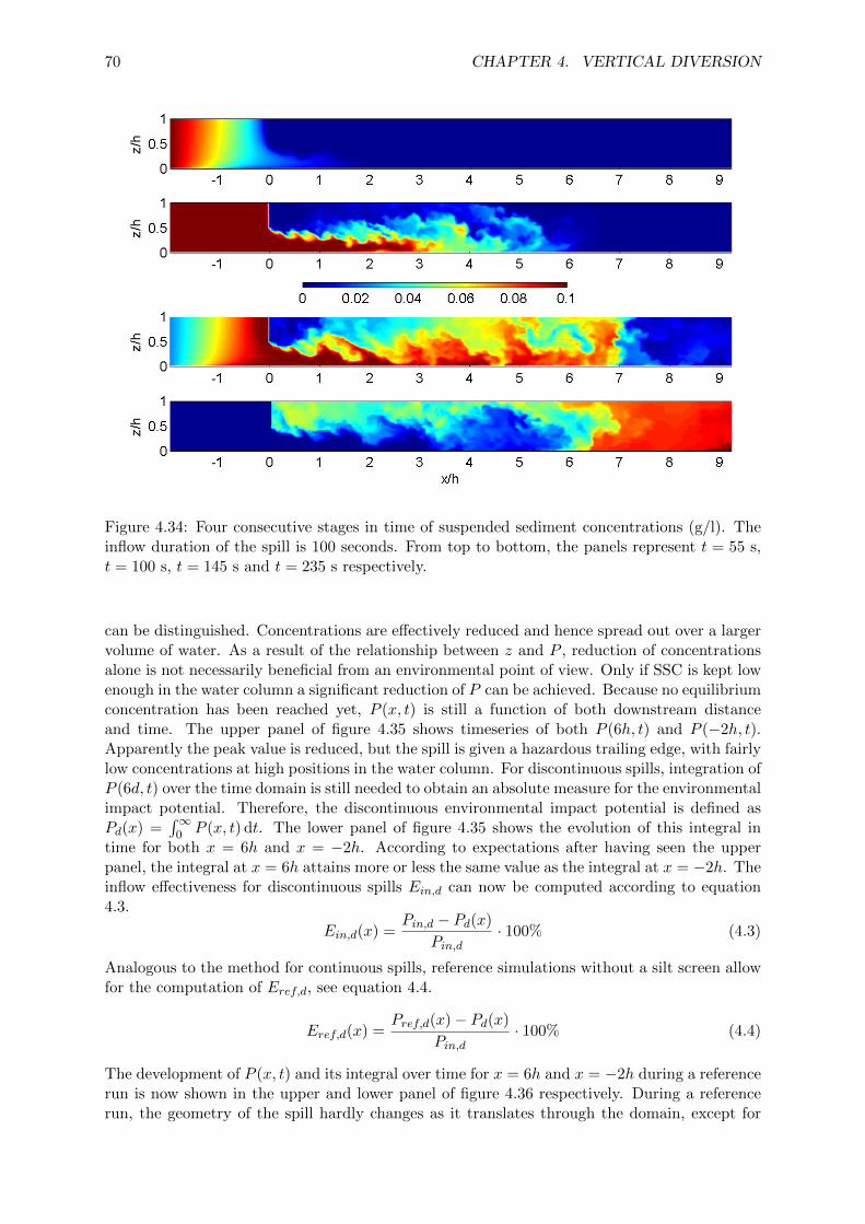
70 CHAPTER 4. VERTICAL DIVERSION
Figure 4.34: Four consecutive stages in time of suspended sediment concentrations (g/l). Theinflow duration of the spill is 100 seconds. From top to bottom, the panels represent t = 55 s,t = 100 s, t = 145 s and t = 235 s respectively.
can be distinguished. Concentrations are effectively reduced and hence spread out over a largervolume of water. As a result of the relationship between z and P , reduction of concentrationsalone is not necessarily beneficial from an environmental point of view. Only if SSC is kept lowenough in the water column a significant reduction of P can be achieved. Because no equilibriumconcentration has been reached yet, P (x, t) is still a function of both downstream distanceand time. The upper panel of figure 4.35 shows timeseries of both P (6h, t) and P (−2h, t).Apparently the peak value is reduced, but the spill is given a hazardous trailing edge, with fairlylow concentrations at high positions in the water column. For discontinuous spills, integration ofP (6d, t) over the time domain is still needed to obtain an absolute measure for the environmentalimpact potential. Therefore, the discontinuous environmental impact potential is defined asPd(x) =
∫∞0 P (x, t) dt. The lower panel of figure 4.35 shows the evolution of this integral in
time for both x = 6h and x = −2h. According to expectations after having seen the upperpanel, the integral at x = 6h attains more or less the same value as the integral at x = −2h. Theinflow effectiveness for discontinuous spills Ein,d can now be computed according to equation4.3.
Ein,d(x) =Pin,d − Pd(x)
Pin,d· 100% (4.3)
Analogous to the method for continuous spills, reference simulations without a silt screen allowfor the computation of Eref,d, see equation 4.4.
Eref,d(x) =Pref,d(x)− Pd(x)
Pin,d· 100% (4.4)
The development of P (x, t) and its integral over time for x = 6h and x = −2h during a referencerun is now shown in the upper and lower panel of figure 4.36 respectively. During a referencerun, the geometry of the spill hardly changes as it translates through the domain, except for

4.2. NUMERICAL MODEL 71
Figure 4.35: Development of environmental impact parameters in time for the same discontinu-ous run. The upper panel shows P (x, t) for x = 6h as well as x = −2h. The lower panel showsthe same curves integrated over the time domain
∫ t0 P (x, t) dt.

72 CHAPTER 4. VERTICAL DIVERSION
Figure 4.36: Development of environmental impact parameters in time during the referencesimulation. P (6h, t) and P (−2h, t) are shown in the upper panel and their time-integratedcounterparts are shown in the lower panel.

4.2. NUMERICAL MODEL 73
Figure 4.37: Discontinuous inflow effectiveness Ein,d(6h) as a function of θ and hrel for concen-tration profile U1.
some settling and some longitudinal diffusion. The former leads to a very slight decrease of thetime-integrated impact potential over downstream distance x. From the lower panels of figure4.35 and 4.36, the value of Eref,d(6h) belonging to this example simulation can be determined.
In total, 24 discontinuous dredging spills have been simulated. For inflow duration ts the values100 s and 500 s were adopted. With the incorporation of ts as a relevant parameter, an additionaldimensionless number can be constructed, see equation 4.5.
α =Utsh
(4.5)
In physical terms, α represents the aspect ratio of the dredging spill, being the ratio of itsinitial length over the water depth. It is a measure for the length of spill boundary exposed tolarge concentration gradients. Big values of α imply a (geometrically) long spill, which has lesspotential to mix thoroughly with ambient clear water. For small values of α this is the otherway around. For continuous spills, α goes to infinity. Figure 4.37 shows the discontinuous infloweffectiveness Ein,d(6d) for concentration profile U1 in the dimensionless θ-hrel plane. The figuredoes not reveal dependency of the effectiveness on α. However, every data point representsthe mean value of two simulations with different values of α. It is found that the effectivenessdepends only marginally on α (deviations remain within 3%) and is largely determined byhrel and θ. Only 6 data points are obtained, but yet they show a clear trend. For increasingθ, the effectiveness increases as well. Thus, the more settling can take place, the higher thediscontinuous inflow effectiveness gets. This corresponds to the previously drawn conclusionsregarding continuous spill. A relation with hrel is less evident. At higher θ a slightly negativerelation seems to exist between Ein,d and hrel as a result of extensive mixing at higher relativescreen height. The values in figure 4.37 correspond well to those obtained for continuous spill(figure 4.25).

74 CHAPTER 4. VERTICAL DIVERSION
Figure 4.38: Discontinuous inflow effectiveness Ein,d(6h) as a function of θ and hrel for concen-tration profile U3.
A similar analysis can be carried out for inflow profile U3. The result is shown in figure4.38. Again, the effectiveness is displayed as a function of hrel and θ. Deviations due to varyingα range up to 6%. In contrast to inflow profile U1, now a positive relation exists between Ein,dand hrel. More intense screen-induced mixing transports more sediment to lower z-coordinates.Again, the results for discontinuous spills with inflow profile U3 closely resemble those forcontinuous spills (figure 4.27).
The lower panel of figure 4.36 already revealed that in a reference simulation Pd only changesvery slowly over downstream distance x. Therefore, the discontinuous reference effectivenessEref,d(6h) is expected to be of the same order as Ein,d(6d). Eref,d(6d) is shown in figure 4.39 and4.40 for profile U1 and U3 respectively. Only the data points with hrel = 0.25 show significantdifferences with the continuous reference effectiveness Eref . This is caused by the fact thatthese data stem from simulations with U = 0.1 m/s. The smaller intensity of wall turbulencegives rise to a high Richardson number. Instable horizontal (profile U1) or vertical (profileU3) stratification leads to a collapse of the concentration profile during reference simulations.Negative buoyancy moves high concentrations to a lower position in the water column, whicheffectively decreases P . This behaviour is considered an artifact of the schematic sedimentprofiles with sharp concentration gradients and is therefore ignored. The values of Eref,d athigher hrel are of the same order as their counterparts for continuous spill (figure 4.28 and4.29).
In summary, the effectiveness of silt screens may be regarded insensitive to the inflow durationof the dredging spill. Although concentrations are reduced stronger for a short inflow duration,the percentage of the total sediment mass passing at every downstream z-coordinate is equalfor continuous and discontinuous spills.

4.2. NUMERICAL MODEL 75
Figure 4.39: Discontinuous reference effectiveness Eref,d(6h) as a function of θ and hrel forconcentration profile U1.
Figure 4.40: Discontinuous reference effectiveness Eref,d(6h) as a function of θ and hrel forconcentration profile U3.

76 CHAPTER 4. VERTICAL DIVERSION
Figure 4.41: Parameters used to derive dimensionless forms of um and x.
4.2.5 Self-similarity analysis
In section 2.2, some aspects of self-similarity were addressed for hydraulic jumps and wall jets.Here, self-similarity analysis is applied to the numerical model results regarding vertical diver-sion. The findings can be related to those of section 2.2.
First of all, the evolution of um(x) is addressed, being the maximum time-averaged stream-wise velocity in every vertical profile. um(x) reaches a maximum near the point of biggestflow contraction. Further downstream it decreases towards the maximum value occurring in alogarithmic flow profile. A dimensionless form of um(x) is obtained following equation 4.6. Infigure 4.41 all parameters used in this self-similarity analysis are indicated.
um(x) =um(x)− Uum0 − U
(4.6)
U denotes the undisturbed depth-averaged streamwise flow velocity and um0 is the maximumvalue of um(x). U is used here as a measure for the maximum velocity occurring in an undis-turbed logarithmic flow profile.
Furthermore, x is made dimensionless by means of length scale L50, being the horizontaldistance between the positions x1 where um(x) = um0 and x2 where um(x) = U+0.5(um(x)−U),corresponding to 50% velocity decay. This is expressed by equation 4.7.
x =x− x1L50
(4.7)

4.2. NUMERICAL MODEL 77
Figure 4.42: Dimensionless velocity decay profiles for silt screens (markers, colourscale indicatesrelative screen height hrel), free jumps (solid line) and wall jets (dotted line).
The use of L50 as a horizontal scaling parameter for velocity decay has been proposed by Longet al. (1990) in their study of submerged hydraulic jumps. They found that this parameterleads, rather than any parameter related to the initial jet height, to the best collapse of velocitydecay profiles onto a single line. Their approach was adopted by various authors later on (e.g.Wu and Rajaratnam, 1995; Dey and Sarkar, 2006; Dey et al., 2010). This also follows fromanalysis of the silt screen data, as scaling with parameters related to the screen height does notyield consistent results.
For every simulation of the basic dataset, 11 data points have been extracted from thesimulation results downstream of the point of maximum flow contraction. Furthermore, thepresented relations of um(x) for free jumps and wall jets (see figure 2.6) have been reworked tomatch the definitions of um and x. Figure 4.42 shows the result. Although the data show a highdegree of scatter, the figure reveals dependency of the velocity decay on hrel. It can roughly besaid that for high hrel the profile is free jump-like, whereas for low hrel it is more wall jet-like.
Now the vertical profiles of time-averaged streamwise velocity are assessed. This calls for newdefinitions. A dimensionless form of u is obtained by means of the maximum velocity um ineach vertical profile, see equation 4.8.
u(z) =u(z)
um(4.8)
The z-coordinate is made dimensionless by means of z1, being the vertical position whereu = 0.5um and ∂u/∂z < 0. This results in z, see equation 4.9.
z =z
z1(4.9)

78 CHAPTER 4. VERTICAL DIVERSION
Figure 4.43: Vertical profiles of dimensionless streamwise time-averaged velocity u. Thecolourscale indicates relative screen height hrel.
Reference height z1 is only defined within the recirculation zone and in the first phase of flowrecovery. Again, the use of z1 as a relevant scaling parameter for vertical profiles of u wasproposed first by Long et al. (1990) and adopted by Wu and Rajaratnam (1995), Dey andSarkar (2006) and Dey et al. (2010). For their wall-jet and submerged jump data as well as thesilt screen data, parameters related to the initial jet height do not lead to satisfactory collapseof the u-profiles. For every simulation of the basic dataset a number of velocity profiles hasbeen extracted downstream of the point of maximum flow contraction. All profiles are plottedin dimensionless form in figure 4.43. Again a lot of scatter is present in the data. The profilesreveal dependency of u(z) on hrel. Even for the same value of hrel the profiles do not collapseonto a single line. This might be caused by dependency on the Froude number.

79
Chapter 5
Horizontal diversion
Depending on the specific application of a silt screen, a cross current might be able to flowaround the side edges. The presence of a silt screen will induce some surface elevation at theupstream side. If the side edges do not connect to a slope or quay wall, the free surface willexhibit a lateral slope. This induces horizontal diversion of the cross current. Depending on thescreen’s geometry, a certain distribution will be established between horizontally and verticallydiverted flow. Determining this distribution as a function of flow velocity, water depth, siltscreen width and silt screen height is the aim of this chapter.
As indicated in chapter 3, horizontal diversion will be modelled by means of a 2DH CFDmodel constructed with the FINEL2D code. The set-up and characteristics of this model arediscussed in section 5.1. Section 5.2 deals with the different scenarios which are investigatedwith the model. Finally, the results of the simulations are presented in section 5.3.
5.1 Set-up
FINEL2D solves the shallow water equations by means of the finite element method. This allowsfor the use of unstructured, triangular grids. The model’s external boundaries form a largerectangle at some distance from the silt screen. The screen itself is represented as an internalboundary. On each edge belonging to the internal boundary, the discharge relation presentedin equation 5.1 is imposed. It is derived from applying conservation of energy upstream andconservation of momentum downstream.
Qs = Beµc(1− hrel)h√
2g(H1 − h2) (5.1)
In this equation, Qs is the discharge across the edge, Be is the length of the edge, µc denotes thecontraction coefficient, H1 = h1 +U2
1 /2g is the upstream energy head and h2 is the downstreamwater depth. It should be noted that this relation only holds for the subcritical flow regime.In chapter 2 it was already shown that the assumption of subcritical flow is justified. Thecontraction coefficient is not a constant, but varies with the boundary conditions. However,from the experiments and simulations regarding vertical diversion it has been determined thatµc = 0.6 is a close approximation for all conditions.
When the external boundaries are situated too close to the silt screen, the distribution ofdischarges is influenced by the boundary conditions. Therefore the model’s geometry is madedependent on the width of the silt screen Ws. Sensitivity analysis has led to the geometrypresented in figure 5.1. The grid resolution can be seen to vary in space, with the finest gridcell size next to the silt screen and coarsening towards the external boundaries.
It is mentioned in appendix F.3 that FINEL2D does not include turbulent shear stresses andis therefore limited to flows dominated by advection. The downstream ‘wake’ of a silt screen

80 CHAPTER 5. HORIZONTAL DIVERSION
Figure 5.1: Geometry of the 2DH model. The red line indicates the position of the silt screen,which is modelled as an internal discharge boundary.
is certainly influenced by turbulent diffusion, making the results concerning this region ratherdoubtful. However, this study focuses on the upstream process of horizontal diversion, whichis dominated by advection. The water level right downstream of the silt screen still appearsin the discharge relation (equation 5.1). However, sensitivity analysis has shown that Qs ishardly influenced by the downstream flow conditions. For example, under certain conditionsthe wake does no longer exhibit stationary behaviour and attains the character of a vortexstreet. FINEL2D can not be trusted unconditionally on correct prediction of this behaviour,but the predicted discharge across the silt screen is still consistent with other simulations.
5.2 Scenarios
Before the actual 2DH simulation scenarios are discussed, the relevant parameters will be de-rived from dimensional analysis. Inclusion of the second horizontal dimension introduces thesilt screen’s width Ws as an additional parameter. Just like the screen’s height, it is madedimensionless through dividing by the water depth. The resulting parameter W∗ = Ws/h is ameasure for horizontal diversion. The bigger W∗, the more difficult it will be for the currentto flow around the side edges of the screen. The Froude number, based on undisturbed U andh, serves as a measure for the load acting on the silt screen. A higher load will induce morehorizontal diversion.
Horizontal diversion itself can be quantified as the rate of the vertically diverted dischargeover the total inflowing discharge along the width of the screen. With n the number of gridedges constituting the silt screen, the relative discharge Qrel is given by equation 5.2.
Qrel =
∑n1 Qs
UhWs· 100% (5.2)
The relative discharge denotes the percentage of the flow which is being diverted vertically. Itshould be clear that vertical diversion is the intended effect of a silt screen, whereas horizontaldiversion should be limited as much as possible. This corresponds to a high relative discharge.
Now the actual 2DH simulation scenarios are presented. Table 5.1 lists the different values of
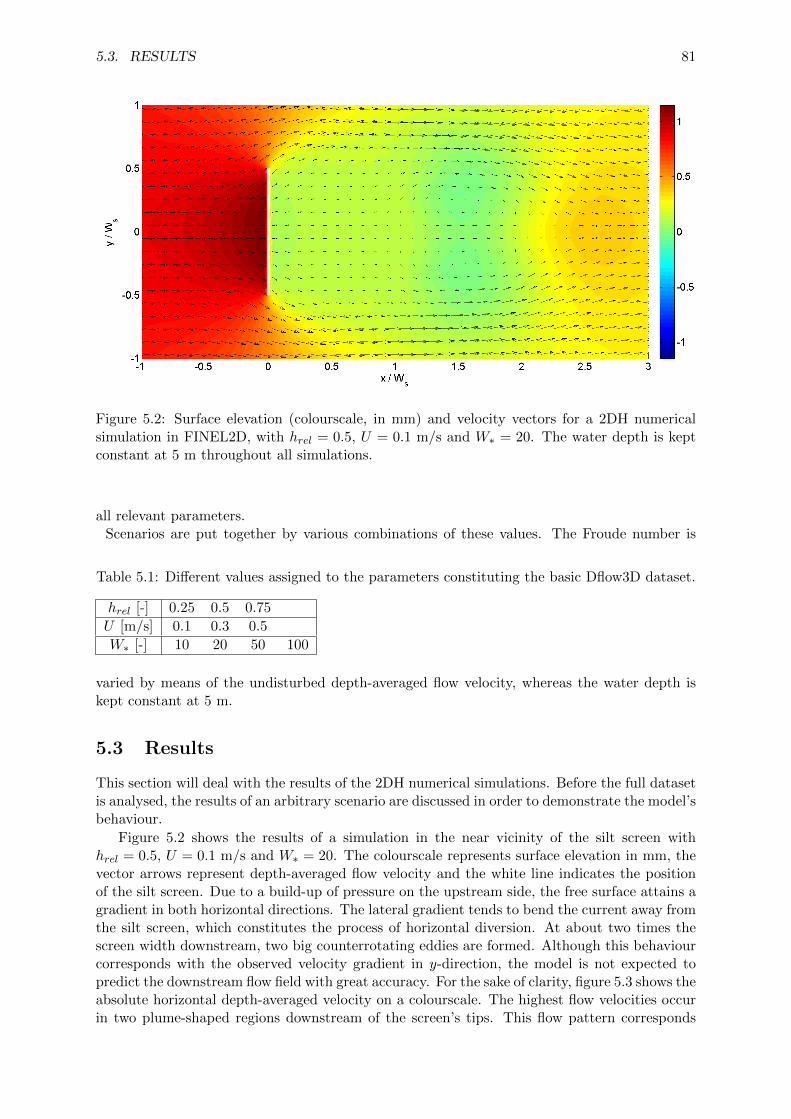
5.3. RESULTS 81
Figure 5.2: Surface elevation (colourscale, in mm) and velocity vectors for a 2DH numericalsimulation in FINEL2D, with hrel = 0.5, U = 0.1 m/s and W∗ = 20. The water depth is keptconstant at 5 m throughout all simulations.
all relevant parameters.Scenarios are put together by various combinations of these values. The Froude number is
Table 5.1: Different values assigned to the parameters constituting the basic Dflow3D dataset.
hrel [-] 0.25 0.5 0.75
U [m/s] 0.1 0.3 0.5
W∗ [-] 10 20 50 100
varied by means of the undisturbed depth-averaged flow velocity, whereas the water depth iskept constant at 5 m.
5.3 Results
This section will deal with the results of the 2DH numerical simulations. Before the full datasetis analysed, the results of an arbitrary scenario are discussed in order to demonstrate the model’sbehaviour.
Figure 5.2 shows the results of a simulation in the near vicinity of the silt screen withhrel = 0.5, U = 0.1 m/s and W∗ = 20. The colourscale represents surface elevation in mm, thevector arrows represent depth-averaged flow velocity and the white line indicates the positionof the silt screen. Due to a build-up of pressure on the upstream side, the free surface attains agradient in both horizontal directions. The lateral gradient tends to bend the current away fromthe silt screen, which constitutes the process of horizontal diversion. At about two times thescreen width downstream, two big counterrotating eddies are formed. Although this behaviourcorresponds with the observed velocity gradient in y-direction, the model is not expected topredict the downstream flow field with great accuracy. For the sake of clarity, figure 5.3 shows theabsolute horizontal depth-averaged velocity on a colourscale. The highest flow velocities occurin two plume-shaped regions downstream of the screen’s tips. This flow pattern corresponds

82 CHAPTER 5. HORIZONTAL DIVERSION
Figure 5.3: Absolute horizontal depth-averaged velocity (colourscale, in m/s) and the associatedvelocity vectors for the same simulation.
well with the flow pattern around blunt objects, e.g. a groyne (Schiereck, 2001).The discharge through the grid edges representing the silt screen is shown in dimensionless
form in figure 5.4. The solid line represents the relative specific discharge qrel = Qs/(BeUh) asa function of the screen’s y-coordinate. Zero horizontal diversion corresponds with the dottedline. The ratio of the surface underneath the solid line over the surface underneath the dottedline is equal to Qrel. The influence of horizontal diversion intensifies towards the side edges.
By evaluating the ratio of these integrals, Qrel is determined for all simulations. These per-centages are shown in figure 5.5 as a function of Fr/W∗ and hrel. The black markers show theactual datapoints. Contours of equal Qrel are determined from interpolation. The dimension-less parameter Fr/W∗ is a measure for the ease of horizontal diversion, whereas hrel representsthe resistance against vertical diversion. Some trivial features can be recognized in the figurestraight away:
• For an infinitely long silt screen, Fr/W∗ approaches zero. In that case, Qrel approaches100%, as flow around the screen’s side edges will not be possible.
• For hrel = 0, the flow is not hampered by the screen and Qrel should equal 100%. Anegative relation between Qrel and hrel is visible in the figure, but linear extrapolation ofthe contours towards hrel = 0 leads to a smaller relative discharge than 100%. Therefore,a stronger relation between both parameters will exist for small relative screen heights.
• For hrel = 1, the screen blocks the flow completely and Qrel should equal 0%. This alsofollows from linear extrapolation of the contours.
Horizontal diversion is an unwanted effect of silt screen application at open water. Only if thevast majority of a dredging spill passes underneath the silt screen, possibly favourable effectsof vertical diversion might take place. The figure shows that this is only bound to happen atextremely low Froude numbers and/or extremely long silt screens. In any case, the relativescreen height should be kept small in order to promote vertical diversion. A certain degree ofhorizontal diversion can never be avoided. This leads to increased dispersion and diffusion ofthe dredging spill, which decreases effectiveness.

5.3. RESULTS 83
Figure 5.4: Relative specific discharge qrel through the grid edges representing the silt screen(solid line). The horizontal axis shows the lengthwise coordinate of the screen. In case of nohorizontal diversion, the solid line equals the dotted line.
Figure 5.5: Relative discharge Qrel as a function of Fr/W∗ and hrel. The actually obtaineddata are indicated by black triangles. Contour lines are constructed by means of interpolation.

84 CHAPTER 5. HORIZONTAL DIVERSION

85
Chapter 6
Adjustments
The secondary goal of this research is to test a number of promising adjustments to the hangingsilt screen. These adjustments are divided into two categories. Adjustments to the large-scaleapplication involve the use of ‘ordinary’ hanging silt screens in new formations. They arediscussed in section 6.1. Adjustments to the small-scale design involve actual adaptations tothe silt screen itself. These are dealt with in section 6.2.
It is stressed that this chapter does not aim to deliver a ready-to-use improved design forhanging silt screens. If conclusions regarding a promising adjustment are positive, furtherresearch should be conducted in order to determine its feasibility, its constructability and itsbehaviour under various circumstances.
6.1 Large-scale application
In appendix B a number of different large-scale applications of hanging silt screens are listed.These include oblique placement of the screen with respect to the current, V-shaped placement,leaving a gap between adjacent sections of the screen, application as a diffuser and placing twoscreens after another. However, some remarks have to be made regarding these applications:
• Although oblique placement and V-shaped placement might seem comparable applica-tions, there is an important difference. Both options aim at diverting the plume hori-zontally in a streamlined way. Discharge ‘through’ the screen will only cease if pressuredifferences between both sides are kept small. In case of V-shaped placement, a down-stream wake with low pressures is unavoidable, which induces a significant amount ofvertical diversion. This drawback does not necessarily hold for oblique screen placement,since the current might bend completely into the wake at the downstream side of thescreen. Theoretically there would be no pressure difference between both sides. Becauseof these considerations, only oblique placement is actually investigated.
• The adjustments aiming at extensive mixing of the plume should be investigated in a2DH set-up. In this research, 2DH modelling is done by means of FINEL2D. Exclusionof turbulent shear stresses from the governing equations and high numerical diffusionlimit the use of this code to flows dominated by advection. Therefore it is not possibleto include these adjustments in this research. From chapter 4 and 5 it is known thatextensive diffusion often leads to a negative effectiveness. Furthermore it is not very likelythat diffusing a turbidity plume by means of silt screens reduces concentrations far enoughto fit within environmental legislation. Hence these adjustments are not considered verypromising.
Now, oblique placement and application of two silt screens will be discussed consecutively inthe remainder of this section.

86 CHAPTER 6. ADJUSTMENTS
Figure 6.1: Absolute depth-averaged horizontal flow velocity (colourscale, m/s) and the asso-ciated velocity vectors in the near vicinity of an obliquely placed silt screen with d = 5 m,hrel = 0.5, U = 0.3 m/s, W∗ = 20 and β = 45◦.
6.1.1 Oblique placement
The result of a FINEL2D simulation with an obliquely placed screen is shown in figure 6.1.This concerns a simulation with U = 0.3m/s, hrel = 0.5, W∗ = 20 and silt screen rotation angleβ = 45◦. The colourscale and vector arrows both indicate absolute depth-averaged horizontalflow velocity. The obliquely placed screen does not function as intended:
• The regions of high flow velocity downstream of both tips indicate that horizontal diversionis still taking place to both sides. Ideally, all diverted fluid should end up to the left side ofthe screen (as seen from the upstream side). This process can be quantified by determininghow many percent of the inflowing discharge at the upstream model boundary ends uppassing the silt screen left (46.3%), right (47.7%) or underneath (6.0%). It appears thatthe obliquely placed screen diverts flow to the unintended side rather than to the intendedside.
• Furthermore, the screen still has a long wake with low flow velocities. The big pressuredifference leads to a significant discharge through the screen. When compared to a per-pendicular screen, the influence of β on Qrel can be expressed as the ratio of the totaldischarge through the screen at angle β over the total discharge through a perpendicularscreen of the same width when projected on the y-axis: Qrel(β)/(Qrel(0) cosβ) · 100%.For the current simulation, that results in 117%. Apparently, the obliquely placed screenattracts a bigger percentage of the total discharge than a perpendicularly placed screen.
These observations hold for all simulations. Figure 6.2 shows the ratio of the total dischargepassing the screen on the left side over the right side, QL/QR, as a function of β. The solid linesconnect simulations with equal hrel, U and W∗. A clear relationship between these parametersand the discharge ratio can not be found. Nevertheless, except for one simulation, obliquenessof the silt screen diverts the biggest part of the current to the right.
In figure 6.3, Qrel is shown as a function of β. Again, the solid lines connect simulations withequal conditions. For all conditions, Qrel grows as β grows, indicating that oblique placement

6.1. LARGE-SCALE APPLICATION 87
Figure 6.2: Ratio between total discharge passing the screen at the left side over the right side,as seen from the upstream side. Except for one simulation, a rotated screen diverts the biggestpart of the discharge towards the right side.
Figure 6.3: Relative discharge Qrel as a function of rotation angle β. Qrel represents the ratioof the total discharge passing the oblique screen over the discharge through a perpendicularscreen of the same width when projected on the y-axis.

88 CHAPTER 6. ADJUSTMENTS
attracts a bigger part of the current to the silt screen.
Altogether, oblique placement leads to less horizontal diversion, which is contrary to the in-tended effect. Furthermore, the biggest part of the current is diverted around the upstream tipof the screen, which is contrary to the intended effect as well. So only if the turbidity plume islocated in the upper half of figure 6.1, the silt screen redirects the plume towards the intendeddirection. Though it should be noted that this effect is even stronger with the screen placedperpendicular to the current.
6.1.2 Two silt screens
In appendix B, placing two consecutive silt screens is presented as a possible way of ‘halting’a turbidity plume. In between both screens a fixed recirculation zone will form, which mightabsorb a significant part of an initial turbidity plume. However, an exchange current will beformed between the recirculation zone and the main flow. Eventually all turbidity will endup downstream of both screens, which indicates that the halting effect is only of temporarynature. Nevertheless this adjustment is expected to result in extensive horizontal dispersion.Concentrations might be brought low enough in the water column to reduce the environmentalimpact potential.
First, the performance of Dflow3D in case of two consecutive silt screens is validated by compar-ing numerical simulation results to the results of laboratory experiment 2G. Figure 6.4 shows u,w, ru, rw and τ ′uw respectively from top to bottom. The numerical model performs fairly well,although it underestimates the maximum time-averaged streamwise velocity downstream of thesecond silt screen. The resulting smaller velocity shear consequently affects the turbulence pa-rameters. The smaller maximum jet velocity seems to result from a slightly different relativescreen height. Due to the discrete nature of the numerical grid, hrel can not be implemented atits exact value. Hence it is very likely that the observed differences between the physical andnumerical models do not stem from fundamental errors produced by the numerical code. Thereis no reason to believe that Dflow3D performs worse with two silt screens than with a singleone.
Now the simulation results regarding silt screen effectiveness are presented. Again a distinctionis made between continuous and discontinuous spills. The former is addressed first. Simula-tions were conducted with hrel = 0.75, U = 0.3 m/s, ws = 1 mm/s, d = 5 m and concentrationprofiles U2 and U3. Time-averaged SSC for profile U2 is depicted in figure 6.5. The lower panelshows the reference simulation. Due to its low position in the water column, the biggest partof the plume passes both screens with the main flow. Only very low concentrations are storedin the first recirculation zone. Downstream of the second silt screen, extensive dispersion anddiffusion spreads SSC equally over the full water depth. This behaviour is similar to the sit-uation with one screen. The integrated environmental impact potential and both effectivenessparameters are shown in figure 6.6. At a distance of 30 m downstream of the second screen,Ein(9h) = −66% and Eref (9h) = −65% are found. Figure 4.26 predicts a less negative value ofEin(6d) in case of a single screen with hrel = 0.75 and θ = 3.3 · 10−3. Apparently two screenscause even more sediment to end up in the upper part of the water column.
Figure 6.7 shows suspended sediment concentrations for profile U3. The first recirculationzone is filled with high concentrations. As the plume is continuous, an equilibrium situation hasbeen reached. Hence, the recirculation zone absorbs as much sediment as it releases into themain flow. Continuity now requires that the flux of SSC passing the second screen is the equalto the flux passing the first screen. Compared to a situation with only one screen, increasedmixing might be the only difference. P (x), Ein(x) and Eref (x) are presented in figure 6.8. The

6.1. LARGE-SCALE APPLICATION 89
Figure 6.4: Validation plot for laboratory run 2G. From upper to lower panel, the time-averagedvelocities u and w, turbulence intensities ru and rw and Reynolds stress τ ′uw are shown.

90 CHAPTER 6. ADJUSTMENTS
Figure 6.5: Time-averaged suspended sediment concentrations C for a numerical simulationwith two silt screens. Inflowing concentration profile U2 is applied.
Figure 6.6: Environmental impact potential P (x) (upper panel), inflow effectiveness Ein(x)(middle panel) and reference effectiveness Eref (x) (lower panel) for a numerical simulation withtwo silt screens and concentration profile U2.

6.1. LARGE-SCALE APPLICATION 91
Figure 6.7: Time-averaged suspended sediment concentration C for a numerical simulation withtwo silt screens. The concentration profile is U3.
Figure 6.8: P (x), Ein(x) and Eref (x) for a numerical simulation with two screens and concen-tration profile U3.

92 CHAPTER 6. ADJUSTMENTS
Figure 6.9: Discontinuous impact parameters for a simulation with two silt screens, concen-tration profile U3 and an inflow duration of 100 s. The upper panel shows the environmentalimpact potential as a function of time both at inflow and at 6h downstream of the second screen.The lower panel shows the development of both integrals in time.
values at 30 m downstream of the second screen are only a little bit higher than the valuespredicted by figure 4.27 and 4.29: Ein(9h) = 29% and Eref (9h) = 10%. Probably the highervalue results from increased vertical mixing, which directs more sediment towards the lower halfof the water column.
Fundamentally different behaviour is expected for discontinuous plumes. The increased hori-zontal dispersion will lead to lower concentrations over a longer period of time. In chapter 4 itwas argued that such a diffusive trailing edge is only beneficial if concentrations are brought toa lower position in the water column.
Figure 6.9 shows P (x, t) and its integral in time for both the inflow profile and the profileat six times the water depth downstream of the second screen. The inflow profile is U3 andinflow duration ts = 100 s. The discontinuous effectiveness parameters are Ein,d(9d) = 31%and Eref,d(9d) = 12%. In this simulation, α = 6, θ = 3.3 · 10−3 and hrel = 0.75 when screendeformations are not taken into account. The presented values of Ein,d and Eref,d are slightlymore positive as those for a comparable simulation with only one screen, see figure 4.38 and4.40. This can be explained by the more intense downstream mixing imposed by two silt screensinstead of one. Inflow profile U3 is diffused over the full water column more effectively, whichleads to a lower environmental impact potential. This is solely the effect of intense mixing. Dueto the extended stretch over which increased bed shear stress occurs, the amount of depositionis expected to decrease and the amount erosion is expected to increase. Hence conclusionsregarding the application of two consecutive silt screens may only be moderately positive whenfacing a discontinuous spill with most upstream SSC located at high z-coordinates.

6.2. SMALL-SCALE DESIGN 93
6.2 Small-scale design
Some of the adjustments which are suggested in appendix B involve modifications to the designof silt screens. These adjustments are a perforated screen and extension of the lower edge witha flap. For technical reasons, both adjustments can not be implemented in Dflow3D. Thereforethe analysis is limited to the laboratory experiments.
6.2.1 Perforated screen
Conventional hanging silt screens completely block a part of the water column. This leads tohigh jet velocities underneath the screen and big velocity gradients downstream. Continuityrequires dispersion of the jet flow over the full water depth. Increased turbulent diffusion due tothe big velocity gradient leads to extensive mixing of suspended sediment concentrations. In thatway the impermeability of silt screens undermines their objective to reduce the environmentalimpact potential.
A possible design adjustment to overcome these drawback is to make a silt screen partiallypermeable. The resulting decrease of velocity shear accordingly leads to less dispersion anddiffusion. However, a permeable silt screen will also allow for a part of the turbidity plume topass through the screen. This gives rise to SSC in the upper part of the water column. Whetherthe beneficial or the detrimental effect of a perforated screen dominates the resulting situationis not known beforehand.
A number of important notions must be kept in mind when designing perforated silt screens.
• The detrimental effect of perforation can be limited by applying a permeability gradientover depth. Ideally, the screen’s permeability should decrease from 100% near the loweredge to 0% near the free surface.
• The size of the perforations governs the size of the turbulent structures issuing from them.Transport of suspended solids is mainly associated with the biggest structures in the flow.As increased mixing should be prevented, small holes are preferred.
The first notion can not be realised without changing the design of conventional silt screensdrastically. This research into possible improvements should start with assessing what can bedone with relatively simple adjustments.
Two laboratory experiments are conducted with perforated silt screens. The design asapplied in experiment 2D is depicted in figure 6.10. This design leads to an average permeabilityof 8%. Figure 6.11 shows the results of experiment 2D and experiment 2B, which serves as areference experiment with an impermeable screen. The upper panel, showing time-averagedhorizontal flow velocity u, indicates that both the maximum jet flow velocity and the maximumreturn velocity are decreased. This matches expectations, since the discharge of the jet flowis lower than the total discharge. Less velocity shear also leads to significantly less turbulenceproduction, which is reflected by ru, rw and τ ′uw in the lower three panels. The same trends,though less explicit, are observed for experiment 2C, which has a permeability of only 3%.
Unfortunately these laboratory experiments only give an indication of the beneficial effectof perforated silt screens, as the output is limited to flow-related parameters. Although thedecrease of Reynolds stresses is quite spectacular given the low average permeability of thescreen, information on the detrimental effect is needed to give a final judgment on this designadjustment.
Without further research, it is not known where optimisation of silt screen permeabilityleads to. It might be the case that effectiveness keeps increasing for increasing permeability. Ifthis is the case, silt screen effectiveness is optimal for 100% permeability, corresponding to noscreen at all.
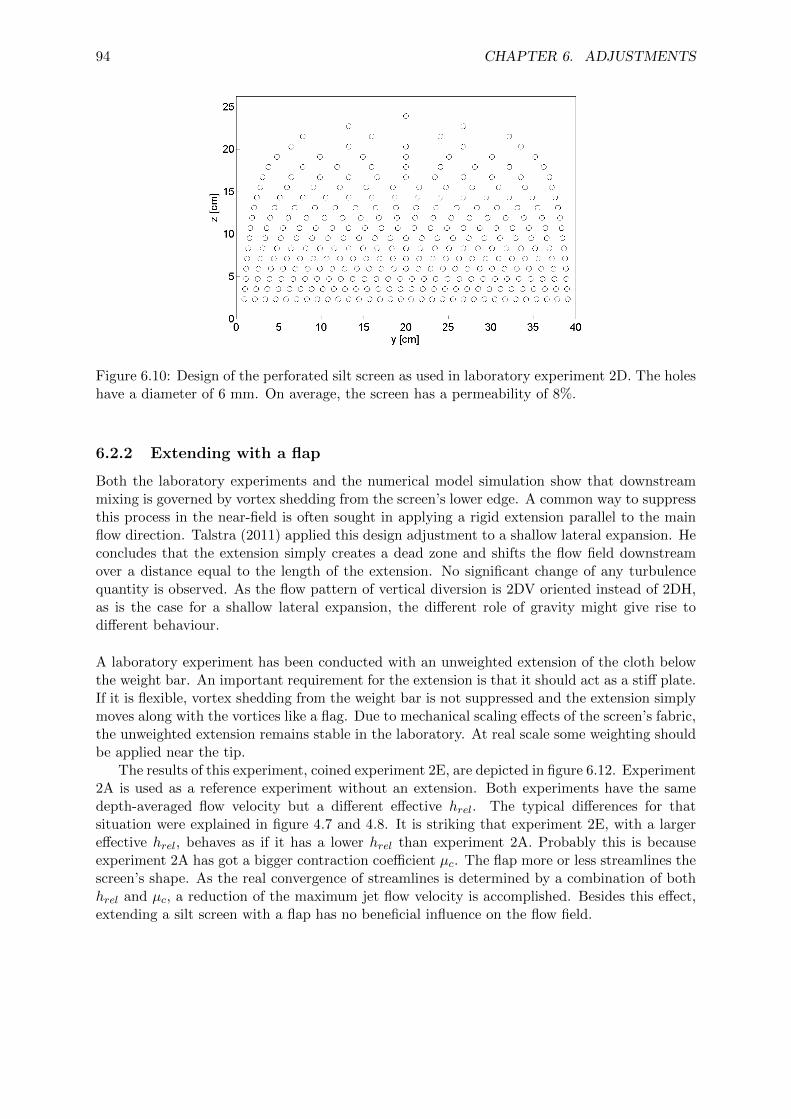
94 CHAPTER 6. ADJUSTMENTS
Figure 6.10: Design of the perforated silt screen as used in laboratory experiment 2D. The holeshave a diameter of 6 mm. On average, the screen has a permeability of 8%.
6.2.2 Extending with a flap
Both the laboratory experiments and the numerical model simulation show that downstreammixing is governed by vortex shedding from the screen’s lower edge. A common way to suppressthis process in the near-field is often sought in applying a rigid extension parallel to the mainflow direction. Talstra (2011) applied this design adjustment to a shallow lateral expansion. Heconcludes that the extension simply creates a dead zone and shifts the flow field downstreamover a distance equal to the length of the extension. No significant change of any turbulencequantity is observed. As the flow pattern of vertical diversion is 2DV oriented instead of 2DH,as is the case for a shallow lateral expansion, the different role of gravity might give rise todifferent behaviour.
A laboratory experiment has been conducted with an unweighted extension of the cloth belowthe weight bar. An important requirement for the extension is that it should act as a stiff plate.If it is flexible, vortex shedding from the weight bar is not suppressed and the extension simplymoves along with the vortices like a flag. Due to mechanical scaling effects of the screen’s fabric,the unweighted extension remains stable in the laboratory. At real scale some weighting shouldbe applied near the tip.
The results of this experiment, coined experiment 2E, are depicted in figure 6.12. Experiment2A is used as a reference experiment without an extension. Both experiments have the samedepth-averaged flow velocity but a different effective hrel. The typical differences for thatsituation were explained in figure 4.7 and 4.8. It is striking that experiment 2E, with a largereffective hrel, behaves as if it has a lower hrel than experiment 2A. Probably this is becauseexperiment 2A has got a bigger contraction coefficient µc. The flap more or less streamlines thescreen’s shape. As the real convergence of streamlines is determined by a combination of bothhrel and µc, a reduction of the maximum jet flow velocity is accomplished. Besides this effect,extending a silt screen with a flap has no beneficial influence on the flow field.

6.2. SMALL-SCALE DESIGN 95
Figure 6.11: Comparison of a laboratory experiment with a perforated screen (experiment 2D)and its reference experiment (2B). From top to bottom the panels show u, w, ru, rw and τ ′uw.

96 CHAPTER 6. ADJUSTMENTS
Figure 6.12: Results of laboratory experiment 2E. The silt screen has been extended with arigid flap. Experiment 2A is shown as a reference. From top to bottom the panels show u, w,ru, rw and τ ′uw.

97
Chapter 7
Conclusions
In this thesis the effectiveness of hanging silt screens in cross flow has been investigated. Itis known that in present-day dredging practice hanging silt screens are considered an effectiveenvironmental measure under mild flow conditions. After fundamental research, involving liter-ature study, physical modelling and numerical modelling, it becomes clear that earlier reportson hanging silt screen effectiveness have been too positive.
The findings of this research are formulated in 9 conclusions:
1. Vertical diversion of sediment-laden flow caused by hanging silt screens has a negativeeffect on the spreading of suspended sediment, regardless of local conditions and siltscreen geometry.
2. The effectiveness of silt screens is insensitive to the duration of a dredging spill. Thescreen gives rise to large diffusion in streamwise direction, but the influence of the screenremains equally negative.
3. If a dredging spill is mainly situated in the lower half of the water column, silt screenshave the most negative impact.
4. Comparing downstream SSC to upstream SSC results in a too positive view on silt screeneffectiveness. All relevant parameters should be compared to the same situation withouta silt screen. Values within five times the water depth downstream of the silt screen arenot representative, as the negative effects need some distance to develop.
5. The definition of the ‘badness’ of suspended sediment, coined ‘environmental impact po-tential’ in this research, should include the influence of SSC values and their height abovethe bed.
6. If erodible bed mass is available, a silt screen will lead to increased erosion.
7. Application of hanging silt screens on open waters causes a significant amount of horizontalflow diversion. This counteracts the intended usage of silt screens as a vertical currentdeflector and brings along increased dispersion and diffusion of SSC.
8. Oblique placement of a silt screen with respect to the current can not be used for intendedhorizontal diversion of a complete dredging spill. It is counterproductive in two ways: (1)the biggest part of the current is diverted to the unintended side and (2) vertical diversionincreases per unit of projected screen width.
9. None of the application or design adjustments investigated in this research irrefutablydemonstrates a positive effect of silt screens on the spreading of suspended sediment.

98 CHAPTER 7. CONCLUSIONS
Bearing these conclusions in mind, it is interesting to revisit the case studies which were previ-ously treated in appendix A. The knowledge gained through this research is applied to the samecases in appendix I, which leads to interesting findings. Especially the occurrence of horizontaldiversion seems to be ignored in a number of cases.

99
Chapter 8
Recommendations
The effectiveness of hanging silt screens in cross flow is not an isolated topic in dredging prac-tice. The application of silt screens is surrounded by a complex decision making process, whichwas briefly explained in chapter 1. Most recommendations are aimed at integrating the con-clusions of this research into the (environmental) management practice of dredging works. Allrecommendations are listed below:
1. Make an effort to convince all parties involved in dredging practice of the ineffectivenessof hanging silt screens in cross flow. In that way requests from clients or local authoritiesfor silt screen application in unfavourable circumstances can be avoided or rejected suc-cessfully. This leads to a better protection of the environment and helps both clients anddredging companies to save expenses on useless mitigation measures.
2. Investigate whether the environmental impact potential as defined in this research can beof use when quantifying environmental impact of dredging projects. A new definition wasbrought up here, as an appropriate way of quantifying the environmental risks of SSCappeared to be lacking. It is expected that the environmental impact potential can beapplied to many different projects, especially those involving numerical modelling. Theexact definition might be subject to debate amongst researchers in the field of ecology.Further improvements to the environmental impact potential are encouraged here.
3. Contrary to hanging silt screens in cross flow, standing silt screens covering the entirewater depth have been proved successful in retaining dredging-induced SSC under verycalm flow conditions. However, standing silt screens have the disadvantage of much stricteroperational, mechanical and hydrodynamical constraints. It is therefore recommended tooptimise guidelines for the application of standing silt screens covering the entire waterdepth.
4. Do not put effort into developing beneficial adaptations to the design or application ofhanging silt screens in cross flow. The adaptations proposed and investigated in thisresearch were deduced systematically with the help of experts in the fields of silt screenapplication, marine biology, turbulent flows and suspended sediment transport. As theseadaptations show no proof of a potential increase in silt screen effectiveness, successfuladaptations are considered non-existent.
Some additional remarks have to be made regarding certain approaches applied and choicesmade in this research. As these remarks are not expected to influence the conclusions in anypossible way, they are not posed as full recommendations requiring further action or research.Nevertheless they are listed below for the sake of completeness:
• The use of the synthetic eddy method (SEM) to create a fully turbulent upstream velocityboundary in reference simulations was mentioned in section 4.2.2. SEM was not applied to

100 CHAPTER 8. RECOMMENDATIONS
the 2DV simulations with a silt screen, as this led to a better validation of the downstreamflow field. To comply with the reference simulations, it would have been sound to imposethe synthetic eddy method at the upstream velocity boundary in all 2DV simulations.
• As an upstream sediment boundary, schematised SSC profiles were imposed. The uniformprofiles, which contain no vertical concentration gradient at all or a very sharp one, wereused the most frequently. Such profiles will never be encountered in practice. Althoughthe results obtained with more realistic profiles, like the linear ones, could be readilylinked to the basic dataset, it would have been better when both linear profiles had beenapplied in the basic dataset.
• Some trouble was encountered with implementing the deformed shape of a silt screen inthe numerical grid of Dflow3D. Although the model’s performance has been validatedsatisfactory using vertical screens, it might have been worth the effort to correct thistechnical issue.

References
Antonopoulos-Domis, M. (1981). Large-eddy simulation of a passive scalar in isotropic turbu-lence, Journal of Fluid Mechanics 104: 55–79.
Bonnecaze, R. T., Hallworth, M. A., Huppert, H. E. and Lister, J. R. (1995). Axisymmetricparticle-driven gravity currents, Journal of Fluid Mechanics 294: 93–121.
Bonnecaze, R. T., Huppert, H. E. and Lister, J. R. (1993). Particle-driven gravity currents,Journal of Fluid Mechanics 250: 339 – 369.
Boot, M. (2000). Near-field verspreiding van het overvloeiverlies van een sleephopperzuiger,Master’s thesis, Delft University of Technology, Delft, Netherlands.
Bray, R. N. (ed.) (2008). Environmental aspects of dredging, Taylor & Francis, Leiden, Nether-lands.
De Wilde, J. J. (1995). Slibschermproeven, Technical report, WL Delft Hydraulics, Delft,Netherlands.
De Wit, L. (2010). Near field 3D CFD modelling of overflow plumes, in Dobson (2010).
Dey, S., Nath, T. K. and Bose, S. K. (2010). Submerged wall jets subjected to injection andsuction from the wall, Journal of Fluid Mechanics 653: 57–97.
Dey, S. and Sarkar, A. (2006). Response of velocity and turbulence in submerged wall jets toabrupt changes from smooth to rough beds and its application to scour downstream of anapron, Journal of Fluid Mechanics 556: 387–419.
Dobson, J. (ed.) (2010). Proceedings of World Dredging Congress XIX, Chida.
Erftemeijer, P. L. A., Riegl, B., Hoeksema, B. W. and Todd, P. A. (2012). Environmentalimpacts of dredging and other sediment disturbances on corals: A review, Marine PollutionBulletin 64: 1737–1765.
Erftemeijer, P. L. A. and Robin Lewis, R. R. (2006). Environmental impacts of dredging onseagrasses: A review, Marine Pollution Bulletin 52: 1553–1572.
Fischer, H. B., List, E. J., Koh, R. C. Y., Imberger, J. and Brooks, N. H. (1979). Mixing inInland and Coastal Waters, Academic Press, San Diego, USA.
Francingues, N. R. and Palermo, M. R. (2005). Silt curtains as a dredging project managementpractice, Technical report, U.S. Army Engineer Research and Development Center, Vicksburg,USA.
Hallworth, M. A., Hogg, A. J. and Huppert, H. E. (1998). Effects of external flow on composi-tional and particle gravity currents, Journal of Fluid Mechanics 359: 109–142.
Hinze, J. O. (1975). Turbulence, McGraw-Hill, New York, USA.
101

102 REFERENCES
Hofland, B. and Battjes, J. A. (2006). Probability density function of instantaneous drag forcesand shear stresses on a bed, Journal of Hydraulic Engineering 132: 1169–1175.
Holthuijsen, L. H. (2007). Waves in Oceanic and Coastal Waters, Cambridge University Press,Cambridge, UK.
Jarrin, N., Benhamadouche, S., Laurence, D. and Prosser, R. (2006). A synthetic-eddy-methodfor generating inflow conditions for large-eddy simulations, International Journal of Heat andFluid Flow 27: 585–593.
JBF Scientific Corporation (1978). An analysis of the functional capabilities and performanceof silt curtains, Technical report, U.S. Army Corps of Engineers, Vicksburg, USA.
Jin, J. Y., Chae, J. W., Song, W. O., Park, J. S., Kim, S. E., Jeong, W. M., Yum, K. D. andOh, J. K. (2003). Behavior of currents and suspended sediments around a silt screen, Oceanand Polar Research 25: 399–408.
Kang, H. S., Chester, S. and Meneveau, C. (2003). Decaying turbulence in an active-grid-generated flow and comparisons with large-eddy simulation, Journal of Fluid Mechanics480: 129–160.
Kirk, J. T. O. (1977). Attenuation of light in natural waters, Australian Journal of Marine andFreshwater Research 28: 497–508.
Launder, B. E. and Rodi, W. (1983). The turbulent wall jet - measurements and modeling,Annual Review of Fluid Mechanics 15: 429–459.
Long, D., Steffler, P. M. and Rajaratnam, N. (1990). LDA study of flow structure in submergedhydraulic jump, Journal of Hydraulic Research 28: 437–460.
Moser, R. D., Kim, J. and Mansour, N. N. (1999). Direct numerical simulation of turbulentchannel flow up to Reτ = 590, Physics of Fluids 11: 943–945.
Nederlands Normalisatie-instituut (2000). NEN-EN-ISO 7027, Delft, Netherlands.
Nicoud, F. and Ducros, F. (1999). Subgrid-scale stress modelling based on the square of thevelocity gradient tensor, Flow, Turbulence and Combustion 62(3): 183–200.
Noh, Y. and Fernando, H. J. S. (1991). Gravity current propagation along an incline in thepresence of boundary mixing, Journal of Geophysical Research 96(C7): 12,586–12,592.
Obi, S., Inoue, K., Furukawa, T. and Masuda, S. (1996). Experimental study on the statisticsof wall shear stress in turbulent channel flows, Intenational Journal of Heat and Fluid Flow21: 576–581.
Pope, S. B. (2000). Turbulent Flows, Cambridge University Press, Cambridge, UK.
Rivera, M. K. (2000). The inverse energy cascade of two-dimensional turbulence, PhD thesis,University of Pittsburgh.
Schiereck, G. J. (2001). Introduction to bed, bank and shore protection, Delft University Press,Delft, Netherlands.
Simpson, J. E. (1987). Gravity Currents in the Environment and the Laboratory, Ellis Horwood,Chichester, UK.
Spearman, J., De Heer, A. F. M., Aarninkhof, S. G. J. and Van Koningsveld, M. (2011).Valdation of the TASS system for predicting the environmental effects of trailing suctionhopper dredgers, Terra et Aqua 125: 14–22.

REFERENCES 103
Talstra, H. (2011). Large-scale turbulence structures in shallow separating flows, PhD thesis,Delft University of Technology, Delft, Netherlands.
Thevenot, M. M., Prickett, T. L. and Kraus, N. C. (1992). Tylers beach, virginia, dredged ma-terial plume monitoring project, Technical report, U.S. Army Corps of Engineers, Vicksburg,USA.
Tominaga, Y. and Stathopoulos, T. (2007). Turbulent schmidt numbers for CFD analysis withvarious types of flowfield, Athmospheric Environment 41: 8091–8099.
Turner, J. S. (1973). Buoyancy effects in fluids, Cambridge University Press, Cambridge, UK.
Van der Salm, R. (1998). Milieuvriendelijke zandwinning: De verspreiding van overvloeiverlies,Master’s thesis, Delft University of Technology, Delft, Netherlands.
Van Prooijen, B. C. and Winterwerp, J. C. (2010). A stochastic formulation for erosion ofcohesive sediments, Journal of geophysical research 115: 15 pp.
Van Rijn, L. C. (2005). Principles of sedimentation and erosion engineering in rivers, estuariesand coastal seas, Aqua publications, Blokzijl, Netherlands.
Vu, T. T. and Tan, S. K. (2009). A review of the current state-of-the-arts on the application ofsilt screens as sediment control equipment in open water, in S. K. Tan and Z. Huang (eds),Asian and Pacific Coasts 2009, World Scientific Publishing, pp. 60–66.
Vu, T. T. and Tan, S. K. (2010). Laboratory investigation of hydraulic performance of siltscreens, in Y. S. Wu, S. Q. Dai and H. Liu (eds), Proceedings of the 9th International Con-ference on Hydrodynamics, China Ocean Press, pp. 307–312.
Vu, T. T., Tan, S. K. and Doorn-Groen, S. (2010). A case study of silt screen performance, inDobson (2010).
Whitehouse, R. J. S., Soulsby, R. L., Roberts, W. and Mitchener, H. J. (2000). Dynamics ofestuarine muds, Thomas Telford Publishing, London, UK.
Winterwerp, J. C. (1999). On the dynamics of high-concentrated mud suspensions, PhD thesis,Delft University of Technology, Delft, Netherlands.
Winterwerp, J. C. (2002). Near-field behavior of dredging spill in shallow water, Journal ofwaterway, port, coastal and ocean engineering 128: 96–98.
Winterwerp, J. C. (2003). On the sedimentation rate of cohesive sediment, in J. P. Y. Maa,L. P. Sanford and D. H. Schoellhamer (eds), Estuarine and coastal fine sediment dynamics.
Wu, S. and Rajaratnam, N. (1995). Free jumps, submerged jumps and wall jets, Journal ofHydraulic Research 33: 197–212.
Yasui, A., Deguchi, I. and Ono, M. (1999). Performance of silt protector in three dimensionalflow, in J. S. Chung, T. Matsui and W. Koterayama (eds), The Proceedings of The Ninth(1999) International Offshore and Polar Engineering Conference, International Society ofOffshore and Polar Engineers.

104 REFERENCES

105
Appendix A
Case studies
Definition of all problems and processes related to silt screens in this report is partly based onknowledge and experience of dredging company Boskalis. In order to relate this research todredging and reclamation practice, a number of case studies will be discussed in this appendix.Boskalis has done an effort to investigate silt screen effectiveness during a project. The well-documented results are discussed in section A.1. In literature, some case studies on silt screeneffectiveness are found as well. These are discussed in section A.2.
A.1 Experiments by Boskalis
Dredging company Boskalis has been involved in a reclamation project in the Middle East. Sincethe reclamation site is situated in the vicinity of a vast coral reef, monitoring and mitigation ofsuspended sediment is a key activity of the project. A series of silt screen experiments has beencarried out. By means of measuring buoys and a monitoring vessel, structured measurementswere made of three different applications of a hanging silt screen and five of a standing one.
In one of three cases concerning the hanging type, suspended sediment concentrations werecaused by overflowing of a trailing suction hopper dredger (TSHD). A screen of 6 m deep waspositioned perpendicular to the main (tidal) flow direction. The depth was 13 m and the meancurrent velocity was about 0.1 m/s. The relative height of the screen is about 0.5 and flowconditions are moderate. Fine sediment was observed to get trapped in the downstream recir-culation zone. Turbidity measurements suggest that the overflow plume was mixed through thewhole water column by the silt screen. As a result, conclusions regarding silt screen effective-ness are negative. Nevertheless it does not become clear whether fine sediment ends up in therecirculation zone by horizontal or vertical diversion. The former might be the case, since thescreen width is smaller than the plume width. So possibly a wider screen might have led todifferent conclusions.
Both other investigated applications of hanging silt screens were related to reclamation ac-tivities. Within a semi-enclosed reclamation, filling was done by means of a spreader pontoon.Along most of the open boundary a hanging silt screen was deployed. In one case, the distancebetween spreader and screen was about 800 m, allowing most of the suspended sediment tosettle before reaching the silt screen. Accordingly, measurements of screen effectiveness werenot very useful. Measurements regarding the second case gave proof of a high-density layer ofsuspended sediment moving along the bottom part of the water column. Over the silt screen,the height of this layer decreased slightly. Therefore conclusions were fairly positive.
All other experiments concerned the standing type of silt screen. They were related to con-struction of a bund for enclosed reclamation. A straight section of standing silt screen coveringthe full water depth of 8 m was replaced several times as construction of the bund proceeded.

106 APPENDIX A. CASE STUDIES
Tidal flow of 0.2 m/s was mainly directed parallel to the screen. Only during slack tide, minorperpendicular flow velocities occurred. Except for one case where the silt screen was placed ata useless location, all experiments led to significant reduction of suspended sediment concen-trations. Wave action and rotating flow direction during slack tide induced a small increase ofnear-bed suspended sediment concentrations on the ‘outer’ side of the screen. Waves also createdan additional source of turbidity. Despite the small wave heights of 0.5 to 1.0 m, wave breakingat the newly reclaimed bund caused resuspension of fine sediment. Nevertheless, concentrationsduring such an event remained low when compared to concentrations during reclamation.
Two additional experiments were carried out regarding a full-depth standing silt screenperpendicular to the tidal flow. Except for one case of damage to a float, the screen was ableto resist flow forces fairly well. Suspended sediment concentrations reduced over the screen inboth cases. Conclusions were therefore positive, although in one case it was questioned whethera silt screen was needed at all regarding the small maximum concentrations.
In chapter 1 it was mentioned that in most situations hanging silt screens are preferredover standing silt screens. During this specific project, specific circumstances made standingsilt screens competitive. Dredging activities were partly carried out by means of cutter suctiondredgers (CSD). As a CSD is a stationary vessel, it needs tug assistance to move from site tosite. Therefore, heavy floating equipment was already present at the project site, allowing foreasy relocation of the standing silt screen.
A.2 Case studies in literature
More results on field measurements regarding silt screens have been published by various au-thors. Obviously, field measurements bring along practical limits to the amount of detail thatcan be achieved. The big scales do not allow for measurements of all relevant parameters inevery specific region surrounding the silt screen. Therefore results are often susceptible of mul-tiple interpretations, as was also noticed for the Boskalis experiments.
Jin et al. (2003) carried out measurements near a hanging silt screen of 3 m depth in water of5.5 m depth. Suspended sediment originated from dredging activities by a grab dredger and abackhoe at about 300 m from the screen. Perpendicular tidal current velocities ranged from 0.2to 0.3 m/s. Flow velocities and concentration profiles were measured at multiple locations onboth sides of the silt screen. Published results show a negative influence of the silt screen onsuspended sediment. Concentration profiles at the downstream side nearly always exceed thoseat the upstream side. Fluxes of suspended fine sediment on either side are of the same order ofmagnitude. During a moderate storm, concentrations reach values comparable to those duringactive dredging. This raises questions about background concentrations and the necessity toapply a silt screen in this specific case.
Vu et al. (2010) have reported on measurements near a big hanging silt screen (13 x 400m) in deep water (22.5 m). Conditions were quite severe, as the depth-averaged perpendicularflow velocity varied between 0.2 and 0.6 m/s. Although both water depth and flow velocityare well out of the range of traditional silt screen applicability, moderately positive resultsare published. A small reduction of suspended sediment concentration and flux is achievedthroughout the whole water column. Surprisingly, the results show no clear correlation withthe flow velocity. One would expect a fair amount of vertical mixing downstream of the screenin case of 0.6 m/s currents. This does not follow from the results. Unfortunately no visualfeedback has been published.

A.3. MUTUAL CONCLUSIONS 107
A.3 Mutual conclusions
Although the case studies discussed above do not cover the full range of all possible silt screenapplications, they still offer useful information. With respect to the current research, the fol-lowing conclusions can be drawn:
1. Hanging silt screen performance is highly variable. Judgments range from very negativeto fairly positive.
2. Established guidelines on the applicability of silt screens regarding flow velocity and waterdepth do not always seem to hold. Negative performance has been reported within thetraditional range of applicability and vice versa.
3. Standing silt screens covering the full water depth can be applied successfully in certainsituations, oriented perpendicular as well as parallel with respect to the current.
4. The existence of a recirculation zone near the free surface downstream of a hanging siltscreen has been verified.
5. Erosion of newly reclaimed land by waves forms an additional source of suspended finesediment.

108 APPENDIX A. CASE STUDIES

109
Appendix B
Possible applications
In this appendix a systematic inventory of all possible applications of hanging silt screens ismade. This process is split in two main parts. Firstly, all possibilities for preventing high con-centrations of suspended sediment from reaching vulnerable flora and fauna are listed. Secondly,the different applications of hanging silt screens are assessed per possibility from step one.
Figure B.1 depicts the situation of a dredging plume heading straight at vulnerable flora andfauna. Five options exist to prevent high sediment concentrations from reaching them: hori-zontal diversion (1), settling (2), extensive mixing (3), removal (4), halting (5).
Now an inventory of all different applications of hanging silt screens can be made. TableB.1 presents them ordered by mechanism from step one. Possible drawbacks are included aswell, so as to assess feasibility.
Figure B.1: Schematic overview of all possibilities for preventing high concentrations of sus-pended sediment from reaching vulnerable flora and fauna. The numbers refer to horizontaldiversion (1), settling (2), extensive mixing (3), removal (4) and halting (5).
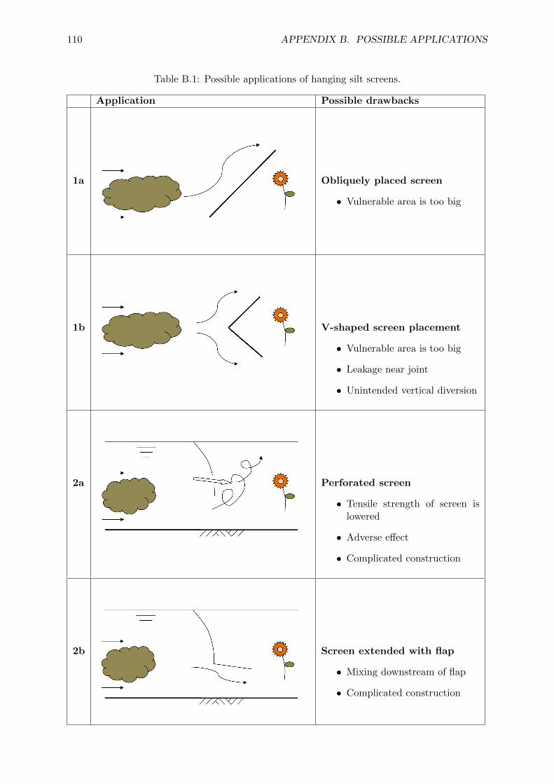
110 APPENDIX B. POSSIBLE APPLICATIONS
Table B.1: Possible applications of hanging silt screens.
Application Possible drawbacks
1a Obliquely placed screen
• Vulnerable area is too big
1b V-shaped screen placement
• Vulnerable area is too big
• Leakage near joint
• Unintended vertical diversion
2a Perforated screen
• Tensile strength of screen islowered
• Adverse effect
• Complicated construction
2b Screen extended with flap
• Mixing downstream of flap
• Complicated construction

111
Application Possible drawbacks
3a Gap between sections
• Concentrations not reducedsufficiently
3b Diffuser
• Concentrations not reducedsufficiently
• Complicated placement
4 Not achievable by means of a silt screen
5 Two silt screens
• Amount of silt screens dou-bled

112 APPENDIX B. POSSIBLE APPLICATIONS

113
Appendix C
Turbulence
When looking at a detailed time series of flow velocity measurements, one might observe some-thing like figure C.1. Above a certain combination of flow parameters rapid velocity fluctuationsoccur. This is the result of turbulence. It has been defined by Hinze (1975) as follows: ‘Tur-bulent fluid motion is an irregular condition of flow in which the various quantities show arandom variation with time and space coordinates, so that statistically distinct average valuescan be discerned’. Turbulence is characterized by three-dimensional flow structures of differentlength scales with a high degree of vorticity. At some point they are generated, then move onwith the flow while developing further and eventually die out. This process is visualized clearlyby for example smoke, whirling its way up through the air.
C.1 The onset of turbulence
The Reynolds number is a measure for turbulence. It represents the ratio of inertia over viscos-ity. This ratio can be used to illustrate the onset of turbulence. Panel 1 of figure C.2 depictsan initially laminar flow. Three streamlines lie nicely parallel to each other, but due to somereason left out of consideration a velocity difference appears. From Bernoulli’s law it followsthat pressure decreases between contracting streamlines, whereas it increases between diverg-ing streamlines. Panel 2 shows that the pressure difference leads to curvature of the middlestreamline, followed by an additional centrifugal force working in the same direction. Viscositycounteracts that process. Only when viscous forces are able to withstand inertial forces, thesedisturbances can be eliminated. This is generally the case for low flow velocities, small lengthscales, small fluid density and/or high viscosity. The flow is then said to be laminar. If not,the disturbances enhance themselves as illustrated in panel 3 and 4. One can imagine that thisleads to the development of three-dimensional flow structures.
Via this generation of turbulence, energy is transferred from the mean motion to the turbu-lent motion. The principle of figure C.2 is valid in a range of different length scales. Thereforeturbulent structures will be present from the biggest scales in a certain flow situation onto verysmall scales. Only at the smallest scales velocity gradients are high enough to allow for viscousdissipation of kinetic energy into heat. Turbulence can thus be seen as an intermediate stagein the dissipation of energy. The process of big whorls breaking down into ever smaller whorlsuntil dissipation comes into play is known as the energy cascade. It has been mentioned beforethat the degree of turbulence can be expressed by means of the Reynolds number. It was saidto represent the ratio of inertia over viscosity. Equation C.1 shows this in a parametrical way.
Re =Inertia
Viscosity=ρULµ
=ULµ/ρ
=ULν
(C.1)
When Re is less than about 2,300 the flow can be characterized as laminar. In case Re is higherthan about 4,000 the flow becomes turbulent. All values in between belong to the transitional

114 APPENDIX C. TURBULENCE
Figure C.1: Turbulent time series from research by Kang et al. (2003).
Figure C.2: Four successive stages in the onset of turbulence.

C.2. TYPES OF TURBULENCE 115
zone. The behaviour of the flow in this transitional zone can be explained by referring tofigure C.2. An initial disturbance as displayed in panel 1 is needed to get the generation ofturbulence going. Small disturbances can still be eliminated in the transitional zone, but biggerones develop into fully turbulent structures. The flow then obtains a variable state, with suddenoutbreaks of turbulence and periods of calm, laminar flow. Above Reynolds numbers of 4,000,disturbances continuously create new turbulent structures. The flow then really can be identifiedas turbulent.
The Reynolds number tells something about the character of a certain flow situation. Itdoes not specify anything about the spatial distribution of turbulence within that situation. Thestatistical description of turbulence offers a solution. In the time series of figure C.1, the thickred line indicates the mean value of all measured velocities. The complete signal u is thought tobe the sum of the mean velocity u and a fluctuating component u′. This is called the Reynoldsdecomposition. The dotted red lines mark the bandwidth of velocities within one standarddeviation (σ) of u. For a Gaussian distributed signal, this σ is equal to the root-mean-squarevalue of all turbulent fluctuations. The latter can be used as a typical order of magnitude,called the turbulence intensity r. The square of σ is the variance of all velocity fluctuations. Itis a measure of the kinetic energy contained in turbulent motions. Such velocity measurementscan be obtained everywhere in the flow. In that way the spatial distribution of turbulence canbe assessed.
C.2 Types of turbulence
Theoretically it is possible to generate laminar flow of any desired Reynolds number, as longas no disturbances are generated. In a laboratory situation one can create flows along verysmooth surfaces and with a minimum amount of internal shear. In that case flow is able toremain laminar up to fairly high Reynolds numbers. In hydraulic engineering practice however,sufficiently disturbing elements will always be present and the above-mentioned limits for Reare respected. Only one feature is responsible for the generation of turbulence, being a velocitygradient. Velocity gradients can have two different causes. This accordingly divides turbulentflows into two main categories: wall flow and free flow.
The term wall flow relates to flows that are governed by the proximity of a closed bound-ary. Viscosity prescribes a no-slip condition at the boundary surface. In case of a current,flow velocities away from the wall are non-zero. This will always result in a velocity gradientperpendicular to the wall. When a certain flow condition holds long enough, a boundary layerwill develop. In the boundary layer the influence of the wall is noticeable and flow velocitiesget higher with increasing distance from the wall.
Remote from a closed boundary, one speaks of free flow. Velocity gradients and the associ-ated generation of turbulence can still occur. Mixing layers, jets and wakes are identified as thethree main types of free turbulence. Grid turbulence and plumes might also be named in thisrespect. Grids are used in laboratory situations to create more or less homogeneous turbulence.Plumes form a somewhat separate category, since they are driven by density differences. Mostfree flows are characterized by self similarity. Velocity profiles perpendicular to the mean flowdirection at varying distance from the source of free turbulence are of the same shape.
An initial wall flow can transform into free flow. This process is known as flow separation.It occurs near sudden geometrical changes, like man-made structures or bedforms. The mainflow is then not able to follow the curvature of the boundary. When the cross-sectional widthincreases, continuity forces the flow to slow down. Near the boundary flow velocities are alreadyvery small. Therefore a negative velocity gradient in the direction of the mean flow can easilygive rise to negative velocities in that region. Hence a recirculation zone exists downstreamof the separation point. Between the main flow and the recirculation zone transverse velocitygradients are big. There a mixing layer develops with high turbulence intensities. At some

116 APPENDIX C. TURBULENCE
Figure C.3: Typical shape of the one-dimensional energy-density spectrum of a turbulent flow.
distance downstream of the disturbance, flow recovery takes place. A new boundary layergradually develops based on the downstream geometry.
C.3 Turbulent kinetic energy
It was already briefly mentioned that the generation of turbulence transfers energy from themean flow to the turbulent fluctuations, which eventually leads to dissipation. The energy of aturbulent flow is distributed over the mean flow and the turbulent motions. This becomes clearafter applying the Reynolds decomposition to the total energy of the flow per unit volume, seeequation C.2.
E =1
2ρuu =
1
2ρuu︸ ︷︷ ︸Em
+1
2ρu′u′︸ ︷︷ ︸Et
(C.2)
As energy is passed on from large to small scales, it is interesting to analyse how the turbulentkinetic energy (TKE) Et is distributed over the length scales. A turbulent timeseries can be seenas the sum of the signals of all passing eddies. Therefore, all length scales of the turbulent flowshould be represented in it. However, a single-point timeseries merely contains information ontime scales and not on length scales. To make the conversion, an assumption is needed aboutthe way turbulent structures travel through the space domain. This assumption is providedby Taylor’s hypothesis, also known as the frozen turbulence approximation. It states that thevelocity field, being a collection of ‘frozen’ turbulent eddies, translates through the space domainat constant velocity. When considering a single-point timeseries, the frozen velocity field travelsalong the local streamline at mean velocity. Therefore, projecting the velocity componentsonto the streamline and multiplying the sample times with the mean velocity results in anapproximation of the spatial distribution of velocities along the streamline. Due to the couplingbetween the time and space domains the spatial coordinates are reversed, but this does notaffect the analysis.
By taking the Fourier transform of the autocovariance of the converted turbulent timeseriesand integrating over the three dimensional wavenumber space, the one-dimensional energy-density spectrum is obtained. Typically the spectrum is shaped like the solid line in figureC.3. The left-hand side of the figure represents the large, energy containing eddies. The right-hand side represents the length scales at which dissipation takes place. The part in between,

C.3. TURBULENT KINETIC ENERGY 117
commonly known as the inertial subrange, contains the energy cascade. Based on dimensional
considerations, energy-density can be shown to scale with k−5/3w in the inertial subrange.

118 APPENDIX C. TURBULENCE

119
Appendix D
Fine sediment
Fine sediments form a separate part of sediment theory. They are mainly distinguished by smallparticle sizes and accordingly small weights. Nevertheless, chemical aspects turn out to be atleast as important. Section D.1 discusses the basic properties of fine sediment. In section D.2erosion, transport and deposition of fines are addressed. Finally section D.3 clarifies similaritiesand differences between SSC and turbidity. An elaborate description of fine sediment dynamicsis found in e.g. Whitehouse et al. (2000), on which this appendix is largely based.
D.1 Properties of fine sediment
All particles with an equivalent diameter d smaller than 63 mm are classified as fine sediment.Within this category an important difference exists between silt and clay. This difference ischaracterized by particle size as well as particle nature. Particles having a diameter between 2and 63 mm are officially recognized as silt. Smaller ones are said to be clay particles. Althoughthese limits are roughly adhered to, the most decisive aspect is particle nature. Silt particlesare comprised of quartz minerals, just like sand. Therefore, silt can simply be thought to act assand grains with very small particle diameters. Clay however consists of clay minerals (primarilykaolinite, illite, chlorite and montmorillonite). Because of their specific properties, clay mineralsmainly form a plate-like structure. These clay particles are much less stable than silt grains ina chemical sense.
One of the most relevant parameters of sediment regarding morphologic research is its set-tling velocity ws. Sediment particles are suspended in the surrounding water instead of dissolved.Besides flow-related and chemical forces, gravity is the most important force acting on a par-ticle. When releasing a particle in stagnant water, its fall velocity will reach a constant valueafter an initial start-up phase. This is due to a balance between gravity and the drag force.The drag force FD acting on a falling particle depends on the flow characteristics. For smallReynolds numbers Re = wsd/ν, viscosity dominates inertia. This generally holds for fallingfine sediment particles in water. In that case, Stokes’ Law is applicable and FD is calculatedaccording to equation D.1. Particles are schematised as spheres.
FD = 3πµdws (D.1)
The gravitational force acting on a submerged spherical particle of density ρs and volume V isgiven in equation D.2. When drag force and gravitational force Fg have reached a balance, thefinal fall velocity ws∞ follows from equation D.3.
Fg = (ρs − ρ)gVp = (ρs − ρ)g1
6πd3 (D.2)

120 APPENDIX D. FINE SEDIMENT
FD = Fg
3πµdws∞ = (ρs − ρ)g1
6πd3 (D.3)
ws∞ =(ρs − ρ)gd2
18µ
Final fall velocities are always relatively small. The acceleration phase is very brief and theequilibrium situation is reached quickly. As a result, ws∞ will simply be indicated as ws. Set-tling velocities of fine sediment are in the order of 0.01 mm/s, whereas coarser ones typicallyhave settling velocities in the order of 1 cm/s. This leads to an important difference of be-haviour between both types. For water depths in the order of 10 m, settling times of fine andcoarse particles are 106 s and 103 s respectively. The settling velocity of fine sediment is easilyoverruled by an upward vertical flow velocity, increasing settling times even further. The moreor less floating behaviour of fines elucidates the troubles faced fighting turbidity.
It was already mentioned briefly that clay is less stable than silt in a chemical sense. The plate-like clay particles formed by clay minerals possess ionic charges. Their edges are positivelycharged, their faces negatively. Other charged particles can get attracted by these electrostaticforces. Water might contain free cations (positively charged) and anions (negatively charged).When clay gets in touch with water, cations form a layer on the plate faces and anions collectaround the edges. The charged clouds surrounding clay particles are able to cling together.Organic material can be adsorbed as well. Long polymer chains offer an effective way of gath-ering particles together in flocs. Hence the process is called flocculation. Big empty spaces inthese aggregates are filled with water, giving flocs a water content of 90 to 98% under naturalconditions.
Flocs are formed due to attractive forces. However, the magnitude of these forces decreasesrapidly with distance. Therefore particles have to be brought into contact with each otherin order to achieve cohesion. The processes of collision and cohesion are therefore the mostimportant ones regarding flocculation. Cohesion has been discussed above. Collisions betweenparticles can have three different causes: Brownian motion, internal shear and different settlingvelocities. From analogy with diffusion, it becomes clear that Brownian motion is only able tocause collision of particles on a small scale. The range of different settling velocities depends onthe chemical and biological characteristics of water and sediment. Internal shear plays a dualrole. It is both a floc promoting and limiting process. Turbulence comes with internal shear.When turbulence intensities are high enough, aggregates start disintegrating again.
Flocculation is not just an interesting side effect of clay. It influences the physical parametersregarding suspended sediment to a great extent. Due to the large water content of flocs, theirdensity ρf decreases to about 1100 kg/m3. The equivalent diameter of a floc may vary frommicrons to millimeters. The increase of d tends to have a bigger influence on ws than thedecrease of ρf . Therefore flocculation is able to magnify settling velocities drastically.
In a natural environment, fine sediment will virtually never consist of only one type. Clay, siltand sand particles are found mixed up in varying proportions, together with organic material,water and sometimes gas. The mixture is mostly indicated as ‘mud’. The clay content andchemical properties of the surrounding water determine whether sediment is cohesive or not.
Whether or not cohesive, one single value of the settling velocity will never be applicableto every particle in a specific situation. Grains and flocs coexist in a variety of sizes, eachwith its own settling velocity. Therefore it comes down to a settling velocity distribution. Fornon-cohesive sediment in low suspended concentrations, settling velocities are readily linkedto the grain size distribution. In case of cohesive sediment, the composition of flocs may varysignificantly. The Stokesian settling velocity according to equation D.3 does not hold, since flocscan not be schematised as homogeneous spheres. Various authors have reported on cohesive

D.1. PROPERTIES OF FINE SEDIMENT 121
Figure D.1: Experimental data relating the settling velocity of mud flocs to the suspendedsediment concentration (Winterwerp, 1999).
settling velocity distributions. At low concentrations, a very simple relation like equation D.4may be used, but with caution.
ws50 = kCm (D.4)
Here ws50 denotes the median settling velocity, i.e. the settling velocity exceeded by 50% of allflocs, C is the suspended sediment mass concentration and k and m are coefficients. Whitehouseet al. (2000) propose k = 0.001 and m = 1.0. Low concentrations are defined as lower than 3000mg/l. Winterwerp (1999) expanded equation D.3 to calculate the settling velocity of individualmud flocs. This resulted in equation D.5.
ws,r =α
18β
(ρs − ρw)g
µD
3−nfp
Dnf−1
1 + 0.15Re0.687p
(D.5)
Here, α, β and nf are coefficients depending on the shape of the floc, Dp is the diameterof primary mud particles, D is the floc diameter and Rep = ws,rD/ν is the particle Reynoldsnumber. The left-hand side of figure D.1 shows the relation between settling velocity of mud flocsand suspended sediment concentration for various experimental datasets. The line indicating a1-in-1 slope represents equation D.4 with k = 0.001 (note the unit mm/s on the vertical axis)and m = 1.0. It appears that especially coefficient k varies from case to case.
The right-hand side of figure D.1 shows the process of hindered settling. At high suspendedsediment concentrations, settling flocs interfere with each other and the surrounding flow offluid. This reduces the settling velocity, which is expressed by the decaying line at the right-hand side of figure D.1. Winterwerp (1999) distinguishes seven processes affecting the settlingvelocity of individual particles in a suspension:
• A falling particle of finite dimensions gives rise to return flow and wake formation. Sur-rounding particles are slowed down by the return flow, but accelerated when pulled intothe wake.

122 APPENDIX D. FINE SEDIMENT
• Return flow and wake formation involve velocity gradients. This dynamic or flow effectleads to a change in pressure distribution, added mass of the particles and hydrodynamicdrag.
• Particle-particle collisions lead to a direct exchange of momentum between particles. Ascollisions lead to a loss of energy, on average particles are slowed down.
• Particle-particle interactions are the combined effect of attracting and repelling forcesbetween particles due to e.g. electrical charges.
• The presence of particles in a fluid leads to an increase of viscosity. As individual particlesare thought to fall in the surrounding suspension, their settling velocity is decreased.
• The argument that individual particles fall in the surrounding suspension can be used aswell to discuss the increase of density of the fluid. Individual particles are slowed downby their higher buoyancy.
• When a particles are pulled into the wake of another particle, this might induce cloudformation. The cloud starts to behave as a large grain, which leads to an increase ofsettling velocity.
The onset of hindered settling happens above concentrations of 1 g/l, which is the upper limit ofconcentrations measured near silt screens. However, closer to the source of turbidity, hinderedsettling will come into play.
D.2 Erosion, deposition and transport
The real importance of (fine) sediment to hydraulic engineers is its ability to get transportedby a current. Or to put it different: its impotence to remain in position. Above a certain limitof flow parameters, sediment gets eroded from the bed. It is then transported by the current.Under influence of its settling velocity, every particle is deposited back onto the bed eventually.Three consecutive subsections address the processes of erosion, deposition and transport.
D.2.1 Erosion
Equations for erosion of cohesive beds are mostly based on the threshold bed shear-stress τe.The value of τe is related to some parameter representing bed density. Either bulk-densityρB = mass of mixture/volume of mixture or bed-concentration Cb = mass of grains/volume ofmixture is used for this purpose. The formulation of Thorn and Parsons is commonly used andis given in the empirical equation D.6.
τe = E1CE2b (D.6)
E1 and E2 are dimensional coefficients. Their values are subject to debate and may vary slightlyfrom situation to situation. Whitehouse et al. (2000) state that the values E1 = 0.0012 andE2 = 1.2 give the best fit in general (with Cb in g/m3).
Based on τe, the empirical equation D.7 by Partheniades is applicable to compute the rateof erosion dm/dt. The rate of erosion denotes the dry mass of cohesive sediment eroded perunit area per unit time.
dm
dt= Me(
τ0τe− 1) for τ0 > τe
dm
dt= 0 for τ0 ≤ τe (D.7)

D.2. EROSION, DEPOSITION AND TRANSPORT 123
Dimensional coefficient Me is known as the erosion rate. From literature study, Van Rijn(2005) reports values between 10−5 and 5 ·10−4 kg/(sm2), depending amongst others on mineralcomposition, organic material and salinity. τ0 is the bed shear-stress and the term (τ0/τe − 1)is called the relative excess bed shear-stress.
D.2.2 Deposition
Due to the settling velocity, suspended particles tend to return to the bed. Therefore the mainparameter regarding deposition is the median settling velocity ws50. In case of still water, thereis no sediment movement but settling. The rate of deposition dm/dt then depends solely onws50 and C0. The latter denotes the near-bed concentration of suspended sediment. EquationD.8 shows this relation.
dm
dt= −C0ws50 (D.8)
In case of flowing water, the above equation needs modification. Increasing bed shear stress willdecrease the deposition flux. Whitehouse et al. (2000) proposes to use a threshold bed shear-stress for deposition τd, above which deposition completely ceases. In mathematical terms thisrelationship is expressed by equation D.9.
dm
dt= −(1− τ0
τd)C0ws50 for τ0 < τd
dm
dt= 0 for τ0 ≥ τd (D.9)
The notion of one threshold bed shear-stress for deposition does only hold under assumption ofhomogeneous suspended sediment. For varying grain or floc sizes, every particle has got its ownvalue of τd. When used in combination with the median settling velocity ws50, values between0.06 and 0.10 Nm-2 are suggested for τd by Whitehouse et al. (2000).
Winterwerp (2003) argues that a threshold bed shear-stress for deposition does not exist.He considers it an apparent effect resulting from a threshold bed shear-stress for resuspensionof deposited material. In this research, these findings are incorporated by assigning an infinitelyhigh value to τd.
Furthermore it is possible to introduce sediment fractions. The total collection of particlesis broken down into discrete fractions, each with its own τd, ws and C0. Calculation of the rateof deposition is done per fraction. Summation over all fractions gives the total deposition flux.
D.2.3 Transport
Transport of suspended sediment can be explained best by setting up a mass balance. Thisexercise is closely related to the basic equations governing two- and three-dimensional flow andtransport models. Therefore it is discussed in the corresponding section on basic equations inappendix F. For now the treatment of theory on suspended sediment transport is restricted toa couple of important notions.
Generally, transport of suspended sediment is simplified to transport of a passive tracer withan additional vertical velocity due to settling. On the whole, three different processes can berecognised: advection, diffusion and dispersion. The latter term is sometimes used ambiguouslyin fluid mechanics. Here, dispersion indicates the direct effect of velocity gradients in the meanmotion on a cloud of suspended material. Different parts of the cloud are advected at differentvelocities. As a result, the cloud starts deforming. It should be noted that dispersion onlychanges the shape of the cloud, while the volume remains the same. Therefore dispersion doesnot influence concentrations directly, although it is able to increase the surface area subjectedto diffusion. Depending on the boundary conditions, spreading can be governed by differentprocesses.

124 APPENDIX D. FINE SEDIMENT
As we have seen already, cohesive sediment brings along some complications regarding set-tling velocity. As expressed in equation D.4, the median settling velocity depends on the con-centration of suspended sediment rather than grain size. In general, concentrations vary invertical direction. Hence the settling velocity of cohesive sediment varies in vertical directionas well. Closer to the bed, concentrations are higher. This leads to a higher settling velocity.The opposite is valid closer to the free surface.
D.3 Turbidity
The terms suspended sediment concentrations (SSC) and turbidity have been used interchange-ably. They are closely related indeed. In fact SSC and turbidity are different measures for thesame phenomenon. The use of suspended sediment concentrations is very straightforward. It isequal to the weight of all suspended sediment particles present in a predefined volume of water.This is an exact measure, although it requires some steps to determine SSC given a certainvolume of water.
Turbidity, in the context of dredging operations, is concerned with the presence of suspendedsediment particles in water as well. As the international standard NEN-EN-ISO 7027 (2000)defines it, turbidity is a reduction of transparency of a liquid caused by the presence of undis-solved matter. Hence, it focuses on visual aspects rather than exactly measurable quantities.Two units are commonly used to express turbidity, being the Nephelometric Turbidity Unit(NTU) and Jackson Turbidity Unit (JTU). The former is used in this report. Its measurementis based on the amount of reflection of a light beam pointed at the suspension. The use ofNTU does not belong to exact science, since a direct link to SSC can not be made. NTU valuesdo not only vary with SSC, but also with shape, reflective properties and colour of sedimentparticles. Despite this disadvantage compared to SSC, turbidity is still commonly used as aquantity in hydraulic engineering because of the simplicity of measurements. These can simplybe carried out by means of a so-called nephelometer. Nevertheless, one should always be awareof the shortcomings.

125
Appendix E
Laser Doppler Anemometry
Local velocities were said to be measured by means of Laser Doppler Anemometry (LDA). Thisis an optical measurement technique, which makes use of laser beams. The general applicationof the instrument is depicted in figure E.1. A single laser beam passes through an acousto-opticmodulator (also known as a Bragg cell). By means of acoustic waves, the Bragg cell splits thelaser beam into two separate beams. These adopt the frequency of the acoustic waves, whichis far lower than the frequency of the electromagnetic laser frequency. The beams are focusedby means of a lens, so as to create an intersection of both beams within a fluid under an angleθ. Within the intersection, the beams create an interference pattern based on the Bragg cell’sacoustic frequency. The interference pattern is indicated in the bottom left corner of figure E.1.
Fine suspended particles within the fluid scatter the laser light when they pass through theintersecting beams. The scattered light, which has attained a Doppler shift with respect tothe issuing light, is recorded by a receiver. The velocity can now be derived from this Dopplershift. This is done by means of figure E.2. The two green laser beams consist of successivecrests (black lines) and troughs. It is readily seen that the crests intersect along straight lines,called fringes. The Doppler frequency, that is the difference between the issuing and recordedfrequencies, modulates the amplitude of the recorded signal. When a particle moves through afringe it scatters a high light intensity and in between fringes it scatters a low light intensity.When the fringe spacing δ is known, the velocity of the particle can be calculated from theDoppler shift of the scattered signal. The fringe spacing depends on the wave length λ of thelaser beams. It is derived by means of the right-hand side of figure E.2. First, λ and δ aredefined:
AF = EB = λ
DC = δ
The crests are directed perpendicular to the direction of propagation. This yields:
∠ACB = θ
Triangle ABC is an isosceles triangle and AF, BE and CD are its altitudes. Four similar trianglescan be discerned:
4ACD ∼ 4BCD ∼ 4ABE ∼ 4BAF
Due to similarity of triangle ABE and triangle ACD, angle ABE is found:
∠ABE = ∠ACD = θ/2

126 APPENDIX E. LASER DOPPLER ANEMOMETRY
Figure E.1: The working principle of LDA (http://www.dantecdynamics.com/).
Figure E.2: The interference pattern of two crossing laser beams.

127
With the help of some trigonometry, δ can be expressed in terms of λ and θ:
AB =AF
cos θ/2=
λ
cos θ/2= 2AD = 2CD tan θ/2 = 2δ
sin θ/2
cos θ/2
δ =λ
2 sin θ/2
Let the recorded Doppler frequency be fD. Now the particle’s velocity u can be calculated:
u = fDδ
However, the sign of u can still not be determined. Irrespective of which way the particlemoves through the fringes, the recorded Doppler shift will be the same. Therefore, the frequencyof one of both laser beams is given a small, known shift fs. This causes the fringes to moveslowly at a speed vs, which equals:
vs = fsδ
Now the recorded amplitude modulation has got a frequency of fs + fD or fs− fD, which takesaway the directional ambiguity.

128 APPENDIX E. LASER DOPPLER ANEMOMETRY

129
Appendix F
Numerical models
For this research, use is made of two computational fluid dynamics (CFD) models. The fully3-dimensional Large Eddy Simulation code Dflow3D is used to investigate the process of verticaldiversion. The 2-dimensional horizontal (2DH) code FINEL2D is applied to study horizontaldiversion. Section F.1 will deal with the basic equations governing flow and transport. Afterthat, section F.2 presents the specifics of Dflow3D and section F.3 treats those of FINEL2D.
F.1 Basic equations
Generally, incompressible 3-dimensional flows of a Newtonian fluid are described by means ofthe continuity equation and the incompressible Navier-Stokes equation. The former is presentedby equation F.1 and follows from a mass balance.
∂ρ
∂t+∇ · (ρu) = 0 (F.1)
The continuity equation implies that the velocity field is free of divergence. The incompressibleNavier-Stokes equations can be derived from the momentum balance and are presented byequation F.2.
∂ρu
∂t+∇ · (ρuu) = −∇p+∇ · τ + ρF (F.2)
Here, u denotes the 3-dimensional velocity vector, p is pressure, τ is a shear stress tensor andall body forces like Coriolis and gravity are lumped in F.
Transport of suspended solids is can be described by means of a transport equation for(volume) concentration Cv. This is given in equation F.3.
∂Cv∂t
+∇ · (uCv) = ∇ · (D∇Cv) (F.3)
In this equation, D is the diffusion coefficient.
Turbulent fluctuations occur down to very small length scales. Solving for all these length scalesand their associated time scales in a CFD model is known as direct numerical simulation (DNS).These are computationally very expensive, which limits the domain size to a large extent. Asolution is found in applying the Reynolds decomposition to the Navier-Stokes equation. Thenon-linear advection term creates an extra term stemming from the fluctuating velocity com-ponent. Equation F.4 shows the resulting Reynolds-averaged Navier-Stokes (RANS) equation.
∂ρu
∂t+∇ · (ρuu) +∇ · τ ′ = −∇p+∇ · τ + ρF (F.4)
with τ ′ = ρu′u′

130 APPENDIX F. NUMERICAL MODELS
The extra term represents the gradient of the so-called Reynolds stresses or turbulent shearstresses τ ′. These still contain the fluctuating velocity component and require simplificationin order to speed up numerical simulation. Methods to close the Navier-Stokes equations areknown as turbulence models. Many turbulence models focus on finding an expression for theReynolds stresses based on the averaged velocity vector, but different and more sophisticatedmodels exist as well.
F.2 Dflow3D
Dflow3D is an academical CFD model optimised for the use of Large Eddy Simulation (LES).It is a rigid lid model, meaning that the model has a constant depth instead of a free surface.LES is a turbulence model which makes use of averaging in space instead of averaging in time.The bigger length scales of the turbulent energy-density spectrum contain the anisotropic partof all turbulent fluctuations and are therefore responsible for most of the shortcomings of time-averaged turbulence models. In LES, turbulent length scales are represented down to the gridcell size. The more isotropic part of the energy spectrum is filtered out of the equations byfiltering over one or more grid cells. In the inertial range, the key function of smaller lengthscales is extracting energy from the bigger length scales in order to keep the energy cascadegoing. This process can be approximated quite well by means of a sub-grid scale (SGS) stressterm. The resulting filtered equation looks much like the RANS equation, except for the factthat the overbars represent averaging in space and the Reynolds stresses have been replaced bythe sub-grid stress τsgs, see equation F.5.
∂ρu
∂t+∇ · (ρuu) = −∇p+∇ · τ +∇ · τsgs + ρF (F.5)
An additional model is now needed to compute τsgs. In this study, the wall-adapting localeddy-viscosity (WALE) model is used (Nicoud and Ducros, 1999) with a WALE constant Cw of0.325.
Transport of suspended solids is computed by means of equation F.3. D is determined fromthe kinematic viscosity as D = ν/Sc, where Sc is the Schmidt number. The kinematic viscosityused in Dflow3D is the sum of the molecular kinematic viscosity and the SGS kinematic viscositycomputed by the WALE model. The value of Sc is discussed further in chapter 4.
F.3 FINEL2D
FINEL2D is a 2DH CFD model based on the shallow water equations. If the horizontal lengthscales of a flow are much bigger than the vertical length scales, vertical accelerations may be as-sumed to equal zero. This leads to a hydrostatic pressure distribution. Integrating the continuityequation and Navier Stokes equation over depth and applying the Boussinesq approximationregarding buoyancy results in equations F.6 and F.7 respectively.
∂η
∂t+∇ · (hU) = 0 (F.6)
Here, h = η+ zb denotes the actual water depth with η the surface elevation and zb the verticalbed coordinate, and U is the two-dimensional depth-averaged velocity vector.
∂hU
∂t+∇ · (hUU) + gh∇η − 1
ρτb = 0 (F.7)
Bed shear stress is represented by the vector τb. It should be noted that turbulent shear stressesare left out of consideration in FINEL2D. This restricts the use of the code to flows dominatedby advection.

131
Appendix G
Validation figures
Validation of the CFD model Dflow3D is done by means of the laboratory experiments conductedfor this research. An elaborate description of validation scenario 2A is given in section 4.2.2.This appendix contains figures for all scenario’s.

132 APPENDIX G. VALIDATION FIGURES
Figure G.1: Validation of the numerical model for laboratory scenario 1A.

133
Figure G.2: Validation of the numerical model for laboratory scenario 1B.

134 APPENDIX G. VALIDATION FIGURES
Figure G.3: Validation of the numerical model for laboratory scenario 2A.

135
Figure G.4: Validation of the numerical model for laboratory scenario 2B.

136 APPENDIX G. VALIDATION FIGURES
Figure G.5: Validation of the numerical model for laboratory scenario 3A.

137
Figure G.6: Validation of the numerical model for laboratory scenario 3B.

138 APPENDIX G. VALIDATION FIGURES

139
Appendix H
Effectiveness figures
In this appendix, plots of Ein(6h) and Eref (6h) are presented together with the actual datapoints.
Figure H.1: Inflow effectiveness Ein(6h) for profile U1 (%).
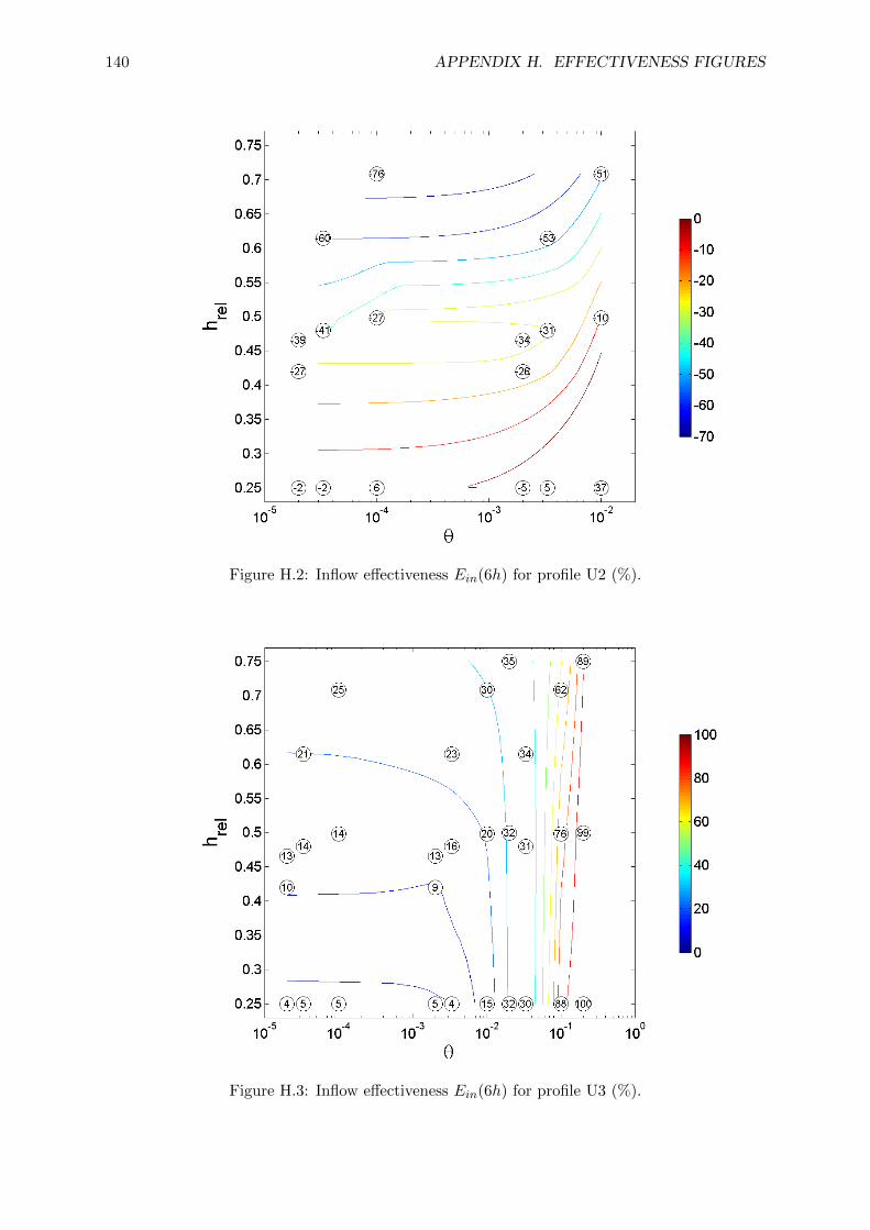
140 APPENDIX H. EFFECTIVENESS FIGURES
Figure H.2: Inflow effectiveness Ein(6h) for profile U2 (%).
Figure H.3: Inflow effectiveness Ein(6h) for profile U3 (%).

141
Figure H.4: Reference effectiveness Eref (6h) for profile U1 (%).
Figure H.5: Reference effectiveness Eref (6h) for profile U3 (%).

142 APPENDIX H. EFFECTIVENESS FIGURES

143
Appendix I
Case studies revisited
Appendix A treated a couple of case studies regarding silt screen effectiveness, stemming fromboth internal research by dredging company Boskalis as well as published research by Vu et al.(2010) and Jin et al. (2003). The case studies and the associated conclusions are now re-examined, bearing in mind the knowledge gained from this research.
I.1 Experiments by Boskalis
Boskalis conducted three field measurements regarding silt screens of the hanging type. Theirspecifications are recalled in table I.1.
Table I.1: Specifications of silt screen field experiments by Boskalis.
Case 1 Case 2 Case 3
Geometry Open water Semi-enclosed reclamation Semi-enclosed reclamation
h 13.5 m 9 m 6 m
hrel 0.5 0.66 1
W∗ 20 54 25
U 0.1 m/s very small very small
Conclusions Negative Neutral Positive
Neutral conclusions were drawn on silt screen effectiveness in case 2, as no dredging-inducedturbidity reached the screen. This observation is endorsed here, so case 2 is left out of furtherconsideration.
Case 1 deals with a linear silt screen at open water, which is therefore susceptible to horizontalas well as vertical diversion. Both processes are recognised by the authors during the passageof an overflow plume. Figure I.1 shows three consecutive phases of this event. In the leftpanel the plume is mainly located upstream (to the left of the screen). The last few metersupstream show a fairly clear free surface, indicating that the sediment-laden main flow is di-verted vertically. Downstream of the screen some turbidity has already been mixed into therecirculation zone, judging from the moderately turbid free surface. The middle panel showsthe screen being surrounded by turbidity as a result of horizontal and vertical diversion. Fi-nally, the left panel proves the existence of a downstream recirculation zone. After the mainpart of the plume has moved out of sight, significant suspended sediment concentrations persistimmediately downstream of the silt screen.
Turbidity was measured at several depths while sailing circles around the screen with asurvey vessel. Around 75 m upstream of the screen, turbidity values range from 5 NTU near

144 APPENDIX I. CASE STUDIES REVISITED
Figure I.1: Three consecutive images of an overflow plume passing a hanging silt screen (at t =11:11, 11:24 and 12:25). Courtesy Boskalis.
the free surface to 30 NTU near the bed. This is in fair agreement with profile L1 or E1 as usedin this research. At 25 m downstream of the screen, a more or less uniform turbidity profile isfound with values between 10 and 15 NTU. The following conclusions are drawn by the authors:
- A silt screen at deep water, placed perpendicular to the main current with a relative screenheight of 0.5 is not an effective measure to mitigate dredging induced turbidity.
- The silt screen causes additional stirring of fine sediment into the water column, whichincreases plume decay times.
- Successful application of silt screens at deep water demands at least (1) increased screenheight to block a larger part of the water column and (2) extended screen width to covera wider variety of flow directions.
- As the adaptations proposed above might not be feasible, it is recommended to focus effortson the development of operational measures to minimise the release of fine sedimentstogether with sound skills for plume prediction.
Although the effectiveness of the screen is correctly judged, a number of remarks can be maderegarding these conclusions:
• The big water depth is mentioned indirectly as a factor which negatively influences siltscreen performance. This research has proved that the influence of water depth on siltscreen effectiveness is negligible. However, the authors might implicitly associate a smallerwater depth with smaller flow velocities and the presence of land masses which preventhorizontal diversion. Although that would at least improve the inflow effectiveness in arelative sense, a truly effective hanging silt screen does not exist.
• Increasing the (relative) height of the silt screen does not lead to effective mitigation of sus-pended sediment. It only induces more horizontal diversion and more intense downstreammixing.
• Increasing the screen width is suggested as way of preventing excessive horizontal diver-sion. It is true that increasing W∗ leads to a bigger relative discharge, but this effect islimited (see figure 5.5). Within the range of realistic W∗, the part of incoming dischargebeing diverted vertically will never get much higher than 50%.
Case 3 concerns the application of a hanging silt screen just outside the open end of a semi-enclosed reclamation. Turbidity is caused by a cutter suction dredger pumping dredged materialinto the reclamation through a pipeline. This causes high suspended sediment concentrationson the inner side of the screen, ranging from several 100 to 1000 mg/l. The authors assume the

I.2. CASE STUDIES IN LITERATURE 145
existence of near-bed turbidity currents, since the sheltered environment is expected to havevirtually no mixing. The associated high Richardson number allows for stable stratification.Turbidity values measured on the outer side of the screen are 4 to 8 times lower than those onthe inner side, which leads the authors to the following conclusions:
- Systematic variation of mid-depth turbidity values with the tidal level confirm the oc-currence of density-driven currents. A sudden increase of turbidity is observed when thesensor touches the dense layer.
- The strong decrease of measured turbidity values from the inner to the outer side of thesilt screen shows that the screen effectively blocks part of the fine sediment present in thedense layer.
- This decrease can not be fully attributed to the presence of a silt screen, as a turbiditycurrent would show a certain degree of settling anyway.
- Effective functioning of the silt screen finds further confirmation from the observation thatthe screen, by the time that it was pulled out, was partly buried under a layer of sediment.
The following remarks have to be made regarding these conclusions:
• The high effectiveness of the silt screen can largely be attributed to it’s coverage of theentire water column. The screen is partly buried under a layer of sediment, which meansthat its lower edge touches the bed. This puts the screen out of the scope of this research,as it does not allow for vertical diversion. Such a configuration is only feasible in veryweak cross currents.
• Burial of the screen’s lower edge might cause trouble during removal. The typical advan-tage of hanging silt screens over standing screens, being the absence of the need for heavyfloating equipment, does not hold in this case.
I.2 Case studies in literature
In literature, two case studies of silt screen effectiveness were encountered. Their relevant pa-rameters are summarised in table I.2.
Table I.2: Specifications of silt screen case studies encountered in literature.
Jin et al. (2003) Vu et al. (2010)
Geometry Open water Open water
h 5.5 m 22.5 m
hrel 0.6 0.5
W∗ 80 18
U 0.2− 0.3 m/s 0.3− 0.6 m/s
Conclusions Negative Positive
Jin et al. (2003) investigated the effectiveness of a hanging silt screen at open water. Tur-bidity was caused by three mechanical dredgers, operating at 220 to 330 m from the silt screen.Ebb-tidal currents are directed from the dredging site perpendicularly to the screen. An ex-tensive measurement campaign is conducted, see figure I.2. The six measurement locationsindicated by solid black dots numbered 1-1 to 2-3 are of special interest, as well as locations A1and A2. Vertical SSC profiles are obtained at paired locations upstream and downstream of the

146 APPENDIX I. CASE STUDIES REVISITED
Figure I.2: Overview of case study into silt screen effectiveness by Jin et al. (2003).
screen, represented by the solid black dots. During ebb-tidal current, virtually all measurementsshow that downstream SSC profiles exceed the upstream ones up to 100%. Upstream SSC val-ues mostly range from 5 mg/l near the free surface to 10 mg/l near the bed. At locations A1and A2, mid-depth values of flow velocity and SSC are obtained. It stands out that downstreamflow velocities are about half as high as the upstream values. This phenomenon systematicallyswitches along with the tidal current direction. Jin et al. (2003) conclude as follows:
- The flow velocity at 30 m downstream of the silt screen is about half that found at thesame distance upstream.
- Even for a relatively weak storm period, SSC increases up to the value caused by dredging.
- Depth-averaged SSC downstream of the screen is higher by 60% with respect to theupstream side. This contradicts the major purpose of the screen, which is to reduce SSC.
- Screen efficiency evaluated by the SSC flux at mid-depth is about 55%. Considering thehigher SSC downstream, however, depth-integrated flux downstream may be comparableto that upstream.
- Considering the above results, the silt screen of the fixed hanging type installed from thesurface to about half of the water depth does not confirm a mitigation measure against thespreading of suspended sediment plumes generated by dredging in the study area, wherethe mean flow velocity ranges from 20 to 30 cm/s.
The negative conclusions are confirmed here. However, a number of remarks should be made:
• Jin et al. (2003) completely ignore the presence of horizontal diversion. As the screenis applied at open water without any lateral restrictions, this process will definitely takeplace.
• The authors attribute the high reduction of flow velocity at mid-depth to the existence ofa near-bed jet flow and a recirculation zone above. However, the measurement location issituated at about 6 times the water depth downstream. This will probably be in the zone

I.2. CASE STUDIES IN LITERATURE 147
of flow recovery, where mid-depth flow velocities should at least equal the upstream valuesand might even be slightly higher. Instead, the reduced flow velocity can be explainedvery well by the presence of horizontal diversion, which leads to a decrease of specificdischarge by about 50%.
• The increase of depth-averaged SSC from upstream to downstream can be caused by anumber of different processes. First of all, a continuous upstream supply of suspendedsediment gives rise to turbulent diffusion into the recirculation zone, leading to an increaseof SSC in the upper part of the water column. However, it was mentioned before thatthe profiles are obtained downstream of the recirculation zone. Second, screen-inducederosion might be a source of suspended sediment downstream of the silt screen. Sedimentsamples indicate that the bed contains significant silt and clay fractions. Finally, it mightbe possible that measurements are conducted when the main part of a dredging spill hasalready passed by. Persistent turbidity in the recirculation zone might give rise to highdownstream SSC. Again it should be noted that measurements are conducted downstreamof the recirculation zone.
• The 55% decrease of SSC flux at mid-depth is explained by the authors as a local phe-nomenon. They expect depth-integrated fluxes to be equal on both sides of the screen.This would only hold when the situation can be schematised with a 2DV approach. Dueto horizontal diversion this is not the case. Additional sediment fluxes around the screen’sside edges will probably account for the remaining percentage.
The last case study was investigated by Vu et al. (2010). Again, the silt screen was deployedat open water. The water depth, flow velocity and screen dimensions are well outside theallowable ranges commonly encountered in literature. Suspended sediment is released by grabdredgers, operating at an unspecified distance from the silt screen. The tidal current is directedperpendicular to the screen.
At both sides, SSC and flow velocities are measured at 10, 20 and 30 m from the screen.When the current is directed from the dredging area towards the screen, significant reductions ofSSC and especially sediment flux are found at the downstream side, see figure I.3. The authorsadmit that knowledge on the hydrodynamic processes and sediment behaviour in the vicinityof the silt screen is lacking. Hence they draw no conclusions regarding silt screen effectivenessfor this case study. Nevertheless, a number of interesting remarks is made here:
• The observed reduction of SSC corresponds fairly well with results obtained in this re-search for inflow profile U1 (uniform over the entire water column). For discontinuousplumes with a relatively long inflow duration, a reduction of 18% near the free surface isplausible. Nevertheless, instantaneous SSC values alone do not represent the full storyregarding silt screen effectiveness. Both the conversion to environmental impact potentialand integration over time (for discontinuous plumes) should be carried out to provide amore complete picture.
• The reduction of SSC fluxes is open to various interpretations. The flux is computed asthe product of flow velocity, SSC and vertical bin height. It is corrected to account forthe angle between the incoming flow and the silt screen. A lower value downstream withrespect to upstream can be explained by a couple of different reasons, including horizontaldiversion and extensive settling. The latter is certainly not expected within 10 m upstreamand downstream of the silt screen. Although it is questionable as well whether high lateralfluxes of sediment still occur within 10 m upstream of the screen, the data give reasonto believe that this is the case. If the flow would be highly two-dimensional (2DV), 0 to20% near-bed reduction of SSC fluxes would not occur. SSC values only decrease by 0 to5% (see upper panel of figure I.3) and flow velocities will show a strong increase due to

148 APPENDIX I. CASE STUDIES REVISITED
Figure I.3: Percentual reduction of SSC (upper panel) and SSC flux (lower panel) over depthat 10 m downstream with respect to 10 m upstream as found by Vu et al. (2010).

I.2. CASE STUDIES IN LITERATURE 149
flow contraction. As the bin height and upstream current direction do not change, lateralsediment fluxes should be present at the upstream side. The only alternative explanationwould be a change in upstream conditions due to the time gap between upstream anddownstream profile measurements.