Embed Size (px)
Citation preview
RICE UNIVERSITY
Efficient Computation of Chromatic and Flow
Polynomials
by
Boris Brimkov
A Thesis Submitted
in Partial Fulfillment of theRequirements for the Degree
Master of Arts
Approved, Thesis Committee:
Illya V. Hicks, ChairProfessor of Computational and AppliedMathematics
Paul E. HandAssistant Professor of Computational andApplied Mathematics
Yin ZhangProfessor of Computational and AppliedMathematics
Houston, Texas
May, 2015
ABSTRACT
Efficient Computation of Chromatic and Flow Polynomials
by
Boris Brimkov
This thesis surveys chromatic and flow polynomials, and presents new efficient
methods to compute these polynomials on specific families of graphs. The chromatic
and flow polynomials of a graph count the number of ways to color and assign flow
to the graph; they also contain other important information such as the graph’s
chromatic number, Hamiltonicity, and number of acyclic orientations. Unfortunately,
these graph polynomials are generally difficult to compute; thus, research in this area
often focuses on exploiting the structure of specific families of graphs in order to
characterize their chromatic and flow polynomials. In this thesis, I present closed
formulas and polynomial-time algorithms for computing the chromatic polynomials
of novel generalizations of trees, cliques, and cycles; I also use graph duality to com-
pute the flow polynomials of outerplanar graphs and generalized wheel graphs. The
proposed methods are validated by computational results.

Acknowledgments
I would like to thank my parents for their love and encouragement; my advisor
Dr. Illya Hicks for his wisdom, leadership, and enthusiasm which has inspired me to
fulfill my research goals; the members of my committee Dr. Paul Hand and Dr. Yin
Zhang for their helpful remarks and for enhancing my background in computational
and applied mathematics. I am grateful to all my colleagues in the CAAM Depart-
ment for supporting me throughout the course of my graduate career and providing
an enriching work environment. I would also like to thank Dr. John Ringland and
Dr. Jae-Hun Jung for mentoring me as an undergraduate and helping me develop a
strong mathematical background.
Financial support for this research was provided by the National Science Founda-
tion under Grant No. 1450681.
Contents
Abstract ii
List of Illustrations vi
1 Introduction 1
1.1 Historical background . . . . . . . . . . . . . . . . . . . . . . . . . . . 1
1.2 Importance and applications . . . . . . . . . . . . . . . . . . . . . . . 3
1.3 Goals . . . . . . . . . . . . . . . . . . . . . . . . . . . . . . . . . . . . 6
2 Preliminaries 8
2.1 Types of graphs . . . . . . . . . . . . . . . . . . . . . . . . . . . . . . 8
2.2 Planar graphs . . . . . . . . . . . . . . . . . . . . . . . . . . . . . . . 9
2.3 Graph operations . . . . . . . . . . . . . . . . . . . . . . . . . . . . . 10
2.4 Generalized vertex join . . . . . . . . . . . . . . . . . . . . . . . . . . 11
3 Overview of chromatic and flow polynomials 13
3.1 The chromatic polynomial . . . . . . . . . . . . . . . . . . . . . . . . 13
3.1.1 Motivation . . . . . . . . . . . . . . . . . . . . . . . . . . . . . 13
3.1.2 Definition . . . . . . . . . . . . . . . . . . . . . . . . . . . . . 14
3.1.3 Properties . . . . . . . . . . . . . . . . . . . . . . . . . . . . . 17
3.1.4 Computation . . . . . . . . . . . . . . . . . . . . . . . . . . . 20
3.1.5 Special cases . . . . . . . . . . . . . . . . . . . . . . . . . . . . 23
3.2 The flow polynomial . . . . . . . . . . . . . . . . . . . . . . . . . . . 25
3.2.1 Motivation . . . . . . . . . . . . . . . . . . . . . . . . . . . . . 25
3.2.2 Definition . . . . . . . . . . . . . . . . . . . . . . . . . . . . . 26

v
3.2.3 Properties . . . . . . . . . . . . . . . . . . . . . . . . . . . . . 33
3.2.4 Computation . . . . . . . . . . . . . . . . . . . . . . . . . . . 36
3.3 Connections between chromatic and flow polynomials . . . . . . . . . 37
4 New results on chromatic polynomials 40
4.1 Generalized vertex join trees . . . . . . . . . . . . . . . . . . . . . . . 40
4.2 Generalized vertex join cycles . . . . . . . . . . . . . . . . . . . . . . 48
4.3 Generalized vertex join cliques . . . . . . . . . . . . . . . . . . . . . . 51
5 New results on flow polynomials 53
5.1 Outerplanar graphs . . . . . . . . . . . . . . . . . . . . . . . . . . . . 53
5.2 Generalized wheel graphs . . . . . . . . . . . . . . . . . . . . . . . . . 56
6 Computational results 58
6.1 Generalized vertex join trees . . . . . . . . . . . . . . . . . . . . . . . 58
6.2 Generalized vertex join cycles . . . . . . . . . . . . . . . . . . . . . . 60
6.3 Generalized vertex join cliques . . . . . . . . . . . . . . . . . . . . . . 62
6.4 Discussion . . . . . . . . . . . . . . . . . . . . . . . . . . . . . . . . . 63
7 Conclusion 65
Bibliography 67
Illustrations
1.1 A four-colored map . . . . . . . . . . . . . . . . . . . . . . . . . . . . 2
2.1 Graph and its dual . . . . . . . . . . . . . . . . . . . . . . . . . . . . 10
2.2 Vertex join of a graph . . . . . . . . . . . . . . . . . . . . . . . . . . 12
2.3 Generalized vertex join of a graph . . . . . . . . . . . . . . . . . . . . 12
3.1 3-colorings of a graph . . . . . . . . . . . . . . . . . . . . . . . . . . . 15
3.2 Chromatic polynomial of house graph . . . . . . . . . . . . . . . . . . 16
3.3 Appearance of chromatic polynomial . . . . . . . . . . . . . . . . . . 17
3.4 Nowhere-zero Z3- and Z4-flows of a graph . . . . . . . . . . . . . . . 29
3.5 Flow polynomial of house graph . . . . . . . . . . . . . . . . . . . . . 31
4.1 Forming a generalized vertex join tree . . . . . . . . . . . . . . . . . . 41
4.2 Removing bridges of a generalized vertex join tree . . . . . . . . . . . 42
4.3 Forming levels in a generalized vertex join tree . . . . . . . . . . . . . 43
4.4 Special subgraphs of a generalized vertex join tree . . . . . . . . . . . 44
4.5 Generalized vertex join cycle CS . . . . . . . . . . . . . . . . . . . . . 49
4.6 CS′ , the underlying graph of CS . . . . . . . . . . . . . . . . . . . . . 49
4.7 Decomposing a generalized vertex join cycle . . . . . . . . . . . . . . 50
5.1 The dual of a generalized vertex join cycle . . . . . . . . . . . . . . . 56
vii
6.1 Computing P (TS) with Algorithm 1 and Mathematica . . . . . . . . 59
6.2 Computing P (TS) with Algorithm 1 for larger graphs . . . . . . . . . 60
6.3 Computing P (CS) with Algorithm 3 . . . . . . . . . . . . . . . . . . 61
6.4 Computing P (CS) with Mathematica . . . . . . . . . . . . . . . . . . 61
6.5 Computing P (KS) with Algorithm 4 . . . . . . . . . . . . . . . . . . 62
6.6 Computing P (KS) with Mathematica . . . . . . . . . . . . . . . . . . 63
1
Chapter 1
Introduction
This thesis surveys chromatic and flow polynomials, and presents new efficient meth-
ods to compute these polynomials on specific families of graphs. In this chapter,
the historical development of graph polynomials is discussed, with an emphasis on
chromatic and flow polynomials; several interesting applications of these polynomials
are provided. The chapter closes with a motivation for my goals in this thesis and a
review of related research.
1.1 Historical background
Algebraic graph theory studies properties of graphs by algebraic means. This ap-
proach often leads to elegant proofs and at times reveals deep and unexpected con-
nections between graph theory and algebra. In the last few decades, algebraic graph
theory has developed very rapidly, generating a substantial body of literature; the
monographs of Biggs [1] and Godsil and Royle [2] are standard sources on the sub-
ject.
A central branch of algebraic graph theory is the study of polynomials associated
with graphs. These polynomials contain important information about the structure
and properties of graphs, and enable its extraction by algebraic methods. In partic-
ular, the values of graph polynomials at specific points, as well as their coefficients,
roots, and derivatives, often have meaningful interpretations.
2
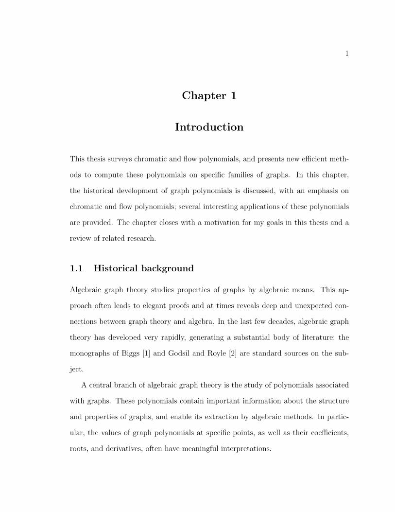
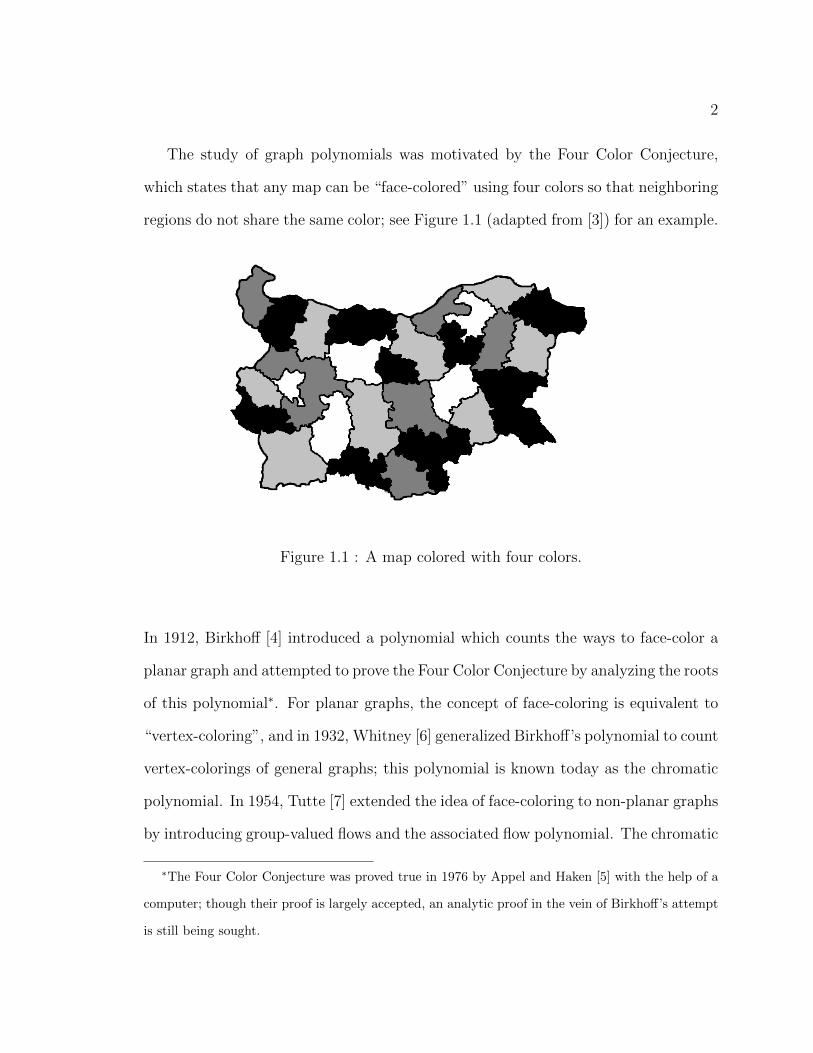
The study of graph polynomials was motivated by the Four Color Conjecture,
which states that any map can be “face-colored” using four colors so that neighboring
regions do not share the same color; see Figure 1.1 (adapted from [3]) for an example.
Figure 1.1 : A map colored with four colors.
In 1912, Birkhoff [4] introduced a polynomial which counts the ways to face-color a
planar graph and attempted to prove the Four Color Conjecture by analyzing the roots
of this polynomial∗. For planar graphs, the concept of face-coloring is equivalent to
“vertex-coloring”, and in 1932, Whitney [6] generalized Birkhoff’s polynomial to count
vertex-colorings of general graphs; this polynomial is known today as the chromatic
polynomial. In 1954, Tutte [7] extended the idea of face-coloring to non-planar graphs
by introducing group-valued flows and the associated flow polynomial. The chromatic
∗The Four Color Conjecture was proved true in 1976 by Appel and Haken [5] with the help of a
computer; though their proof is largely accepted, an analytic proof in the vein of Birkhoff’s attempt
is still being sought.
3
and flow polynomials are closely related, and are essentially equivalent in planar
graphs by graph duality; see Section 3.3 for more details.
Tutte and Whitney further generalized the chromatic and flow polynomials into
the two-variable Tutte polynomial [8], which includes as special cases several other
graph polynomials such as the reliability and Jones polynomials. Since then, graph
polynomials which are not direct specializations of the Tutte polynomial have also
been introduced; for instance, Hoede and Li [9] introduced the clique and indepen-
dence polynomials and McClosky, Simms, and Hicks [10] generalized the independence
polynomial into the co-k-plex polynomial. Studying these polynomials has been an
active area of research: Chia’s bibliography published in 1997 [11] counts 472 titles
on chromatic polynomials alone.
1.2 Importance and applications
The interest in graph polynomials is in the information they contain about the prop-
erties of graphs and networks, which can be easily obtained by algebraic techniques
but is much harder to access through purely graph theoretic approaches. Graph poly-
nomials also have connections to sciences such as statistical physics, knot theory, and
theoretical computer science. The chromatic and flow polynomials remain two of the
most well-studied single-variable graph polynomials, and are the focus of this thesis;
several important results about them are discussed in this section and in Chapter 3.
Naturally, the chromatic polynomial is often used in graph coloring problems,
which are widely applicable in scheduling, resource allocation, and pattern matching.
Read [12] gives two specific applications of the chromatic polynomial to the construc-
tion of timetables and the allocation of channels to television stations; see Kubale’s
monograph [13] for more graph coloring problems.
4
The chromatic polynomial is also used in statistical physics to model the be-
havior of ferromagnets and crystals; in particular, it is the zero-temperature limit
of the anti-ferromagnetic Potts model. The limit points of the roots of chromatic
polynomials indicate where physical phase transitions may occur [14]. Sokal [15] sur-
veys the applications of the multivariate Tutte polynomial — and its single-variable
specializations like the chromatic and flow polynomials — to statistical mechanics,
solid-state physics, and electrical circuit theory. In addition, his survey brings out
many connections and relations between graph polynomials, matroids, and practical
models.
Thomassen [16] showed that there exists a universal constant h ≈ 1.29 such that no
Hamiltonian graph has a root of its chromatic polynomial smaller than h. Hamilton
paths are essential to the Traveling Salesman Problem (TSP) which is very common
in practice but difficult to solve. Thus, if the chromatic polynomial of a graph can
be found efficiently, its roots can be approximated to an appropriate precision to
determine whether any of them are smaller than the constant h and possibly conclude
that the TSP has no solution on this graph.
Finally, the chromatic polynomial is related to the Stirling numbers [17, 18], the
Beraha numbers [19], and the golden ratio [20], and thus finds applications in a variety
of analytic and combinatorics problems.
There are important theoretical results and questions surrounding the flow poly-
nomial as well, such as the 6-flow theorem and the 5-flow conjecture. In addition,
the flow polynomial can be used to determine whether a graph has certain edge-
connectivity; this feature of the flow polynomial is discussed in more detail in Chap-
ter 3, along with other flow existence theorems and conjectures.
The flow polynomial also has an application in crystallography and statistical

5
mechanics as it is related to models of ice and crystal lattices (see [21]). In ice,
each oxygen atom is connected by hydrogen bonds to four other oxygen atoms; each
hydrogen bond contains a hydrogen atom which is closer to one of the two oxygen
atoms it connects [22]. This structure can be represented by a directed graph, where
the oxygen atoms are the vertices and the hydrogen bonds are directed edges pointing
to the closer oxygen atom. The flow polynomial of such a graph can be used to
count the number of permissible atomic configurations which conform to physical
restrictions. In turn, this can be used to model the physical properties of ice and
several other crystals, including potassium dihydrogen phosphate [23].
Results about the flow polynomial can also be used in estimating the error rate
of a computer program. The different decision paths taken by the program over all
possible executions can be represented by a control flow graph (cf. [24]); the degree
of the flow polynomial of such a graph is a measure of the corresponding program’s
complexity [25].
The chromatic and flow polynomials are also useful in computing or estimating
certain graph invariants, such as the chromatic, flow, independence, and clique num-
bers (indeed the chromatic and flow numbers of a graph with n vertices can be found
by evaluating the chromatic and flow polynomials at log n and 5 points, respectively).
These invariants are of great interest in extremal graph theory and are also impor-
tant characteristics of large networks [26, 27, 28]. For more applications of chromatic
and flow polynomials, see the comprehensive survey of Ellis-Monaghan and Merino
[29] and the bibliography therein. Further details on these two polynomials (some of
which more technical) are provided in Chapter 3.
6
1.3 Goals
Unfortunately, computing the chromatic and flow polynomials of a graph are very
challenging tasks. These problems are #P-hard for general graphs, and even for
bipartite planar graphs as shown in [30], and sparse graphs with |E| = O(|V |). In
fact, most of the coefficients of the chromatic and flow polynomials of general graphs
cannot even be approximated (see [31, 30]).
Thus, a large volume of work in this area is focused on exploiting the structure of
specific types of graphs in order to derive closed formulas, algorithms, or heuristics
for computing their chromatic and flow polynomials. In particular, classes of graphs
which are generalizations of trees, cliques, and cycles are frequently investigated.
For example, Wakelin and Woodall [32] consider a class of graphs called poly-
gon trees and find their chromatic polynomials; they also characterize the chromatic
polynomials of biconnected outerplanar graphs. Wakelin and Woodall also show that
a result from graph colorability is connected to graph reconstructibility, and it may
be worth exploring further connections between these two fields in future work. Fur-
thermore, Whitehead [33, 34] characterizes the chromatic polynomials of a class of
clique-like graphs called q-trees, Lazuka [35] obtains explicit formulas for the chro-
matic polynomials of cactus graphs, Gordon [36] studies Tutte polynomials of rooted
trees, and Mphako-Banda [37, 38] derives formulas for the chromatic, flow, and Tutte
polynomials of flower graphs.
In this thesis, I consider yet another generalization of trees, cliques, and cycles.
I define a generalized vertex join of a graph G to be the graph obtained by joining
an arbitrary multiset of the vertices of G to a new vertex. I compute the chromatic
polynomials of generalized vertex joins of trees, cliques, and cycles, and use the duality
of chromatic and flow polynomials to compute the flow polynomials of outerplanar
7
graphs and generalized wheel graphs. My results complement and expand the work of
Wakelin et al. [32] on chromatic polynomials of outerplanar graphs by characterizing
the flow polynomials of outerplanar graphs and the chromatic polynomials of their
duals, as well as finding the chromatic and flow polynomials of several other families of
graphs. Outerplanar graphs are a well-known and frequently used family of graphs,
and having access to their chromatic and flow polynomials is helpful for quickly
extracting certain information about them. In addition, my results can also be applied
to the Traveling Salesman Problem and to the anti-ferromagnetic Potts model in
the capacity of the applications mentioned earlier — either directly on the graphs I
consider, or on larger graphs which contain them as subgraphs.
8
Chapter 2
Preliminaries
This chapter recalls select graph theoretic notions and operations; some additional
definitions will be included in later chapters when needed. The background material
presented here is meant to be a quick reference rather than a self-contained founda-
tion; the reader is referred to [39] for a detailed introduction to graph theory. At
the end of this chapter, I introduce a new graph operation called a generalized vertex
join which will be used to characterize the families of graphs studied in the following
chapters.
2.1 Types of graphs
Different contexts call for different types of graphs. In the study of graph polynomials,
it is often useful to consider graphs with loops and multiple edges, and — when
studying flow — graphs with directed edges.
Definition 2.1 A simple undirected graph G = (V,E) consists of a vertex set V and
an edge set E of distinct two-element subsets of V .
Definition 2.2 An undirected multigraph G = (V,E) consists of a vertex set V and
an edge multiset E of not necessarily distinct one- or two-element subsets of V . A
loop in a multigraph is an edge which is a one-element subset of V and a multiple
edge is an edge which appears more than once in E.
9
Definition 2.3 A directed multigraph G = (V,E) consists of a vertex set V and an
edge multiset E of not necessarily distinct ordered pairs of elements of V . Given a
directed edge e = (u, v), u is the tail of e — denoted t(e) — and v is the head of e
— denoted h(e).
An implicit requirement in the preceding definitions is that V ∩E = ∅; in other words,
an object cannot be both a vertex and an edge. Unless otherwise stated, the second
of the three definitions will be intended in the sequel by the term ‘graph’. In addition,
for notational simplicity, e = uv will stand for an undirected edge e = {u, v} or a
directed edge e = (u, v) when there is no scope for confusion.
The number of times an edge e appears in E is the multiplicity of e. The underlying
set of E is the set E ′ which contains the (unique) elements of E. For example, if
E = {e1, e1, e2, e3, e3, e3}, then E ′ = {e1, e2, e3}. The underlying simple graph of
G = (V,E) is the graph (V,E ′ − {e : e is a loop}).
2.2 Planar graphs
Many of the graphs considered in the following chapters are planar graphs, which
means they can be drawn in the plane so that none of their edges cross. A graph
drawn in such a way is called a plane graph.
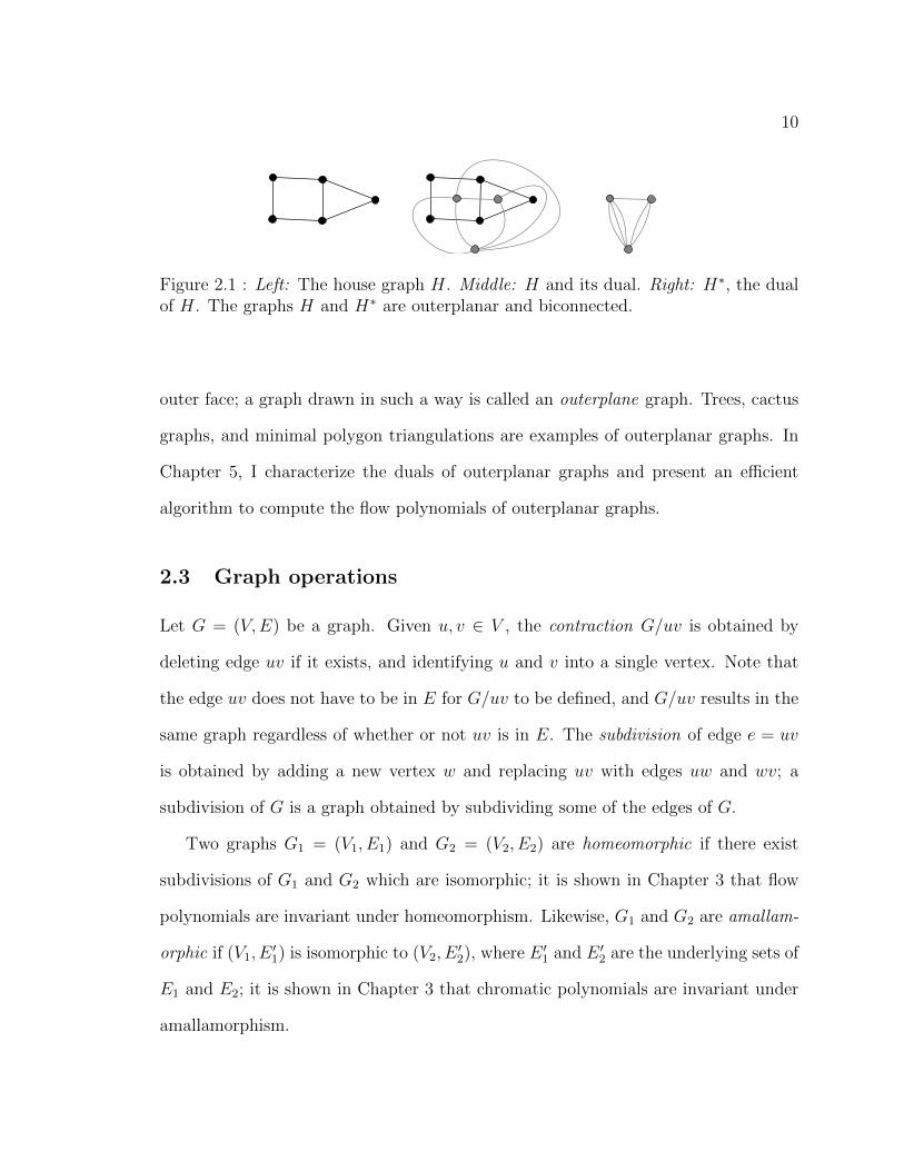
If G is a plane graph, its dual G∗ is a graph that has a vertex corresponding to
each face of G, and an edge joining the vertices corresponding to faces of G which
share an edge. Note that if G is connected, G = (G∗)∗. The weak dual of G is the
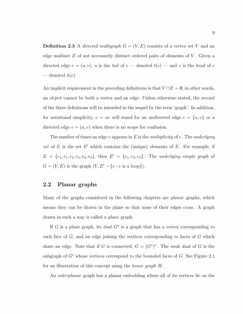
subgraph of G∗ whose vertices correspond to the bounded faces of G. See Figure 2.1
for an illustration of this concept using the house graph H.
An outerplanar graph has a planar embedding where all of its vertices lie on the
10
Figure 2.1 : Left: The house graph H. Middle: H and its dual. Right: H∗, the dualof H. The graphs H and H∗ are outerplanar and biconnected.
outer face; a graph drawn in such a way is called an outerplane graph. Trees, cactus
graphs, and minimal polygon triangulations are examples of outerplanar graphs. In
Chapter 5, I characterize the duals of outerplanar graphs and present an efficient
algorithm to compute the flow polynomials of outerplanar graphs.
2.3 Graph operations
Let G = (V,E) be a graph. Given u, v ∈ V , the contraction G/uv is obtained by
deleting edge uv if it exists, and identifying u and v into a single vertex. Note that
the edge uv does not have to be in E for G/uv to be defined, and G/uv results in the
same graph regardless of whether or not uv is in E. The subdivision of edge e = uv
is obtained by adding a new vertex w and replacing uv with edges uw and wv; a
subdivision of G is a graph obtained by subdividing some of the edges of G.
Two graphs G1 = (V1, E1) and G2 = (V2, E2) are homeomorphic if there exist
subdivisions of G1 and G2 which are isomorphic; it is shown in Chapter 3 that flow
polynomials are invariant under homeomorphism. Likewise, G1 and G2 are amallam-
orphic if (V1, E′1) is isomorphic to (V2, E
′2), where E ′1 and E ′2 are the underlying sets of
E1 and E2; it is shown in Chapter 3 that chromatic polynomials are invariant under
amallamorphism.
11
Given S ⊂ V , the induced subgraph G[S] is the subgraph of G whose vertex set is
S and whose edge set consists of all edges of G which have both ends in S. S ⊂ V is
an independent set if G[S] has no edges. Given S ⊂ E, the spanning subgraph G : S
is the subgraph of G whose vertex set is V and whose edge set is S.
An articulation point (also called a cut vertex ) is a vertex which, when removed,
increases the number of connected components in G. Similarly, a bridge (also called
a cut edge) is an edge which, when removed, increases the number of connected
components in G. G is biconnected if it has no articulation points, and a biconnected
component of G is a maximal subgraph of G which has no articulation points. The
graphs H and H∗ shown in Figure 2.1 are biconnected graphs.
An orientation ofG is an assignment of directions to the edges ofG; more precisely,
for each edge e = uv ∈ E, one of u and v is assigned to be h(e) and the other is
assigned to be t(e). An orientation of G is acyclic if it creates no directed cycles and
it is totally cyclic if it makes every edge belong to a directed cycle. We will see in
Chapter 3 that chromatic and flow polynomials can be used to count the number of
acyclic and totally cyclic orientations of a graph.
2.4 Generalized vertex join
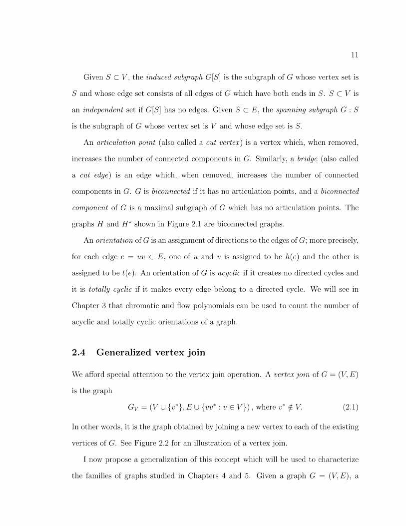
We afford special attention to the vertex join operation. A vertex join of G = (V,E)
is the graph
GV = (V ∪ {v∗}, E ∪ {vv∗ : v ∈ V }) , where v∗ /∈ V. (2.1)
In other words, it is the graph obtained by joining a new vertex to each of the existing
vertices of G. See Figure 2.2 for an illustration of a vertex join.
I now propose a generalization of this concept which will be used to characterize
the families of graphs studied in Chapters 4 and 5. Given a graph G = (V,E), a
12
v1
v2v5
v4 v3 v1
v2v5
v4 v3
v*
Figure 2.2 : Left: A graph H. Right: HV , the vertex join of H.
multiset S over V is a collection of vertices of V , each of which may appear more
than once in S.
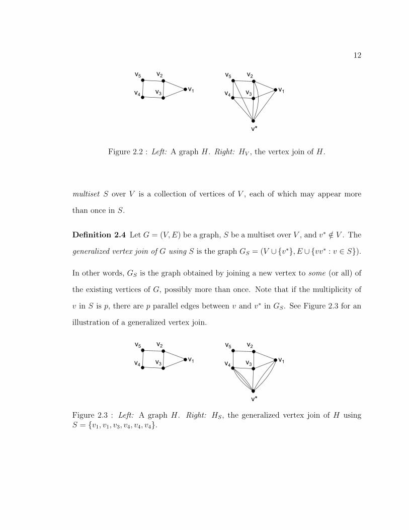
Definition 2.4 Let G = (V,E) be a graph, S be a multiset over V , and v∗ /∈ V . The
generalized vertex join of G using S is the graph GS = (V ∪ {v∗}, E ∪ {vv∗ : v ∈ S}).
In other words, GS is the graph obtained by joining a new vertex to some (or all) of
the existing vertices of G, possibly more than once. Note that if the multiplicity of
v in S is p, there are p parallel edges between v and v∗ in GS. See Figure 2.3 for an
illustration of a generalized vertex join.
v1
v2v5
v4 v3 v1
v2v5
v4 v3
v*
Figure 2.3 : Left: A graph H. Right: HS, the generalized vertex join of H usingS = {v1, v1, v3, v4, v4, v4}.
13
Chapter 3
Overview of chromatic and flow polynomials
This chapter surveys chromatic and flow polynomials and reveals their algebraic and
combinatorial properties. Dong [40] and Zhang [41] are standard resources on chro-
matic and flow polynomials respectively, while Tutte [42] relates the two polynomials
in a broader framework. These monographs provide a number of technical tools for
the computation of chromatic and flow polynomials, some of which are included in
this chapter. I apply these tools in the next two chapters to compute the chromatic
polynomials of generalized vertex joins of trees, cycles, and cliques, and the flow
polynomials of outerplanar graphs and “generalized wheel” graphs.
3.1 The chromatic polynomial
This section defines the chromatic polynomial and lists some of its algebraic and
combinatorial properties — in particular, information contained by its coefficients,
roots, derivatives, and evaluations at specific points. In addition, closed formulas are
given for the chromatic polynomials of some simple families of graphs, which will be
used in the following chapters.
3.1.1 Motivation
A vertex coloring of G is an assignment of colors to the vertices of G so that no edge
is incident to vertices of the same color. Many problems which involve vertex coloring
14
(which shall be referred to simply as coloring) are concerned with the following two
questions:
Q1. Can G be colored with t colors?
Q2. In how many ways can G be colored with t colors?
Clearly, the answer to Q2 contains the answer to Q1 and therefore Q2 is more general
and typically more difficult to answer. In a sense, Q1 is equivalent to asking “What
is the least number of colors needed to color G?” because if G can be colored with t
colors, it can be colored with t + 1 colors as well. Thus, if t∗ is the least number of
colors needed to color G, then Q1 can be answered in the affirmative for all t ≥ t∗
and in the negative for all t < t∗. The parameter t∗ (usually written χ(G)) which
answers Q1 is called the chromatic number of G. The rest of this section will analyze
the chromatic polynomial of G, which counts the number of ways to color G with t
colors and answers Q2.
3.1.2 Definition
Let G = (V,E) be a graph with n vertices. Formally, a t-coloring of G is a function
f : V → {1, . . . , t} such that f(u) 6= f(v) for any e = uv ∈ E. Let p(G; t) denote
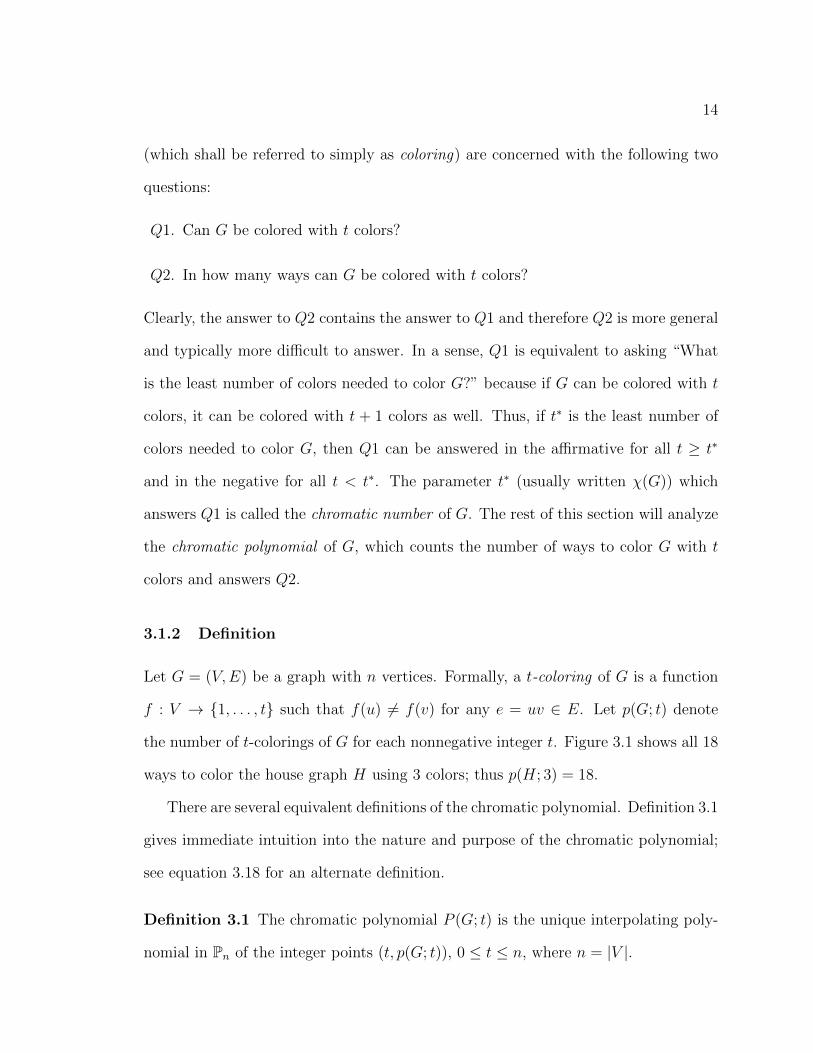
the number of t-colorings of G for each nonnegative integer t. Figure 3.1 shows all 18
ways to color the house graph H using 3 colors; thus p(H; 3) = 18.
There are several equivalent definitions of the chromatic polynomial. Definition 3.1
gives immediate intuition into the nature and purpose of the chromatic polynomial;
see equation 3.18 for an alternate definition.
Definition 3.1 The chromatic polynomial P (G; t) is the unique interpolating poly-
nomial in Pn of the integer points (t, p(G; t)), 0 ≤ t ≤ n, where n = |V |.
15
Figure 3.1 : All 3-colorings of the house graph H; p(H; 3) = 18.
Let us examine this definition closely. First, we can rightly claim that P (G; t) is the
unique interpolating polynomial of these n+1 points due to the following well-known
theorem (see [43] for a proof).
Theorem 3.1 (Unisolvence Theorem)
Let (x0, y0), . . . , (xn, yn) be points in R2 such that x0 < . . . < xn. There exists a
unique polynomial P ∈ Pn such that P (xi) = yi, 0 ≤ i ≤ n. �
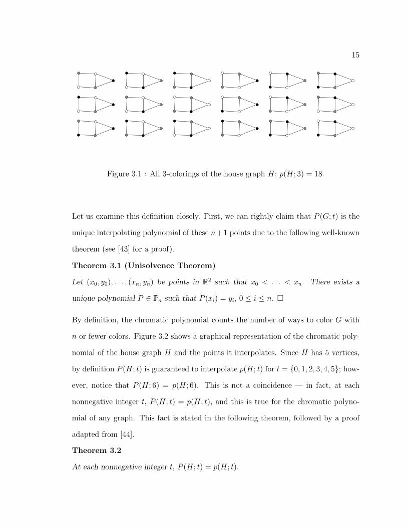
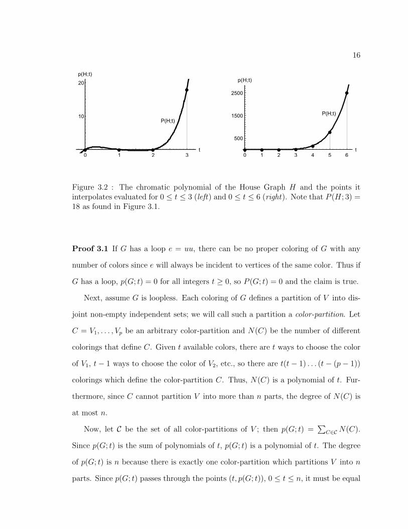
By definition, the chromatic polynomial counts the number of ways to color G with
n or fewer colors. Figure 3.2 shows a graphical representation of the chromatic poly-
nomial of the house graph H and the points it interpolates. Since H has 5 vertices,
by definition P (H; t) is guaranteed to interpolate p(H; t) for t = {0, 1, 2, 3, 4, 5}; how-
ever, notice that P (H; 6) = p(H; 6). This is not a coincidence — in fact, at each
nonnegative integer t, P (H; t) = p(H; t), and this is true for the chromatic polyno-
mial of any graph. This fact is stated in the following theorem, followed by a proof
adapted from [44].
Theorem 3.2
At each nonnegative integer t, P (H; t) = p(H; t).
16
P(H;t)
HH
P(H;t)
Figure 3.2 : The chromatic polynomial of the House Graph H and the points itinterpolates evaluated for 0 ≤ t ≤ 3 (left) and 0 ≤ t ≤ 6 (right). Note that P (H; 3) =18 as found in Figure 3.1.
Proof 3.1 If G has a loop e = uu, there can be no proper coloring of G with any
number of colors since e will always be incident to vertices of the same color. Thus if
G has a loop, p(G; t) = 0 for all integers t ≥ 0, so P (G; t) = 0 and the claim is true.
Next, assume G is loopless. Each coloring of G defines a partition of V into dis-
joint non-empty independent sets; we will call such a partition a color-partition. Let
C = V1, . . . , Vp be an arbitrary color-partition and N(C) be the number of different
colorings that define C. Given t available colors, there are t ways to choose the color
of V1, t− 1 ways to choose the color of V2, etc., so there are t(t− 1) . . . (t− (p− 1))
colorings which define the color-partition C. Thus, N(C) is a polynomial of t. Fur-
thermore, since C cannot partition V into more than n parts, the degree of N(C) is
at most n.
Now, let C be the set of all color-partitions of V ; then p(G; t) =∑
C∈C N(C).
Since p(G; t) is the sum of polynomials of t, p(G; t) is a polynomial of t. The degree
of p(G; t) is n because there is exactly one color-partition which partitions V into n
parts. Since p(G; t) passes through the points (t, p(G; t)), 0 ≤ t ≤ n, it must be equal

17
to P (G; t). �
The dependence of the chromatic polynomial on t is often implied in the context;
if there is no scope for confusion, P (G; t) can be abbreviated to P (G). By convention,
the graph with no vertices has chromatic polynomial equal to 1; this graph will be
excluded from further considerations.
3.1.3 Properties
Trivially, G can be colored by assigning a different color to each vertex; thus, χ(G) ≤
n. Unless t = χ(G), it is possible to have unused colors in a t-coloring; if t > n,
this becomes necessary. If t2 > t1 ≥ χ(G), any t2-coloring is also a t1-coloring and
p(G; t2) > p(G; t1). Thus, the sequence {p(G; t)}∞t=0 starts with χ(G) zeroes and then
strictly increases. The behavior of the chromatic polynomial of a general graph is
pictured in Figure 3.3.
0 n(G)
P(G;t)
Figure 3.3 : General appearance of the chromatic polynomial in the first quadrant
The coefficients, derivatives, roots, and evaluations of the chromatic polynomial
at certain points contain various information about the graph and are widely studied.
Below are several characteristics of the chromatic polynomial evaluated at specific
18
points.
• P (G; t) is the number of t-colorings of G for any nonnegative integer t.
• The chromatic number of G is the smallest positive integer t for which P (G; t) >
0. It can be determined from the chromatic polynomial by evaluating it at
t = 0, . . . , n (or faster, by a form of binary search).
• For any integers t2 > t1 ≥ χ(G), P (G; t2) > P (G; t1).
• Stanley [45] gives a combinatorial interpretation of the chromatic polynomial
evaluated at negative integers in terms of orientations of G. In particular,
|P (G;−1)| is the number of acyclic orientations of G.
Let P (G; t) = cntn + cn−1t
n−1 + . . . + c1t + c0. The coefficients of the chromatic
polynomial have the following properties:
• c0, . . . , cn are integers.
• cn = 1.
• cn−1 = −m where m is the number of edges of G.
• If m 6= 0,∑n
i=1 ci = 0; if m = 0, P (G; t) = tn and∑n
i=1 ci = 1.
• c0, . . . , ck−1 = 0 and ck, . . . , cn 6= 0 where k is the number of components of G.
• ci ≥ 0 if i = n mod 2, ci ≤ 0 if i 6= n mod 2, i.e., the coefficients alternate signs.
• c1, . . . , cn−1 are #P-hard to compute, even for bipartite and planar graphs [30].
◦ Unimodal conjecture [12]: the sequence {|ci|}ni=1 is unimodal, i.e., for some
ci, |c1| ≤ . . . ≤ |ci| ≥ . . . ≥ |cn|. This conjecture has been proven true for
outerplanar graphs [46] and some other families of graphs.
19
The derivative of the chromatic polynomial has interesting properties as well, in
particular when evaluated at 1. The quantity θ(G) = (−1)n ddtP (G; t)
∣∣t=1
is called the
chromatic invariant of G and has been widely studied. Below are two results due to
Crapo [47] and Brylawski [48], respectively; in addition, see [49, 50] for combinatorial
interpretations of θ(G).
• θ(G) 6= 0 if and only if G is biconnected.
• θ(G) = 1 if and only if G is series-parallel. Series-parallel (SP) graphs are used
to model electrical circuits. It is useful to know that a graph is SP because
many NP-hard problems can be solved in linear time over SP graphs (cf. [51]).
Finally, the roots of P (G; t) — called the chromatic roots of G — contain significant
information about the structure of G. The set of chromatic roots of all graphs (or
of special families of graphs) is interesting in its own right; recall that Birkhoff’s
motivation for introducing the chromatic polynomial was to investigate gaps in the
set of chromatic roots of planar graphs in order to prove the Four Color Theorem.
• The number of biconnected components of G is the multiplicity of the root ‘1’
of P (G; t) [52].
• If P (G; t) has a noninteger root less than or equal to h ≈ 1.29559, then G has
no Hamiltonian path [16].
• Let R be the set of all chromatic roots (of all graphs). R is dense in [32/27,∞)
[53] and dense in C [54]. Moreover, R∩ (−∞, 32/27) = {0, 1}, i.e., there are no
real chromatic roots less than 32/27 other than 0 and 1 [55].
• Not every complex number and real number in [32/27,∞) is a chromatic root;
for example, φ+ 1 =√5+32
is not a root of any chromatic polynomial [56].

20
• 5-Color Theorem [57]: Planar graphs have no real chromatic roots in [5,∞).
• 4-Color Theorem [5]: 4 is not a chromatic root of planar graphs. Appel and
Haken proved this by eliminating a long list of minimum counterexamples us-
ing a computer; it is still an open problem to prove the 4-Color Theorem by
analyzing chromatic roots.
◦ Birkhoff-Lewis Conjecture [58]: Planar graphs have no real roots in [4,∞).
3.1.4 Computation
Computing the chromatic polynomial of a graph from its definition is highly impracti-
cal. Fortunately, there are several well-known formulas which aid in this computation
by reducing the chromatic polynomial of a graph into that of smaller graphs. The
most notable of these is the deletion-contraction formula, which is discussed next.
Let G = (V,E) be a graph and u and v be two vertices of G. The t-colorings
of G can be split up into those in which u and v have different colors and those in
which they have the same color. Adding the edge uv to G assures that u and v have
different colors, and identifying u and v into a single vertex assures that they have
the same color. Thus, for every coloring of G in which u and v have different colors,
there is exactly one coloring of G + uv and for every coloring of G in which u and v
have the same color, there is exactly one coloring of G/uv. This observation yields
the addition-contraction formula:
P (G) = P (G+ e) + P (G/e) for any e = uv, where u, v ∈ V. (3.1)
Alternately, we can set H = G− e for some edge e of G; then, P (G− e) = P (H) =
P (H + e) + P (H/e) = P (G) + P ((G − e)/e), but (G − e)/e = G/e, so P (G) =
21
P (G− e)− P (G/e). This yields the deletion-contraction formula:
P (G) = P (G− e)− P (G/e) for any e = uv, where u, v ∈ V. (3.2)
Equations 3.1 and 3.2 can be used to recursively compute the chromatic polyno-
mial of any graph G. In particular, each application of 3.2 reduces G into two graphs
each with one fewer edge and, after enough iterations, into graphs with no edges;
thus, P (G) can be expressed as a linear combination of the chromatic polynomials of
empty graphs. Similarly, 3.1 can be used to express P (G) as a linear combination of
the chromatic polynomials of complete graphs. The chromatic polynomials of empty
graphs and complete graphs can be computed directly using combinatorial arguments
as shown in Examples 3.1 and 3.2 in the next section.
The computer algebra system Mathematica has a built-in ChromaticPolynomial
function which uses the addition-contraction formula to compute the chromatic poly-
nomials of dense graphs, and the deletion-contraction formula for sparse graphs [59].
Version 10 of Mathematica has a more efficient implementation of the deletion-
contraction algorithm as the ChromaticPolynomial function from the Combinatorica
package is built into the Wolfram System. However, this implementation no longer
uses the addition-contraction formula which causes it to perform poorly on dense
graphs, as revealed by the computational results included in Chapter 6.
It can be shown (cf. [60]) that an algorithm based on the recurrences (3.1) and
(3.2) has a worst-case run time of O(φn+m), where φ = 1+√5
2is the golden ratio and
m is the number of edges of G. Some improvements on this algorithm have been
made by Bjorklund [61]. With a priori information about the structure of the graph,
the run time of this algorithm can be improved significantly; in particular, the order
of the edges being contracted and deleted can be chosen strategically to obtain large
22
subgraphs (such as cliques) whose chromatic polynomials are known. Moreover, there
are polynomial time algorithms for computing the chromatic polynomials of graphs
with bounded clique-width and tree-width. In particular, Makowsky et al. [62] show
that P (G) can be computed in O(nf(w)) time, where w is the clique-width of G and
f(w) ≤ 3 ·2w+2. However, even for w = 2, this yields a worst-case run time of O(n48).
Similarly, Andrzejak’s algorithm [63] for computing the Tutte polynomials of graphs
of tree-width w has a worse-case run time of O(n109.6) when w = 2. Thus, these
algorithms are principally of theoretical value.
There are several other reduction formulas for chromatic polynomials which are
outlined next; see Tutte [42] for detailed proofs. If G has two subgraphs whose
intersection is a clique, then the chromatic polynomials of those subgraphs can be
combined to compute the chromatic polynomial of G in the following way:
If G = G1 ∪G2 and G1 ∩G2 = Kr, then P (G) =P (G1)P (G2)
P (Kr). (3.3)
Note that articulation points are cliques of size 1, so this formula can be used to
separate a graph into biconnected components to find its chromatic polynomial. Fur-
thermore, disjoint components of a graph can be colored independently; thus, to
compute the chromatic polynomial of a disconnected graph, it suffices to compute
the chromatic polynomials of each component separately:
If G = G1 ∪G2 and G1 ∩G2 = ∅, then P (G) = P (G1)P (G2). (3.4)
If G has a vertex v which is connected to every other vertex in G, then
P (G; t) = tP (G− v; t− 1). (3.5)
23
Equivalently, this formula can be used to compute the chromatic polynomial of a
vertex join GV of G as shown below:
P (GV ; t) = tP (G; t− 1). (3.6)
However, (3.6) is not applicable to a generalized vertex join since it requires every
vertex in G to be connected to the added vertex v∗. Finally, multiple edges between
vertices u and v have no more effect on the coloring of G than a single edge between
u and v; thus,
If e ∈ E is a multiple edge, then P (G) = P (G− e). (3.7)
This implies that the chromatic polynomial of a multigraph is equal to the chro-
matic polynomial of its underlying simple graph and that the chromatic polynomial
is invariant under amallamorphism. However, it is still sometimes useful to consider
the chromatic polynomials of graphs with multiple edges (such as graphs obtained
through a generalized vertex join) because the duals of these graphs form a more
general family. This matter will be discussed in Section 3.3.
3.1.5 Special cases
Using the decomposition techniques outlined thus far along with simple combinatorial
arguments, closed formulas for the chromatic polynomials of some specific graphs can
be derived. Some of these closed formulas will be used in Chapter 4 to compute the
chromatic polynomials of more complex graphs. For more detailed proofs and other
examples, see [40].
Example 3.1 Let G be the empty graph on n vertices. Given t available colors, each
24
vertex in G can be colored independently in t ways. Thus,
P (G; t) = tn. (3.8)
Example 3.2 Let Kn be the complete graph on n vertices. Since all vertices in Kn
are mutually adjacent, after fixing the color of one arbitrary vertex, each successive
vertex can be colored in one fewer ways. With t available colors, the first vertex can
be colored in t ways, the second in t− 1 ways, etc., so
P (Kn; t) = t(t− 1) . . . (t− (n− 1)) =n−1∏i=0
(t− i). (3.9)
Example 3.3 Let G be an arbitrary tree on n vertices. A tree on one vertex can be
colored in t ways, and adding a leaf vertex to a tree increases the number of colorings
by a factor of t−1, since the added vertex cannot have the same color as its neighbor.
Thus,
P (G; t) = t(t− 1)n−1. (3.10)
Example 3.4 Let Cn be the cycle on n vertices. Applying the deletion-contraction
formula to an arbitrary edge yields a tree and a cycle on n − 1 vertices; using this
formula recursively yields
P (Cn; t) = (t− 1)n + (−1)n(t− 1). (3.11)
Example 3.5 Let Wn be the wheel with n spokes. A wheel is a vertex join of a cycle
on n vertices; applying equation 3.6 to equation 3.11 yields
P (Wn; t) = t((t− 2)n−1 + (−1)n−1(t− 2)
). (3.12)
25
3.2 The flow polynomial
This section introduces integer-valued and group-valued flows and defines the flow
polynomial. Several algebraic and combinatorial properties of the flow polynomial
are discussed, along with theorems and conjectures about the existence of flows in
certain conditions.
3.2.1 Motivation
A plane graph G has a well-defined dual whose vertices correspond to faces of G, so in
plane graphs, the concept of face-coloring is essentially equivalent to vertex-coloring.
However, face-coloring cannot be defined on general graphs in the same sense as on
planar graphs, since non-planar graphs do not have well-defined faces (in a planar
embedding). To this end, Tutte introduced the theory of group- and integer-valued
flows as a way to extend face-coloring from planar graphs to general graphs. A group-
valued (respectively, integer-valued) flow on an orientation of G is an assignment of
values to the edges of G from an Abelian group (respectively, from a set of integers)
so that flow is conserved at each vertex of G.
The theory of group- and integer-valued flows is connected to some of the deepest
and most challenging notions in graph theory such as the cycle-double cover conjecture
[64] and the Four Color Theorem. Many problems which involve flows are concerned
with whether a graph admits a certain flow, and if so — in how many different ways.
Just as the chromatic polynomial counts the number of graph colorings, there is a
flow polynomial which counts the number of group-valued flows on a given graph.
Defining and studying this polynomial will be the subject of the remainder of this
section.

26
3.2.2 Definition
To define group-valued flows, recall first the definition of an Abelian algebraic group.
Definition 3.2 An Abelian group (A,+) is an ordered pair consisting of a set A and
a binary operation ‘+’ which together satisfy the following conditions:
Closure: a, b ∈ A =⇒ a+ b ∈ A
Associativity: a, b, c ∈ A =⇒ a+ (b+ c) = (a+ b) + c
Identity element: ∃ 0 ∈ A such that 0 + a = a+ 0 = a ∀a ∈ A
Inverse elements: ∀a ∈ A ∃ (−a) ∈ A such that a+ (−a) = (−a) + a = 0
Commutativity: a, b ∈ A =⇒ a+ b = b+ a.
When there is no scope for confusion, the group (A,+) is abbreviated as A; the
cardinality of group (A,+) is equal to |A|, the number of elements in A. A finite
Abelian group is an Abelian group of finite cardinality. A simple example of a finite
Abelian group is the cyclic group (Zt,+) where Zt = {0, 1, . . . , t − 1} and ‘+’ is
addition modulo t. In fact, Zt is essentially the only finite Abelian group that will be
required in the context of this chapter. With this in mind, a group-valued flow can
be defined as follows.
Definition 3.3 Let A be a finite Abelian group and G = (V,E) be a graph with a
fixed orientation. An A-flow on this orientation of G is a function φ : E → A such
that for each v ∈ V ,∑
h(e)=v φ(e) =∑
t(e)=v φ(e). An A-flow φ is nowhere-zero if
φ(e) 6= 0 for all e ∈ E.
The condition∑
h(e)=v φ(e) =∑
t(e)=v φ(e) in Definition 3.3 is sometimes called
Kirchhoff’s Law (commonly applied as the principle of conservation of energy in
27
electrical circuits) and means that the total flow entering each vertex is equal to
the total flow leaving each vertex. Nowhere-zero A-flows are also called group-valued
flows and modular flows. Taking A = Z and |φ(e)| < t for each e ∈ E in the definition
above yields another type of flow called a nowhere-zero t-flow. This is stated more
formally as follows.
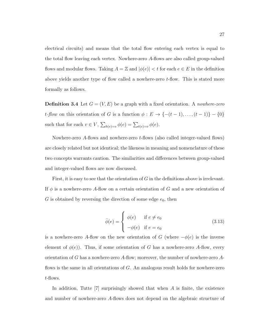
Definition 3.4 Let G = (V,E) be a graph with a fixed orientation. A nowhere-zero
t-flow on this orientation of G is a function φ : E → {−(t − 1), . . . , (t − 1)} − {0}
such that for each v ∈ V ,∑
h(e)=v φ(e) =∑
t(e)=v φ(e).
Nowhere-zero A-flows and nowhere-zero t-flows (also called integer-valued flows)
are closely related but not identical; the likeness in meaning and nomenclature of these
two concepts warrants caution. The similarities and differences between group-valued
and integer-valued flows are now discussed.
First, it is easy to see that the orientation of G in the definitions above is irrelevant.
If φ is a nowhere-zero A-flow on a certain orientation of G and a new orientation of
G is obtained by reversing the direction of some edge e0, then
φ(e) =
φ(e) if e 6= e0
−φ(e) if e = e0
(3.13)
is a nowhere-zero A-flow on the new orientation of G (where −φ(e) is the inverse
element of φ(e)). Thus, if some orientation of G has a nowhere-zero A-flow, every
orientation of G has a nowhere-zero A-flow; moreover, the number of nowhere-zero A-
flows is the same in all orientations of G. An analogous result holds for nowhere-zero
t-flows.
In addition, Tutte [7] surprisingly showed that when A is finite, the existence
and number of nowhere-zero A-flows does not depend on the algebraic structure of

28
A but only on its cardinality. Thus, without loss of generality, the group A in a
nowhere-zero A-flow with |A| = t can be taken to be Zt. Tutte also showed that G
has a nowhere-zero t-flow if and only if it has a nowhere-zero Zt-flow. However, the
number of nowhere-zero t-flows on G is not necessarily the same as the number of
nowhere-zero Zt-flows. Finally, a graph with a bridge b does not admit a nowhere-zero
t-flow or a nowhere-zero Zt-flow, since a non-zero flow on b would create a non-zero
total outflow from some component of G− b (see Lemma 3.1 for more details). These
results are summarized in the following theorem.
Theorem 3.3 (Tutte [7, 42])
Let G be a bridgeless graph with a fixed orientation and A be an Abelian group with
|A| = t. Then, the following statements are equivalent:
1. G has a nowhere-zero t-flow
2. G has a nowhere-zero Zt-flow
3. G has a nowhere zero A-flow
4. Every orientation of G has a nowhere-zero t-flow
5. Every orientation of G has a nowhere-zero Zt-flow
6. Every orientation of G has a nowhere-zero A-flow. �
Let G = (V,E) be a graph with n vertices, m edges, and k components and let
f(G; t) denote the number of nowhere-zero Zt-flows on G for each positive integer t.
Figure 3.4 shows the two nowhere-zero Z3-flows and the six nowhere-zero Z4-flows on
an orientation of the house graph H; thus f(H; 3) = 2 and f(H; 4) = 6.
The following lemma of Tutte [42] allows nowhere-zero Zt-flows to be counted
recursively; it will be useful in defining and computing the flow polynomial.

29
1
1
12
1
2
2
2
21
2
1
1
1
12
1
2
1
1
13
2
3
2
2
21
3
1
2
2
23
1
3
3
3
31
2
1
3
3
32
3
2
Figure 3.4 : Left: All nowhere-zero Z3-flows on an orientation of the house graph H;f(H; 3) = 2. Right: All nowhere-zero Z4-flows on H; f(H; 4) = 6.
Lemma 3.1
Let G be a graph and e be an edge of G. Then, for each positive integer t,
f(G; t) =
f(G/e; t)− f(G− e; t) if e is not a loop
(t− 1)f(G− e; t) if e is a loop
(t− 1) if G = C1
0 if G has a bridge
(3.14)
Proof 3.2 If e is a loop, then f(G; t) = (t− 1)f(G− e; t), since there are f(G− e; t)
nowhere-zero Zt-flows on G− e, and any of the t− 1 nonzero members of Zt can be
assigned to e to produce a nowhere-zero flow on G.
Next, suppose e is not a loop. Let f1 be the set of Zt-flows which are nowhere-zero
on G− e and in which e may have 0 flow. For every Zt-flow in f1, there is exactly one
nowhere-zero Zt-flow on G/e. Let f2 be the set of Zt-flows which are nowhere-zero
on G − e and in which e does have 0 flow. For every Zt-flow in f2, there is exactly
one nowhere-zero Zt-flow on G− e. The nowhere-zero Zt-flows on G can be obtained
by subtracting f2 from f1. Thus, f(G, t) = f(G/e, t) − f(G − e, t) for any non-loop
30
edge e.
Now consider the graph C1 consisting of one loop; f(C1; t) = t − 1 since each of
the t − 1 nonzero members of Zt can be assigned to the loop to produce a non-zero
flow.
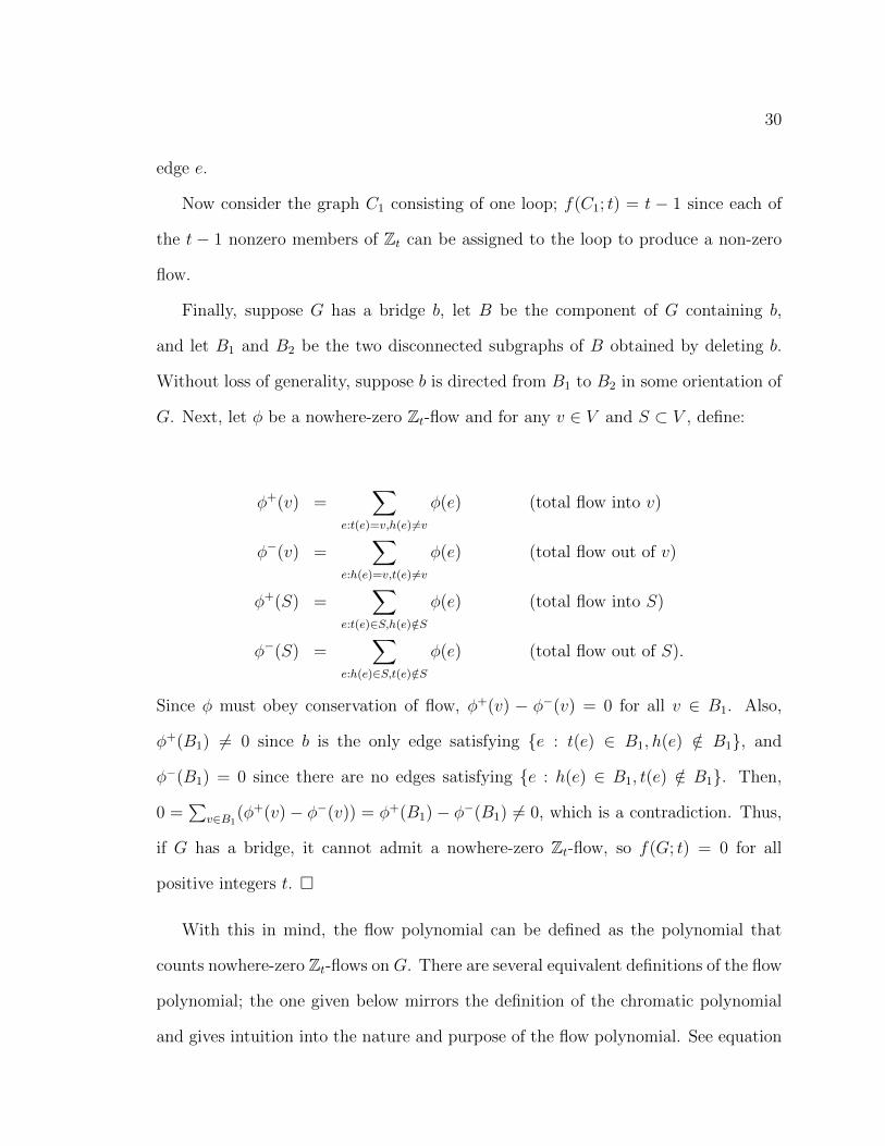
Finally, suppose G has a bridge b, let B be the component of G containing b,
and let B1 and B2 be the two disconnected subgraphs of B obtained by deleting b.
Without loss of generality, suppose b is directed from B1 to B2 in some orientation of
G. Next, let φ be a nowhere-zero Zt-flow and for any v ∈ V and S ⊂ V , define:
φ+(v) =∑
e:t(e)=v,h(e)6=v
φ(e) (total flow into v)
φ−(v) =∑
e:h(e)=v,t(e)6=v
φ(e) (total flow out of v)
φ+(S) =∑
e:t(e)∈S,h(e)/∈S
φ(e) (total flow into S)
φ−(S) =∑
e:h(e)∈S,t(e)/∈S
φ(e) (total flow out of S).
Since φ must obey conservation of flow, φ+(v) − φ−(v) = 0 for all v ∈ B1. Also,
φ+(B1) 6= 0 since b is the only edge satisfying {e : t(e) ∈ B1, h(e) /∈ B1}, and
φ−(B1) = 0 since there are no edges satisfying {e : h(e) ∈ B1, t(e) /∈ B1}. Then,
0 =∑
v∈B1(φ+(v)− φ−(v)) = φ+(B1)− φ−(B1) 6= 0, which is a contradiction. Thus,
if G has a bridge, it cannot admit a nowhere-zero Zt-flow, so f(G; t) = 0 for all
positive integers t. �
With this in mind, the flow polynomial can be defined as the polynomial that
counts nowhere-zero Zt-flows on G. There are several equivalent definitions of the flow
polynomial; the one given below mirrors the definition of the chromatic polynomial
and gives intuition into the nature and purpose of the flow polynomial. See equation
31
3.19 for an alternate definition.
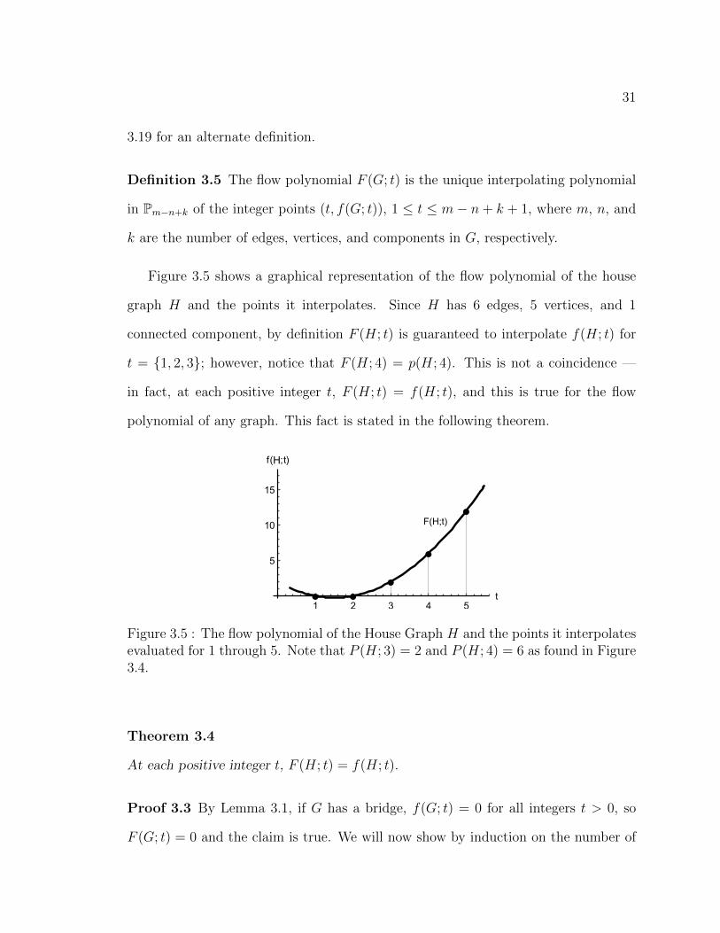
Definition 3.5 The flow polynomial F (G; t) is the unique interpolating polynomial
in Pm−n+k of the integer points (t, f(G; t)), 1 ≤ t ≤ m− n+ k + 1, where m, n, and
k are the number of edges, vertices, and components in G, respectively.
Figure 3.5 shows a graphical representation of the flow polynomial of the house
graph H and the points it interpolates. Since H has 6 edges, 5 vertices, and 1
connected component, by definition F (H; t) is guaranteed to interpolate f(H; t) for
t = {1, 2, 3}; however, notice that F (H; 4) = p(H; 4). This is not a coincidence —
in fact, at each positive integer t, F (H; t) = f(H; t), and this is true for the flow
polynomial of any graph. This fact is stated in the following theorem.
F(H;t)
H
Figure 3.5 : The flow polynomial of the House Graph H and the points it interpolatesevaluated for 1 through 5. Note that P (H; 3) = 2 and P (H; 4) = 6 as found in Figure3.4.
Theorem 3.4
At each positive integer t, F (H; t) = f(H; t).
Proof 3.3 By Lemma 3.1, if G has a bridge, f(G; t) = 0 for all integers t > 0, so
F (G; t) = 0 and the claim is true. We will now show by induction on the number of

32
edges that for any bridgeless graph G, there exists a degree m − n + k polynomial
F (G; t) such that F (G; t) = f(G; t) at each positive integer t. This polynomial must
be the flow polynomial, since two polynomials of degree m − n + k which agree at
m− n+ k + 1 points must be identical by Theorem 3.1.
If G is a bridgeless graph with one edge, that edge must be a loop, so f(G; t) = t−1
by Lemma 3.1. Moreover, m − n + k = 1 since n = k and m = 1, so the degree 1
polynomial F (G; t) = t− 1 satisfies the conditions of the theorem.
Now, suppose G is a bridgeless graph with m > 1 edges, n vertices, and k com-
ponents, and let e be an edge of G. If e is not a loop, it is easy to see that G/e
is bridgeless and has k components, n − 1 vertices and m − 1 edges. Thus, by in-
duction, there exists a polynomial F (G/e; t) of degree m − n + k equal to f(G/e; t)
for all positive integers t. Similarly, G − e has k components, n vertices, and m − 1
edges. If G − e is bridgeless, by induction there exists a polynomial F (G − e; t) of
degree m − n + k − 1 equal to f(G − e; t) for all positive integers t; if G − e has a
bridge, F (G − e; t) = 0. Thus, we define F (G; t) = F (G/e; t) − F (G − e; t), so that
F (G; t) = F (G/e; t)− F (G− e; t) = f(G/e; t)− f(G− e; t) = f(G; t), at all positive
integers t, and F (G; t) has degree m− n+ k.
If e is a loop, it is easy to see that G/e is bridgeless and has k components, n
vertices and m − 1 edges. Thus, by induction, there exists a polynomial F (G/e; t)
of degree m− n+ k − 1 equal to f(G/e; t) for all positive integers t. By Lemma 3.1
f(G; t) = (t − 1)f(G − e; t); thus, we define F (G; t) = (t − 1)F (G − e; t), so that
F (G; t) = (t − 1)F (G − e; t) = (t − 1)f(G − e; t) = f(G; t), and F (G; t) has degree
m− n+ k. This completes the induction. �
Remark 3.1 It should be noted that while the chromatic polynomial is often intro-
duced rigorously in textbooks and papers, such introductions to the flow polynomial
33
are somewhat rare in the literature. The proofs of Lemma 3.1 and Theorem 3.4 in-
cluded here are modeled after the discussions and proofs in [39, 41, 42] and attempt
to provide (perhaps for the first time) a unified and rigorous introduction to the flow
polynomial. �
Note that the number of nowhere-zero t-flows is generally not equal to F (G; t);
however, F (G; t) > 0 if and only if G admits a nowhere-zero t-flow. The dependence
of the flow polynomial on t is often implied in the context; if there is no scope
for confusion, F (G; t) can be abbreviated to F (G). By convention, the graph with
zero edges has flow polynomial equal to 1; this graph will be excluded from further
considerations in this section.
Just as the chromatic number χ(G) is the smallest number of colors needed to
color G, the flow number of G, written ψ(G), is the smallest positive t for which G has
a nowhere-zero t-flow (and therefore a nowhere-zero Zt-flow). While the chromatic
number of a graph can be arbitrarily high (for example, χ(Kn) = n), the same is not
true of the flow number – in fact, Seymour [65] showed that the flow number of any
graph is at most 6. Nevertheless, for any t, deciding whether G has a nowhere-zero
t-flow is an NP-hard problem. Indeed, even for planar graphs and t = 3, this problem
is NP-complete [66].
3.2.3 Properties
Knowing the flow polynomial of a graph allows the flow number to be determined
in linear time. In addition, the coefficients, roots, and evaluations of the flow poly-
nomial at certain points contain various information about the graph. Below are
several characteristics of the flow polynomial of a bridgeless graph G with n vertices,
evaluated at specific points.
34
• F (G; t) is the number of nowhere-zero Zt-flows on G for any positive integer t.
• In general, for a positive integer t, F (G; t) is not the number of nowhere-zero t-
flows on G; however, G admits a nowhere-zero t-flow if and only if F (G; t) > 0.
Recently, Kochol [67] showed that there is a polynomial FZ(G; t) 6= F (G; t)
which counts the number of nowhere-zero t-flows in G, and that F and FZ can
be used to estimate one another.
• 6-flow Theorem: F (G; 6) > 0, i.e., every bridgeless graph admits a nowhere-
zero 6-flow. This result is due to Seymour [65] and is an improvement over the
earlier result of Jaeger and Kilpatrick who showed that every bridgeless graph
has a nowhere-zero 8-flow [68, 69].
◦ 5-flow Conjecture [7] : F (G; 5) > 0, i,e., every bridgeless graph has a nowhere-
zero 5-flow. This conjecture cannot be strengthened to “F (G; 4) > 0”, since the
Petersen graph does not admit a nowhere-zero 4-flow.
• The flow number of G is the smallest positive integer t for which F (G; t) > 0.
In view of the 6-flow Theorem, ψ(G) can be determined by evaluating F (G; t)
at t = 1, . . . , 5.
• For any integers t2 ≥ t1 ≥ ψ(G), F (G; t2) ≥ F (G; t1).
• Stanley and Noy [45, 70] give a combinatorial interpretation of the flow polyno-
mial evaluated at negative integers in terms of orientations of G. In particular,
|F (G;−1)| is the number of totally cyclic orientations of G.
• F (G; 1) = 0, i.e., no graph admits a nowhere-zero 1-flow.
• F (G; 2) > 0 if and only if G is Eulerian.
35
• F (G; t) > 0 for all real t > 2 log2 n. This result is particularly useful for graphs
with few vertices but many double edges and loops [71].
Let F (G; t) = fνtν + . . . + f1t + f0. The coefficients of the flow polynomial have the
following properties:
• f0, . . . , fν are integers.
• fν = 1.
• Computing f0, . . . , fν is #P-hard, even for bipartite planar graphs [30].
• Dong and Koh [72] have showed that for 0 ≤ i ≤ ν, |fi| is bounded above by
the coefficient of ti in the expansion of a fixed polynomial of degree ν.
The degree ν of the flow polynomial has several interesting properties as well. Let G
be a graph with m edges, n vertices, and k components; then,
• The degree ν of F (G; t) is equal to m − n + k. This quantity is called the
cyclomatic number of G, written ν(G).
• The cyclomatic number is equal to dimension of the cycle space of G — the
set of all even subgraphs of G. There are many other connections between
integer flows and the cycle space of G, especially involving cycle covers; Zhang’s
monograph [41] is dedicated to this subject.
• A control flow graph is a directed graph representation of the different decision
paths that can be taken in all possible executions of a computer program (cf.
[24]). McCabe [25] introduced the cyclomatic complexity number of a program
as a measure of a program’s complexity; this number is the cyclomatic number
36
of the corresponding control flow graph. It is interpreted as the amount of
decision logic in a program and a high cyclomatic complexity number correlates
with a high error rate of the program.
Finally, the flow polynomial contains information about the edge-connectivity of the
graph. Below are some results about the existence of flows under given conditions.
Recall that a graph has a nowhere-zero t-flow if and only if it has a nowhere-zero
Zt-flow if and only if F (G; t) > 0; thus, the following results can also be stated in
terms of the flow polynomial; for example, the first item below can be interpreted as
“If F (G; 3) = 0, then G is not 6-edge-connected”.
• Every 6-edge-connected graph has a nowhere-zero 3-flow [73]. This was an
improvement over Thomassen’s result that every 8-edge-connected graph has a
nowhere-zero 3-flow [74]. Both of these important results are very recent, and
have encouraged further research in the field.
• 4-flow Theorem [75]: Every 4-edge-connected graph has a nowhere-zero 4-flow.
◦ 3-flow Conjecture [76]: Every 4-edge-connected graph has a nowhere-zero 3-flow.
• A 3-regular graph admits a nowhere-zero 3-flow if and only if it is bipartite [75].
3.2.4 Computation
Just as the chromatic polynomial can be computed for general graphs using the
deletion-contraction and addition-contraction formulas, so too can the flow polyno-
mial be computed using the equations in Lemma 3.1 recursively. The computational
analysis of such an algorithm is analogous to the one given in the previous section for
the chromatic polynomial.
37
Furthermore, if a graph G has k > 1 components, the following identity allows
the flow polynomial of each component to be found separately:
If G = G1 ∪G2 and G1 ∩G2 = ∅, then F (G) = F (G1)F (G2). (3.15)
In fact, since flow is measured over edges and not vertices, this claim can be strength-
ened to biconnected components:
If G = G1 ∪G2 and G1 ∩G2 = {v}, then F (G) = F (G1)F (G2). (3.16)
See [42] for proofs of these identities and [41, 77] for other decomposition formulas.
In addition, it will be shown in the next section that for planar graphs, many of the
identities developed for chromatic polynomials can also be used in the computation
of flow polynomials.
3.3 Connections between chromatic and flow polynomials
The chromatic and flow polynomials are closely connected, especially in planar graphs.
Intuitively, in planar graphs vertex coloring is equivalent to face-coloring, and face-
coloring is generalized by nowhere-zero flows. Thus, it can be expected that the
chromatic and flow polynomials are very similar in planar graphs. Indeed, the follow-
ing result by Jaeger [78] confirms this intuition:
If G is planar, then F (G) =1
tP (G∗). (3.17)
Thus, many of the identities developed for chromatic polynomials can also be used
in the computation of flow polynomials, as the flow polynomial can be easily obtained
from the chromatic polynomial in planar graphs.
38
The duality relation of chromatic and flow polynomials will be used in the next
two chapters to compute the flow polynomials of outerplanar graphs and generalized
wheel graphs from the chromatic polynomials of their duals. At this point, a short
discussion on the generalized vertex join operation is warranted.
Remark 3.2 Let G = (V,E) be any graph, S be a multiset over V , and S ′ be the
underlying set of S. Recall that a generalized vertex join of G is obtained by joining
each vertex in S to a new vertex v∗. By equation 3.7, P (GS) = P (GS′). Thus, when
computing the chromatic polynomial of GS, we can assume without loss of generality
that the multiplicity of every element in S is 1. The reason the definition of a
generalized vertex join allows multisets instead of sets of vertices is because allowing
certain muliple edges in a class of graphs corresponds to a larger class of dual graphs.
In turn, this can lead to broader dual results about flow polynomials.
For instance, in the next chapter, I compute the chromatic polynomials of gener-
alized vertex joins of trees. I show in Chapter 5 that the duals of these graphs are
outerplanar graphs, where the added vertex v∗ is the one corresponding to the outer
face. Allowing multiple edges between v∗ and each vertex of the tree means the family
of duals includes all outerplanar graphs, instead of ones for which at most one edge
from each bounded face borders the outer face. Thus, I am able to state a broader
result about flow polynomials. A similar principle is used in Section 5.2 with the flow
polynomials of generalized vertex join cycles. �
Finally, as mentioned earlier, both the chromatic and flow polynomials are special
cases of the two-variable Tutte polynomial T (G;x, y), which contains a great deal
of information about the graph and has many far-reaching connections. A detailed
study of the Tutte polynomial is outside the scope of this thesis, but it is worth noting
39
the relation of the Tutte polynomial to the chromatic and flow polynomials.
P (G; t) = (−1)n−ktkT (G; 1− t, 0) =∑S⊂E
(−1)|S|tκ(G:S) (3.18)
F (G; t) = (−1)m−n+kT (G; 0, 1− t) = (−1)m∑S⊂E
(−1)|S|tν(G:S) (3.19)
Here, κ(G : S) is the number of connected components in the spanning graph G :
S, and ν(G : S) is the cyclomatic number of G : S. These closed formulas are
alternate definitions for the chromatic and flow polynomials of any graph. However,
the summation in these closed formulas is over an exponentially large set, since |{S :
S ⊂ E}| = O(2n2). Thus, these closed formulas cannot be efficiently used in practice
to compute chromatic and flow polynomials. Finally, the following identity of Kook,
Reiner, and Stanton [79] expresses the Tutte polynomial in terms of the chromatic
and flow polynomials of its minors:
T (G;x, y) =∑S⊂E
T (G/S;x, 0)T (G : S; 0, y). (3.20)
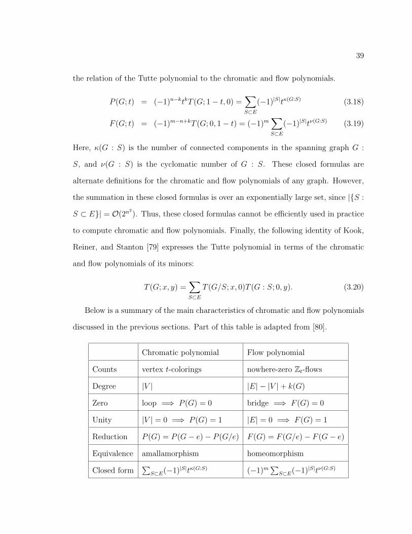
Below is a summary of the main characteristics of chromatic and flow polynomials
discussed in the previous sections. Part of this table is adapted from [80].
Chromatic polynomial Flow polynomial
Counts vertex t-colorings nowhere-zero Zt-flows
Degree |V | |E| − |V |+ k(G)
Zero loop =⇒ P (G) = 0 bridge =⇒ F (G) = 0
Unity |V | = 0 =⇒ P (G) = 1 |E| = 0 =⇒ F (G) = 1
Reduction P (G) = P (G− e)− P (G/e) F (G) = F (G/e)− F (G− e)
Equivalence amallamorphism homeomorphism
Closed form∑
S⊂E(−1)|S|tκ(G:S) (−1)m∑
S⊂E(−1)|S|tν(G:S)
40
Chapter 4
New results on chromatic polynomials
In this chapter, I introduce a low-order polynomial time algorithm for computing the
chromatic polynomials of generalized vertex joins of trees, and closed formulas for the
chromatic polynomials of generalized vertex joins of cycles and cliques. In the next
chapter, I will use the results obtained here together with graph duality and equation
3.17 to compute the flow polynomials of outerplanar graphs and generalized vertex
joins of cycles. In Chapter 6, these results are computationally compared against a
general-purpose solver.
4.1 Generalized vertex join trees
Let T = (V,E) be a tree with |V | = n, S be a multiset over V , and let TS be the
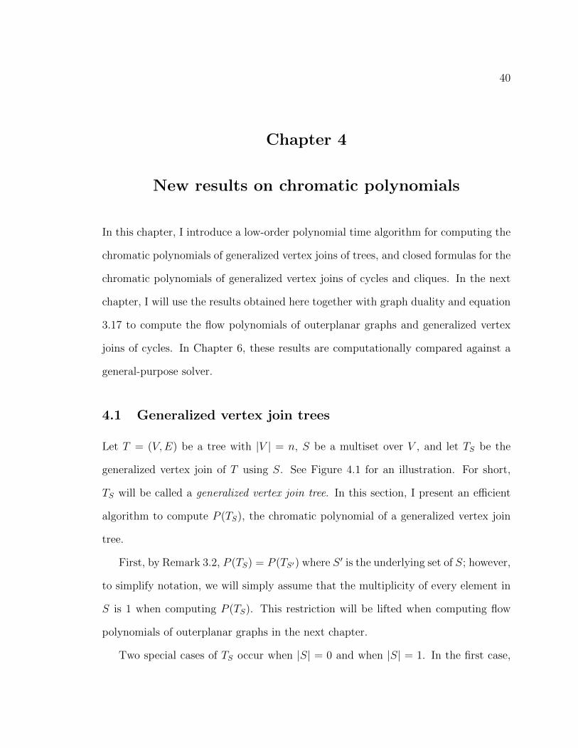
generalized vertex join of T using S. See Figure 4.1 for an illustration. For short,
TS will be called a generalized vertex join tree. In this section, I present an efficient
algorithm to compute P (TS), the chromatic polynomial of a generalized vertex join
tree.
First, by Remark 3.2, P (TS) = P (TS′) where S ′ is the underlying set of S; however,
to simplify notation, we will simply assume that the multiplicity of every element in
S is 1 when computing P (TS). This restriction will be lifted when computing flow
polynomials of outerplanar graphs in the next chapter.
Two special cases of TS occur when |S| = 0 and when |S| = 1. In the first case,
41
v*
Figure 4.1 : Forming a generalized vertex join tree TS from a given tree T and asubset of its nodes S.
TS consists of a tree on n vertices and an isolated vertex. Thus, by equations 3.4 and
3.10, P (TS) = t2(t − 1)n−1. In the second case, TS is a tree on n + 1 vertices, so by
equation 3.10, P (TS) = t(t− 1)n. Thus, from now on, we will assume that |S| ≥ 2.
Next, suppose there are b bridges in TS, and let B be the set of vertices in TS which
are an endpoint of some bridge, but do not belong to a cycle. Note that since |S| ≥ 2,
there is at least one cycle, so not all edges of TS are bridges. Let T ′S = TS −B. Using
(3.3), each bridge with a degree 1 endpoint can be separated from the rest of the
graph, adding a factor of P (K2)P (K1)
= t(t−1)t
to the chromatic polynomial of the resulting
graph; once every bridge in TS is removed, the resulting graph is T ′S and
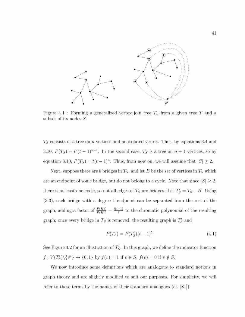
P (TS) = P (T ′S)(t− 1)b. (4.1)
See Figure 4.2 for an illustration of T ′S. In this graph, we define the indicator function
f : V (T ′S)\{v∗} → {0, 1} by f(v) = 1 if v ∈ S, f(v) = 0 if v /∈ S.
We now introduce some definitions which are analogous to standard notions in
graph theory and are slightly modified to suit our purposes. For simplicity, we will
refer to these terms by the names of their standard analogues (cf. [81]).
42
Figure 4.2 : Removing the bridges of TS to form T ′S.
First, select an arbitrary vertex r 6= v∗ in T ′S called a root. The level of a node in
T ′S is given by the function L : V (T ′S)\{v∗} → N∪{0} by L(v) = d(r, v), where d(r, v)
is the length of the shortest path between r and v in T ′S − v∗. Denote by Li(T′S) the
set of nodes at the ith level; more precisely, Li(T′S) = {v : L(v) = i}. Let L be the
height of T ′S, i.e, L = max{L(v) : v ∈ V (T ′S)\{v∗}}.
If L(v) = i, w is a child of v if w is adjacent to v and L(w) = i+ 1. Vertex z is a
descendant of v if z = v∗ or if there is a path v, p1, . . . , pr, z such that L(v) < L(p1) <
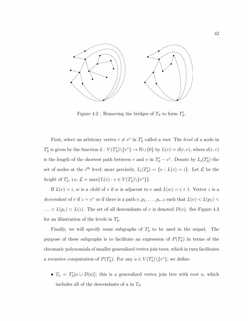
. . . < L(pr) < L(z). The set of all descendants of v is denoted D(v). See Figure 4.3
for an illustration of the levels in T ′S.
Finally, we will specify some subgraphs of T ′S to be used in the sequel. The
purpose of these subgraphs is to facilitate an expression of P (T ′S) in terms of the
chromatic polynomials of smaller generalized vertex join trees, which in turn facilitates
a recursive computation of P (T ′S). For any a ∈ V (T ′S)\{v∗}, we define:
• Ta = T ′S[a ∪ D(a)]; this is a generalized vertex join tree with root a, which
includes all of the descendants of a in TS.

43
v*
r
L0(T'S)
L1(T'S)
L2(T'S)
L3(T'S)
L4(T'S)
v*
r
a2
a1
Figure 4.3 : Selecting a node r and finding L(v) and Li(T′S).
• Tc = T ′S[{a} ∪ {c} ∪ D(c)]; this is a generalized vertex join tree with root a,
which includes only the descendants of c in TS.
• Ha = Ta/av∗; this is essentially a generalized vertex join of a forest with root a:
since Ta− v∗ is a tree, Ta− v∗− a is a forest, and a is connected to some subset
of the other vertices.
• Hc = Tc/av∗, this is one ‘branch’ of the generalized vertex join forest Ha, and
is also a generalized vertex join tree with root c, which includes all of the
descendants of c in T ′S (possibly with an extra connection between c and v∗).
See Figure 4.4 for an illustration of these subgraphs.
With this in mind, let a 6= v∗ be a vertex with children c1, . . . , ck, and suppose we
know P (Tci) and P (Hci) for 1 ≤ i ≤ k. Let I = {i : f(ci) = 1} and Z = {i : f(ci) = 0}
be the sets of children of a which are connected and not connected to v∗, respectively.
Then, we can compute P (Ha) as follows.

44
a2
a2a1a1
Figure 4.4 : From left to right: Ta1 ; Ta1 ; Ha2 ; Ha2 , for two vertices a1 and a2 of thegraph T ′S shown in Figure 4.3, right.
P (Ha) =1
tk−1
k∏i=1
P (Hci)
=1
tk−1
∏I
P (Hci)∏Z
P (Hci)
=1
tk−1
∏I
P (Tci)∏Z
(P (Tci)− P (Hci)
)Here, the first equality follows from (3.3) and the definition of Hci , since Hc1 , . . . , Hck
all have only the vertex a in common. The second equality is obtained by partitioning
{1, . . . , k} into I and Z. Finally, if a was originally connected to v∗, then Hci =
Tci ; otherwise, the deletion-contraction formula (3.2) yields P (Hci) = P (Hci − ac)−
P (Hci/ac) = P (Tci)− P (Hci), and the third equality follows.
Next, we compute P (Ta) by considering two cases: a is either in S or not. Let
P1(Ta) = P (Ta), where f(a) = 1, and P0(Ta) = P (Ta), where f(a) = 0. Clearly,
P (Ta) = f(a)P1(Ta) +(1 − f(a)
)P0(Ta). We now find P1(Ta) and P0(Ta) separately
as follows.
45
P1(Ta) =1(
t(t− 1))k−1 k∏
i=1
P (Tci)
=1(
t(t− 1))k−1 ∏
I
P (Tci)∏Z
P (Tci)
=
∏I
(P (Tci)(t− 2)
)(t(t− 1)
)k−1 ∏Z
(P (Tci + civ
∗) + P (Tci/civ∗))
=
∏I
(P (Tci)(t− 2)
)(t(t− 1)
)k−1 ∏Z
(P (Tci + civ
∗)(t− 2) + P (Hci)(t− 1))
=
∏I
(P (Tci)(t− 2)
)(t(t− 1)
)k−1 ∏Z
((P (Tci)− P (Hci)
)(t− 2) + P (Hci)(t− 1)
)=
1(t(t− 1)
)k−1 ∏I
(P (Tci)(t− 2)
)∏Z
((t− 2)P (Tci) + P (Hci)
)P0(Ta) = P (Ta + av∗) + P (Ta/av
∗) = P1(Ta) + P (Ha)
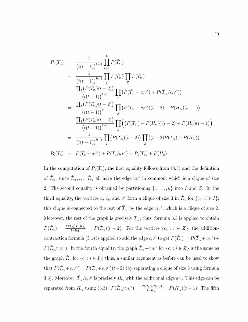
In the computation of P1(Ta), the first equality follows from (3.3) and the definition
of Tci , since Tc1 , . . . , Tck all have the edge av∗ in common, which is a clique of size
2. The second equality is obtained by partitioning {1, . . . , k} into I and Z. In the
third equality, the vertices a, ci, and v∗ form a clique of size 3 in Tci for {ci : i ∈ I};
this clique is connected to the rest of Tci by the edge civ∗, which is a clique of size 2.
Moreover, the rest of the graph is precisely Tci ; thus, formula 3.3 is applied to obtain
P (Tci) =P (Tci )P (K3)
P (K2)= P (Tci)(t − 2). For the vertices {ci : i ∈ Z}, the addition-
contraction formula (3.1) is applied to add the edge civ∗ to get P (Tci) = P (Tci+civ
∗)+
P (Tci/civ∗). In the fourth equality, the graph Tci + civ
∗ for {ci : i ∈ Z} is the same as
the graph Tci for {ci : i ∈ I}; thus, a similar argument as before can be used to show
that P (Tci +civ∗) = P (Tci +civ
∗)(t−2) (by separating a clique of size 3 using formula
3.3). Moreover, Tci/civ∗ is precisely Hci with the additional edge aci. This edge can be
separated from Hci using (3.3): P (Tci/civ∗) =
P (Hci )P (K2)
P (K1)= P (Hci)(t− 1). The fifth
46
equality follows from the deletion-contraction formula (3.2) applied to the edge civ∗,
so that P (Tci + civ∗) = P (Tci + civ
∗− civ∗)−P ((Tci + civ∗)/civ
∗) = P (Tci)−P (Hci).
Finally, the last equality is obtained by simple algebraic manipulations.
In the computation of P0(Ta), the first equality follows from the addition contrac-
tion formula (3.1), as the edge av∗ is added. Then, by the definitions of P1 and Ha,
P (Ta + av∗) = P1(Ta) and P (Ta/av∗) = P (Ha) and the second equality follows.
Thus, I have shown how to express P (Ta) and P (Ha) in terms of P (Tci) and
P (Hci), 1 ≤ i ≤ k. Using these identities, I propose the following algorithm for
finding the chromatic polynomial of a generalized vertex join tree TS.
Algorithm 1
1. Find and remove the bridges of TS to acquire T ′S
2. For i = L to 0
Compute P (Ta) and P (Ha) for each a ∈ Li(T ′S)
3. Compute P (TS) using (4.1)
Theorem 4.1
Algorithm 1 finds the correct chromatic polynomial of a generalized vertex join tree
TS using O(n2 log n) time and O(n) space.
Proof 4.1 It was shown in (4.1) and the preceding discussion that by finding the
bridges of TS and the chromatic polynomial of T ′S, P (TS) can be easily computed as
well. Thus, we only need to verify that Step 2 of the algorithm correctly computes
P (T ′S).
47
It was already established that for every a ∈ V (T ′S)\{v∗}, P (Ta) and P (Ha) can
be expressed in terms of P (Tc) and P (Hc) for every child c of a. Note that this
expression is trivially satisfied for vertices which have no children. By construction,
vertices in LL(T ′S) have no children, so P (Ta) and P (Ha) can be found immediately
for any vertex a ∈ LL(T ′S). For L > i ≥ 0, a vertex a in Li(T′S) either has no children,
or has all of its children in Li+1(T′S). In either case, P (Tc) and P (Hc) are known for
every child c of a — either vacuously or inductively. Thus, P (Ta) and P (Ha) can also
be computed using the formulas derived earlier in this section. Since by construction,
P (T ′S) = P (Tr) and L0(T′S) = {r}, Algorithm 1 indeed finds the correct chromatic
polynomial of TS.
To verify the time-complexity of the algorithm, let |V (T )| = n. The bridges in TS
and the graph T ′S can be found in O(n2) time∗ by successively finding and deleting
degree 1 vertices of TS. Also, the level and list of children of each vertex of T ′S − v∗
can be found with O(n) time by a breadth-first scan.
Each evaluation of P (Ta) and P (Ha) requires the multiplication of O(ak) polyno-
mials, where ak is the number of children of a. Since we evaluate P (Ta) and P (Ha)
for O(n) vertices, and the total number of children in T ′S is O(n), the evaluation of
P (T ′S) requires the multiplication of O(n) polynomials. Each of these polynomials
has degree at most O(n), since P (T ′S) has degree O(n). The time-complexity of mul-
tiplying two polynomials of degree n, using a Fast Fourier Transform, is O(n log n),
so the total time complexity of Algorithm 1 is O(n2 log n).
Finally, to verify the space-complexity, note that the total number of vertices in
the set of graphs {Ta, Ha : a ∈ Li(T ′S)} is at most O(n). Recall that the chromatic
∗By the restriction that every element in S has multiplicity 1, |E(TS)| = O(n). Thus, using the
algorithm of Tarjan [81], all bridges of TS can actually be found in O(n) time.
48
polynomial of a graph with k vertices has degree k; hence, the sum of the degrees of
the set of polynomials {P (Ta), P (Ha) : a ∈ Li(T′S)} is O(n). A set of polynomials
whose degrees add up to n can be stored with O(n) space. Thus, since we only have
to store the polynomials P (Ta) and P (Ha) for a in one level at a time, the total
space-complexity of Algorithm 1 is O(n). �
4.2 Generalized vertex join cycles
Let C = (V,E) be a cycle, S be a multiset over V and let CS be the generalized
vertex join of C using S. For short, CS will be called a generalized vertex join cycle.
In the literature, graphs of a similar form have also been called “generalized wheel”
graphs, and have been investigated by other approaches and in different contexts (cf.
[82, 80, 40]). In the remainder of this section and in Section 5.2, I will present closed
formulas for P (CS) and F (CS) in a unified framework.
Suppose the generalized vertex join cycle CS is equipped with a “wheel” plane
embedding obtained by placing v∗ in the bounded face of a plane drawing of C,
and drawing edges from the vertices in S to v∗ so that the resulting graph remains
plane. Since cycles have a unique plane embedding, the “wheel” embedding of CS is
unique up to topological conjugacy. Moreover, since chromatic and flow polynomials
are independent of embedding, this embedding can be considered without loss of
generality. The vertices along the outer face of CS will be labeled in clockwise order
as v1, . . . , vn; see Figure 4.5 for an illustration. The edges incident to v∗ will be called
spokes.
If S = ∅, then by equation 3.11, P (CS) = tP (Cn) = t((t − 1)n + (−1)n(t − 1)
);
thus, suppose hereafter that S 6= ∅ and consider S ′, the underlying set of S. By
(3.7), P (CS) = P (CS′). Without loss of generality, suppose that S ′ = {va1 , . . . , vas}
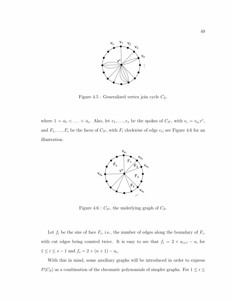
49
v*
v1 v2v3
...
v4
vn
Figure 4.5 : Generalized vertex join cycle CS.
where 1 = a1 < . . . < as. Also, let e1, . . . , es be the spokes of CS′ , with ei = vaiv∗,
and F1, . . . , Fs be the faces of CS′ , with Fi clockwise of edge ei; see Figure 4.6 for an
illustration.
v*
va1va2
vas
...
va3
va4
F1F2
F3
F4
Fs
Figure 4.6 : CS′ , the underlying graph of CS.
Let fi be the size of face Fi, i.e., the number of edges along the boundary of Fi,
with cut edges being counted twice. It is easy to see that fi = 2 + ai+1 − ai for
1 ≤ i ≤ s− 1 and fs = 2 + (n+ 1)− as.
With this in mind, some auxiliary graphs will be introduced in order to express
P (CS) as a combination of the chromatic polynomials of simpler graphs. For 1 ≤ i ≤
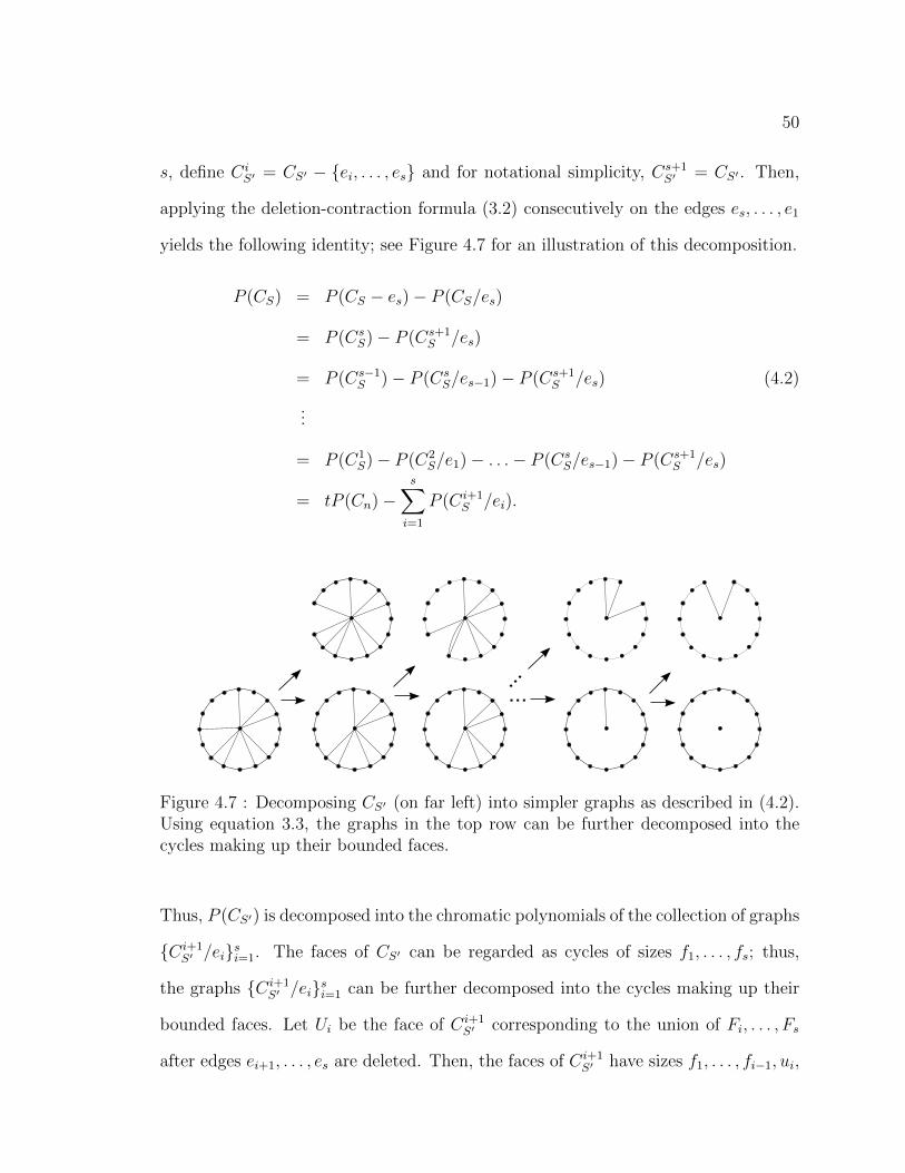
50
s, define CiS′ = CS′ − {ei, . . . , es} and for notational simplicity, Cs+1
S′ = CS′ . Then,
applying the deletion-contraction formula (3.2) consecutively on the edges es, . . . , e1
yields the following identity; see Figure 4.7 for an illustration of this decomposition.
P (CS) = P (CS − es)− P (CS/es)
= P (CsS)− P (Cs+1
S /es)
= P (Cs−1S )− P (Cs
S/es−1)− P (Cs+1S /es) (4.2)
...
= P (C1S)− P (C2
S/e1)− . . .− P (CsS/es−1)− P (Cs+1
S /es)
= tP (Cn)−s∑i=1
P (Ci+1S /ei).
......
Figure 4.7 : Decomposing CS′ (on far left) into simpler graphs as described in (4.2).Using equation 3.3, the graphs in the top row can be further decomposed into thecycles making up their bounded faces.
Thus, P (CS′) is decomposed into the chromatic polynomials of the collection of graphs
{Ci+1S′ /ei}si=1. The faces of CS′ can be regarded as cycles of sizes f1, . . . , fs; thus,
the graphs {Ci+1S′ /ei}si=1 can be further decomposed into the cycles making up their
bounded faces. Let Ui be the face of Ci+1S′ corresponding to the union of Fi, . . . , Fs
after edges ei+1, . . . , es are deleted. Then, the faces of Ci+1S′ have sizes f1, . . . , fi−1, ui,
51
where ui is the size of Ui; more precisely,
ui = 2 + (fi − 2) + . . .+ (fs − 2)
= 2 + (−2)(s− i+ 1) +s∑j=i
fj (4.3)
= 2(i− s) +s∑j=i
fj.
Let Ji be the multiset of sizes of faces of Ci+1S′ /ei, i.e., J1 = {n} and for 2 ≤ i ≤ s,
Ji = {f1, . . . , fi−2, fi−1 − 1, ui − 1}. (4.4)
Then, starting from a face of Ci+1S′ /ei which borders the contracted edge, and using
the fact that this face shares just one edge (which is a clique of size 2) with the
rest of the graph, formula 3.3 can be successively applied to decompose Ci+1S /ei into
cycles with sizes in Ji in order to evaluate P (Ci+1S′ /ei). In particular, P (Ci+1
S′ /ei) =
P (K2)1−i∏
j∈Ji P (Cj). Thus, by (4.2) we have
P (CS) = P (CS′) = tP (Cn)−s∑i=1
∏j∈Ji P (Cj)
P (K2)i−1(4.5)
= t((t− 1)n + (−1)n(t− 1))−s∑i=1
∏j∈Ji((t− 1)j + (−1)j(t− 1))
(t(t− 1))i−1.
Note that formula (4.5) depends only on the sequence of face-sizes of CS′ and hence
only on S.
4.3 Generalized vertex join cliques
Let K = (V,E) be a complete graph, S be a multiset over V and let KS be the
generalized vertex join of K using S. For short, we will call KS a generalized vertex
join clique. Let |V | = n, S ′ be the underlying set of S, and |S ′| = s. Then,
52
P (KS) = P (KS′) =P (Kn)P (Ks+1)
P (Ks)= (t− s)
n−1∏i=0
(t− i), (4.6)
where the first equality follows from equation 3.7, the second follows from (3.3) —
since KS′ [S ′ ∪ {v∗}] = Ks+1, and the third follows from equation 3.9.
Since in general complete graphs are not planar, graph duality cannot be applied
to generalized vertex join cliques to obtain a result about flow polynomials. However,
it would be interesting to investigate the flow polynomials of generalized vertex join
cliques directly. This will likely be a challenging task: Tutte [8] derived a formula
and a generating function for the flow polynomial of a complete graph which is quite
complicated; adding a vertex with arbitrary connections to the others will complicate
this formula even more. Such investigations will be the focus of future work.
53
Chapter 5
New results on flow polynomials
In this chapter, I show that the family of outerplanar graphs is dual to the family
of generalized vertex join trees. Thus, Algorithm 1 from Chapter 4 can be adapted
to compute the flow polynomials of outerplanar graphs. I also show that the family
of generalized vertex join cycles is self-dual, so formula 4.5 from Chapter 4 can be
transformed into a closed formula for computing the flow polynomials of generalized
vertex join cycles.
5.1 Outerplanar graphs
Let B be a biconnected outerplane graph with bounded faces F1, . . . , Fs and outer
face F∗. The weak dual of B is a tree T = (V,E), where vertex vi ∈ T corresponds
to face Fi ∈ B (see [83] for more details). Suppose Fi shares fi edges with F∗, and
let v∗ be the vertex in the dual of B corresponding to F∗. Then, the dual of B is the
generalized vertex join tree TS, where S is the multiset over V in which vi appears fi
times.
With this in mind, the flow polynomial of an arbitrary outerplanar graph G can
be computed by applying Algorithm 1 to the dual of each biconnected component of
G. This procedure is formally outlined in Algorithm 2 below.
54
Algorithm 2
1. Find the biconnected components G1, . . . , Gk of G
2. Find the dual graphs G∗1, . . . , G∗k
3. Compute P (G∗1), . . . , P (G∗k) using Algorithm 1
4. Compute F (G) by F (G) = 1tk
∏ki=1 P (G∗i )
Theorem 5.1
Algorithm 2 finds the correct flow polynomial of an outerplanar graph G using
O(n2 log n) time and O(n) space.
Proof 5.1 Consider the biconnected components of G as separate graphs, i.e., Gi =
G[Vi] where Vi is a maximal subset of V (G) such that G[Vi] is biconnected. Then,
each Gi is a biconnected outerplanar graph and by (3.16) and (3.17),
F (G) =k∏i=1
F (Gi) =1
tk
k∏i=1
P (G∗i ).
Since the dual of a biconnected outerplanar graph is a generalized vertex join tree,
Algorithm 1 can be used to compute P (G∗i ) for 1 ≤ i ≤ k, so Algorithm 2 indeed
finds the correct flow polynomial of G.
To verify the time- and space-complexity, let |V (G)| = n and |V (Gi)| = ni;
clearly n1 + . . . + nk = O(n). By the algorithms of Hopcroft and Tarjan [84, 85],
the biconnected components G1, . . . , Gk of G can be found, embedded in the plane,
and have their dual graphs G∗1, . . . , G∗k computed, with O(n) time and space. Finally,
note that Algorithm 1 runs with O(n2i log ni) time on the generalized vertx join tree
55
G∗i and that
k∑i=1
(n2i log ni
)≤
(k∑i=1
ni
)2
log
(k∑i=1
ni
)= O(n2 log n).
Hence, Algorithm 1 can be applied to find P (G∗1), . . . , P (G∗k) in O(n2 log n) time and
O(n) space. Thus, the total time complexity of Algorithm 2 is O(n2 log n) and the
total space complexity is O(n). �
I conclude this section with a characterization of the duality between outerplanar
graphs and generalized vertex join trees.
Proposition 5.1
Let G be a simple biconnected outerplane graph and TS be its dual generalized vertex
join tree. G is simple if and only if every vertex of TS has degree at least 3.
Proof 5.2 Suppose G is a simple biconnected outerplane graph. G has no parallel
edges or loops, so G has no faces of size 1 or 2. Thus, each face of G is incident to at
least 3 edges, so each vertex of TS has degree at least 3.
Now, suppose TS is a generalized vertex join tree, and that every vertex of TS has
degree at least 3. We will show that TS is the dual of a simple biconnected outerplanar
graph by induction on the number of vertices of TS. If TS has two vertices v and v∗,
all the edges in TS must join v to v∗ since by construction, TS can have no loops.
Thus, TS is the dual of some cycle of size at least 3 (which is simple, biconnected,
and outerplanar). Next, let TS be a generalized vertex join tree on k + 1 vertices
with minimum vertex degree at least 3, and let v be a leaf of T . Since T is a tree, v
has a unique neighbor u in T with exactly one edge between u and v. Moreover, by
assumption, v must be connected to v∗ by ` ≥ 2 edges and u must be incident to at
least two edges other than uv. Thus, if we delete v from TS and add an edge from u
to v∗, we obtain a generalized vertex join tree on k vertices, which by induction is the
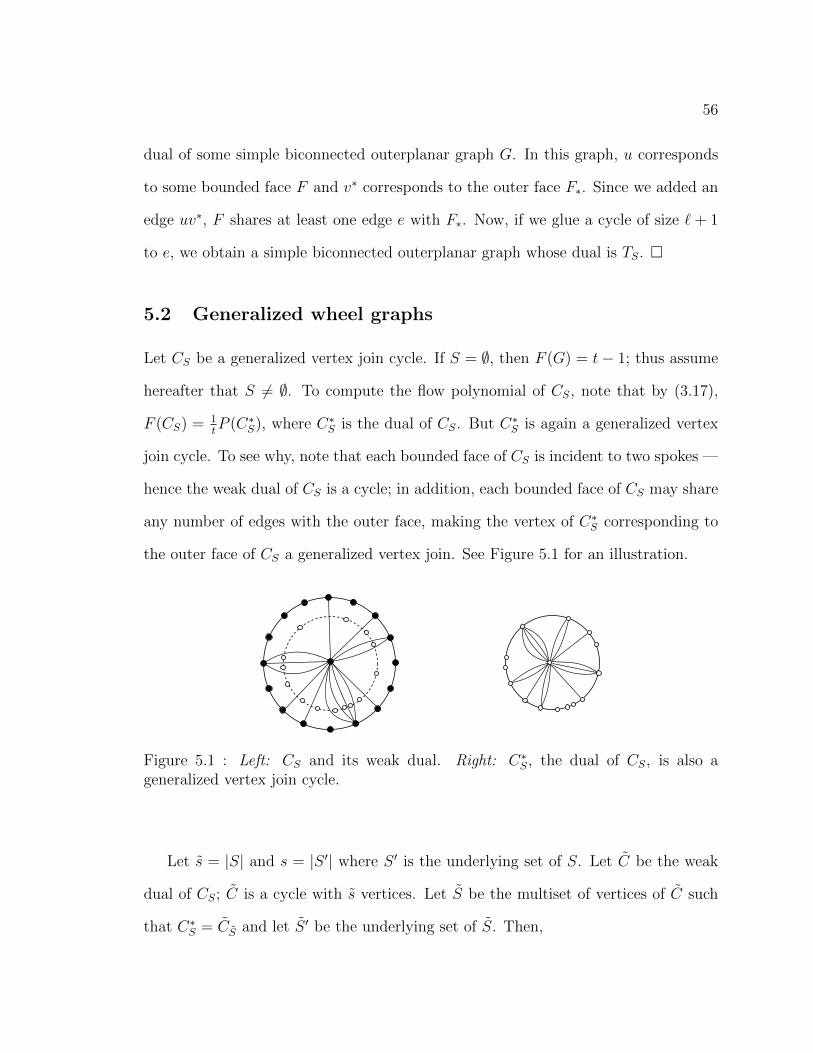
56
dual of some simple biconnected outerplanar graph G. In this graph, u corresponds
to some bounded face F and v∗ corresponds to the outer face F∗. Since we added an
edge uv∗, F shares at least one edge e with F∗. Now, if we glue a cycle of size ` + 1
to e, we obtain a simple biconnected outerplanar graph whose dual is TS. �
5.2 Generalized wheel graphs
Let CS be a generalized vertex join cycle. If S = ∅, then F (G) = t− 1; thus assume
hereafter that S 6= ∅. To compute the flow polynomial of CS, note that by (3.17),
F (CS) = 1tP (C∗S), where C∗S is the dual of CS. But C∗S is again a generalized vertex
join cycle. To see why, note that each bounded face of CS is incident to two spokes —
hence the weak dual of CS is a cycle; in addition, each bounded face of CS may share
any number of edges with the outer face, making the vertex of C∗S corresponding to
the outer face of CS a generalized vertex join. See Figure 5.1 for an illustration.
Figure 5.1 : Left: CS and its weak dual. Right: C∗S, the dual of CS, is also ageneralized vertex join cycle.
Let s = |S| and s = |S ′| where S ′ is the underlying set of S. Let C be the weak
dual of CS; C is a cycle with s vertices. Let S be the multiset of vertices of C such
that C∗S = CS and let S ′ be the underlying set of S. Then,
57
F (CS) =1
tP (C∗S) =
1
tP (CS) =
1
tP (CS′). (5.1)
It is easy to see that CS′ and CS′ have the same number of faces. Moreover,
if f1 . . . , fs are the sizes of the faces of CS′ in clockwise order, then fi equals the
multiplicity of vai in S plus 2. Thus, to find F (CS), we simply plug in the sequence
of face-sizes of C∗S into (4.3), (4.4), and (4.5) as follows:
F (CS) = (t− 1)s + (−1)s(t− 1)− 1
t
s∑i=1
∏j∈Ji((t− 1)j + (−1)j(t− 1))
(t(t− 1))i−1,
where J1 = {s} and Ji = {f1, . . . , fi−2, fi−1 − 1, 2(i− s) +∑s
j=i fj − 1} for 2 ≤ i ≤ s.
Note that this closed formula again depends only on S, since the face-sizes of C∗S are
determined from S.
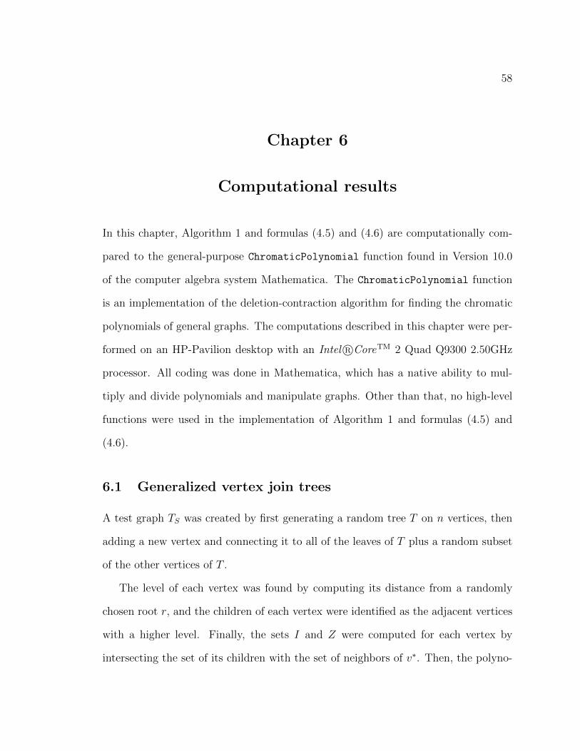
58
Chapter 6
Computational results
In this chapter, Algorithm 1 and formulas (4.5) and (4.6) are computationally com-
pared to the general-purpose ChromaticPolynomial function found in Version 10.0
of the computer algebra system Mathematica. The ChromaticPolynomial function
is an implementation of the deletion-contraction algorithm for finding the chromatic
polynomials of general graphs. The computations described in this chapter were per-
formed on an HP-Pavilion desktop with an Intel R©CoreTM 2 Quad Q9300 2.50GHz
processor. All coding was done in Mathematica, which has a native ability to mul-
tiply and divide polynomials and manipulate graphs. Other than that, no high-level
functions were used in the implementation of Algorithm 1 and formulas (4.5) and
(4.6).
6.1 Generalized vertex join trees
A test graph TS was created by first generating a random tree T on n vertices, then
adding a new vertex and connecting it to all of the leaves of T plus a random subset
of the other vertices of T .
The level of each vertex was found by computing its distance from a randomly
chosen root r, and the children of each vertex were identified as the adjacent vertices
with a higher level. Finally, the sets I and Z were computed for each vertex by
intersecting the set of its children with the set of neighbors of v∗. Then, the polyno-
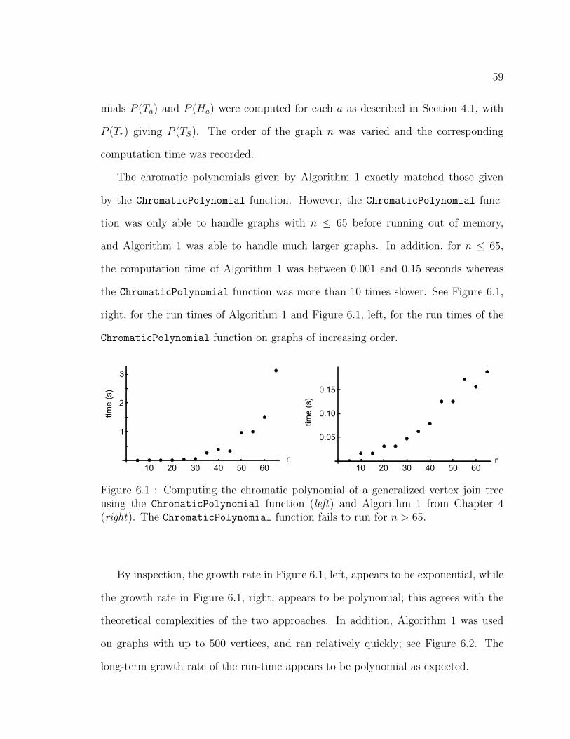
59
mials P (Ta) and P (Ha) were computed for each a as described in Section 4.1, with
P (Tr) giving P (TS). The order of the graph n was varied and the corresponding
computation time was recorded.
The chromatic polynomials given by Algorithm 1 exactly matched those given
by the ChromaticPolynomial function. However, the ChromaticPolynomial func-
tion was only able to handle graphs with n ≤ 65 before running out of memory,
and Algorithm 1 was able to handle much larger graphs. In addition, for n ≤ 65,
the computation time of Algorithm 1 was between 0.001 and 0.15 seconds whereas
the ChromaticPolynomial function was more than 10 times slower. See Figure 6.1,
right, for the run times of Algorithm 1 and Figure 6.1, left, for the run times of the
ChromaticPolynomial function on graphs of increasing order.
time
(s)
3
2
1
10 20 30 40 50 60n
10 20 30 40 50 60n
0.05
0.10
0.15
time
(s)
Figure 6.1 : Computing the chromatic polynomial of a generalized vertex join treeusing the ChromaticPolynomial function (left) and Algorithm 1 from Chapter 4(right). The ChromaticPolynomial function fails to run for n > 65.
By inspection, the growth rate in Figure 6.1, left, appears to be exponential, while
the growth rate in Figure 6.1, right, appears to be polynomial; this agrees with the
theoretical complexities of the two approaches. In addition, Algorithm 1 was used
on graphs with up to 500 vertices, and ran relatively quickly; see Figure 6.2. The
long-term growth rate of the run-time appears to be polynomial as expected.
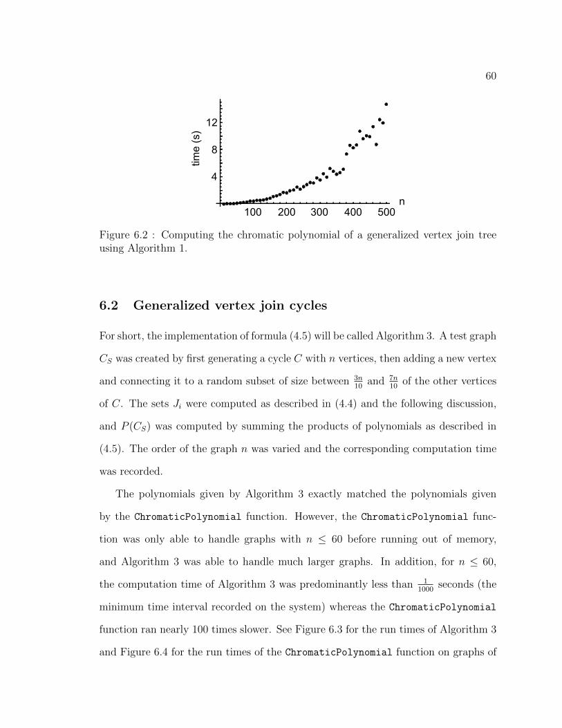
60
4
8
12
100 200 300 400 500
time
(s)
n
Figure 6.2 : Computing the chromatic polynomial of a generalized vertex join treeusing Algorithm 1.
6.2 Generalized vertex join cycles
For short, the implementation of formula (4.5) will be called Algorithm 3. A test graph
CS was created by first generating a cycle C with n vertices, then adding a new vertex
and connecting it to a random subset of size between 3n10
and 7n10
of the other vertices
of C. The sets Ji were computed as described in (4.4) and the following discussion,
and P (CS) was computed by summing the products of polynomials as described in
(4.5). The order of the graph n was varied and the corresponding computation time
was recorded.
The polynomials given by Algorithm 3 exactly matched the polynomials given
by the ChromaticPolynomial function. However, the ChromaticPolynomial func-
tion was only able to handle graphs with n ≤ 60 before running out of memory,
and Algorithm 3 was able to handle much larger graphs. In addition, for n ≤ 60,
the computation time of Algorithm 3 was predominantly less than 11000
seconds (the
minimum time interval recorded on the system) whereas the ChromaticPolynomial
function ran nearly 100 times slower. See Figure 6.3 for the run times of Algorithm 3
and Figure 6.4 for the run times of the ChromaticPolynomial function on graphs of
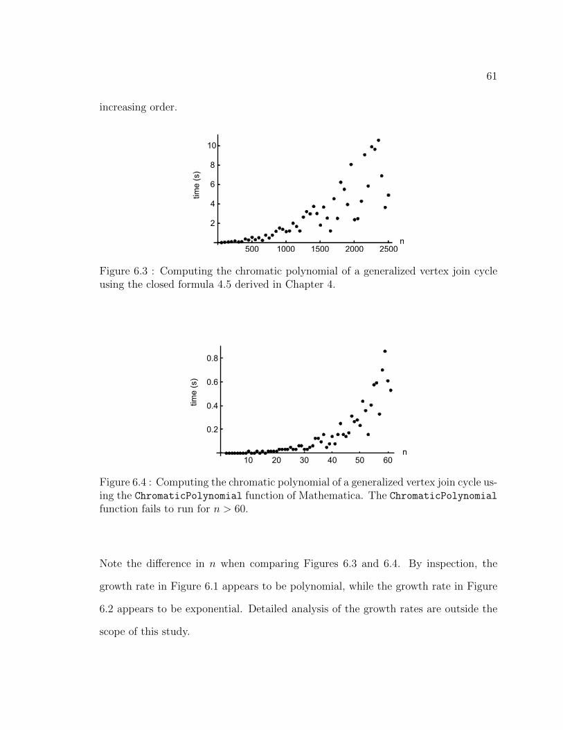
61
increasing order.
time
(s)
n
10
8
6
4
2
500 1000 1500 2000 2500
Figure 6.3 : Computing the chromatic polynomial of a generalized vertex join cycleusing the closed formula 4.5 derived in Chapter 4.
n
time
(s)
10 20 30 40 50 60
0.2
0.4
0.6
0.8
Figure 6.4 : Computing the chromatic polynomial of a generalized vertex join cycle us-ing the ChromaticPolynomial function of Mathematica. The ChromaticPolynomialfunction fails to run for n > 60.
Note the difference in n when comparing Figures 6.3 and 6.4. By inspection, the
growth rate in Figure 6.1 appears to be polynomial, while the growth rate in Figure
6.2 appears to be exponential. Detailed analysis of the growth rates are outside the
scope of this study.
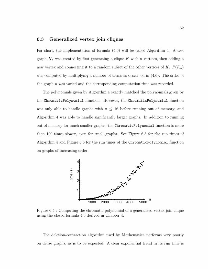
62
6.3 Generalized vertex join cliques
For short, the implementation of formula (4.6) will be called Algorithm 4. A test
graph KS was created by first generating a clique K with n vertices, then adding a
new vertex and connecting it to a random subset of the other vertices of K. P (KS)
was computed by multiplying a number of terms as described in (4.6). The order of
the graph n was varied and the corresponding computation time was recorded.
The polynomials given by Algorithm 4 exactly matched the polynomials given by
the ChromaticPolynomial function. However, the ChromaticPolynomial function
was only able to handle graphs with n ≤ 16 before running out of memory, and
Algorithm 4 was able to handle significantly larger graphs. In addition to running
out of memory for much smaller graphs, the ChromaticPolynomial function is more
than 100 times slower, even for small graphs. See Figure 6.5 for the run times of
Algorithm 4 and Figure 6.6 for the run times of the ChromaticPolynomial function
on graphs of increasing order.
1000 2000 3000 4000 5000
1
2
3
4
n
time
(s)
Figure 6.5 : Computing the chromatic polynomial of a generalized vertex join cliqueusing the closed formula 4.6 derived in Chapter 4.
The deletion-contraction algorithm used by Mathematica performs very poorly
on dense graphs, as is to be expected. A clear exponential trend in its run time is

63
5 10 15
50
100
150
200
ntim
e (s
)
Figure 6.6 : Computing the chromatic polynomial of a generalized vertex join cliqueusing the ChromaticPolynomial function of Mathematica. The program fails to runfor n ≥ 16.
exhibited in Figure 6.6; moreover the function fails for generalized vertex join cliques
with more than 16 vertices. On the other hand, Algorithm 4 is much faster, is able to
handle graphs with thousands of vertices in less than 5 seconds, and has a polynomial
growth rate as can be seen from Figure 6.5.
6.4 Discussion
All three computational experiments reveal that my algorithms were much faster than
the ChromaticPolynomial function and able to handle much larger graphs from the
appropriate family. This is not surprising, since generality is often achieved at the
expense of speed. However, this motivates the inclusion of a preprocessing step in
general purpose algorithms: if a general graph is suspected to contain one or more
subgraphs whose chromatic polynomials can be found efficiently, it may be worth to
locate those subgraphs and modify the deletion-contraction algorithm so that they
appear as components in some step of the recursion. This will remove a large part of
the recursion tree and may speed up the computation of the chromatic polynomial
64
significantly.
Finally, note that simply having a closed formula for a chromatic polynomial
does not mean it can be used efficiently. For instance, recall from Chapter 3 that
the chromatic polynomial of any graph G = (V,E) can be computed by the closed
formula P (G; t) =∑
S⊂E(−1)|S|tκ(G:S), where κ(G : S) is the number of connected
components in the graph (V, S). However, this formula requires, among other things,
a summation with an exponential number of terms. In contrast, formulas 4.5 and
4.6 (and Algorithm 1) can be used in polynomial time in practice, as seen from the
preceding experiments.
65
Chapter 7
Conclusion
This thesis gave an overview of chromatic and flow polynomials, and presented new
efficient methods to compute these polynomials on specific families of graphs. The
presented methods were validated by computational results. In particular, a low-order
polynomial time algorithm for computing the chromatic polynomials of generalized
vertex join trees was presented; this algorithm was also adapted to find the flow
polynomials of outerplanar graphs. In addition, closed formulas were derived for
the chromatic polynomials of generalized vertex join cliques, and the chromatic and
flow polynomials of generalized vertex join cycles. My experiments showed that com-
putation based on the proposed formulas and algorithms strongly outperforms the
general-purpose deletion-contraction algorithm used by Mathematica on the consid-
ered families of graphs. The novel theoretical results presented in this thesis appear
in [86].
Applications of chromatic and flow polynomials to statistical physics, combina-
torics, theoretical computer science, and other branches of graph theory were dis-
cussed throughout this thesis. In addition, the chromatic and flow polynomials of a
graph count the number of ways to color and assign flow to the graph; their roots,
coefficients, derivatives, and values at specific points contain other important infor-
mation and are of independent interest.
Unfortunately, these graph polynomials are generally difficult to compute; thus,
research in this area has focused on exploiting the structure of specific families of

66
graphs in order to characterize their chromatic and flow polynomials. There are a
number of simple graphs whose chromatic polynomials are being sought. Of note is
the problem of efficiently finding the chromatic polynomial of an m × n grid graph,
which is largely still unsolved. Grid graphs may have arbitrarily large treewidth,
which renders bounded-treewidth algorithms like the ones discussed in Chapter 3
inapplicable. In the words of Read and Tutte, “that is an easy question to ask, but
without a doubt a fiendishly difficult one to answer” [56].
The generalized vertex join operation provides a natural extension to all families
of graphs; thus, future work may focus on finding closed formulas for the chromatic
polynomials of generalized vertex joins of various families of graphs whose chromatic
polynomials are already known, such as star graphs, helm graphs, and sun graphs.
Additionally, the chromatic polynomials of graphs obtained by a sequence of gen-
eralized vertex joins may also be of interest. In particular, multiple vertex joins of
cliques are a promising start. Of course, one cannot expect too much: any loopless
graph on n vertices can be obtained through a sequence of n − 1 vertex joins start-
ing from a single vertex, so an efficient formula or algorithm cannot be expected for
an arbitrarily long sequence of generalized vertex joins. However, for short enough
sequences, useful results may be obtained.
This also motivates preprocessing in general purpose algorithms. If a general
graph is suspected to contain one or more subgraphs whose chromatic or flow polyno-
mials can be found efficiently, locating those subgraphs and modifying the deletion-
contraction algorithm so that they appear as components in some step of the recursion
may speed up the computation of the chromatic and flow polynomials significantly.
67
Bibliography
[1] N. Biggs, Algebraic Graph Theory. Cambridge University Press, 1993.
[2] C. D. Godsil, G. Royle, and C. Godsil, Algebraic Graph Theory, vol. 207. Springer
New York, 2001.
[3] Mishyp, “Map clip art.” Clker.com, 2011.
[4] G. D. Birkhoff, “A determinant formula for the number of ways of coloring a
map,” The Annals of Mathematics, vol. 14, no. 1/4, pp. 42–46, 1912.
[5] K. I. Appel and W. Haken, Every planar map is four colorable, vol. 98. American
Mathematical Society, Providence, 1989.
[6] H. Whitney, “A logical expansion in mathematics,” Bulletin of the American
Mathematical Society, vol. 38, no. 8, pp. 572–579, 1932.
[7] W. T. Tutte, “A contribution to the theory of chromatic polynomials,” Canad.
J. Math, vol. 6, no. 80-91, pp. 3–4, 1954.
[8] W. T. Tutte, “On dichromatic polynomials,” Journal of Combinatorial Theory,
vol. 2, no. 3, pp. 301–320, 1967.
[9] C. Hoede and X. Li, “Clique polynomials and independent set polynomials of
graphs,” Discrete Mathematics, vol. 125, no. 1, pp. 219–228, 1994.
68
[10] B. McClosky, A. Simms, and I. V. Hicks, “Co-2-plex polynomials,” Journal of
Combinatorial Optimization, vol. 22, no. 4, pp. 640–650, 2011.
[11] G. Chia, “A bibliography on chromatic polynomials,” Discrete Mathematics,
vol. 172, no. 1, pp. 175–191, 1997.
[12] R. C. Read, “An introduction to chromatic polynomials,” Journal of Combina-
torial Theory, vol. 4, no. 1, pp. 52–71, 1968.
[13] M. Kubale, Graph Colorings, vol. 352. American Mathematical Soc., 2004.
[14] A. D. Sokal, “Chromatic polynomials, Potts models and all that,” Physica A:
Statistical Mechanics and its Applications, vol. 279, no. 1, pp. 324–332, 2000.
[15] A. D. Sokal, “The multivariate Tutte polynomial (alias Potts model) for graphs
and matroids,” Surveys in combinatorics, vol. 327, pp. 173–226, 2005.
[16] C. Thomassen, “Chromatic roots and Hamiltonian paths,” Journal of Combina-
torial Theory, Series B, vol. 80, no. 2, pp. 218–224, 2000.
[17] A. Mohr and T. Porter, “Applications of chromatic polynomials involving stirling
numbers,” J. Combin. Math. Combin. Comput, vol. 70, pp. 57–64, 2009.
[18] E. G. Whitehead, “Stirling number identities from chromatic polynomials,” Jour-
nal of Combinatorial Theory, Series A, vol. 24, no. 3, pp. 314–317, 1978.
[19] S. Beraha, J. Kahane, and N. Weiss, “Limits of chromatic zeros of some families
of maps,” Journal of Combinatorial Theory, Series B, vol. 28, no. 1, pp. 52–65,
1980.
[20] W. Tutte, “On chromatic polynomials and the golden ratio,” Journal of Combi-
natorial Theory, vol. 9, no. 3, pp. 289–296, 1970.
69
[21] E. H. Lieb, “Residual entropy of square ice,” Physical Review, vol. 162, no. 1,
p. 162, 1967.
[22] L. Pauling, “The structure and entropy of ice and of other crystals with some
randomness of atomic arrangement,” Journal of the American Chemical Society,
vol. 57, no. 12, pp. 2680–2684, 1935.
[23] J. C. Slater, “Theory of the transition in kh2po4,” The Journal of Chemical
Physics, vol. 9, no. 1, pp. 16–33, 1941.
[24] F. E. Allen, “Control flow analysis,” in ACM Sigplan Notices, vol. 5, pp. 1–19,
ACM, 1970.
[25] T. J. McCabe, “A complexity measure,” IEEE Transactions on Software Engi-
neering, no. 4, pp. 308–320, 1976.
[26] L. Lovasz, Large Networks and Graph Limits, vol. 60. American Mathematical
Soc., 2012.
[27] S. Butenko, Maximum independent set and related problems, with applications.
PhD thesis, University of Florida, 2003.
[28] B. Balasundaram, S. Butenko, and I. V. Hicks, “Clique relaxations in social
network analysis: The maximum k-plex problem,” Operations Research, vol. 59,
no. 1, pp. 133–142, 2011.
[29] J. A. Ellis-Monaghan and C. Merino, “Graph polynomials and their applications
I: The Tutte polynomial,” in Structural Analysis of Complex Networks, pp. 219–
255, Springer, 2011.
70
[30] J. Oxley and D. Welsh, “Chromatic, flow and reliability polynomials: the com-
plexity of their coefficients,” Combinatorics, Probability & Computing, vol. 11,
no. 04, pp. 403–426, 2002.
[31] L. A. Goldberg and M. Jerrum, “Inapproximability of the Tutte polynomial,” in
Proceedings of the thirty-ninth annual ACM symposium on Theory of computing,
pp. 459–468, ACM, 2007.
[32] C. Wakelin and D. R. Woodall, “Chromatic polynomials, polygon trees, and
outerplanar graphs,” Journal of Graph Theory, vol. 16, no. 5, pp. 459–466, 1992.
[33] E. G. Whitehead, “Chromatic polynomials of generalized trees,” Discrete Math-
ematics, vol. 72, no. 1, pp. 391–393, 1988.
[34] E. G. Whitehead, “Chromaticity of two-trees,” Journal of Graph Theory, vol. 9,
no. 2, pp. 279–284, 1985.
[35] E. Lazuka, “On chromaticity of graphs,” Discussiones Mathematicae Graph The-
ory, vol. 15, no. 1, pp. 19–31, 1995.
[36] G. Gordon, “Chromatic and Tutte polynomials for graphs, rooted graphs and
trees,” Graph Theory Notes for New York LIV, pp. 39–50, 2008.
[37] E. Mphako-Banda, “Some polynomials of flower graphs,” in International Math-
ematical Forum, vol. 2, pp. 2511–2118, 2007.
[38] E. Mphako-Banda, “Tutte polynomials of flower graphs,” Bulletin of the Iranian
Mathematical Society, vol. 35, no. 2, pp. 179–190, 2009.
[39] J. A. Bondy and U. S. R. Murty, Graph Theory with Applications, vol. 290.
Macmillan London, 1976.
71
[40] F. M. Dong, K. M. Koh, and K.-L. Teo, Chromatic Polynomials and Chromaticity
of Graphs. World Scientific, 2005.
[41] C.-Q. Zhang, Integer Flows and Cycle Covers of Graphs, vol. 205. CRC Press,
1997.
[42] W. T. Tutte, Graph Theory, volume 21 of Encyclopedia of Mathematics and its
Applications. Addison-Wesley Publishing Company Advanced Book Program,
Reading, MA, 1984.
[43] E. Suli and D. F. Mayers, An introduction to numerical analysis. Cambridge
University Press, 2003.
[44] T. Hubai, “The chromatic polynomial,” Master’s thesis, Eotvos Lorand Univer-
sity, 2009.
[45] R. P. Stanley, “Acyclic orientations of graphs,” in Classic Papers in Combina-
torics, pp. 453–460, Springer, 1987.
[46] W. Weickert, Untersuchungen zum chromatischen Polynom anhand spezieller
Basisdarstellungen. PhD thesis, Tech Univ. Munchen, 1983.
[47] H. H. Crapo, “A higher invariant for matroids,” Journal of Combinatorial The-
ory, vol. 2, no. 4, pp. 406–417, 1967.
[48] T. H. Brylawski, “A decomposition for combinatorial geometries,” Transactions
of the American Mathematical Society, vol. 171, pp. 235–282, 1972.
[49] M. Las Vergnas, “The Tutte polynomial of a morphism of matroids II: Activities
of orientations,” Progress in Graph Theory, Proc. Waterloo Silver Jubilee Conf.
Academic Press, 1984.
72
[50] J. A. Ellis-Monaghan, “Identities for circuit partition polynomials, with applica-
tions to the Tutte polynomial,” Advances in Applied Mathematics, vol. 32, no. 1,
pp. 188–197, 2004.
[51] K. Takamizawa, T. Nishizeki, and N. Saito, “Linear-time computability of com-
binatorial problems on series-parallel graphs,” Journal of ACM, vol. 29, no. 3,
pp. 623–641, 1982.
[52] E. G. Whitehead and L.-C. Zhao, “Cutpoints and the chromatic polynomial,”
Journal of Graph Theory, vol. 8, no. 3, pp. 371–377, 1984.
[53] C. Thomassen, “The zero-free intervals for chromatic polynomials of graphs,”
Combinatorics, Probability and Computing, vol. 6, no. 4, pp. 497–506, 1997.
[54] A. D. Sokal, “Chromatic roots are dense in the whole complex plane,” Combi-
natorics, Probability and Computing, vol. 13, no. 2, pp. 221–261, 2004.
[55] B. Jackson, “A zero-free interval for chromatic polynomials of graphs,” Combi-
natorics, Probability and Computing, vol. 2, no. 3, pp. 325–336, 1993.
[56] R. C. Read and W. T. Tutte, “Chromatic polynomials,” Selected Topics in Graph
Theory, vol. 3, pp. 15–42, 1988.
[57] P. J. Heawood, “Map-colour theorem,” Proceedings of the London Mathematical
Society, vol. 2, no. 1, pp. 161–175, 1949.
[58] G. D. Birkhoff and D. C. Lewis, “Chromatic polynomials,” Transactions of the
American Mathematical Society, pp. 355–451, 1946.
[59] S. Pemmaraju and S. Skiena, Computational Discrete Mathematics: Combina-
torics and Graph Theory with Mathematica R©. Cambridge University Press, 2003.
73
[60] H. S. Wilf, Algorithms and complexity, vol. 986. Prentice-Hall Englewood Cliffs,
NJ, 1986.
[61] A. Bjorklund, T. Husfeldt, P. Kaski, and M. Koivisto, “Computing the Tutte
polynomial in vertex-exponential time,” in Foundations of Computer Science,
49th Annual IEEE Symposium, pp. 677–686, 2008.
[62] J. A. Makowsky, U. Rotics, I. Averbouch, and B. Godlin, “Computing graph
polynomials on graphs of bounded clique-width,” in Graph-theoretic Concepts in
Computer Science, pp. 191–204, Springer, 2006.
[63] A. Andrzejak, “An algorithm for the Tutte polynomials of graphs of bounded
treewidth,” Discrete Mathematics, vol. 190, no. 1, pp. 39–54, 1998.
[64] G. Szekeres, “Polyhedral decompositions of cubic graphs,” Bulletin of the Aus-
tralian Mathematical Society, vol. 8, no. 3, pp. 367–387, 1973.
[65] P. D. Seymour, “Nowhere-zero 6-flows,” Journal of Combinatorial Theory, Series
B, vol. 30, no. 2, pp. 130–135, 1981.
[66] D. P. Dailey, “Uniqueness of colorability and colorability of planar 4-regular
graphs are np-complete,” Discrete Mathematics, vol. 30, no. 3, pp. 289–293,
1980.
[67] M. Kochol, “Polynomials associated with nowhere-zero flows,” Journal of Com-
binatorial Theory, Series B, vol. 84, no. 2, pp. 260–269, 2002.
[68] P. A. Kilpatrick, “Tutte’s first colour-cycle conjecture,” Master’s thesis, Univer-
sity of Cape Town, 1975.

74
[69] F. Jaeger, “On nowhere-zero flows in multigraphs,” in Proceedings of the Fifth
British Combinatorial Conference, vol. 15, pp. 373–378, 1976.
[70] M. Noy, “Acyclic and totally cyclic orientations in planar graphs,” American
Mathematical Monthly, pp. 66–68, 2001.
[71] B. Jackson, “Zeros of chromatic and flow polynomials of graphs,” Journal of
Geometry, vol. 76, no. 1, pp. 95–109, 2003.
[72] F. M. Dong and K. M. Koh, “Bounds for the coefficients of flow polynomials,”
Journal of Combinatorial Theory, Series B, vol. 97, no. 3, pp. 413–420, 2007.
[73] L. M. Lovasz, C. Thomassen, Y. Wu, and C.-Q. Zhang, “Nowhere-zero 3-flows
and modulo k-orientations,” Journal of Combinatorial Theory, Series B, vol. 103,
no. 5, pp. 587–598, 2013.
[74] C. Thomassen, “The weak 3-flow conjecture and the weak circular flow conjec-
ture,” Journal of Combinatorial Theory, Series B, vol. 102, no. 2, pp. 521–529,
2012.
[75] F. Jaeger, “Flows and generalized coloring theorems in graphs,” Journal of Com-
binatorial Theory, Series B, vol. 26, no. 2, pp. 205–216, 1979.
[76] W. Tutte, “On the algebraic theory of graph colorings,” Journal of combinatorial
theory, vol. 1, no. 1, pp. 15–50, 1966.
[77] M. Kochol, “Decomposition formulas for the flow polynomial,” European Journal
of Combinatorics, vol. 26, no. 7, pp. 1086–1093, 2005.
[78] F. Jaeger, “Even subgraph expansions for the flow polynomial of cubic plane
maps,” Journal of Combinatorial Theory, Series B, vol. 52, no. 2, pp. 259–273,
75
1991.
[79] W. Kook, V. Reiner, and D. Stanton, “A convolution formula for the Tutte
polynomial,” Journal of Combinatorial Theory, Series B, vol. 76, no. 2, pp. 297–
300, 1999.
[80] H. Shahmohamad, “A survey on flow polynomial,” Utilitas Mathematica Pub-
lishing Incorporated, vol. 62, pp. 13–32, 2002.
[81] R. E. Tarjan, “A note on finding the bridges of a graph,” Information Processing
Letters, vol. 2, no. 6, pp. 160–161, 1974.
[82] K. Koh and C. Teo, “The chromatic uniqueness of certain broken wheels,” Dis-
crete mathematics, vol. 96, no. 1, pp. 65–69, 1991.
[83] M. M. Sys lo, “Characterizations of outerplanar graphs,” Discrete Mathematics,
vol. 26, no. 1, pp. 47–53, 1979.
[84] J. Hopcroft and R. Tarjan, “Algorithm 447: Efficient algorithms for graph ma-
nipulation,” Communications of the ACM, vol. 16, no. 6, pp. 372–378, 1973.
[85] J. Hopcroft and R. Tarjan, “Efficient planarity testing,” Journal of the ACM,
vol. 21, no. 4, pp. 549–568, 1974.
[86] B. Brimkov and I. V. Hicks, “Chromatic and flow polynomials of generalized
vertex join graphs and outerplanar graphs,” Discrete Applied Mathematics, ac-
cepted 2015, in print.


![Chromatic polynomials and order ideals of monomials€¦ · · 2015-07-29found to be the quickest form of the chromatic polynomial to calculate [32]. What ... to explicitly determine](https://img.dokumen.tips/doc/110x75/5ac924a87f8b9aa3298cb945/chromatic-polynomials-and-order-ideals-of-monomials-2015-07-29found-to-be-the.jpg)