Embed Size (px)
Citation preview

Dynamique moleculaire ab initioGeneralites
Mathieu Salanne
Laboratoire PECSAUniversite Pierre et Marie Curie / CNRS / ESPCI
www.pecsa.upmc.fr
Ecole thematique “Modelisation des verres” - 10/05/2011

NATURE MATERIALS | VOL 9 | SEPTEMBER 2010 | www.nature.com/naturematerials 687
editorial
When Roberto Car and Michele Parrinello started collaborating in the early 1980s, electronic structure calculations and molecular dynamics (MD) simulations of atomic con!gurations were virtually isolated from each other. But Car and Parrinello combined their individual expertise to create a method that bridged the gap between the two communities and changed the approach to materials modelling in a radical way1.
"e Car–Parrinello ab initio molecular dynamics method was conceived and developed within the theoretical physics community in Trieste, in a period in which SISSA (Scuola Internazionale Superiore di Studi Avanzati) was still a very young institute and was practically overlapping with the well-established International Centre of "eoretical Physics (ICTP). "e presence of many bright physicists and the continuous #ow of international visitors made the atmosphere highly stimulating. Discussions went on virtually without interruption, even during the occasional swims around the shores of the Miramare Castle (pictured), only a few steps away from the ICTP building. Car’s background in density functional theory (DFT) and extreme enthusiasm was perfectly complemented by Parrinello’s knowledge of statistical mechanics and molecular dynamics, in addition to his re#ective attitude, resulting in an ideal combination of personality and scienti!c expertise.
"e paper reporting the Car–Parrinello method1 was published in November 1985, and on the occasion of its twenty-!$h anniversary we explore the origin of the work and its long-lasting impact.
What emerges from the Interviews with the two scientists2,3 is that the main motivation for their e%orts were the limitations su%ered by both DFT and classical MD, which e%ectively restricted their application to the realistic simulation of condensed matter at !nite temperature to speci!c cases. Pure DFT was mainly applicable to the electronic structures of ordered and homogenous systems. On the other hand, the forces between atoms used in MD did not take into account the fact that the electronic potentials varied with the atomic movement during the progress of a simulation. By using DFT to calculate the potential ‘felt’ by atoms and letting such potential evolve with each step of the
simulation, the Car–Parrinello method allowed a much wider range of disordered and therefore more realistic materials systems to be studied. "is was beautifully demonstrated by applying the method to amorphous silicon, which led to results on both the atomic structure and the electronic properties that were in very good agreement with experimental observations4. More generally, the ability to follow the evolution of the electronic potential has allowed important studies of chemical reactions occurring, for example, in liquids and large biomolecules.
In his Commentary5, besides recalling the fundamental concepts behind the Car–Parrinello method, Jürgen Hafner describes the highly inspirational role that the approach had in stimulating the creation of a series of !rst-principles computational codes that are still used widely today. A special role for these codes is their application to phenomena that are di&cult to study experimentally, such as those occurring at high pressure or during complex and fast chemical reactions.
An aspect of these codes that is not always appreciated is their importance in industrial applications. "e CASTEP code6, conceived and developed by Mike Payne and collaborators at the University of Cambridge, is a perfect example. Since its commercialization, it has been the highest source of revenue for the university in the physical sciences. "e code is the fundamental part of the so$ware package ‘Materials Studio’, developed and commercialized by Accelrys, with the aim of providing a
powerful tool to generic users with no speci!c knowledge of code writing. According to Gerhard Goldbeck-Wood, director of product marketing for Materials Studio, the so$ware package is used by chemical companies that work in !elds such as catalysis or high-k dielectrics, to name just a few. Most importantly an essential aim of these types of code is their use in feasibility tests, which has substantial economical bene!ts.
Unlike the discovery of a new molecule or the observation of a new phenomenon, it is di&cult to appreciate the success that a computational technique is likely to have when it is !rst introduced. A$er a quarter of a century however, it is clear that the Car–Parrinello method has been ground-breaking within the !eld of computational materials science and has had an enormous impact on fundamental science and applications in a wide range of !elds, from solid-state materials physics to chemistry and biology. Still, the approach was originally conceived by two scientists motivated solely by their passion for science and their desire to understand nature, with no speci!c agenda with regard to the possible commercial value of their work. "is should send a strong message to decision makers in charge of funding research.
References1. Car, R. & Parrinello, M. Phys. Rev. Lett. 55, 2471–2474 (1985).2. Nature Mater. 9, 693–694 (2010).3. Nature Mater. 9, 694–695 (2010).4. Car, R. & Parrinello, M. Phys. Rev. Lett. 60, 204–207 (1988).5. Nature Mater. 9, 690–692 (2010).6. www.castep.org
The work by Roberto Car and Michele Parrinello on ab initio molecular dynamics published 25 years ago has had a huge impact on fundamental science and applications in a wide range of fields.
A model approach to modelling
© S
USA
NN
A T
OSA
TTI
nmat_2852_SEP10.indd 687 11/8/10 12:53:18
© 20 Macmillan Publishers Limited. All rights reserved10
Plan
Theorie de la fonctionnelle de la densite
Methode de Car-Parrinello
Comparaison BO-CP
Exemples
Conclusion - perspectives
Plan
Theorie de la fonctionnelle de la densite
Methode de Car-Parrinello
Comparaison BO-CP
Exemples
Conclusion - perspectives
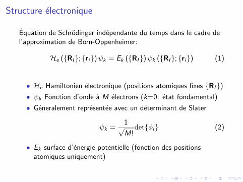
Structure electronique
Equation de Schrodinger independante du temps dans le cadre del’approximation de Born-Oppenheimer:
He ({RI}; {ri})ψk = Ek ({RI})ψk ({RI}; {ri}) (1)
• He Hamiltonien electronique (positions atomiques fixes {RI})• ψk Fonction d’onde a M electrons (k=0: etat fondamental)
• Generalement representee avec un determinant de Slater
ψk =1√M!
det{φi} (2)
• Ek surface d’energie potentielle (fonction des positionsatomiques uniquement)
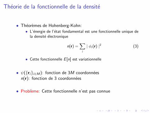
Theorie de la fonctionnelle de la densite
• Theoremes de Hohenberg-Kohn:
• L’energie de l’etat fondamental est une fonctionnelle unique dela densite electronique
n(r) =∑
i
| φi (r) |2 (3)
• Cette fonctionnelle E [n] est variationnelle
• ψ({ri}i∈M): fonction de 3M coordonneesn(r): fonction de 3 coordonnees
• Probleme: Cette fonctionnelle n’est pas connue

Methode de Kohn-Sham
Definition d’un systeme de particules non-interagissantes subissantun potentiel local tel que la densite de ce systeme est la meme quecelle du systeme reel
EKS [{φi}] = Ekin[{φi}] + Eext [n] + EH [n] + Exc [n] (4)
4 termes
• Energie cinetique
Ekin[{φi}] =∑
i
〈φi | −1
2∇2 | φi 〉 (5)
Ne pas confondre avec l’energie cinetique des atomes (DM)
Methode de Kohn-Sham
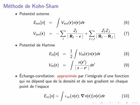
• Potentiel externe
Eext [n] =
∫Vext(r)n(r)dr (6)
Vext(r) = −∑
I
ZI
| RI − r |+
∑I<J
ZIZJ
| RI − RJ |(7)
• Potentiel de Hartree
EH [n] =1
2
∫VH(r)n(r)dr (8)
VH(r) =
∫n(r′)
| r − r′ |dr′ (9)
• Echange-correlation: approximee par l’integrale d’une fonctionqui ne depend que de la densite et de son gradient en chaquepoint de l’espace
Exc [n] =
∫εxc(n(r); ∇n(r))n(r)dr (10)

Pseudopotentiels
Les electrons de cœur ne participent pas aux reactions chimiques→ remplaces par un potentiel effectif
Implications:
• Reduction du nombre d’electrons → acceleration des calculs
• Inclusion partielle des effets relativistes dans ces potentielseffectifs
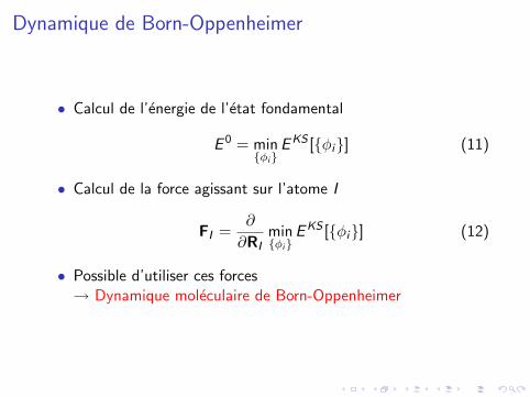
Dynamique de Born-Oppenheimer
• Calcul de l’energie de l’etat fondamental
E 0 = min{φi}
EKS [{φi}] (11)
• Calcul de la force agissant sur l’atome I
FI =∂
∂RImin{φi}
EKS [{φi}] (12)
• Possible d’utiliser ces forces→ Dynamique moleculaire de Born-Oppenheimer
Plan
Theorie de la fonctionnelle de la densite
Methode de Car-Parrinello
Comparaison BO-CP
Exemples
Conclusion - perspectives

Dynamique de Car-Parrinello
• Etat de l’art au debut des annees 80:Calcul auto-coherent de l’etat fondamental; diagonalisation achaque etape de l’Hamiltonien de Kohn-Sham→ impossible a utiliser au cours d’une DM (trop couteux)
• Idee de Car et Parrinello: eviter cette etape
1. Calcul de l’etat fondamental au debut de la dynamique2. Propagation de la fonction d’onde a l’aide d’une equation du
mouvement ensuite

Equations du mouvement
Propagation simultanee des positions et de la fonction d’onde
mI RI = − ∂
∂RI〈ψ0 | He | ψ0〉
µφi = − ∂
∂φ∗i〈ψ0 | He | ψ0〉+
∑j
Λijφj
→ Introduction d’une ”masse electronique fictive” µ

Integration: algorithme Verlet-vitesse˙RI (t + δt) = RI (t) +
δt
2MIFI (t) (13)
RI (t + δt) = RI (t) + δt ˙RI (t + δt) (14)
˙ci (t + δt) = ci (t) +δt
2µfi (t) (15)
c ′i (t + δt) = ci (t) + δt ˙ci (t + δt) (16)
ci (t + δt) = c ′i (t + δt) +∑
j
Xijcj(t) (17)
calcul de FI (t + δt) (18)
calcul de fi (t + δt) (19)
RI (t + δt) = ˙RI (t + δt) +δt
2MIFI (t + δt) (20)
c ′i (t + δt) = ˙ci (t + δt) +δt
2µfi (t + δt) (21)
ci (t + δt) = c ′i (t + δt) +∑
j
Yijcj(t + δt)
(22)

Integration: algorithme Verlet-vitesse˙RI (t + δt) = RI (t) +
δt
2MIFI (t) (13)
RI (t + δt) = RI (t) + δt ˙RI (t + δt) (14)
˙ci (t + δt) = ci (t) +δt
2µfi (t) (15)
c ′i (t + δt) = ci (t) + δt ˙ci (t + δt) (16)
ci (t + δt) = c ′i (t + δt) +∑
j
Xijcj(t) (17)
calcul de FI (t + δt) (18)
calcul de fi (t + δt) (19)
RI (t + δt) = ˙RI (t + δt) +δt
2MIFI (t + δt) (20)
c ′i (t + δt) = ˙ci (t + δt) +δt
2µfi (t + δt) (21)
ci (t + δt) = c ′i (t + δt) +∑
j
Yijcj(t + δt) (22)

La masse electronique fictive
• µ est un parametre non-physique controlant le pas de tempsde la dynamique “classique” suivie par les electrons
• Il faut prendre une valeur optimale permettantI une separation adiabatique entre les deplacements reels des
noyaux et les deplacements artificiels des electronsI un pas de temps d’integration ∆t le plus grand possible
• Valeurs typiques: µ ≈ 300− 1000 ua, ∆t ≈3–10 a.u. =0.07–0.24 fs

Plan
Theorie de la fonctionnelle de la densite
Methode de Car-Parrinello
Comparaison BO-CP
Exemples
Conclusion - perspectives

Comparaison BO-CP pour 32 molecules d’eau: parametres
T=350 K; ρ=0.905 g.cm−3
Simulation Pas de temps Convergence µ(ua) (ua) (ua)
CP 3 – 300
CP 4 – 500
CP 5 – 700
BO 20 10−4 –
BO 20 10−5 –
BO 20 10−6 –
BO 20 10−7 –
40 ua ≈ 1 fs
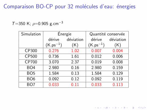
Comparaison BO-CP pour 32 molecules d’eau: energies
T=350 K; ρ=0.905 g.cm−3
Simulation Energie Quantite conserveederive deviation derive deviation
(K.ps−1) (K) (K.ps−1) (K)
CP300 0.276 1.02 0.007 0.004
CP500 0.736 1.61 0.012 0.006
CP700 3.070 2.37 0.019 0.008
BO4 2.980 0.16 2.980 0.159
BO5 1.584 0.13 1.584 0.129
BO6 0.092 0.12 0.092 0.119
BO7 0.033 0.11 0.033 0.113

Comparaison BO-CP
BO MD CP MDToujours sur la surface de BO, Toujours legerementplus “juste” au-dessus de la surface de BO
δt ≈ echelle de temps des atomes δt < echelle de temps des atomes
Diagonalisation ou minimisation Orthogonalisation,couteuse a chaque pas de temps pas de temps moins couteux
Critere de convergence conservatif Stablepour avoir une dynamique stable
Besoin de choisir µ

Plan
Theorie de la fonctionnelle de la densite
Methode de Car-Parrinello
Comparaison BO-CP
Exemples
Conclusion - perspectives

Exemple 1: mecanisme de transfert de proton
Owing to quantum effects, the actual defect structure is bestdescribed as a fluxional defect5. Applying the proton-hole conceptto the OH2 case, one would expect the occurrence of tricoordinateOH2(H2O)3 (in which the hydroxide oxygen accepts three hydro-gen bonds) and H3O2
2 (that is [HO· · ·H· · ·OH]2) complexes,analogous to H3O
!(H2O)3 and H5O!2 ; respectively. Moreover,
structural diffusion would be driven by similar second-solvation-shell fluctuations. Interpretations of Raman and infrared spectra ofconcentrated basic solutions have been guided by the proton-holepicture, a fact that has led to controversies about the structure and
dynamics of hydrated hydroxide14–17. Prompted by this controversy,we undertook an extensive ab initio path integral19,20 study of ahydroxide ion in bulk water at room temperature (see Fig. 2 fordetails).
For each configuration generated in the simulation, the OH2
charge defect, designated (O*H 0)2, is located in the hydrogen-bond(H-bond) network by identifying the oxygen with a single hydro-gen. Next, for each H-bond, a displacement coordinate, ~d"ROaH 2RObH; is defined, where ROa
H and RObH are the distances
between the shared proton and the two oxygens. A small value of dindicates a propensity for proton transfer. Finally, a transfer co-ordinate, d, is defined in each configuration by selecting the H-bondwith the smallest d. This H-bond, designated O*· · ·H*O, is con-sidered to be the ‘most active’ or most likely to experience protontransfer5. Invariably, it is found that one of the oxygens in thisH-bond corresponds to the defect, O*.
In order to identify the role played by various solvation com-plexes of OH2, configurations with large and small jdj are selected.Figure 2a shows that, at large jdj, O* accepts, on average, four H-bonds from neighbouring waters. Representative configurations
Figure 1 Schematic illustration of proton and hydroxide ion transport in water at roomtemperature. Panels a–c show the transport mechanisms of H3O
!, and panels d–f thetransport mechanisms of OH2. Red and grey spheres are oxygen and hydrogen atoms,
respectively, and yellow spheres are the H3O! and OH2 defect oxygens. Dashed green
lines denote hydrogen bonds. These simplified sketches are idealized renderings of the
classical limit of the ‘real’ processes shown in Fig. 3 and Fig. 1 of ref. 5. H3O!
mechanism: In a, the H3O! is shown in a threefold-coordinated, H3O
!(H2O)3, state, and a
complete coordination shell is shown for one of the first-solvation-shell waters. Thermal
fluctuations cause an H-bond breaking between a first and second solvation-shell water of
H3O! to occur (b), leaving the first-solvation-shell water with a threefold coordination
pattern, followed by a shrinking of the first-shell O*O distance and a migration of the
proton to the centre of the bond, forming an intermediate H5O2! complex. Complete
transfer of the proton (c), yields a properly solvated H3O! at a new site in the H-bond
network. The ‘gate closes’ (no further proton transfer events are possible until another
H-bond breaking event occurs) if the newly formed water acquires a fourth H-bond (shown
as the water released by the H-bond breaking event in b, although it could be any nearbysolvent water). OH2 mechanism: In d, the OH2 is shown in a fourfold-coordinated,
OH2(H2O)4, state, and a complete coordinate shell is shown for one of the first-solvation-
shell waters. A neighbouring solvent is shown above the OH2 hydrogen. Thermal
fluctuations cause a first-solvation-shell H-bond breaking event (b), leaving the OH2 in a
threefold OH2(H2O)3 state, followed by a shrinking of a first-shell O*O distance and the
formation of a weak H-bond between the OH2 hydrogen and a neighbouring solvent water
(see, also, Fig. 3b–d). Complete transfer of the proton (f) causes the OH2(H2O)3 to migrateto a new site in the H-bond network. The ‘gate closes’ if the newly formed hydroxide
acquires a fourth H-bond (shown as the water released in b, although it could be anynearby solvent water), to complete the OH2(H2O)4 structure.
Figure 2 Radial distribution functions and coordination numbers during proton transfer.Shown are radial distribution functions, g (r ), and, on the same scale, running
coordination numbers, N (r ), with respect to the hydroxide ion and a first-solvation-shell
water at different stages in the proton transfer process. a, Radial distribution functions,g O*O (solid blue) and g O*H (solid red) and coordination numbers, N O*O (dashed blue) and
N O*H (dashed red), with respect to the OH2, O*, for values of the proton transfer
coordinate jdj" RO*H* 2 R !OH* . 0:5 "A: Here, H* denotes the shared proton, and Odenotes the oxygen of a water molecule that donates the ‘most active’ H-bond to O*, that
is, O*· · ·H*O. b, As a except for jdj , 0.1 A. c, Two-dimensional generalization of ahydrogen-oxygen radial distribution function g H 0O(r,jdj) with respect to the OH2hydrogen, H 0 , as a function of r and jdj. d, Radial distribution functions and coordinationnumbers with respect to O for jdj , 0.1 A. The colour and line types are the same as in a.Coordination numbers from b are superimposed with red (O*H) and blue (O*O) circles. Thesimulations were performed using CPMD Version 3.0 (J. Hutter et al., Max-Planck-Institut
fur Festkorperforschung and IBM Zurich Research Laboratory 1995–1996)21 at ambient
conditions using 31 H2O with one OH2 anion in a periodic cubic box of side length
9.8692 A, employing the BLYP functional, Troullier-Martins type pseudopotentials, and a
G-point plane wave expansion of the valence orbitals up to 70 Ry. This particular scheme
has been shown to yield a good description of dynamical processes in aqueous
systems5,6,30,32. The path integral was discretized using P " 8 Trotter replicas following
the methodology of ref. 20. After careful equilibration, quantum and classical nuclear
trajectories consisting of 322,000 and 346,000 configurations, with time steps of 5.0 a.u.
and 7.0 a.u., respectively, were generated via the Car-Parrinello algorithm22.
letters to nature
NATURE | VOL 417 | 27 JUNE 2002 | www.nature.com/nature926 © 2002 Nature Publishing Group
a) H3O+ coordonne par 3 molecules d’eau.a) Rupture d’une liaison H entre une moleculea) de la 1ere sphere de solvatation et une de la 2de.
Owing to quantum effects, the actual defect structure is bestdescribed as a fluxional defect5. Applying the proton-hole conceptto the OH2 case, one would expect the occurrence of tricoordinateOH2(H2O)3 (in which the hydroxide oxygen accepts three hydro-gen bonds) and H3O2
2 (that is [HO· · ·H· · ·OH]2) complexes,analogous to H3O
!(H2O)3 and H5O!2 ; respectively. Moreover,
structural diffusion would be driven by similar second-solvation-shell fluctuations. Interpretations of Raman and infrared spectra ofconcentrated basic solutions have been guided by the proton-holepicture, a fact that has led to controversies about the structure and
dynamics of hydrated hydroxide14–17. Prompted by this controversy,we undertook an extensive ab initio path integral19,20 study of ahydroxide ion in bulk water at room temperature (see Fig. 2 fordetails).
For each configuration generated in the simulation, the OH2
charge defect, designated (O*H 0)2, is located in the hydrogen-bond(H-bond) network by identifying the oxygen with a single hydro-gen. Next, for each H-bond, a displacement coordinate, ~d"ROaH 2RObH; is defined, where ROa
H and RObH are the distances
between the shared proton and the two oxygens. A small value of dindicates a propensity for proton transfer. Finally, a transfer co-ordinate, d, is defined in each configuration by selecting the H-bondwith the smallest d. This H-bond, designated O*· · ·H*O, is con-sidered to be the ‘most active’ or most likely to experience protontransfer5. Invariably, it is found that one of the oxygens in thisH-bond corresponds to the defect, O*.
In order to identify the role played by various solvation com-plexes of OH2, configurations with large and small jdj are selected.Figure 2a shows that, at large jdj, O* accepts, on average, four H-bonds from neighbouring waters. Representative configurations
Figure 1 Schematic illustration of proton and hydroxide ion transport in water at roomtemperature. Panels a–c show the transport mechanisms of H3O
!, and panels d–f thetransport mechanisms of OH2. Red and grey spheres are oxygen and hydrogen atoms,
respectively, and yellow spheres are the H3O! and OH2 defect oxygens. Dashed green
lines denote hydrogen bonds. These simplified sketches are idealized renderings of the
classical limit of the ‘real’ processes shown in Fig. 3 and Fig. 1 of ref. 5. H3O!
mechanism: In a, the H3O! is shown in a threefold-coordinated, H3O
!(H2O)3, state, and a
complete coordination shell is shown for one of the first-solvation-shell waters. Thermal
fluctuations cause an H-bond breaking between a first and second solvation-shell water of
H3O! to occur (b), leaving the first-solvation-shell water with a threefold coordination
pattern, followed by a shrinking of the first-shell O*O distance and a migration of the
proton to the centre of the bond, forming an intermediate H5O2! complex. Complete
transfer of the proton (c), yields a properly solvated H3O! at a new site in the H-bond
network. The ‘gate closes’ (no further proton transfer events are possible until another
H-bond breaking event occurs) if the newly formed water acquires a fourth H-bond (shown
as the water released by the H-bond breaking event in b, although it could be any nearbysolvent water). OH2 mechanism: In d, the OH2 is shown in a fourfold-coordinated,
OH2(H2O)4, state, and a complete coordinate shell is shown for one of the first-solvation-
shell waters. A neighbouring solvent is shown above the OH2 hydrogen. Thermal
fluctuations cause a first-solvation-shell H-bond breaking event (b), leaving the OH2 in a
threefold OH2(H2O)3 state, followed by a shrinking of a first-shell O*O distance and the
formation of a weak H-bond between the OH2 hydrogen and a neighbouring solvent water
(see, also, Fig. 3b–d). Complete transfer of the proton (f) causes the OH2(H2O)3 to migrateto a new site in the H-bond network. The ‘gate closes’ if the newly formed hydroxide
acquires a fourth H-bond (shown as the water released in b, although it could be anynearby solvent water), to complete the OH2(H2O)4 structure.
Figure 2 Radial distribution functions and coordination numbers during proton transfer.Shown are radial distribution functions, g (r ), and, on the same scale, running
coordination numbers, N (r ), with respect to the hydroxide ion and a first-solvation-shell
water at different stages in the proton transfer process. a, Radial distribution functions,g O*O (solid blue) and g O*H (solid red) and coordination numbers, N O*O (dashed blue) and
N O*H (dashed red), with respect to the OH2, O*, for values of the proton transfer
coordinate jdj" RO*H* 2 R !OH* . 0:5 "A: Here, H* denotes the shared proton, and Odenotes the oxygen of a water molecule that donates the ‘most active’ H-bond to O*, that
is, O*· · ·H*O. b, As a except for jdj , 0.1 A. c, Two-dimensional generalization of ahydrogen-oxygen radial distribution function g H 0O(r,jdj) with respect to the OH2hydrogen, H 0 , as a function of r and jdj. d, Radial distribution functions and coordinationnumbers with respect to O for jdj , 0.1 A. The colour and line types are the same as in a.Coordination numbers from b are superimposed with red (O*H) and blue (O*O) circles. Thesimulations were performed using CPMD Version 3.0 (J. Hutter et al., Max-Planck-Institut
fur Festkorperforschung and IBM Zurich Research Laboratory 1995–1996)21 at ambient
conditions using 31 H2O with one OH2 anion in a periodic cubic box of side length
9.8692 A, employing the BLYP functional, Troullier-Martins type pseudopotentials, and a
G-point plane wave expansion of the valence orbitals up to 70 Ry. This particular scheme
has been shown to yield a good description of dynamical processes in aqueous
systems5,6,30,32. The path integral was discretized using P " 8 Trotter replicas following
the methodology of ref. 20. After careful equilibration, quantum and classical nuclear
trajectories consisting of 322,000 and 346,000 configurations, with time steps of 5.0 a.u.
and 7.0 a.u., respectively, were generated via the Car-Parrinello algorithm22.
letters to nature
NATURE | VOL 417 | 27 JUNE 2002 | www.nature.com/nature926 © 2002 Nature Publishing Group
b) Une des molecules d’eau de la 1ere sphere estb) coordonnee 3 fois (au lieu de 4).b) Migration du proton au milieu de la liaison,b) avec formation d’un complexe H5O+
2 intermediaire.
Owing to quantum effects, the actual defect structure is bestdescribed as a fluxional defect5. Applying the proton-hole conceptto the OH2 case, one would expect the occurrence of tricoordinateOH2(H2O)3 (in which the hydroxide oxygen accepts three hydro-gen bonds) and H3O2
2 (that is [HO· · ·H· · ·OH]2) complexes,analogous to H3O
!(H2O)3 and H5O!2 ; respectively. Moreover,
structural diffusion would be driven by similar second-solvation-shell fluctuations. Interpretations of Raman and infrared spectra ofconcentrated basic solutions have been guided by the proton-holepicture, a fact that has led to controversies about the structure and
dynamics of hydrated hydroxide14–17. Prompted by this controversy,we undertook an extensive ab initio path integral19,20 study of ahydroxide ion in bulk water at room temperature (see Fig. 2 fordetails).
For each configuration generated in the simulation, the OH2
charge defect, designated (O*H 0)2, is located in the hydrogen-bond(H-bond) network by identifying the oxygen with a single hydro-gen. Next, for each H-bond, a displacement coordinate, ~d"ROaH 2RObH; is defined, where ROa
H and RObH are the distances
between the shared proton and the two oxygens. A small value of dindicates a propensity for proton transfer. Finally, a transfer co-ordinate, d, is defined in each configuration by selecting the H-bondwith the smallest d. This H-bond, designated O*· · ·H*O, is con-sidered to be the ‘most active’ or most likely to experience protontransfer5. Invariably, it is found that one of the oxygens in thisH-bond corresponds to the defect, O*.
In order to identify the role played by various solvation com-plexes of OH2, configurations with large and small jdj are selected.Figure 2a shows that, at large jdj, O* accepts, on average, four H-bonds from neighbouring waters. Representative configurations
Figure 1 Schematic illustration of proton and hydroxide ion transport in water at roomtemperature. Panels a–c show the transport mechanisms of H3O
!, and panels d–f thetransport mechanisms of OH2. Red and grey spheres are oxygen and hydrogen atoms,
respectively, and yellow spheres are the H3O! and OH2 defect oxygens. Dashed green
lines denote hydrogen bonds. These simplified sketches are idealized renderings of the
classical limit of the ‘real’ processes shown in Fig. 3 and Fig. 1 of ref. 5. H3O!
mechanism: In a, the H3O! is shown in a threefold-coordinated, H3O
!(H2O)3, state, and a
complete coordination shell is shown for one of the first-solvation-shell waters. Thermal
fluctuations cause an H-bond breaking between a first and second solvation-shell water of
H3O! to occur (b), leaving the first-solvation-shell water with a threefold coordination
pattern, followed by a shrinking of the first-shell O*O distance and a migration of the
proton to the centre of the bond, forming an intermediate H5O2! complex. Complete
transfer of the proton (c), yields a properly solvated H3O! at a new site in the H-bond
network. The ‘gate closes’ (no further proton transfer events are possible until another
H-bond breaking event occurs) if the newly formed water acquires a fourth H-bond (shown
as the water released by the H-bond breaking event in b, although it could be any nearbysolvent water). OH2 mechanism: In d, the OH2 is shown in a fourfold-coordinated,
OH2(H2O)4, state, and a complete coordinate shell is shown for one of the first-solvation-
shell waters. A neighbouring solvent is shown above the OH2 hydrogen. Thermal
fluctuations cause a first-solvation-shell H-bond breaking event (b), leaving the OH2 in a
threefold OH2(H2O)3 state, followed by a shrinking of a first-shell O*O distance and the
formation of a weak H-bond between the OH2 hydrogen and a neighbouring solvent water
(see, also, Fig. 3b–d). Complete transfer of the proton (f) causes the OH2(H2O)3 to migrateto a new site in the H-bond network. The ‘gate closes’ if the newly formed hydroxide
acquires a fourth H-bond (shown as the water released in b, although it could be anynearby solvent water), to complete the OH2(H2O)4 structure.
Figure 2 Radial distribution functions and coordination numbers during proton transfer.Shown are radial distribution functions, g (r ), and, on the same scale, running
coordination numbers, N (r ), with respect to the hydroxide ion and a first-solvation-shell
water at different stages in the proton transfer process. a, Radial distribution functions,g O*O (solid blue) and g O*H (solid red) and coordination numbers, N O*O (dashed blue) and
N O*H (dashed red), with respect to the OH2, O*, for values of the proton transfer
coordinate jdj" RO*H* 2 R !OH* . 0:5 "A: Here, H* denotes the shared proton, and Odenotes the oxygen of a water molecule that donates the ‘most active’ H-bond to O*, that
is, O*· · ·H*O. b, As a except for jdj , 0.1 A. c, Two-dimensional generalization of ahydrogen-oxygen radial distribution function g H 0O(r,jdj) with respect to the OH2hydrogen, H 0 , as a function of r and jdj. d, Radial distribution functions and coordinationnumbers with respect to O for jdj , 0.1 A. The colour and line types are the same as in a.Coordination numbers from b are superimposed with red (O*H) and blue (O*O) circles. Thesimulations were performed using CPMD Version 3.0 (J. Hutter et al., Max-Planck-Institut
fur Festkorperforschung and IBM Zurich Research Laboratory 1995–1996)21 at ambient
conditions using 31 H2O with one OH2 anion in a periodic cubic box of side length
9.8692 A, employing the BLYP functional, Troullier-Martins type pseudopotentials, and a
G-point plane wave expansion of the valence orbitals up to 70 Ry. This particular scheme
has been shown to yield a good description of dynamical processes in aqueous
systems5,6,30,32. The path integral was discretized using P " 8 Trotter replicas following
the methodology of ref. 20. After careful equilibration, quantum and classical nuclear
trajectories consisting of 322,000 and 346,000 configurations, with time steps of 5.0 a.u.
and 7.0 a.u., respectively, were generated via the Car-Parrinello algorithm22.
letters to nature
NATURE | VOL 417 | 27 JUNE 2002 | www.nature.com/nature926 © 2002 Nature Publishing Group
c) Transfert complet du proton.
D. Marx, M.E. Tuckerman, J. Hutter & M. Parrinello, Nature 397, 601 (1999)

Exemple 2: constante d’auto-ionisation Ke de l’eau
!"#$#!%&$'(%'! )*$ # !*+%#!% '*+ ,#'$- %"& )$&& &+&$./!0$1& '+ 2'.3 4 (%'55 ("*6( # 7+'%& ,*('%'1& (5*,&38"& !5*(&(% %* # %$#+('%'*+ (%#%& '( %"& !*+7.0$#9%'*+ $&(,*+(':5& )*$ %"& ;'+';0; '+ %"& ;&#+)*$!& #% !< ! =!> ?2'.3 >@- # (*51&+% (&,#$#%&A '*+,#'$3
8"'( !*;,5&B- 6'%" ?#5;*(%@ 1#+'("'+. ;&#+)*$!&- "#( # A'(%'+!% #+A '+%&$&(%'+. (%$0!%0$&3 C(+#,("*% (#;,5&A )$*; %"& !*+(%$#'+&A DE $0+ #%!< " =!> '( ("*6+ '+ 2'.3 F3 8"& (%$0!%0$& &B%&+A(*1&$ %6* $'+. ,&+%#;&$( *) "/A$*.&+ :*+A( !*+9('(%'+. *) )*0$ 6#%&$ ;*5&!05&( &#!" ,50( %"& !*+9(%$#'+&A "/A$*B/5 .$*0, #( %"& !&+%$#5 ("#$&A 7)%"!*;,*+&+%3 8"& )$#;&6*$G *) %"& +'+& *B/.&+#%*;( '( #,,$*B';#%&5/ ,5#+#$3 8"& H< :*+A *)%"& "/A$*B/5 '( ,&$,&+A'!05#$ %* %"'( ,5#+&3 8"&&B!&(( ,$*%*+ '( $&('A'+. *+ *+& *) %"& %6* ,&+9%#;&$'! 6'+.( #+A '( #((*!'#%&A 6'%" %"& %6* *0%&$<IH ;*5&!05&( +*% A'$&!%5/ "/A$*.&+ :*+A&A %*%"& <H#3 8"'( A';&$ *) 6#%&$ ;*5&!05&( "*5A'+.
%"& &B!&(( ,$*%*+ !#+ :& 1'&6&A #( !*+(%'%0%'+. #+<JH
$I '*+ )#!'+. %"& <H#3 8"& <JH
$I (,&!'&(-
(*;&%';&( !#55&A K0+A&59'*+- '( # )#;'5'#$ (%$0!9%0$#5 ;*%'1& *) <$ (*51#%'*+ ?L&)(3 MN-=O-=IP@3 8"&(%$0!%0$& '+ 2'.3 F Q0#5'7&( #( # (*51&+% (&,#$#%&A'*+ ,#'$ :&!#0(& *) %"& %6* <IH ;*5&!05&( *) %"&,&+%#;&$ 6"'!" #$& '+ %"& !*$$&!% ,*('%'*+ #+A*$'&+%#%'*+ %* #!% #( (0'%#:5& 5'.#+A( %* :*%" %"&!#%'*+ #+A %"& #+'*+3
R';'5#$ ,&+%#;&$'! (*51&+% (&,#$#%&A '*+ ,#'$("#1& :&&+ *:(&$1&A :/ A'S$#!%'*+ &B,&$';&+%( '+#Q0&*0( <T5 6'%" "#5'A& '*+( $&,5#!'+. %"& <H#
MI4P3 20$%"&$ (0,,*$% )*$ %"& (%#:'5'%/ *) %"&(&(%$0!%0$&( !*;&( )$*; !*;,0%#%'*+#5 (%0A'&( *)#0%*A'((*!'#%'*+ '+ (;#55 !50(%&$( MIFP3 H) ,#$%'!095#$ $&5&1#+!& #$& %"& !#5!05#%'*+( *) A',*5& ;*9;&+%( MIUP3 T*;,#$'+. $&#!%#+% !50(%&$( #+A %"&V6'%%&$9'*+'! ,$*A0!%(- '% 6#( )*0+A %"#% %"&!"#$.& (&,#$#%'*+ '+ )#!% $&A0!&( %"& A',*5& ;*9;&+%3 8"'( '( # (%$'G'+. '550(%$#%'*+ *) %"& &W!'&+!/*) (!$&&+'+. :/ *+& *$ %6* '+%&$;&A'#%& #$$#/( *)6#%&$ ;*5&!05&( 6'%" ;#%!"'+. "/A$*.&+ :*+A'+.38"'( &S&!% '( ;*(% 5'G&5/ +*% $&(%$'!%&A %* !50(%&$(#+A !#+ %"&$&)*$& "&5, &B,5#'+ %"& $&5#%'1& &#(&6'%" 6"'!" %"& !*+%#!% '*+ ,#'$ '+ (*50%'*+ !#+ :&A'((*51&A3
C( !#+ :& (&&+ '+ 2'.3 F- %"& A*0:5& ,&+%#;&$'!!*;,5&B '( $#%"&$ 5#$.& (%$&%!"'+. )$*; *+& &+A *)*0$ !0:'! DE !&55 %* %"& *%"&$3 X+ )#!%- ('+!& %"&DE (/(%&; '( ,&$'*A'!- %"& <IH A';&$ :'+A'+.%"& <$ '*+ '( !*++&!%&A :/ "/A$*.&+ :*+A( %* %"&';#.& *) %"& &Q0'1#5&+% A';&$ *+ %"& *,,*('%&,&+%#;&$3 8"'( ';;&A'#%&5/ $#'(&( (&$'*0( Q0&(9%'*+( #:*0% :*0+A#$/ &S&!%( '+ *0$ (;#55 (/(%&;3X+ ,#$%'!05#$- '% !#++*% :& &B!50A&A %"#% %"&#,,#$&+% !*;;&+(0$#:'5'%/ 6'%" %"& ,&$'*A'!:*0+A#$/ !*+A'%'*+( '( # (0:(%#+%'#5 (%#:'5'V'+.)#!%*$ )*$ %"& (*51&+% (&,#$#%&A '*+ ,#'$ '+ 2'.3 F320$%"&$;*$&- %"& !*0,5'+. :&%6&&+ &+A A';&$( 1'#%"&'$ ,&$'*A'! ';#.&( *,&+( 0, # !*+1&+'&+%,#%"6#/ *) #5'.+&A "/A$*.&+ :*+A( #5*+. 6"'!"%"& <$ !#+ :& ("0%%5&A %* %"& <H# '+ %"& #AY#!&+%!&553 X) +*% !"&!G&A :/ # .&+&$'! !*+(%$#'+% ,$*9%&!%'+. %"& "/A$*B/5 .$*0,- %"'( 6*05A ('.+'7!#+%5/&+"#+!& %"& G'+&%'! '+(%#:'5'%/3 R0!" # (&$'&( *),$*%*+ "*,( 6$#,,'+. #$*0+A %"& DE !&55 6#(#!%0#55/ *:(&$1&A '+ %"& :*+A !*+(%$#'+% (';05#9%'*+ *) L&)(3 M=J-=4P3
2'.3 F3 X+(%#+%#+&*0( ;*5&!05#$ !*+7.0$#%'*+ (#;,5&A )$*; #!*+(%$#'+&A #: '+'%'* DE $0+ #% !< " =!> ("*6'+. # (*51&+%(&,#$#%&A '*+ ,#'$ ?*B/.&+( Z .$&/- ,$*%*+( Z :5#!G@3 8"&A*0:5& ,&+%#;&$'! !*;,5&B- 6'%" %"& "/A$*B/5 '*+ #% %"& !&+%$&#+A %"& ,$*%*+ #:(%$#!%&A )$*; '% *+ *+& *) %"& 6'+.(- '("'."5'."%&A :/ #+ &+"#+!&A (%'!G #+A :#55 $&,$&(&+%#%'*+3 H+5/%"& "/A$*.&+ :*+A( *) %"& ,&+%#;&$'! !*;,5&B ?%"'!G A#("&A5'+&(@ #$& '+A'!#%&A3
=[U !" #$%&' ( )*+,&-./ 0*12&-2 345 637778 9:;<947
Calculee avec diverses coordonnees dereaction:
• Nombre de coordination du proton
• Nombre de coordination de l’oxygene
• Longueur de la liaison OH
Toutes les methodes donnent pKe=13±1
M Sprik, Chem. Phys. 258, 139 (2000)

Exemple 3: constante d’acidite Ka de l’histidine
A snapshot of a typical configuration and a schematic repre-sentation of the histidine dissociation reaction are shown inFigures 1a and 1b, respectively. For the reference reaction, waterautodissociation, we used a system containing 32 water mol-ecules in a cubic box of 9.86 ! 9.86 ! 9.86 Å with periodicboundary conditions. The size of the systems considered issufficient to provide the complete first and second solvationshells of the solute (either a histidine or a water molecule) pluspart of the third shell. This fact makes comparison between thetwo systems fully meaningful. All simulations were performedwith the program CPMD.11 The gradient-corrected HCTH12,13functional was adopted. In addition to providing good structuraldescription of aqueous systems, this functional yields improvedenergetics compared to the popular BLYP14,15 functional,specifically for hydrogen abstraction reactions in the gas phase.12The core electrons were accounted for in our simulations bynonlocal norm-conserving pseudopotentials of the Troullier-Martins16 type. For the heavy atoms these have been transformedto a fully nonlocal form using the scheme of Kleinman andBylander.17 The valence electronic wave functions were ex-panded in a plane wave basis set with an energy cutoff of 70Ry. Hydrogen nuclei were treated as classical particles with themass of the deuterium isotope. Thus, the nuclear quantum effectswere not included in our simulation. Nevertheless, quantumeffects might be significantly manifested for this reaction. Thedifference between the zero point energies (!ZPE) associatedwith imidazolium ion deprotonation and the reference waterautodissociation reaction can serve as an estimate for themagnitude of these effects and their influence on the calculatedfree energies. In this respect, the advantage of calculating relativepKa values becomes apparent: By selecting a reference reaction,for which the ZPE contribution is expected to be comparable,we can minimize the influence of the nuclear quantum effectson the results. In our case, the calculated !!ZPE (Table 1 ofthe Supporting Information) of -0.46 kcal mol-1 correspondsto a shift in the estimated pKa of-0.34 units and is considerably
below the inherent accuracy of the DFT functional. To fullyaccount for nuclear quantum effects (including tunneling) onehas to carry out expensive path integral simulations, which arebeyond the scope of the current work. A fictitious mass of 800au was ascribed to the electronic degrees of freedom consistentwith the recommended "1/5 of the mass of deuterium iso-tope.18,19 This choice allowed the equations of motion for theatomic nuclei to be propagated with a time step of 0.15 fs. Theadiabatic separation of the nuclear and electronic subsystemsis fully preserved along all AIMD trajectories. The simulationswere performed in the NVT ensemble, and the temperature wasmaintained at "300 K by the use of a Nose-Hoover chain ofthermostats20,21 with a chain length of four and a target frequencyof 500 cm-1. This set of parameters enabled us to maintainadiabatic conditions for the electrons over the full length of thetrajectories.
3. Results and Discussion3.1. Potentials of Mean Force. Weak acid dissociation is a
rare event on the time scale of ab initio molecular dynamicsand thus not accessible through direct simulations. Constrainedmolecular dynamics can circumvent this difficulty and enforcedissociation, through the use of a control parameter !, typicallychosen to resemble the respective reaction coordinate, whosevalues are held constant and then varied in increments through-out the simulation.22-24 When the underlying potential energysurface is inherently complex in multiple dimensions, as is oftenthe case for condensed phase reactions, the use of simplegeometric constraints can be a rather poor approximation to thetrue reaction coordinate and can lead to problems, especiallyin attempts to locate transition states.23 Nevertheless, geometricconstraints that distinguish unambiguously between reactant andproduct states can still be utilized to determine free energydifferences.23,24 This is due to the fact that the Helmholtz freeenergy is a function of state and, thus, independent of the exactreversible path used to connect the initial and final states. Bothsimple linear5,6 and collective7 (e.g., coordination) constraintshave been applied to the problem of water autodissociation. Theadvantage of the latter lies in the ability to control thecoordination of a species (protonation state in the case ofhydrogen coordination) without the need to specify distancesto particular hydrogen atoms. This, in turn, prevents ionrecombination that would normally occur with linear constraintsat the end of the PMF due to proton transfer. In our presentinvestigation we have relied on linear constraints, primarily fortheir simplicity. In particular, the N*-H distance between oneof the imidazole nitrogens and its neighboring hydrogen (! )|rN* - rH|) was varied between 0.8 and 1.8 Å with an incrementof 0.05 Å. For each constrained configuration we have obtainedtrajectories starting from well-equilibrated unconstrained con-figurations. After reequilibration for 1.0 ps the properties ofinterest were averaged for an additional 10 ps. The constraintwas linearly added to the CP Lagrangian according to the bluemoon ensemble method.22,24 The method corrects for the biasin the statistics for momentum space due to the introduction ofconstraints in coordinate space. Within this method the relativefree energy between states !0 and !1 can be evaluated using theexpressions
where f! is the average force of constraint, kB is the Boltzmannconstant, T is the temperature in Kelvin, and Z and G are weight
Figure 1. (a) Snapshot of a typical configuration from an unconstraineddynamics trajectory. The hydrogen, carbon, oxygen, and nitrogen atomsare color-coded in white, gray, red, and blue; the positions of theWannier function centers (centers of charge of localized molecularorbitals,9 indicative of the bonding pattern, are shown in gold. (b)Schematic representation of the deprotonation reaction.
!F ) -#!0
!1 f!!d!! f!! )
"Z-1/2[" - kBTG]#!!"Z-1/2#!!
(1)
6366 J. Phys. Chem. B, Vol. 110, No. 12, 2006 Ivanov et al.
and correction factors associated with the transformation fromgeneralized to Cartesian coordinates.24 In the case of a distanceconstraint the second equation reduces to a simple ensembleaverage of the Lagrange multiplier !: f"! ) "!#"!.The free energy profiles resulting from the above integration
are plotted in Figure 2. The dissociation of histidine proceedsin several stages.22 In summary, first the polar N*-H bond isextended harmonically; then the bond transformation (conver-sion of the N*-H bond from covalent to hydrogen) takes placefrom " ! 1.2 to 1.35 Å; at 1.4 Å the proton is completelytransferred to the O*, and therefore, the free energy curves leveloff after this point; from about " ! 1.5 Å proton transferattempts from the newly formed hydronium ion becomepossible; these are generally not successful until after thetransition state (at separation " ! 1.6-1.65 Å), when theconstraint force changes its sign.The pKa value for a weak acid in aqueous solution can be
related to the value of the Helmholtz free energy for thehydrogen abstraction reaction. Thus, the dissociation constantcan be represented as follows1,27
where Kc is the equilibrium constant for dissociation (expressedin terms of concentration), C0 is the standard concentration, H(r)is a Heaviside function, w(r) ) !F(r) is the potential of meanforce, and Rc is a distance cutoff used to distinguish betweenthe case of a covalently bonded and a dissociated H atom. Thecontribution in eq 2 from values of r below 0.8 Å is negligibledue to the fact that the w(r) term appears in the exponent anddue to the steep increase in the PMF in that region. The aboveexpression shows that direct estimation of the pKa value fromthe energy difference at the two ends of the PMF can beproblematic for two reasons. First, it ignores an entropiccontribution from the bond-breaking process, leading to amissing volume-dependent term in the expression for Ka.Second, what is available from simulations are relative potentialsof mean force, referred to a finite separation between theproducts. Therefore, absolute pKa determination from these datais difficult. However, one may take advantage of the fact thatfrom some distance on, after the transition state, the PMFbecomes rather generic. (Namely, it corresponds to two ions
being separated further and further in solution.) This opens upthe possibility that the determination of relative pKa values maybe less error prone. By taking the ratio of dissociation constantsfor the reaction under consideration and a reference reaction,according to eq 2 we obtain
3.2. pKa and Statistical Accuracy. Potentials of mean forcethat begin at the equilibrium N-H bond length, correspondingto the free energy minimum for the covalent N-H bond mayserve as a reasonable basis for comparison between thetautomeric forms of histidine and a capped analog.22 However,for the purposes of calculating relative pKa values they need tobe extended both in the direction of shortening as well aslengthening of the N-H bond (Figure 2). The length of ourPMF is limited by the onset of proton transfer toward the endof the simulation. For large values of " this process renders alinear constraint ineffective in enforcing the desired reactioncoordinate and prevents further extension of the PMF.We have used a rigorous approach, stemming from statistical
mechanics, to calculate the ratio of equilibrium constants forthe deprotonation of histidine and for a reference reaction (waterautodissociation), which takes into account the aforementionedentropic contribution. By integrating the potentials of mean forceaccording to eq 3 and setting the cutoff radius Rc to 1.35 Å (fordetails, see section 3.3) we obtain a pKa estimate of 6.8. Thisappears to be in good agreement with the experimental valueof 6.1. Closer agreement is not to be expected, given the presentlevel of accuracy of the DFT functionals, the statisticaluncertainty associated with thermodynamic integration, and thefact that contributions from !ZPE and possible quantumtunneling of the proton (see remarks at the end of section 2)are neglected. Since the dissociation constant K is related tothe free energy difference through an exponential relationshipsmall errors in the !F term can lead to relatively large deviationsin Ka. Nevertheless, as we have shown, this approach issufficiently robust to provide useful estimates of pKa and freeenergy differences. It is expected to be applicable to systemsmuch more complicated than the test case of histidine.A few comments are in order regarding the convergence of
the results. The typical length of the constrained trajectories inour study (after equilibration) has reached 10 ps. This amountsto 10 times longer sampling compared to all previous con-strained AIMD studies. During this time the constraint forcesand correspondingly the points of the PMF can be convergedwith very small statistical uncertainties. (Figure 3 depicts therunning average of the calculated constraint force for typicaltrajectories.) While this fact does not completely preclude thepossibility of systematic deviations, which may occur at longertimes, the solvent degrees of freedom are adequately sampledin our simulations (including the fast intramolecular vibrations,rotational motion, librations, and even the more large-scalecollective motions of the water molecules). Most importantly,substantial reorganization of the hydrogen bond network aroundthe solute is seen on this time scale. Hydrogen bond rearrange-ment has been put forth as an important contribution of thesolvent toward stabilizing the products of the dissociation.28 Itshould also be mentioned that AIMD has an inherent advantagein terms of sampling when compared to classical moleculardynamics for reactions involving separation of charge. In thatcase, the instantaneous response of the solvent electronic degrees
Figure 2. Potentials of mean force: (i) for the deprotonation ofL-histidine from the N! position (shown in red) and (ii) for waterautodissociation (shown in green).
Kc-1 ) C0"0$ H(r) e-#w(r)4$r2 dr H(r) ) {1 r < Rc
0 r g Rc(2)
Kd(His)Kd(H2O)
)"0Rc e-#wH2O(r)r2 dr
"0Rc e-#wHis(r)r2 dr(3)
Relative pKa Values from AIMD J. Phys. Chem. B, Vol. 110, No. 12, 2006 6367
Coordonnee de reaction: longueur de la liaison→ pKa=6.8, tres bon accord avec l’experience (6.1)
I. Ivanov, B. Chen, S. Raugei & M.L. Klein, J. Phys. Chem. B 110, 6365 (2006)

Plan
Theorie de la fonctionnelle de la densite
Methode de Car-Parrinello
Comparaison BO-CP
Exemples
Conclusion - perspectives

Codes disponibles
• CPMD
• VASP
• CASTEP
• SIESTA
• CP2K
• QUANTUM-ESPRESSO

Dynamique moleculaire ab initio ?
I Fonctionnelle d’echange-correlation (LDA, GGA: BLYP, PBE,hybrides)
I Remplacement des electrons de coeur par un pseudopotentiel
I Ondes planes: Energie de coupure
I Bases localisees: Choix des bases
I Traitement de la dispersion (Grimme...)
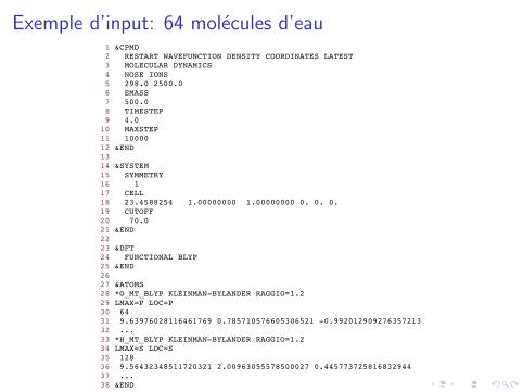
Exemple d’input: 64 molecules d’eau 23/03/10 03:58~/Recherche/Redaction/Presentations/lecture-niigata-mars2010/64mol-example/md-forpdf.in.html
Page 1 sur 1file:///Users/salanne/Recherche/Redaction/Presentations/lecture-niigata-mars2010/64mol-example/md-forpdf.html
1 &CPMD 2 RESTART WAVEFUNCTION DENSITY COORDINATES LATEST 3 MOLECULAR DYNAMICS 4 NOSE IONS 5 298.0 2500.0 6 EMASS 7 500.0 8 TIMESTEP 9 4.010 MAXSTEP11 1000012 &END13 14 &SYSTEM15 SYMMETRY16 117 CELL18 23.4588254 1.00000000 1.00000000 0. 0. 0.19 CUTOFF20 70.021 &END22 23 &DFT24 FUNCTIONAL BLYP25 &END26 27 &ATOMS28 *O_MT_BLYP KLEINMAN-BYLANDER RAGGIO=1.229 LMAX=P LOC=P30 6431 9.63976028116461769 0.785710576605306521 -0.99201290927635721332 ...33 *H_MT_BLYP KLEINMAN-BYLANDER RAGGIO=1.234 LMAX=S LOC=S35 12836 9.56432348511720321 2.00963055578500027 0.44577372581683294437 ...38 &END

Pour aller plus loin...
D. Marx and J. Hutter,Ab Initio Molecular Dynamics: Basic Theory and Advanced Methods
(Cambridge University Press, Cambridge 2009)
ISBN:978–0–521–89863–8