Dynamics of solitons in optical fibres

This article was downloaded by: [University of California Davis]On: 26 October 2014, At: 16:28Publisher: Taylor & FrancisInforma Ltd Registered in England and Wales Registered Number: 1072954 Registeredoffice: Mortimer House, 37-41 Mortimer Street, London W1T 3JH, UK

Journal of Modern OpticsPublication details, including instructions for authors andsubscription information:http://www.tandfonline.com/loi/tmop20

Dynamics of solitons in optical fibresAnjan Biswas a & Alejandro B. Aceves aa Department of Mathematics and Statistics , University of NewMexico , Albuquerque, NM, 87131, USAPublished online: 03 Jul 2009.

To cite this article: Anjan Biswas & Alejandro B. Aceves (2001) Dynamics of solitons in optical fibres,Journal of Modern Optics, 48:7, 1135-1150

To link to this article: http://dx.doi.org/10.1080/09500340108231758

PLEASE SCROLL DOWN FOR ARTICLE

Taylor & Francis makes every effort to ensure the accuracy of all the information (the“Content”) contained in the publications on our platform. However, Taylor & Francis,our agents, and our licensors make no representations or warranties whatsoever as tothe accuracy, completeness, or suitability for any purpose of the Content. Any opinionsand views expressed in this publication are the opinions and views of the authors,and are not the views of or endorsed by Taylor & Francis. The accuracy of the Contentshould not be relied upon and should be independently verified with primary sourcesof information. Taylor and Francis shall not be liable for any losses, actions, claims,proceedings, demands, costs, expenses, damages, and other liabilities whatsoever orhowsoever caused arising directly or indirectly in connection with, in relation to or arisingout of the use of the Content.

This article may be used for research, teaching, and private study purposes. Anysubstantial or systematic reproduction, redistribution, reselling, loan, sub-licensing,systematic supply, or distribution in any form to anyone is expressly forbidden. Terms &Conditions of access and use can be found at http://www.tandfonline.com/page/terms-and-conditions

http://www.tandfonline.com/loi/tmop20

http://dx.doi.org/10.1080/09500340108231758

http://www.tandfonline.com/page/terms-and-conditions

http://www.tandfonline.com/page/terms-and-conditions

JOURNAL OF MODERN OPTICS, 2001, VOL. 48, NO. 7, 1135-1150

Dynamics of solitons in optical fibres

ANJAN BISWAS and ALEJANDRO B. ACEVES Department of Mathematics and Statistics, University of New Mexico, Albuquerque, NM-87131 USA

(Received 22 July 1999; revision received 2 April 2000)

Abstract. A multiple-scale perturbation method is developed to study the optical solitons described by a perturbed nonlinear Schrodinger equation. We show that, by properly defining the phase of the soliton pulse, we can obtain corrections to the pulse where a standard soliton perturbation approach fails. A comparison is made with results obtained by other methods as well as with numerical simulations.

1. Introduction The dynamics of pulses propagating in optical fibres has been a major area of

research given its potential applicability in all optical communication systems. It has been well established [l-31 that this dynamics is described, to first approximation, by the integrable nonlinear Schrodinger equation (NLSE). Here the global characteristics of the pulse envelope can be fully determined by the method of inverse scattering transform (IST) and in many instances, the interest is restricted to the single pulse described by the one soliton form of the NLSE. Typically though, distortions of these pulses arise due to perturbations which are either higher order corrections in the model as derived from the original Maxwell’s equations [l , 21 (examples are higher order linear and nonlinear dispersion terms, two photon absorption), physical mechanisms not considered at first approximation (e.g. Raman effects) or external perturbations such as the lumped effect due to the addition of bandwidth limited amplifiers in a communication line. Math- ematically these corrections are seen as perturbations of the NLSE and most of them have been studied thoroughly [2, 41 by regular asymptotic [4], soliton perturbation [4] or Lie tranform [2, 4, 51 methods. In particular the last method has succesfully addressed two important problems, where the two other methods fail; the effect of higher order dispersion in solitons and the long term dynamics of pulses in communication lines with periodic variation of the dispersion and nonlinear coefficient (the guiding centre model) [2].

Here, we present a variation of the multiple-scale methods as a way to study the effects of perturbations on soliton pulses. In the perturbation terms that we consider here we will show how our results compare with those previously obtained and with the numerical simulations.

Journal of Modern Optics ISSN 0950-0340 print/ISSN 1362-3044 online 0 2001 Taylor & Francis Ltd http://www.tandf.co.uk/journals

DOI: 10.1080/09500340010022275

Dow

nloa

ded

by [

Uni

vers

ity o

f C

alif

orni

a D

avis

] at

16:

28 2

6 O

ctob

er 2

014

1136 A . Biswas and A . B. Aceves

2. Governing equations The refractive index n of an optical fibre has a linear portion no and a nonlinear

portion which, in a symmetrical material such as a glass, is given by n21EI2. Here IEl is the Fourier amplitude of the light wave electric field, no is generally a function of the light wave frequency that leads to the wave dispersion and n2 is called the Kerr coefficient. Thus we can write

( 1 ) ck

n = - = n o ( 4 + n2(4lEI2, W

where w is the frequency of the light wave, c is the speed of the light in vacuum and k represents the wave number of the light wave in the fibre. The equation that describes the evolution of the complex light wave envelope in the fibre can be derived by the Taylor expansion of the wave number k about its carrier frequency w1 and is given by the balance, at the lowest order, between group dispersion and nonlinearity, by

where 5 = e2z, g is the reduction factor due to the variation of the light intensity with respect to the cross-section of the fibre and takes a value approximately 4 in most cases [2] and z is the distance along the fibre. Also X is the wavelength of light in a vacuum. Moreover,

Awl w - ~1

w1 W1 e = - - -

with I E ~ << 1 . Here E is called the relative width of the spectrum. Now k N = (B2k/aW2),=,, is called the group velocity dispersion which is a property that originates from the frequency-dependent refractive index. Finally ( 2 ) can be reduced to the dimensionless form as [ 2 , 31:

Here t is the time on the coordinate moving with group velocity &/Elk = 1/k ' which is normalized by the pulse width to , z is the distance along the fibre normalized by the dispersion distance zo = tO/k" and q is the normalized electric field. In ( 3 ) the second term represents the group velocity dispersion and is proportional to k" while the third term is the Kerr effect. In ( 3 ) we restrict our attention to the case where k" is negative, which is called the anomalous dispersion regime. We note that ( 3 ) is also obtained in the context of the parabolic approximation to certain wave processes, for this reason it is also known as the nonlinear parabolic equation.

Considering the effects of perturbation, [ 1 - 4 , 6-81 on the propagation of solitons in optical fibres, (3) is modified to

iq, + f qtt + 1qI2q = i&

R = aq + pqtt - YW + w d 2 q ) t + v(iqi2),q + b1 iqi2q + b21qi4q.

(4)

where

For the perturbation terms we have a < 0(> 0) is the attenuation (amplification) coefficient [ 2 , 4 , 6 , 81, p is the bandpass filtering term [4, 7, 151, 7 is the coefficient

Dow

nloa

ded

by [

Uni

vers

ity o

f C

alif

orni

a D

avis

] at

16:

28 2

6 O

ctob

er 2

014

Dynamics of solitons in optical Jibres 1137

of the third order dispersion [2-4], X is the self-steepening term for short pulses [l, 41 (typically < 100 fs), v is the higher order dispersion term [3, 61, 61 is the two- photon absorption term while & is the higher order correction (saturation) to the nonlinear absorption.

If we set 6 = 0, we recover the NLSE which is exactly integrable by I S T [3, 191. The 1-soliton solution of (3) has the form:

q(z, t) = 77 Sech [q(t - vz - to)] exp (-int + iwz + ioo), (5)

with

772 - K2 K = - v and w=-

2 .

Here 77 is the amplitude (or the inverse width) of the soliton, w is its velocity, n is the soliton frequency and w is the soliton wave number, while to and 00 are the centre of the soliton and the centre of the soliton phase respectively.

3. Intgrals of motion An important property of the NLSE (3) is that it has an infinite number of

conserved quantities or 'integrals of motion'. By Noether's theorem [3], this means that the N LSE has an infinite number of symmetries, corresponding to the conserved quantities, which leave the NLSE invariant. The first three integrals of motion are:

5--03

where W is the total energy or the L2 norm, M is the momentum or the mean frequency of the soliton and H is the Hamiltonian [2].

In the presence of perturbation terms, as in (4), the integrals of motion are modified. In most instances, a consequence of this is an adiabatic deformation of the soliton parameters, such as its amplitude (and its width) and its frequency (and hence its velocity), accompanied by small amounts of radiation or small amplitude dispersive waves. Using the 1-soliton solution (S), as an approximation to the solution of the perturbed problem, one can obtain an adiabatic variation of the soliton parameters such as 77 and n [4]. Thus, from (6) and (7), one obtains

(qrR - qtR*) dt - - '"r (q*R + qR*) dt. dn

277 -m

Now substituting the perturbation terms R and carrying out the integrations in (9) and (10) one finds:

Dow

nloa

ded

by [

Uni

vers

ity o

f C

alif

orni

a D

avis

] at

16:

28 2

6 O

ctob

er 2

014

1138 A. Biswas and A. B. Acmes

(12) dtc dz - = - 4 €@l2Kc.

Also, the soliton velocity v , which is not an integral of motion, is obtained by computing the evolution of the centre of mass:

Using (4) and (S), (13) gives in the asymptotic state

pz72 v = - K - 3€7K2 - - (3X + 2v + 37) . 3

4. Perturbation analysis

modifying the solution (5) to The main part of this work is to implement a perturbation scheme by

where

and

X = EZ, T = E t .

Here 0 is a fast variable while X and T are the slow variables in space and time respectively. We note that here in (15), for the first time, we are allowing a slow variation in both the spatial and time variable. When we turn on the perturbation terms of the NLSE we have the soliton parameters q and IC, which are slowly varying functions, namely q = q ( X , T) and IC = K ( X , 2'). The dependence of the unperturbed soliton phase on these parameters clearly suggests the slowly varying dependence as it is given by (15). Thus our ansatz for the solution of the perturbed NLSE is a generalization of the one considered in previous works.

Take as an example the relevant case of third order dispersion (TOD). Equations (11) and (12) would predict no adiabatic variation of the amplitude and frequency. In fact what is true is that they do reflect the property that the NLSE with the additional T O D term has at least three invariants ( 6 ) , (7) and (8). On the other hand the failure of the approximation method is that the ansatz does not capture the corrections (on the phase in this case) due to the TOD. The Lie transform method [2,4, 51 is particularly efficient with Hamiltonian perturbations. Here, we show our approach recovers the results of this method and is also applicable to non-Hamiltonian type perturbations [9].

We now substitute (15) in (4) and expand

Dow

nloa

ded

by [

Uni

vers

ity o

f C

alif

orni

a D

avis

] at

16:

28 2

6 O

ctob

er 2

014

Dynamics of solitons in optical jibres 1139

to get at the leading order

and

Now (1 7) implies

We now set

So (1 6) changes to

We write the solution of (20) in the form:

where

- 0. d e d z _ -

Here e is the mean position of the soliton. Now, comparing (21) with (5) or (13) one can say that e is a function of z only. At O ( E ) , we decompose $ l ) = $(l) + i$') into its real and imaginary parts. The equations for @) and &'I, using (20), are respectively:

and

Dow

nloa

ded

by [

Uni

vers

ity o

f C

alif

orni

a D

avis

] at

16:

28 2

6 O

ctob

er 2

014

1140 A. Biswas and A. B. Aceves

+ {a + h2 - p(v(o))2 - &;}p) - 2 p ( ~ ( o ) ) ~

2 d i p + ( 3 X + 2v + 6y)(&O)) - + 61 (4(0))3 + 62 (4(0))5. H

(23) In order to avoid the secular terms or resonances of the perturbation expansion we need to apply the solvability or orthogonality condition [6] commonly known as the Fredholm's alternative. It states that the right side of (22) and (23) should be orthogonal to the null space of the adjoint operator of the left side. Thus, the solvability condition, applied to (22), gives

(24) - % = - $v(o)q2

d T and

pi) + .(O)&) = yv(o){ (v(o))2 - 3 $ } ,

whereas if, applied to (23), gives

In an ideal soliton-based communication system input pulses launched into the fibre should be unchirped in order to avoid shedding part of the pulse energy as a dispersive tail during the process of soliton formation [l]. So, in (26) we set p) TT - - 0 to eliminate frequency chirp to give

Also (22), by virtue of (25), reduces to

(29)

and (23), by virtue of (27), gives

Dow

nloa

ded

by [

Uni

vers

ity o

f C

alif

orni

a D

avis

] at

16:

28 2

6 O

ctob

er 2

014

Dynamics of solitons in optical jibres

Finally the solutions of (29) and (30) are respectively

$1) = ---(q52 s v(0)q dfl ech#tanhq5+sinhq5)--(X+6y) sechq5 27 dT 2

- $pv(')(sinh q5 + 4 sech q5 tanh q5 In I sinh $ 1 ) and

1141

(31)

a0 -ax (') - -4 sech 4 - (q52 sech q5 + coshq5)

1

rl + - { Q - ,8q2 - /?(ZI(~))~} cosh q5 + $3q(sinh q5 tanh q5 - 2 sech q5 In cosh 4)

r12

61 rl

+ (3X + 2u + 6y) sech q5 tanh q5

+ - (3 cosh q5 - sinh q5 tanh q5 + 2 sech q5 In cosh q5) 3

+-(12coshq5- 62v3 3sech3q5-4sinhq5tanhq5+8 sech q5Incoshq5), (32) 15

where we have used q5 = q(0 - 8). We note that (31) is unbounded. Thus, in order to obtain a uniform solution, we impose

so that from (24), we get do) = 0 provided /3 # 0. Finally, using (24), we have

$1) = 0 (33)

and

ae 1 % *(') - -4 sech q5 - -- (q52 sech q5 + cosh 4) 11, -ax 2q2 ax

1

rl + - (Q - pq2) cosh q5 + $prl(sinh q5 tanh q5 - 2 sech q5 In cosh 4)

rlL +,(3X+2u+6y) sechq5tanh4

61 rl +-(3coshq5- sinhq5tanhq5+2 3

sech q5 In cosh 4)

62v3 +-(12coshq5-3 sech3q5- 4sinh$tanhq5+8 sech 4lncoshq5). (34) 1 5

Thus, the O ( E ) solution of (4) is

4 " A exp (i$), where

(35)

Dow

nloa

ded

by [

Uni

vers

ity o

f C

alif

orni

a D

avis

] at

16:

28 2

6 O

ctob

er 2

014

1142

and

A . Biswas and A . B. Aceves

with

We note that the dynamical system given by (1 1) and (12) has a fixed point, namely a sink, given by (7, 6) = ( i j , 0 ) where we have

1 1'2 (SP - 1061) - [(SP - - 480~~621~ i i = [ 1662

provided 6, # 0. However, if 62 = 0 we have

Thus, the perturbed soliton, given by (35), gets locked to the fixed point ( i j , 0) in the presence of the perturbation terms of the NLSE. This can be used to suppress the Gordon-Haus jitter [2] in an optical fibre and can also be used to study the propagation of solitons through an optical fibre with Kerr law nonlinearity.

5. Observations In this paper we have obtained a solution of (4) upto O(6) by the method of

multiple scale perturbation expansion. Our solution matches with the solution that was obtained in [lo] for the attenuation perturbation term only. It also captures the variation of the soliton parameters up to O(E) due to the Hamiltonian perturbation terms. Here in this section we shall discuss the analysis of the perturbed NLSE for the various combinations of the perturbation terms in (4). These are also supported by numerical results. In all the numerical integrations described in this section we have taken E = 0.1. We now consider the following special cases of (4).

(1) Kodama and Ablowitz [lo] studied the perturbed NLSE for the attenuation perturbation term only that is given by

However, in their study, they allowed a slow variation in the spatial variable only in their perturbation expansion, i.e. they introduced the slow variable as X = ez only. Also, in this work, the phase of the perturbed soliton is assumed to be the same as that of the unperturbed soliton. Thus the solution of their perturbed NLSE reads:

where

Dow

nloa

ded

by [

Uni

vers

ity o

f C

alif

orni

a D

avis

] at

16:

28 2

6 O

ctob

er 2

014

Dynamics of solitons in optical fibres 1143

and

with

and

4 = v(0 - 8)

dB = 0, -= 1 ,

dB 8.2 a t

a6 - 21, - = 0,

at7 dZ a t

- + - v 2 - c 2 ~ -- aP

-

--

- 0. - a.2 2 ’ a t Then the adiabatic variation of the amplitude v was given by

drl - = 2m71 dz

where ~ ( 0 ) is the initial value of Q. These same results are recovered, here in this paper, by applying the method of multiple scale perturbation expansion.

( 2 ) Kaup [ l l ] considered the same equation (36). In this study, Kaup also allowed a slow variation in the spatial variable only; namely the slow variation X = cz. He writes the unperturbed soliton as

A exp (ia) ’= coshd ’ where

A = 211,

0 = 2q(t - q, = -2<(t - ?) + d ,

with

= -4<, at dZ

ad az

-

- = -4(<2 + $).

In order to obtain the O(6) perturbation expansion to (36) Kaup expands

A exp (ia) + € Q l + . . . , ’ = cosh 0

Dow

nloa

ded

by [

Uni

vers

ity o

f C

alif

orni

a D

avis

] at

16:

28 2

6 O

ctob

er 2

014

1144 A . Biswas and A . B. Aceves

(3)

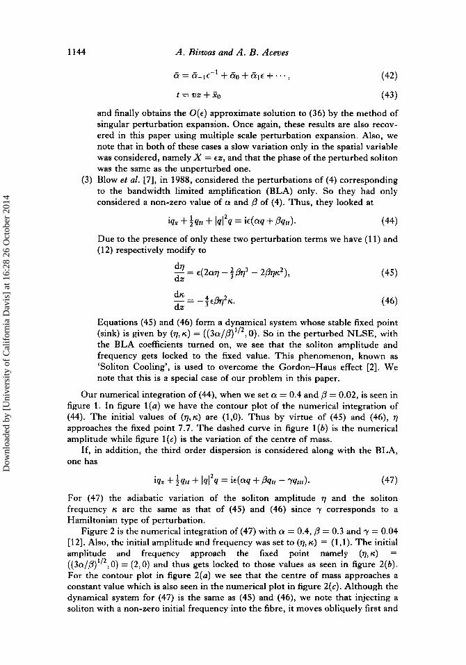
and finally obtains the O(e) approximate solution to (36) by the method of singular perturbation expansion. Once again, these results are also recovered in this paper using multiple scale perturbation expansion. Also, we note that in both of these cases a slow variation only in the spatial variable was considered, namely X = E X , and that the phase of the perturbed soliton was the same as the unperturbed one. Blow et al. [7], in 1988, considered the perturbations of (4) corresponding to the bandwidth limited amplification (BLA) only. So they had only considered a non-zero value of a and ,f3 of (4). Thus, they looked at

iqz + 3411 + 1qI2q = ie(aq + P41r). (44)

Due to the presence of only these two perturbation terms we have (1 1) and (1 2) respectively modify to

Equations (45) and (46) form a dynamical system whose stable fixed point (sink) is given by (7,~) = ( (3c~ /p )”~ ,O) . So in the perturbed NLSE, with the BLA coefficients turned on, we see that the soliton amplitude and frequency gets locked to the fixed value. This phenomenon, known as ‘Soliton Cooling’, is used to overcome the Gordon-Haus effect [2]. We note that this is a special case of our problem in this paper.

Our numerical integration of (44), when we set a = 0.4 and ,f? = 0.02, is seen in figure 1. In figure l ( a ) we have the contour plot of the numerical integration of (44). The initial values of (7,~) are (1,O). Thus by virtue of (45) and (46), 7 approaches the fixed point 7.7. The dashed curve in figure l ( b ) is the numerical amplitude while figure l(c) is the variation of the centre of mass.

If, in addition, the third order dispersion is considered along with the BLA, one has

iq, + iqtt + M 2 q = iE(aq + Pqtt - w t t t ) . (47)

For (47) the adiabatic variation of the soliton amplitude 71 and the soliton frequency K are the same as that of (45) and (46) since y corresponds to a Hamiltonian type of perturbation.

Figure 2 is the numerical integration of (47) with (Y = 0.4, p = 0.3 and y = 0.04 [12]. Also, the initial amplitude and frequency was set to (7, K ) = (1,l) . The initial amplitude and frequency approach the fixed point namely (7,~) = ( ( 3 ~ ~ / / 3 ) ~ ’ ~ , 0 ) = (2,O) and thus gets locked to those values as seen in figure 2(b). For the contour plot in figure 2(a) we see that the centre of mass approaches a constant value which is also seen in the numerical plot in figure 2(c). Although the dynamical system for (47) is the same as (45) and (46), we note that injecting a soliton with a non-zero initial frequency into the fibre, it moves obliquely first and

Dow

nloa

ded

by [

Uni

vers

ity o

f C

alif

orni

a D

avis

] at

16:

28 2

6 O

ctob

er 2

014


(4

a = 0.4 and ,O = 0.02. (c) Variation of centre of mass. Figure 1 . ( a ) Contour plot for a = 0.4 and ,O = 0.02. ( b ) Variation of amplitude for

Dow

nloa

ded

by [

Uni

vers

ity o

f C

alif

orni

a D

avis

] at

16:

28 2

6 O

ctob

er 2

014

1146 A. Biswas and A . B. Acmes

(4 Figure 2. (a) Contour plot for a = 0.4, /3 = 0.3 and y = 0.04. (b ) Variation of amplitude

for a = 0.4, /3 = 0.3 and y = 0.04. (c) Variation of centre of mass for a = 0.4, /3= 0.3 and y = 0.04

Dow

nloa

ded

by [

Uni

vers

ity o

f C

alif

orni

a D

avis

] at

16:

28 2

6 O

ctob

er 2

014

Dynamics of solitons in optical Jibres 1147

eventually moves straight as the soliton velocity gradually goes to zero, figure 2(b ) . Also, for non-zero y here we see that there is no change as it is a Hamiltonian perturbation.

(4) Kodama et al. [5] studied (4) with only the third order dispersion, namely

(48) 1 2 iqz + 2qtt + IQI q = - i w t t t ,

which is a Hamiltonian type perturbation. Here, the authors introduced the Lie transform:

Q = q - 3 i ~ y [ qt + 2q J’ -a3 1q( T ) l 2 di] ,

which transformed (48) to

(49)

But (50), with the right hand side equal to zero, is the Schrodinger-Hirota equation and is integrable by the IST. The 1-soliton solution of (SO), with the right hand side set to zero, obtained by Kodama et al., is

Q(z, t ) = 77 sech [r](t - vz - to)] exp ( -k t + iwz + ioo),

v = - 6 f € Y ( r ] - 31E )

(51)

( 5 2 )

where the velocity and the wave number of the soliton are respectively: 2 2

and

772 - 1E2 w=- + Ey6( 3772 - 62).

2 (53)

These results have been recovered here in this paper by the method of multiple scale perturbation expansion.

In figure 3, which is a contour plot, we consider the numerical integration of (48) with y = 0.14. We start with an initial amplitude and frequency r] = 1 and 1~ = 0 respectively. We note that y being a Hamiltonian perturbation, the amplitude should not change. Figure 3(b) shows the variation of the amplitude and figure 3(c) is the variation of the centre of mass of the soliton that is in agreement with (14).

When all the Hamiltonian perturbation terms of (4) are turned on we get

(54) 2

iqz + t 4 t t + 141 Q = i4X(lql2q)t + v(14I2)t4 - YQttt).

Here Kodama [3, 91 introduced the Lie transform:

Q = q - 4 3 7 +$X)qt - 4 6 7 + 2X + v ) q f I ~ ( T ) [ ~ d r (55) -W

which is a generalization of (49). Now (55) transformed (54) to (50) from which one again recovers (51), (52) and (53). Once again, these are also recovered here using the multiple scale technique.

Finally figure 4(a) is the contour plot of the numerical integration of (54) with X = 0.3, v = 0.16 and y = 0.14 [13]. While figures 4(a) and (b ) are the contour plot and the amplitude variations respectively, figure 4(c) shows the variation of the centre of mass. The slope of the straight line in figure 4(c) coincides with the value given by (14).

Dow

nloa

ded

by [

Uni

vers

ity o

f C

alif

orni

a D

avis

] at

16:

28 2

6 O

ctob

er 2

014

1148

- 0 8 -

- 0 7 -

-0 8O 10 20 M 40 50

A. Biswas and A. B . Acmes

60

Figure 3. for y = 0.14.

Dow

nloa

ded

by [

Uni

vers

ity o

f C

alif

orni

a D

avis

] at

16:

28 2

6 O

ctob

er 2

014


Figure 4. Contour plot for 7 = 0.14, X = 0.3 and u = 0.16. (b ) Variation of amplitude for 7 = 0.14, X = 0.3 and v = 0.16. (c) Centre of mass variation for 7 = 0.14, X = 0.3 and

v = 0.16

Dow

nloa

ded

by [

Uni

vers

ity o

f C

alif

orni

a D

avis

] at

16:

28 2

6 O

ctob

er 2

014

1150 Dynamics of solitons in optical fibres

Thus, we see that the multiple scale perturbation method is advantageous over the standard soliton perturbation theory (SPT). In the latter method one can only get the adiabatic variation of the soliton parameters, such as the amplitude, frequency and the O(E) variation of the soliton velocity, in presence of the perturbation terms. These are seen in (ll), (12) and (14) respectively. However, in the multiple scale technique we get the O(E) variation of the soliton frequency and wave number due to the Hamiltonian perturbations as seen in (25) and (27), which cannot be recovered by SPT. Moreover, the multiple-scale approach gives the ‘closed’ form of the perturbed soliton, given by (35), up to O(E) which is also a failure in the SPT. Also, using the multiple scale approach, which is a generalization to other approaches [2, 6, 101, one can see the variation of soliton parameters with respect to both the independent variables, namely z and t, in (18), (19), (24), (25) and (28). This is also not possible in SPT. Finally, once again, we note that the multiple-scale method is applicable to both Hamiltonian and non- Hamiltonian perturbations [9] unlike the Lie transform which is applicable only to Hamiltonian type perturbations [2, 4, 51.

6. Conclusions This paper is the study of a single soliton governed by the perturbed NLSE.

We have shown that by a proper choice of the dominant amplitude and phase of the perturbed soliton the adiabatic dynamics can be captured for most perturbations. This conclusion is based on comparison with other methods that apply to specific perturbations as well as with numerical simulations.

Acknowledgments The authors are thankful to AFOSR for their continous support.

References [l] AGRAWAL, G. P., 1995, Nonlinear Fiber Optics (San Deigo: Academic Press). [2] HASEGAWA, A., and KODAMA, Y . , 1995, Solitons in Optical Communications (Oxford:

[3] KODAMA, Y., and HASEGAWA, A., 1992, Progr. Optics, XXX, 205. [4] WABNITZ, S., KODAMA, Y., and ACEVES, A. B., 1995, Opt . Fiber Technol., 1, 187. [5] KODAMA, Y., RAMAGNOLI, M., WABNITZ, S., and MIDRIO, M., 1994, Optics Lett., 19,

[6] ABLOWITZ, M. J . , and SEGUR, H., 1981, Solitons and the Inverse Scattering Transform,

[7] BLOW, K. J . , DORAN, N. J . , and WOOD, D. , 1988, J . opt. SOC. Am. B, 5, 1301. [8] KODAMA, Y., 1985, J . stat. Phys., 39, 597. [9] BISWAS, A., 1999, J. nonlinear opt. Phys. Mat . , 8, 277.

Oxford University Press).

165.

(Philadelphia: SIAM).

[lo] KODAMA, Y., and ABLOWTIZ, M. J . , 1981, Studies appl. Math., 64, 225. [ll] KAUP, D. J . , 1990, Phys. Rew. A, 42, 5689. [12] POTASEK, M. J., 1989, J . appl. Phys., 65, 941. [13] KODAMA, Y., and HASECAWA, A., 1992, Optics Lett . , 17, 31. [14] MECOZZI, A., MOORES, J . D., HAUS, H. A., and LAI, Y., 1991, Optics Lett., 16, 1841. [15] MOORES, J . D. , WONG, W. S., and HAUS, H. A., 1994, Optics Commun., 113, 153.

Dow

nloa

ded

by [

Uni

vers

ity o

f C

alif

orni

a D

avis

] at

16:

28 2

6 O

ctob

er 2

014

Documents

Dynamics of solitons in optical fibres