Dynamics of Differential Equations

Dynamics of Differential Equations

Prof. R.S. Mackay

Lent 1997

These notes are maintained by Paul Metcalfe.Comments and corrections [email protected] .

Revision: 2.6Date: 2004/07/26 07:41:24

The following people have maintained these notes.

– date Paul Metcalfe

Contents

Introduction v

1 Differential Equations 11.1 The Problem . . . . . . . . . . . . . . . . . . . . . . . . . . . . . . . 11.2 The Traditional Approach . . . . . . . . . . . . . . . . . . . . . . . . 11.3 The Geometric Approach . . . . . . . . . . . . . . . . . . . . . . . . 21.4 Basic Theorem of ODE’s . . . . . . . . . . . . . . . . . . . . . . . . 3

1.4.1 Existance, uniqueness and continuity wrt initial conditions . . 31.5 Interval of definition of solutions . . . . . . . . . . . . . . . . . . . . 4

2 Basic Examples and Ideas 72.1 The Ideal Pendulum . . . . . . . . . . . . . . . . . . . . . . . . . . . 72.2 The Damped Pendulum . . . . . . . . . . . . . . . . . . . . . . . . . 8

2.2.1 The effect of nonlinearity on stability of equilibria . . . . . . 92.2.2 Equivalence of “attracting” and “asymptotically stable” . . . . 10

2.3 Damped Pendulum with torque . . . . . . . . . . . . . . . . . . . . . 122.3.1 The Poincare - Bendixson Theorem . . . . . . . . . . . . . . 13

2.4 The van der Pol equation . . . . . . . . . . . . . . . . . . . . . . . . 202.4.1 Topics arising from the van der Pol equation . . . . . . . . . 21

3 Bifurcations of 2D flows 253.1 Structural stability . . . . . . . . . . . . . . . . . . . . . . . . . . . . 253.2 Saddle-node equilibria . . . . . . . . . . . . . . . . . . . . . . . . . 263.3 Other cases of degenerate equilibria . . . . . . . . . . . . . . . . . . 29

3.3.1 Imperfections . . . . . . . . . . . . . . . . . . . . . . . . . . 293.4 Hopf Bifurcation . . . . . . . . . . . . . . . . . . . . . . . . . . . . 303.5 Homoclinic Bifurcation . . . . . . . . . . . . . . . . . . . . . . . . . 32

3.5.1 Finding homoclinic bifurcations in nearly Hamiltonian systems 343.6 Saddle-node of periodic orbits . . . . . . . . . . . . . . . . . . . . . 36

4 Introduction to dynamics in 3D 374.1 Time-T map . . . . . . . . . . . . . . . . . . . . . . . . . . . . . . . 374.2 Existence of periodic orbits . . . . . . . . . . . . . . . . . . . . . . . 384.3 Linear stability . . . . . . . . . . . . . . . . . . . . . . . . . . . . . 39

4.3.1 The Mathieu Equation . . . . . . . . . . . . . . . . . . . . . 404.4 Near-identity maps and averaging . . . . . . . . . . . . . . . . . . . 41

4.4.1 Application of averaging to the periodically forced van der Polequation . . . . . . . . . . . . . . . . . . . . . . . . . . . . . 42

iii

iv CONTENTS

4.5 Differences from autonomous systems . . . . . . . . . . . . . . . . . 43

Introduction

These notes are based on the course “Dynamics of Differential Equations” given byProf. R.S. Mackay in Cambridge in the Lent Term 1997. These typeset notes are totallyunconnected with Prof. Mackay. Note that these notes are based on the first year of thecourse. More material was lectured in 1998.

Other sets of notes are available for different courses. At the time of typing thesecourses were:

Probability Discrete MathematicsAnalysis Further AnalysisMethods Quantum MechanicsFluid Dynamics 1 Quadratic MathematicsGeometry Dynamics of D.E.’sFoundations of QM ElectrodynamicsMethods of Math. Phys Fluid Dynamics 2Waves (etc.) Statistical PhysicsGeneral Relativity Dynamical SystemsCombinatorics Bifurcations in Nonlinear Convection

They may be downloaded from

http://www.istari.ucam.org/maths/ .

v

http://www.istari.ucam.org/maths/

vi INTRODUCTION

Chapter 1

Differential Equations

1.1 The Problem

In this course,differential equationmeans a system of equations of the form

dxi

dt= vi(x(t)),

with x ∈ Rn, t ∈ R andvi : Rn 7→ R.1

In this course, we only study ordinary differential equations, as opposed to partialdifferential equations. More precisely, we studyautonomousODE’s, those with noexplicit time dependence inv. (Or the equation is invariant under a shift of the originin time.)

A restriction to autonomous DE’s is not that much of a restriction, since the non-autonomous systemx = f(x, t) can be reduced to the autonomous systemx = f(x, τ),τ = 1.

We also restrict to coupled first-order ODE’s. This again is little of a restriction –many higher order systems can be reduced to the first-order case, since ifx = f(x, x),then introducey = x to get the coupled systemy = f(x, y), x = y.

We also only considerexplicitsystems, but if we have the implicit systemg(x, x) =0, andx0, y0 such thatg(x0, v0) = 0, and the matrix

(∂gi

∂xj

)is invertible at(x0, v0)

then∃v : U 7→ Rn on a neighbourhoodU of x0 such that for(x, x) near(x0, v0),g(x, x) = 0 ⇔ x = v(x).

1.2 The Traditional Approach

Givenv in terms of “elementary” functions, look for a general solution ofx = v(x) interms of elementary functions. This has some drawbacks, not least of which is that itis frequently hard to do (read impossible). We also need some valid definition of ele-mentary function. And in any case the nicest definition of some elementary functionsis as the solution of certain ODE’s, for example

1. exp(t) is the solution ofx = x with x(0) = 1. The propertyexp(s + t) =exp(s) exp(t) is easy to derive – the ODE is autonomous soexp(s+t) is the solu-tion after timet starting atexp(s). But the ODE is linear, so this isexp(s) exp(t).

1Underlining of vectors will be sporadic in these notes.

1

2 CHAPTER 1. DIFFERENTIAL EQUATIONS

2. [sin tcos t

]is the solution of [

xy

]=[

y−x

]with the initial conditionsx(0) = 0, y(0) = 0. Periodicity is easy to derive -just note thatH = (x2 + y2)/2 is conserved. Thus solutions remain on the unitcircle. The direction of rotation is constant, at constant speed. So(x(t), y(t))must return to its initial conditions at someT > 0 (choose the least such). Thenby autonomy,(x(t + T ), y(t + T )) = (x(t), y(t)). Traditionally, setT = 2π,as a definition ofπ. So the traditional approach is (ahem) circular.

Even if you allow solutions of (algebraic) equations in elementary functions andintegrals of elementary functions, there are still some equations which cannot be solved(e.g. y = y2−t). Thus we try a different approach — to see what happens to solutions.

1.3 The Geometric Approach

This is due to Poincare. It has two senses.

pictorial

Let v define a vector field on a state spaceX = Rn (or more generally on somedifferentiable manifold, egS1 × R, S2, Π2 = S1 × S1). Under suitable conditions,x = v(x) defines a flowφ : R×X 7→ X, (t, x0) 7→ φt(x0), the solution at timet withx(0) = x0. A picture showing how “all” the solutions move inX is called a phaseportrait. These are hard to draw whenn > 3, but we shall restrict ton = 2 or n = 3.2

Kleinian

For Klein, the geometrical approach to a set of objects is to identify a group of trans-formations of the objects which we regard as taking each object to an equivalent oneand then studying the properties which are invariant under the group action.

The objects we will look at are the vector fieldsv on X with their associated dif-ferential equationx = v(x). The transformations we will use are change of variablesand time rescaling.

For change of variables, lety = h(x), with h a diffeomorphism. In this case,y = Dhh−1(y)v(h−1(y)), whereDh is the matrix of partial derivatives∂hi

∂xj.

For time rescaling, letdsdt = α(x) > 0, which implies thatdx

ds = v(x)/α(x).We will study the features ofx = v(x) which are preserved by the group generated

by these kinds of transformations, for instance existance of a periodic orbit (but not itsformula or period).

The geometric approach does not try to obtain as much as the traditional approach,but can get useful results where the traditional approach gets stuck.

2I have problems whenn = 3, let alone anything higher.

1.4. BASIC THEOREM OF ODE’S 3

1.4 Basic Theorem of ODE’s

We would like to justify the idea of a flow with some sort of existance and uniquenessresults.

Definition. A mapf : M1 7→ M2 between metric spaces with metricsd1 and d2 isLipschitz if ∃ L ∈ R such that∀ x, y ∈ M1, d2 (f(x), f(y)) ≤ Ld1 (x, y). L is said tobe aLipschitz constant.

Example

A mapf : U 7→ Rm, U open inRn is C1 (continuously differentiable) if

1. it is differentiable, that is∃ a linear mapDfx : Rn 7→ Rm such that

|f(x + h)− f(x)−Dfxh| = o(|h|).

2. Dfx depends continuously onx with respect to the operator norm‖Dfx‖ =suph6=0

|Dfxh||h| .

Thenf is Lipschitz on any convex compact setK ⊂ U , with Lipschitz constantL = ‖Dfx‖.

Proof. Givenx, y ∈ K, let z(s) = x + s(y − x) for 0 ≤ s ≤ 1. Then

|f(y)− f(x)| =∣∣∣∣∫ 1

0

dds

f(x(s)) ds

∣∣∣∣ = ∣∣∣∣∫ 1

0

Dfx(s)(y − x) ds

∣∣∣∣ ≤ K |y − x| .

1.4.1 Existance, uniqueness and continuity wrt initial conditions

Theorem (Basic Theorem of ODE’s). If v : U 7→ Rn, U open inRn, is locally Lip-schitz, then∀ y ∈ U , ∃ a neighbourhoodV of y and τ > 0 such that∀ x0 ∈ V ,∃ unique differentiable functionx : [−τ, τ ] 7→ U such thatx(0) = x0 and x(t) =v (x(t))∀ t ∈ [−τ, τ ]. Furthermore, if the solutionx(t) is denoted byφt(x0), thenφ : [−τ, τ ]× V 7→ U is Lipschitz.

Proof. 3 Giveny ∈ U , choose a neighbourhoodN = x : |y − x| ≤ b on whichv isLipschitz. LetL be the Lipschitz constant forv andK = supx∈N |v(x)|.

Now chooseτ , b′ > 0 such thatτ ≤ 1/L andb′+Kτ ≤ b. LetV = x : |x− y| ≤b′. Let

B = Lipschitz functionsx : [−τ, τ ] 7→ Rn of constantK andx(0) ∈ V .

Given functionsx, y ∈ B, let d(x, y) = supt∈[−τ,τ ] |x− y|. Then(B, d) is acomplete metric space. Now, forx0 ∈ V , define a mapPx0 : B 7→ B by

(Px0 x) (t) = x0 +∫ t

0

v(x(s)) ds.

Fixed points ofPx0 correspond to solutions ofx = v(x) with x(0) = x0. NowPx0

mapsB into itself and contractsd (by at leastLτ < 1). So by the contraction mappingprinciple,Px0 has a unique fixed pointx that depends Lipschitz continuously onx0. Itfollows thatφ : [−τ, τ ]× V 7→ U is Lipschitz.

3This should be familiar from Analysis IB.


Remarks

1. If v is C1, we can prove thatφ is C1. Similarly, if v is C1+Lip , C2, . . . , C∞,analytic, then so isφ.

2. x(t) is always one derivative smoother thatv(x), sincex = v(x).

3. If v is not locally Lipschitz thenx may fail to be unique, for instancex = |x|1/2

has solutions

x(t) =

−(2−t)2

4 0 ≤ t ≤ 20 2 ≤ t ≤ T(t−T )2

4 t ≥ T

for anyT ≥ 2.

This is the ODE for a particle sliding down a viscous slope of heighth(x) =− 2

3 |x|3/2

sgn(x).

4. We cannot takeτ = ∞, andτ may depend onx0. For instance, takex = x2,

x(0) = x0 > 0. Thusx(t) =(x−1

0 − t)−1 → ∞ ast x−1

0 . This is called“finite time blowup”. It is not just a pathology: it is suspected that for manysolutions of the Euler equations for a 3D fluid (and maybe even the Navier-

Stokes equations),supx

∣∣∣ ∂ui

∂xj

∣∣∣→∞ in finite time.

1.5 Interval of definition of solutions

There are several circumstances under which the solutionx(t) starting fromx0 is de-fined for all positive and negative time.

Theorem (Extension Theorem).Let K ⊂ X be compact andv a C1 vector field ona neighbourhood ofK. Thenφt(x0) is defined andC1 for all x0 ∈ K and all t suchthatφs(x0) ∈ K∀ 0 ≤ s ≤ t, plus a little more.

Proof. For all y ∈ K there exists a neighbourhoodVy andτy > 0 such thatφt(x0) isdefined andC1 for all x0 ∈ Vy, |t| ≤ τ . The setsVy : y ∈ K form an open coverof K, so by compactness∃ a finite subcoverVyi

: i = 1, . . . , N. Let τ = mini τyi.

Then∀ x0 ∈ K, φt(x0) exists for at least|t| ≤ τ . If φτ (x0) ∈ K then repeat argument.Thusφt(x0) is defined andC1 as long as it remains inK, and for timeτ more.

Corollary. The only way that a solution of aC1 ODE can cease to exist is to leaveevery compact set in bounded time.

We can use these results to get a couple of examples.

Example. If |v(x)| ≤ A |x| + B for someA > 0, B ≥ 0, thenφt(x) exists for alltand|φt(x)| ≤ (|x|+ B/A) exp(A |t|).

Proof. Compare withr = Ar + B onR+.

Example. If x = v(x, s), s = 1 then no solution remains in any compact set sincesis unbounded. But for any compactK ⊂ X, solutions can be extended as long as theyremain inK × R.

1.5. INTERVAL OF DEFINITION OF SOLUTIONS 5

Proof. Otherwise, letT1 be the infimum of positive times that solutions starting inK × 0 which do not cross∂K × R but which cannot be continued tot = T . ByassumptionT1 < ∞. ThenK × [−T1, T1] is compact, so we can apply the extensiontheorem and continue all solutions which do not cross∂K × [−T1, T1] to t = T1 + τ1.This is a contradiction.

We can often find a compactK which all solutions enter and remain inside. Wecould also in principle rescale time to prevent finite-time blowup. Thus we shall hence-forth assume thatφt(x0) is defined for allt.


Chapter 2

Basic Examples and Ideas

We will introduce the theory of nonlinear systems by means of various examples.

2.1 The Ideal Pendulum

This has the ODEθ + sin θ = 0. (With appropriate rescaling of time andθ to removeconstants.) Writing as a linked first order system, we obtain[

θp

]=[

p− sin θ

].

Write x = (θ, p) ∈ X, whereX is an infinite cylinder. Notice the conservation ofenergy, that is, letH = 1

2p2 − cos θ. ThenH = 0. Now, givenE ∈ R, define

ΣE = x ∈ X : H(x) = E .

Note thatx(0) ∈ ΣE ⇒ x(t) ∈ ΣE ∀t. We say thatΣE is invariant under the flow.Now, if E < −1 thenΣE = ∅. If E = −1 thenΣE = (0, 0) - it is an equilibrium

point.If −1 < E < 1, thenΣE is a closed curve. Nowv 6= 0 on ΣE . v is continuous

andΣE is compact. Thus∃ δE > 0 such that|v| ≥ δE onΣE . Also, the length ofΣE

is finite, so givenx ∈ ΣE , ∃T > 0 such thatφT (x) = x. ThusΣE is a periodic orbit.Physically, this corresponds to oscillations.

If E > 1 thenΣE is two closed curves.v is non-zero, so we have two periodicorbits. Physically, this is rotations.

If E = 1 thenΣE consists of the equilibrium pointx = (π, 0) and two orbits whichare asymptotic to the equilibrium in both positive and negative time. They are calledhomoclinicorbits to the equilibrium.

An orbit which is asymptotic to one equilibrium in positive time and another equi-librium in negative time is called aheteroclinicorbit.

Finding all the equilibria is easy — you just have to setv(x) = 0.The equilibriumθ = 0 and each of the periodic orbits arestable.

Definition. An invariant setΛ for a flow φ : R × X 7→ X is (Lyapunov) stable if∀neighbourhoodsU of Λ, ∃ a neighbourhoodV of Λ such thatx0 ∈ V ⇒ φt(x0) ∈U ∀t ≥ 0.

7

8 CHAPTER 2. BASIC EXAMPLES AND IDEAS

Notes. It’s useful to spot conserved quantities (if any exist). Some types of system forwhich there exist useful conserved quantities are frictionless mechanical systems (inwhich the Hamiltonian is conserved) and chemical reactions — numbers of atoms ofeach kind of element must be constant.

2.2 The Damped Pendulum

This has ODEθ + kθ + sin θ = 0, wherek > 0. As a linked system, we obtain[θp

]=[

p−kp− sin θ

].

Now, H = 12p2 − cos θ is no longer conserved, butH = −kp2. ThusH decreases

along solutions (except whenp = 0). H decreases strictly along all solutions excepton two equilibria atθ = 0, π.

Theorem. If H (φt(x)) < H (φs(x)) for t > s andx is not an equilibrium thenφt(x)tends to an equilibrium ast →∞.

Proof. Given x ∈ X, then P = y : H(y) ≤ H(x) is compact. Therefore(φt(x))t→∞ has a limit point (inP ). Define

ω(x) = Limit points of (φt(x))t→∞ .

Now ω(x) 6= ∅ (by compactness)1. Note thatd(φt(x), ω(x)) → 0, otherwise∃ε > 0 and tj → ∞ such that2ε ≥ d(φtj

(x), ω(x)) ≥ ε. Now Q = y : 2ε ≥d(y, ω(x) ≥ ε is compact, soφtj

(x) has a limit point inQ. This is a contradiction.Now H must be constant onω(x). Otherwise, suppose∃ξ, η ∈ ω(x) with H(ξ) <

H(η). Let ε = H(η)−H(ξ) > 0. Now ∃t1 such thatφt1(x) is close enough toξ thatH(φt1(x)) is within ε/3 of H(ξ). Now, ∃t2 > t1 such thatφt2(x) is close enough toη thatH(φt2(x)) is within ε/3 of H(η). ThusH(φt2(x)) − H(φt1(x)) ≥ ε/3 > 0andt2 > t1. This is a contradiction. Nowω(x) is invariant, since ifφtj

(x) → y, thenφtj+τ (x) → z by the continuity ofφτ .

SinceH is constant onω(x), ω(x) consists only of equilibria. In fact,ω(x) has tobe only a single equilibrium, asH(π, 0) = 1 andH(0, 0) = −1.

More generally, we have La Salle’s Invariance Principle.

Theorem (La Salle’s Invariance Principle). If H : X 7→ R is continuous, decreasingalong all solutions of a flow except at equilbria, andx0 ∈ X has a bounded orbit thenφt(x0) converges ast → ∞ to a connected subset of the set of equilibria on whichHis constant.2

The proof is left as an exercise.We now need to examine the way that the orbits approach the equilibria and which

orbits converge to which equilibrium. The first step is to perform linear stability anal-ysis of the equilibria. Linearise the system aboutθ = 0 or π, p = 0. We obtain

1ω(x) is called theω-limit set of x. Similarly, ast → −∞ there is theα-limit set. For the advancedstudent — whyα andω?

2Such a functionH is called a Lyapunov function.

2.2. THE DAMPED PENDULUM 9

(δθ

δp

)=(

0 1−c −k

)(δθδp

)wherec = cos θ = ±1.

This matrix has eigenvalues−k2 ±

√k2−4c

2 .At θ = π, c = −1, so we have real eigenvalues, one positive and one negative.

Thus we have a saddle point.At θ = 0, c = 1 so if 0 < k < 2 we have complex conjugate eigenvalues with

negative real part. This is a focus. Ifk > 2 we have a pair of negative real eigenvalues.This is a node.

We wish now to ask which features of the linearised system survive the nonlinearremainder term. In particular, does a sink attract all nearby orbits and does a saddlehave precisely two invariant curves through it?

2.2.1 The effect of nonlinearity on stability of equilibria

Definition. A sink is an equilibrium all of whose eigenvalues lie in the open left halfplane<(λ) < 0.

Definition. An invariant setΛ is attracting if it has a neighbourhoodU such thatφt(U) ⊂ U for t > 0 and

⋂t>0 φt(U) = Λ.

Lemma. If A is a linear operator on a finite-dimensional real vector spaceE, and alleigenvaluesλi of A haveα < <(λi) < β, then there is an inner product onE suchthat

α |x|2 ≤ 〈x, Ax〉 ≤ β |x|2 .

Proof. We choose a basis forE such thatA has real JNF with blocks of the forms

[λ1] [α2 −ω2

ω2 α2

]

λ3 ε...

...

... ελ3

α4 −ω4 ε 0ω4 α4 0 ε

α4 −ω4...

ω4 α4...

Now ε can be chosen arbitrarily small (by rescaling of basis vectors), so thatλ3 ±

ε ∈ [α, β] for all non-trivial blocks. Letxi be the co-ordinates with respect to thisbasis and choose the standard inner product〈x, y〉 =

∑i xiyi. The blocks contribute

additively to〈x, Ax〉 and the contributions are respectively

λ1x21

α2 |x|2

λ3 |x|2 + ε∑

xixi+1 ∈ [λ3 − ε, λ3 + ε] |x|2

α4 |x|2 + ε∑

xixi+2 ∈ [α4 − ε, α4 + ε] |x|2 ,


where|x| refers only to components in the appropriate block and the inclusion is ob-tained using Cauchy-Schwarz. Summing over the blocks we obtain the result

α |x|2 ≤ 〈x,Ax〉 ≤ β |x|2 .

Theorem. Every sink of aC1 vector field is attracting.

Proof. If all eigenvalues have<(λi) < 0 then∃b > 0 such that<(λi) < −b. Thelemma gives us an inner product with〈x, Ax〉 ≤ −b |x|2. So d

dt |x|2 = 2〈x, x〉 ≤

−2b |x|2 + o(|x|2), as x = Ax + o(|x|) as |x| → 0. Now givenc ∈ (0, b), thereexistsδ > 0 such that d

dt |x|2 ≤ −2c |x|2 for |x| ≤ δ. Let U = x : |x| ≤ δ. If

x(0) ∈ U then|x(t)|2 is non-increasing so thatx(t) remains inU . Furthermore, forx ∈ U \ 0, d

dt log |x|2 ≤ −2c, so that|x(t)| ≤ |x(0)| e−ct. Thusφt(U) ⊂ U∀t ≥ 0and

⋂t≥0 φt(U) = 0.

We can clearly assume that the stationary point is at the origin. Note that by revers-ing time, if all eigenvalues have<(λ) > 0 then0 is repelling.

Theorem. If A has an eigenvalue with<λ > 0 then0 is unstable.

Proof. If A has an eigenvalue with<λ > 0 then using JNF or otherwise decomposeE = E1 ⊕ E2 into invariant subspacesE1 andE2 such that all eigenvalues ofB1 =A |E1 have<λ > 0 and all eigenvalues ofB2 = A |E2 have<λ ≤ 0. Now, ∃a > 0such that all eigenvalues ofB1 have<λ > a. By the lemma there is an inner producton E1 such that〈x, B1x〉 ≥ a |x|2 for all x ∈ E1. Similarly,∀b > 0, there is an innerproduct onE2 such that〈y, B2y〉 ≤ b |y|2 for all y ∈ E2. Chooseb ∈ (0, a). Take thedirect sum inner product onE and writez ∈ E as(x, y), with x ∈ E1 andy ∈ E2.Thenv(x, y) = (B1x, B2y) + o(|x|).

Let C = (x, y) : |x| ≥ |y| andV (z) = 12

(|x|2 − |y|2

). Then

ddt

V (z) = 〈x, x〉 − 〈y, y〉

= 〈x, B1x〉+ o(|x| |z|)− 〈y, B2y〉+ o(|y| |z|)

≥ a |x|2 − b |y|2 + o(|z|2).

Given α ∈ (0, a − b), ∃δ > 0 such thatV ≥ |x|2 on C ∩ U whereU = z :|z| ≤ δ. So V increases along all orbits inC ∩ U \ 0. They cannot cross∂CbecauseV decreases across∂C. They cannot stay inC ∩ U for all t > 0 else by LaSalle’s Invariance Principle they converge to a set of equilibria with strictly largerVthan initially - but there are no equilibria except0 in C ∩ U becauseV increases inC ∩ U \ 0, V (0) = 0 andV (z(0)) > 0.

Thus there exist pointsz arbitrarily close to0 such thatφt(z) leavesU for somet > 0. This contradicts stability of0, hence0 is unstable.

2.2.2 Equivalence of “attracting” and “asymptotically stable”

Supposeφ : R×X 7→ X is a continuous flow on a locally compact metric spaceX.

Definition. Λ ⊂ X is attracting for φ if ∃ compactK ⊂ X such thatφt(K) ⊂intK ∀t > 0 and

⋂t≥0 φt(K) = λ.

2.2. THE DAMPED PENDULUM 11

Definition. Λ ⊂ X is (Lyapunov) stable if∀ neighbourhoodsU of Λ, ∃ a neighbour-hoodV of Λ such thatφt(V ) ⊂ U ∀t ≥ 0.

Definition. Λ ⊂ X is asymptotically stable forφ if it is stable and∃ a neighbourhoodW of Λ such that∀x ∈ W , d(φt(x),Λ) → 0 ast → +∞.

Theorem. Λ ⊂ X is attracting iff compact, invariant and asymptotically stable.

Proof of⇒. φt is continuous,K is compact, soφt(K) is compact, thereforeΛ =⋂t≥0 φt(K) is compact. Nowφs

⋂t≥0 φt(K) ⊂

⋂t≥0 φt(K) for s ≥ 0 so Λ is

forward invariant. Fors ≥ 0, φ−s(Λ) = φs

⋂t≥s φt(K) = Λ, so Λ is backward

invariant too.Now, let D(t) = supx∈K d(φt(x),Λ). Thenφt(K) nested, so thatD is non-

increasing. IfD 9 0 ast →∞ then∃ε > 0 such that∀t > 0, ∃xt ∈ φt(K) such thatd(xt,Λ) ≥ ε. Thext all lie in K = x ∈ K : d(x,Λ) ≥ ε, which is compact, sothey have a limit pointx ∈ K. Now for all s, xt ∈ φs(K) whent ≥ s, sox ∈ φs(K)and x ∈

⋂s≥0 φs(K). But d(x,Λ) ≥ ε, giving a contradiction. SoD(t) → 0 as

t → ∞. In particular,d(φt(x),Λ) → 0 as t → ∞ for all x ∈ K. Also, for allneighbourhoodsU of Λ, ∃T such thatφt(K) ⊂ U for all t ≥ T — or alternativelysuch thatD(T ) < infx/∈U d(x, Λ), which is positive by the compactness ofΛ. LetV = φT (K). It is a neighbourhood ofΛ because∀t > 0 Λ ⊂ φt(V ) ⊂ intV . ThusΛis stable.

Proof of⇐. Let Λε = x ∈ X : d(x,Λ) ≤ ε andW be a neighbourhood ofΛ. ThenΛ compact gives∃ε0 > 0 such thatΛε ⊂ W ∀ε ≤ ε0. Givenε ≤ ε0, there exists aneighbourhoodV of Λ such thatφt(V ) ⊂ Λ ε

2for all t ≥ 0 (Λ stable).

Also d(φt(x,Λ)) → 0 ∀x ∈ Λε, so∀x0 ∈ Λε ∃t0 and an open neighbourhoodN ofx0 such thatφt0(x) ∈ intV ∀x ∈ N (asφt0 is continuous). Soφt(x) ∈ Λ ε

2∀t ≥ t0.

The neighbourhoodsN form an open cover of the compactΛε, so finitely many suffice.Let T (ε) = maxi ti. Thenφt(Λε) ⊂ Λ ε

2for all t ≥ T (ε). So by iteration∃Tn(ε) such

thatφt(Λε) ⊂ Λ ε2n for all t ≥ Tn(ε).

Then we defineD : W 7→ R+ by D(x) = supt≥0 d(φt(x),Λ). If D(x) > 0 then∃t1(x) > 0 such thatd(φt(x),Λ) ≤ 1

2D(x) for all t ≥ t1(x). Then for ally nearenough tox the supremum ofd(φt(y),Λ) is attained in[0, t1(x)] andD is continuousatx.

If D(x) = 0 thenx ∈ Λ (by compactness) and∀ε > 0 there exists a neighbourhoodV of Λ such thaty ∈ V ⇒ d(φt(y),Λ) ≤ ε ∀t > 0 (Λ stable). SoD(y) < ε for y ∈ VandD is continuous atx.

D is non-increasing along orbits and goes to zero along each orbit. Letw =infx/∈W d(x, Λ) > 0 by compactness ofΛ. Let K = x ∈ W : D(x) ≤ w

2 is compact,φt(K) ∈ K ∀t > 0 and

⋂t≥0 φt(K) = Λ, becauseK ⊂ Λw

2and

φt(Λw2) ⊂ Λ w2n for t ≥ someTn, so d(x,Λ) = 0 for all x ∈

⋂t≥0 φt(K) so

x ∈ Λ asΛ is compact, and conversely eachx ∈ Λ lies inφt(K) for all t ≥ 0 becauseΛ is negatively invariant. To achieveφt(K) ⊂ intK ∀t > 0 we modifyD to

D∗(x) =∫ ∞

0

e−sD(φs(x)) ds.

ThenD∗ is decreasing along orbits except onΛ. So definingK = x ∈ W : D∗(x) ≤w2 we obtainΛ attracting.


1. An equivalent definition ofΛ attracting is:∃ a compact neighbourhoodK of Λsuch thatφt(K) ⊂ K for all t ≥ 0 and

⋂t≥0 φt(K) = Λ. One way to prove

the equivalence is to show that this second definition is equivalent to compact,invariant and asymptotically stable. The proof of stability works as before andthe proof of⇐ gives a neighbourhoodK.

2. Similarly, it is equivalent to require either “∃ compactK ⊂ X andT > 0 suchthatφT (K) ⊂ intK and

⋂t≥0 φt(K) = Λ” or “∃ compact neighbourhoodK

andT > 0 such thatφT (K) ⊂ K and⋂

t≥0 φt(K) = Λ”.

2.3 Damped Pendulum with torque

This has the ODEθ + kθ + sin θ = F , with k, F > 0. The equivalent linked system is

θ = p

p = −kp− sin θ + F.

Alternative motivations for this differential equation come from AC electricity gen-eration and the Josephson junction with steady current.

Again, we investigate howH = 12p2− cos θ changes with time.H = −kp2 + Fp,

which is< 0 for p outside[0, F/k] but > 0 for p in (0, F/k). H is still useful. LetE = maxp∈[0,F/k] H(θ, p) and choose anyE′ > E.

Proposition. For all x0, φt(x0) eventually entersH < E′ and stays there foreverafter. SoH acts as a “bounding function”.

Proof. If H(x) > E then H < 0. Let M = inft≥0 H(φt(x)). If M > E′ thenthe flows must converge to a set of equilibria inH = M — but there are none,as equilibria must haveH = 0. So all orbits eventually enterH < E′. Once inH < E′ they cannot escape: supposeτ is the time of first escape fromH < E′for the orbit ofx. ThenH(φτ (x)) = E′. ThusH < 0 and it is not an escape but anentry — giving a contradiction.

We are left with analysing the dynamics inH < E′. We seek the equilibria,which requirep = 0 andsin θ = F . There are two equilibria ifF < 1, one inF = 1and none ifF > 1. Performing linear stability analysis gives that one equilibrium isa saddle and the other is a focus ifk2

4 <√

1− F 2 and a node ifk2

4 >√

1− F 2.The process of annihilation of saddle and node atF = 1 is called a “saddle-nodebifurcation”.

A number of questions spring to mind:

1. Where do the stable and unstable manifolds of the saddle go? The unstablemanifold (“separatrix”) is particularly important as it separates orbits which gotwo opposite ways at the saddle. A reasonable guess is that the left branch of thestable manifold goes into the sink, but what about the rest?

2. Where do the orbits go whenF > 1, when there are no equilibria to convergeto?

We will tackle the second question first. We have an annulusA = H < E′which no orbits can escape and which contains no equilibria. Imagine flattening theannulus and regarding it as a subset ofR2.

2.3. DAMPED PENDULUM WITH TORQUE 13

2.3.1 The Poincare - Bendixson Theorem

Theorem (Poincare - Bendixson Theorem).If the forward orbit ofx (o+(x)) undera C1 vector field on an open subsetU of the plane lies in a compact subset ofU for allt ≥ 0 thenω(x) is either a periodic orbit or contains an equilibrium.

Proof. Givenx with o+(x) bounded thenω(x) 6= ∅ (by compactness). Supposeω(x)contains no equilibria and takey ∈ ω(x). ω(x) is compact and invariant, soω(y) ⊂ω(x) and is non-empty. Takez ∈ ω(y). Thenz is not an equilibrium, so there exists aC1 arcΣ transverse tov throughz. Theno+(y) comes arbitrarily close toz ast goesto∞, so in particular it crossesΣ arbitrarily close toz.

If o+(y) is not periodic then successive intersections withΣ are distinct (by unique-ness in backwards time). But if the first two intersections arey1 6= y2 theno+(x) iseventually bounded away fromy (by the Jordan Curve Theorem). Soo+(y) is periodic,intersectingΣ at one point only.

Now ω(x) is invariant soo+(y) ⊂ ω(x). Take a transverse sectionΣ′ at y. Ifo+(x) intersectsΣ′ aty theno+(x) is periodic andω(x) = o+(y). Else the successiveintersectionsxn on Σ′ converge monotonically toy. The return timesτn converge tothe periodT of o+(y), so are bounded,τn < T ′. Thus givenε > 0, d(φt(xn), φt(y)) <ε for all t ∈ [0, T ′] andxn close enough toy. But o+(xn) is trapped between thepiece fromxn to xn+1 and o+(y), so d(φt(xn), o+(y)) < ε for all t ≥ 0. Thusω(x) = o+(y).

Definition. A periodic orbitγ such that∃x /∈ γ with ω(x) = γ is called a limit cycle.

We apply Poincare-Bendixson to the damped forced pendulum forF > 1 to obtainthat for allx ∈ S1 × R, ω(x) is a periodic orbit.

Now that we have the existance of a periodic orbit, we have further questions:

1. Is it unique?

2. What is the homotopy class of the periodic orbit(s)?

3. Is it (Are they) stable?

4. What if equilibria are present?

5. What are the possibilities whenω(x) contains an equilibrium?

In general uniqueness may not hold – the ideal pendulum has uncountably manyperiodic orbits. Even when true it is hard to prove, but for the damped forced pendulumit is possible. The same technique will answer questions 2 and 3. The simplest case isproblem 2.

Consider an infinitesimal parallelipiped spanned by the columns ofB moving withthe flow. The volume of the parallelipiped,V = det B.

Theorem. Under a vector fieldx = v(x),

dV

dt= (div v)V.


Proof.

detB(t + h) = det(B(t) + hDvB(t) + o(h))= detB (det(I + hDv + o(h))= detB (1 + h div v + o(h)) as required.

Theorem. div v < 0 implies no invariant sets of positive volume.

Proof. Invariance implies thatV (t) is constant, butdiv v < 0 implies thatV decreases.

Proposition. There does not exist a contractible periodic orbit for the damped forcedpendulum.

Proof. Such an orbit bounds an invariant disk of areaA > 0. But div v = −k < 0,giving a contradiction.

We must also have at most one non-contractible periodic orbit, for the area betweentwo non-contractible periodic orbits is an invariant annulus.

We now have the negative divergence test (or Dulac criterion) for non-existance ofperiodic orbits for 2D vector fields. It is clear thatdiv v > 0 is just as good, and so isdiv(gv) ≷ 0 for g > 0, as

M =∫

Ω

g dV is a “mass” onΩ.

Theorem. div v < 0 in 2D also implies that periodic orbits are attracting.

Proof. Given a periodic orbitγ such thatdiv v < 0 in a neighbourhood ofγ choose atransverse arcΣ to γ. Then, by continuity ofφ, the forward orbits of points ofΣ nearγ(0) come back toΣ close toγ(0). In fact, bydiv v < 0 they come back closer by afactore

R T0 div v(γ(t)) dt, whereT is the period ofγ. We prove this as follows.

Take a volumeA formed by letting an arcI from γ(0) onΣ flow for a timeε > 0.After a timeT we obtain a skewed parallelogram fromA. The areaA satisfies

A(T )A(0)

∼ eR T0 div v(γ(t)) dt,

so the height must decrease as the base stays the same length – so

|I ′||I|

∼ eR T0 div v(γ(t)) dt < 1.

Now choose an intervalJ ⊂ Σ small enough so the above applies. LetU be theregion swept out byφt(J). Thenφt(U) ⊂ U for all t ≥ 0. After a timeT + δ,φt(U) ⊂ U ′, which is the analog ofU , but started fromJ ′, the first return ofJ toΣ. U ′ is thinner thanU by a factor ofe

Rdiv v dt. Thus

⋂t≥0 φt(U) = γ andγ is

attracting.


We will come across other ways of testing for homotopy class, uniqueness andstability, but the negative divergence test is easiest if it works.

For the damped forced pendulum withF > 1, for all x ∈ S1 × R, ω(x) is aperiodic orbit and is the same for allx ∈ S1 × R. We can get more information aboutit by considering “nullclines”, curves on whichθ = 0 or p = 0.

Which direction does the periodic orbit rotate?θ = 0 iff p = 0 and p = 0 iffp = F−sin θ

k . We obtain this picture.


γ ⊂ p > 0 becausep(0) < 0 implies thatp increases until positive and can nevergo negative again. Thusθ > 0 onγ. By periodicityγ spends some time inH < 0 andsome inH > 0, as

∫γ

H dt = 0. It spends some time inp > 0 and some inp < 0.What about0 < F < 1? It is important to decide where the stable and unstable

manifolds of the saddle go.

W+D must exit the annulusH < E′ downwards andW−

L goes at least to thep = 0 nullcline. There are three possible cases for the phase portrait, determined byW+

U

1. W+U hitsp = 0.

2. W+U escapes annulus.

3. W+U remains in annulus and converges to saddle after one revolution.


The first case happens with smallk, becausek = 0 conservesH = 12p2 − cos θ −

Fθ. This is the phase portrait.

W+U hits p = 0 and hence does so for all nearbyk. The second case occurs fork

large. If we rescale time by puttings = kt, then

dθ

ds=

p

kdp

ds= −p +

F − sin θ

k.

But k is large, so we getdθds = 0 and dp

ds = −p.Both the first two cases are open, meaning that(k, F ) ∈ (0,∞) × (0, 1) :

case 1 (case 2) is open. But(0,∞) × (0, 1) is connected, so case 3 occurs in be-tween. In case 3 we get homoclinic orbits — those whoseα andω limit sets con-sist of equilibria but are not themselves equilibria. For allx above the homoclinic,ω(x) = homoclinic∪ saddle.

WhenF = 1 we have a “saddle-node” instead of the saddle and sink. It has JNF[0 00 −k

]and the linearised system has a line of equilibria. The generic phase portrait near asaddle-node equilibrium is

• one sided stable manifoldW− (1D)


• half plane stable manifoldW+ (2D)

• two sided strong stable manifoldW++ (1D)

Definition. A strong stable manifold is a setx : d(φt(x), 0) ≤ d(x, 0)e−αt

for α > 0 small enough.

(We have the time reversed picture if the non-zero eigenvalue is positive.)For the damped pendulum with torqueF = 1 we obtain 3 cases according to the

behaviour ofW++U . See the next page for the pictures.

ForF = 1 andk large we have a homoclinic to the saddle-node.

Crossing either of the curves where there is a homoclinc to the saddle-node orsaddle generates (or destroys) a periodic orbit in a “homoclinic bifurcation”.

Theorem (Extension of Poincare-Bendixson). If v is a planarC1 vector field ando+(x) is bounded thenω(x) is non-empty, compact, connected and either a periodicorbit or the union of a non-empty compact set of equilibriaE and a possibly empty setof trajectories whoseα andω limit sets lie inE.

Proof. It is enough to consider the case whereω(x) contains both an equilibrium anda non-equilibrium. Call the non-equilibriumγ(0) and its trajectoryγ. Thenω(γ)consists of equilibria, else isq ∈ ω(γ) is not an equilibrium we can take a transversearcΣ throughq andγ ∩ Σ = q by the same argument as before andγ is a periodicorbit. But thenω(x) = γ by the same argument as before. Similiarlyα(x) consists ofequilibria.


The damped forced pendulum


2.4 The van der Pol equation

This is

x + (x2 − β)x + x = 0, β > 0.

Damping is positive for|x| >√

β and negative for|x| <√

β. A generalisation isthe systemx + f(x)x + g(x) = 0.

We could write it as a system usingy = x, but it is more usual to introducey =x + F (x), whereF (x) =

∫ x

0f(x) dx. Then

x = y − F (x)y = −g(x).

This reflects the original motivation: an electronic oscillator. We find the equilibriaatg(x) = 0 andy = F (x).

For the van der Pol equation there is one equilbrium at the origin, a repelling focusfor 0 < β < 2 or repelling node forβ > 2.

Every non-zero orbit moves from quadrant to quadrant clockwise. We try to find abounding function (H such thatH is decreasing when large andH is bounded below).We try H = 1

2y2 + G(x), whereG(x) =∫ x

0g(x) dx. Now H = −g(x)F (x), soH

does not provide a bounding function, though it does tell us that the origin is repelling.It will be useful to consider the change∆H is H per half revolution.

We will assume thatg(0) = 0, g′(x) > 0, f(0) < 0, f ′(x) ≥ C > 0 so thatF (x)has precisely three zeroes ata < 0 < b.

2.4. THE VAN DER POL EQUATION 21

Let Y1 be the first intersection of the backwards orbit of(b, 0) with they axis. ForY ≥ Y1 the forward orbit of(0, Y ) must enterx ≥ b and hit the negativey axis aty′.

∆HY Y ′ =∫

H dt

=∫−g(x)F (x) dt.

We will break the path into three pieces.

∆HY B =∫ b

0

−g(x)F (x)y − F (x)

dx

=∫ b

0

g(x)1− y

F (x)

dx

> 0 but decreases atY increases. The same holds forHB′Y ′ .

∆HBB′ =∫−g(x)F (x) dt

= −∫ B

B′F (x) dy

< 0 and decreases to−∞ asY increases.

Hence∆HY Y ′ decreases to−∞ asY increases and starts positive aty = Y1. Itthus has a unique zeroY0 in between. If we assume further thatg andF are bothodd then the phase portrait is symmetric with respect to reflection iny = −x and sothe unique zero corresponds to a unique periodic orbit. It attracts the orbit of all non-zero points because they must cross they axis and thenH is driven monotonically toH0 = H(0, Y0) at successive intersections.

If we do not assume odd symmetry then we need to consider the full revolutionto the positivey axis. If we letY2 be the first intersection with the positivey axisof the backward orbit from(a, 0) then forY > max Y1, Y2 we can divide the orbitinto five pieces and deduce that∆Hone revolutiondecreases asY increases. Also, for0 < Y ≤ minY1, Y2, ∆H > 0. Thus there must be a zero of∆H > 0, but we can nolonger be sure that it is unique. In general the question of the number of periodic orbitsis hard.

2.4.1 Topics arising from the van der Pol equation

Hopf bifurcation

As β decreases through zero our periodic orbit shrinks to0 atβ = 0 and is annihilated.Similarly the source at0 turns into a sink which attracts all orbits.


This is called Hopf bifurcation (Andronov, Poincare). It is very common, for in-stance feedback in a PA system as gain is increased, singing wires in the wind as speedpasses a critical value.

Nearly conservative systems

For β small it is only interesting to considerx small since energy decreases for largeamplitude (x ∼

√β). Then the equation is close to the harmonic oscillatorx + x = 0.

We can use this to determine the approximate size and shape of the periodic orbit. Wecompute∆H =

∮−g(x)F (x) dt around a periodic orbit of the harmonic oscillator

with radiusr.

∆H =∮−r cos t

(r3

3cos3 t− βr cos t

)dt

= πr2

(β − r2

4

).

To first order inβ we expect the periodic orbit of the van der Pol oscillator to beclose to the periodic orbit of the harmonic oscillator for which∆H = 0, thusr ≈ 2

√β

andT ≈ 2π.

Relaxation Oscillators

Forβ large, what is the periodic orbit? We rescalex by√

β andy by β32 to obtain

x = β

(y − x3

3

)+ x

y = −x

β.

If β is large thenx is large unlessy ≈ x3

3 − x. Theny = −xβ gives the direction of

motion along the curve until the turning points.

We can get the approximate period by integratingdt over the slow phases:

T ≈ 2∫ 2

3

− 23

dy

y.

2.4. THE VAN DER POL EQUATION 23

We usey ≈ x3

3 − x anddy = (x2 − 1)dx. ThusT ≈ β2 (3− 2 log 2) for largeβ.

Poincare Index

Continuity of the vector field imposes strong restrictions of the possible arrangementsof equilibria and limit cycles.

Given a vector fieldsv onR2 and any simple closed curveγ on whichv 6= 0 definethe index ofγ to be the number of timesv rotates around0 for one revolution aroundγ (taken anticlockwise).

For instance, a small curve around an attracting focus has index+1 and a smallcurve around a saddle has index−1.

• Index is preserved under continuous deformations ofγ in the clan of curvessuch thatv 6= 0 on them. We can therefore defined the index of an isolatedequilibrium to be the index of all small enough curves aroung it. Attracting andrepelling foci/nodes, improper nodes, stars and centres have index+1, whereassaddles have index−1. The index of a small curve surrounding no equilibria is0.

• The index of a “sum” of closed curves is the sum of the indices.

• Hence the index ofγ is the sum of the indices of the equilibria insideγ.

• Index of a periodic orbit is+1.

So every periodic orbit must surround at least one equilibrium and the sum of theindices of the equilibria surrounded must be+1.

Floquet multipliers of a periodic orbit

Take a transverse sectionΣ to γ and letf : Σ 7→ Σ be the first return map. Thenγ(0)is a fixed point off .

Definition. λ = f ′(γ(0)) is the (Floquet) multiplier ofγ.

λ does not depend on the choice ofΣ andλ > 0 for orientable surfaces. If|λ| < 1the periodic orbit is attracting and if|λ| > 1 the periodic orbit is repelling. We say thatγ is hyperbolic is|λ| 6= 1.

In higher dimensions, the multipliers are the eigenvalues ofDfγ(0).


Chapter 3

Bifurcations of 2D flows

We have seen that the dynamics of planar vector fields is fairly simple — theω-limitsets are of limited types. There can be interesting changes in qualitative behaviour asparameters are varied (bifurcations).

3.1 Structural stability

The first step is a non-bifurcation result.

Theorem (Andronov-Pontryagin). Suppose aC1 vector fieldv points inwards onthe diskD2 ⊂ R2, flow φ all its equilibria and periodic orbits are hyperbolic andthere are no saddle connections, then the flowsφ for all C1-close vector fieldsv aretopologically equivalent, that is

φτ(t,x)(h(x)) = h(φt(x))

for some near-identity homeomorphismh : D2 7→ D2 and continuousτ : R+ ×D2 7→R+ which is an orientation-preserving homeomorphism ofR+ for eachx ∈ D2 andτ(t, φs(x)) = τ(t + s, x).

Vector fieldsv such that allC1-close v have topologically equivalent flows arecalled “structurally stable”.

Note. TheC1-norm is‖v‖1 = supx∈D2 max (|v(x)| , ‖Dv(x)‖).

We’ll prove a small part of this and then investigate what happens when any of thehypotheses are not satisfied.

Definition. An equilibriumx of a C1 vector fieldv is non-degenerate if0 is not aneigenvalue ofDvx.

Theorem (Persistence of non-degenerate equilibria).If x0 is a non-degenerate equi-librium of C1 vector fieldv0 andU is a neighbourhood ofx0 then there exists a sub-neighbourhoodV andε > 0 such that‖v − v0‖1 < ε onV implies thatv has a uniqueequilibriumx ∈ V , and it is non-degenerate and dependsC1 onv.

This is an application of the Implicit Function Theorem, an important result inanalysis which we will use frequently. Here is a general statement.

25

26 CHAPTER 3. BIFURCATIONS OF 2D FLOWS

Theorem (Implicit Function Theorem). LetX, Y andZ be open subsets of completenormed vector spaces andF : X × Y 7→ Z be C1. SupposeF (x0, y0) = z0 and∂F∂x : X 7→ Z is invertible there. Then for all small enough neighbourhoodsV of x0

there exists a neighbourhoodW of y0 such thaty ∈ W implies that∃!x(y) ∈ Vwith F (x(y), y) = z0. Furthermore,∂F

∂x is invertible at(x(y), y) and the mapping

x : W 7→ V is C1, with dxdy = −

[∂F∂x

]−1 ∂F∂y .

We will not prove this here, but we will apply it to three cases.

Persistence of Equilibria

Given aC1 vector fieldv on Rn, let F (x, v) = v(x), F : Rn × “C1 vector fields” 7→Rn. If we have a vector fieldv0 and equilibriumx0, F (x0, v0) = 0. If ∂F

∂x is invertibleat (x0, v0) then there is a locally unique equilibriumx(v) for eachv nearv0. Weconclude by saying that∂F

∂x = ∂v∂x is invertible if no eigenvalue is0.

Return map to a C1 transverse section for aC1 vector field isC1

SupposeΣ is a givenC1 transverse section tov. Suppose it is given by choosing 1co-ordinatexn for which vn is non-zero onΣ and letx′ stand for the remaining co-ordinates. ThenΣ has formxn = ζ(x′) for someC1 ζ. We can also writeΣ asx : α(x) = 0 for C1 α.

Now v induces aC1 flow φ : R× Rn 7→ Rn, t× x 7→ φt(x). Supposex ∈ Σ andφt(x) ∈ Σ for somet > 0. Then we would like to deduce that∃ C1 t(x), Σ 7→ R suchthatf(x) = φt(x)(x) ∈ Σ, so the return mapf is C1. We apply the IFT to

F : (x′, t) 7→ α(φt(x′, ζ(x′))).

Now F (x′, t) = 0 and ∂F∂t = dα v(φt(x′, ζ(x′)) 6= 0, so it is invertible. Hence there

exists a locally uniquet(x′) such thatF (x′, t(x′)) = 0. The return timet is C1.

Persistence of non-degenerate periodic orbits

Definition. A periodic orbit is non-degenerate if it has no Floquet multiplier+1.

A periodic orbit of v corresponds to a fixed point of the return mapf to sometransverse sectionΣ. Non-degenerate means that(I − Dfx) is invertible. It can beproved thatf dependsC1 onv. The equation to solve for a fixed point off if f(x, v) =x. We apply the IFT toF (x, v) = f(x, v)− x, F : Σ× “C1 vector fields”7→ Σ. Now∂F∂x is invertible, so wecanapply the IFT to get the required result.

3.2 Saddle-node equilibria

Definition. A saddle-nodeis an equilibrium with an eigenvalue0, but this does notsuffice to determine the local phase portrait. In addition we require :-

1. 0 is a simple eigenvalue (multiplicity1),

2. there is no other spectrum on the imaginary axis,

3. a non-degeneracy assumption on the quadratic part of the Taylor expansion (tobe revealed later).

3.2. SADDLE-NODE EQUILIBRIA 27

The linearised picture has a line of equilibria, which is not typical in nonlinear sys-tems. We will find that all sufficiently smooth nonlinear systems possess an invariantcurve tangent to the0-eigenvector such that the motion relative looks the same (topo-logical equivalence) as for the linear system, but the dynamics on the invariant curve isin general non-trivial. This invariant curve is called a centre manifoldW c.

Theorem (Centre manifold theorem). Given an equilibrium with some spectrum onthe imaginary axis, letEc be the span of eigenvectors corresponding to eigenvalues onthe imaginary axis and letEh be the span of eigenvectors corresponding to eigenvaluesoff the imaginary axis. Choose the corresponding co-ordinate system(c, h) and writethe vector field asc = C(c, h), h = H(c, h). Then there is a locally invariant sub-manifold of the formh = W (c) = o(|c|) and the dynamics is topologically equivalentto

c = C(c,W (c))h = ∂H

∂h |0.h.

We will not prove this theorem, but knowing the result we can computeW c to anydesired accuracy by searching for it as a Taylor series and comparing coefficients. Thegoal is to determine the dynamicsc = C(c,W (c)) onW c to sufficiently high order todetermine its topological type.

Example. x = x2 + xy + y2 = X(x, y)y = −y + x2 + xy = Y (x, y)

Solution. This is already in a good co-ordinate system,c = x andh = y. We look fory = W (x) = a2x

2 + a3x3 + a4x

4 + . . . . Invariance means that the two expressionsfor y ony = W (x) must be equal.

1. y = Y (x,W (x)) = −(a2x2 +a3x

3 +a4x4 + . . . )+x2 +x(a2x

2 +a3x3 + . . . )

2. y = ∂W∂x X(x,W (x)) = (2a2x + 3a3x

2 + . . . )(x2 + x(a2x2 + . . . ) + (a2x

2 +. . . )2).

Comparing coefficients yieldsy = x2 − x3 + o(x4) and the dynamics onW c isx = X(x, W (x)) = x2 + x3 − 2x5 + o(x5). The first term suffices to determine localtopological type and the full local phase portrait is as above.

Example (Damped pendulum withF = 1).θ = p

p = −kp− sin θ + 1

has an equilibrium at(π2 , 0) with eigenvalue0.


Solution. It is not necessary to transform to co-ordinates in whichEc andEh are axes.We just need to shift the origin to(π

2 , 0) by usingφ = θ − π2 and look for an invariant

manifold tangent toEc. We setp = a2φ2 + a3φ

3 + . . . and compare coefficients.After some fiddling we get the center manifoldp = 1

2kφ2 − 12k3 φ3 + O(φ4) with

motionφ = 12kφ2 − 1

2k3 φ3 + O(φ4). Again the local picture is determined by the firstterm.

We can now give the non-degeneracy condition referred to earlier: the quadraticpart of the vector field on the centre manifold is non-zero.

Notes. 1. Centre manifolds are in general not unique, for instancex = x2, y =−y: we can take any trajectory on the left∪ the positivex axis.

2. But they all have the same Taylor expansion.

3. There is not necessarily any analytic centre manifold, and the Taylor expansionneed not converge, or if it does the limit need not be a centre manifold.

Now we want to find out what happens to a saddle-node if we change some param-eters of the vector field. We consider the damped forced pendulum withF = 1+µ. Weadd the equationµ = 0 and compute the 2D centre manifoldp = W (φ, µ) of the ex-tended system, which should be tangent to the span of the eigenvectors and generalisedeigenvectors for eigenvalue0, that is1

00

and

01k1

.

We write p = µk + a11φ

2 + a12φµ + a22µ2 + . . . and fiddle a bit to getp =

µk + 1

2kφ2 − 1k3 φµ + 1

k5 µ2 + . . . , and the dynamics on the centre manifold isφ = µ

k + 12kφ2 + o(φ2 + |µ|)

µ = 0.

This is easy to analyse, we have a curve of equilibriaµ = − 12φ2 + o(φ2) and so

have an attracting and repelling equilibrium for eachµ < 0 and no equilibria forµ > 0.

We put in contracting dynamics in thep direction to obtain the following transition.

3.3. OTHER CASES OF DEGENERATE EQUILIBRIA 29

This is called a saddle-node bifurcation. We obtain an equivalent picture wheneverwe have a saddle-node equilibrium forµ = 0 such that the coefficienta 6= 0 in the CMflow

φ = aµ + bφ2 + o(φ2 + |µ|)µ = 0

.

3.3 Other cases of degenerate equilibria

If either a or b is zero we need to compute the flow on the centre manifold to higherorder.

The transcritical bifurcation

Here,a = 0 andb 6= 0 andx = bx2+cxµ+dµ2+O(3)with c2 > 4bd. Then we obtain two curves of equilib-ria, both transverse toµ = const and the dynamicslooks like this.

Proof. If we ignoreO(3) the equation for equilibria gives a line pair through(x, µ) =(0, 0). Write it asPQ = 0 by factorising the quadratic. Then to prove that thereis a curve of equilibria nearP = 0, for F (P,Q) = PQ + O(3) write G(R,Q) =F (RQ, Q) = RQ2 +Q3O(1) and then letH(P,Q) = G

Q2 = R+QO(1). Then∂H∂R is

invertible andH(0, 0) = 0, so by the IFT there is a locally unique solutionR = R(Q),ie P = QR(Q).

The transcritical bifurcation is common where0 is always an equilibrium.

The pitchfork bifurcation

In this casea = b = 0,

x = cxµ + dµ2 + ex3 + o(x3 + µ2),

with c, e 6= 0. There exist two curves of equilibria,x ∼ −d

c µ andµ ∼ − ecx2. This is clear if there is

no remainder, and if the remainder is present the IFTcan be applied to scaled problems forx = µξ(µ) andµ = x2ν(x).

The picture depends on the sign ofc and e. It is “supercritical” if ce < 0 —one attracting equilibrium gives two attracting and one repelling ascµ increases. It is“subcritical” if ce > 0, in this case one repelling equilibrium gives two repelling andone attracting ascµ increases.

The pitchfork is common in systems with odd symmetry,x(−x, µ) = −x(x, µ).Thena = b = d = 0.

3.3.1 Imperfections

If a one-parameter family of vector fieldsvµ has a saddle-node bifurcation and thenwe make a small change to the family, represented by an additional parameterε, thenwe can make a 3D centre manifold(x, µ, ε). (By the IFT) The curveµ ∼ − b

ax2 ofequilibria for ε = 0 persists to a curveµ ∼ − b

ax2 + εg(x, ε) for someg, but all this


does for smallε is to move the saddle-node bifurcation byO(ε) in (x, µ), giving atopologically equivalent bifurcation.

On a transcritical bifurcation

x = bx2 + cxµ + dµ2 + O(3) + εf(x, µ, ε) on the centre manifold.

We find generically one of two cases forε > 0 (depending onf ).

Lastly we consider the effect of imperfection on a pitchfork.x = cxµ + dµ2 +ex3+o(x3+µ2)+εf(x, µ, ε) on the centre manifold. Generically the pitchfork breaksas shown (or the other way!).

3.4 Hopf Bifurcation

Another way the hypotheses of Andronov-Pontryagin is if there is an equilibrium witha pair of eigenvalues on the imaginary axis. Suppose they are simple and there is noother spectrum on the imaginary axis.

Suppose we have a one-parameter family of vector fields going through this case atµ = 0. Then the equilibrium persists and moves smoothly withµ, so we could shift theorigin as a function ofµ to keep the equilibrium at0. Furthermore, simple eigenvaluesof a matrixAµ move smoothly withµ. Thus we have eigenvaluesα(µ) ± ıβ(µ) withα(0) = 0 andβ(0) 6= 0. Take a centre manifold and use polar co-ordinates(r, θ, µ).

Theorem. Supposeα′(µ) 6= 0. Then, forr small,∃ a smooth functionµ(r) : R+ 7→ Rsuch that forµ = µ(r) the orbit of(r, θ = 0) is periodic andµ(0) = 0, µ′(0) = 0.

Proof. WLOG use co-ordinates so that the linear part is[xy

]=[α(µ) −β(µ)β(µ) α(µ)

] [xy

]and WLOGα′(µ) > 0, β(µ) > 0. Then, switching to polars,r = α(µ)r + O(r2)

andθ = β(µ) + O(r). So drdθ = α(µ)

β(µ) r + O(r2). Then the return map fromθ = 0 to

3.4. HOPF BIFURCATION 31

θ = 2π is well defined:r′ = ρ(r, µ). Now ∃ a periodic orbit throughr > 0, θ = 0 iffρ(r, µ) = r. It is most convenient to write this as

F (µ, r) = log ρ(µ, r)− log r = 0.

Since ddθ log r = α

β + O(r), F (µ, r) = 2πα(µ)β(µ) + O(r), so we can extendF to

r = 0. Now F (0, 0) = 0 and ∂F∂µ (0, 0) = 2πα′(0)

β(0) 6= 0, so we can apply the IFTto deduce a locally unique curve of solutionsµ = µ(r), provided we show thatF isC1. Now F is C1 for r > 0 by the basic theorem of ODEs extended to time- andparameter-dependent vector fields. But what about atr = 0?

To tackle this we will perform some further co-ordinate changes to simplify thedifferential equations. It is easiest to do this in the complex co-ordinatez = reıθ =x + ıy. The linear part is already in the formz = λz whereλ = α + ıβ. Suppose wehave a Taylor expansion

z = λz + a11z2 + a12zz + a22z

2 + O(|z|3) a11, a12, a22 ∈ C.

We seek to eliminate the quadratic terms by change of variable

z = w + b11w2 + b12ww + b22w

2 b11, b12, b22 ∈ C.

The inverse function theorem givesw = z − b11z2 − b12zz − b22z

2 + O′(|z|3) Then(after substituting and fiddling), we find that if we choose

b11 =a11

λ

b12 =a12

λ

b22 =a22

α− 3ıβ

we eliminate all quadratic terms to obtainw = λw + O(|w|3). Now use polar co-ordinatesw = reıθ to obtain d

dθ log r = αβ + O(r2). ThenF = log ρ(µ, r)− log r =

2π α(µ)β(µ) + O(r2) is C1 at r = 0 also with ∂F

∂r = 0. So the IFT gives a locally uniquesolutionµ = µ(r) for r small andµ(0) = 0, µ′(0) = 0.

Remarks

In fact α′(µ) > 0 WLOG, and then for(µ, r) small, F (µ, r) < 0 for µ < µ(r)so intersections withθ = 0 move towards0 and forµ > µ(r), F (µ, r) > 0 andintersections withθ = 0 move away from0.

If we carry out the elimination to higher order we can determine the topologicaltype of the flows for(µ, r) small.

Supposew = λw+a111w3 +a112w

2w+a122ww2 +a222w3 +O(|w|4). We try to

eliminate all cubic terms by change of variablew = v + b111v3 + b112v

2v + b122vv2 +b222v

3. We find that we cannot eliminate all the cubic terms, the best we can do is ifwe choose

b111 =a111

2λb112 = 0

b122 =a122

2λ

b222 =a222

3λ− λ


and we reduce the equation tov = λv + av2v + O(|v|4), wherea = a112. This iscalled a “normal form”. In polars,

r = αr + <(a) r3 + O(r4)θ = β + =(a) r2 + O(r3)

,

so we expect a periodic orbit of radiusr ∼√−α(µ)<(a) .

Now ddθ log r = α+<(a) r2

β+=(a) r2 + O(r3) and

F = [log r]2πθ =

2π

β

(α + <(a) r2

)(1− =(a)

βr2

)+ O(r3).

Thus the solution curve hasµ ∼ − <(a)α′(µ)r

2. WLOGα′(µ) > 0. If <(a) < 0 we geta supercritical bifurcation and if<(a) > 0 we get a subcritical bifurcation.

3.5 Homoclinic Bifurcation

A third way in which Andronov-Pontryagin can fail is if there is a saddle connection.Let’s consider the simplest interesting case: a 2D vector field with a saddle and ahomoclinic orbit to it. Suppose this occurs atµ = 0 in a smooth one-parameter familyof vector fieldsvµ.

The saddle is hyperbolic (and therefore persistent), so we can take it at0 for allµ. It can also be proved that the local stable and unstable manifoldsW±

ε = x :d(φt(x), 0) ≤ ε ∀t ≷ 0 respectively, forε small, vary smoothly withµ, so for anyt > 0 so doφ±t andW±

ε . In particular, if we choose a transverse sectionΣ to thehomoclinic orbit atµ = 0 then the first intersections ofφ±t(W±

ε ) with Σ vary smoothlywith µ.

Choose a co-ordinates alongΣ with s+ = 0 WLOGfor all µ, oriented as shown. Assumeds−

dµ 6= 0 (WLOG> 0) and analyse the first return map froms > 0 to s′

onΣ.Clearlylims→0 s′(s) = s− ands′(s) is increasing, butresults will depend crucially on the slopeds′

ds . This isdecided by the eigenvalues of the saddle as follows.We can choose co-ordinates (depending smoothly onµ) so that the linearisation at

0 is x = −α(µ)xy = β(µ)y

, where−α < 0 andβ > 0 are the eigenvalues.

3.5. HOMOCLINIC BIFURCATION 33

Furthermore we makeW±ε go exactly along the axes

x = −xf(x, y, µ)y = yg(x, y, µ)

near0f(0, 0, µ) = αg(0, 0, µ) = β.

Then we compute the “transit map” fromx = ξ to y = η, ξ, η small.

∆ log x =∫

x

xdt =

∫x

xydy =

∫−f(x, y)

g(x, y)d(log y)

∼ −α

β∆ log y.

The slope is given byδx1ξ ∼ α

βη

(y0η

)αβ−1

. This cannot be deduced by differentia-

tion. Instead use volume changes by a factoreR

div v dt. Thus

δx1yη

δy0xξ

= eR

div v dt ∼ e(b−a)T ,

where the transit time

T =∫

dt =∫

dy

y=∫

dy

yg∼ 1

β∆ log y =

1β

logη

y0.

So δx1δy0

∼ αξβη

(y0η

)αβ−1

. Caution: the∼ is not strong

enough to deduce behaviour forα = β. To obtain thereturn map toΣ we must compose 3 maps. The firstand third are diffeomorphisms, as they are achieved inbounded time, so they do not change the power law ofthe second map. Hence we obtain:

Forα > β an attracting periodic orbit is born asµ increases through0. Forα < β arepelling periodic orbit is destroyed asµ increased through0. The caseα = β requiresfurther analysis.


The period of the periodic orbit is dominated by the time spent near the saddle. Forα > β it hasy0 ∼ Cµ for someC, soT ∼ 1

β log ηCµ → ∞ asµ 0. Forα < β it

hasx1 ∼ −Cµ, so

T =∫

dx

x∼ − 1

αlog

x1

ξ∼ 1

αlog

ξ

C |µ|→ ∞ asµ 0.

Let’s compute its Floquet multiplier. Ifα > β

slope at fixed point∼ C ′(

y0

η

)αβ−1

∼ C ′(

Cµ

η

)αβ−1

→ 0 asµ 0.

If α < β,

slope at fixed point∼ C ′(

x1

ξ

)1−αβ

∼ C ′(

C |µ|ξ

)1−αβ

→∞ asµ 0.

We define the Lyapunov (or Floquet) exponents of a periodic orbit to be the log-arithm of the Floquet multiplier divided by the period. In both the above cases theLyapunov exponent isβ − α.

Note. In 2D there is only one Lyapunov exponent and we can get it using volumechange: the Floquet multiplier ise

Rdiv v dt, so the Lyapunov exponent is1T

∮div v dt,

the average ofdiv v around the orbit.

3.5.1 Finding homoclinic bifurcations in nearly Hamiltonian sys-tems

In 2D, a Hamiltonian system is onex = ∂H

∂y

y = −∂H∂x

for someH : R2 7→ R. It automatically conservesH. If H has a saddle pointsthen it gives a saddle equilibrium forv. The level setH = H(s) often contains ahomoclinic orbit.

In a Hamiltonian system the eigenvalues−α andβ always satisfyα = β, so wecan’t immediately apply the previous results. But suppose we have a two-parameterfamily vµ,ε of the form

x =[

Hy

−Hx

]+ fµ,ε(x), f0,0 ≡ 0.

Then under suitable conditions, we will find a curve of homoclinic bifurcations in the(µ, ε) plane.

Choose a transverse sectionΣ to the homoclinic orbit of(µ, ε) = (0, 0). Then fornearby(µ, ε) the saddle persists and local stable/unstable manifolds move smoothly toobtain.

3.5. HOMOCLINIC BIFURCATION 35

Let us evaluate∆H = H(s−)−H(s+). We get a homoclinic orbit if∆Hµ,ε = 0.Now

∆H =∫ s−

s

dH

dtdt +

∫ s

s+

dH

dtdt

=

(∫ s−

s

+∫ s

s+

)(DH.fµ,ε(x) dt)

=

(∫ s−

s

+∫ s

s+

)(fµ,ε.∇H) dt.

To leading order inµ, ε we can evaluate this by integrating along the homoclinicγof µ, ε = 0. DefineM(µ, ε) =

∫γ

DH.fµ,ε(x(t)) dt. If M(µ, ε) has a curveΓ of sim-ple zeroes then use the IFT to deduce thatvµ,ε has a curve of homoclinic bifurcationsalong a nearby curveΓ.

Return to the DFP

If you’ve forgotten(!), this has equationsθ = p andp = −kp − sin θ + F . The casek = F = 0 is Hamiltonian,H(θ, p) = 1

2p2 − cos θ. This has two homoclinics to thesaddle atp = 0, θ = π (or−π) with equationsp = ±2 cos θ

2 .

M(k, F ) =∫

γ+

DH

(0

−kp + F

)dt =

∫γ+

(sin θ p

)( 0−kp + F

)dt

=∫

γ+

−kp2 + Fp dt

Now usedt = dθθ = dθ

p .

M(k, F ) =∫ π

−π

F − 2k cosθ

2dθ

= 2πF − 8k

For k > 0, note thatα > β. Thehomoclinic bifurcation generates anattracting periodic orbit.

Other cases of saddle connections:

• n-D vector field with homoclinic to hyperbolic equilibrium

• homoclinic to saddle-node

• heteroclinic cycle

• 2 homoclinics to the same saddle.


The energy method can also be used to find approximate periodic orbits for nearlyHamiltonian systems. In general, Hamiltonian systems have a family of periodic orbitslabelled by energy. Choose a transverse section and compute∆H for the first returnfor the perturbed system.

M(µ, ε, E) =∮

γ(E)

DH.fµ,ε dt,

whereγ(E) is the periodic orbit of the unperturbed system with energyE. If M has asimple zero as a function ofE thenvµ,ε has a periodic orbit nearγ(E).

3.6 Saddle-node of periodic orbits

Take a periodic orbitγ with Floquet multiplier+1. Take a transverse sectionΣ withco-ordinates. The return mapf hasf(γ(0)) = γ(0) andf ′(γ(0))′ = +1. Supposef ′′ 6= 0. If we change a parameterµ thenf changes smoothly withµ and we obtain (if∂f∂µ |0 > 0):

As µ increases through0 an attracting and a repelling fixed point collide and anni-hilate.

This is a saddle-node bifurcation of periodic orbits. We can extend this to higherdimensional vector fields by constructing a centre manifold for fixed points of the returnmapf : Σ 7→ Σ analogously to the centre manifold for equilibria.

Chapter 4

Introduction to dynamics in 3D

We restrict attention to periodically forced 2D systems, as many of the interesting phe-nomena already occur here.

For instance, the periodically forced van der Pol oscillator,x + (x2 − β)x + x =A cos ωt, which may be rewritten as

x = y − F (x)y = −x + A cos φ

φ = ω

for φ ∈ S1. Remember thatF (x) =x3

3− βx.

Or the periodically additively forced pendulum,θ + kθ + g sin θ = F + A cos ωt,which is

θ = p

p = −kp− g sin θ + F + A cos φ.

φ = ω

The parametrically forced pendulum isθ + kθ + (α + ε sinωt) sin θ = 0 may bewritten as

θ = p

p = −kp− (α + ε sinφ) sin θ,

φ = ω

a vector field onS1 × R× S1.

4.1 Time-T map

At least conceptually, dynamics of a periodically forced 2D system,x = v(x, t) =v(x, t+T ) can be reduced to iteration of a 2D mapf . Defineφs,t to be the map which,givesx(t) givenx(s), that isx(t) = φs,t(x(s)). Then letf beφ0,T , the “time-T map”.Now φ0,nT = f · · · f = fn. So we can findx(nT ) from x(0) by iterating. Also,φmT+s,nT+t = φ0,t fn−m φ−1

0,s (0 ≤ s, t < T ), so we can get from any time to anyother time by knowingf andφ0,s for s ∈ [0, T ).

The problem is that in generalf is not explicitly available. But we can often getsufficient information aboutf to determine a lot about the dynamics.

37

38 CHAPTER 4. INTRODUCTION TO DYNAMICS IN 3D

4.2 Existence of periodic orbits

The period of any periodic orbit ofx = v(x, φ), φ = 1, φ ∈ S1T is a multiple ofT .

PeriodT orbits correspond to fixed points off , periodnT orbits correspond to periodn orbits off , or fixed points offn. We therefore want the fixed points of a map. It issometimes easy.

Contraction Mapping

If f maps a closed setB into itself and contracts distances inB thenf has a uniqueattracting fixed point inB. We can often verify this even without a formula forf .

Example. We prove the existance of a periodic orbit for the van der Pol oscillator

x + (x2 − β)x + x = A cos ωt, β < 0.

Solution. We consider the Riemannian metricdl2 = dx2 + (dy − |β|2 dx)2. We find

that δl ≤ −12 |β| δl for a line element. Thusδl(T ) ≤ δl(0)e−

12 |β|T . In particular, after

one periodδl(T ) ≤ λδl(0), λ = e−12 |β|T < 1. Let K = l(f(0)). For allR ≥ K

1−λ ,f maps the disc ofl-radiusR into itself and contracts by at leastλ. Thusf has a fixedpoint inR2 which attracts all orbits. This is a “globally attracting fixed point”.

Lefschetz Index

This is the discrete-time analog of the Poincare index. Letγ be a simple closed curvewhich passes through no fixed points. Then the index ofγ underf is the number ofrevolutions off(x)− x around0 for one revolution ofx aboutγ.

If the index ofγ underf is non-zero thenγ surrounds at least one fixed point. Theindex of a small curve about a non-degenerate fixed point is(−1)# Real positive multipliers> 1.

Perturbation

If the unforced case has an equilibrium thenx = v(x), φ = 1 then this will persist forε small in the systemx = vε(x, φ), φ = 1 to give a periodic orbit.

If the equilibrium has eigenvaluesλj then the period-T orbit has multiplierseλj .The periodic orbit is therefore non-degenerate iffeλj 6= 1 ∀j.

Harmonic balance

Try Fourier series to get

x(t) =∑n∈Z

xne2πT ınt.

4.3. LINEAR STABILITY 39

Energy balance

For nearly Hamiltonian systems the method of energy balance can be used as before.

4.3 Linear stability of periodic orbits of T -periodic vec-tor fields

Given aT -periodic vector fieldx = v(x, t) and a periodic orbitγ(t) of periodT ,linearise about it to getδx = Dv(γ(t), t)δx. Write this asx = A(t)x. Let Φ(t) be thematrix solution ofΦ = A(t)Φ(t) with Φ(0) = I (the “fundamental matrix solution”).Then the solution for anyx0 is x(t) = Φ(t)x0. In particular,x(nT ) = Φ(T )nx0, sostability is determined by the eigenvalues ofΦ(T ). These are the Floquet multipliersbecauseΦ(T ) = Df , the derivative of the return map.Φ(T ) is called the “monodromymatrix”.

In the 2D case, writeΦ(t) =[a bc d

]. Then the Floquet multipliersλj are the roots

of λ2 − trλ + det = 0, that isλ± = tr2 ±

√tr2

4 − det.If both |λ±| < 1 then the periodic orbit is attracting. If one of|λ±| > 1 then

the periodic is unstable. The stability boundaries are given bytr = 1 + det, tr =−(1 + det), det = 1 andtr2 ≤ 4 det. Note thatdet = e

Htr A(t) dt > 0.

In practice,Φ(T ) is not easy to calculate unlessA(t) is constant,A(t) is piece-


wise constant orA(t) is diagonalisable by a constant matrix. But we can always getdetΦ(T ) and we can computetrΦ(T ) to any desired accuracy by perturbation from aknown case.

4.3.1 The Mathieu Equation

This isx+ kx+(α+ ε sin t)x = 0, the linearisation aboutθ = 0 of the parametricallyforced pendulum. The linked first order system is

x = y

y = −ky − (α + ε sin t)x

or x = [C + εP (t)]x. The solution forε = 0, α > 0 is

Φ(t) =[

cos ωt 1ω sinωt

−ω sinωt cos ωt

], whereω =

√α.

For shorthand we write this aseCt. Now Φ(t) depends smoothly onε and soΦ(t) =eCt + εB(t) + O(ε2), whereB = CB + P (t)eCt, B(0) = 0. This is “linear inho-mogeneous”, so we get the solution by “variation of constants” (or more accurately“convolution with impulse response”)

B(t) =∫ t

0

eC(t−s)P (s)eCs ds.

In particular, the (horrendous!) expression forB(2π) is∫ 2π

0

[cos ω(2π − s) 1

ω sinω(2π − s)−ω sinω(2π − s) cos ω(2π − s)

] [0 0

− sin s 0

] [cos ωs 1

ω sinωs−ω sinωs cos ωs

]ds

which we write as

[a1 b1

c1 d1

](ω). ThendetΦ(2π) = 1 and

trΦ(2π) = 2 cos 2πω + ε(a1 + d1) + O(ε2).

It turns out thata1(ω) + d1(ω) = 0 so we need to compute to higher order tosee howtrΦ(2π) changes withε. But we already see that the solution is linearlystable provided thatω is not withinO(ε) of a half-integer, so let us restrict attention toω = n

2 + δ with n ∈ N andδ = O(ε). There is a trick which will enable us to gettrΦ(2π) to O(ε2) without computingΦ(2π) to O(ε2). Note that

det = ad− bc =(a + d)2

4− (a− d)2

4− bc.

Thus tr = ±2√

det

√1−

(a−d)24 +bc

det . Now a − d = ε(a1 − d1) + O(ε2) and

bc = ( 1ω sin 2πω + εb1)(−ω sin 2πω + εc1). At ω = 1

2 , B(2π) =[−π 00 π

]and hence

for ω = 12 + δ we obtain

tr2

4= 1 + π2ε2 − 4π2δ2 + O(ε3)

4.4. NEAR-IDENTITY MAPS AND AVERAGING 41

and thus

tr = −2(1 +π2

2ε2 − 2π2δ2 + O(ε3)),

leading to instability in a wedge|δ| ≤ ε2 . If we now add dampingk thendetΦ(T ) =

e−2πk < 1. We get stability iff|tr| ≤ 1 + det. Rewrite using the trick as(1− det)2 ≥(a − d)2 + 4bc. Fork = O(ε) this gives instability in a regionε2 ≥ k2 + 4δ2, whichis how you work a swing. Forω = n

2 with n > 1 we find thatB(2π) = 0, so we needto computeΦ(2π) to higher order. We obtain the stability diagram:

Notes. 1. Need to do nonlinear analysis to see where the instability leads, for theparametrically forced pendulum withk > 0 the instability saturates onto a pe-riod 4π orbit (period-doubling bifurcation) near threshold.

2. There are thin strips of stability forα < 0. Thus in principle one can stabilisean inverted pendulum by choosing forcing frequency and amplitude correctly.

3. Thenth tongue has a width∆α = εn for k = 0, but this is a special feature of theforcing having only one Fourier component, and in general each opens linearly.

4.4 Near-identity maps and averaging

If the time-T map happens to be close to the identity, sayf(x) = x + εg(x), C∞ thenit can be proved that there exists an asymptotic seriesv(x, ε) = εv1(x)+ ε2v2(x)+ . . .

of autonomous vector fields such that∀n ∈ N,∣∣∣f − φ

(n)1

∣∣∣ = O(εn), whereφ(n)1 is the

time-1 map ofεv1(x) + ε2v2(x) + · · · + εnvn(x). It is clear that we can start with


v1(x) = g(x): thenf is the Euler step forφ(1)1 . Unfortunately the series often fails to

converge, but this “flow approximation” is still useful.The first terms in the series can be computed explicitly for time-T maps ofT -

periodic vector fields which are small on the scale of one period of the forcing, i.e.x = εv(x, t, ε), periodT , εT 1, by the “method of averaging”. Crudely, we averageover one period and write

˙x = ε1T

∫ T

0

v(x, t, ε) dt.

To make a proper derivation, and a procedure that can be pushed to arbitrarilyhigher order, introduce a co-ordinate changex = y + εw(y, t, ε), w(y, t + T, ε) =w(y, t, ε) and choosew to push the time-dependence ofv to higher order:

y = ε

[I + ε

∂w

∂y

]−1 [v(y + εw) + v(y + εw, t, ε)− ∂w

∂t

], (∗)

where we have splitv = v + v into mean and zero-mean parts. The leading ordertime-dependence can be eliminated by choosing

w(y, t, ε) =∫ t

0

v(y, s, ε) ds + w0(y, ε),

wherew0 is chosen to givew zero mean. Then the time-dependence of the RHS of (∗)is only via the termsεw, and hence isO(ε2). This procedure can be iterated, but thefirst step often suffices and it givesy = εv(y, ε) + O(ε2).

Example (A 1D example). x = εx sin2 t.

Solution. This hasw = −y4 sin 2t and y = ε

2y. Compare the exact solutionx(t) =x0e

ε( t2−

14 sin 2t) with the approximate onex = y + εw = x0e

εt2 (1− ε

4 sin 2t).

4.4.1 Application of averaging to the periodically forced van derPol equation

x = y − α(

x3

3 − x)

y = −x + β cos φ

φ = ω

For α, β small, dynamics is close to rotation inx, y with frequency1. So changeto rotating co-ordinatesu, v for α, β, ω − 1 small.[

uv

]=[

cos φ − 1ω sinφ

− sinφ − 1ω cos φ

] [xy

].

Now average

[uv

]with respect toφ to obtain to leading order inα:

u = α

2

(u− σv − u

4 (u2 + v2))

v = α2

(σu + v − v

4 (u2 + v2))− αγ

whereσ = 1−ω2

αω andγ = β2αω are assumedO(1).

4.5. DIFFERENCES FROM AUTONOMOUS SYSTEMS 43

We apply chapters 2 and 3 (and extensions) to obtain:

Entrainment to the forcing frequency in regions I, II and IVb, and for some initialconditions in IVa, whereas in III and for other initial conditions in IVa the averagedmotion goes to a limit cycle, implying quasiperiodic oscillation. There is hysteresis oncrossing the cusp via II or IVa.

The time-dependent remainder terms which are ignored by averaging cause lockingof quasiperiodic motion to a ratio of the rotation frequency and fattening of the curveOS of homoclinic bifurcations into a wedge of “chaos”.

4.5 Differences from autonomous systems

Given an autonomous vector fieldx = v(x) with an attracting periodic orbit of periodT , if we add equationφ = 1 on R/2πZ we obtain an attracting invariant 2-torus for


the full system.

Define the winding ratio of the flow on the torus to be

w = limt→∞

# revolutions inx− y plane# revolutions inφ

.

Thenw = 2πT and the motion is conjugate toθ = w, φ = 1. Now if we perturb

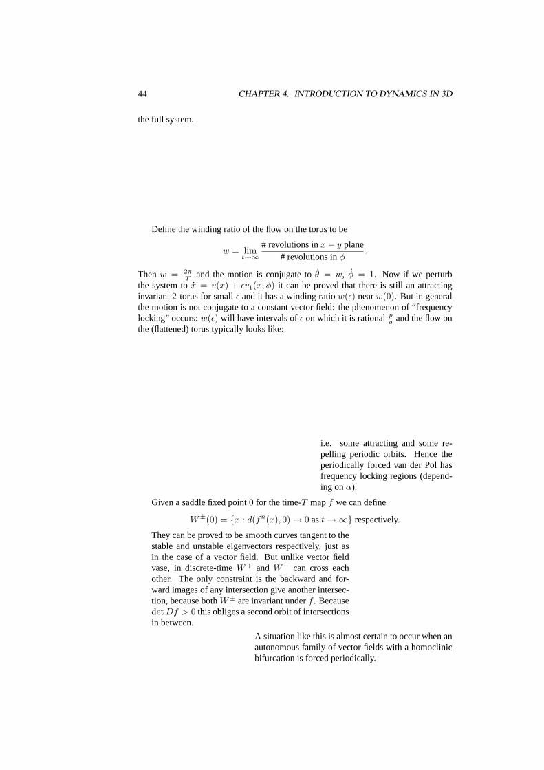
the system tox = v(x) + εv1(x, φ) it can be proved that there is still an attractinginvariant 2-torus for smallε and it has a winding ratiow(ε) nearw(0). But in generalthe motion is not conjugate to a constant vector field: the phenomenon of “frequencylocking” occurs:w(ε) will have intervals ofε on which it is rationalpq and the flow onthe (flattened) torus typically looks like:

i.e. some attracting and some re-pelling periodic orbits. Hence theperiodically forced van der Pol hasfrequency locking regions (depend-ing onα).

Given a saddle fixed point0 for the time-T mapf we can define

W±(0) = x : d(fn(x), 0) → 0 ast →∞ respectively.

They can be proved to be smooth curves tangent to thestable and unstable eigenvectors respectively, just asin the case of a vector field. But unlike vector fieldvase, in discrete-timeW+ and W− can cross eachother. The only constraint is the backward and for-ward images of any intersection give another intersec-tion, because bothW± are invariant underf . BecausedetDf > 0 this obliges a second orbit of intersectionsin between.

A situation like this is almost certain to occur when anautonomous family of vector fields with a homoclinicbifurcation is forced periodically.

4.5. DIFFERENCES FROM AUTONOMOUS SYSTEMS 45

We get these portraits.

What are the consequences of transverse homoclinic orbits? If you followW± farenough they are bound to intersect in yet another homoclinic orbit (typically two).

Obtain a boxB bounded by pieces ofW±. Now consider its forward images. Aftera finite numberN of iterations,fN (B) ∩ B consists of2 strips0 and1. Let g = fN .Then we can prove that for all sequencesa = (an)n∈Z ∈ 0, 1. There exists a pointxa ∈ B such thatgn(xa) ∈ an for all n ∈ Z, which isdeterministic chaos, behaviour


as random as a sequence of coin tosses.

References

P.A. Glendinning,Stability, Instability and Chaos, CUP, 1994.

Fairly fun to read and probably the “best” book for the course.

P.G. Drazin,Nonlinear Systems, CUP, 1992.

Again a fairly fun read but not as relevant to the course.

Guckenheimer & Holmes,Nonlinear Oscillations, Dynamical Systems and Bifurca-tions of Vector Fields, Springer, 1983.

Rather above the level of this course but probably worth a bit of bedtime reading ifyou’re interested.

Clark Robinson,Dynamical Systems, CRC Press, 1994.

Feeling brave? This one certainly isn’t bedtime reading.

Related courses

There is a course onDynamical Systemsin Part 2B.

47

Documents

Dynamics of Differential Equations