Dynamics of Consumer Demand

for New Durable Goods∗

Gautam GowrisankaranWashington University in St. Louis

and NBER

Marc RysmanDepartment of Economics

Boston University

August 28, 2007

Abstract

This paper specifies and estimates a dynamic model of consumer pref-erences for new durable goods with persistent heterogeneous consumertastes, rational expectations about future products and repeat purchasesover time. Most new consumer durable goods, particularly consumer elec-tronics, are characterized by relatively high initial prices followed by rapiddeclines in prices and improvements in quality. The evolving nature ofproduct attributes suggests the importance of modeling dynamics in es-timating consumer preferences. We estimate the model on the digitalcamcorder industry using a panel data set on prices, sales and charac-teristics. We find that dynamics are a very important determinant ofconsumer preferences and that estimated coefficients are more plausiblethan with traditional static models. We use the estimates to investigatethe value of new consumer goods and intertemporal elasticities of demand.

∗We thank Lanier Benkard, Igal Hendel, Kei Hirano, Firat Inceoglu, John Krainer, MinsooPark, Rob Porter, Jeff Prince, Pasquale Schiraldi, Andy Skrzypacz and seminar participantsat several institutions for helpful comments and Haizhen Lin, Ryan Murphy, David Rapson,Alex Shcherbakov, and Shirley Wong for research assistance. The NPD Group and ICR-CENTRIS graciously provided support in obtaining data, as did Jeff Prince and Ali Hortascu.We acknowledge funding from the National Science Foundation. All errors are our own.

1

1 Introduction

All consumers are familiar with the importance of dynamics when purchas-ing new consumer electronics technologies. A purchaser today can be sure thatwithin a short period of time, a similar product will be available for less. Rapidlyfalling prices and improving features have been one of the most visible phenom-ena in a large number of interesting and important new durable goods markets,such as computers, digital camcorders and DVD players. For instance, for digi-tal camcorders, average prices dropped from about $930 to $380 between 2000to 2006, features such as night shot diffused from 53% to 77% of models, andaverage sizes shrank significantly. A dynamic model is necessary to capture thefact that consumers choose not only what to buy but when to buy. Moreover,the rapidly evolving nature of product attributes for new durable consumergoods suggests that modeling dynamics might be empirically very important.

This paper specifies a structural dynamic model of consumer preferences fornew consumer durable goods and estimates the model using data on the digitalcamcorder industry. Accurately measuring dynamic consumer preferences fordurable goods allows for the investigation of a variety of research questions thatare of interest to both researchers and policymakers. We use the model to studythe importance of dynamics in evaluating price and characteristic elasticities,intertemporal substitution and the welfare gains from innovation for this indus-try. Our methods are also potentially applicable to other industries and otherquestions that require uncovering the dynamics of consumer preferences.1

Evaluating consumer welfare gains from new industries is necessary to de-velop price indices and understand how much innovation contributes to the econ-omy. The importance of measuring these welfare gains is underscored by thesubstantial empirical work on the welfare of new consumer durable goods. Yetmost empirical papers that examine similar industries have used static modelsof consumer demand.2 Welfare measures that are not based on dynamic modelsof demand may be biased.3 Moreover, the direction of the bias is not necessarilyclear. If consumers act as rational dynamic agents and we instead assume my-opic behavior, we may overstate the welfare gains, by assuming more high-valueconsumers than actually exist, or we may understate the welfare gains, by notrecognizing that consumers delay purchases because of the expectation of lowerprices and better features.

Our model allows for product differentiation, for persistent consumer hetero-geneity and for repeat purchases over time. Berry, Levinsohn & Pakes (1995),henceforth BLP, and the literature that follows have shown the importance of in-corporating consumer heterogeneity into differentiated product demand systemsfor obtaining realistic predictions of elasticities and welfare estimates. Much of

1For instance, Zhao (2007) extends our model to explain price reductions in the digitalcamera market and Schiraldi (2007) extends our model to study the impact of scrappingsubsidies on the second-hand automobile market.

2These include Goolsbee & Petrin (2004) for satellite cable, Ohashi (2003) for VCRs,Clements & Ohashi (2005) for video games, Chintagunta, Dube & Nair (2004) for personaldigital assistants and Einav (2007) for movie-going.

3See Aizcorbe (2005) for discussion on this point.

2

our model of consumer preferences is essentially the same as BLP: consumersin our model make a discrete choice from a set of products in a multinomiallogit model and have random coefficients over observable product character-istics. Also similar is that our model is designed for aggregate data (but canincorporate consumer-level data when available) and that prices are endogenous.

Our model departs from BLP in that products are durable and consumersare rational forward-looking agents who have the option to purchase a productin the future instead of, or in addition to, purchasing one now. Consumers donot know the future set of products, but they instead perceive a distribution forthe value of purchasing in future periods. Rather than modeling the supply sideexplicitly, we make a major simplifying assumption: that consumers perceivethat the evolution of the value of purchase will follow a simple one-dimensionalMarkov process. In this sense, consumers use a reduced-form approximationof how the supply side evolves in order to make predictions about the value offuture purchases. We assume rational expectations within the context of thissimple framework in the sense that each consumer’s expectations will be theactual empirical distribution of future product attributes.

As in most BLP-style models, our identification of key parameters such asprice elasticities and random coefficients comes from the impact of differentchoice sets on purchase probabilities using the assumption that the choice setsare exogenous. We have a tremendous amount of variation in the choice setsthat allow us to identify these parameters. Moreover, our dynamic model makesuse of substitution patterns across time periods as well as within time periodsand captures the fact that demand changes endogenously over time as consumerholdings evolve. A central limitation of this approach is that it does not allowproduct characteristics to be endogenous.

Related to our work, a recent empirical literature also seeks to estimate thepreferences for dynamic durable goods. Gandal, Kende & Rob (2000) analyzedynamic demand for homogenous products markets. Esteban & Shum (2007) es-timate a model of the second-hand automobile market with forward-looking con-sumers and firms using a simple vertical model where consumers must purchasea car every period. Prince (2007) estimates a demand model with upgradingusing disaggregate data on purchases of personal computers. Using aggregatedata on VCRs, Park (2004) interprets time dummies as capturing the value ofwaiting in a model without persistent consumer heterogeneity. More closely re-lated to our paper is Melnikov (2001), who analyzes the dynamics of consumerchoice for discrete choice differentiated products markets with durable goodsusing data on computer printers and a logit utility specification. Melnikov’sframework is similar to ours but is different in that all consumer heterogene-ity is captured by a term that is independently distributed across consumers,products and time, and in that consumers purchase only once in their lifetime.

Several recent papers generalize the Melnikov (2001) idea. Gordon (2006) es-timates the demand for computer processors, using a logit demand specificationand allowing for repeat purchases. His model does not allow for heterogene-ity across consumers or for the endogeneity of price, and allows for only fourproducts at any one time. Song & Chintagunta (2003) propose a logit utility

3

model of digital cameras that allows for random coefficients but does not allowfor the endogeneity of price and requires the number of products to stay fixedover time. Carranza (2006) also examines digital cameras, proposing a modelsimilar to ours although without repeat purchases, and suggests an alternativemethod for estimating this type of model where the dynamics are estimatedthrough a reduced-form specification that is relatively easy to estimate. Nair(2007) estimates the demand and supply for video games allowing for randomcoefficients and endogenous prices treating each video game as a monopoly.

Our paper builds on the literature on estimating dynamic demand in thatour model allows for unobserved product characteristics, repeat purchases, en-dogenous prices and multiple differentiated products and is based on an explicitdynamic model of consumer behavior. We develop new methods of inferencethat allow us to estimate this model. Our method draws on the techniquesof Berry (1994) for modeling consumer heterogeneity in a discrete choice modeland also on the Rust (1987) techniques for modeling optimal stopping decisions,where stopping corresponds to purchasing a durable good. As in Berry (1994),we solve for the vector of unobserved product characteristics for each productby finding the value of the vector that makes the predicted market share matchthe observed market share for each product. We then create a GMM estima-tor using orthogonality conditions based on the unobserved characteristics. Foreach parameter vector, Berry suggests finding the mean product characteristicsusing a contraction mapping that defines mean utilities as a function of marketshares. We use a similar process to invert the share equation. However, for aset of mean product characteristics, we explicitly evaluate the dynamic demandproblem in order to solve for the set of consumers that purchase the product ina given period. This Rust-style optimal stopping problem is nested within theBerry share inversion routine. Our methodological advance is in developing aspecification that allows us to nest these two separate methods.

The remainder of the paper is divided as follows. Section 2 discusses themodel and method of inference, Section 3 the data, Section 4 the results, andSection 5 concludes.

2 Model and Inference

In this section, we specify our dynamic model of consumer preferences, explainour method of inference and discuss the instruments and identification of theparameters.

2.1 Model

Our model starts with the introduction of a new consumer durable good attime t = 0. The unit of observation is a month and there is a continuumof heterogeneous potential consumers indexed by i. Consumers have infinitehorizons and discount the future with a common factor β. We assume thatproducts are infinitely durable. However, if a consumer who owns one product

4

purchases a new one, she obtains no additional utility from the old product, orequivalently, she discards the old product at no cost.4 We also do not considerresale markets because we believe that they are small for the new consumerdurable goods that we examine given the speed of technological progress.5

Consider the decision problem for consumer i at time t. The consumerchooses one of among Jt products in period t or chooses to purchase no productin the current period. In either case, she is faced with similar (though notidentical) decision problems at time t+1. From these Jt+1 choices, the consumerchooses the option that maximizes the sum of the expected discounted value offuture expected utilities conditional on her information at time t.

Product j at time t is characterized by observed characteristics xjt, price pjtand an unobserved (to the econometrician) characteristic ξjt. For digital cam-corders, observed characteristics include size, zoom, and the ability to take stillphotographs (among others), while the unobserved characteristic would encap-sulate product design, ergonomics and unreported recording quality. Consumerpreferences over xjt and pjt are defined respectively by the consumer-specificrandom coefficients αxi and αpi which we group together as αi. The character-istics of a product j purchased at time t, xjt and ξjt, stay constant over theinfinite life of the product. We do not model any explicit linkage between prod-ucts offered for sale at different time periods. We assume that consumers andfirms know all time t information when making their time t decisions.

Every period, each consumer obtains a flow utility based on the productthat she purchases or on the product that she already owns if she chooses notto purchase. The functional form for the flow utility fits within the randomcoefficients discrete choice framework of BLP. Specifically, we let

δfijt = αxi xjt + ξjt j = 1, . . . , Jt

denote the gross flow utility from product j purchased at time t. We assumethat a consumer purchasing product j at time t would receive a net flow utilityat time t of

uijt = δfijt − αpi ln(pjt) + εijt,

where pjt is the price of good j in period t and εijt is an idiosyncratic unob-servable meant to capture random variations in the purchase experience, suchas the sales personnel. We assume that εijt is distributed type 1 extreme value,independent across consumers, products and time, and as such has mean γ, Eu-ler’s constant. We let αi be constant over time and distributed normally withmean α ≡ (αx, αp) and variance matrix Σ, where α and Σ are parameters toestimate.6

4The model could be modified to allow for a second durable good to have value. The valueof the second good could be identified using micro data on penetration rates or individualpurchasing behavior (see Berry, Levinsohn & Pakes, 2004; Petrin, 2002).

5Schiraldi (2007) extends our model to analyze the market for used cars in Italy.6Our specification for price can be rationalized by a model where consumers consume

two products: a money good and a camcorder or outside good, and money less than onedollar generates zero utility. (Details available upon request.) The specification can easilybe modified to use the empirical income density, as in Nevo (2001)’s study on the breakfastcereal industry.

5

We also define the population mean flow utility

δfjt = αxxjt + ξjt, j = 1, . . . , Jt,

which we use to explain our method of inference in Subsection 2.2.In our model, the value of a previously purchased product is entirely captured

by its flow utility δfijt. We do not keep track of the identity of the product (forinstance, the brand). A consumer who does not purchase a new product at timet has net flow utility of

ui0t = δfi0t + εi0t,

where δfi0t is the flow utility from the product currently owned and εi0t is alsodistributed type 1 extreme value. For an individual who has purchased a productin the past, δfi0t = δf

ijt, where t is the most recent period of purchase, and j

is the product purchased at time t. Individuals who have never purchased aproduct in the past use the outside good, whose mean utility we normalize to0, so that δfi0t = 0 for those individuals.

In order to evaluate consumer i’s choice at time t, we need to formalizeconsumer i’s expectations about the utility from future products. We assumethat consumers have no information about the future values of the idiosyncraticunobservable shocks ε beyond their distribution. The set of products and theirprices and characteristics vary across time due to entry and exit and changesin prices for existing products. Consumers are uncertain about future productattributes but have rational expectations about their evolution. We assume thateach consumer is, on average over time, correct about the mean and variance ofthe future quality path.7

We now define the state variables and use them to exposit the dynamic de-cision process. Let ωt denote current product attributes xjt, pjt and ξjt forall products available at time t, and define εi.t ≡ (εi0t, . . . εiJtt). Then, thepurchase decision for consumer i depends on preferences αi and εi.t, endow-ments δfi0t, current product attributes ωt and expectations of future productattributes. Future product attributes will depend on firm behavior which is afunction of consumer endowments and supply-side factors such as technologicalprogress. Let Ωt denote current product attributes and any other factors thatinfluence future product attributes. We assume that Ωt+1 evolves according tosome Markov process P (Ωt+1|Ωt) that accounts for firm optimizing behavior.Thus, the state vector for consumer i is (εi.t, δ

fi0t,Ωt). Let V (εi.t, δ

fi0t,Ωt) de-

note the value function, and EVi(δfi0t,Ωt) =

∫εi.t

Vi(εi.t, δfi0t,Ωt)dPε denote the

expectation of the value function, integrated over realizations of εi.t. Note thatbecause εi.t is i.i.d., it satisfies the assumption of conditional independence inRust (1987).

7A more general rational expectations model would allow individual consumers to haveconsistently biased estimates of the future logit inclusive value but let the mean expectationsacross consumers be accurate. While such a model would be easy to specify, it would bedifficult to identify without expectations data.

6

We can now define the Bellman equation for consumer i as

Vi

(εi.t, δ

fi0t,Ωt

)= max

ui0t + βE

[EVi

(δfi0t,Ωt+1

)∣∣∣Ωt] , (1)

maxj=1,...,Jt

uijt + βE

[EVi

(δfijt,Ωt+1

)∣∣∣Ωt] ,where “E” denotes the expectation operator, a conditional expectation in thiscase. From (1), the consumer can choose to wait and keep her current product(option zero), or purchase any of the available products (the next Jt options).Note that the value of waiting is greater than the expected discounted stream offlow utilities ui0t + (δfi0t + γ)β/(1− β) because waiting encapsulates the optionto buy a better product in the future.

The large dimensionality of Ωt makes it very difficult to compute the Bellmanequation in (1). Thus, we proceed by making a major simplifying assumptionthat allows us to substitute a scalar variable, the logit inclusive value of purchas-ing in a given period, for Ωt in the value function. We require two definitionsto exposit the assumption. First, for each product j = 1, . . . , Jt let

δijt (Ωt) = δfijt − αpi ln (pjt) + βE

[EVi

(δfijt,Ωt+1

)∣∣∣Ωt] (2)

denote the expected discounted utility for consumer i purchasing product j attime t, integrated over εijt. Second, define the logit inclusive value for consumeri at time t to be

δit (Ωt) = ln

∑j=1,...,Jt

exp (δijt (Ωt))

. (3)

The logit assumption implies that the value of choosing from the entire set ofproducts available in period t is the same as the value of receiving one productwith mean utility δit and a single extreme value draw. In a dynamic context, aconsumer can decide whether or not to purchase this period simply by comparingδit to the outside option, accounting for expectations of future values of δit. Thecharacteristics of individual products matter only to the extent that they affectδit or expectations of its future values. Formally,

EVi

(δfi0t,Ωt

)= EVi

(δfi0t, δit, E [δit+1, δit+2, . . . |Ωt]

). (4)

Note that there is no new assumption in (4). It follows directly from the as-sumptions of the model, most directly the assumption of extreme value errors.

In this sense, we can separate the consumer’s decision problem into two parts,a choice of whether to buy, which is based on δit,∀t ≥ t, and, given purchase,the choice of what to buy, which is based on the characteristics of productsavailable at time t. This same logic has been used to simplify the choice problemfor a number of dynamic multinomial logit models (see Melnikov, 2001; Hendel& Nevo, 2007). Thus, in order to solve the consumer’s aggregate purchaseproblem, we need only to specify the distributions P (δit|Ωt) ,∀i and t > t.

7

Our main simplifying assumption is that the evolution of the logit inclusivevalue depends only on the current logit inclusive value, which we term InclusiveValue Sufficiency. Formally:

Assumption 1 Inclusive Value Sufficiency (IVS)

P (δi,t+1|Ωt) = P (δi,t+1|Ω′t) if δit (Ωt) = δit (Ω′t) .

The assumption of IVS implies that if two states have the same δit for consumeri at time t, then they result in the same distribution of future logit inclusivevalues for that consumer. As a result of IVS, we can write (with some abuse ofnotation):

EVi

(δfi0t, δit, E [δit+1, δit+2, . . . |Ωt]

)= EVi

(δfi0t, δit

). (5)

The IVS assumption is potentially restrictive. For example, δit could be higheither because there are many products in the market all with high prices orbecause there is a single product in the market with a low price. We assume thesame expectation of δi,t+1 for these two cases even though they might lead todifferent outcome in reality.8 We could lessen the restrictiveness of Assumption 1by expanding the state space beyond δit, for instance, by adding the number ofproducts as another state variable. This would not pose theoretical difficultiesbut would substantially increase computational time. In practice, we checkwhether the δit evolution is well-approximated by the simple process and itappears to be so.

The benefit of the simplifying assumption is to reduce the state space forthe decision problem of whether to purchase at time t from many dimensionsto two, as in (5). Thus, we can write the expectation Bellman equation as

EVi

(δfi0t, δit

)= ln

(exp (δit) + exp

(δfi0t + βE

[EVi

(δfi0t, δi,t+1

)∣∣∣ δit]))+ γ.

(6)We can also write the policy function, the probability that consumer i pur-chases good j, as the aggregate probability of purchase times the probability ofpurchasing a given product conditional on purchase, and then simplify:

sijt

(δfi0t, δijt, δit

)(7)

=exp (δit)

exp (δit) + exp(δfi0t + βE

[EVi

(δfi0t, δi,t+1

)∣∣∣ δit])× exp (δijt)

exp (δit)

= exp(δijt − EVi

(δfi0t, δit

)).

8A similar assumption and discussion appears in Hendel & Nevo (2007).

8

To solve the consumer decision problem, we need to specify consumer expec-tations for P (δi,t+1|δit). Consistent with our rational expectations assumption,we assume that consumer i perceives the actual empirical density of P (δi,t+1|δit)fitted to a simple functional form. Our base specification uses a simple linearautoregressive specification with drift,

δi,t+1 = γ1i + γ2iδit + uit, (8)

where uit is normally distributed with mean 0 and where γ1i and γ2i are inci-dental parameters. We estimate (8) with an easily computable linear regression,which is useful given that this regression will be performed repeatedly in ourestimation process, as noted below. It is also straightforward to extend (8) toallow a quadratic term of the form δ2

it and this would not substantially increasecomputation time.

We now briefly discuss the supply side of the model. We assume that prod-ucts arrive according to some exogenous process and that their characteristicsevolve exogenously as well. Firms have rational expectations about the futureevolution of product characteristics. After observing consumer endowments andxjt and ξjt for all current products, firms simultaneously make pricing decisions.Firms cannot commit to prices beyond the current period. These supply sideassumptions are sufficient to estimate the demand side of the model. A fullyspecified dynamic oligopoly model would be necessary to understand changesin industry equilibrium given changes in exogenous variables.

2.2 Inference

This subsection discusses the estimation of the parameters of the model, (α,Σ, β),respectively the mean consumer tastes for product characteristics and price, thevariance in consumer tastes in these variables and the discount factor. We donot attempt to estimate β because it is notoriously difficult to identify the dis-count factor for dynamic decision models (see Magnac & Thesmar, 2002). Thisis particularly true for our model, where substantial consumer waiting can beexplained by either little discounting of the future or moderate preferences forthe product. Thus, we set β = .99 at the level of the month.

We develop a method for estimating the remaining parameters that is basedon Berry (1994) and Rust (1987) and the literatures that follow.9 Our estimationalgorithm involves three levels of non-linear optimizations: on the outside is asearch over the parameters; inside that is a fixed point calculation of the vector ofpopulation mean flow utilities δfjt; and inside that is the calculation of predictedmarket shares, which is based on consumers’ dynamic optimization decisions.While both the δfjt fixed point calculation and dynamic programming estimationare well-known, our innovation is in developing a specification that allows us tonest the dynamic programming solution within the δfjt fixed point calculationto feasibly estimate the dynamics of consumer preferences.

9Computer code for performing the estimation is available from the authors upon request.

9

We now describe each of the three levels of optimization. The inner loopevaluates the vector of predicted market shares as a function of δf.. (the δfjt vec-tor) and necessary parameters by solving the consumer dynamic programmingproblem for a number of simulated consumers and then integrating across con-sumer types. Let αi ≡ (αxi , α

pi ) ∼ φl, where l is the dimensionality of αi and φl

is the standard normal density with dimensionality l. Note that αi = α+Σ1/2αiand δfijt = δfjt + Σ1/2αixjt.

For each draw, we start with initial guesses, calculate the logit inclusivevalues from (3), use these to calculate the coefficients of the product evolutionMarkov process regression in (8), and use these to calculate the expectationBellman from (6). We repeat this three-part process until convergence.Usingthe resulting policy function sijt(δ

fi0t, δijt, δit) and computed values of δijt and

δit, we then solve for market share for this draw by starting at time 0 with theassumption that all consumers hold the outside good. Iteratively for subsequenttime periods, we solve for consumer purchase decisions given the distribution offlow utility of holdings using (7) and update the distribution of flow utility ofholdings based on purchases. To perform the iterative calculation, we discretizethe state space (δfi0t, δit) and the transition matrix. We examine the impactof different numbers of grid points and different endpoints to ensure that ourapproximations are sufficient.

To aggregate across draws, a simple method would be to sample over αi andscale the draws using Σ1/2. Since our estimation algorithm is very computation-ally intensive and computational time is roughly proportional to the number ofsimulation draws, we instead use importance sampling to reduce sampling vari-ance, as in BLP. Let ssum

(αi, δ

f.., α

p,Σ)

denote the sum of predicted marketshares of any durable good at any time period for an individual with parameters(αp,Σ) and draw αi. Then, instead of sampling from the density φl we samplefrom the density

f(αi) ≡ssum

(αi, δ

f.., α

p,Σ)φl(αi)∫

ssum(α, δf.., α

p,Σ)φl(α)dα

, (9)

and then reweight draws by

wi ≡∫ssum

(α, δf.., α

p,Σ)φl(α)dα

ssum(αi, δf.., α

p,Σ) ,

in order to obtain the correct expectation. As in BLP, we sample from thedensity f by sampling from the density φl and using an acceptance/rejectioncriterion. We compute (9) using a reasonable guess of (αp,Σ) and computingδf.. from these parameters using the middle-loop procedure described below.Instead of drawing i.i.d. pseudo-random normal draws for φl, we use Haltonsequences based on the first l prime numbers to further reduce the samplingvariance (see Gentle, 2003). In practice, we use 40 draws, although results forthe base specification do not change substantively when we use 100 draws.

We now turn to the middle loop, which recovers δf.. by performing a fixedpoint equation similar to that developed by Berry (1994) and BLP. We iterate

10

until convergence

δf,newjt = δf,oldjt + ψ ·(ln(sjt)− ln

(sjt(δf,old.. , αp,Σ

))),∀j, t, (10)

where sjt(δf,old.. , αp,Σ

)is the model market share (computed in the inner loop),

sjt is actual market share, and ψ is a tuning parameter that we generally set to1 − β.10 Note that it is not necessary to treat the inner loop and middle loopas separate. We have found some computational advantages to taking a stepin (10) before the inner loop is entirely converged and to performing (6) muchmore frequently than either (8) or (3). However, we require full convergence of(3), (6), (8) and (10) before moving to the outermost loop.

The outer loop specifies a GMM criterion function

G (α,Σ) = z′ξ (α,Σ) ,

where ξ (α,Σ) is the vector of unobserved product characteristics for whichthe predicted product shares equal the observed product shares conditional onparameters, and z is a matrix of exogenous variables, described in detail inSubsection 2.3 below. We estimate parameters to satisfy(

α, Σ)

= arg minα,ΣG (α,Σ)′WG (α,Σ)

, (11)

where W is a weighting matrix.We minimize (11) by performing a nonlinear search over (αp,Σ). For each

(αp,Σ) vector, we first obtain δf.. from the middle loop. The fact that αxxjt andξjt enter flow utility linearly (recall that δfjt = αxxjt+ξjt) then allows us to solvein closed form for the αx that minimizes (11) given δf.., as in the static discretechoice literature.11 We perform the nonlinear search using a simplex method.We perform a two-stage search to obtain asymptotically efficient estimates. Inthe first stage, we let W = (z′z)−1, which would be efficient if our model werelinear instrumental variables with homoscedastic errors, and then use our firststage estimates to approximate the optimal weighting matrix.12

A simplified version of our model is one in which a given consumer is con-strained to only ever purchase one durable good. In this case, the computationof the inner loop is vastly simplified due to the fact that only consumers whohave never purchased make decisions. Because of this, (2) can be simplified toδijt = (δfijt + βγ)/(1− β)−αpi ln (pjt) which implies that δit in (3) does not de-pend on the value function. Thus, we need only solve the expectation Bellman

10One issue relates to the properties of (10). Berry provides conditions under which this

function is a contraction mapping, guaranteeing that the vector s..

(δf.., α

p,Σ, β)

is invertible

in δf... In our case, we have found examples where this inversion is not a contraction mapping,

implying that the dynamic demand system does not satisfy Berry’s conditions. Nonetheless,we have not had any problems in ensuring convergence of this process, and have not hadproblems of multiple equilibria.

11See Nevo (2000) for details. One difference from the static model is that we cannot solvein closed form for αp since the price term, αp ln (pjt) is only paid at the time of purchase,unlike ξjt.

12See again Nevo (2000) for details.

11

equation (6) for δfijt = 0 and hence there is effectively one state variable, δit,instead of two. The computation of the outer loop for this model is also quicker,since the price coefficient αp can be solved in closed-form for this model, like αx

in the base model.In practice, we compute the value function by discretizing δfi0t into 20 evenly-

spaced grid points and δit into 50 evenly-spaced grid points. We specify that δitcan take on values from 20% below the observed values to 20% above and assumethat evolutions of δit that would put it above the maximum bound simply placeit at the maximum bound. The maximum value of δit may potentially impactour results given that we examine the dynamics of a market with an improvingδit. However, we also increased the bound to 60% and found no substantivechange from the base specification, suggesting that the 20% bound is sufficient.We linearly interpolate between grid points to compute the value of any givenstate, so arguably, we approximate the value function with a linear spline ratherthan use true discretization as in Rust (1987). In solving for market shares, wediscretize δfi0t into 400 evenly spaced bins, which allows for a more accuratetracking of consumer states for this important step.

2.3 Identification and instruments

Our model follows the same identification strategy as BLP and the literaturethat follows. Heuristically, the increase in market share at product j associ-ated with a change in a characteristic of j identifies the mean of the parameterdistribution α. The Σ parameters are identified by the set of products fromwhich product j draws market share as j’s characteristics change. For instance,if product j draws only from products with similar characteristics, then thissuggests that consumers have heterogeneous valuations of characteristics whichimplies that the relevant components of Σ are large. In contrast, if j draws pro-portionally from all products, then Σ would likely be small. Because our modelis dynamic, substitution patterns across periods (in addition to within periods)identify parameters. Moreover, our model endogenously has different distribu-tions of consumer tastes for different time periods. For instance, consumers withhigh valuations for the product will likely buy early on, leaving only lower val-uation consumers in the market until such time as new features are introduced,which will draw back repeat consumers. Substitution based on this aggregatevariation in consumer tastes across time further identifies parameters.

Note that our model allows for consumers to purchase products repeatedlyover time, even though it can be estimated without any data on repeat purchaseprobabilities for individuals. At first glance, it might appear difficult to identifysuch a model. However, this model does not introduce any new parametersover the model with one-time purchases. Indeed, it does not introduce any newparameters over the static model except for the discount factor β, which wedo not estimate. The reason that it does not introduce any new parameters isthat we have made some relatively strong assumptions about the nature of theproduct: that durable goods do not wear out; that there is no resale marketfor them; and that there is no value to a household to holding more than one

12

durable good of a given type. With these assumptions, the only empiricallyrelevant reason to buy a second durable good is new features, and features areobserved in the data. While these assumptions are strong, we believe that theyare reasonable for the consumer goods that we study.

As is standard in studies of market power since Bresnahan (1981), we allowprice to be endogenous to the unobserved term (ξjt) but we assume that prod-uct characteristics are exogenous. This assumption is justified under a modelin which product characteristics are determined as part of some technologicalprogress which is exogenous to the unobserved product characteristics in anygiven period. As in Bresnahan and BLP, we do not use cost-shifters as instru-ments for price and instead exploit variables that affect the price-cost margin.Similar to BLP, we include the following variables in z: all of the product charac-teristics in x; the mean product characteristics for a given firm at the same timeperiod; the mean product characteristics for all firms at the time period; andthe count of products offered by the firm and by all firms. These variables aremeant to capture how crowded a product is in characteristic space, which shouldaffect the price-cost margin and the substitutability across products, and hencehelp identify the variance of the random coefficients and the price coefficient.While one may question the validity of these instruments, they are common inthe literature. We consider the development of alternative instruments a goodarea for future research.

3 Data

We estimate our model principally using a panel of aggregate data for digitalcamcorders.13 The data are at the monthly level and, for each model andmonth, include the number of units sold, the average price, and other observablecharacteristics. We observe 378 models and 11 brands, with observations fromMarch 2000 to May 2006. These data start from very early in the product lifecycle of digital camcorders and include the vast majority of models. The dataset was collected by NPD Techworld which surveys major electronics retailersand covers 80% of the market.14 We create market shares by dividing sales bythe number of U.S. households in a year, as reported by the U.S. Census.

We collected data on several important characteristics from on-line resources.We observe the number of pixels that the camera uses to record information,which is an important determinant of picture quality. We observe the amountof magnification in the zoom lens and the diagonal size of the LCD screen for

13We have obtained similar data for digital cameras and DVD players and previous versionsof this paper estimated models for those industries. Basic features of the results are similaracross industries. We focus on camcorders here because we believe this product exhibits theleast amount of network effects (such as titles for DVD players or complementary products forproducing pictures for digital cameras), which would complicate our analysis. Incorporatingnetwork effects into our framework is the subject of current research.

14There are major omissions from NPD’s coverage. Sales figures do not reflect on-linesellers such as Amazon and they do not cover WalMart. We do not attempt to correct forthese shortcomings.

13

Table 1: Characteristics of digital camcorders in sample Characteristic Mean Std. dev.

Continuous variables Sales 2492 (4729)

Price (Jan. 2000 $) 599 (339) Size (sq. inches width ! depth, logged) 2.69 (.542)

Pixel count (logged ÷ 10) 1.35 (.047) Zoom (magnification, logged) 2.54 (.518)

LCD screen size (inches, logged) .939 (.358) Indicator variables

Recording media: DVD .095 (.294) Recording media: tape .862 (.345)

Recording media: hard drive .015 (.120) Recording media: card (excluded) .028 (.164)

Lamp .277 (.448) Night shot .735 (.442)

Photo capable .967 (.178) Number of observations: 4436

Unit of observation: model – month

viewing shots.15 We observe the width and depth of each camera in inches(height was often unavailable), which we multiply together to create a “size”variable. We also record indicators for whether the camera has a lamp, whetherit can take still photos and whether it has “night shot” capability, an infraredtechnology for shooting in low light situations. Finally, we observe the recordingmedia the camera uses - there are four mutually exclusive media (tape, DVD,hard drive and memory card) - which we record as indicators.

To create our final data set, we exclude from the choice set in any month alldigital camcorders that sold fewer than 100 units in that month. This eliminatesabout 1% of sales from the sample. We also exclude from the choice set in anymonth all products with prices under $100 or over $2000 as these productslikely have very different usages. This eliminates a further 1.6% of sales fromthe sample. Table 1 summarizes the sales, price and characteristics data bylevel of the model-month for our final sample.

Figure 1 graphs simple averages of two features over time, size and pixelcount, using our final sample. Not surprisingly, cameras improve in these fea-tures over time. Weighting by sales produces similar results. Figure 2 displaysa similar graph for features that are characterized by indicator variables: the

15We log all continuous variables and treat any screen of less than 0.1 inch as equivalent toa screen of 0.1 inch.

14

Figure 1: Average indicator characteristics over time

1.32

1.32

1.34

1.34

1.36

1.36

1.38

1.38

Log pixel count (10s)

Log

pixe

l cou

nt (

10s)

2.4

2.4

2.6

2.6

2.8

2.8

3

3

3.2

3.2

Log size (sq in)

Log

size

(sq

in)

Jan00

Jan00

Jan02

Jan02

Jan04

Jan04

Jan06

Jan06

Log size (sq in)

Log size (sq in)

Log pixel count (10s)

Log pixel count (10s)

Figure 2: Average indicator characteristics over time

.2

.2

.4

.4

.6

.6

.8

.8

1

1

Jan00

Jan00

Jan02

Jan02

Jan04

Jan04

Jan06

Jan06

Photo capable

Photo capable

Night shot

Night shot

Lamp

Lamp

Media: tape

Media: tape

15

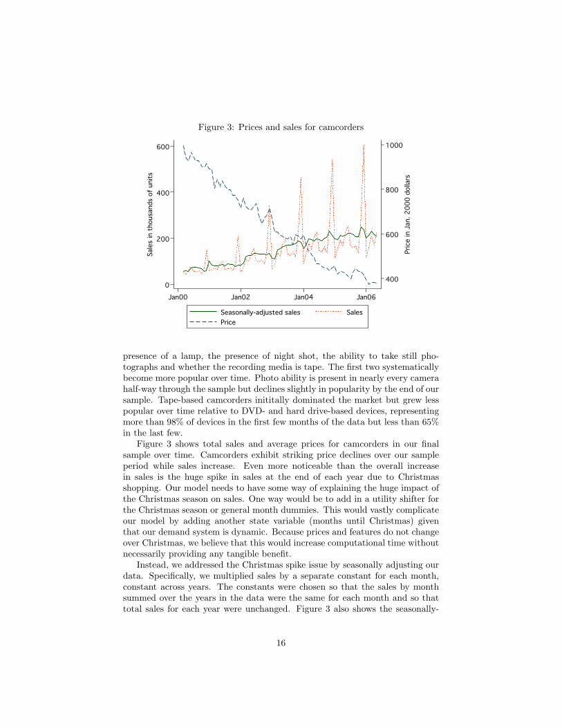
Figure 3: Prices and sales for camcorders

400

400

600

600

800

800

1000

1000

Price in Jan. 2000 dollars

Pric

e in

Jan

. 200

0 do

llars

0

0

200

200

400

400

600

600

Sales in thousands of units

Sale

s in

tho

usan

ds o

f un

its

Jan00

Jan00

Jan02

Jan02

Jan04

Jan04

Jan06

Jan06

Seasonally-adjusted sales

Seasonally-adjusted sales

Sales

Sales

Price

Price

presence of a lamp, the presence of night shot, the ability to take still pho-tographs and whether the recording media is tape. The first two systematicallybecome more popular over time. Photo ability is present in nearly every camerahalf-way through the sample but declines slightly in popularity by the end of oursample. Tape-based camcorders inititally dominated the market but grew lesspopular over time relative to DVD- and hard drive-based devices, representingmore than 98% of devices in the first few months of the data but less than 65%in the last few.

Figure 3 shows total sales and average prices for camcorders in our finalsample over time. Camcorders exhibit striking price declines over our sampleperiod while sales increase. Even more noticeable than the overall increasein sales is the huge spike in sales at the end of each year due to Christmasshopping. Our model needs to have some way of explaining the huge impact ofthe Christmas season on sales. One way would be to add in a utility shifter forthe Christmas season or general month dummies. This would vastly complicateour model by adding another state variable (months until Christmas) giventhat our demand system is dynamic. Because prices and features do not changeover Christmas, we believe that this would increase computational time withoutnecessarily providing any tangible benefit.

Instead, we addressed the Christmas spike issue by seasonally adjusting ourdata. Specifically, we multiplied sales by a separate constant for each month,constant across years. The constants were chosen so that the sales by monthsummed over the years in the data were the same for each month and so thattotal sales for each year were unchanged. Figure 3 also shows the seasonally-

16

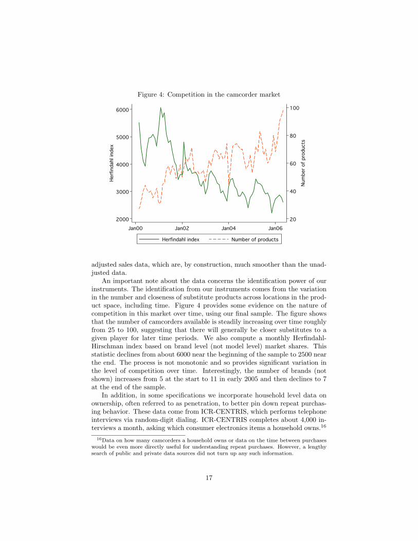
Figure 4: Competition in the camcorder market

20

20

40

40

60

60

80

80

100

100

Number of products

Num

ber

of p

rodu

cts

2000

2000

3000

3000

4000

4000

5000

5000

6000

6000

Herfindahl index

Herf

inda

hl in

dex

Jan00

Jan00

Jan02

Jan02

Jan04

Jan04

Jan06

Jan06

Herfindahl index

Herfindahl index

Number of products

Number of products

adjusted sales data, which are, by construction, much smoother than the unad-justed data.

An important note about the data concerns the identification power of ourinstruments. The identification from our instruments comes from the variationin the number and closeness of substitute products across locations in the prod-uct space, including time. Figure 4 provides some evidence on the nature ofcompetition in this market over time, using our final sample. The figure showsthat the number of camcorders available is steadily increasing over time roughlyfrom 25 to 100, suggesting that there will generally be closer substitutes to agiven player for later time periods. We also compute a monthly Herfindahl-Hirschman index based on brand level (not model level) market shares. Thisstatistic declines from about 6000 near the beginning of the sample to 2500 nearthe end. The process is not monotonic and so provides significant variation inthe level of competition over time. Interestingly, the number of brands (notshown) increases from 5 at the start to 11 in early 2005 and then declines to 7at the end of the sample.

In addition, in some specifications we incorporate household level data onownership, often referred to as penetration, to better pin down repeat purchas-ing behavior. These data come from ICR-CENTRIS, which performs telephoneinterviews via random-digit dialing. ICR-CENTRIS completes about 4,000 in-terviews a month, asking which consumer electronics items a household owns.16

16Data on how many camcorders a household owns or data on the time between purchaseswould be even more directly useful for understanding repeat purchases. However, a lengthysearch of public and private data sources did not turn up any such information.

17

Figure 5: Penetration and sales of digital camcorders

0

0

.05

.05

.1

.1

.15

.15

Fraction of U.S. households

Frac

tion

of U

.S. h

ouse

hold

s

2000q3

2000q3

2001q3

2001q3

2002q3

2002q3

2003q3

2003q3

2004q3

2004q3

2005q3

2005q3

2006q3

2006q3

Penetration (ICR-CENTRIS)

Penetration (ICR-CENTRIS)

New sales (NPD)

New sales (NPD)

New penetration (ICR-CENTRIS)

New penetration (ICR-CENTRIS)

Figure 5 shows our ICR-CENTRIS data, which contain the percent of house-holds that indicate holding a digital camcorder in the third quarter of the yearfor 1999 to 2006. It also shows the year-to-year change in this number and thenew sales of camcorders, as reported by NPD.

The penetration data show rapid growth in penetration early on in the sam-ple but no growth by the end. The evidence from the penetration and sales dataare not entirely consistent, perhaps due to differences in sampling methodology:in 3 of the 6 years, the increase in penetration is larger than the increase innew sales. We also believe the ICR-CENTRIS finding of virtually no new pene-tration after 2004 to be implausible. Nonetheless, the slowdown in penetrationbut continued growth in sales together suggest that there are substantial repeatpurchases by the end of our sample. Because of the issues surrounding the pen-etration data, we only use it in one robustness specification, as we discuss inSection 4.2 below.

4 Results and implications

We first exposit our results, then provide evidence on the fit of the model, andfinally discuss the implications of the results.

4.1 Results

We present our parameter estimates in Table 2. Table 2 contains six columnsof results. The first column of results provides the parameter estimates and

18

Table 2: Parameter estimates

Parameter

Base dynam

ic m

odel

Dynam

ic m

odel with

extra random

coefficients

Dynam

ic m

odel without

repurchases Static m

odel Static m

odel aggregated to

year

Dynam

ic m

odel with

micro

mom

ents M

ean coefficients (α)

Constant –.141 (.044) *

–.097 (.195) * –.087 (1.5)

–8.90 (2e3) –4.03 (132)

–.243 (.213) Log price

–2.66 (.576) * –2.74 (.975) *

–.056 (72.6) .0247 (19.1)

–.089 (14.5) –3.01 (.582) *

Log size –.007 (.001) *

–.007 (.014) –.002 (7e-4) *

–.152 (.068) –.340 (.204)

–.019 (.002) * Log pixel

.095 (.050) .098 (.028) *

–.002 (.027) –2.56 (2.43)

–4.52 (5.85) .241 (.146) *

Log zoom

.007 (.002) * .007 (.002) *

.007 (9e-4) * .654 (.086) *

.861 (.269) .010 (.004) *

Log LCD size

.003 (.001) * .003 (.001) *

–5e-4 (9e-4) –.053 (.105)

–.361 (.325) .011 (.004) *

Media: D

VD

.025 (.005) *

.027 (.006) * –.001 (.004)

–.177 (.344) .229 (1.35)

.052 (.017) * M

edia: tape .007 (.005)

.007 (.005) –.007 (.003) *

–.763 (.333) * –.671 (1.05)

.017 (.016) M

edia: HD

.020 (.006)

.023 (.008) * –.008 (.004)

–.873 (.425) * –1.32 (1.59)

.039 (.019) * Lam

p .006 (.001) *

.007 (.001) * –.002 (.001)

–.209 (.130) –.351 (.402)

.002 (.004) N

ight shot .009 (.001) *

.009 (.001) * .007 (6e-4) *

.646 (.073) * 1.20(.199)

.022 (.003) * Photo capable

–.014 (.002) * –.015 (.003) *

–.005 (.002) * –.431 (.205) *

–.432 (.767) –.022 (.007) *

Standard deviation coefficients (Σ1/2)

Constant

.086 (.025) * .058 (.130)

2e-5 (27) .007 (4e4)

.036 (1e3) 1e-7 (.082)

Log price 7e-6 (.563)

.043 (8.06) .0002 (817)

.001 (267) .011 (67.7)

.651 (.233) * Log size

5e-09 (.096)

Log pixel

.0015 (.337)

Standard errors in parentheses; statistical significance at 5%

level indicated with *

19

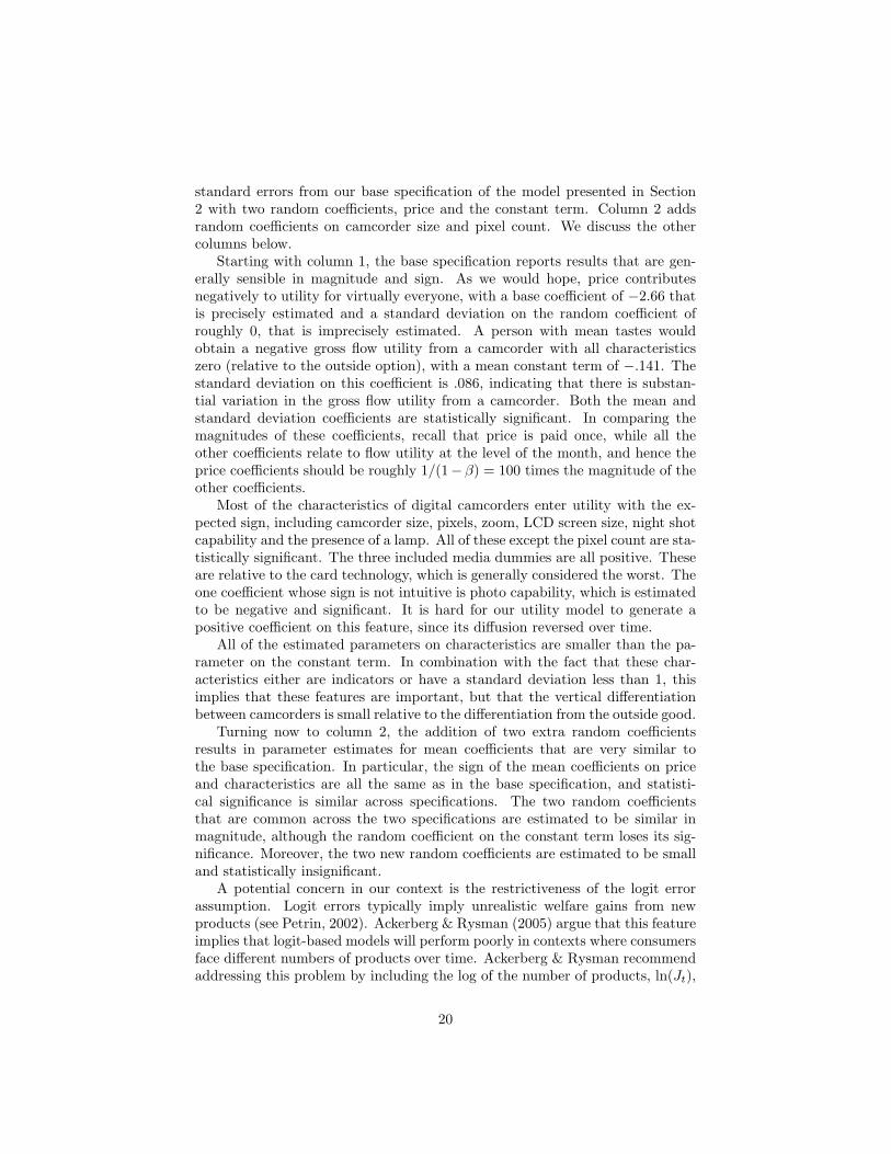
standard errors from our base specification of the model presented in Section2 with two random coefficients, price and the constant term. Column 2 addsrandom coefficients on camcorder size and pixel count. We discuss the othercolumns below.

Starting with column 1, the base specification reports results that are gen-erally sensible in magnitude and sign. As we would hope, price contributesnegatively to utility for virtually everyone, with a base coefficient of −2.66 thatis precisely estimated and a standard deviation on the random coefficient ofroughly 0, that is imprecisely estimated. A person with mean tastes wouldobtain a negative gross flow utility from a camcorder with all characteristicszero (relative to the outside option), with a mean constant term of −.141. Thestandard deviation on this coefficient is .086, indicating that there is substan-tial variation in the gross flow utility from a camcorder. Both the mean andstandard deviation coefficients are statistically significant. In comparing themagnitudes of these coefficients, recall that price is paid once, while all theother coefficients relate to flow utility at the level of the month, and hence theprice coefficients should be roughly 1/(1− β) = 100 times the magnitude of theother coefficients.

Most of the characteristics of digital camcorders enter utility with the ex-pected sign, including camcorder size, pixels, zoom, LCD screen size, night shotcapability and the presence of a lamp. All of these except the pixel count are sta-tistically significant. The three included media dummies are all positive. Theseare relative to the card technology, which is generally considered the worst. Theone coefficient whose sign is not intuitive is photo capability, which is estimatedto be negative and significant. It is hard for our utility model to generate apositive coefficient on this feature, since its diffusion reversed over time.

All of the estimated parameters on characteristics are smaller than the pa-rameter on the constant term. In combination with the fact that these char-acteristics either are indicators or have a standard deviation less than 1, thisimplies that these features are important, but that the vertical differentiationbetween camcorders is small relative to the differentiation from the outside good.

Turning now to column 2, the addition of two extra random coefficientsresults in parameter estimates for mean coefficients that are very similar tothe base specification. In particular, the sign of the mean coefficients on priceand characteristics are all the same as in the base specification, and statisti-cal significance is similar across specifications. The two random coefficientsthat are common across the two specifications are estimated to be similar inmagnitude, although the random coefficient on the constant term loses its sig-nificance. Moreover, the two new random coefficients are estimated to be smalland statistically insignificant.

A potential concern in our context is the restrictiveness of the logit errorassumption. Logit errors typically imply unrealistic welfare gains from newproducts (see Petrin, 2002). Ackerberg & Rysman (2005) argue that this featureimplies that logit-based models will perform poorly in contexts where consumersface different numbers of products over time. Ackerberg & Rysman recommendaddressing this problem by including the log of the number of products, ln(Jt),

20

as a regressor, as if it were a linear element in δfjt. Finding a coefficient of0 implies the logit model is well-specified, whereas a coefficient of -1 implies“full-crowding,” that consumers respond to increases in the number of productsas if there are no new logit draws. In unreported results, we find that otherparameters change little and that the coefficient on ln(Jt) is -0.015. Althoughthe coefficient is statistically significant, it is very close to zero and suggeststhat the i.i.d. logit draws are a reasonable approximation. Concerns with theimplications of logit draws motivate Berry & Pakes (2005) and Bajari & Benkard(2005) to propose discrete choice models that do not include logit i.i.d. errorterms, but given this coefficient estimate, we do not further pursue this issue.

Column 3 provides estimates from the dynamic model where individuals arerestricted to purchase at most one digital camcorder ever. This specificationyields results that are less appealing than our base specification. In particular,the mean price coefficient drops in magnitude by a factor of 5 and loses itsstatistical significance. Many of the characteristics enter mean utility with anunexpected sign, including pixels, LCD screen size and lamp and many fewermean coefficients are significant than in the base specification. The standarddeviation coefficients are very small and statistically insignificant.

It is useful to understand why the model with multiple purchases provides amuch larger price coefficient than the dynamic model with purchases restrictedto one-time only. In the one-time purchase model, the magnitude of the meanprice coefficient is much smaller than the standard deviation of the extreme valuedistribution. Had this estimated coefficient been applied to the base model, theδfijt values would have to be sufficiently negative to prevent individuals frompurchasing a product most months, implying that individuals dislike havingtheir purchased camcorder. In addition to being intuitively unappealing, thenegative δfijt values resulted in a very bad fit of the moment criteria for thebase model. Thus, the multiple purchase feature of the base model essentiallyforces the price coefficient to be sufficiently negative to avoid implications thatare counterintuitive and also do not fit the data well.

Column 4 essentially follows BLP and estimates a traditional static randomcoefficients discrete choice specification. To compare these coefficients with thebase specification, one would have to multiply all the coefficients from this spec-ification, except for the coefficients on price, by 1/100. The static model yieldsmany unappealing results, including a positive mean price coefficient and manycoefficients on characteristics that are of the opposite sign from expected. Col-umn 5 estimates a variant of the static model where we aggregate the productsto the annual level.17 The results from this specification are similar to theresults from column 4.

We believe that the very imprecise and sometimes positive price coefficientsin the static specifications is caused by the fact that the data cannot easily beexplained by a static model. In particular, the static model cannot fit two factsthat are characteristic of the data: first, many more people purchased digital

17This specification drops the first and last year from our data, as we lack information onall months for those years.

21

camcorders once prices fell; but second, within a time period, the cheapest mod-els were often not the most popular. Because the model cannot then estimatea significantly negative price coefficient, it also does not result in appropriatecoefficients on characteristics.

The dynamic model addresses these two facts because it predicts that peoplewait to purchase because of the expectations of price declines and not directlybecause of high prices. Heuristically, the static price coefficient is analogousto the coefficient from a regression of market shares on prices whereas the thedynamic price coefficient is analogous to the coefficient from a regression ofshares on the forward difference in price, (pjt − βpjt+1).18 Unlike the staticexplanation, the dynamic explanation for why consumers wait does not conflictwith consumers buying relatively high-priced products.

4.2 Fit of the model

We first assess the fit of the model, by reporting the simple average of theunobserved quality ξjt for each month in Figure 6. For this figure and all thatfollow, we use the estimated parameters reported in the first column of Table 2and the vector of δxjt that are consistent with these parameters and with observedshares. Note that ξjt is the estimation error of the model. The figure does notindicate any systematic autocorrelation or heteroscedasticity of the average errorover time. This finding is important because there is no reduced-form featuresuch as a time trend to match the diffusion path. If one were to match, forinstance, an S-shaped diffusion path with a simple linear regression, we wouldexpect to have systematically correlation in ξjt. However, Figure 6 does notindicate any such pattern.

We next examine the reasonableness of the IVS assumption. Our estimatesof the dynamic models of consumer preferences rely on the IVS assumption, thatconsumers perceive that next month’s logit inclusive value δi,t+1 depends onlyon the current logit inclusive value δit and only within a simple autoregressivespecification with drift. Figure 7 plots δit for 3 sets of random coefficients at theestimated parameter values: individuals with random coefficients that result inthem being in the 20th, 50th and 80th percentile of δit in the median month ofthe sample.

One can see that there is a general upward trend in these values throughoutour sample period. Moreover, the trend looks roughly linear. Consistent withTable 2, Figure 7 shows that there are significant differences in valuations acrosscoefficients. By the end of the sample period, the value of purchasing a cam-corder for a 20th percentile individual is still less than the value for a medianindividual at the beginning of the sample period. This is consistent with thefact that total digital camcorder sales by the end of our period were only about10% of the size of the number of U.S. households. The three paths of coeffi-cients move in parallel, rising and dipping in the same months in response to

18Gandal et al. (2000) show that this heuristic is an exact description of the market withone product, perfect foresight, zero variance to εijt, linearity in prices, no repeat purchase,and a concave price path.

22

Figure 6: Average estimation error (ξjt) by month

-.01

-.01

-.005

-.005

0

0

.005

.005

.01

.01

Jan00

Jan00

Jan02

Jan02

Jan04

Jan04

Jan06

Jan06

Mean xsi

Mean xsi

Zero base

Zero base

Figure 7: Evolution of δit over time

-25

-25

-20

-20

-15

-15

-10

-10

-5

-5

Jan00

Jan00

Jan02

Jan02

Jan04

Jan04

Jan06

Jan06

delta_it 20th percentile

delta_it 20th percentile

delta_it 50th percentile

delta_it 50th percentile

delta_it 80th percentile

delta_it 80th percentile

23

Figure 8: Difference between δit+1 and its period t prediction

-.5

-.5

0

0

.5

.5

1

1

Jan00

Jan00

Jan02

Jan02

Jan04

Jan04

Jan06

Jan06

Mean consumer prediction error

Mean consumer prediction error

Zero base

Zero base

the introduction of new products and features and pricing changes. This is notsurprising as the underlying results show that almost all of the heterogeneity isassociated with the constant term rather than the valuation of prices.

Figure 7 suggests that the IVS assumption is reasonable. Of course, theresults of this figure are based on values evaluated at the structural parameters,and so we cannot rule out the possibility that a more general industry evolutionassumption would have resulted in different structural parameters that thenwould have generated a different pattern of evolution.

Another way of evaluating the industry evolution assumption is to examinethe prediction error from the consumer decision problem. In Figure 8 we evalu-ate the mean value across random coefficients of the prediction error, which isδi,t+1 − (γ1i + γ2iδit), where γ1i and γ2i are the estimated parameters from theregression specified in (8). The figure shows that the prediction errors fluctuaterapidly from negative to positive. There is not an overall trend where they arebecoming more positive or more negative over time. In contrast, the resultsshow that, consistent with our model, short-run changes in product attributesare the source of the difference between consumers’ predictions of future valuesand their actual values. This provides further evidence that the evolution pro-cess that we specify is reasonable. However, Figure 8 does appear to show thatthe variance of the prediction errors decreases somewhat over time, althoughour model imposes that the variance of the residual is constant over time.

We obtain a final measure of the fit of the model by examining the extentto which we observe repeat purchasing behavior in our sample. Figure 9 plotsthe fraction of shares due to repeat purchases for the base model as well as

24

Figure 9: Evolution of repeat purchase sales

0

0

.05

.05

.1

.1

.15

.15

.2

.2

.25

.25

Fraction of sales from repeat purchasers

Frac

tion

of s

ales

fro

m r

epea

t pu

rcha

sers

Jan00

Jan00

Jan02

Jan02

Jan04

Jan04

Jan06

Jan06

Base model

Base model

Model with additional moment

Model with additional moment

for a robustness specification that we discuss below. Under the base model,repeat purchases account for a very small fraction of total sales. Even in thefinal period, which has the largest fraction, repeat purchases account for onlyabout .25% of new sales. The underlying reason why there are not more repeatpurchases is that the coefficients on characteristics other than the constant termare small relative to the utility contribution from the price and the constantterms, implying that the net benefit to upgrading is low.

This finding is not consistent with the evidence, albeit imperfect, from theICR-CENTRIS household penetration survey, that new sales are higher thannew penetration. Thus, we use the penetration data in the form of a micro-moment (see Petrin, 2002) as a robustness check on our base results. Specifically,we use the penetration data to construct an additional moment that is thedifference between the increase in household penetration between September2002 and September 2005 predicted by the model and by the penetration data.19

We chose to use only these two years to mitigate the noise present in the data.Table 2 column 6 presents results from this specification with an additional

moment. The coefficient estimates on characteristics are similar to the basespecification although generally somewhat larger. More importantly, the stan-dard deviation of the random coefficient on price goes from being roughly 0 tobeing relatively large (more than one fifth the size of the mean price coefficient)and statistically significant, while the standard deviation of the random coeffi-cient on the constant term changes in the opposite direction, to being roughly

19See Berry et al. (2004) and Petrin (2002) for details on calculating weighting matriceswhen combining micro moments with aggregate moments.

25

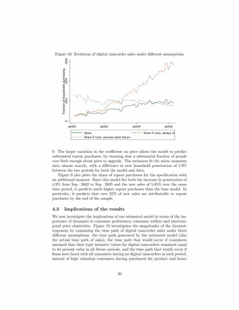
Figure 10: Evolution of digital camcorder sales under different assumptions

0

0

.002

.002

.004

.004

.006

.006

Fraction of households purchasing

Frac

tion

of h

ouse

hold

s pu

rcha

sing

Jan00

Jan00

Jan02

Jan02

Jan04

Jan04

Jan06

Jan06

Share

Share

Share if cons. always in

Share if cons. always in

Share if cons. assume same future

Share if cons. assume same future

0. The larger variation in the coefficient on price allows the model to predictsubstantial repeat purchases, by ensuring that a substantial fraction of peoplecare little enough about price to upgrade. The estimates fit the micro momentsdata almost exactly, with a difference in new household penetration of 4.9%between the two periods for both the model and data.

Figure 9 also plots the share of repeat purchases for the specification withan additional moment. Since this model fits both the increase in penetration of4.9% from Sep. 2002 to Sep. 2005 and the new sales of 5.85% over the sametime period, it predicts much higher repeat purchases than the base model. Inparticular, it predicts that over 25% of new sales are attributable to repeatpurchases by the end of the sample.

4.3 Implications of the results

We now investigate the implications of our estimated model in terms of the im-portance of dynamics in consumer preferences, consumer welfare and intertem-poral price elasticities. Figure 10 investigates the magnitudes of the dynamicresponses by examining the time path of digital camcorder sales under threedifferent assumptions: the time path generated by the estimated model (alsothe actual time path of sales), the time path that would occur if consumersassumed that their logit inclusive values for digital camcorders remained equalto its present value in all future periods, and the time path that would occur iffirms were faced with all consumers having no digital camcorders in each period,instead of high valuation consumers having purchased the product and hence

26

Figure 11: Mean per-capita consumer surplus from digital camcorder industry

120

120

140

140

160

160

180

180

200

200

Year 2000 dollars

Year

200

0 do

llars

Jan00

Jan00

Jan02

Jan02

Jan04

Jan04

Jan06

Jan06

Mean value of industry

Mean value of industry

Mean value with const. price

Mean value with const. price

generally having a higher reservation utility for buying, as occurs in our model.All results in this subsection use the parameter estimates from our base modelin Table 2 column 1.

We find that dynamics explain a very important part of the sales path.In particular, if consumers did not assume that prices and qualities changed,then sales would be somewhat declining over time, instead of growing rapidlyover the sample period. At the beginning of our sample period, sales would behuge compared to actual sales, as many consumers would have perceived only alimited option value from waiting. By the end of our sample period, sales wouldbe significantly less than current sales, as many consumers who were likely tobuy digital camcorders would have bought them early on, having assumed thatquality, in the sense of the logit inclusive value, would be stable over time.

If firms were faced with a situation where all consumers had only the outsidegood in every period, then the sales path would be similar until roughly twoyears into our sample. At this point, many of the high valuation consumers hadstarted to purchase. By the end of our sample period, we find that sales in thefinal month would have been about 3 times as high as they actually were. Notethat this increase in sales is due to high valuation consumers not owning anydigital camcorders, and mostly not to having a larger market, as roughly 90% ofthe market had not purchased any digital camcorder by the end of our sampleperiod.

Figure 11 examines the extent to which the digital camcorder industry hascreated consumer surplus. This provides evidence on the welfare gains from thisnew goods industry. We evaluate the expected discounted consumer surplus at

27

Figure 12: Industry dynamic price elasticities

-2

-2

-1.5

-1.5

-1

-1

-.5

-.5

0

0

Percent quantity change from baseline

Perc

ent

quan

tity

chan

ge f

rom

bas

elin

e

-5

-5

0

0

5

5

10

10

15

15

Months after price change

Months after price change

Permanent price change

Permanent price change

Temp. price change

Temp. price change

Temp. price change believed permanent

Temp. price change believed permanent

Zero base

Zero base

each period by integrating the welfare across consumer random coefficients forthe δit of that period and consumer type. We evaluate the value of the industryfor each consumer at each point in time using as the basis point a world where noone owns a digital camcorder. For each consumer random coefficient, we obtainthe welfare by dividing the value (measured in utility units) by the marginalutility of a dollar, which we calculate using a price of $525, which is the sales-weighted mean price of a digital camcorder in our sample.

Our results reveal that the digital camcorder market has contributed anaverage of $125 in expected discounted consumer surplus per U.S. householdfrom the point of view of 2000, or an average of $1.25 per month. The valueof the industry rises to about $200 by 2006. Note that the rise is less than theincrease in value of the industry characteristics across these time periods, sincethe value in 2000 incorporates the fact that the industry will improve over time.

Figure 11 also plots the change in valuation over time with the assumptionthat prices for all products are equal to the weighted mean price of $525. Thisplot shows that roughly half of the value gain between the start and end of oursample is due to the reduction in price. The other half is due to improvementsin characteristics and increases in the number of available products.

It would be of use to compare this number to the comparable figure fromthe static estimation of the digital camcorder industry. However, the staticestimation would provide a negative valuation number since the price coefficientis estimated to be positive. Since a negative number is clearly not plausible, wedid not report the number for the static estimation.

Finally, we analyze intertemporal price elasticities. To evaluate the impor-

28

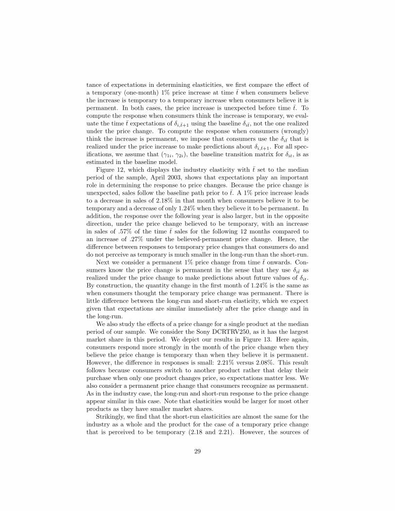
tance of expectations in determining elasticities, we first compare the effect ofa temporary (one-month) 1% price increase at time t when consumers believethe increase is temporary to a temporary increase when consumers believe it ispermanent. In both cases, the price increase is unexpected before time t. Tocompute the response when consumers think the increase is temporary, we eval-uate the time t expectations of δi,t+1 using the baseline δit, not the one realizedunder the price change. To compute the response when consumers (wrongly)think the increase is permanent, we impose that consumers use the δit that isrealized under the price increase to make predictions about δi,t+1. For all spec-ifications, we assume that (γ1i, γ2i), the baseline transition matrix for δit, is asestimated in the baseline model.

Figure 12, which displays the industry elasticity with t set to the medianperiod of the sample, April 2003, shows that expectations play an importantrole in determining the response to price changes. Because the price change isunexpected, sales follow the baseline path prior to t. A 1% price increase leadsto a decrease in sales of 2.18% in that month when consumers believe it to betemporary and a decrease of only 1.24% when they believe it to be permanent. Inaddition, the response over the following year is also larger, but in the oppositedirection, under the price change believed to be temporary, with an increasein sales of .57% of the time t sales for the following 12 months compared toan increase of .27% under the believed-permanent price change. Hence, thedifference between responses to temporary price changes that consumers do anddo not perceive as temporary is much smaller in the long-run than the short-run.

Next we consider a permanent 1% price change from time t onwards. Con-sumers know the price change is permanent in the sense that they use δit asrealized under the price change to make predictions about future values of δit.By construction, the quantity change in the first month of 1.24% is the same aswhen consumers thought the temporary price change was permanent. There islittle difference between the long-run and short-run elasticity, which we expectgiven that expectations are similar immediately after the price change and inthe long-run.

We also study the effects of a price change for a single product at the medianperiod of our sample. We consider the Sony DCRTRV250, as it has the largestmarket share in this period. We depict our results in Figure 13. Here again,consumers respond more strongly in the month of the price change when theybelieve the price change is temporary than when they believe it is permanent.However, the difference in responses is small: 2.21% versus 2.08%. This resultfollows because consumers switch to another product rather that delay theirpurchase when only one product changes price, so expectations matter less. Wealso consider a permanent price change that consumers recognize as permanent.As in the industry case, the long-run and short-run response to the price changeappear similar in this case. Note that elasticities would be larger for most otherproducts as they have smaller market shares.

Strikingly, we find that the short-run elasticities are almost the same for theindustry as a whole and the product for the case of a temporary price changethat is perceived to be temporary (2.18 and 2.21). However, the sources of

29

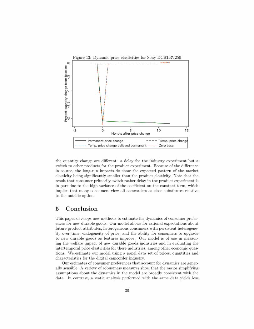
Figure 13: Dynamic price elasticities for Sony DCRTRV250

-2

-2

-1.5

-1.5

-1

-1

-.5

-.5

0

0

Percent quantity change from baseline

Perc

ent

quan

tity

chan

ge f

rom

bas

elin

e

-5

-5

0

0

5

5

10

10

15

15

Months after price change

Months after price change

Permanent price change

Permanent price change

Temp. price change

Temp. price change

Temp. price change believed permanent

Temp. price change believed permanent

Zero base

Zero base

the quantity change are different: a delay for the industry experiment but aswitch to other products for the product experiment. Because of the differencein source, the long-run impacts do show the expected pattern of the marketelasticity being significantly smaller than the product elasticity. Note that theresult that consumer primarily switch rather delay in the product experiment isin part due to the high variance of the coefficient on the constant term, whichimplies that many consumers view all camcorders as close substitutes relativeto the outside option.

5 Conclusion

This paper develops new methods to estimate the dynamics of consumer prefer-ences for new durable goods. Our model allows for rational expectations aboutfuture product attributes, heterogeneous consumers with persistent heterogene-ity over time, endogeneity of price, and the ability for consumers to upgradeto new durable goods as features improve. Our model is of use in measur-ing the welfare impact of new durable goods industries and in evaluating theintertemporal price elasticities for these industries, among other economic ques-tions. We estimate our model using a panel data set of prices, quantities andcharacteristics for the digital camcorder industry.

Our estimates of consumer preferences that account for dynamics are gener-ally sensible. A variety of robustness measures show that the major simplifyingassumptions about the dynamics in the model are broadly consistent with thedata. In contrast, a static analysis performed with the same data yields less

30

realistic results.We find substantial heterogeneity in the overall utility from digital cam-

corders. Our results also show that much of the reason why the initial marketshare for digital camcorders was not higher was because consumers were ratio-nally expecting that the market would later yield cheaper and better players.We find that industry elasticity of demand is 2.18 for transitory price shocksand 1.24 for permanent price shocks, with significantly larger elasticities for in-dividual products. Last, we find that the digital camcorder industry is worthan average of $125 in expected value at the start of the industry.

We believe that our results show that dynamic estimation of consumer pref-erences is both feasible and important for analyzing industries with new goods.We see several avenues of future research, including evaluating firm decisionproblems in the presence of consumer and firm dynamics.

31

References

Ackerberg, D. A. & Rysman, M. (2005). Unobservable product differentiation indiscrete choice models: Estimating price elasticities and welfare effects. RANDJournal of Economics, 36, 771–788.

Aizcorbe, A. (2005). Price deflators for high technology goods and the new buyerproblem. Unpublished manuscript, Board of Governors of the Federal Reserve Bank.

Bajari, P. & Benkard, C. L. (2005). Demand estimation with heterogeneous consumersand unobserved product characteristics: A hedonic approach. Journal of PoliticalEconomy, 113, 1239–1276.

Berry, S. (1994). Estimating discrete choice models of product differentiation. RANDJournal of Economics, 25, 242–262.

Berry, S., Levinsohn, J., & Pakes, A. (1995). Automobile prices in market equilibrium.Econometrica, 63, 841–890.

Berry, S., Levinsohn, J., & Pakes, A. (2004). Estimating differentiated product demandsystems from a combination of micro and macro data: The market for new vehicles.Journal of Political Economy, 112, 68–105.

Berry, S. & Pakes, A. (2005). The pure characteristics model of demand. InternationalEconomic Review, in press.

Bresnahan, T. F. (1981). Departures from marginal cost pricing in the americanautomobile industry: Estimates for 1997-1978. Journal of Industrial Economics,17, 201–277.

Carranza, J. (2006). Demand for durable goods and the dynamics of quality. Unpub-lished manuscript, University of Wisconsin.

Chintagunta, P., Dube, J., & Nair, H. (2004). Empirical analysis of indirect networkeffects in the market for personal digital assistants. Quantitative Marketing andEconomics, 2 (1), 23–58.

Clements, M. & Ohashi, H. (2005). Indirect network effects and the product cycle:Video games in the U.S., 1994-2002. Journal of Industrial Economics, 53, 515–542.

Einav, L. (2007). Seasonality in the U.S. motion picture industry. RAND Journal ofEconomics, 38, in press.

Esteban, S. & Shum, M. (2007). Durable goods oligopoly with secondary markets:The case of automobiles. RAND Journal of Economics, in press.

Gandal, N., Kende, M., & Rob, R. (2000). The dynamics of technological adoption inhardware/software systems: The case of compact disc players. RAND Journal ofEconomics, 31, 43–61.

Gentle, J. E. (2003). Random number generation and Monte Carlo methods (2 ed.).New York: Springer.

Goolsbee, A. & Petrin, A. (2004). The consumer gains from direct broadcast satellitesand the competition with cable television. Econometrica, 72, 351–381.

32

Gordon, B. (2006). Estimating a dynamic model of demand for durable goods. Un-published manuscript, Carnegie Mellon University.

Hendel, I. & Nevo, A. (2007). Measuring the implications of sales and consumerstockpiling behavior. Econometrica, in press.

Magnac, T. & Thesmar, D. (2002). Identifying dynamic discrete decision processes.Econometrica, 70, 801–816.

Melnikov, O. (2001). Demand for differentiated products: The case of the U.S. com-puter printer market. Unpublished manuscript, Cornell University.

Nair, H. (2007). Intertemporal price discrimination with forward-looking consumers:Application to the US market for console video games. Quantitative Marketing andEconomics, in press.

Nevo, A. (2000). A practitioner’s guide to estimation of random coefficients logitmodels of demand. Journal of Economics & Management Strategy, 9, 513–548.

Nevo, A. (2001). Measuring market power in the ready-to-eat breakfast cereal industry.Econometrica, 69, 307–342.

Ohashi, H. (2003). The role of network effects in the U.S. VCR market, 1978-86.Journal of Economics and Management Strategy, 12, 447–494.

Park, S. (2004). Quantitative analysis of network externalities in competing technolo-gies: The VCR case. Review of Economics and Statistics, 86, 937–945.

Petrin, A. (2002). Quantifying the benefits of new products: The case of the minivan.Journal of Political Economy, 110, 705–729.

Prince, J. (2007). Repeat purchase amid rapid quality improvement: Structural esti-mation of demand for personal computers. Unpublished manuscript, Cornell Uni-versity.

Rust, J. (1987). Optimal replacement of GMC bus engines: An empirical model ofHarold Zurcher. Econometrica, 55, 999–1033.

Schiraldi, P. (2007). Autobmobile replacement: A dynamic structural approach. Un-published Manuscript, Boston University.

Song, I. & Chintagunta, P. (2003). A micromodel of new product adoption withheterogeneous and forward-looking consumers: An application to the digital cameracategory. Quantitative Marketing and Economics, 1, 371–407.

Zhao, Y. (2007). Why are prices falling fast? An empirical study of the US digitalcamera market. Unpublished Manuscript, Yale University.

33