Embed Size (px)
Citation preview

Preprint typeset in JHEP style - HYPER VERSION Lent Term, 2013
Dynamics and RelativityUniversity of Cambridge Part IA Mathematical Tripos
David Tong
Department of Applied Mathematics and Theoretical Physics,
Centre for Mathematical Sciences,
Wilberforce Road,
Cambridge, CB3 OBA, UK
http://www.damtp.cam.ac.uk/user/tong/relativity.html
– 1 –
Recommended Books and Resources
• Tom Kibble and Frank Berkshire, “Classical Mechanics”
• Douglas Gregory, “Classical Mechanics”
Both of these books are well written and do an excellent job of explaining the funda-
mentals of classical mechanics. If you’re struggling to understand some of the basic
concepts, these are both good places to turn.
• S. Chandrasekhar, “Newton’s Principia (for the common reader)”
Want to hear about Newtonian mechanics straight from the horse’s mouth? This is
an annotated version of the Principia with commentary by the Nobel prize winning
astrophysicist Chandrasekhar who walks you through Newton’s geometrical proofs.
Although, in fairness, Newton is sometimes easier to understand than Chandra.
• A.P. French, “Special Relativity”
A clear introduction, covering the theory in some detail.
• Wolfgang Pauli, “Theory of Relativity”
Pauli was one of the founders of quantum mechanics and one of the great physicists of
the last century. Much of this book was written when he was just 21. It remains one
of the most authoritative and scholarly accounts of special relativity. It’s not for the
faint of heart. (But it is cheap).
A number of excellent lecture notes are available on the web. Links can be found on
the course webpage: http://www.damtp.cam.ac.uk/user/tong/relativity.html

Contents
1. Newtonian Mechanics 1
1.1 Newton’s Laws of Motion 2
1.1.1 Newton’s Laws 3
1.2 Inertial Frames and Newton’s First Law 4
1.2.1 Galilean Relativity 5
1.3 Newton’s Second Law 8
1.4 Looking Forwards: The Validity of Newtonian Mechanics 9
2. Forces 11
2.1 Potentials in One Dimension 11
2.1.1 Moving in a Potential 13
2.1.2 Equilibrium: Why (Almost) Everything is a Harmonic Oscillator 16
2.2 Potentials in Three Dimensions 18
2.2.1 Central Forces 20
2.2.2 Angular Momentum 21
2.3 Gravity 22
2.3.1 The Gravitational Field 22
2.3.2 Escape Velocity 24
2.3.3 Inertial vs Gravitational Mass 25
2.4 Electromagnetism 26
2.4.1 The Electric Field of a Point Charge 27
2.4.2 Circles in a Constant Magnetic Field 28
2.4.3 An Aside: Maxwell’s Equations 31
2.5 Friction 31
2.5.1 Dry Friction 31
2.5.2 Fluid Drag 32
2.5.3 An Example: The Damped Harmonic Oscillator 33
2.5.4 Terminal Velocity with Quadratic Friction 34
3. Interlude: Dimensional Analysis 40
– 1 –

4. Central Forces 48
4.1 Polar Coordinates in the Plane 48
4.2 Back to Central Forces 50
4.2.1 The Effective Potential: Getting a Feel for Orbits 52
4.2.2 The Stability of Circular Orbits 53
4.3 The Orbit Equation 55
4.3.1 The Kepler Problem 56
4.3.2 Kepler’s Laws of Planetary Motion 60
4.3.3 Orbital Precession 62
4.4 Scattering: Throwing Stuff at Other Stuff 63
4.4.1 Rutherford Scattering 64
5. Systems of Particles 67
5.1 Centre of Mass Motion 67
5.1.1 Conservation of Momentum 68
5.1.2 Angular Momentum 68
5.1.3 Energy 69
5.1.4 In Praise of Conservation Laws 70
5.1.5 Why the Two Body Problem is Really a One Body Problem 71
5.2 Collisions 72
5.2.1 Bouncing Balls 73
5.2.2 More Bouncing Balls and the Digits of π 74
5.3 Variable Mass Problems 76
5.3.1 Rockets: Things Fall Apart 77
5.3.2 Avalanches: Stuff Gathering Other Stuff 80
5.4 Rigid Bodies 81
5.4.1 Angular Velocity 82
5.4.2 The Moment of Inertia 82
5.4.3 Parallel Axis Theorem 85
5.4.4 The Inertia Tensor 87
5.4.5 Motion of Rigid Bodies 88
6. Non-Inertial Frames 93
6.1 Rotating Frames 93
6.1.1 Velocity and Acceleration in a Rotating Frame 94
6.2 Newton’s Equation of Motion in a Rotating Frame 95
6.3 Centrifugal Force 97
6.3.1 An Example: Apparent Gravity 97
– 2 –

6.4 Coriolis Force 99
6.4.1 Particles, Baths and Hurricanes 100
6.4.2 Balls and Towers 102
6.4.3 Foucault’s Pendulum 103
6.4.4 Larmor Precession 105
7. Special Relativity 107
7.1 Lorentz Transformations 108
7.1.1 Lorentz Transformations in Three Spatial Dimensions 111
7.1.2 Spacetime Diagrams 112
7.1.3 A History of Light Speed 113
7.2 Relativistic Physics 115
7.2.1 Simultaneity 115
7.2.2 Causality 117
7.2.3 Time Dilation 118
7.2.4 Length Contraction 122
7.2.5 Addition of Velocities 124
7.3 The Geometry of Spacetime 125
7.3.1 The Invariant Interval 125
7.3.2 The Lorentz Group 128
7.3.3 A Rant: Why c = 1 131
7.4 Relativistic Kinematics 132
7.4.1 Proper Time 133
7.4.2 4-Velocity 134
7.4.3 4-Momentum 137
7.4.4 Massless Particles 139
7.4.5 Newton’s Laws of Motion 141
7.4.6 Acceleration 142
7.4.7 Indices Up, Indices Down 145
7.5 Particle Physics 146
7.5.1 Particle Decay 147
7.5.2 Particle Collisions 148
7.6 Spinors 151
7.6.1 The Lorentz Group and SL(2,C) 152
7.6.2 What the Observer Actually Observes 155
7.6.3 Spinors 160
– 3 –

Acknowledgements
I inherited this course from Stephen Siklos. His excellent set of printed lecture notes
form the backbone of these notes and can be found at:
http://www.damtp.cam.ac.uk/user/stcs/dynamics.html
I’m grateful to the students, and especially Henry Mak, for pointing out typos and
corrections. My thanks to Alex Considine for putting up with the lost weekends while
these lectures were written.
– 4 –

1. Newtonian Mechanics
Classical mechanics is an ambitious theory. Its purpose is to predict the future and
reconstruct the past, to determine the history of every particle in the Universe.
In this course, we will cover the basics of classical mechanics as formulated by Galileo
and Newton. Starting from a few simple axioms, Newton constructed a mathematical
framework which is powerful enough to explain a broad range of phenomena, from
the orbits of the planets, to the motion of the tides, to the scattering of elementary
particles. Before it can be applied to any specific problem, the framework needs just a
single input: a force. With this in place, it is merely a matter of turning a mathematical
handle to reveal what happens next.
We start this course by exploring the framework of Newtonian mechanics, under-
standing the axioms and what they have to tell us about the way the Universe works.
We then move on to look at a number of forces that are at play in the world. Nature is
kind and the list is surprisingly short. Moreover, many of forces that arise have special
properties, from which we will see new concepts emerging such as energy and conserva-
tion principles. Finally, for each of these forces, we turn the mathematical handle. We
turn this handle many many times. In doing so, we will see how classical mechanics is
able to explain large swathes of what we see around us.
Despite its wild success, Newtonian mechanics is not the last word in theoretical
physics. It struggles in extremes: the realm of the very small, the very heavy or the
very fast. We finish these lectures with an introduction to special relativity, the theory
which replaces Newtonian mechanics when the speed of particles is comparable to the
speed of light. We will see how our common sense ideas of space and time are replaced
by something more intricate and more beautiful, with surprising consequences. Time
goes slow for those on the move; lengths get smaller; mass is merely another form of
energy.
Ultimately, the framework of classical mechanics falls short of its ambitious goal to
tell the story of every particle in the Universe. Yet it provides the basis for all that
follows. Some of the Newtonian ideas do not survive to later, more sophisticated,
theories of physics. Even the seemingly primary idea of force will fall by the wayside.
Instead other concepts that we will meet along the way, most notably energy, step to
the fore. But all subsequent theories are built on the Newtonian foundation.
Moreover, developments in the past 300 years have confirmed what is perhaps the
most important legacy of Newton: the laws of Nature are written in the language of
– 1 –

mathematics. This is one of the great insights of human civilisation. It has ushered in
scientific, industrial and technological revolutions. It has given us a new way to look at
the Universe. And, most crucially of all, it means that the power to predict the future
lies in hands of mathematicians rather than, say, gypsy astrologers. In this course, we
take the first steps towards grasping this power.
1.1 Newton’s Laws of Motion
Classical mechanics is all about the motion of particles. We start with a definition.
Definition: A particle is an object of insignificant size. This means that if you
want to say what a particle looks like at a given time, the only information you have
to specify is its position.
During this course, we will treat electrons, tennis balls, falling cats and planets as
particles. In all of these cases, this means that we only care about the position of the
object and our analysis will not, for example, be able to say anything about the look on
the cat’s face as it falls. However, it’s not immediately obvious that we can meaningfully
assign a single position to a complicated object such as a spinning, mewing cat. Should
we describe its position as the end of its tail or the tip of its nose? We will not provide
an immediate answer to this question, but we will return to it in Section 5 where we
will show that any object can be treated as a point-like particle if we look at the motion
of its centre of mass.
To describe the position of a particle we need a reference
y
x
z
Figure 1:
frame. This is a choice of origin, together with a set of axes which,
for now, we pick to be Cartesian. With respect to this frame, the
position of a particle is specified by a vector x, which we denote
using bold font. Since the particle moves, the position depends on
time, resulting in a trajectory of the particle described by
x = x(t)
In these notes we will also use both the notation x(t) and r(t) to describe the trajectory
of a particle.
The velocity of a particle is defined to be
v ≡ dx(t)
dt
– 2 –

Throughout these notes, we will often denote differentiation with respect to time by a
“dot” above the variable. So we will also write v = x. The acceleration of the particle
is defined to be
a ≡ x =d2x(t)
dt2
A Comment on Vector Differentiation
The derivative of a vector is defined by differentiating each of the components. So, if
x = (x1, x2, x3) then
dx
dt=
(dx1
dt,dx2
dt,dx3
dt
)Geometrically, the derivative of a path x(t) lies tangent to the path (a fact which you
will see in the Vector Calculus course).
In this course, we will be working with vector differential equations. These should
be viewed as three, coupled differential equations – one for each component. We will
frequently come across situations where we need to differentiate vector dot-products
and cross-products. The meaning of these is easy to see if we use the chain rule on each
component. For example, given two vector functions of time, f(t) and g(t), we have
d
dt(f · g) =
df
dt· g + f · dg
dt
and
d
dt(f × g) =
df
dt× g + f × dg
dt
As usual, it doesn’t matter what order we write the terms in the dot product, but
we have to be more careful with the cross product because, for example, df/dt × g =
−g × df/dt.
1.1.1 Newton’s Laws
Newtonian mechanics is a framework which allows us to determine the trajectory x(t)
of a particle in any given situation. This framework is usually presented as three axioms
known as Newton’s laws of motion. They look something like:
• N1: Left alone, a particle moves with constant velocity.
• N2: The acceleration (or, more precisely, the rate of change of momentum) of a
particle is proportional to the force acting upon it.
– 3 –

• N3: Every action has an equal and opposite reaction.
While it is worthy to try to construct axioms on which the laws of physics rest, the
trite, minimalistic attempt above falls somewhat short. For example, on first glance,
it appears that the first law is nothing more than a special case of the second law. (If
the force vanishes, the acceleration vanishes which is the same thing as saying that the
velocity is constant). But the truth is somewhat more subtle. In what follows we will
take a closer look at what really underlies Newtonian mechanics.
1.2 Inertial Frames and Newton’s First Law
Placed in the historical context, it is understandable that Newton wished to stress the
first law. It is a rebuttal to the Aristotelian idea that, left alone, an object will naturally
come to rest. Instead, as Galileo had previously realised, the natural state of an object
is to travel with constant speed. This is the essence of the law of inertia.
However, these days we’re not bound to any Aristotelian dogma. Do we really need
the first law? The answer is yes, but it has a somewhat different meaning.
We’ve already introduced the idea of a frame of reference: a Cartesian coordinate
system in which you measure the position of the particle. But for most reference frames
you can think of, Newton’s first law is obviously incorrect. For example, suppose the
coordinate system that I’m measuring from is rotating. Then, everything will appear
to be spinning around me. If I measure a particle’s trajectory in my coordinates as
x(t), then I certainly won’t find that d2x/dt2 = 0, even if I leave the particle alone. In
rotating frames, particles do not travel at constant velocity.
We see that if we want Newton’s first law to fly at all, we must be more careful about
the kind of reference frames we’re talking about. We define an inertial reference frame
to be one in which particles do indeed travel at constant velocity when the force acting
on it vanishes. In other words, in an inertial frame
x = 0 when F = 0
The true content of Newton’s first law can then be better stated as
• N1 Revisited: Inertial frames exist.
These inertial frames provide the setting for all that follows. For example, the second
law — which we shall discuss shortly — should be formulated in inertial frames.
– 4 –
One way to ensure that you are in an inertial frame is to insist that you are left alone
yourself: fly out into deep space, far from the effects of gravity and other influences,
turn off your engines and sit there. This is an inertial frame. However, for most
purposes it will suffice to treat axes of the room you’re sitting in as an inertial frame.
Of course, these axes are stationary with respect to the Earth and the Earth is rotating,
both about its own axis and about the Sun. This means that the Earth does not quite
provide an inertial frame and we will study the consequences of this in Section 6.
1.2.1 Galilean Relativity
Inertial frames are not unique. Given one inertial frame, S, in which a particle has
coordinates x(t), we can always construct another inertial frame S ′ in which the particle
has coordinates x′(t) by any combination of the following transformations,
• Translations: x ′ = x + a, for constant a.
• Rotations: x ′ = Rx, for a 3×3 matrix R obeying RTR = 1. (This also allows for
reflections if detR = −1, although our interest will primarily be on continuous
transformations).
• Boosts: x ′ = x + vt, for constant velocity v.
It is simple to prove that all of these transformations map one inertial frame to another.
Suppose that a particle moves with constant velocity with respect to frame S, so that
d2x/dt2 = 0. Then, for each of the transformations above, we also have d2x ′/dt2 = 0
which tells us that the particle also moves at constant velocity in S ′. Or, in other
words, if S is an inertial frame then so too is S ′. The three transformations generate a
group known as the Galilean group.
The three transformations above are not quite the unique transformations that map
between inertial frames. But, for most purposes, they are the only interesting ones!
The others are transformations of the form x ′ = λx for some λ ∈ R. This is just a
trivial rescaling of the coordinates. For example, we may choose to measure distances
in S in units of meters and distances in S ′ in units of parsecs.
We have already mentioned that Newton’s second law is to be formulated in an
inertial frame. But, importantly, it doesn’t matter which inertial frame. In fact, this
is true for all laws of physics: they are the same in any inertial frame. This is known
as the principle of relativity. The three types of transformation laws that make up the
Galilean group map from one inertial frame to another. Combined with the principle
of relativity, each is telling us something important about the Universe
– 5 –

• Translations: There is no special point in the Universe.
• Rotations: There is no special direction in the Universe.
• Boosts: There is no special velocity in the Universe
The first two are fairly unsurprising: position is relative; direction is relative. The third
perhaps needs more explanation. Firstly, it is telling us that there is no such thing as
“absolutely stationary”. You can only be stationary with respect to something else.
Although this is true (and continues to hold in subsequent laws of physics) it is not
true that there is no special speed in the Universe. The speed of light is special. We
will see how this changes the principle of relativity in Section 7.
So position, direction and velocity are relative. But acceleration is not. You do
not have to accelerate relative to something else. It makes perfect sense to simply say
that you are accelerating or you are not accelerating. In fact, this brings us back to
Newton’s first law: if you are not accelerating, you are sitting in an inertial frame.
The principle of relativity is usually associated to Einstein, but in fact dates back
at least as far as Galileo. In his book, “Dialogue Concerning the Two Chief World
Systems”, Galileo has the character Salviati talk about the relativity of boosts,
Shut yourself up with some friend in the main cabin below decks on some
large ship, and have with you there some flies, butterflies, and other small
flying animals. Have a large bowl of water with some fish in it; hang up a
bottle that empties drop by drop into a wide vessel beneath it. With the
ship standing still, observe carefully how the little animals fly with equal
speed to all sides of the cabin. The fish swim indifferently in all directions;
the drops fall into the vessel beneath; and, in throwing something to your
friend, you need throw it no more strongly in one direction than another,
the distances being equal; jumping with your feet together, you pass equal
spaces in every direction. When you have observed all these things carefully
(though doubtless when the ship is standing still everything must happen
in this way), have the ship proceed with any speed you like, so long as the
motion is uniform and not fluctuating this way and that. You will discover
not the least change in all the effects named, nor could you tell from any of
them whether the ship was moving or standing still.
Galileo Galilei, 1632
– 6 –
Absolute Time
There is one last issue that we have left implicit in the discussion above: the choice of
time coordinate t. If observers in two inertial frames, S and S ′, fix the units – seconds,
minutes, hours – in which to measure the duration time then the only remaining choice
they can make is when to start the clock. In other words, the time variable in S and
S ′ differ only by
t′ = t+ t0
This is sometimes included among the transformations that make up the Galilean
group.
The existence of a uniform time, measured equally in all inertial reference frames,
is referred to as absolute time. It is something that we will have to revisit when we
discuss special relativity. As with the other Galilean transformations, the ability to
shift the origin of time is reflected in an important property of the laws of physics. The
fundamental laws don’t care when you start the clock. All evidence suggests that the
laws of physics are the same today as they were yesterday. They are time translationally
invariant.
Cosmology
Notably, the Universe itself breaks several of the Galilean transformations. There was
a very special time in the Universe, around 13.7 billion years ago. This is the time of
the Big Bang (which, loosely translated, means “we don’t know what happened here”).
Similarly, there is one inertial frame in which the background Universe is stationary.
The “background” here refers to the sea of photons at a temperature of 2.7 K which
fills the Universe, known as the Cosmic Microwave Background Radiation. This is the
afterglow of the fireball that filled all of space when the Universe was much younger.
Different inertial frames are moving relative to this background and measure the radi-
ation differently: the radiation looks more blue in the direction that you’re travelling,
redder in the direction that you’ve come from. There is an inertial frame in which this
background radiation is uniform, meaning that it is the same colour in all directions.
To the best of our knowledge however, the Universe defines neither a special point,
nor a special direction. It is, to very good approximation, homogeneous and isotropic.
However, it’s worth stressing that this discussion of cosmology in no way invalidates
the principle of relativity. All laws of physics are the same regardless of which inertial
frame you are in. Overwhelming evidence suggests that the laws of physics are the
– 7 –

same in far flung reaches of the Universe. They were the same in first few microseconds
after the Big Bang as they are now.
1.3 Newton’s Second Law
The second law is the meat of the Newtonian framework. It is the famous “F = ma”,
which tells us how a particle’s motion is affected when subjected to a force F. The
correct form of the second law is
d
dt(mx) = F(x, x) (1.1)
This is usually referred to as the equation of motion. The quantity in brackets is called
the momentum,
p ≡ mx
Here m is the mass of the particle or, more precisely, the inertial mass. It is a measure
of the reluctance of the particle to change its motion when subjected to a given force
F. In most situations, the mass of the particle does not change with time. In this case,
we can write the second law in the more familiar form,
mx = F(x, x) (1.2)
For much of this course, we will use the form (1.2) of the equation of motion. However,
in Section 5.3, we will briefly look at a few cases where masses are time dependent and
we need the more general form (1.1).
Newton’s second law doesn’t actually tell us anything until someone else tells us what
the force F is in any given situation. We will describe several examples in the next
section. In general, the force can depend on the position x and the velocity x of the
particle, but does not depend on any higher derivatives. We could also, in principle,
consider forces which include an explicit time dependence, F(x, x, t), although we won’t
do so in these lectures. Finally, if more than one (independent) force is acting on the
particle, then we simply take their sum on the right-hand side of (1.2).
The single most important fact about Newton’s equation is that it is a second order
differential equation. This means that we will have a unique solution only if we specify
two initial conditions. These are usually taken to be the position x(t0) and the velocity
x(t0) at some initial time t0. However, exactly what boundary conditions you must
choose in order to figure out the trajectory depends on the problem you are trying to
solve. It is not unusual, for example, to have to specify the position at an initial time
t0 and final time tf to determine the trajectory.
– 8 –

The fact that the equation of motion is second order is a deep statement about
the Universe. It carries over, in essence, to all other laws of physics, from quantum
mechanics to general relativity to particle physics. Indeed, the fact that all initial
conditions must come in pairs — two for each “degree of freedom” in the problem
— has important ramifications for later formulations of both classical and quantum
mechanics.
For now, the fact that the equations of motion are second order means the following:
if you are given a snapshot of some situation and asked “what happens next?” then
there is no way of knowing the answer. It’s not enough just to know the positions of
the particles at some point of time; you need to know their velocities too. However,
once both of these are specified, the future evolution of the system is fully determined
for all time.
1.4 Looking Forwards: The Validity of Newtonian Mechanics
Although Newton’s laws of motion provide an excellent approximation to many phe-
nomena, when pushed to extreme situation they are found wanting. Broadly speaking,
there are three directions in which Newtonian physics needs replacing with a different
framework: they are
• When particles travel at speeds close to the speed light, c ≈ 3 × 10⁸ ms−1,
the Newtonian concept of absolute time breaks down and Newton’s laws need
modification. The resulting theory is called special relativity and will be described
in Section 7. As we will see, although the relationship between space and time
is dramatically altered in special relativity, much of the framework of Newtonian
mechanics survives unscathed.
• On very small scales, much more radical change is needed. Here the whole frame-
work of classical mechanics breaks down so that even the most basic concepts,
such as the trajectory of a particle, become ill-defined. The new framework that
holds on these small scales is called quantum mechanics. Nonetheless, there are
quantities which carry over from the classical world to the quantum, in particular
energy and momentum.
• When we try to describe the forces at play between particles, we need to introduce
a new concept: the field. This is a function of both space and time. Familiar
examples are the electric and magnetic fields of electromagnetism. We won’t have
too much to say about fields in this course. For now, we mention only that the
equations which govern the dynamics of fields are always second order differential
– 9 –
equations, similar in spirit to Newton’s equations. Because of this similarity, field
theories are again referred to as “classical”.
Eventually, the ideas of special relativity, quantum mechanics and field theories are
combined into quantum field theory. Here even the concept of particle gets subsumed
into the concept of a field. This is currently the best framework we have to describe
the world around us. But we’re getting ahead of ourselves. Let’s firstly return to our
Newtonian world....
– 10 –
2. Forces
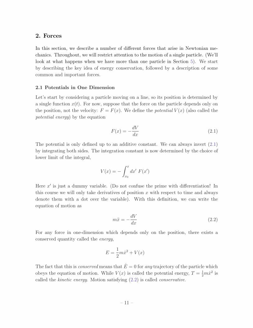
In this section, we describe a number of different forces that arise in Newtonian me-
chanics. Throughout, we will restrict attention to the motion of a single particle. (We’ll
look at what happens when we have more than one particle in Section 5). We start
by describing the key idea of energy conservation, followed by a description of some
common and important forces.
2.1 Potentials in One Dimension
Let’s start by considering a particle moving on a line, so its position is determined by
a single function x(t). For now, suppose that the force on the particle depends only on
the position, not the velocity: F = F (x). We define the potential V (x) (also called the
potential energy) by the equation
F (x) = −dVdx
(2.1)
The potential is only defined up to an additive constant. We can always invert (2.1)
by integrating both sides. The integration constant is now determined by the choice of
lower limit of the integral,
V (x) = −∫ x
x0
dx′ F (x′)
Here x′ is just a dummy variable. (Do not confuse the prime with differentiation! In
this course we will only take derivatives of position x with respect to time and always
denote them with a dot over the variable). With this definition, we can write the
equation of motion as
mx = −dVdx
(2.2)
For any force in one-dimension which depends only on the position, there exists a
conserved quantity called the energy,
E =1
2mx2 + V (x)
The fact that this is conserved means that E = 0 for any trajectory of the particle which
obeys the equation of motion. While V (x) is called the potential energy, T = 12mx2 is
called the kinetic energy. Motion satisfying (2.2) is called conservative.
– 11 –

It is not hard to prove that E is conserved. We need only differentiate to get
E = mxx+dV
dxx = x
(mx+
dV
dx
)= 0
where the last equality holds courtesy of the equation of motion (2.2).
In any dynamical system, conserved quantities of this kind are very precious. We
will spend some time in this course fishing them out of the equations and showing how
they help us simplify various problems.
An Example: A Uniform Gravitational Field
In a uniform gravitational field, a particle is subjected to a constant force, F = −mgwhere g ≈ 9.8 ms−2 is the acceleration due to gravity near the surface of the Earth.
The minus sign arises because the force is downwards while we have chosen to measure
position in an upwards direction which we call z. The potential energy is
V = mgz
Notice that we have chosen to have V = 0 at z = 0. There is nothing that forces us
to do this; we could easily add an extra constant to the potential to shift the zero to
some other height.
The equation of motion for uniform acceleration is
z = −g
Which can be trivially integrated to give the velocity at time t,
z = u− gt (2.3)
where u is the initial velocity at time t = 0. (Note that z is measured in the upwards
direction, so the particle is moving up if z > 0 and down if z < 0). Integrating once
more gives the position
z = z0 + ut− 1
2gt2 (2.4)
where z0 is the initial height at time t = 0. Many high schools teach that (2.3) and
(2.4) — the so-called “suvat” equations — are key equations of mechanics. They are
not. They are merely the integration of Newton’s second law for constant acceleration.
Do not learn them; learn how to derive them.
– 12 –

Another Simple Example: The Harmonic Oscillator
The harmonic oscillator is, by far, the most important dynamical system in all of
theoretical physics. The good news is that it’s very easy. (In fact, the reason that
it’s so important is precisely because it’s easy!). The potential energy of the harmonic
oscillator is defined to be
V (x) =1
2kx2
The harmonic oscillator is a good model for, among other things, a particle attached
to the end of a spring. The force resulting from the energy V is given by F = −kxwhich, in the context of the spring, is called Hooke’s law. The equation of motion is
mx = −kx
which has the general solution
x(t) = A cos(ωt) +B sin(ωt) with ω =
√k
m
Here A and B are two integration constants and ω is called the angular frequency. We
see that all trajectories are qualitatively the same: they just bounce backwards and
forwards around the origin. The coefficients A and B determine the amplitude of the
oscillations, together with the phase at which you start the cycle. The time taken to
complete a full cycle is called the period
T =2π
ω(2.5)
The period is independent of the amplitude. (Note that, annoyingly, the kinetic energy
is also often denoted by T as well. Do not confuse this with the period. It should
hopefully be clear from the context).
If we want to determine the integration constants A and B for a given trajectory, we
need some initial conditions. For example, if we’re given the position and velocity at
time t = 0, then it’s simple to check that A = x(0) and Bω = x(0).
2.1.1 Moving in a Potential
Let’s go back to the general case of a potential V (x) in one dimension. Although the
equation of motion is a second order differential equation, the existence of a conserved
energy magically allows us to turn this into a first order differential equation,
E =1
2mx2 + V (x) ⇒ dx
dt= ±
√2
m(E − V (x))
– 13 –

This gives us our first hint of the importance of conserved quantities in helping solve
a problem. Of course, to go from a second order equation to a first order equation, we
must have chosen an integration constant. In this case, that is the energy E itself. Given
a first order equation, we can always write down a formal solution for the dynamics
simply by integrating,
t− t0 = ±∫ x
x0
dx′√2m
(E − V (x′))(2.6)
As before, x′ is a dummy variable. If we can do the integral, we’ve solved the problem.
If we can’t do the integral, you sometimes hear that the problem has been “reduced to
quadrature”. This rather old-fashioned phrase really means “I can’t do the integral”.
But, it is often the case that having a solution in this form allows some of its properties
to become manifest. And, if nothing else, one can always just evaluate the integral
numerically (i.e. on your laptop) if need be.
Getting a Feel for the Solutions
Given the potential energy V (x), it is often very simple to figure out the qualitative
nature of any trajectory simply by looking at the form of V (x). This allows us to answer
some questions with very little work. For example, we may want to know whether the
particle is trapped within some region of space or can escape to infinity.
Let’s illustrate this with an example. Consider the cubic potential
V (x) = m(x3 − 3x) (2.7)
If we were to substitute this into the general form (2.6), we’d get a fearsome looking
integral which hasn’t been solved since Victorian times1.
Even without solving the integral, we can make progress. The potential is plotted
in Figure 2. Let’s start with the particle sitting stationary at some position x0. This
means that the energy is
E = V (x0)
and this must remain constant during the subsequent motion. What happens next
depends only on x0. We can identify the following possibilities
1Ok, I’m exaggerating. The resulting integral is known as an elliptic integral. Although it can’t
be expressed in terms of elementary functions, it has lots of nice properties and has been studied to
death. 100 years ago, this kind of thing was standard fare in mathematics. These days, we usually have
more interesting things to teach. Nonetheless, the study of these integrals later resulted in beautiful
connections to geometry through the theory of elliptic functions and elliptic curves.
– 14 –
V(x)
x
−1 +1
−2m
+2
2m
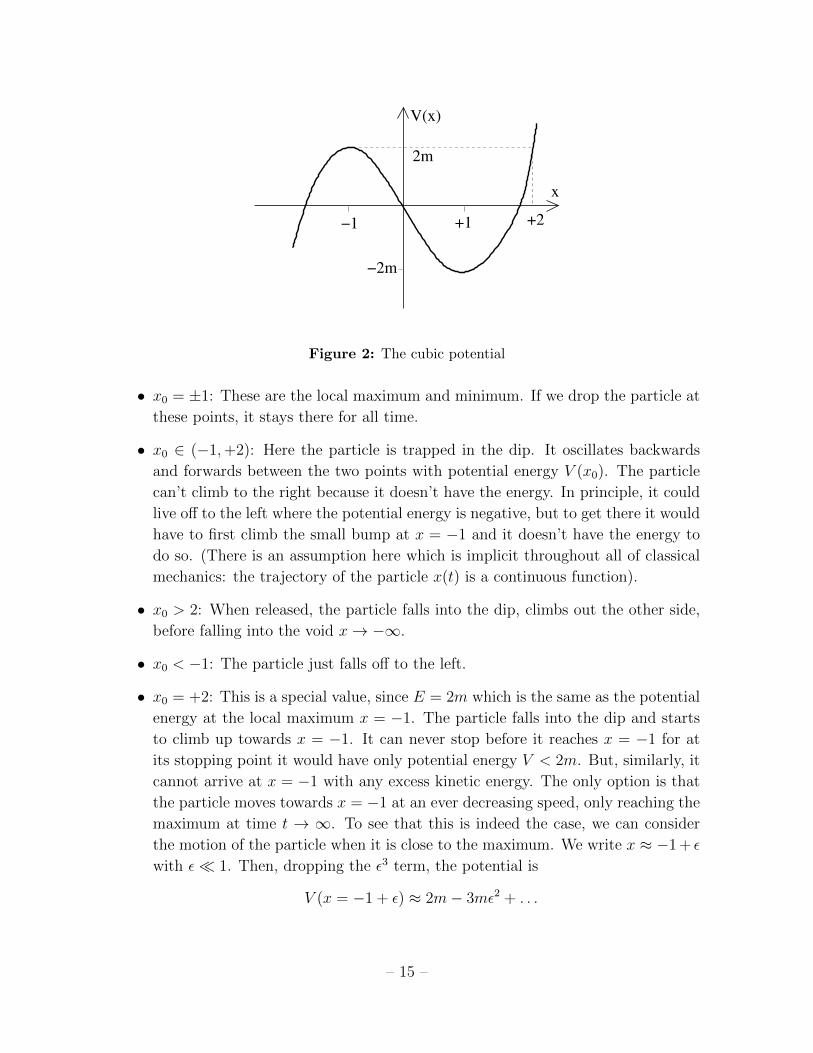
Figure 2: The cubic potential
• x0 = ±1: These are the local maximum and minimum. If we drop the particle at
these points, it stays there for all time.
• x0 ∈ (−1,+2): Here the particle is trapped in the dip. It oscillates backwards
and forwards between the two points with potential energy V (x0). The particle
can’t climb to the right because it doesn’t have the energy. In principle, it could
live off to the left where the potential energy is negative, but to get there it would
have to first climb the small bump at x = −1 and it doesn’t have the energy to
do so. (There is an assumption here which is implicit throughout all of classical
mechanics: the trajectory of the particle x(t) is a continuous function).
• x0 > 2: When released, the particle falls into the dip, climbs out the other side,
before falling into the void x→ −∞.
• x0 < −1: The particle just falls off to the left.
• x0 = +2: This is a special value, since E = 2m which is the same as the potential
energy at the local maximum x = −1. The particle falls into the dip and starts
to climb up towards x = −1. It can never stop before it reaches x = −1 for at
its stopping point it would have only potential energy V < 2m. But, similarly, it
cannot arrive at x = −1 with any excess kinetic energy. The only option is that
the particle moves towards x = −1 at an ever decreasing speed, only reaching the
maximum at time t → ∞. To see that this is indeed the case, we can consider
the motion of the particle when it is close to the maximum. We write x ≈ −1 + ε
with ε 1. Then, dropping the ε3 term, the potential is
V (x = −1 + ε) ≈ 2m− 3mε2 + . . .
– 15 –

and, using (2.6), the time taken to reach x = −1 + ε is
t− t0 = −∫ ε
ε0
dε′√6ε′
= − 1√6
log
(ε
ε0
)The logarithm on the right-hand side gives a divergence as ε → 0. This tells us
that it indeed takes infinite time to reach the top as promised.
One can easily play a similar game to that above if the starting speed is not zero. In
general, one finds that the particle is trapped in the dip x ∈ [−1,+1] if its energy lies
in the interval E ∈ [−2m, 2m].
2.1.2 Equilibrium: Why (Almost) Everything is a Harmonic Oscillator
A particle placed at an equilibrium point will stay there for all time. In our last example
with a cubic potential (2.7), we saw two equilibrium points: x = ±1. In general, if
we want x = 0 for all time, then clearly we must have x = 0, which, from the form of
Newton’s equation (2.2), tells us that we can identify the equilibrium points with the
critical points of the potential,
dV
dx= 0
What happens to a particle that is close to an equilibrium point, x0? In this case, we
can Taylor expand the potential energy about x = x0. Because, by definition, the first
derivative vanishes, we have
V (x) ≈ V (x0) +1
2V ′′(x0)(x− x0)2 + . . . (2.8)
To continue, we need to know about the sign of V ′′(x0):
• V ′′(x0) > 0: In this case, the equilibrium point is a minimum of the potential
and the potential energy is that of a harmonic oscillator. From our discussion of
Section 2.1.2, we know that the particle oscillates backwards and forwards around
x0 with frequency
ω =
√V ′′(x0)
m
Such equilibrium points are called stable. This analysis shows that if the ampli-
tude of the oscillations is small enough (so that we may ignore the (x−x0)3 terms
in the Taylor expansion) then all systems oscillating around a stable fixed point
look like a harmonic oscillator.
– 16 –

• V ′′(x0) < 0: In this case, the equilibrium point is a maximum of the potential.
The equation of motion again reads
mx = −V ′′(x0) (x− x0)
But with V ′′ < 0, we have x > 0 when x−x0 > 0. This means that if we displace
the system a little bit away from the equilibrium point, then the acceleration
pushes it further away. The general solution is
x− x0 = Aeαt +Be−αt with α =
√−V ′′(x0)
m
Any solution with the integration constant A 6= 0 will rapidly move away from
the fixed point. Since our whole analysis started from a Taylor expansion (2.8),
neglecting terms of order (x − x0)3 and higher, our approximation will quickly
break down. We say that such equilibrium points are unstable.
Notice that there are solutions around unstable fixed points with A = 0 and
B 6= 0 which move back towards the maximum at late times. These finely tuned
solutions arise in the kind of situation that we described for the cubic potential
where you drop the particle at a very special point (in the case of the cubic
potential, this point was x = 2) so that it just reaches the top of a hill in infinite
time. Clearly these solutions are not generic: they require very special initial
conditions.
• Finally, we could have V ′′(x0) = 0. In this case, there is nothing we can say about
the dynamics of the system without Taylor expanding the potential further.
Yet Another Example: The Pendulum
Consider a particle of mass m attached to the end of a light rod of
θ
m
length, l
T
mg
x
y
Figure 3:
length l. This counts as a one-dimensional system because we need
specify only a single coordinate to say what the system looks like at
a given time. The best coordinate to choose is θ, the angle that the
rod makes with the vertical. The equation of motion is
θ = −gl
sin θ (2.9)
The energy is
E =1
2ml2θ2 −mgl cos θ
(Note: Since θ is an angular variable rather than a linear variable, the kinetic energy is
a little different. Hopefully this is familiar from earlier courses on mechanics. However,
we will rederive this result in Section 4).
– 17 –

There are two qualitatively different motions of the pendulum. If E > mgl, then the
kinetic energy can never be zero. This means that the pendulum is making complete
circles. In contrast, if E < mgl, the pendulum completes only part of the circle before
it comes to a stop and swings back the other way. If the highest point of the swing is
θ0, then the energy is
E = −mgl cos θ0
We can determine the period T of the pendulum using (2.6). It’s actually best to
calculate the period by taking 4 times the time the pendulum takes to go from θ = 0
to θ = θ0. We have
T = 4
∫ T/4
0
dt = 4
∫ θ0
0
dθ√2E/ml2 + (2g/l) cos θ
= 4
√l
g
∫ θ0
0
dθ√2 cos θ − 2 cos θ0
(2.10)
We see that the period is proportional to√l/g multiplied by some dimensionless num-
ber given by (4 times) the integral. For what it’s worth, this integral turns out to be,
once again, an elliptic integral.
For small oscillations, we can write cos θ ≈ 1 − 12θ2 and the pendulum becomes a
harmonic oscillator with angular frequency ω =√g/l. If we replace the cos θ’s in (2.10)
by their Taylor expansion, we have
T = 4
√l
g
∫ θ0
0
dθ√θ2
0 − θ2= 4
√l
g
∫ 1
0
dx√1− x2
= 2π
√l
g
This agrees with our result (2.5) for the harmonic oscillator.
2.2 Potentials in Three Dimensions
Let’s now consider a particle moving in three dimensional R3. Here things are more
interesting. Firstly, it is possible to have energy conservation even if the force depends
on the velocity. We will see how this can happen in Section 2.4. Conversely, forces
which only depend on the position do not necessarily conserve energy: we need an extra
condition. For now, we restrict attention to forces of the form F = F(x). We have the
following result:
– 18 –
Claim: There exists a conserved energy if and only if the force can be written in
the form
F = −∇V (2.11)
for some potential function V (x). This means that the components of the force must
be of the form Fi = −∂V/∂xi. The conserved energy is then given by
E =1
2mx · x + V (x) (2.12)
Proof: The proof that E is conserved if F takes the form (2.11) is exactly the same as
in the one-dimensional case, together with liberal use of the chain rule. We have
dE
dt= mx · x +
∂V
∂xi∂xi
∂tusing summation convention
= x · (mx +∇V ) = 0
where the last equality follows from the equation of motion which is mx = −∇V .
To go the other way, we must prove that if there exists a conserved energy E taking
the form (2.12) then the force is necessarily given by (2.11). To do this, we need the
concept of work. If a force F acts on a particle and succeeds in moving it from x(t1)
to x(t2) along a trajectory C, then the work done by the force is defined to be
W =
∫CF · dx
This is a line integral (of the kind you’ve met in the Vector Calculus course). The
scalar product means that we take the component of the force along the direction of
the trajectory at each point. We can make this clearer by writing
W =
∫ t2
t1
F · dxdtdt
The integrand, which is the rate of doing work, is called the power, P = F · x. Using
Newton’s second law, we can replace F = mx to get
W = m
∫ t2
t1
x · x dt =1
2m
∫ t2
t1
d
dt(x · x) dt = T (t2)− T (t1)
where
T ≡ 1
2m x · x
is the kinetic energy. (You might think that K is a better name for kinetic energy. I’m
inclined to agree. Except in all advanced courses of theoretical physics, kinetic energy
is always denoted T which is why I’ve adopted the same notation here).
– 19 –

So the total work done is proportional to the change in kinetic energy. If we want to
have a conserved energy of the form (2.12), then the change in kinetic energy must be
equal to the change in potential energy. This means we must be able to write
W =
∫CF · dx = V (x(t1))− V (x(t2)) (2.13)
In particular, this result tells us that the work done must be independent of the tra-
jectory C; it can depend only on the end points x(t1) and x(t2). But a simple result
(which you will prove in your Vector Calculus course) says that (2.13) holds only for
forces of the form
F = −∇V
as required .
Forces in three dimensions which take the form F = −∇V are called conservative.
You will also see in the Vector Calculus course that forces in R3 are conservative if and
only if ∇× F = 0.
2.2.1 Central Forces
A particularly important class of potentials are those which depend only on the distance
to a fixed point, which we take to be the origin
V (x) = V (r)
where r = |x|. The resulting force also depends only on the distance to the origin and,
moreover, always points in the direction of the origin,
F(r) = −∇V = −dVdr
x (2.14)
Such forces are called central. In these lectures, we’ll also use the notation r = x to
denote the unit vector pointing radially from the origin to the position of the particle.
(In other courses, you may see this same vector denoted as er).
In the vector calculus course, you will spend some time computing quantities such
as ∇V in spherical polar coordinates. But, even without such practice, it is a simple
matter to show that the force (2.14) is indeed aligned with the direction to the origin.
If x = (x1, x2, x3) then the radial distance is r2 = x21 + x2
2 + x23, from which we can
– 20 –

compute ∂r/∂xi = xi/r for i = 1, 2, 3. Then, using the chain rule, we have
∇V =
(∂V
∂x1
,∂V
∂x2
,∂V
∂x3
)=
(dV
dr
∂r
∂x1
,dV
dr
∂r
∂x2
,dV
dr
∂r
∂x3
)=dV
dr
(x1
r,x2
r,x3
r
)=dV
drx
2.2.2 Angular Momentum
We will devote all of Section 4 to the study
x
L
x
Figure 4:
of motion in central forces. For now, we will
just mention what is important about central
forces: they have an extra conserved quantity.
This is a vector L called angular momentum,
L = mx× x
Notice that, in contrast to the momentum p = mx, the angular momentum L depends
on the choice of origin. It is a perpendicular to both the position and the momentum.
Let’s look at what happens to angular momentum in the presence of a general force
F. When we take the time derivative, we get two terms. But one of these contains
x× x = 0. We’re left with
dL
dt= mx× x = x× F
The quantity τ = x× F is called the torque. This gives us an equation for the change
of angular momentum that is very similar to Newton’s second law for the change of
momentum,
dL
dt= τ
Now we can see why central forces are special. When the force F lies in the same
direction as the position x of the particle, we have x × F = 0. This means that the
torque vanishes and angular momentum is conserved
dL
dt= 0
We’ll make good use of this result in Section 4 where we’ll see a number of important
examples of central forces.
– 21 –

2.3 Gravity
To the best of our knowledge, there are four fundamental forces in Nature. They are
• Gravity
• Electromagnetism
• Strong Nuclear Force
• Weak Nuclear Force
The two nuclear forces operate only on small scales, comparable, as the name suggests,
to the size of the nucleus (r0 ≈ 10−15m). We can’t really give an honest description of
these forces without invoking quantum mechanics and, for this reason, we won’t discuss
them in this course. (A very rough, and slightly dishonest, classical description of the
strong nuclear force can be given by the potential V (r) ∼ e−r/r0/r). In this section we
discuss the force of gravity; in the next, electromagnetism.
Gravity is a conservative force. Consider a particle of mass M fixed at the origin. A
particle of mass m moving in its presence experiences a potential energy
V (r) = −GMm
r(2.15)
Here G is Newton’s constant. It determines the strength of the gravitational force and
is given by
G ≈ 6.67× 10⁻¹¹ m3Kg−1s−2
The force on the particle is given by
F = −∇V = −GMm
r2r (2.16)
where r is the unit vector in the direction of the particle. This is Newton’s famous
inverse-square law for gravity. The force points towards the origin. We will devote
much of Section 4 to studying the motion of a particle under the inverse-square force.
2.3.1 The Gravitational Field
The quantity V in (2.15) is the potential energy of a particle of mass m in the presence
of mass M . It is common to define the gravitational field of the mass M to be
Φ(r) = −GMr
– 22 –
Φ is sometimes called the Newtonian gravitational field to distinguish it from a more
sophisticated object later introduced by Einstein. It is also sometimes called the grav-
itational potential. It is a property of the mass M alone. The potential energy of the
mass m is then given by V = mΦ.
The gravitational field due to many particles is simply the sum of the field due to
each individual particle. If we fix particles with masses Mi at positions ri, then the
total gravitational field is
Φ(r) = −G∑i
Mi
|r− ri|
The gravitational force that a moving particle of mass m experiences in this field is
F = −Gm∑i
Mi
|r− ri|3(r− ri)
The Gravitational Field of a Planet
The fact that contributions to the Newtonian gravitational potential add in a simple
linear fashion has an important consequence: the external gravitational field of a spher-
ically symmetric object of mass M – such as a star or planet – is the same as that of
a point mass M positioned at the origin.
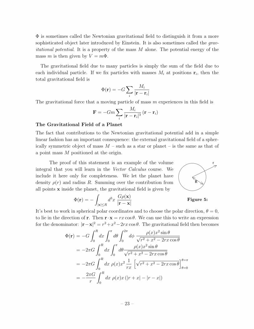
The proof of this statement is an example of the volume
R
r
Figure 5:
integral that you will learn in the Vector Calculus course. We
include it here only for completeness. We let the planet have
density ρ(r) and radius R. Summing over the contribution from
all points x inside the planet, the gravitational field is given by
Φ(r) = −∫|x|≤R
d3xGρ(x)
|r− x|It’s best to work in spherical polar coordinates and to choose the polar direction, θ = 0,
to lie in the direction of r. Then r ·x = rx cos θ. We can use this to write an expression
for the denominator: |r−x|2 = r2 +x2−2rx cos θ. The gravitational field then becomes
Φ(r) = −G∫ R
0
dx
∫ π
0
dθ
∫ 2π
0
dφρ(x)x2 sin θ√
r2 + x2 − 2rx cos θ
= −2πG
∫ R
0
dx
∫ π
0
dθρ(x)x2 sin θ√
r2 + x2 − 2rx cos θ
= −2πG
∫ R
0
dx ρ(x)x2 1
rx
[√r2 + x2 − 2rx cos θ
]θ=πθ=0
= −2πG
r
∫ R
0
dx ρ(x)x (|r + x| − |r − x|)
– 23 –

So far this calculation has been done for any point r, whether inside or outside the
planet. At this point, we restrict attention to points external to the planet. This
means that |r + x| = r + x and |r − x| = r − x and we have
Φ(r) = −4πG
r
∫ R
0
dx ρ(x)x2 = −GMr
This is the result that we wanted to prove: the gravitational field is the same as that
of a point mass M at the origin.
2.3.2 Escape Velocity
Suppose that you’re trapped on the the surface of a planet of radius R. (This should
be easy). Let’s firstly ask what gravitational potential energy you feel. Assuming you
can only rise a distance z R from the planet’s surface, we can Taylor expand the
potential energy,
V (R + z) = −GMm
R + z= −GMm
R
(1− z
R+z2
R2+ . . .
)If we’re only interested in small changes in z R, we need focus only on the second
term, giving
V (z) ≈ constant +GMm
R2z + . . .
This is the familiar potential energy that gives rise to constant acceleration. We usually
write g = GM/R2. For the Earth, g ≈ 9.8ms−2.
Now let’s be more ambitious. Suppose we want to escape our
Figure 6:
parochial, planet-bound existence. So we decide to jump. How fast
do we have to jump if we wish to truly be free? This, it turns out, is
the same kind of question that we discussed in Section 2.1.1 in the con-
text of particles moving in one dimension and can be determined very
easily using gravitational energy V = −GMm/r. If you jump directly
upwards (i.e. radially) with velocity v, your total energy as you leave
the surface is
E =1
2mv2 − GMm
R
For any energy E < 0, you will eventually come to a halt at position r = −GMm/E,
before falling back. If you want to escape the gravitational attraction of the planet for
– 24 –

ever, you will need energy E ≥ 0. At the minimum value of E = 0, the associated
velocity
vescape =
√2GM
R(2.17)
This is the escape velocity.
Black Holes and the Schwarzchild Radius
Let’s do something a little dodgy. We’ll take the formula above and apply it to light.
The reason that this is dodgy is because, as we will see in Section 7, the laws of
Newtonian physics need modifying for particles close to the speed of light where the
effects of special relativity are important. Nonetheless, let’s forget this for now and
plough ahead regardless.
Light travels at speed c ≈ 3× 10⁸ ms−1. Suppose that the escape velocity from the
surface of a star is greater than or equal to the speed of light. From (2.17), this would
happen if the radius of the star satisfies
R ≤ RS =2GM
c2
What do we see if this is the case? Well, nothing! The star is so dense that light can’t
escape from it. It’s what we call a black hole.
Although the derivation above is not trustworthy, by some fortunate coincidence
it turns out that the answer is correct. The distance Rs = 2GM/c2 is called the
Schwarzchild radius. If a star is so dense that it lies within its own Schwarzchild
radius, then it will form a black hole. (To demonstrate this properly, you really need
to work with the theory of general relativity).
For what it’s worth, the Schwarzchild radius of the Earth is around 1 cm. The
Schwarzchild radius of the Sun is about 3 km. You’ll be pleased to hear that, because
both objects are much larger than their Schwarzchild radii, neither is in danger of
forming a black hole any time soon.
2.3.3 Inertial vs Gravitational Mass
We have seen two formulae which involve mass, both due to Newton. These are the
second law (1.2) and the inverse-square law for gravity (2.16). Yet the meaning of
mass in these two equations is very different. The mass appearing in the second law
represents the reluctance of a particle to accelerate under any force. In contrast, the
– 25 –

mass appearing in the inverse-square law tells us the strength of a particular force,
namely gravity. Since these are very different concepts, we should really distinguish
between the two different masses. The second law involves the inertial mass, mI
mI x = F
while Newton’s law of gravity involves the gravitational mass, mG
F = −GMGmG
r2r
It is then an experimental fact that
mI = mG (2.18)
Much experimental effort has gone into determining the accuracy of (2.18), most no-
tably by the Hungarian physicist Eotvosh at the turn of the (previous) century. We
now know that the inertial and gravitational masses are equal to within about one part
in 1013. Currently, the best experiments to study this equivalence, as well as searches
for deviations from Newton’s laws at short distances, are being undertaken by a group
at the University of Washington in Seattle who go by the name Eot-Wash. A theoret-
ical understanding of the result (2.18) came only with the development of the general
theory of relativity.
2.4 Electromagnetism
Throughout the Universe, at each point in space, there exist two vectors, E and B.
These are known as the electric and magnetic fields. Their role – at least for the
purposes of this course – is to guide any particle that carries electric charge.
The force experienced by a particle with electric charge q is called the Lorentz force,
F = q(E(x) + x×B(x)
)(2.19)
Here we have used the notation E(x) and B(x) to stress that the electric and magnetic
fields are functions of space. Both their magnitude and direction can vary from point
to point.
The electric force is parallel to the electric field. By convention, particles with positive
charge q are accelerated in the direction of the electric field; those with negative electric
charge are accelerated in the opposite direction. Due to a quirk of history, the electron
is taken to have a negative charge given by
qelectron ≈ −1.6× 10⁻¹⁹ Coulombs
As far as fundamental physics is concerned, a much better choice is to simply say that
the electron has charge 1. All other charges can then be measured relative to this.
– 26 –

The magnetic force looks rather different. It is a velocity dependent force, with
magnitude proportional to the speed of the particle, but with direction perpendicular
to that of the particle. We shall see its effect in simple situations shortly.
In principle, both E and B can change in time. However, here we will consider only
situations where they are static. In this case, the electric field is always of the form
E = −∇φ
For some function φ(x) called the electric potential (or scalar potential or even just the
potential as if we didn’t already have enough things with that name).
For time independent fields, something special happens: energy is conserved.
Claim: The conserved energy is
E =1
2mx · x + qφ(x)
Proof:
E = mx · x + q∇φ · x = x · (F + q∇φ) = qx · (x×B) = 0
where the last equality occurs because x×B is necessarily perpendicular to x. Notice
that this gives an example of something we promised earlier: a velocity dependent force
which conserves energy. The key part of the derivation is that the velocity dependent
force is perpendicular to the trajectory of the particle. This ensures that the force does
no work. .
2.4.1 The Electric Field of a Point Charge
Charged objects do not only respond to electric fields; they also produce electric fields.
A particle of charge Q sitting at the origin will set up an electric field given by
E = −∇(
Q
4πε0r
)=
Q
4πε0
r
r2(2.20)
where r2 = x · x. The quantity ε0 has the grand name Permittivity of Free Space and
is a constant given by
ε0 ≈ 8.85× 10⁻¹² m−3Kg−1s2C2
This quantity should be thought of as characterising the strength of the electric inter-
action.
– 27 –

The force between two particles with charges Q and q is given by F = qE with E
given by (2.20). In other words,
F =qQ
4πε0
r
r2
This is known as the Coulomb force. It is a remarkable fact that, mathematically,
the force looks identical to the Newtonian gravitational force (2.16): both have the
characteristic inverse-square form. We will study motion in this potential in detail in
Section 4, with particular focus on the Coulomb force in 4.4.
Although the forces of Newton and Coulomb look the same, there is one important
difference. Gravity is always attractive because mass m > 0. In contrast, the electro-
static Coulomb force can be attractive or repulsive because charges q come with both
signs. Further differences between gravity and electromagnetism come when you ask
what happens when sources (mass or charge) move; but that’s a story that will be told
in different courses.
2.4.2 Circles in a Constant Magnetic Field
Motion in a constant electric field is simple: the particle undergoes constant acceleration
in the direction of E. But what about motion in a constant magnetic field B? The
equation of motion is
mx = q x×B
Let’s pick the magnetic field to lie in the z-direction and write
B = (0, 0, B)
We can now write the Lorentz force law (2.19) in components. It reads
mx = qBy (2.21)
my = −qBx (2.22)
mz = 0
The last equation is easily solved and the particle just travels at constant velocity in
the z direction. The first two equations are more interesting. There are a number of
ways to solve them, but a particularly elegant way is to construct the complex variable
ξ = x+ iy. Then adding (2.21) to i times (2.22) gives
mξ = −iqBξ
– 28 –

which can be integrated to give
ξ = αe−iωt + β
where α and β are integration constants and ω is given by
ω =qB
m
If we choose our initial conditions to be that the particle starts life at t = 0 at the
origin with velocity −v in the y-direction, then α and β are fixed to be
ξ =v
ω
(e−iωt − 1
)Translating this back into x and y coordinates, we have
x =v
ω(cosωt− 1) and y = − v
ωsinωt
The end result is that the particle undergoes circles in
x
y
B
Figure 7:
the plane with angular frequency ω, known as the cy-
clotron frequency The time to undergo a full circle is
fixed: T = 2π/ω. In contrast, the size of the circle is
v/ω and arises as an integration constant. Circles of ar-
bitrary sizes are allowed; the only price that you pay is
that you have to go faster.
A Comment on Solving Vector Differential Equa-
tions
The Lorentz force equation (2.19) gives a good example of a vector differential equation.
The straightforward way to view these is always in components: they are three, coupled,
second order differential equations for x, y and z. This is what we did above when
understanding the motion of a particle in a magnetic field.
However, one can also attack these kinds of questions without reverting to compo-
nents. Let’s see how this would work in the case of Larmor circles. We start with the
vector equation
mx = qx×B (2.23)
To begin, we take the dot product with B. Since the right-hand side vanishes, we’re
left with
x ·B = 0
– 29 –

This tells us that the particle travels with constant velocity in the direction of B. This
is simply a rewriting of our previous result z = 0. For simplicity, let’s just assume that
the particle doesn’t move in the B direction, remaining at the origin. This tells us that
the particle moves in a plane with equation
x ·B = 0 (2.24)
However, we’re not yet done. We started with (2.23) which was three equations. Taking
the dot product always reduces us to a single equation. So there must still be two further
equations lurking in (2.23) that we haven’t yet taken into account. To find them, the
systematic thing to do would be to take the cross product with B. However, in the
present case, it turns out that the simplest way forwards is to simply integrate (2.23)
once, to get
mx = qx×B + c
with c a constant of integration. We can now substitute this back into the right-hand
side of (2.23) to find
m2x = d + q2(x×B)×B
= d + q2 ((x ·B)B− (B ·B)x)
= −q2B2(x− d/q2B2
)where the integration constant now sits in d = qc × B which, by construction, is
perpendicular to B. In the last line, we’ve used the equation (2.24). (Note that if
we’d considered a situation in which the particle was moving with constant velocity
in the B direction, we’d have to work a little harder at this point). The resulting
vector equation looks like three harmonic oscillators, displaced by the vector d/q2B2,
oscillating with frequency ω = qB/m. However, because of the constraint (2.24), the
motion is necessarily only in the two directions perpendicular to B. The end result is
x =d
q2B2+α1 cosωt+α2 sinωt
with αi, i = 1, 2 integration constants satisfying αi ·B = 0. This is the same result we
found previously.
Admittedly, in this particular example, working with components was somewhat
easier than manipulating the vector equations directly. But this won’t always be the
case — for some problems you’ll make more progress by playing the kind of games that
we’ve described here.
– 30 –
2.4.3 An Aside: Maxwell’s Equations
In the Lorentz force law, the only hint that the electric and magnetic fields are related
is that they both affect a particle in a manner that is proportional to the electric charge.
The connection between them becomes much clearer when things depend on time. A
time dependent electric field gives rise to a magnetic field and vice versa. The dynamics
of the electric and magnetic fields are governed by Maxwell’s equations. In the absence
of electric charges, these equations are given by
∇ · E = 0 , ∇ ·B = 0
∇× E = −∂B
∂t, ∇×B =
1
c2
∂E
∂t
with c the speed of light. You will learn more about the properties of these equations
in the Electromagnetism and Electrodynamics courses.
For now, it’s worth making one small comment. When we showed that energy is
conserved, we needed both the electric and magnetic field to be time independent.
What happens when they change with time? In this case, energy is still conserved, but
we have to worry about the energy stored in the fields themselves.
2.5 Friction
Friction is a messy, dirty business. While energy is always conserved on a fundamental
level, it doesn’t appear to be conserved in most things that you do every day. If you
slide along the floor in your socks you don’t keep going for ever. At a microscopic level,
your kinetic energy is transferred to the atoms in the floor where it manifests itself as
heat. But if we only want to know how far our socks will slide, the details of all these
atomic processes are of little interest. Instead, we try to summarise everything in a
single, macroscopic force that we call friction.
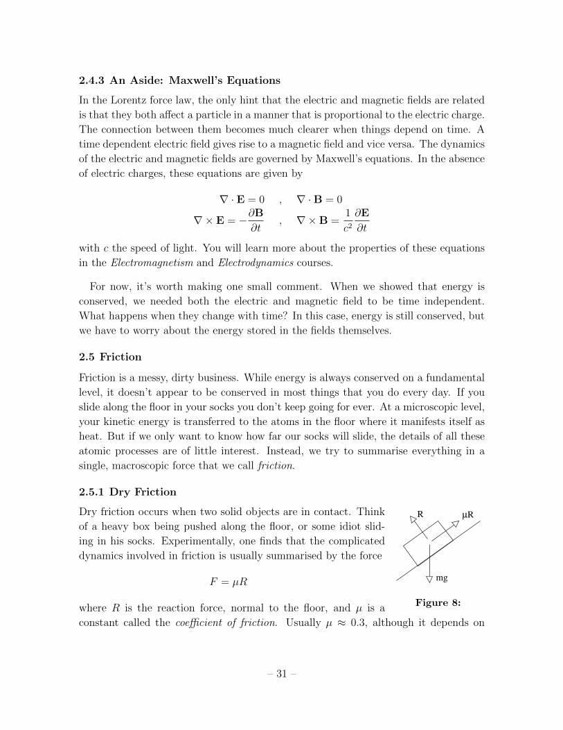
2.5.1 Dry Friction
Dry friction occurs when two solid objects are in contact. Think µRR
mg
Figure 8:
of a heavy box being pushed along the floor, or some idiot slid-
ing in his socks. Experimentally, one finds that the complicated
dynamics involved in friction is usually summarised by the force
F = µR
where R is the reaction force, normal to the floor, and µ is a
constant called the coefficient of friction. Usually µ ≈ 0.3, although it depends on
– 31 –
the kind of materials that are in contact. Moreover, the coefficient is usually, more or
less, independent of the velocity. We won’t have much to say about dry friction in this
course. In fact, we’ve already said it all.
2.5.2 Fluid Drag
Drag occurs when an object moves through a fluid — either liquid or gas. The resistive
force is opposite to the direction of the velocity and, typically, falls into one of two
categories
• Linear Drag:
F = −γv
where the coefficient of friction, γ, is a constant. This form of drag holds for
objects moving slowly through very viscous fluids. For a spherical object of
radius L, there is a formula due to Stokes which gives γ = 6πηL where η is the
viscosity of the fluid.
• Quadratic Drag:
F = −γ|v|v
Again, γ is called the coefficient of friction. For quadratic friction, γ is usually
proportional to the surface area of the object, i.e. γ ∼ L2. (This is in contrast to
the coefficient for linear friction where Stokes’ formula gives γ ∼ L). Quadratic
drag holds for fast moving objects in less viscous fluids. This includes objects
falling in air such as, for example, the various farmyard animals dropped by
Galileo from the leaning tower.
Quadratic drag arises because the object is banging into molecules in the fluid,
knocking them out the way. There is an intuitive way to see this. The force is
proportional to the change of momentum that occurs in each collision. That gives
one factor of v. But the force is also proportional to the number of collisions.
That gives the second factor of v, resulting in a force that scales as v2.
One can ask where the cross-over happens between linear and quadratic friction.
Naively, the linear drag must always dominate at low velocities simply because x x2
when x 1. More quantitatively, the type of drag is determined by a dimensionless
number called the Reynolds number,
R ≡ ρvL
η(2.25)
where ρ is the density of the fluid while η is the viscosity. For R 1, linear drag
dominates; for R 1, quadratic friction dominates.
– 32 –

What is Viscosity?
Above, we’ve mentioned the viscosity of the fluid, η, without really defining it. For
completeness, I will mention here how to measure viscosity.
Place a fluid between two plates, a distance d
v
d
Figure 9:
apart. Keeping the lower plate still, move the top plate
at a constant speed v. This sets up a velocity gradient
in the fluid. But, the fluid pushes back. To keep the
upper plate moving at constant speed, you will have to
push with a force per unit area which is proportional to
the velocity gradient,
F
A= η
v
d
The coefficient of proportionality, η, is defined to be the (dynamic) viscosity.
2.5.3 An Example: The Damped Harmonic Oscillator
We start with our favourite system: the harmonic oscillator, now with a damping term.
This was already discussed in your Differential Equations course and we include it here
only for completeness. The equation of motion is
mx = −kx− γx
Divide through by m to get
x = −ω20x− 2αx
where ω20 = k/m is the frequency of the undamped harmonic oscillator and α = γ/2m.
We can look for solutions of the form
x = eiβt
Remember that x is real, so we’re using a trick here. We rely on the fact that the
equation of motion is linear so that if we can find a solution of this form, we can take
the real and imaginary parts and this will also be a solution. Substituting this ansatz
into the equation of motion, we find a quadratic equation for β. Solving this, gives the
general solution
x = Aeiω+t +Beiω−t
with ω± = iα±√ω2
0 − α2. We identify three different regimes,
– 33 –

• Underdamped: ω20 > α2. Here the solution takes the form,
x = e−αt(AeiΩt +Be−iΩt
)where Ω =
√ω2 − α2. Here the system oscillates with a frequency Ω < ω0, while
the amplitude of the oscillations decays exponentially.
• Overdamped: ω20 < α2. The roots ω± are now purely imaginary and the general
solution takes the form,
x = e−αt(AeΩt +Be−Ωt
)Now there are no oscillations. Both terms decay exponentially. If you like, the
amplitude decays away before the system is able to undergo even a single oscil-
lation.
• Critical Damping: ω20 = α2. Now the two roots ω± coincide. With a double root
of this form, the most general solution takes the form,
x = (A+Bt)e−αt
Again, there are no oscillations, but the system does achieve some mild linear
growth for times t < 1/α, after which it decays away.
2.5.4 Terminal Velocity with Quadratic Friction
You can drop a mouse down a thousand-yard mine shaft; and, on arriving
at the bottom, it gets a slight shock and walks away, provided that the ground
is fairly soft. A rat is killed, a man is broken, a horse splashes.
J.B.S. Haldane, On Being the Right Size
Let’s look at a particle of mass m moving in a constant gravitational field, subject to
quadratic friction. We’ll measure the height z to be in the upwards direction, meaning
that if v = dz/dt > 0, the particle is going up. We’ll look at the cases where the
particle goes up and goes down separately.
Coming Down
Suppose that we drop the particle from some height. The equation of motion is given
by
mdv
dt= −mg + γv2
– 34 –

It’s worth commenting on the minus signs on the right-hand side. Gravity acts down-
wards, so comes with a minus sign. Since the particle is falling down, friction is acting
upwards so comes with a plus sign. Dividing through by m, we have
dv
dt= −g +
γv2
m(2.26)
Integrating this equation once gives
t = −∫ v
0
dv′
g − γv′ 2/m
which can be easily solved by the substitution v =√mg/γ tanhx to get
t = −√m
γgtanh−1
(√γ
mgv
)Inverting this gives us the speed as a function of time
v = −√mg
γtanh
(√γg
mt
)We now see the effect of friction. As time increases, the velocity does not increase
without bound. Instead, the particle reaches a maximum speed,
v → −√mg
γas t→∞ (2.27)
This is the terminal velocity. The sign is negative because the particle is falling down-
wards. Notice that if all we wanted was the terminal velocity, then we don’t need to go
through the whole calculation above. We can simply look for solutions of (2.26) with
constant speed, so dv/dt = 0. This obviously gives us (2.27) as a solution. The advan-
tage of going through the full calculation is that we learn how the velocity approaches
its terminal value.
We can now see the origin of the quote we started with. The point is that if we
compare objects of equal density, the masses scale as the volume, meaning m ∼ L3
where L is the linear size of the object. In contrast, the coefficient of friction usually
scales as surface area, γ ∼ L2. This means that the terminal velocity depends on size.
For objects of equal density, we expect the terminal velocity to scale as v ∼√L. I have
no idea if this is genuinely a big enough effect to make horses splash. (Haldane was a
biologist, so he should know what it takes to make an animal splash. But in his essay
he assumed linear drag rather than quadratic, so maybe not).
– 35 –

Going Up
Now let’s think about throwing a particle upwards. Since both gravity and friction are
now acting downwards, we get a flip of a minus sign in the equation of motion. It is
now
dv
dt= −g − γv2
m(2.28)
Suppose that we throw the object up with initial speed u and we want to figure out
the maximum height, h, that it reaches. We could follow our earlier calculation and
integrate (2.28) to determine v = v(t). But since we aren’t asking about time, it’s
much better to instead consider velocity as a function of distance: v = v(z). We write
dv
dt=dv
dz
dz
dt= v
dv
dz= −g − γv2
m
which can be rewritten as
1
2
d(v2)
dz= −g − γv2
m
Now we can integrate this equation to get velocity as a function of distance. Writing
y = v2, we have∫ 0
u2
dy
g + γy/m= −2
∫ h
0
dz ⇒ m
γ
[log(g +
γy
m
)]y=0
y=u2= −2h
which we can rearrange to get the final answer,
h =m
2γlog
(1 +
γu2
mg
)It’s worth looking at what happens when the effect of friction is small. Naively, it
looks like we’re in trouble here because as γ → 0, the term in front gets very large.
But surely the height shouldn’t go to infinity just because the friction is small. The
resolution to this is that the log is also getting small in this limit. Expanding the log,
we have
h =u2
2g
(1− γu2
2mg+ . . .
)Here the leading term is indeed the answer we would get in the absence of friction; the
subleading terms tell us how much the friction, γ, lowers the attained height.
– 36 –

Linear Drag and Ohm’s Law
Consider an electron moving in a conductor. As we’ve seen, a constant electric field
causes the electron to accelerate. A fairly good model for the physics of a conduc-
tor, known as the Drude model, treats the electron as a classical particle with linear
damping. The resulting equation of motion is
mx = −eE − γv
As in the previous example, we can figure out the terminal velocity by setting x = 0,
to get
v = −eEγ
In a conductor, the velocity of the electron v gives the current density, j,
j = −env
where n is the density of electrons. This then gives us a relationship between the
current density and the electric field
j = σE
The quantity σ = e2n/γ is called the conductivity. This equation is Ohm’s law. How-
ever, it’s probably not yet in the form you know and love. If the wire has length L and
cross-sectional area A, then the current I is defined as I = jA. Meanwhile, the voltage
dropped across the wire is V = EL. With this in hand, we can rewrite Ohm’s law as
V = IR
where the resistance is given by R = L/σA.
A 3d Example: A Projectile with Linear Drag
All our examples so far have been effectively one-dimensional. Here we give a three
dimensional example which provides another illustration of how to treat vector differ-
ential equations and, specifically, how to work with vector constants on integration.
We will consider a projectile, moving under gravity, experiencing linear drag. (Think
of a projectile moving very slowly in a viscous liquid). At time t = 0, we throw the
object with velocity u. What is its subsequent motion?
– 37 –

The equation of motion is
mdv
dt= mg − γv (2.29)
We can solve this by introducing the integrating factor eγt/m to write the equation as
d
dt
(eγt/mv
)= eγt/mg
We now integrate, but have to introduce a vector integration constant – let’s call it c
– for our troubles. We have
v =m
γg + ce−γt/m
We specified above that at time t = 0, the velocity is v = u, so we can use this
information to determine the integration constant c. We get
v =m
γg +
(u− m
γg
)e−γt/m
Now we integrate v = dx/dt a second time to determine x as a function of time. We
get another integration constant, b,
x =m
γgt− m
γ
(u− m
γg
)e−γt/m + b
To determine this second integration constant, we need some further information about
the initial conditions. Lets say that x = 0 at t = 0. Then we have
x =m
γgt+
m
γ
(u− m
γg
)(1− e−γt/m
)We can now look at this in components to get a better idea of what’s going on.
We’ll write x = (x, y, z) and we’ll send the projectile off with initial velocity u =
(u cos θ, 0, u sin θ). With gravity acting downwards, so g = (0, 0,−g), our vector equa-
tion becomes three equations. One is trivial: y = 0. The other two are
x =m
γu cos θ
(1− e−γt/m
)z = −mgt
γ+m
γ
(u sin θ +
mg
γ
)(1− e−γt/m
)Notice that the time scale m/γ is important. For t m/γ, the horizontal position is
essentially constant. By this time, the particle is dropping more or less vertically.
– 38 –

Finally, we can revisit the question that we asked in the last example: what happens
when friction is small? Again, there are a couple of terms that look as if they are
going to become singular in this limit. But that sounds very unphysical. To resolve
this, we should ask what γ is small relative to. In the present case, the answer lies
in the exponential terms. To say that γ is small, really means γ m/t or, in other
words, it means that we are looking at short times, t m/γ. Then we can expand the
exponential. Reverting to the vector form of the equation, we find
x =m
γgt+
m
γ
(u− m
γg
)(1− 1 +
γt
m− 1
2
(γt
m
)2
+ . . .
)
= ut+1
2gt2 +O
(γt
m
)So we see that, on small time scales, we indeed recover the usual story of a projectile
without friction. The friction only becomes relevant when t ∼ m/γ.
– 39 –
3. Interlude: Dimensional Analysis
The essence of dimensional analysis is very simple: if you are asked how hot it is outside,
the answer is never “2 o’clock”. You’ve got to make sure that the units agree. Quantities
which come with units are said to have dimensions. In contrast, pure numbers such as
2 or π are said to be dimensionless.
In all the examples that we met in the previous section, the units are hiding within
the variables. Nonetheless, it’s worth our effort to dig them out. In most situations,
it is useful to identify three fundamental dimensions: length L, mass M and time T .
The dimensions of all other quantities should be expressible in terms of these. We will
denote the dimension of a quantity Y as [Y ]. Some basic examples include,
[Area] = L2
[Speed] = LT−1
[Acceleration] = LT−2
[Force] = MLT−2
[Energy] = ML2T−2
The first three should be obvious. You can quickly derive the last two by thinking of
your favourite equation and insisting that the dimensions on both sides are consistent.
For example, F = ma immediately gives the dimensions [F ], while E = 12mv2 will give
you the dimensions [E]. This same technique can be used to determine the dimensions of
any constants that appear in equations. For example, Newton’s gravitational constant
appears in the formula F = −GMm/r2. Matching dimensions on both sides tells us
that
[G] = M−1L3T−2
You shouldn’t be too dogmatic in insisting that there are exactly three dimensions of
length, mass and time. In some problems, it will be useful to introduce further dimen-
sions such as temperature or electric charge. For yet other problems, it could be useful
to distinguish between distances in the x-direction and distances in the z-direction. For
example, if you’re a sailor, you would be foolish to think of vertical distances in the
same way as horizontal distances. Your life is very different if you mistakenly travel 10
fathoms (i.e. vertically) instead of 10 nautical miles (i.e. horizontally) and it’s useful
to introduce different units to reflect this.
– 40 –

Conversely, when dealing with matters in fundamental physics, we often reduce the
number of dimensional quantities. As we will see in Section 7, in situations where special
relativity is important, time and space sit on the same footing and can be measured in
the same unit, with the speed of light providing a conversion factor between the two.
(We’ll have more to say on this in Section 7.3.3). Similarly, in statistical mechanics,
Boltzmann’s constant provides a conversion factor between temperature and energy.
Scaling: Bridgman’s Theorem
Any equation that we derive must be dimensionally consistent. This simple observation
can be a surprisingly powerful tool. Firstly, it provides a way to quickly check whether
an answer has a hope of being correct. (And can be used to spot where a mistake
appeared in a calculation). Moreover, there are certain problems that can be answered
using dimensional analysis alone, allowing you to avoid calculations all together. Let’s
look at this in more detail.
We start by noting that dimensionful quantities such as length can only appear in
equations as powers, Lα for some α. We can never have more complicated functions.
One simple way to see this is to Taylor expand. For example, the exponential function
has the Taylor expansion
ex = 1 + x+x2
2+ . . .
The right-hand side contains all powers of x and only makes sense if x is a dimensionless
quantity: we can never have eL appearing in an exponent otherwise we’d be adding a
length to an area to a volume and so on. A similar statement holds for sinx and log x,
for your favourite and least favourite functions. In all cases, the argument must be
dimensionless unless the function is simply of the form xα. (If your favourite function
doesn’t have a Taylor expansion around x = 0, simply expand around a different point
to reach the same conclusion).
Suppose that we want to compute some quantity Y . This must have dimension
[Y ] = MαLβT γ
for some α, β and γ. (There is, in general, no need for these to be integers although
they are typically rational). We usually want to determine Y in terms of various
other quantities in the game – call them Xi, with i = 1, . . . n. These too will have
certain dimensions. We’ll focus on just three of them, X1, X2 and X3. We’ll assume
that these three quantities are “dimensionally independent”, meaning that by taking
– 41 –
suitable combinations of X1, X2 and X3, we can build quantities with dimension of
length, mass and time. Then we must be able to express Y as
Y = C Xa11 X
a22 X
a33
for some a1, a2 and a3 such that
[Xa11 ] [Xa2
2 ] [Xa33 ] = MαLβT γ
which is simply the requirement that the dimensions agree on both sides. All the
difficulty of the problem has been swept into determining C which, by necessity, is
dimensionless. In principle, C can depend on all the Xi. However, since C is dimen-
sionless, it can only depend on combinations of Xi which are also dimensionless. And
this will often greatly restrict the form that the answer can take.
An Example: The Pendulum
The above discussion is a little abstract. Let’s throw some light on it with a simple
example. We will consider a pendulum. We already discussed the pendulum earlier in
(2.9). It has equation of motion
θ = −gl
sin θ
We’d like to know the period, T . This plays the role of the quantity we called Y above:
clearly, it has dimension of time. (Although we’ve picked a slightly annoying choice of
notation because we have the equation [T ] = T . Hopefully it won’t cause too much
confusion).
What are the variables Xi that the period can depend upon? There are four of them:
the strength of gravity g, the mass of the pendulum m, the length of the pendulum
l and the initial starting angle θ0. The dimension of m and l are obviously mass and
length respectively; the dimension of acceleration is [g] = LT−2 while the initial angle
is necessarily dimensionless [θ0] = 0. (This follows from its periodicity, θ = θ + 2π,
because 2π is dimensionless; alternatively it follows from the fact that it sits as the
argument of a sin function). The only dimensionless combination that we can form is
θ0 itself. We can therefore write
T = C(θ0) ga1ma2la3
where, on dimensional grounds, we must have
[T ] = T = [ga1 ] [ma2 ] [la3 ] = Ma2La1+a3T−2a1
– 42 –
The unique solution is a2 = 0 and a1 = −a3 = −12. We learn immediately that
T = C(θ0)
√l
g(3.1)
This agrees with the result (2.10) that we got the hard way by solving the equation
of motion. Of course we haven’t solved the problem completely; by using dimensional
analysis there’s no way to figure out the function C(θ0) which is given by the elliptic
integral in (2.10).
Nonetheless, there’s important information contained in the form (3.1). For example,
it tells us that the mass of the pendulum doesn’t affect the period. Moreover, suppose
you are given two pendulums, with lengths l1 and l2. You release them from the same
starting angle and want to know how much faster the first pendulum swings compared
to the second. For these kinds of comparative questions, the unknown function C(θ0)
drops out, and we can just immediately write down the result:
T1
T2
=
√l1l2
Whenever we are interested only in how things scale with some quantity, it is conven-
tional to use the symbol ∼. (We could also use the proportional symbol ∝ but it looks
a little too much like the Greek letter α). So equation (3.1) would be written as
T ∼
√l
g
In fact we already used this notation a number of times in the last Section.
The Importance of Dimensionless Quantities
The power of dimensional analysis really depends on how many dimensionless quantities
we can construct from the variables at hand. If we can construct r dimensionless
variables, then the unknown dimensionless quantity C is a function of r variables. In
problems where r = 0 and there are no dimensionless combinations of variables, then
C is just a number.
It is a simple matter to count the number of dimensionless parameters in a given
problem. If we have n independent variables Xi in a problem that requires k indepen-
dent dimensions then we will be able to form r = n − k dimensionless combinations.
(In our discussion above, we had k = 3 corresponding to mass, length and time). This
– 43 –

intuitive result goes by the grand name of the Buckingham Π theorem. It can be proved
formally by setting up a system of linear equations and invoking the rank-nullity theo-
rem of linear algebra. Finally, the dimensionless combinations that you can make in a
given problem are not unique: if x and y are both dimensionless, then so are xy and x2y
and x+ y and, indeed, any function that you want to make out of these two variables.
There are other reasons to be interested in dimensionless quantities. The first is
practical: identifying dimensionless quantities at an early stage in a calculation will
save you ink! In a calculation that contains lots of variables, you’ll often find the
same dimensionless combinations of variables appearing at every stage. In particular
– as we’ve already seen – it is only dimensionless combinations that can appear as the
arguments of functions. Often, identifying these combinations at an early stage — and
perhaps even giving them a name of their own — will speed up the computation and
help in avoiding errors.
For example, if we look back to the problem of the 3d projectile with linear friction,
with equation of motion (2.29), we see that the dimensionless combination γt/m ap-
pears over and over in all steps of the calculation. In this case, it wasn’t too annoying to
keep writing γt/m. But if you find yourself doing a calculation where the combination
e2me/2πε0~2r appears three times on every line, then it’s a good idea to come up with
a new name for this object.
The second reason to be interested in dimensionless quantities is because the answer
to a calculation often simplifies in certain regimes. Perhaps this is the regime of long
times, or short distances, or high speeds, or some such thing. But only dimensionless
numbers can be big. For a dimensionless quantity x, we can write x 1. But it makes
no sense to write Y 1 if Y is not dimensionless: a dimensionful quantity must always
be big or small relative to something else.
We already discussed this issue in the case of the projectile (2.29), where we saw
that long times necessarily meant tγ/m 1. This is also the reason that we needed
to introduce a dimensionless quantity, the Reynolds number (2.25), to decide which
systems suffer linear friction vs quadratic friction.
Another Example: The Atomic Bomb
In the 1950s, the fluid dynamicist G.I. Taylor applied dimensional analysis to pho-
tographs of an atomic explosion. As you can see in the example below, these pho-
tographs happily came with both a time scale and distance scale, allowing you to trace
the radius of the shock front R(t) as a function of time after the explosion. To the
– 44 –

annoyance of the US government, Taylor was able to use these time and distance scales
to get a good estimate of the energy released in the explosion. At the time this was
classified information.
For most explosions, the dynamics of the shock
Figure 10:
front depends on the pressure of the outside air. Tay-
lor’s insight was to realise that in an explosion as pow-
erful as an atomic bomb, the air pressure is completely
negligible. However, the density of air, ρ, is important.
Taylor identified the following relevant variables
Air density [ρ] = ML−3
Shock Front Radius [R] = L
Time from Explosion [t] = T
There are no dimensionless quantities that we can build
from these. Since the energy released in the explosion has dimension [E] = ML2T−2,
on dimensional grounds we must have
E = CρR5
t2
where C is an unknown constant. Of course, without knowing C this would seem to
be useless. In Taylor’s case, a few further supplementary calculations allowed him to
estimate C.
In general, there’s a good rule of thumb if you want to figure out unknown constants
such as C: once you’ve figured out how many factors of 2π they contain, what’s left is
almost always a number that’s close to one. With a little bit of experience, it’s usually
possible to guess the factors of 2π as well.
A Last Example: Rowing
Another, classic demonstration of the power of dimensional analysis is in understanding
how the speed of a rowing boat depends on the number of rowers2.
The boat experiences quadratic friction, proportional to the submerged cross-sectional
area A of the boat.
Fdrag ∼ v2A
2This analysis was first by T. McMahon in the paper “Rowing: A similarity analysis”, Science
173:349 (1971)
– 45 –

(On dimensional grounds, we actually have F ∼ ρv2A, where ρ is the density of water,
but this will not be important for our story). The power needed to overcome the drag
is therefore
P = Fdragv ∼ v3A
By Archimedes’ law, the displaced volume increases linearly with the number of rowers,
N . This means that the submerged volume V ∼ N so the submerged area scales as
A ∼ N2/3. (We are assuming here that the mass of the boat is negligible compared to
the mass of the rowers). Meanwhile, if we further assume that the power supplied by
each rower is the same, we have P ∼ N . Putting all this together, we have P ∼ N ∼v3N2/3. Rearranging, we learn that the velocity increases with the number of rowers as
v ∼ N1/9
This simple result actually agrees pretty well with Olympic rowing times.
Dimensional Constants of Nature
The laws of physics provide us with three fundamental constants of Nature. We have
already met G ≈ 6.7×10⁻¹¹ m3Kg−1s−2 which appears in both Newton’s law of gravity
as well as the more refined theory of gravity due to Einstein known as general relativity.
The other two fundamental constants are the speed of light, c ≈ 3× 10⁸ ms−1, which
characterises the relationship between space and time in special relativity, and Planck’s
constant ~ ≈ 10−34 Js which determines when quantum effects become important.
These constants have dimensions
[G] = M−1L3T−2 , [c] = LT−1 , [~] = ML2T−1
From these three constants, we can construct a characteristic length scale, known as
the Planck length lp
lp =
√G~c3≈ 10−35m
This is the distance at which gravity, quantum mechanics and the structure of space-
time all become important. All indications are that this is the shortest distance scale
possible; at distances shorter than lp, space itself is likely to have no meaning. Simi-
larly, we can define the Planck time, tp = lp/c, the Planck mass mp =√
~c/G and the
Planck energy,
Ep =~clp≈ 1019 GeV
– 46 –

where 1 GeV ≈ 10−10 J is a measure of energy used in particle physics. If we want
to explore aspects of quantum gravity in experiments on Earth, we will need to build
particle colliders capable of reaching Planck energies. This is a long way off: the LHC
operates at energies around 104 GeV .
– 47 –

4. Central Forces
In this section we will study the three-dimensional motion of a particle in a central
force potential. Such a system obeys the equation of motion
mx = −∇V (r) (4.1)
where the potential depends only on r = |x|. Since both gravitational and electrostatic
forces are of this form, solutions to this equation contain some of the most important
results in classical physics.
Our first line of attack in solving (4.1) is to use angular momentum. Recall that this
is defined as
L = mx× x
We already saw in Section 2.2.2 that angular momentum is conserved in a central
potential. The proof is straightforward:
dL
dt= mx× x = −x×∇V = 0
where the final equality follows because ∇V is parallel to x.
The conservation of angular momentum has an important consequence: all motion
takes place in a plane. This follows because L is a fixed, unchanging vector which, by
construction, obeys
L · x = 0
So the position of the particle always lies in a plane perpendicular to L. By the same
argument, L · x = 0 so the velocity of the particle also lies in the same plane. In this
way the three-dimensional dynamics is reduced to dynamics on a plane.
4.1 Polar Coordinates in the Plane
We’ve learned that the motion lies in a plane. It will turn out to be much easier if we
work with polar coordinates on the plane rather than Cartesian coordinates. For this
reason, we take a brief detour to explain some relevant aspects of polar coordinates.
To start, we rotate our coordinate system so that the angular momentum points in
the z-direction and all motion takes place in the (x, y) plane. We then define the usual
polar coordinates
x = r cos θ , y = r sin θ
– 48 –

Our goal is to express both the velocity and acceleration ^r^
θ
θ x
y
Figure 11:
in polar coordinates. We introduce two unit vectors, r
and θ in the direction of increasing r and θ respectively
as shown in the diagram. Written in Cartesian form,
these vectors are
r =
(cos θ
sin θ
), θ =
(− sin θ
cos θ
)
These vectors form an orthornormal basis at every point
on the plane. But the basis itself depends on which angle θ we sit at. Moving in the
radial direction doesn’t change the basis, but moving in the angular direction we have
dr
dθ=
(− sin θ
cos θ
)= θ ,
dθ
dθ=
(− cos θ
− sin θ
)= −r
This means that if the particle moves in a way such that θ changes with time, then the
basis vectors themselves will also change with time. Let’s see what this means for the
velocity expressed in these polar coordinates. The position of a particle is written as
the simple, if somewhat ugly, equation
x = rr
From this we can compute the velocity, remembering that both r and the basis vector
r can change with time. We get
x = rr + rdr
dθθ
= rr + rθθ (4.2)
The second term in the above expression arises because the basis vectors change with
time and is proportional to the angular velocity, θ. (Strictly speaking, this is the angular
speed. In the next section, we will introduce a vector quantity which is the angular
velocity).
Differentiating once more gives us the expression for acceleration in polar coordinates,
x = rr + rdr
dθθ + rθθ + rθθ + rθ
dθ
dθθ
= (r − rθ2)r + (rθ + 2rθ)θ (4.3)
The two expressions (4.2) and (4.3) will be important in what follows.
– 49 –

An Example: Circular Motion
Let’s look at an example that we’re already all familiar with. A particle moving in a
circle has r = 0. If the particle travels with constant angular velocity θ = ω then the
velocity in the plane is
x = rωθ
so the speed in the plane in v = |x| = rω. Similarly, the acceleration in the plane is
x = −rω2r
The magnitude of the acceleration is a = |x| = rω2 = v2/r. From Newton’s second
law, if we want a particle to travel in a circle, we need to supply a force F = mv2/r
towards the origin. This is known as a centripetal force.
4.2 Back to Central Forces
We’ve already seen that the three-dimensional motion in a central force potential ac-
tually takes place in a plane. Let’s write the equation of motion (4.1) using the plane
polar coordinates that we’ve just introduced. Since V = V (r), the force itself can be
written using
∇V =dV
drr
and, from (4.3) the equation of motion becomes
m(r − rθ2)r +m(rθ + 2rθ)θ = −dVdr
r (4.4)
The θ component of this is particularly simple. It is
rθ + 2rθ = 0 ⇒ 1
r
d
dt
(r2θ)
= 0
It looks as if we’ve found a new conserved quantity since we’ve learnt that
l = r2θ (4.5)
does not change with time. However, we shouldn’t get too excited. This is something
that we already know. To see this, let’s look again at the angular momentum L. We
already used the fact that the direction of L is conserved when restricting motion to
the plane. But what about the magnitude of L? Using (4.2), we write
L = mx× x = mrr×(rr + rθθ
)= mr2θ
(r× θ
)
– 50 –

Since r and θ are orthogonal, unit vectors, r× θ is also a unit vector. The magnitude
of the angular momentum vector is therefore
|L| = ml
and l, given in (4.5), is identified as the angular momentum per unit mass, although
we will often be lazy and refer to l simply as the angular momentum.
Let’s now look at the r component of the equation of motion (4.4). It is
m(r − rθ2) = −dVdr
Using the fact that l = r2θ is conserved, we can write this as
mr = −dVdr
+ml2
r3(4.6)
It’s worth pausing to reflect on what’s happened here. We started in (4.1) with a com-
plicated, three dimensional problem. We used the direction of the angular momentum
to reduce it to a two dimensional problem, and the magnitude of the angular momen-
tum to reduce it to a one dimensional problem. This was all possible because angular
momentum is conserved.
This should give you some idea of how important conserved quantities are when it
comes to solving anything. Roughly speaking, this is also why it’s not usually possible
to solve the N -body problem with N ≥ 3. In Section 5.1.5, we’ll see that for the N = 2
mutually interacting particles, we can use the symmetry of translational invariance to
solve the problem. But for N ≥ 3, we don’t have any more conserved quantities to
come to our rescue.
Returning to our main storyline, we can write (4.6) in the suggestive form
mr = −dVeff
dr(4.7)
where Veff(r) is called the effective potential and is given by
Veff(r) = V (r) +ml2
2r2(4.8)
The extra term, ml2/2r2 is called the angular momentum barrier (also known as the
centrifugal barrier). It stops the particle getting too close to the origin, since there is
must pay a heavy price in“effective energy”.
– 51 –

Veff
r
Emin
r*
Figure 12: The effective potential arising from the inverse square force law.
4.2.1 The Effective Potential: Getting a Feel for Orbits
Let’s just check that the effective potential can indeed be thought of as part of the
energy of the full system. Using (4.2), we can write the energy of the full three dimen-
sional problem as
E =1
2mx · x + V (r)
=1
2mr2 +
1
2mr2θ2 + V (r)
=1
2mr2 +
ml2
2r2+ V (r)
=1
2mr2 + Veff(r)
This tells us that the energy E of the three dimensional system does indeed coincide
with the energy of the effective one dimensional system that we’ve reduced to. The
effective potential energy is the real potential energy, together with a contribution from
the angular kinetic energy.
We already saw in Section 2.1.1 how we can understand qualitative aspects of one
dimensional motion simply by plotting the potential energy. Let’s play the same game
here. We start with the most useful example of a central potential: V (r) = −k/r,corresponding to an attractive inverse square law for k > 0. The effective potential is
Veff = −kr
+ml2
2r2
and is drawn in the figure.
– 52 –

The minimum of the effective potential occurs at r? = ml2/k and takes the value
Veff(r?) = −k2/2ml2. The possible forms of the motion can be characterised by their
energy E.
• E = Emin = −k2/2ml2: Here the particle sits at the bottom of the well r? and
stays there for all time. However, remember that the particle also has angular
velocity, given by θ = l/r2?. So although the particle has fixed radial position, it
is moving in the angular direction. In other words, the trajectory of the particle
is a circular orbit about the origin.
Notice that the radial position of the minimum depends on the angular mo-
mentum l. The higher the angular momentum, the further away the minimum.
If there is no angular momentum, and l = 0, then Veff = V and the potential has
no minimum. This is telling us the obvious fact that there is no way that r can
be constant unless the particle is moving in the θ direction. In a similar vein,
notice that there is a relationship between the angular velocity θ and the size of
the orbit, r?, which we get by eliminating l: it is θ2 = k/mr3?. We’ll come back
to this relationship in Section 4.3.2 when we discuss Kepler’s laws of planetary
motion.
• Emin < E < 0: Here the 1d system sits in the dip, oscillating backwards and
forwards between two points. Of course, since l 6= 0, the particle also has angular
velocity in the plane. This describes an orbit in which the radial distance r
depends on time. Although it is not yet obvious, we will soon show that for
V = −k/r, this orbit is an ellipse.
The smallest value of r that the particle reaches is called the periapsis. The
furthest distance is called the apoapsis. Together, these two points are referred
to as the apsides. In the case of motion around the Sun, the periapsis is called
the perihelion and the apoapsis the aphelion.
• E > 0. Now the particle can sit above the horizontal axis. It comes in from
infinity, reaches some minimum distance r, then rolls back out to infinity. We
will see later that, for the V = −k/r potential, this trajectory is hyperbola.
4.2.2 The Stability of Circular Orbits
Consider a general potential V (r). We can ask: when do circular orbits exist? And
when are they stable?
– 53 –

The first question is quite easy. Circular orbits exist whenever there exists a solution
with l 6= 0 and r = 0 for all time. The latter condition means that r = 0 which, in
turn, requires
V ′eff(r?) = 0
In other words, circular orbits correspond to critical points, r?, of Veff . The orbit is
stable if small perturbations return us back to the critical point. This is the same kind
of analysis that we did in Section 2.1.2: stability requires that we sit at the minimum
of the effective potential. This usually translates to the requirement that
V ′′eff(r?) > 0
If this condition holds, small radial deviations from the circular orbit will oscillate
about r? with simple harmonic motion.
Although the criterion for circular orbits is most elegantly expressed in terms of the
effective potential, sometimes it’s necessary to go back to our original potential V (r).
In this language, circular orbits exist at points r? obeying
V ′(r?) =ml2
r3?
These orbits are stable if
V ′′(r?) +3ml2
r4?
= V ′′(r?) +3
r?V ′(r?) > 0 (4.9)
We can even go right back to basics and express this in terms of the force (remember
that?!), F (r) = −V ′(r). A circular orbit is stable if
F ′(r?) +3
r?F (r?) < 0
An Example
Consider a central potential which takes the form
V (r) = − k
rnn ≥ 1
For what powers of n are the circular orbits stable? By our criterion (4.9), stability
requires
V ′′ +3
rV ′ = −
(n(n+ 1)− 3n
) k
rn+2> 0
which holds only for n < 2. We can easily see this pictorially in the figures where we’ve
plotted the effective potential for n = 1 and n = 3.
– 54 –

r r
Figure 13: Veff for V = −1/r Figure 14: Veff for V = −1/r3
Curiously, in a Universe with d spatial dimensions, the law of gravity would be
F ∼ 1/rd−1 corresponding to a potential energy V ∼ −1/rd−2. We see that circular
planetary orbits are only stable in d < 4 spatial dimensions. Fortunately, this includes
our Universe. We should all be feeling very lucky right now.
4.3 The Orbit Equation
Let’s return to the case of general Veff . If we want to understand how the radial position
r(t) changes with time, then the problem is essentially solved. Since the energy E is
conserved, we have
E =1
2mr2 + Veff(r)
which we can view as a first order differential equation for dr/dt. Integrating then gives
t = ±√m
2
∫dr√
E − Veff(r)
However, except for a few very special choices of Veff(r), the integral is kind of a
pain. What’s more, often trying to figure out r(t) is not necessarily the information
that we’re looking for. It’s better to take a more global approach, and try to learn
something about the whole trajectory of the particle, rather than its position at any
given time. Mathematically, this means that we’ll try to understand something about
the shape of the orbit by computing r(θ).
In fact, to proceed, we’ll also need a little trick. It’s trivial, but it turns out to make
the resulting equations much simpler. We introduce the new coordinate
u =1
r
I wish I had a reason to motivate this trick. Unfortunately, I don’t. You’ll just have to
trust me and we’ll see that it helps.
– 55 –
Let’s put these things together. Firstly, we can rewrite the radial velocity as
dr
dt=dr
dθθ =
dr
dθ
l
r2= −l du
dθ
Meanwhile, the acceleration is
d2r
dt2=
d
dt
(−l dudθ
)= −l d
2u
dθ2θ = −l2d
2u
dθ2
1
r2= −l2u2d
2u
dθ2(4.10)
The equation of motion for the radial position, which we first derived back in (4.6), is
mr − ml2
r3= F (r)
where, we’ve reverted to expressing the right-hand side in terms of the force F (r) =
−dV/dr. Using (4.10), and doing a little bit of algebra (basically dividing by ml2u2),
we get the second order differential equation
d2u
dθ2+ u = − 1
ml2u2F (1/u) (4.11)
This is the orbit equation. Our goal is to solve this for u(θ). If we want to subsequently
figure out the time dependence, we can always extract it from the equation θ = lu2.
4.3.1 The Kepler Problem
The Kepler problem is the name given to understanding planetary orbits about a star.
It is named after the astronomer Johannes Kepler – we’ll see his contribution to the
subject in the next section.
We saw in Section 2.3 that the inverse-square force law of gravitation is described by
the central potential
V (r) = −kmr
(4.12)
where k = GM . However, the results that we will now derive will equally well apply to
motion of a charged particle in a Coulomb potential if we instead use k = −qQ/4πε0m.
For the potential (4.12), the orbit equation (4.11) becomes very easy to solve. It is
just
d2u
dθ2+ u =
k
l2
– 56 –

But this is just the equation for a harmonic oscillator, albeit with its centre displaced
by k/l2. We can write the most general solution as
u = A cos (θ − θ0) +k
l2(4.13)
with A and θ0 integration constants. (You might be tempted instead to write u =
A cos θ + B sin θ + k/l2 with A and B as integration constants. This is equivalent to
our result above but, as we will now see, it’s much more useful to use θ0 as the second
integration constant).
At the point where the orbit is closest to the origin (the periapsis), u is largest. From
our solution, we have umax = A+ k/l2. We will choose to orient our polar coordinates
so that the periapsis occurs at θ = 0. this choice means that set θ0 = 0. In terms of
our original variable r = 1/u, we have the final expression for the orbit
r =r0
e cos θ + 1(4.14)
where
r0 =l2
kand e =
Al2
k
Notice that r0 is fixed by the angular momentum, while the choice of e is now effectively
the integration constant in the problem.
You have seen equation (4.14) before (in the Vectors and Matrices course): it de-
scribes a conic section. If you don’t remember this, don’t worry! We’ll derive all the
necessary properties of this equation below. The integration constant e is called the
eccentricity and it determines the shape of the orbit.
Ellipses: e < 1
For e < 1, the radial position of the particle is bounded in the interval
r0
r∈ [1− e, 1 + e]
We can convert (4.14) back to Cartesian coordinates x = r cos θ and y = r sin θ, writing
r = r0 − er cos θ ⇒ x2 + y2 = (r0 − ex)2
Multiplying out the square, collecting terms, and rearranging allow us to write this
equation as
(x− xc)2
a2+y2
b2= 1
– 57 –

xc
b
a O
P
O
Figure 15: The elliptical orbit with the
origin at a focus
Figure 16: The distance from between
the two foci and a point on the orbit is
constant
with
xc = − er0
1− e2and a2 =
r20
(1− e2)2and b2 =
r20
1− e2< a2 (4.15)
This is the formula for an ellipse, with its centre shifted to x = xc. The orbit is
drawn in the figure. The two semi-axes of the ellipse have lengths a and b. The centre
of attraction of the gravitational force (for example, the sun) sits at r = 0. This is
marked by the yellow disc in the figure. Notice that it is not the centre of the ellipse:
the two points differ by a distance
|xc| =r0e
1− e2= ea
The origin where the star sits has special geometric significance: it is called the focus of
the ellipse. In fact, it is one of two foci: the other, shown as O′ in Figure above, sits at
equal distance from the centre along the major axis. A rather nice geometric property
of the ellipse is that the distance OPO′ shown in the second figure is the same for all
points P on the orbit. (You can easily prove this with some messy algebra).
When e = 0, the focus sits at the centre of the ellipse and lengths of the two axes
coincide: a = b. This is a circular orbit.
In the Solar System, nearly all planets have e < 0.1. This means that the difference
between the major and minor axes of their orbits is less than 1% and the orbits are
very nearly circular. The only exception is Mercury, the closest planet to the Sun,
which has e ≈ 0.2. For very eccentric orbits, we need to look at comets. The most
famous, Halley’s comet, has e ≈ 0.97, a fact which most scientists hold responsible for
the Chas and Dave lyric “Halley’s comet don’t come round every year, the next time
it comes into view will be the year 2062”. However, according to astronomers, it will
be the year 2061.
– 58 –

Hyperbolae: e > 1
For e > 1, there are two values of θ for which r → ∞. They are cos θ = −1/e.
Repeating the algebraic steps that lead to the ellipse equation, we instead find that the
orbit is described by
1
a2
(x− r0e
e2 − 1
)2
− y2
b2= 1
with a2 = r20/(e
2 − 1)2 and b2 = r20/(e
2 − 1). This
Figure 17: A hyperbola
is the equation for a hyperbola. It is plotted in the
figure, where the dashed lines are the asymptotes.
They meet at the point x = r0e/(e2 − 1). Again, the
centre of the gravitational attraction sits at the origin
denoted by the yellow disc. Notice that the orbit goes
off to r → ∞ when cos θ = −1/e. Since the right-
hand side is negative, this must occur for some angle
θ > π/2. This is one way to see why the orbit sits in
the left-hand quadrant as shown.
Parabolae: e = 1
Finally, in the special case of e = 1, the algebra is particularly simple. The orbit is
described by the equation for a parabola,
y2 = r20 − 2r0x
The Energy of the Orbit Revisited
We can tally our solutions with the general picture of orbits that we built in Section
4.2.1 by looking at the effective potential. The energy of a given orbit is
E =1
2mr2 +
ml2
2r2− km
r
=1
2m
(dr
dθ
)2
θ2 +ml2
2r2− km
r
=1
2m
(dr
dθ
)2l2
r4+ml2
2r2− km
r
We can substitute in our solution (4.14) for the orbit to get
dr
dθ=
r0e sin θ
(1 + e cos θ)2
– 59 –

After a couple of lines of algebra, we find that all the θ dependence vanishes in the
energy (as it must since the energy is a constant of the motion). We are left with the
pleasingly simple result
E =mk2
2l2(e2 − 1) (4.16)
We can now compare this with the three cases we saw in Section 4.2.1:
• e < 1 ⇒ E < 0: These are the trapped, or bounded, orbits that we now know
are ellipses.
• e > 1 ⇒ E > 0: These are the unbounded orbits that we now know are
hyperbolae.
• e = 0 ⇒ E = −mk2/2l2. This coincides with the minimum of the effective
potential Veff which we previously understood corresponds to a circular orbit.
A Repulsive Force
In the analysis above, we implicitly assumed that the
Figure 18:
force is attractive, so k > 0. This, in turn, ensures
that r0 = l2/k > 0. For a repulsive interaction, we
choose to write the solution (4.14) as
r =|r0|
e cos θ − 1(4.17)
where |r0| = l2/|k| and e = Al2/|k|. Note that with
this choice of convention, e > 0. Since we must have
r > 0, we only find solutions in the case e > 1. This is nice: we wouldn’t expect to find
bound orbits between two particles which repel each other. For e > 1, the unbounded
hyperbolic orbits look like those shown in the figure. Notice that the orbits go off to
r → ∞ when cos θ = 1/e which, since e > 0, must occur at an angle θ < π/2. This is
the reason that the orbit sits in the right-hand quadrant.
4.3.2 Kepler’s Laws of Planetary Motion
In 1605, Kepler published three laws which are obeyed by the motion of all planets in
the Solar System. These laws were the culmination of decades of careful, painstaking
observations of the night sky, firstly by Tycho Brahe and later by Kepler himself. They
are:
• K1: Each planet moves in an ellipse, with the Sun at one focus.
– 60 –

• K2: The line between the planet and the Sun sweeps out equal areas in equal
times.
• K3: The period of the orbit is proportional to the radius3/2.
Now that we understand orbits, let’s see how Kepler’s laws can be derived from New-
ton’s inverse-square law of gravity.
We’ll start with Kepler’s second law. This is noth-θ
Figure 19:
ing more than the conservation of angular momentum.
From the figure, we see that in time δt, the area swept
out is
δA =1
2r2δθ ⇒ dA
dt=
1
2r2θ =
l
2
which we know is constant. This means that Kepler’s second law would hold for any
central force.
What about Kepler’s third law? This time, we do need the inverse-square law itself.
However, if we assume that the gravitational force takes the form F = −GMm/r2,
then Kepler’s third law follows simply by dimensional analysis. The only parameter in
the game is GM which has dimensions
[GM ] = L3T−2
So if we want to write down a formula relating the period of an orbit, T , with some
average radius of the orbit R (no matter how we define such a thing), the formula must
take the form
T 2 ∼ R3
GM
We already saw a version of this in Section 4.2.1 where we noted that, for circular
orbits, θ2 ∼ 1/r3. For a general elliptical orbit, we can be more precise. The area of
an ellipse is
A = πab = πa2√
1− e2 =πr2
0
(1− e2)3/2
Since area is swept out at a constant rate, dA/dt = l/2, the time for a single period is
T =2A
l=
2πr20
l(1− e2)3/2=
2π√GM
(r0
1− e2
)3/2
– 61 –

The quantity in brackets indeed has the dimension of a length. But what length is it?
In fact, it has a nice interpretation. Recall that the periapsis of the orbit occurs at
rmin = r0/(1 + e) and the apoapsis at rmax = r0/(1− e). It is then natural to define the
average radius of the orbit to be R = 12(rmin + rmax) = r0/(1− e2). We have
T =2π√GM
R3/2
The fact that the inverse-square law implies Kepler’s third law was likely known to
several of Newton’s contemporaries, including Hooke, Wren and Halley. However, the
proof that the inverse-square law also gives rise to Kepler’s first law – a proof which
we have spent much of this section deriving – was Newton’s alone. This is one of the
highlights of Newton’s famous Principia.
4.3.3 Orbital Precession
For extremely massive objects, Newton’s theory of gravity needs replacing. Its successor
is Einstein’s theory of general relativity which describes how gravity can be understood
as the bending of space and time. You will have to be patient if you want to learn
general relativity: it is offered as a course in Part II.
However, for certain problems, the full structure of general relativity reduces to
something more familiar. It can be shown that for planets orbiting a star, much of
the effect of the curvature of spacetime can be captured in a simple correction to the
Newtonian force law, with the force now arising from the potential3
V (r) = −GMm
r
(1 +
3GM
c2r
)where c is the speed of light. For r GM/c2, this extra term is negligible and we
return to the Newtonian result. Here we will see the effect of keeping this extra term.
We again define k = GM . After a little bit of algebra, the orbit equation (4.11) can
be shown to be
d2u
dθ2+
(1− 6k2
c2l2
)u =
k
l2
The solution to this equation is very similar to that of the Kepler problem (4.13). It is
u(θ) = A cos
(√1− 6k2
c2l2θ
)+
k
l2 − 6k2/c2
3There are actually a number of different ways to capture the effects of general relativity in the
Newtonian framework. You can read a nice discussion of this in the paper “When effective theories
predict” by James Wells, arXiv:1106.1568
– 62 –

where we have once again chosen our polar coordinates so that the integration constant
is θ0 = 0.
This equation again describes an ellipse. But now the ellipse precesses, meaning that
the periapsis (the point of closest approach to the origin) does not sit at the same angle
on each orbit. This is simple to see. A periapsis occurs whenever the cos term is 1.
This first happens at θ = 0. But the next time round, it happens at
θ = 2π
(1− 6k2
c2l2
)−1/2
≈ 2π
(1 +
3k2
c2l2
)We learn that the orbit does not close up. Instead the periapsis advances by an angle
of 6πG2M2/c2l2 each turn.
The general relativistic prediction of the perihelion advance of Mercury – the closest
planet to the sun – was one of the first successes of Einstein’s theory.
4.4 Scattering: Throwing Stuff at Other Stuff
In the past century, physicists have developed a foolproof and powerful method to
understand everything and anything: you take the object that you’re interested in
and you throw something at it. Ideally, you throw something at it really hard. This
technique was pioneered by Rutherford who used it to understand the structure of the
atom. It was used by Franklin, Crick and Watson to understand the structure of DNA.
And, more recently, it was used at the LHC to demonstrate the existence of the Higgs
boson. In short, throwing stuff at other stuff is the single most important experimental
method available to science. Because of this, it is given a respectable sounding name:
it is called scattering.
Before we turn to any specific problem, there are a few aspects that apply equally
well to particles scattering off any central potential V (r). We will only need to assume
V (r) → 0 as r → ∞. We do our experiment and throw the particle from a large
distance which we will take to be r →∞. We want to throw the particle towards the
origin, but our aim is not always spot on. If the interaction is repulsive, we expect
the particle to be deflected and its trajectory will be something like that shown in
the figure. (However, much of what we’re about to say will hold whether the force is
attractive or repulsive).
Firstly, by energy conservation, the speed of the particle at the end of its trajectory
must be the same as the initial speed. (This is true since at r → ∞ at both the
beginning and end and there is no contribution from the potential energy). Let’s call
this initial/final speed v.
– 63 –

b
b
Figure 20:
But, in a central potential, we also have conservation of angular momentum, L =
mr× r. We can get an expression for l = |~L|/m as follows: draw a straight line tangent
to the initial velocity. The closest this line gets to the origin is distance b, known as
the impact parameter. The modulus of the angular momentum is then
l = bv (4.18)
If this equation isn’t immediately obvious mathematically, the following words may
convince you. Suppose that there was no force acting on the particle at all. In this
case, the particle would indeed follow the straight line shown in the figure. When it’s
closest to the origin, its velocity r is perpendicular to its position r and is its angular
momentum is obviously l = bv. But angular momentum is conserved for a free particle,
so this must also be its initial angular momentum. But, if this is the case, it is also the
angular momentum of the particle moving in the potential V (r) because there too the
angular momentum is conserved and can’t change from its initial value.
At the end of the trajectory, by the same kind of argument, the angular momentum
l is l = b′v where b′ is the shortest distance from the origin to the exit asymptote as
shown in the figure. But since the angular momentum is conserved, we must have
b = b′
4.4.1 Rutherford Scattering
It was quite the most incredible event that ever happened to me in my life.
It was almost as incredible as if you fired a 15-inch shell at a piece of tissue
paper and it came back and hit you.
Ernest Rutherford
– 64 –

α
α
b
b
θ
φ
Figure 21:
Here we’ll look at the granddaddy of all scattering experiments. We take a particle
of charge q and mass m and throw it at a fixed particle of charge Q. We’ll ignore the
gravitational interaction and focus just on the repulsive Coulomb force. The potential
is
V =qQ
4πε0r
This is mathematically identical to the gravitational force, so we can happily take all
the results from the last section and replace k = −qQ/4πε0m in our previous equations.
Using our knowledge that b′ = b, we can draw another scatting event as shown. Here
θ is the position of the particle. We will denote the total angle through which the
particle is deflected as φ. However, in the short term the angle α, shown in the figure,
will prove more useful. This is related to φ simply by
φ = π − 2α (4.19)
Our goal is to understand how the scattering angle φ depends on the impact parameter
b and the initial velocity v. Using the expression (4.17) for the orbit that we derived
earlier, we know that the particle asymptotes to r → ∞ when the angle is at θ = α.
This tells us that
cosα =1
e
As we mentioned previously, e > 1 which ensures that α < π/2 as shown in the figure.
– 65 –

There are a number of ways to proceed from here. Probably the easiest is if we use
the expression for energy. When the particle started its journey, it had E = 12mv2
(where v is the initial velocity). We can equate this with (4.16) to get
E =1
2mv2 =
mk2
2l2(e2 − 1) =
mk2
2l2tan2 α
Finally, we replace l = bv to get an the expression we wanted, relating the scattering
angle φ to the impact parameter b,
φ = 2 tan−1
(|k|bv2
)(4.20)
The result that we’ve derived here is for a potential with all the charge Q sitting at
the origin. We now know that this is a fairly good approximation to the nucleus of the
atom. But, in 1909, when Rutherford, Geiger and Marsden, first did this experiment,
firing alpha particles (Helium nuclei) at a thin film of gold, the standard lore was that
the charge of the nucleus was smeared throughout the atom in the so-called “plum
pudding model”. In that case, the deflection of the particle at high velocities would be
negligible. But, from (4.20), we see that, regardless of the initial velocity v, if you fire
a particle directly at the nucleus, so that b = 0, the particle will always be deflected by
a full φ = 180. This was the result that so surprised Rutherford.
– 66 –

5. Systems of Particles
So far, we’ve only considered the motion of a single particle. If our goal is to understand
everything in the Universe, this is a little limiting. In this section, we take a small step
forwards: we will describe the dynamics of N , interacting particles.
The first thing that we do is put a label i = 1, . . . , N on everything. The ith particle
has mass mi, position xi and momentum pi = mixi. (A word of warning: do not
confuse the label i on the vectors with index notation for vectors!) Newton’s second
law should now be written for each particle,
pi = Fi
where Fi is the force acting on the ith particle. The novelty is that the force Fi can be
split into two parts: an external force Fexti (for example, if the whole system sits in a
gravitational field) and a force due to the presence of the other particles. We write
Fi = Fexti +
∑j 6=i
Fij
where Fij is the force on particle i due to particle j. At this stage, we get to provide
a more precise definition of Newton’s third law. Recall the slogan: every reaction has
an equal and opposite reaction. In equations this means,
• N3 Revisited: Fij = −Fji
In particular, this form of the third law holds for both gravitational and Coulomb forces.
However, we will soon find a need to present an even stronger version of Newton’s third
law.
5.1 Centre of Mass Motion
The total mass of the system is
M =N∑i=1
mi
We define the centre of mass to be
R =1
M
N∑i=1
mixi
– 67 –

The total momentum of the system, P, can then be written entirely in terms of the
centre of mass motion,
P =N∑i=1
pi = MR
We can now look at how the centre of mass moves. We have
P =∑i
pi =∑i
(Fexti +
∑j 6=i
Fij
)=∑i
Fexti +
∑i<j
(Fij + Fji)
But Newton’s third law tells us that Fij = −Fji and the last term vanishes, leaving
P =∑i
Fexti (5.1)
This is an important formula. It tells us if you just want to know the motion of the
centre of mass of a system of particles, then only the external forces count. If you
throw a wriggling, squealing cat then its internal forces Fij can change its orientation,
but they can do nothing to change the path of its centre of mass. That is dictated by
gravity alone. (Actually, this statement is only true for conservative forces. The shape
of the cat could change friction coefficients which would, in turn, change the external
forces).
It’s hard to overstate the importance of (5.1). Without it, the whole Newtonian
framework for mechanics would come crashing down. After all, nothing that we really
describe is truly a point particle. Certainly not a planet or a cat, but even something
as simple as an electron has an internal spin. Yet none of these details matter because
everything, regardless of the details, any object acts as a point particle if we just focus
on the position of its centre of mass.
5.1.1 Conservation of Momentum
There is a trivial consequence to (5.1). If there is no net external force on the system,
so∑
i Fexti = 0, then the total momentum of the system is conserved: P = 0.
5.1.2 Angular Momentum
The total angular momentum of the system about the origin is defined as
L =∑i
xi × pi
– 68 –

Recall that when we take the time derivative of angular momentum, we get d/dt(xi ×pi) = xi × pi + xi × pi = xi × pi because pi is parallel to xi. Using this, the change in
the total angular momentum is
dL
dt=∑i
xi × pi =∑i
xi ×
(Fexti +
∑j 6=i
Fij
)= τ +
∑i
∑j 6=i
xi × Fij
where τ ≡∑
i xi×Fexti is the total external torque. The second term above still involves
the internal forces. What are we going to do about it? Since Fij = −Fji, we can write
it as ∑i
∑i 6=j
xi × Fij =∑i<j
(xi − xj)× Fij
This would vanish if the force between the ith and jth particle is parallel to the line
(xi − xj) joining the two particles. This is indeed true for both gravitational and
Coulomb forces and this requirement is sometimes elevated to a strong form of Newton’s
third law:
• N3 Revisited Again: Fij = −Fji and is parallel to (xi − xj).
In situations where this strong form of Newton’s third law holds, the change in total
angular momentum is again due only to external forces,
dL
dt= τ (5.2)
5.1.3 Energy
The total kinetic energy of the system of particles is
T =1
2
∑i
mixi · xi
We can decompose the position of each particle as
xi = R + yi
where yi is the position of the particle i relative to the centre of mass. In particular,
since∑
imixi = MR, the yi must obey the constraint∑
imiyi = 0. The kinetic
energy can then be written as
T =1
2
∑i
mi
(R + yi
)2
=1
2
∑i
miR2 + R ·
∑i
miyi +1
2
∑i
miyi2
=1
2MR2 +
1
2
∑i
miyi2 (5.3)
– 69 –
This tells us that the kinetic energy splits up into the kinetic energy of the centre of
mass, together with the kinetic energy of the particles moving around the centre of
mass.
We can repeat the analysis that lead to the construction of the potential energy.
When the ith particle moves along a trajectory Ci, the difference in kinetic energies is
given by
T (t2)− T (t1) =∑i
∫Ci
Fexti · dxi +
∑i
∑j 6=i
∫Ci
Fij · dxi
If we want to define a potential energy, we require that both external and internal
forces are conservative. We usually do this by asking that
• Conservative External Forces: Fexti = −∇iVi(xi)
• Conservative Internal Forces: Fij = −∇iVij(|xi − xj|)
Note that, for once, we are not using the summation convention here. We are also
working with the definition ∇i ≡ ∂/∂xi. In particular, internal forces of this kind obey
the stronger version of Newton’s third law if we take the potentials to further obey
Vij = Vji. With these assumptions, we can define a conserved energy given by
E = T +∑i
Vi(xi) +∑i<j
Vij(|xi − xj|)
5.1.4 In Praise of Conservation Laws
Semper Eadem, the motto of Trinity College, celebrating conservation laws
since 1546
Above we have introduced three quantities that, under the right circumstances, are
conserved: momentum, angular momentum and energy. There is a beautiful theorem,
due to Emmy Noether, which relates these conserved quantities to symmetries of space
and time. You will prove this theorem in a later Classical Dynamics course, but here
we give just a taster4 of this result, together with some motivation.
• Conservation of momentum follows from the translational invariance of space.
In our formulation, we saw that momentum is conserved if the total external
force vanishes. But without an external force pushing the particles one way or
another, any point in space is just as good as any other. This is the deep reason
for momentum conservation.4A proof of Noether’s theorem first needs the basics of the Lagrangian formulation of classical
mechanics. An introduction can be found at http://www.damtp.cam.ac.uk/user/tong/dynamics.html
– 70 –

• Conservation of angular momentum follows from the rotational invariance of
space. Again, there are hints of this already in what we have seen since a van-
ishing external torque can be guaranteed if the background force is central, and
therefore rotational symmetric.
• Conservation of energy follows from invariance under time translations. This
means that it doesn’t matter when you do an experiment, the laws of physics
remain unchanged. We can see one aspect of this in our discussion of potential
energy in Section 2 where it was important that there was no explicit time de-
pendence. (This is not to say that the potential energy doesn’t change with time.
But it only changes because the position of the particle changes, not because the
potential function itself is changing).
5.1.5 Why the Two Body Problem is Really a One Body Problem
Solving the dynamics of N mutually interacting particles is hard. Here “hard” means
that no one knows how to do it unless the forces between the particles are of a very
special type (e.g. harmonic oscillators).
However, when there are no external forces present, the case
R
r
x1
x2
Figure 22: The
particles are the
black dots; the
centre of mass is
the white dot.
of two particles actually reduces to the kind of one particle problem
that we met in the last section. Here we see why.
We have already defined the centre of mass,
MR = m1x1 +m2x2
We’ll also define the relative separation,
r = x1 − x2
Then we can write
x1 = R +m2
Mr and x2 = R− m1
Mr
We assume that there are no external forces at work on the system, so Fexti = 0 which
ensures that the centre of mass travels with constant velocity: R = 0. Meanwhile, the
relative motion is governed by
r = x1 − x2 =1
m1
F12 −1
m2
F21 =m1 +m2
m1m2
F12
– 71 –
where, in the last step, we’ve used Newton’s third law F12 = −F21. The equation of
motion for the relative position can then be written as
µr = F12
where µ is the reduced mass
µ =m1m2
m1 +m2
But this is really nice. It means that we’ve already solved the problem of two mutually
interacting particles because their centre of mass motion is trivial, while their relative
separation reduces to the kind of problem that we’ve already seen. In particular, if they
interact through a central force of the kind F12 = −∇V (r) — which is true for both
gravitational and electrostatic forces — then we simply need to adopt the methods of
Section 4, with m in (4.1) replaced by µ.
In the limit when one of the particles involved is very heavy, say m2 m1, then
µ ≈ m1 and the heavy object remains essentially fixed, with the lighter object orbiting
around it. For example, the centre of mass of the Earth and Sun is very close to the
centre of the Sun. Even for the Earth and moon, the centre of mass is 1000 miles below
the surface of the Earth.
5.2 Collisions
You met collisions in last term’s mechanics course. This subject is strictly speaking
off-syllabus but, nonetheless, there’s a couple of interesting things to say. Of particular
interest are elastic collisions, in which both kinetic energy and momentum are con-
served. As we have seen, such collisions will result from any conservative inter-particle
force between the two particles.
Consider the situation of a particle travelling with velocity v, colliding with a second,
stationary particle. After the collision, the two particles have velocities v1 and v2. Even
without knowing anything else about the interaction, there is a pleasing, simple result
that we can derive. Conservation of energy tells us
1
2mv 2 =
1
2mv 2
1 +1
2mv 2
2
while the conservation of momentum reads
mv = mv1 +mv2 (5.4)
– 72 –
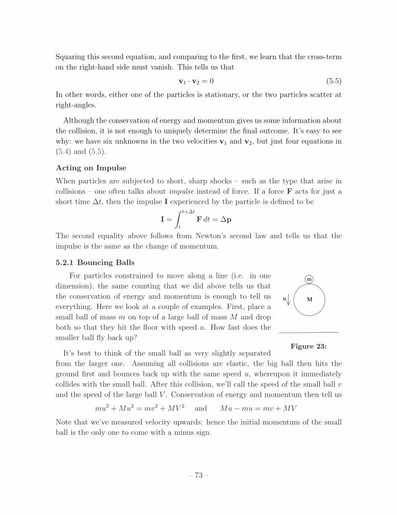
Squaring this second equation, and comparing to the first, we learn that the cross-term
on the right-hand side must vanish. This tells us that
v1 · v2 = 0 (5.5)
In other words, either one of the particles is stationary, or the two particles scatter at
right-angles.
Although the conservation of energy and momentum gives us some information about
the collision, it is not enough to uniquely determine the final outcome. It’s easy to see
why: we have six unknowns in the two velocities v1 and v2, but just four equations in
(5.4) and (5.5).
Acting on Impulse
When particles are subjected to short, sharp shocks – such as the type that arise in
collisions – one often talks about impulse instead of force. If a force F acts for just a
short time ∆t, then the impulse I experienced by the particle is defined to be
I =
∫ t+∆t
t
F dt = ∆p
The second equality above follows from Newton’s second law and tells us that the
impulse is the same as the change of momentum.
5.2.1 Bouncing Balls
For particles constrained to move along a line (i.e. in one
M
m
u
Figure 23:
dimension), the same counting that we did above tells us that
the conservation of energy and momentum is enough to tell us
everything. Here we look at a couple of examples. First, place a
small ball of mass m on top of a large ball of mass M and drop
both so that they hit the floor with speed u. How fast does the
smaller ball fly back up?
It’s best to think of the small ball as very slightly separated
from the larger one. Assuming all collisions are elastic, the big ball then hits the
ground first and bounces back up with the same speed u, whereupon it immediately
collides with the small ball. After this collision, we’ll call the speed of the small ball v
and the speed of the large ball V . Conservation of energy and momentum then tell us
mu2 +Mu2 = mv2 +MV 2 and Mu−mu = mv +MV
Note that we’ve measured velocity upwards: hence the initial momentum of the small
ball is the only one to come with a minus sign.
– 73 –

Just jumping in and solving these as simultaneous equations will lead to a quadratic
and some messy algebra. There’s a slightly slicker way. We write the two equations as
M(V − u)(V + u) = m(u− v)(u+ v) and M(u− V ) = m(v + u)
Dividing one by the other gives V +u = v−u. We can now use this and the momentum
conservation equation to eliminate V . We find
v =3M −mM +m
u
You can try this at home with a tennis ball and basketball. But trust the maths. It’s
telling you that the speed will be almost three times greater. This means that the
kinetic energy (and therefore the height reached by the tennis ball) will be almost nine
times greater. You have been warned!
5.2.2 More Bouncing Balls and the Digits of π
Here’s another example. The question seems a lit-
M m
Figure 24:
tle arbitrary, but the answer is quite extraordinary.
Consider two balls shown in the figure. The rightmost
ball has mass m. The leftmost ball is much heavier: it
has the rather strange mass M = 16×100N×m where
N is an integer.
We give the heavy ball a small kick so it rolls to the right. It collides elastically with
the light ball which then flies off towards the wall. The collision with the wall is also
elastic and the light ball bounces off with the same speed it arrived at, heading back
towards the heavy ball. The process keeps repeating: the light ball bounces off the
heavy one, bounces off the wall, and returns to collide yet again with the heavy ball.
Note that the total energy is conserved in all processes but the total momentum is not
conserved in the collision with the wall.
A priori, there are two possible outcomes of this. It may be that the heavy ball
moves all the way to the right where it too bounces off the wall (and, of course, the
light ball which is trapped between it and the wall). Or, it may be that the light ball
eventually collides enough times that the heavy ball turns around and starts moving
towards the left.
Which of these two possibilities occurs will be decided by the dynamics. Below,
we’ll see that it’s actually the latter scenario that takes place: the heavy ball does not
reach the wall. The question that we want to ask is: how many times, p(N), does the
heavy ball hit the lighter one before it turns around and starts heading in the opposite
direction?
– 74 –

The answer to this question is one of the most ridiculous things I’ve ever seen in
physics. It is5
p(N)− 1 = The first N + 1 digits of π
In other words, p(0)− 1 = 3, p(1)− 1 = 31, p(2)− 1 = 314, p(3)− 1 = 3141 and so on.
In case it’s not obvious, let me explain why you should also find this result ridiculous.
The number π is, of course, ubiquitous in physics. But this is very different from the
decimal expansion of the number. As the name suggests, the digits of π in a decimal
expansion have as much to do with biology as mathematics. But we subtly inserted
the relevant biological fact in the original question by insisting that the mass of the big
ball is M = 16× 102N ×m. This seemingly innocuous factor of 10 will prove to be the
reason that the expansion of π comes out in base 10.
Let’s now try to prove this unlikely result. Let un be the velocity of the heavy ball and
vn be the velocity of the light ball after the nth collision between them. Conservation
of energy and momentum tell us that
Mu2n+1 +mv2
n+1 = Mu2n +mv2
n
Mun+1 +mvn+1 = Mun −mvn
Rearranging these reveals some nice algebraic simplifications. Despite the quadratic
nature of the energy conservation equation, the relationship between the velocities
before and after is actually linear,(un+1
vn+1
)= A
(un
vn
)where the matrix A depends only on the ratio of masses which we denote as x = m/M
and is given by
A =1
1 + x
(1− x −2x
2 1− x
)Since we start with the only the heavy ball moving, (u0, v0) = (u0, 0). The velocities
after the nth collision between the balls are(un
vn
)= An
(u0
0
)(5.6)
5This is a variation of a problem first stated in the 2003 in the paper “Playing Pool with π” by
Gregory Galperin. The proof in this paper uses purely geometric techniques. I’m grateful to Joe
Minahan for help constructing this example, together with the proof below.
– 75 –

The smart way to compute the matrix An is to first diagonalise A .The eigenvalues of
A are easily computed to be e±iθ where
cos θ =1− x1 + x
Using this, we can write
An = S
(einθ 0
0 e−inθ
)S−1 with S =
1
1 + x
(i√x −i
√x
1 1
)(5.7)
and the velocities after the nth collision are given by(un
vn
)=
u0√x
(√x cosnθ
sinnθ
)We want to know how many collisions, p, it takes before the heavy ball starts moving
in the opposite direction. This occurs when cosnθ < 0, which means that p must obey
(p− 1)θ <π
2while pθ >
π
2
To get a feel for this, we’ll make an approximation. Since x = m/M , we can expand
cos θ ≈ 1 − 12θ2 ≈ 1 − 2x, which gives us θ ≈ 2
√x. Using our rather strange choice
of mass, x = 10−2N/16, so θ ≈ 10−N/2. If the corrections to this approximation are
unimportant, the number of collisions p is the largest integer such that (p−1)×10−N < π
while p× 10−N > π. The answer is
p(N)− 1 = [10Nπ]
which means the integer part of 10Nπ. This is the same thing as the first N + 1 digits
of π.
Finally, we should check whether the approximations that we made above are valid.
Is there some way the higher order terms that we neglected can change the answer?
Although we should check this, we won’t. Because it turns out to be quite tricky. If
you’re interested, some relevant details can be found in the original paper cited above.
5.3 Variable Mass Problems
Recall that the correct version of Newton’s second law is
p = F (5.8)
where p = mx is the momentum. This coincides with the more familiar mx = F only
when the mass of the object is unchanging. Here we will look at a few situations where
the mass actually does change. There are two canonical examples: things falling apart
and things gathering other stuff. We’ll treat them each in turn.
– 76 –

5.3.1 Rockets: Things Fall Apart
A rocket moves in a straight line with velocity v(t). The mass of the rocket, m(t),
changes with time because it propels itself forward by spitting out fuel behind. Suppose
that the fuel is ejected at a speed u relative to the rocket. Our goal is to figure out how
the speed of the rocket changes over time.
You might think that we should just plug this into Newton’s second law (5.8) to get
“d(mv)/dt = F”. But this isn’t quite right. The equation (5.8) refers to the momentum
of the entire system, which in this case includes the rocket and the ejected fuel. And
we need to take both into account.
To proceed, it’s best to go back to first principles
time t+ tδ
m(t+ t)δ
m(t)−m(t+ t)δ
m(t)
time t
Figure 25:
and work infinitesimally. At time t, the momentum of the
rocket is
p(t) = m(t)v(t)
After a short interval δt, this momentum is split between
the momentum of the rocket and the momentum of the
recently ejected fuel,
p(t+ δt) = procket(t+ δt) + pfuel(t+ δt)
The momentum of the rocket at this later time is given by
procket(t+ δt) = m(t+ δt)v(t+ δt)
≈(m(t) +
dm
dtδt
)(v(t) +
dv
dtδt
)≈ m(t)v(t) +
(vdm
dt+m
dv
dt
)δt+O(δt2)
where we’ve Taylor expanded the mass and velocity and kept terms up to order δt.
Similarly, the momentum of the fuel ejected between time t and t+ δt is
pfuel(t+ δt) = [m(t)−m(t+ δt)] [v(t)− u]
≈ −dmdtδt [v(t)− u] +O(δt2)
Notice that the speed of the fuel is v−u; this is because the fuel has speed u relative to
the rocket. In fact, there’s a small subtlety here. Does the fuel travel at velocity v(t)−uor v(t+ δt)− u or some average of the two? In fact, it doesn’t matter. The difference
– 77 –

only shows up at order δt2 and doesn’t affect our final answer. Adding together these
two momenta, we have the result
p(t+ δt) = p(t) +
(m(t)
dv
dt+ u
dm
dt
)δt+O(δt2) (5.9)
At this stage, we can use Newton’s second law in the form (5.8) which, using the
definition of the derivative, is given by
p(t+ δt)− p(t)δt
= F
Comparing this to (5.9), we arrive at the Tsiolkovsky rocket equation
m(t)dv
dt+ u
dm
dt= F (5.10)
Apparently, this equation was first derived only in 1903.
An Example: A Free Rocket in Space
Let’s solve the rocket equation when there is no external force, F = 0. We can write it
as
dv
dt= − u
m
dm
dt
which can be trivially integrated to give
v(t) = v0 + u log
(m0
m(t)
)Here we have chosen the rocket to have speed v0 when its mass is m0. We see that
burning rocket fuel will only increase your speed logarithmically. If we further assume
that the rocket burns fuel at a constant rate,
dm
dt= −α
then we have m(t) = m0 − αt. (Note that α > 0 means that dm/dt < 0 as it should
be). In this case, the velocity of the rocket is
v(t) = v0 − u log
(1− αt
m0
)Notice that this solution only makes sense for times t < m0/α. This is because at time
t = m0α, all of the fuel runs out which, in our somewhat silly model, means that the
rocket has disappeared entirely. For these times t < m0/α, we can integrate once more
to get the position
x = v0t+um0
α
[(1− αt
m0
)log
(1− αt
m0
)+αt
m0
]
– 78 –

Another Example: A Rocket with Linear Drag
Here’s a slightly more involved example. The initial mass of the rocket is m0 and we will
still burn fuel at a constant rate, so m = −α. But now the rocket is subject to linear
drag, F = −γv, presumably because it has encountered some sticky alien intergalactic
golden syrup or something. If the rocket starts from rest, how fast is it going after it
has burned one half of its mass as fuel?
With linear drag, the rocket equation (5.10) becomes
mv + um = −γv (5.11)
We can already get a feel for what’s going on by looking at this equation. Since m = −α,
rearranging we get
mv = αu− γv
This means that we will continue to accelerate through the sticky alien goo if we’re
travelling slowly and burning fuel fast enough so that αu > γv. But as our speed
approaches v = αu/γ, the acceleration slows down and we expect this to be the limiting
velocity. However, if we were travelling too fast to begin with, so γv > αu, then we
will slow down until we again hit the limiting speed v = αu/γ.
Let’s now look in more detail at the solution. We could solve the rocket equation
(5.11) to get v(t), but since the question doesn’t ask about velocity as a function of
time, we’ll be much better off thinking of velocity as a function of mass: v = v(m).
Then
v =dv
dmm = −α dv
dm
Using this, the rocket equation becomes
−αm dv
dm− αu = −γv
This can be happily integrated using a few basic steps,
dv
dm=γv − αuαm
⇒∫
dv
γv − αu=
∫dm
αm
Before integrating, we need to decide whether the denominator on the left-hand side
is positive or negative. (Because integrating will give us a log and the argument of log
– 79 –
has to be positive). Because we stated above that the rocket starts from rest, we have
γv < αu meaning that the left-hand side is negative. Integrating then gives
1
γlog
(αu− γvαu
)=
1
αlog
(m
m0
)Here the denominators that we introduced in the argument of both logs are there on
dimensional grounds. (Remember that the argument of log has to be dimensionless).
The factor of m0 is an integration constant; the factor of αu tells us that the velocity
vanishes when m = m0. Rearranging, we get the final answer
v =αu
γ
(1−
(m
m0
)γ/α)
We see that the behaviour is in agreement with our discussion after (5.11); as m de-
creases, v increases to towards the limiting velocity v = αu/γ. But it never reaches this
velocity until all the mass of the rocket is burnt as fuel. In particular, we can answer
the question posed at the beginning simply by setting m = m0/2.
5.3.2 Avalanches: Stuff Gathering Other Stuff
It’s somewhat more natural to come up with examples where things fall apart and
the mass decreases. But, for completeness, let’s discuss a situation where the mass
increases: avalanches. I should confess up front that avalanches are very poorly under-
stood and the model below holds no claim to realism.
We’ll denote the mass of snow moving in the avalanche as m(t). We’ll further assume
that all the snow moves down the hill at the same speed v(t), picking up extra snow as
it goes. We can use the rocket equation (5.10), with u = v since the the snow lying on
the ground which is picked up has speed v relative to the avalanche. Ignoring friction,
but including the force due to gravity, the rocket equation becomes
mdv
dt+ v
dm
dt= mg sin θ
where θ is the angle that the slope makes with the ground. Because the snow lying on
the ground had no momentum, we do get the naive equation that comes from simply
plugging the momentum of the avalanche into (5.8)
d
dt(mv) = mg sin θ
– 80 –
Suppose that the snow has density ρ, height h and all of it is picked up as the avalanche
passes over. Then after the avalanche has moved a distance x down the slope, it has
picked up a mass m(t) = ρhx(t). The equation of motion is
d
dt(ρhxv) = ρhxg sin θ
At this point, it is best to think of velocity as a function of position: v = v(x). Then
we can write d/dt = v d/dx so
vd
dx(xv) = xg sin θ
This is again easily integrated in a few standard manoeuvres. If we first multiply both
sides by x, we have
xvd
dx(xv) = x2g sin θ ⇒ 1
2(xv)2 =
1
3x3g sin θ
where we’ve set the integration constant to zero so that v = 0 when we start at x = 0.
Rearranging now gives the speed as a function of position,
v =
√2
3xg sin θ
If we integrate this once more, we get
x =1
6gt2 sin θ
where we again set the integration constant to zero by assuming that x = 0 when t = 0.
It’s worth mentioning that this is a factor of 1/3 smaller than the result we get for an
object that doesn’t gather mass as it goes which, taken at face value, suggests that
you should be able to outrun an avalanche, at least if you didn’t have to worry about
friction. Personally, I wouldn’t bet on it.
5.4 Rigid Bodies
So far, we’ve only discussed “particles”, objects with no extended size. But what
happens to more complicated objects that can twist and turn as they move? The
simplest example is a rigid body. This is a collection of N particles, constrained so that
the relative distance between any two points, i and j, is fixed:
|xi − xj| = fixed
A rigid body can undergo only two types of motion: its centre of mass can move; and it
can rotate. We’ll start by considering just the rotations. In Section 5.4.5, we’ll combine
the rotations with the centre of mass motion.
– 81 –

5.4.1 Angular Velocity
We fix some point in the rigid body and consider
y
xθ
z,ω
φ
r
d
Figure 26:
rotation about this point. To describe these rotations,
we need the concept of angular velocity. We’ll begin by
considering a single particle which is rotating around the
z-axis, as shown in the figure. The position and velocity
of the particle are given by
x = (d cos θ, d sin θ, z) ⇒ x = (−θd sin θ, θd cos θ, 0)
We can write this by introducing a new vector ω = θz,
x = ω × x
The vector ω is called the angular velocity. In general we can write ω = ωn. Here
the magnitude, ω = |θ| is the angular speed of rotation, while the unit vector n points
along the axis of rotation, defined in a right-handed sense. (Curl the fingers of your
right hand in the direction of rotation: your thumb points in the direction of ω).
The speed of the particle is then given by
v = |x| = rω sinφ = dω
where
d = |n× x| = r sinφ
is the perpendicular distance to the axis of rotation as shown in the figure. Finally, we
will also need an expression for the kinetic energy of this particle as it rotates about
the axis n through the origin; it is
T =1
2mx · x =
1
2m(ω × x) · (ω × x) =
1
2md2ω2 (5.12)
5.4.2 The Moment of Inertia
Now let’s return to our main theme and look at a collection of N particles which make
up a rigid body. The fact that the object is rigid means that all particles rotate with
the same angular velocity,
xi = ω × xi
– 82 –

This ensures that the relative distance between points remains fixed as it should:
d
dt|xi − xj|2 = 2(xi − xj) · (xi − xj)
= 2[ω × (xi − xj)] · (xi − xj) = 0
We can write the kinetic energy for a rigid body as
T =1
2
∑i
mixi · xi =1
2Iω2
where
I ≡N∑i=1
mid2i
is the moment of inertia. Notice the similarity between the rotational kinetic energy12Iω2 and the translational kinetic energy 1
2Mv2. The moment of inertia is to rotations
what the mass is to translations. The bigger I, the more energy you need to supply to
the body to make it spin.
The moment of inertia also plays a role in the angular momentum of the rigid body.
We have
L =∑i
mixi × xi =∑i
mixi × (ω × xi)
If we write ω = ωn, for a unit vector n, then the magnitude of the angular momentum
in the direction of ω is
L · n = ω∑i
mi
(xi × (n× xi)
)· n
= ω∑i
mi(xi × n) · (xi × n)
= Iω
We saw earlier in (5.2) that acting with a torque τ changes the angular momentum:
L = τ . For a rigid body, we learn that if the torque is in the same direction as the
angular velocity, so τ = τ n, then the change in the angular velocity is simply
Iω = τ
– 83 –

Calculating the Moment of Inertia
It’s often useful to treat rigid bodies as continuous objects. This means that we replace
the discrete particle masses mi with a continuous density distribution ρ(x). In this
course, we will nearly always be interested in uniform objects for which the density
ρ is constant. (Although a spatially dependent ρ doesn’t add any more conceptual
difficulties). The total mass of the body is then given by a volume integral
M =
∫ρ(x) dV
and the moment of inertia is
I =
∫ρ(x)x2
⊥ dV =
∫ρ(x) (x sinφ)2 dV
where x⊥ = x sinφ is the perpendicular distance from the point x to the axis of rotation.
Let’s look at some simple examples.
A Circular Hoop
A uniform hoop has mass M and radius a. Take the axis of rotation to pass through the
centre, perpendicular to the plane of the hoop. This is, perhaps the simplest example,
because all points of the hoop lie at the same distance, a, from the centre. The moment
of inertia is simply
I = Ma2
A Rod
A rod has length l, mass M and uniform density ρ = M/l (strictly this is mass per
unit length rather than mass per volume). The moment of inertia about an axis per-
pendicular to the rod, passing through the end point is
I =
∫ l
0
ρx2 dx =1
3ρl3 =
1
3Ml2 (5.13)
A Disc
A uniform disc has radius a and mass M = πρa2. Two dimensional objects, such as
the disc, are sometimes referred to as laminas. This time we’ll look at two different
axes of rotation.
– 84 –

We start with an axis of rotation through the centre, perpendicular to the plane
of the disc. We can compute the moment of inertia using plane polar coordinates.
Recall that we need to include a Jacobian factor of r, so that the infinitesimal area is
dA = rdrdθ. The moment of inertia is then
I =
∫ a
0
∫ 2π
0
ρr2 rdrdθ =1
4ρ (2πa4) =
1
2Ma2
We can also look at an axis rotation that passes through the centre of the disc but, this
time, lies within the plane of the disc. We’ll choose polar coordinates so that θ = 0 lies
along the axis of rotation. Then the point with coordinates (r, θ) lies a distance r sin θ
away from the axis of rotation. The moment of inertia is now
I =
∫ a
0
∫ 2π
0
ρ(r sin θ)2 rdrdθ =1
4Ma2
In fact, these two calculations illustrate a general fact about laminas. If we take the z
axis to lie perpendicular to the plane of the lamina, then the moments of inertia about
the x and y-axes are Ix =∫ρy2 dA and Iy =
∫ρx2 dA. Meanwhile, the distance of any
point to the z-axis is r =√x2 + y2, so the moment of inertia about the z-axis is
Iz =
∫ρ(x2 + y2) dA = Ix + Iy
This is known as the perpendicular axis theorem
A Sphere
A uniform sphere has radius a and mass M = 43πρa3. We pick spherical polar coor-
dinates with the axis θ = 0 pointing along the axis of rotation which passes through
the centre of the sphere. A point with coordinates (r, θ, φ) has distance r sin θ from the
axis of rotation. We also have the Jacobian factor r2 sin θ, so that the volume element
is dV = r2 sin θdrdθdφ with θ ∈ [0, π) and φ ∈ [0, 2π). The moment of inertia is
I =
∫ a
0
∫ π
0
∫ 2π
0
ρ(r sin θ)2 r2 sin θ drdθdφ =8
15πρa5 =
2
5Ma2
5.4.3 Parallel Axis Theorem
A rigid body has mass M and moment of inertia ICoM about an axis which passes
through its centre of mass. Let I be the moment of inertia about a parallel axis that
lies a distance h away. Then
I = ICoM +Mh2
This is the parallel axis theorem.
– 85 –
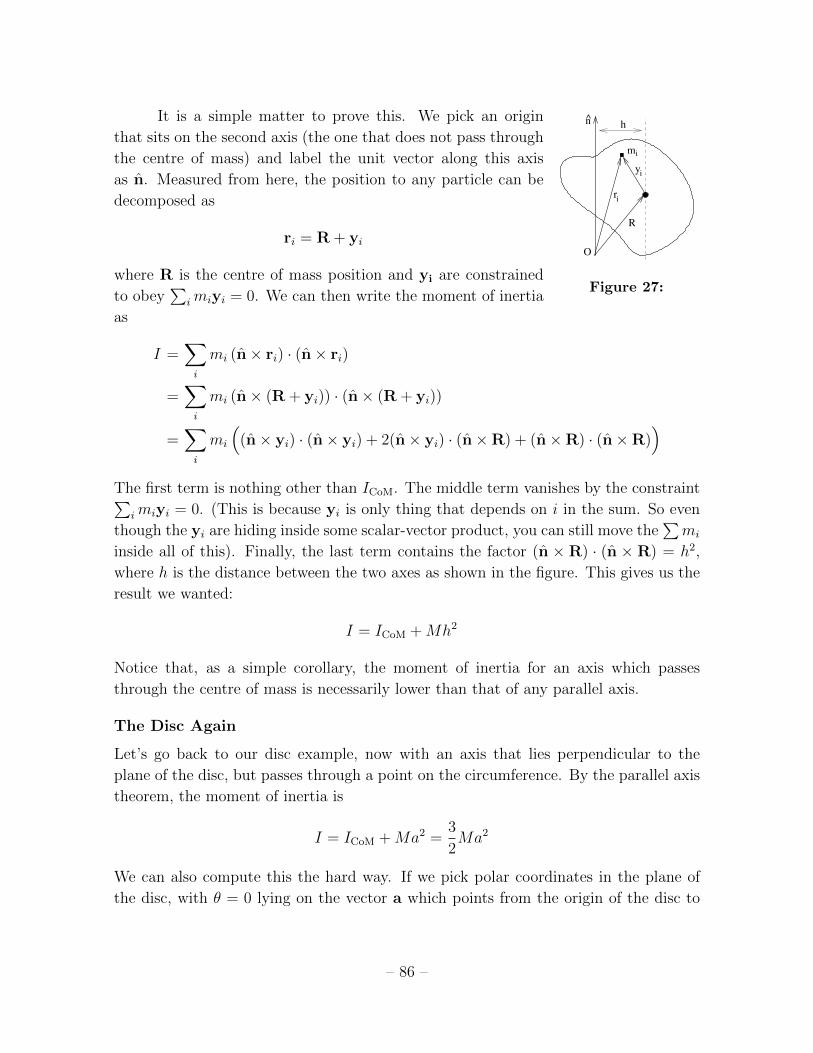
It is a simple matter to prove this. We pick an origin
mi
ri
yi
R
O
hn
Figure 27:
that sits on the second axis (the one that does not pass through
the centre of mass) and label the unit vector along this axis
as n. Measured from here, the position to any particle can be
decomposed as
ri = R + yi
where R is the centre of mass position and yi are constrained
to obey∑
imiyi = 0. We can then write the moment of inertia
as
I =∑i
mi (n× ri) · (n× ri)
=∑i
mi (n× (R + yi)) · (n× (R + yi))
=∑i
mi
((n× yi) · (n× yi) + 2(n× yi) · (n×R) + (n×R) · (n×R)
)The first term is nothing other than ICoM. The middle term vanishes by the constraint∑
imiyi = 0. (This is because yi is only thing that depends on i in the sum. So even
though the yi are hiding inside some scalar-vector product, you can still move the∑mi
inside all of this). Finally, the last term contains the factor (n × R) · (n × R) = h2,
where h is the distance between the two axes as shown in the figure. This gives us the
result we wanted:
I = ICoM +Mh2
Notice that, as a simple corollary, the moment of inertia for an axis which passes
through the centre of mass is necessarily lower than that of any parallel axis.
The Disc Again
Let’s go back to our disc example, now with an axis that lies perpendicular to the
plane of the disc, but passes through a point on the circumference. By the parallel axis
theorem, the moment of inertia is
I = ICoM +Ma2 =3
2Ma2
We can also compute this the hard way. If we pick polar coordinates in the plane of
the disc, with θ = 0 lying on the vector a which points from the origin of the disc to
– 86 –

the axis of rotation. Then the distance from the axis, d, of a point r in the disc is given
by
d2 = (r− a)2 = r2 + a2 − 2r · a = r2 + a2 − 2ar cos θ
From this we can compute the moment of inertia
I =
∫ a
0
∫ 2π
0
ρ(r2 + a2 − 2ar cos θ) rdr dθ =3
2Ma2
in agreement with our result using the parallel axis theorem.
5.4.4 The Inertia Tensor
The moment of inertia is not inherent to the rigid body itself; it also depends on the
axis about which we rotate. There is a more refined quantity which is a property only
of the rigid body and contains the necessary information to compute the moment of
inertia about any given axis. This is a 3× 3 matrix, known as the inertia tensor I.
We can already see the inertia tensor sitting in our expression for the kinetic energy
of a rotating object, which we write as
T =1
2
∑i
mi(ω × xi) · (ω × xi)
=1
2
∑i
mi
((ω · ω)(xi · xi)− (xi · ω)2
)=
1
2ωTIω
where the components of the inertia tensor are expressed in terms of the components
(xi)a, a = 1, 2, 3 of the position vectors as
Iab =∑i
mi
((xi · xi)δab − (xi)a(xi)b
)The moment of inertia about an axis n is encoded in the inertia tensor as
I = nTI n
There are many further interesting properties of the inertia tensor. Perhaps the most
important is that it relates the angular momentum with the angular velocity. It is not
hard to show
L = Iω
– 87 –
In particular, this means that the angular momentum does not necessarily lie in the
same direction as the angular velocity. (This is only true if the object is spinning about
an eigenvector of the inertia tensor). This is responsible for many of the weird and
wobbly properties of spinning objects. However, a much fuller discussion will have to
wait until the next Classical Dynamics course6.
5.4.5 Motion of Rigid Bodies
So far we have just considered the rotation of a rigid body about some point. Now
let’s set it free and allow it to move. The most general motion of a rigid body can be
described by its centre of mass following some trajectory, R(t), together with a rotation
about the centre of mass. We use our usual notation where the position of any particle
in the rigid body is written as
ri = R + yi ⇒ ri = R + yi
If the body rotates with angular velocity ω around the centre of mass, we have yi =
ω × yi, which means that we can write
ri = R + ω × (ri −R) (5.14)
The kinetic energy of the rigid body follows from the general calculation (5.3), together
with our result (5.12). These give
T =1
2MR · R +
1
2
∑i
miyi · yi
=1
2MR · R +
1
2Iω2 (5.15)
(Recall, that this calculation needs us to work with the centre of mass R to ensure that
the cross-terms R · yi drop out in the first line above).
Motion with Rotation about A Different Point
It is certainly most natural to split the motion into the centre of mass trajectory R(t)
together with rotation about the centre of mass. With this choice, Newton’s second
law (5.1) ensures that R(t) is dictated only by external forces. Moreover, the kinetic
energy splits nicely into translational and rotational energies (5.15). But nothing tells
us that we have to describe an object in this way. We could, instead, decide that it’s
better to think of the motion in terms of some other point Q (say the tip of the nose
of dead, rigid cat), together with rotation about Q.
6See section 3 of the lectures notes at http://www.damtp.cam.ac.uk/user/tong/dynamics.html
– 88 –

We can derive an expression for such motion using our results above. Let’s start by
picking ri = Q in (5.14). This tells us
Q = R + ω × (Q−R)
If we substitute this back into (5.14), we can eliminate R to get an expression for the
motion of any point ri about Q,
ri = Q + ω × (ri −Q)
There’s something a little surprising about this: the angular velocity ω about any point
is the same.
An Example: Roll, Don’t Slip
A common example of rigid body motion is an
A
P
θ
θ/2
a
Figure 28:
object which rolls along the ground. Let’s look
at a hoop of radius a as shown in the figure. In
this case, the translational speed and the angular
speed are related. This comes about if we insist
that there is no slipping between the hoop and
the ground — a requirement that is usually, quite
reasonably, called the no-slip condition.
Consider the point A of the hoop which, at a
given instance, is in contact with the ground. The no slip condition is the statement
that the point A is instantaneously at rest. In other words, it has no speed relative
to the ground. If we denote the angular speed of the hoop as θ, the no-slip condition
means that the horizontal speed v of the origin is
v = aθ (5.16)
What, however, is the speed of different point, P on the circumference? Clearly when
θ = 0, so P sits at the top of the hoop, the horizontal speed is aθ with respect to centre,
resulting in a total horizontal speed of 2aθ.
To compute the speed of a general point P , it’s best to think about the hoop as
rotating about A. From the argument above, we know that the angular speed about
A is also θ. But the distance AP = 2a cos(θ/2), which means that the speed v of the
point P relative to A (which is the same as relative to the ground) is
v = 2aθ cos (θ/2)
We check that this gives the right answer when P is at the top and bottom of the hoop:
θ = 0 and θ = π gives v = 2aθ and v = 0 respectively, as it should.
– 89 –

Note that the velocity of the point P does not lie tangent to the circle. That would
only be the case if the hoop was rotating while staying fixed. Instead the velocity of
point P is at right-angles to the line AP . This reflects the fact that the point P is
rotating about the origin, but also moving forwards as the hoop moves.
Finally, a quick comment: despite the presence of friction, this is one example where
we can still use energy conservation. This is because the point of the wheel that is in
contact with the ground is at rest, which means that friction acting on this point does
no work. Instead, the only role of friction is to impose the no-slip condition. We’ll see
an example of this motion which can be solved using energy conservation shortly.
Another Example: A Swinging Rod
Until now, a “pendulum” has always consisted of a mass sitting at the end
θ
mg
L/2
Figure 29:
of a light rod, where light means effectively massless. Let’s now look at
an example where the rod itself has mass m.
This is a case where the most natural description of the rotation is
around the pivot, rather than around the centre of mass. We already
calculated the moment of inertia I for a rod of length L which pivots
about its end point (5.13): I = 13mL2. With the angular speed ω = θ, the
kinetic energy can be written as
T =1
2Iθ2
Alternatively, we could also look at this as motion of the centre of mass, together with
rotation around the centre of mass. As we saw above, the angular speed about the
centre of mass remains θ: it is the same as the angular speed about the pivot. The
speed of the centre of mass is v = (L/2)θ and the kinetic energy splits in the form
(5.15)
T = Translational K.E. + Rotational K.E. =1
2m
(L
2θ
)2
+1
2ICoMθ
2
But, by the parallel axis theorem, we know that I = ICoM + m(L/2)2 which happily
means that the kinetic energies computed in these two different ways coincide.
To derive the equation of motion of the pendulum, it’s perhaps easiest to first get
the energy. The centre of mass of the pendulum sits at a distance −(L/2) cos θ below
the pivot. So combining the kinetic and gravitational energies, we have
E =1
2Iθ2 −mgL
2cos θ
– 90 –

Differentiating with respect to time, we get the equation of motion
Iθ = −mgL2
sin θ
We can compare this with our earlier treatment of a pendulum where all the mass sits
at the end of the length l. In that case, the equation is (2.9). We see that the equations
of motion agree if set l = 2I/Lm = 2L/3.
Yet Another Example: A Rolling Disc
A disc of mass M and radius a rolls down a slope without slipping. The plane of the
disc is vertical. The moment of inertia of the disc about an axis which passes through
the centre, perpendicular to the plane of the disc, is I. (We already know from our
earlier calculation that I = 12Ma2, but we’ll leave it general for now).
We’ll denote the speed of the disc down the slope as v andω
v
a
α
Figure 30:
the angular speed of the disc as ω. (From the picture and the
right-hand rule, we see that the angular velocity ω is a vector
point out of the page). As in (5.16), the no-slip condition gives
us the relation
v = aω
To understand the motion of the disc, it is simplest to work
with the energy. This is allowed since, as we mentioned before, when friction imposes
the no-slip condition it does no work. We’ve seen a number of times — e.g. in (5.15) —
that the kinetic energy splits into the translational kinetic energy of the centre of mass,
together with the rotational kinetic energy about the centre of mass. In the present
case, this means
T =1
2Mv2 +
1
2Iω2 =
1
2
(I
a2+M
)v2
Including the gravitational potential energy, we have
E =1
2
(I
a2+M
)x2 −Mgx sinα
where x measures the progress of the disc down the slope, so x = v. From this we can
derive the equation of motion simply by taking the time derivative. We have(I
a2+M
)x = Mg sinα
– 91 –
We learn that while the overall mass M drops out of the calculation (recall that I is
proportional to M), the moment of inertia I does not. The larger the moment of inertia
I of an object, the slower its progress down the slope. This is because the gravitational
potential energy is converted into both translational and rotational kinetic energy. But
only the former affects how fast the object makes it down. The upshot of this is that
if you take a hollow cylinder and a solid cylinder with equal diameter, the solid one –
with smaller moment of inertia – will make it down the slope more quickly.
– 92 –

6. Non-Inertial Frames
We stated, long ago, that inertial frames provide the setting for Newtonian mechanics.
But what if you, one day, find yourself in a frame that is not inertial? For example,
suppose that every 24 hours you happen to spin around an axis which is 2500 miles
away. What would you feel? Or what if every year you spin around an axis 36 million
miles away? Would that have any effect on your everyday life?
In this section we will discuss what Newton’s equations of motion look like in non-
inertial frames. Just as there are many ways that an animal can be not a dog, so
there are many ways in which a reference frame can be non-inertial. Here we will just
consider one type: reference frames that rotate. We’ll start with some basic concepts.
6.1 Rotating Frames
Let’s start with the inertial frame S drawn in the figurez=z
x
y
x
y
θ
Figure 31:
with coordinate axes x, y and z. Our goal is to understand
the motion of particles as seen in a non-inertial frame S ′,
with axes x′, y′ and z′, which is rotating with respect to S.
We’ll denote the angle between the x-axis of S and the x′-
axis of S ′ as θ. Since S ′ is rotating, we clearly have θ = θ(t)
and θ 6= 0.
Our first task is to find a way to describe the rotation of
the axes. For this, we can use the angular velocity vector ω
that we introduced in the last section to describe the motion of particles. Consider a
particle that is sitting stationary in the S ′ frame. Then, from the perspective of frame
S it will appear to be moving with velocity
r = ω × r
where, in the present case, ω = θz. Recall that in general, |ω| = θ is the angular speed,
while the direction of ω is the axis of rotation, defined in a right-handed sense.
We can extend this description of the rotation of the axes of S ′ themselves. Let e ′i ,
i = 1, 2, 3 be the unit vectors that point along the x′, y′ and z′ directions of S ′. Then
these also rotate with velocity
e ′i = ω × e ′i
This will be the main formula that will allow us to understand motion in rotating
frames.
– 93 –

6.1.1 Velocity and Acceleration in a Rotating Frame
Consider now a particle which is no longer stuck in the S ′ frame, but moves on some
trajectory. We can measure the position of the particle in the inertial frame S, where,
using the summation convention, we write
r = riei
Here the unit vectors ei, with i = 1, 2, 3 point along the axes of S. Alternatively, we
can measure the position of the particle in frame S ′, where the position is
r = r′ie′i
Note that the position vector r is the same in both of these expressions: but the
coordinates ri and r′i differ because they are measured with respect to different axes.
Now, we can compute an expression for the velocity of the particle. In frame S, it is
simply
r = riei (6.1)
because the axes ei do not change with time. However, in the rotating frame S ′, the
velocity of the particle is
r = r′ie′i + r′ie
′i
= r′ie′i + r′iω × e ′i
= r′ie′i + ω × r (6.2)
We’ll introduce a slightly novel notation to help highlight the physics hiding in these
two equations. We write the velocity of the particle as seen by an observer in frame S
as (dr
dt
)S
= riei
Similarly, the velocity as seen by an observer in frame S ′ is just(dr
dt
)S′
= r′ie′i
From equations (6.1) and (6.2), we see that the two observers measure different veloc-
ities, (dr
dt
)S
=
(dr
dt
)S′
+ ω × r (6.3)
This is not completely surprising: the difference is just the relative velocity of the two
frames.
– 94 –

What about acceleration? We can play the same game. In frame S, we have
r = riei
while in frame S ′, the expression is a little more complicated. Differentiating (6.2) once
more, we have
r = r′ie′i + r′iei
′ + r′iω × e ′i + r′iω × e ′i + r′iω × ei′
= r′ie′i + 2r′iω × e ′i + ω × r + r′iω × (ω × ei
′)
As with velocities, the acceleration seen by the observer in S is riei while the accel-
eration seen by the observer in S ′ is r′ie′i . Equating the two equations above gives
us (d2r
dt2
)S
=
(d2r
dt2
)S′
+ 2ω ×(dr
dt
)S′
+ ω × r + ω × (ω × r) (6.4)
This equation contains the key to understanding the motion of particles in a rotating
frame.
6.2 Newton’s Equation of Motion in a Rotating Frame
With the hard work behind us, let’s see how a person sitting in the rotating frame S ′
would see Newton’s law of motion. We know that in the inertial frame S, we have
m
(d2r
dt2
)S
= F
So, using (6.4), in frame S ′, we have
m
(d2r
dt2
)S′
= F− 2mω ×(dr
dt
)S′−mω × r−mω × (ω × r) (6.5)
In other words, to explain the motion of a particle an observer in S ′ must invoke the
existence of three further terms on the right-hand side of Newton’s equation. These are
called fictitious forces. Viewed from S ′, a free particle doesn’t travel in a straight line
and these fictitious forces are necessary to explain this departure from uniform motion.
In the rest of this section, we will see several examples of this.
The −2mω× r term in (6.5) is the Coriolis force; the −mω× (ω× r) term is called
the centrifugal force; the −mω × r term is called the Euler force.
– 95 –

The most familiar non-inertial frame is
Figure 32: xkcd.com
the room you are sitting in. It rotates once per
day around the north-south axis of the Earth.
It further rotates once a year about the Sun
which, in turn, rotates about the centre of the
galaxy. From these time scales, we can easily
compute ω = |ω|.
The radius of the Earth is REarth ≈ 6 ×10³ km. The Earth rotates with angular fre-
quency
ωrot =2π
1 day≈ 7× 10⁻⁵ s−1
The distance from the Earth to the Sun is ae ≈2×10⁸ km. The angular frequency of the orbit
is
ωorb =2π
1 year≈ 2× 10⁻⁷ s−1
It should come as no surprise to learn that
ωrot/ωorb = Torb/Trot ≈ 365.
In what follows, we will see the effect of the centrifugal and Coriolis forces on our
daily lives. We will not discuss the Euler force, which arises only when the speed of
the rotation changes with time. Although this plays a role in various funfair rides, it’s
not important in the frame of the Earth. (The angular velocity of the Earth’s rotation
does, in fact, have a small, but non-vanishing, ω due to the precession and nutation of
the Earth’s rotational axis. However, it is tiny, with ω ω2 and, as far as I know, the
resulting Euler force has no consequence).
Inertial vs Gravitational Mass Revisited
Notice that all the fictitious forces are proportional to the inertial mass m. There is
no mystery here: it’s because they all originated from the “ma” side of “F=ma” rather
than “F” side. But, as we mentioned in Section 2, experimentally the gravitational
force also appears to be proportional to the inertial mass. Is this evidence that gravity
too is a fictitious force? In fact it is. Einstein’s theory of general relativity recasts
gravity as the fictitious force that we experience due to the curvature of space and
time.
– 96 –
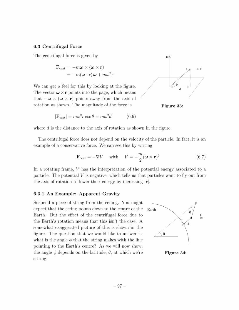
6.3 Centrifugal Force
The centrifugal force is given by ω
d
x F
θ
Figure 33:
Fcent = −mω × (ω × r)
= −m(ω · r)ω +mω2r
We can get a feel for this by looking at the figure.
The vector ω× r points into the page, which means
that −ω × (ω × r) points away from the axis of
rotation as shown. The magnitude of the force is
|Fcent| = mω2r cos θ = mω2d (6.6)
where d is the distance to the axis of rotation as shown in the figure.
The centrifugal force does not depend on the velocity of the particle. In fact, it is an
example of a conservative force. We can see this by writing
Fcent = −∇V with V = −m2
(ω × r)2 (6.7)
In a rotating frame, V has the interpretation of the potential energy associated to a
particle. The potential V is negative, which tells us that particles want to fly out from
the axis of rotation to lower their energy by increasing |r|.
6.3.1 An Example: Apparent Gravity
Suspend a piece of string from the ceiling. You might
Earthφ
θ
F
g
Figure 34:
expect that the string points down to the centre of the
Earth. But the effect of the centrifugal force due to
the Earth’s rotation means that this isn’t the case. A
somewhat exaggerated picture of this is shown in the
figure. The question that we would like to answer is:
what is the angle φ that the string makes with the line
pointing to the Earth’s centre? As we will now show,
the angle φ depends on the latitude, θ, at which we’re
sitting.
– 97 –

The effective acceleration, due to the combination of gravity and the centrifugal force,
is
geff = g − ω × (ω × r)
It is useful to resolve this acceleration in the radial and southerly θ^
r
Earth
^
Figure 35:
directions by using the unit vectors r and θ. The centrifugal force F
is resolved as
F = |F| cos θ r− |F| sin θ θ= mω2r cos2 θ r−mω2r cos θ sin θ θ
where, in the second line, we have used the magnitude of the cen-
trifugal force computed in (6.6). Notice that, at the pole θ = π/2
and the centrifugal forces vanishes as expected. This gives the effective acceleration
geff = −gr− ω × (ω × r) = (−g + ω2R cos2 θ)r− ω2R cos θ sin θ θ
where R is the radius of the Earth.
The force mgeff must be balanced by the tension T in the string. This too can be
resolved as
T = T cosφ r + T sinφ θ
In equilibrium, we need mgeff +T = 0, which allows us to eliminate T to get an equation
relating φ to the latitude θ,
tanφ =ω2R cos θ sin θ
g − ω2R cos2 θ
This is the answer we wanted. Let’s see at what latitude the angle φ is largest. If
we compute d(tanφ)/dθ, we find a fairly complicated expression. However, if we take
int account the fact that ω2R ≈ 3 × 10⁻² ms−2 g then we can neglect the term in
which we differentiate the denominator. We learn that the maximum departure from
the vertical occurs more or less when d(cos θ sin θ)/dθ = 0. Or, in other words, at a
latitude of θ ≈ 45. However, even at this point the deflection from the vertical is tiny:
an order of magnitude gives φ ≈ 10−4.
– 98 –

When we sit at the equator, with θ = 0, then φ = 0 and the string hangs directly
towards the centre of the Earth. However, gravity is somewhat weaker due to the
centrifugal force. We have
geff |equator = g − ω2R
Based on this, we expect geff − g ≈ 3× 10⁻² ms−2 at the equator. In fact, the experi-
mental result is more like 5× 10⁻² ms−2. The reason for this discrepancy can also be
traced to the centrifugal force which means that the Earth is not spherical, but rather
bulges near the equator.
A Rotating Bucket
Fill a bucket with water and spin it. The surface of the water ω
r
Figure 36:
will form a concave shape like that shown in the figure. What
is the shape?
We assume that the water spins with the bucket. The poten-
tial energy of a water molecule then has two contributions: one
from gravity and the other due to the centrifugal force given
in (6.7)
Vwater = mgz − 1
2mω2r2
Now we use a somewhat slick physics argument. Consider a
water molecule on the surface of the fluid. If it could lower its energy by moving along
the surface, then it would. But we’re looking for the equilibrium shape of the surface,
which means that each point on the surface must have equal potential energy. This
means that the shape of the surface is a parabola, governed by the equation
z =ω2r2
2g+ constant
6.4 Coriolis Force
The Coriolis force is given by
Fcor = −2mω × v
where, from (6.5), we see that v = (dr/dt)S′ is the velocity of the particle measured
in the rotating frame S ′. The force is velocity dependent: it is only felt by moving
particles. Moreover, it is independent on the position.
– 99 –

6.4.1 Particles, Baths and Hurricanes
The mathematical form of the Coriolis force is identical to the
Figure 37:
Lorentz force (2.19) describing a particle moving in a magnetic
field. This means we already know what the effect of the
Coriolis force will be: it makes moving particles turn in circles.
We can easily check that this is indeed the case. Consider
a particle moving on a spinning plane as shown in the figure,
where ω is coming out of the page. In the diagram we have
drawn various particle velocities, together with the Coriolis force experienced by the
particle. We see that the effect of the Coriolis force is that a free particle travelling on
the plane will move in a clockwise direction.
There is a similar force — at least in principle — when you pull the plug from your
bathroom sink. But here there’s a subtle difference which actually reverses the direction
of motion!
Consider a fluid in which there is a region of low pressure. This region could be
formed in a sink because we pulled the plug, or it could be formed in the atmosphere
due to random weather fluctuations. Now the particles in the fluid will move radially
towards the low pressure region. As they move, they will be deflected by the Coriolis
force as shown in the figure. The direction of the deflection is the same as that of a
particle moving in the plane. But the net effect is that the swirling fluid moves in an
anti-clockwise direction.
Figure 38:
The Coriolis force is responsible for the formation of hurricanes. These rotate in
an anti-clockwise direction in the Northern hemisphere and a clockwise direction in
– 100 –
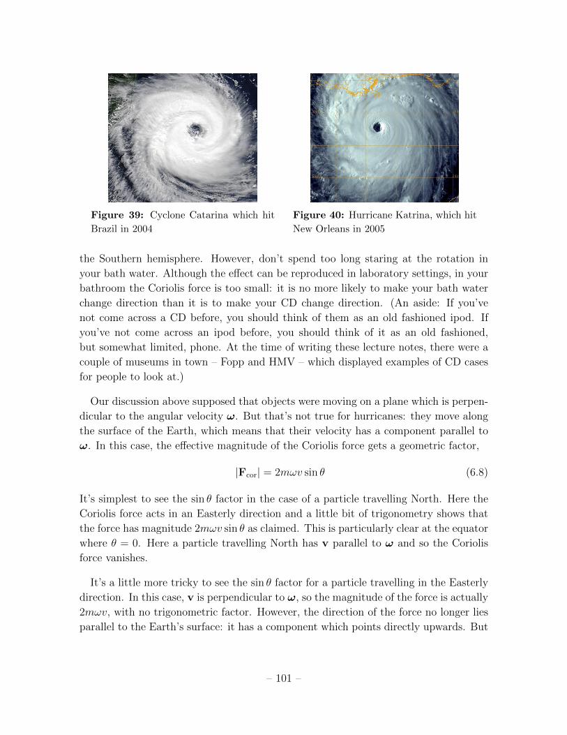
Figure 39: Cyclone Catarina which hit
Brazil in 2004
Figure 40: Hurricane Katrina, which hit
New Orleans in 2005
the Southern hemisphere. However, don’t spend too long staring at the rotation in
your bath water. Although the effect can be reproduced in laboratory settings, in your
bathroom the Coriolis force is too small: it is no more likely to make your bath water
change direction than it is to make your CD change direction. (An aside: If you’ve
not come across a CD before, you should think of them as an old fashioned ipod. If
you’ve not come across an ipod before, you should think of it as an old fashioned,
but somewhat limited, phone. At the time of writing these lecture notes, there were a
couple of museums in town – Fopp and HMV – which displayed examples of CD cases
for people to look at.)
Our discussion above supposed that objects were moving on a plane which is perpen-
dicular to the angular velocity ω. But that’s not true for hurricanes: they move along
the surface of the Earth, which means that their velocity has a component parallel to
ω. In this case, the effective magnitude of the Coriolis force gets a geometric factor,
|Fcor| = 2mωv sin θ (6.8)
It’s simplest to see the sin θ factor in the case of a particle travelling North. Here the
Coriolis force acts in an Easterly direction and a little bit of trigonometry shows that
the force has magnitude 2mωv sin θ as claimed. This is particularly clear at the equator
where θ = 0. Here a particle travelling North has v parallel to ω and so the Coriolis
force vanishes.
It’s a little more tricky to see the sin θ factor for a particle travelling in the Easterly
direction. In this case, v is perpendicular to ω, so the magnitude of the force is actually
2mωv, with no trigonometric factor. However, the direction of the force no longer lies
parallel to the Earth’s surface: it has a component which points directly upwards. But
– 101 –
we’re not interested in this component; it’s certainly not going to be big enough to
compete with gravity. Projecting onto the component that lies parallel to the Earth’s
surface (in a Southerly direction in this case), we again get a sin θ factor.
The factor of sin θ in (6.8) has an important meteorological consequence: the Coriolis
force vanishes when θ = 0, which ensures that hurricanes do not form within 500 miles
of the equator.
6.4.2 Balls and Towers
Climb up a tower and drop a ball. Where does it land? Since the Earth is rotating
under the tower, you might think that the ball lands behind you. In fact, it lands in
front! Let’s see where this somewhat counterintuitive result comes from.
The equation of motion in a rotating frame is
r = g − ω × (ω × r)− 2ω × r
We’ve already seen in Section 6.3.1 that the effect of the centrifugal force is to change
the effective direction of gravity. But we’ve also seen that this effect is small. In what
follows we will neglect the centrifugal term. In fact, we will ignore all terms of order
O(ω2) (there will be one more coming shortly!). We will therefore solve the equation
of motion
r = g − 2ω × r (6.9)
The first step is easy: we can integrate this once to give
r = gt− 2ω × (r− r0)
where we’ve introduced the initial position r0 as an integration constant. If we now
substitute this back into the equation of motion (6.9), we get a messy, but manageable,
equation. Let’s, however, make our life easier by recalling that we’ve already agreed to
drop terms of order O(ω2). Then, upon substitution, we’re left with
r ≈ g − 2ω × g t
which we can easily integrate one last time to find
r ≈ r0 +1
2gt2 − 1
3ω × g t3
– 102 –
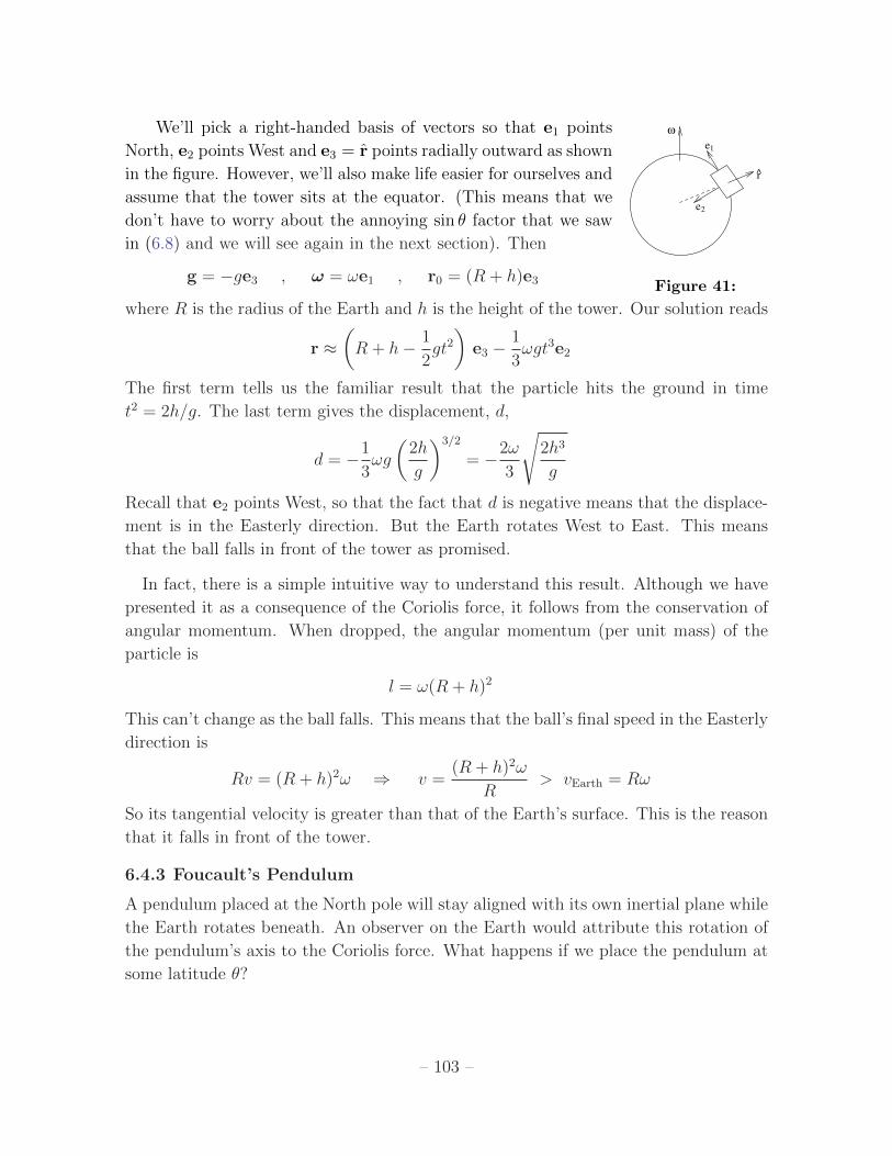
We’ll pick a right-handed basis of vectors so that e1 points
e2
ω
^
e1
r
Figure 41:
North, e2 points West and e3 = r points radially outward as shown
in the figure. However, we’ll also make life easier for ourselves and
assume that the tower sits at the equator. (This means that we
don’t have to worry about the annoying sin θ factor that we saw
in (6.8) and we will see again in the next section). Then
g = −ge3 , ω = ωe1 , r0 = (R + h)e3
where R is the radius of the Earth and h is the height of the tower. Our solution reads
r ≈(R + h− 1
2gt2)
e3 −1
3ωgt3e2
The first term tells us the familiar result that the particle hits the ground in time
t2 = 2h/g. The last term gives the displacement, d,
d = −1
3ωg
(2h
g
)3/2
= −2ω
3
√2h3
g
Recall that e2 points West, so that the fact that d is negative means that the displace-
ment is in the Easterly direction. But the Earth rotates West to East. This means
that the ball falls in front of the tower as promised.
In fact, there is a simple intuitive way to understand this result. Although we have
presented it as a consequence of the Coriolis force, it follows from the conservation of
angular momentum. When dropped, the angular momentum (per unit mass) of the
particle is
l = ω(R + h)2
This can’t change as the ball falls. This means that the ball’s final speed in the Easterly
direction is
Rv = (R + h)2ω ⇒ v =(R + h)2ω
R> vEarth = Rω
So its tangential velocity is greater than that of the Earth’s surface. This is the reason
that it falls in front of the tower.
6.4.3 Foucault’s Pendulum
A pendulum placed at the North pole will stay aligned with its own inertial plane while
the Earth rotates beneath. An observer on the Earth would attribute this rotation of
the pendulum’s axis to the Coriolis force. What happens if we place the pendulum at
some latitude θ?
– 103 –
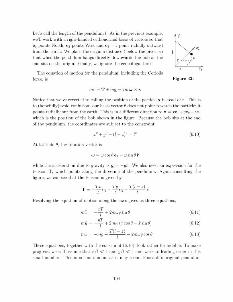
Let’s call the length of the pendulum l. As in the previous example,
e2
e1
r
x
yz
l
Figure 42:
we’ll work with a right-handed orthonormal basis of vectors so that
e1 points North, e2 points West and e3 = r point radially outward
from the earth. We place the origin a distance l below the pivot, so
that when the pendulum hangs directly downwards the bob at the
end sits on the origin. Finally, we ignore the centrifugal force.
The equation of motion for the pendulum, including the Coriolis
force, is
mr = T +mg − 2mω × x
Notice that we’ve reverted to calling the position of the particle x instead of r. This is
to (hopefully)avoid confusion: our basis vector r does not point towards the particle; it
points radially out from the earth. This is in a different direction to x = xe1 +ye2 +ze3
which is the position of the bob shown in the figure. Because the bob sits at the end
of the pendulum, the coordinates are subject to the constraint
x2 + y2 + (l − z)2 = l2 (6.10)
At latitude θ, the rotation vector is
ω = ω cos θ e1 + ω sin θ r
while the acceleration due to gravity is g = −gr. We also need an expression for the
tension T, which points along the direction of the pendulum. Again consulting the
figure, we can see that the tension is given by
T = −Txl
e1 −Ty
le2 +
T (l − z)
lr
Resolving the equation of motion along the axes gives us three equations,
mx = −xTl
+ 2mωy sin θ (6.11)
my = −yTl
+ 2mω (z cos θ − x sin θ) (6.12)
mz = −mg +T (l − z)
l− 2mωy cos θ (6.13)
These equations, together with the constraint (6.10), look rather formidable. To make
progress, we will assume that x/l 1 and y/l 1 and work to leading order in this
small number. This is not as random as it may seem: Foucault’s original pendulum
– 104 –
hangs in the Pantheon in Paris and is 67 meters long, with the amplitude of the swing
a few meters. The advantage of this approximation becomes apparent when we revisit
the constraint (6.10) which tells us that z/l is second order,
l − z = l
√1− x2
l2− y2
l2≈ l − x2
2l− y2
2l+ . . .
This means that, to leading order, we can set z, z and z all to zero. The last of the
equations (6.13) then provides an equation that will soon allow us to eliminate T
T ≈ mg + 2mωy cos θ (6.14)
Meanwhile, we rewrite the first two equations (6.11) and (6.12) using the same trick
we saw in our study of Larmor circles in Section (2.4.2): we introduce ξ = x + iy and
add (6.11) to i times (6.12) to get
ξ ≈ −glξ − 2ωiξ sin θ
Here we have substituted T ≈ mg since the second term in (6.14) contributes only at
sub-leading order. This is the equation of motion for a damped harmonic oscillator,
albeit with a complex variable. We can solve it in the same way: the ansatz ξ = eβt
results in the quadratic equation
β2 + 2iωβ sin θ +g
l= 0
which has solutions
β± = −iω sin θ ± i√
1
4ω2 sin2 θ +
g
l≈ −i
(ω sin θ ±
√g
l
)From this we can write the general solution as
ξ = e−iωt sin θ
(A cos
√g
lt+B sin
√g
lt
)Without the overall phase factor, e−iωt sin θ, this equation describes an ellipse. The
role of the phase factor is to make the orientation of the ellipse slowly rotate in the
x− y plane. Viewed from above, the rotation is clockwise in the Northern hemisphere;
anti-clockwise in the Southern hemisphere. Notice that the period of rotation is not 24
hours unless the pendulum is suspended at the poles. Instead the period is 24/ sin θ
hours. In Paris, this is 32 hours.
– 105 –

6.4.4 Larmor Precession
The transformation to rotating frames can also be used as a cute trick to solve certain
problems. Consider, for example, a charged particle orbiting around a second, fixed
particle under the influence of the Coulomb force. Now add to this a constant magnetic
field B. The resulting equation of motion is
mr = − kr2
r + qr×B
where k = qQ/4πε0. When B = 0, this is the central force problem that we solved in
Section 4 and we know the orbit of the particle is an ellipse. But what about when
B 6= 0?
Let’s look at the problem in a rotating frame. Using (6.3) and (6.4), we have
m (r + 2ω × r + ω × (ω × r)) = − kr2
r + q (r + ω × r)×B
where now r describes the position of the coordinate in the rotating frame. Now we do
something clever: we pick the angular velocity of rotation ω so that the r terms above
cancel. This works for
ω = − qB2m
Then the equation of motion becomes
mr = − kr2
r +q2
2mB× (B× r)
This is almost of the form that we studied in Section 4. In fact, for suitably small
magnetic fields we can just ignore the last term. This holds as long as B2 2mk/q2r3.
In this limit, we can just adopt our old solution of elliptic motion. However, transform-
ing back to the original frame, the ellipse will appear to rotate — or precess — with
angular speed
ω =qB
2m
This is known as the Larmor frequency. It is half of the cyclotron frequency that we
met in 2.4.2.
– 106 –

7. Special Relativity
Although Newtonian mechanics gives an excellent description of Nature, it is not uni-
versally valid. When we reach extreme conditions — the very small, the very heavy or
the very fast — the Newtonian Universe that we’re used to needs replacing. You could
say that Newtonian mechanics encapsulates our common sense view of the world. One
of the major themes of twentieth century physics is that when you look away from our
everyday world, common sense is not much use.
One such extreme is when particles travel very fast. The theory that replaces New-
tonian mechanics is due to Einstein. It is called special relativity. The effects of special
relativity become apparent only when the speeds of particles become comparable to
the speed of light in the vacuum. The speed of light is
c = 299792458 ms−1
This value of c is exact. It may seem strange that the speed of light is an integer
when measured in meters per second. The reason is simply that this is taken to be
the definition of what we mean by a meter: it is the distance travelled by light in
1/299792458 seconds. For the purposes of this course, we’ll be quite happy with the
approximation c ≈ 3× 10⁸ ms−1.
The first thing to say is that the speed of light is fast. Really fast. The speed of
sound is around 300 ms−1; escape velocity from the Earth is around 104 ms−1; the
orbital speed of our solar system in the Milky Way galaxy is around 105 ms−1. As we
shall soon see, nothing travels faster than c.
The theory of special relativity rests on two experimental facts. (We will look at the
evidence for these shortly). In fact, we have already met the first of these: it is simply
the Galilean principle of relativity described in Section 1. The second postulate is more
surprising:
• Postulate 1: The principle of relativity: the laws of physics are the same in all
inertial frames
• Postulate 2: The speed of light in vacuum is the same in all inertial frames
On the face of it, the second postulate looks nonsensical. How can the speed of light
look the same in all inertial frames? If light travels towards me at speed c and I run
away from the light at speed v, surely I measure the speed of light as c − v. Right?
Well, no.
– 107 –

This common sense view is encapsulated in the Galilean transformations that we
met in Section 1.2.1. Mathematically, we derive this “obvious” result as follows: two
inertial frames, S and S ′, which move relative to each with velocity v = (v, 0, 0), have
Cartesian coordinates related by
x′ = x− vt , y′ = y , z′ = z , t′ = t (7.1)
If a ray of light travels in the x direction in frame S with speed c, then it traces out
the trajectory x/t = c. The transformations above then tell us that in frame S ′ the
trajectory if the light ray is x′/t′ = c − v. This is the result we claimed above: the
speed of light should clearly be c − v. If this is wrong (and it is) something must be
wrong with the Galilean transformations (7.1). But what?
Our immediate goal is to find a transformation law that obeys both postulates above.
As we will see, the only way to achieve this goal is to allow for a radical departure in
our understanding of time. In particular, we will be forced to abandon the assumption
of absolute time, enshrined in the equation t′ = t above. We will see that time ticks at
different rates for observers sitting in different inertial frames.
7.1 Lorentz Transformations
We stick with the idea of two inertial frames, S and S ′, moving with relative speed v.
For simplicity, we’ll start by ignoring the directions y and z which are perpendicular to
the direction of motion. Both inertial frames come with Cartesian coordinates: (x, t)
for S and (x′, t′) for S ′. We want to know how these are related. The most general
possible relationship takes the form
x′ = f(x, t) , t′ = g(x, t)
for some function f and g. However, there are a couple of facts that we can use to
immediately restrict the form of these functions. The first is that the law of inertia
holds; left alone in an inertial frame, a particle will travel at constant velocity. Drawn
in the (x, t) plane, the trajectory of such a particle is a straight line. Since both S and
S ′ are inertial frames, the map (x, t) 7→ (x′, t′) must map straight lines to straight lines;
such maps are, by definition, linear. The functions f and g must therefore be of the
form
x′ = α1x+ α2t , t′ = α3x+ α4t
where αi, i = 1, 2, 3, 4 can each be a function of v.
– 108 –
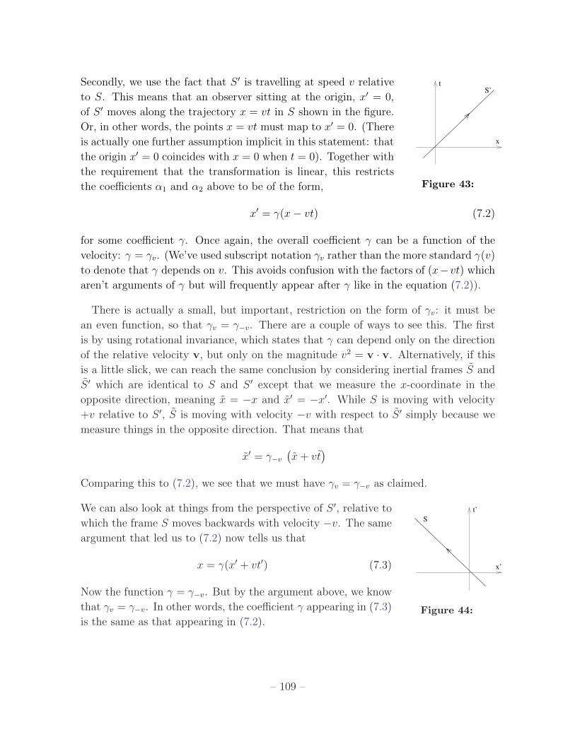
Secondly, we use the fact that S ′ is travelling at speed v relative t
x
S’
Figure 43:
to S. This means that an observer sitting at the origin, x′ = 0,
of S ′ moves along the trajectory x = vt in S shown in the figure.
Or, in other words, the points x = vt must map to x′ = 0. (There
is actually one further assumption implicit in this statement: that
the origin x′ = 0 coincides with x = 0 when t = 0). Together with
the requirement that the transformation is linear, this restricts
the coefficients α1 and α2 above to be of the form,
x′ = γ(x− vt) (7.2)
for some coefficient γ. Once again, the overall coefficient γ can be a function of the
velocity: γ = γv. (We’ve used subscript notation γv rather than the more standard γ(v)
to denote that γ depends on v. This avoids confusion with the factors of (x−vt) which
aren’t arguments of γ but will frequently appear after γ like in the equation (7.2)).
There is actually a small, but important, restriction on the form of γv: it must be
an even function, so that γv = γ−v. There are a couple of ways to see this. The first
is by using rotational invariance, which states that γ can depend only on the direction
of the relative velocity v, but only on the magnitude v2 = v · v. Alternatively, if this
is a little slick, we can reach the same conclusion by considering inertial frames S and
S ′ which are identical to S and S ′ except that we measure the x-coordinate in the
opposite direction, meaning x = −x and x′ = −x′. While S is moving with velocity
+v relative to S ′, S is moving with velocity −v with respect to S ′ simply because we
measure things in the opposite direction. That means that
x′ = γ−v(x+ vt
)Comparing this to (7.2), we see that we must have γv = γ−v as claimed.
We can also look at things from the perspective of S ′, relative to t’
x’
S
Figure 44:
which the frame S moves backwards with velocity −v. The same
argument that led us to (7.2) now tells us that
x = γ(x′ + vt′) (7.3)
Now the function γ = γ−v. But by the argument above, we know
that γv = γ−v. In other words, the coefficient γ appearing in (7.3)
is the same as that appearing in (7.2).
– 109 –

At this point, things don’t look too different from what we’ve seen before. Indeed, if
we now insisted on absolute time, so t = t′, we’re forced to have γ = 1 and we get back
to the Galilean transformations (7.1). However, as we’ve seen, this is not compatible
with the second postulate of special relativity. So let’s push forward and insist instead
that the speed of light is equal to c in both S and S ′. In S, a light ray has trajectory
x = ct
While, in S ′, we demand that the same light ray has trajectory
x′ = ct′
Substituting these trajectories into (7.2) and (7.3), we have two equations relating t
and t′,
ct′ = γ(c− v)t and ct = γ(c+ v)t′
A little algebra shows that these two equations are compatible only if γ is given by
γ =
√1
1− v2/c2(7.4)
We’ll be seeing a lot of this coefficient γ in what follows. Notice that for v c, we
have γ ≈ 1 and the transformation law (7.2) is approximately the same as the Galilean
transformation (7.1). However, as v → c we have γ → ∞. Furthermore, γ becomes
imaginary for v > c which means that we’re unable to make sense of inertial frames
with relative speed v > c.
Equations (7.2) and (7.4) give us the transformation law for the spatial coordinate.
But what about for time? In fact, the temporal transformation law is already lurking in
our analysis above. Substituting the expression for x′ in (7.2) into (7.3) and rearranging,
we get
t′ = γ(t− v
c2x)
(7.5)
We shall soon see that this equation has dramatic consequences. For now, however, we
merely note that when v c, we recover the trivial Galilean transformation law t′ ≈ t.
Equations (7.2) and (7.5) are the Lorentz transformations.
– 110 –
7.1.1 Lorentz Transformations in Three Spatial Dimensions
In the above derivation, we ignored the transformation of the coordinates y and z
perpendicular to the relative motion. In fact, these transformations are trivial. Using
the above arguments for linearity and the fact that the origins coincide at t = 0, the
most general form of the transformation is
y′ = κy
But, by symmetry, we must also have y = κy′. Clearly, we require κ = 1. (The other
possibility κ = −1 does not give the identity transformation when v = 0. Instead, it is
a reflection).
With this we can write down the final form of the Lorentz transformations. Note
that they look more symmetric between x and t if we write them using the combination
ct,
x′ = γ(x− v
cct)
y′ = y
z′ = z (7.6)
ct′ = γ(ct− v
cx)
where γ is given by (7.4). These are also known as Lorentz boosts. Notice that for
v/c 1, the Lorentz boosts reduce to the more intuitive Galilean boosts that we saw
in Section 1. (We sometimes say, rather sloppily, that the Lorentz transformations
reduce to the Galilean transformations in the limit c→∞).
It’s also worth stressing again the special properties of these transformations. To be
compatible with the first postulate, the transformations must take the same form if we
invert them to express x and t in terms of x′ and t′, except with v replaced by −v.
And, after a little bit of algebraic magic, they do.
Secondly, we want the speed of light to be the same in all inertial frames. For light
travelling in the x direction, we already imposed this in our derivation of the Lorentz
transformations. But it’s simple to check again: in frame S, the trajectory of an object
travelling at the speed of light obeys x = ct. In S ′, the same object will follow the
trajectory x′ = γ(x− vt) = γ(ct− vx/c) = ct′.
– 111 –

ct
x
P
ct
x
Figure 45: The worldline of a particle Figure 46: Light rays travel at 45
What about an object travelling in the y direction at the speed of light? Its trajectory
in S is y = ct. From (7.6), its trajectory in S ′ is y′ = ct′/γ and x′ = −vt′. Its speed in
S ′ is therefore v′ 2 = v2x + v2
y, or
v′ 2 =
(x′
t′
)2
+
(y′
t′
)2
= v2 +c2
γ2= c2
7.1.2 Spacetime Diagrams
We’ll find it very useful to introduce a simple spacetime diagram to illustrate the physics
of relativity. In a fixed inertial frame, S, we draw one direction of space — say x —
along the horizontal axis and time on the vertical axis. But things look much nicer if
we rescale time and plot ct on the vertical instead. In the context of special relativity,
space and time is called Minkowski space. (Although the true definition of Minkowski
space requires some extra structure on space and time which we will meet in Section
(7.3)).
This is a spacetime diagram. Each point, P , represents an event. In the following,
we’ll label points on the spacetime diagram as coordinates (ct, x) i.e. giving the coor-
dinate along the vertical axis first. This is backwards from the usual way coordinates
but is chosen so that it is consistent with a later, standard, convention that we will
meet in Section 7.3.
A particle moving in spacetime traces out a curve called a worldline as shown in
the figure. Because we’ve rescaled the time axis, a light ray moving in the x direction
moves at 45. We’ll later see that no object can move faster than the speed of light
which means that the worldlines of particles must always move upwards at an angle
steeper than 45.
– 112 –

The horizontal and vertical axis in the spacetime diagram are the coordinates of the
inertial frame S. But we could also draw the axes corresponding to an inertial frame
S ′ moving with relative velocity v = (v, 0, 0). The t′ axis sits at x′ = 0 and is given by
x = vt
Meanwhile, the x′ axis is determined by t′ = 0 which, fromct
x
x’
ct’
Figure 47:
the Lorentz transformation (7.6), is given by the equation
ct =v
cx
These two axes are drawn on the figure to the right. They
can be the thought of as the x and ct axes, rotated by an
equal amount towards the diagonal light ray. The fact
the axes are symmetric about the light ray reflects the
fact that the speed of light is equal to c in both frames.
7.1.3 A History of Light Speed
The first evidence that light does not travel instantaneously was presented by the
Danish Astronomer Ole Rømer in 1676. He noticed that the periods of the orbits of Io,
the innermost moon of Jupiter, are not constant. When the Earth is moving towards
Jupiter, the orbits are a few minutes shorter; when the Earth moves away, the orbits
are longer by the same amount. Rømer correctly deduced that this was due to the
finite speed of light and gave a rough estimate for the value of c.
By the mid 1800s, the speed of light had been determined fairly accurately using
experiments involving rotating mirrors. Then came a theoretical bombshell. Maxwell
showed that light could be understood as oscillations of the electric and magnetic
fields. He related the speed of light to two constants, ε0 and µ0, the permittivity and
permeability of free space, that arise in the theory of electromagnetism,
c =
√1
ε0µ0
(7.7)
But, as we have seen, Newtonian physics tells us that speeds are relative. If Maxwell’s
equations predict a value for the speed of light, it was thought that these equations must
be valid only in a preferred reference frame. Moreover, this does not seem unreasonable;
if light is a wave then surely there is something waving. Just as water waves need
water, and sound waves need air, so it was thought that light waves need a material
to propagate in. This material was dubbed the luminiferous ether and it was thought
that Maxwell’s equations must only be valid in the frame at rest with respect to this
ether.
– 113 –

In 1881, Michelson and Morley performed an experiment to detect the relative motion
of the Earth through the ether. Since the Earth is orbiting the Sun at a speed of
3 × 10⁴ ms−1, even if it happens to be stationary with respect to the ether at some
point, six months later this can no longer be the case.
Suppose that at some moment the Earth is moving in the x-direction relative to
the ether with some speed v. The Newtonian addition of velocities tells us that light
propagating in the x-direction should have speed c+ v going one way and c− v going
the other. The total time to travel backwards and forwards along a length L should
therefore be
Tx =L
c+ v+
L
c− v=
2cL
c2 − v2
Meanwhile, light making the same journey in the y-direction will have to travel (by
Pythagoras) a total distance of√L2 + v2(Ty/2)2 on each leg of the journey. It makes
this journey at speed c, meaning that we can equate
cTy2
=√L2 + v2(Ty/2)2 ⇒ Ty =
2L√c2 − v2
The goal of the Michelson-Morley experiment was to measure the time difference be-
tween Ty and Tx using interference patterns of light ray making the two journeys.
Needless to say, the experiment didn’t work: there seemed to be no difference in the
time taken to travel in the x direction and y direction.
Towards the end of the 1800s, the null result of the Michelson-Morley experiment
had become one of the major problems in theoretical physics. Several explanations
were proposed, including the idea that the ether was somehow dragged along with the
Earth. The Dutch physicist, Hendrik Lorentz, went some way to finding the correct
solution. He had noticed that Maxwell’s equations had the peculiar symmetry that we
now call the Lorentz transformations. He argued that if a reason could be found that
would allow distances between matter to change as
x′ = γ(x− vt)
then lengths would be squeezed in the direction parallel to the ether, explaining why
no difference is seen between Tx and Ty. (We will shortly derive this contraction of
lengths using special relativity). Lorentz set to work trying to provide a mechanical
explanation for this transformation law.
– 114 –
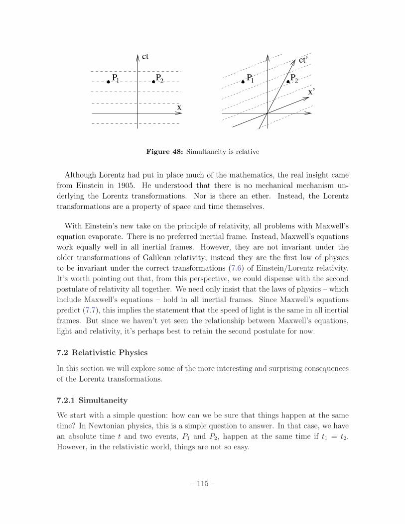
P1
P2
P1
P2
ct
x
ct’
x’
Figure 48: Simultaneity is relative
Although Lorentz had put in place much of the mathematics, the real insight came
from Einstein in 1905. He understood that there is no mechanical mechanism un-
derlying the Lorentz transformations. Nor is there an ether. Instead, the Lorentz
transformations are a property of space and time themselves.
With Einstein’s new take on the principle of relativity, all problems with Maxwell’s
equation evaporate. There is no preferred inertial frame. Instead, Maxwell’s equations
work equally well in all inertial frames. However, they are not invariant under the
older transformations of Galilean relativity; instead they are the first law of physics
to be invariant under the correct transformations (7.6) of Einstein/Lorentz relativity.
It’s worth pointing out that, from this perspective, we could dispense with the second
postulate of relativity all together. We need only insist that the laws of physics – which
include Maxwell’s equations – hold in all inertial frames. Since Maxwell’s equations
predict (7.7), this implies the statement that the speed of light is the same in all inertial
frames. But since we haven’t yet seen the relationship between Maxwell’s equations,
light and relativity, it’s perhaps best to retain the second postulate for now.
7.2 Relativistic Physics
In this section we will explore some of the more interesting and surprising consequences
of the Lorentz transformations.
7.2.1 Simultaneity
We start with a simple question: how can we be sure that things happen at the same
time? In Newtonian physics, this is a simple question to answer. In that case, we have
an absolute time t and two events, P1 and P2, happen at the same time if t1 = t2.
However, in the relativistic world, things are not so easy.
– 115 –

We start with an observer in inertial frame S, with time coordinate t. This observer
sensibly decides that two events, P1 and P2, occur simultaneously if t1 = t2. In the
spacetime diagram on the left of Figure 48 we have drawn lines of simultaneity for this
observer.
But for an observer in the inertial frame S ′, simultaneity of events occurs for equal
t′. Using the Lorentz transformation, lines of constant t′ become lines described by the
equation t− vx/c2 = constant. These lines are drawn on the spacetime diagram on the
right of Figure 48.
The upshot of this is that two events simultaneous in one inertial frame are not
simultaneous in another. An observer in S thinks that events P1 and P2 happen at the
same time. All other observers disagree.
A Train Story
v
Figure 49: Lights on Trains: Simultaneity is Relative
The fact that all observers cannot agree on what events are simultaneous is a
direct consequence of the fact that all observers do agree on the speed of light. We
can illustrate this connection with a simple gedankenexperiment. (An ugly German
word for “thought experiment”, a favourite trick of theoretical physicists who can’t be
bothered to do real experiments). Consider a train moving at constant speed, with a
lightbulb hanging from the middle of one of the carriages. A passenger on the train
turns on the bulb and, because the bulb is equidistant from both the front and back
wall of the carriage, observes that the light hits both walls at the same time.
However, a person standing on the platform as the train passes through disagrees.
The light from the bulb travels at equal speed ±c to the left and right, but the back of
the train is rushing towards the point in space where the light first emerged from. The
person on the platform will see the light hit the back of the train first.
– 116 –
It is worth mentioning that although the two people disagree on whether the light
hits the walls at the same time, this does not mean that they can’t be friends.
A Potential Confusion: What the Observer Observes
We’ll pause briefly to press home a point that may lead to confusion. You might
think that the question of simultaneity has something to do with the finite speed of
propagation. You don’t see something until the light has travelled to you, just as you
don’t hear something until the sound has travelled to you. This is not what’s going on
here! A look at the spacetime diagram in Figure 48 shows that we’ve already taken
this into account when deciding whether two events occur simultaneously. The lack of
simultaneity between moving observers is a much deeper issue, not due to the finiteness
of the speed of light but rather due to the constancy of the speed of light.
The confusion about the time of flight of the signal is sometimes compounded by
the common use of the word observer to mean “inertial frame”. This brings to mind
some guy sitting at the origin, surveying all around him. Instead, you should think of
the observer more as a Big Brother figure: a sea of clocks and rulers throughout the
inertial frame which can faithfully record and store the position and time of any event,
to be studied at some time in the future.
Of course, this means that there is a second question we can ask which is: what
does the guy sitting at the origin actually see? Now we have to take into account
both the relative nature of simultaneity and the issues related with the finite speed of
propagation. This adds an extra layer of complexity which we will discuss in Section
7.6.
7.2.2 Causality
We’ve seen that different observers disagree on the temporal ordering of two events.
But where does that leave the idea of causality? Surely it’s important that we can say
that one event definitely occurred before another. Thankfully, all is not lost: there are
only some events which observers can disagree about.
To see this, note that because Lorentz boosts are only possible for v < c, the lines of
simultaneity cannot be steeper than 45. Take a point P and draw the 45 light rays
that emerge from P . This is called the light cone. (For once, in the figure, I’ve drawn
this with an extra spatial dimension present to illustrate how this works in spatial
dimensions bigger than one). The light cone is really two cones, touching at the point
P . They are known as the future light cone and past light cone.
– 117 –

For events inside the light cone of P , there is no dif-
x
ct
R
P
Q
Figure 50:
ficulty deciding on the temporal ordering of events. All ob-
servers will agree that Q occurred after P . However, for events
outside the light cone, the matter is up for grabs: some ob-
servers will see R as happening after P ; some before.
This tells us that the events which all observers agree can
be causally influenced by P are those inside the future light
cone. Similarly, the events which can plausibly influence P
are those inside the past light cone. This means that we can
sleep comfortably at night, happy in the knowledge that causality is preserved, only if
nothing can propagate outside the light cone. But that’s the same thing as travelling
faster than the speed of light.
The converse to this is that if we do ever see particles that travel faster than the
speed of light, we’re in trouble. We could use them to transmit information faster than
light. But another observer would view this as transmitting information backwards in
time. All our ideas of cause and effect will be turned on their head. You will therefore
be relieved to learn that we will show in Section 7.3 why it is impossible to accelerate
particles past the light speed barrier.
There is a corollary to the statement that events outside the lightcone cannot influ-
ence each other: there are no perfectly rigid objects. Suppose that you push on one
end of a rod. The other end cannot move immediately since that would allow us to
communicate faster than the speed of light. Of course, for real rods, the other end does
not move instantaneously. Instead, pushing on one end of the rod initiates a sound
wave which propagates through the rod, telling the other parts to move. The state-
ment that there is no rigid object is simply the statement that this sound wave must
travel slower than the speed of light.
Finally, let me mention that when we’re talking about waves, as opposed to point
particles, there is a slight subtlety in exactly what must travel slower than light. There
are at least two velocities associated to a wave: the group velocity is (usually) the speed
at which information can be communicated. This is less than c. In contrast, the phase
velocity is the speed at which the peaks of the wave travel. This can be greater than
c, but transmits no information.
7.2.3 Time Dilation
We’ll now turn to one of the more dramatic results of special relativity. Consider a
clock sitting stationary in the frame S ′ which ticks at intervals of T ′. This means that
– 118 –
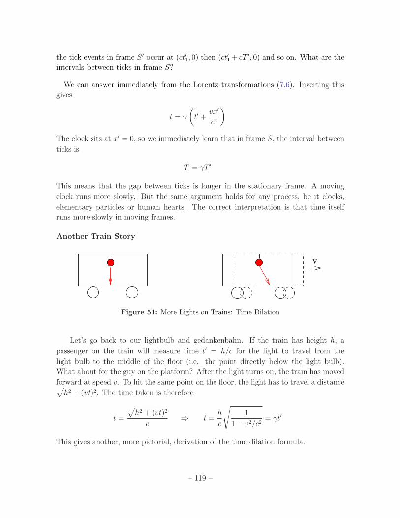
the tick events in frame S ′ occur at (ct′1, 0) then (ct′1 + cT ′, 0) and so on. What are the
intervals between ticks in frame S?
We can answer immediately from the Lorentz transformations (7.6). Inverting this
gives
t = γ
(t′ +
vx′
c2
)The clock sits at x′ = 0, so we immediately learn that in frame S, the interval between
ticks is
T = γT ′
This means that the gap between ticks is longer in the stationary frame. A moving
clock runs more slowly. But the same argument holds for any process, be it clocks,
elementary particles or human hearts. The correct interpretation is that time itself
runs more slowly in moving frames.
Another Train Story
v
Figure 51: More Lights on Trains: Time Dilation
Let’s go back to our lightbulb and gedankenbahn. If the train has height h, a
passenger on the train will measure time t′ = h/c for the light to travel from the
light bulb to the middle of the floor (i.e. the point directly below the light bulb).
What about for the guy on the platform? After the light turns on, the train has moved
forward at speed v. To hit the same point on the floor, the light has to travel a distance√h2 + (vt)2. The time taken is therefore
t =
√h2 + (vt)2
c⇒ t =
h
c
√1
1− v2/c2= γt′
This gives another, more pictorial, derivation of the time dilation formula.
– 119 –

On Muons and Planes
Away from the world of gedankenexperiments, there are a couple of real experimental
consequences of time dilation. Certainly the place that this phenomenon is tested most
accurately is in particle accelerators where elementary particles routinely reach speeds
close to c. The protons spinning around the LHC have γ ≈ 3500. The previous collider
in CERN, called LEP, accelerated electrons and positrons to γ ≈ 2 × 10⁵. (Although
the electrons in LEP were travelling faster than the protons in LHC, the greater mass
of the protons means that there is substantially more energy in the LHC collisions).
The effect of time dilation is particularly vivid on unstable particles which live much
longer in the lab frame than in their own rest frame. An early demonstration was seen
in muons in 1941. These are heavier, unstable, versions of the electron. They decay
into an electron, together with a couple of neutrinos, with a half-life of τ ≈ 2× 10⁻⁶ s.
Muons are created when cosmic rays hit the atmosphere, and subsequently rain down
on Earth. Yet to make it down to sea level, it takes about t = 7 × 10⁻⁶ s, somewhat
longer than their lifetime. Given this, why are there any muons detected on Earth
at all? Surely they should have decayed. The reason that they do not is because the
muons are travelling at a speed v ≈ 0.99c, giving γ ≈ 10. From the muon’s perspective,
the journey only takes t′ = t/γ ≈ 7× 10⁻⁷ s, somewhat less than their lifetime.
Note that elementary particles are, by definition, structureless. They’re certainly
not some clock with an internal machinery. The reason that they live longer can’t be
explained because of some mechanical device which slows down: it is time itself which
is running slower.
A more direct test of time dilation was performed in 1971 by Hafele and Keating.
They flew two atomic clocks around the world on commercial airliners; two more were
left at home. When they were subsequently brought together, their times differed by
about 10−7 s. There are actually two contributions to this effect: the time dilation
of special relativity that we’ve seen above, together with a related effect in general
relativity due to the gravity of the Earth.
Twin Paradox
Two twins, Luke and Leia, decide to spend some time apart. Leia stays at home while
Luke jumps in a spaceship and heads at some speed v to the planet Tatooine. With
sadness, Leia watches Luke leave but is relieved to see — only a time T later from her
perspective — him safely reach the planet.
– 120 –
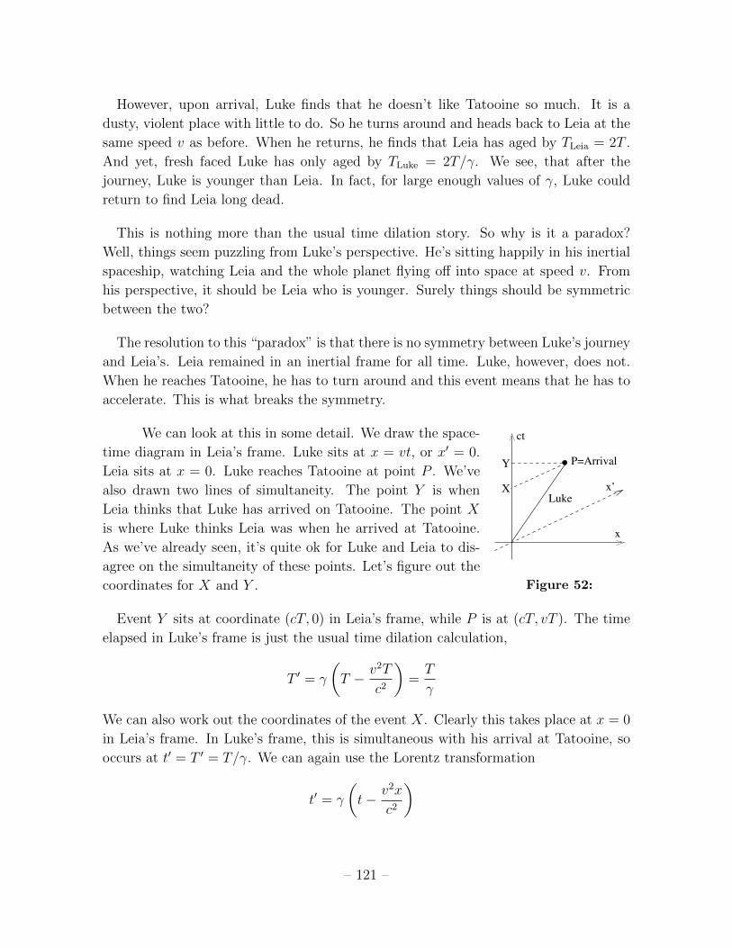
However, upon arrival, Luke finds that he doesn’t like Tatooine so much. It is a
dusty, violent place with little to do. So he turns around and heads back to Leia at the
same speed v as before. When he returns, he finds that Leia has aged by TLeia = 2T .
And yet, fresh faced Luke has only aged by TLuke = 2T/γ. We see, that after the
journey, Luke is younger than Leia. In fact, for large enough values of γ, Luke could
return to find Leia long dead.
This is nothing more than the usual time dilation story. So why is it a paradox?
Well, things seem puzzling from Luke’s perspective. He’s sitting happily in his inertial
spaceship, watching Leia and the whole planet flying off into space at speed v. From
his perspective, it should be Leia who is younger. Surely things should be symmetric
between the two?
The resolution to this “paradox” is that there is no symmetry between Luke’s journey
and Leia’s. Leia remained in an inertial frame for all time. Luke, however, does not.
When he reaches Tatooine, he has to turn around and this event means that he has to
accelerate. This is what breaks the symmetry.
We can look at this in some detail. We draw the space- ct
x’
x
X
Y
Luke
P=Arrival
Figure 52:
time diagram in Leia’s frame. Luke sits at x = vt, or x′ = 0.
Leia sits at x = 0. Luke reaches Tatooine at point P . We’ve
also drawn two lines of simultaneity. The point Y is when
Leia thinks that Luke has arrived on Tatooine. The point X
is where Luke thinks Leia was when he arrived at Tatooine.
As we’ve already seen, it’s quite ok for Luke and Leia to dis-
agree on the simultaneity of these points. Let’s figure out the
coordinates for X and Y .
Event Y sits at coordinate (cT, 0) in Leia’s frame, while P is at (cT, vT ). The time
elapsed in Luke’s frame is just the usual time dilation calculation,
T ′ = γ
(T − v2T
c2
)=T
γ
We can also work out the coordinates of the event X. Clearly this takes place at x = 0
in Leia’s frame. In Luke’s frame, this is simultaneous with his arrival at Tatooine, so
occurs at t′ = T ′ = T/γ. We can again use the Lorentz transformation
t′ = γ
(t− v2x
c2
)
– 121 –
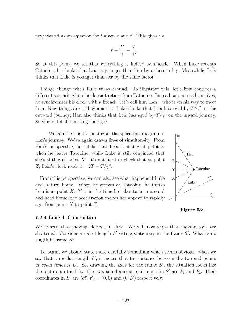
now viewed as an equation for t given x and t′. This gives us
t =T ′
γ=T
γ2
So at this point, we see that everything is indeed symmetric. When Luke reaches
Tatooine, he thinks that Leia is younger than him by a factor of γ. Meanwhile, Leia
thinks that Luke is younger than her by the same factor .
Things change when Luke turns around. To illustrate this, let’s first consider a
different scenario where he doesn’t return from Tatooine. Instead, as soon as he arrives,
he synchronises his clock with a friend – let’s call him Han – who is on his way to meet
Leia. Now things are still symmetric. Luke thinks that Leia has aged by T/γ2 on the
outward journey; Han also thinks that Leia has aged by T/γ2 on the inward journey.
So where did the missing time go?
We can see this by looking at the spacetime diagram of
Tatooine
x’
x
X
Y
ct
Z
Luke
Han
Figure 53:
Han’s journey. We’ve again drawn lines of simultaneity. From
Han’s perspective, he thinks that Leia is sitting at point Z
when he leaves Tatooine, while Luke is still convinced that
she’s sitting at point X. It’s not hard to check that at point
Z, Leia’s clock reads t = 2T − T/γ2.
From this perspective, we can also see what happens if Luke
does return home. When he arrives at Tatooine, he thinks
Leia is at point X. Yet, in the time he takes to turn around
and head home, the acceleration makes her appear to rapidly
age, from point X to point Z.
7.2.4 Length Contraction
We’ve seen that moving clocks run slow. We will now show that moving rods are
shortened. Consider a rod of length L′ sitting stationary in the frame S ′. What is its
length in frame S?
To begin, we should state more carefully something which seems obvious: when we
say that a rod has length L′, it means that the distance between the two end points
at equal times is L′. So, drawing the axes for the frame S ′, the situation looks like
the picture on the left. The two, simultaneous, end points in S ′ are P1 and P2. Their
coordinates in S ′ are (ct′, x′) = (0, 0) and (0, L′) respectively.
– 122 –

P1 P
2 P1
P2
ct’
x’
x’
ct
x
L’L
Figure 54: Length Contraction
Now let’s look at this in frame S. This is drawn in right-hand picture. Clearly P1
sits at (ct, x) = (0, 0). Meanwhile, the Lorentz transformation gives us the coordinate
for P2
x = γL′ and t =γvL′
c2
But to measure the rod in frame S, we want both ends to be at the same time. And
the points P1 and P2 are not simultaneous in S. We can follow the point P2 backwards
along the trajectory of the end point to Q2, which sits at
x = γL′ − vt
We want Q2 to be simultaneous with P1 in frame S. This means we must move back
a time t = γvL/c2, giving
x = γL′ − γv2L′
c2=L′
γ
This is telling us that the length L measured in frame S is
L =L′
γ
It is shorter than the length of the rod in its rest frame by a factor of γ. This phe-
nomenon is known as Lorentz contraction.
Putting Ladders in Barns
Take a ladder of length 2L and try to put it in a barn of length L. If you run fast enough,
can you squeeze it? Here are two arguments, each giving the opposite conclusion
– 123 –
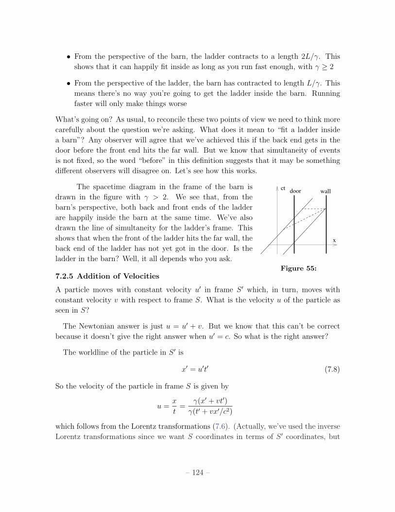
• From the perspective of the barn, the ladder contracts to a length 2L/γ. This
shows that it can happily fit inside as long as you run fast enough, with γ ≥ 2
• From the perspective of the ladder, the barn has contracted to length L/γ. This
means there’s no way you’re going to get the ladder inside the barn. Running
faster will only make things worse
What’s going on? As usual, to reconcile these two points of view we need to think more
carefully about the question we’re asking. What does it mean to “fit a ladder inside
a barn”? Any observer will agree that we’ve achieved this if the back end gets in the
door before the front end hits the far wall. But we know that simultaneity of events
is not fixed, so the word “before” in this definition suggests that it may be something
different observers will disagree on. Let’s see how this works.
The spacetime diagram in the frame of the barn is ct
x
door wall
Figure 55:
drawn in the figure with γ > 2. We see that, from the
barn’s perspective, both back and front ends of the ladder
are happily inside the barn at the same time. We’ve also
drawn the line of simultaneity for the ladder’s frame. This
shows that when the front of the ladder hits the far wall, the
back end of the ladder has not yet got in the door. Is the
ladder in the barn? Well, it all depends who you ask.
7.2.5 Addition of Velocities
A particle moves with constant velocity u′ in frame S ′ which, in turn, moves with
constant velocity v with respect to frame S. What is the velocity u of the particle as
seen in S?
The Newtonian answer is just u = u′ + v. But we know that this can’t be correct
because it doesn’t give the right answer when u′ = c. So what is the right answer?
The worldline of the particle in S ′ is
x′ = u′t′ (7.8)
So the velocity of the particle in frame S is given by
u =x
t=
γ(x′ + vt′)
γ(t′ + vx′/c2)
which follows from the Lorentz transformations (7.6). (Actually, we’ve used the inverse
Lorentz transformations since we want S coordinates in terms of S ′ coordinates, but
– 124 –

these differ only changing −v to v). Substituting (7.8) into the expression above, and
performing a little algebra, gives us the result we want:
u =u′ + v
1 + u′v/c2(7.9)
Note that when u′ = c, this gives us u = c as expected.
We can also show that if |u′| < c and |v| < c then we necessarily have −c < u < c.
The proof is simple algebra, if a little fiddly
c− u = c− u′ + v
1 + u′v/c2=c(c− u′)(c− v)
c2 + u′v> 0
where the last equality follows because, by our initial assumptions, each factor in the
final expression is positive. An identical calculation will show you that −c < u as well.
We learn that if a particle is travelling slower than the speed of light in one inertial
frame, it will also be travelling slower than light in all others.
7.3 The Geometry of Spacetime
The views of space and time which I wish to lay before you have sprung from
the soil of experimental physics, and therein lies their strength. They are
radical. Henceforth space by itself, and time by itself, are doomed to fade
away into mere shadows, and only a kind of union of the two will preserve
an independent reality.
Hermann Minkowski, 1908
We have seen that time is relative, length is relative, simultaneity is relative. Is
nothing sacred anymore? Well, the answer is yes: there is one measurement that all
observers will agree on.
7.3.1 The Invariant Interval
Let’s start by considering a spacetime with just a single spatial coordinate, x. In
frame S, two events P1 and P2 have coordinates (ct1, x1) and (ct2, x2). The events are
separated by ∆t = t1 − t2 in time and ∆x = x1 − x2 in space.
We define the invariant interval ∆s2 as a measure of the distance between these two
points:
∆s2 = c2∆t2 −∆x2
– 125 –

The advantage of the invariant interval is that it is something all observers agree upon.
In frame S ′, we have
∆s2 = γ2
(c∆t′ +
v∆x′
c
)2
− γ2 (∆x′ + v∆t′)2
= γ2(c2 − v2)∆t′ 2 − γ2
(1− v2
c2
)∆x′ 2 (7.10)
= c2∆t′ 2 −∆x′ 2
where, in going from the first line to the second, we see that the cross-terms ∆t′∆x′
cancel out.
Including all three spatial dimensions, the definition of the invariant interval is
∆s2 = c2∆t2 −∆x2 −∆y2 −∆z2 (7.11)
which, again, is the same in all frames. (The only non-trivial part of the calculation is
(7.10) above since y and z are invariant under a boost in the x direction).
The spacetime of special relativity is topologically R4. When endowed with the
measure of distance (7.11), this spacetime is referred to as Minkowski space. Although
topologically equivalent to Euclidean space, distances are measured differently. To
stress the difference between the time and spatial directions, Minkowski space is some-
times said to have dimension d = 1 + 3. (For once, it’s important that you don’t do
this sum!).
In later courses — in particular General Relativity — you will see the invariant
interval written as the distance between two infinitesimally close points. In practice
that just means we replace all the ∆(something)s with d(something)s.
ds2 = c2dt2 − dx2 − dy2 − dz2
In this infinitesimal form, ds2 is called the line element.
The invariant interval provides an observer-independent characterisation of the dis-
tance between any two events. However, it has a strange property: it is not positive
definite. Two events whose separation is ∆s2 > 0 are said to be timelike separated.
They are closer together in space than they are in time. Pictorially, such events sit
within each others light cone.
– 126 –

In contrast, events with ∆s2 < 0 are said to be spacelike separated. They sit outside
each others light cone. From our discussion in Section 7.2.2, we know that two observers
can disagree about the temporal ordering of spacelike separated events. However,
they agree on the ordering of timelike separated events. Note that since ∆s2 < 0 for
spacelike separated events, if you insist on talking about ∆s itself then it must be
purely imaginary. However, usually it will be perfectly fine if we just talk about ∆s2.
Finally, two events with ∆s2 = 0 are said to be lightlike separated. Notice that this
is an important difference between the invariant interval and most measures of distance
that you’re used to. Usually, if two points are separated by zero distance, then they are
the same point. This is not true in Minkowski spacetime: if two points are separated
by zero distance, it means that they can be connected by a light ray.
A Rotational Analogy
There’s a simple analogy to understand the meaning of the invariant interval. Let’s go
back to consider three dimensional Euclidean space with coordinates x = (x, y, z). An
observer measures the position of a stationary object — let’s say a helicopter — and
proudly announces the x and y and z coordinates of the helicopter.
Meanwhile, a second observer shares the same origin as the first, but has rotated his
axes to use coordinates x ′ = (x′, y′, z′) where x ′ = Rx for some rotation matrix R. He
too sees the helicopter, and declares that it sits at coordinates x′, y′ and z′.
Of course, there’s no reason why the coordinates of the two observers should agree
with each other. However, there is one quantity that should be invariant: the distance
from the origin (which is shared by both observers) to the helicopter. In other words,
we should find that
s2Euclidean = x2 + y2 + z2 = x′ 2 + y′ 2 + z′ 2 (7.12)
And, of course, this is indeed true if the rotation matrix obeys RTR = 1.
The essence of special relativity is nothing more than an extrapolation of the dis-
cussion above. The Lorentz boosts can be should be thought of as a rotation between
space and time. The individual spatial and temporal coordinates are different for the
two observers, but there remains an invariant distance. The only thing that’s different
is that the time and space directions in this invariant distance (7.11) come with differ-
ent minus signs. We’ll now explore this relationship between boosts and rotations in
some detail.
– 127 –

7.3.2 The Lorentz Group
We have defined the interval (7.11) as the measure of distance which is invariant under
Lorentz transformations. However, it is actually better to look at things the other way:
the invariant interval is the primary object. This is a property of spacetime which
defines the Lorentz transformations. Let’s see how the argument runs this way around.
If we sit at the origin in a fixed frame S, the coordinates of an event can be written
as a four vector X. We won’t denote that this is a vector by bold font or squiggly
underlines (which we’re really saving for three-dimensional spatial vectors). We’re just
getting sophisticated now and just the capital letter will have to suffice. However, we
will sometimes use index notation, in which the components of the 4-vector are
Xµ = (ct, x, y, z) µ = 0, 1, 2, 3
Note that we write the indices running from µ = 0 to µ = 3 rather than starting at 1.
The zeroth component of the vector is time (multiplied by c). The invariant distance
between the origin and the point P can be written as an inner product, defined as
X ·X ≡ XTηX = XµηµνXν (7.13)
In the first expression above we are using matrix-vector notation and in the second we
have resorted to index notation, with the summation convention for both indices µ and
ν. The matrix η is given by
η =
1 0 0 0
0 −1 0 0
0 0 −1 0
0 0 0 −1
This matrix is called the Minkowski metric. With this expression for the Minkowski
metric, the inner product becomes
X ·X = c2t2 − x2 − y2 − z2
which is indeed the invariant distance (7.11) between the origin and the point X as
promised.
Following our characterisation of distances using the invariant interval, a four vector
obeying X · X > 0 is said to be timelike; one with X · X < 0 is said to be spacelike;
and one with X ·X = 0 is said to be lightlike or, alternatively, null.
– 128 –
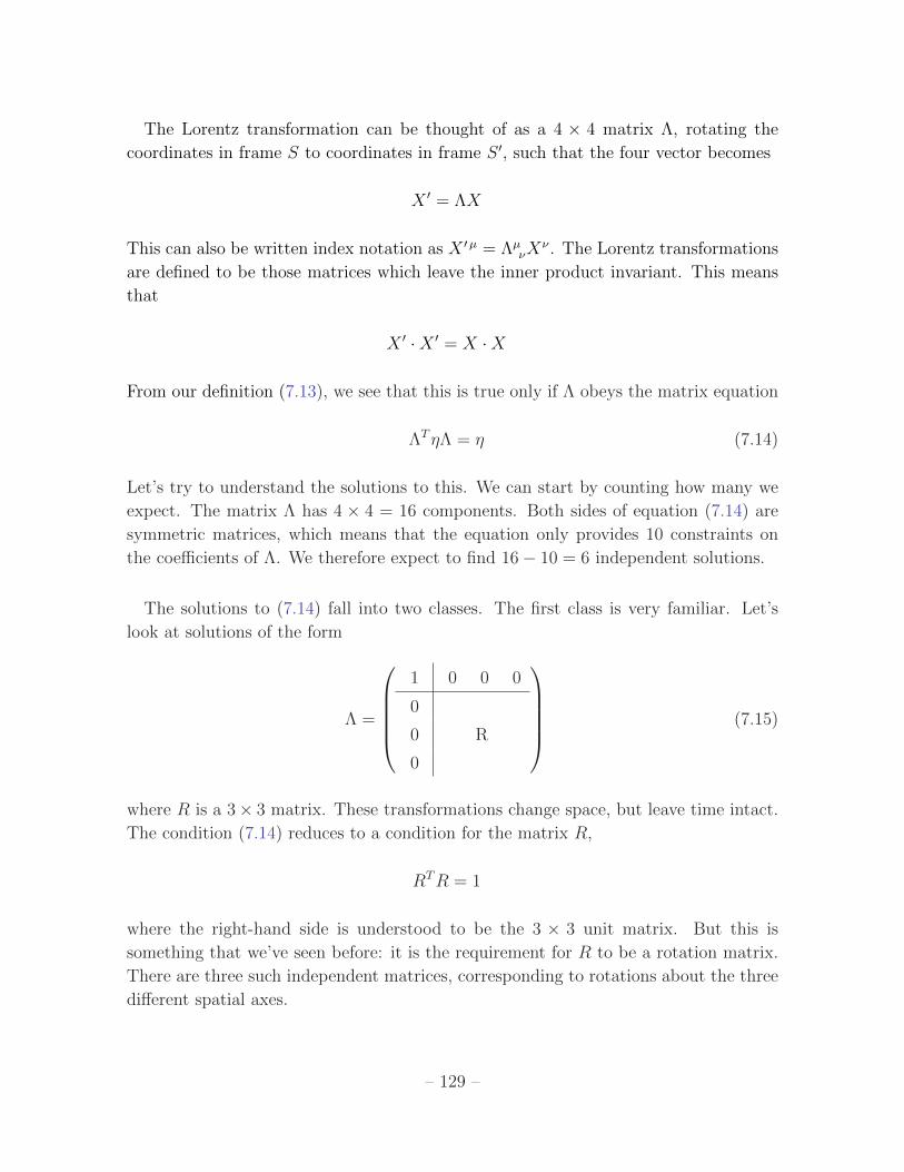
The Lorentz transformation can be thought of as a 4 × 4 matrix Λ, rotating the
coordinates in frame S to coordinates in frame S ′, such that the four vector becomes
X ′ = ΛX
This can also be written index notation as X ′µ = ΛµνX
ν . The Lorentz transformations
are defined to be those matrices which leave the inner product invariant. This means
that
X ′ ·X ′ = X ·X
From our definition (7.13), we see that this is true only if Λ obeys the matrix equation
ΛTηΛ = η (7.14)
Let’s try to understand the solutions to this. We can start by counting how many we
expect. The matrix Λ has 4 × 4 = 16 components. Both sides of equation (7.14) are
symmetric matrices, which means that the equation only provides 10 constraints on
the coefficients of Λ. We therefore expect to find 16− 10 = 6 independent solutions.
The solutions to (7.14) fall into two classes. The first class is very familiar. Let’s
look at solutions of the form
Λ =
1 0 0 0
0
0 R
0
(7.15)
where R is a 3× 3 matrix. These transformations change space, but leave time intact.
The condition (7.14) reduces to a condition for the matrix R,
RTR = 1
where the right-hand side is understood to be the 3 × 3 unit matrix. But this is
something that we’ve seen before: it is the requirement for R to be a rotation matrix.
There are three such independent matrices, corresponding to rotations about the three
different spatial axes.
– 129 –
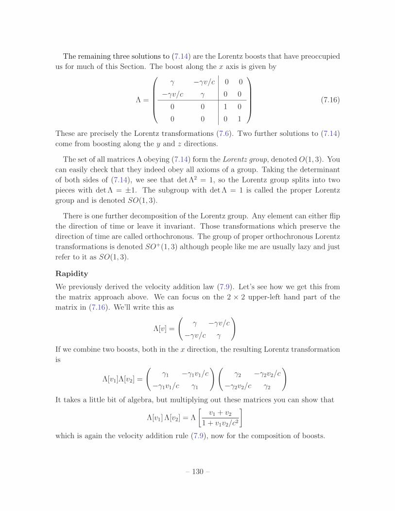
The remaining three solutions to (7.14) are the Lorentz boosts that have preoccupied
us for much of this Section. The boost along the x axis is given by
Λ =
γ −γv/c 0 0
−γv/c γ 0 0
0 0 1 0
0 0 0 1
(7.16)
These are precisely the Lorentz transformations (7.6). Two further solutions to (7.14)
come from boosting along the y and z directions.
The set of all matrices Λ obeying (7.14) form the Lorentz group, denoted O(1, 3). You
can easily check that they indeed obey all axioms of a group. Taking the determinant
of both sides of (7.14), we see that det Λ2 = 1, so the Lorentz group splits into two
pieces with det Λ = ±1. The subgroup with det Λ = 1 is called the proper Lorentz
group and is denoted SO(1, 3).
There is one further decomposition of the Lorentz group. Any element can either flip
the direction of time or leave it invariant. Those transformations which preserve the
direction of time are called orthochronous. The group of proper orthochronous Lorentz
transformations is denoted SO+(1, 3) although people like me are usually lazy and just
refer to it as SO(1, 3).
Rapidity
We previously derived the velocity addition law (7.9). Let’s see how we get this from
the matrix approach above. We can focus on the 2 × 2 upper-left hand part of the
matrix in (7.16). We’ll write this as
Λ[v] =
(γ −γv/c
−γv/c γ
)If we combine two boosts, both in the x direction, the resulting Lorentz transformation
is
Λ[v1]Λ[v2] =
(γ1 −γ1v1/c
−γ1v1/c γ1
)(γ2 −γ2v2/c
−γ2v2/c γ2
)It takes a little bit of algebra, but multiplying out these matrices you can show that
Λ[v1] Λ[v2] = Λ
[v1 + v2
1 + v1v2/c2
]which is again the velocity addition rule (7.9), now for the composition of boosts.
– 130 –
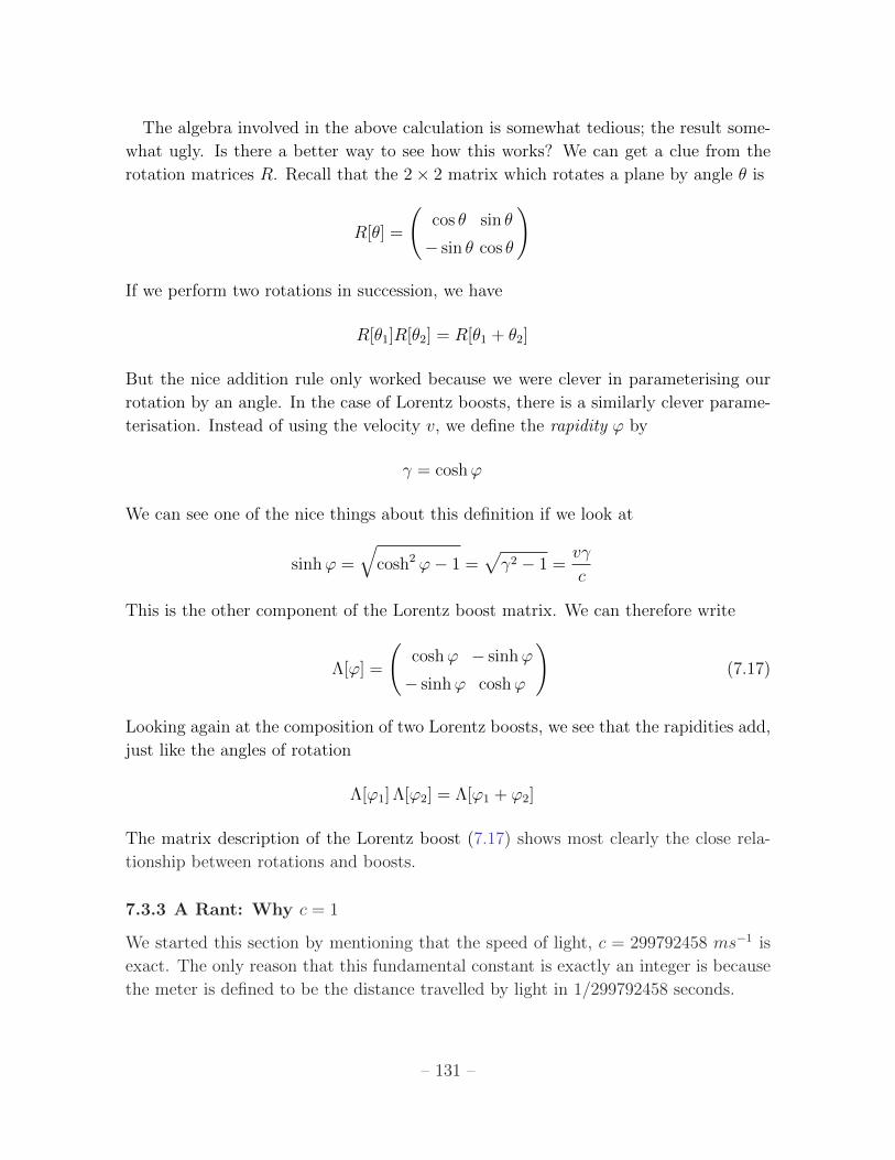
The algebra involved in the above calculation is somewhat tedious; the result some-
what ugly. Is there a better way to see how this works? We can get a clue from the
rotation matrices R. Recall that the 2× 2 matrix which rotates a plane by angle θ is
R[θ] =
(cos θ sin θ
− sin θ cos θ
)
If we perform two rotations in succession, we have
R[θ1]R[θ2] = R[θ1 + θ2]
But the nice addition rule only worked because we were clever in parameterising our
rotation by an angle. In the case of Lorentz boosts, there is a similarly clever parame-
terisation. Instead of using the velocity v, we define the rapidity ϕ by
γ = coshϕ
We can see one of the nice things about this definition if we look at
sinhϕ =
√cosh2 ϕ− 1 =
√γ2 − 1 =
vγ
c
This is the other component of the Lorentz boost matrix. We can therefore write
Λ[ϕ] =
(coshϕ − sinhϕ
− sinhϕ coshϕ
)(7.17)
Looking again at the composition of two Lorentz boosts, we see that the rapidities add,
just like the angles of rotation
Λ[ϕ1] Λ[ϕ2] = Λ[ϕ1 + ϕ2]
The matrix description of the Lorentz boost (7.17) shows most clearly the close rela-
tionship between rotations and boosts.
7.3.3 A Rant: Why c = 1
We started this section by mentioning that the speed of light, c = 299792458 ms−1 is
exact. The only reason that this fundamental constant is exactly an integer is because
the meter is defined to be the distance travelled by light in 1/299792458 seconds.
– 131 –

In our everyday world, the meter is a very useful unit. It is roughly the size of most
things in my house. But viewed from the perspective of fundamental physics, it is
rather parochial. If we’re going to pick the speed of light to be an integer, we should
probably pick one that is easier to remember. Like c = 1. We can do this by picking a
different unit of length, namely
c = 1 (light second) s−1
where a light second is the distance travelled by light in one second.
There’s a better way of thinking about this: the existence of a universal speed of light
is Nature’s way of telling us that space and time are more similar than our ancestors
realised. We only labelled space and time with different units because we were unaware
of the relationship between them.
We can illustrate this by going back to the rotational analogy. Suppose that you
decided that all distances in the x-direction should be measured in centimeters, while
all distances in the y-direction should be measured in inches. You then declared that
there was a new, fundamental constant of Nature – let’s call it λ – given by
λ ≈ 2.54 cm (inch)−1
Why is this a dumb thing to do? The reason it’s dumb is because of the rotational
symmetry of the laws of physics: different observers have different x and y coordinates
and can quite happily pick the same unit of measurement for both. But we’ve learned
in this section that there is also a symmetry between space and time. Insisting that we
retain the conversion factor c in the fundamental laws of physics is no more sensible
than retaining λ.
Despite my rant, in these lectures, we will retain c in all equations. (Although we
will use units which allow us to set λ = 1). But in future courses, it is common practice
to work with the convention c = 1. The equations look simpler and the only price you
pay is that the units of time and space are equivalent. If, at the end of the day, you
want to get your answer in terms of meters or seconds or whatever then you can always
put the factors of c back in by dimensional analysis.
7.4 Relativistic Kinematics
So far, our discussion has been focussed on what the world looks like to different
observers. Let’s now return to the main theme of these lectures: the motion of particles.
Remember that our ultimate goal is to construct laws of physics which look the same
– 132 –

to all inertial observers. For this reason, we will start by defining some of the basic
elements that go into the laws of physics: velocity, momentum and acceleration. We
want to define these in such a way that they have nice transformation properties when
viewed from different inertial frames.
7.4.1 Proper Time
We started these lectures in Section 1 by describing the trajectory of particle in an
inertial frame in terms of a curve x(t) and velocity u = dx/dt. There’s nothing incorrect
with this description in special relativity but, as we will see, there’s a much better way
to parameterise the trajectory of a particle.
Let’s start by considering a particle at rest at the origin of frame S ′ with x ′ = 0.
The invariant interval between two different points on the worldline of the particle is
∆s2 = c2∆t′ 2
We see that the invariant interval between two points on the worldline is proportional
to the time experienced by the particle. But this must be true in all frames. The time
experienced by the particle is called the proper time, τ . In all frames, it is given by
∆τ =∆s
c
where ∆s is real as long as the particle doesn’t travel faster than the speed of light, so
it sits on a timelike trajectory. (We keep promising to prove that a particle is unable
to travel faster than light...we are almost there!)
Proper time provides a way to parameterise the trajectory of a particle in a manner
that all inertial observers will agree on. Consider the trajectory of a general particle, not
necessarily travelling in a straight line. Viewed from an inertial frame S, the worldline
can be parameterised by x(τ) and t(τ). This has several advantages.
For example, we can use this formulation to determine the time experienced by a
particle moving along a general trajectory. Along a small segment of its trajectory, a
particle experiences proper time
dτ =
√dt2 − dx 2
c2= dt
√1− 1
c2
(dx
dt
)2
= dt
√1− u2
c2
from which we have
dt
dτ= γ (7.18)
– 133 –
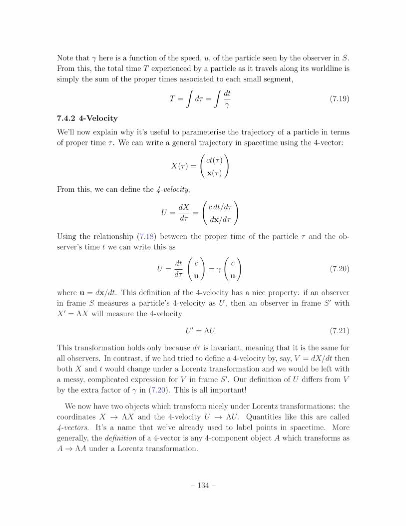
Note that γ here is a function of the speed, u, of the particle seen by the observer in S.
From this, the total time T experienced by a particle as it travels along its worldline is
simply the sum of the proper times associated to each small segment,
T =
∫dτ =
∫dt
γ(7.19)
7.4.2 4-Velocity
We’ll now explain why it’s useful to parameterise the trajectory of a particle in terms
of proper time τ . We can write a general trajectory in spacetime using the 4-vector:
X(τ) =
(ct(τ)
x(τ)
)From this, we can define the 4-velocity,
U =dX
dτ=
(c dt/dτ
dx/dτ
)
Using the relationship (7.18) between the proper time of the particle τ and the ob-
server’s time t we can write this as
U =dt
dτ
(c
u
)= γ
(c
u
)(7.20)
where u = dx/dt. This definition of the 4-velocity has a nice property: if an observer
in frame S measures a particle’s 4-velocity as U , then an observer in frame S ′ with
X ′ = ΛX will measure the 4-velocity
U ′ = ΛU (7.21)
This transformation holds only because dτ is invariant, meaning that it is the same for
all observers. In contrast, if we had tried to define a 4-velocity by, say, V = dX/dt then
both X and t would change under a Lorentz transformation and we would be left with
a messy, complicated expression for V in frame S ′. Our definition of U differs from V
by the extra factor of γ in (7.20). This is all important!
We now have two objects which transform nicely under Lorentz transformations: the
coordinates X → ΛX and the 4-velocity U → ΛU . Quantities like this are called
4-vectors. It’s a name that we’ve already used to label points in spacetime. More
generally, the definition of a 4-vector is any 4-component object A which transforms as
A→ ΛA under a Lorentz transformation.
– 134 –

Because of the simple transformation law (7.21), we can immediately import some of
the things that we learned from our previous discussion of Lorentz groups. In particular,
from the definition of Λ given in (7.14), we know that the inner product
U · U = UTηU
is invariant. It is the same for all observers: U · U = U ′ · U ′.
Let’s look at a simple example. A particle which is stationary in frame S has 4-
velocity
Uµ = (c, 0, 0, 0)
and so U · U = c2. But this must be true in all frames. We can check this explicitly
from (7.20) (we’ll take the middle equation to illustrate the point) which gives us
U · U =
(dt
dτ
)2 (c2 − u2
)=
(dt
dτ
)2c2
γ2= c2
This result also helps answer a puzzle. In Newtonian mechanics, if we want to specify
the velocity, we only have to give three numbers u. But in special relativity, the velocity
is a 4-vector U . Nonetheless, we still only need specify three variables because U is not
any 4-vector: it is constrained to obey U · U = c2.
Addition of Velocities Revisited
In Section 7.2.5, we derived the rule for the addition of velocities in one-dimension.
But what if the velocity of a particle is not aligned with the relative velocity between
S and S ′? The addition of velocities in this case is simple to compute using 4-vectors.
We start with a particle in frame S travelling with 4-velocity
U =
γuc
uγu cosα
uγu sinα
0
Here we’ve added the subscript to γu = (1 − u2/c2)−1/2 to distinguish it from the γ-
factor arising between the two frames. Frame S ′ moves in the x-direction with speed v
relative to S. The Lorentz boost is given in (7.16). In frame S ′, the 4-velocity is then
U ′ = ΛU = γu
(1− (uv/c2) cosα
)γvc
(u cosα− v)γv
u sinα
0
≡
γu′c
u′γu′ cosα′
u′γu′ sinα′
0
(7.22)
– 135 –

Dividing the t and x components of this 4-vector, we recover the velocity transformation
law (7.9) for the speed in the x-direction, namely
u′ cosα′ =u cosα− v
1− uv cosα/c2
Meanwhile, dividing the y component by the x component gives us a formula for the
angle α′ that the particles trajectory makes with the x′-axis,
tanα′ =u sinα
γv(u cosα− v)(7.23)
There is an interesting application of this formula to stellar aberration. The apparent
position of the stars changes over a 6 month period as the Earth moves around the
Sun. This is not due to difference in position of the Earth relative to the star: the
size of the Earth’s orbit is puny compared to the distance to the star. Instead, it is
a special relativistic effect, due to the motion of the Earth around the Sun. We can
derive this effect by applying the formulae above to light. Choose coordinate system
so that the position of the star — and hence the velocity of starlight — lies in the
(x, y) plane, while the Earth’s orbit lies in the (x, z) plane. Then we simply need to
substitute u = c in the above equation, while v is the component of the Earth’s velocity
in the x-direction.
The algebra can get somewhat messy, so it’s worth walking you through the steps.
It’s best to return to (7.22), now with u = u′ = c as befits a light ray. (It’s advisable
to first substitute the factor of γu′ in the x and y components for the expression for γu′
given in the temporal component). This then gives us
sinα′ =c sinα
γv(c− v cosα)and cosα′ =
c cosα− vc− v cosα
We now use the trig identity tan(α′/2) = sinα′/(1+cosα′). Substituting the expressions
above, a little algebra then results in the stellar aberration formula,
tanα′
2=
√c+ v
c− vtan
α
2
Here α is the angle that the star would appear at if the Earth was at rest. Or, said
another way, α is the angle at which the star appears at when the motion of the Earth
is perpendicular to the direction of the star. Meanwhile, α′ is the angle at which the
star appears when the Earth is travelling with speed v in the x-direction. As the Earth
moves around the Sun, the component of its velocity v in the x-direction changes,
meaning that the angle α′ at which the star appears also changes.
– 136 –
7.4.3 4-Momentum
The 4-momentum is defined by
P = mU =
(mcγ
mγu
)(7.24)
where m is the mass of the particle, usually referred to as the rest mass. Importantly,
it will turn out that P is the quantity that is conserved in the relativistic context. The
spatial components give us the relativistic generalisation of the 3-momentum,
p = mγu (7.25)
Notice that as the particle approaches the speed of light, u→ c, the momentum diverges
p → ∞. Since momentum is conserved in all processes, this is really telling us that
massive particles cannot break the speed of light barrier. (Here the word “massive”
doesn’t mean “really really big”: it just means “not massless”, or m 6= 0). This is
sometimes interpreted by viewing the quantity mγ as a velocity-dependent relativistic
mass. In these terms, the relativistic mass of the particle diverges mγ → ∞ as the
particle approaches the speed of light. The words may be different, but the maths (and
underlying physics) is the same: particles are bound by Nature’s speed limit. Nothing
can travel faster than the speed of light.
What is the interpretation of the time-component of the momentum 4-vector, P 0.
We can get a hint of this by Taylor expanding the γ factor,
P 0 =mc√
1− u2/c2=
1
c
(mc2 +
1
2mu2 + . . .
)(7.26)
The first term is just a constant. But the second term is something familiar: it is the
non-relativistic kinetic energy of the particle. This, coupled with the fact that all four
components of P are conserved, strongly suggests that the right interpretation of P 0 is
the energy of the particle (divided by c), so
P =
(E/c
p
)(7.27)
To show that P 0 is indeed related to the energy in this way requires a few more
techniques than we will develop in this course. The cleanest way is to use Noether’s
theorem – which we mentioned briefly in Section 5.1.4 – for relativistic systems and see
that P 0 is the quantity that follows from time translational invariance7.7You can read more about this for particle mechanics in the Classical Dynamics lecture notes
and, for relativistic field theories, in the Quantum Field Theory lecture notes. Both are available at
http://www.damtp.cam.ac.uk/user/tong/teaching.html
– 137 –

The expansion of (7.26) shows that both the mass and the kinetic energy contribute
to the energy of a particle. These combine to give
E = mγc2 (7.28)
Notice that as the particle approaches the speed of light, its energy diverges. Yet again,
we see a barrier to breaking the speed limit: as we approach the speed of light, the
energy required to make a particle go just a little faster gets bigger and bigger.
For a stationary particle, all its energy is contained in its rest mass, giving us the
famous slogan
E = mc2
There’s a nice way to rearrange (7.28), to replace the u in the γ factor with p defined
in (7.25). But the algebra is laborious. Instead there’s a cute trick that gives the result
much more quickly: we look at the inner product P ·P . In the rest frame of the particle,
P = (mc, 0, 0, 0) and we have
P · P = m2c2 (7.29)
But the inner product is an invariant, holding in any frame. From (7.27), we have
P · P =E2
c2− p 2
Equating these two expressions give
E2 = p 2c2 +m2c4 (7.30)
This is the generalisation of E = mc2 to include the kinetic energy. This equation can
also be derived the hard way by playing around with (7.28) and (7.25).
The identification P 0 = E/c has dramatic consequences. In Newtonian mechanics,
we boasted about the conservation of energy, but implicit in everything we did was the
more elementary fact that mass is conserved. Even in the variable mass problems of
Section 5.3, the mass never disappered: it just left our rocket ship. However, relativity
teaches us that the conservation of mass is subsumed into the conservation of energy.
There is nothing that guarantees that they are individually conserved. Just as potential
energy can be converted into kinetic energy, so too can mass be converted into kinetic
energy. In Japan, in 1945, this fact was vividly demonstrated.
– 138 –

7.4.4 Massless Particles
Until now, we built our discussion of particle trajectories on proper time. But, looking
back at Section 7.4.1, proper time is only defined for time-like trajectories. This is
fine for massive particles. But what about for massless particles? We can sidestep the
need for proper time by looking at the invariant of the 4-momentum (7.29) which, for
particles with m = 0, tells us that the 4-momentum must be null,
P · P = 0
This means that the 4-momentum of a massless particle necessarily lies along a light
ray.
This fact also allows us to clarify one of our original postulates of special relativity:
that the speed of light is the same for all inertial frames. You may wonder why the
propagation of light, an electromagnetic phenomenon, is singled out for special treat-
ment. The answer is: because the photon – the particle of light – is massless. In fact,
a better way of stating the postulate is to say that there is an upper speed limit in the
Universe, which is the same for all inertial observers. Any massless particle must travel
at this speed limit. All massive particles must go slower.
We know of only two types of massless particles in the Universe: the photon and the
graviton. Both of these owe their particle-like nature to quantum mechanics (actually,
this is true of all particles) and have a classical analog as light waves and gravity
waves respectively. You’ve all seen light waves (literally!) and individual photons have
been routinely measured in experiments for more than a century. In contrast there is
good, but indirect, evidence for gravity waves (this is expected to change soon, with
experiments up and running which are designed to directly detect gravity waves). There
appears to be no hope at all of detecting an individual graviton, at least within our
lifetimes.
Until the late 1990s, it was thought that neutrinos were also massless. It is now
known that they have a small, but finite mass. (Actually, there’s a caveat here: there
are three different types of neutrino: an electron neutrino, a muon neutrino and a tau
neutrino. The differences between their masses are known to be of order of 0.01 - 0.1 eV
and there are constraints which limit the sum of their masses to be no greater than
0.3 eV or so. But the absolute scale of their masses has not yet been determined. In
principle, one of the three neutrinos may be massless).
– 139 –

From (7.30), the energy and momentum of a massless particle are related by E2 =
p2c2. The four momentum takes the form
P =E
c
(1
p
)
where p is a unit vector in the direction of the particle’s motion.
To get an expression for the energy, we need a result from quantum mechanics which
relates the energy to the wavelength λ of the photon or, equivalently, to the angular
frequency ω = 2πc/λ,
E = ~ω =2π~cλ
There’s something rather nice about how this equation ties in with special relativity.
Suppose that in your frame, the photon has energy E. But a different observer moves
towards the light with velocity v. By the Lorentz transformation, he will measure the 4-
momentum of the photon to be P ′ = ΛP and, correspondingly, will see a bigger energy
E ′ > E. From the above equation, this implies that he will see a smaller wavelength.
But this is nothing other than Lorentz contraction.
The phenomenon of different observers observing different wavelengths of light is
called the Doppler effect. You will derive this in the problem sheet.
Tachyons and Why They’re Nonsense
It is sometimes stated that a particle which has imaginary mass, so that m2 < 0,
will have P · P < 0 and so travel consistently at speeds u > c. Such particles are
called tachyons. They too would be unable to cross Nature’s barrier at u = c and are
consigned to always travel on spacelike trajectories.
Although, consistent within the framework of classical relativistic particle mechanics,
the possibility of tachyons does not survive the leap to more sophisticated theories
of physics. All our current best theories of physics are written in the framework of
quantum field theory. Here particles emerge as ripples of fields, tied into small lumps
of energy by quantum mechanics. But in quantum field theory, it is not unusual to
have fields with imaginary mass m2 < 0. The resulting particles do not travel faster
than the speed of light. Instead, imaginary mass signals an instability of the vacuum.
– 140 –

7.4.5 Newton’s Laws of Motion
Finally, we are in a position to write down Newton’s law of motion in a manner that
is consistent with special relativity: it is
dP µ
dτ= F µ (7.31)
where F µ are the components of a 4-vector force. It is not difficult to anticipate that
the spatial components of F should be related to the 3-vector force f . (This is the same
thing that we’ve been calling F up until now, but we’ll lower its standing to a small f
to save confusion with the 4-vector). In fact, we need an extra factor of γ, so
F =
(F 0
γf
)
With this factor of γ in place, the spatial components of Newton’s equation (7.31) agree
with the form that we’re used to in the reference frame S,
dp
dt=dτ
dt
dp
dτ=
1
γ
dp
dτ= f
Similarly, a quick calculation shows that the temporal component F 0 is related to the
power: the rate of change of energy with time
F 0 =dP 0
dτ=γ
c
dE
dt
With these definitions, we can derive a familiar equation, relating the change in energy
to the work done. Consider a particle with constant rest mass m, so that P ·P = m2c2
is unchanging. Using P 0 = mγc and p = mγu, we have
d
dτ(P · P ) = 2P 0 dP
0
dτ− 2p · dp
dτ= 2γ2m
(dE
dt− u · f
)= 0
All of this is just to show how the familiar laws of Newtonian physics sit within special
relativity.
Electromagnetism Revisited
Ironically, equation (7.31) is rarely used in relativistic physics! The reason is that by
the time we are in the relativistic realm, most of the forces that we’ve come across are
no longer valid. The one exception is the electromagnetic force law for a particle of
– 141 –

charge q that we met in Section 2.4. This does have a relativistic formulation, with the
equation of motion given by
dP µ
dτ=q
cGµ
νUν
where Uν is the 4-velocity of the particle and Gµν is the electromagnetic tensor, a 4× 4
matrix which contains the electric and magnetic fields,
Gµν =
0 E1 E2 E3
E1 0 cB3 −cB2
E2 −cB3 0 cB1
E3 cB2 −cB1 0
(This tensor often goes by the name F µ
ν , but we’ve chosen to call it G to save confusion
with the force 4-vector). The spatial components of the four-vector equation gives rise
to the familiar Lorentz force law (2.19). The temporal component gives the rate of
work done, dE/dt = qE · u.
7.4.6 Acceleration
We can construct a four-vector for acceleration simply by
A ≡ dU
dτ
Note that because U · U = c2, we must have that A is always orthogonal to U in the
Minkowski sense: A · U = 0.
Suppose that the velocity of a particle in frame S is u. Then, in this frame, the
Newtonian notion of 3-acceleration is a = du/dt. Recalling our expression relating
time and proper time, dt/dτ = γ, we see that the four acceleration actually depends
on both u and a; it is
A = γ
(γc
γu + γa
)
with γ ≡ dγ/dt.
Let’s now suppose that we sit in an inertial frame S ′ in which, at a fixed moment of
time t, the particle is instantaneously at rest. Obviously, if the particle is accelerating,
– 142 –

this will not coincide with the particle’s rest frame an instant later, but momentarily
this will do fine. Since u′ = 0 in this frame, the 4-acceleration is
A′ =
(0
a′
)
with a′ = du′/dt′. (Note that you need to do a small calculation here to check that
γ(u = 0) = 0). But, since we have constructed our acceleration as a 4-vector, A and
A′ must be related by a Lorentz transformation. To make matters easy for ourselves,
let’s take both u and a to lie in the x-direction so that we can consistently ignore the
y and z-directions. Then the Lorentz transformation tells us
A = γ
(γc
γu+ γa
)=
(γ uγ/c
uγ/c γ
)(0
a′
)=
(uγa′/c
γa′
)
From the top component, we can determine the relationship between the accelerations
a and a′ seen in the two frames,
a ≡ u =(1− u2/c2
)3/2a′
Suppose now that the particle undergoes constant acceleration. As with everything
in special relativity, we need to be more careful about what we mean by this. The
natural interpretation is that the acceleration in the frame of the particle is constant.
Mathematically, this means that a′ is constant. In contrast, viewed from frame S, the
acceleration is not constant. Indeed, for constant a′, we can integrate our equation
above to get u, the velocity seen in frame S as a function of time. If we assume that
u = 0 when t = 0, we have
u =a′ct√
c2 + a′ 2t2⇒ γ(t) =
√1 +
a′ 2t2
c2(7.32)
Since u = x, integrating the first of these equations once more gives us the position in
the frame S as a function of time,
x =c
a′
(√c2 + a′ 2t2 − c
)(7.33)
where we’ve picked an integration constant so that x = 0 at time t = 0. We see that
the particle moves on the hyperbola shown in the figure. Viewed from S, the particle
approaches, but never reaches, the speed of light.
– 143 –

Notice that a particle at point P in the diagram
x
ct
P
Figure 56:
can only receive information from within its own past
lightcone, denoted by the red dotted lines in the figure.
However, if it continues along its accelerated trajectory,
it can never receive any information from the whole part
of spacetime to the left of the null line x = ct. This
part of the Universe will forever remain a mystery to an
accelerated observer. The null cone, defined by, x = ct,
which forms the boundary of the mysterious region is
called the Rindler event horizon. It has many things
in common with the event horizon of a black hole and,
indeed, the Rindler horizon is often used as a toy model to understand some of the
stranger aspects of black hole physics. Of course, if an accelerated observer really
wants to see what’s behind the horizon, it’s easy: he just stops accelerating. If an
observer in the background of a black hole wants to see what’s behind the horizon, he
must be somewhat braver.
We can look at what the accelerated observer feels. His time is simply the proper
time of the particle. To compute this, the form of γ(t) given in (7.32) is particularly
useful. From (7.19), if time t elapses in the stationary frame S, then the particle feels
τ =
∫ t
0
cdt√c2 + a′ 2t2
=c
a′sinh−1
(a′t
c
)This analysis gives us a more quantitative way to view
x
ct
Luke Leia
Figure 57:
the twin paradox. Suppose that Luke undertakes his
trip to Tatooine on a trajectory of constant acceleration.
He leaves Leia at the time t < 0 where their worldlines
intersects, arrives at Tatooine at t = 0 and x = c2/a′,
and returns back to Leia as shown. Leia experiences
time t; Luke time τ < t.
Finally, we can look at how far the accelerated ob-
server thinks he has travelled. Of course, this observer
is not in an inertial frame, but at any time t we can con-
sider the inertial frame that is momentarily at rest with
respect to the accelerated particle. This allows us to simply use the Lorentz contraction
formula. Using our results (7.32) and (7.33), we have
x′ =x
γ=c2
a′
(1− c√
c2 + a′ 2t2
)
– 144 –

Curiously, x′ → c2/a′ is finite as t → ∞ or, equivalently, as τ → ∞. Despite all that
effort, an accelerated observer doesn’t think he has got very far! This again, is related
to the presence of the horizon.
7.4.7 Indices Up, Indices Down
The minus signs in the Minkowski metric η means that it’s useful to introduce a slight
twist to the usual summation convention of repeated indices. For all the 4-vectors that
we introduced above, we were careful always place the spacetime index µ = 0, 1, 2, 3 as
a superscript (i..e up) rather than a subscript.
Xµ = (ct,x)
This is because the same object with an index down, Xµ, will mean something subtley
different!
Xµ = (ct,−x)
With this convention, the Minkowski inner product can be written using the usual
convention of summing over repeated indices as
XµXµ = c2t2 − x · x
In contrast, writing XµXµ = c2t2 +x2 is a dumb thing to write in the context of special
relativity since it looks very different to observers in different inertial frames. In fact,
we will shortly declare it illegal to write things like XµXµ.
There is a natural way to think of Xµ in terms of Xµ. If we write the Minkowski
metric as the diagonal matrix ηµν = diag(+1,−1,−1,−1) then we can raise and lower
indices using ηµν and the summation convention, so
Xµ = ηµνXν
Moreover, we will insist that all objects with indices up and down are similarly related
by contracting with η. For example, we could write the electromagnetic tensor as
Gµν = Gµρηρν =
0 −E1 −E2 −E3
E1 0 −cB3 cB2
E2 cB3 0 −cB1
E3 −cB2 cB1 0
The object Gµν is actually somewhat more natural than Gρ
ν since the former is anti-
symmetric.
– 145 –
To raise indices back up, we need the inverse of ηµν which, fortunately, is the same
matrix: ηµν = diag(+1,−1,−1,−1). We have
ηµρηρν = δµν
This trick of distinguishing between indices up and indices down provides a simple
formalism to ensure that all objects have nice transformation properties under the
Lorentz group. We insist that, just as in the usual summation convention, repeated
indices only ever appear in pairs. But now we further insist that pairs always appear
with one index up and the other down. The result will be an object with is invariant
under Lorentz transformations.
In future courses, you will learn that there is somewhat deeper mathematics lying
behind distinguishing Xµ and Xν : formally, these objects live in different spaces (some-
times called dual spaces). Objects such as Xµ are said to be covariant vectors, while
Xµ is said to be a contravariant vector.
7.5 Particle Physics
”Oh, that stuff. We never bother with that in our work”
Ernest Rutherford, the first particle physicist, discussing relativity
Our goal in this section is to describe various relativistic phenomena that arise in
particle physics. All these processes occur in the absence of external forces, so F = 0
and we will rely only on conservation of 4-momentum, meaning
dP
dτ= 0
Of course, conservation of 4-momentum includes both conservation of 3-momentum
and conservation of energy.
The calculations that follow are similar in spirit to the collision calculations of Section
5.2. Before we proceed, there are a couple of hints that may help when solving these
problems. Firstly, we need to choose a frame of reference in which to calculate: the
smart frame to choose is nearly always the centre of mass of the system. (Which should
more correctly be called the centre of momentum frame, for it is the one with vanishing
spatial 3-momentum). Secondly, you will often be presented with a situation where
there is one particle with momentum P about which you know nothing. A good way
to eliminate this is often to rearrange your equation so it takes the form P = . . . and
then square it to get the right-hand side to be P · P = m2c2. Let’s now see how this
works in a few examples.
– 146 –

7.5.1 Particle Decay
Consider a single particle with rest mass m1 which decays into two particles with rest
masses m2 and m3. Conservation of 4-momentum tells us
P1 = P2 + P3
or, equivalently,
E1 = E2 + E3 and p1 = p2 + p3
In the rest frame of the decaying particle, we can write (using (7.30)),
E1 = m1c2 =
√p2
2c2 +m2
2c4 +
√p2
3c2 +m2
3c4 ≥ m2c
2 +m3c2
which tells us the unsurprising result that a particle can only decay if its mass is greater
than that of its decay products. In the problem sheet, you will be asked to compute
the velocities v2 and v3 of the decay products in the centre of mass frame and show
that they are given by
γ2 =m2
1 +m22 −m2
3
2m1m2
and γ3 =m2
1 +m23 −m2
2
2m1m3
Here we will instead look at some slightly different problems.
An Example: Higgs Decay
The LHC has taught us that the Higgs boson has mass mhc2 ≈ 125 GeV . It mostly
decays into two photons. In particle physics, photons are always denoted by γ. Do
not confuse them with the Lorentz contraction factor! The “equations” in which the
photon γ’s appear are more like chemical reactions than true equations. The decay of
the Higgs into two photons is written as
h→ γγ
Similar decays occur for other particles, most notably the neutral pion, a meson (mean-
ing that it is made of a quark and anti-quark) with mass mπc2 ≈ 140 MeV . This too
decays as π0 → γγ.
To be concrete (and more relevant!) we’ll focus on the Higgs. Conservation of 4-
momentum tells us (in, hopefully, obvious notation) that
Ph = Pγ + P ′γ
If we sit in the rest frame of the Higgs, so P µh = (mhc, 0), the photons must have equal
and opposite 3-momentum, and therefore equal energy Eγ = 12mhc
2. The photons must
be emitted back-to-back but, because the problem is rotationally symmetric, can be
emitted at any angle.
– 147 –

What if we’re not sitting in the rest frame of the Higgs?. Suppose that the Higgs
has energy Eh and the energy of one of the photons is measured to be Eγ. What is the
angle θ that this photon makes with the path of the Higgs?
We’ll use the strategy that we described above. We have no information about the
second photon, with 4-momentum P ′γ. So we rearrange the conservation of momentum
to read P ′γ = Ph − Pγ. Upon squaring this, we have P ′γ · P ′γ = 0, so
0 = (Ph − Pγ) · (Ph − Pγ) = Ph · Ph + Pγ · Pγ − 2Ph · Pγ
= m2hc
2 − 2EhEγc2
+ 2ph · pγ
= m2hc
2 − 2EhEγc2
+2Eγc
cos θ√E2h/c
2 −m2hc
2
where, in the last equation, we have used E2 = p2c2 + m2c4 (which is just E = pc for
the photon). This can now be rearranged to give the answer for θ.
7.5.2 Particle Collisions
Let’s now look at the physics of relativistic collisions. We’ll collide two particles to-
gether, both of mass m. They will interact in some manner, preserving both energy
and 3-momentum, and scatter at an angle θ.
P1 + P2 = P3 + P4
As we mentioned previously, it’s easiest to see what happens in the centre of mass frame.
Without loss of generality, we’ll take the initial momenta to be in the x-direction. After
the collision, the particles must have equal and opposite momenta, which means they
must also have equal energy. This, in turn, ensures that in the centre of mass frame,
the speed v after the collision is the same as before. We can choose our axes so that
the initial and final momenta are given by
P µ1 = (mcγv,mvγv, 0, 0) , P µ
2 = (mcγv,−mvγv, 0, 0)
P µ3 = (mcγv,mvγv cos θ,mvγv sin θ, 0) , P µ
4 = (mcγv,−mvγv cos θ,−mvγv sin θ, 0)
where we’ve put the subscript on γv to denote its argument. We can also look at the
same collision in the lab frame. This refers to the situation where one of the particles is
initially at rest. (Presumably in your lab). By the velocity addition formula, the other
particle must start with speed
u =2v
1 + v2/c2
You can also derive this result by writing down the momenta P ′1 and P ′2 in the lab
frame and equating (P1 + P2)2 = (P ′1 + P ′2)2
– 148 –

θ
θ
φ
α
Figure 58: Collisions in the centre of mass frame on the left and the lab frame on the right
In the lab frame, the angles φ and α at which the particles scatter are not equal.
They can be easily determined using the addition of 4-velocities that we saw in Section
7.4.2 . Set u = −v in equation (7.23) and use the identity tan(x/2) = sin x/(1 + cos x)
to get
tanφ =1
γvtan θ/2 and tanα =
1
γvtan(θ/2 + π/2)
One of the more interesting examples of collisions is Compton Scattering, in which the
colour of light changes after scattering off an electron (because it changes its energy
and therefore its frequency). You will derive this result in the examples sheet.
Particle Creation
Just as mass can be converted into kinetic energy, so kinetic energy can be converted
into mass through the creation of new particles. Roughly speaking, this is the way we
discover new particles of Nature.
Suppose we collide two particles, each of mass m. After the collision, we hope to
be left with these two particles, together with a third of mass M . How fast must the
original two particles collide?
Conservation of momentum gives us
P1 + P2 = P3 + P4 + P5
where P 21 = P 2
2 = P 23 = P 2
4 = m2c2, while P 25 = M2c2. Let’s work in the centre of mass
frame of the colliding particles, each of which has speed v. In this case, we have
(P1 + P2)2 = 4m2γ2vc
2 = (P3 + P4 + P5)2 (7.34)
Since we’re in the centre of mass frame, the final momenta must take the form P3 +
P4 + P5 = ((E1 + E2 + E3)/c,0) so that
(P3 + P4 + P5)2 =1
c2(E1 + E2 + E3)2 ≥ 1
c2(2mc2 +Mc2)2
– 149 –
where, for each particle, we’ve used the fact that E =√m2c4 + p2c2 ≥ m2c2. Substi-
tuting this into (7.34) gives
4m2γ2vc
2 ≥ 4m2c2 +M2c2 + 4Mmc2 ⇒ γ ≥ 1 +M
2m(7.35)
This makes sense. The amount of minimum amount of kinetic energy per particle is
T = γmc2−mc2 = 12Mc2. With this minimum amount, the two colliding particles can
combine their kinetic energies to form the new particle. After the collision, all three
particles are then at rest.
It’s worth mentioning another way to do the above computation. Suppose that you
hadn’t noticed that the three-momentum of P3+P4+P5 vanished and instead expanded
out the right-hand side of (7.34) to end up with nine terms. Things are a bit harder
this way, but all is not lost. We can apply a Cauchy-Schwarz-like inequality to each of
these terms. For any massive particles with 4-momenta P and Q, such that P 2 = m21c
2
and Q2 = m22c
2, we necessarily have P · Q ≥ m1m2c2. It is simplest to prove this by
working in a frame in which one particle is stationary. Then we have
P ·Q =
(m1c
0
)·
(E2/c
p2
)= m1E2 = m1
√m2
2c4 + p2
2c2 ≥ m1m2c
2
Applied to (7.34) this once again gives (7.35).
What if we re-do this experiment in the lab frame, in which of the original particles is
at rest and the other has speed u? Now we have P1 = (mγuc,mγuu) and P2 = (mc, 0),
so
(P1 + P2)2 = P 21 + P 2
2 + 2P1 · P2 = 2m2c2 + 2m2γuc2
But we don’t have to compute (P3 + P4 + P5)2 again since the beauty of taking the
square of the 4-momenta is that the result is frame independent. We have
2m2c2 + 2m2γuc2 ≥ 4m2c2 +M2c2 + 4Mmc2 ⇒ γu ≥ 1 +
2M
m+M2
2m2
Now we see it’s not so easy to create a particle. It’s certainly not enough to give the
incoming particle kinetic energy T = 12Mc2 as one might intuitively expect. Instead,
if you want to create very heavy particles, M m, you need to give your initial
particle a kinetic energy of order T ≈ M2c2/2m. This scales quadratically with M ,
rather than the linear scaling that we saw in the centre of mass frame. The reason
for this simple: there’s no way that the end products can be at rest. The need to
– 150 –
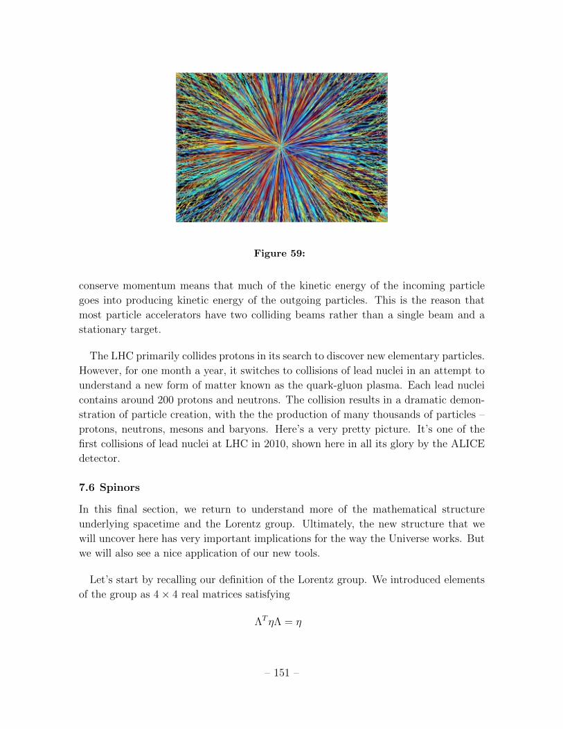
Figure 59:
conserve momentum means that much of the kinetic energy of the incoming particle
goes into producing kinetic energy of the outgoing particles. This is the reason that
most particle accelerators have two colliding beams rather than a single beam and a
stationary target.
The LHC primarily collides protons in its search to discover new elementary particles.
However, for one month a year, it switches to collisions of lead nuclei in an attempt to
understand a new form of matter known as the quark-gluon plasma. Each lead nuclei
contains around 200 protons and neutrons. The collision results in a dramatic demon-
stration of particle creation, with the the production of many thousands of particles –
protons, neutrons, mesons and baryons. Here’s a very pretty picture. It’s one of the
first collisions of lead nuclei at LHC in 2010, shown here in all its glory by the ALICE
detector.
7.6 Spinors
In this final section, we return to understand more of the mathematical structure
underlying spacetime and the Lorentz group. Ultimately, the new structure that we
will uncover here has very important implications for the way the Universe works. But
we will also see a nice application of our new tools.
Let’s start by recalling our definition of the Lorentz group. We introduced elements
of the group as 4× 4 real matrices satisfying
ΛTηΛ = η
– 151 –

where η = diag(1,−1,−1,−1) is the diagonal Minkowski metric. Elements with detΛ =
1 define the group SO(1, 3). If we further restrict to elements with the upper-left
component Λ00 > 0, which ensures that the transformation does not flip the direction
of time, then we have the sub-group SO+(1, 3). As we will now see, there’s some rather
beautiful subtleties associated with this group.
7.6.1 The Lorentz Group and SL(2,C)
The Lorentz group SO+(1, 3) is (almost) the same as the rather different looking group
SL(2,C), the group of 2× 2 complex matrices with determinant one. We will start by
providing the map between these two groups, and explaining what the word “almost”
means.
Before we talk about Lorentz transformations, let’s first go back to think about the
points in Minkowski space themselves. So far, we’ve been labelling these by the 4-
vector Xµ = (ct, x, y, z). But there is alternative way of labelling these points, not by
a 4-vector but instead by a 2× 2 Hermitian matrix. Given a 4-vector X, we can write
down such a matrix X by
X =
(ct+ z x− iyx+ iy ct− z
)
which clearly satisfies X = X†. Moreover, this is the most general form of a 2 × 2
Hermitian matrix. This means that there is a one-to-one map between 4-vectors X
and 2× 2 Hermitian matrices. We can equally well take the latter to define a point in
Minkowski space.
We learned earlier that Minkowski space comes equipped with an inner product
structure on 4-vectors. The inner product X · X measures the distance in spacetime
between the origin and the point X. But this is very natural in terms of the matrix
language: it is simply the determinant
X ·X = det X = c2t2 − x2 − y2 − z2
With this new way of labelling points in Minkowski space using the matrices X,
we can return to think about Lorentz transformations. Recall that, by definition, a
Lorentz transformation is a linear map which preserves the inner-product structure on
Minkowski space. Let’s consider a general matrix A ∈ SL(2,C). We can use this to
define a linear map
X → X ′ = AXA† (7.36)
– 152 –
By construction, if X = X† then we also have X ′ = (X ′)†, so X ′ also defines a point
in Minkowski space. Moreover,
det X ′ = det(AXA†) = detA detX detA† = detX
where the last equality follows because detA = 1. This means that the map (7.36)
preserves the inner product on Minkowski space and therefore defines a Lorentz trans-
formation.
We may wonder if all Lorentz transformations can be implemented by suitable choices
of A. The answer is yes. We’ll exhibit the map explicitly below, but first let’s just count
the dimension of the two groups to make sure we stand a chance of it working. A general
complex 2 × 2 matrix has 4 complex entries. The requirement that its determinant is
1 reduces this to 3 complex parameters, or 6 real parameters. This agrees with the
dimension of the Lorentz group: 6 = 3 rotations + 3 boosts.
Although the dimensions of SO+(1, 3) and SL(2,C) are equal, they are not quite the
same groups. In some sense, SL(2,C) is twice as big. The reason is that the matrices
A and −A both implement the same Lorentz transformation in (7.36). We say that
SL(2,C) is the double cover of SO+(1, 3) or, alternatively,
SO+(1, 3) ∼= SL(2,C)/Z2
Mathematically, there is a 2:1 group homomorphism between SL(2,C) and SO+(1, 3).
The word “homomorphism” means that the group structure is preserved under this
map. The existence of this double cover leads to some quite extraordinary consequences.
But, before we get to these, let’s first just look at how the map works in more detail.
Rotations
We’ve seen that points in Minkowski space can be written as a 4-vector X or Hermitian
matrix X. Meanwhile, Lorentz transformations act as X → ΛX or X → AXA†. Here
we would like to be more explicit about which matrices A correspond to the different
Lorentz transformations.
We start with rotations. By definition, these are the transformations which leave
time untouched. From (7.36), this means that we want matrices A which map X = ct 1
(where 1 here is the unit 2× 2 matrix) to itself. In other words, rotations should obey
AA† = 1
But such matrices are familiar unitary matrices. We learn that rotations sit in the
subgroup A ∈ SU(2) ⊂ SL(2,C). You may be used to thinking of the rotation group
– 153 –
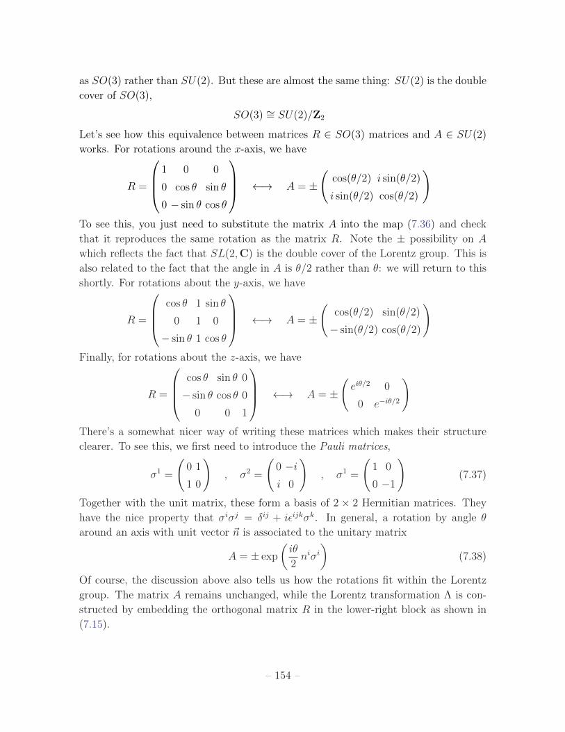
as SO(3) rather than SU(2). But these are almost the same thing: SU(2) is the double
cover of SO(3),
SO(3) ∼= SU(2)/Z2
Let’s see how this equivalence between matrices R ∈ SO(3) matrices and A ∈ SU(2)
works. For rotations around the x-axis, we have
R =
1 0 0
0 cos θ sin θ
0 − sin θ cos θ
←→ A = ±
(cos(θ/2) i sin(θ/2)
i sin(θ/2) cos(θ/2)
)
To see this, you just need to substitute the matrix A into the map (7.36) and check
that it reproduces the same rotation as the matrix R. Note the ± possibility on A
which reflects the fact that SL(2,C) is the double cover of the Lorentz group. This is
also related to the fact that the angle in A is θ/2 rather than θ: we will return to this
shortly. For rotations about the y-axis, we have
R =
cos θ 1 sin θ
0 1 0
− sin θ 1 cos θ
←→ A = ±
(cos(θ/2) sin(θ/2)
− sin(θ/2) cos(θ/2)
)
Finally, for rotations about the z-axis, we have
R =
cos θ sin θ 0
− sin θ cos θ 0
0 0 1
←→ A = ±
(eiθ/2 0
0 e−iθ/2
)
There’s a somewhat nicer way of writing these matrices which makes their structure
clearer. To see this, we first need to introduce the Pauli matrices,
σ1 =
(0 1
1 0
), σ2 =
(0 −ii 0
), σ1 =
(1 0
0 −1
)(7.37)
Together with the unit matrix, these form a basis of 2 × 2 Hermitian matrices. They
have the nice property that σiσj = δij + iεijkσk. In general, a rotation by angle θ
around an axis with unit vector ~n is associated to the unitary matrix
A = ± exp
(iθ
2niσi
)(7.38)
Of course, the discussion above also tells us how the rotations fit within the Lorentz
group. The matrix A remains unchanged, while the Lorentz transformation Λ is con-
structed by embedding the orthogonal matrix R in the lower-right block as shown in
(7.15).
– 154 –

Boosts
The Pauli matrices also provide a simple way to describe the A ∈ SL(2,C) corre-
sponding to Lorentz boosts. A boost with rapidity ϕ in the direction ~n is associated
to
A = ± exp(−ϕ
2niσi
)(7.39)
Unlike rotations, these matrices are not unitary. This ensures that they affect the time
component. Again, you can check that this reproduce the Lorentz boosts of the form
(7.17) simply by substituting this expression for A into the map (7.36). For example,
a boost in the z-direction is given by the matrix
A =
(e−ϕ/2 0
0 e+ϕ/2
)⇒ AXA† = X ′ =
(e−ϕ(t+ z) x− iyx+ iy e+ϕ(t− z)
)
This tells us that x and y are left unchanged, while t′ + z′ = e−ϕ(t + z) and t′ − z′ =
e+ϕ(t− z). Doing the algebra gives
t′ = coshϕ t− sinhϕ z , z′ = coshϕ z − sinhϕ t
which indeed agrees with the usual form of the Lorentz transformation (7.17) written
in terms of the rapidity.
7.6.2 What the Observer Actually Observes
There’s a rather nice application of the above formalism. In Section 7.2, when we
first encountered relativistic phenomena such as length contraction, we stressed that
different observers ascribe different coordinates to spacetime events. But this is not the
same thing as what the observer actually sees, for this also involves the time that the
light took to travel from the event to the observer. So this leaves open the question:
what does an observer observe? What do Lorentz contracted objects really look like?
As we will now show, writing the Lorentz group as SL(2,C) gives a wonderfully elegant
way to answer this question. Moreover, what we will find is somewhat surprising.
What an observer actually sees are, of course, light rays. As objects move through
Minkowski space, they emit light which then propagates to the position of the observer.
We’ve drawn this in the diagrams, both of which have the observer placed at the origin
of Minkowski space. We’ve also drawn the future and past lightcones emitted from the
origin.
– 155 –

t=0
celestialsphere
t’=0
celestialsphere
Figure 60: The celestial sphere for one
observer...
Figure 61: ...and for another
In the left-hand figure, the observer is assumed to be stationary with time coordinate
t. At each fixed moment in time, t, the light rays form a sphere S2. This is drawn as
the red circle in the past lightcone of the diagram. If we assume that no other object
comes between this sphere and the observer, then the light rays intersecting the sphere
are a good representation of what the observer actually sees. If he takes a snapshot of
everything around him with some really super-dooper fancy camera, he would record
the image on this sphere. This is sometimes given the name of the celestial sphere,
reflecting the fact that this is how we should think of viewing the night sky (at least if
the Earth wasn’t obscuring half of it).
Let’s now look at what an observer in a different inertial frame sees. This is shown
in the right-hand figure. This second observer will also take a snapshot using his fancy
camera as he passes through the origin. But this new observer’s celestial sphere is given
by null rays that sit at t′ = constant. Although it’s no longer obvious from the picture,
we know that the space defined by the intersection of light rays with the constant t′
hyperplane must still be a sphere simply because all inertial observers are equivalent.
However, this new celestial sphere is clearly tilted with respect to the previous one.
The four light rays drawn in the figure intersect both celestial spheres. These light
rays therefore provide a map between what the two observers see. This is a map
between the two celestial spheres, S2 → S2. Our goal is to construct this map.
This is where our new mathematical formalism comes in. Any point on a light ray is,
by definition, at vanishing distance from the origin when measured in the Minkowski
metric. Equivalently, the 2 × 2 Hermitian matrix X describing this point must have
vanishing determinant. But there’s a nice way to write down such matrices with zero
determinant. We introduce a two-component complex vector, ξα with α = 1, 2. Then
– 156 –
we write
X = ξξ† =
(|ξ1|2 ξ1ξ
†2
ξ2ξ†1 |ξ2|2
)
which, by construction, obeys det X = 0. It’s simple to check that the most general
Hermitian matrix X with det X = 0 can be written in this way. Note, however, that
there’s a redundancy in this description, since if we rotate both components of ξ by a
phase, so that ξ → eiβξ, then X remains unchanged.
An Aside: The Hopf Map
In our new notation, the celestial sphere at constant time t is simply given by
ξ†ξ = |ξ1|2 + |ξ2|2 = constant (7.40)
There’s actually some interesting maths in this statement. It’s obvious that given
two complex variables ξ1 and ξ2, the equation (7.40) defines a 3-dimensional sphere S3.
What’s perhaps less obvious, but nonetheless true, is that if we identify all points on S3
related by ξ → eiβξ, then we get a 2-dimensional sphere S2. In mathematical language,
we say that S3/U(1) ∼= S2.
It’s simple to write directly the map S3 → S2. Given a complex 2-vector, ξ, obeying
ξ†ξ = 1, you can define 3 real numbers ki by
ki = ξ†σiξ
where σi are the three Pauli matrices (7.37). Then a little algebra shows that kiki = 1.
In other words, ki gives a point on S2. This is map from S3 to S2 is called the Hopf
map.
Back to the Real World
Let’s now use these new objects ξ to construct the map between the two celestial
spheres. A nice fact is that Lorentz transformations act in a natural way on the two-
component ξ. To see this, recall that
X ′ = ξ′ξ′† = Aξξ†A†
But we can view this as a transformation of ξ itself. We have simply the SL(2,C)
transformation
ξ′ = Aξ (7.41)
– 157 –

Figure 62: The stereographic projection. The southern hemisphere is mapped to inside the
dotted circle; the northern hemisphere is mapped to outside this circle.
However, this is not quite our mapping. We can start with a celestial sphere defined
by (7.40) and act with a Lorentz transformation. The trouble is that the resulting
space we get remains the first celestial sphere, just written in the second observer’s
coordinates. We still need to propagate the light rays forward and backwards so that
they intersect the second celestial sphere.
To avoid this complication, it’s best to think about these celestial spheres in a slightly
different way. Rather than saying that they are defined at constant time, let’s instead
define them as equivalence classes of light rays. This means that we lose the information
about where we are along the light ray: we only keep the information about which light
ray we’re talking about. Mathematically, this is very simple: to each ξ we associate a
single complex number ω ∈ C by
ω =ξ1
ξ2
The map from the celestial sphere S2 → C is known as stereographic projection and
is shown in the figure. Strictly speaking, ω parameterises C ∪ ∞, with the point
at infinity included to accommodate the point ξ2 = 0, which is the North pole of the
celestial sphere. This extended complex plane is called the Riemann sphere.
Now the light rays seen by the first observer are labelled by ω ∈ C and form a
celestial sphere. The light rays seen by the second observer are labelled by ω′ = ξ′1/ξ′2
and form a different celestial sphere. A Lorentz transformation A ∈ SL(2,C) acts on
ξ as (7.41) which, in terms of ω, reads
ω′ =aω + b
cω + dwhere A =
(a b
c d
)and ad− bc = 1 (7.42)
– 158 –

This transformation on the complex plane is known as a Mobius transformation. It’s
simple to see that Mobius transformations form a group. In fact, from what we’ve seen
above, you shouldn’t be surprised to learn that the group of Mobius transformations is
SL(2,C), up to a discrete Z2 identification.
Suppose now that the first observers sees an object on his celestial sphere that traces
out some shape. After stereographic projection, that will result in a shape on the
complex plane (perhaps passing through the point at infinity). This appears to the
second observer to be transformed by (7.42). Upon taking the inverse stereographic
projection, we will learn what shape the second observer really sees.
To make progress, we should look at a simple example. And the simplest example is
for an object which is itself a sphere. This means that, when stationary with respect
to the first observer, the outline of the object looks like a circle. What does the second
observer see? To answer this, I’ll need to invoke some simple facts about stereographic
projection and Mobius transformations. Although I won’t prove them, they are among
the most basic properties of these transformations and will be proven in next year’s
Geometry course. The facts are:
• The stereographic projection maps circles on the sphere to circles or lines on the
plane.
• Mobius transformations map circles and lines on the plane to circles or lines on
the plane.
Hiding behind these facts is the statement that both maps are conformal, meaning that
they preserve angles. But, for us, the upshot is that a circle on the first celestial sphere
is mapped under a Lorentz transformation to a circle on the second.
Let’s pause to take this in. The first observer saw an object which had the shape
of a circle. Based on the arguments of Lorentz contraction, you might expect that the
second observer sees a squashed circle, maybe an ellipse. Yet this is not what happens.
Instead, the second observer also sees a circle! The effects of the time of flight of
light completely eliminate the Lorentz contraction. This fact was only realised more
than 50 years after Einstein’s formulation of special relativity when it was discovered
independently by Terrell and Penrose. It is sometimes said to be the “invisibility of the
Lorentz contraction”. Note that it doesn’t mean that the effects of Lorentz contraction
that we discussed before are not real. It just means that you don’t get to see them if
you take a picture of a sphere. Moreover, if you look more closely you find that there
are things that change. For example, if you paint a picture on the surface of the sphere,
this will appear deformed to the other observer.
– 159 –

7.6.3 Spinors
Finally, we’re in a position to explain what the title of this section means. A spinor
is simply a two-dimensional complex vector ξ which, under a Lorentz transformation
A ∈ SL(2,C), changes as ξ → Aξ.
(Some confusing caveats: ξ defined in this way is known as a Weyl spinor. In fact,
strictly speaking, it is known as a left-handed Weyl spinor. For reasons that I won’t go
into here, we can also define something called a right-handed Weyl spinor by exchanging
ϕ → −ϕ in the definition of the boosts (7.39). Then combining a left-handed Weyl
spinor together with a right-handed Weyl spinor gives a four component complex object
that is called a Dirac Spinor. See, I told you it would be confusing!)
We’ve already seen how spinors can be used to describe light rays. But this is not
their only use; they have much more a life of their own. Before I describe this, let
me firstly explain a property that makes it very surprising that spinors have any real
relevance in the world. This harks back to the observation that SL(2,C) is the double
cover of the Lorentz group. Suppose that there is some object in the Universe that is
actually described by a spinor. This means, in particular, that the state of the object
with ξ is different from the state of the object with −ξ. What happens when we rotate
this object? Well, we’ve already seen how to enact a rotation using SL(2,C) matrices:
they are given by (7.38). Except if we’re acting on spinors we need to make a decision:
do we pick +A or do we pick −A? Because, unlike the action on Minkowski space,
these two different matrices will result in different states ξ after a rotation. It doesn’t
actually matter which choice we pick, as long as we make one. So let’s decide that a
rotation about an axis ni acts on a spinor by
ξ → exp
(iθ
2niσi
)ξ
This all seems fine. The surprise comes when we look at what happens if we rotate the
spinor by 2π. It doesn’t come back to itself. Instead, after a rotation by 2π we find
ξ → −ξ. We have to rotate by 4π to get the spinor to return to itself!
Wouldn’t it be astonishing if there were objects in the Universe which had this
property: that you could rotate them and find that they didn’t come back to themselves.
This is even more astonishing when you realise that rotating an object is the same thing
as walking around it. If such objects existed, you would be able to circle them once
and see that the object sits in a different state just because you walked around it. How
weird would that be?
– 160 –

Well, such objects exist. What’s more, they’re the same objects that you and I
are made of: electrons and protons and neutrons. All of these particles carry a little
angular momentum whose direction is described by a spinor rather than a vector. This
means that Nature makes use of all the pretty mathematics that we’ve introduced in
this section. The symmetry group of the Universe we live in is not the Lorentz group
SO+(1, 3). Instead, it is the double cover SL(2,C). And the basic building blocks of
matter have subtle and wonderful properties. Turn an electron 360o and it isn’t the
same; turn it 720o and you’re back to where you started. If you want to learn more
about this, you can find deeper explanations in the lecture notes on Quantum Field
Theory.
– 161 –