Dynamic topography, phase boundary topography and latent-heat release

Bernhard Steinberger

Center for Geodynamics, NGU, Trondheim, Norway

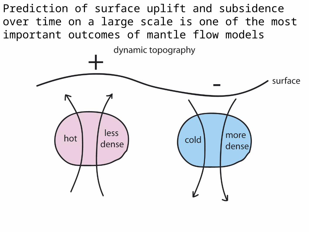
Prediction of surface uplift and subsidence over time on a large scale is one of the most important outcomes of mantle flow models

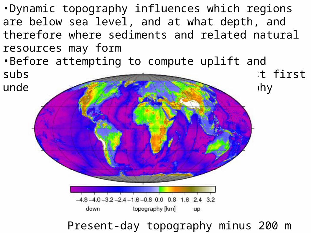
•Dynamic topography influences which regions are below sea level, and at what depth, and therefore where sediments and related natural resources may form•Before attempting to compute uplift and subsidence in the geologic past, we must first understand present-day dynamic topography

Present-day topography

•Dynamic topography influences which regions are below sea level, and at what depth, and therefore where sediments and related natural resources may form•Before attempting to compute uplift and subsidence in the geologic past, we must first understand present-day dynamic topography

Present-day topography + 200 m

•Dynamic topography influences which regions are below sea level, and at what depth, and therefore where sediments and related natural resources may form•Before attempting to compute uplift and subsidence in the geologic past, we must first understand present-day dynamic topography

Present-day topography minus 200 m

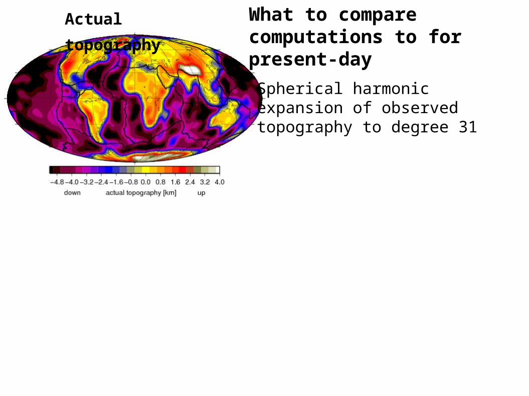
Actual topography

Spherical harmonicexpansion of observed topography to degree 31

What to compare computations to for present-day

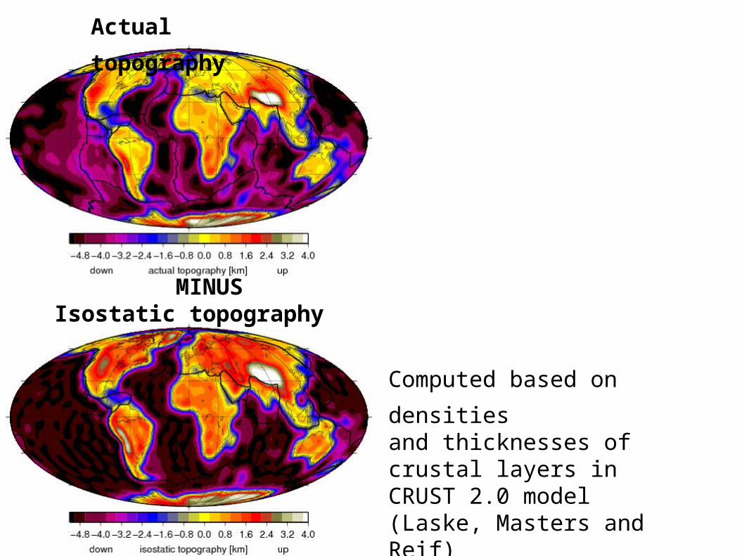
Actual topography

MINUSIsostatic topography

Computed based on densities and thicknesses of crustal layers inCRUST 2.0 model(Laske, Masters and Reif)http://mahi.ucsd.edu/Gabi/rem.html

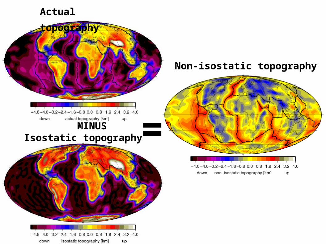
Actual topography

MINUSIsostatic topography

Non-isostatic topography

=

Non-isostatic topography

Non-isostatic topography

MINUSThermal topography

Computed from the age_2.0 ocean floor age grid (Müller, Gaina, Sdrolias and Heine, 2005) for ages < 100 Ma

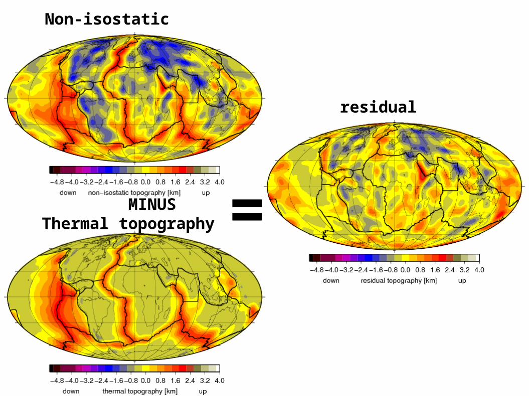
Non-isostatic topography

residual topography

MINUSThermal topography =

residual topography, l=1-31

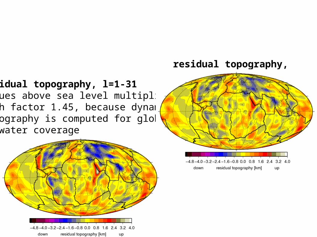
residual topography, l=1-31

residual topography, l=1-31Values above sea level multipliedwith factor 1.45, because dynamictopography is computed for globalseawater coverage

residual topography, l=1-12, above sea level mulitiplied with 1.45

residual topography, l=1-31

residual topography, l=1-31 Above sea level multiplied with 1.45

residual topography, l=1-12

RMS amplitude 0.52 km

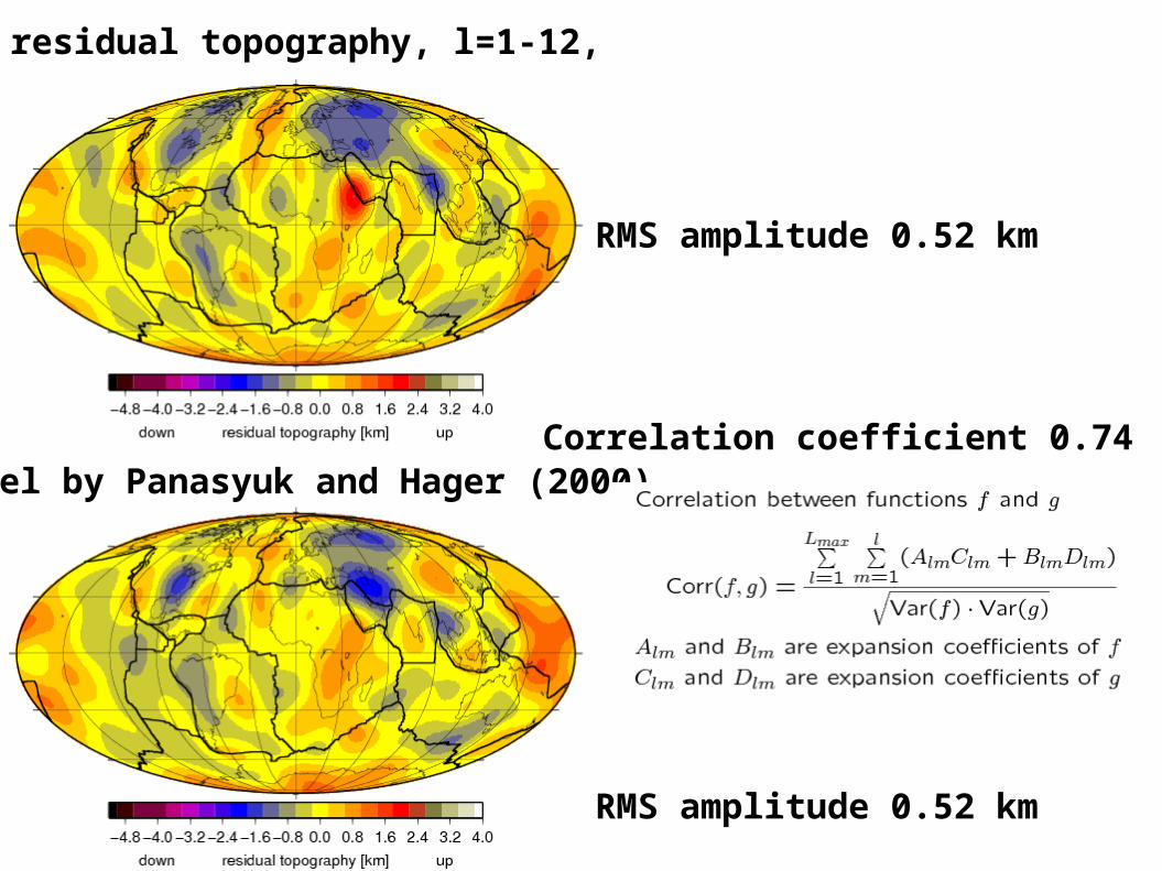
residual topography, l=1-12, our model

RMS amplitude 0.52 km

Model by Panasyuk and Hager (2000)

RMS amplitude 0.52 km

Correlation coefficient 0.74

residual topography, l=1-12, our model

RMS amplitude 0.52 km

Model by Kaban et al. (2003)

RMS amplitude 0.64 km

Correlation coefficient 0.86

Positive Clapeyron slope

Radial stress kernels Kr,l(z) describe how much a density anomaly lmat a depth z contributes to dynamic topography:

Computed for global water coverage: s= 2280 kg/m3

Figure from Steinberger, Marquart and Schmeling (2001)

l=2

l=31

l=2

l=31

l=2

l=31

l=2

l=31

Kr,l(z)

•Densities inferred from S-wave tomography -- here: model S20RTS (Ritsema et al., 2000)•Conversion factor ~ 0.25 (Steinberger and Calderwood, 2006) – 4 % velocity variation ~~ 1 % density variation

Depth 300 km

4.8 4.0 3.2 2.4 1.6 0.8 0.0 -0.8 -1.6 -2.4 -3.2 -4.0

•Densities inferred from S-wave tomography -- here: model S20RTS (Ritsema et al., 2000) •Disregard velocity anomalies above 220 km depth

Depth 200 km

4.8 4.0 3.2 2.4 1.6 0.8 0.0 -0.8 -1.6 -2.4 -3.2 -4.0

Dynamic topography •Spectral method (Hager and O’Connell, 1979,1981) for computation of flow and stresses•NUVEL plate motions for surface boundary condition (results remain similar with free-slip and no-slip surface)•Radial viscosity variation only

RMS amplitude 1.07 kmWith other tomography models:0.63 km [Grand] to 1.47 km [SB4L18, Masters et al., 2000]

Viscosity profile fromSteinberger and Calderwood (2006)

Dynamic topographyRMS amplitude 1.07 km With other tomography models:0.63 to 1.47 km

Correlation 0.33With other tomography models:0.30 to 0.53

Residual topography RMS amplitude 0.52 kmOther models: 0.47 to 0.64 km

Predicted “410” topography Thermal effect onlyRMS amplitude 4.81 kmWith other tomography models: 2.85 to 7.43 km

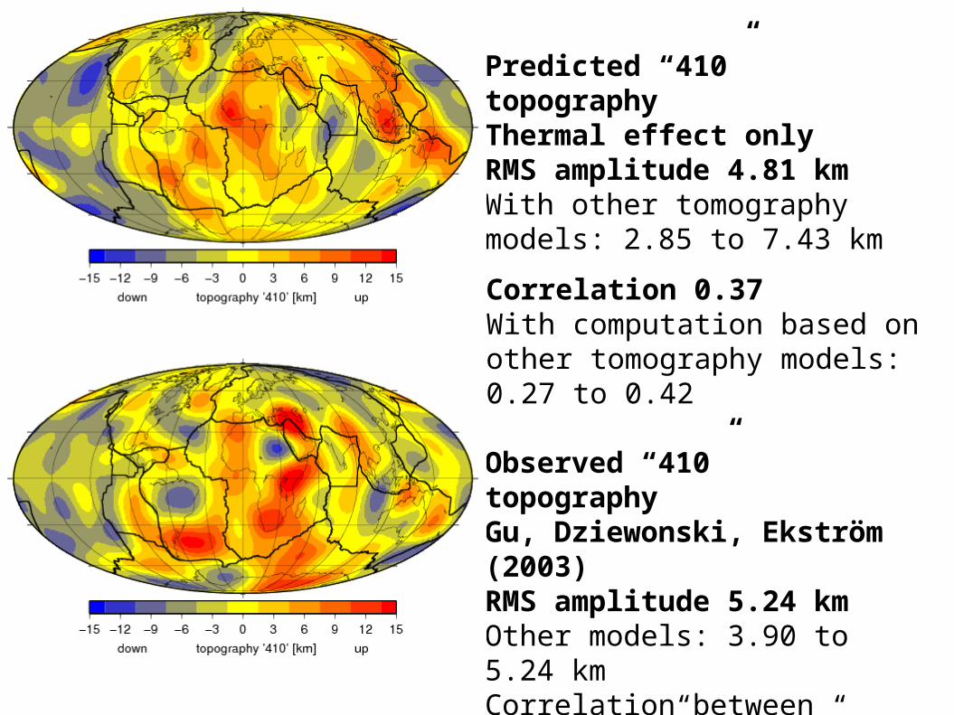
Predicted “410” topography Thermal effect onlyRMS amplitude 4.81 kmWith other tomography models: 2.85 to 7.43 km

Observed “410” topographyGu, Dziewonski, Ekström (2003)RMS amplitude 5.24 kmOther models: 3.90 to 5.24 kmCorrelation between different ”observed” models 0.10 to 0.44

Correlation 0.37With computation based on other tomography models:0.27 to 0.42

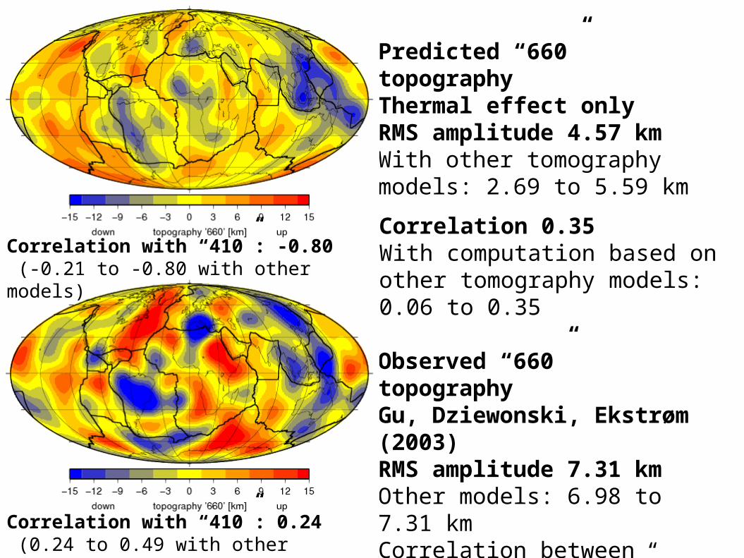
Predicted “660” topography Thermal effect onlyRMS amplitude 4.57 kmWith other tomography models: 2.69 to 5.59 km

Observed “660” topographyGu, Dziewonski, Ekstrøm (2003)RMS amplitude 7.31 kmOther models: 6.98 to 7.31 kmCorrelation between different “observed” models 0.33 to 0.50

Correlation 0.35With computation based on other tomography models:0.06 to 0.35

Correlation with “410”: -0.80 (-0.21 to -0.80 with other models)

Correlation with “410”: 0.24 (0.24 to 0.49 with other models)

Predicted TZ thickness variationThermal effect onlyRMS amplitude 8.89 kmWith other tomography models: 5.05 to 11.86 km

Observed TZ thickness variationGu, Dziewonski, Ekstrøm (2003)RMS amplitude 7.92 kmOther models: 6.52 to 7.92 kmCorrelation between different “observed” models 0.30 to 0.41

Correlation 0.51With computation based on other tomography models:0.36 to 0.51

Dynamic topography – correlation with predicted TZ thickness variation –0.77With other tomography models: -0.48 to –0.89

Residual topography - correlationwith observed TZ thickness variation –0.17Other models: -0.17 to 0.02

Summary of results with thermal effect only:

Summary of results with thermal effect only:

•Predicted dynamic topography bigger than observed

Summary of results with thermal effect only:

•Predicted dynamic topography bigger than observed

•Predicted topography “660” smaller than observed

Summary of results with thermal effect only:

•Predicted dynamic topography bigger than observed

•Predicted topography “660” smaller than observed

•“410” and “660” topography correlation predicted negative, observed positive

Summary of results with thermal effect only:

•Predicted dynamic topography bigger than observed

•Predicted topography “660” smaller than observed

•“410” and “660” topography correlation predicted negative, observed positive

•TZ thickness and dyn. topography correlation predicted negative, obs. ~ zero

Summary of results with thermal effect only:

•Predicted dynamic topography bigger than observed

•Predicted topography “660” smaller than observed

•“410” and “660” topography correlation predicted negative, observed positive

•TZ thickness and dyn. topography correlation predicted negative, obs. ~ zero

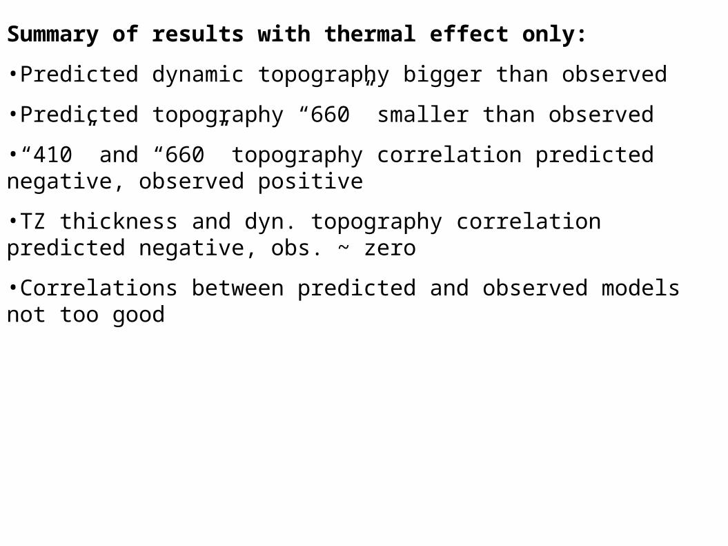
•Correlations between predicted and observed models not too good

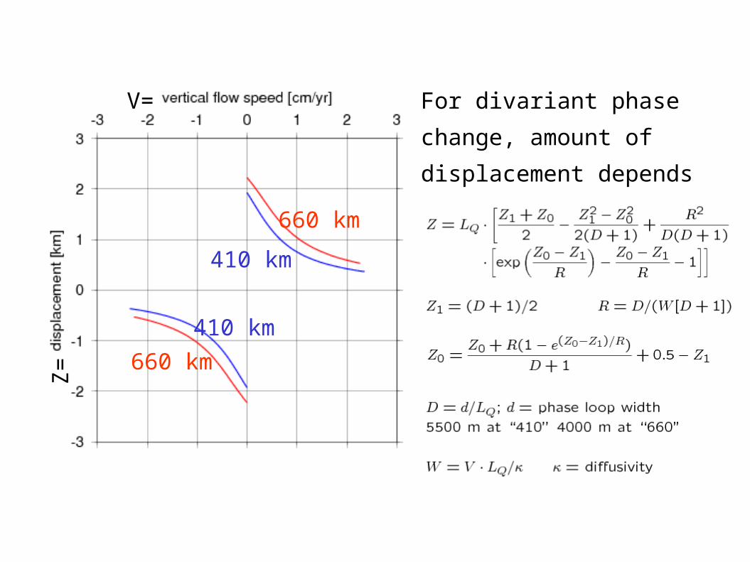
410 km: Phase boundary with positive Clapeyron slope

Latent heat causes HIGHER temperature BELOW

Phase boundary topography by latent

heat effects (Christensen, 1998, EPSL)

660 km: Phase boundary with negative Clapeyron slope

Latent heat causes LOWER temperature BELOW

In both cases:

Temperature gradient on upstream side

Constant temperature on downstream side

Boundary displaced in direction of flow

410 km: Phase boundary with positive Clapeyron slope

Latent heat causes HIGHER temperature BELOW

660 km: Phase boundary with negative Clapeyron slope

Latent heat causes LOWER temperature BELOW

In both cases:

Temperature gradient on upstream side

Constant temperature on downstream side

Boundary displaced in direction of flow

Phase boundary topography by latent

heat effects (Christensen, 1998, EPSL)

LQ = g cp) = 3.8 km cp = specific heat capacity

LQ = 4.4 km

For divariant phase change,

amount of displacement depends

on flow speed

410 km

410 km

660 km

660 km

For divariant phase change,

amount of displacement depends

on flow speed

410 km

410 km

660 km

660 km

V=

Z=

Computed flow speed – Depth 410 km

Computed flow speed – Depth 660 km

Density model inferred from S20RTS (Ritsema et al., 2000)

depth 660 km

Phase boundary displacement due to latent heat– depth 410 km

“660” phase boundary displacement

Thermal effect

Latent heat effect

•Predicted topography “660” smaller than observed•Increases by including latent heat effect (but not enough – note different scale!)

depth 660 km

Phase boundary displacement due to latent heat– depth 410 km

•“410” and “660” topography correlation predicted negative, observed positive•Latent heat effect displaces phase boundaries in same direction and hence contributes towards less negative correlation (but not enough – note different scale!)

depth 660 km

Phase boundary displacement due to latent heat – depth 410 km

Effect of latent heat effect on dynamic topography

Effect of latent heat effect on dynamic topography

Dynamic topography with thermal effect only

•Computed dynamic topography bigger than observed•Including latent heat effect reduces dynamic topography (note opposite sense of color scale! - but not enough – note different scale)

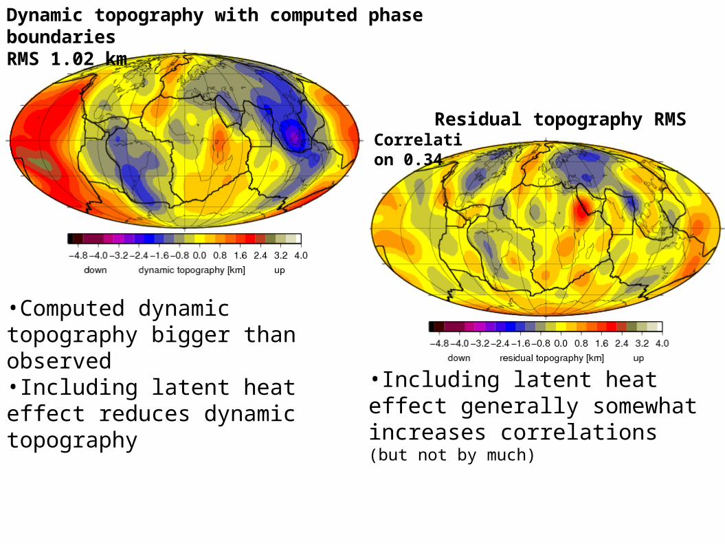
Residual topography RMS 0.52 km

•Computed dynamic topography bigger than observed•Including latent heat effect reduces dynamic topography •Including latent heat effect

generally somewhat increases correlations (but not by much)

Correlation 0.34

Dynamic topography with computed phase boundariesRMS 1.02 km

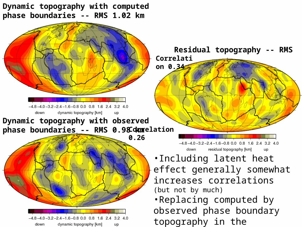
Residual topography -- RMS 0.52 km

•Including latent heat effect generally somewhat increases correlations (but not by much)

•Replacing computed by observed phase boundary topography in the calculation of dynamic topography generally does not improve results

Correlation 0.34

Dynamic topography with computed phase boundaries -- RMS 1.02 km

Dynamic topography with observed phase boundaries -- RMS 0.98 km Correlation

0.26

Combine dynamic topography with sea level curve to compute

inundation

Heine et al., in

preparation

Present-day

64 Ma

41 Ma

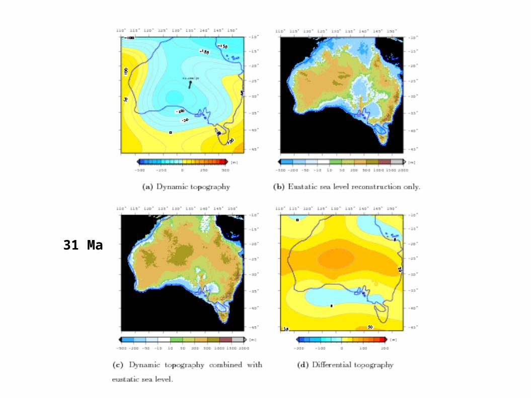
31 Ma

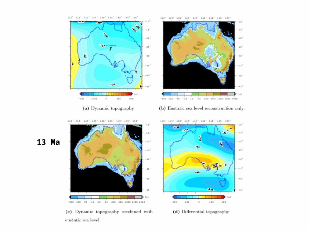
13 Ma

8 Ma

3 Ma

Dynamic topography on New Jersey Margin

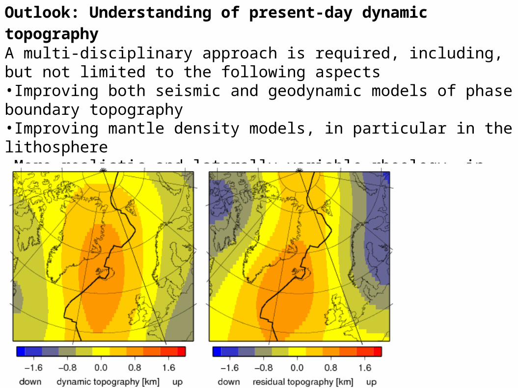
Outlook: Understanding of present-day dynamic topography A multi-disciplinary approach is required, including, but not limited to the following aspects•Improving both seismic and geodynamic models of phase boundary topography•Improving mantle density models, in particular in the lithosphere•More realistic and laterally variable rheology, in particular in the lithosphere•Regional computations

Outlook II: Time-dependent dynamic topography and plate motions

•Past mantle structure cannot be fully recovered by simple backward-advection•A global mantle reference frame through geologic times is required to relate computed uplift and subsidence to geological observations