Embed Size (px)
Citation preview
Journal of Machine Learning Research 22 (2021) 1-35 Submitted 9/19;Revised 12/20; Published 2/21
Dynamic Tensor Recommender Systems
Yanqing Zhang [email protected]
Department of Statistics
Yunnan University
Kunming, 650504, China
Xuan Bi [email protected]
Carlson School of Management
University of Minnesota
Minneapolis, MN, 55455-0438, USA
Niansheng Tang [email protected]
Department of Statistics
Yunnan University
Kunming, 650504, China
Annie Qu [email protected]
Department of Statistics
University of California
Irvine, CA, 92697-3425, USA
Editor: Animashree Anandkumar
Abstract
Recommender systems have been extensively used by the entertainment industry, busi-ness marketing and the biomedical industry. In addition to its capacity of providingpreference-based recommendations as an unsupervised learning methodology, it has beenalso proven useful in sales forecasting, product introduction and other production relatedbusinesses. Since some consumers and companies need a recommendation or predictionfor future budget, labor and supply chain coordination, dynamic recommender systemsfor precise forecasting have become extremely necessary. In this article, we propose a newrecommendation method, namely the dynamic tensor recommender system (DTRS), whichaims particularly at forecasting future recommendation. The proposed method utilizes atensor-valued function of time to integrate time and contextual information, and createsa time-varying coefficient model for temporal tensor factorization through a polynomialspline approximation. Major advantages of the proposed method include competitive fu-ture recommendation predictions and effective prediction interval estimations. In theory,we establish the convergence rate of the proposed tensor factorization and asymptotic nor-mality of the spline coefficient estimator. The proposed method is applied to simulations,IRI marketing data and Last.fm data. Numerical studies demonstrate that the proposedmethod outperforms existing methods in terms of future time forecasting.
Keywords: Contextual information, Dynamic recommender systems, Polynomial splineapproximation, Prediction interval, Product sales forecasting
c©2021 Yanqing Zhang, Xuan Bi, Niansheng Tang and Annie Qu.
License: CC-BY 4.0, see https://creativecommons.org/licenses/by/4.0/. Attribution requirements are providedat http://jmlr.org/papers/v22/19-792.html.
Zhang, Bi, Tang and Qu
1. Introduction
Recommender systems (RS) are widely used in our daily lives, such as for selecting movies,restaurants, news articles, or online shopping. As one of the information filtering techniques,RS can help users to find interesting items through combining several information sources,e.g., users’ ratings and purchasing histories, item profiles and sales volumes, time, location,and companion or promotion strategies. Particularly, incorporating time is useful in RSsince users’ purchase behaviors are dynamic and often highly dependent on seasonal andtime factors, and business sectors also rely on dynamic recommendations to track users’changing purchase interests over time. Thus, it is essential to capture information relatedto time and develop time-dependent RS, and we refer this as dynamic RS (DRS).
However, developing competitive DRS brings new challenges. First, since data arestreaming in over time and are time-dependent, general RS methods which are not capable ofcapturing time-dependency features may have reduced recommendation accuracy. Second,forecasting future recommendations accurately is also a great challenge for DRS due to thecomplexity of changing users’ interests. For example, users might like to watch news onweekdays, but watch movies on weekends. A shoe store sells more sandals in summer andmore snow boots in winter. It is important to borrow information from historical data indeveloping trends. Many RS methods are not designed to capture trends and predict futurerecommendations. In addition, as data are streaming in over time, future recommendationscould involve new users or new items, whose information is not available from historical data.This is also a common problem encountered in RS, referred as the “cold start” problem.
General RS approaches include content-based filtering and collaborative filtering (CF).Traditionally, content-based filtering methods recommend similar types of items by match-ing a user’s preferred item profile with current item’s profile (e.g., Salter and Antonopoulos,2006; Son and Kim, 2017). In contrast, CF methods recommend items by predicting itemratings for the active user based on ratings from other similar users (e.g., Herlocker et al.,2004; Luo et al., 2012). On the basis of CF methods, research work related to DRS havebeen developed in recent years (e.g., Koren, 2009; Gultekin and Paisley, 2014; Yu et al.,2016; Wu et al., 2017; Guo et al., 2018; Xiong et al., 2010; Rafailidis and Nanopoulos, 2014;Bi et al., 2018; Wu et al., 2019). However, most of these methods can only make recommen-dations for observed discrete time points, and are not designed for future recommendationprediction on unobserved time points. Liao et al. (2018) constructed dynamic tensors bymeans of combining tensors in tensor stream. Song et al. (2019) used temporal matrixfactorization to construct temporal recommender model assuming that users’ current in-terests are transformed from the previous time step with a Markov property. Liu and Ye(2020) proposed a dynamic three-way granularity recommendation based on matrix factor-ization. However, neither of these methods can handle higher-orders tensors. Moreover,these methods cannot make recommendations for future time points.
To make future recommendations, Yu et al. (2016) developed a CF method incorporatinga time series model, and Wu et al. (2017, 2019) proposed CF methods incorporating longshort-term memory modeling, but they cannot deal with new users, items or contextualvariables. Xiong et al. (2010) used a Bayesian estimation procedure with a time-dependentconstraint to estimate DRS for new users and items but cannot deal with new time points.Bi et al. (2018) created an additional layer of nested latent factors for new time points,
2
Dynamic Tensor Recommender Systems
users and items. However, Xiong et al. (2010) and Bi et al. (2018) can only estimate thecomponents of a tensor at fixed time points instead of at any time point in a continuoustime interval. In addition, for forecasting at future time points, their methods may involvean increasing number of parameters if time is treated as an additional tensor mode, whichcould be computationally costly.
Currently, there are several dynamic recommender systems based on neural networkapproaches. For example, Ko et al. (2016) used Gated Recurrent Units (GRUs) to buildcollaborative sequence model. Devooght and Bersini (2017) utilized a long short-term mem-ory (LSTM) method to address changes in the interests of a user. Wei et al. (2017) utilizedthe stacked denoising autoencoder (SDAEs) to extract features of items. Livne et al. (2019)applied a LSTM encoder-decoder network on sequences of contextual information. How-ever, none of these methods are able to accommodate contextual information, and solve the“cold-start” problem simultaneously. Some of these methods may have obvious hysteresisin forecasting, which could influence the accuracy of recommendation.
In this article, we propose a tensor-valued function of time for estimating the DRSand build a new time-varying coefficient model based on tensor canonical polyadic de-composition (CPD) framework; namely, the dynamic tensor recommender system (DTRS).Specifically, we introduce a tensor-valued function of time with each mode correspondingto user, item or a contextual variable, where each component of the tensor is a functionof time and has intra-cluster correlation. In the CPD framework, we build a time-varyingcoefficient model incorporating group information of time points, users, items and contexts.We approximate each coefficient function by a polynomial spline and employ group factorsto explore homogeneous group effects. We adopt the weighted least square approach toincorporate intra-cluster correlation for more efficient estimation. In addition, we constructthe prediction intervals of estimators of tensor components to forecast the confidence rangeof predicted values. In theory, we establish the convergence rate of the proposed tensorfactorization and the asymptotic property of the spline parametric estimator.
The proposed method has two significant contributions. First, it can effectively providerecommendations for an entire future interval as opposed to a series of limited time points.This is because the proposed method integrates time dependency feature to the dynamicrecommender systems using the time-varying coefficient model in tensor factorization tocapture dynamic trends of recommender systems. In addition, the proposed method canachieve accurate forecasts for long time period through the spline extrapolation technique.Furthermore, the proposed subgroup factors extract homogeneous information from thesame group to provide recommendation forecasting for future time points, and consequentlysolves the “cold start” problem.
Second, we establish the asymptotic distribution of the proposed estimators in that sta-tistical inferences such as prediction interval can be formulated. In practice, it is desirableto know the upper and lower bounds for predictions, e.g., the highest possible cost, or thefuture sales volumes or revenues in the worst case scenario. However, existing methods onprediction intervals are mostly univariate or multivariate time series, and the prediction in-tervals for user-item-context interactions under a tensor framework have not been developed.In contrast, our approach allows prediction intervals for each element of a tensor-valuedfunction, which provides a more complete picture of the dynamic recommender system over
3

Zhang, Bi, Tang and Qu
time. Our numerical studies also demonstrate that the proposed approach provides effectiveprediction interval estimators.
The remainder of the paper is organized as follows. Section 2 introduces the notationand background on tensor and tensor factorization. Section 3 presents the proposed methodand its implementation. Theoretical properties are derived in Section 4. Section 5 presentssimulation studies to assess the performance of the proposed approach. In Section 6, weapply the proposed method to the IRI marketing data and Last.fm data. Concludingremarks and discussion are provided in Section 7.
2. Notation and Background
In this section, we introduce some notation and the background of the tensor and classicalDRSs. Throughout this article, we use blackboard capital letters for sets, e.g., T, I, smallletters for scalars, e.g., x, y ∈ R, bold small letters for vectors, e.g., x,y ∈ Rn, bold capitalletters for matrices, e.g., X,Y ∈ Rn1×n2 , and Euler script fonts for tensors, e.g., X ,Y ∈Rn1×n2×···×nd (d > 2).
A dth-order tensor is an array with d dimensions (d > 2), which is an extension of amatrix to higher order. Here d represents the tensor’s order. We denote the component(i1, i2, · · · , id) of a dth-order tensor Y by yi1i2···id , where ik = 1, 2, . . . , nk, and k is called amode of the tensor (k = 1, 2, . . . , d ). In particular, a tensor Y is called a rank-one tensor ifit can be written as Y = p1 p2 · · · pd, where the symbol represents the vector outerproduct, and pk = (pk1, p
k2, · · · , pknk
)> is a nk-dimensional latent factor corresponding to thekth mode. That is, each component of the tensor is the product of the corresponding vectorcomponents: yi1i2···id = p1
i1p2i2· · · pdid .
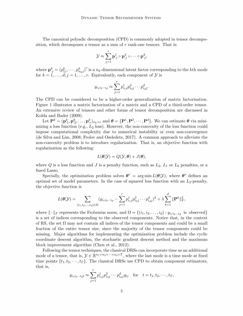
Figure 1: Illustration of factorizations of a matrix and a third-order tensor. (a) factorization of a matrixinto r rank-1 matrices, (b) CPD of a third-order tensor into r rank-1 tensors.
4
Dynamic Tensor Recommender Systems
The canonical polyadic decomposition (CPD) is commonly adopted in tensor decompo-sition, which decomposes a tensor as a sum of r rank-one tensors. That is:
Y ≈r∑j=1
p1·j p2
·j · · · pd·j ,
where pk·j = (pk1j , · · · , pknkj)> is a nk-dimensional latent factor corresponding to the kth mode
for k = 1, . . . , d; j = 1, . . . , r. Equivalently, each component of Y is
yi1i2···id ≈r∑j=1
p1i1jp
2i2j · · · p
didj.
The CPD can be considered to be a higher-order generalization of matrix factorisation.Figure 1 illustrates a matrix factorization of a matrix and a CPD of a third-order tensor.An extensive review of tensors and other forms of tensor decomposition are discussed inKolda and Bader (2009).
Let Pk = (pk·1,pk·2, . . . ,p
k·r)nk×r and θ = P1,P2, · · · ,Pd. We can estimate θ via mini-
mizing a loss function (e.g., L2 loss). However, the non-convexity of the loss function couldimpose computational complexity due to numerical instability or even non-convergence(de Silva and Lim, 2008; Frolov and Oseledets, 2017). A common approach to alleviate thenon-convexity problem is to introduce regularization. That is, an objective function withregularization as the following:
L(θ|Y) = Q(Y,θ) + J(θ),
where Q is a loss function and J is a penalty function, such as L2, L1 or L0 penalties, or afused Lasso.
Specially, the optimization problem solves θ∗ = arg minL(θ|Y), where θ∗ defines anoptimal set of model parameters. In the case of squared loss function with an L2-penalty,the objective function is
L(θ|Y) =∑
(i1,i2,...,id)∈Ω
(yi1i2···id −r∑j=1
p1i1jp
2i2j · · · p
didj
)2 + λd∑
k=1
‖Pk‖2F ,
where ‖ · ‖F represents the Frobenius norm, and Ω = (i1, i2, . . . , id) : yi1i2...id is observedis a set of indices corresponding to the observed components. Notice that, in the contextof RS, the set Ω may not contain all indices of the tensor components and could be a smallfraction of the entire tensor size, since the majority of the tensor components could bemissing. Major algorithms for implementing the optimization problem include the cycliccoordinate descent algorithm, the stochastic gradient descent method and the maximumblock improvement algorithm (Chen et al., 2012).
Following the tensor techniques, the classical DRSs can incorporate time as an additionalmode of a tensor, that is, Y ∈ Rn1×n2×···×nd×T , where the last mode is a time mode at fixedtime points t1, t2, · · · , tT . The classical DRSs use CPD to obtain component estimators,that is,
yi1i2···idt ≈r∑j=1
p1i1jp
2i2j · · · p
didjqtj for t = t1, t2, · · · , tT ,
5
Zhang, Bi, Tang and Qu
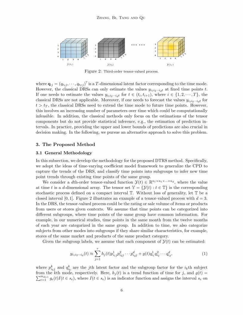
Figure 2: Third-order tensor-valued process.
where q·j = (qt1j , · · · , qtT j)> is a T -dimensional latent factor corresponding to the time mode.However, the classical DRSs can only estimate the values yi1i2···idt at fixed time points t.If one needs to estimate the values yi1i2···idt for t ∈ (ti, ti+1), where i ∈ 1, 2, · · · , T, theclassical DRSs are not applicable. Moreover, if one needs to forecast the values yi1i2···idt fort > tT , the classical DRSs need to extend the time mode to future time points. However,this involves an increasing number of parameters over time which could be computationallyinfeasible. In addition, the classical methods only focus on the estimations of the tensorcomponents but do not provide statistical inference, e.g., the estimation of prediction in-tervals. In practice, providing the upper and lower bounds of predictions are also crucial indecision making. In the following, we pursue an alternative approach to solve this problem.
3. The Proposed Method
3.1 General Methodology
In this subsection, we develop the methodology for the proposed DTRS method. Specifically,we adopt the ideas of time-varying coefficient model framework to generalize the CPD tocapture the trends of the DRS, and classify time points into subgroups to infer new timepoint trends through existing time points of the same group.
We consider a dth-order tensor-valued function Y(t) ∈ Rn1×n1×...×nd , where the valueat time t is a d-dimensional array. The tensor set Y = Y(t) : t ∈ T is the correspondingstochastic process defined on a compact interval T. Without loss of generality, let T be aclosed interval [0, 1]. Figure 2 illustrates an example of a tensor-valued process with d = 3.In the DRS, the tensor-valued process could be the rating or sale volume of items or productsfrom users or stores given contexts. We assume that time points can be categorized intodifferent subgroups, where time points of the same group have common information. Forexample, in our numerical studies, time points in the same month from the twelve monthsof each year are categorized in the same group. In addition to time, we also categorizesubjects from other modes into subgroups if they share similar characteristics, for example,stores of the same market and products of the same product category.
Given the subgroup labels, we assume that each component of Y(t) can be estimated:
yi1i2···id(t) ≈r∑j=1
hj(t)p1i1jp
2i2j · · · p
didj
+ g(t)q1i1q
2i2 · · · q
did, (1)
where pkikj and qkik are the jth latent factor and the subgroup factor for the ikth subjectfrom the kth mode, respectively. Here, hj(t) is a trend function of time for j, and g(t) =∑md+1
e=1 ge(t)I(t ∈ se), where I(t ∈ se) is an indicator function and assigns the interval se on
6
Dynamic Tensor Recommender Systems
the eth subgroup, ge(t) is a trend function corresponding to the eth subgroup, and md+1 isthe number of subgroups for time. We have qkik = qki′k
= qk(ek) if the ikth and i′kth subjects
are from the ekth subgroup (ek = 1, 2, . . . ,mk), where qk(ek) is the subgroup factor associatedwith the ekth subgroup, and mk is the number of subgroups for the kth mode. We denotethe set of observed time points for the component yi1i2···id(t) by Ti1i2...id , and the numberof components of this set by |Ti1i2...id |. Let yi1i2...id = yi1i2···id(t)t∈Ti1i2...id
. We assume
that the covariance matrix is cov(yi1i2...id) = Σ0i1i2...id
, typically not an identity matrix dueto the intra-cluster correlation arising from repeated observed data.
Equation (1) adopts the idea of varying-coefficient models to create a CPD for ten-sor data. Varying-coefficient models are a useful tool to explore dynamic patterns, andhave been applied to modeling and predicting longitudinal, functional and time series data(Huang and Shen, 2004; Fan and Zhang, 2008). Based on the varying-coefficient models,through the equations (1), we can obtain estimators of the component of tensor-value func-tion at any time points in a continuous time interval (e.g., t ∈ (a, b)) instead of at fixedtime points as in the DRS approaches (e.g., Xiong et al., 2010; Bi et al., 2018). The firstpart of equation (1) is an individual-level factor model which takes into account the hetero-geneity of subjects and trend of time, and the time-varying coefficients hj(t) (j = 1, . . . , r)reflect the dynamic features. The second part of equation (1) is a subgroup-level factormodel to capture common features from the same subgroups, where the subgroup factorscan accommodate new subjects from any mode at future time points, and the g(t) allowstime variables to follow a subgroup function of time such that we can predict future timepoints via borrowing information from existing time points of the same group.
To capture these trend functions, we adopt the polynomial splines to approximate hj(t)and ge(t). Let νjiaNi=1 be interior knots within T, and Υj be a partition of T with aN knots,that is Υj = 0 = νj0 < νj1 < · · · < νjaN < νjaN+1 = 1 for j = 1, 2, . . . , d. The polynomialsplines of an order κ+1 are functions with κ-degree of polynomials on intervals [νji−1, νji) fori = 1, 2, . . . , aN and [νjaN , νjaN+1], and have κ− 1 continuous derivatives globally. Denotea spline bases vector of the space of such spline functions as Bj(t) = (Bj1(t), . . . , BjM (t))>,where M = aN + κ + 1 as the number of spline bases. The function hj(t) (j = 1, 2, . . . , d)can be approximated by
hj(t) =∑M
i=1 αjiBji(t) = α>jBj(t),
where αj = (αj1, αj2, . . . , αjM )> is a coefficient vector. Spline functions can be B-splineor truncated polynomial functions. For example, for the truncated polynomial function,Bj(t) = (1, t, . . . , tκ, (t − νj1)κ+, . . . , (t − νjaN )κ+)>, and the (t − ν)+ is t − ν if t > ν and 0otherwise.
Similarly, let ωeiaNi=1 be interior knots within T, Γe = 0 = ωe0 < ωe1 < · · · <ωeaN < ωeaN+1 = 1, and Ae(t) = (Ae1(t), . . . , AeM (t))> be a vector of spline bases fore = 1, 2, . . . ,md+1. The ge(t) can be approximated by
ge(t) =M∑i=1
βeiAei(t) = β>eAe(t),
7
Zhang, Bi, Tang and Qu
where βe = (βe1, βe2, . . . , βeM )>. Based on equation (1), the prediction can be obtain asfollows
yi1i2···id(t) =r∑j=1
hj(t)p1i1jp
2i2j · · · p
didj
+ g(t)q1i1q
2i2 · · · q
did, (2)
where g(t) =∑md+1
e=1 ge(t)I(t ∈ se). The equation (2) can capture trends of the DRS suffi-ciently through the polynomial spline approximations of time-varying coefficient functions.In addition, since the spline approximation is computationally fast (Xue and Yang, 2006),the equation (2) can achieve the spline estimates of the coefficients efficiently, and this isespecially advantageous in estimating high-dimensional parameters in RS. In contrast tothese approaches like Xiong et al. (2010) and Bi et al. (2018), equation (2) can achieveforecasting at any future time points without requiring an increasing number of parametersover time. Note that the proposed method does not require the same number of knots andthe same degree polynomial for either trend functions. In order to reduce the computationalcost, we fixed the same numbers of knots and the same degree polynomial. We can alsoadopt different number of knots or different degree polynomial for different trend functionsg(t) and hj(t) respectively, or apply existing methods (Van Loock et al., 2011; Yuan et al.,2013; Dung and Tjahjowidodo, 2017) to identify the number of knots.
Due to the intra-cluster correlation, it is important to incorporate intra-cluster correla-tion into RS. However, in practice, the covariance matrix Σ0
i1i2...idis often unknown. We
adopt an invertible working covariance matrix, denoted as Σi1i2...id , to take into account theintra-cluster correlation. Let P = (P1>, · · · ,Pd>), q = (q(1)>, · · · ,q(d)>)>, α = (α>1, . . . ,α
>r)>,
β = (β>1, . . . ,β>md+1
)>, and γ = (α>,β>)>, where Pk = (pk·1, . . . ,pk·r), pk·j = (pk1j , · · · , pknkj
)>,
q(k) = (qk(1), . . . , qk(mk))
>, and k = 1, . . . , d. Define θ = P,q,γ as parameters of interest.Considering the intra-cluster correlation and non-convexity problem, we define the followingweighted penalized objective function:
L(θ|Y) =∑
(i1,i2,···,id)∈Ω
(yi1i2...id−yi1i2...id)>Σ−1i1i2...id
(yi1i2...id−yi1i2...id)+λ(‖P‖2F+‖q‖22+‖γ‖22),
(3)where λ is the penalized parameter, Ω = (i1, i2, . . . , id) : yi1i2···id(t) is observed at some t,‖ · ‖2 is the Euclidean norm, and yi1i2...id = yi1i2···id(t)t∈Ti1i2...id
is a |Ti1i2...id | × 1 vector.
The matrix Σi1i2...id is an approximation of the true covariance Σ0i1i2...id
, and can be
modeled as Σi1i2...id = V1/2i1i2...id
Ri1i2...idV1/2i1i2...id
, where Vi1i2...id is a diagonal matrix ofthe marginal variance of yi1i2...id , and Ri1i2...id is a working correlation matrix for yi1i2...id .Some commonly used working correlation structures include independence, exchangeable,and first-order autoregressive process (AR-1), among others. Given a working correlationstructure, the working correlation matrix depends on fewer nuisance parameters whichcan be estimated by the residual-based moment method (Liang and Zeger, 1986). Theproposed method is robust to the misspecification of correlation structure as indicated byour numerical examples.
3.2 Parameter Estimation
In this subsection, we discuss parameter estimation by minimizing (3). Let pkik = (pkik1, · · · ,pkikr)
> and Ωkik
= (i1, . . . , ik, . . . , id) : yi1···ik···id(t) is observed at some t given ik be the
8
Dynamic Tensor Recommender Systems
set of indices with the fixed kth mode index ik, where the corresponding components areobserved at some time points. We assume that the number of observations for each timesubgroup se is larger or equal than 2 for e = 1, . . . ,md+1, and the number of observations foreach subgroup ek from the kth mode is larger or equal than 2 for ek = 1, . . . ,mk; k = 1, . . . , d.The partial derivatives of the objective function (3) have explicit forms with respect to theindividual factors, the subgroup factors and the spline coefficients, which makes it feasibleto apply the blockwise coordinate descent approach (BCD). That is, for ik = 1, . . . , nk andk = 1, . . . , d,
pkik = arg minpkik
∑Ωk
ik
(yi1···ik···id − yi1···ik···id)>Σ−1i1···ik···id(yi1···ik···id − yi1···ik···id) + λ‖pkik‖
22, (4)
q(k) = arg minq(k)
∑Ω
(yi1i2···id − yi1i2···id)>Σ−1i1i2···id(yi1i2···id − yi1i2···id) + λ‖q(k)‖22, (5)
α = arg minα
∑Ω
(yi1i2···id − yi1i2···id)>Σ−1i1i2···id(yi1i2···id − yi1i2···id) + λ‖α‖22, (6)
β = arg minβ
∑Ω
(yi1i2···id − yi1i2···id)>Σ−1i1i2···id(yi1i2···id − yi1i2···id) + λ‖β‖22. (7)
In fact, the estimation procedure of pkik in (4) is a ridge regression, and does not require
knowing pki′kfor i′k 6= ik. Thus, parallel computation is applicable to calculate pk1, . . . , p
knk−1
and pknkefficiently. The minimization of L(θ|Y) can be done cyclically through estimating
P, q, α and β. Notice that Ω = ∪nkik=1Ωk
ik, and it is possible that Ωk
ikis empty for certain ik’s,
that is, there is no observation on the subject ik. Under this circumstance, the individualfactor of the ik subject is assigned as pkik = 00, and the predicted values may degenerateto the subgroup-level factor model by utilizing information from members of the samesubgroup.
3.3 Implementation
In the following, we discuss several implementation issues. To solve the objective function(3), we incorporate the maximum block improvement (MBI) strategy (Chen et al., 2012)into the BCD algorithm cyclically as in Bi et al. (2018). The MBI has two advantagesover traditional cyclic BCD algorithms. First, it has a good algorithmic property whichguarantees convergence to a stationary point, whereas traditional BCDs may end up withcertain points where the criterion function ceases to decrease (Chen et al., 2012). Second,the MBI has the capability of choosing descending directions and hence has the possibilityto discover “shortcuts”, which may reduce the computational time significantly. Let θl bean estimator of θ at the lth iteration, θa be a subset of θ, θc be the complementary set ofθa, and θ
∗a be the attempted update of θa. The improvement of the θ
∗a is defined as
Jθ∗a= 1−
L(θ∗a, θ
c
l−1|Y)
L(θl−1|Y). (8)
We summarize the implementation of the specifical algorithm as follows.
9
Zhang, Bi, Tang and Qu
Algorithm Implementation Algorithm
1: (Initialization) Input all observed yi1i2···id(t)’s, the number of factors r, tuning parameterλ, initial value θ0 and a stopping criterion ε = 10−4.
2: (Individual factors update) At the lth iteration, estimate P1,P2, · · · ,Pd,α.
(i) For each Pk, solve (4) through parallel computing and obtain Pk∗. Then calculateJPk∗ through (8).
(ii) For α, solve (6) and obtain α∗. Then calculate Jα∗ through (8).
(iii) AssignPkl ← Pk∗, if J
Pk∗ = maxJP1∗ , JP2∗ , · · · , JPd∗ , Jα∗.
α(l) ← α∗, if Jα∗ = maxJP1∗ , JP2∗ , · · · , JPd∗ , Jα∗.
3: (Subgroup factors update) At the lth iteration, estimate q(1),q(2), · · · ,q(d),β.
(i) For every q(k), solve (5) and obtain q(k)∗. Then calculate Jq(k)∗ through (8).
(ii) For β, solve (7) and obtain β∗. Then calculate Jβ∗ through (8).
(iii) Assign
q(k)l ← q(k)∗, if Jq(k)∗ = maxJq(1)∗ , Jq(2)∗ , · · · , Jq(d)∗ , Jβ∗.β(l) ← β
∗, if Jβ∗ = maxJq(1)∗ , Jq(2)∗ , · · · , Jq(d)∗ , Jβ∗.
4: (Stopping Criterion) Stop if maxJP1∗ , JP2∗ , · · · , JPd∗ , Jα∗ , Jq(1)∗ , · · · , Jq(d)∗ , Jβ∗ < ε.
Set the final estimator θ = θl. Otherwise set l← l + 1 and go to step 2.
To select tuning parameter λ, we search the one from grid points minimizing the rootmean square error on the validation set, defined as [
∑(i1,...,id,t)∈Γyi1...id(t)−yi1...id(t)2/|Γ|]1/2,
where Γ is the set of indices and times of observed data. We choose the number of individuallatent factors r such that it is sufficiently large and leads to stable estimation. In general,the r is no smaller than the theoretical rank of the tensor in order to represent subjects’latent features sufficiently well, but not so large as to over-burden the computational cost.
An appropriate selection of the knot sequence is important to efficiently implementthe proposed method. In practice, knot locations are usually chosen to be equally-spacedover the range of data or placed at evenly-spaced quantiles of data. Since there are high-dimensional factor parameters, for simplicity we set the number of knots to be the integerpart of N1/(2κ+3), where N = |Ω| and κ is the degree of polynomials. One can also chooseother methods to select the number of knots such as the AIC or BIC procedures (Xueand Yang, 2006). The degree of polynomials κ is commonly chosen as 1, 2, or 3. In ournumerical study, we set κ = 2 and adopt truncated polynomial bases. One can also usedifferent degrees and spline bases for different time-varying coefficients.
Another important issue is in selection of contextual variables as tensor modes. Inpractice, the chosen number of contexts is often pre-specified based on domain knowledge.A contextual variable can be considered an additional tensor mode of a higher-order tensor ifusers’ and items’ behaviors are distinctive under different values of the contextual variable.
10
Dynamic Tensor Recommender Systems
On the one hand, a higher-order tensor with more contextual variables allows higher-orderinteractions and hence provides more accurate estimation. On the other hand, a higher-order tensor entails more complex and intensive computation, and may lead to overfitting.It is not suggested to assign too many contextual variables as additional tensor modes, whichremains open to discussion regarding the number of contextual variables. In our numericalstudies, promotion strategies are incorporated as a contextual variable, since users’ anditems’ behaviors are distinctive under different promotion strategies. In general practice,however, we assume that the order of a tensor can be determined based on prior knowledge.
4. Theoretical Properties
In this section, we provide asymptotic properties for the proposed method and the estima-tion of prediction intervals. Specifically, we establish the convergence rate of the proposedtensor factorization and the asymptotic normality of the spline coefficient estimator. Fol-lowing asymptotic normality, we can also construct the estimation of the prediction intervalof the component. Note that identifiability is critical for tensor representation. We firstpresent the sufficient conditions to ensure identifiability of the proposed tensor modeling asfollows.
Proposition 1 If∑d
k=1Kk ≥ 2r + d+ 1 holds, minimizers of L(P,q,α,β|Y) in P, q, αand β given fixed spline bases are unique up to permutation almost surely, where Kk is theKruskal rank of (Pk,qk), and qk = (qk1 , q
k2 , · · · , qknk
)>.
Proposition 1 shows that the proposed tensor modeling is identifiable up to permutationalmost surely. To address permutation indeterminacy, we could align the factors accordingto a descending order of the first row of mode-1 factor matrix P1, that is, p1
11 ≥ p112 ≥ · · · ≥
p11r, following the method in Zhang et al. (2014). The rearrangement can be implemented
during or after the proposed algorithm, since it does not affect the estimation procedure.In the rest of Section 4, we assume that the parameters are identifiable.
Let ui1i2...id = (p1i11p
2i21 · · · pdid1), (p1
i12p2i22, · · · pdid2), · · · , (p1
i1rp2i2r· · · pdidr), (q
1i1q2i2· · · qdid)>,
U ∈ Rn1×...×nd×(r+1) consist of ui1i2...id , f(t) = h1(t), h2(t), . . . , hr(t), g(t)>, Fi1i2...id ∈R|Ti1i2...id
|×(r+1) be the matrix consisting of f(t) for all t ∈ Ti1i2···id . Considering random er-rors based on the equation (1), we denote yi1i2···id(t) as yi1i2···id(t) = f(t)>ui1i2...id +εi1i2...id(t)for t ∈ Ti1i2···id , where εi1i2...id(t) is a random error with mean zero and finite variance.Let εi1i2...id = εi1i2...id(t)t∈Ti1i2...id
be a |Ti1i2...id | × 1 vector. We have cov(εi1i2...id) =
cov(yi1i2...id) = Σ0i1i2...id
. Thus, the corresponding vector form is
yi1i2...id = Fi1i2...idui1i2...id + εi1i2...id ,
Let J(U) be a non-negative penalty function of U . The overall criterion given hj(·) and g(·)is redefined as
L(U|Y) =∑
(i1,i2,···,id)∈Ω
(yi1i2...id−Fi1i2...idui1i2...id)>Σ−1i1i2...id
(yi1i2...id−Fi1i2...idui1i2...id)+λJ(U)
(9)for U ∈ S, where S is the parameter space for U .
11
Zhang, Bi, Tang and Qu
Based on the proposed method, yi1i2...id can be rewritten as yi1i2...id = Wi1i2...idγ, whereWi1i2...id = (Xi1i2...id1, · · · ,Xi1i2...idr,Zi1i2...id1, · · · ,Zi1i2...idmd+1
), Xi1i2...idj = ui1i2...idjBi1i2...idj ,
Zi1i2...ide = ui1i2...id(r+1)Ai1i2...ide, in which Bi1i2...idj = Bj(t)>t∈Ti1i2...id
∈ R|Ti1i2...id|×M ,
and Ai1i2...ide = I(t ∈ se)Ae(t)>t∈Ti1i2...id
∈ R|Ti1i2...id|×M for j = 1, 2, . . . , r, e = 1, 2, . . . ,
md+1. By the approximation theory (de Boor, 2001), there exists a constant C > 0, thespline functions hj(t) = α>0jBj(t) and ge(t) = β>0eAe(t) such that supt∈T |hj(t) − hj(t)| ≤Ca−ξN and supt∈T |ge(t) − ge(t)| ≤ Ca−ξN for any j = 1, . . . , r, e = 1, . . . ,md+1. Denoteγ0 = (α>0,β
>0)>, and let N = |Ω| be the number of components of the set Ω, λmin· and
λmax· be the smallest and largest eigenvalues of any symmetric matrix, respectively. Werequire the following regularity conditions to establish the asymptotic properties.
(C1) The functions hj(·) and ge(·) are ξth-order continuously differential for some ξ ≥ 2, allj = 1, . . . , d, and e = 1, . . . ,md+1. The density function of design points t is absolutelycontinuous and bounded away from zero and infinity on a compact support T.
(C2) The knots sequences Υj and Γe are quasi-uniform for j = 1, . . . , d and e = 1, . . . ,md+1;that is, there exists a constant c > 0, such that
maxj=1,...,d
maxi=0,...,aN (νji+1 − νji)mini=0,...,aN (νji+1 − νji)
≤ c, and maxe=1,...,md+1
maxi=0,...,aN (ωei+1 − ωei)mini=0,...,aN (ωei+1 − ωei)
≤ c.
(C3) There exist positive constants σ21 and σ2
2 such that the covariance matrix Σ0i1i2...id
of
random error εi1...id satisfies that σ21 ≤ λminΣ0
i1i2...id ≤ λmaxΣ0
i1i2...id ≤ σ2
2.
(C4) There exist some positive constants c1 and c2 such that c1 ≤ λminΣ−1i1i2...id
Σ0i1i2...id
≤λmaxΣ−1
i1i2...idΣ0i1i2...id
≤ c2.
(C5) Tmax = max(i1,···,id)∈Ω|Ti1···id | = op(Nτ ), Tmin = min(i1,···,id)∈Ω|Ti1···id | = op(N
υ)for 0 ≤ τ/2 < υ ≤ τ < 1, and λ = op(1).
Conditions (C1)-(C3) are standard in the polynomial spline framework. Similar con-ditions are also presented in Huang (2003) and Claeskens et al. (2009). In particular,condition (C1) imposes a smoothness condition of trend functions and a mild condition ontime density, and guarantees that the observation time points are randomly scattered. Con-dition (C2) indicates that the adjacent distances among the knot sequence are comparable.Condition (C3) implies that the eigenvalues of random errors are bounded. Condition (C4)implies that the difference between the working covariance and true covariance matrices isbounded. Condition (C5) implies that the number of the observed time points grows as thenumber of the observed components of the tensor increases, to ensure the convergence ofthe proposed tensor factorization. The following theorem establishes the convergence ratefor the proposed tensor factorization.
Theorem 2 Under conditions (C1)-(C5), if the penalty function J(U) has bounded firstand second derivatives at true parameter U0, as N → ∞, on a δ-ball centered at U0 forsome δ > 0, there exists a minimizer U of (9) such that∑
(i1,i2,···,id)∈Ω
‖Fi1i2···id(ui1i2···id − u0i1i2···id)‖22/N = Op(N−1+2(τ−υ)).
12
Dynamic Tensor Recommender Systems
Theorem 2 provides the convergence rate of the proposed method given trend functions.When τ = υ, that is, Tmax and Tmin have the same order, the convergence rate of theestimator U reaches the optimal rate N−1/2. Meanwhile, if the order of Tmax is
√N faster
than that of Tmin, that is, τ − υ = 0.5, then U will not converge to the true U0. Thisimplies that to guarantee consistency of the tensor factorization, one should collect sufficientobservations even for the least popular user-item-context combinations. In the followingtheorem, we establish the asymptotic property of the spline coefficient estimator.
Theorem 3 Under conditions (C1)-(C5), if limN→∞ aN log aN/N = 0 and limN→∞ a−ξN N τ
= 0, then for any vector c whose components are not all zero, the parametric estimator γby (6) and (7) satisfies
c>(γ − γ0)varc>(γ − γ0)−1/2 L→ N(0, 1),
where varc>(γ−γ0) = c>Ψ−1ΦΨ−1c = Op(aNN−1+τ−2υ), Ψ =
∑(i1,...,id)∈Ω W>
i1...idΣ−1i1...id·
Wi1...id, and Φ =∑
(i1,...,id)∈Ω W>i1...id
Σ−1i1...id
Σ0i1...id
Σ−1i1...id
Wi1...id.
Theorem 3 establishes the asymptotic normality of the spline coefficient estimator. Theconvergence rate of the spline coefficient estimator is Op(aNN
−1+τ−2υ). If Tmax and Tmin
have the same order, varc>(γ − γ0) = Op(aN/N1+υ), and similar results can be found
in Huang et al. (2004). The asymptotic variance in Theorem 3 depends on the workingcovariance matrix and the true covariance matrix. When the working covariance matricesare equal to the true covariance matrices, the asymptotic variance of the proposed estimatorreaches the minimum in the sense of Lower order and the proposed estimator is asymptoticefficient.
More importantly, the result of Theorem 3 is the key foundation for constructing predic-tion intervals. First, we derive the standard error for the spline parametric estimates given afixed λ using the sandwich covariance formula Cov(γ) = (Ψ+λI)−1Φ(Ψ+λI)−1, where Ψ =∑
(i1,i2,...,id)∈Ω W>i1i2...id
Σ−1i1i2...id
Wi1i2...id , Φ =∑
(i1,i2,...,id)∈ΩW>i1i2...id
Σ−1i1i2...id
(yi1i2...id −Wi1i2...id γ)⊗2, ⊗ operation is the vector operation a⊗2 = aa>, and I is an identity ma-
trix. Since yi1i2...id(t) = w>i1i2...idtγ, and wi1i2...idt is the tth column of estimator W>i1i2...id
,a 100(1− σ)% prediction interval (Chatfield, 1993) of yi1i2...id(t) is
yi1i2...id(t)± φσ/2√
varei1i2...id(t), (10)
where φσ/2 is the 100(1 − σ)th percentile of the standard normal distribution, and thevarei1i2...id(t) is the variance of the prediction error and can be estimated as:
varei1i2...id(t) = w>i1i2...idtCov(γ)wi1i2...idt + varεi1i2...id(t). (11)
The first term in equation (11) is due to estimation error, and the second term can beestimated by the mean squared error on training data.
13
Zhang, Bi, Tang and Qu
5. Simulation Studies
In this section, we perform simulation studies to compare the proposed method (DTRS) withcompeting methods, including Bayesian probabilistic tensor factorization (BPTF, Xionget al., 2010) and the recommendation engine of multilayers (REM, Bi et al., 2018). Weassess forecasting performance via examining the root mean square error (RMSE) andthe mean absolute error (MAE), where the RMSE is defined as [
∑(i1,...,id,t)∈Γyi1...id(t) −
yi1...id(t)2/|Γ|]1/2, the MAE is defined as∑
(i1,...,id,t)∈Γ |yi1...id(t) − yi1...id(t)|/|Γ|, and Γ isthe set of indices and time of observed data. Moreover, we evaluate the coverage probabilityof the prediction interval estimated by the proposed method with 95% nominal coverageprobability (PICP) .
5.1 Simple Tensor Function
In the simulation, we consider a third-order tensor function of time with user, context anditem modes. We set the numbers of users, contexts and items to n1 = 100, n2 = 9, andn3 = 100, respectively. We assume that users, contexts, items and time points are fromm1 = 10, m2 = 3, m3 = 10 and m4 = 4 subgroups, respectively. Users, contexts, itemsand time points are evenly assigned to each subgroup. The number of latent factors isset as r = 3. We generate tensor functions at time points t ∼ U(0, 1) by generating itscomponents as yi1i2i3(t) =
∑rj=1 hj(t)p
1i1jp2i2jp3i3j
+g(t)q1i1q2i2q3i3
+εi1i2i3(t) for ik = 1, . . . , nk,
k = 1, 2, 3, where the latent factors pkik ∼ N(0, Ir), trend functions h1(t) = sin(0.3πt),h2(t) = 8t(1− t)− 1 and h3(t) = cos(0.2πt) + 1. To distinguish different subgroups, we setthe subgroup factors as a simple sequence, where q1
(e1) = −1+0.4e1, q2(e2) = −1.2+0.6e2 and
q3(e3) = −0.4+0.2e3 for ek = 1, . . . ,mk and k = 1, 2, 3. The function g(t) =
∑m4e=1 ge(t)I(t ∈
se), where g1(t) = 2t − 1, g2(t) = 8(t − 0.5)3, g3(t) = sin(0.1πt) + cos(πt), and g4(t) =−5 exp(t)+10. The error εi1i2i3 = (εi1i2i3(t1), . . . , εi1i2i3(tT ))> follows a multivariate normaldistribution with mean 0 and a common marginal variance 1, and the correlation structureis either independence or AR-1 with correlation ρ = 0.85.
In each simulation, we consider the number of time points as T = T1 + T2, where thetensor data in the first T1 = 12 time points are set as the training data, and the tensordata in the last T2 time points are used as the testing data. For evaluating the forecastingperformance at future time points, we consider T2 = 8 or 12. Considering the missingcase, we generate n1n2n3T (1 − πm) components out of the tensor functions, where πm isthe missing percentage and set as 80%. Furthermore, we use πcs = 30% to represent theproportion of new items in the testing data unavailable from the training set. To illustratethe effect of incorporating intra-cluster correlation on estimation efficiency, we compare theestimation efficiency of the proposed methods using different working correlation structures:independent or AR-1, denoted as DTRSin and DTRSar, respectively.
According to Xiong et al. (2010) and Bi et al. (2018), BPTF and REM methods modelfourth-order tensor with user, context, item and time modes. For all methods, we assumethat the subgroup structure and the number of latent factors are known. For REM and theproposed methods, the tuning parameter λ is pre-selected from grid points ranging from 0to 20. The validation set is the data from the last four time points of the training set. ForBPTF, we keep the remaining parameters by their default choices and obtain a forecast
14
Dynamic Tensor Recommender Systems
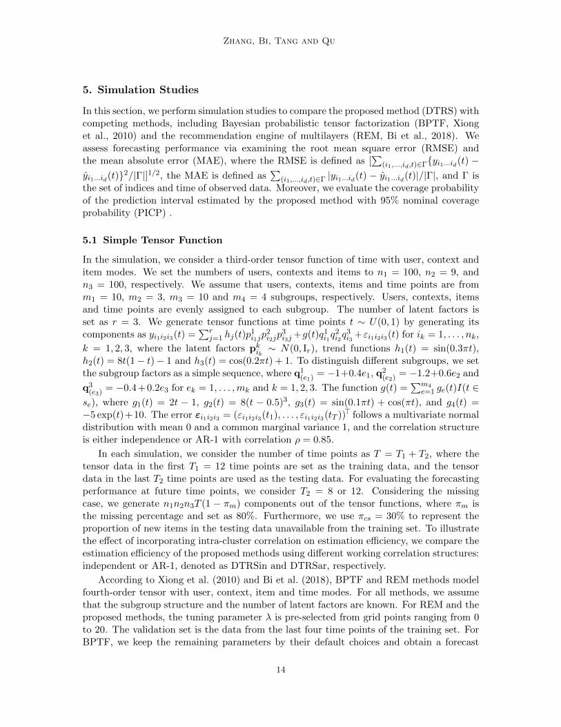
Table 1: Average RMSE and MAE of all approaches. The PICP is the average coverageprobability of the 95% prediction interval. The RMSE, MAE and PICP are pro-vided with standard error based on 100 simulations in each parenthesis.
True structure: Independent AR
Method T2 = 8 T2 = 12 T2 = 8 T2 = 12
DTRSin RMSE 1.570(0.196) 1.660(0.389) 1.597(0.192) 1.707(0.524)MAE 1.092(0.091) 1.132(0.160) 1.115(0.091) 1.160(0.208)PICP 0.949(0.015) 0.953(0.017) 0.946(0.017) 0.952(0.018)
DTRSar RMSE 1.625(0.244) 1.696(0.286) 1.576(0.190) 1.632(0.200)MAE 1.133(0.118) 1.170(0.159) 1.099(0.085) 1.130(0.102)PICP 0.943(0.019) 0.947(0.021) 0.947(0.015) 0.949(0.018)
REM RMSE 2.502(0.322) 2.494(0.307) 2.498(0.304) 2.494(0.305)MAE 1.654(0.178) 1.640(0.170) 1.650(0.166) 1.643(0.172)PICP – – – –
BPTFbayes RMSE 2.675(0.742) 2.930(0.965) 2.724(0.863) 3.181(1.148)MAE 1.810(0.427) 1.958(0.547) 1.826(0.495) 2.104(0.654)PICP – – – –
BPTFbasic RMSE 2.142(0.221) 2.145(0.211) 2.136(0.222) 2.144(0.206)MAE 1.446(0.116) 1.454(0.115) 1.441(0.117) 1.453(0.111)PICP – – – –
BPTFdouble RMSE 2.388(0.319) 2.665(0.356) 2.405(0.319) 2.642(0.380)MAE 1.598(0.190) 1.774(0.217) 1.611(0.191) 1.755(0.232)PICP – – – –
via sampling the factor matrix of time from the time posterior distribution, denoted asBPTFbayes. Following the forecasting technique of Araujo et al. (2019), we also considerBPTF incorporating basic exponential smoothing (Holt’s method, Holt, 2004) and doubleexponential smoothing (Holt-Winters method, Holt, 2004; Winters, 1960). That is, we firstuse BPTF to estimate the factor matrices of user, item, context and time in the trainingdata, and then forecast the factor matrix of time at given time points of the testing datavia basic exponential smoothing or double exponential smoothing, denoted as BPTFbasic
and BPTFdouble, respectively. All methods are replicated by 100 simulation runs.
Table 1 provides the estimation results of all methods. We observe that the proposedmethod has better performance when the working correlation structure is the same as thetrue correlation structure. When the true correlation structure is independence, the DTRSinhas smaller RMSE and MAE than the DTRSar, with more than 2.17% improvement. Sim-ilarly, when the true correlation structure is AR-1, the DTRSar outperforms the DTRSin.Moreover, the PICPs of the DTRS method are close to 0.95, which implies that the pro-posed method provides accurate prediction intervals, whereas the competing methods arenot able to provide such prediction intervals. For the performance of forecasting, we observethat the DTRSin and DTRSar outperform other methods across all settings. Specifically,both DTRS methods improve the RMSE and MAE of the REM by more than 40%, and
15
Zhang, Bi, Tang and Qu
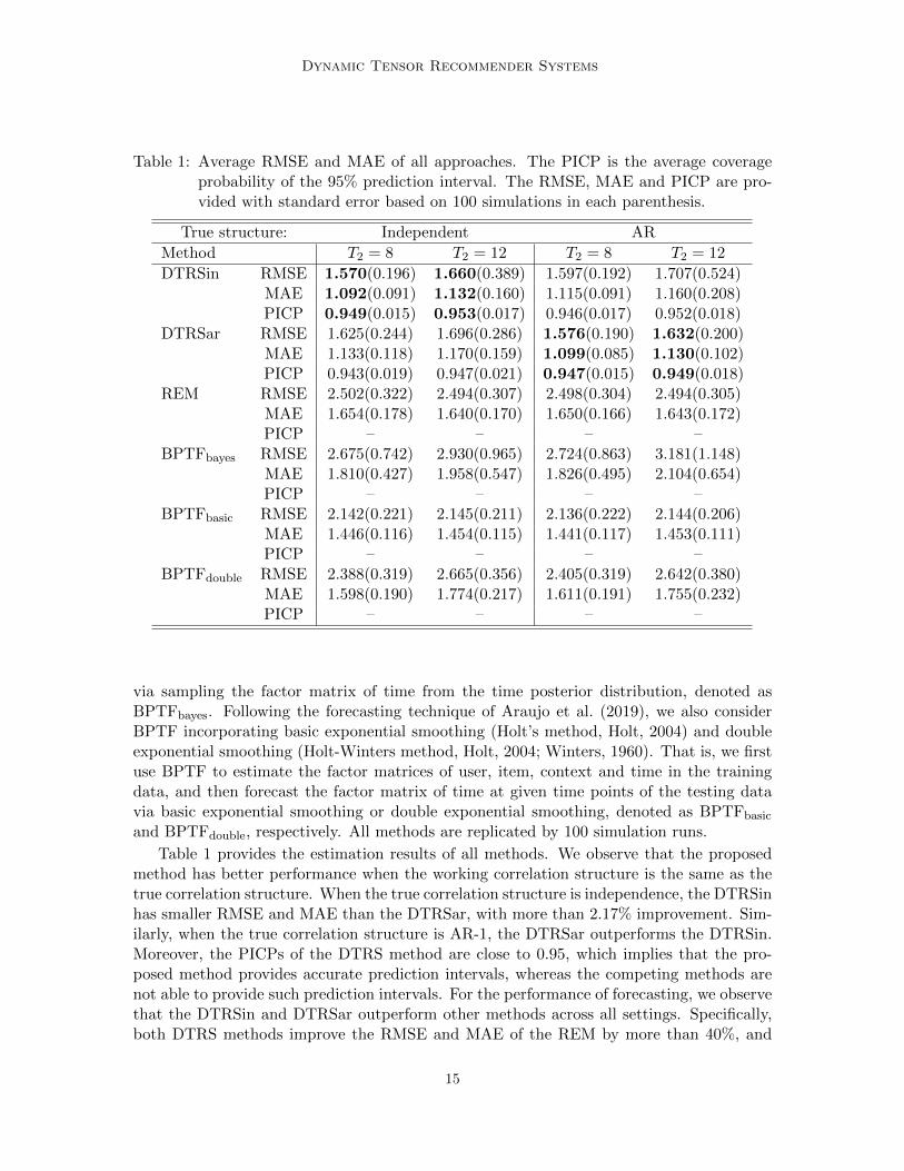
Figure 3: Box plots of the MAE for forecasting values with 8 and 12 time points and the true independentcorrelation.
those of the BPTFbayes, BPTFbasic and BPTFdouble by more than 60%, 24%, and 41%,respectively. In this setting, the BPTFbasic performs better than the BPTFdouble. This isprobably because the basic exponential smoothing method is more applicable in forecastingtime series with no clear trend or seasonal pattern, whereas the double exponential smooth-ing method performs better when a trend is present (Holt, 2004). Although the BPTFbasic
and BPTFdouble perform better than the BPTFbayes, the proposed method is still able tobeat the best of the BPTF variations. This indicates that the proposed method providesmore accurate forecasting compared to other methods.
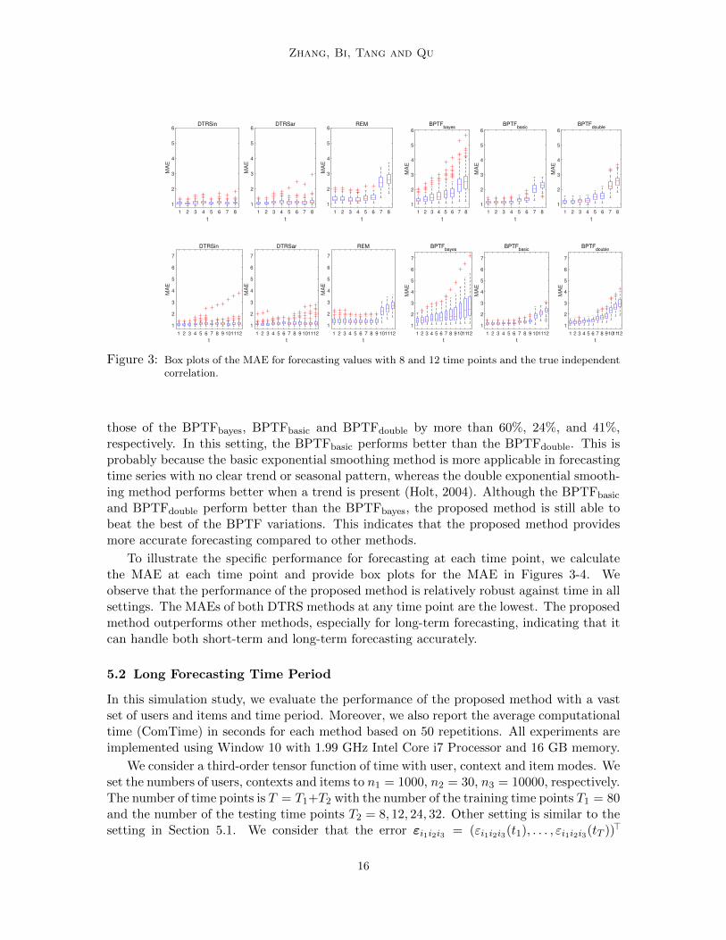
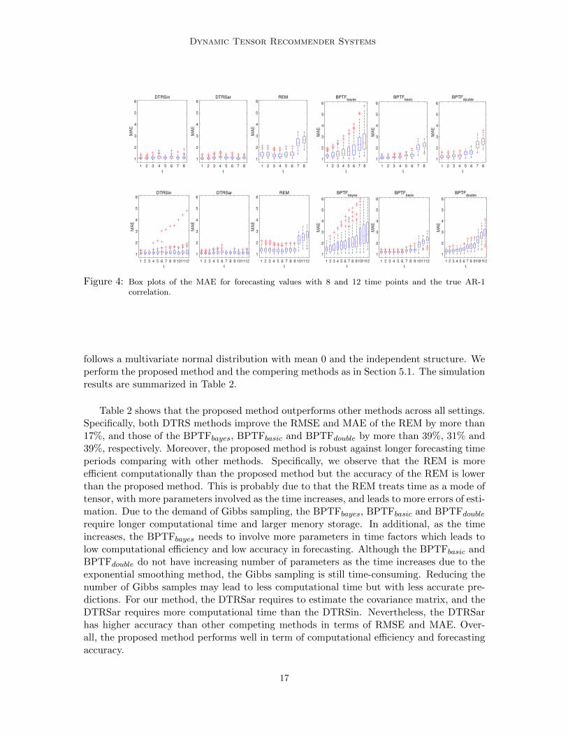
To illustrate the specific performance for forecasting at each time point, we calculatethe MAE at each time point and provide box plots for the MAE in Figures 3-4. Weobserve that the performance of the proposed method is relatively robust against time in allsettings. The MAEs of both DTRS methods at any time point are the lowest. The proposedmethod outperforms other methods, especially for long-term forecasting, indicating that itcan handle both short-term and long-term forecasting accurately.
5.2 Long Forecasting Time Period
In this simulation study, we evaluate the performance of the proposed method with a vastset of users and items and time period. Moreover, we also report the average computationaltime (ComTime) in seconds for each method based on 50 repetitions. All experiments areimplemented using Window 10 with 1.99 GHz Intel Core i7 Processor and 16 GB memory.
We consider a third-order tensor function of time with user, context and item modes. Weset the numbers of users, contexts and items to n1 = 1000, n2 = 30, n3 = 10000, respectively.The number of time points is T = T1+T2 with the number of the training time points T1 = 80and the number of the testing time points T2 = 8, 12, 24, 32. Other setting is similar to thesetting in Section 5.1. We consider that the error εi1i2i3 = (εi1i2i3(t1), . . . , εi1i2i3(tT ))>
16
Dynamic Tensor Recommender Systems
Figure 4: Box plots of the MAE for forecasting values with 8 and 12 time points and the true AR-1correlation.
follows a multivariate normal distribution with mean 0 and the independent structure. Weperform the proposed method and the compering methods as in Section 5.1. The simulationresults are summarized in Table 2.
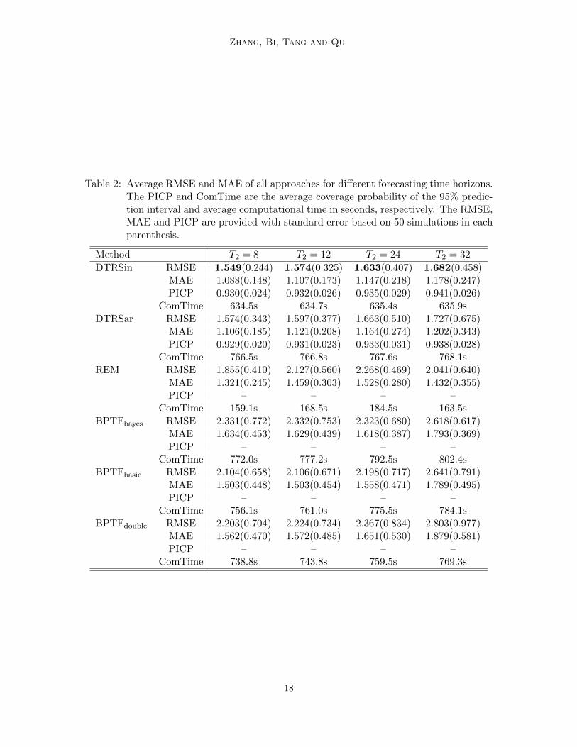
Table 2 shows that the proposed method outperforms other methods across all settings.Specifically, both DTRS methods improve the RMSE and MAE of the REM by more than17%, and those of the BPTFbayes, BPTFbasic and BPTFdouble by more than 39%, 31% and39%, respectively. Moreover, the proposed method is robust against longer forecasting timeperiods comparing with other methods. Specifically, we observe that the REM is moreefficient computationally than the proposed method but the accuracy of the REM is lowerthan the proposed method. This is probably due to that the REM treats time as a mode oftensor, with more parameters involved as the time increases, and leads to more errors of esti-mation. Due to the demand of Gibbs sampling, the BPTFbayes, BPTFbasic and BPTFdoublerequire longer computational time and larger menory storage. In additional, as the timeincreases, the BPTFbayes needs to involve more parameters in time factors which leads tolow computational efficiency and low accuracy in forecasting. Although the BPTFbasic andBPTFdouble do not have increasing number of parameters as the time increases due to theexponential smoothing method, the Gibbs sampling is still time-consuming. Reducing thenumber of Gibbs samples may lead to less computational time but with less accurate pre-dictions. For our method, the DTRSar requires to estimate the covariance matrix, and theDTRSar requires more computational time than the DTRSin. Nevertheless, the DTRSarhas higher accuracy than other competing methods in terms of RMSE and MAE. Over-all, the proposed method performs well in term of computational efficiency and forecastingaccuracy.
17
Zhang, Bi, Tang and Qu
Table 2: Average RMSE and MAE of all approaches for different forecasting time horizons.The PICP and ComTime are the average coverage probability of the 95% predic-tion interval and average computational time in seconds, respectively. The RMSE,MAE and PICP are provided with standard error based on 50 simulations in eachparenthesis.
Method T2 = 8 T2 = 12 T2 = 24 T2 = 32
DTRSin RMSE 1.549(0.244) 1.574(0.325) 1.633(0.407) 1.682(0.458)MAE 1.088(0.148) 1.107(0.173) 1.147(0.218) 1.178(0.247)PICP 0.930(0.024) 0.932(0.026) 0.935(0.029) 0.941(0.026)
ComTime 634.5s 634.7s 635.4s 635.9sDTRSar RMSE 1.574(0.343) 1.597(0.377) 1.663(0.510) 1.727(0.675)
MAE 1.106(0.185) 1.121(0.208) 1.164(0.274) 1.202(0.343)PICP 0.929(0.020) 0.931(0.023) 0.933(0.031) 0.938(0.028)
ComTime 766.5s 766.8s 767.6s 768.1sREM RMSE 1.855(0.410) 2.127(0.560) 2.268(0.469) 2.041(0.640)
MAE 1.321(0.245) 1.459(0.303) 1.528(0.280) 1.432(0.355)PICP – – – –
ComTime 159.1s 168.5s 184.5s 163.5sBPTFbayes RMSE 2.331(0.772) 2.332(0.753) 2.323(0.680) 2.618(0.617)
MAE 1.634(0.453) 1.629(0.439) 1.618(0.387) 1.793(0.369)PICP – – – –
ComTime 772.0s 777.2s 792.5s 802.4sBPTFbasic RMSE 2.104(0.658) 2.106(0.671) 2.198(0.717) 2.641(0.791)
MAE 1.503(0.448) 1.503(0.454) 1.558(0.471) 1.789(0.495)PICP – – – –
ComTime 756.1s 761.0s 775.5s 784.1sBPTFdouble RMSE 2.203(0.704) 2.224(0.734) 2.367(0.834) 2.803(0.977)
MAE 1.562(0.470) 1.572(0.485) 1.651(0.530) 1.879(0.581)PICP – – – –
ComTime 738.8s 743.8s 759.5s 769.3s
18
Dynamic Tensor Recommender Systems
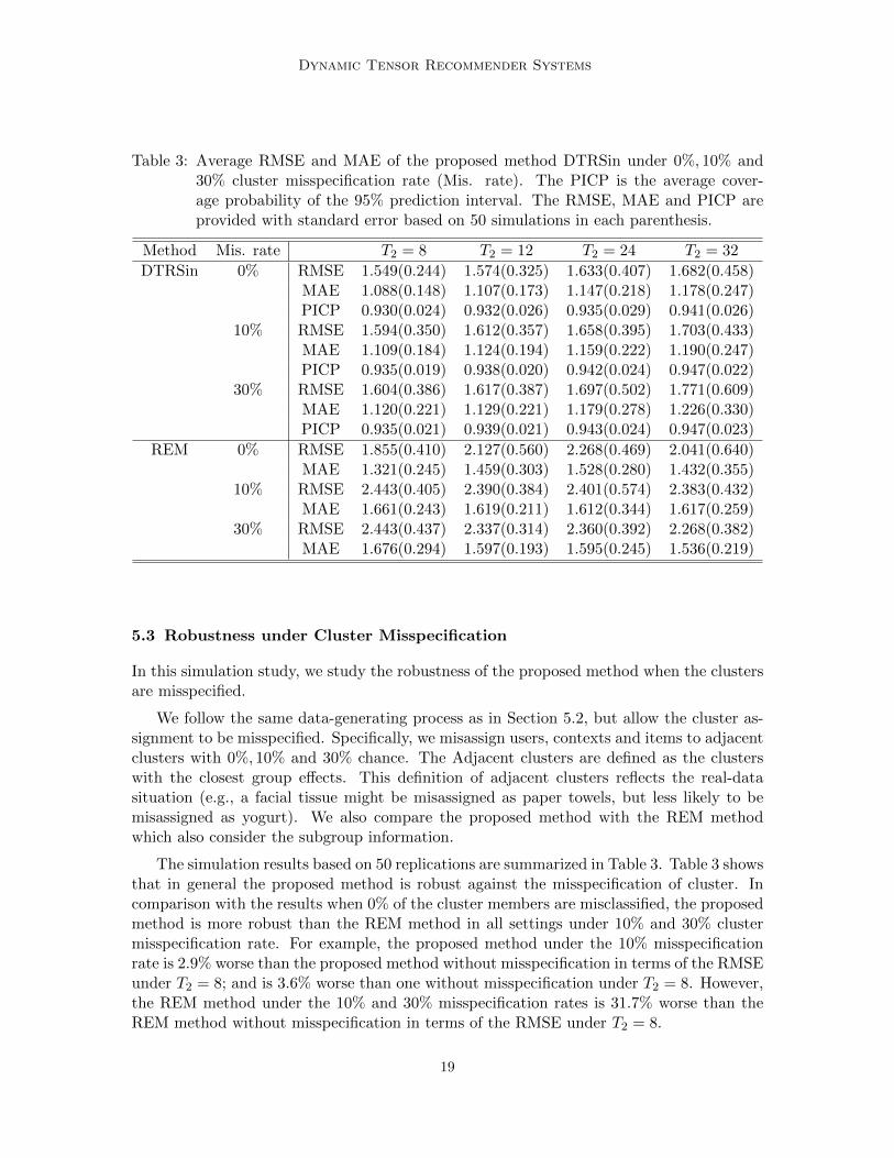
Table 3: Average RMSE and MAE of the proposed method DTRSin under 0%, 10% and30% cluster misspecification rate (Mis. rate). The PICP is the average cover-age probability of the 95% prediction interval. The RMSE, MAE and PICP areprovided with standard error based on 50 simulations in each parenthesis.
Method Mis. rate T2 = 8 T2 = 12 T2 = 24 T2 = 32
DTRSin 0% RMSE 1.549(0.244) 1.574(0.325) 1.633(0.407) 1.682(0.458)MAE 1.088(0.148) 1.107(0.173) 1.147(0.218) 1.178(0.247)PICP 0.930(0.024) 0.932(0.026) 0.935(0.029) 0.941(0.026)
10% RMSE 1.594(0.350) 1.612(0.357) 1.658(0.395) 1.703(0.433)MAE 1.109(0.184) 1.124(0.194) 1.159(0.222) 1.190(0.247)PICP 0.935(0.019) 0.938(0.020) 0.942(0.024) 0.947(0.022)
30% RMSE 1.604(0.386) 1.617(0.387) 1.697(0.502) 1.771(0.609)MAE 1.120(0.221) 1.129(0.221) 1.179(0.278) 1.226(0.330)PICP 0.935(0.021) 0.939(0.021) 0.943(0.024) 0.947(0.023)
REM 0% RMSE 1.855(0.410) 2.127(0.560) 2.268(0.469) 2.041(0.640)MAE 1.321(0.245) 1.459(0.303) 1.528(0.280) 1.432(0.355)
10% RMSE 2.443(0.405) 2.390(0.384) 2.401(0.574) 2.383(0.432)MAE 1.661(0.243) 1.619(0.211) 1.612(0.344) 1.617(0.259)
30% RMSE 2.443(0.437) 2.337(0.314) 2.360(0.392) 2.268(0.382)MAE 1.676(0.294) 1.597(0.193) 1.595(0.245) 1.536(0.219)
5.3 Robustness under Cluster Misspecification
In this simulation study, we study the robustness of the proposed method when the clustersare misspecified.
We follow the same data-generating process as in Section 5.2, but allow the cluster as-signment to be misspecified. Specifically, we misassign users, contexts and items to adjacentclusters with 0%, 10% and 30% chance. The Adjacent clusters are defined as the clusterswith the closest group effects. This definition of adjacent clusters reflects the real-datasituation (e.g., a facial tissue might be misassigned as paper towels, but less likely to bemisassigned as yogurt). We also compare the proposed method with the REM methodwhich also consider the subgroup information.
The simulation results based on 50 replications are summarized in Table 3. Table 3 showsthat in general the proposed method is robust against the misspecification of cluster. Incomparison with the results when 0% of the cluster members are misclassified, the proposedmethod is more robust than the REM method in all settings under 10% and 30% clustermisspecification rate. For example, the proposed method under the 10% misspecificationrate is 2.9% worse than the proposed method without misspecification in terms of the RMSEunder T2 = 8; and is 3.6% worse than one without misspecification under T2 = 8. However,the REM method under the 10% and 30% misspecification rates is 31.7% worse than theREM method without misspecification in terms of the RMSE under T2 = 8.
19
Zhang, Bi, Tang and Qu
6. Empirical Examples
6.1 IRI Marketing Data
In this section, we focus on sales data at drug stores from the IRI Marketing Data (Bron-nenberg et al., 2008) to illustrate the performance of the proposed method. The originalIRI data is an immense collection of consumer panel data and store sales at grocery stores,drug stores and mass-market stores over the years 2001-2011. The store sales data containweekly product sales volumes, pricing, and promotion data for all items from 31 productcategories sold in 50 U.S. markets. These markets are geographic units defined typically asan agglomeration of counties, usually covering a major metropolitan areas (e.g., Chicago,IL) but sometimes covering just part of a region (e.g., New England). A detailed descriptionof an early version of the data is available in Bronnenberg et al. (2008).
To illustrate the proposed method, we choose sales data at drug stores collected from2001 to 2011, where there are sales volume records, recorded times, promotion strate-gies, 43,631 product IDs, and 471 drug store IDs. These drug stores are from 50 marketsacross the United States. The products include items sold from these stores during the11-year period, and are from 31 product categories, including hot dogs, household cleaners,margarine/butter blends, mayonnaise, milk, coffee, cigarettes, photography supplies, pa-per towels, frozen pizza, toilet tissue, yogurt, beer/ale/alcoholic cider, blades, cold cereal,carbonated beverages, diapers, deodorant, facial tissue, frozen dinners/entrees, laundry de-tergent, peanut butter, razors, mustard and ketchup, sugar substitutes, spaghetti/Italiansauce, soup, shampoo, salty snacks, toothpaste, and toothbrush. Moreover, various adver-tising and promotions strategies are imposed on these products to attract consumers. Thepromotions strategies have 30 types which are combinations of 5 advertisement features, 3types of merchandise display, and an indicator on whether the product has a price reductionof more than 5%.
The goal of our study is to predict the future sales volumes of each product from eachstore given each promotion strategy based on historical sales data. Through this predictionprocedure, we are able to estimate future purchases, evaluate the influence of promotionstrategy for product sales, and potentially recommend the most profitable products tostore managers, so the company can make wiser decisions on marketing strategies andinventory planning. For the IRI marketing data, a personalized suggestion refers to therecommendation of potentially profitable products to store managers. Statistically thiscan be viewed as predicting future sales volumes of each product from each store basedon historical sales data. There are abundant literature on product recommender systemsincluding, but not limited to, Giering (2008), Xiong et al. (2010) and Yu et al. (2016). Inthese works, similar to the proposed IRI data analysis, recommendations of products tostores are also considered. For considering the trend of product sales, we aggregate theweekly data into monthly data according to the record time information so that the datacontain more than 79.2 million sales records for 132 months from the beginning of 2001to the end of 2011. For the proposed method, we classify stores, products, observed timepoints and promotion strategies into subgroups based on their markets, product categories,month of the year and whether a price reduction is applied, respectively.
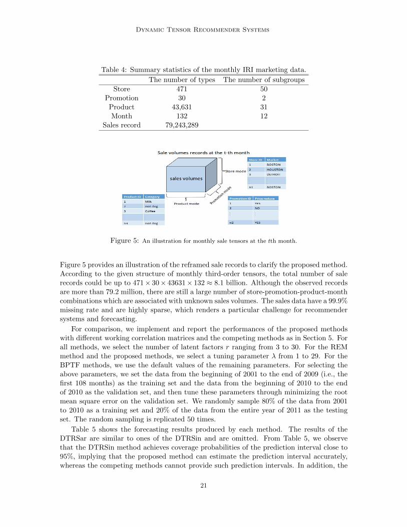
Table 4 shows the summary statistics of the data. According to the proposed method,the data can be reframed into monthly third-order tensors by store, product and promotion.
20
Dynamic Tensor Recommender Systems
Table 4: Summary statistics of the monthly IRI marketing data.
The number of types The number of subgroups
Store 471 50Promotion 30 2Product 43,631 31Month 132 12
Sales record 79,243,289
Figure 5: An illustration for monthly sale tensors at the tth month.
Figure 5 provides an illustration of the reframed sale records to clarify the proposed method.According to the given structure of monthly third-order tensors, the total number of salerecords could be up to 471× 30× 43631× 132 ≈ 8.1 billion. Although the observed recordsare more than 79.2 million, there are still a large number of store-promotion-product-monthcombinations which are associated with unknown sales volumes. The sales data have a 99.9%missing rate and are highly sparse, which renders a particular challenge for recommendersystems and forecasting.
For comparison, we implement and report the performances of the proposed methodswith different working correlation matrices and the competing methods as in Section 5. Forall methods, we select the number of latent factors r ranging from 3 to 30. For the REMmethod and the proposed methods, we select a tuning parameter λ from 1 to 29. For theBPTF methods, we use the default values of the remaining parameters. For selecting theabove parameters, we set the data from the beginning of 2001 to the end of 2009 (i.e., thefirst 108 months) as the training set and the data from the beginning of 2010 to the endof 2010 as the validation set, and then tune these parameters through minimizing the rootmean square error on the validation set. We randomly sample 80% of the data from 2001to 2010 as a training set and 20% of the data from the entire year of 2011 as the testingset. The random sampling is replicated 50 times.
Table 5 shows the forecasting results produced by each method. The results of theDTRSar are similar to ones of the DTRSin and are omitted. From Table 5, we observethat the DTRSin method achieves coverage probabilities of the prediction interval close to95%, implying that the proposed method can estimate the prediction interval accurately,whereas the competing methods cannot provide such prediction intervals. In addition, the
21
Zhang, Bi, Tang and Qu
Table 5: The RMSE and MAE of the forecasting sale volumes in 2011 from five methods.The PICP is the average coverage probability of the 95% prediction interval. TheRMSE, MAE and PICP are provided with standard error based on 50 experimentsin each parenthesis. The RRMSE and RMAE show the relative improvement ratiosof the DTRSin method over others in terms of the RMSE and MAE.
Method RMSE RRMSE MAE RMAE PICP
DTRSin 11.284(0.536) – 3.790(0.058) – 0.967(0.001)REM 13.425(1.458) 18.97% 4.072(0.261) 7.44% –BPTFbayes 15.792(1.746) 39.95% 4.276(0.171) 12.82% –BPTFbasic 12.736(0.385) 12.87% 3.838(0.058) 1.27% –BPTFdouble 12.732(0.388) 12.83% 3.835(0.057) 1.19% –
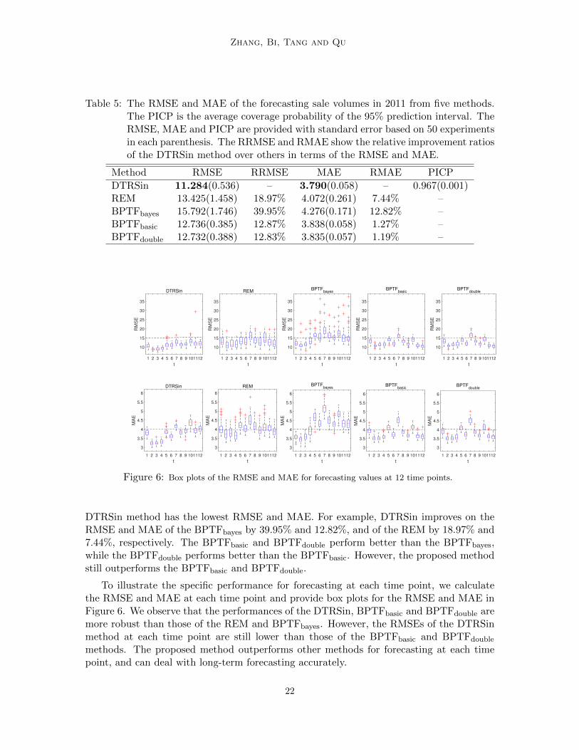
Figure 6: Box plots of the RMSE and MAE for forecasting values at 12 time points.
DTRSin method has the lowest RMSE and MAE. For example, DTRSin improves on theRMSE and MAE of the BPTFbayes by 39.95% and 12.82%, and of the REM by 18.97% and7.44%, respectively. The BPTFbasic and BPTFdouble perform better than the BPTFbayes,while the BPTFdouble performs better than the BPTFbasic. However, the proposed methodstill outperforms the BPTFbasic and BPTFdouble.
To illustrate the specific performance for forecasting at each time point, we calculatethe RMSE and MAE at each time point and provide box plots for the RMSE and MAE inFigure 6. We observe that the performances of the DTRSin, BPTFbasic and BPTFdouble aremore robust than those of the REM and BPTFbayes. However, the RMSEs of the DTRSinmethod at each time point are still lower than those of the BPTFbasic and BPTFdouble
methods. The proposed method outperforms other methods for forecasting at each timepoint, and can deal with long-term forecasting accurately.
22

Dynamic Tensor Recommender Systems
6.2 Last.fm Data
In this section, we analyze the Lastfm-1K dataset collected by Last.fm API (Celma, 2010)to evaluate the performance of the proposed method. The dataset is available at http:
//ocelma.net/MusicRecommendationDataset/lastfm-1K.html and has been widely usedin music recommendation experiments. The Lastfm data includes the listening history of992 users and songs played daily, recorded by quadruples with user, timestamp, artistand song information, where the users’ profiles contain gender, age, country and signup,and artists contain 107,528 artists with ID and 69,420 without ID. A detailed description ofthe Lastfm-1K dataset is available at http://ocelma.net/MusicRecommendationDataset/lastfm-1K.html.
We extract the user-artist-song playcount tensor-valued function with each monthlytime point based on the quadruples records. The goal of our study is to predict the futureplaycount of each song given each artist for each user. Through this prediction procedure,we are able to estimate future listening habit for each user, so that to recommend interestingsongs to each user. To evaluate the performance of the proposed method, we consider asub-dataset with 100 users randomly, where there are 7,490 artists, 32,287 songs and 53months from February of 2005 to June of 2009. We classify users, song, time stamp andartists into subgroups based on users’ gender, a song’s artist, month of the year, and whetherthe artist has ID, respectively. Although the observed records have been 356,786, thereare still a large number of user-artist-song-month combinations which are associated withunknown playcount. The data have a high missing rate and are highly sparse.
Similar to Section 6.1, we implement and report the performances of the proposedmethod and the competing methods. We randomly sample 80% of the data from Februaryof 2005 to May of 2008 (i.e., the first 40 months) as a training set and 20% of the datafrom June of 2008 to June of 2009 (i.e., the last 13 months) as the testing set. The randomsampling is replicated 50 times. Table 6 shows the forecasting results produced by eachmethod and the computational time.
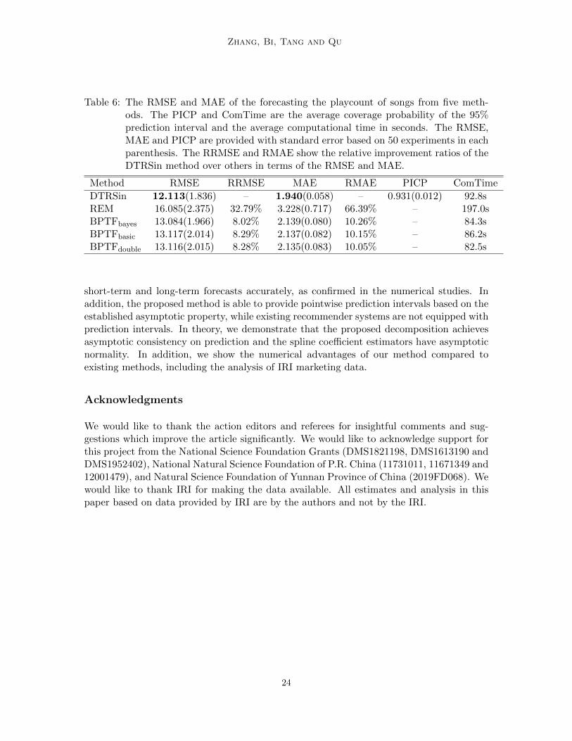
Table 6 indicates that the DTRSin method achieves coverage probabilities of the predic-tion interval close to 95%, which supports that the proposed method can obtain accurateprediction interval estimator, whereas the competing methods cannot provide such predic-tion interval. Table 6 also shows that the proposed method achieves the best performance.Specifically, the proposed method improves the compering methods by at least 8.02% withrespect to the RMSE, and by at least 10.05% with respect to the MAE, and still achievesthe smallest standard error with a reasonable computational time.
7. Discussion
In this article, we propose a new dynamic tensor recommender system which incorporatestime information through a tensor-valued function. A unique contribution of our methodis that it can estimate recommendation accurately given any time point in continuoustime intervals. Technically, the proposed method builds a time-value tensor decompositionmodel and borrows group information from existing time points of the same group for higherforecasting accuracy. Moreover, the proposed method utilizes the polynomial spline methodand the weighted least squared method to incorporate time-dependency and intra-clustercorrelation into the DRS. The spline extrapolation enables our method to achieve both
23
Zhang, Bi, Tang and Qu
Table 6: The RMSE and MAE of the forecasting the playcount of songs from five meth-ods. The PICP and ComTime are the average coverage probability of the 95%prediction interval and the average computational time in seconds. The RMSE,MAE and PICP are provided with standard error based on 50 experiments in eachparenthesis. The RRMSE and RMAE show the relative improvement ratios of theDTRSin method over others in terms of the RMSE and MAE.
Method RMSE RRMSE MAE RMAE PICP ComTime
DTRSin 12.113(1.836) – 1.940(0.058) – 0.931(0.012) 92.8sREM 16.085(2.375) 32.79% 3.228(0.717) 66.39% – 197.0sBPTFbayes 13.084(1.966) 8.02% 2.139(0.080) 10.26% – 84.3sBPTFbasic 13.117(2.014) 8.29% 2.137(0.082) 10.15% – 86.2sBPTFdouble 13.116(2.015) 8.28% 2.135(0.083) 10.05% – 82.5s
short-term and long-term forecasts accurately, as confirmed in the numerical studies. Inaddition, the proposed method is able to provide pointwise prediction intervals based on theestablished asymptotic property, while existing recommender systems are not equipped withprediction intervals. In theory, we demonstrate that the proposed decomposition achievesasymptotic consistency on prediction and the spline coefficient estimators have asymptoticnormality. In addition, we show the numerical advantages of our method compared toexisting methods, including the analysis of IRI marketing data.
Acknowledgments
We would like to thank the action editors and referees for insightful comments and sug-gestions which improve the article significantly. We would like to acknowledge support forthis project from the National Science Foundation Grants (DMS1821198, DMS1613190 andDMS1952402), National Natural Science Foundation of P.R. China (11731011, 11671349 and12001479), and Natural Science Foundation of Yunnan Province of China (2019FD068). Wewould like to thank IRI for making the data available. All estimates and analysis in thispaper based on data provided by IRI are by the authors and not by the IRI.
24
Dynamic Tensor Recommender Systems
Appendix A.
In this appendix we prove the theorems from Section 4.
Lemma 4 Predicted values given by (2) with fixed spline bases are invariant with respectto scaling and permutation indeterminacies.
Proof According to (2), the tensor function Y(t) is represented as:
Y(t) ≈r∑j=1
hj(t)p1·j p2
·j · · · pd·j + g(t)q1 q2 · · · qd.
Given fixed spline bases Bji(·)Mi=1, hj(t) is uniquely confirmed by coefficients αj forj = 1, . . . , r, and g(t) is similar. Thus, the determinacy of coefficients is equivalent tothe determinacy of functional factors, so we discuss the indeterminacy of functional fac-tors. Scaling indeterminacy refers to non-uniqueness with respect to a scale change ofpk·j and qk, and of each function hj(t) and g(t) for k = 1, . . . , d; j = 1, . . . , r. That is,
for πkl and δl, k = 1, . . . , d, l = 1, . . . , r + 1, we have pk·j = πkjpk·j , hj(t) = δjhj(t),
j = 1, . . . , r, qk = πkr+1qk, and g(t) = δr+1g(t) such that δl
∏dk=1 πkl = 1 for l =
1, . . . , r + 1. Thus, we know that∑r
j=1 hj(t)p1·j p2
·j · · · pd·j + g(t)q1 q2 · · · qd =∑rj=1 hj(t)p
1·j p2
·j · · · pd·j + g(t)q1 q2 · · · qd. Let h(t) = h1(t), h2(t), . . . , hr(t)>.Permutation indeterminacy refers to an arbitrary r × r permutation matrix Π such that∑r
j=1 hj(t)p1·j p2
·j · · · pd·j + g(t)q1 q2 · · · qd.= [[h(t); P1,P2, · · · ,Pd]] + g(t)q1 q2
· · · qd = [[Πh(t); P1Π,P2Π, · · · ,PdΠ]] + g(t)q1 q2 · · · qd. These imply the invarianceof equation (2) with respect to scaling and permutation indeterminacies. The proof of theLemma is completed.
Proof of Proposition 1.Based on the definition of Kruskal rank, the Kruskal rank of the (r + 1) × 1 matrix
(h1(t), h2(t), . . . , hr(t), g(t))> is one. Based on Theorem 3 in Sidiropoulos and Bro (2000),the sufficient condition of identifiability of (Pk,qk) up to permutation and scaling of columnsis∑d
k=1Kk + 1 ≥ 2(r + 1) + (d + 1) − 1, that is,∑d
k=1Kk ≥ 2r + d + 1. Under the
sufficient condition, if there exist two minimizers (P, q, α, β) and (P, q, α, β) of L(·|Y), then(P, q, α, β) and (P, q, α, β) are identical with the exception of scaling and permutation.By Lemma 4, the yi1i2···id ’s provided by (P, q, α, β) and (P, q, α, β) are identical. Thus,
L(P, q, α, β|Y) = L(P, q, α, β|Y) implies that∑dk=1(
∑rj=1 ‖pk·j‖22 + ‖qk‖22) +
∑rj=1 ‖αj‖2 +
∑md+1
e=1 ‖βe‖2
=∑d
k=1(∑r
j=1 ‖pk·j‖22 + ‖qk‖22) +∑r
j=1 ‖αj‖2 +∑md+1
e=1 ‖βe‖2.(12)
Suppose there exist some k1, k2 = 1, . . . , d, k1 6= k2, such that pk1·j = νjpk1·j , pk2·j = pk2·j /νj ,
qk1 = τ qk1 , qk2 = qk2/τ for positive constants τ, νj , j = 1, . . . , r. We have
r∑j=1
(‖pk1·j ‖22+‖pk2·j ‖
22)+‖qk1‖22+‖qk2‖22 =
r∑j=1
(ν2j ‖p
k1·j ‖
22+‖pk2·j ‖
22/ν
2j )+τ2‖qk1‖22+‖qk2‖22/τ2.
25

Zhang, Bi, Tang and Qu
Then (12) implies that τ = 1 and νj almost surely, j = 1, . . . , r. Similarly, suppose there
exist some k1 = 1, . . . , d, such that pk1·j = νjpk1·j , αj = αj/νj , qk1 = τ qk1 , βe = βe/τ for
positive constants τ, νj , j = 1, . . . , r; e = 1, . . . ,md+1. We have
∑rj=1(‖pk1·j ‖22 + ‖αj‖2) + ‖qk1‖22 +
∑md+1
e=1 ‖βe‖2
=∑r
j=1(ν2j ‖p
k1·j ‖22 + ‖αj‖2/ν2
j ) + τ2‖qk1‖22 +∑md+1
e=1 ‖βe‖2/τ2.
Then (12) implies that τ = 1 and νj almost surely, j = 1, . . . , r. Thus, (P, q, α, β) and
(P, q, α, β) are identical almost surely with the exception of permutation.
Proof of Theorem 2.
The estimator ui1···id is obtained by solving ∂(i1···id)L(U|Y) = 00, where ∂(i1···id) representsthe first derivatives with respect to the vector ui1···id . By Taylor expansion, we have
ui1···id − u0i1···id
= ∂2(i1···id)L(U|Y)|u∗i1···id
−1∂(i1···id)L(U|Y)|u0i1···id
= F>i1i2...idΣ−1i1i2...id
Fi1i2...id + λ∂2(i1···id)J(U)|u∗i1···id
−1
F>i1i2...idΣ−1i1i2...id
εi1i2...id − λ∂(i1···id)J(U)|u0i1···id
= I−11 I2
where u∗i1···id is between ui1···id and u0i1···id , and ∂2(i1···id) represents the second derivatives
with respect to the vector ui1···id . Since λ = op(1) and J(U) have bounded first and secondderivatives at true parameter U0, λ∂2
(i1···id)J(U)|u∗i1···id = op(1) and λ∂(i1···id)J(U)|u0i1···id=
op(1). Under conditions (C1), (C3) and (C4), we have
‖I1‖F = ‖F>i1i2...id(Σ−1i1i2...id
Σ0i1i2...id
)(Σ0i1i2...id
)−1Fi1i2...id + λ∂2(i1···id)J(U)|u∗i1···id‖F
≥ ‖c1σ−22 F>i1i2...idFi1i2...id + λ∂2
(i1···id)J(U)|u∗i1···id‖F≥ ‖c1σ
−22 mint∈Ti1...id
|Ti1...id | 1|Ti1...id
|∑
t∈Ti1...idf(t)f(t)>
+λ∂2(i1···id)J(U)|u∗i1···id‖F
& Tmin,
‖I2‖F ≤ ‖c2σ−21
∑t∈Ti1...id
f(t)εi1...idt − λ∂(i1···id)J(U)|u0i1···id‖F
≤ ‖Cc2σ−21 |Ti1...id | 1
|Ti1...id|∑
t∈Ti1...idεi1...idt − λ∂(i1···id)J(U)|u0i1···id
‖F
. |Ti1...id |1/2 . T1/2max,
where a . b and b & a mean a/b is bounded, Tmin = mint∈Ti1...id|Ti1...id | and Tmax =
maxt∈Ti1...id|Ti1...id |. Thus, under condition (C5), we have ‖ui1···id−u0i1···id‖2 . T
1/2max/Tmin
26

Dynamic Tensor Recommender Systems
. N τ/2−υ. Under condition (C1) and (C5), we have
1N
∑(i1,···,id)∈Ω ‖Fi1···id(ui1···id − u0i1···id)‖22
= 1N
∑(i1,···,id)∈Ω(ui1···id − u0i1···id)>
∑t∈Ti1...id
f(t)f(t)>(ui1···id − u0i1···id)
≤ C maxt∈Ti1...id|Ti1...id | 1
N
∑(i1,···,id)∈Ω(ui1···id − u0i1···id)>(ui1···id − u0i1···id)
. T 2max
NT 2min
. N−1+2(τ−υ).
The proof of Theorem 2 is completed.
We can currently use a convenient basis system in our technical arguments and theresults also hold true for other basis choices of the same function space. The B-spline andtruncated polynomial basis functions span the same set of spline functions (de Boor, 2001),thus we use B-splines as the convenient basis system in our proofs. The B-splines have thefollowing properties (de Boor, 2001): Bk(t) ≥ 0,
∑Mk=1Bk(t) = 1, t ∈ T, C1
M
∑Mk=1 φ
2kdt ≤∫
T(∑M
k=1 φkBk(t))2 ≤ C2
M
∑Mk=1 φ
2k, C1 and C2 are constant and φk ∈ R.
Lemma 5 Under Conditions (C1)-(C5), we have
1N
∑(i1,...,id)∈Ω(Wi1...id −Wi1...id)>Σ−1
i1...id(Wi1...id −Wi1...id) = Op(N
−1+2(τ−υ)),
1N
∑(i1,...,id)∈Ω(Wi1...id −Wi1...id)>Σ−1
i1...idWi1...id = Op(N
−1+3τ/2−υ),
1N
∑(i1,...,id)∈Ω(Wi1...id −Wi1...id)>Σ−1
i1...idεi1...id = Op(N
−1+τ−υ).
Proof By Theorem 2 and the non-negative bounded properties of the B-spline basis func-tions (de Boor, 2001), we have for j, l = 1, . . . , r; e, k = 1, . . . ,md+1,
1N
∑(i1,...,id)∈Ω(Xi1...idj −Xi1...idj)
>Σ−1i1...id
(Xi1...idl −Xi1...idl)
= 1N
∑(i1,...,id)∈Ω(ui1...idj − ui1...idj)(ui1...idl − ui1...idl)B>i1...idjΣ
−1i1...id
Bi1...idl
≤ c2σ−21 Tmax
1N
∑(i1,...,id)∈Ω(ui1...idj − ui1...idj)(ui1...idl − ui1...idl)
· 1|Ti1...id
|∑
t∈Ti1...idBj(t)
>Bl(t)
= Op(N−1+2(τ−υ)),
1N
∑(i1,...,id)∈Ω(Xi1...idj −Xi1...idj)
>Σ−1i1...id
(Zi1...ide − Zi1...ide)
≤ c2σ−21
1N
∑(i1,...,id)∈Ω(ui1...idj − ui1...idj)(ui1...id(r+1) − ui1...id(r+1))B
>i1...idj
Ai1...ide
= Op(N−1+2(τ−υ)),
and
1N
∑(i1,...,id)∈Ω(Zi1...idk − Zi1...idk)
>Σ−1i1...id
(Zi1...ide − Zi1...ide)
≤ c2σ−21
1N
∑(i1,...,id)∈Ω(ui1...id(r+1) − ui1...id(r+1))
2A>i1...idkAi1...ide = Op(N−1+2(τ−υ)).
27

Zhang, Bi, Tang and Qu
By definition, we have
1
N
∑(i1,...,id)∈Ω
(Wi1...id −Wi1...id)>Σ−1i1...id
(Wi1...id −Wi1...id) = Op(N−1+2(τ−υ)).
Under conditions (C3)-(C5), we have j, l = 1, . . . , r; e, k = 1, . . . ,md+1,
1N
∑(i1,...,id)∈Ω(Xi1...idj −Xi1...idj)
>Σ−1i1...id
Xi1...idl
≤ c2σ−21
1N
∑(i1,...,id)∈Ω(ui1...idj − ui1...idj)ui1...idlB>i1...idjBi1...idl
≤ c2σ−21 Tmax
1N
∑(i1,...,id)∈Ω(ui1...idj − ui1...idj)ui1...idl
1|Ti1...id
|∑
t∈Ti1...idBj(t)
>Bl(t)
= Op(N−1+3τ/2−υ),
1N
∑(i1,...,id)∈Ω(Xi1...idj −Xi1...idj)
>Σ−1i1...id
εi1...id
≤ c2σ−21
1N
∑(i1,...,id)∈Ω(ui1...idj − ui1...idj)B>i1...idjεi1...id
≤ CT1/2max
1N
∑(i1,...,id)∈Ω(ui1...idj − ui1...idj) 1
|Ti1...id|1/2∑
t∈Ti1...idεi1...idt
= Op(N−1+τ−υ),
1N
∑(i1,...,id)∈Ω(Xi1...idj −Xi1...idj)
>Σ−1i1...id
Zi1...ide = Op(N−1+3τ/2−υ),
1N
∑(i1,...,id)∈Ω(Zi1...ide − Zi1...ide)
>Σ−1i1...id
Xi1...idj = Op(N−1+3τ/2−υ),
1N
∑(i1,...,id)∈Ω(Zi1...ids − Zi1...ids)
>Σ−1i1...id
Zi1...ide = Op(N−1+3τ/2−υ),
1N
∑(i1,...,id)∈Ω(Zi1...ide − Zi1...ide)
>Σ−1i1...id
εi1...id = Op(N−1+τ−υ).
By definition, we can obtain
1
N
∑(i1,...,id)∈Ω
(Wi1...id −Wi1...id)>Σ−1i1...id
Wi1...id = Op(N−1+3τ/2−υ),
and1
N
∑(i1,...,id)∈Ω
(Wi1...id −Wi1...id)>Σ−1i1...id
εi1...id = Op(N−1+τ−υ).
Proof of Theorem 3Based on the criterion function (3), we can obtain the estimator of the coefficient as
follows:
γ = (∑
(i1,i2,...,id)∈Ω
W>i1i2...id
Σ−1i1i2...id
Wi1i2...id + λI)−1∑
(i1,i2,...,id)∈Ω
W>i1i2...id
Σ−1i1i2...id
yi1i2...id .
Thus, we have
γ − γ0 =(∑
(i1,...,id)∈Ω W>i1...id
Σ−1i1i2...id
Wi1...id/N + λI/N)−1∑
(i1,...,id)∈Ω W>i1...id
Σ−1i1i2...id
(yi1...id − Wi1...idγ0)/N − λγ0/N.
28

Dynamic Tensor Recommender Systems
By Lemma 5, we have
1N
∑(i1,...,id)∈Ω W>
i1...idΣ−1i1i2...id
Wi1...id
= 1N
∑(i1,...,id)∈Ω W>
i1...idΣ−1i1i2...id
Wi1...id
+ 1N
∑(i1,...,id)∈Ω(Wi1...id −Wi1...id)>Σ−1
i1i2...id(Wi1...id −Wi1...id)
+ 1N
∑(i1,...,id)∈Ω(Wi1...id −Wi1...id)>Σ−1
i1i2...idWi1...id
+ 1N
∑(i1,...,id)∈Ω W>
i1...idΣ−1i1i2...id
(Wi1...id −Wi1...id)
= 1N
∑(i1,...,id)∈Ω W>
i1...idΣ−1i1i2...id
Wi1...id +Op(N−1+3τ/2−υ)
and
1N
∑(i1,...,id)∈Ω W>
i1...idΣ−1i1i2...id
(yi1...id − Wi1...idγ0)
= 1N
∑(i1,...,id)∈Ω W>
i1...idΣ−1i1i2...id
(yi1...id −Wi1...idγ0)
− 1N
∑(i1,...,id)∈Ω(Wi1...id −Wi1...id)>Σ−1
i1i2...id(Wi1...id −Wi1...id)γ0
+ 1N
∑(i1,...,id)∈Ω(Wi1...id −Wi1...id)>Σ−1
i1i2...id(yi1...id −Wi1...idγ0)
− 1N
∑(i1,...,id)∈Ω W>
i1...idΣ−1i1i2...id
(Wi1...id −Wi1...id)γ0
= 1N
∑(i1,...,id)∈Ω W>
i1...idΣ−1i1i2...id
(yi1...id −Wi1...idγ0)
+ 1N
∑(i1,...,id)∈Ω(Wi1...id −Wi1...id)>Σ−1
i1i2...id(yi1...id −Wi1...idγ0) +Op(N
−1+3τ/2−υ).
According to de Boor (2001), supt∈T |hj(t)− hj(t)| ≤ Ca−ξN and supt∈T |ge(t)− ge(t)| ≤
Ca−ξN for each j = 1, . . . , r and each e = 1, . . . ,md+1, where hj(t) = α>0jBj(t) and
ge(t) = β>0eAe(t). Let yi1...id = Wi1...idγ0 =∑r
j=1 ui1...idjhi1...idj + ui1...id(r+1)gi1...id ,
yi1...id =∑r
j=1 ui1...idjhi1...idj + ui1...id(r+1)gi1...id , where hi1...idj = Bi1i2...idjα0j , gi1...id =∑md+1
e=1 Ai1i2...ideβ0e, and hi1...idj and gi1...id consist of hj(t) and g(t) for all t ∈ Ti1...id , re-spectively. That is, yi1...id = yi1...id +εi1...id . Similar to the proof of lemma 5, we can obtainthat
1
N
∑(i1,...,id)∈Ω
W>i1...id
Σ−1i1i2...id
r∑j=1
ui1...idj(hi1...idj − hi1...idj) = Op(a−ξN N τ−1),
and
1
N
∑(i1,...,id)∈Ω
W>i1...id
Σ−1i1i2...id
(gi1...id − gi1...id)ui1...id(r+1) = Op(a−ξN N τ−1).
29

Zhang, Bi, Tang and Qu
Therefore, we have
1N
∑(i1,...,id)∈Ω W>
i1...idΣ−1i1i2...id
(yi1...id −Wi1...idγ0)
= 1N
∑(i1,...,id)∈Ω W>
i1...idΣ−1i1i2...id
(yi1...id − yi1...id)
+ 1N
∑(i1,...,id)∈Ω W>
i1...idΣ−1i1i2...id
(yi1...id − yi1...id)
= 1N
∑(i1,...,id)∈Ω W>
i1...idΣ−1i1i2...id
εi1...id
+ 1N
∑(i1,...,id)∈Ω W>
i1...idΣ−1i1i2...id
∑r
j=1 ui1...idj(hi1...idj − hi1...idj)
+ 1N
∑(i1,...,id)∈Ω W>
i1...idΣ−1i1i2...id
(gi1...id − gi1...id)ui1...id(r+1)
= 1N
∑(i1,...,id)∈Ω W>
i1...idΣ−1i1i2...id
εi1...id + op(a−ξN N τ−1).
Similarly, we can obtain
1N
∑(i1,...,id)∈Ω(Wi1...id −Wi1...id)>Σ−1
i1i2...id(yi1...id −Wi1...idγ0)
= 1N
∑(i1,...,id)∈Ω(Wi1...id −Wi1...id)>Σ−1
i1i2...idεi1...id
+ 1N
∑(i1,...,id)∈Ω(Wi1...id −Wi1...id)>Σ−1
i1i2...id∑r
j=1 ui1...idj(hi1...idj − hi1...idj)
+ 1N
∑(i1,...,id)∈Ω(Wi1...id −Wi1...id)>Σ−1
i1i2...id(gi1...id − gi1...id)ui1...id(r+1)
= Op(N−1+τ−υ) +Op(a
−ξN N−1+3τ/2−υ).
Thus, we have
1N
∑(i1,...,id)∈Ω W>
i1...idΣ−1i1i2...id
(yi1...id − Wi1...idγ0)
= 1N
∑(i1,...,id)∈Ω W>
i1...idΣ−1i1i2...id
εi1...id + op(N−1+τ−υ) + op(a
−ξN N τ−1).
Since λ = op(1), we have N−1λI = op(N−1) and N−1λγ0 = op(N
−1). Then, we have
1N
∑(i1,...,id)∈Ω W>
i1...idΣ−1i1i2...id
Wi1...id + 1N λI
= 1N
∑(i1,...,id)∈Ω W>
i1...idΣ−1i1i2...id
Wi1...id + op(N−1+3τ/2−υ),
and
1N
∑(i1,...,id)∈Ω W>
i1...idΣ−1i1i2...id
(yi1...id − Wi1...idγ0)− 1N λγ0
= 1N
∑(i1,...,id)∈Ω W>
i1...idΣ−1i1i2...id
εi1...id + op(N−1+τ−υ) + op(a
−ξN N τ−1).
For any vector c whose components are not all zero, we have
c>(γ − γ0)
=∑
(i1,...,id)∈Ω c>(∑
(i1,...,id)∈Ω W>i1...id
Σ−1i1i2...id
Wi1...id)−1W>i1...id
Σ−1i1i2...id
εi1...id + op(1)
=∑
(i1,...,id)∈Ω ai1...idζi1...id + op(1),
where ζi1...id are independent with mean zero and variance one given Wi1...id , (i1, . . . , id) ∈Ω, and
a2i1...id
= c>(∑
(i1,...,id)∈Ω W>i1...id
Σ−1i1i2...id
Wi1...id)−1W>i1...id
Σ−1i1i2...id
Σ0i1...id
Σ−1i1i2...id
Wi1...id
(∑
(i1,...,id)∈Ω W>i1...id
Σ−1i1i2...id
Wi1...id)−1c.
30

Dynamic Tensor Recommender Systems
It follows easily by checking the Lindeberg condition that if
max(i1,...,id)∈Ω a2i1...id∑
(i1,...,id)∈Ω a2i1...id
→p 0, (13)
then∑
(i1,...,id)∈Ω ai1...idζi1...id/√∑
(i1,...,id)∈Ω a2i1...id
is asymptotically N(0, 1). We only need
to show that (13) holds.
Based on the properties of the B-splines and conditions (C3)-(C4), we have, for anyφ = (φ>1, . . . ,φ
>r+md+1
)> with φj ∈ RM ,
φ>W>i1...id
Σ−1i1i2...id
Σ0i1...id
Σ−1i1i2...id
Wi1...idφ
≤ c22σ−21
∑t∈Ti1...id
(φ>wi1...idt)2
= c22σ−21
∑t∈Ti1...id
∑r
j=1 ui1i2...idjφ>jBj(t) + ui1i2...id(r+1)
∑md+1
e=1 φ>r+eAe(t)I(t ∈ se)2
≤ cc22σ−21
∑t∈Ti1...id
[(∑r
j=1 u2i1i2...idj
)∑r
j=1φ>jBj(t)2 + u2
i1i2...id(r+1)
∑md+1
e=1 φ>r+eAe(t)2]
. (∑r
j=1 u2i1i2...idj
)∑r
j=1
∑t∈Ti1...id
φ>jBj(t)2 + u2i1i2...id(r+1)
∑md+1
e=1
∑t∈Ti1...id
φ>r+eAe(t)2
. (∑r
j=1 u2i1i2...idj
)∑r
j=1C2M |φj |
2 + u2i1i2...id(r+1)
∑md+1
e=1C2M |φr+e|
2
. (∑r+1
j=1 u2i1i2...idj
)C2M |φ|
2
. 1M |φ|
2.
By Lemmas A.1 and A.2 in Huang et al. (2004), we have
φ>(∑
(i1,...,id)∈Ω W>i1...id
Σ−1i1i2...id
Σ0i1...id
Σ−1i1i2...id
Wi1...id)φ
≥ c21σ−22
∑(i1,...,id)∈Ωφ
>W>i1...id
Wi1...idφ
≥ c21σ−22 NTmin[ 1
N
∑(i1,...,id)∈Ω
1|Ti1...id
|∑
t∈Ti1...id∑r
j=1 ui1i2...idjφ>jBj(t)
+ui1i2...id(r+1)
∑md+1
e=1 φ>r+eAe(t)I(t ∈ se)2]
≥ c21σ−22 NTmin[ 1
N
∑(i1,...,id)∈Ω
1|Ti1...id
|∑
t∈Ti1...id∑r
j=1 ui1i2...idjφ>jBj(t)
+ mineui1i2...id(r+1)φ>r+eAe(t)2]
& NTmin1M |φ|
2.
Thus, we obtain that
max(i1,...,id)∈Ωφ>W>
i1...idΣ−1i1i2...id
Σ0i1...id
Σ−1i1i2...id
Wi1...idφ
φ>(∑
(i1,...,id)∈Ω W>i1...id
Σ−1i1i2...id
Σ0i1...id
Σ−1i1i2...id
Wi1...id)φ.
1
NTmin.
Hence, (13) holds. Then we have c>(γ−γ0)varc>(γ−γ0)−1/2 L→ N(0, 1), where varc>(γ−γ0) = c>Ψ−1ΦΨ−1c, in which Φ =
∑(i1,...,id)∈Ω W>
i1...idΣ−1i1i2...id
Σ0i1...id
Σ−1i1i2...id
Wi1...id , and
Ψ =∑
(i1,...,id)∈Ω W>i1...id
Σ−1i1i2...id
Wi1...id .
31
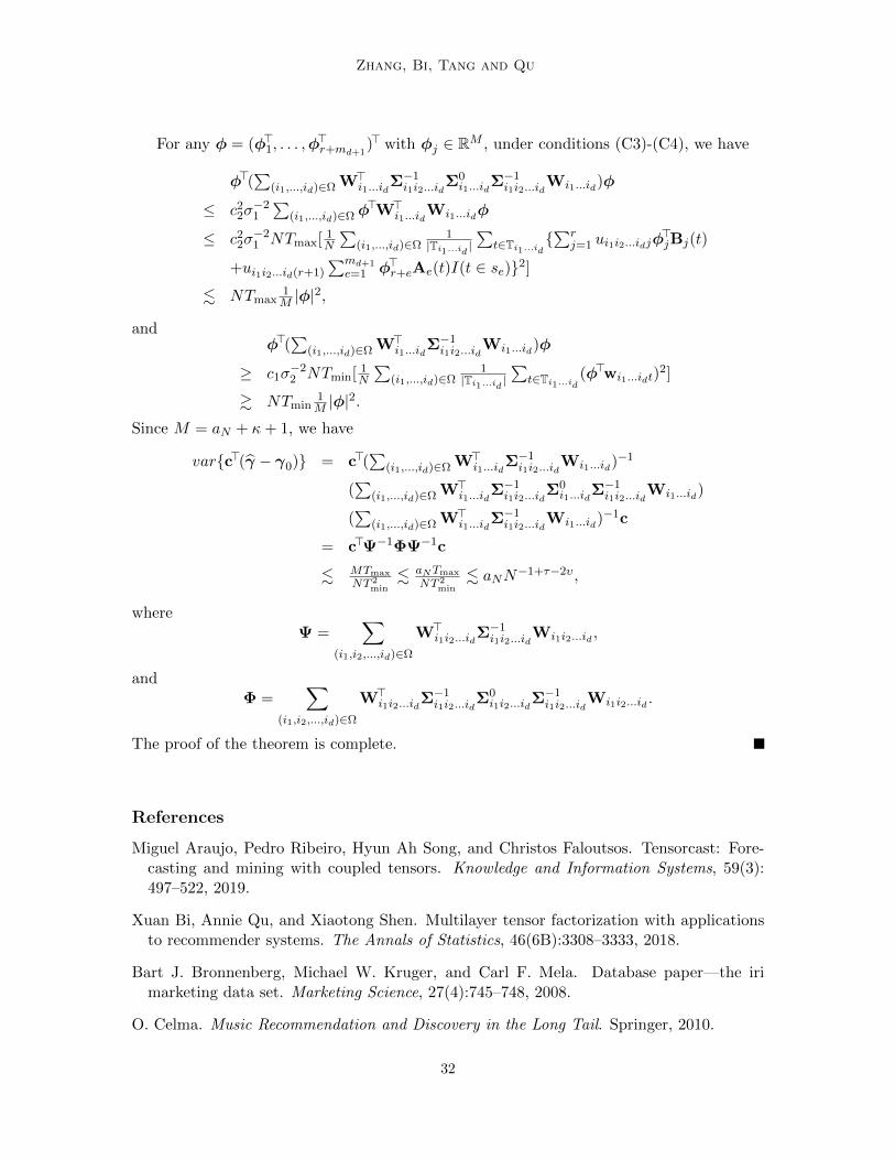
Zhang, Bi, Tang and Qu
For any φ = (φ>1, . . . ,φ>r+md+1
)> with φj ∈ RM , under conditions (C3)-(C4), we have
φ>(∑
(i1,...,id)∈Ω W>i1...id
Σ−1i1i2...id
Σ0i1...id
Σ−1i1i2...id
Wi1...id)φ
≤ c22σ−21
∑(i1,...,id)∈Ωφ
>W>i1...id
Wi1...idφ
≤ c22σ−21 NTmax[ 1
N
∑(i1,...,id)∈Ω
1|Ti1...id
|∑
t∈Ti1...id∑r
j=1 ui1i2...idjφ>jBj(t)
+ui1i2...id(r+1)
∑md+1
e=1 φ>r+eAe(t)I(t ∈ se)2]
. NTmax1M |φ|
2,
andφ>(∑
(i1,...,id)∈Ω W>i1...id
Σ−1i1i2...id
Wi1...id)φ
≥ c1σ−22 NTmin[ 1
N
∑(i1,...,id)∈Ω
1|Ti1...id
|∑
t∈Ti1...id(φ>wi1...idt)
2]
& NTmin1M |φ|
2.
Since M = aN + κ+ 1, we have
varc>(γ − γ0) = c>(∑
(i1,...,id)∈Ω W>i1...id
Σ−1i1i2...id
Wi1...id)−1
(∑
(i1,...,id)∈Ω W>i1...id
Σ−1i1i2...id
Σ0i1...id
Σ−1i1i2...id
Wi1...id)
(∑
(i1,...,id)∈Ω W>i1...id
Σ−1i1i2...id
Wi1...id)−1c
= c>Ψ−1ΦΨ−1c
. MTmax
NT 2min
. aNTmax
NT 2min
. aNN−1+τ−2υ,
whereΨ =
∑(i1,i2,...,id)∈Ω
W>i1i2...id
Σ−1i1i2...id
Wi1i2...id ,
andΦ =
∑(i1,i2,...,id)∈Ω
W>i1i2...id
Σ−1i1i2...id
Σ0i1i2...id
Σ−1i1i2...id
Wi1i2...id .
The proof of the theorem is complete.
References
Miguel Araujo, Pedro Ribeiro, Hyun Ah Song, and Christos Faloutsos. Tensorcast: Fore-casting and mining with coupled tensors. Knowledge and Information Systems, 59(3):497–522, 2019.
Xuan Bi, Annie Qu, and Xiaotong Shen. Multilayer tensor factorization with applicationsto recommender systems. The Annals of Statistics, 46(6B):3308–3333, 2018.
Bart J. Bronnenberg, Michael W. Kruger, and Carl F. Mela. Database paper—the irimarketing data set. Marketing Science, 27(4):745–748, 2008.
O. Celma. Music Recommendation and Discovery in the Long Tail. Springer, 2010.
32
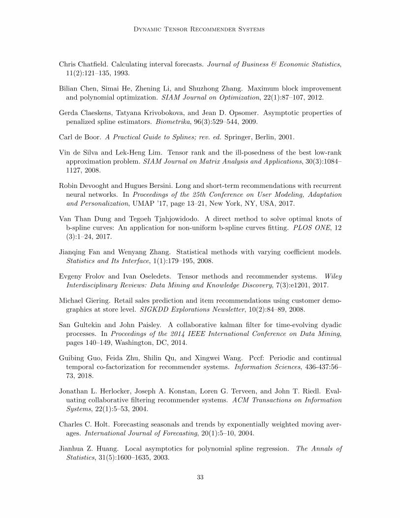
Dynamic Tensor Recommender Systems
Chris Chatfield. Calculating interval forecasts. Journal of Business & Economic Statistics,11(2):121–135, 1993.
Bilian Chen, Simai He, Zhening Li, and Shuzhong Zhang. Maximum block improvementand polynomial optimization. SIAM Journal on Optimization, 22(1):87–107, 2012.
Gerda Claeskens, Tatyana Krivobokova, and Jean D. Opsomer. Asymptotic properties ofpenalized spline estimators. Biometrika, 96(3):529–544, 2009.
Carl de Boor. A Practical Guide to Splines; rev. ed. Springer, Berlin, 2001.
Vin de Silva and Lek-Heng Lim. Tensor rank and the ill-posedness of the best low-rankapproximation problem. SIAM Journal on Matrix Analysis and Applications, 30(3):1084–1127, 2008.
Robin Devooght and Hugues Bersini. Long and short-term recommendations with recurrentneural networks. In Proceedings of the 25th Conference on User Modeling, Adaptationand Personalization, UMAP ’17, page 13–21, New York, NY, USA, 2017.
Van Than Dung and Tegoeh Tjahjowidodo. A direct method to solve optimal knots ofb-spline curves: An application for non-uniform b-spline curves fitting. PLOS ONE, 12(3):1–24, 2017.
Jianqing Fan and Wenyang Zhang. Statistical methods with varying coefficient models.Statistics and Its Interface, 1(1):179–195, 2008.
Evgeny Frolov and Ivan Oseledets. Tensor methods and recommender systems. WileyInterdisciplinary Reviews: Data Mining and Knowledge Discovery, 7(3):e1201, 2017.
Michael Giering. Retail sales prediction and item recommendations using customer demo-graphics at store level. SIGKDD Explorations Newsletter, 10(2):84–89, 2008.
San Gultekin and John Paisley. A collaborative kalman filter for time-evolving dyadicprocesses. In Proceedings of the 2014 IEEE International Conference on Data Mining,pages 140–149, Washington, DC, 2014.
Guibing Guo, Feida Zhu, Shilin Qu, and Xingwei Wang. Pccf: Periodic and continualtemporal co-factorization for recommender systems. Information Sciences, 436-437:56–73, 2018.
Jonathan L. Herlocker, Joseph A. Konstan, Loren G. Terveen, and John T. Riedl. Eval-uating collaborative filtering recommender systems. ACM Transactions on InformationSystems, 22(1):5–53, 2004.
Charles C. Holt. Forecasting seasonals and trends by exponentially weighted moving aver-ages. International Journal of Forecasting, 20(1):5–10, 2004.
Jianhua Z. Huang. Local asymptotics for polynomial spline regression. The Annals ofStatistics, 31(5):1600–1635, 2003.
33
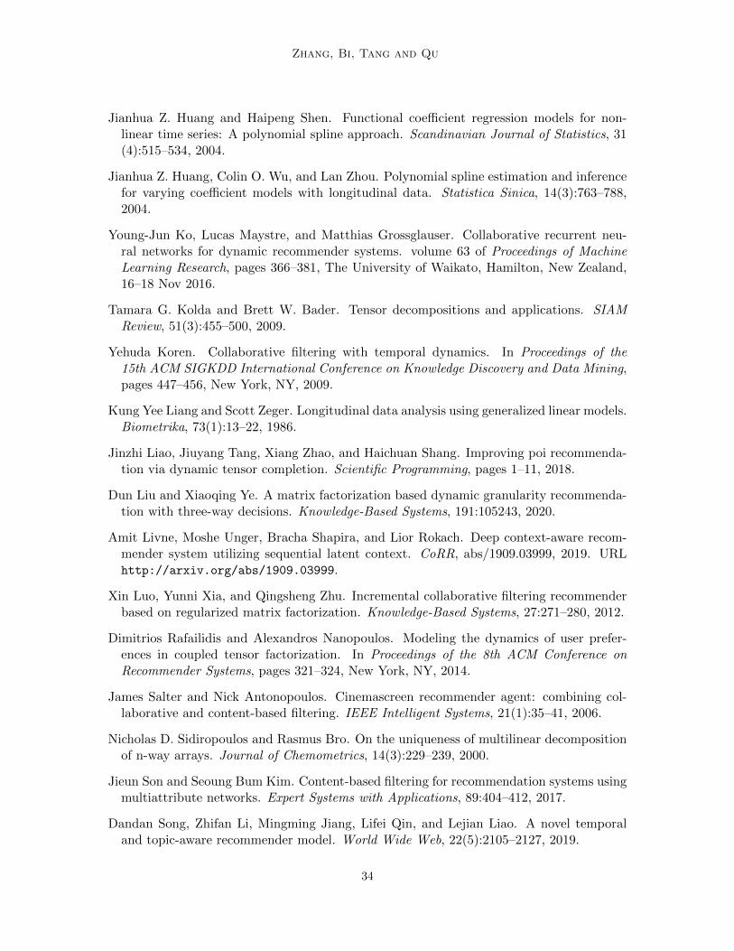
Zhang, Bi, Tang and Qu
Jianhua Z. Huang and Haipeng Shen. Functional coefficient regression models for non-linear time series: A polynomial spline approach. Scandinavian Journal of Statistics, 31(4):515–534, 2004.
Jianhua Z. Huang, Colin O. Wu, and Lan Zhou. Polynomial spline estimation and inferencefor varying coefficient models with longitudinal data. Statistica Sinica, 14(3):763–788,2004.
Young-Jun Ko, Lucas Maystre, and Matthias Grossglauser. Collaborative recurrent neu-ral networks for dynamic recommender systems. volume 63 of Proceedings of MachineLearning Research, pages 366–381, The University of Waikato, Hamilton, New Zealand,16–18 Nov 2016.
Tamara G. Kolda and Brett W. Bader. Tensor decompositions and applications. SIAMReview, 51(3):455–500, 2009.
Yehuda Koren. Collaborative filtering with temporal dynamics. In Proceedings of the15th ACM SIGKDD International Conference on Knowledge Discovery and Data Mining,pages 447–456, New York, NY, 2009.
Kung Yee Liang and Scott Zeger. Longitudinal data analysis using generalized linear models.Biometrika, 73(1):13–22, 1986.
Jinzhi Liao, Jiuyang Tang, Xiang Zhao, and Haichuan Shang. Improving poi recommenda-tion via dynamic tensor completion. Scientific Programming, pages 1–11, 2018.
Dun Liu and Xiaoqing Ye. A matrix factorization based dynamic granularity recommenda-tion with three-way decisions. Knowledge-Based Systems, 191:105243, 2020.
Amit Livne, Moshe Unger, Bracha Shapira, and Lior Rokach. Deep context-aware recom-mender system utilizing sequential latent context. CoRR, abs/1909.03999, 2019. URLhttp://arxiv.org/abs/1909.03999.
Xin Luo, Yunni Xia, and Qingsheng Zhu. Incremental collaborative filtering recommenderbased on regularized matrix factorization. Knowledge-Based Systems, 27:271–280, 2012.
Dimitrios Rafailidis and Alexandros Nanopoulos. Modeling the dynamics of user prefer-ences in coupled tensor factorization. In Proceedings of the 8th ACM Conference onRecommender Systems, pages 321–324, New York, NY, 2014.
James Salter and Nick Antonopoulos. Cinemascreen recommender agent: combining col-laborative and content-based filtering. IEEE Intelligent Systems, 21(1):35–41, 2006.
Nicholas D. Sidiropoulos and Rasmus Bro. On the uniqueness of multilinear decompositionof n-way arrays. Journal of Chemometrics, 14(3):229–239, 2000.
Jieun Son and Seoung Bum Kim. Content-based filtering for recommendation systems usingmultiattribute networks. Expert Systems with Applications, 89:404–412, 2017.
Dandan Song, Zhifan Li, Mingming Jiang, Lifei Qin, and Lejian Liao. A novel temporaland topic-aware recommender model. World Wide Web, 22(5):2105–2127, 2019.
34

Dynamic Tensor Recommender Systems
W. Van Loock, G. Pipeleers, J. De Schutter, and J. Swevers. A convex optimization ap-proach to curve fitting with b-splines. IFAC Proceedings Volumes, 44(1):2290–2295, 2011.
Jian Wei, Jianhua He, Kai Chen, Yi Zhou, and Zuoyin Tang. Collaborative filtering anddeep learning based recommendation system for cold start items. Expert Systems withApplications, 69:29–39, 2017.
Peter R. Winters. Forecasting sales by exponentially weighted moving averages. Manage-ment Science, 6(3):324–342, 1960.
Chao-Yuan Wu, Amr Ahmed, Alex Beutel, Alexander J. Smola, and How Jing. Recurrentrecommender networks. In Proceedings of the Tenth ACM International Conference onWeb Search and Data Mining, pages 495–503, New York, NY, 2017.
Xian Wu, Baoxu Shi, Yuxiao Dong, Chao Huang, and Nitesh V. Chawla. Neural tensorfactorization for temporal interaction learning. In Proceedings of the Twelfth ACM In-ternational Conference on Web Search and Data Mining, pages 537–545, New York, NY,2019.
Liang Xiong, Xi Chen, Tzu-Kuo Huang, Jeff Schneider, and Jaime G Carbonell. Temporalcollaborative filtering with bayesian probabilistic tensor factorization. In Proceedings ofthe 2010 SIAM International Conference on Data Mining, pages 211–222, 2010.
Lan Xue and Lijian Yang. Additive coefficient modeling via polynomial spline. StatisticaSinica, 16(4):1423–1446, 2006.
Hsiang-Fu Yu, Nikhil Rao, and Inderjit S Dhillon. Temporal regularized matrix factoriza-tion for high-dimensional time series prediction. In D. Lee, M. Sugiyama, U. Luxburg,I. Guyon, and R. Garnett, editors, Advances in Neural Information Processing Systems,volume 29, pages 847–855. Curran Associates, Inc., 2016.
Yuan Yuan, Nan Chen, and Shiyu Zhou. Adaptive b-spline knot selection using multi-resolution basis set. IIE Transactions, 45(12):1263–1277, 2013.
Chenyi Zhang, Ke Wang, Hongkun Yu, Jianling Sun, and Ee-Peng Lim. Latent factor tran-sition for dynamic collaborative filtering. In Proceedings of the 2014 SIAM InternationalConference on Data Mining, pages 452–460, 2014.
35


![A Fuzzy Recommender System for eElections - unifr.ch Fuzzy Recommender System for eElections 63 2 Recommender Systems for eCommerce According to Yager [4], recommender systems used](https://img.dokumen.tips/doc/110x75/5b08be647f8b9a93738cdc60/a-fuzzy-recommender-system-for-eelections-unifrch-fuzzy-recommender-system-for.jpg)