Embed Size (px)
Citation preview
DYNAMIC STABILITY OF PLATES BY
FINITE ELEMENTS
By
JOHNNY MACK BUTT {/
Bacheler of Science University of Alabama University, Alabama
1963
Maeter of Science University of Alabama University, Alabama
1965
Submitted te the faculty of the Graduate College @f the Oklahoma State University
in partial fulfillment of the requirements fer the degree of
DOCTOR OF PHILOSOPHY May, 1968

DYNAMIC STABILITY OF PLATES BY
FINITE ELEMENTS
Thesis Approved:
Dean of the Graduate College
ii
OKLAHOMA STATE UNJVERSIJY LIBRARY
OCT 25 1968

ACKNOWLEDGMENTS
The author wishes te express his gratitude and sincere apprecia-
tion to the following individuals and organizations:
To Professor Ahmed E. Salama for his advice and friendship in the
preparation of this thesis;
To Professor Jan J. Tuma for serving as chairman of the advisory
committee and for his inspirational teaching and guidance;
To the members of the advisory committee, Professors Ahmed E.
Salama, Donald E. Boyd, Anthony F. Gaudy, and Thomas s. Dean
for their guidance and encouragement;
To the Civil Engineering Department at Oklahoma State University
and the Natienal Science Foundation for providing the oppor-
tunity for financial assistance;
To the staffs of the University Computer Center and the University
Library for their invaluable assistance;
To Mr. Eldon Hardy for preparing the final sketches;
To his wife, Mary Elaine, and daughter, Lisa, fer their patient
understanding, encouragement, and assistance;
To Mrs. Donna DeFrain, who typed the manuscript.
May, 1968 Stillwater, Oklahema
iii
Johnny Mack Hutt

Chapter
I.
u.
III.
TABLE OF CONTENTS
INTRODUCTION • • • "' . . . . . . . • • • • • • • • • •
1.1 Statement of the Problem ••••••••••• 1,2 Review of Previous Work ••••••••••• 1.3 Scope ••.••••••••••••••••••
• •
• • • • • •
GOVERNING FINITE El.EMENT EQUATIONS. • • • • • • • I I I I
Page
1
1 2 3
6
2.1 Ki~etic Energy. • • • • • • • • • • • • • • • • • 8 2.2 Strain Energy. • • • • • • • • • • • • • • • • • 10 2.3 Work Done by In-Plane Loads. • • • • • • • • • • 11 2.4 Damping and Elastic Foundation. • • • • • • • • • 13 2.5 Governing Equations • • • • • • • • • • • • • • • 14 2. 6 Development of Elemental Matrices • • • • • • • • 16
BOUNDARIES OF STABILITY FOR LINEAR EQUATIONS WITH PERIODIC COEFFICIENTS •••••••••••••• • • . . .
3.1 3.2 3.3 3.4 3.5 3.6
Behavior of Solutions •• • • • • • • • • • • • • Roots of Ch~racteristic Equation ••••••••• Regions of Stability and Instability ••••••• Boundary Frequencies for Instability ••••••• Equations With Damping Terms ••••••••••• Physical Considerations •••••••••••••
26
26 31 32 34 37 38
IV., SOLUTION FOR 'I'HE REGIONS OF DYNAMIC INSTABILITY. • • • o e 40
v.
4.1 Formulation of the Structural Matrices. • • • • • 42 l~. 2 Boundary Conditions • , • • , • • • • • • • • • • 43 4 • 3 . So 1 u ti on. ti • • • • • , • • • • • o • • • • • • • 4 5
DISCUSSION OF RESULTS. • • . . . . . . I • 0 . . . • • • •
5.1 Interpretation of Results •••••••••••• 5.2 Plates Without Damping •••••••••••••• 5.3 Plates on Elastic Foundations ••••••••• , 5.4 Plates With Viscous Damping ••••••• 5.5 Plate on Elastic Foundation With Viscous
Damping ••••••••• • • • • • • 41
iv
• • • •
. . . .
48
48 49 68 79
79

TABLE OF' CONTJ~NTS (Continued)
Chapter Page
VI. SUMMARY AND CONCLUSIONS. G • • • • • • • • 0 • • • • • • • 83
6 .1 Summary and Conclusions • • • • • • • • • • • • • 83 6.2 Suggestion for Further Research. • • • • • • • • 84
BIBLIOGRAPHY. • • • o • o ~ • o a o • • o • • • o • • • • • • • • 86
v

LIST OF TABLES
Table Page
l, Mode Shapes, Natural Frequencies, and Buckling Loads for
Il.
Several Plates. • • • • • • • • • • • • • • • • • • • • 54
Information for Obtaining the Fundamental Region of Instability for Several Plates • • • • • • • • • •
vi
• • • 55

LIST OF FIGURES
Figure Page
1. Finite Element With Generalized Coordinates •• • • • • • • • 16
2. Generalized Coordinates, Function of Constants. • • • • • • 18
3. [EJ and [G] Matrices •• • • • • • • • • • • • • . . . • • • 19
4. Elemental Mass Matrix. • • • • • • • • • • • • • • • • • • • 21
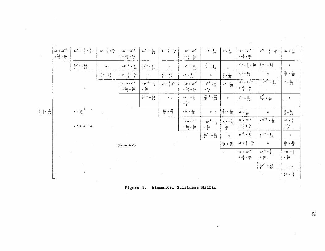
s. Elemental Stiffness Matrix •• • • • • • • • • • • • • • • • 22
6. Elemental Stability Matrix for Nx• ••••••• ·.• • • • • • 23
Elemental Stability Matrix for N •• y 7. • • • 24 • • • • • • • • •
8. Elemental Stability Matrix for Nxy. • • • • • • • • • • 25
9. Nature of Vibrations. • • • • • • • • • • • • • • • • • • • 39
10. General Problem ••• • • • • • • • • • • • • • • • • • • • • 41
11. Regions of Dynamic Instability. • • . . • • • • • • • • • • 51
12. Instability Regions for Mathieu Equation. • • . . . . . . . 52
13. Regions of Dynamic Instability for a Simply Supported Plate (N = N, Nx = O, N = O) ••••••••• , • • • • • • • 59 xy y
14. Mode Shapes for a Simply Supported Plate (Nxy = N) • • • • • 60
15. Regions of Dynamic Instability for a Simply Supported Plate (Nx = .lN, Ny= ,lN, ~y = N) •• , •••••••• , •• , 61
16, Mode Shapes for a Simply Supported Plate (Nx = .lN, Ny= • lN, Nxy = N). • • • • • • • • • • • • • • • • • • • • • • 62
17. Regions of Dynamic Instability for a Cantilevered Pl~te {Ny= N) •••••••••• • • • • , • , • • • • • • • • 64
18. Mode Shapes for a Cantilevered Plate (Ny= N) ••••• , • • 65
19. Regions of Dynamic Instability for a Fixed Ended Plate (Ny = N) • • • • • • • • • • • • • , • • , , • • • • • • • 66
vii

Figure
20.
21.
22.
23.
24.
25.
26.
';.7.
28.
29.
30.
• • • Mode Shapes for a Fixed Ended Plate (Ny= N) •••••
Regions of Dynamic Instability for a Simply Supported Plate on an Elastic Foundation (8 = .0002, a= O) •• • • •
Regions of Dynamic Instability for a Simply Supported Plate on an Elastic Foundation(~= .0002, a= 0.6), • • •
Mede Shapes for a Sim.ply Supported Plate on an Elastic Foundation(~= .0002, N = N = N) •••••••••
x y • • •
Regions of Dynamic Instability for a Simply Supported Plate on an Elastic Foundation(~= .0006, a= O) •• • • •
Regions of Dynamic Instability for a Simply Supported Plate on an Elastic Foundation(~= ,0006, a= 0,6). • • •
Mode Shapes for a Simply Supported Plate on an ~lastic Foundation(~= .0006, Nx =Ny= N) ••••••••• • • •
Regions of Dynamic Instability for a Clamped Plate on an Elastic.Foundation(~= ,0002) ••• , , , •• , •••
Mode Shapes for a Cl.amped Plate on an Elastic Foundation (~ = .0002~ Nx =Ny= N) •• , ••• , • , ••••••
Regions of Dynamic Instability for a Clamped Plate on an Elastic Foundation(~= .0006) • • • • • • • ••
Mode Shapes for a Clamped Plate on an Elastic Foundation (S = • 0006. Nlr = N = N) • • • • • • • • • • • • • , •
--- y
• •
• •
• •
• •
31. Regions of Dynamic Instability for a Simply Supported Plate
Page
67
69
70
71
72
73
74
75
76
77
78
With Viscous Damping • • • • • • • • • • • • • • • • • • • 80
32. Regions of Dynmn:i.c Instability for a Clamped Plate With Viscous Damping. • • • • • • • • • • • • • • • • • 81
33. Region of Dynamic Instability for a Simply Supported Plate on an Elastic Foundation With Viscous Damping. • • • • • • 82
viii

NOMENCLATURE
a ••••••••••• plate dimension in the x-direction, also a constant
A1 , aij' a •••••• constants
{.A}, [A], {ak1 • • • • constant matrices
b. 0 0 • 0 • • . . . . • • 0 • • •
I O . . . . . . . . . • • • • • • •
[BJ. • 0 • • • • . . .
plate dimension in they-direction, also a constant
constants
constant vector
constant matrix which relates {A} to the node di.splacements
periodic matrilc
c ••••••••••• damping ~oefficient
Co • • • • o o o • • • constant
le}. ......... matrix of second partial derivatives of w
C~j ••••••••• nodal carry-over stiffness matrix
d. • • • • • • • • • •
D. • • • • • • • • • •
[D]. . . . • • • 0 • •
constant
plate rigidity
matrix used to express the strain energy of a plate in matrix form
e ••••••••••• base of natural logarithms
= e, e • • • • • • •
[E]. . . . . . . . . . f •• . . . . . . . . . £ •• • • • • • 0 • • •
constants
matrix which relates the second partial derivatives of w to the nodal displacements
variable functiQn
constant
ix

f 1,.(xpy). • • polynomial functions
{f(t)} • • • variable vector
F. • • • • • • fox·ce
[F} • • • . • • • . matrix of the first partial derivatives of w
g ••••••••••• constant
[G] • • • • • • • • • •
h •• • •
[HJ. • • • • • •
i.. • • • • • • • • • •
[I]. • • • • • • • • •
j •• • • • • • • • • •
[J]. • • • • • •
k. • • • • • • • • • •
[k]. • • . . . • • • •
• • • • • • • • •
• • • • • • • • 0
)... • • • • • • • • • •
[L]. • • • • • • Cl • •
m. • . • • . • . • • •
[m]. . • . • • • . • •
M. s M. • l.Y.. 1.y • • . • [MJ. . . • . • • •
n. • • • • • • 0
[NJ. • 0 • • • •
N , N , N • x y xy 0 • • •
NS • . . .
shape functions
matrix which relates the first partial derivatives of w to the nodal displacements
constant
constant matrix
subscript
identity matrix
subscript
constant matrix
subscript
elemental stiffness matrix
nodal stiffness matrix
structur~l stiffness matrix
constant
constant matrix
constant
elemental mass matrix
moments
structural mass matrix
constant
constant matrix also used as load matrix
in=plane loads per unit length
in-plane static load
x

Nt •••••••••• in-plane time dependent load
N* i • • • • • • • • • • static buckling loads
P• •••••••••• eigenvalues
q ••••••••••• modulus of an elastic fcundation per unit area
Qi• • • • • ••••• generalized forces
r • • • • • • • • • • • subscript
R(t) • . . . • • • • • general time function
• • periodic matrices
s ••••••••••• subscript
• • • • • • •
s I • • • •
3.
[SS] •••
[stJ ••.
t. • • • •
T. • • . .
. . . . . .
• • • • • •
• • • • • •
. . . . • •
• • • • • •
u. . • • • • . . . . .. {u.(t)} • • • . . . . . v. • • • • • • • • • •
• • • • • • •
w(x,y~t). . .
generalized displacement
generalized velocities
elemental stability matrix for, all loads, loads in x-direction, loads in y-direction, and shear loads, respectively
structural stability n.-. .. ~:cices for, all loads, loads in x-directien, loads in y-direction, and shear loads respectively ·
static structural stability matrix
time dependent structural stability matrix
time
kinetic energy and also period of transverse vibration
strain energy
variable vector
potential energy
generalized displacements
transverse displacement function of a plate element
w1 •••••••••• transverse nodal displacement
• • • • • . . nodal slopes
xi

w •• • • • • • • e • ~ wo:rk
x •• • • • • • • • • • spatial variable
. . • • • variable vector
y ••••••••••• spatial variable
G • e •
(l.., • • • • • e • • • •
periodic vector
percentage of the static buckling load which is applied statically
~ ••••••••••• percentage of the static buckling which is applied as the amplitude of the pulsating loads
V• • • o o • • o • • • Poisson 1 s ratio
,.P• •• o ••• •• mass per unit area
Q. • • • • • • • • • • frequency of the in-plane pulsating loads
w ••••••••••• natural frequency of transverse vibration
[ J ••
{ } .. ~L ]=1.
. . . . . . . .
. . . . . • • • • . . . .
T [ J • • • • • • • • •
square or rectangular matrix
column matrix
matrix inverse
matrix transpose
xii

CHAPTER I
INTRODUCTION
1.1 Statement of the Problem
The term "dynamic stability'' has been used frequently in the
literature tg refer to several phenomena. Among these are, buckling
under impul~ive loading, the snap through of shallow arches and shells,
the stability of automatic contrQl systems, and the stability of
structures submitted to the action of pulsating parametric loads. The
last phenomenon mentioned is sometimes referred to as parametric
resonance and is the subject of investigation of this thesis.
Quite generally, whenev~r a static load of a particular configura
tion can cause a loss of the static stsbility of a given structural
system, a pulsaUng load of the: same configuration can cause a loss af
its dynamic stability when certain c~nditions are satisfied. Several
examples of this phenomenon can be found in the literature (1). In
particular, if a flat plate is subjected to pulsating in-plane loads,
and if the amplitudes of th.e pulses are smaller than the static buckling
load, the plate will perform in-plane or longitudinal vibrations, and
for certain frequencies of the pulses, in-plane resonance will occur.
However~ an entirely different type of resonance will occur in the
plate when a definite relationship between the frequency of the pulses
and the natural frequency of transverse vibration of the plate exists.
Thus, besides th~ in~plane vibration, transverse vibrations will be
l

2
induced in the plate» .and the plate is said to be dynamic.ally unstable.
The distinction between the ordinary resonance and the parametric
resonance (dyn.amfo stability) now becomes apparent. In the ordinary
resenance the vibrations accompanying the load are in the direction of
the load, i.e. in the direction of the associated deformations, while
in t:he parametric resonance the induced vibrations are in the direction
of the buckling deformations and arise only for a definite ratio of the
forcing frequency and the natural frequency of transverse vibration.
Thus~ like the buckling problem, the amplitude of the pulsating load
and its frequency appear in the governing differential equation
parametrically rather than as a forcing function, as is the case for
ordinary resonance.
The spectrum of values of the parameters causing unstable motion
is referred to as the regions of dynamic instability. It is interest•
ing to note t..h.at the governing differential equation is always of the
Matheiu-Hill type, and that dynamic instability may occur for any
magnitude of the pulsstin.g load, less or greater than the static
buckling load. For practical considerations, however, only loads with
magnitudes less than the static buckling load are of interest. This
pulsating type loading may be encountered in plate structures housing
vibratory machinery as well as in aircraft structures traveling at
transonic and low supersonic speeds. The analysis of such structures
for dynamic instability is useful in preventing failure due to para
metric resonance as well .as in avoiding fatigue resulting from the
induced vibrations.
1.2 Review ~f Previous Work
The dynamic stability problem was first recognized by Lord

3
Rayleigh (2) who in.vestiga.ted the stability of a string under variable
tension. Later» Beliaev (3) published an article in which he discussed
the dynamic stability of a straight rod pinned at both ends, and deter
mined the boundaries of the region of instability. Since Beliaev 8 s
work, many investigators have refined and applied the theory to bars,
rings, plates, and shells. A review of the literature on the subject up
to 1951 is available in an article by E. A. Beilin and G. Dzhanelidze
(4). The most comprehensive account on the subject was presented by
Bolotin (l) in his book Dyna,!liC Stabilit? of Elastic Systems.
The dynamic stability of plates under compressive in .. plane loads
was investigated by Bodner (5), Khalilov (6), Einaudi (7), Ambartsumian
and Khachatrian (8), Bolotin and others. The effect of damping on the
instability regiens was discussed by Mettler (9), and Naumov (10).
Problems involving nonlinear damping and other nonlinear effects are
due to Bolatin (l), Mettler and Weidenhammer (ll)o A common feature of
most of the works mentioned is that the governing differential equa
tions are reduced either exactly or approximately to a single second
order differential ~quation with periodic coefficients of the Mathieu
Hill type. However, Chelomei (12) has shown that in the general case
the problem is governed by a system of differential equations with
periodic coefficients.
1.3 Sco..12e
In all of the above cited works, the authors have employed either
integral equations or Gale~kin's Method to establish the governing
equation or equations. The success of either method depends to a great
extent on the nature of the problem to be investigated. For instance,
to use a Galerkin approach a prior knowledge of some suitable functions

that satisfy the boundary conditions i.s necessary in order to .approxi
mate eH:he:r the buckling or vibrat:i.on modes. BeMuse such functions
are not always .av1dlable~ many problems of relatively c.omplex loading
or geometrical nat.u:re have remained unsolved. An alternative approxi
mate method th.at: is capable of handli.ng a wide range of complex prob
lems w:ith :regiillrd to geometry, loading, and material property is,
therefore~ extremely desirable. For such a method, the finite element
approach origin.ally developed by Clough and others (13), seems to be
most suitable for these purposes~ and its application to dynamic
stability analy£is @f plates is demonstrated in this thesis.
4
The purpose of this thesis is to develop, using the finite element
met.hod, a pt'oc.edure t:o determine the regions of dynamic instability for
plates subjected to v,,l:rii:r,us in-plane pulsating loads and boundary con
ditions. Included in the ana.lysi:s are plates without damping, plates
with viscous damping, plates on elastic foundatiens, and plates on
elastic found<itions with viscous d.lilmping. The plates t@ be examined
are ast,rrnned to be rectangular~ homogeneous, and isotropic. The mate
rial is also assumed to obey Hooke's Law, and the well known assumptions
of the small deflection theory of plates are employed. Although these
limitations are imp@sed upon the examples which are solved, it is
pointed out in the conclusions that the method that is developed is not
limited to all of these :restrictions. Only principal regions of insta
b;Uity are investigated. Experimental dat.ril for pinned rods presented
by Bolotin (1) showed that no experimental correlation could be found
for higher iregions 9 <!lnd that the data for the principal regions agreed
exceptionally well with the theory. It is further assumed that the
effects of in=phne inertia can be neglected. lt has been shown by

5
Bolotin (1) ~nd ~thers that this assumption is valid provided the fre~
quency of the pulsating load is not close to the res0nance frequency of
inwplane vibration of the plate.
The following are the steps in the determination of the regions of
dynamic instability of plates:
(a) Divide plate in.to a grid of finite elements;
(b) Assume a suitable displacement function for the finite elements;
(c) Determine the elemental bending stiffness matrices;
(d) Det~rmine the elemental inertia or mass matrices;
(e) Determine the elemental stability matrices;
(f) Determine any other elemental matrices needed to analyze a particular problem, such as stiffness modifier matrices due to an elastic foundation, and a matrix which accounts for damping;
(g) Assemble elemental mJtrices to form matrices for the entire structure;
(h) Apply the bGundary conditions;
(i) Solve for the natural frequencies of transverse vibration;
(j) Solve for the static buckling load corresponding to the load configurati~n of interest;
(k) Solve f@r the regions of dynamic instability.
In the f@H(lwing Chapters, Chapter II gives the development of
the governing set of matrix differential equations, and the procedure
for the development ~f the elemental matrices; Chapter III discusses
the mathemat:i.cs involved in finding the boundaries of instability for
the governing equations; Chapter IV formulates the solution for the
regions of instability; Chapter V presents typical examples, and Chapter
VI gives the cenclusions and suggestions for further research.
Cll.i\PTER II
GOVERNING FINITE ELEMENT EQUATIONS
In this Chapter the governing finite element equ<11tions are
developed for a plate which undergoes parametrically excited vibrations.
Other th&in the assumption that the given structure can be represented
by a series of finite elements~ the development is completely general.
The developed matrices in the latter part of this chapter are deter-
mined for specific cases of mass and lead distributions. The Lagrangian
equt~tien is used together with the finite element method in the develop-
ment of these equations.
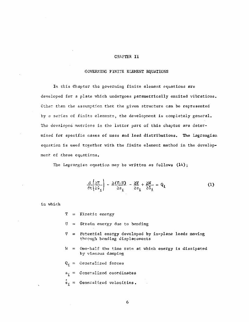
The Lagnnghn equation mil!y be written as follows (14);
in which
T = Kinetic energy
U = Strain energy due to bending
V = Potenti.al ffnergy developed by in-plane loads moving through bending displacements
W = One=half the time rate at which energy is dissipated by v:i.scous damping
Qi = Generalized forces
Si = Generalized coordinates
Si ::;; Gene,rdized velocities •
6
(1)

7
Let a small element of fi.nite dimensions be isohted from a plate
and the lateral displar.ements of t~e element be represented as
(2)
in which w(x,y) is a function of x and y only, and R(t) is a time
functi0n. Here the middle surface ef the plate is taken as lying in
the x-y plane and w is measured downward from thi~ plane. Further it
is assumed t~at the functien w(x»y) can be represented as a linear
•
A n
To determine the constants {A}, then nodal displacements ef the finite
plate element~ {v1R(t)}, ~re chosen as generalized displacements. !hat
is to say
(4)
These node displacements c~n be expressed as follows,
{5)
The matrix [BJ is obtained by evaluating the matrix (fn(x,y)] and its
derivatives at the nade points. Solving for the copstants, {A}, from
Eq. (5) yields

8
(6)
.and by substitution into Eq. (3) the displacement function can be ex-
pressed as
Because the matrices [BJ and lviR(t)} are not functions of x and y,
the derivatives of w(x,y,t) may be formed as follows;
~= of (x~y) -1 n [BJ [viR(t)}
(IX c)X . " of (x,y)
~= -1 n [B] {v1R(t)} oy oY
o~ == ·l §R(t) ot [fn(x,y)][BJ {vi dt } •
With the above information expressing the displacements of the plate
element in terms of nod,il er generalized displacements, the terms in
the L,ag:rangian equati@n cai1. be ev.lilluated in a finite element f@rm.
2.1 Kinetic Energy
(8)
The kinetic energy fer an infinitesimal area of the plate element
is
in which pis the mass of the plate for a unit surface area. If this
expression is integrated over the entire surface of the plate element,
the total kinetic energy fo,r the element becomes,

9
(10)
Substitutiag from Eq. (8) into Eq. (10),
(11)
The squaring of .the term in the brackets can be accomplished by
multiplying the expression by its transpose.
This expresses the total kinetic energy of the plate element in terms
of the generalized nodal displacements.
Now the necessary operations are performed on the kinetic energy
term fqr substitution into the Lagrangian eq~ation. Tb.e first term of
Eq. (1) t:hen becomes,
_g_(.Q,.i-) = ...$!_( oT -) = [[Bf1]T [fJ(f (x,y)]T dt os. dt dR(t) n
1 o (v ) · i dt
T . The [[BJ-l] , [B]-l
2 and {v1d R(i)} matrices can be factored out as
dt shown since they are independent of the variables x and y. Using a
more concise natation
d(oT ) dt ~-
1. (i=l,2,3--n)
(13)
(14)

10
in whfoh
The matrix [m] is designated as the elemental mass matrix and hereafter
is referred to ~s such.
'!'he remaining term involving the kinetic energy is
oT .: o, osi -
(16)
since the kinetic energy function is independent 0f the variables s1•
2.2 Strain Energy
The strain energy for the entire area of the plate element is
Sii 2 2 2 2 ( 2 )2 J Dowow owow ow U = 2 ~~·2(1-v)[ ~ ::--I- ---- ] dxdy. ox oy ox oy oxoy
(17)
This can be represented in matrix f0rm as
(18)
in wb.ich 2 :a:: l \I 0 ox" 2
{c} = ~ , and [DJ ::::; v 1 0
~ 0 0 2 (1-v) • oxoy
Matrix (C} can be expressed in terms of the generalized displacements
as
(19)

11
in which
2 o f 1 (x)y) 2
a f2 (X»Y> 2 o fn(x,y) --
ox2 ox2 ox2
~2£1 <:x~y) 2 2
o £2 (x,y) o fn (x,y) [E] =
oY2 oy2 oY2
2 O fl(XvY)
2 o £2 (x,y) 2 o fn(x,y)
oxoy oxoy oxoy
Substituti.ng into the strain energy expression the strain energy
becomes,
T I'fDL }T[ -lJ T -1 U = J2lviR(t) [BJ [E] [D][E][B] lv1R(t)}dxdy. (20)
Now the operations indicated by Eq. (1) are performed
(21)
or
(22)
in which
(23)
By definition the [k] matrix is the stiffness matrix for the element.
2.3 Work Done B~ In~Plane Load!
The work done by the parsmetric or in-plane loads when they move
through the bending displacements is
(24)

12
This expression may be represented in matrix form as follows;
(25)
in which.
and
(_
L~y ~yj [NJ= • Ny
The matrix [IGJ is as follows;
of1 (x,y) of2 (x,y) ofn (x,y)
ox ox ox [GJ =
of1(x,y) of2 (x,y) of (x,y) n
oY oY oY
Substituting these expressions into Eq. (25) the potential energy term
becomes,
T
V = .\fJ{viR(t)} T[[Bf1] [G]T[NJ[GJ[Bf1{v1R(t)}dxdy, (26)
which when differentiated with respect to s1 , yields
(27)
O!'
"ii!- = [S](v.R(t)} osi 1
(28)

13
in which
[SJ
Matrix [SJ is hereafter referred to as the elemental stability matrix.
2.4 Damping .and ~~c Feund.ation
To include the effect of viscous damping, the expression for the
rate at which ene~gy is dissipated due to the damping forces must be
calculated. This is done by multiplying the damping force by the
velocity. One,cJ:uilf the !'.l'.lte at which damping energy is expended is
2 dW ::: \ (2c) ( ~:} dxdy, (29)
where 2c is the damping coefficient, and here it is assumed to be con-
st.ant over the pl~te element. Integrating over the area of the plate
element
W == JJ(c)[~(x.y,t2]2dxdy. at · · (30)
Comparing Eq. (30) with the e~~pression for kinetic energy, Eq. (10), it
can be seen that when the mass (p) and damping coeffici.~mt (c) are both
constant over the elementvs area the integrals to be evaluated are
ident:i,cal except for these constant terms. The damping term in the
Lagrangian equ.ation is rwt ~ however, differentiated with respect to
time. By comparison with the development for the kinetic energy the
damping term is
(31)
In writing this expression the mass has been assumed to be constant
over the ent:i:re plate element.

14
The effect of an elastic foundation can be taken into account by
finding the work done by the elastic foundation forces and differentiat-
ing the work with respect to the generalized coordinates. Thus,
where q is the spring constant for the elastic feundation per unit area
of plate surface. Here again, as for damping, by comparing this expres-
sion with the kinetic energy development it is obvious that
(33)
In the above expression i.t is assumed that both the foundation modulus
and the mass a:re const.int over a given plate element.
2. 5 Governing Eguati.£B.!
By using Eqs. (14), (16), (22), (28), (31), and (33) in conjunction
with Eq. (1), the governing equations for a plate can now be generated
for the various cases of loading and motion. Several cases are listed
below. The m@trices in these equations denoted by the capital letters
are matrices for a complete plate corresponding to the elemental
matrices with, the same small letters. For example the matrix [KJ in
Eq. (34) is the structural stiffness matrix. The details involved in
constructing these structural matrices are discussed in Chapter IV.
1. Static deflections of a plate due to transverse loading
[KJtv} == [Q} (34)

[M]{v,g:!Ul} + [K]t_vR(t)} = 0 dt2
and for harmonic motion of the form
v.R(t) = A. sin wt l l
the frequency determinant becomes
3. Static buckling
[[K] • [sJ]{v} = 0
or
From this determinant static buckling loads can be determined.
4. Deflections of a plate on an elastic foundatian
[KJ{_v} + .9. (M]{v} = {Q} p
5. Dynamic Stabili.ty
6, Dynamic Stability including damping
The equations for other combinations of facto~s affecting the plate
response can be formed in a similar manner.
15
(35)
(36)
(37)
(38)

16
In the expressions for the mass, stiffness, and stability matrices,
once the displacement function w(x,y) is known the matrices [f0(x,y)J,
[E] and [GJ can be determined, and the integrals can be evaluated for
particular cases.
Assume the displacement function for the rectangular plate element
shown in Figure (1) takes the form,
b
w
Figure 1. Finite Element With Generalized Coordinates

17
or in matrix form.
Although other displacement functions could be used, the one chosen here
has certain advantages. Eq. (40) is the highest order polynomial which
identically satisfies the homogeneous plate equation
t;4w(x,y) = O.
If the generalized coordinates are chosen as the ones shown in Figure
(l)i then Eq. (5) can be e~pressed as shown in Figure (2). When the
various elements are assembled together to represent a plate, the de-
flections and slopes are completely compatible only at the node points.
Compatibility is also maintained along the connecting boundaries in
the direction 0f the bouadaries, whereas in general slopes are slightly
discontinuous across the boundaries.
Matrices [E] and[~] in Eqs. (20) and (26) may now be constructed
using the chosen displacement function. These matrices are shown in
Figure (3). The elemental mass, stiffness, and stability matrices, [m],
[k] and [SJ, are developed by substitutinginto Eqs. (15), (23), and

{v} = [BJ { A }
wl l 1: 0 0 0 0 0 0 0 0 0 0 ol I Al
wlx l 0 0 0 0 0 0 0 0 0 0 I I A2
1 ·~ t')' I a
0 0 1 0 0 0 0 0 0 0 0 0 I I A3 w ly b
.. 7 l ,
0 l 0 0 1 0 0 0 0 0 I I A4 le. 2: J!.
0 l 0 2
0 0 3
0 0 0 0 0 A w2x - -a a a 5
0 0 l 0
1 0 0
l 0 0.
1 0 A6 w2y = b b b b
....
w3 l l 1 1 l 1 l l l l 1 1 I I A7
1 2 ' 3 2 1 l l 0 0
.t. 0 0 A8 w3x - - - - - -
a a a a a a a -a
w3y 0 0 1 0 1 £ 0 1 2 l 1 l A b b b b b b b b 9
W4 l 0 1 0 0 1 0 0 0 l 0 0 A 10
"'4x I I 0 1 0 0 1 0 0 0 l 0 0 1 All a a a a
w4yj Lo 0 1 0 0 2 0 0 0 l 0 0 I I \2 bi b b
Figure 2. Generalized Coordinates,Function of Constants
!-' (JO

0 0 0 .l.. 0 0 6x ~ 0 0 6xy -0 rl- 3
a2b .?o a
[EJ = lo 0 0 0 0 2 0 0 2.x ll 0 6xJ b2 ~ b3 ~b ab
.1... 2.x 1L 3x2 2 0 0 0 0 0 0 0 ll_
ab a2b ab2 a3b ab3
! 2x 2
2iy 2 2 J
0 0 :L 0 2x -1y 0 ~ _.L_
2 T ~?b ab3 [G] I
a a ab a a b ab =
l h 2 2xy 3y2 x3 3xv2
0 0 0 x
0 x - a2b b2 ab2 3 a3b ab3 b ab b
Figure, 3. [E] and [ G J Matrices
t;

20
(28) :respectively. Ms!:!tric:es [m] imd [k] are sh®wn in Figures (4) and
(5). In the mass m.atrix shewn the mass per unit area is taken as con~
st.lint. The stability matrix is separated int0 three parts reflecting
indivi.dually the :!.nfh11ence @f Nx, Ny' ap.d Nxy• These ni.atrices are
shown in Figures (6) through (8) .. for load distributions which are con ..
stant across an edge of the plate. All of the elemental matrices in
Figures (4) through (8) have been non~dimensionalized, and the gener~
alized displacements and forces as a result are,
wl Fl
awlx M I . lx a
bw1 -Y Mly/b
w F '.I 2 "" aw,, ... x M2x/a
bw2 y M2y/b
{v} = w 3
{q} = F3
,!!lW3 . JI: M3x/a
b>s~:1" M3y/b
w Li F4
aw 4x M4x/a
bv,J 4y M4y/b

3454 461 461 J.226 -274 199 394 -116
80 63 274 - 60 42 116 ... 30
80 199 • 42 40 116 .. 28
3454 -461 461 1226 .. 119
80 -63 -199 40
[m] = p 80 274 - 42 _ p ab p = 25,200 3454 -461
80
{Symmetrical)
Figure 4. Elemental Mas~ Matrix
-116 1226
~ 28 199
.. 30 274
-274 394
42 -116
- 60 116
-461 1226
63 -274
80 -199
3454
199
40
42
116
-30
28
274
- 60
- 42
461
80
-274
.. 42
• 60
-116
28
- 30
el99
42
40
-461
- 63
80
N ....
-4P + 4P•l 2P·l + l + !!.II 2P +].+!!.II 2P • 4p·l 2P·l + .IL P·i·ti ·l p·l • .e.... ·2.P • 2P 5 5 5 5 10 10
+li.!!.11 . !i + !!.II + l!t.. !!.II 5 5 .s 5 5 5
ip·l + li ·2P·l • .IL 1.p·l • .e... -1 + v 0 .p·l + .IL ;- +fa 3 15 10 3 30 10
ip +li . 1 !!.II 0 tp • H ·P + fu 3 15 p • 5. 5 0
4P + 4P·l -2P· 1 • l 2.P + l +!!.II ·4P + 2.P·l ·l l ·P + -
5 5 5 +l!i.!!.11 • !!.II • .!i + !!.II + !!.II
5 5 5 5 5 5
ip"1 + li • v .p·l + l 1i,·l • li 3 15 5 3 15
+~ 5
[k] = * p = (!./ b !P +H ·2.P • fu 0
4P + 4p·l ·l l ·2.P • -
5 ~ = 2 (l • v) +.!i.!!.11 • !!.II
5 5 5
4 -1 ~ 3p + 15
(Symmetrical)
-
Figure S. Elemental Stiffness Matrix
p • .e... 10
.4p + 2P·l
.li+!!.11 5 5
p·l • l . !!.II
0 5 5
t + to ·21' • to-·l
2.P +L ·2P • 2.P 10
+l!i.!!.11 5 5·
0 ·l • .IL p 10
tp. to ·P + fu
·2P • l 2.P • 4p·l . 5
• ~ +!!.II -~ 5 5 5
\I 2P" 1 + L
. 10
!!.p + li .p + !. + ~ 3 15 . 5 5
4P + 4p·l·
+li-~ 5 5
p·l • l . !!.II 5 5
fr·l • ¥s
0
.p·> + fu
p·l .IL T + 30
0
·2.P·l • JL 10
. 1P.r. L 3 30
0
2.P·l + l 5
+ !!.II 5
!!_p·l + li 3 15
2P +JL 10
0
Ip· to p • .IL
10
0
I+ to .p·+ l
5 + !!.II
5
0
1.p. li 3 15
·2P • 1 5
• !!.II 5
• \I
ip + li 3 15
-
-
N N

1104 84 132 =1104 84 =132 =408 42 78
112 0 = 84 =28 0 = 42 =14 0
:24 = 132 0 = 24 - 78 0 18
1104 -84 132 408 =42 = 78
112 0 - 42 56 0 I
N
[sJ---2... I 24 78 0 = 18 x . .2520k
k == (.!) b 1104 =84 -132
I Q . I 112 0
x 24
bl Nx=1 rNx (Symmetrical)
I 1-tY
Figure 6. Elemental Stability Matrix for N x
408 42
42 56
78 0
-408 =42
42 -14
- 78 0
-1104 -84
84 -28
132 0
1104 84
112
= 78
0
- 18
78
0
18
132
0
- 24
-132
0
24
N w

1104 132 84 408 - 78 42 - 408 78 42 -1104 -132 84
24 0 78 - 18 0 - 78 18 0 - 132 .. 24 0
112 42 0 56 .. 42 0 -14 .. 84 0 -28
U04 -132 84 -1104 132 84 - 408 ... 78 42 a k = (b)
24 0 132 .. 24 0 78 18 0 I
N k
[sy] = mo I 112 - 84 0 -28 - 42 0 -14
,- Q -1 1104 -132 -84 408 78 -42
Ny 24 0 - 78 - 18 0
' 1 i l t x
E: 112 - 42 0 56
I 1104 132 -84
I I (Syrmnetrical) 24 0
ty Ny 112
Figure 7. Elemental Stability Matrix for N y
~

1260 0 0 0 0 -252 -1260 252 252 0 -252 0
0 35 0 0 - 35 - 252 42 35 252 0 - 35
0 252 -35 0 • 252 35 42 0 - 35 0
-1260 0 0 0 -252 0 1260 252 -252
0 35 252 0 -35 - 252 - 42 35
[ N 8xy] = 25~& I 0 0 - 35 0 252 35 . - 42
N 1260 O· 0 0 0 252 xy .-&-....._........_....._ .--.
~ ) x 0 35 0 0 - 35 ~ t ~ ~ 0 - 252 - 35 0
~ ~ -1260 0 0 ~ ~ [-~-~N,y (Symmetrical) 0 35
0
Figure 8. Elemental Stability Matrix for Nxy
~

CHAPTER III
BOUNDARIES OF STABILITY FOR LINEAR EQUATIONS
WITH PERIODIC COEFFICIENTS
Both Eq. (38) and the more general one, Eq. (39), 0£ the previous
chapter represent a system of second erder differential equations with
periodic coeffici~nts. Equati@ns of this type are known as Mathieu
Hill equations, and the criteria for stability of their solutions have
been well established by several investigators such as Cesari (15),
and Chetayev (16). The solutions may be greuped into two classes; one
class is stable and bounded and the other is unstable and unbounded.
The stability er instability of the solutions corresponds to the
stability or instability of the structural system at hand. The spectrum
of values of the parameters yielding stable solutions farm the so
called regions of stability, while those yielding unstable solutions
form the regions of instability. It is clear that the analysis of
structures for dynamic instability reduces to the finding of the
boundaries separating the regions of stability from the regions of
instability. It is the purpose of this chaptei to review the basic
principles of the theory of these equations and to formulate the neces
sary conditions for the determination of the above mentioned boundaries
in a form amenable to the finite element method.
3.1 Behavior of Solutions
First consider a system of equations which has the same form as
26
27
the system given by Eq. (38).
2 [HJ{d iJ+ [CJJ - a.[LJ - ~R(t)[N.J]Lf} = 0
dt (41)
in which [HJ, [JJ, [LJ and [NJ are matrices containing constant terms
and R(t) is a continuous periodic function with a period T,
R(t+T) = R(t). (42)
For convenience and te give greater symmetry to the solution of these
equati®ns~ this sytem of (n) second order equations is replaced by an
equivalent system of (2n) first order equations by making appropriate
variable changes.
Rewriting Eq. (41) as
in which
ifi ?, ~·+L dt k=l
and introducing the new variables
x = f. (j = 1, 2, - - - - n) j J
= df i-n xj dt
(j = n+l, n+2, ---- 2n)
the resulting system of (2n) equations becomes
dx i -=
dt
dx _!, + dt
(i = 1, 2 9 ---- n)
n
[ ( i = n+l, n+2, ---- 2n).
k=l
(43)
(44)
(45)

28
In matrix notation
· &hl + [R(t)J{x} = o. dt
(46)
The structure of [R(t)] will be as follows:
[R(t)] =
It is clear from Eq. {42), that matrix [R(t)J is periodic with a period
T.
The solution of equations ot the form given in Eq. (45) is not
always possible, but fortunately the complete solution is not needed to
determine the spectrum of the stability or instability of the equations
(15, 16). The investigation of these equations is facilitated by the
fact that with the substitution
t + T = t
the form of the equations remain unchanged. Applying this substitution
an unlimited number of times to the solutions {x81, which are assumed
to be known for the time interval (O,T), the behavior of the solution
can be determined for an unlimited variation of the variable t (16).
Assume that the (2n) linearly independent solutions of Eq. (45)
are known within the interval t = (O,T)1
Or writing in matrix form

29
xu (t) x12 (t) ••• xl, 2n (t)
x21(t) X22(t) ••• x2,2n(t) [X(t)] = '
(47) • • •
•
x2n,1 (t) x2n,2(t) ••• x2n,2n(t)
where the first subscript represents the number of the function and the
second subscript represe~ts the number •f solution. From the properties
of linear equations wit~ periodic coefficients with the invariant
substitution t + T = t, the functions
(48)
also represent a set of solutions, and they can be expressed as a
linear combination of the independent solutions (15, 16).
[X(t+T)] = [AJ[X(t)] (49)
From the selected independent selutions a similar set of solutions is
constructed by a linear transformation with constant coefficients.
{ xs} = { b1x1 (t) + ....... + b2 x2 (t)} ,s n n,s (SO)
The constantsD bi' are chosen.such that this set of solutions has the
fundamental property,
(51)
To determine the constants h1 substitute from Eqs. (49) and (50) inte
Eq. (51),

30
b [a x (t) +----a x (t)] = n 2n,l ls 2n,2n 2n,s
( s = 1 2 ---~ 2n) ' '
These relationships should be satisfied regardless of the value of the
variable t, therefore, identical coefficients can be equated.
[AJlb}=P[b} (52)
This system af linear algebraic equations has a non-trivial solution if
the determinant of the coefficients vanish.
(53)
The values p1, p2 , -- pn which satisfy the relationship given in Eq.
(53) are then connected with the fundamental particular solutions. For
this particular set of solutions Eq. (49) becomes
[X(t+T)] = [DI.AG Pk][X(t)].
Or in vector notation
(54)
Eq. (54) can be written with the diagonal matrix cf p's only if the
roots of the characteristic Eq. (53) are distinct, which permits [A]
to be reduced to the diagon<;iil form. In the case where there are
multiple roots of the characteristic equation, [A] can be reduced to
the Jordan normal form~ and the fonn of the solutions depends upon the

structure of the elementary divisors (p - pi) of the characteristic
equation. In either case there is at least one solution of the form
The fundamental form of a continuous, single valued function which
satisfies this relationship is
31
{ i : (trt)lnp } x (t)J = LZ (t)e. k
k k (55)
waere { Zk (t)} is a periodic v~ctor with. a period (Tl~
3.2 Roots of Characteristic Equation
It can be shown that the characteristic·equation formed from Eq.
(53) is a reciprocal equation. Tkat is to say the equation
+ -----
has root, pk and also 1/pk. The proof of this is given here for the
case when R(t) i.s an even functien (1). Tb.is cue is the cme of most
importance to the work presented :i.n this thesis. For an even valued
function
R(t) = R(·t) •
Since the form of the differential equation system is unchanged when
(-t) is substituted for (t), and since
t -lnp {x(t)} =lZ(t)e T J
is a solution cf the system of equations, then

32
is .also one of the solutions of the system. Therefore, 1/p is alse 0.ne
of the characteristic reots.
3.3 Regions ef Stability and Instability
The system under consideration has solutions, other than the
trivial solution, of the form given in Eq. (55). The characteristic
exponent in this relationship is
It is clear that if all the characteristic expenents have negative real
parts the solutions will damp out with time increasing. But if among
the ch.art'lcterhtic expenents there is one with a positive real part the
solutions will be unbounded or unstable. Censidering that
it can be seem that if any root of the characteristic equ•tion has an
absolute value greater than unity instability occurs.
Now consider the fact that if pk is a root of tl:ie characteristic
equation then lfpk is alsG a root of the equation. The solutions
corresponding to these two roots are
(56)
If pk _is any real number different from ± 1, then one of tlie solutians
above will increase unboundedly with time. Therefore, w~en any one of
the roots of the characteristic equation is real and different frem ± l
instability will occur. If the coefficients of the system are varied
such that the roots p = 1 or p = ·1 are obtained then the solution k k
will be periodic since the function{Z(t)}is periodic. In the case
where p = 1 k
i[lnjll + i(O)]} lx (t)} ={Z (t)e =lz (t)} k k k •
33
The solution has a period of T since"i,Zk(t)}has a period of T. For tb.e
case when 'pk= ·1
/)
ln pk= lnll I+ i"l'r
s i1f {xk(t)} = {zk(t)eT } •
This solution is periodic •nd has a period equal to 2T. With a further
variation of the coefficients of the system the pairs of roots of the
characteristic equation will become complex conjugates,
pk== m + ih
Pn+k = m • ih
Since it bas been shown that pk and 1/pk are roots. taen in this case
PkPn+k = 1. The absolute value ef each ctmplex root is therefore equal
to unity, amd the region of stability or beunded solutions is tbe
region of complex reots.
lt follows from the preceding treatment that the boun.daries
between stability and instability are periodic solutions tdtn periods
oft or 2T. Two solutions of the same period confine the region of
instability and two solutions with different periods confine the
region of stability. this follows from the fact that the root p. a O k
cannot lie in the interval between pk= land pk; ·l because of the
non~singularity of the transformation given in Eq. (49). Therefore;

34
the problem of determining the regions of instability of Eq. (41) is
merely a problem of finding periodic solutions of periods Tor 2T of
these equations (1) •
. ) .4 Boundary Frequencies for Instability
As was shown in the preceding sections, the finding of regions of
instability or boundaries for instability reduces to the finding of
periodic solutions of period Tor 2T for Eq. (41). Here the periodic
function R(t) will be taken as
R(t) = cos (9t)
and Eq. (41) becomes
2 [HJ{~}+ [[JJ - a.[LJ - ~[NJ cos(9t)]{f} = 0. (57)
dt
The solution of Eq. (57) is sought in the form of the convergent
trignemetric series,
{f (t)J = L { akJ sin k~t + {bkJ cos k:t
k=l,3,5
where lsk~ and {bkJ are time independent vectors. Substituting Eq.
(58) into Eq. (57) the following matrix equations are obtained;
2 [CJ] - a.[LJ + ~~[NJ - !z:-(HJ]{a1} - ~~[NJla3} = 0
[[JJ .. a,[LJ .. k:92[HJ][ak} .. l.ia[NJ[{ak .. 21 +{sk+23] =O
(k = 3,5,7 ....... )
(58)

and
[[JJ • a.[L] • \~[NJ • f[HJ]{b1} • ,\~[B]lb3} = 0
2 2 [[J] • a.[L] • k 4g [HJ] ibk} - \~[NJ [{bk-21 + lbk+2JJ = 0
(k = 3,5,7 ----)
35
The condition for the existence of solutions with a period 4 Tr /Q is that ·
the determinant of the coefficients of [ak} and{_bkl must vanish. In
this case the equations for {ak} and {bk} ~re separable and the two con
ditiens are combined with the (±) sign.
2 [JJ•a.[L]~~[N]-~ [HJ -\~[NJ 0 ..
2 -\~[NJ [J J·a.[L ]-filL[H]
4 -~~[NJ
2 = 0 0 ·t~[NJ [JJ•a.[LJ·2!9 [HJ •
(59)
By substitution of tae series
lf(t)} = ~{b0} + L { ak} sin~+\ bk~ cos ~ • (60)
k=2,4,6
the followins coruUtiens are found for the existence of solutions with
a period 2'tr)'9;

36
2 [J]~et[L]·Q [HJ -\[,[NJ 0
-~[,[NJ [J)·et[L]·492[H] -~[,[NJ •
2 = 0 (61) 0 -.~[,[NJ [J]·et[L]•169 [HJ
•
and
[J]·a.[L] ·[,[NJ 0 •
-\~[NJ [JJ•a[LJ·92[H] ·\~[NJ
[J ]·et[L]•492[H] = 0 • (62)
0 ·\r,[N]
• • •
All three of the relationships given in Eqs. (59), (61), and (62)
are infinite determinants. Fer the case where the period is 41f/9, the
first term of the determinant taken alone yields values of Q which give
the zeroes of the infinite determin1nt with reasonable accuracy (1).
Therefore
[JJ .. o.[LJ ± ·~[NJ .. f[H] I = 0 • (63)
Using only this first term is equivllent to 1asuming that the function
{.f(t)} can be adequately represented as follows;
Similar approximations can be made for the case where the period is

37
3.5 Equation With Damping Terms
In this section equations which contain terms involving the first
derivative are considered. Con,ider tb.e following matrix equation;
[HJ[g} + 2g[HJ[~} + [BJ{£} = 0 dt dt
(64)
where the matrix.[BJ is periClldic with a period T, [H.J is a constant
matrix and g is a constant. Assume that Eq. (64) has a solution of the
same ferm. as the analogous single equation with a damping term. That is
Differentiating
When these expressiens are. substituted into the d:lffetential Eq~ (64) t
the terms involving the f:l.rst derivative vanish and 'the resulting
equatien is as follows,
Since e·gt is a scalar factor it can be factored out of the equation
(65)
The term e·gt does not v1nish., therefore, the term in the bracket in
the above expression must vanish. The same arguments can be used for
finding the regions of stability of Eq, (65) as was done for Eq. (41) 1
since tbe term in brackets,

38
[H]{_u11 (t)} + [[BJ • g2[HJ]{u(t)} = 0
has exactly the same form as Eq, (41).
If the matrix [BJ is taken as
[BJ= [JJ - a[LJ - ~ cos(Qt)[NJ
then the condition for existence of solutions with a period 41f{Q is as
follows;
2 [J] • ~[LJ +~~[NJ· -\-[HJ
Qg[HJ
·9g[HJ
2 [JJ • a[L] ·~~[NJ· ~[HJ
= 0 (66)
The determinant shown is the central elements from the infinite deter-
minant which is obtained.
3.6 Physical Considerations
The farm of th.e equations discussed in this Chapter are identical
tQ Eqs. (38) and (39) in Cb.apter II. The fact th.at the boundaries
between stable and unstable salutions are periodic solutians Cl)f the
differential equatien is net surprising when the physical system is
visualized. Basically there are three types of vibrations that the
plate can perform: (1) vibrations which are damped out with time, (2)
vibrations which are perif)dic, and (3) vibrations whose amplitudes
become unbounded as tiJne increases. Periodic solutiens, by their
nature, form the boundary between bounded and unbounded solutions.
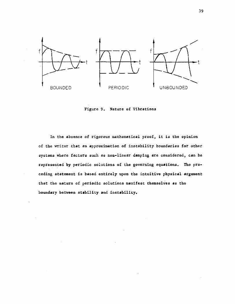
The. three types of vibr1tions are shown in Figure (9).
39
---~ .............. BOUNDED PERIODIC UNBOUNDED
Figure 9. Nature of Vibrations
In the absence of rigorous mathematical proof, it is the opinion
of the writer that aa approximation of instability boundaries fer other
systems where facters such u nom•linear damping are censidered, can be
represented 'by periodic solutions of the governing equatiens. The pre-
ceding statement is based entirely upon the in,tuitive physical argument
th.at the nature ef periedic solutions mam.ifest themselves as the
boundary between stability and instability.

CHAPTER IV
SOLUTION FOR THE REGIONS OF
DYNAMIC INSTABILITY
The general preblem which is solved in this thesis is illustrated
in Figure (10). Tlile beundaries ef dynamic instability are found for
this problem fer different ratios of the leads N, N, and N , differ-x y xy
ent aspect ratios, and it is Jelved bath with and without including the
effects ef an elastic foundation and visceus damping. The problem is
alse solved with varieus boundary conditions. The ease with which the
different bouudary conditiens are handled is the primary advantage ef
the finite element method. The finite element grid size used te selve
a particular problem is variable depending upon the amount of computer
time and storage space available. The number ef generalized coordinates
er degrees of freedom for a given p:re'blem will depend upen the grid
size selected. Since each node point can have three generalized
displacements (one translation a]l).d two rotatiens), the total number of
degrees of freedom for the plate will be 3 (m+l) (n+l) minus the number
of constraints imposed by the boundary conditions, where mis the number
of plate divisions in the·x-direction ~nd n is the number of divisions
in ~he y·dire~tion. Another factor which influences the selection of a
grid size is that the number of degrees of freedem ·~~owed must be
sufficient te represent adequately the mode shapes of the plate.
40

......... ...... <D U) 0 u
)( -z +
)(
0 z
I
-,. ..
• --
Ny= Noy+ Nty Cos (8t)
-I
( e ) ( d)
I n
( f ) (a)
Q) ® rsz:: m
@ @
~ . ~ --- ........ I I
( c ) . i .
( b ) ' -~
Ir
II )( -+ ( g) ( h) ( i )
z A
I . .
- . I
~ I
-+.. \ I I . \
. . - - . ~~)
= + = Ny N0y N ty Cos( 91) i y Nxy Noxy t Ntxy Cos( 91)
Figure 10. General Problem
41
-...... <D ....__. U)
0 u
)( ..... z + )( 0 z
II )(
z --x

42
4.1 Formulation of the Structural Matrices
The first step in applying the finite element method to finding
the regions of dynamic instability is to divide the plate into finite
plate elements and form the tatal structural matrices corresponding to
the elemental matrices developed in Chapter II. To accomplish this,
the effects of all plate elements joining together at a node point are
added together. Fer example, consider elements I, II, III, and IV
which have the common node point (a) as shown in Figure (10). Let the
node points for each individual element be numbered as the ones shown
on element III. Then the elemental matrices shown in Figures (4)
through (8) (the example used here is the stiffness matrix) may be
partitioned into (3x3) matrices as follows;
k12i I k22i I k32i I k42i
[k] = (67) -- -- -- -- ---kl3i k23i k331 I k43i
Noting that each term in the Lagrangian equation (Eq. (1)) has the
units of generalized force, then the structural m•trices may be formed
by adding the forces at each node point. The subscripts used fer the
sub-matrices in Eq. (67) have the follewing me11ning; the sub-matrix
k1 is the force at node point m caused by the deformations at node mn
point 1 for the plate element n. The structural stiffness matrix will
have the following form

43
Ka CKi,a CKca .. c~a ,.
CKab CKc'b .. . . • • •
[K) • • (68) =
•
• • • •
• Kn
In each line of the above matrix there is a carry~over term, CKji• fGr
every node point adjacent te node point i. The stiffness, Ki' and the
carry-over stiffness, CKji' matrices for an arbitrary point (a) are
•
The structural mass and stability matrices are formed in exactly the
same manner as the stiffness matrix.
4.2 Boundary Conditions
After the formation of the structural matrices the necessary
boundary conditions or constraint conditions must be applied. Since
there are three pessible degrees of freedom at any node point there are

44
three possible constraints which may be applied either singly or in any
combinatfon. The possible displacement type constraints far node i
are,
w. = 0 l.
w = 0 iy
The common types of boundary conditions for plates are as follows;
l, Rigid column support
w = 0
w == 0 x
w =0 y
2. Pinned column support
w = 0
M = 0 x
M = 0 y
3. Simple edge
at all node points along the edge
w = 0
wt = 0 (slope along the edge)
M = 0 n
4. Chmped edge
at all node points along the edge
w = 0
w = t
0 (slope along the edge)
w = 0 n
(slope normal to the edge)
The constraint conditions are applied to the structural matrices by

45
deleting the corresponding rows and columns. If n is the number of
node points and r is the number of constraints, the final size of the
structural matrices will be (3n - r).
4.3 Solution
The governing equations for the plate, Eqs. (38) and (39), can now
be formed. Let the in-plane loads be expressed as
N = N0 + Nt cos(9t) = aN + bNt cos(9t) x x x s
NY= Noy+ Nty cos(Qt) = cN8 + dNt cos(Qt)
N = N0 + Nt cos(Qt) = eN + fNt cos(9t) xy xy xy s ·
The loads are represented in this manner so tha.t each term contains the
common factors Ns and Nt• Substituting into Eq. (38) and factoring out
the commcn terms in each matrix the following expression is obtained;
pab [MJ{U} + Jl..[K] - ......!...[s ] - -Les ]cos (Qt) l v J = o. 2- [ a.N * _ !,N * _ ~ _
25,200 dt2 ab 2520 8 2520 t
in which
N8 = al\* Nt = !,Ni*
[s8 J = a[sxJ + c[syJ + e[SxyJ [stJ = b[sxJ + d[i1J + £[ixyJ
(69)
N1*•s are the static buckling loads which are determined as the eigen
values of the determinant
(70)

46
(69) reflects the influence of the static components of the loads while
the term ~N1*[St] reflects the influence of the pulsating components of
the loads. By comparison of terms in Eqs. (38) and (41) the equation
which gives the boundaries of dynamic instability (Eq. (63)) is found
to be
::; 2 lL[K] - ~Ni*[s J ± ~Ni* [S] - pab(ew1) [M] = 0 (71) ab 2520 s 2(2520) t 4(25,200)
in which
The wi's are the natural frequencies of the system determined from
Eq. (35),
2 ~a~b[KJ - pabw lM] = 0
25,200 (72)
In the same manner, the characteristic determinant for determin•
ing the regions of instability, when the effects of viscous damping
(Eq. (66)) is considered, becomes
(ew)ca~[M] 25,200
• (~w)cab[MJ 25,200
= 0
:(73)
If the effect of an elastic foundation is considered the only change in
Eqs. (70) through (73) is that the term

47
lL[K] ab
is replaced by
J2.. , K + 98 · M • .. ~ 2b2 J ah· [] 25,200(D)[]

CHAPTER V
DISCUSSION OF RESULTS
5.1 Interpretation of Results
A program for the IBM 7040 electronic digital computer was written
to solve Eqs. (70) through (73) for the natural frequencies, static
buckling loads, and regions of dynamic instability for several plates.
The results are shown in a series of figures and tables, and are
expressed non-dimensionally in terms of the parameters~,~ and 9fw.
As can be seen in Chapter IV the parameter~ is the percentage of the
static buckling load which is applied statically,~ is the percentage
of the static buckling load which is the amplitude of the pulsating
load, and 9fw is the ratio of the frequency of the pulsating load to
the natural frequency of transverse vibration of the plate. In all of
the examples both the static and the pulsating components of the loads
Nx, Ny, and Nxy were applied proportionally. The static and the pul
sating components of the loads were applied independently, but each
type of leading was varied in the same proport~ons as the ones used to
determine static buckling loads for a particular example. That is; if
in determining the static buckling loads, N1*, the loading is applied
as~= N, N7 = .SN, and ~y = .SN, then the static and pulsatittg com
ponents of the load used in determining the regions of instability
are varied with these same proportions. This type of loading allows
the results to be presented in a uniform non~dimensional form. The
48

49
method which has been presented is not, however, restricted to this
type of loading. The subscript i which appears with the parameters a,
13 and 9fw, on some of the figures depicting the results, indicates that
th th the results are for the i natural frequency and i · buckling load,
each of which is ranked numerically. For example, when considering the
region of dynamic instability corresponding to the 1th natural fre-
quency (G1rw.) the load axis is non-dimensionalized with respect to the . 1
th th i buckling load, with a and~ being percentages of the i buckling
load. Also shewn on these figures are the constants necessary to cal-
culate the natural frequencies and buckling loads for several of the
lower modes once the physical properties 0f the plates are specified.
With this information in addition to the curves, design loads and fre-
quencies can be specified. In addition to the figures which show the
regions of instability the mode shapes for free vibration and static
buckling for some of the examples are shown. As is pointed out later,
these mode shapes are helpful in interpreting the results which are
obtained.
5.2 ,I'.lates Without Dam.pins
The first series of examples which was solved is as follows;
Lo$_ding
s.s Ny em N, Nxy = 0
s.s s.s N = •05N. ~v 1z .SN
y "
s.s Ny= 01 Nxy = .SN
Nx = O, Ny=), Nxy = N
Nx = .lN, Ny= .lN, Nxy = N

5()
afb = 1.5 (*)N = N, N = N, N = 0 x y xy
(*)Nx = N, N = .SN, Nxy = .SN y
N = N, N = 0, N = .SN x y xy
c afb = 1.0 (*)Nx = N, N = N, y Nxy = 0
N = N, N = .SN, N = .SN c c x y xy
N = N, N = o, Nxy = .SN x y c
(*)N = N, afb = l.S N = N, N = 0 x y xy
N = N, N = .SN, Nxy = .SN x y
Nx = N, Ny= O, ~y = .SN
afb = 1.0 (*)N = N, N = N, N = 0 s.s x y xy
N = N, N = .SN, N = .SN c s.s x y xy
c
IF s.s - Simply Supported Edge
C - Clamped Edge
The variation of results for these examples ranged between two extremes,
one shown in Figure (ll) and the other shown in Figure (13). The
regions in Figure (13) were obtained for the simply supported plate
under the action of pure shear. The regions shown in Figure (11)
correspond to the darkened portion of Figure (12) which shows the
regions of stability and instability for the Mathieu equation,
d2f 2 ---- + (i - h cos 2t) f = 0 dt2
(74)
McLachlan (17) states that for the more general case of

to-,------------------------------...... -------------------------------------, 1 , , , , , . , , 1 • ~-x
0:.8 Nx Nx
lv Ny
-~-: 0.. <:!). ..!:_ -N
0..4
. 021
0!0---------~------~-------------~--~------~------~--------------__, o o.s, to 1.s 2.0 .2.5 3.0 3.5 4.o
9/wi
Figure 11. Regions of Dynamic Instability VI I'-"

52
15
10
5
-5
-15
0 10 20 30 . 40
Figure 12. Instability Regions for Mathieu Equation

53
2 Ji.!+ (R - h2 cos 9t) £ = o (75) dt2
regions equivalent to those in Figure (12) are obtained. It.should
be pointed out that the region for a= 0.6 will coincide with the
region for. a= O.O in Figure (11) if in each case the horizontal axis
is non~dimensi.onalized with respect to the natural frequency of the
plate with the static component of the loads applied. This follows
from Eq. (63) which g:1.ves the first approximation to the regions of
instability. It can be seen from this equation that as ex. approaches
zero, Q approaches twi.ce the natural frequency of the plate with the
static loads applied.
The examples in the above list marked with an asterisk all have
the same characteristic regions of dynamic instability, and these
regions are the ones in Figure (ll). The mode shapes for the two
lowest modes and information necessary to use the curves shown in
Figure (U) for these examples are given in Table (I). The information
' necessary for constructing the region of instability corresponding to
the fundamental natur~l frequency of free vibration for the remaining
examples with the exceptions of the simply supported plate with N = O, x
Ny= O, Nxy = N and with Nx = .lN~ Ny= .lN, Nxy = N, is given in Table
(II). The first 9 second, fourth, sixth, and eighth sets of results
shown in Table (II) also give the characteristic regions like those in
Figure (ll) except f@r very slight variations. HJwever, regions corres-
ponding to higher frequencies tended to differ from those in Figure (11)
considerably. The reason for these variations is given below. The
results for higher frequencies for the examples in Table (II) are not

TABLE I
MODE SHAPES, NATURAL FREQUENCIES, AND BUCKLING LOADS FOR SEVERAL PLATES
PLATES AND MODE SHAPES VIBRATION MODES BUCKLING MODES w =wi/ab,jWp N*= N/ab ( D)
1st 2nd 1st
l@loo (SAME AS ABOVE l
G /'-~,}
c,ro 0 ~ 10101 ~
~ % ~
2nd lwl \N*l
s.s 1.0 Nx = N w, = 19.15 s.s S.S Ny =N Wz = 47.40
s.s Nxy = 0 w3 = 47.40
1.5 Nx =N w, = 20.70
Ny =N Wz = 39.10
Nxy = 0 W3 = 63.26
[Q[QJ ... 0 ~:~ I ) SS '-' S.S
[Q[gJ S.S 1.5 Nx = N W1 = 20.70
( ___ .... _) _Q ____ ;s:.s~- Ny =.5N Wz = 39.10 _ Nxy =.5N w3 = 63.26
,,. .. , } c 1.0 Nx = N w, 0 34.30 c c,ro c Ny =N w2 = 70.03
c Nxy = 0 (j) = 70.03 3
10101 c 1.5 Nx = N w, = 38.63 c w2 = 58.19 c Ny = N
c Nxy = 0 W3 = 95.18
~ c 1.0 Nx = N w, = 25.31
c Ny = N w2 = 56.74 S.S
Nxy = 0 w3 = 56.74 S.S
-* N, = 18.58
N; = 45.46
N1 = 45.46
Nf = I 9. 13
-* N2 = 35.36
N:= 57.24
Nf = 28.50
Nf = 41. I 2
Nf = 73.85
Nf • 47 .. 81
Nf = 84.oo
N: = 84.oo
Nt = 55.54
Nf = 69.19
Nf =108.98
Nf=28.12
N:= 58.97
-* N3 =61.48
54

B c
s.s s.s s.s s.s,
s.s s.s s.s .[.S
s.s s.s s.s s.s •rem
c c c 0 . -c c (j
c
c c c c
c c c c
c c "' s.s s.s
u =
! b
1.0
1.0
1.5
1.0
TABLE II
INFORMATION FOR OBTAINING FUNDAMENTAL REGION OF INSTAIBILITY FOR SEVERAL PLATES
Regions -Lo,adin.g wl u. 0:, = 0 0:, = 0.6
Nx = N .2 2.18 ~.79 l.39 l,14 19.15 Ny = .SN .4 2.36 l.56 1.50 .99 Nxy = ,SN .6 2.51 1.27 1.60 .81
N :::!::: N .2 2.18 1.80 l.40 1,15 19.15 i' = 0 .4 2.35 1.56 1.51 1.00 y
.SN .6 2.50 1.28 1.61 .82 Nxy =
Nx = N .2 2.15 1.82 20.23 Ny = 0 .4 2e30 1.61 Nxy = • SN .6 2.44 l.35 . i'lil'i"" ................ ,illi
f#"IIO" I ------.. tJ'lil
N = N • :2. 2.17 1,80 1.4.3 1.18 34.30 :it. Ny = .SN .4 2.32 1.59 1.53 1,03 Nxy = .SN .6 2.47 l,31 1.63 .as
·-~oiioW'l·1·n·;111tiWtiKllt -- . - y-·-·yp "
1.0 Nx. = N .2 2.1.s l.62 l.47 1.23 34.30 N = 0 .4 2,29 1.61 l.57 1.08 1? .SN .6 2.42 1.36 1.66 .98 :Ky =
- . -·· ··-- . ~-- ...
l.5 N:K: = N .2 2.16 l.81 1..45 l.22 38 .. 63 Ny = .5N .4 2.:30 1.61 l.56 1.01 Nxy = ,SN .6 2.45 1.35 1.65 .97
1.5 Nx = N .2 2 .. 09 l.59 1.67 1 .. 52 38.63 Ny ~ 0 .4 2.18 1.76 1.73 l.42 Nxy = .SN .6 2.26 1 .. 66 1.79 1.28
1.0 Nx = N .2 2.17 1.30 1.41 1.16 25.31 Ny ::::: .SN .4 2.34 1.57 1.51 1.01 Nxy = .SN .. 6 2.49 1.29 1.62 .83
_a ill = w-{f N* = N*
2 (l - a.) ab p ab
55
1\*
23.29
34.07
52.10
58.89
79,86
74.61
95.42
36.30
(D)

56
reported in this thesis.
In a stu.dy performed by this writer on the dynamic instability of
beams 9 it was found that for all common boundary conditions the beams
exhibited the same characteristic regions of dynamic instability as
those shown in Figure (11). Brown (18) in his study of tbe dynamic
stability of beams on elastic foundations obtained the same regions for
certain cases. An analytical explanation as to why certain of these
problems give the same characteristic regions of dynamic instability is
presented below.
First consider the governing differential equation for the dynamic
stability of a plate,
(76)
Assuming a solutian of the form
w(x,y,t) = f(t) g(x,y)
and subst:Ltut:1.ng into Eq. (76) $ the following differential equatbn is
obtained;
f" + f [~4S .. ...L (Nx ~ + 2~ ~ + N ia_)] = 0 • (77) pg Dpg ax2 y oxoy y oY2
Next consider the governing differential equation for free vibra
tion of the plate
= .. (78)
Making the substitution

57
into Eq. (78) leads t®
4 v g f u 2 --1=-p-L=n. (79)
f 81 l
The natural frequencies for the plate are
w =-fir. p
(80)
Finally, from the governing differential equation for static
buckling
(81)
the following expression is obtained when the substitution w2 = g2 is
made;
(82)
4 V '2 l -=-
Now if the assumptions that the mede shape functions
and
where a, b, and dare constants, are made, and Eqs. (79) and (82) are
substituted into Eq. (77) the following equation is obtained;
2 Nt cos Qt f" + wi ( l - ) £ = 0
N* i
where N1 is the static buckling load calculated using a loading
N = bN , y s
(83)

58
Eq. (83) is of the same form as Eq. (75) which gives the regions of
instability that are equivalent to those in Figure (11). It follows,
therefore, that if the mode shapes for free vibration and static buckl-
ing are the same, the regions of dynamic instability will be those
characteristic regions shown for a= 0 in Figure (11). It can be shown
in a similar manner that when a static component of the load is present~
the same conclusion can be drawn if the free vibration is taken to be
the free vibration of the plate under the action of the static leads.
In this case the regions will be the same as the ones shown for a= 0
with the exception that the horizontal axis should be normalized with
respect to the natural frequency for the plate with the loads applied.
I 11 h l .th d h f ib . n a· cases were t1e i mo e sape or v ration was very
similar to the ith mode sh.ape of static buckling the characteristic
regions were obtained. In cases where the mode shapes for vibration
and static buckling were very dissimilar, as for example the simply
supported plate subjected to the loadings N = O, N = O, and N = N, x y xy
and Nx = .lN, Ny= .lN, and Nxy = N, the regions of insta~ility differed
greatly from those in Figure (11). The results for these two examples
are shown in Figures (13) through (16).
In the above mentioned examples, the comparison of mode shapes for
vibration and buckling has been done only for modes which were ranked
numerically the same. It is not necessary, however, that the modes be
of the same numerical rank in order to obtain the characteristic
regions. In making the assumption that the shape functions for vibra-
tion and buckling be the same in the development of Eq. (83) no mention
was made as to whether or not the functions resulted from the same
numerically ranked modes. The examples of the cantilevered and fixed

1.2----'1"----------""'I"""----,---------,--~---,------.
1.0
~c:. i Is .. ~ s.s. y s ..
GRID SIZE: 4 x 4
NATURAL FREQUENCY = :~ jf -*
BUCKLING LOAD= ~~ .( D)
0.8 Q - = 1.0 b . .
.Nx =. 0.
Ny= 0 i . --Ql. 0.6
. Nxy= N
11 = 0.3
0.4
·0.2 G:11=19.15 @2 =47.40 @3 =4740 I i=Z \ . · N~=82.29 fil~=10255 N;=228.96 . .-. ... ._.. -
. -".""-- i=3 . .... -o· I I . I '> -<~
0 0:5 1.0 • I. 5 2.0 2.5 ;3.0 3.5 4.0 4.5
9i/Wi
Figure 13. Regions of Dynamic Instability for a Simply Supported Plate (N = N, N = O, Nv = O) xy x . ~ VI \0

60
1st 2nd
VIBRATION MODES - SIMPLY SUPPORTED PLATE
BUCKLING
Figure 14.
I st 2nd
,,,,- ..... /'" . \
// ...... -···\ \ // // I I
/ / I I / // . / I
/ / / I // " / I
I I / I \ / I
\ "" ~/ I -- / -0.10 /
-0.05 '- .,..,, , .... ____ _,,,,,,,.
MODES - SIMPLY SUPPORTED PLATE
Mode Shapes for a Simply Supported Plate (N = N) xy

1.2-----------------~-------------------
1.0
0.8
-([1! 0.6 . N .·
0.4
0.2
00
GRID SIZE: 4 x 4 -, ff, . Wt
NATURAL FREQUENCY = a.b ·. p, -iE-N·
BUCKLING LOAD = ab ( D)
\ \ \ ', \ \ . \
i=2_/\ · \ ., \ \ \ \ \
a =O
\ \ I , . , I "f,-i=3
\ \ . I I
0.5 1.0 1.5
\ \ I \ \ I I \ 1 / I . ~l ,;
9/wi
2.5
w, =19.15 -* N1 =65.66
. 3.0·
rrx __ .. y
S.S. S.S.
S.S.
a b = 1.0 Nx = O.lN Ny.= 0.1 N
Nxy= N
1/ = 0.3
. w2 =47.40 W3 =47.40
-* -* N2 =86.87 N3 =183.08
3.5 4.0
Figure 15. Regions of Dynamic Instability for a Simply Supported Plate (Nx = .lNj Ny= .lN, Nxy = O)
-··~ .·~
4.5
°' ......

62
1st 2nd
.... -"0.05 -,,/ ' .......... \
.,,,....... ' /,,,.- \
{ . \
\ ' ' // ' ., , .......... ___ .... --,,.
VIBRATION MODES - SIMPLY SUPPORTED PLATE
I st y
0.30
2nd
-0.10 ....... -,
/ I ,/ I
/ I /I I
/ I I I
( ,,,/ , ____ .,.,,,,
BUCKLING MODES - SIMPLY SUPPORTED PLATE
Figure 16. Mode Shapes for a Simply Supported Plate (Nx = .lN1 Ny= ;lN, Nxy = N) .

63
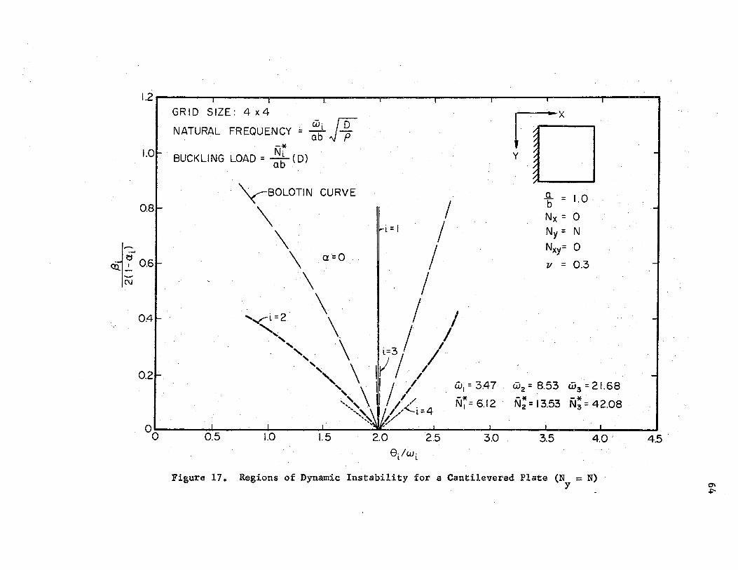
ended plates shown in Figures (17) through (20) illustrate this point.
The axes on Figures (17) and (19) are normalized in numerical order as
has been done on pr~vious figures of this type. Notice, however, that
in both of these examples the second vibration mode is the same as the
first buckling mode, and that the curves denoted by i = 2 become the
characteristic curves, denoted here as Bolotin curve, if the vertical
axis, load axis, is normalized with respect to the first buckling load
and the horizontal axis, frequency axis, is normalized with respect to
the second natural frequency.
It is important to
shape, for instance the
vibration mode, as for
recognize that if there exist a buckling mode
th j mode shape, that is the same as a given
th example the i mode, then there exist a region
th of dynamic instability corresponding to the i natural frequenc7 that
has the characteristic s~ape shown in Figure (11) if the load axis is
th. ·nermalized with respect to th.e j buckling load and tl\e frequency axis
is normalized with respect to the ith natural frequency.
....
L2 ...-----,.-------------,.---...---------,.---...----GRID SIZE: 4 x4
NATURAL FREQUENCY = :~. N . 1.0
. -* BUCKLING LOAD= ~~ (D)
0.8 " -BOLOTI N CURVE y . . I
\ i=I ;·
\
y
b = 1.0
Nx = 0 Ny= N
• c::I
~
-<tl. ~ 0.6
\ a~O /
. \\ ... /
Nxy= 0
v = 0.3
C\J
0.4
0.2··
'v-L=2 ·. \ I / ~' . . I I ', •\ i=3 /-',, \ ,.; I I ', . ' I;· /I
' \ / ,, / ,,,. /..._.4 •,,~ y'-t=
w1 = 3.47 w2 = 8.53 w3 = 21.68 . . . -* . -* -* . . . N1 =6.12 · N2 =13.53 N3 =42.08
',., ? 0 .
0 0.5 1.0 I. 5 2.0 2.5
9-/wi l
3.0 3.5 4.0'.
Figure 17. Regions of Dynamic Instability for a Cantilevered Plate (N = N) y
45
°' ~

,...
,-.
I I
1st 2nd I
/' I
025 050 -
075 1.00
125 1.50
-
" \ \ I \ \ \
VIBRATION MODES - CANTILEVER PLATE
I
-01.., .....
// /
/
/
1st
.,,...---
r-x y
--------
2nd ,, -0.2 "" ,, ~~
,, ----~---or-------
0.1
-OJ__.----- ....... *"· --..... .,,,.,,... -0.2 ----...
BUCKLING MODES - Cl,NTILEVER PLATE
Figure 18. Mede Shapes for a Cantilevered Plate (NY= N)
65

1.2------,.----...----------------~-----------------.
1.0
0.8
-~, r:r ' <l:2. .!.. 0.6 .,
'N
04
0.2
GRID SIZE: 4x4
NATURAL FREQUENCY = ·. Wi . {D . . ab ,Jp
-* BUCKLING LOAD = ~b ( D}
'<BOLOTI N. CURVE .
\ .
. \ \
\ a=O
\. \
,. ' ' ',·
'
\ \ \
.·. ', ,. ', ', ',·
I I l I
. . . I l = 1.3 I
.. ·.· I . .
n=x y
.· b = 3.0
Nx = 0 .
Ny= N Nxy=. 0
11 = 0.3 .
.. 1·· . · 1 .·· . , l .· J,ri=2
. I . / i=4; / .. \ r. _,,
v /, /
w1 = 9.93 . ·Wz = 17.36 w3 = 27. 79 -* . -* -* N1 =II.II N2=27.79 N3= 52.18 ,,
0 . . 0 0.5 1.0 1.5 2.0. 2.5 3.0 3.5 4.0
9/wi
Figure 19. Regions of Dynamic Instability for a Fixed Ended Plate (Ny= N)
. 4.5
i

\.
1st
0.2
0.4 .
0.6
0.6
0.4
0.2
2nd
........ ........ ,
........ ,-) ""0.1 '"0.2 \
\-0.4. '\ \ \ . . \
I ' ' I I .. I I · I I · I I I
I I l I I I
// I .,,,.,,, I
.,.,,, / / .,,,, . .,.., ,,,,..
VIBRATION MODES - FIXED ENDED PLATE
1st 2nd
.,,,.,,,, /
01 / ·.,,, .. '/ .,,. //0.2;/.,,.
I I .· I . / I o.~, I . I I I I I I \ I \ \ \ \ \ \ \ ', \ ' ' ,,. ·., ......
.......... ',
0.01 0.01 -0.05
. ,.., ( I I I I I I I I I I I I I I I I I I I ,_..,
0.10
BUCKLING MODES - FIXED ENDED PLATE
Figure 20. Mede Shapes for a Fixed Ended Plate (N = N) y
67

68
5.3 Plates on Elastic Foundations
The results for a simply supported plate and a clamped plate each
loaded with Nx = N, N = N~ N = 0 and each solved with two different y xy
foundation moduli are illustrated in Figures (21) through (30). Here
the natural frequeracies (w) are for free vibration of the plates rest-
ing upon the foundations. Notice that for these examples, as was the
case with the examples discussed in the previous section, when the mode
shapes for vibration and static buckling become similar, the regions of
dynamic instability approach the characteristic curves. For these
particular examples it is seen th.at when the foundation modulus is in-
creased the region of instability corresponding to the lowest natural
frequency narrows somewhat, whereas the regiens corresponding to higher
frequencies appear to be affected to a lesser degree.

l2 ~
1.0
08
a . ~
-Ol. ~ ~:6 . N
0.4
·0.2
QI...,; 0
GRIO-SIZE: 4 x4
NATURAL FREQUENCY ·= :~ N . -*
BUCKLING LDAD = ~~ ( D)
a=O
0.5 LO 1.5 2.0
9/wi.
25
lrx .
YDS.S .. · ·. S.S. . . . S.S. ·, -
S.S.
· '> Nx = Ny = N Nxy= 0. g. = l.0.
· 71 = 0:3. . Q.Ct2b2 8= ... ,,. .............. , .... , :,.0002
. w1 = 40.10 w2 = 59.47 w3 = 59.4 7 -* . -* . . -*. N1 =71.57 N2 =7L57 N3 =81.50
3.0 3.5 4.0 4.5
Figure 21. Regions of Dynamic Instability for a Simply Supported Plate on an Elastic Foundation (8 = .0002, ~ = O)
$

1.2.----.--.--,.--.--.--.----.--,--,,..----,--,---,--,--,--,-,---,~--.-------.--.----.--.----.--.---
LO
0.8
GRID SIZE : 4 x4
NATURAL FREQUENCY = :~ ff. -*
BUCKLING LOAD = :~ ( D)
I I I
lrX S.S. . YD S.S. . . S.S.
S.S .
Nx = Ny = N Nxy= 0
<ii"I "if o. s1
a=0.6 JI I I ,. I .
t = 1.0 v = 0.3
(\J
0.4
0.2
,--t ·= 2 3 I I ~ ,
I 'I 'I 'I ~
q a2b2 8= MS-~~·-•= .0002
w, = 40.70 w2 = 59.47 w3 = 59.47 -* -* -* N, = 71.57 N2 = 71.57 N3 = 81.50
Q..___,__,_,___,__,__,...___,__, __ __,__,--,--__,--,__,......_~__,_.___,__,__,..i......__,__,.......i.__,__,--J
0 0.5 1.0 1.5 2 .0 2 .5 3 .0 3 .5 4.0 4.5
9Jwi
Figure 22. Regions of Dynamic Instability for a Simply Supported Plate on an Elastic Foundation(~= .0002, ~ = 0.6) -.J
0

71
1st 2nd
-0.05 0 ,,,-"'\
/ ' I \ I \
I \ I \ I I I I I I
\ I \ I \ I , \ I
' / ,_.,
VIBRATION MODES - SIMPLY SUPPORTED PLATE
r-x y
I st 2nd -0.05
....... -.... / '\ I \ I I D I I ! ! I ! I ! I \ I \ I \ I . I \_,,,/
0
0.05
--------- ..... .,,.. ~
/ · . '"0.05 I \
. \ I \ I ,.... / """"'"'----------,,
BUCKLING MODES - SIMPLY SUPPORTED PLATE
Figure 23. MCJde Shapes for a Simply Stl\ppc,,cted Plate wn an Elastic · Foundation (~ === ~ 0002 ~ N = N = N) . . x. y

. I.
0.8
--,tf . · ct2. ~ 0.6
N.
04
0.2
GRID SIZE: 4 _ w;
NATURAL FREQU o.u " . . . -*
BUCKLING LOAD= Ni . - . . . . QL
.... ' ',,,
' ''\,
·a= 0
\ \
\ \ \ \ x· \. \ ·,
\ \ \
. \ \ ' \
. \ \ \
I I I I I
·/ I l
. I I '
. !,--i. =2 3 l . ' r I
I I
Nx = Ny = N Nxy= .o . _Q_ = 1.0 b .. · .. v = 0.3
- ga2b2 -8- -- ---·-·- .0006
.I I
I I
I 1
. I
I I .. ·
I 'l
1 -.:r. .. ~
w1 = 65.09 w2 = 78.21 w3 = 78.21. · .. -* -* . -* . . .· Nr =113.93 N2 =12378 N3 = 123.78
0 . . 0 0.5 1.0 1.5 2.0 2.5 3.0 3.5 4.0
Figure 24.
45
9/wi
Regions of Dynamfo Instability for a Simply Supperted Plate on an Elastic Feundac Uon (S = .0006, ex.= 0)
....... N

1.2-----,.----,----.,..-------------,---...-~,-------,-----
1.0,.
0.8
--,~ <u. ..!_ 0.6 1.-C\J c
0.4
- 02
GRID SIZE: 4 x4
NATURAL FREQUENCY = :~ if -*
BUCKUNG LOAD= : ( D)
i = 1-...J a_=o.6/ I l I .
..,.-L: 2 3 \ I , \ I \ I . I I \ I I I ' I I I I I I I \ I \ . I \ I l I ' I I I \ I \ I
I
x vG=ss D s.s. S.S.
S.S.
Nx = Ny = N Nxy= 0
b = 1.0
v = 0.3 _ .· Q a.2b2 _
8- ,.,c,,.,,...,...,~,'."'.0006.
w1 = 65.09 w2 = 78.21 w3 = 78.21 -* -* -* N1 = 113.93 N2 =123.78 N3 = 123.78
o------------~~~-----------~-------~~~.......i..----~ .......... ~~_,_~-----o 0.5 1.0 1.5 2.0 2.5 3.0 3.5 4.0 4.5
Figure 25.
9/wi
Region~ of Dynamic I-1,1.stability for a Simply Supported Plate on an Elastic Foundation {a = .• 0006, a. = o.6) o,.J
II.,)

I st ·
, ,,,~·0.05 I ..
I .
·{ . \ I ' I \ ! \ .· /
\ / ,_.,
2nd
0
. VIBRATION MODES - SIMPLY SUPPORTED PLATE
I
-,0.05 / ., .
I .. \ I ,_..,~
I
I st
0
2nd .. I
/-,0.05
l \. ... ,_.,/
I
BUCKLING MODES .. SIMPLY SUPPORTED PLATE
Figure 26. Mode Shapes f~r a Simply Supp~rted Plate en an Elastic Foundation(~= .0006, N = N = N)
x 1
74

1.2--~~--~~~--~~---~~~--~~~--~~--~~~...-~~-...~~-----
--
GRID SIZE: 4 x 4
NATURAL FREQUENCY = :~ ff . -*
I.Or BUCKLING LOAD= Ni ( D) ab
0.8
i = I
a=O
--,~ QJ.. ..:. 0,6
-N
.0.4
0.2
I I I
I
I I I .
'fY-L: 2 3 I . ,
I
l ;,:,c,«'c y
N,, = N
Ny= N
g = 1.0
v = 0.3 I 8- qa2b2 -I
I {.I l
'I ~
'I 'I
'I 'I t v
- ,.,.., ............... "" - .0002
w1 = 49.67 w2 = 78.70 w3 = 78. 70 -* - * .· -* N 1 = 95.45 N 2 = 105.55 N 3 = 105. 55 ·
o~--~~~~---..,....~-------~~----~~a...-~~~~--~~~~~~~~ 0 0.5 1.0 1.5 2.0 2.5'. 3.0 3.5 4.0 4.5
9/wi
Figure 27. Regions of Dynamic Instability for a Clamped Phte on an Elastic Foundation cs = .0002) -.J
VI

I st
-0.05 ,"',
2nd
I ',, I \ ' \. ' \ \ , ) \ ,"" ' ...... --
VIBRATION MODES - CLAMPED PLATE·
I st 2nd
_....,:0.05
, ' / \ I \ I \ I I I I
\ : \ I \ I \ / ,_.,
BUCKLING MODES - CLAMPED PLATE
Figure 28. Mode Sb.ape$ f®>r a Clamped Pht@ O!:l. an Elastic [email protected] (8 = .0002. N = N = N) - x y .
76

1.2-----------------------------------GRID SIZE: 4 x 4
NATURAL FREQUENCY = :b n ....:*· .
. I.Or BUCKUNG LOAD = Nbi ( D) a .
0.8
I I
. I • I I I I
y
Nx = Ny = N Nxy= 0 a· b= 1.0
·-1~ en.~-· 0.61- I v = 0.3 .
8=. qa2b2 . -C\I / ... r l = 2,3 4. r. . , '·-. 25;200(0) =,0006
0.4 I I
I I I
0.2 I I
/ ~
w1 = 71.04 w2 = 93,67 w3 = 93.67_ -* . -* .·._* N 1 =145B6 N2 =145.83 N3 =145.83
o· I
0 0.5 1.0 15 2.0 2.5 3.0 3.5 40 . '4.5
ei/wi
Figure· 29,.. Regi~ms of Dynamic Instability for a Clamped Plate en an Elastic Foundation. . (8 = .0006) ..... ......

'-
-
1st 2nd
0 -0.05 /- ..... ,
I ' I \ I . \ I \ I \ \ l "---------*"
VIBRATION MODES - CLAMPED PLATE
rx 1st
y 2nd
I I
(55 _ -0.05 / -,
I ' I ' \ I \ .... ___ .... /
0 0
·0.05 (55 .... --..... I \ I I -\ I ~, .... _,,;./. '
I I
BUCKLING MODES - CLAMPED PLATE
Figure30o Mode Shapes for a Cl.amped.Plate on an Elastic Foundation (a= o0006v N = N = N) . .· x y
78

79
5.4 Plates With Viscous Damping
Regions of dynamic instability corresponding to the fundamental
vibration frequency are found for a simply supported plate and a clamp-
ed plate, each subjected to a loading Nx = N7 = N, and Nxy = O, and
viscous damping. These results are illustrated in Figures (31) and
(32). Tb.e damping coefficients are expressed as a percentage of criti•
cal damping. For relatively small damping ceefficients, the effect ef
damping is that the amplitude of the pulsating lead must have a finite
value before the plates will become dynamically unstable. Fer example,
fer the problem illustrated in Figure (31) when Yi= 0.05 the amplitude
of the pulsating lead must reach O.l times the static buckling load
before any instability will occur. As the damping coefficient is in-
creased the lead required to produce any instability becomes very large.
5.5 Plate 0n Elastic Foundation With Viscous Damping
Figure (33) shews the regien of dym.amic instability f0r a simply
supported plate on an elastic foundation subjected te the effect of
viscous damping and a loading of N = N = N and N = O. The purpose x y xy
of this example is to illustrate the simplicity in handling this class
of relatively complex problems by the metnod developed in this thesis.

1.2---........ ------.._,.---........ ---....------,..---...... --....... -----
1.0!
0.8
--,6 CO...!.. 0:6' -N
0.4.
0.2
·GRID SIZE: 4 x4 w· ro
NATURAL FREQUENCY = a.~ ,Jp r.. -* BUCKUNG LOAD= .. : (0)
, . .;;,,;.PJJ:'
,, ,, I ,, ,, ,,
JI II
·. II ,, It
11 ,,
fr=:s.s. -__
D s.s. 5$ ·. S.S.
Nx = Ny = N
Nity=>O
%= LO · v = 0.3
--- DAMPING COEF. 77=0.05
----:-~ 7J:::: O.J_ · .. ,, /1
1/ · .;...__ 7J = 0.3 · --- NO DAMPING
w, = 19.15 ·
-* N1 = 18.58 -0---....... ---_ ....... __ _,i.,,_......-....... _______________ _.. _____ _
0 0.5 LO 1.5 2.0 2.5 3.0 ·. 3.5 4.0 c-·.'' 4.5
e,lwi
Figure 31. Regions of Dynamic Instability for a Simply Supported Plate With. ViscGus Damping a:> 0

1.2------,-----------.----.-------~---..,....--.....,.----.
GRID SIZE : 4x4 fr·\««~ NATURAL FREQUENCY .. = :~ ff -*
1.01- BUCKLING LOAD= :b ( D)
\' ~' I
0.81-I
·. 'I /I
I Nx = Ny = N
'I I I \ ~'\ I I Nxy= 0
/1 ~ = 1.0
0,1~ ot \, ~ . / I a=O \\ I I v = 0 .3 ~\a=0.6 I I ,, /, ,,
I - DAMPING COEF. 77 =0 .05 ,\ I 1 --77=0. I 0.4 I- \ \ I I 1
\ \ I I ~ } --- NO DAMPING \ I \ ', I I \ ... ./ ' I \ I
021- \ I \ I \"-../j w, = 35.20 \ \ I \ l - * \ I ,. . N1 = 49.84
I 0
0 0 .5 1.0 I. 5 2 .0 2 .5 3.0 3 .5 40 4.5
8 1IW1
Figure 32. Regions of Dynamic Instability f or a Clamped Plate With Viscous Damping
00 .....

L2r-----,----..----.....,..-------,.----,--.--.._----,----
1.0
0.8
GRID SIZE: 4 x 4
NATURAL FREQUENCY = :~ ff--*
BUCKLING LOAD= :b ( D)
', ',, ,, ',
.a= O
·~
q q q q
x
~DB v ss.·•u . . . S.S.
Nx = Ny = N Nxy= 0
cil! 0.6 '\
\
~,. \ \
g = LO
11 = 0.3 2 2 .
8- q a o _ N
0.4
0.2
\ \ \ \ \ \
\
·--DAMPING COEF. ?]=0.1 ---NO DAMPING
\ \ \ \ \ \ \ I \/
- ""' .,.l"\("\/1"\\ - .0002
w, = 40.70 -* N1 =71.57
o~-----~---~~~----.....J..~~~~~-----J'"-'.....---..J...~~--..1.---~.....J-------.J 0 .Q.5 1.0 , I. 5 2.0 2.5 3.0 3.5 4.5 4.0
e,1w,
Figure 33. Regien of Dynamic Instability fer~ Simply Supperted Plate 0n an Elastic F0undation With Viscous Damping 00
N

CHAPTER VI
SUMMARY AND CONCLUSIONS
6.1 Summary and Conclusions
A methGd has been developed in this thesis, using a finite element
stiffness analysis, to determine the principal regions of dynamic in
stability of rectangular, hemogeneeus plates. The procedure employed
in tb.e development consists of the derivation of the governing set of
ordinary differential equations by applying the Lagrangian equation to
the individual finite plate elements, and ef the solution of these
equations for regions ef instability using the methods from the theory
of linear differential equations with periodic coefficients. The
development of a finite element solution for structural problems using
the Lagrangian equation has not~ to this writer's knowledge, appeared
her~tefere in the literature. Alth0ugh the approach taken by others
for the solution of various problems using the finite element method is
very similar mechanically to the Lagrangian approach, the Lagrangian
method offers a unified approach which is more adaptable for extensions
of the finite element procedure. A series of examples which includes
plates subjected to several loading and boundary conditions» and plates
with and without the effects of viscous damping and an elastic founda
tion were solved. A limited parametric investigation was made upon
these examples.
The method is capable of handling a wide range of complex problems
83

84
with regard to boundary conditions and loading. The method makes no
presuppositions with regard to the eigenfunctions for free vibration
and static buckling as is the case with most existing analytical solu
tions. It has been shown that the size of the regions of dynamic
instability depend upon the similarity of the mode shapes of free vibra
tion and static buckling. For the special cases when the mode shapes
for vibration and static buckling are the same the regions of insta
bility are the characteristic curves shown in Figure (11). In these
eases the governing differential equation can be reduced to one second
order Mathieu~Hlll equation. Although no attempt was made to develop
a criterion for likeness or similarity of mode shapes, it was observed
that when the mode shapes were very similar the instability regions
were largest, and when the mode shapes were very dissimilar the insta
bility regions were smallest.
The finite element method for analyzing plates for dynamic
stability makes it possible to solve large numbers of complex problems,
.and to analyze the problems with respect to the various parameters
which affect the stability of the plates. This type of analysis with
other solution methods at the present is unpractical.. The treatment of
the various boundary conditions which poses probaoly the biggest prob
lem to analytical solutions is trivial in a finite element analysis.
It is possible that the results of finite element analyses of plates
might aid in giving direction to analytical research in this area.
6.2 Suggestien for Further Research
The examples that have been solved in this thesis have been
limited to rectangular, homogeneous plates loaded with uniformly dis
tributed loads across the edges. The metnad developed is capable,

85
however, of handling a much wider range of problems. Other geometrical
shapes can be solved, but it might be necessary to use finite element
shapes other than rectangular to acconunodate the various shapes. In
the literature some of the necessary elemental matrices have been
developed for finite elements of other shapes.· Plates of variable
thickness can be analyzed by using the variable mass and rigidity terms
in the integrals used in evaluating the elemental matrices. Other types
of leading conditions should be analyzed. The loadings used in this
thesis were uniformly distributed across the plate edges and the in
plane stress distribution due to these loads was known.to be constant
througho~t the plates. The in-plane stress distribution caused from
other lead cenfigurations could be determined using methods similar to
those given in works by Lundgren (19) and Apanian (20). Once the stress
distributions are knewn the elemental stability matrices could be
evaluated for these conditions and the regions of dynamic stability
determined. A dynamic stability analysis of multilayered sandwich
plates can be perfermed using the metheds of this thesis and those pre
sented by Lu.ndgren (19).
Other basic fact0rs which should be investigated in relatien to
the dynamic stability of plates are the effects of in-plane inertia,
non-linear damping, and the use of materials which exhibit non-linear
or elasto-plastie stress~strain distributions.

A SELECTED BIBLIOGRAPHY
(1) Bolotin, v. V., Dynamic Stability of Elastic Systems. Holden-Day, Inc., San Francisc0, 1964.
(2) Ray1eigh»·Jehn William Strutt: (Lord), 110n the Maintenance of Vibrations by Forces of Double Frequency and on the Propagation of Waves Through a Medium Endewed With a Periodical Structure.," P'bil0sophical Magazine, Vol. S, N0. 24, 1887, PP• 145-149.
(3) Beliaev» N. M., "Stability of Prismatic Rods Subjected to Variable Longitudinal Ferces." Collectien of Papers: Engineering Construction and Structural Mechanics, Leningrad, 1924.
(4) Beilin, E. A. and G. U. Dzhanelidze, "Survey of the Works en the Dynamic Stability of Elastic Systems.u Prikl •. Mat. i Mekhan., Vol. 16, Ne. 5, 1952, pp. 635-648. (Available in English as ASTIA No. AD-264148.)
(5) Bedner, V. A., "'the Stability of Plates Subjected te Longitudinal Periodic Ferces." Prikl ... Mat. i Mekh.an., (N.S.) Vol. 2, 1938» PP• 87-104.
(6) Kb.alilov, z. I., "The Dyaamic Stability of a Plate Under the Action of Periedic Longitudinal Forces.n Tr. Azerb. Gas. Univ •• Ser. Mar., Vel. 1, 1942, pp. 28-32.
· (7) Einaudi, R., "Sulle Confiiurazioni di Equilibrio Instable di una Piastra Sollecit.ata da Sforzi Tangenziali Pulsanti. •·• Atti. Accad. Gieenia, Vol. 1, Memoria XX, 1935-36, pp. 1-5.
(8) Ambartsumian, s. A. and A. A. Kh.aehatrian, "On the Stability and Vibrations of Anisotropic Plates. 11 Izv. Akad. Nauk, SSSR, Otd. Tekhn. Nauk. Mekhan. i Mashinostr., VC>l. 1, 1960 9 pp. 113-122.
(9) Mettler, E., "Biegeschwingungen eines Stabes mit kleiner Vorkrmnmung,exzentrisch angreifender publsierender Axiallast und statischer Querbelastung. 11 ~,hungshefte aus d. Geb. d. Stahlbaues, Vol. 4, 1941, pp. 1-23.
(10) NawnGv, K. A., "The Stability of Prismatic Rods Allowing fer Dam.ping." Tr. Mosk. Inst. In.zh. Transp.~ Vol. 69~ 1946, pp. 132-141.
86

87
(11) Mettler, E.~ and F. Weidenhammer:1 11Der axial Pulsierend belastete Stab mit Endmasse." z. angew. Mat. Mekhan., Vol. 36, 1956, pp. 284-287.
(12) Chelomei, V. N., The Dynamic Stability ef Elements of Aircraft Structures. Aeroflot, Moscow, 1939~
{13) Turner, M. J., R. W. Clough, H. c. Martin, and L. J. Topp, "Stiffness and Deflection Analysis of Complex Structures.'' Jour. Aero. Sciences, Vol. 23, No. 9, 1956, PP• 805-823.
(14) Flugge, w., ed., Handbook of Engineering Mechanics. McGraw-Hill Book Company, Inc.~ New Y@rk, 1962.
(15) Cesari:; Lambet·to, As;nnpototic Behavior and Stability Problems in Ordinary Differential Equations. Springer-Verlag, Berlin. ©lottingen. Heidelburg, 1959.
(16) Chetayev~ N. G., The Stability of Motion. The Pergamon Press~ 1961. (Translated from the Russian.)
(17) McLachlan, N. w., Theory and Application of Mathieu Functions. Dover Publications 0 Inc., New York, 1964.
(18) Brown~ John E. ~ 11Dynamic St.ability of Bars by the Finite Element Meth.oc!.. '' ~aster 0 s Repor~~ Oklahoma State University 9
Stillwater~ Oklahoma» 1968.
(19) Lundirenv Harry R. ~ ''Bu.ckling @f Multilayer Plates by Finite Elements. 11 Ph.D .. Thesis 9 Oklahoma State Urdversity~ Stillwater j Oklahoma~ 1967.
{20) Apanian, Ronald A.ii ''Fr.ame Andys.is ef 'thin Shells. 11 Ph.D. Thesis!> Oklahoma State Univet·sity» Stillwater~ Oklahoma, 1967.

VITA
Johnny Mack Hutt
Candidate for the Degree of
Doctor of Philosophy
Thesis: DYNAMIC STABILITY OF PLATES BY FINITE ELEMENTS
Major Field: Engineering
Biographical:
Personal Data: Born at Tuscaloosa, Alabama, September 12, 1940, the son of Joe and Mildred Hutt.
Educatiom Attended grade school at Tuscaloosa& Alabama; graduat~ ed from Tuscaloosa High School in 1958; received the Bachelor of S~ience degree from the University of Alabama, at University~ Alabama~ with a major in Civil Engineering, in August~ 1963; received the Master of Science degree from the University of Alabama, at University, Alabama, with a major in Civil Engineering 9 in May, 1965; completed the requirements fer the Doct©r of Philosophy degree in May~ 1968.
Professional Experience: Graduate research assistant and parttime instructor in th.e school of Civil Engineering, Univer~ sity etf Alabama 9 1964=1%5. Graduate teaching assistant and part=time i11.st.ruct:,;ir in the scheol of Civil Engineering, Oklah~nua State University~ 1965-1967. Associate Member of Americ~n Society of Civil Engineers.