Dynamic Response of Second Order Mechanical Systems …rotorlab.tamu.edu/me617/handout2a_2008.pdf · where ( I, Dθ,Kθ) are equivalent mass moment of inertia, rotational viscous

MEEN 617 Notes: Handout 2a © Luis San Andrés (2008)

2-1

Handout #2a (pp. 1-39)

Dynamic Response of Second Order Mechanical Systems with Viscous Dissipation forces

2

( )2 ext td X d XM D K X Fd t d t

+ + =

Free Response to initial conditions and F(t) = 0, Underdamped, Critically Damped and Overdamped Systems

Free Response for system with Coulomb (Dry) friction Forced Response for Step Loading F(t) = Fo


2-2

Second Order Mechanical Translational System: Fundamental equation of motion (about equilibrium position, X=0)

( )X ext t D KdVF M F F Fd t

= = − −∑

Dd XF DV Dd t

= = : Viscous Damping Force

kF K X= : Elastic restoring Force

2

2Id XF M a Md t

= = : Inertia Force

where ( M, D ,K ) represent the equivalent mass, viscous damping coefficient, and stiffness coefficient, respectively.

Since d XVdt

= write the equation of motion as: 2

( )2 ext td X d XM D K X Fd t d t

+ + =

+ Initial Conditions in velocity and displacement; at t=0:

(0) and (0)o oV V X X= =


2-3

Second Order Mechanical Torsional System: Fundamental equation of motion (about equilibrium position, θ=0)

( )ext t D KdTorques I T T Td t θ θω

= = − −∑

Tθ D = Dθ ω : Viscous dissipation torque T θ K = Kθ θ : Elastic restoring torque T θI = I dω /dt : Inertia torque where ( I, Dθ ,Kθ ) are equivalent mass moment of inertia, rotational viscous damping coefficient, and rotational (torsional) stiffness coefficient, respectively.

Since ω = dθ /dt , then write equation of motion as:

2

( )2 ext td dI D K Td t d tθ θθ θ θ+ + =

+ Initial Conditions in angular velocity and displacement at t=0: (0) and (0)o oω ω θ θ= =


2-4

(a) Free Response of Second Order Mechanical System Pure Viscous Damping Forces

Let the external force be null (Fext=0) and consider the system to have an initial displacement Xo and initial velocity Vo. The equation of motion for a 2nd order system with viscous dissipation is:

2

2 0d X d XM D K Xd t d t

+ + = (1)

with initial conditions (0) and (0)o oV V X X= = Divide Eq. (1) by M and define:

nK

Mω = : undamped natural frequency of system

cr

DD

ζ = : viscous damping ratio,

where 2crD K M= is known as the critical damping value With these definitions, Eqn. (1) becomes:

22

2 2 0n nd X d X Xd t d t

ζ ω ω+ + = (2)

The solution of the Homogeneous Second Order Ordinary Differential Equation with Constant Coefficients is of the form:

( ) s tX t Ae= (3) Where A is a constant yet to be found from the initial conditions. Substitute Eq. (3) into Eq. (2) and obtain:


2-5

( )2 22 0n ns s Aζ ω ω+ + = (4) Note that A must be different from zero for a non trivial solution. Thus, Eq. (4) leads to the CHARACTERISTIC EQUATION of the system given as:

( )2 22 0n ns sζ ω ω+ + = (5) The roots of this 2nd order polynomial are:

( )1/ 221,2 1n ns ζ ω ω ζ=− −∓ (6)

The nature of the roots (eigenvalues) clearly depends on the value of the damping ratio ζ . Since there are two roots, the solution to the differential equation of motion is now rewritten as:

1 21 2( ) s t s tX t A e A e= + (7)

where A1, A2 are constants determined from the initial conditions in displacement and velocity. From Eq. (6), differentiate three cases: Underdamped System: 0 < ζ < 1, → D < Dcr Critically Damped System: ζ = 1, → D = Dcr Overdamped System: ζ > 1, → D > Dcr Note that ( )1 nτ ζω= has units of time; and for practical purposes, it is regarded as an equivalent time constant for the second order system.


2-6

Free Response of Undamped 2nd Order System For an undamped system, ζ = 0, i.e. a conservative system without viscous dissipation, the roots of the characteristic equation are imaginary:

1 2;n ns i s iω ω=− = (8)

where 1i= − is the imaginary unit. Using the complex identity eiat = cos(at) + i sin(at), renders the undamped response of the conservative system as:

( ) ( )1 2( ) cos sinn nX t C t C tω ω= + (9.a)

where nK

Mω = is the natural frequency of the system. At time t = 0, the initial conditions are (0) and (0)o oV V X X= =

hence 01 0 2and

n

VC X Cω

= = (9.b)

and equation (9.a) can be written as: ( )( ) cosM nX t X tω ϕ= − (9.c)

Where 2

2 00 2M

n

VX Xω

= + and ( ) 0

0

tann

VX

ϕω

=

XM is the maximum amplitude response. Notes: In a purely conservative system, the motion never dies out, it is harmonic and periodic. Motion always oscillates about the equilibrium position X = 0


2-7

Free Response of Underdamped 2nd Order System For an underdamped system, 0 < ζ < 1, the roots are complex conjugate (real and imaginary parts), i.e.

( )1/ 221,2 1n ns iζ ω ω ζ=− −∓ (10)

where 1i= − is the imaginary unit. Using the complex identity eiat = cos(at) + i sin(at), write the solution for underdamped response of the system as:

( ) ( )( )1 2( ) cos sinn td dX t e C t C tζ ω ω ω−= + (11)

where ( )1/ 221d nω ω ζ= − is the system damped natural frequency. At time t = 0, the initial conditions are (0) and (0)o oV V X X= =

Then 0 01 0 2and n

d

V XC X C ζ ωω

+= = (11.b)

Equation (11) representing the system response can also be written as:

( )( ) cosn tM dX t e X tζ ω ω ϕ−= − (11.c)

where 2 21 2MX C C= + and ( ) 2

1

tan CC

ϕ =

Note that as t→ ∞, X(t) → 0, i.e. the equilibrium position only if ζ > 0; and XM is the largest amplitude of response only if ζ =0 (no damping).


2-8

Free Response of Underdamped 2nd Order System: initial displacement only damping ratio varies Xo = 1, Vo = 0, ωn = 1.0 rad/s ζ = 0, 0.1, 0.25 Motion decays exponentially for ζ > 0 Faster system response as ζ increases, i.e. faster decay towards equilibrium position X=0

Free response Xo=1, Vo=0, wn=1 rad/s

-1.5

-1

-0.5

0

0.5

1

1.5

0 10 20 30 40

time (sec)

X(t)

damping ratio=0.0damping ratio=0.1damping ratio=0.25


2-9

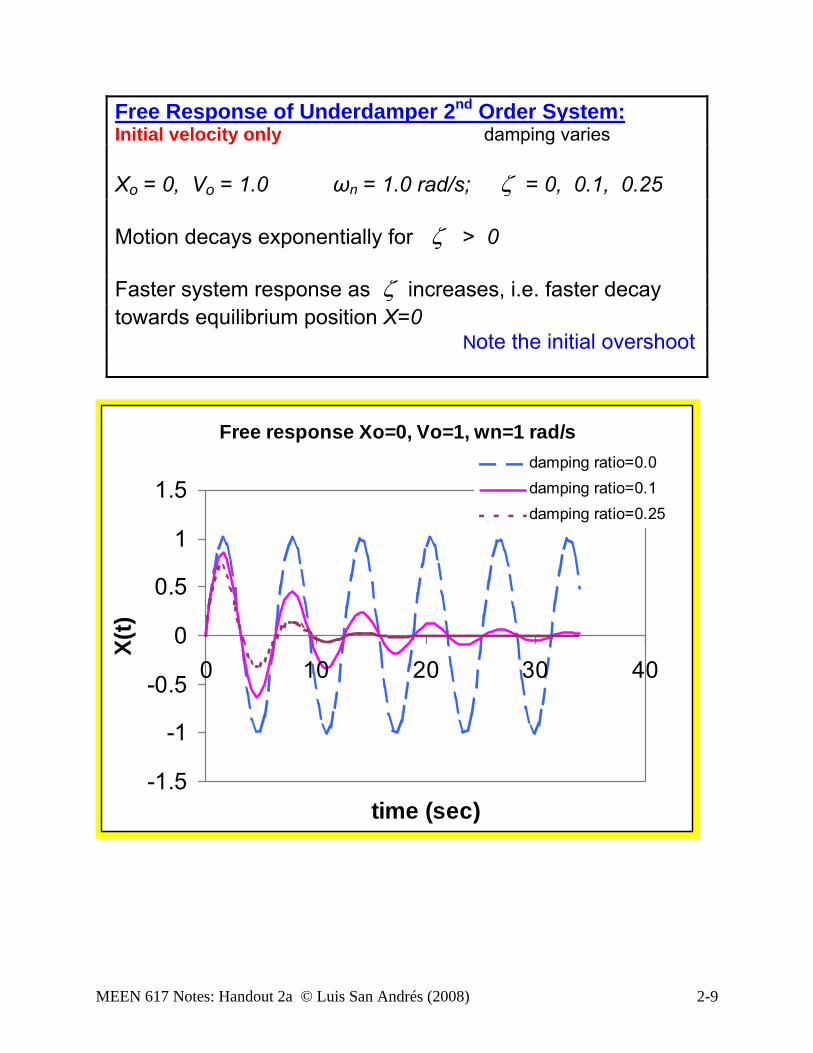
Free Response of Underdamper 2nd Order System: Initial velocity only damping varies Xo = 0, Vo = 1.0 ωn = 1.0 rad/s; ζ = 0, 0.1, 0.25 Motion decays exponentially for ζ > 0 Faster system response as ζ increases, i.e. faster decay towards equilibrium position X=0

Note the initial overshoot


-1.5

-1

-0.5

0

0.5

1

1.5

0 10 20 30 40

time (sec)

X(t)



2-10

Free Response of Overdamped 2nd Order System For an overdamped system, ζ > 1, the roots of the characteristic equation are real and negative, i.e.

( ) ( )1/ 2 1/ 22 21 21 ; 1n ns sω ζ ζ ω ζ ζ⎡ ⎤ ⎡ ⎤= − + − = − − −

⎣ ⎦ ⎣ ⎦ (12)

The overdamped free response of the system as:

( ) ( )( )1 * 2 *( ) cosh sinhn tX t e C t C tζ ω ω ω−= + (13)

where ( )1/ 22* 1nω ω ζ= − has units of 1/time. Do not confuse this

term with a frequency since motion is NOT oscillatory. At time t = 0, the initial conditions are (0) and (0)o oV V X X= =

Then 0 01 0 2

*

and nV XC X C ζ ωω

+= = (14)

Note that as t→ ∞, X(t) → 0, i.e. the equilibrium position. An overdamped system does to oscillate. The larger the damping ratio ζ >1, the longer time it takes for the system to return to its equilibrium position.


2-11

Free Response of Critically Damped 2nd Order System For a critically damped system, ζ = 1, the roots are real negative and identical, i.e.

1 2 ns s ζ ω= =− (15) The solution form X(t) = A est is no longer valid. For repeated roots, the theory of ODE’s dictates that the family of solutions satisfying the differential equation is

( )1 2( ) n tX t e C t Cω−= + (16)

At time t = 0, the initial conditions are (0) and (0)o oV V X X= = Then 1 0 2 0 0and nC X C V Xω= = + (17) Note that as t→ ∞, X(t) → 0, i.e. the equilibrium position. A critically damped system does to oscillate, and it is the fastest to damp the response due to initial conditions.


2-12

Free Response of 2nd order system: Comparison between underdamped, critically damped and overdamped systems initial displacement only Xo = 1, Vo = 0 ωn = 1.0 rad/s ζ = 0.1, 1.0, 2.0 Motion decays exponentially for ζ > 0 Fastest response for ζ = 1; i.e. fastest decay towards equilibrium position X = 0


-1

-0.8

-0.6

-0.4

-0.2

0

0.2

0.4

0.6

0.8

1

1.2

0 5 10 15 20 25 30 35 40

time (sec)

X(t)

damping ratio=0.1damping ratio=1damping ratio=2


2-13

Free Response of 2nd order System: Comparison between underdamped, critically damped and overdamped systems Initial velocity only Xo = 0, Vo = 1.0, ωn = 1.0 rad/s ζ = 0.1, 1.0, 2.0 Motion decays exponentially for ζ > 0 Fastest response for ζ = 1.0, i.e. fastest decay towards equilibrium position X=0. note initial overshoot


-0.8

-0.6

-0.4

-0.2

0

0.2

0.4

0.6

0.8

1

0 5 10 15 20 25 30 35 40

time (sec)

X(t)



2-14

Free Response of 2nd order System: Comparison between underdamped, critically damped and overdamped systems initial displacement and velocity Xo = 1, Vo = 1 ωn = 1.0 rad/s ζ = 0.1, 1.0, 2.0 Motion decays exponentially for ζ > 0 Fastest decay to equilibrium position X = 0 for ζ = 1.0


-1.5

-1

-0.5

0

0.5

1

1.5

0 5 10 15 20 25 30 35 40

time (sec)

X(t)



2-15

E X A M P L E: A 45 gram steel ball (m) is dropped from rest through a vertical height of h=2 m. The ball impacts on a solid steel cylinder with mass M = 0.45 kg. The impact is perfectly elastic. The cylinder is supported by a soft spring with a stiffness K = 1600 N/m. The mass-spring system, initially at rest, deflects a maximum equal to δ = 12 mm, from its static equilibrium position, as a result of the impact. (a) Determine the time response motion of the mass- spring system. (b) Sketch the time response of the mass-spring system. (c) Calculate the height to which the ball will rebound. (a) Conservation of linear momentum before impact = just after impact:

_ omV mV M x+= + (1) where _ 2V gh= = 6.26 m/s is the steel ball velocity before impact

V+ = velocity of ball after impact; and ox : initial mass-spring velocity.

Mass-spring system EOM: + 0M x K x = (2) with 59.62 rad/snKM

ω = =

(from static equilibrium), the initial conditions are (0) 0 and (0) ox x x= = (3)

(2) & (3) lead to the undamped free response: ( ) sin ( ) sin ( )on n

n

xx t t tω δ ωω

= =

given δ = 0.012 m as the largest deflection of the spring-mass system.

Hence, o nx δ ω= = 0.715 m/s (c) Ball velocity after impact: from Eq. (1)) (b) Graph of motion

( )M m m 6.26 7.15 0.892 m s soV V x+ −= − = − = −

(upwards) and the height of rebound is

2

2Vh

g+

+ =

⎡ ⎤⎢ ⎥⎣ ⎦

= 41 mm


2-16

The concept of logarithmic decrement for estimation of the viscous damping ratio from a free-response vibration test

The free vibration response of an underdamped 2nd order viscous system (M,K,D) due to an initial displacement Xo is a decay oscillating wave with damped natural frequency (ωd). The period of motion is Td = 2π/ ωd (sec). The free vibration response is

( )d( ) cos n tox t X e tζω ω−= (1)

where / , 2 cr crD D D K Mζ = = ; ( ) ( ) 2/1 2nd

2/1 n 1 ;M/K ξωωω −==

Consider two peak amplitudes, say X1 and X1+n, separated by n periods of decaying motion. These peaks occur at times, t1 and

Free response of underdamped viscous system

-1

-0.5

0

0.5

1

1.5

0 10 20 30 40

time (sec)

X(t)

damping ratio=0.1

Td

X1

X1+n

t1 t1+n

X2

t


2-17

(t1+nTd), respectively. The system response at these two times is from Eq. (1):

( )11 1 d 1( ) cos n t

oX x t X e tζ ω ω−= = , and

( ) ( ) ( )1-1 1 1 cos ,n d

d

t nTn nT o d d dX x t X e t n Tζω ω ω+

+ += = +

Or, since .2Tdd πω =

( ) ( ) ( ) ( )1 11 d 1 1 cos 2 cos n d n dt nT t nT

n o o dX X e t n X e tζ ω ζ ωω π ω− + − ++ = + = ,

(2) Now the ratio between these two peak amplitudes is:

( ){ }( ) ( ){ } ( )

( )1 1

11

- -11

--1 1

cos

cos 2

n nn d

n dn d

t to d nT

t nTt nTn o d

X e tX e eX eX e t

ζω ζωζω

ζωζω

ω

ω π +++

= = =+

(3) Take the natural logarithm of the ratio above:

( )( ) ( )1 1 1/ 2 1/ 22 2

2 2ln / 1 1

n n d n

n

nX X n T n nπ π ζξω ζ ω δω ζ ζ

+ = = = = ⋅− −

(4)

and, define the logarithmic decrement as:

( )1

1/ 221

1 2 ln 1-n

Xn X

π ζδζ+

⎡ ⎤= =⎢ ⎥

⎣ ⎦ (5)


2-18

Thus, the ratio between peak response amplitudes determines a useful relationship to identify the damping ratio of an underdamped second order system, i.e. once the log dec (δ) is determined then,

( )1/22 2 2

δζπ δ

=⎡ ⎤+⎣ ⎦

(6),

and for small damping ratios, ~2δζπ

.

The logarithmic decrement method to identify viscous damping ratios should only be used if: a) the time decay response shows an oscillatory behavior (i.e. vibration)

with a clear exponential envelope, i.e. damping of viscous type, b) the system is linear, 2nd order and underdamped, c) the dynamic response is very clean, i.e. without any spurious signals

such as noise or with multiple frequency components, d) the dynamic response X(t) →0 as t→∞. Sometimes measurements are

taken with some DC offset. This must be removed from your signal before processing the data.

e) Use more than just two peak amplitudes separated n periods. In practice, it is more accurate to plot the magnitude of several peaks in a semi-log paper and obtain the log-decrement (δ) as the best linear fit to the following relationship [see below Eq. (7)]. From equation (2),

( ) ( ) ( )

( ) ( )

1

1

1 1 1

1 1

cos ,

where cos

n d n d

n

t nT nTn o d

to d

X X t e X e

X X t e

ζ ω ξω

ζ ω

ω

ω

− + −+

−

= =

=


2-19

( )1 1

1 1

ln( ) ln ln( )

ln , where ln ;

n dnTn

n d

X X e

X T A n A X

ζ ω

ζ ω δ

−+ = + =

− = − =

1ln( )nX A nδ+ = − (7) i.e., plot the natural log of the peak magnitudes versus the period numbers (n=1,2,…) and obtain the logarithmic decrement from a straight line curve fit. In this way you will have used more than just two peaks for your identification of damping. Always provide the correlation number (goodness of fit = r2) for the linear regression curve (y=ax+b), where y=ln(X) and x=n as variables


2-20

E X A M P L E A wind turbine is modeled as a concentrated mass (the turbine) atop a weightless elastic tower of height L. To determine the dynamic properties of the system, a large crane is brought alongside the tower and a lateral force F=200 lb is exerted along the turbine axis as shown. This causes a horizontal displacement of 1.0 in. The cable attaching the turbine to the crane is instantaneously severed, and the resulting free vibration of the turbine is recorded. At the end of two complete cycles (periods) of motion, the time is 1.25 sec and the motion amplitude is 0.64 in. From the data above determine: (a) equivalent stiffness K (lb/in) (b) damping ratio ζ

(c) undamped natural frequency ωn (rad/s) (d) equivalent mass of system (lb-s2/in)

a) static force 200 200 lb/in

static deflection 1.0 inlbK = = =

b) cycle amplitude time Use log dec to find the viscous damping ratio 0 1.0 in 0.0 sec 2 0.64 in 1.25 sec

2

1 1 1.0 ln ln 0.22312 0.64

oxn x

δ ⎛ ⎞ ⎛ ⎞= = =⎜ ⎟⎜ ⎟ ⎝ ⎠⎝ ⎠

2 2 2

2 ; ~ 0.03521 4

πζ δ δδ ζπδ π

= = =− +

underdamped system with 3.5% of critical damping.


2-21

c) Damped period of motion, Td = sec/cyc .cyc

s. 62502251

=

Damped natural frequency, 2 10.053

secdd

radTπω = =

Natural frequency, 21

dn

ωωζ

= =−

rad10.059sec

d) Equivalent mass of system:

from n K Mω =

2

2 2 1sec

200 /in10.059n

K lbMω

= = = 1.976 lb/ sec2/in

E X A M P L E A loaded railroad car weighing 35,000 lb is rolling at a constant speed of 15 mph when it couples with a spring and dashpot bumper system. If the recorded displacement-time curve of the loaded railroad car after coupling is as shown, determine (a) the logarithmic decrement δ (b) the damping ratio ζ (c) the natural frequency ω n (rad/sec) (d) the spring constant K of the bumper system (lb/in) (e) the damping ratio ζ of the system when the railroad car is empty. The unloaded railroad car weighs 8,000 lbs.

(a) logarithmic decrement 1

4.8 1.16311.5

oxn nx

δ⎛ ⎞ ⎛ ⎞= = =⎜ ⎟ ⎜ ⎟

⎝ ⎠⎝ ⎠


2-22

(b) damping ratio

( )2 1/ 22 2

2 1 2

πζ δδ ζζ π δ

= ⇒ =− ⎡ ⎤+⎣ ⎦

ζ ≡ 0.1820

(c) Damped natural period: Td = 0.38 sec. and frequency

22 16.53 1secd n

d

radTπω ω ζ= = = −

The natural frequency is

216.816

sec1d

nradωω

ζ= =

−

(d) Bumper stiffness,

2 2car 2 2

1 35,000 lb M 16.816 25612.5sec 386.4 in/secn

lbK Kin

ω ⎡ ⎤= = = =⎢ ⎥⎣ ⎦

(e) Damping ratio when car is full:

full

0.1822 M

DK

ζ = =

Note that the physical damping coefficient (D) does not change whether car is

loaded or not, but ζ does change.

Damping ratio when car is empty 2 e

empty

DK M

ζ =

The ratio

1/ 2

e35,000 0.182 8,000

empty full

e full empty

M MM M

ζ ζ ζζ

⎡ ⎤= ⇒ = = ⎢ ⎥⎣ ⎦

ζ e ≡ 0.381


2-23

EXAMPLE: An elevator weighing 8000 lb is attached to a steel cable that is wrapped around a drum rotating with a constant angular velocity of 3 rad/s. The radius of the drum is 1 ft. The cable has a net cross-sectional area of 1 in2 and an effective modulus of elasticity E = 12 (10)6 psi. A malfunction in the motor drive system of the drum causes the drum to stop suddenly when the elevator is moving down and the length of the cable is 50 ft. Neglect damping and determine the maximum stress in the cable. (Coordinate X(t) describes motion after cable stops, recall that the elastic cable is already stretched due to the elevator weight before the cable stops).

The cable stiffness is just K = 20,000AE lbL in

= and M = inseclb 20.70

in/sec 386 lb 8000 2

2⋅

= , and

2rad31.08 secnω =

At the time of stop, the eqn. of motion is 0M X K X+ = (1)

+ I.C. X(o)=0, and (0) 3 ft/sec 36 in/secX rω= = =

The motion [soln. of (1)] is: nn

( ) sin ( t).oXX t ωω

= (2)

With

maximum Dynamic Displacement is:

od

n

XXω

= (3)

One can also obtain (3) from

conservation of mechanical energy Tmax = Vmax

2 21 1

2 2o

o d dn

XM X K X Xω

= ⇒ =

Xd ≡ 1.15 in = 0.095 ft However, there is also a static deflection due to the elevator weight

8000 lb 0.4 in20000 lb/inS

W M g XK L

= = ≡ =

Then the max. amplitude of deflection is A = XS + Xd = 0.4 + 1.15 in = 1.558 in = 0.1298 ft.


2-24

Maximum Stress in cable:

62

1.558 in 12 10 31,165 psiin 50 12 in

A lb E EL

σ ε= = = × ⋅ =×


2-25

Free Response of a Mass-Spring System with Coulomb Damping (Dry Friction) Recall that a dry friction force opposes motion, and F =μN, N = W = Mg

Consider a mass-spring system resting on top of a surface. The kinetic coefficient of dry friction for relative motion between two surfaces is μ. Assume that at t=0 sec, you release mass M from X(0)=Xo. For a not too large friction coefficient, the mass-spring oscillates about the equilibrium position X=0 with its natural period Tn = 2π/ωn.

The figure below depicts the motion. The system dynamics is governed by different EOMs if motion is to the left (X decreasing) or to the right (X increasing) since the friction force changes sign. It is of importance to know the amplitude decay (δ) every period of motion and also the time elapsed until the system stops.

Free response of a mass-spring system with dry-friction


2-26

Let’s analyze the motion for a full period. On the first ½ period, the mass-spring moves to the left and the friction force points towards the right. On the second ½ period, the mass-spring moves to the right and the friction force points towards the left. The amplitude of response shows a finite amplitude decay each ½ period of motion.

MOTION TO THE LEFT: 0 ≤ t ≤ ½ τ = ½ Tn first ½ period

for 0M X K X F W

Xμ+ = =

<(1)

with I.C., ( ) ( ) 0 , 0 0oX X X= =

MOTION TO THE RIGHT: ½ τ ≤ t ≤ τ=Tn, second ½ period

- for 0M X K X F W

Xμ+ = − =

>(2)

with I.C.,

( ), 02 2oX X X Xτ τ⎛ ⎞ ⎛ ⎞= − −Δ =⎜ ⎟ ⎜ ⎟

⎝ ⎠ ⎝ ⎠

The solution of Eq. (1) or (2) is

( ) ( )( ) cos sinn nX t A t B t F Kω ω= + +

MOTION TO THE LEFT: applying the initial conditions obtain

( )( ) ( ) cos (2)o nF FX t X tK K

ω= − +

after ½ period, at

2 n

t τ πω

= =, the position of the mass-spring

(XL) is:


2-27

( )( ) ( ) cos

2 = (3)

L o

L o o

F FX X XK K

FX X X XK

τ π= = + − +

= − + = − + Δ

Let 2FXK

Δ = be the amplitude decay for the first ½ period and note that

the velocity ( )=0x τ The sketch below shows the response X(t) for the first ½ period of motion

MOTION TO THE RIGHT: 0X > , second ½ period

2tτ τ< ≤

- for 0M X K X N

Xμ+ =

>(4)

with I.C.,

( ), 02 2oX X X Xτ τ⎛ ⎞ ⎛ ⎞= − −Δ =⎜ ⎟ ⎜ ⎟

⎝ ⎠ ⎝ ⎠

)


2-28

or

( ' 0); 0 ( ' 0)2 2LX X X t X X tτ τ⎛ ⎞ ⎛ ⎞= = = = = =⎜ ⎟ ⎜ ⎟

⎝ ⎠ ⎝ ⎠

where for simplicity, define a shift in the time scale as t’ = t – t* with

* 2n

t π τω

= = (5)

Then solution of Eq. (4) defining the system dynamics for motion to the right is:

( ) ( )( ) cos sinn nX t A t B t F Kω ω′ ′ ′ ′ ′= + − (6)

and applying the initial conditions at t′ = 0 , obtain:

( )( ') ( )cos ' - L nF FX t X tK K

ω= + (7)

Now, at t =Tn (1 full period), i.e. t′ = ½ τ ; i.e. the mass-spring system is at its rightmost position (XR), as shown in the graph below

( )

o

( )cos2

2

X 2

R L

R L L

R

F FX X XK K

FX X X XK

X X

τ π⎛ ⎞ = = + −⎜ ⎟⎝ ⎠

= − − = − −Δ

= − Δ

(8)

and note that ( ) 0X τ =

X0

-X0

t

XR

0

XL

t’

/2

/2

X

2 X =


2-29

Then, after 1 full period of motion the amplitude decays from Xo to XR = Xo -2 ΔX = Xo - δ

where 42 4F WXK K

μδ = Δ = =

The motion proceeds to a stop until Friction force (μN) > Spring restoring force (K Xstop) Does the system return to the equilibrium position X=0 given by the unstretched spring, or is it possible that there maybe more than one equilibrium position?


2-30

(b) Forced Response of 2nd Order Mechanical System b.1. Step Force Let the external force be a suddenly applied step force of magnitude Fo, and consider the system to have initial displacement X0 and velocity V0. Then for a system with viscous dissipation mechanism, the equation of motion is

2

2 od X d XM D K X Fd t d t

+ + = (21)

with initial conditions (0) and (0)o oV V X X= = Divide Eq. (1) by M and define:

nK

Mω = : undamped natural frequency of system

cr

DD

ζ = : viscous damping ratio,

where 2crD K M= is known as the critical damping value With these definitions, Eqn. (1) becomes:

22 2

2 2 o on n n

F Fd X d X Xd t d t M K

ζ ω ω ω+ + = = (22)

The solution of the Non-homogeneous Second Order Ordinary Differential Equation with Constant Coefficients is of the form (homogenous + particular):

( ) s t oH P

FX t X X Ae K= + = + (23)

Where A is a constant found from the initial conditions and XP=Fo/K is the particular solution for the step load.

Note: Xss=Fo / K is equivalent to the static displacement if the force is applied very slowly.


2-31

Substitution of (23) into (22) leads to the CHARACTERISTIC EQUATION of the system:

( )2 22 0n ns sζ ω ω+ + = (25) The roots of this 2nd order polynomial are:

( )1/ 221,2 1n ns ζ ω ω ζ=− −∓ (26)

The nature of the roots (eigenvalues) clearly depends on the value of the damping ratio ζ . Since there are two roots, the solution to the differential equation of motion is now rewritten as:

1 21 2( ) s t s t

oX t A e A e F K= + + (27) where A1, A2 are constants determined from the initial conditions in displacement and velocity. From Eq. (27), differentiate three cases: Underdamped System: 0 < ζ < 1, → D < Dcr Critically Damped System: ζ = 1, → D = Dcr Overdamped System: ζ > 1, → D > Dcr


2-32

Step Forced Response of Underdamped 2nd Order System For an underdamped system, 0 < ζ < 1, the roots are complex conjugate ( real and imaginary parts), i.e.

( )1/ 221,2 1n ns iζ ω ω ζ=− −∓ (28)

where 1i= − is the imaginary unit. The solution for underdamped response of the system adds the homogenous and particular solutions to give:

( ) ( )( )1 2( ) cos sinn td d ssX t e C t C t Xζ ω ω ω−= + + (29)

where ( )1/ 221d nω ω ζ= − is the system damped natural frequency. and ss oX F K= At time t = 0, the initial conditions are (0) and (0)o oV V X X= =

Then ( ) 0 11 0 2and n

ssd

V CC X X C ζ ωω

+= − = (30)

Note that as t→ ∞, X(t) → Xss = Fo/K for ζ > 0, i.e. the system response reaches the steady state (static) equilibrium position. The larger the viscous damping ratio ζ , the fastest the motions will damp out to reach the static position Xss.


2-33

Step Forced Response of Undamped 2nd Order System: For an undamped system, i.e. a conservative system, ζ = 0, and the

dynamic forced response is given from equation (29) as:

( ) ( )( )1 2( ) cos sinn n ssX t C t C t Xω ω= + + (31) with Xss = Fo/K, C1 = (X0 – Xss) and C2 = V0 /ωn (32) if the initial displacement and velocity are null, i.e. X0 = V0 = 0, then

( )( )( ) 1 cosss nX t X tω= − (33) Note that as t→ ∞, X(t) does not approach Xss for ζ = 0.

The system oscillates forever about the static equilibrium position Xss and,

the maximum displacement is 2Xss, i.e. twice the static displacement

(F0/K).


2-34

Forced Step Response of Underdamped Second Order System: damping ratio varies Xo = 0, Vo = 0, ωn = 1.0 rad/s ζ = 0, 0.1, 0.25 zero initial conditions

Fo/K = Xss =1;

faster response as ζ increases; i.e. as t → ∞, X → Xss for ζ > 0

Step response Xss=1, Xo=0, Vo=0, wn=1 rad/s

0

0.5

1

1.5

2

2.5

0 10 20 30 40time (sec)

X(t)



2-35

Forced Step Response of Overdamped 2nd Order System For an overdamped system, ζ > 1, the roots of the characteristic eqn. are real and negative, i.e.

( ) ( )1/ 2 1/ 22 21 21 ; 1n ns sω ζ ζ ω ζ ζ⎡ ⎤ ⎡ ⎤= − + − = − − −

⎣ ⎦ ⎣ ⎦ (34)

The overdamped forced response of the system as:

( ) ( )( )1 * 2 *( ) cosh sinhn tssX t e C t C t Xζ ω ω ω−= + + (35)

where ( )1/ 22* 1nω ω ζ= − . Do not confuse this term with a frequency

since motion is NOT oscillatory. At time t = 0, the initial conditions are (0) and (0)o oV V X X= =

Then ( ) 0 11 0 2

*

and nss

V CC X X C ζ ωω

+= − = (36)

Note that as t→ ∞, X(t) → Xss = Fo/K for ζ > 1, i.e. the steady-state (static) equilibrium position. An overdamped system does not oscillate or vibrate. The larger the damping ratio ζ , the longer time it takes the system to reach its final equilibrium position Xss.


2-36

Forced Step Response of Critically Damped System For a critically damped system, ζ = 1, the roots are real negative and identical, i.e.

1 2 ns s ζ ω= =− (37) The step-forced response for critically damped system is

( )1 2( ) n tssX t e C t C Xω−= + + (38)

At time t = 0, the initial conditions are (0) and (0)o oV V X X= = Then ( )1 0 2 0 1andss nC X X C V Cω= − = + (39) Note that as t→ ∞, X(t) → Xss = Fo/K for ζ > 1, i.e. the steady-state (static) equilibrium position. A critically damped system does not oscillate and it is the fastest to reach the steady-state value Xss.


2-37

Forced Step Response of Second Order System: Comparison of Underdamped, Critically Damped and Overdamped system responses Xo = 0, Vo = 0, ωn = 1.0 rad/s ζ = 0.1,1.0,2.0 zero initial conditions

Fo/K = Xss =1; (magnitude of s-s response)

Fastest response for ζ = 1. As t → ∞, X → Xss for ζ > 0

Step response Xss=1, Xo=0, Vo=0, wn=1 rad/s

0

0.2

0.4

0.6

0.8

1

1.2

1.4

1.6

1.8

2

0 5 10 15 20 25 30 35 40time (sec)

X(t)



2-38

EXAMPLE: The equation describing the motion and initial conditions for the system shown are:

2( / ) , (0) (0) 0M I R X D X K X F X X+ + + = = = Given M=2.0 kg, I=0.01 kg-m2, D=7.2 N.s/m, K=27.0 N/m, R=0.1 m; and F =5.4 N (a step force), a) Derive the differential equation of motion for the system (as given above). b) Find the system natural frequency and damping ratio c) Sketch the dynamic response of the system X(t) d) Find the steady-state value of the response Xs-

s. (a) Using free body diagrams: Note that θ= X/R is a kinematic constraint. The EOM's are:

GM X F K X D X F= − − − (1)

GI F Rθ = ⋅ (2)

Then from (2) 2GXF I I

R Rθ

= = (3) ;

(3) into (1) gives

2 FIM X D X K X

R⎛ ⎞+ + + =⎜ ⎟⎝ ⎠

(4)

or Using the Mechanical Energy Method:

(system kinetic energy): 2 2 22

1 1 1 2 2 2

IT M X I M XR

θ ⎡ ⎤= + = +⎢ ⎥⎣ ⎦ (5)

(system potential energy): 21 2

V K X=


2-39

(viscous dissipated energy) 2 DE D X dt= ∫ , and External work: FW dX= ∫

Derive identical Eqn. of motion (4) from ( ) 0d

d T V E Wdt

+ + − = (6)

(b) define 2 3 KgeqIM M

R= + = , K = 27 N/m, D = 7.2 N.s/m

and calculate the system natural frequency and viscous damping ratio:

1/ 2rad 3 secn

eq

KM

ω⎡ ⎤

= =⎢ ⎥⎣ ⎦

; 0.42

DK M

ξ = = , underdamped system

2 1- 2.75

secd nradω ω ξ= = , and

2 2.28 secdd

T πω

= = is the damped period

of motion (c) The step response of an underdamped system with I.C.'s (0) (0) 0X X= = is:

(d) At steady-state, no motion occurs, X = XSS, and 0, 0X X= =

Then

5.4 NN27m

ssFXK

= = 0.2 mssX =

( ) ( )2

( ) 1 cos sin1

n tss d dX t X e t tζ ω ζω ω

ζ−

⎡ ⎤⎛ ⎞= − +⎢ ⎥⎜ ⎟⎜ ⎟−⎢ ⎥⎝ ⎠⎣ ⎦

Documents

Dynamic Response of Second Order Mechanical Systems …rotorlab.tamu.edu/me617/handout2a_2008.pdf · where ( I, Dθ,Kθ) are equivalent mass moment of inertia, rotational viscous