Dynamic response analysis of stochastic truss structures under non-stationary random excitation using the random factor method

www.elsevier.com/locate/cma

Comput. Methods Appl. Mech. Engrg. 196 (2007) 2765–2773

Dynamic response analysis of stochastic truss structures undernon-stationary random excitation using the random factor method

Wei Gao a,b,*, N.J. Kessissoglou a

a School of Mechanical and Manufacturing Engineering, The University of New South Wales, Sydney, NSW 2052, Australiab Mechatronics and Intelligent Systems, Faculty of Engineering, University of Technology, Sydney, P.O. Box 123, Broadway, NSW 2007, Australia

Received 13 December 2006; accepted 14 February 2007

Abstract

The dynamic characteristics and responses of stochastic truss structures under non-stationary random excitation are investigatedusing a new method called the random factor method (RFM). Using the RFM, the structural physical parameters and geometry canbe considered as random variables. Based on the assumption that the randomness on each element is the same for all elements, the struc-tural stiffness and mass matrices can then respectively be described by the product of two parts corresponding to the random factor andthe deterministic matrix. From the expressions of structural random response in the frequency domain, computational expressions forthe mean value, standard deviation and variation coefficient of the mean square value of the non-stationary random displacement andstress response are developed by means of the random variable’s functional moment method and the algebra synthesis method. The influ-ences of the randomness of the structural parameters on the dynamic characteristics, structural displacement and stress responses aredemonstrated using a truss structure.� 2007 Elsevier B.V. All rights reserved.

Keywords: Stochastic truss structures; Non-stationary random excitation; Random factor method; Dynamic response; Numerical characteristics

1. Introduction

The analysis of the dynamic characteristics (natural fre-quencies and mode shapes) of stochastic structures is avery significant research field in engineering [1–3]. Typicalengineering structures include bridges, buildings, offshorestructures, vehicles, ships, and aerospace structures. Thesestructures can be described as stochastic, since they possessrandomness due to variability in their geometric or materialparameters, or randomness resulting from the assemblyprocess and manufacturing tolerances. Stochastic struc-tures may correspond to the randomness of a single struc-ture (for example, a bridge, offshore platform, antenna or

0045-7825/$ - see front matter � 2007 Elsevier B.V. All rights reserved.

doi:10.1016/j.cma.2007.02.005

* Corresponding author. Address: Mechatronics and Intelligent Sys-tems, Faculty of Engineering, University of Technology, Sydney, P.O. Box123, Broadway, NSW 2007, Australia.

E-mail addresses: [email protected], [email protected](W. Gao).

space structure) or a batch of nominally identical structures(e.g. vehicles leaving the production line). In most cases,deterministic methods are used for the prediction ofthe structural dynamic characteristics. For structures ofincreasing complexity, computational methods such asfinite element analysis (FEA) are becoming increasinglypopular. However, deterministic methods (including FEA)can only predict the mean value of the natural frequenciesof a stochastic structure, but can provide no informationon the variance of the natural frequencies about their meanvalue. Instead, the deterministic analysis would yield anapproximation to the response of the ensemble memberwhose properties closely match that of the finite elementmodel [3].

For the dynamic analysis of structures with uncertain-ties, the Monte-Carlo simulation method [4–6] and pertur-bation method [7–9] are widely used. In the Monte-Carlomethod, the values of the structural parameters are chan-ged within a given range. A large amount of dynamic

mailto:[email protected]

mailto:[email protected]

2766 W. Gao, N.J. Kessissoglou / Comput. Methods Appl. Mech. Engrg. 196 (2007) 2765–2773

analyses on the same structure is then performed, and thestatistical data (mean value and standard deviation) ofthe natural frequencies and mode shapes are obtained.However, the Monte-Carlo simulation method needs alarge amount of computational work to obtain thedynamic characteristics of stochastic structures, and itbecomes difficult to analyse large-scale structures due tothe intensive computational effort required. The perturba-tion method uses a combination of matrix perturbationtheory, finite element method and Taylor series expansionto obtain the dynamic characteristics of stochastic struc-tures. The perturbation method does not necessarily yielda conservative approximation, as the effect of neglectingthe higher-order terms is unpredictable [10].

In addition to predicting the free vibrational characteris-tics of structures with uncertainty, it is also important toinvestigate their dynamic responses under random loads.The theoretical framework of classical random vibrationhas been well established [11,12]. The dynamic analysis ofdeterministic structures to random excitations is available,but the dynamic analysis of systems with uncertainty underrandom loading has not been developed to the same extent.In many engineering cases, the applied forces are randomforces or random excitation, such as wind excitation, impactloads, and excitation of a vehicle travelling over a roughroad. Therefore, the study of the random responses of struc-tures with uncertainty is of significant interest in many engi-neering applications, especially in the design phase.

The random dynamic response analysis of linear sto-chastic structures has had some research attention in recentyears [13–18]. Wall et al. [13] studied the dynamic effects ofuncertainty in structural properties when the excitation israndom by use of perturbation stochastic finite elementmethod (PSFEM). Liu et al. [14] discuss the secular termsresulting from PSFEM in the transient analysis of a ran-dom dynamic system. Jensen and Iwan [15] studied theresponse of systems with uncertain parameters to randomexcitation by extending the orthogonal expansion method.Zhao and Chen [16] studied the vibration of structures withstochastic parameters to random excitation using thedynamic Neumann stochastic finite element method, inwhich the random equation of motion is transformed intoa quasi-static equilibrium equation for the solution of thestructural displacement in the time domain. Lin et al. [17]studied the stationary random response of structures withstochastic parameters. In their model, the random excita-tions were initially transformed into sinusoidal excitationsin terms of the pseudo excitation method, which convertsthe multi-random problem into a single random problem,thereby greatly reducing the complexity of the analysis.Li et al. [18] investigated the use of the orthogonal expan-sion method with the pseudo excitation method for analy-sing the dynamic response of structures with uncertainparameters under external random excitation.

As evident in the preceding paragraph, the problem ofthe random dynamic response analysis of linear stochasticstructures can be solved by a number of approaches, how-

ever, there are limitations associated with the current meth-ods. The Monte-Carlo simulation method needs a largeamount of computational effort. In order to reduce the com-putational effort, some new methods have been recentlyproposed [19–21]. The Quasi Monte-Carlo method [19,20]uses variance reduction tools to increase the rate of conver-gence. Latin hypercube sampling [21] is a constrained sam-pling technique usually known to simulate uncertainty asaccurately as a Monte-Carlo sampling method, while usingan order of magnitude fewer samples. The orthogonalexpansion method cannot reflect the effect of any of the indi-vidual parameters on the dynamic response due to mixingthe effect of the original random variables. Whilst the sto-chastic finite element method can work with the originalrandom variables, to the authors’ knowledge there has beenvery little research using this technique to investigate theeffect of individual parameters on the dynamic response.In this paper, the problems of the non-stationary randomdynamic responses of stochastic structures are investigated,and a new method called the Random Factor Method(RFM) is proposed. The procedure for the RFM is as fol-lows. Firstly, a structural parameter variable with uncer-tainty is expressed as a random factor multiplied by themean value of this structural parameter. Secondly, thestructural mass and stiffness matrices are expressed as ran-dom factors of the structural parameters multiplied by theirdeterministic value (mean value) respectively. Finally, thedynamic characteristics (natural frequencies and modeshapes) are expressed as the functions of these random fac-tors. Therefore, the effect of the randomness of the struc-tural parameters on the natural frequencies and modeshapes can be easily identified. This method allows foruncertainty in the material parameters and dimensions,and compared to other methods, the computational effortto obtain the dynamic characteristics is reduced when therandomness on each element is considered to be the samefor all elements. In addition, by analysing the non-station-ary response of a deterministic system, it is then possibleto obtain the numerical characteristics of the non-stationaryresponse of the system with uncertainties using the RFM.

Truss structures are used to illustrate examples of thismethod, in which the randomness of the structural physicalparameters (elastic modulus and mass density) and geome-try (length and cross-area of bar) are considered. Expres-sions for the numerical characteristics of the mean squarevalue of the structural displacement and stress responseare developed by means of the random variable’s func-tional moment method and the algebra synthesis method.

2. Structural non-stationary random dynamic response

analysis

Suppose that there are m elements and n degrees of free-dom in the structure under consideration. The equation ofmotion of the structure is given by

½M �f€uðtÞg þ ½C�f _uðtÞg þ ½K�fuðtÞg ¼ F ðtÞ ¼ gðtÞfPðtÞg; ð1Þ

W. Gao, N.J. Kessissoglou / Comput. Methods Appl. Mech. Engrg. 196 (2007) 2765–2773 2767

where [M], [C] and [K] are the mass, damping and stiffnessmatrices respectively. fuðtÞg; f _uðtÞg and f€uðtÞg are the dis-placement, velocity and acceleration vectors respectively.F ðtÞ ¼ gðtÞfP ðtÞg is the non-stationary random excitation.{P(t)} is a stationary random load force vector. g(t) de-notes the non-stationary characteristics of the randomforce F(t). Whilst the general representation of a non-sta-tionary excitation is F ðtÞ ¼ gðx; tÞfP ðtÞg, in this paper wewill only consider a special non-stationary excitation whoseproperties are independent of frequency and depend onlyon time. In this case, when gðtÞ ¼ 1ð�1 < t <1Þ, theapplied force F ðtÞ ¼ PðtÞ is a stationary random force.Let [SP(x)] denote the power spectral density matrix of{P(t)}. The power spectral density matrix of F(t) can beexpressed by [22,23]:

½SF ðt;xÞ� ¼ gðtÞ2½SP ðxÞ�: ð2ÞEq. (1) presents a set of coupled differential equations. Ifthe structure is initially considered at rest, then its solutioncan be obtained in terms of the decoupling transform andDuhamel integral [24]:

fuðtÞg ¼Z t

0

½/�½hðt � sÞ�½/�TgðsÞfPðsÞgds; ð3Þ

where [/] is the normal modal matrix of the structure. [h(t)]is the impulse response function matrix of the structure,and can be expressed as [24]:

½hðtÞ� ¼ diagfhjðtÞg; hjðtÞ

¼1

xjdexpð�fjxjtÞ sin xjd t t P 0;

0 t < 0;

(j ¼ 1; 2; . . . ; n;

ð4Þ

where xj and fj are respectively the jth natural frequencyand modal damping of the structure, and xjd ¼xjð1� f2

j Þ1=2. Since fj � 1, xjd � xj can be used. For

i ¼1 to n degrees of freedom in structures, [/] can bewritten as:

½/� ¼ / . . . /j

� �¼

/11 � � � /1j

..

. . .. ..

.

/i1 � � � /ij

26643775: ð5Þ

From the modal analysis theory, the modal matrix [/]has the following orthogonal property:

½/�T½M �½/� ¼ ½I �; ð6Þ½/�T½K�½/� ¼ ½K� ¼ diag½x2� ¼ diagðx2

j Þ: ð7Þ

In this paper, the Rayleigh’s damping hypothesis is adoptedand the following expressions can be obtained [25]:

½C� ¼ a½M � þ b½K�; ð8Þ½/�T½C�½/� ¼ ½/�Tða½M � þ b½K�Þ½/�

¼ a½I � þ b½K� ¼ diagð2fjxjÞ: ð9Þ

where a and b are constants.

From Eq. (3), the correlation function matrix of thedisplacement response of the structure ½Ruðt; sÞ� ¼EðfuðtÞgfuðt þ sÞgTÞ can be obtained as [23]:

½Ruðt; sÞ� ¼Z t

0

Z tþs

0

½/�½hðt � s1Þ�½/�Tgðs1Þ½RP ðs1 � s2Þ�gðs2Þ

� ½/�½hðt þ s� s2Þ�T½/�Tds1 ds2; ð10Þ

where the covariance matrix of the excitation {P(t)} isgiven by

½RP ðs1 � s2Þ� ¼Z 1

�1½SpðxÞ�eixðs1�s2Þ dx: ð11Þ

Substituting Eq. (11) into Eq. (10) yields:

½Ruðt; sÞ� ¼Z t

0

Z tþs

0

½/�½hðt � s1Þ�½/�Tgðs1Þ

�Z 1

�1½SpðxÞ�eixðs1�s2Þdxgðs2Þ

� ½/�½hðt þ s� s2Þ�T½/�Tds1 ds2: ð12Þ

By performing a Fourier transformation of ½Ruðt; sÞ�, thepower spectral density matrix ½Suðt;xÞ� of the displacementresponse can be obtained [23]:

½Suðt;xÞ� ¼1

2p

Z 1

�1½Ruðt; sÞ�e�ixs ds

¼Z t

0

Z tþs

0

½/�½hðt � s1Þ�½/�Tgðs1Þ1

2p

�Z 1

�1

Z 1

�1½SpðxÞ�eixsdx

� �e�ixs dseixðs1�s2�sÞgðs2Þ

� ½/�½hðt þ s� s2Þ�T½/�T ds1 ds2

¼Z t

0

Z tþs

0


� ½SpðxÞ�eixðs1�s2�sÞgðs2Þ½/�½hðt þ s� s2Þ�T

� ½/�T ds1 ds2: ð13Þ

Since ½Suðt;xÞ� is independent of the time lag s, it can besimplified by setting s ¼ 0 [23], which yields:

½Suðt;xÞ� ¼Z t

0

Z t

0


� ½SpðxÞ�eixðs1�s2Þgðs2Þ½/�½hðt � s2Þ�T½/�T ds1 ds2

¼ ½/�Z t

0

½hðt � s1Þ�e�ixðt�s1Þdðt � s1Þ½/�TgðtÞ

� ½SpðxÞ�gðtÞ½/�Z t

0

½hðt � s2Þ�Teixðt�s2Þdðt � s2Þ½/�T

¼ ½/�½HðxÞ�½/�TgðtÞ2½SP ðxÞ�½/�½H �ðxÞ�½/�T: ð14Þ

[H(x)] is the frequency response function matrix of thestructure, and can be expressed as:

½HðxÞ� ¼ diagfH jðxÞg;

HjðxÞ ¼1

x2j � x2 þ i2fjxjx

; j ¼ 1; 2; . . . ; n; ð15Þ


where i ¼ffiffiffiffiffiffiffi�1p

is the complex number. [H*(x)] is the com-plex conjugate matrix of [H(x)]. After integrating ½Suðt;xÞ�within the frequency domain, the mean square value matrix½w2

uðtÞ� of the structural displacement can be obtained as:

½w2uðtÞ� ¼

Z 1

�1½Suðt;xÞ�dx

¼Z 1

�1½/�½HðxÞ�½/�TgðtÞ2½SP ðxÞ�½/�½H �ðxÞ�½/�Tdx:

ð16Þ

The mean square value of the kth degree of freedom ofthe structural displacement becomes:

w2ukðtÞ ¼

Z 1

�1

~/k½HðxÞ�½/�TgðtÞ2½SP ðxÞ�½/�½H �ðxÞ�~/Tk dx

k ¼ 1; 2; . . . ; n; ð17Þ

where ~/k is the kth line vector of the matrix [/]. Using therelationship between the node displacement and elementstress, the stress response of the eth element in the trussstructure {re(t)} can be expressed as:

freðtÞg ¼ Ee½B�fueðtÞg e ¼ 1; 2; . . . ;m; ð18Þ

where {ue(t)} is the displacement of the nodal point of theeth element, [B] is the strain matrix of the eth element, andEe is the elastic modulus of the eth element. From Eq. (18),the correlation function matrix of the eth element stressresponse ½Rreðt; sÞ� can be obtained by

½Rreðt; sÞ� ¼ EðfreðtÞgfreðt þ sÞgTÞ

¼ Ee½B�½Rueðt; sÞ�½B�TEe: ð19Þ

Furthermore, the power spectral density matrix of thestress response of the eth element ½Sreðt;xÞ� can beobtained:

½Sreðt;xÞ� ¼ Ee½B�½Sueðt;xÞ�½B�TEe: ð20Þ

Then, the mean square value matrix of the eth elementstress response ½w2

reðtÞ� can be expressed as:

½w2reðtÞ� ¼ Ee½B�½w2

ueðtÞ�½B�TEe: ð21Þ

3. Numerical characteristics of the non-stationary random

response of the stochastic structure

3.1. Dynamic analysis using the random factor method

The mass matrix [K] and stiffness matrix [M] of a trussstructure in global coordinates can be respectivelyexpressed as:

½K� ¼Xm

e¼1

½Ke� ¼Xm

e¼1

½T e�TEeAe

le½G�½T e�; ð22Þ

½M � ¼Xm

e¼1

½Me� ¼Xm

e¼1

1

2qeAele½I �; ð23Þ

where [Ke] is the stiffness matrix of the eth element, [Me] isthe mass matrix of the eth element. Ee, qe, le and Ae are theYoung’s modulus, density, length and cross-sectional arearespectively of the eth element. [I] is a sixth order identitymatrix, [G] is 6 · 6 matrix, where g11 ¼ g44 ¼ 1 and g14 ¼g41 ¼ �1, other elements are zero [26]. [Te] is a transforma-tion matrix that translates the local coordinates of the ethelement to global coordinates, and [Te]

T is its transpose.The structural physical parameters (Ee,qe) and the geo-

metric dimensions (le,Ae) are simultaneously considered asrandom variables and assume that the randomness of theeth element of a truss structure is the same for all elements.The Young’s modulus, density, length and cross-sectionalarea of the eth element can respectively be written as:Ee ¼ eEelEe

, qe ¼ ~qelqe, le ¼ ~lelle

and Ae ¼ eAelAe(e ¼

1; . . . ;mÞ. lEeand lqe

are the mean values of the Young’smodulus and density respectively. lle

and lAeare the mean

values that denote the nominal length and cross-sectionalarea of the eth element respectively. eEe; ~qe;~le and eAe arethe random factors of the Young’s modulus, density,length and cross-sectional area respectively. The randomvariables and random factors are each given a mean value(l) and standard deviation (r), for example, Ee ¼ lEe

rEe

and eEe ¼ l~Ee r~Ee

. A further parameter used in therandom factor method is the variation coefficient m, definedby the ratio of the standard deviation to the meanvalue, that is m ¼ r=l. In this analysis, the mean valuesof the random factors are taken to be 1.0, that is,l~Ee¼ l~qe

¼ l~le¼ l~Ae

¼ 1. m~Ee, m~qe , m~le

and m~Aeare the varia-

tion coefficients of eEe, ~qe,~le and eAe respectively, and areobtained by

m~Ee¼

r~Ee

l~Ee

¼lEe

r~Ee

lEel~Ee

¼ rEe

lEe

¼ mEe ; ð24Þ

m~qe ¼r~qe

l~qe

¼lqe

r~qe

lqel~qe

¼ rqe

lqe

¼ mqe; ð25Þ

m~le¼

r~le

l~le

¼lle

r~le

llel~le

¼ rle

lle

¼ mle ; ð26Þ

m~Ae¼

r~Ae

l~Ae

¼lAe

r~Ae

lAel~Ae

¼ rAe

lAe

¼ mAe : ð27Þ

From Eq. (22), it can be easily obtained that the structuralstiffness matrix, eth element’s stiffness matrix and transfor-mation matrix are all random variables when the structuralparameters are random variables. The uncertainty of thetransformation matrix for all the elements is assumed tobe very small and hence the transformation matrix is con-sidered to be a constant matrix. The eth element’s stiffnessmatrix can then be expressed as:

½Ke� ¼ ½T e�TeEeA~l

lEelAe

lle

½G�½T e� ¼eEeA~l½Ke�; ð28Þ

where ½Ke� is the deterministic part of the stiffness matrix[Ke]. The expression shows that the stiffness matrix [Ke]can be divided into the product of two parts, correspondingto the random variables eE;~l; eA and the deterministic ma-trix ½Ke�. The randomness of [Ke] is only dependent on

;


the random variable factors eE;~l and eA. Constructing thedeterministic matrix ½Ke� is same as constructing the stiff-ness matrix in Eq. (22) for the eth element, and takingthe parameters as Ee ¼ lEe

; le ¼ lleand Ae ¼ lAe

. Hence,[K] in Eq. (22) can now be written as:

½K� ¼Xm

e¼1

½Ke� ¼Xm

e¼1

eEeA~l½Ke�

!¼eEeA~l½K�; ð29Þ

where ½K� is the deterministic part of the stiffness matrices[K]. Likewise, from Eq. (23), [M] is a random variableand can be written as

½M � ¼Xm

e¼1

½Me� ¼Xm

e¼1

~qeA~l½Me��

¼ ~qeA~l½M �; ð30Þ

where ½Me� and ½M � is the deterministic part of the massmatrices [Me] and [M] respectively. From Eqs. (8), (29)and (30), the damping matrix [C] can be obtained:

½C� ¼ a½M � þ b½K� ¼ ~qeA~la½M � þeEeA~l

b½K�: ð31Þ

Using the random factor method, the jth natural fre-quency xj and mode shape {/j} can be written as:

xj ¼ ~xj �xj; ð32Þf/jg ¼ ~/jf�/jg: ð33Þ

Using Rayleigh’s quotient, the jth natural frequency can beexpressed as:

x2j ¼f/jg

T½K�f/jgf/jg

T½M �f/jg: ð34Þ

Substituting Eqs. (29), (30), (32) and (33) into Eq. (34)yields:

x2j ¼

~/jeEeA ~/j

~/j~qeA~l2 ~/j

f�/jgT½K�f�/jgf�/jgT½M �f�/jg

¼eE

~q~l2

Kj

Mj¼eE

~q~l2�x2

j ; ð35Þ

i.e.

xj ¼

ffiffiffiffieE~q

s�xj

~l; ~xj ¼

ffiffiffiffieE~q

s1~l: ð36Þ

Kj;Mj; �xj are all deterministic quantities, corresponding tothe jth order stiffness, mass and natural frequency of thestructure when the parameters are Ee ¼ lEe

; qe ¼ lqe; le ¼

lleand Ae ¼ lAe

. From the deterministic stiffness and massmatrices ½K� and ½M �, the deterministic values of every jthnatural frequency �xj can be obtained from a finite elementmodel.

By means of the algebra synthesis method [26], expres-sions for mean value lxj

, standard deviation rxj and vari-ation coefficient mxj of the jth natural frequency xj can beobtained in terms of the variation coefficients, and aregiven by

lxj¼ �xj 1þ m2

Z þ m2q þ m2

Zm2q � cEqmEðm2

Z þ m2q þ m2

Zm2qÞ

1=2h i2�

� 1

2m2

E þ m2Z þ m2

q þ m2Zm

2q � 2cEqmEðm2

Z þ m2q þ m2

Zm2qÞ

1=2h i�1=4

;

ð37Þ

rxj ¼ �xj

(1þ m2

Z þ m2q þ m2

Zm2q � cEqmEðm2

Z þ m2q þ m2

Zm2qÞ

1=2h i

� 1þ m2Z þ m2

q þ m2Zm

2q � cEqmEðm2

Z þ m2q þ m2

Zm2qÞ

1=2h i2�

� 1

2m2

E þ m2Z þ m2

q þ m2Zm

2q � 2cEqmEðm2

Z þ m2q þ m2

Zm2qÞ

1=2h i�1=2

)1=2

ð38Þ

mxj ¼rxj

lxj

; ð39Þ

mZ ¼ffiffiffiffiffiffiffiffiffiffiffiffiffiffiffiffiffiffiffi4m2

l þ 2m4l

p1þ m2

l

: ð40Þ

It can be seen in Eqs. (37)–(40) that the variation coeffi-cient mxj of the jth natural frequency is not dependent onvariation of the cross-sectional area (mA), and is onlydependent on variation of the other parameters corre-sponding to mE; mq; ml. cEq is the correlation coefficient ofvariables E and q. Two extreme situations exist for the val-ues of the correlation coefficient. If the variables Eand q areindependent, then cEq ¼ 0. If E is completely correlativewith q, then cEq ¼ 1. In accordance with the properties ofcommon materials, it can be found that the elastic modulusE is usually positive correlative with the density q, and thatthe degree of correlation is rather high. Practical values forthe correlative coefficient cEq are suggested in the range of0.5–0.9 [26,27].

Expressions for the mean value, standard deviation, andvariation coefficient of each element in the modal matrixcan also be obtained in terms of the variation coefficients.Eqs. (6) and (7) can be respectively written as:

~/2~qeA~l½�/�T½M �½�/� ¼ ½I �; ð41Þ

~/2eEeA~l½�/�T½K�½�/� ¼

eE~q~l2

diag½�x2�: ð42Þ

From Eqs. (41) and (42), the random component of eachmode shape can be obtained as:

~/ij ¼ ~/ ¼ 1ffiffiffiffiffiffiffiffi~qeA~l

q : ð43Þ

From Eq. (43), it is shown that the randomness of eachelement in the modal matrix is equal. Using the alge-bra synthesis method, expressions for the mean value l/ij

,


standard deviation r/ij, and variation coefficient m/ij

of eachelement in the modal matrix /ij can also be obtained interms of the variation coefficents:

l/ij¼ �/ij 1þ 1

2m2

q þ m2A þ m2

l þ m2qm

2A þ m2

qm2l þ m2

Am2l þ m2

qm2Am2

l

� � 1=4

;

ð44Þ

r/ij¼ �/ij

(1þ m2

q þ m2A þ m2

l þ m2qm

2A þ m2

qm2l þ m2

Am2l þ m2

qm2Am2

l

�"

1þ 1

2m2

q þ m2A þ m2

l þ m2qm

2A þ m2

qm2l þ m2

Am2l þ m2

qm2Am2

l

� �#1=2)1=2

;

ð45Þm/ij¼

r/ij

l/ij

: ð46Þ

It can be seen from Eqs. (43)–(46) that the mode shapesare not dependent on randomness of the Young’s modulus,and are only dependent on the randomness of q, l and A.The deterministic values of each element in the modalmatrix �/ij can be obtained from a finite element model.

For the structural modal damping, the following expres-sion can be obtained:

½/�T½C�½/� ¼ diagð2fj ~xjÞ ¼ diag 2fj

ffiffiffiffieE~q

s1~l

�xj

0@ 1A: ð47Þ

A combination of uncertainty in the structural dynamiccharacteristics and stochastic excitation will lead torandomness in the response. In the proceeding section,expressions for the numerical characteristics of the non-sta-tionary response of the random structure are derived.

3.2. Numerical characteristics of the non-stationary randomresponse of the random structure

From Eq. (17) and by means of the random variable’sfunctional moment method [28], the mean value lw2

ukðtÞand standard deviation rw2

ukðtÞof the mean square value of

the kth degree of freedom of the structural dynamic dis-placement response can be determined:

lw2ukðtÞ¼Z 1

�1

~/kl½HðxÞ�l½/�T gðtÞ2l½SP ðxÞ�l½/�l½H�ðxÞ�l~/Tk

dx; ð48Þ

rw2ukðtÞ¼

Z 1

�1fr~/k

l½HðxÞ�l½/�T gðtÞ2l½SP ðxÞ�l½/�l½H�ðxÞ�l~/Tkg2

�þ fl~/k

r½HðxÞ�l½/�T gðtÞ2l½SP ðxÞ�l½/�l½H�ðxÞ�l~/Tkg2

þ fl~/kl½HðxÞ�r½/�T gðtÞ2l½SP ðxÞ�l½/�l½H�ðxÞ�l~/T

kg2

þ fl~/kl½HðxÞ�l½/�T gðtÞ2l½SP ðxÞ�r½/�l½H�ðxÞ�l~/T

kg2

þ fl~/kl½HðxÞ�l½/�T gðtÞ2l½SP ðxÞ�l½/�r½H�ðxÞ�l~/T

kg2

þ fl~/kl½HðxÞ�l½/�T gðtÞ2l½SP ðxÞ�l½/�l½H�ðxÞ�r~/T

kg2 dx

�1=2

k ¼ 1; 2; . . . ; n: ð49Þwhere

r½HðxÞ� ¼ diag�2lxj

� i2fjx

ðl2xj� x2 þ i2fjlxj

xÞ2rxj

" #j ¼ 1; 2; . . . ; n:

ð50Þ

From Eqs. (48) and (49), the variation coefficient mw2ukðtÞ

of the random variable w2ukðtÞ can be obtained:

mw2ukðtÞ¼

rw2ukðtÞ

lw2ukðtÞ

: ð51Þ

From Eq. (21), the mean value l½w2reðtÞ�, standard devia-

tion r½w2reðtÞ� and variation coefficient m½w2

reðtÞ� of the meansquare value of the eth element stress response can bededuced by means of the algebra synthesis method:

l½w2reðtÞ� ¼ l2

~E þ r2~E

� �½B�l½w2

ueðtÞ�½B�T e ¼ 1; 2; . . . ;m; ð52Þ

r½w2reðtÞ� ¼ l2

~E þ r2~E

� �2 ½B�r½w2ueðtÞ�½B�

T� �2

�þ 4l2

~Er2~E þ 2r4

~E

� �½B�l½w2

ueðtÞ�½B�T

� �2

þ 4l2~Er2

~E þ 2r4~E

� �½B�r½w2

ueðtÞ�½B�T

� �2�1=2

e ¼ 1; 2; . . . ;m; ð53Þ

m½w2reðtÞ� ¼

r½w2reðtÞ�

l½w2reðtÞ

e ¼ 1; 2; . . . ;m: ð54Þ

4. Application to a large truss structure

The conventional dynamic characteristics of the deter-ministic truss structures can be analyzed by any FEM ana-lysis software, such as ANSYS, NASTRAN, etc. In thefollowing simulation, an 8-m antenna structure shown inFig. 1 is used as an example, with the material propertiesof steel. The mean values of the Young’s modulus anddensity are, respectively lE ¼ 2:058� 105 MPa andlq ¼ 7:65� 103 kg=m3. The modal damping is given byfj ¼ 0:01ðj ¼ 1; 2; . . . ; nÞ. The antenna is a 96-node and336-element space truss structure, with 12 elements. Themean values of the cross-sectional area of each elementare given in Table 1.

Values for the mean natural frequency and its standarddeviation are presented for the first natural frequency,where values from both the deterministic and randommodels are presented. In the deterministic model, the meanvalues of the random variables are unity, and their meanvariance is zero. In the random model, in order to investi-gate the effect of the random variables E, q, l and A on thestructural dynamic characteristics, different combinationsare presented. The computational results for the first natu-ral frequency and mode shape are given in Tables 2 and 3respectively. In addition, in order to verify the effectivenessof the Random Factor Method, computational resultsobtained by the Monte-Carlo simulation method are alsogiven in Tables 2 and 3, in which 3000 simulations are used.Comparing the first two rows in Table 2, it can be seen thatrandomness of the cross-sectional area does not have anyeffect on the mean natural frequency, as expected fromEqs. (36) and (39). In rows 3–5 in Table 3, it is shown thatwhen the standard deviation of the parameters q, l and A

are the same, the mode shape value is also unchanged, as

Table 1The mean value of the cross-sectional area of each element

Elements A1 A2 A3 A4 A5 A6 A7 A8 A9 A10 A11 A12

Mean value of areas (·10�4 m2) 3.0 4.0 6.0 2.0 3.0 3.0 6.0 2.0 3.0 4.0 6.0 2.0

X

Y300

900

800

600

O

10

9

11

8

11

10

9

8

12

12

7

12

2

3

4000

31002100

800

Z

11

4

4

52

36

Fig. 1. Quarter of 8-m caliber antenna (unit: mm).

Table 4Computational results for the displacement response

Variation coefficients lw2Z73

(mm2)rw2

Z73

(mm2)mw2

Z73

mE ¼ mq ¼ ml ¼ mA ¼ 0 (deterministicmodel)

5.7962 0 0

mE ¼ 0:1, mq ¼ ml ¼ mA ¼ 0 5.7962 0.2391 0.04126mq ¼ 0:1, mE ¼ ml ¼ mA ¼ 0 5.7962 0.2626 0.04531mE ¼ mq ¼ 0:1, ml ¼ mA ¼ 0 5.7962 0.3039 0.05243mA ¼ 0:1, mE ¼ mq ¼ ml ¼ 0 5.7962 0.2454 0.04233ml ¼ 0:1, mE ¼ mq ¼ mA ¼ 0 5.7962 0.9459 0.1632ml ¼ mA ¼ 0:1, mE ¼ mq ¼ 0 5.7962 0.9645 0.1664mE ¼ mq ¼ ml ¼ mA ¼ 0:1 5.7962 0.9963 0.1719mE ¼ 0:2, mq ¼ ml ¼ mA ¼ 0 5.7962 0.4899 0.08452mq ¼ 0:2, mE ¼ ml ¼ mA ¼ 0 5.7962 0.5163 0.08907mE ¼ mq ¼ 0:2, ml ¼ mA ¼ 0 5.7962 0.6120 0.1056mA ¼ 0:2, mE ¼ mq ¼ ml ¼ 0 5.7962 0.4870 0.08403

5.7973a 0.4876a 0.08411a


expected from Eqs. (43) and (46). In both Tables 2 and 3,comparison of the results obtained from the Random Fac-tor Method with the Monte-Carlo method are very similar,by which the validity of the RFM is verified.

For the stochastic excitation, random ground levelaccelerations were considered to act on the structure, forwhich the model of Kanai–Tajimi was selected [18,29].P(t) is a Gauss stochastic process, with a mean value ofzero, and its self-power spectral density can be expressedas [18,29]:

SPP ðxÞ ¼1þ 4ðfgx=xgÞ2

ð1� x2=x2gÞ

2 þ 4ðfgx=xgÞ2S0; ð55Þ

where xg ¼ 16:5 rad=s, fg ¼ 0:7; S0 ¼ 15:6 cm2=s3. xg andfg are the natural frequency and critical damping ratio of

Table 2The computational results for the natural frequency

Variation coefficients lx1(Hz) rx1

(Hz)

mE ¼ mq ¼ ml ¼ mA ¼ 0 (deterministic model) 22.818 0mA ¼ 0:1, mE ¼ mq ¼ ml ¼ 0 22.818 0mE ¼ 0:1, mq ¼ ml ¼ mA ¼ 0 22.788 1.1417mq ¼ 0:1, mE ¼ ml ¼ mA ¼ 0 22.904 1.1360ml ¼ 0:1, mE ¼ mq ¼ mA ¼ 0 23.155 2.2275mE ¼ mq ¼ ml ¼ mA ¼ 0:1 23.192 2.5233mE ¼ mq ¼ ml ¼ mA ¼ 0:2 24.317 4.7588

24.348a 4.7896a

a Monte-Carlo simulation method.

Table 3The computational results for the mode shapes

Variation coefficients l/11ð�10�3Þ r/11

ð�10�3ÞmE ¼ mq ¼ ml ¼ mA ¼ 0 (deterministic model) 2.1190 0mE ¼ 0:1, mq ¼ ml ¼ mA ¼ 0 2.1190 0mq ¼ 0:1, mE ¼ ml ¼ mA ¼ 0 2.1215 0.1835mA ¼ 0:1, mE ¼ mq ¼ ml ¼ 0 2.1215 0.1835ml ¼ 0:1, mE ¼ mq ¼ mA ¼ 0 2.1215 0.1835mE ¼ mq ¼ ml ¼ mA ¼ 0:1 2.1347 0.4493mE ¼ mq ¼ ml ¼ mA ¼ 0:01 2.1192 0.0449

2.1219a 0.04604a


ml ¼ 0:2, mE ¼ mq ¼ mA ¼ 0 5.7962 1.0746 0.18545.7976a 1.0783a 0.1860a

ml ¼ mA ¼ 0:2, mE ¼ mq ¼ 0 5.7962 1.2357 0.21325.7981a 1.2402a 0.2139a

mE ¼ mq ¼ ml ¼ mA ¼ 0:2 5.7962 1.3082 0.22575.7985a 1.3122a 0.2263a


Table 5Computational results for the stress response

Variation coefficients lw2r121ðMPa2Þ rw2

r121ðMPa2Þ mw2

r121

mE ¼ mq ¼ ml ¼ mA ¼ 0(deterministic model)

4623.8 0 0

mE ¼ 0:1, mq ¼ ml ¼ mA ¼ 0 4671.9 928.31 0.1987mq ¼ 0:1, mE ¼ ml ¼ mA ¼ 0 4623.8 244.74 0.05293mA ¼ 0:1, mE ¼ mq ¼ ml ¼ 0 4623.8 253.01 0.05472ml ¼ 0:1, mE ¼ mq ¼ mA ¼ 0 4623.8 280.25 0.06061mE ¼ mq ¼ 0:1, ml ¼ mA ¼ 0 4671.9 943.26 0.2019mE ¼ mq ¼ 0, ml ¼ mA ¼ 0:1 4623.8 330.83 0.07155mE ¼ mq ¼ ml ¼ mA ¼ 0:1 4671.9 1239.45 0.2653

4682.5a 1246.01a 0.2661a

mE ¼ mq ¼ ml ¼ mA ¼ 0:01 4648.3 124.02 0.026684657.6a 124.49a 0.02673a



the soil layer, and S0 is the ordinate of the power spectraldensity of the bedrock acceleration [29,30]. g(t) is the timemodulation function and can be expressed as [18,29]:

gðtÞ ¼ðt=tbÞ2 0 6 t < tb;

1:0 tb 6 t < tc;

exp½�kðt � tcÞ� t P tc;

8><>: ð56Þ

where tb ¼ 7:1 s; tc ¼ 19:5 s; k ¼ 0:16.In order to investigate the effect of the dispersal degree

of random variables E, q, A and l on the dynamic responseunder random excitation, different values for the variation

0 5 10 15 200

1

2

3

4

5

6

7

8

Time

Dis

plac

emen

t res

pons

e

μ+σ

μ

μ-σ

mm2

Fig. 2. MSVSDR of N73-ZD

0 5 10 15 200

1000

2000

3000

4000

5000

6000

7000

Stre

ss r

espo

nse

μ+σ

μ

μ-σ

Mpa2

Tim

Fig. 3. MSVSSR of E121 (m

coefficients of the random variables were examined. Whent ¼ 16 s, computational results of the mean value lw2

Z73,

standard deviation rw2Z73

and variation coefficient mw2Z73

of

the mean square value of displacement response w2Z73 of

the node 73 in the Z-direction are given in Table 4. In addi-tion, computational results obtained by the Monte-Carlosimulation method are also given in Table 4, in which3000 simulations are used. Table 5 presents the computa-tional results of the mean value lw2

r121, standard deviation

rw2r121

and variation coefficient mw2r121

of the mean square

value of stress response w2r121 of the 121st element obtained

using the RFM and Monte-Carlo simulations.

25 30 35 40 (s)

- - Monte Carlo Simulation Method

— Random Factor Method

(mE ¼ mq ¼ ml ¼ mA ¼ 0:2).

25 30 35 40

- - Monte Carlo Simulation Method

— Random Factor Method

e (s)

E ¼ mq ¼ ml ¼ mA ¼ 0:1).


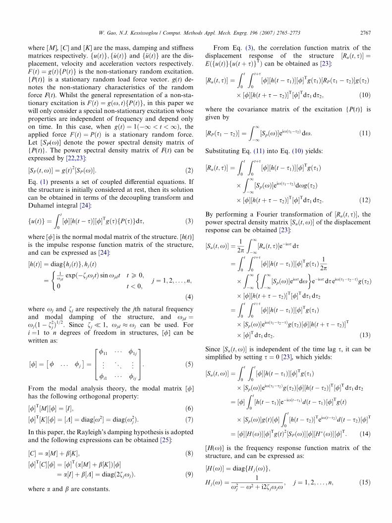
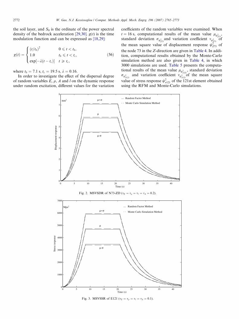
Envelope curves of the mean value (l), mean value plusstandard deviation ðlþ rÞ and mean value minus standarddeviation ðl� rÞ of the mean square value of structuraldisplacement response of the node 73 of Z-direction(MSVSDR of N73-ZD) are shown in Fig. 2. Similar curvesare also presented for the mean square value of structuralstress response of the 121st element (MSVSSR of E121)obtained by using the RFM and Monte-Carlo simulationsare shown in Fig. 3.

From Tables 4 and 5, and in Figs. 2 and 3, it can be seenthat when the variation coefficients of physical parametersare equal to that of geometric dimensions, the randomnessof physical parameters will produce greater effect on therandomness of the mean square value of structural stressresponse, however, the randomness of geometric dimen-sions will produce greater effect on the randomness of themean square value of structural displacement response.

It should be noted that the fact that Monte-Carlo agreeswith the Random Factor method is strongly based uponthe hypothesis on the input data, which is totally correlatedin the current numerical example.

5. Conclusions

In this paper, the randomness of the eth element of atruss structure was considered to be the same for all ele-ments. Then the effect of uncertainty in the material param-eters and structural dimensions on the randomness of thenatural frequencies and mode shapes is presented using anew technique called the Random Factor Method. Theresults from this method are in very good agreement withresults obtained from the Monte-Carlo simulation method.Computational expressions of the mean value, standarddeviation and variation coefficient of the mean squarevalue of the structural displacement and stress responseunder the non-stationary random excitation have also beendeveloped. The dynamic response of the random structureto the stochastic excitation was obtained expediently. Thismethod will also be applied to the non-stationary randomdynamic response analysis of further types of randomstructures.

References

[1] J.T. Oden, T. Belytschko, I. Babuska, T.J.R. Hughes, Researchdirections in computational mechanics, Comput. Methods Appl.Mech. Engrg. 192 (2003) 913–922.

[2] M. Di Paola, A. Pirrotta, M. Zingales, Stochastic dynamics of linearelastic trusses in presence of structural uncertainties (virtual distortionapproach), Prob. Engrg. Mech. 19 (2004) 41–51.

[3] R.S. Langley, Mid and high-frequency vibration analysis of structureswith uncertain properties, in: Proceedings of the Eleventh Interna-tional Congress on Sound and Vibration, St. Petersburg, Russia, 5–8July, 2004.

[4] M. Papadrakakis, A. Kotsopulos, Parallel solution methods forstochastic finite element analysis using Monte Carlo simulation,Comput. Methods Appl. Mech. Engrg. 168 (1999) 305–320.

[5] M. Kaminski, Monte-Carlo simulation of effective conductive forfiber composites, Int. Commun. Heat Mass Transfer 26 (1999) 801–810.

[6] B.N. Singh, D. Yadav, N.G.R. Iyengar, Natural frequencies ofcomposite plates with random material properties using higher-ordershear deformation theory, Int. J. Mech. Sci. 43 (2001) 2193–2214.

[7] M. Kaminski, Perturbation based on stochastic finite element methodhomogenization of two-phase elastic composites, Comput. Struct. 78(2000) 811–826.

[8] K.N. Cho, Mass perturbation influence method for dynamic analysisof offshore structures, Struct. Engrg. Mech. 13 (2002) 429–436.

[9] G. Stefanou, M. Papadrakakis, Stochastic finite element analysis ofshells with combined random material and geometric properties,Comput. Methods Appl. Mech. Engrg. 193 (2004) 139–160.

[10] D. Moens, D. Vandepitte, A survey of non-probabilistic uncertaintytreatment in finite element analysis, Comput. Methods Appl. Mech.Engrg. 194 (2005) 1527–1555.

[11] N.C. Nigam, S. Narayanan, Applications of random vibrations,Narosa, New Delhi, 1994.

[12] D.E. Newland, Random Vibrations, third ed., Wiley, New York,1997.

[13] F.J. Wall, C.G. Bucher, Sensitivity of expected rate of SDOP systemresponse to statistical uncertainties of loading and system parameters,Prob. Engrg. Mech. 2 (1987) 138–146.

[14] W.K. Liu, G. Besterfield, T. Belytschko, Transient probabilisticsystems, Comput. Methods Appl. Mech. Engrg. 67 (1988) 27–54.

[15] H. Jensen, W.D. Iwan, Response of system with uncertain parametersto stochastic excitation, J. Engrg. Mech., ASCE 118 (1992) 1012–1025.

[16] L. Zhao, Q. Chen, Neumann dynamic stochastic finite elementmethod of vibration for structures with stochastic parameters torandom excitation, Comput. Struct. 77 (2000) 651–657.

[17] J.H. Lin, P. Yi, Stationary random response of structures withstochastic parameters, Chinese J. Comput. Mech. 18 (2001) 402–408.

[18] J. Li, S.T. Liao, Dynamic response of linear stochastic structuresunder random excitation, Acta Mech. Sinica 34 (2002) 416–424.

[19] S. Maire, C. De Luigi, Quasi-Monte Carlo quadratures for multi-variate smooth functions, Appl. Numer. Math. 56 (2006) 146–162.

[20] G. Venkiteswaran, M. Junk, Quasi-Monte Carlo algorithms fordiffusion equations in high dimensions, Math. Comput. Simulat. 68(2005) 23–41.

[21] J.C. Helton, F.J. Davis, J.D. Johnson, A comparison of uncertaintyand sensitivity analysis results obtained with random and Latinhypercube sampling, Reliab. Engrg. Syst. Safety 89 (2005) 305–330.

[22] I. Takewaki, Critical envelope functions for non-stationary randomearthquake input, Comput. Struct. 82 (2004) 1671–1683.

[23] C.Y. Yang, Random vibration of structures, John Wiley & Sons, NewYork, 1986.

[24] J.J. Chen, Analysis of engineering structures response to randomwind excitation, Comput. Struct. 51 (1994) 687–693.

[25] W.T. Thomson, M.A. Dahleh, Theory of Vibration with Applica-tions, fifth ed., Prentice-Hall, New Jersey, 1998.

[26] W. Gao, J.J. Chen, Dynamic response analysis of closed loop controlsystem for random intelligent truss structure under random forces,Mech. Syst. Signal Proc. 18 (2004) 947–957.

[27] W. Gao, J.J. Chen, H.B. Ma, X.S. Ma, Optimal placement of activebars in active vibration control for piezoelectric intelligent trussstructures with random parameters, Comput. Struct. 81 (2003) 53–60.

[28] W. Gao, J.J. Chen, M.T. Cui, Y. Cheng, Dynamic response analysisof linear stochastic truss structures under stationary random excita-tion, J. Sound Vibrat. 281 (2005) 311–321.

[29] J.H. Lin, G.Z. Song, Y. Sun, F.W. Williams, Non-stationary randomseismic response of non-uniform beams, Soil Dyn. Earthquake Engrg.14 (1995) 301–306.

[30] I.D. Gupta, M.D. Trifunac, A note on the nonstationarity of seismicresponse of structures, Engrg. Struct. 23 (2000) 1567–1577.

Documents

Dynamic response analysis of stochastic truss structures under non-stationary random excitation using the random factor method