Embed Size (px)
Citation preview

DYNAMIC RESOURCE ALLOCATION
ALGORITHMS FOR COGNITIVE
RADIO SYSTEMS
A THESIS SUBMITTED FOR PARTIAL FULFILLMENT OF THE
REQUIREMENTS FOR THE DEGREE OF
Bachelor of Technology
In
Electronics and Communication Engineering
Under the guidance of Prof. Poonam Singh
Completed by:
Swaraj Rimal (107EC030)
Varun Subramanian (107EC031)
Department of Electronics and Communication Engineering
National Institute of Technology Rourkela
2007-2011

ACKNOWLEDGEMENT
It would not have been possible to complete and write this project thesis without the help
and encouragement of certain people whom we would like to deeply honour and value their
gratefulness.
We would like to highly appreciate the constant motivation and encouragement shown by
our supervisor and guide Prof. Poonam Singh, Department of Electronics and
Communication Engineering during the project and writing of the thesis. Without her
guidance and help, it would not have been possible to bring out this thesis and complete the
project.
We also express our gratitude towards Prof. Sarat Kumar Patra, HOD, Department of
Electronics and Communication, for his selfless support and help offered whenever needed,
especially for the usage of laboratories. Other professors of the department equally have a
space for respect in this thesis for their support. Also, our deep gratitute towards the M.Tech
students and Reasearch scholars who when asked provided with lots of project materials
selflessly.
Last but not the least, our sincere thanks to all the friends who have directly or indirectly
helped us in all the respect regarding the thesis and project. Also, we are indebted to our
institute, NIT Rourkela to have provided the platform for gaining the precious knowledge
and framing the paths of glory for our future.
SWARAJ RIMAL VARUN SUBRAMANIAN
107EC030 107EC031

National Institute of Technology, Rourkela
CERTIFICATE
This is to certify that the thesis entitled “Dynamic Resource Allocation
Algorithms for Cognitive Radio Systems” submitted by Mr. Varun
Subramanian and Mr. Swaraj Rimal for partial fulfilment for the requirement
of Bachelor in Technology degree in Electronics and Communication
Engineering at National Institute of Technology, Rourkela is an authentic piece
of work carried out by them under my guidance and supervision.
To the best of my knowledge, the matter in this thesis has not been
submitted to any other University / Institute for the award of any Degree.
Prof. Poonam Singh
Department of Electronics and Communication
National Institute of Technology, Rourkela
Date:

Table of Contents
1. Abstract ………………………...………………….…………………….…… 1
2. Introduction ……………………………………….…….…………………... 2
2.1. Cognitive Radio
2.2. OFDM for Cognitive Radio
2.3. Objective and Work Done
3. Fair Adaptive Algorithm ………………………………………………..….. 5
3.1. System Model
3.2. Algorithm
3.2.1. Algorithm(MP)
3.2.2. Algorithm(MI)
3.2.3. Algorithm(RC)
3.3. Simulation and Results
3.3.1. Parameters Used
3.3.2. Graphs
4. Max-Min Algorithm ………………………………………………….……. 13
4.1. System Model
4.2. Algorithm
4.3. Simulation and Result
4.3.1. Parameters Used
4.3.2. Graphs
5. Particle Swarm Optimization ………………………………………….... 19
5.1. Introduction
5.2. Parameters of PSO
5.3. The Algorithm

5.4. System Model
5.4.1. System Model with Perfect CSI
5.4.2. System Model with Imperfect CSI
5.5. Allocation Algorithm
5.6. Simulation and Result
5.6.1. Parameters Used
5.6.2. Graphs
6. Genetic Algorithm ……………………………………………………….… 33
6.1. Introduction
6.2. The GA Operators
6.2.1. Selection
6.2.2. Crossover
6.2.3. Mutation
6.3. The Algorithm
6.4. System Model
6.5. Simulation and Result
6.5.1. Parameters Used
6.5.2. Graphs
7. Conclusion…………………………………………….…………………..… 44
8. References…………………………………………….………………..…… 46

1
1. Abstract
Cognitive Radio (CR) is a novel concept for improving the utilization of the radio
spectrum. This promises the efficient use of scarce radio resources. Orthogonal
Frequency Division Multiplexing (OFDM) is a reliable transmission scheme for
Cognitive Radio Systems which provides flexibility in allocating the radio resources in
dynamic environment. It also assures no mutual interference among the CR
radio channels which are just adjacent to each other. Allocation of radio
resources dynamically is a major challenge in cognitive radio systems. In this project,
various algorithms for resource allocation in OFDM based CR systems have been
studied. The algorithms attempt to maximize the total throughput of the CR system
(secondary users) subject to the total power constraint of the CR system and tolerable
interference from and to the licensed band (primary users). We have implemented
two algorithms Particle Swarm Algorithm(PSO) and Genetic Algorithm(GA) and
compared their results.

2
1. Introduction
1.1. Cognitive Radio
With the development of wireless devices and technology, new frequency bands are
being used in the radio spectrum. Due to increase in the wireless device count, the radio
spectrum is becoming increasingly congested. Also, the augmentation in the new wireless
devices with the development in technology has promised more and more frequency band to
be utilized. This may result in the high level of interference among the frequency bands
which are being operated adjacent to each other. Again, it depends on the time and place of
use. However, if trend continues in the future, all the remaining frequency bands will be
utilized and the devices need to face heavy interference thus restricting the performance.
This may lead to deciding of the upper limit to the wireless device count.
Measurements and statistics show that a broad range of the spectrum is not being used
all the time, depending on the geographical region, whereas the other ranges are used
heavily. Thus, the radio spectrum is being underutilized depending on the place and time of
the day. This results in the inefficient use of the spectrum. Generally, the frequency bands
which are licensed operate at fixed time and remaining time they are free. These free or
unused bands of the spectrum cannot be used by conventional wireless systems because
these are licensed and can be used only by the respected owners of that band. So, to use
those bands which are unused by the licensed user during certain time, we need a device
which can automatically change the operating parameters whenever it senses the unused
band.
Cognitive Radio also known as smart radio is an intelligent radio technology which can
learn its radio environments and change its transmission parameters [3]. It was first
proposed by Joseph Mitola in a seminar at KTH, The Royal Institute of Technology, in

3
1998. So, Cognitive Radio is sometimes referred to as Mitola Radio. It can adapt itself to
decide the future actions dynamically to improve the communication quality and meet the
overall requirements of the users. The main feature of CR system is that it is autonomous
and is software controlled. It can change its characteristics dynamically without the
intervention of the user. This involves the sensing of the free spectrum and then deciding the
radio resources such as bandwidth, symbol rate, power, number of subcarriers etc. to a group
of secondary (or CR) users based on the behavior of the users to whom the frequency band
is licensed (primary users). These processes are all controlled by software and are fully
dynamic in nature.
The main functions of Cognitive Radio are to sense the environment, to manage the
environment for data transfer, to look for any disturbances in the environment and if so, then
re-sense the environment for nominal disturbances. It operates in a cycle fashion such that it
begins sensing the environment unless it is not favorable for data transmission. Here,
sensing the environment means sensing the free and unused band of frequency.
The spectrum sensing involves the detection of unused spectrum from the wireless band
which results in minimal interference with other users. The free frequency bands are known
as spectrum holes. There are various techniques by which the spectrum holes can be
detected such as Transmitter detection, Matched Filter detection, Energy detection, etc.
After the proper frequency has been sensed, the problem of spectrum management arrives. It
requires the allocation of various parameters on which data transmission takes place. It
includes allocation of proper subcarriers, transmit power, number of bits per symbol, all
within the interference level of the adjacent band of another user and proper quality of
service. If the operating channel meets with the interference level above threshold, them the
frequency of operation needs to be changed in a smooth manner, not disrupting the existing
data exchange.

4
1.2. OFDM for Cognitive Radio
OFDM stands for Orthogonal Frequency Division Multiplexing. It is the multi-carrier
modulation technique in which data is split up into chunks and every chunk are modulated
using closely spaced orthogonal subcarriers. The orthogonal subcarriers have the property
that they do not have any mutual interference between them. So, this scheme is very useful
for high bit-rate data communication. One of the serious problems of high data rate
transmission is time dispersion of pulses resulting in Inter-symbol Interference (ISI). In
OFDM, the data is split into several low-rate data chunks and are modulated in overlapping
orthogonal subcarriers. These splitting increases the symbol duration by the number of
subcarriers used, thus reducing the ISI due to multipath.
OFDM is adapted as the best transmission scheme for Cognitive Radio systems [3]. The
features and the ability of the OFDM system makes it fit for the CR based transmission
system. OFDM provides spectral efficiency, which is most required for CR system. This is
because the subcarriers are very closely spaced and are overlapping, with no interference.
Another advantage of OFDM is that it is very flexible and adaptive. The subcarriers can be
turned on and off according to the environment and can assist CR system dynamically.
OFDM can be easily implemented using the Fast Fourier Transform (FFT), which can be
done by digital signal processing using software.
1.3. Objective
The main objective of this project is to write optimal algorithms to dynamically
allocate the radio resources to the Cognitive Radio systems which can maximize the
throughput of the system within the power and interference constraints provided by
the alongside operating primary users and total power of the CR system.

5
2. Fair Adaptive algorithm
The Fair Adaptive allocation algorithm is based on the fairness in allocation bit rates for
each secondary user in the CR system. This algorithm is fair in the sense that it tries to
allocate bits to users who have not received their fair share of service as much as possible
[1]. The algorithm first allocates bits to users to ensure fairness, and then subcarrier and
power are decided in greedy manner.
2.1. System Model [1]
We have assumed a system consisting of base station which serves both primary and
secondary users. Let us consider M secondary users are operating in the CR system in the
vicinity of only one primary or licensed user. The primary and secondary users have
adjacent frequency bands. The bandwidth of the primary user band is Wp Hz and that of
secondary sub-band is Ws Hz. We assume the presence of K orthogonal subcarriers such that
K/2 subcarriers are present in either side of the primary band. Hence the total bandwidth of
the CR system is Ws*K/2 Hz. Since orthogonal subcarriers have no interference, only
interference due to primary and secondary users has been considered.

6
The power spectral density (PSD) of kth
subcarrier signal is assumed to be:
( ) (
)
(1)
where,
Pk is the transmit power of kth
subcarrier
Ts is the symbol duration
Let Ik be the interference power introduced by the secondary signal into the primary band.
So,
( ) ∫ | | ( )
(2)
where,
gk is the channel gain from base station to primary user for kth
subcarrier
dk is the spectral distance between kth
subcarrier and primary band
IFk is the interference factor for kth
subcarrier
Let Smk be the interference power introduced by primary signal into kth
secondary band at
mth user. So,
( ) ∫ | | (
)
(3)
where,
hmk is subcarrier k gain from base station to user m
( ) is the PSD of primary user‟s signal
Now, maximum number of bits in a symbol transmitted in the kth
subcarrier is given by:
⌊ ( | |
( ))⌋ (4)
where,
⌊.⌋ denotes the floor function

7
No is the one sided noise PSD
Pmk is the transmit power allocated to kth
subcarrier of mth
user
Γ is set to unity for simplicity
amk є (0,1) is a subcarrier allocation indicator. amk = 1 if kth
subcarrier is allocated to mth
user.
The main objective is to maximize the total bit rate for secondary users constrained by total
transmit power, fairness and interference levels. So, the optimization problem can be
expressed as:
∑∑
where,
amk є {0,1}
∑
∑ ∑
∑ ∑
Ptotal is the total CRU power
Ith is primary user‟s maximum tolerable interference level
The nominal bit rate weight (NBRW) for mth
user is denoted by λm so that (λm / ∑ ) is
the fraction of total secondary user bits loaded to be fairly allocated to user m.
8
2.2. Algorithm [1]
Since the optimal solution for the algorithm is computationally complex and time
consuming, which is not suitable for wireless communication, suboptimal approach have
been used. The algorithm called Reduced Complexity algorithm has been used where a
measure for relative importance of power needed to transmit to secondary users versus
interference power introduced to primary user is determined. Then it is used to determine
which subcarrier to select, having maximum power, or having minimum interference (kp or
ki). First, a minimum power algorithm (MP) is used to determine interference power IMP to
primary user band; we choose the subcarrier which minimizes the incremental power needed
for secondary user. Similarly, minimum interference algorithm (MI) is used to determine
total power PMI required to transmit to secondary users for each bit loading. Subcarrier is
chosen which minimizes the incremental interference power introduced to primary band.
The incremental power required for transmitting one bit to user m on subcarrier k is given
by:
| | (5)
The incremental interference power generated by such a transmission is given by:
(6)
3.2.1. Algorithm (MP)
1) a) P = 0, IMP = 0.
b) Bm = 0 for m = {1, 2,..., M}.
c) bmk = 0 ; calculate ∆Pmk as in (v)
2) a) m* = arg minm Bm/λm
b) kP = arg mink ∆Pm* k

9
c) If (P + ∆Pm*kp < Ptotal), then
Bm* = Bm*+1, P = P+∆Pm*kp,
IMP = IMP + ∆Pm* kp IFkp,
bm*kp = bm*kp + 1, calculate ∆Pm* kp as in (v),
go to step 2a).
d) If (P + ∆Pm*kp > Ptotal), then set m* to be the user with the next higher value of
Bm/λm and go to step 2b). Stop if all users have been considered.
3.2.2. Algorithm (MI)
1) a) PMI = 0, I = 0.
b) Bm = 0 for m = {1, 2,..., M}.
c) bmk = 0 ; calculate ∆Imk as in (vi)
2) a) m* = arg minm Bm/λm
b) kI = arg mink ∆Im* k
c) If (I + ∆Im*kI < Ith), then
Bm* = Bm*+1, I = I+∆Im*kI,
PMI = PMI + ∆Im* kI / IFkI,
bm*kI = bm*kI + 1, calculate ∆Im* kI as in (v),
go to step 2a).
d) If (P + ∆Pm*kp > Ptotal), then set m* to be the user with the next higher value of
Bm/λm and go to step 2b). Stop if all users have been considered.
Now, calculate,
and

10
3.2.3. Algorithm (RC)
1) a) P = 0, I = 0, Bm = 0 for m = {1, 2,..., M}, bmk = 0
b) calculate ∆Pmk as in (v) and ∆Imk as in (vi)
2) a) m* = arg minm Bm/λm
b) kP = arg mink ∆Pm* k
c) kI = arg mink ∆Im* k
d) ( )
,
(
)
e) If (X ≥ Y), set k* = kI ; else set k* = kP
f) If (P + ∆Pm*k* < Ptotal) and (I + ∆Im*k* < Ith) then
Bm* = Bm*+1, P = P+∆Pm*k*, I = I+∆Im*k*
bm*k* = bm*k* + 1, calculate ∆Pm* k* , ∆Im* k*as in (v, vi),
go to step 2a).
g) else, set m* to be the user with the next higher value of Bm/λm and go to step 2b).
Stop if all users have been considered.
Number of bits allocated to secondary users is given by:
∑
The complexity of RC algorithm is O(num_bits x K) where num_bits is the total
number of loaded bits. So, the computation time is not very high.

11
2.3. Simulation and Results
2.3.1. Parameters used
Number of users (M) = 4,
Number of subcarriers (K) = 8
Bandwidth of primary band (Wp) = 0.315 MHz
Bandwidth of secondary band (Ws) = 0.315 MHz,
Symbol rate (Ts) = 4μs,
Noise power (No) = 10-8
W/Hz
All channels are Rayleigh distributed random variables with mean = 1
PSD of primary and secondary signal are same
Total power budget (Ptotal) = 10 W,
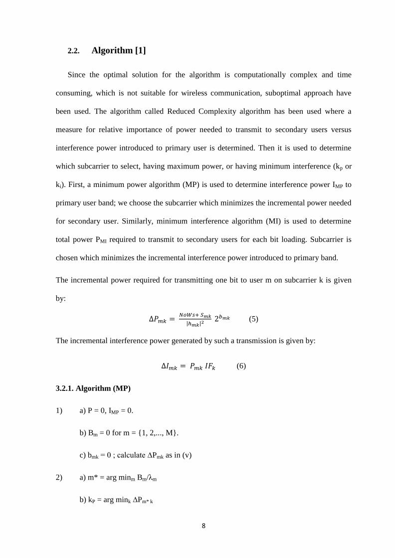
2.3.2. Graphs of maximum bit rate (Rs) v/s Interference threshold (Ith)
Fig. Plot of Rs v/s Ith for different NBRW
12
Fig. Plot of Rs v/s Ith for different CRU power
Fig. Plot of Rs v/s Ith for different Primary power
We observed that as Ith increases, the total bit rate increases till certain value after which
it becomes constant. This is due to the total power constraint provided by the CR system.
After the total power limit is reached, the bit rate ceases to increase and thus becomes
constant. Total data rate can be increased in levels by increasing the CRU power. Bit rate
with no NBRW specified was higher for constant CRU and primary power. As expected,
system with low primary power provided way to increase bit rate in levels as Ith increased.
13
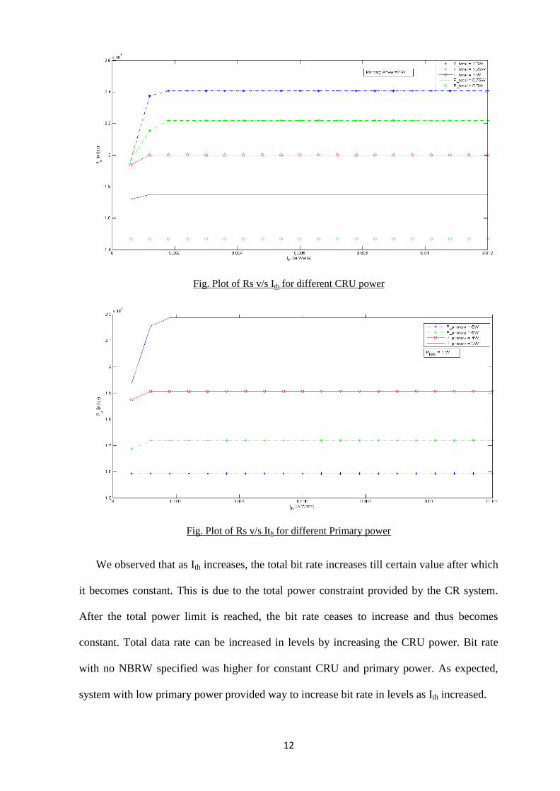
3. Max-Min algorithm
The Max-Min algorithm is based on the greedy approach in allocation of radio resources
while keeping the constraints in power and interference level. In this, we formulate the
optimization as a multidimensional 0-1 knapsack problem and give a low-complexity
solution for this. The fairness among users is not bothered because we consider whole CR
system as a one user.
3.1. System Model [2]
We have assumed a system containing one CR user and three primary users
operating alongside. Since the primary user bands are random in the whole band, the
spectrum holes are generated randomly. The total bandwidth of CRU is W Hz, and M
subcarriers are available in the system. The bandwidth of subcarrier m ranges from [fc + (m
– 1) ∆f] to [fc + m ∆f]. The time varying gain from CRU transmitter to its receiver for each
sub-band m is √ where gm is outcome if independent random variable. There is no
interference among the subcarriers due to orthogonality. The power gains of sub-channel m
from CRU transmitter to PU l‟s receiver and from PU l‟s transmitter to CRU receiver is
denoted by hlm and d
lm respectively. PU l‟s bandwidth ranges from (fc + F
lPU) to (fc + F
lPU +
wl).

14
The interference power generated by PU l to the mth
OFDM sub-channel at the CRU
receiver is:
∫
( )
( ) (
)
( ) (
)
(7)
where ( ) is the PSD of signal of primary user l as in [1].
The number of bits per OFDM symbol, rm, which can be supported for the CRU on
sub-channel m is given by:
⌊ (
( ))⌋ (8)
where
sm is CRU transmission power
σ2 is noise power
Im is interference from PU given by:
∑
(9)
The interference power injected by CRU in subcarrier m into the primary band l is given by:
∫
( )
(
)
(
)
(10)
where ( ) is the base band PSD of the OFDM signal in sub-band m when sm = 1 [1].
The objective is to maximize the overall rate of transmission subject to the specific
thresholds. The problem can be formulated as:
∑ ∑
subject to,

15
∑ ∑
∑ ∑
xn
m є {0,1}
where,
N is the maximum number of bits that can be allocated on any sub-channel and can be set by
the system to any value not exceeding (
) with G = max(gm/σ
2).
( ) is the incremental power required to add the n
th bit to sub-
channel m and xn
m indicates that nth
bit of sub-channel m is allocated. The efficiency
capacity for sub-channel m for constraint l is given by:
(11)
The terms u0 and ul are the costs of resources already allocated, i.e.
∑ ∑
(12)
∑ ∑
(13)
We then greedily allocate a bit to the sub-channel with the largest efficiency value. This
process of allocating one bit at a time is repeated until one of the constraints can no longer
hold.

16
3.2. Algorithm [2]
Initialize ȓm = 0, V m; ul = 0, Vl
while S – u0 > 0 and Ilth – ul > 0, l = 1,2,…..,L
for m = 1 to M
calculate cm (l), Vl using (11)
em = minl {cm(l)}
endfor
α = arg maxm (em)
ȓα = ȓα + 1
update ul, Vl using (12) and (13)
endwhile
The Min-Max algorithm has complexity O(RLM) where R is the total number of allocated
bits.

17
3.3. Simulation and result
3.3.1. Parameters used
All the channel power gains are assumed to be Rayleigh.
Center frequency (fc) = 20MHz
Symbol duration = 4us.
Total bandwidth of the CRU system (W) = 4MHz.
Number of subcarriers = 13
Number of CR users = 1
Number of primary bands = 3
Noise power (σ2) = 10
-8 W.
3.3.2. Graphs for throughput of CR system
For comparison, performance of minimum power algorithm was also plotted.
\Fig. Graph for average no. of bits v/s CRU power

18
Fig. Graph of average no. of bits v/s Ith for each PU
In the first graph the average data rate is plotted versus the total power budget of CR
system keeping the interference threshold constant. The average data rate increased with the
increasing CRU power till the power constraint is maintained, after which it ceased to
increase and became constant. The upper limit of the total power is kept in the sense that the
power of CR system above that will cause signal spill to the primary band and thus results in
interference, causing the data rate to become constant. In the second graph, the average data
rate is plotted versus the interference threshold for constant power of CR system. We found
that the data rate increases on increasing threshold because there is still some room for
enough interference to occur. The data rate became constant when upper limit in
interference threshold was reached because of the total power constraint of the system.
MP algorithm performed poorly against Max-Min algorithm. For every simulation, the
MP results were degraded in comparison with the Max-Min algorithm.

19
4. Particle Swarm Optimization (PSO)
4.1. Introduction
The Particle Swarm Optimization (PSO) is a swarm intelligence-based evolutionary
algorithm. It is a biologically inspired algorithm motivated by social analogy. Its aim is to
obtain the global optimum of a real-valued function defined in a given space [8]. It was
inspired by the behavior of the swarm to look for food. This was introduced first by
Kennedy and Eberhart in the year 1995. Kennedy was an American psychologist and
Eberhart was an electrical engineer. This algorithm makes use of social behavior and
movement dynamics of insects, birds and fish. Let us take example of the fish food
searching behavior. The searching space of the fish can be considered as the search space
and the fish in the shoal can be considered as small particles denoting solutions in the search
space. The process of searching the food can be viewed as an optimization process. In the
process, the members of the shoal compete among themselves and share the information
with the partners to find the best solution of the problem altogether.
The research have shown that when birds or fishes search for food, they do it in groups
(flocks or swarms) and not individually. The observation is based on the assumption that the
information is shared inside the group among the individuals. The behavior of each
individual is influenced by the behavior of the whole group. The PSO was developed
through simulation of the simplified social system and has been found robust in solving non-
linear optimization problems [7]. The PSO algorithm can produce simplified and good
solution with lesser calculations, shorter time and stable convergence than any other
conventional methods.

20
The PSO is closely related to the Artificial Life and Evolutionary Algorithms. It uses a
position-velocity model in a swarm based searching process. A swarm consists of a set of
individuals or particles, each representing a potential „solution‟ of the problem being
formulated. Each particle is characterized by its position and velocity in the searching space.
The position and velocity determine the searching region. The fitness value for each particle
is evaluated by using the position and velocity to determine the solution performance using
the avail or the fitness function.
There are various pros and cons of the PSO algorithm which makes it limited in use in
certain areas only. It has very efficient global search algorithm and is easy to implement
with less number of parameters to be determined. However, it has slow convergence in the
refined search stage or has weak local search ability. But still it is simple to use and is
immune to the changing the scale of the parameters.
The PSO algorithm is best suited to the continuous variable problems. It has been
applied to a number of applications including the Artificial Neural Networks. It is used in
the training of Neural Networks in areas like image processing and Fuzzy logic. It can be
applied in electrical distribution field for optimized power supply. Various other
applications include system identification in biomechanics and biochemistry and in
structural optimization of shape and size design.
Two basic types of PSO can be identified based on the processing of the algorithm,
synchronous and asynchronous PSO. In synchronous PSO the particles are evaluated
parallel first and then they are compared. Generally, a synchronous point is required for all
the particles from where again the process can start for iteration. In asynchronous PSO, each
particle is evaluated separately and then compared in every step. If a particle is already
found to be fit, it need not be re-evaluated, thus saving the computation time.

21
4.2. Parameters of PSO [7]
1. Initial Population: The population is the set of n particles, and is generated
randomly.
2. Population Size: It refers to the number of particles in a swarm and should be set
according to the problem (based on the tradeoff between accuracy and computation
time).
3. Swarm: It is a set or group of the particles or population which move in random
directions.
4. Search Space: It is the range in which the algorithm computes the solution. It is the
set of solutions defined in a space.
5. Number of Iterations: It refers to the maximum number of steps required for the
fitness value to converge to an optimal solution.
6. Inertia weight: The inertia weight controls the convergence of the algorithm and
should be chosen very carefully. Too high or too low inertia weight can lead
convergence to fail and no solution will be obtained.

22
4.3. The Algorithm
The position and velocity of the particles are randomly initialized based on the searching
technique. The position of a particle i is denoted as xi,k and its velocity by vi,k , k being the
iteration number. So, the position and velocity can be denoted in vector form by Xi=[xi,1,
xi,2, xi,3…..xi,k] and Vi=[vi,1, vi,2, vi,3…….vi,k]. An avail function (fitness function) is evaluated
for a particle at each iteration using the position and velocity to find out the best solutions.
The solution for each particle is then stored in Pbest. This is known as best local solution and
is the best solution it has achieved so far in the iteration. The fitness value is also stored.
After all iteration, the best solution for whole swarm is found out as Gbest.
The position and velocity is updated as the following equations:
xi,k+1 = xi,k + vi,k+1 (14)
vi,k+1 = ωvi,k + c1r1(Pbest – xi,k) + c2r2(Gbest – xi,k) (15)
where,
ω is the inertia weight
c1, c2 are positive accelerators
r1, r2 are random numbers
Parameters c1 and c2 are constant values. Low values allow the particles to roam far
from the target values, whereas the high values result in abrupt movements towards the
target values. Normally, their values are set to be 2. The random values of r1 and r2 are
uniformly distributed between zero and one, [0, 1]. To restrict the searching space, the
maximum and minimum values of the velocity and position are defined as [Vmax, Vmin] and

23
[Xmax and Xmin]. The above equations enable the particles to evaluate themselves and update
the position and velocity every time to find the optimum for the swarm.
The following steps are involved in the PSO operation:
1. Initialization: The position and velocity of the particles are randomly initialized.
2. Evaluation: The particles are evaluated by calculating their respective avail
function. The current position and the avail values are stored in the Pbest of each
particle. The best position of whole swarm is stored in Gbest.
3. Updation: The position and velocity of particles are updated according to the
equations (14) and (15). The particles are again evaluated by their avail values. If the
avail value of the updated particle is greater than the current particle, the Pbest value
is replaced by the updated position. Then, Gbest is updated after all the iteration.
4. Termination: When the maximum number of iterations is over or when the stopping
criteria are met, Gbest is the optimal solution. Or else, go to step 3.
24
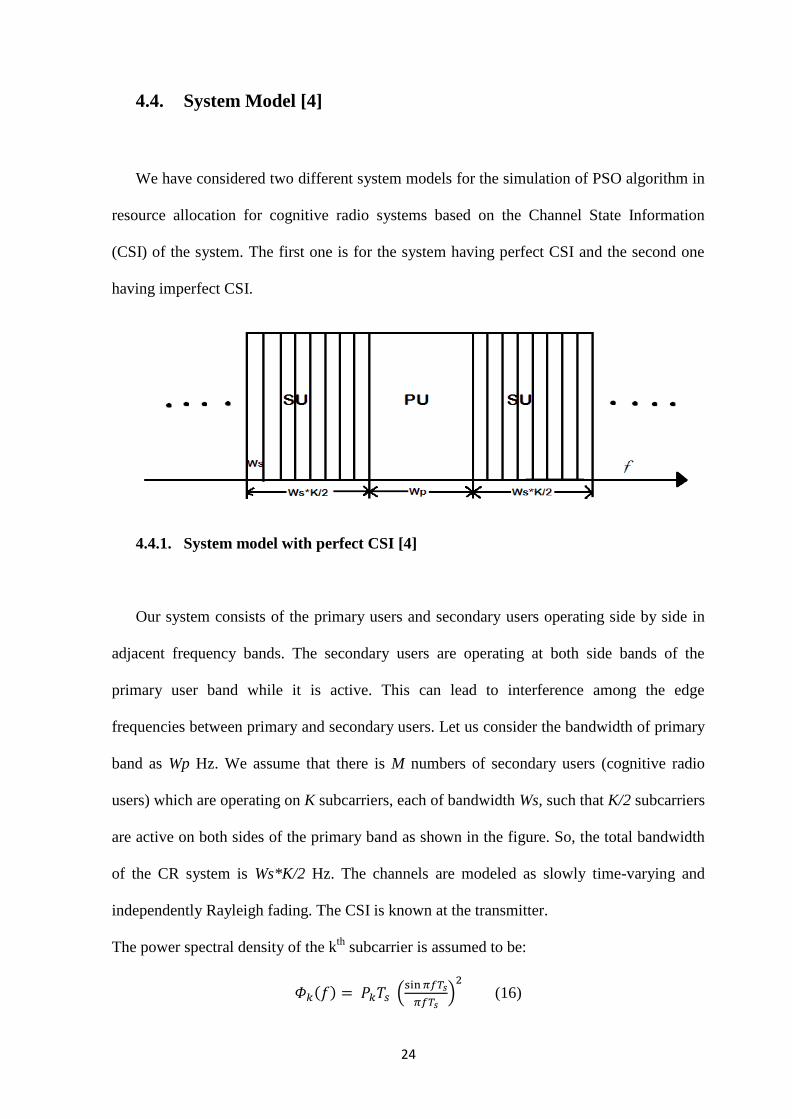
4.4. System Model [4]
We have considered two different system models for the simulation of PSO algorithm in
resource allocation for cognitive radio systems based on the Channel State Information
(CSI) of the system. The first one is for the system having perfect CSI and the second one
having imperfect CSI.
4.4.1. System model with perfect CSI [4]
Our system consists of the primary users and secondary users operating side by side in
adjacent frequency bands. The secondary users are operating at both side bands of the
primary user band while it is active. This can lead to interference among the edge
frequencies between primary and secondary users. Let us consider the bandwidth of primary
band as Wp Hz. We assume that there is M numbers of secondary users (cognitive radio
users) which are operating on K subcarriers, each of bandwidth Ws, such that K/2 subcarriers
are active on both sides of the primary band as shown in the figure. So, the total bandwidth
of the CR system is Ws*K/2 Hz. The channels are modeled as slowly time-varying and
independently Rayleigh fading. The CSI is known at the transmitter.
The power spectral density of the kth
subcarrier is assumed to be:
( ) (
)
(16)

25
where,
Pk is the transmit power of kth
subcarrier
Ts is the symbol duration
Let Ik be the interference power introduced by the secondary signal into the primary band.
So,
( ) ∫ | | ( )
(17)
where,
hk is the channel gain for kth
subcarrier
dk is the spectral distance between kth
subcarrier and primary band
IFk is the interference factor for kth
subcarrier
Let Smk be the interference power introduced by primary signal into kth
secondary band
( ) ∫ | | (
)
(18)
where,
hmk is the channel gain for kth
subcarrier for mth user
( ) is the PSD of primary user‟s signal
We formulate the constraint that:
∑ ( )
where,
Ith is the interference threshold constraint decided by the PU

26
According to [4] and [5], we can write the expression for the power allocated to each
subcarrier k as:
∑
| |
| |
(19)
where,
σ2
is the noise variance
Now, with the power and bits allocated to the subcarriers, the data rate of a
subcarrier can be denoted as:
( ) ( | |
( )
)
(20)
4.4.2. System model with imperfect CSI [11]
The system model for the resource allocation of CR system with imperfect Channel
State Information is same as that of with perfect CSI given above. All the equations for
PSD, the power level, interference, data rate and bits per symbol remain same. The previous
model was based on the assumption that the transmitter had the true estimation of the
channel i.e. there was a full information about channel gain at the transmitter. But, however
in practical wireless applications, having a true estimate of channel at the transmitter is not
possible and some estimate of the channel has to be made out of statistics, which of course
deviates from the true estimate of the existing channel. So, there will be degradation in the
overall system performance as compared to the system having perfect CSI.
As previous model, we assume that there is M numbers of secondary users (cognitive
radio users) which are operating on K subcarriers, each of bandwidth Ws, such that K/2
subcarriers are active on both sides of the primary band. In this system model, we have
assumed that the transmitter has imperfect or partial Channel State Information, and the

27
channel undergoes an independently Rayleigh fading. We implement PSO for the resource
allocation based on the system model.
The channel estimation with imperfect information at the transmitter can be formulated
as the sum of the true estimation of channel and estimation error. Let h denote the actual
channel gain, which can be referred either from the CR base station to the kth
subcarrier of
mth
user or to the primary user. The estimated channel gain is given by:
(21)
where,
e is the channel estimation error
For simplicity and simulation reasons, e is assumed to be an outcome of
independent, circularly symmetric Gaussian random variable.
The maximum bit rate for a subcarrier per user, Rmk, depends on the channel gain
hmk, transmit power Pmk and interference levels. But in this case, the transmitter does not
know hmk, instead, it has the information about the estimation mk. Therefore, the algorithm
calculates the estimated version of bit rate, mk. Two conditions arise in this case. If mk <
Rmk, then the higher bit rate cannot be achieved, and if mk > Rmk, then it exceeds the
channel capacity and the total bit rate will be zero. So overall, the maximum bit rate of the
system, Rs with imperfect channel estimation will always be less than that of system with
true channel estimation.
To reduce the overall throughput degradation due to inaccurate channel gain, a back-off
factor BG has been introduced such that 0 ≤ BG ≤ 1. This factor is multiplied to the channel
gain in order to stabilize it and thus normalizing the gain so that there is no extreme change
in the gain. So we replace the channel gain hmk in all the equations with BG* mk and all
other steps in algorithm are the same.

28
4.5. Allocation Algorithm
The maximum number of bits per symbol to be loaded on a subcarrier for any user m can
be written as:
⌊ ( | |
( )
)⌋
(22)
where,
Pmk is the power allocated to subcarrier k of user m
⌊.⌋ is the floor function
Now, the main objective of our algorithm is to maximize the total data rate Rs of
the secondary users (of the whole CR system) constrained to the maximum level of
interference to primary users and maximum allowable transmit power for every
subcarrier. The maximum achievable bit rate is given as:
∑∑
And the interference constraint is formulated as:
∑∑ ( )
As for PSO, the avail function or the fitness function can be written as:
( ) (∑ ∑ ( )
)
(23)
where,
A(Rs, Imk) is the avail value achieved by allocating power and bits to users
is the coefficient as a tradeoff between data rate and interference to PU
29
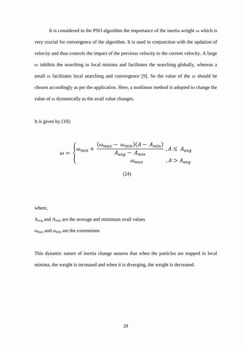
It is considered in the PSO algorithm the importance of the inertia weight ω which is
very crucial for convergence of the algorithm. It is used in conjunction with the updation of
velocity and thus controls the impact of the previous velocity to the current velocity. A large
ω inhibits the searching in local minima and facilitates the searching globally, whereas a
small ω facilitates local searching and convergence [9]. So the value of the ω should be
chosen accordingly as per the application. Here, a nonlinear method is adopted to change the
value of ω dynamically as the avail value changes.
It is given by [10]:
{
( )( )
(24)
where,
Aavg and Amin are the average and minimum avail values
ωmax and ωmin are the extremisms
This dynamic nature of inertia change assures that when the particles are trapped in local
minima, the weight is increased and when it is diverging, the weight is decreased.

30
4.6. Simulation and Results
4.6.1. Parameters used:
System Model:
Number of users (M) = 4
Number of subcarriers (K) = 16
Center frequency (f) = 2 GHz
Bandwidth of Primary band (Wp) = 5 MHz
Bandwidth of subcarrier (Ws) = 312.5 KHz
Symbol rate (Ts) = 4 μs
Noise power (σ2) = 10
-8 W
Channel is independently Rayleigh fading
PSD of primary and secondary signal are same
Back-off factor (BG) = 0.84
PSO Algorithm:
Number of particles = 1000
Number of iterations = 25
Tradeoff coefficient (χ) = 100
Positive accelerator 1 (c1) = 2
Positive accelerator 2 (c2) = 2
Minimum inertial weight (ωmin) = 0.4
Maximum inertial weight (ωmax) = 0.9
Maximum velocity (Vmax) = 0.2 * (Xmax – Xmin), X is the position
Minimum velocity (Vmin) = -Vmax
The algorithm was run for 25 realizations and then results were averaged out

31
Separate simulations were carried out for system with perfect CSI and system with
imperfect CSI. Also, a comparison was carried out between the two and was plotted in the
graph. The graph was plotted for maximum data rate of the system (Rs) versus the
Interference threshold (Ith) of the system as prescribed by the primary user.
4.6.2. Graphs for throughput of CR system
Fig: Plot of data rate versus interference threshold for Perfect and Imperfect CSI using PSO (Primary
power = 3 W)
Fig: Plot of data rate versus interference threshold for Perfect and Imperfect CSI using PSO (Primary
power = 4 W)

32
Fig: Plot of data rate versus interference threshold Imperfect CSI using PSO for various Ppu
The first graph represents the plot of total data rate (Rs) versus the Interference
Threshold (Ith) constraint provided by the primary user. The power of the primary user
system is assumed to be 3 Watts. We can find out from the graph that the total data rate
increases for increasing value of the interference threshold as more and more number of bits
can be loaded in the subcarriers with no interference. After reaching the interference limit,
the data rate stops increasing and becomes constant.
The second graph represents the plot of total data rate (Rs) versus the Interference
Threshold (Ith) constraint provided by the primary user. The power of the primary user
system is assumed to be 4 Watts. Here also, the total data rate increases for increasing value
of the interference threshold till the constrained is reached. By comparing the above two
graphs, we find out that the data rate in the system with less primary power is higher than
the system with high primary power. This is due to the fact that interference is more easily
encountered in system with high power, thus reducing the data rate. The system with
imperfect CSI has poorer performance then the system with perfect CSI due to obvious
reasons. However, the practical wireless system always has the imperfect CSI to the
transmitter, hence is the true performance of the practical system.
33
5. Genetic Algorithm
5.1. Introduction
Genetic Algorithm (GA) is another biologically (genetically) inspired evolutionary
algorithm used to solve complex computational problems to find optimal solutions. It is
fully based on biological model of solving problems through various genetic techniques. It
uses the principles of selection and evolution to produce several solutions to a given
problem [16]. IT is based on the genetic process of many organisms. By mimicking the
principle of natural selection and process of survival of the fittest, as given by Charles
Darwin in his book, The Origin of Species, this algorithm is able to evolve the solutions to
the real world problems [18]. This algorithm was first introduced and investigated by John
Holland and his students in the year 1975. The GA encodes the potential solution into a
specific problem on a simple chromosome- like data structure and applies recombination
operators to these structures so as to preserve the critical information.
Like PSO, the Genetic Algorithm also has random population, this time the
chromosomes, in the search space which represent the solutions for the problem. The
difference being that GA produces new set of population in the solution space as fit
individuals. The implementation of Genetic Algorithm begins with the population of random
chromosomes. These chromosomes are then evaluated and fittest chromosomes are given
reproductive opportunities so as to produce a better set of other chromosomes, which
represents better solution. Any set of population are defined better as compared to the
current set of population [17].

34
This algorithm generally thrives in the environment which has a very large set of
candidate solutions and in which the search space is uneven and has many hills and valleys.
The basic Genetic Algorithm works as described. First, a population (set of chromosomes) is
created randomly. Then, each chromosome in the population is evaluated individually based
on some fitness function. The fitness function can be anything, as set by the programmer
based on the problem and application. Each individual is given a score after the evaluation
of how well they have performed. Then, based on the score, two individuals are selected.
This selection is completely based on the ranking of the individuals, higher the rank, more
the chance of being selected. The selected two individuals are then reproduced to produce
one or more offspring. The whole idea is to produce best reproduced individuals from fittest
parents. The offspring are then mutated randomly using some method to add to its existing
characteristics. This process is continued until the required optimal solution has been found
or certain generations have passed. So, the solutions get better and optimal as the
generations go by. The GA processes populations of chromosomes, successively replacing
one such population with another.
Before performing the GA operation, appropriate coding must be done to the problem.
One of the most common forms of coding technique is the binary coding. In this, the
chromosome, or the individual of the population is represented using large strands of 0s and
1s. Each value or parameters of a strand is known as genes. The most important part while
performing GA is the fitness function. The fitness function of an individual returns a single
numerical value proportional to the ability of the individual which that chromosome
represents.

35
5.2. The GA Operations
Three types of operators generally are handled in simplest kind of Genetic Algorithm.
These are: selection, crossover and mutation.
5.2.1. Selection
As discussed above, the individuals are picked up from the population in
order to reproduce. The individuals are selected on the basis of their fitness
value. Several techniques are there to select the individuals, out of which the
roulette wheel selection is the most common. In roulette wheel selection,
individuals are given a probability of being selected that is directly
proportionate to their fitness value. Two individuals are then chosen randomly
based on these probabilities and produce offspring. The fitter the chromosome,
the more times it is likely to be selected to reproduce.
5.2.2. Crossover
Crossover is the form of reproduction between two individuals. Generally, a
single point crossover is used. In this method two individual chromosomes are
taken and a random point is chosen along the strands from where each individual
chromosome is cut into two segments. These segments are referred to as head
segments and tail segments. The tail segments are then swapped between two
individuals thus producing the two new individuals and are added to the
population. Since only one point is chosen in each chromosome to crossover, it
is known as single-point crossover. For example, the strings 10000100 and
11111111 could be crossed over to produce the two offspring 10011111 and
11100100. Here, the crossover point is the 4th
gene in each strand. The crossover
operation roughly mimics biological recombination between two single
36
chromosome organisms. Crossover does not necessarily always occur, however.
Sometimes, based on a set probability, no crossover occurs and the parents are
copied directly to the new population. The probability of crossover occurring is
usually 60% to 70%.
5.2.3. Mutation
After the crossover, the new chromosomes are added to the populations, or
not necessarily this happens, in which case the parents are directly copied and
kept into the population. So, to ensure the uniqueness of individuals in the
population, mutation is performed for certain individuals. In mutation, where
binary encoded chromosomes are used, some of the bits in a chromosome are
randomly flipped, making them unique in the population. For example, the
string 00000100 might be mutated in its second position to yield 01000100.
Mutation can occur at each bit position in a string with some probability,
usually very small (e.g., 0.001). Mutation is, however, vital to ensuring genetic
diversity within the population.
5.3. The Algorithm
A simple Genetic Algorithm works as follows, if given a clearly defined problem to be
solved and a bit string representation for candidate solutions.
1. A population of n, l-bit chromosomes is randomly generated, which are the candidate
solutions to the given problem.
2. Each chromosome is evaluated using the fitness function and a fitness value is
assigned to each one of them.
3. The following steps are repeated until n offspring have been created:

37
a. A pair of parent chromosomes is selected form the current population with
the probability of selection being an increasing function of fitness. That is,
the two fittest chromosomes are taken as a pair. The selection is done with
replacement, which means that the same chromosome can be selected more
than once to become a parent.
b. The pair is then crossed over at some randomly chosen point, chosen with
uniform probability. It is done with some probability, which is known as the
crossover probability or crossover rate. If no crossover takes place, two
offspring are formed that are exact copies of their parents.
c. The two new offspring are then mutated at some random point with some
probability, known as mutation probability or mutation rate. Then the
resulting chromosomes are placed in the new population.
If n is odd, then one new chromosome can be discarded at random.
4. The current population is replaced with the new population.
5. Go to step 2 and continue until optimal solutions are obtained or desired number of
generations is reached.
Each iteration of this process is called a generation. A GA is typically iterated for
anywhere from 50 to 500 or more generations. The entire set of generations is called a
run. At the end of a run there are often one or more highly fit chromosomes in the
population. Since randomness plays a large role in each run, two runs with different
random−number seeds will generally produce different detailed behaviors.

38
5.4. System Model [4]
The system model used to perform Genetic Algorithm is same as that used for PSO.
Our system consists of the primary users and secondary users operating side by side
in adjacent frequency bands. The secondary users are operating at both side bands of the
primary user band while it is active. The bandwidth of primary band is Wp Hz and that of
one secondary subcarrier is Ws Hz. M users are operating on K subcarriers. So, Ws*K/2 Hz
of subcarriers are operating at each side of the primary band.
In this case also, we have considered the case of system with perfect and imperfect
Channel State Information. First the system where the transmitter has the true channel
information is considered and simulated. Then the results are compared to the one having
imperfect channel information. The equations, power and interference constraints, the data
rate equations and the fitness function all are same as considered for the case of PSO. So,
we are using two different algorithms for resource allocation in the same CR system, and
also comparing the performance of both algorithms.
Like for PSO, the fitness function can be written as:
( ) (∑ ∑ ( )
)
where the letters and symbols have their usual meanings. (Refer to section 5.4 and 5.5)

39
5.5. Simulation and Result
5.5.1. Parameters used:
System Model:
Number of users (M) = 4
Number of subcarriers (K) = 16
Center frequency (f) = 2 GHz
Bandwidth of Primary band (Wp) = 5 MHz
Bandwidth of subcarrier (Ws) = 312.5 KHz
Symbol rate (Ts) = 4 μs
Noise power (σ2) = 10
-8 W
Channel is independently Rayleigh fading
Back-off factor (BG) = 0.84
Genetic Algorithm:
Number of chromosomes = 20
Number of generations = 40
The algorithm was run for 25 realizations and then results were averaged out

40
5.5.2. Graphs for throughput of CR system
Fig: Plot of data rate versus interference threshold for GA with various primary power
Fig: Plot of data rate versus interference threshold for Perfect and Imperfect CSI GA
with primary power = 3W

41
Fig: Plot of data rate versus interference threshold for Perfect and Imperfect CSI using
GA (Primary power = 4 W)
Fig: Plot of data rate versus interference threshold for PSO and GA in perfect CSI
(Primary power = 1W)

42
Fig: Plot of data rate versus interference threshold for PSO and GA in imperfect CSI
(Primary power = 1W)
The first graph is the performance of Genetic Algorithm under perfect CSI for
various primary power levels. As the power of primary system increases, the data rate
decreases in levels as interference increases. This is plotted against increasing interference
threshold as provided by the primary system.
The next two graphs are the comparison of performance of Genetic Algorithm for
different primary power and under perfect and imperfect CSI. These graphs represent the
plot of total data rate (Rs) versus the Interference Threshold (Ith) constraint provided by the
primary user. The power of the primary user system is assumed to be 3 Watts in first graph
and 4 Watts in second graph. We can find out from the graph that the total data rate
increases for increasing value of the interference threshold as more and more number of bits
can be loaded in the subcarriers with no interference. After reaching the interference limit,
the data rate stops increasing and becomes constant. However, the performance of the
system with imperfect Channel State Information is inferior as compared to the system with
perfect CSI. Again, system with imperfect CSI is practical among the wireless systems. The
43
system with low primary power has higher data rate whereas the system with high primary
power has low data rate for interference issues.
The last two graphs are the comparisons between PSO and GA for perfect and imperfect
CSI for primary power of 1 Watt. We can see that both algorithms have similar
performances as they both produce optimal solutions for the problem. However, GA is
inferior to PSO in the sense that more computational time is required for GA and is slow
compared to PSO. This is due to many operations required for GA. Therefore, PSO is
preferred over GA for similar type of applications.

44
6. Conclusion
Hence, various sub-optimal and optimal algorithms were studied and implemented for
the purpose of dynamically allocating the resources for the Cognitive Radio Systems. Some
algorithms were directly implemented from certain papers, which are the work done by
esteemed engineers, and simply their behavior was studied. First, a low-complex Fair
Adaptive algorithm was implemented from [1]. We used the system model where a primary
band was operating side by side to the secondary band in a multi user system. So,
interference issues had to be taken care of. Sub-optimal approach was used to simulate the
behavior of the throughput of the system as Reduced Complexity (RC) algorithm. It
allocates the resources to users in a fair manner, without any power or bits favor to any
particular user. The second algorithm we implemented was Max-Min Algorithm [2]. It used
the greedy approach to allocate resources to the user. Only one CR user was considered and
three primary users were operating side by side. We formulated the optimization as a
multidimensional 0-1 knapsack problem and provided a low-complex and sub-optimal
solution for this.
Then we studied and implemented Particle Swarm Optimization (PSO), which provides
with low-complex optimal solution. Its performance was far better than the previous
algorithms. We used the system model of [4] where a primary band is operating side by side
to the multi-user CR system. We simulated the PSO for two types of system, one where the
transmitter has full information about the channel state and the other where the transmitter
has only partial information about the channel. The first case is referred to as system with
perfect CSI and the second as imperfect CSI. The system with imperfect CSI is the most
practical wireless system where true estimation of channel cannot be done. As expected, the
performance of imperfect CSI system was inferior compared to that of having perfect CSI.

45
Last, we studied and implemented Genetic Algorithm, which, like PSO, provides the
most optimal solution for the complex problems. Hence this algorithm can be comparable to
the PSO. Again, the same system model was used as [4] and the algorithm was simulated for
two types of system, one having perfect CSI and another having imperfect CSI. The
performance of the system with this algorithm was comparable to the PSO, the difference
being in only the computational time where GA took more time in producing the solutions.
This is based on the fact that GA requires more operations to perform than PSO and hence
takes longer time.
So, we conclude that Particle Swarm Optimization algorithm is best suited for dynamic
resource allocation in Cognitive Radio Systems where the resources are allocated in a
dynamic environment within the given constraints of power and interference in a very
optimal manner.

46
7. References
[1]. Tao Qin and Cyril Young, “Fair Adaptive Resource Allocation for Multiuser OFDM
Cognitive Radio Systems”, Wireless Communications, IEEE Transactions, Volume: 4 Issue:6 page(s): 2726 – 2737.
[2]. Yonghong Zhang and Cyril Leung, “Resource Allocation in an OFDM Based Cognitive
Radio System”, IEEE Journal on IEEE Transactions on Communications, Vol.57, No.7,
July 2009
[3]. Hisham a Mahmoud, Tevfik Yücek, and Hüseyin Arslan, University of South Florida,
“OFDM for Cognitive Radio: Merits and Challenges”, IEEE Wireless Communications,
April 2009, Volume: 16 Issue:2 Pages 6-15.
[4]. Shiquan Xu, Qinyu Zhang and Wei Lin, “PSO-Based OFDM Adaptive Power and Bit
Allocation for Multiuser Cognitive Radio System”, IEEE Journal, Issue Date: 24-26 Sept.
2009 page(s): 1 - 4
[5]. G. Bansal, J. Hossain and V. K. Bhargava, “Adaptive Power Loading for OFDM-based
Cognitive Radio Systems,” in Proc. of IEEE International Conference on
Communications. ICC‟07, 24-28 June 2007, pp. 5137-5142
[6]. Jaco F. Schutte, “The Particle Swarm Optimization Algorithm”, EGM 6365-Structural
Optimization, Fall 2005
[7]. Prabha Umapathy, C. Venkataseshaiah, and M. Senthil Arumugam, “Particle Swarm
Optimization with Various Inertia Weight Variants for Optimal Power Flow Solution”,
Discrete Dynamics in Nature and Society, Volume 2010 (2010), Article ID 462145
[8]. J. Kennedy, R.C. Eberhart, and Y. Shi, “Swarm intelligence”, Morgan Kaufmann
Publishers, San Francisco, 2001.
[9]. R. C. Eberhart, and Y. Shi, “A modified particle swarm optimizer,” in Proc. of the IEEE
CEC. 1998: 69-73
[10]. L. Wang, and B, Liu, “Particle Swarm Optimization and Scheduling Algorithms,”
Beijing Tsinghua University, 2008, ISBN: 978-1-4244-3692-7

47
[11]. Tao Qin, Cyril Leung, Chunyan Miao, and Zhiqi Shen, “Resource Allocation in a
Cognitive Radio System with Imperfect Channel State Estimation,” Journal of Electrical
and Computer Engineering, vol. 2010, Article ID 419430, 5 pages, 2010.
doi:10.1155/2010/419430
[12]. Yonghong Zhang, Cyril Leung: A Distributed Algorithm for Resource Allocation in
OFDM Cognitive Radio Systems. VTC Fall 2008: 1-5
[13]. Muhammad Waheed and Anni Cai, “Evolutionary Algorithms for Radio Resource
Management in Cognitive Radio Network”, Performance Computing and Communications
Conference (IPCCC), 2009, 14-16 Dec. 2009, page(s): 431, ISSN: 1097-2641, Print
ISBN: 978-1-4244-5737-3
[14]. Mindi Yuan, Shaowei Wang and Sidan Du, “Fast Genetic Algorithm for Bits
Allocation in OFDM Based Cognitive Radio Systems”, Wireless and Optical
Communications Conference (WOCC), 2010 19th Annual, Issue Date : 14-15 May 2010
page(s): 1 ISBN: 978-1-4244-7597-1
[15]. John Kennedy, Russel Eberhart, “Particle Swarm Optimization”, From Proc. IEEE Int'l.
Conf. on Neural Networks (Perth, Australia), IEEE Service Center, Piscataway, NJ,
IV:1942-1948.
[16]. Michael Skinner, “Genetic Algorithms Overview”
[17]. Darrel Whitley, “A Genetic Algorithm Tutorial”
[18]. David Beasley, David R. Bull and Ralph R. Martin, “An Overview of Genetic Algorithms:
Part 1 , Fundamentals”, University Computing 1993, Inter-University Committee on
Computing
[19]. http://www.hindawi.com/journals/ddns/2010/462145/
[20]. http://tracer.uc3m.es/tws/pso/basics.html
[21]. http://www.swarmintelligence.org/tutorials.php
[22]. http://www.engr.iupui.edu/~shi/Coference/psopap4.html
[23]. http://geneticalgorithms.ai-depot.com/Tutorial/Overview.html