Dynamic Programming Approximations for Stochastic,Time-Staged Integer Multicommodity Flow Problems

Huseyin TopalogluSchool of Operations Research and Industrial Engineering,

Cornell University, Ithaca, NY 14853, USA, topaloglu@orie.cornell.edu

Warren B. PowellDepartment of Operations Research and Financial Engineering,

Princeton University, Princeton, NJ 08544, USA, powell@princeton.edu

In this paper, we consider a stochastic and time dependent version of the min-cost integer multi-commodity flow problem that arises in the dynamic resource allocation context. In this problemclass, tasks arriving over time have to be covered by a set of indivisible and reusable resources ofdifferent types. The assignment of a resource to a task removes the task from the system, modifiesthe resource, and generates a profit. When serving a task, resources of different types can serve assubstitutes of each other, possibly yielding different revenues. We propose an iterative, adaptivedynamic programming-based methodology that makes use of linear and/or nonlinear approxima-tions of the value function. Our numerical work shows that the proposed method provides highquality solutions and is computationally attractive for large problems.

Key words: dynamic programming; networks-graphs; multicommodity; transportation.History: received August 2003; revised February 2004.

1. Introduction

Dynamic resource allocation problems involve the assignment of a set of reusable resources to

tasks that occur over time. The arrival process of the tasks is known only through a probability

distribution. The assignment of a resource to a task produces a reward, removes the task from

the system and modifies the state of the resource. Such problems arise in many fields such as

dynamic fleet management, product distribution, machine scheduling and personnel management.

In this paper, we consider dynamic resource allocation problems in which there is substitution

among resources. Different types of resources can be used to cover a task, and covering a task with

different types of resources may yield different rewards.

We were confronted with this problem within the context of managing a fleet of business jets

to serve customers that request to be flown between different airports. The fleet is composed

of different types of jets. Due to operating costs and customer preferences, satisfying a certain

customer demand with different types of jets yields different revenues. Given the high repositioning

costs and substitution penalties, effective repositioning of the available jets in order to serve the

1

uncertain future customer requests and using the “correct” type of jet to satisfy a demand are

crucial. Clearly, very often the jet type that maximizes the immediate profit is not necessarily the

best pick.

The deterministic version of this problem is the min-cost integer multicommodity flow problem.

The linear and integer versions of the min-cost multicommodity flow problem have been studied

extensively. Early survey papers by Assad (1978) and Kennington (1978) describe various solution

approaches to the linear version. The integer version has seen increased attention due to its wide ap-

plicability to fields such as airline fleet assignment (Hane et al. 1995), car and container distribution

in the railroad and maritime industries (Jordan and Turnquist 1983, Shan 1985, Chih 1986, Crainic

et al. 1993, Holmberg et al. 1998), and dynamic fleet management (Powell et al. 1995). All of

these problem instances involve solving the min-cost integer multicommodity flow problem on a

state-time network, where the state is typically the location of the physical resource being man-

aged. However, the literature that explicitly tries to incorporate stochastic elements is not as rich

except for a few instances where the stochastic elements of the problem are in the objective function

(Aneja and Nair 1982, Soroush and Mirchandani 1990).

The approach we follow in this paper formulates the problem as a dynamic program and re-

places the value function by a separable continuous approximation. We update and improve the

approximation using samples of the random quantities. Our work here builds on prior research.

Powell and Carvalho (1998) suggest the use of linear approximations for deterministic multistage

resource allocation problems. Godfrey and Powell (2002) introduce a separable adaptive nonlinear

approximation technique for stochastic, multistage resource allocation problems with a single re-

source type. This paper extends the aforementioned work in three ways to handle problems with

multiple resource types: 1) Powell et al. (2002) present a new algorithm for building separable

approximations of the value function and show that it is convergent for certain two-stage resource

allocation problems. This paper empirically investigates the effectiveness of this new approxima-

tion method when applied to multistage resource allocation problems. 2) If we try to apply the

approaches in Powell and Carvalho (1998) or Godfrey and Powell (2002) to a problem with multiple

resource types, we have to solve a min-cost integer multicommodity flow problem for each time pe-

riod. These problems tend to get large easily with the number of possible states and resource types,

and their multicommodity nature presents an unwelcome dimension of complexity. We develop a

new value function approximation method using a mixture of linear and nonlinear value function

approximations that requires solving sequences of min-cost network flow problems as opposed to

min-cost integer multicommodity flow problems. 3) The test problems used in Powell and Car-

2

valho (1998) and Godfrey and Powell (2002) arise from the dynamic fleet management setting, and

therefore, exhibit a natural geographic separability. It is not very surprising that separable approx-

imations work well in this setting. On the other hand, when we have multiple types of vehicles that

can exist in the same geographical location and can compete to serve the same set of demands, it

is very hard to assume that the problem decomposes by the vehicle types. In this case, the success

of separable approximations is not as obvious.

General stochastic programming approaches are not suitable for our problem class for several

reasons. It is hard to store the deterministic equivalent linear program since it involves a large

number of scenarios and decision variables (often the deterministic instances of our problem class

are difficult). Algorithms based on Benders decomposition, such as Higle and Sen (1991) and Chen

and Powell (1999), have difficulty with satisfying the integrality requirements, and Powell et al.

(2002) show that they may suffer from slow convergence. Recently, there is an increasing interest

in approximate dynamic programming (Bertsekas and Tsitsiklis (1996) give a structured coverage

of this literature). Methods based on discrete representations of the value function approximations

are intractable for our problem class, since the number of possible states is huge. As we show in this

paper, linear approximations are easy to work with but are typically unstable and do not provide

high solution quality. Nonlinear polynomial approximations have been proposed, but when used

with the classical optimality recursion, they require explicit computations of expectations and pose

complications for problems with integrality requirements.

In this paper we make the following research contributions: 1) We propose a new dynamic

programming approximation method for dynamic allocation of substitutable resources under un-

certainty. Our method uses a hybrid of linear and piecewise-linear approximations of the value

function. We show that with this approximation strategy, we have to solve sequences of min-cost

network flow problems, which yield integer solutions naturally. 2) Theoretically, the extension of

our method to the case where the resource transformations (travel times) take more than one time

period is trivial. However, in practice it may take our approach much longer to provide high quality

solutions for problems with multiperiod transfer times. We derive a key result that accelerates the

performance of our approach in the presence of multiperiod transfer times. 3) We experimentally

show that our method is computationally tractable and attractive. For deterministic instances of

the problem, it yields solutions that are very close to the upper bound on the optimal value of the

objective function. For stochastic instances, it outperforms standard deterministic rolling horizon

procedures, typically by significant margins.

3

In section 2, we define the problem and introduce the notation. Section 3 describes the formula-

tion of the problem as a dynamic program and the basic idea of approximating the value function.

Section 4 discusses different ways of approximating the value function and establishes the structural

properties of the problems that have to be solved for each time stage. Section 5 describes how to

update the approximations using samples of the random variables and resolves difficulties arising

from multiperiod resource transformation times. Section 6 presents our numerical results.

2. Problem Formulation

In this section, we formulate our dynamic resource allocation problem using the language of Markov

decision processes. The presentation follows the jet management problem that is the motivating

application for this work, but the basic model is applicable in many other contexts.

We have a fleet of business jets of different types. At each decision epoch, a certain number of

customers call in, each requesting to be flown from a certain origin to a destination. The customers

tend to call in at the last minute and very little advanced information about the future requests

is available. We are required to serve every customer demand. However, if there are not enough

in-house jets, the unsatisfied customer demands are served by using chartered jets. In order to

handle this, we assume that the unsatisfied demands are lost (served with a chartered jet), and we

take the profit from serving a certain demand to be the incremental profit from serving the demand

with an in-house jet over the profit from serving the demand with a chartered jet.

Our initial formulation assumes that all flights take a single time period and all customers have

the same preferences for different jet types. We show how to relax these assumptions later in this

section and present its implications on our solution methodology in section 5.3. For notational

convenience, we also assume that a demand at a certain location can only be served by a jet at the

same location. For the rest of the paper, we adopt the standard fleet management vocabulary and

refer to jets as “vehicles” and serving a demand as “moving loaded.” We first define

T = Set of time periods over which the demands occur, {1, . . . , T}.

I = Set of locations.

K = Set of vehicle types.

Dijt = (Random) number of demands that need to be carried from location i ∈ I to j ∈ Iat time period t ∈ T . We assume that Dijt and Di′j′t′ are independent for t 6= t′.

4

The decisions we can apply on the vehicles and the relevant costs are the following:

xkeijt = Number of vehicles of type k ∈ K moving empty from location i ∈ I to j ∈ I at

time period t ∈ T .

xklijt = Number of vehicles of type k ∈ K moving loaded from location i ∈ I to j ∈ I at

time period t ∈ T .

ckeijt = Cost of an empty movement of a vehicle of type k ∈ K from location i ∈ I to j ∈ I

at time period t ∈ T .

cklijt = Net profit from a loaded movement of a vehicle of type k ∈ K from location i ∈ I

to j ∈ I at time period t ∈ T .

Rkit = Number of vehicles of type k ∈ K at location i ∈ I at time period t ∈ T .

The deterministic version of the problem we are interested in can be written as

max∑

t∈T

∑

i,j∈I

∑

k∈K

(−cke

ijt xkeijt + ckl

ijt xklijt

)(1)

subject to∑

j∈I

(xke

ij1 + xklij1

)= Rk

i1 i ∈ I, k ∈ K

−∑

j∈I

(xke

ji,t−1 + xklji,t−1

)+

∑

j∈I

(xke

ijt + xklijt

)= 0 i ∈ I, k ∈ K, t ∈ T \{1}

∑

k∈Kxkl

ijt ≤ Dijt i, j ∈ I, t ∈ T

xkeijt, xkl

ijt ∈ Z+ i, j ∈ I, k ∈ K, t ∈ T ,

which is a special case of the min-cost integer multicommodity flow problem.

We denote the vectors [Dijt]i,j∈I , [xkeijt]i,j∈I,k∈K, [xkl

ijt]i,j∈I,k∈K, [ckeijt]i,j∈I,k∈K, [ckl

ijt]i,j∈I,k∈K,

[Rkit]i∈I,k∈K by Dt, xe

t , xlt, ce

t , clt, Rt, and [xe

t | xlt], [−ce

t | clt] by xt, ct respectively. Then we

can use Rt as the state variable to formulate the stochastic version of the problem as a dynamic

program. Assuming all decisions take a single time period to implement, the dynamics of the

system at time t are given by

Rkj,t+1 =

∑

i∈I

(xke

ijt + xklijt

)j ∈ I, k ∈ K. (2)

Given Rt and Dt, the set of feasible decisions at time t is

X (Rt, Dt) = { xt :∑

j∈I

(xke

ijt + xklijt

)= Rk

it i ∈ I, k ∈ K (3)

∑

k∈Kxkl

ijt ≤ Dijt i, j ∈ I (4)

xkeijt, xkl

ijt ∈ Z+ i, j ∈ I, k ∈ K }. (5)

5

We also set

Y(Rt, Dt) =

{(xt, Rt+1) : Rk

j,t+1 =∑

i∈I

(xke

ijt + xklijt

)j ∈ I, k ∈ K, xt ∈ X (Rt, Dt)

}.

Thus, (xt, Rt+1) ∈ Y(Rt, Dt) means that xt is a feasible decision when the state of the system is

Rt and demand outcome is Dt, and applying the decision xt on the state vector Rt generates the

state vector Rt+1 for the next time period.

We are interested in finding a policy that maximizes the expected profit over all time periods.

Since the random variables Dijt and Di′j′t′ are independent for t 6= t′, it can be shown that the

optimal policy is Markovian (depends on the history of the system only through the current state)

and deterministic. Markovian deterministic policies define one decision function for each time

period t that maps the state of the system (Rt) and the outcome of the random variables (Dt) at

time period t to a set of decisions. Denoting the sequence of decision functions corresponding to

policy π by {Xπt : t ∈ T }, we are interested in finding the policy π∗ that maximizes

E

{∑

t∈Tct Xπ

t (Rt, Dt) | R1

}.

By the principal of optimality (Bellman 1957), we can find the optimal policy by solving

Vt(Rt) = E{

max(xt,Rt+1)∈Y(Rt,Dt)

ctxt + Vt+1(Rt+1) | Rt

}. (6)

Remark We can extend our formulation to allow customers to have different preferences for

different jet types. For example, high-end customers may aggressively demand a certain type of jet

and substitutions may be costly, whereas low-end customers may be willing to switch to any type

of jet without much penalty. For this purpose, we define

D = Set of customers.

Ddijt = (Random) number of demands from customer d ∈ D that need to be carried from

location i ∈ I to j ∈ I at time period t ∈ T .

xkdlijt = Number of vehicles of type k ∈ K moving loaded from location i ∈ I to j ∈ I at

time period t ∈ T and serving a demand from customer d ∈ D.

ckdlijt = Net profit from a loaded movement of a vehicle of type k ∈ K from location i ∈ I

to j ∈ I at time period t ∈ T that serves a demand from customer d ∈ D.

6

With these definitions, equations (2), (3), (4) can be modified as

Rkj,t+1 =

∑

i∈I

(xke

ijt +∑

d∈Dxkdl

ijt

)j ∈ I, k ∈ K

∑

j∈I

(xke

ijt +∑

d∈Dxkdl

ijt

)= Rk

it i ∈ I, k ∈ K∑

k∈Kxkdl

ijt ≤ Ddijt i, j ∈ I, d ∈ D.

Remark We can easily extend our formulation to cover the cases where there are multiperiod

travel times by defining

Rkit′t = Number of vehicles of type k ∈ K that are inbound to location i ∈ I at time period

t ∈ T and will arrive at location i ∈ I at time period t′ ∈ T .

τij = Travel time from location i ∈ I to j ∈ I.

The system dynamics at time t are now described by

Rkjt′,t+1 =

∑

i∈I

(1τij (t

′ − t) xkeijt + 1τij (t

′ − t) xklijt

)+ Rk

jt′t j ∈ I, k ∈ K, t′ > t,

where we use 1y(x) =

{1 x = y,

0 otherwise. The set of feasible decisions is given by

X (Rt, Dt) = { xt :∑

j∈I

(xke

ijt + xklijt

)= Rk

itt i ∈ I, k ∈ K, (4), (5) }.

Having very long travel times has a tendency to reduce the performance of our solution approach.

We address this issue in section 5.3.

For the clarity of the presentation in the rest of the paper, unless we note otherwise, we assume

that we have a single customer type and the travel times are one time period. In section 6, where

we present our experimental results, we drop these assumptions.

3. Solution Methodology

For almost all problem instances of practical significance, solving (6) is intractable for three reasons:

1) The number of possible values of Rt may be very large and Vt(Rt) has to be evaluated for all

possible values of Rt. 2) Computing the expectation may be intractable. 3) Unless Vt+1 has a special

structure, solving the maximization problem may not be easy. To overcome these difficulties, we

7

propose a methodology that is based on Monte Carlo samples of the random quantities (which

avoids computing expectations) and that uses specially structured approximations of the value

function (which makes solving the maximization problem easy).

We let Vt(Rt) = E {Vt(Rt, Dt) | Rt}, where

Vt(Rt, Dt) = max(xt,Rt+1)∈Y(Rt,Dt)

ctxt + Vt+1(Rt+1). (7)

Now, we replace the value function Vt+1 with a suitable approximation, denoted by Vt+1, and solve

the following problem for one Monte Carlo sample of Dt (denoted by Dt):

Vt(Rt, Dt) = max(xt,Rt+1)∈Y(Rt,Dt)

ctxt + Vt+1(Rt+1). (8)

We refer to problem (8) for a given value of Rt and Dt as a subproblem for time period t. Starting

with a set of value function approximations and an initial state vector, we sequentially solve one

subproblem for each t ∈ T , using one sample of Dt. Our challenge is to devise a method for using

the information obtained while solving (8) to update and improve the value function approximation

Vt. After the updating procedure, we obtain a new set of value function approximations. Then, we

solve all the subproblems using the new value function approximations and new sample realizations.

If Dnt is the demand sample, Rn

t is the state variable and V nt is the value function approxi-

mation in the subproblem for time period t at iteration n, we need to design an updating scheme

that we may, for the moment, represent using V n+1t ← U(V n

t , Dnt , Rn

t ). This idea is presented in

figure 1. In the following two sections, we describe how to construct and update the value function

approximations.

4. Approximating The Value Function

Vt is a concave function on the integer lattice (Haneveld and van der Vlerk 1999). That is, for

all R0t , R

1t , R

2t ∈ Z|I||K|+ and α ∈ (0, 1) such that R0

t = αR1t + (1 − α)R2

t , we have Vt(R0t ) ≥

αVt(R1t ) + (1 − α)Vt(R2

t ). Therefore, we propose using concave approximations of Vt, and for

computational tractability we consider separable concave functions. For brevity, we refer to a

separable, piecewise-linear, concave function as a piecewise-linear function for the rest of the paper.

In the presence of multiple vehicle types, problem (8) is a min-cost integer multicommodity

flow problem when we use piecewise-linear value function approximations, and in this case, integer

solutions may be hard to obtain. In this section, we come up with an approximation scheme using a

special combination of linear and piecewise-linear functions that yields integer solutions naturally.

8

Step 0 Initialization: Choose an approximation Vt for Vt for all t ∈ T . Set iteration counter n = 1.

Step 1 Forward Pass:

Step 1.0 Initialize the forward pass: Initialize R1 to the initial state of the vehicles. Obtaina sample realization of {Dt : t ∈ T }, say {Dt : t ∈ T }. Set t = 1.

Step 1.1 Solve the subproblem: For time period t solve (8) to get xt.

Step 1.2 Apply the system dynamics: Set

Rkj,t+1 =

∑

i∈I

(xke

ijt + xklijt

)j ∈ I, k ∈ K.

Step 1.3 Advance time: Set t = t + 1. If t ∈ T go to step 1.1.

Step 2 Value function update: Set Vt ← U(Vt, Dt, Rt) for all t ∈ T .

Step 3 Advance iteration counter: Set n = n + 1. Go to step 1.

Figure 1: The adaptive dynamic programming algorithm.

4.1. Linear Value Function Approximations

First, we take our value function approximation to be Vt(Rt) =∑

i∈I∑

k∈K V kit (R

kit), where each

V kit is a linear function, say V k

it (Rkit) = vk

it Rkit. Then, problem (8) can be written as

Vt(Rt, Dt) = max∑

i,j∈I

∑

k∈K

(−cke

ijt xkeijt + ckl

ijt xklijt

)+

∑

j∈I

∑

k∈Kvkj,t+1 Rk

j,t+1 (9)

subject to (3), (4), (5)∑

i∈I

(xke

ijt + xklijt

)−Rk

j,t+1 = 0 j ∈ I, k ∈ K. (10)

By using (10), we can write problem (9) as

V (Rt, Dt) = max∑

i,j∈I

∑

k∈K

((−cke

ijt + vkj,t+1

)xke

ijt +(cklijt + vk

j,t+1

)xkl

ijt

)

subject to (3), (4), (5),

which can be shown to be a min-cost network flow problem.

4.2. Piecewise-Linear Value Function Approximations

We now assume that Vt(Rt) =∑

i∈I∑

k∈K V kit (R

kit), where each V k

it is a piecewise-linear, concave

function, with the set of points of non-differentiability being a subset of set of positive integers.

9

Let Nk =∑

i∈I Rki1 be the total number of vehicles of type k ∈ K in the system. Clearly

the relevant domain of V kit is {0, 1, . . . , Nk}. We can describe V k

it by a sequence of numbers{vkit(1), vk

it(2), . . . , vkit(N

k)}, where vk

it(s) is the slope of V kit over (s − 1, s). The concavity of V k

it

dictates that vkit(1) ≥ vk

it(2) ≥ . . . ≥ vkit(N

k). Then, problem (8) can be written as

Vt(Rt, Dt) = max∑

i,j∈I

∑

k∈K

(−cke

ijt xkeijt + ckl

ijt xklijt

)+

∑

j∈I

∑

k∈K

∑

s∈Nk

vkj,t+1(s) zk

j,t+1(s) (11)

subject to (2), (3), (4), (5)

Rkj,t+1 −

∑

s∈N k

zkj,t+1(s) = 0 j ∈ I, k ∈ K

0 ≤ zkj,t+1(s) ≤ 1 j ∈ I, k ∈ K, s ∈ N k,

where N k = {1, . . . , Nk}. Problem (11) can be shown to be a min-cost integer multicommodity

network flow problem. However, its linear programming relaxation turns out to be quite tight. In

our experimental work, except for a few instances (which constitute less than 0.1% of the total

instances we solve), the linear programming relaxation of problem (11) yields integer solutions.

Even if this is not the case, problem (11) is relatively small since it spans one time period, and the

optimal solution can be found by exploring a few nodes in the branch-and-bound tree. Nevertheless,

as shown in section 5, the multicommodity nature of problem (11) brings an unwelcome dimension

of complexity, especially when updating the value function approximations. In the next section, we

develop a new approximation scheme under which problem (8) is a min-cost network flow problem.

4.3. Hybrid Value Function Approximations

The interesting thing about piecewise-linear approximations is that they have a nice “damping”

effect achieved by assigning decreasing marginal values to an incremental vehicle of a certain type

in a certain location. Linear approximations lack this ability since they assign a constant marginal

value to every incremental vehicle. The damping effect of piecewise-linear approximations prevents

us from unnecessarily repositioning an excessive number of vehicles to a certain location. On the

other hand, when working with linear approximations, we may unnecessarily reposition a high num-

ber of vehicles to a certain location if the slope of the value function approximation corresponding

to that location is large.

Hybrid value function approximations try to reconstruct this damping effect while ensuring

that the subproblems are min-cost network flow problems. The core idea is as follows: Since the

number of loaded movements is bounded by the number of demands available, we define a linear

value function approximation component for the vehicles that arrive at a location through a loaded

10

movement and a piecewise-linear value function approximation component for the vehicles that

arrive at a location through an empty movement. In order to formalize the idea, we set

Xkej,t+1 =

∑

i∈Ixke

ijt and Xklj,t+1 =

∑

i∈Ixkl

ijt,

with Xet+1 = [Xke

j,t+1]j∈I,k∈K, X lt+1 = [Xkl

j,t+1]j∈I,k∈K. Clearly, Rt+1 = Xet+1 + X l

t+1 and Vt+1 is a

function of Rt+1 rather than being a function of Xet+1 and X l

t+1 separately. However, we adopt

the form Vt+1(Rt+1) = Wt+1(Xet+1) + Lt+1(X l

t+1) for our approximations. The advantage of this

approach is that if Wt+1 is piecewise-linear and Lt+1 is linear, then problem (8) is a min-cost network

flow problem, and in section 6, we show that this procedure provides better solution quality than

linear approximations and is faster than piecewise-linear approximations.

Let us assume that Wt+1(Xet+1) =

∑j∈I

∑k∈K W k

j,t+1(Xkej,t+1), where each W k

j,t+1 is a piecewise-

linear function defined by the sequence of slopes{

wkj,t+1(1), wk

j,t+1(2), . . . , wkj,t+1(N

k)}

. Also, let us

assume that Lt+1(X lt+1) =

∑j∈I

∑k∈K Lk

j,t+1(Xklj,t+1), where each Lk

j,t+1 is a linear function with

slope lkj,t+1. Then problem (8) can be written as

Vt(Rt, Dt) = max∑

i,j∈I

∑

k∈K

(−cke

ijt xkeijt + ckl

ijt xklijt

)

+∑

j∈I

∑

k∈K

∑

s∈N k

wkj,t+1(s) zk

j,t+1(s) +∑

j∈I

∑

k∈Klkj,t+1 Xkl

j,t+1 (12)

subject to (3), (4), (5)∑

i∈Ixke

ijt −Xkej,t+1 = 0 j ∈ I, k ∈ K (13)

∑

i∈Ixkl

ijt −Xklj,t+1 = 0 j ∈ I, k ∈ K (14)

Xkej,t+1 −

∑

s∈Nk

zkj,t+1(s) = 0 j ∈ I, k ∈ K (15)

0 ≤ zkj,t+1(s) ≤ 1 j ∈ I, k ∈ K, s ∈ N k. (16)

Proposition 1 Problem (12) is a min-cost network flow problem.

Proof Use (14) to write Xklj,t+1 in the objective function as

∑i∈I xkl

ijt. Combining the constraints

(13) and (15), we obtain

Vt(Rt, Dt) = max∑

i,j∈I

∑

k∈K

(−cke

ijt xkeijt +

(cklijt + lkj,t+1

)xkl

ijt

)+

∑

j∈I

∑

k∈K

∑

s∈N k

wkj,t+1(s) zk

j,t+1(s) (17)

subject to (3), (4), (5), (16)∑

i∈Ixke

ijt −∑

s∈N k

zkj,t+1(s) = 0 j ∈ I, k ∈ K. (18)

11

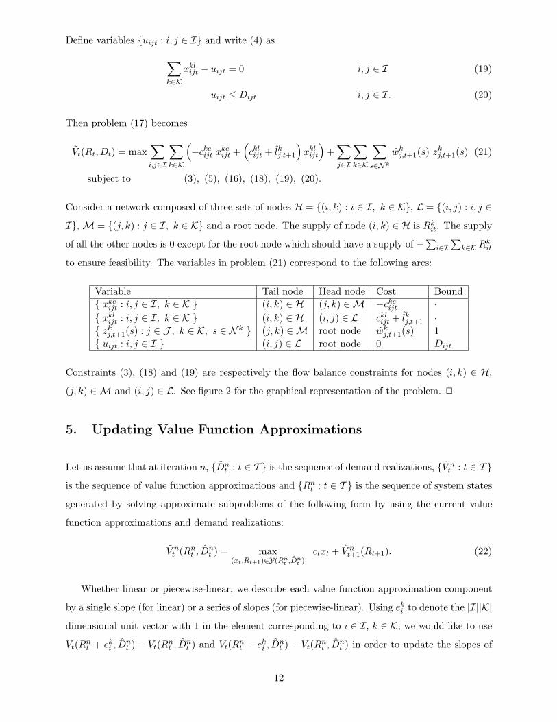
Define variables {uijt : i, j ∈ I} and write (4) as

∑

k∈Kxkl

ijt − uijt = 0 i, j ∈ I (19)

uijt ≤ Dijt i, j ∈ I. (20)

Then problem (17) becomes

Vt(Rt, Dt) = max∑

i,j∈I

∑

k∈K

(−cke

ijt xkeijt +

(cklijt + lkj,t+1

)xkl

ijt

)+

∑

j∈I

∑

k∈K

∑

s∈N k

wkj,t+1(s) zk

j,t+1(s) (21)

subject to (3), (5), (16), (18), (19), (20).

Consider a network composed of three sets of nodes H = {(i, k) : i ∈ I, k ∈ K}, L = {(i, j) : i, j ∈I}, M = {(j, k) : j ∈ I, k ∈ K} and a root node. The supply of node (i, k) ∈ H is Rk

it. The supply

of all the other nodes is 0 except for the root node which should have a supply of −∑i∈I

∑k∈KRk

it

to ensure feasibility. The variables in problem (21) correspond to the following arcs:

Variable Tail node Head node Cost Bound{ xke

ijt : i, j ∈ I, k ∈ K } (i, k) ∈ H (j, k) ∈M −ckeijt ·

{ xklijt : i, j ∈ I, k ∈ K } (i, k) ∈ H (i, j) ∈ L ckl

ijt + lkj,t+1 ·{ zk

j,t+1(s) : j ∈ J , k ∈ K, s ∈ N k } (j, k) ∈M root node wkj,t+1(s) 1

{ uijt : i, j ∈ I } (i, j) ∈ L root node 0 Dijt

Constraints (3), (18) and (19) are respectively the flow balance constraints for nodes (i, k) ∈ H,

(j, k) ∈M and (i, j) ∈ L. See figure 2 for the graphical representation of the problem. 2

5. Updating Value Function Approximations

Let us assume that at iteration n, {Dnt : t ∈ T } is the sequence of demand realizations, {V n

t : t ∈ T }is the sequence of value function approximations and {Rn

t : t ∈ T } is the sequence of system states

generated by solving approximate subproblems of the following form by using the current value

function approximations and demand realizations:

V nt (Rn

t , Dnt ) = max

(xt,Rt+1)∈Y(Rnt ,Dn

t )ctxt + V n

t+1(Rt+1). (22)

Whether linear or piecewise-linear, we describe each value function approximation component

by a single slope (for linear) or a series of slopes (for piecewise-linear). Using eki to denote the |I||K|

dimensional unit vector with 1 in the element corresponding to i ∈ I, k ∈ K, we would like to use

Vt(Rnt + ek

i , Dnt ) − Vt(Rn

t , Dnt ) and Vt(Rn

t − eki , D

nt ) − Vt(Rn

t , Dnt ) in order to update the slopes of

12

HHHHMMMMLLLL

( a , g )

( a , h )

( b , g )

( b , h )

( a , g )

( a , h )

( b , g )

( b , h )

( a , g )

( a , h )

( b , g )

( b , h )

( a , g )

( a , h )

( b , g )

( b , h )

( a , a )

( a , b )

( b , a )

( b , b ) ) ,0(

)1 ),(ˆ( )(

),ˆ(

),(

1,1,

1,

ijtijt

ktj

ltj

ktj

klijt

klijt

keijt

keijt

Du

swsz

lcx

cx

++

+ ∞+

∞−

Figure 2: Network representation of problem (21). We assume that I = {a, b}, K = {g, h}. Nodelabel (i, k) ∈ I ×K denotes that node (i, k) ∈ H or (i, k) ∈M. Node label (i, j) ∈ I2 denotes thatnode (i, j) ∈ L.

the value function approximation component V knit . However, this requires knowledge of the exact

value function. Instead, we propose using

Φnt (∓ek

i ) = V nt (Rn

t ∓ eki , D

nt )− V n

t (Rnt , Dn

t ). (23)

Here, we see another advantage of having min-cost network flow subproblems. For subproblems

with min-cost integer multicommodity flow structure, computing {Φnt (∓ek

i ) : i ∈ I, k ∈ K} requires

solving 2|I||K|+1 subproblems of form (22). However, if the subproblems are min-cost network flow

problems, then {Φnt (∓ek

i ) : i ∈ I, k ∈ K} can be computed by using flow augmenting-decreasing

paths, and this amounts to executing a shortest path algorithm only twice (Powell 1989).

5.1. Updating Linear Value Function Approximations

We assume that each linear value function approximation component V knit is characterized by the

slope vknit . Then, we set

vk,n+1it = (1− αn) vkn

it + αn Φnt (ek

i ), (24)

to obtain the slope of the value function approximation component V k,n+1it , where αn ∈ (0, 1) is

the step size at iteration n. We favor using Φnt (ek

i ) over Φnt (−ek

i ) merely because Φnt (−ek

i ) is not

13

defined when Rknit = 0.

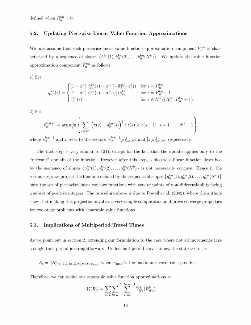
5.2. Updating Piecewise-Linear Value Function Approximations

We now assume that each piecewise-linear value function approximation component V knit is char-

acterized by a sequence of slopes{vknit (1), vkn

it (2), . . . , vknit (Nk)

}. We update the value function

approximation component V knit as follows:

1) Set

qknit (s) =

(1− αn) vknit (s) + αn (−Φn

t (−eki )) for s = Rkn

it

(1− αn) vknit (s) + αn Φn

t (eki ) for s = Rkn

it + 1vknit (s) for s ∈ N k\{Rkn

it , Rknit + 1}.

2) Set

vk,n+1it = arg min

z

∑

s∈Nk

(z(s)− qkn

it (s))2

: z(s) ≥ z(s + 1) s = 1, . . . , Nk − 1

,

where vk,n+1it and z refer to the vectors [vk,n+1

it (s)]s∈Nk and [z(s)]s∈N k respectively.

The first step is very similar to (24), except for the fact that the update applies only to the

“relevant” domain of the function. However after this step, a piecewise-linear function described

by the sequence of slopes{qknit (1), qkn

it (2), . . . , qknit (Nk)

}is not necessarily concave. Hence in the

second step, we project the function defined by the sequence of slopes{qknit (1), qkn

it (2), . . . , qknit (Nk)

}

onto the set of piecewise-linear concave functions with sets of points of non-differentiability being

a subset of positive integers. The procedure above is due to Powell et al. (2002), where the authors

show that making this projection involves a very simple computation and prove converge properties

for two-stage problems with separable value functions.

5.3. Implications of Multiperiod Travel Times

As we point out in section 2, extending our formulation to the case where not all movements take

a single time period is straightforward. Under multiperiod travel times, the state vector is

Rt = [Rkit′t]i∈I, k∈K, t≤t′<t+τmax , where τmax is the maximum travel time possible.

Therefore, we can define our separable value function approximations as

Vt(Rt) =∑

i∈I

∑

k∈K

t+τmax−1∑

t′=t

V kit′t(R

kit′t).

14

75

80

85

90

95

100

20 40 60 80 100%

of o

ptim

al o

bjec

tive

uppe

r bo

und

iteration number

single per. trav. tim.multiper. trav. tim. regular perf.multiper. trav. tim. accel. perf.

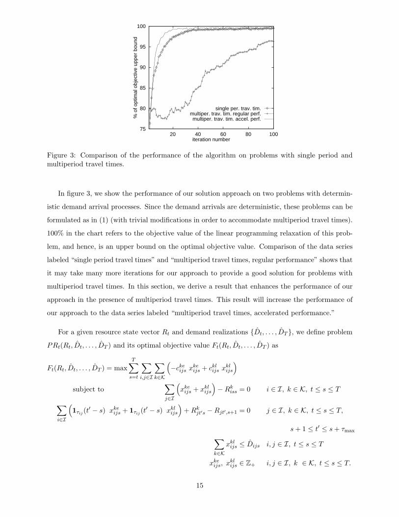
Figure 3: Comparison of the performance of the algorithm on problems with single period andmultiperiod travel times.

In figure 3, we show the performance of our solution approach on two problems with determin-

istic demand arrival processes. Since the demand arrivals are deterministic, these problems can be

formulated as in (1) (with trivial modifications in order to accommodate multiperiod travel times).

100% in the chart refers to the objective value of the linear programming relaxation of this prob-

lem, and hence, is an upper bound on the optimal objective value. Comparison of the data series

labeled “single period travel times” and “multiperiod travel times, regular performance” shows that

it may take many more iterations for our approach to provide a good solution for problems with

multiperiod travel times. In this section, we derive a result that enhances the performance of our

approach in the presence of multiperiod travel times. This result will increase the performance of

our approach to the data series labeled “multiperiod travel times, accelerated performance.”

For a given resource state vector Rt and demand realizations {Dt, . . . , DT }, we define problem

PRt(Rt, Dt, . . . , DT ) and its optimal objective value Ft(Rt, Dt, . . . , DT ) as

Ft(Rt, Dt, . . . , DT ) = maxT∑

s=t

∑

i,j∈I

∑

k∈K

(−cke

ijs xkeijs + ckl

ijs xklijs

)

subject to∑

j∈I

(xke

ijs + xklijs

)−Rk

iss = 0 i ∈ I, k ∈ K, t ≤ s ≤ T

∑

i∈I

(1τij (t

′ − s) xkeijs + 1τij (t

′ − s) xklijs

)+ Rk

jt′s −Rjt′,s+1 = 0 j ∈ I, k ∈ K, t ≤ s ≤ T,

s + 1 ≤ t′ ≤ s + τmax

∑

k∈Kxkl

ijs ≤ Dijs i, j ∈ I, t ≤ s ≤ T

xkeijs, xkl

ijs ∈ Z+ i, j ∈ I, k ∈ K, t ≤ s ≤ T.

15

The problem above can be viewed as the posterior multistage problem corresponding to demand

realization {Dt, . . . , DT }. Let {R∗t : t ∈ T } and {x∗t : t ∈ T } be the optimal solution to

PR1(R1, D1, . . . , DT ).

For the remainder of this section we denote the vector obtained by increasing the element

corresponding to i ∈ I, k ∈ K and t′ of R∗t by 1 as R∗

t + ekit′ . Therefore ek

it′ can be visualized as

a |I||K|τmax dimensional unit vector. However, the exact place of 1 becomes clear when it is used

together with R∗t . We have the following result.

Proposition 2 For all i ∈ I, k ∈ K, 1 ≤ t ≤ T − 1, t < t′ < t + τmax, we have

Ft

(R∗

t ∓ ekit′ , Dt, . . . , DT

)− Ft

(R∗

t , Dt, . . . , DT

)

≥ Ft+1

(R∗

t+1 ∓ ekit′ , Dt+1, . . . , DT

)− Ft+1

(R∗

t+1, Dt+1, . . . , DT

).

Proof We only show the case when the coefficient of ekit′ is positive.

We need to make three observations: 1) Since {R∗t : t ∈ T } and {x∗t : t ∈ T } are the optimal

solution to PR1(R1, D1, . . . , DT ), we have

Ft

(R∗

t , Dt, . . . , DT

)= ctx

∗t + Ft+1

(R∗

t+1, Dt+1, . . . , DT

). (25)

2) From the first observation, x∗t is a part of a feasible (and optimal) solution to PRt(R∗t , Dt, . . . , DT ).

Therefore x∗t is a part of a feasible (but not necessarily optimal) solution to PRt(R∗t +ek

it′ , Dt, . . . , DT ).

3) Applying decisions x∗t on R∗t generates the state vector R∗

t+1. Thus, applying decisions x∗t on

R∗t + ek

it′ generates the state vector R∗t+1 + ek

it′ . By observations 2 and 3, we have

Ft

(R∗

t + ekit′ , Dt, . . . , DT

)≥ ctx

∗t + Ft+1

(R∗

t+1 + ekit′ , Dt+1, . . . , DT

).

The result is obtained by subtracting (25) from the inequality above. 2

By repeated applications of proposition 2, we get

Ft

(R∗

t + ekit′ , Dt, . . . , DT

)− Ft

(R∗

t , Dt, . . . , DT

)(26)

≥ Ft+1

(R∗

t+1 + ekit′ , Dt+1, . . . , DT

)− Ft+1

(R∗

t+1, Dt+1, . . . , DT

)

≥ . . . ≥ Ft′−1

(R∗

t′−1 + ekit′ , Dt′−1, . . . , DT

)− Ft′−1

(R∗

t′−1, Dt′−1, . . . , DT

)

≥ Ft′(R∗

t′ + ekit′ , Dt′ , . . . , DT

)− Ft′

(R∗

t′ , Dt′ , . . . , DT

).

In effect, (26) states that the marginal value of a vehicle of type k ∈ K inbound to location

i ∈ I and time period t′ decreases over time. A similar chain of inequalities can be written for

Ft

(R∗

t − ekit′ , Dt, . . . , DT

)− Ft

(R∗

t , Dt, . . . , DT

), which proves the following result.

16

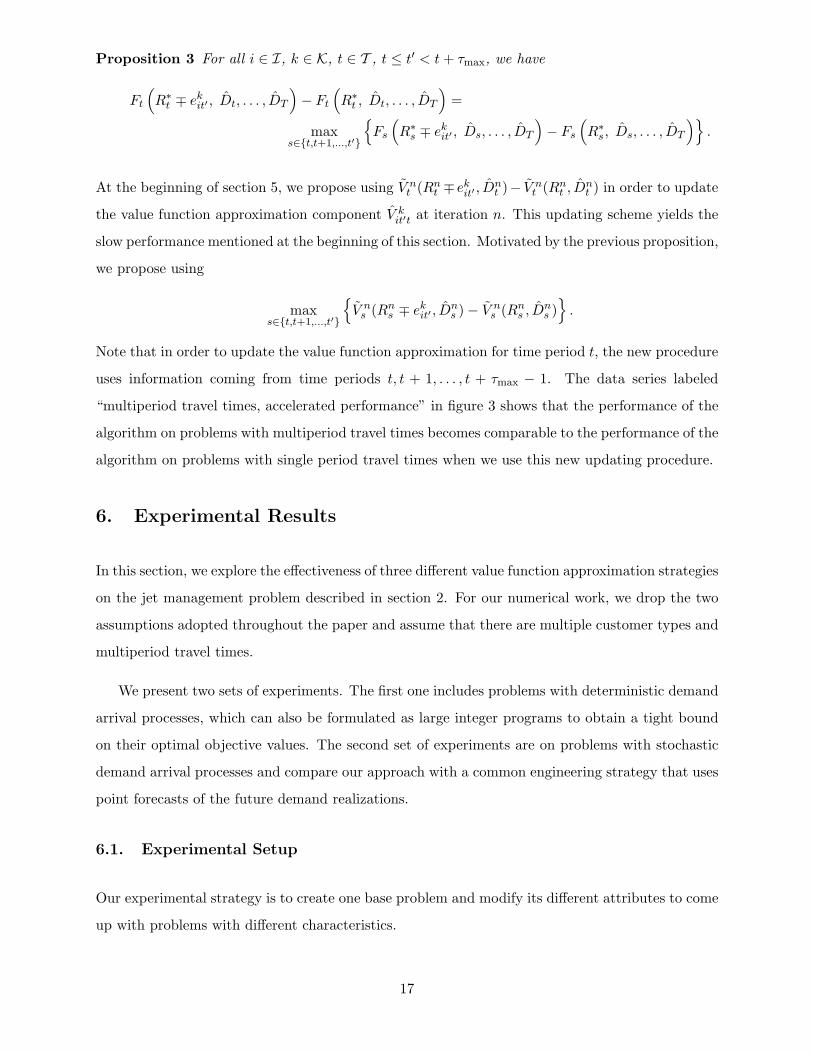
Proposition 3 For all i ∈ I, k ∈ K, t ∈ T , t ≤ t′ < t + τmax, we have

Ft

(R∗

t ∓ ekit′ , Dt, . . . , DT

)− Ft

(R∗

t , Dt, . . . , DT

)=

maxs∈{t,t+1,...,t′}

{Fs

(R∗

s ∓ ekit′ , Ds, . . . , DT

)− Fs

(R∗

s, Ds, . . . , DT

)}.

At the beginning of section 5, we propose using V nt (Rn

t ∓ ekit′ , D

nt )− V n

t (Rnt , Dn

t ) in order to update

the value function approximation component V kit′t at iteration n. This updating scheme yields the

slow performance mentioned at the beginning of this section. Motivated by the previous proposition,

we propose using

maxs∈{t,t+1,...,t′}

{V n

s (Rns ∓ ek

it′ , Dns )− V n

s (Rns , Dn

s )}

.

Note that in order to update the value function approximation for time period t, the new procedure

uses information coming from time periods t, t + 1, . . . , t + τmax − 1. The data series labeled

“multiperiod travel times, accelerated performance” in figure 3 shows that the performance of the

algorithm on problems with multiperiod travel times becomes comparable to the performance of the

algorithm on problems with single period travel times when we use this new updating procedure.

6. Experimental Results

In this section, we explore the effectiveness of three different value function approximation strategies

on the jet management problem described in section 2. For our numerical work, we drop the two

assumptions adopted throughout the paper and assume that there are multiple customer types and

multiperiod travel times.

We present two sets of experiments. The first one includes problems with deterministic demand

arrival processes, which can also be formulated as large integer programs to obtain a tight bound

on their optimal objective values. The second set of experiments are on problems with stochastic

demand arrival processes and compare our approach with a common engineering strategy that uses

point forecasts of the future demand realizations.

6.1. Experimental Setup

Our experimental strategy is to create one base problem and modify its different attributes to come

up with problems with different characteristics.

17

Problem T |I| |K| |D| R D c r C

Base 60 20 5 5 200 4000 4 5 I

T 30 30 20 5 5 200 2000 4 5 IT 90 90 20 5 5 200 6000 4 5 I

I 10 60 10 5 5 200 4000 4 5 II 40 60 40 5 5 200 4000 4 5 I

C II 60 20 5 5 200 4000 4 5 IIC III 60 20 5 5 200 4000 4 5 IIIC IV 60 20 5 5 200 4000 4 5 IV

R 1 60 20 5 5 1 4000 4 5 IR 5 60 20 5 5 5 4000 4 5 I

R 400 60 20 5 5 400 4000 4 5 IR 800 60 20 5 5 200 4000 4 5 I

c 1.6 60 20 5 5 200 4000 1.6 5 Ic 8 60 20 5 5 200 4000 8 5 I

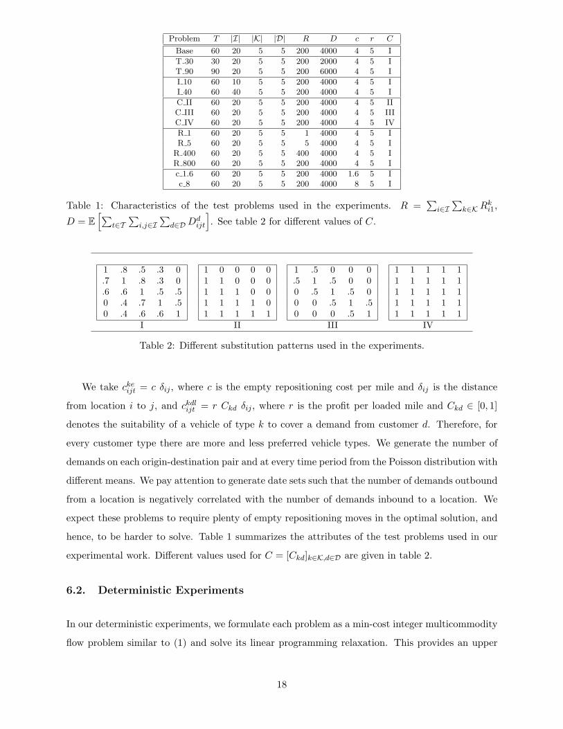
Table 1: Characteristics of the test problems used in the experiments. R =∑

i∈I∑

k∈KRki1,

D = E[∑

t∈T∑

i,j∈I∑

d∈D Ddijt

]. See table 2 for different values of C.

1 .8 .5 .3 0.7 1 .8 .3 0.6 .6 1 .5 .50 .4 .7 1 .50 .4 .6 .6 1

I

1 0 0 0 01 1 0 0 01 1 1 0 01 1 1 1 01 1 1 1 1

II

1 .5 0 0 0.5 1 .5 0 00 .5 1 .5 00 0 .5 1 .50 0 0 .5 1

III

1 1 1 1 11 1 1 1 11 1 1 1 11 1 1 1 11 1 1 1 1

IV

Table 2: Different substitution patterns used in the experiments.

We take ckeijt = c δij , where c is the empty repositioning cost per mile and δij is the distance

from location i to j, and ckdlijt = r Ckd δij , where r is the profit per loaded mile and Ckd ∈ [0, 1]

denotes the suitability of a vehicle of type k to cover a demand from customer d. Therefore, for

every customer type there are more and less preferred vehicle types. We generate the number of

demands on each origin-destination pair and at every time period from the Poisson distribution with

different means. We pay attention to generate date sets such that the number of demands outbound

from a location is negatively correlated with the number of demands inbound to a location. We

expect these problems to require plenty of empty repositioning moves in the optimal solution, and

hence, to be harder to solve. Table 1 summarizes the attributes of the test problems used in our

experimental work. Different values used for C = [Ckd]k∈K,d∈D are given in table 2.

6.2. Deterministic Experiments

In our deterministic experiments, we formulate each problem as a min-cost integer multicommodity

flow problem similar to (1) and solve its linear programming relaxation. This provides an upper

18

No. of iterations to reach Time (secs.)Max. obj. value Mean obj. value L P PL per iteration

Prob. L P PL L P PL 90 95 97.5 90 95 97.5 90 95 97.5 L P PL

Base 90.4 98.3 99.5 89.9 98.1 99.3 52 4 8 13 6 13 22 8 49 13

T 30 91.7 98.4 99.7 89.2 98.3 99.3 40 3 12 17 5 11 22 5 26 6T 90 90.5 98.6 99.3 88.3 98.5 99.0 44 3 7 14 5 11 16 13 71 19

I 10 93.8 99.7 99.8 92.3 99.5 99.7 15 2 4 8 4 5 11 2 12 6I 40 86.6 99.0 99.0 85.2 98.7 98.9 7 10 19 9 16 34 22 141 40

C II 91.3 99.4 98.8 90.1 99.2 98.5 41 2 6 12 5 11 22 7 82 15C III 88.5 98.7 99.7 87.2 98.6 99.7 3 13 19 5 13 24 6 39 9C IV 89.3 99.7 98.9 84.9 99.7 98.7 4 7 12 4 14 26 7 75 18

R 1 99.4 98.3 99.3 96.1 94.9 96.2 3 4 4 7 11 23 3 4 4 5 22 8R 5 97.1 97.4 95.0 95.2 94.2 93.3 10 32 3 9 42 61 6 48 9

R 100 91.6 97.7 97.2 90.1 97.6 97.0 50 14 16 10 44 7 47 9R 400 91.6 99.3 99.5 88.5 99.1 99.5 52 4 6 14 4 8 20 8 49 14

c 1.6 88.1 99.6 99.9 85.9 99.3 99.9 2 3 17 3 3 9 8 47 12c 8 92.9 98.3 98.6 91.1 98.2 98.5 45 8 14 24 10 21 39 8 45 12

Table 3: Results of deterministic runs.

bound on the optimal value of the objective function. We run the three different value function

approximation strategies described in section 4 for 150 iterations using the step size αn = 20/(40+n)

at iteration n. We concentrate on the objective function value of the last 50 iterations to eliminate

the effect of the “warming up” period of the value function approximations.

The results are shown in table 3. L, P and PL refer to linear, piecewise-linear and hybrid

value function approximation strategies described in sections 4.1, 4.2 and 4.3 respectively. In the

table, we give the average and maximum objective value in the last 50 iterations, and the number

of iterations required to reach a certain percentage of the upper bound on the optimal objective

value. The objective values we present are normalized to 100 by using the objective value of the

linear programming relaxation. The following observations can be made:

1) P and PL yield results within 1-2% of the upper bound. Considering its CPU time advantage,

PL seems to be an excellent approach for deterministic problems.

2) PL takes more iterations to reach a given solution quality, but it makes up for this difference

by faster runtime per iteration. Despite the fact that both L and PL solve min-cost network flow

subproblems, PL takes considerably more time per iteration due to the additional computational

burden brought by updating the piecewise-linear approximations and setting up the subproblems.

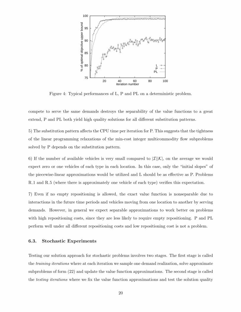
3) Figure 4 shows the typical performance of the three approximations. The objective value provided

by L fluctuates from one iteration to the next, whereas P and PL yield more stable behavior.

4) Although the presence of multiple types of vehicles that can exist in the same location and

19

75

80

85

90

95

100

20 40 60 80 100%

of o

ptim

al o

bjec

tive

uppe

r bo

und

iteration number

LP

PL

Figure 4: Typical performances of L, P and PL on a deterministic problem.

compete to serve the same demands destroys the separability of the value functions to a great

extend, P and PL both yield high quality solutions for all different substitution patterns.

5) The substitution pattern affects the CPU time per iteration for P. This suggests that the tightness

of the linear programming relaxations of the min-cost integer multicommodity flow subproblems

solved by P depends on the substitution pattern.

6) If the number of available vehicles is very small compared to |I||K|, on the average we would

expect zero or one vehicles of each type in each location. In this case, only the “initial slopes” of

the piecewise-linear approximations would be utilized and L should be as effective as P. Problems

R 1 and R 5 (where there is approximately one vehicle of each type) verifies this expectation.

7) Even if no empty repositioning is allowed, the exact value function is nonseparable due to

interactions in the future time periods and vehicles moving from one location to another by serving

demands. However, in general we expect separable approximations to work better on problems

with high repositioning costs, since they are less likely to require empty repositioning. P and PL

perform well under all different repositioning costs and low repositioning cost is not a problem.

6.3. Stochastic Experiments

Testing our solution approach for stochastic problems involves two stages. The first stage is called

the training iterations where at each iteration we sample one demand realization, solve approximate

subproblems of form (22) and update the value function approximations. The second stage is called

the testing iterations where we fix the value function approximations and test the solution quality

20

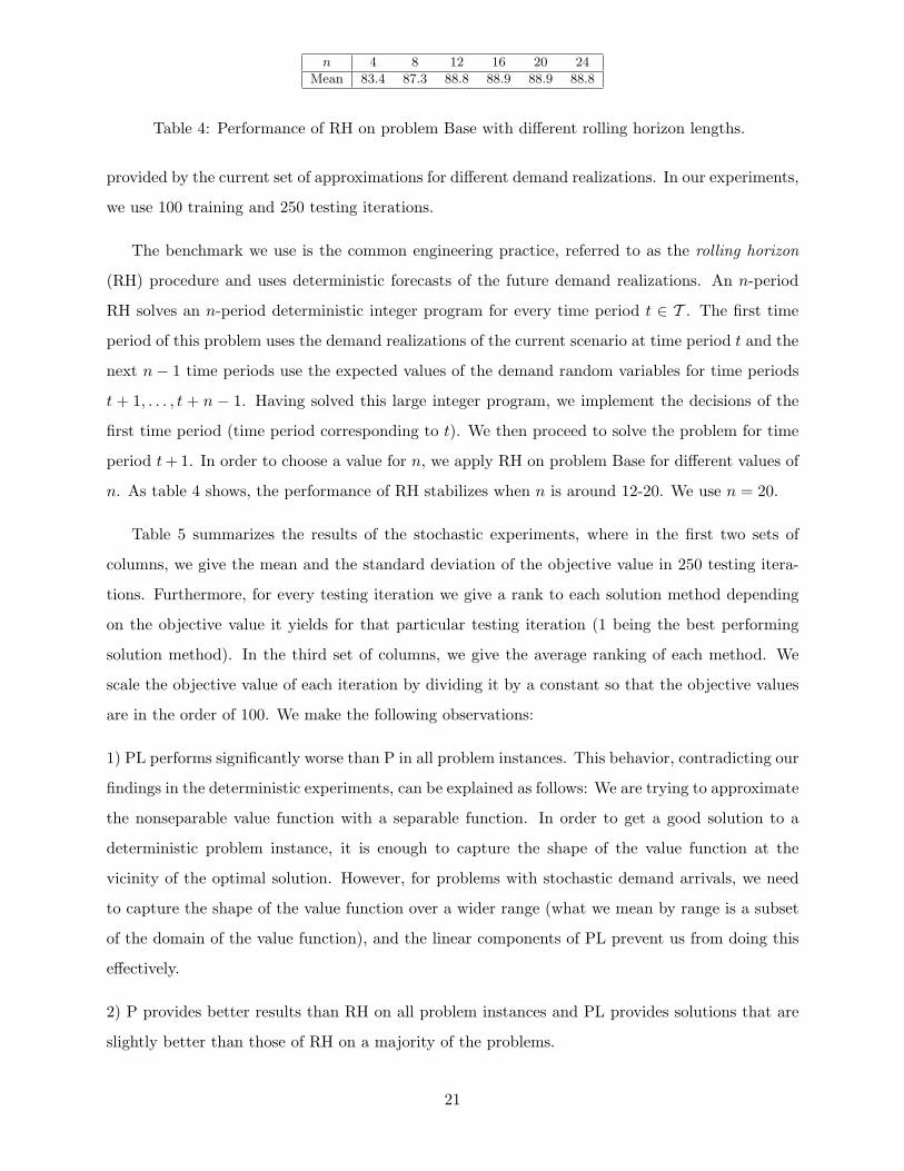
n 4 8 12 16 20 24

Mean 83.4 87.3 88.8 88.9 88.9 88.8

Table 4: Performance of RH on problem Base with different rolling horizon lengths.

provided by the current set of approximations for different demand realizations. In our experiments,

we use 100 training and 250 testing iterations.

The benchmark we use is the common engineering practice, referred to as the rolling horizon

(RH) procedure and uses deterministic forecasts of the future demand realizations. An n-period

RH solves an n-period deterministic integer program for every time period t ∈ T . The first time

period of this problem uses the demand realizations of the current scenario at time period t and the

next n− 1 time periods use the expected values of the demand random variables for time periods

t + 1, . . . , t + n − 1. Having solved this large integer program, we implement the decisions of the

first time period (time period corresponding to t). We then proceed to solve the problem for time

period t + 1. In order to choose a value for n, we apply RH on problem Base for different values of

n. As table 4 shows, the performance of RH stabilizes when n is around 12-20. We use n = 20.

Table 5 summarizes the results of the stochastic experiments, where in the first two sets of

columns, we give the mean and the standard deviation of the objective value in 250 testing itera-

tions. Furthermore, for every testing iteration we give a rank to each solution method depending

on the objective value it yields for that particular testing iteration (1 being the best performing

solution method). In the third set of columns, we give the average ranking of each method. We

scale the objective value of each iteration by dividing it by a constant so that the objective values

are in the order of 100. We make the following observations:

1) PL performs significantly worse than P in all problem instances. This behavior, contradicting our

findings in the deterministic experiments, can be explained as follows: We are trying to approximate

the nonseparable value function with a separable function. In order to get a good solution to a

deterministic problem instance, it is enough to capture the shape of the value function at the

vicinity of the optimal solution. However, for problems with stochastic demand arrivals, we need

to capture the shape of the value function over a wider range (what we mean by range is a subset

of the domain of the value function), and the linear components of PL prevent us from doing this

effectively.

2) P provides better results than RH on all problem instances and PL provides solutions that are

slightly better than those of RH on a majority of the problems.

21

Mean obj. value Std. dev. Mean rankProblem L P PL RH L P PL RH L P PL RH

Base 80.5 95.5 90.8 88.9 2.5 2.2 2.0 1.9 4.0 1.0 2.0 3.0

I 10 84.5 95.2 93.5 91.5 2.3 2.4 2.4 2.4 4.0 1.0 2.0 3.0I 40 74.1 92.2 87.3 86.9 1.8 0.5 0.6 0.8 4.0 1.0 2.0 3.0

C II 80.6 95.4 89.9 90.8 2.1 2.1 2.1 2.0 4.0 1.0 2.9 2.1C III 77.7 95.6 89.5 86.3 2.1 2.2 2.1 1.9 4.0 1.0 2.0 3.0C IV 82.8 95.5 92.4 92.2 2.6 2.2 2.1 2.2 4.0 1.0 2.3 2.7

R 1 88.9 85.2 73.2 52.9 7.6 8.7 9.0 8.4 1.0 2.0 3.0 4.0R 5 91.8 86.6 65.8 54.3 5.0 5.2 5.7 6.0 1.0 2.0 3.0 4.0

R 100 83.7 95.8 82.4 86.7 2.1 2.1 1.9 2.0 3.1 1.0 3.9 2.0R 400 83.0 95.0 93.9 90.2 2.2 2.2 2.1 2.0 4.0 1.0 2.0 3.0

c 1.6 73.8 95.6 94.4 90.6 2.1 2.1 2.0 1.9 4.0 1.0 2.0 3.0c 8 84.7 94.9 92.7 88.7 2.7 2.3 2.3 2.2 4.0 1.0 2.0 3.0

Table 5: Results of stochastic runs.

3) The CPU times for different approximation strategies are comparable to those for deterministic

experiments. The only computational burden brought by stochastic load arrival processes is the

need to draw a new sample realization at the beginning of each iteration.

4) In general, linear approximations yield poor solution quality. However, their fast runtimes may

make them attractive in the early iterations to initialize the piecewise-linear approximations, and

then we can switch to piecewise-linear or hybrid approximation strategies.

References

Aneja, Y. P., K. P. Nair. 1982. Multicommodity network flows with probabilistic loses. ManagementScience 28(9) 1080–1086.

Assad, A. A. 1978. Multicommodity network flows - A survey. Networks 8 37–91.

Bellman, R. 1957. Dynamic Programming. Princeton University Press, Princeton, NJ.

Bertsekas, D., J. Tsitsiklis. 1996. Neuro-Dynamic Programming. Athena Scientific, Belmont, MA.

Chen, Z. -L., W. B. Powell. 1999. A convergent cutting-plane and partial-sampling algorithm formultistage linear programs with recourse. Journal of Optimization Theory and Applications103(3) 497–524.

Chih, K. -K. 1986. A Real Time Dynamic Optimal Freight Car Management Simulation Model ofthe Multiple Railroad, Multicommodity Temporal Spatial Network Flow Problem. PhD thesis,Princeton University.

Crainic, T. G., M. Gendreau, P. Dejax. 1993. Dynamic and stochastic models for the allocation ofempty containers. Operations Research 41 102–126.

Godfrey, G. A., W. B. Powell. 2002. An adaptive, dynamic programming algorithm for stochasticresource allocation problems I: Single period travel times. Transportation Science 36(1) 21–39.

Hane, C., C. Barnhart, E. Johnson, R. Marsten, G. Nemhauser, G. Sigismondi. 1995. The fleet as-signment problem: Solving a large-scale integer program. Mathematical Programming 70 211–232.

Haneveld, W. K. K., M. H. van der Vlerk. 1999. Stochastic integer programming: General modelsand algorithms. Annals of Operations Research 85 39–57.

22

Higle, J., S. Sen. 1991. Stochastic decomposition: An algorithm for two stage linear programs withrecourse. Mathematics of Operations Research 16(3) 650–669.

Holmberg, K., M. Joborn, J. T. Lundgren. 1998. Improved empty freight car distribution. Trans-portation Science 32 163–173.

Jordan, W., M. Turnquist. 1983. A stochastic dynamic network model for railroad car distribution.Transportation Science 17 123–145.

Kennington, J. L. 1978. A survey of linear cost multicommodity network flows. Operations Research26 209–236.

Powell, W. B. 1989. A review of sensitivity results for linear networks and a new approximation toreduce the effects of degeneracy. Transportation Science 23(4) 231–243.

Powell, W. B., T. A. Carvalho. 1998. Dynamic control of logistics queueing network for large-scalefleet management. Transportation Science 32(2) 90–109.

Powell, W. B., P. Jaillet, A. Odoni. 1995. Stochastic and dynamic networks and routing. C. Monma,T. Magnanti and M. Ball, eds. Handbook in Operations Research and Management Science,Volume on Networks. North Holland, Amsterdam. 141–295.

Powell, W. B., A. Ruszczynski, H. Topaloglu. 2002. Learning algorithms for separable approxima-tions of stochastic optimization problems. Technical report, Princeton University, Princeton,NJ 08544.

Shan, Y. 1985. A Dynamic Multicommodity Network Flow Model For Real-Time Optimal RailFreight Car Management. PhD thesis, Princeton University.

Soroush, H. P., B. Mirchandani. 1990. The stochastic multicommodity flow problem. Networks20 121–155.

23