Dynamic Parameter Estimation and Optimization for Batch Distillation

Seyed Mostafa Safdarnejada, Jonathan R. Gallachera, John D. Hedengrena,∗

aDepartment of Chemical Engineering, 350 CB, Brigham Young University, Provo, UT 84602, USA

Abstract

This work reviews a well-known methodology for batch distillation modeling, estimation, and optimization

but adds a new case study with experimental validation. Use of nonlinear statistics and a sensitivity analysis

provides valuable insight for model validation and optimization verification for batch columns. The appli-

cation is a simple, batch column with a binary methanol-ethanol mixture. Dynamic parameter estimation

with an `1-norm error, nonlinear confidence intervals, ranking of observable parameters, and efficient sensi-

tivity analysis are used to refine the model and find the best parameter estimates for dynamic optimization

implementation. The statistical and sensitivity analyses indicated there are only a subset of parameters that

are observable. For the batch column, the optimized production rate increases by 14% while maintaining

product purity requirements.

Keywords: Dynamic Parameter Estimation, Nonlinear Statistics, Experimental Validation, Batch

Distillation, Dynamic Optimization

1. Introduction1

There are approximately 40,000 distillation columns in the US that are used to separate chemical com-2

pounds based on vapor pressure differences in industries ranging from oil and gas to pharmaceuticals. These3

separation columns consume 6% of the yearly US energy demand [1]. While many of the large production4

facilities use continuous processes, specialty and smaller-use items are often processed in batch columns5

[2, 3, 4]. Continuous distillation columns have been the focus of optimization work since the first column6

was built, but the transient nature of batch columns has caused many to remain unoptimized. The transient7

nature of the market for these specialty items has further hindered the optimization of batch columns [3].8

As a result, little research on batch column optimization is available in the literature before 1980 [5, 6, 7, 8].9

Work on batch columns has increased in the last 30 years as computers have become more sophisticated,10

and several studies have considered both advanced solving techniques and advanced column configurations11

[9, 10, 11, 12, 13, 14, 15, 16, 17, 18, 19, 20, 21, 22, 23]. Terwiesch, et al. [24] and Kim and Diwekar [25] provide12

a detailed history of the subject and a description of current batch distillation modeling and optimization13

methods.14

∗Corresponding author. Tel.: +1 801 477 7341, Fax: +1 801 422 0151Email addresses: safdarnejad@byu.edu (Seyed Mostafa Safdarnejad), jgallac2@byu.edu (Jonathan R. Gallacher),

john.hedengren@byu.edu (John D. Hedengren)

Preprint submitted to Computers & Chemical Engineering December 1, 2015

The optimization of the batch columns can be subdivided into optimal design problems and optimal15

control problems. Optimal design problems generally deal with column configuration, while optimal control16

problems deal with column operation. These ideas are summarized well in separations textbooks such as17

Diwekar [10], Stichlmair and Fair [26] and Doherty and Malone [27] and will therefore not be discussed18

further here. Research studies on this subject follow the same general outline as presented in the textbooks19

[3, 28]. The models developed for batch column optimization generally fall into two categories: first-principles20

models and shortcut or simple models.21

First-principles models are those with governing mass and energy balance equations, detailed thermo-22

dynamics, tray dynamics, system non-idealities and variable flow rates [29, 30, 31, 32]. These models are23

theoretically more accurate than shortcut methods, but they are only as accurate as the thermodynamic and24

physical property models they use [3]. The use of these models has been limited due to high computational25

costs. Several studies have been conducted using first-principles models and advanced solving techniques26

to reduce computational cost [33, 34, 35, 36, 37, 38, 39]. While these models accomplish the goal of re-27

ducing computational load, they are generally still slower than shortcut models. In addition, the lack of28

experimental data for batch columns makes it difficult to determine how much accuracy is lost when going29

from first-principles to lower-order (first-principles model with advanced or simplified numerical methods)30

to shortcut models [40].31

The second class of models, shortcut models, has received far greater attention. These models contain less32

physics and are generally used for ballpark estimates and comparative studies. A typical set of assumptions33

for these models is as follows: constant boil-up rate, no external heat loss, ideal stages, constant relative34

volatility, constant molar overflow, total condenser without subcooling and no column holdup [41, 42, 28,35

43, 31]. More recent shortcut models have kept most of the same assumptions while accounting for column36

dynamics using a non-zero column holdup [40, 36]. The primary purpose of these models is to create an37

accurate, computationally fast simulation for use in design and control of batch columns. While these models38

achieve the reduction in computational load, the lack of experimental data makes it difficult to determine39

the accuracy of these models [40]. The assumptions made in these models limit their use to ideal systems.40

The gap between first-principles models and shortcut models is large. First-principles models can provide41

predictions for many systems but require thermodynamic and physical property models as inputs, while the42

assumptions in shortcut models make them applicable only to a small class of relatively ideal systems. In this43

work, a method is proposed for developing shortcut models with relaxed assumptions. The method is based44

on fitting parameters in place of simplifying assumptions to include system non-idealities without solving the45

first-principles equations. Solving for the fitting parameters requires extensive experimental data whereas46

first-principles models typically need less data, being based on fundamental correlations. Dynamic parameter47

estimation can be used to reduce the experimental load. The case study presented in this work required only48

one experiment to determine model parameters. As with any model containing fitting parameters, there49

is concern over the accuracy of the parameters. By using nonlinear statistics [44] and a model sensitivity50

2

Select Parameters with

Sensi�vity Analysis

Parameter Es�ma�on for

Batch System with l 1-norm

Dead-Band Objec�ve

Nonlinear Confidence Region

for Batch System with

Bounds from F-sta�s�c

Dynamic Op�miza�on for

Batch System with l 1-norm

Dead-Band Trajectory

Objec�ve

Collect Dynamic Data Modify Equa�ons

Op�mized Produc�on

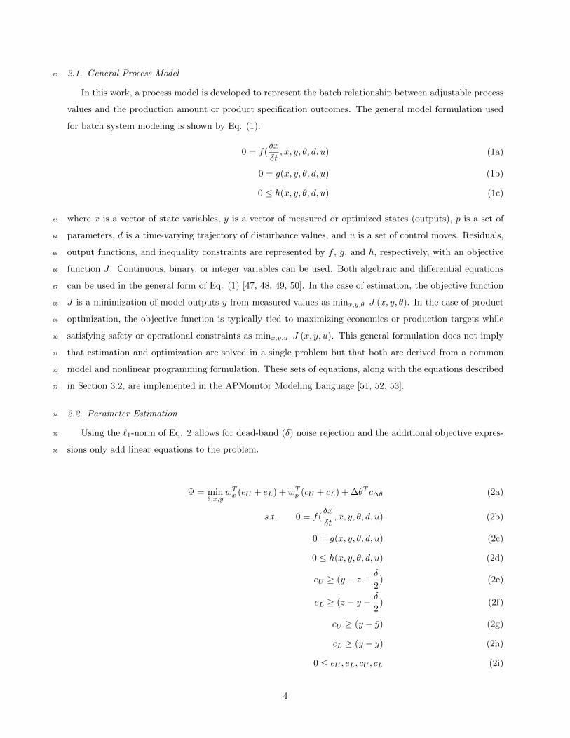
Figure 1: Overview of methodology for batch column optimization with novel contributions underlined

analysis [45], it is possible to determine how many parameters can be estimated from the collected data and51

the acceptable range for those parameters. These steps are shown in Figure 1 and form the heart of the52

method. Underlined elements of the methodology indicate the new approach to batch separation systems.53

The well-known methodology shown in Figure 1 is applied to an experimental case study. The method-54

ology includes the use of `1-norm dynamic parameter estimation, nonlinear statistics [44, 46], and a model55

parameter sensitivity analysis [45]. These techniques are applied together to a batch distillation column56

in a holistic approach to dynamic optimization. Models developed using this method account for system57

non-idealities not seen in typical shortcut models without sacrificing computational speed.58

2. Model Development Framework59

In this section, the general equations used to represent the process model, parameter estimation, nonlinear60

statistics and sensitivity analysis, or process optimization are reviewed.61

3

2.1. General Process Model62

In this work, a process model is developed to represent the batch relationship between adjustable process

values and the production amount or product specification outcomes. The general model formulation used

for batch system modeling is shown by Eq. (1).

0 = f(δx

δt, x, y, θ, d, u) (1a)

0 = g(x, y, θ, d, u) (1b)

0 ≤ h(x, y, θ, d, u) (1c)

where x is a vector of state variables, y is a vector of measured or optimized states (outputs), p is a set of63

parameters, d is a time-varying trajectory of disturbance values, and u is a set of control moves. Residuals,64

output functions, and inequality constraints are represented by f , g, and h, respectively, with an objective65

function J . Continuous, binary, or integer variables can be used. Both algebraic and differential equations66

can be used in the general form of Eq. (1) [47, 48, 49, 50]. In the case of estimation, the objective function67

J is a minimization of model outputs y from measured values as minx,y,θ J (x, y, θ). In the case of product68

optimization, the objective function is typically tied to maximizing economics or production targets while69

satisfying safety or operational constraints as minx,y,u J (x, y, u). This general formulation does not imply70

that estimation and optimization are solved in a single problem but that both are derived from a common71

model and nonlinear programming formulation. These sets of equations, along with the equations described72

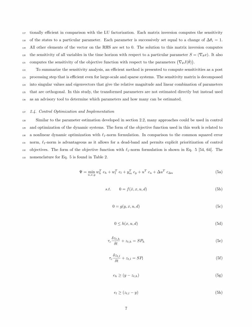
in Section 3.2, are implemented in the APMonitor Modeling Language [51, 52, 53].73

2.2. Parameter Estimation74

Using the `1-norm of Eq. 2 allows for dead-band (δ) noise rejection and the additional objective expres-75

sions only add linear equations to the problem.76

Ψ = minθ,x,y

wTx (eU + eL) + wTp (cU + cL) + ∆θT c∆θ (2a)

s.t. 0 = f(δx

δt, x, y, θ, d, u) (2b)

0 = g(x, y, θ, d, u) (2c)

0 ≤ h(x, y, θ, d, u) (2d)

eU ≥ (y − z +δ

2) (2e)

eL ≥ (z − y − δ

2) (2f)

cU ≥ (y − y) (2g)

cL ≥ (y − y) (2h)

0 ≤ eU , eL, cU , cL (2i)

4

Table 1: Nomenclature for general form of the objective function with `1-norm formulation for dynamic data reconciliation

Symbol Description

Ψ minimized objective function result

y model outputs (y0, . . . , yn)T

z measurements (z0, . . . , zn)T

y prior model outputs (y0, . . . , yn)T

wTx measurement deviation penalty

wTp penalty from the prior solution

c∆θ penalty from the prior parameter values

δ dead-band for noise rejection

x, u, θ, d states (x), inputs (u), parameters (θ), or unmeasured dis-

turbances (d)

∆θT change in parameters

f, g, h equations residuals (f), output function (g), and inequality

constraints (h)

eU , eL slack variable above and below the measurement dead-

band

cU , cL slack variable above and below a previous model value

The nomenclature for Eq. 2 is found in Table 1.77

Many approaches can be used to find the parameters, two of which are least squares formulation and78

`1-norm formulation for the objective function. The least squares objective is more sensitive to bad data such79

as outliers as shown later in Figure 5. The `1-norm method is less sensitive to outliers and the form of the80

objective function used in this `1-norm formulation is smooth and continuously differentiable as opposed to81

using the absolute value function. A more thorough comparison of the `1-norm and least squares is provided82

in [54].83

2.3. Confidence Intervals and Sensitivity Analysis84

Reliability of the parameters is investigated by implementing an approximate nonlinear confidence interval85

calculation [44]. Non-linear confidence intervals can be found by solving Eq. 3 for the sets of parameters86

that make up the joint confidence region [55], then extracting the upper and lower bounds of that region in87

each dimension.88

J(θ)− J(θ∗)

J(θ∗)≤ p

n− pFn,n−p,1−α (3)

In Eq. 3, J(θ) is the error between the measurements and the model prediction at a value θ of the89

parameters, J(θ∗) is the error between the measurements and the model prediction at the best estimates90

5

of the parameters (θ∗), p is the number of parameters in the model, n is the number of data points, and91

Fn,n−p,1−α is the F-statistic at n and n− p degrees of freedom with a confidence level of 1−α. The squared92

error objective is the only form of the nonlinear confidence interval that has a theoretical foundation. This93

is because the F-statistic used to define the confidence region is a ratio of χ2 distributions that compares the94

equivalence of two sets of experimental results. The χ2 distributions are intended for least square objectives95

instead of `1-norm objectives. According to the authors’ knowledge, an equivalent F-statistic for nonlinear96

confidence intervals and the `1-norm has not been derived. A nonlinear confidence interval for `1-norm97

objectives based on the F-statistic is future work.98

It is also desirable to determine the number of parameters that can be estimated or are observable given99

a particular model form and set of data. Large confidence intervals signal that a particular parameter may100

not be observable or that the effect of that parameter may be co-linearly dependent with other parameters.101

A well-known systematic analysis is used to determine which parameters can be estimated and rank the102

parameters in terms of the ability of a particular parameter to improve a particular model estimate [45, 56].103

This procedure is accomplished in 3 steps: (1) efficient computation of the sensitivities, (2) scaling of the104

dynamic parameter sensitivities, and (3) singular value decomposition of the scaled sensitivity matrix to105

reveal an optimal parameter space transformation.106

The first step in performing the parameter analysis is to compute the state dependencies to changes in107

the parameters. This can be accomplished with a variety of methods. One such method is to compute a finite108

difference sensitivity of the parameters with a series of perturbed simulations [57, 58]. A second method109

is to augment the model with adjoint equations that compute sensitivities simultaneously with the model110

predictions [59]. A third method is a post-processing method with time-discretized solutions to differential111

equation models [60, 61, 62]. This post-processing method involves efficient solutions to a linear system of112

equations, especially over other methods for large-scale and sparse systems [63].113

The sensitivity is computed from time-discretized models that are solved by nonlinear programming

solvers. At the solution, exact first derivatives of the equations with respect to variables are available

through automatic differentiation. These derivatives are available with respect to the states (∇fx(x, θ)) and

parameters (∇fp(x, θ)). For the objective function, objective gradients are computed with respect to states

(∇Jx(x, θ)) and parameters (∇Jθ(x, θ)). Sparsity in those matrices is exploited to improve computational

performance, especially for large-scale systems. Sensitivities are computed by solving a set of linear equations

as shown in Eq. 4 with parameter values fixed at θ and variable solution x as nominal values.∇xf(x, θ) ∇θf(x, θ) 0

∇xJ(x, θ) ∇θJ(x, θ) −1

0 I 0

∇θx

∇θθ

∇θJ(θ)

=

0

∆θi = 1

0

(4)

To further improve the efficiency of this implementation, an LU factorization of the left hand side (LHS)114

mass matrix is computed. This LU factorization is preserved for successive solutions of the different right115

hand side (RHS) vectors because the LHS does not change and successive sparse back-solves are computa-116

6

tionally efficient in comparison with the LU factorization. Each matrix inversion computes the sensitivity117

of the states to a particular parameter. Each parameter is successively set equal to a change of ∆θi = 1.118

All other elements of the vector on the RHS are set to 0. The solution to this matrix inversion computes119

the sensitivity of all variables in the time horizon with respect to a particular parameter S = (∇θx). It also120

computes the sensitivity of the objective function with respect to the parameters(∇θJ(θ)

).121

To summarize the sensitivity analysis, an efficient method is presented to compute sensitivities as a post122

processing step that is efficient even for large-scale and sparse systems. The sensitivity matrix is decomposed123

into singular values and eigenvectors that give the relative magnitude and linear combination of parameters124

that are orthogonal. In this study, the transformed parameters are not estimated directly but instead used125

as an advisory tool to determine which parameters and how many can be estimated.126

2.4. Control Optimization and Implementation127

Similar to the parameter estimation developed in section 2.2, many approaches could be used in control128

and optimization of the dynamic systems. The form of the objective function used in this work is related to129

a nonlinear dynamic optimization with `1-norm formulation. In comparison to the common squared error130

norm, `1-norm is advantageous as it allows for a dead-band and permits explicit prioritization of control131

objectives. The form of the objective function with `1-norm formulation is shown in Eq. 5 [54, 64]. The132

nomenclature for Eq. 5 is found in Table 2.133

Ψ = minu,x,y

wTh eh + wTl el + yTm cy + uT cu + ∆uT c∆u (5a)

s.t. 0 = f(x, x, u, d) (5b)

0 = g(y, x, u, d) (5c)

0 ≤ h(x, u, d) (5d)

τcδzt,hδt

+ zt,h = SPh (5e)

τcδzt,lδt

+ zt,l = SPl (5f)

eh ≥ (y − zt,h) (5g)

el ≥ (zt,l − y) (5h)

7

Table 2: Nomenclature for general form of the objective function with `1-norm formulation

Symbol Description

Ψ minimized objective function result

y model outputs (y0, . . . , yn)T

zt, zt,h, zt,l desired trajectory target or dead-band

wh, wl penalty factors outside trajectory dead-band

cy, cu, c∆u cost of variables y, u, and ∆u, respectively

u, x, d inputs (u), states(x), and parameters or disturbances(d)

f, g, h equation residuals(f), output function (g), and inequality

constraints (h)

τc time constant of desired controlled variable response

el, eh slack variable below or above the trajectory dead-band

SP, SPlo, SPhi target, lower, and upper bounds to final set point dead-

band

3. Dynamic Estimation and Optimization for a Batch Distillation Column134

This established methodology is demonstrated for the first time on a binary batch distillation column.135

While the methods are not new, the application to this specific column is novel and gives experimental136

insight on issues encountered when applying dynamic optimization on applications that share common137

features. This section is subdivided into a brief discussion of the apparatus and experimental procedure,138

parameter estimation and validation, and model optimization and validation.139

3.1. Apparatus and Experimental Procedure140

A 38 tray, 2 inch, vacuum-jacketed and silvered Oldershaw column is used to collect all experimental data141

(see Figure 2). Cooling water supplies the energy sink for the total condenser at the top of the column. A142

600 W reboiler heater is the only source of energy input. Reflux ratio is set using a swinging bucket and can143

be changed as frequently as every 5 minutes. The instantaneous distillate composition is determined using144

the refractive index of the solution and the total distillate collected is determined via a graduated cylinder.145

Cumulative distillate composition can be measured and inferred using the instantaneous compositions and146

a mass balance. The instantaneous distillate composition can be measured every 5 minutes. The reboiler147

is initially charged with 1.5 L of a 50/50 wt% mixture of methanol and ethanol for each run, with the goal148

being a product of 99 mol% methanol.149

The non-optimized base case experiment consists of running the column at total reflux for 30 minutes,150

then setting the reflux ratio to a constant value, usually somewhere between 3 and 5, and letting the column151

run until the cumulative overhead composition reaches 99 mol% methanol. The collection time usually lasts152

60 to 90 minutes, depending on the reflux ratio. The instantaneous and cumulative compositions for a typical153

8

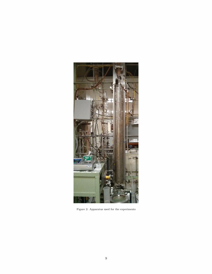
Figure 2: Apparatus used for the experiments

9

run, as well as the amount of product collected, can be seen in Figures (3a) and (3b), respectively. In this154

case, running the column at total reflux for 30 minutes, then using a constant reflux ratio of 4 for the next155

90 minutes resulted in 13.7 moles of 99 mol% methanol.156

0 20 40 60 80 100 120 140 1600.5

0.6

0.7

0.8

0.9

1

Co

mp

ositio

n (

mo

l fr

ac)

Time (min)

Base Cumulative

Base Instantaneous

Purity Spec

(a) Instantaneous and cumulative product mole fraction

0 20 40 60 80 100 120 140 1600

5

10

15

20

Pro

du

ctio

n (

mo

l)

Time (min)

Methanol Production

(b) Methanol production

Figure 3: Non-optimized base case where the final required purity (> 99 mol% ethanol) is not met

3.2. Equations for the Simplified Process Model157

Distillation is an inherently complex process involving mass and energy transfer, thermodynamics, and158

often reaction kinetics. Models that describe these phenomena do not have to be complex, however. The159

model developed here is used to describe the separation of a 50/50 wt% mixture of methanol and ethanol,160

and is simple by design to illustrate this point.161

The VLE model used here is found in the CHEMCAD database [65] and is shown in Eq. 6:

y∗n = −2.016x4n + 0.6861x3

n − 1.206x2n + 1.721xn + 0.0003984 (6)

where xn is the liquid mole fraction of methanol and y∗n is the vapor mole fraction of methanol in equilibrium

with the liquid. The subscript n denotes the stage for which the mole fraction is being calculated. An

adjustment to the equilibrium vapor mole fraction is used because equilibrium is not often achieved during

column operation. This adjustment is in the form of a Murphree efficiency and is shown in Eq. 7:

yn = yn+1 − EMV (yn+1 − y∗n) (7)

where yn is the actual mole fraction and EMV is the efficiency. The efficiency is a fitting parameter used to162

account for system non-idealities and is found using the data collected as part of this work.163

The liquid mole fraction for each stage is found by performing a material balance at each stage, n, as164

shown by Eq. 8 where V is the vapor flow through the column, L is the liquid return flow, and Ntray is the165

number of moles of liquid on the stage. The number of moles and the composition in the reboiler (Nreb and166

xreb) change with time and are represented by Eqs. 9 - 10. The number of moles in the condenser (Ncond)167

is assumed constant while the composition of the condenser (xcond) varies throughout the run (see Eq. 11).168

Variation of the number of moles and composition of the product with time are represented by Eqs. 12 and169

10

13. The liquid holdup for the condenser and trays are also design variables and are described in Eqs. 14 and170

15, where ftray and fcond are the fitting parameters representing the fraction of the initial reboiler charge171

on each tray and in the condenser, respectively. The tray holdup is assumed constant across all stages. The172

stages are numbered from 1 to 40 with the top being 1 (condenser).173

dxndt

=L(xn−1 − xn)− V (yn − yn+1)

Ntray(8)

xrebdNrebdt

+Nrebdxrebdt

= Lx39 − V yreb (9)

dNrebdt

= L− V (10)

Nconddxconddt

= V (y2 − xcond) (11)

dnpdt

= D (12)

xpdnpdt

+ npdxpdt

= D xcond (13)

Ncond = Nreb.init fcond (14)

Ntray = Nreb.init ftray (15)

The vapor flow rate is found using the energy balance shown in Eq. 16:

V =hdot hfHvap

(16)

where hdot is the heat input from the heater, Hvap is the heat of vaporization for the methanol/ethanol system,

and hf is a fitting parameter representing the heating efficiency. The heat of vaporization is approximated

as a weighted average of the pure component heats of vaporization obtained from the DIPPR Database [66].

The liquid flow rate, the reflux ratio, and the distillate rate are found using an overall mass balance and the

definition of the reflux ratio, shown in Eqs. 17 and 18, respectively:

V = L+D (17)

R =L

D(18)

where R is the reflux ratio and D is the distillate rate. Constant molar overflow is assumed throughout the174

model and applies to the equations shown above.175

11

3.3. Equations for the Detailed Process Model176

A more detailed (although not completely from first-principles) model [67] with energy balance equations177

validates the simplified model developed in Section 3.2. A similar notation as the simplified model is used178

for the detailed model with a distinction in the stage number in which the material and energy balances are179

developed. Vapor and liquid leaving each stage are noted as Vn and Ln, respectively. The equations used in180

the detailed model are based on the following assumptions:181

• constant molar hold up for the condenser and trays182

• fast heat transfer throughout the column183

• liquid temperature on each tray at the mixture bubble point184

• vapor liquid equilibrium relationships based on temperature dependent vapor pressures185

• pressure drop across each tray is 1 mmHg = ∆P186

• temperature dependent density, heat capacity, vapor pressure, and heat of vaporization187

The overall and component mole balances as well as the energy balance equation for a control volume188

over the condenser and accumulator lead to Eqs. 19 to 22.189

V2 = L1 +D (19)

L1 = R D (20)

Nconddxcond

dt= V2 y2 − (L1 +D) xcond (21)

Qcond = V2 hV2 − (L1 +D) hL1 (22)

A component and overall mole balance over the trays result in Eqs. 23 and 24. Eq. 25 also represents190

an energy balance for each tray in the column.191

Ntraydxndt

= Ln−1 xn−1 − Ln xn + Vn+1 yn+1 − Vn yn (23)

0 = Vn+1 − Vn + Ln−1 − Ln (24)

Vn+1 (hVn+1 − hLn) = Vn (hVn − hLn)− Ln−1 (hLn−1 − hLn) (25)

12

A component mole balance and the associated energy balance equation for the reboiler are presented by192

Eqs. 26 and Eq. 27. The reboiler heating rate, Qreb, is 600 W to drive the separation together with the193

cooling of the condenser, Qcond. The overall mole balance for this model is similar to the simplified model194

(Eq. 10).195

xrebdNrebdt

+Nrebdxrebdt

= L39 x39 − V40 yreb (26)

Qreb hf = V40 (hV40− hL40

)− L39 (hL39− hL40

) (27)

Accumulation of product and the change in composition of the product with respect to changes in product196

moles are shown in Eqs. 12 and 13. The enthalpy of mixture for both liquid and gas phases is a mole average197

of the enthalpy of each component. Enthalpy of each component is obtained by integrating the heat capacity198

for liquid and adding the heat of vaporization for vapor. The temperature profile in the column is also a199

function of the equilibrium composition of each stage. The relationship between temperature and liquid200

composition of each stage is based on vapor pressure and the pressure on each tray (Pn) as shown in 28 with201

ns = 2.202

P1 = 0.86 atm (Ambient Pressure in Provo, UT) (28a)

Pn = Pn−1 −∆P (28b)

Pn =

ns∑i=1

γi xi Psati (Ti) (28c)

The vapor composition at each tray is determined by the vapor liquid equilibrium correlation shown in203

Eq. 29 and is combined with the previous Eq. 7 to relate the equilibrium composition (y∗n) to the actual204

tray composition (yn) based on the Murphree efficiency.205

y∗n Pn = γ xn Psatn (Tn) (29)

A full listing of the model equations, data, and Python source code is given in Appendix A. The more206

sophisticated model demonstrates that the simpler and less rigorous model is able to adequately predict the207

batch column performance for the purpose of optimization. The model validation is shown in the subsequent208

section.209

3.4. Model Validation210

Model validation is accomplished through dynamic parameter estimation. The parameter estimation211

experiment was similar to a doublet test, with reflux ratios set to 3.5, 1, 7 and 3.5. The column was allowed212

to come to steady state at infinite reflux before starting data collection; the reflux ratio was adjusted every 15213

minutes thereafter. The parameters found by fitting the model with experimental data are heater efficiency214

13

time(min)

0 10 20 30 40 50 60

xA m

eth

an

ol

0.5

0.6

0.7

0.8

0.9

1

Simplified (l1-norm)

Simplified (sq. error)

Rigorous (l1-norm)

Rigorous (sq. error)

Measured Composition

(a) Instantaneous distillate composition

time(min)

0 10 20 30 40 50 60

pro

duct m

ole

s

0

5

10

15

Simplified (l1-norm)

Simplified (sq. error)

Rigorous (l1-norm)

Rigorous (sq. error)

Measured Methanol Moles

(b) Methanol production

Figure 4: Model validation for initial parameter estimation

(hf ), vaporization efficiency (EMV ), condenser molar holdup as a fraction of initial reboiler charge (fcond),215

and tray molar holdup as a fraction of initial reboiler charge (ftray). The parameter best estimates are216

shown in Table 3.217

Table 3: Confidence interval calculation for the four parameter case

Parameter Best Estimate Upper 95% CI Lower 95% CI

hf 0.719 0.799 0.639

EMV 0.691 2.420 0

fcond 0.029 0.254 0

ftray 5.077e-4 0.142 0

The instantaneous distillate composition from the experimental run and the associated simplified and218

detailed model predictions using optimized parameters are shown in Figure (4a). The maximum error219

between the simplified model predictions and the experimental values is 10%. The maximum error between220

the more detailed model and experimental composition data is 4.8% for the `1-norm objective and 5.3% for221

the squared error objective. Cumulative methanol production is shown in Figure (4b). The error between222

model and prediction is almost non-existent using both an `1-norm or squared error objective. The simplified223

model parameter estimation has 3,510 equations with the squared error objective and 3,780 equations with224

the `1-norm objective and requires less than 10 CPU seconds to solve. The more detailed model parameter225

estimation has 11,644 equations with the squared error objective and 11,972 equations with the `1-norm226

objective and requires 89.4 (`1-norm) and 53.1 (squared error) CPU seconds to solve. All calculations227

are performed on a Intel Core i7-2760QM CPU operating at 2.4 GHz with the APOPT solver. Because the228

simplified model produces similar results to the detailed model and solves sufficiently fast for online real-time229

optimization, it is selected for the batch column optimization.230

If artificial outliers are introduced in both the composition (80 mol% ethanol at t = 10 min and t =231

50 min) and cumulative production (15 moles at t = 30 min and t = 50 min), the squared error predictions232

deviate while the `1-norm estimates do not (see Figure 5).233

14

time(min)

0 10 20 30 40 50 600.6

0.65

0.7

0.75

0.8

0.85

0.9

0.95

1

1.05

Predicted Methanol Composition (l1-norm)

Predicted Methanol Composition (sq. error)

Measured Methanol Composition

(a) Instantaneous distillate composition

time(min)

0 10 20 30 40 50 600

5

10

15

Predicted Methanol Moles (l1-norm)

Predicted Methanol Moles (sq. error)

Measured Methanol Moles

(b) Methanol production

Figure 5: Insensitivity of the `1-norm estimation to outliers compared to the squared error objective

While this particular example did not include significant outliers, many industrial applications of batch234

distillation may have instruments that report values with drift, noise, or outliers [68]. While gross error235

detection can resolve many of these data quality issues, it is also desirable to have estimation methods that236

are less sensitive to bad data as shown in this example.237

3.5. Testing the Reliability of the Estimated Parameters238

Nonlinear confidence intervals are calculated for four potential parameters. Confidence regions are typ-239

ically reported as upper and lower limits on a particular parameter. This work extends the nonlinear con-240

fidence region to multivariate analysis that improve co-linearity assessment for batch distillation processes241

beyond a singular value decomposition or linear analysis. However, a look at the confidence interval for each242

individual parameter is useful to illustrate the procedure for model validation. A wide confidence interval243

suggests that there is insufficient structure in the model (observability) to determine the parameters from244

available measurements. Another insight that is gained from the confidence intervals is a test of the data245

diversity that leads to tight confidence regions. A tighter confidence region implies that a smaller deviation246

of the parameter from an optimal value is not statistically likely given a set of data to which the model247

is reconciled. Table 3 shows the expected value and 95% confidence interval for each parameter. As seen248

in the table, the interval for heater efficiency is narrow and in the range of values expected for a heater.249

The intervals for the other three parameters are large enough to include zero and the interval for vapor250

efficiency includes physically impossible values. Although the fit between model and data is excellent there251

are large parameter confidence intervals. One possible explanation for the large intervals is that the model is252

over-parameterized and thus has too many degrees of freedom. Thus, a sensitivity analysis is implemented253

to investigate the correct parameterization of the model.254

The scaled sensitivity is shown graphically in Figure 6. The sensitivity is scaled by solution values255

as Si,j =(∇θjxi

)θixi

to show relative effects with a unitless transformation. The scaling is applied with256

parameters θ and variables x at solution values.257

15

0 10 20 30 40 50 60−0.2

0

0.2

0.4

0.6

0.8

1

Pro

duction S

ens (

np)

Heater Efficiency (d(np)/d(h

f)

Vapor Efficiency (d(np)/d(E

MV))

Condenser Fraction (d(np)/d(cond

f))

Tray Fraction d(np)/d((tray

f))

0 10 20 30 40 50 60−0.3

−0.2

−0.1

0

0.1

0.2

Time (min)

Mole

Fra

c S

ens (

x 1)

Heater Efficiency (d(x1)/d(h

f)

Vapor Efficiency (d(x1)/d(E

MV))

Condenser Fraction (d(x1)/d(cond

f))

Tray Fraction d(x1)/d((tray

f))

Figure 6: Scaled variable sensitivities to the parameters

One clear result from this sensitivity study is that the total production (np) is dependent on the heat258

input to the batch column and that other parameters have little effect on the total production. As expected,259

a higher heating rate (hf ) vaporizes additional liquid and increases the flow to the condenser. With a260

specified reflux rate, the total production rate increases proportionally. In other words, a 1% increase in261

heating produces 1% additional product. This scaled sensitivity is shown as a value of 1.0 in the top subplot262

of Figure 6. The sensitivities of instantaneous product composition to the parameters are nearly co-linear as263

seen by the bottom subplot of Figure 6. For example, heater efficiency (hf ) and tray holdup fraction (ftray)264

can be increased and decreased, respectively, to produce nearly the same final answer. Other parameters265

also show a high degree of co-linearity.266

While sensitivity plots such as Figure 6 are instructive, it can be difficult for large-scale systems to detect267

co-linearity or the number and selection of parameters that can be estimated from the data. An alternative268

way to show the same information is to decompose the sensitivity matrix with a singular value decomposition269

to reveal magnitudes of singular values (relative importance of transformed linear combinations of param-270

eters) and eigenvectors (orthogonal vectors for the parameter space transformation). The singular value271

decomposition is applied to the dynamic sensitivity analysis to show that there is one principle parameter272

(hf ) that can be used to match production data (np) as shown in Figure 7.273

In this application, the parameter hf is principally used to match np. For selecting a next parameter,274

ftray or EMV are feasible candidates with similar effect on the model. Estimating a third parameter is275

likely not needed as seen by the magnitude of the singular values. The singular value analysis gives a linear276

combination of the parameters estimated in transformed parameter space as given by the eigenvectors.277

16

1 2 3 40

1

2

3

4

5

6

Singular Values

Ma

gn

itu

de

Principal Eigenvalue Contributions

hf E

MV cond

f tray

f

Cumulative Production (np)

Mole Fraction (x1)

Figure 7: Singular values reveal independent linear combinations of parameters to reconcile data

This analysis is useful even for the non-transformed parameter estimation where the parameter estimates278

have physical meaning and constraints are enforced to reflect physical realism. For example, in the case279

of hf , a value greater than 1.0 is not likely because it represents the fraction of reboiler heater duty that280

enters the liquid. It is expected that some of the heat escapes due to lack of insulation or conduction. In281

transformed space, the physical connection to the parameters is lost.282

As mentioned, ftray and EMV have a similar effect on the model. In this study, EMV is selected as the283

second parameter. It was therefore determined to first solve for all four parameters using `1-norm analysis,284

then fix both holdups and re-solve for the heater efficiency and the vaporization efficiency. The resulting285

confidence region and parameter best estimates are shown in Figure 8.286

With only two parameters, the confidence regions are able to be graphically visualized. Instead of287

confidence intervals with lower and upper bounds, the 95% confidence region is a given by any point within288

the area on the contour plot that falls within the boundary. Both the `1-norm and squared error objectives289

are included in this plot to demonstrate that slightly different optimal solutions and confidence regions are290

reported for differing objectives that align model and measured values. One notable issue is that the objective291

function is relatively insensitive to vapor efficiency (EMV ), especially as the vapor efficiency is above 0.4.292

The 95% confidence region suggests that values between 0.37 and 1.0 are valid parameter estimates for EMV293

and that only one parameter is required for parameter estimation. The objective function is very sensitive to294

heater efficiency (hf ) but not to EMV . One possible explanation for this is that this is a high purity column295

where a difference of 0.01 in the mole fraction is of approximate equal importance to about 1.0 mole of296

production. Although the objective is scaled to account for this discrepancy, parameters such as hf greatly297

influence both the predicted moles produced and the product composition. The additional parameter EMV298

is required to achieve an acceptable fit for product composition although it is less influential than the value299

of hf . The objective function contours confirm the observations from the sensitivity analysis and singular300

value decomposition shown previously in Figures 6 and 7. The fit to the parameter estimation experiment301

17

Optimal

Heater Efficiency (hf)

0.3 0.4 0.5 0.6 0.7 0.8 0.9

Va

po

r E

ffic

ien

cy (

EM

V)

0.3

0.4

0.5

0.6

0.7

0.8l1-norm Objective

95% Conf Region

Heater Eff (hf)

10.8

0.60.40.4

0.6

Vapor Eff (EMV

)

0.8

0

1000

2000

l1 O

bj

Optimal

Heater Efficiency (hf)

0.3 0.4 0.5 0.6 0.7 0.8 0.9

Va

po

r E

ffic

ien

cy (

EM

V)

0.3

0.4

0.5

0.6

0.7

0.8Squared Objective

95% Conf Region

Heater Eff (hf)

10.8

0.60.40.4

0.6

Vapor Eff (EMV

)

0.8

5000

0

Sq

Ob

j

Figure 8: Contour and surface plots of the objective function value for values of heater efficiency(hf

)and vapor efficiency

(EMV ). The 95% confidence interval for the `1-norm is not correct (future work) and the confidence interval for the squared

error is an approximation.

is shown in Figures (9a) and (9b). With the model sufficiently validated, the next step is to optimize the302

column control scheme.303

Time (min)

0 10 20 30 40 50 60

Com

positio

n (

mol fr

ac)

0.6

0.7

0.8

0.9

1

Predicted Methanol Composition

Measured Methanol Composition

(a) Instantaneous distillate composition

Time (min)

0 10 20 30 40 50 60

Mole

s P

roduced

0

2

4

6

8

10

12

Predicted Methanol Moles

Measured Methanol Moles

(b) Methanol production

Figure 9: Model validation for final parameter estimates

18

3.6. Model Optimization and Validation304

The objective in this case study is to maximize the amount of methanol produced in the column during305

a 90 minute run. The non-optimized base case production over a 90 minute run is 9.5 moles of 99.2 mol%306

methanol at a constant reflux ratio of 4 (see Section 3.1). The design variable in this study is reflux ratio,307

with the option to change the reflux ratio every 5 minutes. The control scheme for the optimized run is308

shown in Figure 10; the base case profile is shown for comparison purposes. The optimized reflux ratio309

scheme starts low before increasing in a nominally linear pattern. This is done to take advantage of the310

initially high concentration of methanol in the condenser after the startup period.311

0 10 20 30 40 50 60 70 80 90 1001

2

3

4

5

6

Reflu

x R

atio

Time (min)

Base Case Reflux

Optimized Reflux

Figure 10: Reflux ratio for optimized control scheme compared to the non-optimized base case

The cumulative composition and total production are shown in Figure 11a and Figure 11b, respectively,312

with parameter values of hf = 0.8, EMV = 0.37, ftray = 0.0009, and fcond = 0.006. Also shown in the figures313

are the model predictions and the non-optimized base case results. The optimized control scheme resulted314

in 10.8 moles of 99.8 mol% methanol. This change represents a 14% increase in column production over the315

base case. Given the high concentration, it is possible to collect more product throughout the optimized run316

and still meet the purity specification. However, given the error associated with experimental measurements,317

the prediction was left at a slightly conservative estimate to ensure the purity specification was achieved.318

The success of this effort is seen in the fact that the error bars on the optimized composition measurements319

stay above the purity requirement while those for the non-optimized base case do not.320

19

0 10 20 30 40 50 60 70 80 90 1000.95

0.96

0.97

0.98

0.99

1C

om

po

sitio

n (

mo

l fr

ac)

Time (min)

Base Case Composition

Opt Measured Composition

Opt Model Composition

Purity Spec

(a) Cumulative composition

0 10 20 30 40 50 60 70 80 90 1000

2

4

6

8

10

12

Mole

s P

roduced (

mol)

Time (min)

Base Case Production

Optimized Measured Production

Optimized Model Production

(b) Methanol production

Figure 11: Optimized control scheme compared to the non-optimized base case and to the model prediction

Also seen in the figures are the model predictions. The model predicts 9.75 moles of 99.0 mol% methanol321

will be produced during the run. The difference between model prediction and experiment is 10% and 0.8%322

for overall production and product composition, respectively. The agreement between model and experiment323

is excellent and reflects the work done to validate the model.324

4. Conclusions325

Models of batch distillation are typically either first-principles and computationally expensive or simple326

and valid for ideal systems. In this work, a well-known methodology for parameter estimation, uncertainty327

quantification, and dynamic optimization is used to develop a simplified model for optimization of a batch328

distillation column. This methodology uses experimental data to solve for model fitting parameters and vali-329

dates the results with nonlinear confidence intervals. This allows the models to include system non-idealities330

and be applicable for real-time analysis. This is accomplished using dynamic data with `1-norm error min-331

imization. A dynamic sensitivity analysis reduces batch experimental data requirements by determining332

a priori which parameters can be estimated. Nonlinear statistics are applied to quantify a posteriori the333

accuracy of those same parameters. The results from the simplified model also agree with a first-principles334

model but the simplified model solves 5-10 times faster than a first-principles model. While the methodology335

is not novel, the application to this specific case study with experimental data is demonstrated for the first336

time with insight into practical implications of working with real data.337

The case study involves optimizing the control scheme for an existing batch column. A 38 tray, 2 inch,338

vacuum-jacketed and silvered Oldershaw batch distillation column was used to collect experimental data.339

One experiment was performed to collect data for model validation and another experiment was performed to340

validate the optimized control scheme. The optimized control scheme resulted in a 14% production increase341

over the base case while still meeting the purity requirements. The model predictions for the optimized run342

are within 10% of the experimental data.343

20

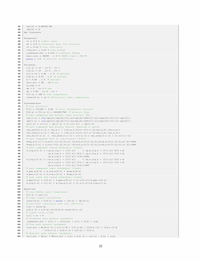
Appendix A. Batch Distillation Model344

The binary batch distillation column is represented by 42 constants, 252 variables, 595 explicit equations345

(intermediates), and 241 implicit differential and algebraic equations (DAEs). The equations are discretized346

over the startup (30 minutes) and measurement time horizon (60 minutes) with added objective to produce347

a final nonlinear programming problem with 11,972 equations and 11,976 variables (for the `1-norm). The348

following model in Listing 1 is expressed in the APMonitor Modeling Language. The software is freely avail-349

able at APMonitor.com as a Matlab, Python, or Julia package for dynamic simulation and optimization.350

This particular set of files can be accessed from the following GitHub archive [69].351

Listing 1: Binary Distillation Column Model in APMonitor Modeling Language3521 % Binary Batch D i s t i l l a t i o n Column353

2 % Component 1 = methanol354

3 % Component 2 = ethanol355

4 C o n s t a n t s356

5 n = 40 % stage s357

6 x 0 = 0.59 % i n i t i a l composit ion358

7 % Constants f o r heat o f vapor i za t i on359

8 A _ m = 3.2615 e 7360

9 B _ m = −1.0407361

10 C _ m = 1.8695362

11 D _ m = −0.60801363

12 A _ e = 6.5831 e 7364

13 B _ e = 1.1905365

14 C _ e = −1.7666366

15 D _ e = 1.0012367

16 % C r i t i c a l temperatures (K)368

17 T c _ m = 512.5369

18 T c _ e = 514370

19 % Density c o e f f i c i e n t s371

20 r h o _ m _ 1 = 2.3267372

21 r h o _ m _ 2 = 0.27073373

22 r h o _ m _ 3 = 512.05374

23 r h o _ m _ 4 = 0.24713375

24 r h o _ e _ 1 = 1.6288376

25 r h o _ e _ 2 = 0.27469377

26 r h o _ e _ 3 = 514378

27 r h o _ e _ 4 = 0.23178379

28 % Heat capac i ty c o e f f i c i e n t s380

29 c p _ m _ l i q _ 1 = 2.5604 E 5381

30 c p _ m _ l i q _ 2 = −2.7414 E 3382

31 c p _ m _ l i q _ 3 = 1.4777 E 1383

32 c p _ m _ l i q _ 4 = −3.5078 E−2384

33 c p _ m _ l i q _ 5 = 3.2719 E−5385

34 c p _ e _ l i q _ 1 = 1.0264 E 5386

35 c p _ e _ l i q _ 2 = −1.3963 E 2387

36 c p _ e _ l i q _ 3 = −3.0341 E−2388

37 c p _ e _ l i q _ 4 = 2.0386 E−3389

38 c p _ e _ l i q _ 5 = 0390

39 % Standard heats o f formation ( J/kmol )391

40 h _ f o r m _ s t d _ m = −2.391 E 8392

41 h _ f o r m _ s t d _ e = −2.7698 E 8393

42 % Vapor pre s su r e c o e f f i c i e n t s394

43 v p m [ 1 ] = 82.718395

44 v p m [ 2 ] = −6904.5396

45 v p m [ 3 ] = −8.8622397

46 v p m [ 4 ] = 7.4664 E−06398

47 v p m [ 5 ] = 2399

48 v p e [ 1 ] = 73.304400

49 v p e [ 2 ] = −7122.3401

50 v p e [ 3 ] = −7.1424402

21

51 v p e [ 4 ] = 2.8853 E−06403

52 v p e [ 5 ] = 2404

53 E n d C o n s t a n t s405

54406

55 P a r a m e t e r s407

56 r r = 3.5 % r e f l u x r a t i o408

57 h f = 0.8 % f r a c t i o n a l heat l o s s f r a c t i o n409

58 v f = 0.45 % tray e f f i c i e n c y410

59 t r a y _ h o l = 0.07 % tray holdup411

60 c o n d e n s e r _ h o l = 0.144 % condenser holdup412

61 h e a t _ r a t e = 36000 , > 0 % 36000 J/min = 600 W413

62 gamma = 1.0 % a c t i v i t y c o e f f i c i e n t414

63415

64 V a r i a b l e s416

65 x [ 1 : n ] = x 0 , >= 0 , <= 1417

66 y [ 2 : n ] = x 0 , >= 0 , <= 1418

67 L [ 1 : n −1] = 0.36 , > 0 % mol/min419

68 V [ 2 : n ] = 0.72 , > 0 % mol/min420

69 D = 0.36 , > 0 % mol/min421

70 b o i l _ h o l = 28 , >0 % mol422

71 Q _ c o n d = 0423

72 n p = 0 , >= 0 % mol424

73 x p = 0.99 , >= 0 , <= 1425

74 T [ 1 : n ] = 320 % tray temperature426

75 y s t a r [ 2 : n ] = x 0 % th e o r e t i c a l vapor composit ion427

76428

77 I n t e r m e d i a t e s429

78 % tray p r e s su r e s430

79 P [ 1 ] = 101325 ∗ 0 .86 % l o c a l atmospheric p re s su re431

80 P [ 2 : n ] = P [ 1 : n −1] + 101325/760 % pre s su re drop432

81 % pure component and mixture vapor pre s su re (Pa)433

82 v p 1 [ 1 : n ] = exp ( v p m [1 ]+ v p m [ 2 ] / T [ 1 : n ]+ v p m [ 3 ] ∗ L O G ( T [ 1 : n ] )+v p m [ 4 ] ∗ ( T [ 1 : n ] ˆ v p m [ 5 ] ) )434

83 v p 2 [ 1 : n ] = exp ( v p e [1 ]+ v p e [ 2 ] / T [ 1 : n ]+ v p e [ 3 ] ∗ L O G ( T [ 1 : n ] )+v p e [ 4 ] ∗ ( T [ 1 : n ] ˆ v p e [ 5 ] ) )435

84 v p [ 1 : n ] = x [ 1 : n ] ∗ v p 1 [ 1 : n ] + (1− x [ 1 : n ] ) ∗ v p 2 [ 1 : n ]436

85 % pure component and mixutre dens i ty ( kmol/m3 or mol/L)437

86 r h o _ m e t h [ 1 : n −1] = r h o _ m _ 1 / ( r h o _ m _ 2 ˆ(1+(1− T [ 1 : n −1]/ r h o _ m _ 3 ) ˆ r h o _ m _ 4 ) )438

87 r h o _ e t h a [ 1 : n −1] = r h o _ e _ 1 / ( r h o _ e _ 2 ˆ(1+(1− T [ 1 : n −1]/ r h o _ e _ 3 ) ˆ r h o _ e _ 4 ) )439

88 r h o _ m i x [ 1 : n −1] = r h o _ m e t h [ 1 : n −1] ∗ x [ 1 : n −1] + r h o _ e t h a [ 1 : n −1] ∗ (1− x [ 1 : n −1])440

89 % pure component heat o f vapor i za t i on ( J/mol )441

90 H v a p _ m [ 1 : n ] = A _ m ∗(1− T [ 1 : n ] / T c _ m ) ˆ( B _ m+C _ m ∗( T [ 1 : n ] / T c _ m )+D _ m ∗( T [ 1 : n ] / T c _ m ) ˆ2) /1000442

91 H v a p _ e [ 1 : n ] = A _ e ∗(1− T [ 1 : n ] / T c _ e ) ˆ( B _ e+C _ e ∗( T [ 1 : n ] / T c _ e )+D _ e ∗( T [ 1 : n ] / T c _ e ) ˆ2) /1000443

92 % pure component l i q u i d en tha lp i e s ( J/mol )444

93 h _ l i q _ m [ 1 : n ] = ( c p _ m _ l i q _ 1 ∗ ( T [ 1 : n ] ) + c p _ m _ l i q _ 2 ∗ ( T [ 1 : n ] ) ˆ2/2 + &445

94 c p _ m _ l i q _ 3 ∗ ( T [ 1 : n ] ) ˆ3/3 + c p _ m _ l i q _ 4 ∗ ( T [ 1 : n ] ) ˆ4/4 + &446

95 c p _ m _ l i q _ 5 ∗ ( T [ 1 : n ] ) ˆ5/5) /1000447

96 h _ l i q _ e [ 1 : n ] = ( c p _ e _ l i q _ 1 ∗ ( T [ 1 : n ] ) + c p _ e _ l i q _ 2 ∗ ( T [ 1 : n ] ) ˆ2/2 + &448

97 c p _ e _ l i q _ 3 ∗ ( T [ 1 : n ] ) ˆ3/3 + c p _ e _ l i q _ 4 ∗ ( T [ 1 : n ] ) ˆ4/4 + &449

98 c p _ e _ l i q _ 5 ∗ ( T [ 1 : n ] ) ˆ5/5) /1000450

99 % pure component vapor en tha lp i e s ( J/mol )451

100 h _ g a s _ m [ 2 : n ] = h _ l i q _ m [ 2 : n ] + H v a p _ m [ 2 : n ]452

101 h _ g a s _ e [ 1 : n ] = h _ l i q _ e [ 1 : n ] + H v a p _ e [ 1 : n ]453

102 % tray vapor and l i q u i d en tha lp i e s ( J/mol )454

103 h _ g a s [ 2 : n ] = y [ 2 : n ] ∗ h _ g a s _ m [ 2 : n ] + (1− y [ 2 : n ] ) ∗ h _ g a s _ e [ 2 : n ]455

104 h _ l i q [ 1 : n ] = x [ 1 : n ] ∗ h _ l i q _ m [ 1 : n ] + (1− x [ 1 : n ] ) ∗ h _ l i q _ e [ 1 : n ]456

105457

106 E q u a t i o n s458

107 % tray bubble point temperature459

108 P [ 1 : n ] = v p [ 1 : n ]460

109 % vapor l i q u i d equ i l i b r ium461

110 y s t a r [ 2 : n ] ∗ P [ 2 : n ] = gamma ∗ x [ 2 : n ] ∗ v p 1 [ 2 : n ]462

111 % non−i d e a l s epara t i on with tray e f f i c i e n c y463

112 y [ n ] = y s t a r [ n ]464

113 y [ 2 : n −1] = y [ 3 : n ]− v f ∗( y [ 3 : n ]− y s t a r [ 2 : n −1])465

114 % r e f l u x r a t i o = L/D466

115 L [ 1 ] = r r ∗ D467

116 % Condenser mole balance ( methanol )468

117 c o n d e n s e r _ h o l ∗ x [ 1 ] = − ( L [1 ]+ D ) ∗ x [ 1 ] + V [ 2 ] ∗ y [ 2 ]469

118 % Tray mole balance (methanol )470

119 t r a y _ h o l ∗ $x [ 2 : n −1] = L [ 1 : n −2] ∗ x [ 1 : n −2] − ( L [ 2 : n −1]) ∗ x [ 2 : n −1] &471

120 − V [ 2 : n −1] ∗ y [ 2 : n −1] + y [ 3 : n ] ∗ V [ 3 : n ]472

121 % Rebo i l e r mole balance (methanol )473

122 b o i l _ h o l ∗ $x [ n ] + $ b o i l _ h o l ∗ x [ n ] = L [ n −1] ∗ x [ n −1] − V [ n ] ∗ y [ n ]474

22

123 % Overa l l condenser mole balance475

124 V [ 2 ] = D ∗ ( r r+1)476

125 % Overa l l t ray mole balance477

126 0 = V [ 3 : n ] + L [ 1 : n −2] − V [ 2 : n −1] − L [ 2 : n −1]478

127 % Energy balance ( no dynamics )479

128 0 = ( V [ 2 ] ∗ ( h _ g a s [ 2 ] − h _ l i q [ 1 ] ) − Q _ c o n d )480

129 0 = V [ 3 : n ] ∗ ( h _ g a s [ 3 : n ] − h _ l i q [ 2 : n −1]) − V [ 2 : n −1] ∗ ( h _ g a s [ 2 : n −1] − h _ l i q [ 2 : n −1]) &481

130 − L [ 1 : n −2] ∗ ( h _ l i q [ 1 : n −2] − h _ l i q [ 2 : n −1])482

131 0 = h e a t _ r a t e ∗ h f − V [ n ] ∗ ( h _ g a s [ n ]− h _ l i q [ n ] ) − L [ n −1] ∗ ( h _ l i q [ n−1]− h _ l i q [ n ] )483

132 % Production ra te equat ions484

133 $ b o i l _ h o l = −D485

134 $ n p = D486

135 x p ∗ $ n p + n p ∗ $ x p = x [ 1 ] ∗ D487488

The following Python script shown in Listing 2 is the list of commands necessary to reproduce the489

dynamic batch distillation case presented in this paper. The parameter estimation uses two external files490

including the model file (distill.apm) and a data file (data.csv) that are also shown in this Appendix.491

Listing 2: Python Dynamic Estimation4921 f r o m a p m i m p o r t ∗493

2 s = ' http :// byu . apmonitor . com '494

3 a = ' d i s t i l l l 1 n o rm '495

4 a p m ( s , a , ' c l e a r a l l ' )496

5 a p m _ l o a d ( s , a , ' d i s t i l l . apm ' )497

6 c s v _ l o a d ( s , a , ' data . csv ' )498

7 a p m _ o p t i o n ( s , a , ' nlc . imode ' , 5 )499

8 a p m _ o p t i o n ( s , a , ' nlc . max iter ' ,100)500

9 a p m _ o p t i o n ( s , a , ' nlc . nodes ' , 2 )501

10 a p m _ o p t i o n ( s , a , ' nlc . t im e s h i f t ' , 0 )502

11 a p m _ o p t i o n ( s , a , ' nlc . ev type ' , 1 )503

12 a p m _ i n f o ( s , a , 'FV ' , ' hf ' )504

13 a p m _ i n f o ( s , a , 'FV ' , ' vf ' )505

14 a p m _ i n f o ( s , a , 'FV ' , ' t r ay ho l ' )506

15 a p m _ i n f o ( s , a , 'FV ' , ' condenser ho l ' )507

16 a p m _ i n f o ( s , a , 'CV ' , 'x [ 1 ] ' )508

17 a p m _ i n f o ( s , a , 'CV ' , 'np ' )509

18 o u t p u t = a p m ( s , a , ' s o l v e ' )510

19 pr in t ( o u t p u t )511

20 a p m _ o p t i o n ( s , a , ' hf . s t a tu s ' , 1 )512

21 a p m _ o p t i o n ( s , a , ' vf . s t a tu s ' , 1 )513

22 a p m _ o p t i o n ( s , a , ' t r ay ho l . s t a tu s ' , 1 )514

23 a p m _ o p t i o n ( s , a , ' condenser ho l . s t a tu s ' , 1 )515

24 a p m _ o p t i o n ( s , a , 'x [ 1 ] . f s t a t u s ' , 1 )516

25 a p m _ o p t i o n ( s , a , 'np . f s t a t u s ' , 1 )517

26 a p m _ o p t i o n ( s , a , 'x [ 1 ] . wsphi ' ,10000)518

27 a p m _ o p t i o n ( s , a , 'x [ 1 ] . wsplo ' ,10000)519

28 a p m _ o p t i o n ( s , a , 'np . wsphi ' ,10)520

29 a p m _ o p t i o n ( s , a , 'np . wsplo ' ,10)521

30 a p m _ o p t i o n ( s , a , 'x [ 1 ] . meas gap ' ,1 e−4)522

31 a p m _ o p t i o n ( s , a , 'np . meas gap ' , 0 . 0 1 )523

32 a p m _ o p t i o n ( s , a , ' hf . lower ' , 0 . 001 ) ;524

33 a p m _ o p t i o n ( s , a , ' hf . upper ' , 1 . 0 ) ;525

34 a p m _ o p t i o n ( s , a , ' vf . lower ' , 0 . 001 ) ;526

35 a p m _ o p t i o n ( s , a , ' vf . upper ' , 0 . 6 ) ;527

36 a p m _ o p t i o n ( s , a , ' t r ay ho l . lower ' , 0 . 01 ) ;528

37 a p m _ o p t i o n ( s , a , ' t r ay ho l . upper ' , 0 . 1 ) ;529

38 a p m _ o p t i o n ( s , a , ' condenser ho l . lower ' , 0 . 1 )530

39 a p m _ o p t i o n ( s , a , ' condenser ho l . upper ' , 0 . 5 )531

40 o u t p u t = a p m ( s , a , ' s o l v e ' )532

41 pr in t ( o u t p u t )533

42 y = a p m _ s o l ( s , a )534

43 pr in t ( ' hf : ' + s t r ( y [ ' hf ' ] [ −1 ] ) )535

44 pr in t ( ' vf : ' + s t r ( y [ ' vf ' ] [ −1 ] ) )536

45 pr in t ( ' t r ay ho l : ' + s t r ( y [ ' t r ay ho l ' ] [ −1 ] ) )537

46 pr in t ( ' cond hol : ' + s t r ( y [ ' condenser ho l ' ] [ −1 ] ) )538

23

47 pr in t ( 'np : ' + s t r ( y [ 'np ' ] [ −1 ] ) )539

48 pr in t ( 'xp : ' + s t r ( y [ 'xp ' ] [ −1 ] ) )540

49541

50 i m p o r t m a t p l o t l i b . p y p l o t a s p l t542

51 i m p o r t p a n d a s a s p d543

52 d a t a _ f i l e = p d . r e a d _ c s v ( ' da t a f o r p l o t t i n g . csv ' )544

53545

54 p l t . f i g u r e (1)546

55 p l t . subplot (3 ,1 , 1 )547

56 p l t . p l o t ( y [ ' time ' ] , y [ 'np ' ] , 'bx− ' , l i n e w i d t h =2.0)548

57 p l t . p l o t ( d a t a _ f i l e [ ' time ' ] , d a t a _ f i l e [ 'np ' ] , ' ro ' )549

58 p l t . l egend ( [ ' Predicted ' , 'Measured ' ] )550

59 p l t . y l abe l ( ' Moles ' )551

60552

61 a x = p l t . subplot (3 , 1 , 2 )553

62 p l t . p l o t ( y [ ' time ' ] , y [ 'x [ 1 ] ' ] , 'bx− ' , l i n e w i d t h =2.0)554

63 p l t . p l o t ( d a t a _ f i l e [ ' time ' ] , d a t a _ f i l e [ 'x [ 1 ] ' ] , ' ro ' )555

64 p l t . p l o t ( y [ ' time ' ] , y [ 'xp ' ] , 'k : ' , l i n e w i d t h =2.0)556

65 p l t . l egend ( [ ' Predicted ' , 'Measured ' , ' Cumulative ' ] )557

66 p l t . y l abe l ( ' Composition ' )558

67 a x . s e t _ y l i m ( [ 0 . 6 , 1 . 0 5 ] )559

68560

69 p l t . subplot (3 ,1 , 3 )561

70 p l t . p l o t ( y [ ' time ' ] , y [ 'x [ 1 ] ' ] , 'bx− ' , l i n e w i d t h =2.0)562

71 p l t . p l o t ( y [ ' time ' ] , y [ 'x [ 2 ] ' ] , 'k : ' , l i n e w i d t h =2.0)563

72 p l t . p l o t ( y [ ' time ' ] , y [ 'x [ 5 ] ' ] , ' r−− ' , l i n e w i d t h =2.0)564

73 p l t . p l o t ( y [ ' time ' ] , y [ 'x [ 1 0 ] ' ] , 'm.− ' , l i n e w i d t h =2.0)565

74 p l t . p l o t ( y [ ' time ' ] , y [ 'x [ 2 0 ] ' ] , 'y− ' , l i n e w i d t h =2.0)566

75 p l t . p l o t ( y [ ' time ' ] , y [ 'x [ 3 0 ] ' ] , 'g−. ' , l i n e w i d t h =2.0)567

76 p l t . p l o t ( y [ ' time ' ] , y [ 'x [ 4 0 ] ' ] , 'k− ' , l i n e w i d t h =2.0)568

77 p l t . l egend ( [ ' x1 ' , ' x2 ' , ' x5 ' , ' x10 ' , ' x20 ' , ' x30 ' , ' x40 ' ] )569

78 p l t . y l abe l ( ' Composition ' )570

79571

80 p l t . s a v e f i g ( ' r e s u l t s l 1 . png ' )572

81 p l t . s h o w ( )573574

The data file includes time, reflux ratio, the instantaneous product composition, and the total product575

moles. The data file includes the first 30 minutes with nearly infinite reflux when the batch column approaches576

a steady state. At 30 minutes, the reflux ratio is changed to collect dynamic data at regular intervals as577

shown in Table A.4.578

Figure A.12 shows the results of the `1-norm parameter estimation that are computed with the Python579

script in Listing 2. The first subplot shows the predicted and measured total moles. Note that the data580

collection starts after 30 minutes when the column is initially brought to steady state. The second and third581

subplots show the tray and product compositions. Over the first 30 minutes, there is insignificant total582

production. The product composition is below the 99% target but quickly reaches the desired purity once583

the reflux ratio is changed to allow production. Some of the individual tray compositions are shown in the584

final subplot. However, these compositions are not measured directly, only predicted from the model fit to585

the produced moles and product composition measurements.586

Appendix B. References587

[1] A. Lucia, B. R. McCallum, Energy targeting and minimum energy distillation column sequences, Com-588

puters & Chemical Engineering 34 (6) (2010) 931 – 942. doi:10.1016/j.compchemeng.2009.10.006.589

[2] P. Li, H. A. Garcia, G. Wozny, E. Reuter, Optimization of a semibatch distillation process with model590

24

Table A.4: Data File (data.csv) in Tabular Form

Time (s) Reflux Ratio Composition Product Moles

0 10000 x x

2.5 10000 x x

5 10000 x x

7.5 10000 x x

10 10000 x x

12.5 10000 x x

15 10000 x x

15.2 10000 x x

17.5 10000 x x

20 10000 x x

22.5 10000 x x

25 10000 x x

27.5 10000 x x

29.9 10000 x x

30.1 3.5 x x

32.5 3.5 0.991101728 0.590780164

35 3.5 0.999141476 1.060146

37.5 3.5 0.999141476 1.381291045

40 3.5 1.000195093 1.949735921

42.5 3.5 0.999773764 2.369812428

45 3.5 0.999984448 2.740502759

45.2 1 0.999984448 2.740502759

47.5 1 0.997875836 3.530570903

50 1 0.982790672 4.46255546

52.5 1 0.923087024 5.394604756

55 1 0.827170789 6.312827944

57.5 1 0.769688475 7.187411473

60 1 0.738080225 8.051023448

60.2 7 0.738080225 8.051023448

62.5 7 0.819332828 8.256959561

65 7 0.927134663 8.496361625

67.5 7 0.963811731 8.739591512

70 7 0.980221149 8.984573896

72.5 7 0.98940185 9.230547824

75 7 0.993222995 9.476936818

75.2 3.5 0.993222995 9.476936818

77.5 3.5 0.994282141 9.871343681

80 3.5 0.995763281 10.24134224

82.5 3.5 0.994705521 10.63582289

85 3.5 0.992162858 11.0298608

87.5 3.5 0.990039603 11.42352977

90 3.5 0.986847248 11.84121504

validation on the industrial site, Industrial & Engineering Chemistry Research 37 (4) (1998) 1341–1350.591

doi:10.1021/ie970695l.592

[3] S. Ulas, U. M. Diwekar, M. A. Stadtherr, Uncertainties in parameter estimation and optimal control593

in batch distillation, Computers & Chemical Engineering 29 (8) (2005) 1805 – 1814. doi:10.1016/j.594

compchemeng.2005.03.002.595

[4] K. Wang, T. Lohl, M. Stobbe, S. Engell, A genetic algorithm for online-scheduling of a multiproduct596

polymer batch plant, Computers & Chemical Engineering 24 (2) (2000) 393–400.597

[5] E. Robinson, The optimisation of batch distillation operations, Chemical Engineering Science 24 (11)598

(1969) 1661 – 1668. doi:10.1016/0009-2509(69)87031-4.599

[6] D. Mayur, R. May, R. Jackson, The time-optimal problem in binary batch distillation with a recycled600

25

0 10 20 30 40 50 60 70 80 9002468

1012

Moles

Predicted

Measured

0 10 20 30 40 50 60 70 80 900.60.70.80.91.0

Composition

Predicted

Measured

Cumulative

0 10 20 30 40 50 60 70 80 900.30.40.50.60.70.80.91.0

Composition

x1

x2

x5

x10

x20

x30

x40

Figure A.12: Results of the `1-norm Estimation with the Detailed Model

waste-cut, The Chemical Engineering Journal 1 (1) (1970) 15 – 21, the Chemical Engineering Journal.601

doi:10.1016/0300-9467(70)85026-2.602

[7] E. Robinson, The optimal control of an industrial batch distillation column, Chemical Engineering603

Science 25 (6) (1970) 921 – 928. doi:10.1016/0009-2509(70)85037-0.604

[8] W. L. Luyben, Some practical aspects of optimal batch distillation design, Industrial & Engineering605

Chemistry Process Design and Development 10 (1) (1971) 54–59. doi:10.1021/i260037a010.606

[9] Y.-S. Kim, Optimal control of time-dependent processes (design, batch distillation, catalyst deactiva-607

tion).608

[10] U. Diwekar, Batch Distillation: Simulation, Optimal Design, and Control, CRC Press, 1995.609

[11] B. T. Safrit, A. W. Westerberg, Improved operational policies for batch extractive distillation columns,610

Industrial & Engineering Chemistry Research 36 (2) (1997) 436–443. doi:10.1021/ie960343z.611

[12] K. H. Low, E. Srensen, Simultaneous optimal configuration, design and operation of batch distillation,612

AIChE Journal 51 (6) (2005) 1700–1713. doi:10.1002/aic.10522.613

[13] L. Bonny, Multicomponent batch distillations campaign: Control variables and optimal recycling policy,614

Industrial & Engineering Chemistry Research 45 (26) (2006) 8998–9009. doi:10.1021/ie0609057.615

26

[14] L. Bonny, Multicomponent batch distillations campaign: Control variables and optimal recycling policy.616

a further note, Industrial & Engineering Chemistry Research 52 (5) (2013) 2190–2193. doi:10.1021/617

ie3018302.618

[15] J. Kim, D. Ju, Multicomponent batch distillation with distillate receiver, Korean Journal of Chemical619

Engineering 20 (3) (2003) 522–527. doi:10.1007/BF02705559.620

[16] S.-S. Jang, Dynamic optimization of multicomponent batch distillation processes using continuous and621

discontinuous collocation polynomial policies, The Chemical Engineering Journal 51 (2) (1993) 83 – 92.622

doi:10.1016/0300-9467(93)80014-F.623

[17] V. A. Varma, G. V. Reklaitis, G. Blau, J. F. Pekny, Enterprise-wide modeling & optimizationan overview624

of emerging research challenges and opportunities, Computers & Chemical Engineering 31 (5) (2007)625

692–711.626

[18] C. Loeblein, J. Perkins, B. Srinivasan, D. Bonvin, Performance analysis of on-line batch optimization627

systems, Computers & Chemical Engineering 21 (1997) S867–S872.628

[19] H. Shi, F. You, A novel adaptive surrogate modeling-based algorithm for simultaneous optimization of629

sequential batch process scheduling and dynamic operations, AIChE Journal.630

[20] W. Dai, D. P. Word, J. Hahn, Modeling and dynamic optimization of fuel-grade ethanol fermentation631

using fed-batch process, Control Engineering Practice 22 (2014) 231–241.632

[21] Y. Chu, F. You, Integration of scheduling and dynamic optimization of batch processes under uncer-633

tainty: Two-stage stochastic programming approach and enhanced generalized benders decomposition634

algorithm, Industrial & Engineering Chemistry Research 52 (47) (2013) 16851–16869.635

[22] B. Srinivasan, S. Palanki, D. Bonvin, Dynamic optimization of batch processes: I. characterization of636

the nominal solution, Computers & Chemical Engineering 27 (1) (2003) 1–26.637

[23] T. Bhatia, L. T. Biegler, Dynamic optimization in the design and scheduling of multiproduct batch638

plants, Industrial & Engineering Chemistry Research 35 (7) (1996) 2234–2246.639

[24] P. Terwiesch, M. Agarwal, D. W. Rippin, Batch unit optimization with imperfect modelling: a survey,640

Journal of Process Control 4 (4) (1994) 238–258.641

[25] K. Kim, U. Diwekar, New era in batch distillation: Computer aided analysis, optimal design and control,642

Reviews in Chemical Engineering 17 (2) (2001) 111 – 164.643

[26] J. Stichlmair, J. R. Fair, Distillation: principles and practices, Vch Verlagsgesellschaft Mbh, 1998.644

[27] M. F. Doherty, M. F. Malone, Conceptual design of distillation systems, McGraw-Hill Science/Engi-645

neering/Math, 2001.646

27

[28] U. Diwekar, R. Malik, K. Madhavan, Optimal reflux rate policy determination for multicomponent647

batch distillation columns, Computers & Chemical Engineering 11 (6) (1987) 629 – 637. doi:10.1016/648

0098-1354(87)87008-4.649

[29] M. Barolo, G. Guarise, Batch distillation of multicomponent systems with constant relative volatilities,650

Chemical Engineering Research and Design 74 (8) (1996) 863 – 871. doi:http://dx.doi.org/10.651

1205/026387696523166.652

[30] Y. H. Kim, Optimal design and operation of a multi-product batch distillation column using dynamic653

model, Chemical Engineering and Processing: Process Intensification 38 (1) (1999) 61 – 72. doi:http:654

//dx.doi.org/10.1016/S0255-2701(98)00065-8.655

[31] I. Mujtaba, M. Hussain, Optimal operation of dynamic processes under process-model mismatches:656

Application to batch distillation, Computers & Chemical Engineering 22, Supplement 1 (1998) S621 –657

S624, european Symposium on Computer Aided Process Engineering-8. doi:http://dx.doi.org/10.658

1016/S0098-1354(98)00109-4.659

[32] S. Gruetzmann, G. Fieg, Startup operation of middle-vessel batch distillation column: modeling and sim-660

ulation, Industrial & Engineering Chemistry Research 47 (3) (2008) 813–824. doi:10.1021/ie070667v.661

[33] M. Hanke, P. Li, Simulated annealing for the optimization of batch distillation processes, Computers662

& Chemical Engineering 24 (1) (2000) 1 – 8. doi:http://dx.doi.org/10.1016/S0098-1354(00)663

00317-3.664

[34] M. Diehl, J. Gerhard, W. Marquardt, M. Mnnigmann, Numerical solution approaches for robust665

nonlinear optimal control problems, Computers & Chemical Engineering 32 (6) (2008) 1279 – 1292.666

doi:http://dx.doi.org/10.1016/j.compchemeng.2007.06.002.667

[35] V. Prasad, B. Bequette, Nonlinear system identification and model reduction using artificial neural668

networks, Computers & Chemical Engineering 27 (12) (2003) 1741 – 1754. doi:http://dx.doi.org/669

10.1016/S0098-1354(03)00137-6.670

[36] P. Li, H. P. Hoo, G. Wozny, Efficient simulation of batch distillation processes by using orthogo-671

nal collocation, Chemical Engineering & Technology 21 (11) (1998) 853–862. doi:10.1002/(SICI)672

1521-4125(199811)21:11<853::AID-CEAT853>3.0.CO;2-2.673

[37] S. Jain, J.-K. Kim, R. Smith, Operational optimization of batch distillation systems, Industrial &674

Engineering Chemistry Research 51 (16) (2012) 5749–5761. doi:10.1021/ie201844g.675

[38] M. Leipold, S. Gruetzmann, G. Fieg, An evolutionary approach for multi-objective dynamic optimization676

applied to middle vessel batch distillation, Computers & Chemical Engineering 33 (4) (2009) 857 – 870.677

doi:http://dx.doi.org/10.1016/j.compchemeng.2008.12.010.678

28

[39] L. Biegler, X. Yang, G. Fischer, Advances in sensitivity-based nonlinear model predictive control and679

dynamic real-time optimization, Journal of Process Control (2015) –doi:http://dx.doi.org/10.1016/680

j.jprocont.2015.02.001.681

[40] A. Bonsfills, L. Puigjaner, Batch distillation: simulation and experimental validation, Chemical Engi-682

neering and Processing: Process Intensification 43 (10) (2004) 1239 – 1252. doi:10.1016/j.cep.2003.683

11.009.684

[41] M. Barolo, F. Botteon, Calculation of parametric sensitivity in binary batch distillation, Chemical685

Engineering Science 53 (10) (1998) 1819 – 1834. doi:http://dx.doi.org/10.1016/S0009-2509(98)686

00017-7.687

[42] A. O. Converse, G. D. Gross, Optimal distillate-rate policy in batch distillation, Industrial & Engineering688

Chemistry Fundamentals 2 (3) (1963) 217–221. doi:10.1021/i160007a010.689

[43] M. M. Lopes, T. W. Song, Batch distillation: Better at constant or variable reflux?, Chemical Engi-690

neering and Processing: Process Intensification 49 (12) (2010) 1298 – 1304. doi:http://dx.doi.org/691

10.1016/j.cep.2010.09.019.692

[44] J. V. Beck, K. J. Arnold, Parameter estimation in engineering and science, James Beck, 1977.693

[45] S. Wu, K. A. McLean, T. J. Harris, K. B. McAuley, Selection of optimal parameter set using estimabil-694

ity analysis and MSE-based model-selection criterion, International Journal of Advanced Mechatronic695

Systems 3 (3) (2011) 188–197. doi:10.1504/IJAMECHS.2011.042615.696

[46] B. Srinivasan, D. Bonvin, E. Visser, S. Palanki, Dynamic optimization of batch processes: Ii. role of697

measurements in handling uncertainty, Computers & Chemical Engineering 27 (1) (2003) 27–44.698

[47] S. M. Safdarnejad, J. D. Hedengren, L. L. Baxter, L. Kennington, Investigating the impact of cryogenic699

carbon capture on the performance of power plants, in: Proceedings of the American Control Conference700

(ACC), Chicago, IL, 2015, pp. 5016–5021. doi:10.1109/ACC.2015.7172120.701

[48] K. M. Powell, J. D. Hedengren, T. F. Edgar, Dynamic optimization of a hybrid solar thermal and fossil702

fuel system, Solar Energy 108 (2014) 210 – 218. doi:http://dx.doi.org/10.1016/j.solener.2014.703

07.004.704

[49] K. M. Powell, J. D. Hedengren, T. F. Edgar, Dynamic optimization of a solar thermal energy storage705

system over a 24 hour period using weather forecasts, in: American Control Conference (ACC), 2013,706

IEEE, 2013, pp. 2946–2951.707

[50] S. M. Safdarnejad, J. D. Hedengren, N. R. Lewis, E. L. Haseltine, Initialization strategies for opti-708

mization of dynamic systems, Computers & Chemical Engineering 78 (2015) 39 – 50. doi:10.1016/j.709

compchemeng.2015.04.016.710

29

[51] J. D. Hedengren, APMonitor Modeling Language, http://www.apmonitor.com, (accessed November711

2015).712

[52] B. J. Spivey, J. D. Hedengren, T. F. Edgar, Constrained nonlinear estimation for industrial process713

fouling, Industrial & Engineering Chemistry Research 49 (17) (2010) 7824–7831.714

[53] R. Asgharzadeh Shishavan, C. Hubbell, H. Perez, J. Hedengren, D. Pixton, Combined rate of penetra-715

tion and pressure regulation for drilling optimization by use of high-speed telemetry, SPE Drilling &716

Completion (SPE-170275-PA). doi:10.2118/170275-PA.717

[54] J. D. Hedengren, R. A. Shishavan, K. M. Powell, T. F. Edgar, Nonlinear modeling, estimation and718

predictive control in APMonitor, Computers & Chemical Engineering 70 (2014) 133 – 148. doi:10.719

1016/j.compchemeng.2014.04.013.720

[55] G. Seber, C. Wild, Nonlinear Regression, John Wiley & Sons, Inc., Hoboken, New Jersey.721

[56] N. R. Lewis, J. D. Hedengren, E. L. Haseltine, Hybrid dynamic optimization methods for systems722

biology with efficient sensitivities, Processes 3 (3) (2015) 701. doi:10.3390/pr3030701.723

URL http://www.mdpi.com/2227-9717/3/3/701724

[57] Z. K. Nagy, R. D. Braatz, Worst-case and distributional robustness analysis of finite-time control tra-725

jectories for nonlinear distributed parameter systems, Control Systems Technology, IEEE Transactions726

on 11 (5) (2003) 694–704.727

[58] P. N. Brown, A. C. Hindmarsh, L. R. Petzold, Using krylov methods in the solution of large-scale728

differential-algebraic systems, SIAM Journal on Scientific Computing 15 (6) (1994) 1467–1488.729

[59] Y. Cao, S. Li, L. Petzold, R. Serban, Adjoint sensitivity analysis for differential-algebraic equations:730

The adjoint dae system and its numerical solution, SIAM Journal on Scientific Computing 24 (3) (2003)731

1076–1089.732

[60] J. Renfro, A. Morshedi, O. Asbjornsen, Simultaneous optimization and solution of systems described733

by differential/algebraic equations, Computers and Chemical Engineering 11 (5) (1987) 503 – 517.734

doi:10.1016/0098-1354(87)80025-X.735

[61] L. Sun, J. D. Hedengren, R. W. Beard, Optimal trajectory generation using model predictive control736

for aerially towed cable systems, Journal of Guidance, Control, and Dynamics 37 (2) (2014) 525–539.737

doi:10.2514/1.60820.738

[62] J. Tolsma, P. I. Barton, DAEPACK: An open modeling environment for legacy models, Industrial &739

Engineering Chemistry Research 39 (6) (2000) 1826–1839.740

30

[63] J. T. Leppavuori, M. M. Domach, L. T. Biegler, Parameter estimation in batch bioreactor simulation us-741

ing metabolic models: Sequential solution with direct sensitivities, Industrial & Engineering Chemistry742

Research 50 (21) (2011) 12080–12091. doi:10.1021/ie201020g.743

[64] S. M. Safdarnejad, J. D. Hedengren, L. L. Baxter, Plant-level dynamic optimization of cryogenic carbon744

capture with conventional and renewable power sources, Applied Energy 149 (2015) 354 – 366. doi:745

http://dx.doi.org/10.1016/j.apenergy.2015.03.100.746

[65] Chemcad version 6.5.0, owned by Chemstations, Inc. in Houston, TX. Copyright 2015.747

[66] R. L. Rowley, W. V. Wilding, J. L. Oscarson, T. A. Knotts, N. F. Giles, DIPPR data compilation of748

pure chemical properties, Design Institute for Physical Properties, AIChE, New York, NY, 2013.749

[67] J. D. Seader, E. J. Henley, Separation Process Principles, John Wiley & Sons, 2006.750

[68] J. D. Hedengren, A. N. Eaton, Overview of estimation methods for industrial dynamic systems, Opti-751

mization and Engineeringdoi:10.1007/s11081-015-9295-9.752

[69] J. D. Hedengren, APMonitor Modeling Language: Batch Distillation Files, https://github.com/753

APMonitor/batch_distillation, (accessed November 2015).754

31