Embed Size (px)
Citation preview

INFORMS 2010 c© 2010 INFORMS | isbn 978-0-9843378-0-4doi 10.1287/educ.1100.0077
Dynamic Optimization with Applications toDynamic Rate Queues
Robert C. HampshireSchool of Public Policy and Management, H. John Heinz III College, Carnegie Mellon University,Pittsburgh, Pennsylvania 15213, [email protected]
William A. MasseyOperations Research and Financial Engineering Department, Princeton University,Princeton, New Jersey 08540, [email protected]
Abstract This tutorial presents recent developments in the management of communicationsservices and applies broadly to services involving the leasing of shared resources. Theseproblems are more realistically modeled by queues with time-varying rates or moresimply, dynamic rate queues. We first provide a review and summary of relevant resultsfor various fundamental dynamic rate queues. The focus here is on approximations ofthese queueing models by low-dimensional dynamical systems.
The dynamic optimization of constrained dynamical systems is based on the calcu-lus of variations and its various incarnations over the past three centuries. We discussthese methods in the context of Lagrangians, Hamiltonians, and Bellman value func-tions. Finally, we provide examples where we apply these optimization techniques todynamic rate queues motivated by communications decision problems.
Keywords Bellman value function; calculus of variations; conservation principles; differen-tial equations; dynamical systems; Hamiltonian; Lagrangian; Lagrange multipliers;Legendre transforms; opportunity costs; optimal control; Poisson brackets
1. The Operations of Communication Systems and Services
1.1. Four Canonical IssuesWe begin by discussing the operational issues motivated by the communications industry.This is the business sector that created the telephone network in the beginning of the 20thcentury and gave birth to the mathematical field of queueing theory. Around the middleof the 20th century, or the 1960s, queueing theory was found to have applications to thecommunication of computer systems. The mathematics of queueing has taken on a life of itsown since then and has applications to all services involving the leasing of shared resources.A manager of a communications business has a continual interest in offering various ser-
vices as efficiently as possible in terms of the company resources. We can express theseconcerns in terms of four canonical issues: performance, pricing, provisioning, and priori-tization. The first one is that of service performance. These are metrics that predict theavailability of resources needed for service to the typical, newly arriving customer. This isexpressed in terms of the past demand and usage of these resources by previous customers.The second issue is service pricing. If the price is too high, then no one may use the
service. If the price is too low, then the cost of the resources used by the business providingthe service may exceed the revenue obtained. A decision must be made as to what is themost strategic price in terms of optimizing revenue without compromising some target levelof service performance. If the general strategy for a decision can be expressed in terms ofa finite set of simple steps, then we call this a policy. Since the larger goal of operations
208
INFORMS
holds
copyrightto
this
article
and
distrib
uted
this
copy
asa
courtesy
tothe
author(s).
Add
ition
alinform
ation,
includ
ingrig
htsan
dpe
rmission
policies,
isav
ailableat
http://journa
ls.in
form
s.org/.

Hampshire and Massey: Dynamic OptimizationTutorials in Operations Research, c© 2010 INFORMS 209
research is to make a strategic decision, our ultimate objective is to determine an optimalpolicy.The third issue is resource provisioning. This is the efficient design of the system so that
just enough or an optimal number of resources are made available to achieve an acceptabletarget level of service performance. Here again, a policy must be developed to determinethis critical amount.Finally, there is the issue of resource prioritization. This is the efficient allocation of
resources to distinct classes of customers. An optimal policy is one that accounts for thediffering levels of demand, performance needs, and payment for services by these differingclasses of customers.The issue of service performance calls for managers to assume a passive role. They need
only observe the history of the system to make their predictions. Classically, queueing the-ory has studied the static steady-state behavior of constant rate queues. We typically modelthese systems by time-homogeneousMarkov processes. However, these models fail to captureeveryday dynamic rate queueing phenomena such as the lag between the time of the peakdemand for services and the time of the peak load. It is the latter time and not the formerwhen the largest amount of service resources are needed. Hence to make more accurateperformance predictions, we need to study dynamic rate queues. The underlying mathe-matics for these models come from the study of time-inhomogeneous Markov processes anddynamical systems.Moreover, the remaining three issues of pricing, provisioning, and prioritization all require
an active role on the part of the managers to develop optimal policies. To analyze theseproblems, we model the forecasted demands for these services as random counting processes.We model the resulting communication service usage as a dynamic rate queue. In turn, wemodel these queueing systems as discrete state Markov processes. Assuming a deterministicinitial load and a finite time horizon makes the underlying Markov process transient, evenif it is time homogeneous. Our goal is to develop optimal policies by applying dynamicoptimization to these processes.Finding such optimal policies can be difficult if not computationally intractable. Our
approach is to develop an approximate analysis by optimizing deterministic dynamical sys-tems that are good approximations of the given Markov process queueing models. Theapproximate dynamic optimization policies developed here for queueing models result inopen-loop controls that depend on time and the parameters of the problem. In special casesfeedback or closed-loop controls may be obtained. However, this tutorial focuses on open-loop controls.
1.2. Literature ReviewThere is a vast literature in operations research relating to sequential decision making underuncertainty. We do not attempt to survey or cite all these works here. We merely point toa few streams that relate to the present tutorial and the control of dynamic rate queues.There is a large and growing stream of research on the control of queueing systems that
considers the exact optimization of steady-state queueing systems over an infinite time hori-zon. Sennott’s book [45] examines the control of queueing systems using stochastic dynamicprogramming. The textbooks of Puterman [43] and Bertsekas [5], among others, provide thefoundation for using Markov decision processes (MDP) for the exact optimization of station-ary queueing systems. Miller [39] provides optimality conditions for finite horizon continuoustime MDP with finite action spaces. There are many researchers who have extended theMDP framework to develop policies for nonhomogeneous stochastic models with infiniteactions spaces. As an example of this stream, Lewis and Yoon [31] consider both pricingand admission controls for a multiserver queue with a periodic arrival rate over an infinitetime horizon. They use a pointwise stationary approximation (PSA) of the queueing process(see Green and Kolesar [12]). An optimization problem is then solved over each disjoint
INFORMS
holds
copyrightto
this
article
and
distrib
uted
this
copy
asa
courtesy
tothe
author(s).
Add
ition
alinform
ation,
includ
ingrig
htsan
dpe
rmission
policies,
isav
ailableat
http://journa
ls.in
form
s.org/.

Hampshire and Massey: Dynamic Optimization210 Tutorials in Operations Research, c© 2010 INFORMS
time interval where stationarity is assumed. Additionally, the work of Fu et al. [11] con-siders the staffing of a transient queue using a pointwise stationary approximation and anonhomogeneous MDP.Another stream of work develops finite horizon analysis and approximations for nonho-
mogeneous MDP. A series of papers by Alden and Smith [2], Bean et al. [3], Hopp [21], andHopp et al. [22] develop optimality conditions and rolling horizon methods for nonhomoge-neous MDP.We focus on the approximate dynamic optimization of dynamic rate queues over a finite
time horizon. This tutorial summarizes the stream of research that uses dynamic systemsto model the service system and optimal control theory to perform the optimization. Anexample of a paper in this stream is the work of Agnew [1], who considers dynamic controlfor congestion prone systems. The authors have employed the methods developed in thistutorial in a series of papers (Hampshire [14], Hampshire et al. [18, 19]).
2. Fundamental Dynamic Rate QueuesIn this section we give a brief summary of queueing theory from a communications per-spective. The first queueing paper is said to have been written in 1917 by Erlang [7] todetermine the blocking probability (“all circuits are busy”) for telephone trunk lines. Anatural historical motivation for the field is to organize queueing models into the followingfour fundamental types: service demand models, revenue demand models, loss models, anddelay models.
2.1. Service Demand ModelsService demand is analyzed through the study of arrival traffic models where we simplycount the number of customers making service requests. For dynamic rates, we can start withthe following simple assumptions for an arrival process. We define a process A(t) | t≥ 0in terms of a positive, deterministic function λ(t) | t≥ 0, where
(1) We have a simple (unit jump) random counting process A(t) | t≥ 0.(2) The mean number of jumps in a time interval (s, t] is
∫ tsλ(r)dr.
(3) The random numbers of jumps during disjoint times intervals are mutually indepen-dent random variables.
By a theorem due to Prekopa [42], these assumptions uniquely characterize a nonhomoge-neous Poisson process, where
PA(t)−A(s) = n= exp(
−∫ t
s
λ(r)dr)(∫ tsλ(r)dr)n
n!,
for all integers n ≥ 0. If we view customers as a large population of independent actors,then these three assumptions are reasonable modeling assumptions. This makes the Poissonprocess a natural model for service demand traffic. The only adjustment that needs to bemade from the perspective of classical queueing theory is to consider nonhomogeneous aswell as homogeneous Poisson processes.
2.2. Service Resource Demand ModelsService resource demand is the total amount of service resources that are requested bythe customers at any given time. Communication examples of such resources are telephonetrunk lines, radio channels, bandwidth, or call center agents. The simplest service resourcedemand queueing models are ones with nonhomogeneous Poisson arrivals and an infinitenumber of servers where the service time is the service resource. Since the resources thatcustomers request are not necessarily the same as the resources they actually receive, we
INFORMS
holds
copyrightto
this
article
and
distrib
uted
this
copy
asa
courtesy
tothe
author(s).
Add
ition
alinform
ation,
includ
ingrig
htsan
dpe
rmission
policies,
isav
ailableat
http://journa
ls.in
form
s.org/.

Hampshire and Massey: Dynamic OptimizationTutorials in Operations Research, c© 2010 INFORMS 211
can model these requests as a sequence of independent and identically distributed, positiverandom variables. In classical telephony, this type of service demand is referred to as theoffered load.For the resulting offered load process Q∞(t) | t≥ 0, each Q∞(t) has a Poisson distribu-
tion or
PQ∞(t) = n= e−q∞(t) · q∞(t)n
n!for all positive integers n, including zero. However, this offered load process is not a Poissonprocess. As discussed in Eick et al. [6], the resulting deterministic, mean offered load processq∞(t) | t≥ 0 equals
q∞(t)≡E
[∫ t
t−S
λ(r)dr]=E [λ(t−Se)] ·E [S] ,
where the random variable S has the same distribution as any of the i.i.d. service times.The random variable Se is defined to have a stationary excess distribution from S, where
PSe ≤ t ≡ 1E[S]
∫ t
0PS > sds.
This is the distribution for the remaining time of an interrupted service from a renewalprocess for these i.i.d. times. If S has a finite second moment, then Se has a finite meanwhere
E [Se] =E[S2]2 ·E[S]
.
It can be shown that the distributions for S and Se are the same if and only if S isexponentially distributed or
Sed= S if and only if PS > t= e−µt where E[S] = 1/µ.
From the properties of the Poisson distribution, it follows that E [Q∞(t)] = q∞(t) for allt≥ 0. We can make this offered load process Markov by letting the service times (the amountof time customers are in service) have an exponential distribution with mean rate µ. Themean offered load q∞(t) | t≥ 0 then solves the ordinary differential equation
d
dtq∞(t) = λ(t)−µ · q∞(t).
Observe that for the case of λ being a constant, we have
limt→∞ q∞(t) = ρ≡ λ/µ.
For the time-homogeneous case, ρ equals the steady-state mean offered load.
2.3. Service Loss ModelsInspired by voice communications, service loss models are one way to handle the reality oflimited resources. Customers who arrive when there are no available service resources aretold to go away. In telephony, this is the experience of receiving the message that all circuitsare busy. For the case of a constant rate or time-homogeneous Poisson arrival process anda finite number of C servers, we have the classical Erlang loss model or M/M/C/C queue.The long run steady-state probability of all circuits being busy is given by βC(ρ), defined as
βC(ρ)≡ ρC
C!
/ C∑i=0
ρi
i!,
where ρ is the steady-state mean offered.
INFORMS
holds
copyrightto
this
article
and
distrib
uted
this
copy
asa
courtesy
tothe
author(s).
Add
ition
alinform
ation,
includ
ingrig
htsan
dpe
rmission
policies,
isav
ailableat
http://journa
ls.in
form
s.org/.

Hampshire and Massey: Dynamic Optimization212 Tutorials in Operations Research, c© 2010 INFORMS
Using the theory of time-reversible Markov processes (see Kelly [27]), we can also showthat
βC(ρ) = limt→∞PQC/C(t) =C= lim
t→∞PQ∞(t) =C |Q∞(t)≤C .
In general, the steady-state distribution for the Erlang loss system is the steady-state dis-tribution for the offered load system conditioned on being less than or equal to the numberof servers C. Because of the insensitivity results for the Erlang loss model in steady state,these steady-state distributional results extend to the non-Markovian case of general servicedistributions.For the case of nonhomogeneous Poisson arrivals, however, the transient probability of
blocking for the Erlang loss model no longer has this conditional Poisson distribution. Thisis true despite the fact that its offered load counterpart still has a Poisson distribution.Regardless, this conditional Poisson distribution is still a good estimation of the transientdistribution for the Erlang loss model and this technique is called the modified offered loadapproximation (see Jagerman [24] as well as Massey and Whitt [37]).We can still use the dynamical system of the mean offered load for approximating the
performance of the loss system queueing model, if we constrain the dynamical system tostay below some given threshold value. In practice, given C and 0< ε < 1, we need to findthe mean offered load value θ, where
βC(θ) = ε.
The modified offered load approximation then tells us that the dynamics of the event,
max0≤t≤T
PQC/C(t) =C ≤ ε,
can be estimated by the approximating event of
max0≤t≤T
q∞(t)≤ θ.
2.4. Service Delay ModelsService delay models, as inspired by data communications, are another way to handle theallocation of scarce resources. The customers that arrive when the necessary resources are notavailable for service are told to wait until the resources are available. An example is the delayexperienced when downloading a file from a Web server that is heavily used. Kleinrock [28]showed that a single server queue with a processor sharing (PS) service discipline couldapproximate the performance of CPU server with a round robin service discipline. Now letthe constant λ be the Poisson arrival rate and the constant 1/µ be the average size foran exponentially distributed job size for the queueing process QPS
1/∞(t) | t≥ 0. Using thetheory for steady-state distributions of Markov chains and processes gives us
limt→∞PQPS
1/∞(t) = n=(1− ρ)ρn if ρ < 1,0 if ρ≥ 1.
The PS service discipline has a natural scale invariance that leaves service timesunchanged. If we set η equal to a positive integer, then dividing each job into η even partsand processing these jobs in parallel does not change the processing time of the collectiveoriginal job. The η-fold i.i.d. superposition of nonhomogeneous Poisson arrivals with ratefunction λ(t) yields a nonhomogeneous Poisson process with rate function η · λ(t). Jobswhose size is exponentially distributed with rate µ are then exponentially distributed withrate η ·µ when divided by the scale factor η. This is a motivation for the asymptotic analysis
INFORMS
holds
copyrightto
this
article
and
distrib
uted
this
copy
asa
courtesy
tothe
author(s).
Add
ition
alinform
ation,
includ
ingrig
htsan
dpe
rmission
policies,
isav
ailableat
http://journa
ls.in
form
s.org/.

Hampshire and Massey: Dynamic OptimizationTutorials in Operations Research, c© 2010 INFORMS 213
of uniform acceleration for time-inhomogeneous Markov processes (see Massey [35] and laterMassey and Whitt [38]).If we let QPS
1/∞(t;η) | t≥ 0 be this newly scaled queueing process, then we have
limη→∞PQPS
1/∞(t;η) = n=(1− ρ(t))ρ(t)n if ρ∗(t)< 1,0 if ρ∗(t)≥ 1,
where
ρ(t)≡ λ(t)/µ and ρ∗(t)≡ sup0≤s<t
∫ tsλ(r)dr
µ · (t− s).
A proof of this result can be found in both Massey [35, 36]. The PS interpretation of uniformacceleration is discussed in Hampshire et al. [17].Through the theory of strong approximations (see Kolmos et al. [29], Ethier and Kurtz
[8]), we can also apply these same uniform acceleration asymptotics directly to the randomsample path behavior of this queueing process and obtain
limη→∞ sup
0≤t≤T
∣∣∣∣1ηQPS1/∞(t;η)− qPS1/∞(t)
∣∣∣∣= 0 a.s.,
where if qPS1/∞(0) = 0, then
qPS1/∞(t)≡ max0≤t≤T
∫ T
t
(λ(s)−µ)ds.
The resulting deterministic process qPS1/∞(t) | t ≥ 0 is called the fluid approximation forsingle server queues as discussed in Kleinrock [28]. The proof of this functional strong lawof large numbers is given in Mandelbaum and Massey [32]. Note that the fluid model is alsoa nonsmooth dynamical system of the form
d
dtqPS1/∞(t) = (λ(t)−µ) · qPS1/∞(t)> 0+(λ(t)−µ)+ · qPS1/∞(t) = 0,
where qPS1/∞(0) = 0. The term qPS1/∞(t)> 0 is a binary valued indicator function that hasthe value one if qPS1/∞(t)> 0 is true and zero otherwise.Another simple example of delay is in a telephone call where customers are hearing music
instead of a message that all circuits are busy. This can be modeled by a multiserver queuewith nonhomogeneous Poisson arrivals, an infinite capacity waiting space, and a first-come,first-served (FCFS) customer service discipline. The number of servers maps C to the numberof telephone call center agents. From a managerial perspective, a natural asymptotic analysisis to scale up the average rate of arriving customers from λ to η ·λ, where η > 1, and scalethe number of servers from C to η ·C. We are simultaneously scaling up the “supply” ofservice resources and the “demand” of the customer arrival rate. Such a scaling, in thelanguage of call centers, is called resource pooling. It was first considered asymptoticallyby Halfin and Whitt [13], and this type of scaling is defined to be in the quality efficiencydriven (QED) regime according to Zeltyn and Mandelbaum [47]. Dividing out this newMarkov process by this same scaling parameter η makes the resulting ratio converge to adeterministic dynamical system qFCFSC/∞ (t) | t≥ 0, where
limη→∞ sup
0≤t≤T
∣∣∣∣1ηQFCFSC/∞ (t;η)− qFCFSC/∞ (t)
∣∣∣∣= 0 a.s.
INFORMS
holds
copyrightto
this
article
and
distrib
uted
this
copy
asa
courtesy
tothe
author(s).
Add
ition
alinform
ation,
includ
ingrig
htsan
dpe
rmission
policies,
isav
ailableat
http://journa
ls.in
form
s.org/.

Hampshire and Massey: Dynamic Optimization214 Tutorials in Operations Research, c© 2010 INFORMS
with
d
dtqFCFSC/∞ (t) = λ(t)−µ ·min(qFCFSC/∞ (t),C)
and qFCFSC/∞ (0)≡QFCFSC/∞ (0). This new variant or QED version of uniform acceleration applies
to a large class of Markov processes that we call Markovian service networks. As was shownin Mandelbaum et al. [33], all networks of this type have a strong law of large numbers limittheorem when uniformly accelerated. Moreover, the limiting deterministic process is alwaysa dynamical system.Finally, we revisit the single server with the PS service discipline. This time we add a
permanent job that interacts with all the other jobs being processed. We can use this processto model the response time for a tagged customer entering the system at some specific timeand denote this service discipline by PS+. As shown in Hampshire and Massey [16], thissystem also fits into the framework of being a Markovian service network. The result isalmost sure convergence, uniformly on compact intervals of time, or
limη→∞ sup
0≤t≤T
∣∣∣∣1ηQPS+1/∞(t;η)− qPS+1/∞(t)
∣∣∣∣= 0 a.s.
to the deterministic dynamical system qPS+1/∞(t) | t≥ 0, which is uniquely characterized byits initial value and the ordinary differential equation
d
dtqPS+1/∞(t) = λ(t)−
µ · qPS+1/∞(t)
1+ qPS+1/∞(t).
2.5. Resource Demand DynamicsA recurring theme in dynamic rate queues is that the time of the peak arrival rate is not thetime of the peak mean offered load. The timing of the latter always has a positive lag afterthe timing of the former. A similar lag occurs for the times of the minimum arrival rate andthe minimal mean offered load. We can illustrate through an example this phenomena withthe dynamical system for the mean offered load.We can visualize the time evolution of this mean offered load q∞(t) | t≥ 0 by viewing
it as a one-dimensional dynamical system. In Figure 1, we make a phase-space plot of thetime derivative for q∞(t) versus its own time derivative for all time t≥ 0. For constant λ,we have a continuous evolution of the dynamical system along the phase-space equation ofa line, according to the ordinary differential equation. This line has λ as its y-intercept and−µ as its slope. When the time derivative of q∞(t) is positive, then the flow is toward theright or is increasing over time along the x-axis, when the line for the dynamical system flowis above the x-axis. Conversely, the system flow is from right to left when the flow line isbelow the x-axis. The phase-space plot reveals that all solutions to the differential equation(i.e., regardless of the initial value q∞(0)) converge to ρ= λ/µ as t goes to infinity.
When λ is time dependent, then the time evolution of the mean offered load process isno longer along a straight line. Moreover, the limit of q∞(t) as t approaches infinity may nolonger converge to a unique point in phase space. Suppose that we let the arrival rate of λbe periodic, we can show that the limiting behavior of q∞ is also periodic over time. Moreinformally, if the period is a “day,” then we have “time of day” limits for what we call theperiodic steady-state distribution.Now consider the following example from Horne et al. [23]. When we set λ(t) = a+ a ·sin(bt)
with b > 0, then the periodic steady-state behavior of the mean offered load phase-spaceprocess moves in a clockwise elliptical orbit as shown in Figure 2. The center of this closedcurve is at (a/µ,0). Moreover, the ellipse has both foci on the x-axis with extremal radiiequal to a/
√b2+µ2 and ab/
√b2+µ2. If we draw a line of slope −µ through any point on
INFORMS
holds
copyrightto
this
article
and
distrib
uted
this
copy
asa
courtesy
tothe
author(s).
Add
ition
alinform
ation,
includ
ingrig
htsan
dpe
rmission
policies,
isav
ailableat
http://journa
ls.in
form
s.org/.

Hampshire and Massey: Dynamic OptimizationTutorials in Operations Research, c© 2010 INFORMS 215
Figure 1. Phase-space plot of the mean offered load dynamical system with a constant arrivalrate.
(/,0)
(0,)
(q (0),0)
q
dqSlope – dt
the phase-space curve, then the y-intercept of the line gives the value of the arrival rate λat the time of the phase-space point.Now we show how our service resource demand model can help us manage a resource
provisioning problem for our service loss model. First, we define
C∗(ε, ρ)≡minC |βC(ρ)≤ ε.The integer value C∗(ε, ρ) equals the smallest number of servers needed such that theErlang blocking formula is less than or equal to ε for the given steady-state mean offeredload of ρ. The modified offered load approximation says that the scheduling policy ofC(t) |0≤ t≤ T , where
C(t)≡C∗(ε, q∞(t))
is a good estimate of the smallest number of servers needed to keep the blocking probabilitybelow ε over the interval (0, T ]. Hampshire et al. [20] develop this approach in the contextof bandwidth trading.
Figure 2. Phase-space plot of the mean offered load dynamical system with a sinusoidal arrivalrate.
(qmin,0)
(0,a+a)
(qmax,0)(a/,0)
dq
q2ab
2a
b2 + 2
b2 + 2
Slope –
dt
(0,a -a)
ˆ
ˆ
ˆ
ˆ
(0,a)
INFORMS
holds
copyrightto
this
article
and
distrib
uted
this
copy
asa
courtesy
tothe
author(s).
Add
ition
alinform
ation,
includ
ingrig
htsan
dpe
rmission
policies,
isav
ailableat
http://journa
ls.in
form
s.org/.
Hampshire and Massey: Dynamic Optimization216 Tutorials in Operations Research, c© 2010 INFORMS
2.6. Fundamental Decision ProblemsWe now introduce specific types of decision problems for dynamic rate queues that aremotivated by more than just optimizing the performance of the queueing model. Supposethat we want to develop a dynamic pricing policy π(t) |0 ≤ t ≤ T for our service lossmodel, where the traffic arrival rate is now a given function of time t and the price π(t); i.e.,λ = λ(t, π(t)). Our goal is to maximize the average revenue given the constraint that theprobability of blocking never exceeds some predetermined quality of service level ε. Thus wewant to determine a policy that gives the maximum expected revenue value R(T ), where
R(T )≡ maxπ(t) |0≤t≤T
∫ T
0π(t)λ(t, π(t)) ·PQC/C(t)<Cdt.
In §9.1, we discuss how to use this calculus of variations machinery to find an approximateoptimal policy for this pricing problem. We do so by finding the optimal policy for anassociated dynamical system or fluid model.Now consider a multiserver, service delay model where the revenue received from each
customer is r and the total wages (cost rate) for the C servers equals w(C). A natural goalis to find a server staffing policy C(t) |0 ≤ t≤ T that maximizes the average profit. Wenow want to determine a policy that gives us some expected revenue value R(T ), where
R(T )≡ maxC(t) |0≤t≤T
∫ T
0r ·E[QFCFS
C(t)/∞(t)]−w(C(t))dt.
In §9.2, we discuss how we can use the calculus of variations machinery to find an approx-imate optimal policy for this provisioning problem. We do so by finding the exact optimalpolicy for an associated dynamical system or fluid model.Finally, consider a single server, two customer class, service delay model, with a weighted
PS discipline and a permanent customer. The revenue received from each class is ri percustomer for i = 1,2. A natural objective is to find the processing weights for each classthat maximizes the average profit. We now want to determine a policy that gives us someexpected revenue value R(T ), where
R(T )≡ maxw(t) |0≤t≤T
∫ T
0r ·E[θ(w,QW PS+
1/∞ (t))]dt.
In §9.3, we discuss how to use this calculus of variations machinery to find an approximateoptimal policy for this prioritization problem. We do so by finding the exact optimal policyfor an associated dynamical system or fluid model.
3. Three Centuries of Dynamic OptimizationClassical mechanics was developed in the 18th and 19th centuries as an elegant mathematicalsummary for the 17th-century physics of Newtonian mechanics. The work of Lagrange andHamilton forms the basis for these techniques. The mathematical techniques for dynamicoptimization evolved during the 20th century in the field of operations research. This effortwas led by Richard Bellman, who unified both the Lagrangian and Hamiltonian approacheswhile developing a comprehensive framework for optimal control and decision analysis.The 18th-century work of Lagrange describes the optimal dynamics or trajectories of
physical mechanical systems. Position and velocity are the fundamental quantities used todescribe the state of the system. The key notions of Lagrange’s approach, constructed as afunction of the position, velocity, and time, center around the concepts of the action integraland its integrand, the Lagrangian. Despite the fact that action does not have a meaningful,classical mechanical interpretation, Lagrange’s use of the quantity led to the same dynamics
INFORMS
holds
copyrightto
this
article
and
distrib
uted
this
copy
asa
courtesy
tothe
author(s).
Add
ition
alinform
ation,
includ
ingrig
htsan
dpe
rmission
policies,
isav
ailableat
http://journa
ls.in
form
s.org/.

Hampshire and Massey: Dynamic OptimizationTutorials in Operations Research, c© 2010 INFORMS 217
as Newtonian mechanics. Lagrange’s equations of motion are called the Euler-Lagrangeequations (see Lanczos [30], Ewing [9]).In the context of communications service management, action has the interpretation of
the optimal total profit or value obtained over a finite time interval. The Lagrangian, beingthe integrand of the action integral, corresponds to the optimal profit rate.In the 19th century, Hamilton reformulated many of Lagrange’s results. When describing
the state of the system, Hamilton continued to use position while replacing velocity by thenotion of momentum. Using position and momentum, Hamilton constructed a descriptionof the total energy of the system now known as the Hamiltonian. The coupled dynamicalsystem, the system’s optimal position and momentum variables, are known as Hamilton’sequations.If the Lagrangian of the system is not an explicit function of time, then it has a
Hamiltonian that is constant over time along the optimal path. This result is known as theconservation of energy. In general, the Hamiltonian of a system is obtained by applying theLegendre transform to the Lagrangian of the same system. If the Lagrangian of the systemis not an explicit function of position, then the momentum variable of the Hamiltonian isconstant over time. This result is known as the conservation of momentum.Dynamical equations can be easily solved numerically if the initial conditions are given.
Unfortunately for Hamilton’s equations, we are given initial value of the position variableat time zero but only the terminal value of the momentum variable at time T .For our communications service operational problems, Pontryagin’s principle (see
Pontryagin et al. [41], Kamien and Schwartz [26], or Sethi and Thompson [46]) is equiva-lent to selecting a control that minimizes the Hamiltonian at every point in time if we aremaximizing the profit functional.In the 20th century, Richard Bellman unified both the Lagrangian and Hamiltonian
approaches in the context of operations research while developing a comprehensive frame-work for decision analysis. The fundamental object of analysis for sequential decision makingis the Bellman value function, or value function for short. This is the amount of profitor value obtained over a time interval assuming that the optimal decision or control isselected over that entire interval. The value function satisfies a recursive relationship knownas Bellman’s principle of optimality. This principle leads to a partial differential equationfor the value function known as Bellman’s equation (see Bellman [4]). All of the key resultsof classical mechanics, Lagrangian and Hamiltonian, can be obtained within the Bellmanframework.In the context of communications service management, the Bellman formulation yields
the tools necessary to interpret the physical notion of momentum as the opportunity costper customer. Furthermore, the Bellman formulation allows us to interpret the Hamiltonianor physical notion of energy as the opportunity cost rate.In the remainder of this tutorial, we derive the classical results of Lagrange, Hamilton,
and Bellman and apply them to the optimization of dynamic rate queues.
4. The LagrangianThe development of dynamic optimization begins with the Lagrangian. We define it tobe a twice differentiable function L: R
2 × [0, T ] → R. We then apply this function to adifferentiable path q: [0, T ]→ R as L(q(t), q(t), t), where
q(t)≡ d
dtq(t).
Problem 1 (Minimizing Arc Length). Find the differentiable paths that minimizearc length over space-time, where
L(q(t), q(t), t) =√
1+ q(t)2
INFORMS
holds
copyrightto
this
article
and
distrib
uted
this
copy
asa
courtesy
tothe
author(s).
Add
ition
alinform
ation,
includ
ingrig
htsan
dpe
rmission
policies,
isav
ailableat
http://journa
ls.in
form
s.org/.
Hampshire and Massey: Dynamic Optimization218 Tutorials in Operations Research, c© 2010 INFORMS
for the case of both endpoints at time 0 and T being fixed and the case of just the initialpoint at time zero being fixed.
Solution. Using Euclidean geometry, we see that optimizing over differentiable pathswith q(0) = x and q(T ) = y yields√
T 2+(x− y)2 = minq: q(0)=x, q(T )=y
[∫ T
0
√1+ q(t)2 dt
],
where the optimizing path is
q∗(t) = x · (1− t/T )+ y · t/T and q∗(t) =y−x
T
for all 0≤ t≤ T . However, if only the initial endpoint q(0) = x is fixed, then we have
T = minq: q(0)=x
[∫ T
0
√1+ q(t)2 dt
],
where the optimizing path is
q∗(t) = x and q∗(t) = 0
for all 0≤ t≤ T .
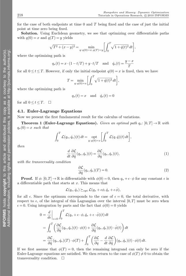
4.1. Euler-Lagrange EquationsNow we present the first fundamental result for the calculus of variations.
Theorem 1 (Euler-Lagrange Equations). Given an optimal path q∗: [0, T ]→ R withq∗(0) = x such that ∫ T
0L(q∗, q∗)(t)dt= opt
q: q(0)=x
[∫ T
0L(q, q)(t)dt
],
thend
dt
∂L∂q
(q∗, q∗)(t) =∂L∂q
(q∗, q∗)(t), (1)
with the transversality condition∂L∂q
(q∗, q∗)(T ) = 0. (2)
Proof. If φ: [0, T ]→ R is differentiable with φ(0) = 0, then q∗ + ε ·φ for any constant ε isa differentiable path that starts at x. This means that
L(q∗, q∗) opt L(q∗ + εφ, q∗ + ε φ),
for all ε. Since the optimum corresponds to the case of ε = 0, the total derivative, withrespect to ε, of the integral of this Lagrangian over the interval [0, T ] must be zero whenε= 0. Using integration by parts and the fact that φ(0) = 0 yields
0 =d
dε
∣∣∣∣ε=0
∫ T
0L(q∗ + ε ·φ, q∗ + ε · φ)(t)dt
=∫ T
0
(∂L∂q
(q∗, q∗)(t) ·φ(t)+ ∂L∂q
(q∗, q∗)(t) · φ(t))dt
=∂L∂q
(q∗, q∗)(T ) ·φ(T )+∫ T
0
(∂L∂q
− d
dt
∂L∂q
)(q∗, q∗)(t) ·φ(t)dt.
If we first assume that φ(T ) = 0, then the remaining integrand can only be zero if theEuler-Lagrange equations are satisfied. We then return to the case of φ(T ) = 0 to obtain thetransversality condition.
INFORMS
holds
copyrightto
this
article
and
distrib
uted
this
copy
asa
courtesy
tothe
author(s).
Add
ition
alinform
ation,
includ
ingrig
htsan
dpe
rmission
policies,
isav
ailableat
http://journa
ls.in
form
s.org/.
Hampshire and Massey: Dynamic OptimizationTutorials in Operations Research, c© 2010 INFORMS 219
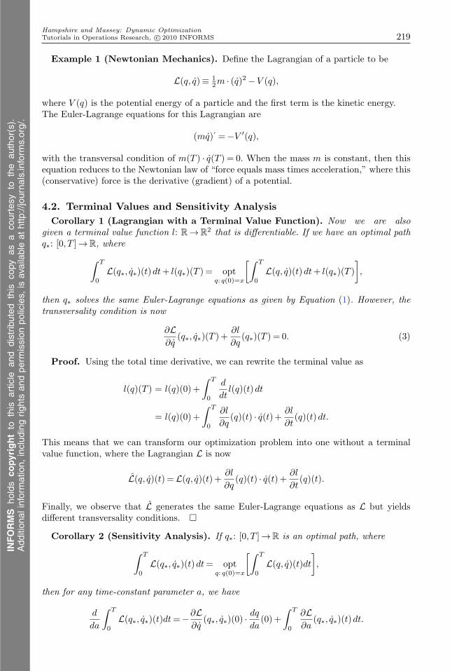
Example 1 (Newtonian Mechanics). Define the Lagrangian of a particle to be
L(q, q)≡ 12m · (q)2 −V (q),
where V (q) is the potential energy of a particle and the first term is the kinetic energy.The Euler-Lagrange equations for this Lagrangian are
(mq)· =−V ′(q),
with the transversal condition of m(T ) · q(T ) = 0. When the mass m is constant, then thisequation reduces to the Newtonian law of “force equals mass times acceleration,” where this(conservative) force is the derivative (gradient) of a potential.
4.2. Terminal Values and Sensitivity AnalysisCorollary 1 (Lagrangian with a Terminal Value Function). Now we are also
given a terminal value function l: R → R2 that is differentiable. If we have an optimal path
q∗: [0, T ]→ R, where∫ T
0L(q∗, q∗)(t)dt+ l(q∗)(T ) = opt
q: q(0)=x
[∫ T
0L(q, q)(t)dt+ l(q∗)(T )
],
then q∗ solves the same Euler-Lagrange equations as given by Equation (1). However, thetransversality condition is now
∂L∂q
(q∗, q∗)(T )+∂l
∂q(q∗)(T ) = 0. (3)
Proof. Using the total time derivative, we can rewrite the terminal value as
l(q)(T ) = l(q)(0)+∫ T
0
d
dtl(q)(t)dt
= l(q)(0)+∫ T
0
∂l
∂q(q)(t) · q(t)+ ∂l
∂t(q)(t)dt.
This means that we can transform our optimization problem into one without a terminalvalue function, where the Lagrangian L is now
L(q, q)(t) =L(q, q)(t)+ ∂l
∂q(q)(t) · q(t)+ ∂l
∂t(q)(t).
Finally, we observe that L generates the same Euler-Lagrange equations as L but yieldsdifferent transversality conditions.
Corollary 2 (Sensitivity Analysis). If q∗: [0, T ]→ R is an optimal path, where∫ T
0L(q∗, q∗)(t)dt= opt
q: q(0)=x
[∫ T
0L(q, q)(t)dt
],
then for any time-constant parameter a, we have
d
da
∫ T
0L(q∗, q∗)(t)dt=−∂L
∂q(q∗, q∗)(0) · dq
da(0)+
∫ T
0
∂L∂a
(q∗, q∗)(t)dt.
INFORMS
holds
copyrightto
this
article
and
distrib
uted
this
copy
asa
courtesy
tothe
author(s).
Add
ition
alinform
ation,
includ
ingrig
htsan
dpe
rmission
policies,
isav
ailableat
http://journa
ls.in
form
s.org/.

Hampshire and Massey: Dynamic Optimization220 Tutorials in Operations Research, c© 2010 INFORMS
Proof. Using Theorem 1 yields
d
da
∫ T
0L(q∗, q∗)(t)dt
=∫ T
0
(∂L∂q
(q∗, q∗)(t) · dqda
(t)+∂L∂q
(q∗, q∗)(t) · dqda
(t)+∂L∂a
(q∗, q∗)(t))dt
=∂L∂q
(q∗, q∗)(T ) · dqda
(T )− ∂L∂q
(q∗, q∗)(0) · dqda
(0)+∫ T
0
∂L∂a
(q∗, q∗)(t)dt
+∫ T
0
(∂L∂q
− d
dt
∂L∂q
)(q∗, q∗)(t) · dq
da(t)dt
=∫ T
0
∂L∂a
(q∗, q∗)(t)dt.
5. Constrained Lagrangian Dynamics
5.1. Multipliers and Slack VariablesWe can model the optimization of a Lagrangian subjected to equality constraints as follows.
Theorem 2 (Equality Constraints). If Φ: R2 → R is a differentiable function, then
optq: q(t)=xΦ(q, q)=0
[∫ T
0L(q, q)(t)dt
]= opt
q: q(t)=x
[∫ T
0L(q, q)(t)+ r(t) ·Φ(q, q)(t)dt
].
Moreover, the optimizing paths q∗: [0, T ]→ R and r∗: [0, T ]→ R satisfy the Euler-Lagrangeequations
d
dt
(∂L∂q
(q∗, q∗)+ r∗ · ∂Φ∂q
(q∗, q∗))(t) =
(∂L∂q
(q∗, q∗)+ r∗ · ∂Φ∂q
(q∗, q∗))(t),
with the equality constraint
Φ(q∗, q∗)(t) = 0
and the transversality condition(∂L∂q
(q∗, q∗)+ r∗ · ∂Φ∂q
(q∗, q∗))(T ) = 0.
Proof. Define the Lagrangian L, where
L(q, q, r)≡ L(q, q)+ r ·Φ(q, q),
and we are done. We now model the optimization of a Lagrangian subjected to inequality constraints.
Theorem 3 (Inequality Constraints). If Ψ: R2 → R is a differentiable mapping, then
optq: q(t)=xΨ(q, q)≥0
[∫ T
0L(q, q)(t)dt
]= opt
q: q(t)=x
[∫ T
0L(q, q)(t)+ r(t) · (Ψ(q, q)(t)−σ(t)2)dt
].
INFORMS
holds
copyrightto
this
article
and
distrib
uted
this
copy
asa
courtesy
tothe
author(s).
Add
ition
alinform
ation,
includ
ingrig
htsan
dpe
rmission
policies,
isav
ailableat
http://journa
ls.in
form
s.org/.

Hampshire and Massey: Dynamic OptimizationTutorials in Operations Research, c© 2010 INFORMS 221
Moreover, the optimizing paths q∗: [0, T ]→ R and r∗: [0, T ]→ R satisfy the Euler-Lagrangeequations
d
dt
(∂L∂q
(q∗, q∗)+ r∗ · ∂Ψ∂q
(q∗, q∗))(t) =
(∂L∂q
(q∗, q∗)+ r∗ · ∂Ψ∂q
(q∗, q∗))(t), (4)
with the inequality constraint
Φ(q∗, q∗)(t) = σ∗(t)2 ≥ 0,
the transversality condition(∂L∂q
(q∗, q∗)+ r∗ · ∂Ψ∂q
(q∗, q∗))(T ) = 0,
and the complementarity condition
r∗(t) ·σ∗(t) = 0.
Proof. Define the Lagrangian L, where
L(q, q, r, σ)≡ L(q, q)+ r · (Ψ(q, q)−σ2).
The Euler-Lagrange equations due to q give us
d
dt
∂L∂q
(q∗, q∗, r∗, σ∗) =∂L∂q∗
(q∗, q∗, r∗, σ∗).
This simplifies to (4).The Euler-Lagrange equations due to r give us
∂L∂r
(q∗, q∗, r∗, σ∗) = 0 ⇐⇒ Ψ(q∗, q∗) = σ2∗.
Finally, the Euler-Lagrange equations due to σ give us
∂L∂σ
(q∗, q∗, r∗, σ∗) = 0 ⇐⇒ r∗ ·σ∗ = 0,
and we are done.
5.2. Isoperimetric Constraints and DualityFinally, we model the optimization of a Lagrangian subjected to isoperimetric constraints.
Theorem 4 (Isoperimetric Constraints). If Θ: R2 → R is a differentiable mapping,
then
optq: q(t)=x
∫ T0 Θ(q, q)(t)dt=0
[∫ T
0L(q, q)(t)dt
]= opt
q: q(t)=xb: b(0)=b(T )=0,
[∫ T
0L(q, q)(t)+a(t) · (b(t)−Θ(q, q)(t))dt
].
This optimization problem simplifies to
optq: q(t)=x
∫ T0 Θ(q, q)(t)dt=0
[∫ T
0L(q, q)(t)dt
]= opt
q: q(t)=x
[∫ T
0(L − a ·Θ)(q, q)(t)dt
].
INFORMS
holds
copyrightto
this
article
and
distrib
uted
this
copy
asa
courtesy
tothe
author(s).
Add
ition
alinform
ation,
includ
ingrig
htsan
dpe
rmission
policies,
isav
ailableat
http://journa
ls.in
form
s.org/.

Hampshire and Massey: Dynamic Optimization222 Tutorials in Operations Research, c© 2010 INFORMS
Moreover, the optimal path q∗: [0, T ]→ R satisfies the Euler-Lagrange equations
d
dt
(∂L∂q
− a · ∂Θ∂q
)(q∗, q∗)(t) =
(∂L∂q
− a · ∂Θ∂q
)(q∗, q∗)(t), (5)
with the transversality condition of(∂L∂q
− a · ∂Θ∂q
)(q∗, q∗)(T ) = 0, (6)
and a is a constant that satisfies the isoperimetric condition of∫ T
0Θ(q∗, q∗)(t)dt= 0. (7)
Proof. Define the Lagrangian L, where
L(a, b, q, q)≡ L(q, q)+ a · (b−Θ(q, q)),
where we add the boundary conditions of b(0) = b(T ) = 0.The Euler-Lagrange equations due to q give us
d
dt
∂L∂q
(a∗, b∗, q∗, q∗) =∂L∂q∗
(a∗, b∗, q∗, q∗).
This simplifies to (5). The transversality condition of (6) is similarly derived.The Euler-Lagrange equations due to a give us
∂L∂a
(a∗, b∗, q∗, q∗) = 0 ⇐⇒ b∗ =Θ(q∗, q∗).
Integrating the latter equation over the interval (0, T ], combined with the conditions ofb(0) = b(T ) = 0, gives us (7).Finally, the Euler-Lagrange equations due to b give us
d
dt
∂L∂b
(a∗, b∗, q∗, q∗) = 0 ⇐⇒ a∗ = 0.
This makes a∗ a constant over time, and we are done. Problem 2 (Maximizing Area Constrained by Perimeter). As illustrated in Fig-
ure 3, find the maximal area |Ω|, for a simply connected region Ω in R2, bounded by a fixed
perimeter |∂Ω| of the boundary ∂Ω.Solution. Let (x, y): (0, T ] → ∂Ω be a one-to-one differentiable mapping and (x, y):
[0, T ] → ∂Ω a differentiable mapping. Moreover, we assume that x(0) = x(T ), x′(0+) =x′(T−), and y has the same properties.We can compute the perimeter of ∂Ω by using this parameterization of the boundary
for Ω and get
|∂Ω|=∫ T
0
√x(t)2+ y(t)2 dt. (8)
We can also use the parameterization of the boundary curve ∂Ω to express the area of Ω asa line intergral. This yields
|Ω|= 12
∫ T
0(x(t) y(t)− y(t) x(t))dt,
INFORMS
holds
copyrightto
this
article
and
distrib
uted
this
copy
asa
courtesy
tothe
author(s).
Add
ition
alinform
ation,
includ
ingrig
htsan
dpe
rmission
policies,
isav
ailableat
http://journa
ls.in
form
s.org/.

Hampshire and Massey: Dynamic OptimizationTutorials in Operations Research, c© 2010 INFORMS 223
Figure 3. Finding the maximum area given a fixed perimeter for the boundary.
(x(0), y(0)) = (x(T ), y(T ))
(x(t ), y(t ))
T
0|Ω| = ∫ x(t )2 + y(t )2 dt
|Ω| = ∫∫ dx∧dyΩ
• •
since by Green’s theorem we have
|Ω|=∫∫
Ωdx∧ dy= 1
2
∫∂Ω
xdy− y dx.
Now we have an optimization problem with an isoperimetric constraint. Our Lagrangian is
L(a, b, x, x, y, y) = 12 (x y− y x)+ a · (b−
√x 2+ y 2).
The Euler-Lagrange equations for x are
d
dt
∂L∂x
=∂L∂x
⇐⇒ d
dt
(−12y(t)− a · x(t)√
x(t)2+ y(t)2
)=
12y(t). (9)
Similarly for y we have
d
dt
∂L∂y
=∂L∂y
⇐⇒ d
dt
(12x(t)− a · y(t)√
x(t)2+ y(t)2
)=−1
2x(t). (10)
For the state variable b, we have
d
dt
∂L∂b
=∂L∂b
= 0 ⇐⇒ a(t) = 0
for all 0≤ t≤ T . This means that a is a constant. Finally, for its dual variable b we have
0 =d
dt
∂L∂a
=∂L∂a
⇐⇒ b(t) =√x(t)2+ y(t)2.
Coupled with the initial and terminal conditions of b(0) = 0 and b(T ) = |∂Ω|, we thenhave (8).
Simplifying (9) and (10) yields
d
dt
(−y(t)− a · x(t)√
x(t)2+ y(t)2
)= 0 and
d
dt
(x(t)− a · y(t)√
x(t)2+ y(t)2
)= 0.
This means that there exists two constants ξ and η such that
y(t)− η=a · x(t)√
x(t)2+ y(t)2and x(t)− ξ =
a · y(t)√x(t)2+ y(t)2
.
From this it follows that x(t) and y(t) solve the algebraic equation
(x(t)− ξ)2+(y(t)− η)2 = a2.
This means that Ω is a circle of radius a. The last step is to select a such that |∂Ω|= 2πa.
INFORMS
holds
copyrightto
this
article
and
distrib
uted
this
copy
asa
courtesy
tothe
author(s).
Add
ition
alinform
ation,
includ
ingrig
htsan
dpe
rmission
policies,
isav
ailableat
http://journa
ls.in
form
s.org/.

Hampshire and Massey: Dynamic Optimization224 Tutorials in Operations Research, c© 2010 INFORMS
We can apply these same arguments to solve a dual problem.Problem 3 (Minimizing Perimeter Constrained by Area). Find the minimal per-
imeter |∂Ω|, for the boundary ∂Ω of a simply connected region Ω in R2, given a fixed
area |Ω|.Suppose that we start with a given area value. Solving Problem 3 yields the minimal
perimeter for this area. Conversely, if we assume this minimizing perimeter value, then themaximal area from the solution to Problem 2 is precisely the originally given area value.This is the continuous state version of the duality principle for linear programming. Here,the concepts of area and perimeter implicitly give us quantities that are always positive.Below, we give a more generalized notion of this duality.
Theorem 5. Suppose that we have Lagrangians L and M such that:
(1) For all constants x, there exists an optimal path qx∗ (t) | t≥ 0 such that
f(x)≡∫ T
0(L −x · M)(qx∗ , q
x∗)(t)dt=max
q
∫ T
0(L −x · M)(q, q)(t)dt.
(2) The function f is convex with f(0)> 0, f ′(0)< 0, and
minx>0
f(x) = 0.
It follows that
maxq:
∫ T0 M(q, q)(t)dt=0
∫ T
0L(q, q)(t)dt= min
q:∫ T0 L(q, q)(t)dt=0
∫ T
0M(q, q)(t)dt= 0
and
minx>0
(maxq
∫ T
0(L −x · M)(q, q)(t)dt
)=max
x>0
(minq
∫ T
0(M −x · L)(q, q)(t)dt
)= 0.
Proof. Given the sensitivity results, we have
f ′(x) =−∫ T
0M(qx∗ , q
x∗)(t)dt= 0.
The conditions of f(0)> 0 and f ′(0)< 0 translate into∫ T
0L(q0∗, q 0∗)(t)dt=max
q
∫ T
0L(q, q)(t)dt > 0
and ∫ T
0M(q0∗, q
0∗)(t)dt > 0.
Starting from zero, f is a decreasing function as long as f ′(x)> 0. Since there exists anx∗ > 0 with f(x∗) = 0, we then have f ′(x∗) = 0 and so
maxq:
∫ T0 M(q, q)(t)dt=0
∫ T
0L(q, q)(t)dt=min
x>0f(x) = 0.
Now qx∗ (t) | t≥ 0 solves the Euler-Lagrange equations for L −x · M. Since
M − 1x∗
· L=− 1x
· (L −x · M),
it follows that qx∗ (t) | t≥ 0 also solves the Euler-Lagrange equations for M − 1/x∗ · L.
INFORMS
holds
copyrightto
this
article
and
distrib
uted
this
copy
asa
courtesy
tothe
author(s).
Add
ition
alinform
ation,
includ
ingrig
htsan
dpe
rmission
policies,
isav
ailableat
http://journa
ls.in
form
s.org/.

Hampshire and Massey: Dynamic OptimizationTutorials in Operations Research, c© 2010 INFORMS 225
Now we define the function g(x), where
g(x)≡minq
∫ T
0(L −x · M)(q, q)(t)dt.
Based on our assumptions, there exists an x∗ such that f(x∗) = f ′(x∗) = 0. For all positive x,we then have
g(x) =−x · f(1x
).
Through various operations such as differentiating and multiplying by x, we obtain
g′(x) =−f(1x
)− 1x
· f(1x
)and g′′(x) =−f ′′
(1x
).
It now follows that g is a negative, concave function with g(1/x∗) = g′(1/x∗) = 0; henceg attains its maximum at 1/x∗ and
g(1/x∗) =maxx>0
g(x) = 0.
5.3. Conserved QuantitiesWe conclude this section by showing how to construct quantities that are conserved along theoptimal Lagrangian path. The following result is adapted from Sato and Ramachandran [44].
Theorem 6. Let θ parameterize a differentiable transformation from (q(t), t) to(qθ(tθ), tθ), where
qθ(tθ) = qθ(q(t), q(t), t) and tθ = tθ(q(t), q(t), t),
with q(t) = q0(t0) and t= t0. If we have
d
dtG(q(t), t) = d
dθ
(L(qθ(tθ), qθ(tθ), tθ) · d
dttθ
)∣∣∣∣θ=0
, (11)
then the deterministic process
G(q)− ∂L∂q
(q, q) · q(q, q)−(
L(q, q)− ∂L∂q
(q, q) · q)
· t(q, q)
is a conserved quantity along the optimal path, where
q(q, q)≡ d
dθqθ(q, q)
∣∣∣∣θ=0
and t(q, q)≡ d
dθtθ(q, q)
∣∣∣∣θ=0
.
Proof. Observe that
qθ(tθ) =d
dtqθ(q(t), q(t), t)
/d
dttθ(q(t), q(t), t) = qθ(q(t), q(t), t)
/tθ(q(t), q(t), t).
This means that we can rewrite (11) as
G(q) = d
dθL(qθ(q, q), qθ(q, q)
/tθ(q, q), tθ(q, q)) · tθ(q, q)|θ=0.
Along the optimal path, the Euler-Lagrange equations hold, so we have
d
dt
∂L∂q
(q∗(t), q∗(t), t) =∂L∂q
(q∗(t), q∗(t), t).
INFORMS
holds
copyrightto
this
article
and
distrib
uted
this
copy
asa
courtesy
tothe
author(s).
Add
ition
alinform
ation,
includ
ingrig
htsan
dpe
rmission
policies,
isav
ailableat
http://journa
ls.in
form
s.org/.

Hampshire and Massey: Dynamic Optimization226 Tutorials in Operations Research, c© 2010 INFORMS
The rest follows from the computation below:
d
dθ
(L(qθ(q∗, q∗), qθ(q∗, q∗)/tθ(q∗, q∗), tθ(q∗, q∗)) · tθ(q∗, q∗))∣∣θ=0
=∂L∂q
(q∗, q∗) · q(q∗, q∗)+∂L∂q
(q∗, q∗) · ( ˙q(q∗, q∗)− q∗ · ˙t(q∗, q∗))
+∂L∂t
(q∗, q∗) · t(q∗, q∗)+L(q∗, q∗) · ˙t(q∗, q∗)
=d
dt
(∂L∂q
(q∗, q∗))
· q(q∗, q∗)+∂L∂q
(q∗, q∗) · ˙q(q∗, q∗)− ∂L∂q
(q∗, q∗) · q∗ · ˙t(q∗, q∗)
+d
dt
(L(q∗, q∗)− ∂L
∂q(q∗, q∗) · q∗
)· t(q∗, q∗)+L(q∗, q∗) · ˙t(q∗, q∗)
=d
dt
(∂L∂q
(q∗, q∗))
· q(q∗, q∗)+∂L∂q
(q∗, q∗) · ˙q(q∗, q∗)
+d
dt
(L(q∗, q∗)− ∂L
∂q(q∗, q∗) · q∗
)· t(q∗, q∗)+
(L(q∗, q∗)− ∂L
∂q(q∗, q∗) · q∗
)· ˙t(q∗, q∗)
=d
dt
(∂L∂q
(q∗, q∗) · q(q∗, q∗)+(
L(q∗, q∗)− ∂L∂q
(q∗, q∗) · q∗
)· t(q∗, q∗)
).
6. The HamiltonianFrom the perspective of classical mechanics, the Lagrangian through the Euler-Lagrangeequations successfully captured the laws of Newtonian physics. However, quantities like itand its time integral called “action” had no physical interpretation. They were merely math-ematical formalisms that worked. One could attribute this to the fact that philosophicallyclassical physics was not thought of in terms of quantities that are optimized. This is incontrast to the operations research and economic views of the Lagrangian. Here, we caninterpret the Lagrangian as a “value rate” since operations researchers and economists nat-urally maximize quantities like “profit” or “revenue” and minimize quantities like “loss” or“cost.”We formally define the Hamiltonian in terms of the Lagrangian to be
H(p, q, t)≡ optv∈R
(p · v− L(q, v, t)). (12)
The optimization method that yields the Hamiltonian is called the Legendre transform.In the next section we study its special properties. Instead of using the optimal pathsand velocities of q∗ and q∗, we keep the former but replace the latter with a generalizedmomentum variable p∗. This allows us to replace the Euler-Lagrange equations for positionand velocity with the equivalent set of Hamilton’s equations for position and momentum.Unlike the Euler-Lagrange equations, Hamilton’s equations are always dynamical systems.These are evolution equations that lend themselves to computationally simple numericalsolutions. Finally, the Hamiltonian perspective helps us identify conserved quantities. Inaddition to terms like energy and momentum, there may be other conservation principlesat work for a given Hamiltonian system.
6.1. Legendre TransformsFirst, for some function l: R → R, we define the Legendre transform (when it exists) to bethe function h: R → R, such that
h(p)≡ optv∈R
(p · v− l(v)).
INFORMS
holds
copyrightto
this
article
and
distrib
uted
this
copy
asa
courtesy
tothe
author(s).
Add
ition
alinform
ation,
includ
ingrig
htsan
dpe
rmission
policies,
isav
ailableat
http://journa
ls.in
form
s.org/.
Hampshire and Massey: Dynamic OptimizationTutorials in Operations Research, c© 2010 INFORMS 227
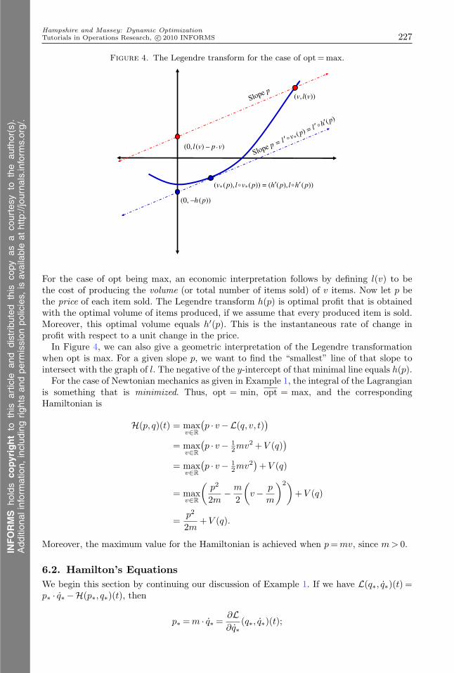
Figure 4. The Legendre transform for the case of opt =max.
Slope p
Slope p = l ′ °v*(p) = l ′ °h′(p)
(v, l(v))
(0, l (v) – p .v)
(0, –h (p))
(v*(p), l°v*(p)) = (h′(p), l°h′ (p))
For the case of opt being max, an economic interpretation follows by defining l(v) to bethe cost of producing the volume (or total number of items sold) of v items. Now let p bethe price of each item sold. The Legendre transform h(p) is optimal profit that is obtainedwith the optimal volume of items produced, if we assume that every produced item is sold.Moreover, this optimal volume equals h′(p). This is the instantaneous rate of change inprofit with respect to a unit change in the price.In Figure 4, we can also give a geometric interpretation of the Legendre transformation
when opt is max. For a given slope p, we want to find the “smallest” line of that slope tointersect with the graph of l. The negative of the y-intercept of that minimal line equals h(p).For the case of Newtonian mechanics as given in Example 1, the integral of the Lagrangian
is something that is minimized. Thus, opt = min, opt = max, and the correspondingHamiltonian is
H(p, q)(t) = maxv∈R
(p · v− L(q, v, t))
= maxv∈R
(p · v− 1
2mv2+V (q))
= maxv∈R
(p · v− 1
2mv2)+V (q)
= maxv∈R
(p2
2m− m
2
(v− p
m
)2)+V (q)
=p2
2m+V (q).
Moreover, the maximum value for the Hamiltonian is achieved when p=mv, since m> 0.
6.2. Hamilton’s EquationsWe begin this section by continuing our discussion of Example 1. If we have L(q∗, q∗)(t) =p∗ · q∗ − H(p∗, q∗)(t), then
p∗ =m · q∗ =∂L∂q∗
(q∗, q∗)(t);
INFORMS
holds
copyrightto
this
article
and
distrib
uted
this
copy
asa
courtesy
tothe
author(s).
Add
ition
alinform
ation,
includ
ingrig
htsan
dpe
rmission
policies,
isav
ailableat
http://journa
ls.in
form
s.org/.

Hampshire and Massey: Dynamic Optimization228 Tutorials in Operations Research, c© 2010 INFORMS
hence∂H∂p
(p∗, q∗)(t) =p∗m
= q∗ and∂H∂q
(p∗, q∗)(t) = V ′(q∗) =−p∗.
Finally, observe that if the mass m is constant, then
d
dtH(p∗, q∗)(t) =
p∗m
· p∗ +V ′(q∗) · q∗ = q∗ · p∗ − p∗ · q∗ = 0.
Thus along the optimum path, H(p∗, q∗)(t) is a constant over time.We now summarize these results in a larger framework.
Theorem 7 (Hamilton’s Equations). If we have
H(p∗, q∗)(t) = p∗(t) · q∗(t)− L(q∗, q∗)(t), (13)
then
p∗(t) =∂L∂q
(q∗, q∗)(t). (14)
Moreover, we have
p∗(t) =−∂H∂q
(p∗, q∗)(t) and q∗(t) =∂H∂p
(p∗, q∗)(t). (15)
Proof. Our definition of the Hamiltonian means that we have some v∗(p, q, t) such that
H(p, q, t) = p · v∗(p, q, t)− L(q, v∗(p, q, t), t). (16)
Now we make the substitutions
p= p∗(t), q= q∗(t), and v∗(p∗, q∗)(t) = q∗(t). (17)
The Equation (14) follows from (13), since
0 =∂
∂v
∣∣∣∣v∗(p, q, t)
(p · v− L(q, v, t)) implies that p=∂L∂q
(q, v∗(p, q, t), t).
The computation of the partial derivatives of the Hamiltonian with respect to p and q in(16) simplifies considerably due to the envelope lemma (see Lemma 1). This result allowsus to ignore the dependence of v(p, q) on p and q and state that
∂H∂p
(p, q, t) = v∗(p, q, t) and∂H∂q
(p, q, t) =−∂L∂q
(q, v∗(p, q, t), t).
Now Hamilton’s equations (15) follow from applying the substitutions of (17), (14), and theEuler-Lagrange equations (1).
6.3. Computing Hamiltonian FlowsGiven a Lagrangian L and an optimal position coordinate q∗ yields a Hamiltonian H andwhat we define to be an optimal momentum coordinate p∗ given by (14). The coordinatepair of p∗ and q∗ describes a point in phase space. The evolution of these coordinates overtime (p∗(t), q∗(t)) |0≤ t≤ T is called a Hamiltonian flow. We now state an algorithm forcomputing this flow (see Figure 5). Initially, we assume that
q0(t) = q(0)
for all 0 ≤ t ≤ T . Now we iterate through time loops that start at time T , go back to thepast of time 0, and then go back to the future of time T . Recursively, the nth time loop,
INFORMS
holds
copyrightto
this
article
and
distrib
uted
this
copy
asa
courtesy
tothe
author(s).
Add
ition
alinform
ation,
includ
ingrig
htsan
dpe
rmission
policies,
isav
ailableat
http://journa
ls.in
form
s.org/.

Hampshire and Massey: Dynamic OptimizationTutorials in Operations Research, c© 2010 INFORMS 229
Figure 5. A flow chart diagram for computing Hamilton’s equations.
n = 1
pn ≈ p*
qn ≈ q*
n ≤ iteration number?
Solve 0 ⇐ t ⇐ T
Solve 0 ⇒ t ⇒ T
with pn(T ) = 0
with qn(0) = q (0)
n++
Set q0(t ) = q (0)for all 0 ≤ t ≤ T
pn(t ) = – (pn(t ),qn–1(t ), t)
q
qn(t ) = – (pn(t ),qn(t ), t)
p
•
•
where n≥ 1, is
(1) Given qn−1(t) |0≤ t≤ T , solve for the dynamical system
pn(t) =−∂H∂q
(pn, qn−1)(t)
backward in time for 0≤ t≤ T , starting with the terminal condition pn(T ) = 0.(2) Given pn(t) |0≤ t≤ T , solve for the dynamical system
qn(t) =∂H∂p
(pn, qn)(t)
forward in time for 0≤ t≤ T , starting with the initial condition qn(0) = q(0).
6.4. Poisson Brackets and Conservation PrinciplesCorollary 3 (Conservation of Momentum). Along the Hamiltonian flow, we have
∂L∂q
(p∗, q∗)(t) = 0 if and only if∂H∂q
(p∗, q∗)(t) = 0.
Moreover, both statements are equivalent to p∗(t) = 0.
Proof. Using the Euler-Lagrange equations (1) and Hamilton’s equations (15) yields
p∗(t) =∂L∂q
(p∗, q∗)(t) =−∂H∂q
(p∗, q∗)(t).
Corollary 4 (Conservation of Energy). Along the Hamiltonian flow, whenever wehave
∂H∂t
(p∗, q∗)(t) = 0,
it follows that
d
dtH(p∗, q∗)(t) = 0.
INFORMS
holds
copyrightto
this
article
and
distrib
uted
this
copy
asa
courtesy
tothe
author(s).
Add
ition
alinform
ation,
includ
ingrig
htsan
dpe
rmission
policies,
isav
ailableat
http://journa
ls.in
form
s.org/.

Hampshire and Massey: Dynamic Optimization230 Tutorials in Operations Research, c© 2010 INFORMS
Proof. Using Theorem 7 yields
d
dtH(p∗, q∗)(t) =
∂H∂p
(p∗, q∗)(t) · p∗(t)+∂H∂q
(p∗, q∗)(t) · q∗(t)+∂H∂t
(p∗, q∗)(t)
= q∗(t) · p∗(t)− p∗(t) · q∗(t)
= 0.
These two results are a part of a larger conservation principle. We define an observable forthe Hamiltonian flow to be any differentiable mapping Φ: R
2 × [0, T ]→ R. Now we describethe dynamics of Φ(p∗, q∗).
Corollary 5 (Poisson Brackets). Given a Hamiltonian H, let p∗ and q∗ be optimalpaths that solve Hamilton’s equations (15). If Φ is an observable, then
d
dtΦ(p∗, q∗)(t) =
(Φ,H+ ∂Φ
∂t
)(p∗, q∗)(t),
where ·, · is the Poisson bracket that is defined by the formula
Φ,Ψ(p, q, t)≡(∂Φ∂q
· ∂Ψ∂p
− ∂Ψ∂q
· ∂Φ∂p
)(p, q, t), (18)
where Ψ is another observable.
Proof. Applying the chain rule for the total differential with respect to t yields
d
dtΦ(p∗, q∗)(t) =
∂Φ∂p
(p∗, q∗)(t) · p∗(t)+∂Φ∂q
(p∗, q∗)(t) · q∗(t)+∂Φ∂t
(p∗, q∗)(t)
=(
−∂Φ∂p
· ∂H∂q
+∂Φ∂q
· ∂H∂p
+∂Φ∂t
)(p∗, q∗)(t).
Now we apply (18) to (19), and we are done. The Poisson bracket also has various algebraic properties. First, it is antisymmetric; i.e.,
for all observables Φ and Ψ, we have
Φ,Ψ=−Ψ,Φ.Moreover, it is also a bilinear operation, with
Φ+Ψ,H= Φ,H+ Ψ,Hand
a ·Φ,H= a · Φ,H.Finally, the Poisson bracket satisfies the Jacobi identity or
Φ,Ψ,H= Φ,Ψ,H − Ψ,Φ,H.The Poisson bracket has the following geometric interpretation for two observables that
are not time dependent or Φ and Ψ where
∂Φ∂t
=∂Ψ∂t
= 0.
In Figure 6, we fix t and view Φ and Ψ as scalar fields over the “phase space” given by themomentum and position coordinates of p and q, respectively. The dotted curve represents acontour for Φ or the set of phase-space coordinates where it equals some constant a. The solidcurve plays a similar role as the contour for Ψ equalling a constant b. The gradient of Φ is
INFORMS
holds
copyrightto
this
article
and
distrib
uted
this
copy
asa
courtesy
tothe
author(s).
Add
ition
alinform
ation,
includ
ingrig
htsan
dpe
rmission
policies,
isav
ailableat
http://journa
ls.in
form
s.org/.

Hampshire and Massey: Dynamic OptimizationTutorials in Operations Research, c© 2010 INFORMS 231
Figure 6. A geometric interpretation of the Poisson bracket.
Φ ≡ a Φ,Ψ(p,q)
∇Ψ(p,q)
∇Φ (p,q)
(p,q)Ψ ≡ b
the direction of greatest change for its scalar field. It is always orthogonal to the tangent linefor the contour curve at that point (p, q). Locally, this means that the gradient is orthogonalto the direction that “conserves Φ.” The gradient for Ψ has a similar interpretation. ThePoisson bracket is then the area (up to a sign for orientation) of the parallelogram formedby the two gradients at a given point (p, q) in phase space. This area is zero if and only if thetwo gradients are colinear or they “point in the same direction” (up to a sign). When thePoisson bracket is zero along the contour of one of them, then the same curve is a contourfor the other and it is possible to move through phase space in a direction that conservesboth observables Φ and Ψ. For more on the algebraic structure of Hamiltonian dynamics,see Marsden and Ratiu [34].We define an observable Φ to be a conserved quantity over the interval [0, T ] if
d
dtΦ(p∗, q∗)(t) = 0.
Now we can characterize the underlying structure of conserved quantities.
Corollary 6. An observable Φ is a conserved quantity over the interval [0, T ] whenever(∂Φ∂t
+ Φ,H)(p∗, q∗)(t) = 0
for all 0≤ t≤ T . Moreover, the set of conserved quantities form a vector space that is alsoclosed with respect to the Poisson bracket operation.
Proof. Given two conserved quantities Φ and Ψ, we have
∂
∂tΦ,Ψ =
∂Φ∂t
,Ψ+Φ,
∂Ψ∂t
= −Φ,H,Ψ − Φ,Ψ,H= Ψ,Φ,H − Φ,Ψ,H= Ψ,Φ,H= −Φ,Ψ,H.
The third step follows from the Jacobi identity.
INFORMS
holds
copyrightto
this
article
and
distrib
uted
this
copy
asa
courtesy
tothe
author(s).
Add
ition
alinform
ation,
includ
ingrig
htsan
dpe
rmission
policies,
isav
ailableat
http://journa
ls.in
form
s.org/.

Hampshire and Massey: Dynamic Optimization232 Tutorials in Operations Research, c© 2010 INFORMS
We have now shown that the family of conserved quantities form a Lie algebra withrespect to addition and the Poisson bracket operation as our anticommutative, nonasso-ciative multiplication. If we are given two or more conserved quantities, we can then uselinear combinations of them and the Poisson bracket to generate the associated Lie algebraof additional conserved quantities.For operations research problems, the Hamiltonian formulation is useful from a computa-
tional perspective. It is easier to numerically solve differential equations that are dynamicalsystems than some of the Euler-Lagrange equations derived from Lagrangian mechanics.This simplicity is somewhat compromised by the mixed boundary values of an initial valuefor q paired with a terminal value of p(T ) = 0. However, the dynamical system structuresuggests an iterative method for the solution. The nature of the method suggests evolvingforwards in time with q but backward in time with p. The Hamiltonian formulation alsoprovides us with a Lie algebra calculus to derive conserved quantities.
6.5. Envelope LemmaWe conclude this section with a precise statement and proof of the envelope lemma.
Lemma 1 (Envelope Lemma). Let O ⊆ R2 be open and f : O → R be differentiable. If
for all x, there exists some φ(x) such that
f(x,φ(x)) = opt−∞<y<∞
f(x, y), (19)
then
d
dxf(x,φ(x)) =
∂f
∂x(x,φ(x)).
Proof. Since f is differentiable, then by (19) we have
∂f
∂y(x,φ(x)) = 0.
The rest follows by taking the total derivative of f(x,φ(x)) with respect to x and using thechain rule.
7. The Bellman Value FunctionThe Bellman value function can be defined in terms of the Lagrangian as follows:
V(x, t)≡ optq: q(t)=x
[∫ T
t
L(q, q)(s)ds].
We show in this section how the Bellman value function yields a unifying framework forinterpreting Lagrangians and Hamiltonians from an operations research perspective.
7.1. Bellman Principle of OptimalityRather than derive the Euler-Lagrange equations, we can find the optimal path by using theequivalent fundamental principle of optimality due to Bellman (see Pedregal [40]), where
V(q∗)(t) = optq: q(t)=x
[∫ τ
t
L(q, q)(s)ds+V(q)(τ)], (20)
for all intermediate times τ where t≤ τ ≤ T .
INFORMS
holds
copyrightto
this
article
and
distrib
uted
this
copy
asa
courtesy
tothe
author(s).
Add
ition
alinform
ation,
includ
ingrig
htsan
dpe
rmission
policies,
isav
ailableat
http://journa
ls.in
form
s.org/.

Hampshire and Massey: Dynamic OptimizationTutorials in Operations Research, c© 2010 INFORMS 233
Figure 7. Bellman principle of optimality.
A
BC
D
Problem 4 (Shortest Path Around an Obstacle). Consider two points in theEuclidean plane. They are denoted by A and D, as illustrated in Figure 7. The shortest pathbetween them that is constrained to stay outside the disk is given by the unions of the linesAB and CD with is shortest of the circular arcs BC.
Solution. A simple way to show that this is the minimum path is by applying theBellman principle. The subset of the path that connects C and D must be a straight linesince that is the shortest distance in general and it is a line segment that is outside thedisk. A similar argument can be made for why the subset of the path that connects A andB is also a straight line. Finally, we observe that a circle is defined to have the maximumarea for a given perimeter. This means that the smaller of the two circular arcs connectingB and C is the minimum distance between the two points when the path is constrained tostay outside the disk.
7.2. Hamilton-Jacobi-Bellman EquationThe Bellman value function is defined in terms of the Lagrangian. In this section, weshow how along the optimal path we can use the Bellman value function to construct theHamiltonian.
Theorem 8 (Hamilton-Jacobi-Bellman Equation). If the Bellman value function istwice differentiable, then we have
∂V∂t
(x, t) =H(
−∂V∂q
(x, t), x, t). (21)
Moreover,
p∗(t) =−∂V∂q
(q∗)(t) and H(p∗, q∗)(t) =∂V∂t
(q∗)(t). (22)
Proof. Using the Bellman principle of optimality (20), subtracting V(x, t), dividing byτ − t, and taking the limit as τ approaches t yields
0 = optq: q(t)=x
[∫ τ
t
L(q, q)(s)ds+V(q)(τ)− V(q)(t)]
INFORMS
holds
copyrightto
this
article
and
distrib
uted
this
copy
asa
courtesy
tothe
author(s).
Add
ition
alinform
ation,
includ
ingrig
htsan
dpe
rmission
policies,
isav
ailableat
http://journa
ls.in
form
s.org/.

Hampshire and Massey: Dynamic Optimization234 Tutorials in Operations Research, c© 2010 INFORMS
= optq: q(t)=x
[1
τ − t
∫ τ
t
L(q, q)(s)ds+ V(q)(τ)− V(q)(t)τ − t
]= opt
q: q(t)=x
[L(q, q)(t)+ d
dtV(q)(t)
]= opt
q: q(t)=x
[L(q, q)(t)+ ∂V
∂q(q)(t) · q(t)+ ∂V
∂t(q)(t)
]= opt
v∈R
[L(x, v, t)+ ∂V
∂q(x, t) · v+ ∂V
∂t(x, t)
]= opt
v∈R
[L(x, v, t)+ ∂V
∂q(x, t) · v
]+∂V∂t
(x, t).
So finally, we have
∂V∂t
(x, t) =− optv∈R
[L(x, v, t)+ ∂V
∂q(x, t) · v
]= opt
v∈R
[−∂V∂q
(x, t) · v− L(x, v, t)],
which yields (21). Finally, (22) follows from using the Bellman principle of optimality. Forevery intermediate time τ , where 0 ≤ τ ≤ T , we have an equivalent optimization problemwhere the Bellman value function is now the additional terminal value function at the newterminal time τ . Using (3) from Corollary 1 yields, on the left-hand side, the formula for thegeneralized momentum variable p∗(t). From this follows the right-hand side formula of (3)for the Hamiltonian. For operations research problems, the Bellman value function formulation is useful from
a perspective of interpreting optimality. The partial derivatives have the interpretation ofopportunity costs. The Hamilton-Jacobi-Bellman equation says that the generalized momen-tum variable is the opportunity cost density and the Hamiltonian is the opportunity costrate.
8. Optimal ControlIn this section we show how all three methods of dynamic optimizations, the Lagrangian,Hamiltonian, and Bellman value function, all contribute to solving problems in optimalcontrol.
V(x, t)≡ optq: q(t)=x, r∈Kq=l(q(t), r(t), t)
[∫ T
t
L(q, r)(s)ds],
where K is some compact subset of R. Moreover, L: R ×K × [0, T ] → R is differentiablein the first and last arguments but optimally semi-continuous (i.e., upper semi-continuouswhen opt is max and lower semi-continuous otherwise) with respect to the middle argument.We define l: R × K × [0, T ] → R in a similar manner except that we assume that it is acontinuous function of the middle argument.Since this optimization problem only involves the state variable r and not its time deriva-
tive, we refer to r as a control variable. We want to extend our methods for dynamicoptimization to cover the cases where the control variable range is confined to a compact setand the Lagrangian may not be a differentiable function in the control variable argument.
8.1. Pontryagin PrincipleSuppose that we are given the control variable r. Our problem is then one of constrainedoptimization. The Lagrangian L for this problem is
L(p, q, q, r, t) = L(q, r, t)+ p · (q− l(q, r, t)).
INFORMS
holds
copyrightto
this
article
and
distrib
uted
this
copy
asa
courtesy
tothe
author(s).
Add
ition
alinform
ation,
includ
ingrig
htsan
dpe
rmission
policies,
isav
ailableat
http://journa
ls.in
form
s.org/.

Hampshire and Massey: Dynamic OptimizationTutorials in Operations Research, c© 2010 INFORMS 235
Since this Lagrangian is a linear function of q, its Legendre transform is well defined exactlyat p, which yields
H(p, q, r, t) = p · l(q, r, t)−L(q, r, t).In this section we show that V(x, t) is a Bellman value function by deriving its
Hamiltonian. We achieve this by constructing the position and momentum variables thatsolve Hamilton’s equations.
Theorem 9 (Pontryagin Principle). For this optimal control problem, we have
H(p∗, q∗, r∗)(t) = optρ∈K
H(p∗(t), q∗(t), ρ, t),
where
p∗(t) =−∂H∂q
(p∗, q∗, r∗)(t) and q∗(t) =∂H∂p
(p∗, q∗, r∗)(t)
for all 0≤ t≤ T with p∗(T ) = 0, and q∗(0) is given.
Proof. Given a optimal path q∗: [0, T ] → R and an optimal control r∗: [0, T ] → K, weneed only show that
p∗(t) =−∂V∂q
(q∗)(t).
Since we have
V(q∗)(t)≡∫ T
t
L(q∗, r∗)(s)ds,
it follows that
∂V∂t
(q∗)(t) =−∂V∂q
(q∗)(t) · l(q∗, r∗)(t)−L(q∗, r∗)(t).
Equating this with (23) of Lemma 2, when x= q∗(t), yields
−∂V∂q
(q∗)(t) · l(q∗, r∗)(t)−L(q∗, r∗)(t) = optρ∈K
[−∂V∂q
(q∗)(t) · l(q∗(t), ρ, t)−L(q∗(t), ρ, t)].
Finally, we use (25) with x= q∗(t), ρ∗(x, t) = r∗(t) and the chain rule to show that
d
dt
(−∂V∂q
(q∗)(t))=−
(−∂V∂q
(q∗)(t) · ∂l∂q
(q∗, r∗)(t)− ∂L∂q
(q∗, r∗)(t)).
Lemma 2. We have for all x and t
∂V∂t
(x, t) = optρ∈K
H(
−∂V∂q
(x, t), x, ρ, t), (23)
where there exists some ρ∗(x, t)∈K such that
∂V∂t
(x, t) =H(
−∂V∂q
(x, t), x, ρ∗(x, t), t)
(24)
and
∂2V∂t∂q
(x, t)+∂2V∂q2
(x, t) · l(x,ρ∗(x, t), t) =∂H∂q
(−∂V∂q
(x, t), x, ρ∗(x, t), t). (25)
INFORMS
holds
copyrightto
this
article
and
distrib
uted
this
copy
asa
courtesy
tothe
author(s).
Add
ition
alinform
ation,
includ
ingrig
htsan
dpe
rmission
policies,
isav
ailableat
http://journa
ls.in
form
s.org/.
Hampshire and Massey: Dynamic Optimization236 Tutorials in Operations Research, c© 2010 INFORMS
Proof. Using a similar argument to the one we use for the Bellman value function, wehave
0 = optq: q(t)=x
q=l(q, r)(t)
[∫ τ
t
L(q, r)(s)ds+ V(q)(τ)− V(q)(t)]
= optq: q(t)=x
q=l(q, r)(t)
[1
τ − t
∫ τ
t
L(q, r)(s)ds+ V(q)(τ)− V(q)(t)τ − t
]
= optq: q(t)=x, r∈Kq=l(q, r)(t)
[L(q, r)(t)+ d
dtV(q)(t)
]
= optq: q(t)=x, r∈Kq=l(q, r)(t)
[L(q, r)(t)+ ∂V
∂q(q)(t) · q(t)+ ∂V
∂t(q)(t)
]
= optq: q(t)=x, r∈Kq=l(q, r)(t)
[L(q, r)(t)+ ∂V
∂q(q)(t) · l(q, r)(t)+ ∂V
∂t(q)(t)
]
= optρ∈K
[L(x,ρ, t)+ ∂V
∂q(x, t) · l(x,ρ, t)+ ∂V
∂t(x, t)
]= opt
ρ∈K
[L(x,ρ, t)+ ∂V
∂q(x, t) · l(x,ρ, t)
]+∂V∂t
(x, t).
Since opt(−x,−y) =−opt(x, y), we then have
∂V∂t
(x, t) = optρ∈K
[−∂V∂q
(x, t) · l(x,ρ, t)−L(x,ρ, t)].
An optimum semi-continuous function always attains its optimum on a compact set. Hence,there exists a ρ∗(x, t) such that
∂V∂t
(x, t) =−∂V∂q
(x, t) · l(x,ρ∗(x, t), t)−L(x,ρ∗(x, t), t).
Applying a weak version of the envelope lemma, see Lemma 3, we can then take the partialwith respect to x in the q entry and obtain (25).
8.2. Weak Envelope LemmaNow we state and prove the weak envelope lemma.
Lemma 3 (Weak Envelope Lemma). Let f : O ×K → R be differentiable in the firstvariable and optimally semi-continuous in the second where O and K are, respectively, openand compact subsets of R. If there exists some mapping φ: R →K such that
f(x,φ(x)) = opty∈K
f(x, y),
thend
dxf(x,φ(x)) = 0 for all x∈ O implies that
∂f
∂x(x,φ(x)) = 0 for all such x.
Proof. For all x and y, we have
f(x,φ(x)) = f(y,φ(y)) opt f(y,φ(x)).
This means that f(·, φ(x)) has a local optimum at x, and so its partial derivative withrespect to that argument is zero.
INFORMS
holds
copyrightto
this
article
and
distrib
uted
this
copy
asa
courtesy
tothe
author(s).
Add
ition
alinform
ation,
includ
ingrig
htsan
dpe
rmission
policies,
isav
ailableat
http://journa
ls.in
form
s.org/.

Hampshire and Massey: Dynamic OptimizationTutorials in Operations Research, c© 2010 INFORMS 237
9. Optimizing Dynamical Queueing SystemsIn this section we combine dynamic rate queueing analysis and optimization to address threedecision problems in operations management. These three examples analyze three distinctqueuing systems: a loss system as well as both a single server and multiserver delay system.Provisioning, pricing, and prioritization problems are considered in the examples.
9.1. Pricing Policy for a Loss SystemFirst, let us consider the following dynamic pricing problem for a loss system as illustrated inFigure 8. The service demand is a function of time and is sensitive to the price of the service.Upon arrival to the system, with fixed capacity C, a joining customer pays π dollars. Theservice provider guarantees a blocking probability no larger than ε. The service provider usesprice as a dynamic control to maximize revenue while maintaining the blocking probabilityservice guarantees. The modified offered load approximation (Jagerman [24]) leads to adeterministic version of the problem (see §2.3).
Problem 5.
r(T ) = maxπ(t): 0≤t≤T
∫ T
0π(t)λ(t, π(t))dt
subject to
q(t) = λ(t, π)−µ · q(t) where q(t)≤ θ.
Recall that θ is the threshold offered load. This is defined by setting βC(θ) = ε, where βC isthe Erlang blocking formula.We begin the analysis by writing down the Lagrangian for the problem. To do this, we
introduce a slack variable for the inequality constraint. The pricing decision for this Erlangloss system is made by optimizing the integral of the Lagrangian
L(p,π, q, q, x, y) = π ·λ(π)+ p · (q−λ(π)+µ · q)+x · (θ− q− y2),
where y is a slack variable. From the Euler-Lagrange equations, we obtain
0 =d
dt
∂L∂x
=∂L∂x
⇐⇒ θ− q∗ = y2∗ or θ≥ q∗ (26)
and
0 =d
dt
∂L∂y
=∂L∂y
⇐⇒ x∗ · y∗ = 0 or x∗ · (θ− q∗) = 0. (27)
Figure 8. Diagram of multiserver loss queueing model for pricing decision.
Current pricefor service
( (t ), t) .Q (t ) < C .Q (t )
1
2
C
•••
INFORMS
holds
copyrightto
this
article
and
distrib
uted
this
copy
asa
courtesy
tothe
author(s).
Add
ition
alinform
ation,
includ
ingrig
htsan
dpe
rmission
policies,
isav
ailableat
http://journa
ls.in
form
s.org/.

Hampshire and Massey: Dynamic Optimization238 Tutorials in Operations Research, c© 2010 INFORMS
Using sensitivity analysis, we have
d
dθ(π∗ ·λ(π∗)) = x∗.
The Hamiltonian for this system is
H(p,π, q, x, y) = (p−π) ·λ(π)+x · (y2+ q− θ)−µ · p · q.
Hence by using Hamilton’s equations, we obtain the dynamical system formed by
p=−∂H∂q
⇐⇒ p∗ = µ · p∗ −x∗ (28)
and
q=∂H∂p
⇐⇒ q∗ = λ(π∗)−µ · q∗. (29)
Applying the Pontryagin principle yields
x∗ · y2∗ =minz∈R
x∗ · z2 = 0 ⇐⇒ x∗ ≥ 0
and(p∗(t)−π∗(t)) ·λ(π∗)(t) =min
z∈R
(p∗(t)− z) ·λ(z, t).
9.2. Provisioning Policy for a Multiserver Delay SystemMotivated by call center staffing, we examine the dynamic provisioning of resources in amultiserver queue with C servers as illustrated in Figure 9. Let customers arrive accord-ing to a nonhomogeneous Poisson process. Further, let the service times be exponentiallydistributed. Upon completion a customers pays the system r dollars. The cost per unittime for resources is an increasing concave function of the number of servers, w(C), wherew(0) = 0. The service provider’s objective is to maximize the amount of profit generated bydynamically selecting the number of servers over a finite period of time. Following §2.4, thenumber of customers in the system is modeled by a multiserver queue with nonhomogeneousPoisson arrivals with infinite capacity waiting space and a FCFS customer service disci-pline. Using Markovian service networks (Mandelbaum et al. [33]) and strong approximationtheory (see §2.4) we have a deterministic approximate problem.
Problem 6.
r(T ) = maxC(t): 0≤t≤T
∫ T
0rµ ·min
(q(t),C(t)
)−w(C(t))dt
whereq(t) = λ(t)−min
(q(t),C(t)
).
The provisioning decision for this multiserver delay system is made by optimizing theintegral of the Lagrangian
L(C,p, q, q) = rµ · (q ∧C)−w(C)+ p · (q−λ+µ · (q ∧C)).
If we construct the Hamiltonian, we obtain
H(C,p, q) = p · (λ−µ · (q ∧C))+w(C)− rµ · (q ∧C).
INFORMS
holds
copyrightto
this
article
and
distrib
uted
this
copy
asa
courtesy
tothe
author(s).
Add
ition
alinform
ation,
includ
ingrig
htsan
dpe
rmission
policies,
isav
ailableat
http://journa
ls.in
form
s.org/.

Hampshire and Massey: Dynamic OptimizationTutorials in Operations Research, c© 2010 INFORMS 239
Figure 9. Diagram of multiserver delay queueing model for provisioning decision.
1
1 .min(Q (t ),C(t )) (t ) 2
2
C (t )
r = revenue per customer∞ …
…
Now we make the assumption of economies of scale for the cost of the servers. This makesw an increasing concave function and we then have by Pontryagin’s principle
H(C∗, p∗, q∗) =minC≥0
H(C,p∗, q∗) =H1(p∗, q∗)∧ H2(p∗, q∗),
where
H1(p, q)≡ H(0, p, q) = p ·λand
H2(p, q)≡ H(q, p, q) = p · (λ−µ · q)+w(q)− rµ · q.Using Hamilton’s equations, we then have
p∗ =
0 when H1(p∗, q∗)<H2(p∗, q∗),µ · (p∗ + r)−w′(q∗) when H2(p∗, q∗)<H1(p∗, q∗),
where p(T ) = 0, and
q∗ =
λ when H1(p∗, q∗)<H2(p∗, q∗),λ−µ · q∗ when H2(p∗, q∗)<H1(p∗, q∗),
where q(0) is given. We can then compute p∗ and q∗ by solving these equations. We canthen determine C∗ to be
C∗ =
0 when H1(p∗, q∗)<H2(p∗, q∗),q∗ when H2(p∗, q∗)<H1(p∗, q∗).
9.3. Prioritization Policy for a Single Server Delay SystemNext, we consider a priority problem for a multiclass PS queue. The service provider dynam-ically prioritizes each class to maximize revenue over a finite time horizon. The fluid modelfor the PS system with one permanent job and two customer classes is
q(i) = λi − θ(i)(w,q)
with
θ(i)(w,q)≡ µ1w(i)q(i)
w0+w(1)q(1)+w(2)q(2),
for i= 1,2.
INFORMS
holds
copyrightto
this
article
and
distrib
uted
this
copy
asa
courtesy
tothe
author(s).
Add
ition
alinform
ation,
includ
ingrig
htsan
dpe
rmission
policies,
isav
ailableat
http://journa
ls.in
form
s.org/.

Hampshire and Massey: Dynamic Optimization240 Tutorials in Operations Research, c© 2010 INFORMS
Using vector notation, we can write this as
q=λ−θ(w,q),
whereq(t) =
(q(1)(t), q(2)(t)
), λ=
(λ1(t), λ2(t)
), w= (w(1),w(2))
and
θ(w,q) =(θ(1)(w,q), θ(2)(w,q)
),
where
θ(1)(w,q) =µ1w
(1)q(1)
w0+w(1)q(1)+w(2)q(2)and θ(2)(w,q) =
µ2w(2)q(2)
w0+w(1)q(1)+w(2)q(2).
To maximize the revenue over time (0, T ], the Lagrangian is
L(p,q, q,w) = r ·θ(w,q)+p · (q−λ+θ(w,q)).
where r= (r1, r2) and p(t) = (p(1)(t), p(2)(t)). It follows that the Hamiltonian is
H(p,q,w) = p ·λ− (p+ r) ·θ(w,q).
Now we define the total output rate at time t when weighted completely for the class icustomer class and the permanent job or
θ(i)(t)≡ θ(i)((1−w0) · ei,q(t)
)=
µi · (1−w0)q(i)(t)w0+(1−w0)q(i)(t)
.
Note that
limw0↓0
θ(i)(t) =
µi if q(i)(t)> 0,
0 if q(i)(t) = 0.
Given the optimal phase-space path (p∗, q∗), the weights w(1) and w(2) solve the followingstatic optimization problem by Pontryagin’s theorem.
maxw:w0+w(1)+w(2)=1,w(1)·w(2)≥0
H(p∗,q∗,w) =H1(p∗,q∗)∧ H2(p∗,q∗),
whereHi(p,q)≡ H(p,q, (1−w0) · ei
)= p(1)λ1+ p(2)λ2 − (p(i)+ ri) · θ(i).
Hence, the index i yields the smallest opportunity cost rate Hi(p,q), or equivalently thelargest value rate of the competing Lagrangians, if and only if it yields the largest (p(i)+ri) ·θ(i). This product is a variation on the cµ-rule. Here, the total “reward” per class i customeris p(i) + ri, which is the revenue from serving a class i customer plus the opportunity costsavings obtained from having a customer depart the system now.Finally, when i indexes the smallest Hamiltonian (or the largest Lagrangian), then from
Hamilton’s equations we have
p(i)∗ = − ∂
∂q(i)Hi(p∗,q∗,w∗)
= (p(i)∗ + ri) ·µi · ∂
∂q(i)
(1− w0
w0+(1−w0)q(i)
)∣∣∣∣q(i)=q(i)
∗
=(p(i)∗ + ri) ·µiw0 · (1−w0)
(w0+(1−w0)q(i)∗ )2
= (p(i)∗ + ri) · θ(i)∗ ·(1− θ
(i)∗µi
).
Otherwise, we have p(i)∗ = 0. We either have q(i)∗ = λi − θ(i)∗ or q(i)∗ = λi, respectively.
INFORMS
holds
copyrightto
this
article
and
distrib
uted
this
copy
asa
courtesy
tothe
author(s).
Add
ition
alinform
ation,
includ
ingrig
htsan
dpe
rmission
policies,
isav
ailableat
http://journa
ls.in
form
s.org/.

Hampshire and Massey: Dynamic OptimizationTutorials in Operations Research, c© 2010 INFORMS 241
To maximize the revenue over time (0, T ] with a fair allocation constraint, the Lagrangianis now
L(p,q, q, x, y,w) = r ·θ(w,q)+p · (q−λ+θ(w,q))
+x · (y− δ1 · θ(2)(w,q)+ δ2 · θ(1)(w,q)),
where y(0) = y(T ) = 0. Since the Lagrangian has no explicit dependence on y, then thismakes the multiplier (or dual) variable x a constant. Our Hamiltonian is now
H(p,q, x,w) = p ·λ− (p+ r) ·θ(w,q)+x · (δ1 · θ(2)(w,q)− δ2 · θ(1)(w,q)).
Using similar arguments to the unconstrained case, we have
maxw:w0+w(1)+w(2)=1,w(1)·w(2)≥0
H(p∗,q∗,w, x) =H1(p∗,q∗, x)∧ H2(p∗,q∗, x),
where
H1(p,q, x)≡ H(p,q, (1−w0) · e1, x)= p(1)λ1+ p(2)λ2 − (p(1)+ r1+ δ2 ·x) · θ(1)
and
H2(p,q, x)≡ H(p,q, (1−w0) · e2, x)= p(1)λ1+ p(2)λ2 − (p(1)+ r1 − δ1 ·x) · θ(2).
10. SummaryUsing the historical communications motivations for queueing theory such as building thetelephone network and designing the Internet, we can organize our fundamental queueingmodels as follows:
1. service demand (arrival traffic);2. resource demand (offered load);3. service loss (voice services);4. service delay (data services).
From an operations research perspective, we use the Lagrangian formulation to modelthe profit, revenue, and cost rates for our dynamic optimization problems. Through the useof auxiliary variables, we can incorporate equality, inequality and isoperimetric constraintsinto our dynamic optimization model. For example, a manager may want to achieve profitmaximization within the constraint of some acceptable quality of service level. Below, wesummarize the types of variables that we use with Lagrangians:
1. state variables;2. multiplier variables;3. dual variables;4. slack variables;5. control variables;6. constants.
The main use of the Hamiltonian formulation here is computational. Unlike theEuler-Lagrange equations, Hamilton’s equations are equivalent but always form an even-dimensional dynamical system. Moreover, given the value of the state and dual variables,the corresponding control variable solves a static optimization problem for the Hamiltonian.Unfortunately, we have the mixed boundary conditions of the initial state variable and dualstate variable values. Specific examples, physical intuition, and numerical methods suggestsimple iterative methods that can find the solution to these equations.
INFORMS
holds
copyrightto
this
article
and
distrib
uted
this
copy
asa
courtesy
tothe
author(s).
Add
ition
alinform
ation,
includ
ingrig
htsan
dpe
rmission
policies,
isav
ailableat
http://journa
ls.in
form
s.org/.
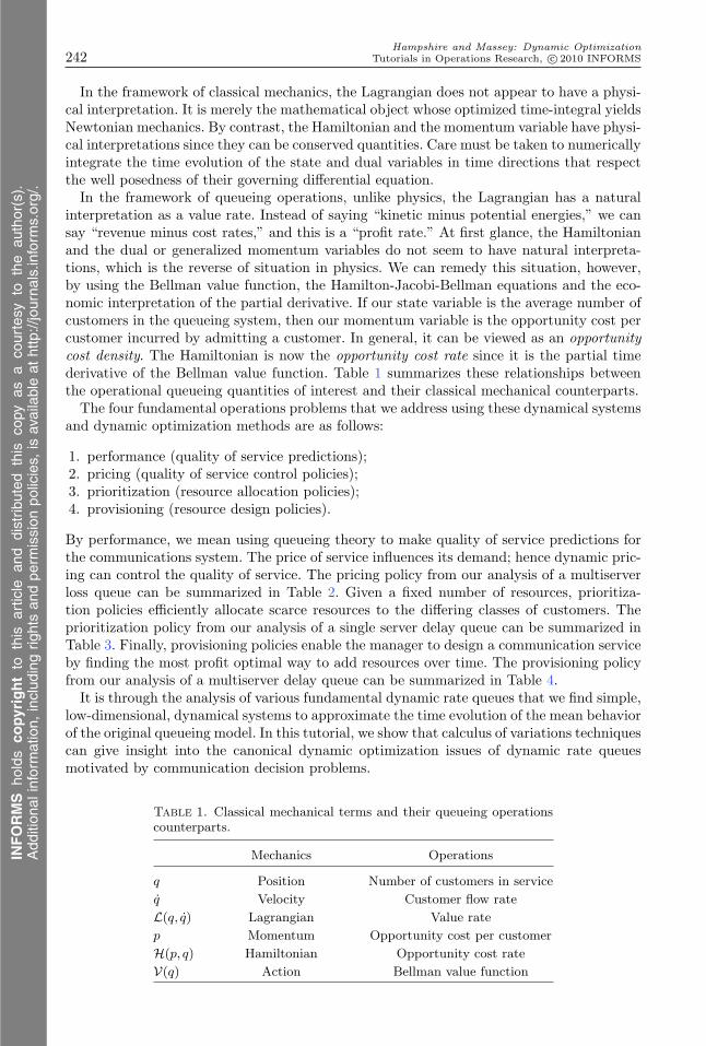
Hampshire and Massey: Dynamic Optimization242 Tutorials in Operations Research, c© 2010 INFORMS
In the framework of classical mechanics, the Lagrangian does not appear to have a physi-cal interpretation. It is merely the mathematical object whose optimized time-integral yieldsNewtonian mechanics. By contrast, the Hamiltonian and the momentum variable have physi-cal interpretations since they can be conserved quantities. Care must be taken to numericallyintegrate the time evolution of the state and dual variables in time directions that respectthe well posedness of their governing differential equation.In the framework of queueing operations, unlike physics, the Lagrangian has a natural
interpretation as a value rate. Instead of saying “kinetic minus potential energies,” we cansay “revenue minus cost rates,” and this is a “profit rate.” At first glance, the Hamiltonianand the dual or generalized momentum variables do not seem to have natural interpreta-tions, which is the reverse of situation in physics. We can remedy this situation, however,by using the Bellman value function, the Hamilton-Jacobi-Bellman equations and the eco-nomic interpretation of the partial derivative. If our state variable is the average number ofcustomers in the queueing system, then our momentum variable is the opportunity cost percustomer incurred by admitting a customer. In general, it can be viewed as an opportunitycost density. The Hamiltonian is now the opportunity cost rate since it is the partial timederivative of the Bellman value function. Table 1 summarizes these relationships betweenthe operational queueing quantities of interest and their classical mechanical counterparts.The four fundamental operations problems that we address using these dynamical systems
and dynamic optimization methods are as follows:
1. performance (quality of service predictions);2. pricing (quality of service control policies);3. prioritization (resource allocation policies);4. provisioning (resource design policies).
By performance, we mean using queueing theory to make quality of service predictions forthe communications system. The price of service influences its demand; hence dynamic pric-ing can control the quality of service. The pricing policy from our analysis of a multiserverloss queue can be summarized in Table 2. Given a fixed number of resources, prioritiza-tion policies efficiently allocate scarce resources to the differing classes of customers. Theprioritization policy from our analysis of a single server delay queue can be summarized inTable 3. Finally, provisioning policies enable the manager to design a communication serviceby finding the most profit optimal way to add resources over time. The provisioning policyfrom our analysis of a multiserver delay queue can be summarized in Table 4.It is through the analysis of various fundamental dynamic rate queues that we find simple,
low-dimensional, dynamical systems to approximate the time evolution of the mean behaviorof the original queueing model. In this tutorial, we show that calculus of variations techniquescan give insight into the canonical dynamic optimization issues of dynamic rate queuesmotivated by communication decision problems.
Table 1. Classical mechanical terms and their queueing operationscounterparts.
Mechanics Operations
q Position Number of customers in serviceq Velocity Customer flow rateL(q, q) Lagrangian Value ratep Momentum Opportunity cost per customerH(p, q) Hamiltonian Opportunity cost rateV(q) Action Bellman value function
INFORMS
holds
copyrightto
this
article
and
distrib
uted
this
copy
asa
courtesy
tothe
author(s).
Add
ition
alinform
ation,
includ
ingrig
htsan
dpe
rmission
policies,
isav
ailableat
http://journa
ls.in
form
s.org/.

Hampshire and Massey: Dynamic OptimizationTutorials in Operations Research, c© 2010 INFORMS 243
Table 2. Pricing policy for a multiserver loss queue.
Time Dual State Control Multiplier Slackregion variable variable variable variable variable
q∗ < θ p∗ = µ · p∗ q∗ = λ(π∗)− µ · q∗ λ(π∗) = (p∗ − π∗) x∗ = 0 y2∗ = θ − q∗
· λ′(π∗)q∗ = θ p∗ = µ · p∗ − x∗ q∗ =−(µ · q∗ − λ(π∗))+ π∗ = λ−1(µ · θ) x∗ = µ y∗ = 0
· (π∗ +1/λ′(π∗))
Table 3. Prioritization policy for a single server delay queue.
Opportunity cost Dual State Controlrate minimum variable variable variable
H1(p∗,q∗,w∗) p(1)∗ = (p(1)
∗ + r1) · θ(1)∗ (t) q
(1)∗ = λ1 − µ1 · q(1)
∗ w(1)∗ = 1− w0
· (1− θ(1)∗ (t)/µ1) q
(2)∗ = λ2 w
(2)∗ = 0
p(2)∗ = 0
p(1)∗ = 0 q
(1)∗ = λ1 w
(1)∗ = 0
H2(p∗,q∗,w∗) p(2)∗ = (p(2)
∗ + r2) · θ(2)∗ (t) q
(2)∗ = λ2 − µ2 · q(2)
∗ w(2)∗ = 1− w0
· (1− θ(2)∗ (t)/µ2)
Table 4. Provisioning policy for a multiserver delay queue.
Opportunity cost Dual State Controlrate minimum variable variable variable
H1(p∗, q∗) p∗ = 0 q∗ = λ C∗ = 0H2(p∗, q∗) p∗ = µ · (p∗ + r)− w′(q∗) q∗ = λ − µ · q∗ C∗ = q∗
Appendix. Linear Dynamical Systems and Markov Processes
Matrix ExponentialsOrdinary differential equations that only involve first derivatives are not as limiting as mightfirst appear. Consider the following example.
Problem 7 (Linear Ordinary Differential Equations). Consider the differentiablefunction x: [0, T ]→ R that solves the nth order ordinary differential equation
a0 ·x(t)+ a1 · dxdt
(t)+ · · ·+ an · dnx
dtn(t) = 0. (30)
Rewrite this equation as a linear function of q and ddtq.
Solution. If we define q(t), where
q(t) =[x(t),
dx
dt(t), . . . ,
dn−1x
dtn−1 (t)],
then we can rewrite (30) as
d
dtq(t) = q(t) ·A, (31)
INFORMS
holds
copyrightto
this
article
and
distrib
uted
this
copy
asa
courtesy
tothe
author(s).
Add
ition
alinform
ation,
includ
ingrig
htsan
dpe
rmission
policies,
isav
ailableat
http://journa
ls.in
form
s.org/.

Hampshire and Massey: Dynamic Optimization244 Tutorials in Operations Research, c© 2010 INFORMS
where
A=
0 0 0 · · · 0 −a0/an1 0 0 · · · 0 −a1/an0 1 0 · · · 0 −a2/an...
. . . . . . . . ....
...
0 0 0. . . 0 −an−2/an
0 0 0 · · · 1 −an−1/an
.
The deterministic process q(t) | t≥ 0 is referred to as a linear dynamical system. Moreover,it has the explicit solution of
q(t) = q(0) · exp(tA),
where the square matrix factor is called the matrix exponential or
exp(tA) =∞∑n=0
tn
n!An.
It is important to note that if the coefficients of the ordinary differential equation (or thematrix A) are time dependent, then the solution to q(t) is not the matrix exponential ofthe integral of the family of matrices A(s) |0 ≤ s ≤ t. This means that, in general, thesolution to
d
dtq(t) = q(t) ·A(t) (32)
is not the matrix exponential of the integral of this family of matrices or
q(t) = q(0) · exp(∫ t
0A(s)ds
).
We can make this concept work, however, by using the convention of time-ordered opera-tors due to Feynman [10]. First, define A(s) |0≤ s≤ t to be a family of formal matriceswith the property that for all pairs of times r < s, we have
A(r) · A(s) = A(s) · A(r)≡ A(r) ·A(s).
Now we can write our solution to (32), as the formal expression
q(t) = q(0) · exp(∫ t
0A(s)ds
).
Uniformization and Uniform AccelerationFor the case of a Markov process, the time evolution of the probability of being in a specificstate is a dynamical system. These are also called the Kolmogorov forward equations. Thegoverning matrix A is referred to as a Markov generator. Such generators have positiveoff-diagonal entries and row sums equal to zero. Assuming that all the diagonal terms overthe interval (0, t] are bounded by a constant α, then we define the matrix Pα(s) to be
Pα(s)≡ I+1αA(s)
INFORMS
holds
copyrightto
this
article
and
distrib
uted
this
copy
asa
courtesy
tothe
author(s).
Add
ition
alinform
ation,
includ
ingrig
htsan
dpe
rmission
policies,
isav
ailableat
http://journa
ls.in
form
s.org/.

Hampshire and Massey: Dynamic OptimizationTutorials in Operations Research, c© 2010 INFORMS 245
for all 0 ≤ s≤ t, where I is the identity matrix. These are called stochastic matrices wheretheir entries are positive and row sums equal one. Using our operator convention and lettingPα(t) be the time-ordered analogue to the stochastic matrix Pα(t) at time t, we have
exp(∫ t
0A(s)ds
)= exp
(−αt I+
∫ t
0αI+ A(s)ds
)= e−αt · exp
(αt · 1
t
∫ t
0Pα(s)ds
)=
∞∑n=0
e−αt · (αt)nn!
(1t
∫ t
0Pα(s)ds
)n=
∞∑n=0
e−αt · (αt)nn!
· n!tn
·∫
· · ·∫
0<s1<···<sn<t
Pα(s1) · · · Pα(sn)ds1 · · ·dsn
=∞∑n=0
e−αt · (αt)nn!
·∫
· · ·∫
0<s1<···<sn<t
Pα(s1) · · ·Pα(sn) · n!tnds1 · · ·dsn.
We now show that deeper results for Poisson processes give this sum a probabilistic inter-pretation.The lead scalar factor for each summand is the probability of a Poisson process making
n jumps during the interval (0, t]. A homogeneous Poisson process has the property thatconditioned on this event, the joint distribution of the n jump times equals the same forthe order statistics of n i.i.d. random variables that are uniformly distributed on (0, t]. Thismeans that the sample paths of this time-inhomogeneous Markov process are driven by thejumps of a Poisson process with rate α. At precisely these jump times, the process makes aninstantaneous transition according to a time-inhomogeneous Markov chains whose stochasticmatrices are specified by the time of the Poisson jump.In turn, this sample path decomposition, called uniformization, yields a sample path
interpretation of uniform acceleration. For a given scale parameter η > 0, we have
exp(∫ t
0η · A(s)ds
)=
∞∑n=0
e−ηαt · (ηαt)nn!
∫· · ·∫
0<s1<···<sn<t
Pα(s1) · · ·Pα(sn) · n!tnds1 · · ·dsn.
From this representation, we see that uniform acceleration speeds up the jump rate of theunderlying Poisson process but does not change the stochastic matrices sampled at any ofthe jump times.
References[1] C. E. Agnew. Dynamic modeling and control of congestion-prone systems. Operations Research
24 400–419, 1976.[2] J. M. Alden and R. L. Smith. Rolling horizon procedures in nonhomogeneous Markov decision
processes. Operations Research 40:183–194, 1992.[3] J. C. Bean, W. J. Hopp, and I. Duenyas. A stopping rule for forecast horizons in nonhomoge-
neous Markov decision processes. Operations Research 40:1188–1199, 1992.[4] R. Bellman. Dynamic Programming. Princeton University Press, Princeton, NJ, 1957.[5] D. P. Bertsekas. Dynamic programming and optimal control. Athena Scientific. Belmont, MA,
2001.[6] S. Eick, W. A. Massey, and W. Whitt. The physics of the M(t)/G/∞ queue. Operations
Research 41:400–408, 1993.[7] A. K. Erlang. Solutions of some problems in the theory of probabilities of significance in auto-
matic telephone exchanges. The Post Office Electrical Engineers’ Journal 10:189–197, 1918.[Originally published in Danish. +Elektroteknikeren 13, 1917].
INFORMS
holds
copyrightto
this
article
and
distrib
uted
this
copy
asa
courtesy
tothe
author(s).
Add
ition
alinform
ation,
includ
ingrig
htsan
dpe
rmission
policies,
isav
ailableat
http://journa
ls.in
form
s.org/.

Hampshire and Massey: Dynamic Optimization246 Tutorials in Operations Research, c© 2010 INFORMS
[8] S. N. Ethier and T. G. Kurtz. Markov Process: Characterization and Convergence. John Wiley& Sons, New York, 1986.
[9] G. M. Ewing. Calculus of Variations with Applications. Dover Publications, New York, 1985.[10] R. P. Feynman. The principle of least action in quantum mechanics. Unpublished doctoral
dissertation, Princeton University, Princeton, NJ, 1942.[11] M. C. Fu, T. G. Marcus, and I. Wang. Monotone optimal policies for a transient queueing
staffing problem. Operations Research 48:327–331, 2000.[12] L. Green and P. Kolesar. The pointwise stationary approximation for queues with nonstation-
ary arrivals. Management Science 37:84–97, 1991.[13] S. Halfin and W. Whitt. Heavy-traffic limits theorem for queues with many exponential servers.
Operations Research 29:567–588, 1981.[14] R. C. Hampshire. Dynamic queueing models for the operations management of communication
services. Unpublished doctoral dissertation, Princeton University, Princeton, NJ, 2007.[15] R. C. Hampshire and W. A. Massey. Variational optimization for call center staffing. Richard
Tapia Celebration of Diversity in Computing, Proceedings of the 2005 Conference on Diversityin Computing, Albuquerque, NM, 2005.
[16] R. C. Hampshire and W. A. Massey. Priority scheduling for a weighted processor sharing queuewith time varying rates. Working paper, Carnegie Mellon University, Pittsburgh, 2010.
[17] R. C. Hampshire, M. Harchol-Balter, and W. A. Massey. Fluid and diffusion limits for transientsojourn times of processor sharing queues with time varying rates. Queueing Systems 53:19–30,2006.
[18] R. C. Hampshire, O. B. Jennings, and W. A. Massey. A time varying call center design withLagrangian mechanics. Probability in the Engineering and Informational Sciences 23:231–259,2009.
[19] R. C. Hampshire, W. A. Massey, and Q. Wang. Dynamic pricing to control loss systemswith quality of service targets. Probability in the Engineering and Informational Sciences23:357–383, 2009.
[20] R. C. Hampshire, W. A. Massey, D. Mitra, and Q. Wang. Provisioning of bandwidth sharingand exchange. Telecommunications Network Design and Economics and Management: SelectedProceedings of the 6th INFORMS Telecommunications Conferences, Kluwer Academic Pub-lishers, Boston/Dordrecht/London, 207–226, 2002.
[21] W. J. Hopp. Technical note—Identifying forecast horizons for non-homogenous Markov deci-sion processes. Operations Research 37:339–343, 1989.
[22] W. J. Hopp, J. C. Bean, and R. L. Smith. A new optimality criterion for nonhomogeneousMarkov decision processes. Operations Research 35:875–883, 1987.
[23] R. L. Horne, A. Mandelbaum, and W. A. Massey. Large scale dynamics for multi-server queues.Working paper, Prenceton University, Princeton, NJ, 2010.
[24] D. L. Jagerman. Some properties of the Erlang loss function. Bell System Technical Journal53:525–551, 1974.
[25] D. L. Jagerman. Nonstationary blocking in telephone traffic. Bell System Technical Journal625–661, 1975.
[26] M. I. Kamien and N. L. Schwartz. Dynamic Optimization: The Calculus of Variations andOptimal Control in Economics and Management. Elsevier, Amsterdam, 1991.
[27] F. P. Kelly. Reversibility and Stochastic Networks. John Wiley & Sons, Chichester, UK, 1979.[28] L. Kleinrock. Queueing systems. Volume I: Queueing Systems. John Wiley & Sons, 1976.[29] J. Kolmos, P. Major, and G. Tusnady. An approximation of partial sums of independent RV’-s,
and the sample DF. II. Z.Wahrscheinlichkeitstheorie verw. Gebiete 32:111–131, 1975.[30] C. Lanczos. The Variational Principles of Mechanics, 4th ed. Dover Publications, New York,
1970.[31] M. Lewis and S. Yoon. Optimal pricing and admission control in a queueing system with
periodically varying parameters. Queueing Systems: Theory and Applications 47:177–199, 2004.[32] A. Mandelbaum and W. A. Massey. Strong approximations for time-dependent queues. Math-
ematics of Operations Research 20:33–64, 1995.[33] A. Mandelbaum, W. A. Massey, and M. Reiman. Strong approximations for Markovian service
networks. Queueing Systems 30:149–201, 1998.[34] J. Marsden and T. Ratiu. Introduction to Mechanics and Symmetry. Springer, New York, 1994.
INFORMS
holds
copyrightto
this
article
and
distrib
uted
this
copy
asa
courtesy
tothe
author(s).
Add
ition
alinform
ation,
includ
ingrig
htsan
dpe
rmission
policies,
isav
ailableat
http://journa
ls.in
form
s.org/.
Hampshire and Massey: Dynamic OptimizationTutorials in Operations Research, c© 2010 INFORMS 247
[35] W. A. Massey. Nonstationary queues. Unpublished doctoral dissertation, Stanford University,Stanford, CA, 1981.
[36] W. A. Massey. Asymptotic analysis of the time dependent M/M/1 queue. Mathematics ofOperations Research 10:305–327, 1985.
[37] W. A. Massey and W. Whitt. An analysis of the modified offered load approximation for thenonstationary Erlang loss model. Annals of Applied Probability 4:1145–1160, 1994.
[38] W. A. Massey and W. Whitt. Uniform acceleration expansions for Markov chains with time-varying rates. Annals of Applied Probability 8:1130–1155, 1998.
[39] B. L. Miller. Finite state continuous time Markov decision processes with finite planning hori-zon. SIAM J. Control 6:266–280, 1968.
[40] P. Pedregal. Introduction to Optimization (Texts in Applied Mathematics). Springer Science +Business Media, New York, 2004.
[41] L. S. Pontryagin, V. G. Boltyanshii, R. V. Gamkredlidze, and E. F. Mishchenko. The Mathe-matical Theory of Optimal Processes. John Wiley & Sons, New York, 1962.
[42] A. Prekopa. On Poisson and composed Poisson stochastic set functions. Studia Mathematica16:142–155, 1957.
[43] M. L. Puterman. Markov Decision Processes: Discrete Stochastic Dynamic Programming. JohnWiley & Sons, Chichester, UK, 1994.
[44] R. Sato and R. V. Ramachandran. Symmetry and Economic Invariance: An Introduction(Research Monographs in Japan-U.S. Business and Economics). Kluwer Academic Publishers,Norwell, MA, 1998.
[45] L. I. Sennott. Stochastic Dynamic Programming and the Control of Queueing Systems. Wiley-Interscience, New York, 1999.
[46] S. P. Sethi and G. Thompson. Optimal Control Theory: Applications to Management Scienceand Economics. Springer-Verlag, New York, 2000.
[47] S. Zeltyn and A. Mandelbaum. Call centers with impatient customers: Many-server asymptoticsof the M/M/n+G queue. Queueing Systems, Vol. 51. Springer, New York, 2005.
INFORMS
holds
copyrightto
this
article
and
distrib
uted
this
copy
asa
courtesy
tothe
author(s).
Add
ition
alinform
ation,
includ
ingrig
htsan
dpe
rmission
policies,
isav
ailableat
http://journa
ls.in
form
s.org/.


