Dynamic Optical Resource Allocation in Transport Networks ...kth.diva-portal.org/smash/get/diva2:1096090/FULLTEXT01.pdf · i Abstract Mobile traffic increases rapidly. Based on Ericsson’s

IN DEGREE PROJECT INFORMATION AND COMMUNICATION TECHNOLOGY,SECOND CYCLE, 30 CREDITS

, STOCKHOLM SWEDEN 2017

Dynamic Optical ResourceAllocation in Transport Networks Based on Mobile Traffic Patterns

EPAMEINONDAS KONTOTHANASIS

KTH ROYAL INSTITUTE OF TECHNOLOGYSCHOOL OF INFORMATION AND COMMUNICATION TECHNOLOGY

DEGREE PROJECT, IN COMMUNICATION SYSTEMS

PROGRAMME, SECOND LEVEL

STOCKHOLM, SWEDEN 2017

Dynamic Optical Resource

Allocation in Transport Networks

Based on Mobile Traffic Patterns

Author: Epameinondas Kontothanasis

School of Information and Communication Technology (ICT) KTH Royal Institute of

Technology Stockholm, Sweden

Dynamic Optical Resource

Allocation in Transport Networks

Based on Mobile Traffic Patterns

Epameinondas Kontothanasis, [email protected]

Master’s Thesis

Examiner Supervisor

Paolo Monti, PhD Matteo Fiorani, PhD

mailto:[email protected]

i

Abstract

Mobile traffic increases rapidly. Based on Ericsson’s forecast [1], mobile traffic is expected

to grow at a compound annual growth rate on percentage of 45% as the number of

smartphone subscriptions and the consumption per subscriber increase. The monthly data

traffic volume is expected to grow 6 times between 2015 and 2021. As demand increases,

new technologies are investigated and deployed to cover the user requirements. Intense

effort is given by researchers for the arrival of fifth generation (5G) network. High

performance and increased capacity requirements drive research to heterogeneous

networks. With the term “heterogeneous network”, a network that consists of different

technologies and architectures is described. A heterogeneous wireless network involves the

combination of macro and micro cells to improve coverage and capacity. All the traffic

generated from the mobile network should be transferred from the antenna, through an

access network, to the main office and from there to the backbone network. Optical

networks are considered as the ideal solution for this purpose and research drives

technology towards the usage of optical networks in the Fixed Mobile Convergence (FMC)

architectures. The FMC architectures are proposed architectures [2] that focus to converge

the fixed, mobile access and aggregation networks into a single transport network.

In this study, we analyze the FMC architecture. We particularly analyze the Fronthaul

architecture in combination with transport technologies such as Next Generation – Passive

Optical Network 2 (NG-PON2) and Wavelength Routed Wavelength Division Multiplexing

PON (WR-WDM-PON). We also take under consideration traffic patterns of mobile networks

generated in various urban areas in the city of Stockholm, based in different use of land.

Based on the traffic pattern, the number of small cells needed per area is calculated.

In this thesis project, the traffic patterns from the mobile network and the transport

network architectures are studied. The purpose of this thesis is to create an algorithm and

study different sharing scenarios of the underlying transport infrastructure. The results of

this algorithm will reveal if sharing and reusing resources in the transport infrastructure is

beneficial in terms of saving resources.

ii

Sammanfattning

Mobiltrafik ökar snabbt. Baserat på Ericssons prognos [1], väntas mobiltrafiken få en årlig tillväxttakt på 45% i samband med att antalet smartphone-abonnemang och förbrukning per abonnent ökar. Den månatliga volymen av datatrafik väntas att öka sexfaldigt mellan 2015 och 2021. Allteftersom efterfrågan ökar, undersöks och distribueras ny teknik för att möta användarnas krav. Intensivt forskningsarbetearbete bedrivs inför av femte generationens (5G) nätverk. Högt ställda krav på prestanda och kapacitet är de drivande faktorerna i forskningen av heterogena nätverk. Med heterogena nätverk menas nätverk som består av olika teknologier och arkitekturer. Ett heterogent trådlöst nätverk involverar kombinationen av makro- och mimkroceller för att förbättra täckning och kapacitet. All trafik som genereras i mobila nätverk ska överföras från antennen, genom ett accessnät, till huvudkontoret, och därifrån till backbone-nätverket. Optiska nätverk betraktas som den idealiska lösningen för detta ändamål, och forskare driver teknologin mot användning av optiska nätverk i Fixed Mobile Convergence- (FMC) arkitekturer. FMC arktekturer är föreslagna arkitekturerna som fokuserar på att konvergera fasta, mobila och aggregerings-nätverk till ett enda transportnät. I denna studie, analyserar vi FMC-arkitekturen. Vi analyserar särskilt Fronthaul-arkitekturen i kombination med transportteknologier, så som Next Generation - Passive Optical Network 2 (NG-PON2) och Wavelength Routed Wavelength Division Multiplexing PON (WR-WDM-PON). Vi tar också hänsyn till trafikmönster i mobila nätverk i olika sorters urbana områden i Stockholm. Baserat på trafikmönstret räknas antalet små celler som behövs per område ut. I detta examensarbete är det trafikmönster från mobila nätverk och transportnätverksarkitekturer som studeras. Syftet med denna avhandling är att skapa en algoritm, och studera olika olika scenarion där den underliggande transportinfrastrukturens resurser delas. Resultatet av denna algoritm avslöjar om delning och återanvändning av resurser i transportnätverket är fördelaktigt när det gäller att spara resurser.

iii

Acknowledgements

At this point I would like to thank the people who helped me, in different ways during this master

thesis.

Paolo Monti, who is my examiner, for accepting working with me during the master thesis

and guided me through the thesis. Also, his help in administrative issues helped me to

complete this project.

Matteo Fiorani, my supervisor. Matteo guided me through the project step by step and help

me understand all the different concepts of the project.

Family, especially my sister, and friends, especial Sundus and Theodor, who supported me

and stood by me during the project

Sincerely,

Epameinondas Kontothanasis

September 2017

iv

List of Figures Figure 1: Backhaul transport network [2] ............................................................................................................... 8

Figure 2: NG-PON2 with PtP WDM overlay [38] ................................................................................................... 10

Figure 3: Logical architecture of a generic PtP WDM PON [7] .............................................................................. 11

Figure 4: System diagram of the filtered WDM-PON solution using a cyclic AWG at the remote node [1] ......... 12

Figure 5: System setup – component level view [1] ............................................................................................. 13

Figure 6: NG-PON2 Shared spectrum with flexible WDM-PtP wavelength allocation [2] .................................... 15

Figure 7: Flexible DWDM-centric access network based on WSSs [2] .................................................................. 16

Figure 8: Capacity contribution of small cells and Wi-Fi as the density of small cells increases [31] ................... 19

Figure 9: Base Stations in Stockholm City Center [30] .......................................................................................... 20

Figure 10: Base Stations in Area of Kista, Stockholm [30] .................................................................................... 20

Figure 11: Traffic pattern in Office area [34] ........................................................................................................ 21

Figure 12: Traffic pattern in Resident area [34].................................................................................................... 21

Figure 13: Traffic pattern in Transport area [34] .................................................................................................. 21

Figure 14: Combination of normalized traffic on weekdays for Office/Transport areas [34] .............................. 22

Figure 15: Combination of normalized traffic on weekends for Office/Transport areas [34] .............................. 22

Figure 16: Combination of normalized traffic on weekdays for Resident/Transport areas [34] .......................... 22

Figure 17: Combination of normalized traffic on weekends for Resident/Transport areas [34] ......................... 22

Figure 18: Summarization of traffic pattern – weekday ....................................................................................... 24

Figure 19: Summarization of traffic pattern – weekend ...................................................................................... 24

Figure 20: Shared infrastructure between all three areas – NG-PON2 large network ......................................... 36

Figure 21: Shared infrastructure between all three areas – WR-WDM-PON large network ................................ 37

Figure 22: Shared infrastructure between all three areas – NG-PON2 small network......................................... 38

Figure 23: Shared infrastructure between all three areas – WR-WDM-PON small network ............................... 38

Figure 24: Shared infrastructure between transport and resident areas – NG-PON2 large network .................. 40

Figure 25: Shared infrastructure between transport and resident areas – WR-WDM-PON large network ......... 41

Figure 26: Shared infrastructure between transport and resident areas – NG-PON2 small network .................. 42

Figure 27: Shared infrastructure between transport and resident areas – WR-WDM-PON small network ........ 43

Figure 28: Shared infrastructure between transport and office areas – NG-PON2 large network ...................... 44

Figure 29: Shared infrastructure between transport and office areas – WR-WDM-PON large network ............. 45

Figure 30: Shared infrastructure between transport and office areas – NG-PON2 small network ...................... 46

Figure 31: Shared infrastructure between transport and office areas – WR-WDM-PON small network ............. 46

Figure 32: Shared infrastructure between office and resident areas – NG-PON2 large network ........................ 48

Figure 33: Shared infrastructure between office and resident areas – WR-WDM-PON large network ............... 49

Figure 34: Shared infrastructure between office and resident areas – NG-PON2 small network ........................ 50

Figure 35: Shared infrastructure between office and resident areas – WR-WDM-PON small network .............. 50

v

List of Tables Table 1: Comparison for fronthaul [2] .................................................................................................................. 14

Table 2: Examples of base station densities (Urban areas in Sweden) [13] ......................................................... 18

Table 3: Summary of savings for non-sharing infrastructure during weekdays ................................................... 28

Table 4: Summary of savings for sharing infrastructure during weekdays ........................................................... 29

Table 5: Summary of savings for non-sharing infrastructure during weekends ................................................... 29

Table 6: Summary of savings for sharing infrastructure during weekends .......................................................... 29

List of Diagrams Diagram 1: Chart flow of algorithm ...................................................................................................................... 31

Diagram 2: Algorithm's chart flow for Case Study ................................................................................................ 33

vi

Contents Abstract ....................................................................................................................................... i

Sammanfattning......................................................................................................................... ii

Acknowledgements ................................................................................................................... iii

List of Figures ............................................................................................................................ iv

List of Tables .............................................................................................................................. v

List of Diagrams .......................................................................................................................... v

Contents .................................................................................................................................... vi

List of Acronyms ...................................................................................................................... viii

1. Introduction ........................................................................................................................... 1

1.1 Thesis Outline ................................................................................................................... 2

1.2 Ethical, Social and Environmental impact of thesis ......................................................... 2

2. Background ............................................................................................................................ 4

3. Problem Statement ................................................................................................................ 5

4. Related Work and Existing Technologies ............................................................................... 6

4.1 Related Work .................................................................................................................... 6

4.2 Technologies ..................................................................................................................... 7

4.2.1 FMC Fixed Mobile Convergence ................................................................................ 7

4.2.2 RAN Architectures ..................................................................................................... 7

4.2.2.1 Backhaul .............................................................................................................. 8

4.2.2.2 Fronthaul ............................................................................................................. 8

4.4 Optical Transport Networks ............................................................................................. 9

4.4.1 NG-PON2.................................................................................................................... 9

4.4.2. PtP WDM-PON ........................................................................................................ 11

4.4.2.1. WR-WDM-PON ................................................................................................. 11

4.4.2.2. WS-WDM-PON ................................................................................................. 13

4.5. Comparison between transport technologies for Fronthaul architecture ................... 13

4.5.1 Difference between NG-PON2 and WR-WDM-PON................................................ 13

4.5.2 Difference between WS-WDM-PON and WR-WDM-PON ....................................... 14

4.6. Transport Network Topologies ..................................................................................... 14

4.6.1 NG-PON2 with PtP-WDM shared spectrum ............................................................ 15

4.6.2 Flexible DWDM-PON ............................................................................................... 16

vii

5. Methodology ........................................................................................................................ 17

6. Implementation ................................................................................................................... 18

6.1 Mobile network design .................................................................................................. 18

6.2 Transport Network ......................................................................................................... 23

6.3 Data Collection ............................................................................................................... 24

6.3 Model – Algorithm ......................................................................................................... 29

6.3.1 Case Study implementation .................................................................................... 32

7. Results and Analysis ............................................................................................................. 35

7.1 Results ............................................................................................................................ 35

7.2 Summary of results ........................................................................................................ 52

8. Conclusions and Future Work .............................................................................................. 53

8.1 Conclusions ..................................................................................................................... 53

8.2 Future Work ................................................................................................................... 53

References ............................................................................................................................... 55

Appendix .................................................................................................................................. 58

viii

List of Acronyms 5G Fifth Generation

AON Active Optical Network

AWG Arrayed Waveguide Grating

BBU Base Band Unit

CO Central Office

CPRI Common Public Radio Interface

C-RAN Centralized Radio Access Network

DWDM Dense Wavelength Division Multiplexing

FMC Fixed Mobile Convergence

FTTC Fiber to the Cabinet

FTTH Fiber to the Home

LTE Long Term Evolution

LTE-A Long Term Evolution Advanced

MBS Mobile Base Station

NG-PON2 Next Generation Passive Optical Network 2

OADM Optical Add/Drop Multiplexers

OBSAI Open Base Station Architecture Initiative

ODN Optical Distribution Network

OLT Optical Line Termination

ONU Optical Network Unit

PON Passive Optical Network

PtP WDM Point-to-point Wavelength Division Multiplexing

RAN Radio Access Network

ROADM Reconfigurable Optical Add-Drop Multiplexer

RRU Remote Radio Unit

ix

RTT Roundtrip

RU Radio Unit

TWDM PON Time and Wavelength Division Multiplexing Passive Optical Network

WDM Wavelength Division Multiplexing

WDM-PON wave division multiplexing passive optical network

WR-WDM-PON Wavelength Routed Wavelength Division Multiplexing Passive Optical

Network

WS-WDM-PON Wavelength Selective Wavelength Division Multiplexing Passive Optical

Network

WSS Wavelength Selective Switch

1

1. Introduction

The Ericsson Mobility report states that “Every second, 20 new mobile broadband

subscriptions are activated” [1]. Mobile traffic increases every year. Based on the Ericsson’s

forecast [1], the mobile traffic is expected to grow at a compound annual growth rate on

percentage of 45%. This forecasted number derives from the expected increased number of

smartphone subscriptions and the increased data consumption per subscriber. The monthly

data traffic volume is expected to grow 6 times between 2015 and 2021. As the demand

increases, new technologies are investigated and deployed in order to cover the needs.

Intense effort is given by researchers for the arrival of fifth generation (5G) network. High

performance and increased capacity requirements drive research to heterogeneous

networks. With the term “heterogeneous network”, a network that consists of different

technologies and architectures is described. A heterogeneous network can involve the

combination of macro and micro cells in order to improve coverage and capacity. All traffic

generated from the mobile network should be transferred from the antenna, through an

access network, to the main office and from there to the backbone network. In addition,

research is in progress in order to converge mobile network and fixed network. In Combo

project deliverable 3.3 [2], a fixed mobile network convergence scenario is described. The

target is to combine those two networks under a common single infrastructure. Optical

networks are described as the ideal solution and research drives technology towards the

usage of optical networks in the Fixed Mobile Convergence (FMC) [2].

In this thesis we analyze the FMC architecture [2]. Especially we analyze the Fronthaul

architecture in combination with transport technologies such as Next Generation – Passive

Optical Network 2 (NG-PON2) and Wavelength Routed Wavelength Division Multiplexing

PON (WR-WDM-PON). The concept of the Fronthaul architecture is that the Base Band Unit

(BBU) and the Remote Radio Unit (RRU) are located in different locations. In this scenario,

when the BBU is moved from the Base station, the communication between the BBU and

the RRU is achieved using the Common Public Radio Interface (CPRI) protocol or other

protocols. Also, we take under consideration traffic patterns generated in different urban

areas in the city of Stockholm. From those traffic patterns, valuable data are extracted

about the usage of the transport network.

The thesis is based in the concept that we divide an urban area into different types such as

residential areas, where in majority consist of housing, office areas where is the business

district and transport areas where mainly means of transportation are present. For each

area, the traffic pattern of mobile usage is taken under consideration. Based on the traffic

pattern, the number of small cells that are needed per area is calculated. Having the total

number of small cells that are needed, the idea is to share the underlying transport

infrastructure in order to reuse the wavelengths and use the fewest small cells.

2

This thesis project focuses on examining if sharing resources and reusing resources is

beneficial in terms of cost. The research involves studying different optical network

architectures and transport/access topologies and analyzing traffic patterns generated by

the mobile network.

The goal of this thesis is to create an algorithm and study different sharing scenarios of the

underlying transport infrastructure. By sharing the transport network between different

types of areas we expect to save more resources, meaning that less small cells can be used

for serving the demanded traffic. To find the best combination of shared infrastructure for

using fewer devices, different sharing scenarios are taken under consideration. The

algorithm takes as input the traffic percentage in the base station and the number of small

cells in each area and the type of transport infrastructure and return as result the number of

small cells used in given time.

The results of this algorithm will reveal if sharing and reusing resources in the transport

infrastructure is beneficial in terms of saving resources.

1.1 Thesis Outline

The rest of this work is organized in 7 chapters. In chapter 2, an overview of the background

is provided. An overview of the optical networks in conjunction with the upcoming fifth

generation (5G) technology is also provided. In chapter 3 the initial problem statement is

described. Chapter 4 presents the related work in the field and an overview of related

existing technologies is presented. It continues by explaining already existing optical

transport technologies that will be taken under consideration in later stages. Chapter 5

explains the research methodology that has been followed in order to guide us in a concrete

conclusion. In chapter 6, we analyze how the data are collected, what technologies are

taken under consideration to build the algorithm and explain how the developed algorithm

works. In chapter 7, the experimental results about the usage of small cells are presented

and in chapter 8 the conclusions are given with the future work in order to continue this

study.

1.2 Ethical, Social and Environmental impact of thesis

The goal of this master thesis is to identify if dynamic allocation of optical resources in

transport networks is beneficial in terms of cost. The increasing number of devices, new

services and applications that require more bandwidth and the increasing number of

subscribers lead to higher volumes of requested data through the mobile network. The

upcoming technology of 5G network and the unified transport network will be able to

handle the big volume of traffic. The results of this thesis help improving the underlying

3

transport network. Creating a most robust network, that addresses the high demand of

traffic and satisfy the users’ needs have a beneficial social effect.

Due to ethical reasons and university ethics, the results are disclosed and are presented

unbiased. Also, any published details presented in this work are fully acknowledged based

on standard reference practices. The results of the thesis, allocating resources dynamically

based on traffic patterns, results less resources are used. Less small cells are active or

needed. Moreover, less equipment is needed in order to serve the same demand. The

reduced number of needed equipment has a positive impact on environment. By the time

that fewer devices are needed, less power consumption is required making the overall

solution more environmental friendly.

4

2. Background

Optical networks are capable of transferring high demanding services in big distances. One

of the architectures to deploy optical fiber to the access network is to use a point-to-point

network. Lines from the main office will end up to the optical network unit (ONU) in the

destination. In addition, using passive optical networks (PON), where no power is required,

to split signal from one source to multiple destinations in combination with wave division

multiplexing WDM technology, multiple wavelengths are supported for downstream or

upstream signals.

Optical networks are one of the means of transportation that can support the upcoming 5G

technology. The architecture where the processor unit (baseband unit – BBU) is

geographically separated from the RRU and centralized in a main Central Office (CO), is

referred as centralized Radio Access Network (C-RAN). The C-RAN has the potential to bring

several advantages with respect to current radio access networks. Cost efficiency as less

BBUs are used is one of the benefits. Also, rollout difficulties in dense urban areas are

limited in this design [3]. Another driver for this is the limited space in urban places.

Removing equipment from the antennas and centralizing those saves space in new

installations. Furthermore, C-RAN architecture enables features of LTE for better

coordination between neighboring cells [3].

Another aspect that should be considered in the C-RAN architecture is the communication

between the RRU and the BBU. So far, those two elements where geographically close, in

the same base station site. The communication between those elements is achieved

through the Common Public Radio Interface (CPRI).

The above design where the BBU is centralized and the communication between BBU and

RRU is achieved with the CPRI is referred to as Fronthaul network.

CPRI protocol is quite demanding in terms of bandwidth and latency and Dense Wavelength

Division Multiplexing (DWDM) is the technology of choice for transporting CPRI signals, due

to its high bandwidth as well as stringent latency/jitter requirements [3].

Today, the major DWDM switching technology is deployed using reconfigurable optical

add/drop multiplexers (ROADMs). ROADMs are used to automate the rearrangement of

wavelengths on multichannel fibers that enter and exit the nodes [4]. A Multi-Wavelength

Selective Switch (WSS) is a ROADM that selectively rearrange the wavelengths towards

different directions [5].

However, not only ROADMs are used. OADMs with fixed routing matrix are also used. One

switch that is used as well is called Arrayed Waveguide Grating (AWG).

5

3. Problem Statement

At the moment, the bandwidth allocation between the Radio Unit and the Baseband Unit is

fixed and equal to the peak demand. If there is a need for higher capacity and demand, new

small cells need to be installed in order to serve the capacity. This increases the cost of the

overall installations. However, reusing and sharing resources can be beneficial in terms of

cost. Been able to switch on/off the small cells based on the demand can save resources.

This creates the need for the transport network to work in a dynamic way. The transport

network needs to have the ability to dynamically allocate optical resources only to the

currently active small cells.

More specifically, traffic from different areas varies based on the movement of users, the

traffic patterns and the demand. The traffic pattern from different RRUs will fluctuate based

on place and time. At the same moment, not all RRUs require to be active in order to serve

the demand. This drives a dynamic allocation of resources where it is needed.

This dynamicity can be beneficial by dynamically allocating resources of C-RAN or

dynamically allocating resources in the transport network only to areas and small cells

where the traffic is needed. In advance, more savings can be achieved energy wise in both

radio and transport networks by powering off cells or interfaces in the transport network

that are not needed [2].

The goal is to study the mobile network usage and based on those patterns to evaluate the

dynamic resource allocation following the assumption that the small cells are not always in

on state. The savings would be significant for large installations of small cells as only a

number of cells need to be active in the same time.

6

4. Related Work and Existing Technologies

4.1 Related Work

A lot of research has been done in energy saving in 5G network and FMC. Energy saving in

the New Generation Network is a key factor in order to be efficient. Some related work to

energy saving solutions is presented below.

As studied in [6], the minimum number of BBUs to be installed in a network is analyzed.

More specific, in a WDM-PON network, they propose the most suitable placement for the

BBUs. In [7], the placement of BBUs in order to achieve more cost-efficient network is

studied. The study proposes a solution that saves up to 65% in dense-urban/urban

locations; however, the number of wavelengths used in each link is preconfigured and fixed.

Also, based on [7] Fronthaul traffic is not tolerant in latency and jitter and single point-to-

point links should be used to satisfy this demand.

In [8] is showed that PON network are more power efficient than active optical networks

(AON) or PtP networks.

In [9], the authors propose a design using passive splitter in the remote node where the

ONUs will form a virtual topology sharing a wavelength where the demand is limited. A

mathematical algorithm is proposed for the trade-off between energy saving and

wavelength reconfiguration.

In [10] an algorithm to dynamically switch on/off small cells is presented. In this work, the

author presents an equation for small cell placement and uses different traffic patterns that

are going to be analyzed. The small cell density Ds in 1/km2 is represented as:

𝐷𝑠 ≥ (𝐺(𝑡)𝑚𝑎𝑥(1 − 𝑃𝑜𝑢𝑡) − 𝐶𝑚

𝐶𝑠)

where G(t)max is the maximum traffic volume among test cases, Pout is the expected outage

probability, which is assumed here to be 0.05.The capacity values Cm and Cs, corresponding

to the macro cell capacity and small cell capacity, are derived from the assumptions of a

2.315 bps/Hz spectral efficiency and a bandwidth of 1 GHz.

In another work, [2], the number of small cells is defined as 10 small cells per macro cell

station, for the needs of the project. In order to connect the small cells, different

architectures have been studied. Wavelength Division Multiplexing - Passive Optical

Networks (WDM-PON) [11], [12] looks to be a serious candidate for FMC infrastructures.

In [13], a cost and capacity analysis for macro cell and femtocell is presented. What is

interesting in this work is the assumption of the bandwidth demand for a specific area. Also

the density for an area of interest is presented.

7

In a report from Senza Fili consulting [14], the increases capacity from the ratio small cell to

macro cell is presented. In this report, it is mentioned the linear increase of the capacity of

macro cell towers as the number of small cells attached increases.

In [15], even if they work mainly with capacity of the mobile network, the related and

interesting part is the system model that they use in order to simulate the mobile network.

Assumptions of this system will be taken under consideration in this project as well. In this

paper, is also mentioned the importance of switching off base stations where there is no

traffic. In a large network with many small cells, small cells can be powered off as the

number of users is decreased.

4.2 Technologies

4.2.1 FMC Fixed Mobile Convergence

So far different network types such as wired or fixed, Wi-Fi and mobile networks have been

developed in an autonomous way and their infrastructure is separated. Nowadays there is

some convergence but is partial. For the fixed access network, this convergence includes

aggregation of access equipment in the Main CO, and the deployment of a passive fiber

network towards the residential customers in a Fiber to the Cabinet (FTTC) or Fiber to the

Home (FTTH) approach [2]. In the fully converged network infrastructure, the network will

be shared for fixed and mobile access towards the core network.

With the FMC infrastructure, different solutions can be supported. One of those solutions is

the so called BBU hotelling [16, 17], where the baseband units are separated from the

remote radio heads and are consolidated in common locations, the “hotels” [7].

A preliminary work has been carried out in [18], where a simple multi-stage WDM-PON is

considered as FMC network and the number of deployed hotels is minimized.

4.2.2 RAN Architectures

Before proceeding to the RAN architecture, is useful to describe the main components of

the architectures.

Base Station: A Base Station consists or two parts. The one is the baseband unit (BBU) in

order to perform the digital data processing and the radio unit (RU) that performs the

analog radio processing and generates the radio signal that is transmitted thought the

antennas. The BBU and the RU are connected via optical fiber.

Macro Cell: A macro cell unit, in general is used for coverage.

Small Cell: While macro cellules are used to provide coverage, their capability of offering big

capacity is limited. In order to provide higher capacity to the network, densification of the

8

network is required. However, adding more macro cell stations will increase the cost and

interference between the stations. Small cellular base stations operating in the same

spectrum as the macro cell base stations solve the problem of high demand in capacity [19].

Their main use is to increase capacity while macro cell base station provides coverage [15].

However, there are some considerations about the deployment of small cells. The macro

network minimizes the interference between the sites. In the case of small cells, the

interference should be taken under consideration. In order to overcome this problem, the

transmission power is limited. Also, optimal placement should be designed in order to place

the stations close to the end users [14].

4.2.2.1 Backhaul

One of the RAN architectures is the called “backhaul architecture”. In the backhaul

architecture the BBU and the RRU are located in the same location – site. Then the data are

backhauled in the access network. The data that are carried can be separated in two types:

1. Data from the X2 interface. This interface is used for communication between the

eNBs for e.g. radio coordination. The roundtrip (RTT) should be less than 1ms

2. Data from Long Term Evolution Advanced (LTE-A) S1. This type concerns the user

traffic data.

The backhaul link capacity is the max of the sum of X2 data plus S1 data [2].

Figure 1: Backhaul transport network [2]

4.2.2.2 Fronthaul

The main difference with the backhaul architecture is that the BBU and the RRU are located

in different locations. However, the distance between the RRU and the BBU is a constrain

and the correct placement of the BBU should be considered [20]. The Common Public Radio

Interface (CPRI) [21] transport protocol is used for the communication between the BBU and

the RRU [3].

9

At the moment, CPRI is the most adopted protocol for the fronthaul architecture. However,

because of proprietary technologies and interoperability between vendors, still is not

possible [3]. Also even if CPRI is the most adopted protocol, open base station architecture

initiative (OBSAI) standard can also be used [22].

A big advantage of this architecture compared to backhaul is the reduction of the cost as

less BBU are required. The BBU is centralized instead of distributed; so many RRU can

connect to the same BBU.

Nevertheless, for this architecture there are some drawbacks. One drawback is the low

latency required between the processor and the radio unit. Another drawback for this is the

transport capacity required for the CPRI traffic [23].

In the architecture where several BBUs are centralized in the Main CO, the BBUs are inter-

connected (BBU Hotel). This inter-connectivity is used for the X2 links. The S1 traffic is

forwarded to the EPC.

In order to build a fronthaul transport network, some requirements should be taken into

consideration, as it is mentioned in [2]:

1. Radio Site Configuration: Radio sites can be classified in macro cells and micro or

small cells.

2. Data-Rate: CPRI is a constant bit-rate interface, whose data rates go from 614.4

Mbit/s up to 10.137 Gbit/s for LTE radio configurations.

3. Data-Rate Performance: the fronthaul segment must not degrade the radio

performance

4. Latency and Other Timing Parameters

5. Synchronization and Jitter

6. Fronthaul Monitoring

7. Business and Local Requirements [3]

4.4 Optical Transport Networks

4.4.1 NG-PON2

The overview of a NG-PON2 optical line terminal consists of two services for backward

compatibility. It consists of TWDM PON and PtP WDM shared spectrum. Based on [24], a

time and wavelength division multiplexing passive optical network (TWDM PON) is a

multiple wavelength PON solution in which each wavelength is shared between multiple

optical network units (ONUs) by employing time division multiplexing and multiple access

mechanisms and Point-to-point wavelength division multiplexing (PtP WDM) is a multiple

10

wavelength PON solution that provides a dedicated wavelength per ONU in both

downstream and upstream directions. The defining characteristic of a PtP WDM is that each

ONU is served by one or more dedicated wavelengths.

NG-PON2 offers convergence for all fixed and mobile networks and also allows reusing the

existing network resources. Also, it can be operated as a PtP WDM overlay for shared

spectrum or dedicated PtP WDM for expanded spectrum [2]. Using point-to-point WDM

wavelengths, gives the possibility to use up to 16 bi-directional channels to transport the

CPRI to the BBUH from the RRU. This technology is based on tunable lasers [2]. As far as the

reach concerns, NG-PON2 should be able to cover distance of 40km without any extenders

or 60km using extenders.

Figure 2: NG-PON2 with PtP WDM overlay [25]

The ONU in the destination uses tunable laser, a prerequisite for per-channel capacity and

reach.

In the case of NG-PON2 overlay, 1:16 AWG are deployed as there is a restriction in the

number of wavelength shared in the fiber in contrast with WDM-PON where 1:80 AWG are

used. However, in NG-PON2 the fibers can be reused leading to reduced fiber cost.

Selective OLT port sleep for power saving during low traffic periods. During times of low

traffic load (e.g. overnight) all ONUs can retune to a common wavelength and allow OLT

ports to be powered down [26].

11

4.4.2. PtP WDM-PON

In the PtP WDM-PON solution, on the OLT side, wavelengths are multiplexed onto a bi-

directional fiber. This connects the wavelength multiplexer to a branching node [26].

Figure 3: Logical architecture of a generic PtP WDM PON [26]

Different combinations of wavelength filters such as AWGs or power splitters or

bandpass/bandstop filters can be included in the branching node. Between the colorless

ONU transceiver and the branching node, a wavelength selection function is required [26].

This wavelength selector can be placed within the optical network unit or at the branching

node. In the first case where the selector is placed in the ONU we have the wavelength

selected case (WS-WDM-PON) while in the second case we have the wavelength routed

(WR-WDM-PON) [26].

4.4.2.1. WR-WDM-PON

A directly-detected, wavelength-routed runs via filters like AWG instead of power splitters

and uses tunable lasers at the ONUs and multichannel transceiver arrays at the OLT. The C-

band tunable lasers, allows for longer reach and higher capacity in the WR. In contrast with

the NG-PON2 PtP WDM that supports 16 wavelengths, WR-WDM-PON can support 80 bi-

directional channels using for upstream the C-Band and for the downstream the L-Band

[27]. However, using cyclic AWGs or AWGs with flat-top transmission characteristics can

achieve the number of 320 clients [27]. Another way to increase the client-count is to re-

use the downstream wavelength. The ONU can re-use the downstream wavelength as the

upstream wavelength. In addition, adding a second AWG (2 x 80:1 AWGs) the number of

clients can increase to 160 [27]. However, this solution is not cost efficient. Instead, 48:1

AWG can be used offering in total the capability of 96 clients.

12

In the branching node is the λ selection function as well. The wavelength of the colorless

ONU is selected by the connectivity to the ODN. In addition, the wavelengths for upstream

and downstream traffic may differ [26].

Figure 4: System diagram of the filtered WDM-PON solution using a cyclic AWG at the remote node [28]

In order to route wavelengths to an ONU, a WDM multi/demultiplexer is used. A specific

wavelength is routed downstream to an ONU by an AWG and another upstream to the

central office. Wavelength routing is performed by static filters, e.g. Optical Add/Drop

Multiplexers (OADM) or Reconfigurable OADM (ROADM) [2]. This solution is suitable to

the requirements of a converged access/backhaul/fronthaul infrastructure for

bandwidth up to 10Gb/s per wavelength reaching in distance 50km due to the use of

filters [1]. In order to support up to 80 bi-directional (symmetrical) devices, a low cost

tunable laser is deployed in each ONU. The ONU in the destination uses tunable laser, a

prerequisite for per-channel capacity and reach. It uses the C-band for upstream and L-

band for downstream traffic and is a key component of the filtered WDM-PON [28].

In advance, one of the main requirements is to achieve auto-tuning of the ONU. To

achieve this goal, a centralized wavelength control is needed [28]

13

Figure 5: System setup – component level view [28]

In another work [2], in order to connect the Mobile Base-Station (MBS), a WR-WDM-PON

fronthaul is selected. The benefits comparing to the PtP WDM overlay is the number of

wavelengths that are available. In this case, an AWG is used at each MBS.

4.4.2.2. WS-WDM-PON

In the scenario of wavelength selected WDM PON, the wavelength selection is performed in

the ONU. The ONU and the OLT can communicate on part or the entire spectrum as they are

available in the ONU [26]. However, WS is more complex and costly than WR variant due to

tunable filter. It requires a power budget of 33-35 dB for splitting ratios of 1:32 and covering

distance 20km. Also, the interferometric crosstalk can limit the number of channels, which is

especially critical in the upstream link [28]. Also, the WS-ODN does not make use of WDM.

They inly separate upstream from downstream. WS-WDM-PON supports 64 bi-directional

channels (2*64 wavelengths in L-band and C-band) [2].

4.5. Comparison between transport technologies for Fronthaul architecture

In this section, the basic differences between the transport technologies are presented.

4.5.1 Difference between NG-PON2 and WR-WDM-PON

The main difference is that in NG-PON2, micro cells and residential Wi-Fi access is through

power splitters while in WR-WDM-PON are through filters.

14

4.5.2 Difference between WS-WDM-PON and WR-WDM-PON

Apart from the difference between filters and power splitters, another difference is the use

of and the number of amplifiers used in the WS.

Table 1: Comparison for fronthaul [2]

The table above presents a comparison between fronthaul solutions that discussed earlier.

The table compares elements and components needed as well as system latency and length

of fibers needed [2]. The number of amplifiers needed in NG-PON-2 solution is much higher

than the number of amplifiers needed in WR-WDM-PON solution (zero amplifiers are

needed). The amplifiers are needed to restore the signal strength. Optical components, e.g.

multiplexers, add loss and after a distance the signal becomes too weak. So, in order to

reach higher distances, NG-PON2 and WS-WDM-PON, most likely need the use of amplifiers.

Also, the number of the total passive optic elements is higher in NG-PON2 than the other

two solutions. However, the number of the fibers needed in the WR-WDM-PON is higher

that the NG-PON2 solution.

4.6. Transport Network Topologies

The described before, fronthaul service, can be provided either using NG-PON2 or WR-

WDM-PON. In the case of NG-PON2, the access OLT node, remain in the Main CO because of

the latency requirements to carry the CPRI traffic. Up to 16 bi-directional channels can be

served by an additional set of PtP WDM overlay on top of the TDM/TDMA set that is shared

by multiple ONUs [2]. Those 16 channels can reach the bandwidth of 10Gb/s and transport

the CPRI from the RRU to the BBUH in the OLT. In the case of WR-WDM-PON, the difference

to the NG-PON2 solution is the strict separation of between the mobile fronthaul and the

WDM-PON cabinet [2]. The scenario of WR-ODN is preferred today for WDM access

network, where the routing can be either static or dynamic.

15

However, for the cases studied in this work, more flexible topologies need to be considered.

The following sections describe two scenarios of NG-PON2 and WR-WDM-PON respectively.

4.6.1 NG-PON2 with PtP-WDM shared spectrum

This scenario, as it is mentioned in [2], describes a flexible WDM-PtP overlay in NG-PON2.

The advantage of this proposal is the wavelength re-allocation between Optical Distribution

Networks (ODNs). This architecture is selected as, for this work; the main assumption is the

wavelength rerouting and re-allocation. More specifically, if the distribution of small cells is

changed, then there is a flexibility to reconfigure to support the new connections. In figure

6, multiple ODNs are connected to a WSS allowing for re-allocation of the wavelengths. The

drawback of this scenario is the number of wavelengths that can be used and is limited to

16 wavelengths.

Figure 6: NG-PON2 Shared spectrum with flexible WDM-PtP wavelength allocation [2]

16

4.6.2 Flexible DWDM-PON

The Dense WDM-PON (DWDM-PON) with a separate TWDM PON, as it is described in [2],

uses an expanded spectrum for WDM and supports 80 bi-directional channels. In this

scenario, figure 7, a large fan-out WSS is used in order to improve reach.

Figure 7: Flexible DWDM-centric access network based on WSSs [2]

17

5. Methodology

The end goal of this work is to find and calculate the number of small cells that can share

transport resources and compare the results with cases where the infrastructure is not

shared. As first step, the mobile network and the wireless traffic variation in space/time

need to be taken under consideration. After finding the design of the mobile network

topology, the underlying transport network needs to be studied. Having agreed in the

mobile and transport networks, an algorithm that calculates the number of small cells that is

used at given times will be designed and implemented. After taking the results from running

the algorithm, those results will be analyzed and a conclusion will be presented.

The followed methodology is based on the assumption that sharing the transport resources

based on the traffic pattern and usage, resources can be saved. Following our research

method, dependencies between the topologies and different variables will be explored. We

will follow an experimental strategy in order to verify the assumption which will drive the

study to a conclusion [29].

18

6. Implementation

In this section the steps to gather the requirements, design the network architecture and

collect data are presented and explained. Then, the explanation of the algorithm that was

deployed is analyzed.

6.1 Mobile network design

In areas with high demand, densification of the mobile network is required in order to serve

the big demand that will be created by the huge number of mobile users. In order to

increase capacity in the network, additional cells can be added to improve the capacity.

Adding small cells that complement macro cells delivers higher capacity per user.

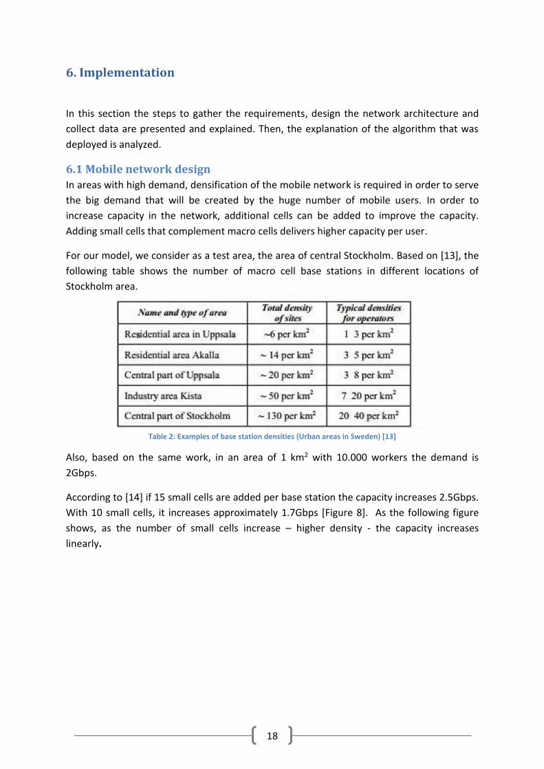
For our model, we consider as a test area, the area of central Stockholm. Based on [13], the

following table shows the number of macro cell base stations in different locations of

Stockholm area.

Table 2: Examples of base station densities (Urban areas in Sweden) [13]

Also, based on the same work, in an area of 1 km2 with 10.000 workers the demand is

2Gbps.

According to [14] if 15 small cells are added per base station the capacity increases 2.5Gbps.

With 10 small cells, it increases approximately 1.7Gbps [Figure 8]. As the following figure

shows, as the number of small cells increase – higher density - the capacity increases

linearly.

19

Figure 8: Capacity contribution of small cells and Wi-Fi as the density of small cells increases [14]

Also, as it is mentioned in Nokia’s report [30], “a typical TCO break-even may be achievable

with anything from 4-6 small cell sites per macro site (3-6 sectors) to even 10-12 for certain

street level deployments”.

In addition, in [15], an analysis of an ultra-dense mobile network is presented. In their

system, the model that is used includes outdoor small cells placed in hexagonal grid. Using

distance of 50 meter, 462 small cells are needed to cover an ultra-dense area of one square

kilometer.

Combining all the above and the assumption in [2], it is safe to consider as an optimal

scenario a system that uses 10 small cell stations attached to each base station in order to

cover an ultra-dense area.

Maps of interested with locations of Macro Cell station and identification of each area

In the images below, two different areas of Stockholm are presented. In the first image, the

Stockholm’s city center is shown, while in the secont, the area of Kista.

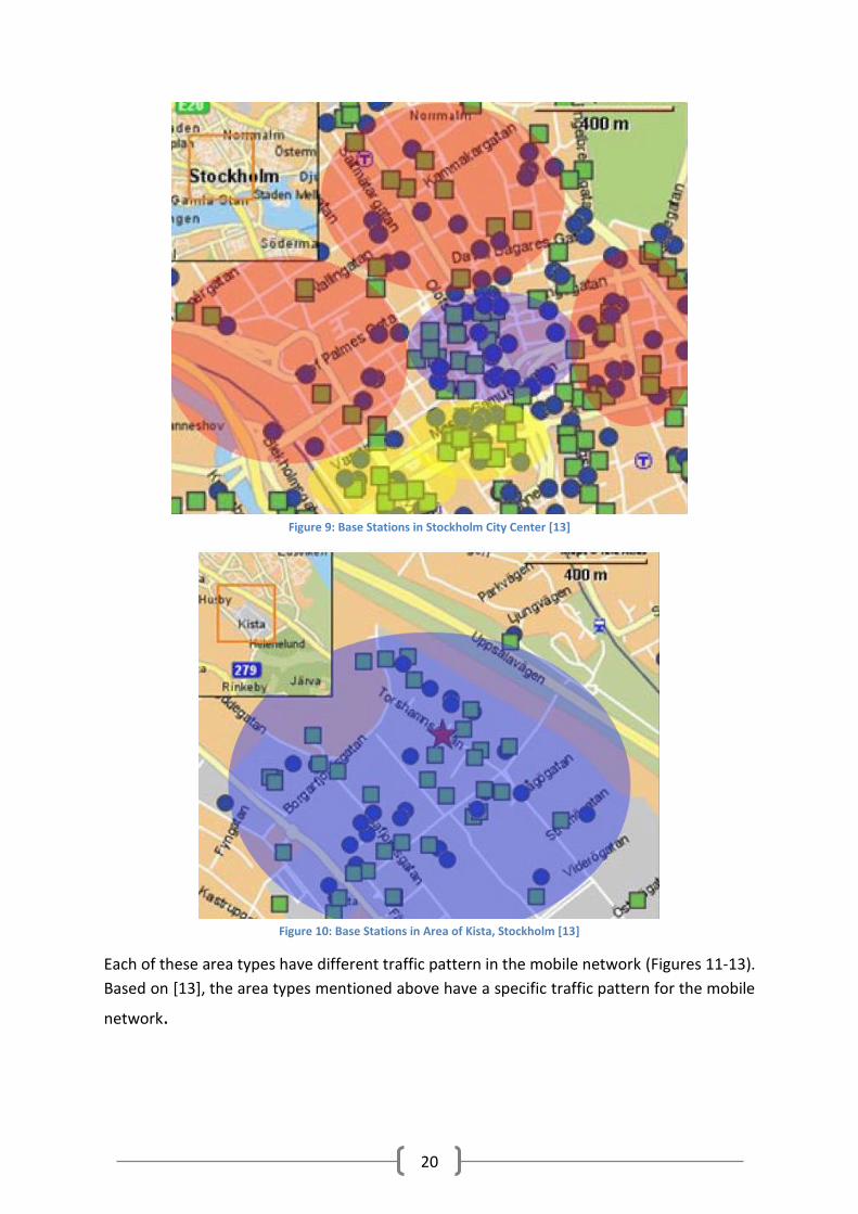
In both maps, different urban functional areas are labeled. In red, the residential area, in

blue the office area and in yellow transportation area. It is important to mention that the

selection is based on the knowledge of the areas. In advance, the circles represent GSM

towers while the squares 3G towers. In our scenario we make the assumption that those

towers will be reused for the upcoming 5G technology as it is hard and expensive to install

new towers specifically for the 5G network.

20

Figure 9: Base Stations in Stockholm City Center [13]

Figure 10: Base Stations in Area of Kista, Stockholm [13]

Each of these area types have different traffic pattern in the mobile network (Figures 11-13).

Based on [13], the area types mentioned above have a specific traffic pattern for the mobile

network.

21

Figure 11: Traffic pattern in Office area [31]

Figure 12: Traffic pattern in Resident area [31]

Figure 13: Traffic pattern in Transport area [31]

In order to identify the number of active cells in each area of interest, we need to take a

look in the normalized traffic pattern given in [31]. In the following images, the combination

of traffic patterns is showed.

22

Figure 14: Combination of normalized traffic on weekdays for Office/Transport areas [31]

Figure 15: Combination of normalized traffic on weekends for Office/Transport areas [31]

Figure 16: Combination of normalized traffic on weekdays for Resident/Transport areas [31]

Figure 17: Combination of normalized traffic on weekends for Resident/Transport areas [31]

23

In the above pictures we see a comparison of the traffic. From those pictures we can make

some assumptions about the number of active cells needed in each period of time.

Looking in the first picture, we can make the following assumptions for the number of small

cells needed for an office area:

Full capacity is required between 10:00 and 16:00. That means that all the connected small

cells in each base station need to be active. In our scenario and according to the conclusion

from the previous section, 10 out of 10 small cells are required. At 20:00 the demand drops

to 50% so we can assume that 50% of cells are needed, a number of 5 out of 10, while at

24:00, only the ¼ is needed.

During the weekend, the max number of cells needed is 50%, so the max number of small

cells we need is 5 cells per macro station.

For the transport area, during weekdays, the full capacity is needed at 08:00 and around

18:00 while between 08:00 and 16:00 only the half of the capacity is needed. For the

weekend the traffic pattern is similar to the office area demand.

Similarly, we notice that for the residential area, at 8:00 only the half of the capacity is

required, between 10:00 and 16:00 the ¾ are required while the pick is at 20:00 where the

full number of station is required. During the weekend, the traffic pattern is different, as

usually people spent time at home and they don’t work. The peak is again between 20:00

and 24:00, while between 08:00-20:00, the required capacity is more than the 3/4.

What we can observe is that, e.g. at 08:00 areas with transport characteristics need full

capacity while the office and residential areas need only the half of it. The traffic pattern

between office and transport areas is inversely proportional between the time periods of

08:00 – 16:00. Also after 20:00 where the residential area requires the peak capacity, the

office and transport area demand is decreasing. Also during the weekend, the requirements

of traffic in transport and office areas are the half of a weekday while the demand in a

residential area is in the max value.

In the following sections, a more detailed analysis is presented.

6.2 Transport Network

For each transport network architecture that was presented in the previous sections, we will

consider three different cases. In the first case, all ports from the transport network

equipment will be occupied by cells operating in the same urban area, e.g. office area. The

second scenario will involve the combination of cells operating in different areas, office-

residential, office-transport and residential-transport. The third scenario examines the case

where all the three areas, equally shared resources in each network device. The main

purpose of this analysis is to examine if we can save wavelengths by dynamically re-

assigning them to different areas.

24

6.3 Data Collection

In the following images, the combination of the normalized traffic that is shown before is

presented in one figure for weekdays and weekends respectively.

Figure 18: Summarization of traffic pattern – weekday

Figure 19: Summarization of traffic pattern – weekend

From those images, we derive the numbers and the percentage of the cells that are required

in order to serve the demanded capacity based on the traffic pattern. The three cases that

are mentioned in Section 6.2 are analyzed in order to collect valuable data.

Case 1:

Full access to:

• Office: no reuse of wavelength as the base stations need simultaneously full capacity

to serve the demand.

• Transport: no reuse of wavelength as the base stations need simultaneously full

capacity to serve the demand.

• Resident: no reuse of wavelength as the base stations need simultaneously full

capacity to serve the demand.

25

Case 2:

In the case of sharing resources between 2 different areas, each area (e.g. office and

transport) consumes 50% of the resources. So in the corresponding graph (Figure 14), the

office occupies 50% of the resources and available wavelengths. In the given example of

figure 14, the office area max capacity is 50% of the overall available network capacity as

the network resources and wavelengths are split equally between the areas. Reading the

graph, e.g. in Figure 14, the normalized value “1” is the max value. However the max value

for each area is the 50% of the total capacity as it is said before. If 1 is the 50% of total

capacity, the 0.5 in the graph is the half. This means that is the half capacity of the 50%. This

is equal to 25% of total capacity. Continuing this logic, the ¼ of the graph corresponds to

12.5% of the total available capacity.

Transport – Office (50% wavelengths in transport – 50% wavelengths in office):

Weekday (Figure 14):

04:00 - 08:00: From 4:00 to 6:00 only the 10% of the capacity is used. This means

that 90% of the bandwidth is not used. From 6:00 to 8:00, transport uses all the

available resources (50% in total) as it peaks at 8. In the same time, at 08:00 office

area uses 50% of resources (25% of total available bandwidth). If we sum the used

resources, we need resources to give us 75% of total bandwidth at 8:00. So we can

save 25% of the office area. In the case e.g. NG-PON2, the cells belonging in office

area, will demand 50% of capacity at 08:00. So from the 8 allocated wavelengths to

office areas, the 4 wavelengths are not used. The 4 wavelengths are the 25% of total

16 wavelengths.

08:00 –16:00: The traffic patterns between the two areas of interest are inversely

proportional to each other. Specifically, at 09:00, both patterns are about in ¾ of the

traffic. This means that around 25% of resources are not used. This equals with

saving around 25% of resources. Taking the example of NG-PON2, 4 wavelengths are

not used again. After this point, office needs all available bandwidth, while transport

needs less than half, around 50%-60% less that the total bandwidth. As I mentioned

above, the 50% of one area, equals to 25% of total. This gives around of 25%

available resources. So again in the case of NG-PON2, 4 wavelengths are not needed

from the transport area and can be reused.

16:00 – 18:00: The traffic pattern is similar as in the previous case. This means that

saving is up to 25%

18:00 – 20:00: Transport office at this period drops to 50% while office drops below

50%, saving is total up to 30%

26

After 20:00: After 20:00 traffic decreases in both areas saving more than 50% of

resources.

Weekend (Figure 15):

During whole weekend, it is obvious that half of the capacity is required meaning

that we save 50% of the resources.

Transport – Resident (50% wavelengths in transport – 50% wavelengths in resident):


04:00 - 08:00: At this period, traffic is in low levels allowing for great savings,

however after 06:00 we notice and rapid increase to 100% at 08:00. At this period of

time we can assume that the saving is between 75% - 30%

08:00 –16:00: Between this times there is a small increase in traffic in residential

areas. In transport areas, it drops and increases again. Saving at this time approaches

25%-40%

16:00 – 18:00: At this period both traffic increase. The saving is dropping from

37.5%-10%.

18:00 – 20:00: Here the transport’s network traffic drops to half while the

residential traffic reaches almost 100%. We can assume the saving could be around

10%-25%

After 20:00: The transport traffic drops almost to 0 after some point while the

resident traffic has a peak and after this drops quickly saving more than 50%


For the transport network, traffic demand is constantly below 50% of the total

allocation. This means that minimum we save 25% of the resources. However, the

residential area’s demand is above the ¾ of the capacity.

27

Office – Resident (50% wavelengths in office – 50% wavelengths in resident):


04:00 - 08:00: At this time, the total capacity that is needed is approximately 25%

meaning that it is possible to save more than 75%.

08:00 –16:00: Office full capacity 100% wavelengths. Residential area traffic reaches

75% of capacity allowing savings up to 12% of total resources.

16:00 – 18:00: At this period of time, the traffic pattern from office area is inversely

proportional to resident area’s traffic pattern. Studying the graph, we can conclude

that savings up to 25% are possible.

18:00 – 20:00: Residential hits full demand while office drops below 50%, giving a

save of more than 25%

After 20:00: Residential hits full demand while office drops below 50%, giving a save

of more than 50%


For the office network, traffic demand is constantly below 50% of the total

allocation. This means that minimum we save 25% of the resources. However, the

residential area’s demand is above the ¾ of the capacity.

Case 3:

Resources are equally distributed in the network device between the three areas:


04:00 - 08:00: We can separate this timeframe in two smaller sections, where from

04:00 to 06:00 the traffic is below ¼ of each meaning that 75% of resources are not

in use. From 06:00 to 08:00, transport reaches max value while office and resident

are at half. We can conclude we can save up to 33%

08:00 –16:00: Between this time frame, the office demand hits the max, not allowing

any resource traffic reach max value, the transport traffic has fallen to half and

below while in the same time the traffic to residential area increases until 16:00.

From the drop of the transport traffic with combination the demand on residential

area’s increase, we can conclude we save around 33%.

16:00 – 18:00: Office and transport demand are inversely proportional. At around

18:00 office drops to 50%. From the reuse of wavelengths between office and

28

resident area we can save up to 15%. In advance, while transport is not reaching the

top value, we can see that we save around 20% by reusing or not resources.

18:00 – 20:00: As time pass and both transport and office traffic drops, we can save

up to 35%. So we can conclude that in this time 20% - 35% can be saved.

After 20:00: After this point the traffic in the two of the three areas drops allowing

saving 40% of resources and more.

Weekend (Figure 19) :

04:00 - 08:00: At this time, the traffic is low to all of the networks.

08:00 –16:00: Transport and office network usage requires half of the capacity,

meaning that at least during this time we can save 33%. Also, the resident traffic is

around the ¾ of the traffic saving extra 8%. Adding those values we can expect a

saving of 41% at this period.

16:00 – 18:00: During this period we see an increase in the residential traffic while

we see a decrease in office traffic. However, we see a peak in transport traffic

reaching the half of the demand. We can make the assumption that the saving is

approximately 40%

18:00 – 20:00: The same applies in this period, where we can consider savings

around 40%.

After 20:00: In this period we see a peak in the residential traffic, while we see drop

in the other 2 types. Starting from 40% the saving is increasing as time passes.

Summary tables

All the above considerations are summarized in the following tables:

Weekdays

CASE/TIME 04:00-08:00 08:00-16:00 16:00-18:00 18:00-20:00 After 20:00

Transport 95%-0% 0%-50% 50%-20% 20%-50% >50%

Resident 80%-50% 50%-35% 35%-10% 10%-0% 0%

Office 95%-50% 0% 25% 25%-55% >55% Table 3: Summary of savings for non-sharing infrastructure during weekdays

29

CASE/TIME 04:00-08:00 08:00-16:00 16:00-18:00 18:00-20:00 After 20:00

Transport – Office 90%-25% 25% 25% 25%-50% >50%

Transport – Resident 75% - 30% 25%-40% 37.5%-10%. 10%-25% >50%

Office – Resident >75% 12% 25% 25% >50%

Office-Resident-Transport

75%->33% 33% 20% 20%->35% >40%

Table 4: Summary of savings for sharing infrastructure during weekdays

CASE/TIME 04:00-08:00 08:00-16:00 16:00-18:00 18:00-20:00 After 20:00

Transport 100%-50% 50% 50%-60% 60% >60%

Resident 75%-50% 50%-25% 25% 25%-15% 0%

Office 95%-75% 75%-50% 55%-60% 60% >60% Table 5: Summary of savings for non-sharing infrastructure during weekends

CASE/TIME 04:00-08:00 08:00-16:00 16:00-18:00 18:00-20:00 After 20:00

Transport – Office 50% 50% 50% 50% >50% Transport - Resident >50% 30% 30% 30% 30% Office – Resident >50% 30% 30% 30% 30%

Office-Resident-Transport

80% 41% 40% 40% >40%

Table 6: Summary of savings for sharing infrastructure during weekends

6.3 Model – Algorithm

The implementation for finding the best combination for using fewer devices based on the

traffic pattern from the base stations, involves the creation of a model that calculates the

number of small cells been used at given time. There are different types of areas generating

different traffic patterns.

For M given areas, the possible combinations are:

M, M − 1, M − 2, M − 3 , … , M − (N − 2), M − (N − 1) where N = 1, …, M-2

These combinations should be compared with the benchmark topology M-N that equals to a

single connected area, therefore M-N=1. The benchmark case refers to the case where a

single area is connected to the transport network devices (WSS) and the resources –

wavelengths – are not shared between areas.

For every possible combination, the areas need to share the network resources

(wavelengths X). In each case, the number of available wavelengths per area is calculated as:

30

X

M,

X

M − 1,

X

M − 2,

X

M − 3, … ,

X

M − (N − 2),

X

M − (N − 1)

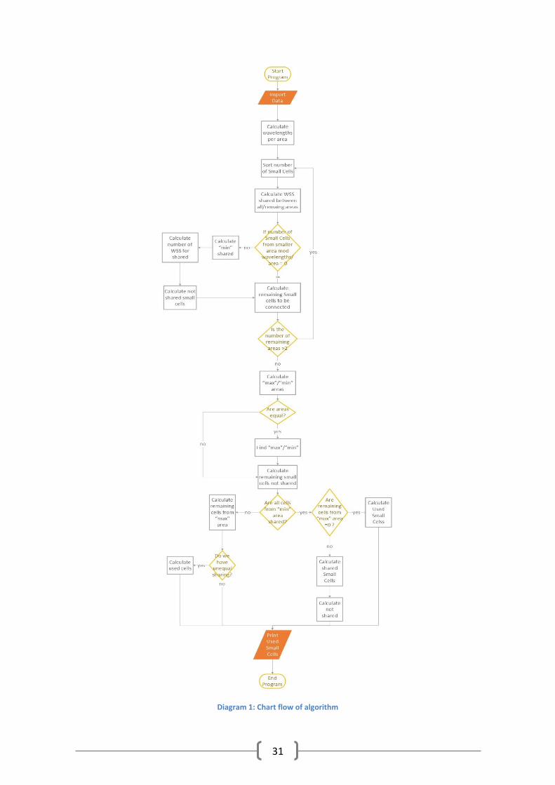
The number of small cells in every area needs to be given as input to the algorithm. The

implementation also requires the traffic percentage of the base station at given times for

the areas in question. The algorithm finds the area with the fewer small cells and calculates

how many WSSs are needed to connect those small cells.

If Sm the number of small cells in an area mϵM, then the number of WSS needed to be

shared is:

𝑆𝑚/(𝑋

𝑀)

The algorithm iterates until all the needed WSS are calculated. It also identifies if there is

equal or unequal sharing in the resources shared in a single WSS and prints the number of

the small cells required to serve the demanded traffic. The terms equal and unequal sharing

correspond to the cases where the number of small cells of different areas, connected in a

WSS, are equally or unequally distributed. The equal distribution in a WSS is represented as:

𝑆𝑚1 = 𝑆𝑚2 = ⋯ = 𝑆m−(N−1) 𝑤ℎ𝑒𝑟𝑒 𝑚 ∈ [1, 𝑀]

The algorithm continues until all the connected small cells are taken as data. Knowing the

number of the connected small cells and the percentage of the traffic, the number of the

needed small cells is calculated.

The output of the algorithm is the number of small cells required at given times during the

day and the number of the shared devices in the transport network.

The following diagram (Diagram 1) provides the flow of the algorithm.

31

Diagram 1: Chart flow of algorithm

32

6.3.1 Case Study implementation

In the following section, a detailed description about how the algorithm works and runs for

the case study of the Stockholm City Center is presented.

The implementation requires the traffic percentage of the base station at given times for

the specific areas. Also, the number of small cells for the specific areas, is calculated and

imported in the algorithm.

The algorithm takes into consideration the given transport architecture in order to calculate

how many devices can be shared in the infrastructure. This model takes as input the areas

sharing the infrastructure, the number of small cells in each area and the type of the

transport network. The output of the algorithm is the number of small cells required at

given times during the day and the number of the shared devices in the transport network.

As first step, the algorithm calculates the area with the less small cells. It divides this

number by the number of wavelengths to be shared by the transport network device. Then

it calculates the remaining number of small cells in the remaining area or areas. If the

remaining areas are two, then it calculates again the area with the fewer small cells and

calculates with the same way the number of used small cells at that time. The remaining

small cells are not sharing any infrastructure devices. However, there are cases that the

modulo of the division of small cells and wavelengths is not zero. In this case, there are

devices with unequal sharing. For example, in the case of NG-PON2, a WSS shares 16

wavelengths. If the WSS is shared among 2 areas, then each area uses 8 wavelengths. In the

case of unequal sharing, it may be the case that e.g. 3 wavelengths are used by one area and

13 for the other. In this example, the algorithm takes into consideration the shared

resources with the 6 wavelengths.

33

Diagram 2: Algorithm's chart flow for Case Study

34

More details about the algorithm’s operation are presented in the diagram (Diagram 2)

above. The program starts by prompting to import the data. If the number of shared areas

equals to three, it calculates the middle area. The terms “min”, ”middle” and “max” area

refer to the number of small cells in each area. So the “max” area is the area that has the

most small cells, the “min” area is the area with the least cells and the “middle” is the third

area. Next, it calculates the number of devices needed in order the small cells from the

“min” area to be connected and use the available resources. When all small cells from the

“min” area are connected, it calculates the remaining to be connected from the “middle”

and “max” area. Then it checks if all cells from “middle” area are connected, makes

appropriate calculations and checks if there is any unequal sharing between the areas and

prints the used small cells.

Similarly, almost the same function is performed in the case where the transport network is

shared between two areas. It calculates the “min” and “max” area and then checks if those

are equal. Then it calculates the used small cells taking under consideration the unequal

sharing, if applicable.

In the following section, the results of running the algorithm are presented. For our

scenario, we consider that the resources in the transport network are equally allocated in

the areas.

35

7. Results and Analysis

7.1 Results

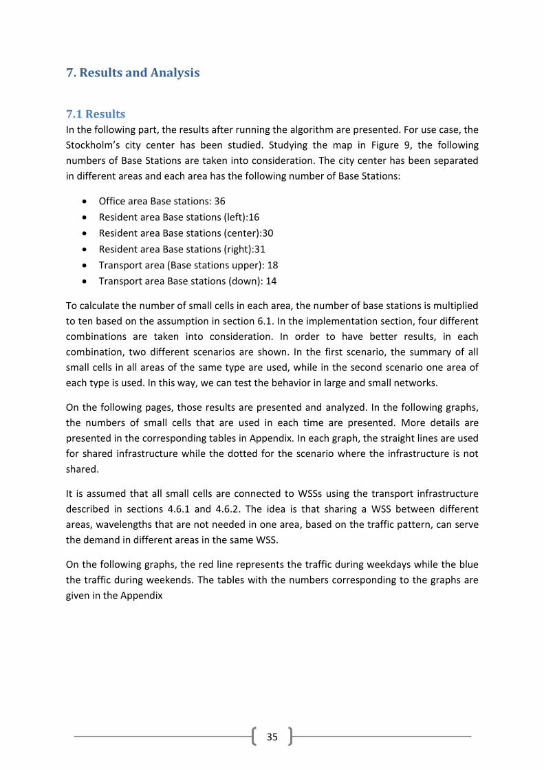
In the following part, the results after running the algorithm are presented. For use case, the

Stockholm’s city center has been studied. Studying the map in Figure 9, the following

numbers of Base Stations are taken into consideration. The city center has been separated

in different areas and each area has the following number of Base Stations:

• Office area Base stations: 36

• Resident area Base stations (left):16

• Resident area Base stations (center):30

• Resident area Base stations (right):31

• Transport area (Base stations upper): 18

• Transport area Base stations (down): 14

To calculate the number of small cells in each area, the number of base stations is multiplied

to ten based on the assumption in section 6.1. In the implementation section, four different

combinations are taken into consideration. In order to have better results, in each

combination, two different scenarios are shown. In the first scenario, the summary of all

small cells in all areas of the same type are used, while in the second scenario one area of

each type is used. In this way, we can test the behavior in large and small networks.

On the following pages, those results are presented and analyzed. In the following graphs,

the numbers of small cells that are used in each time are presented. More details are

presented in the corresponding tables in Appendix. In each graph, the straight lines are used

for shared infrastructure while the dotted for the scenario where the infrastructure is not

shared.

It is assumed that all small cells are connected to WSSs using the transport infrastructure

described in sections 4.6.1 and 4.6.2. The idea is that sharing a WSS between different

areas, wavelengths that are not needed in one area, based on the traffic pattern, can serve

the demand in different areas in the same WSS.

On the following graphs, the red line represents the traffic during weekdays while the blue

the traffic during weekends. The tables with the numbers corresponding to the graphs are

given in the Appendix

36

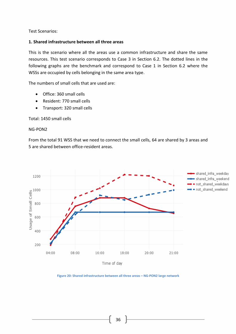
Test Scenarios:

1. Shared infrastructure between all three areas

This is the scenario where all the areas use a common infrastructure and share the same

resources. This test scenario corresponds to Case 3 in Section 6.2. The dotted lines in the

following graphs are the benchmark and correspond to Case 1 in Section 6.2 where the

WSSs are occupied by cells belonging in the same area type.

The numbers of small cells that are used are:

• Office: 360 small cells

• Resident: 770 small cells

• Transport: 320 small cells

Total: 1450 small cells

NG-PON2

From the total 91 WSS that we need to connect the small cells, 64 are shared by 3 areas and

5 are shared between office-resident areas.

Figure 20: Shared infrastructure between all three areas – NG-PON2 large network

37

WR-WDM-PON

In total, we need 48 WSS where 12 are shared by 3 areas and 1 is shared between office-

resident areas.

Figure 21: Shared infrastructure between all three areas – WR-WDM-PON large network

Analyzing the second scenario of the shared infrastructure between the three areas, smaller

network is taken under consideration:





NG-PON2

In total, we need 53 WSS to connect the small cells, where 36 are shared between 3 areas,

15 are shared between office-resident and 2 WSS assigned only to office area.

38

Figure 22: Shared infrastructure between all three areas – NG-PON2 small network

WR-WDM-PON

In total, we need 14 WSS, 6 of them are shared by 3 areas 3 are shared between office-

resident and 5 WSS assigned only to office area.

Figure 23: Shared infrastructure between all three areas – WR-WDM-PON small network

39

Observations:

In both cases, WR-WDM-PON architecture is more beneficial as fewer small cells are used

and fewer WSS are needed. The maximum number of small cells needed to serve the

demanded capacity in the case of WR-WDM-PON is smaller than the maximum number of

small cells required in NG-PON2 solution. Also, in the second scenario where smaller

networks are taken under consideration, the architecture of NG-PON2 is not optimal for the

weekends. The benchmark case, where the infrastructure is not shared requires fewer small

cells to serve the demanded capacity than the case where the infrastructure is shared.

40

2. Shared infrastructure between transport and resident areas

This is the scenario where transport and resident areas use a common infrastructure and

share the same resources. This scenario corresponds to Case 2 “transport-resident” case in

Section 6.2. The dotted lines represent the benchmark values from Case 1 in Section 6.2

where the WSS are not shared between areas.





NG-PON2

From the total 69 WSS, we need 40 WSS to be shared between transport - resident areas

and 29 to used only by resident.

Figure 24: Shared infrastructure between transport and resident areas – NG-PON2 large network

41

WR-WDM-PON

In total, we need 14 WSS where 8 WSS are shared between transport - resident areas and 6

are used only by resident.

Figure 25: Shared infrastructure between transport and resident areas – WR-WDM-PON large network

In the second scenario, the infrastructure is shared between the two areas. However, in this

case, smaller areas (in terms of small cells) are taken under consideration:




NG-PON2

For this scenario, 22 WSS are needed in total, where 20 WSS are shared between resident –

transport areas and 2 are used only by transport area.

42

Figure 26: Shared infrastructure between transport and resident areas – NG-PON2 small network

WR-WDM-PON

In total, we need to share 4 WSS between resident - transport areas and one device with

unequal sharing. The case of the unequal sharing is the scenario where the resources from

the WSS are not equally distributed among the areas. For example, if 80 wavelengths are

available in this architecture, the distribution is not equal (40 wavelengths in resident area

and 40 wavelengths in transport area).

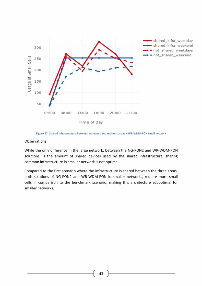
43

Figure 27: Shared infrastructure between transport and resident areas – WR-WDM-PON small network

Observations:

While the only difference in the large network, between the NG-PON2 and WR-WDM-PON

solutions, is the amount of shared devices used by the shared infrastructure, sharing

common infrastructure in smaller network is not optimal.

Compared to the first scenario where the infrastructure is shared between the three areas,

both solutions of NG-PON2 and WR-WDM-PON in smaller networks, require more small

cells in comparison to the benchmark scenario, making this architecture suboptimal for

smaller networks.

44

3. Shared infrastructure between transport and office areas

This is the scenario where transport and office areas use a common infrastructure and share

the same resources. This case corresponds to “Transport-Office” section in Case 2 of Section

6.2. Again, as in the previous scenarios, the dotted lines in the graph correspond to Case 1 in

Section 6.2. As it is stated, Case 1 is the benchmark scenario where the WSS are used only

for specific areas and are not shared.





NG-PON2

In total, we need 40 WSS to share between areas transport - office and 3 to be used only by

office area.

Figure 28: Shared infrastructure between transport and office areas – NG-PON2 large network

45

WR-WDM-PON

In total, we need to share 8 WSS between transport - office areas and 1 to used only by

office area.

Figure 29: Shared infrastructure between transport and office areas – WR-WDM-PON large network






NG-PON2

In total we need 22 WSS to be shared between transport - office areas and one WSS with

unequal sharing between the 2 areas.

46

Figure 30: Shared infrastructure between transport and office areas – NG-PON2 small network

WR-WDM-PON

In total, we need 4 WSS to be shared between areas transport - office and one WSS with

unequal sharing between those areas.

Figure 31: Shared infrastructure between transport and office areas – WR-WDM-PON small network

47

Observations:

In both cases in this scenario, sharing resources can help to reduce the number of small cells

that are used. We can observe that in both small and large networks, the benchmark case

(Case 1 – WSS are not shared between areas) requires more small cells to serve the same

capacity.

Moreover, even if it is hard to compare this scenario with the previous two scenarios

because of the different number of small cells that are taken under consideration, with the

help of Table 4 in Section 6.2, we can save up to 25% in comparison with the 20% of the

scenario where the infrastructure is shared between the three areas or transport-resident

where savings up to 10% can be achieved during weekdays.

As far as the weekends concerns for the shared infrastructure scenarios, based on Table 6 in

Section 6.2, in the “Transport-Office” areas scenario, savings up to 50% can be achieved in

comparison to “Transport-Resident” scenario where savings up to 30% can be achieved or

40% of savings in the scenario where the infrastructure is shared between the three areas.

48

4. Shared infrastructure between office and resident areas

This is the scenario where resident and office areas use a common infrastructure and share

the same resources. This scenario corresponds to Case 2 “Office-Resident” case in Section

6.2 while Case 1 from Section 6.2 is the benchmark and correspond to the dotted lines in

the figures.



• Resident:770 small cells


NG-PON2

In total, we need 45 shared WSS between areas office - resident and 26 to used only by

resident area

Figure 32: Shared infrastructure between office and resident areas – NG-PON2 large network

49

WR-WDM-PON

In total, we need 9 WSS to be shared between areas office - resident and 6 to used only by

resident area.

Figure33: Shared infrastructure between office and resident areas – WR-WDM-PON large network



• Office:360 small cells



50

NG-PON2

Figure34: Shared infrastructure between office and resident areas – NG-PON2 small network

WR-WDM-PON

Figure35: Shared infrastructure between office and resident areas – WR-WDM-PON small network

51

Observations:

In this scenario, sharing infrastructure among a large number of small cells, can reduce the

number of active cells, as fewer are needed to serve the traffic demand. However, in smaller

network, the results are not the same. During weekends, the number of small cells that is

needed to serve the demanded capacity is less in the benchmark scenario than the number

of small cells needed in the shared infrastructure.

Moreover, even if it is hard to compare this scenario with the previous three scenarios

because of the different number of small cells that are taken under consideration, with the

help of Table 4 in Section 6.2, we can save up to 12% in comparison with the 20% of the

scenario where the infrastructure is shared between the three areas, the transport-resident

area where savings up to 10% can be achieved or the above scenario where we can save

resources up to 25%.

To compare the resource savings during the weekends, this scenario can result savings up to

30% of the resources according to Table 6 in Section 6.2 while the highest number of saved

resources can be achieved in the scenario where the infrastructure is shared between

transport and office areas.

52

7.2 Summary of results

Summarizing the above observations, the following key-points presented:

1. In large networks, where the infrastructure is not shared, the number of used small

cells is much larger.

From all the above graphs, analyzing the first scenarios in each case where we study the

behavior of larger networks, it is noticed that less small cells are required to serve the

demanded traffic in the shared infrastructure than in the non-sharing transport network.

2. In WR-WDM-PON architecture, as it is expected, less shared devices are required in

the transport network because of the number of wavelengths that are used is

higher.

One of the differences in the two architectures that are used, NG-PON2 has 16 wavelengths

available while WR-WDM-PON has 80. Because of this big difference in the number of

wavelengths, fewer devices in the transport network are required in the transport network.

3. In smaller topologies, e.g. resident-transport, sharing infrastructure is not always the

optimal solution

Mostly during weekends, the number of small cells used in non-sharing infrastructure is

smaller than the shared infrastructure. The demand during weekends is not as high as

during weekdays. During weekdays when the demand is higher, in almost all the cases, the

shared infrastructure leads to fewer small cells to be active.

53

8. Conclusions and Future Work

In this section, the conclusions of the project are presented and recommendations and

ideas for future work are suggested.

8.1 Conclusions

In general, this work contributes to find a solution in sharing resources in optical transport

networks. This will lead in saving resources. A model for the calculation is built and results

are presented.

It is observed that in bigger networks with higher traffic demands, sharing infrastructure

among areas and different traffic patterns can result in bigger saving of resources.

Considering the summary tables in section 6, we calculate the percentage of the

wavelengths that are not used in given times. Considering that each wavelength

corresponds to a connected small cell, it concludes that extra small cells can be served by

the transport network. The smaller percentage from the saved wavelengths corresponds to

the percentage of the extra small cells that can be additionally served by the transport

network. To clear things up, we can consider the following example. Considering the case of

WR-WDM-PON and calculating that we can save 25% of the wavelengths, this percentage

equals to 20 out of 80 wavelengths. This means that extra 20 small cells can be served by

rerouting the wavelengths.

Another conclusion is that more saving can be achieved by turning off the small cells that

are not in use. The introduced algorithm has presented the number of cells that are

required at each time so easily can derive the number of cells that are not used in each

topology.

8.2 Future Work

This is the initial work to study if sharing resources in the transport network can be

beneficial and lead in saving more resources in terms of wavelengths and small cells. For the

scenarios where the fewer resources are used, a financial analysis can be studied to

determine the amount of money that can be saved as well.

Additionally, another model can be studied where the allocation of resources is analog to

the total number of small cells. More specifically, in this project, the allocation of resources

has been calculated and distributed equally. In the case that the resources were shared

between 2 areas, 50% of the resources were distributed in each area. However, in another

scenario, the distribution can be calculated as following. Considering the example of sharing

54

resources between 3 areas and each area has 300,600 and 900 small cells. Then the

allocation of resources will be 17%, 33% and 50% respectively. Theoretically, source sharing

will be distributed in more devices and can result to more saving.

55

References 1. Ericsson mobility report, November 2015, [Online] Available:

http://www.ericsson.com/res/docs/2015/mobility-report/ericsson-mobility-report-nov-

2015.pdf

2. COMBO Deliverable D3.3“Analysis of transport network architecture for structural

convergence”, June 2015

3. Anna Pizzinat et al., Things you should know about fronthaul, IEEE/OSA Journal of

Lightwave Technology, Volume 33, Issue 5, 2015

4. J. Homa and K. Bala. Roadm architectures and their enabling wss technology. IEEE

Communications Magazine, 46(7):150–154, July 2008

5. A. Viglienzoni, R. M. Dorward, “Evolution of Switching Technology in DWDM Networks”,

IEEE, 2009

6. N. Carapellese, M. Tornatore, and A. Pattavina, “Placement of base-band units (BBUs)

over fixed/mobile converged multi-stage WDM-PONs,” in Proc. 17th Int. Conf. ONDM, Apr.

2013, pp. 246–251

7. N. Carapellese, M. Tornatore, A. Pattavina, Energy-Efficient Baseband Unit Placement in a

Fixed/Mobile Converged WDM Aggregation Network, IEEE Journal on Selected Areas in

Communications, Aug. 2014, Vol.32(8), pp.1542-1551

8. C. Lange, A. Gladisch, “On the energy consumption of FTTH access networks,” in Proc.

Conf. OFC—Incudes Post Deadline Papers, Mar. 2009, pp. 1–3

9. R. Wang, H. H. Lee, S. S. Lee, and B. Mukherjee, “Energy saving via dynamic wavelength

sharing in WDM-PON,” in Proc. 17th Int. Conf. ONDM, Apr. 2013, pp. 235–239

10. I. L. C. Araujo, A. Klautau, “Traffic-aware sleep mode algorithm for 5G networks”

Telecommunications (IWT), IEEE Conference Publications, 14-17 June 2015

11. P. Vetter, “Next Generation Optical Access Technologies,” in European Conference and

Exhibition on Optical Communication. Optical Society of America, 2012

12. A. Banerjee, Y. Park, F. Clarke, H. Song, S. Yang, G. Kramer, K. Kim, and B. Mukherjee,

“Wavelength-Division-Multiplexed Passive Optical Network (WDM-PON) Technologies for

Broadband A”

13. Markendahl J., Mäkitalo Ö., “A comparative study of deployment options, capacity and

cost structure for macrocellular and femtocell networks”, Wireless@KTH, Royal Institute of

Technology Stockholm, Sweden

http://www.ericsson.com/res/docs/2015/mobility-report/ericsson-mobility-report-nov-2015.pdf

http://www.ericsson.com/res/docs/2015/mobility-report/ericsson-mobility-report-nov-2015.pdf

56

14. senzafiliconsulting.com [available on April 13,2016]

http://www.senzafiliconsulting.com/Portals/0/docs/Reports/SenzaFili_SmallCellWiFiTCO.pd

f

15. D. López-Pérez, M. Ding, H. Claussen and A. Jarafi, "Towards 1Gbps/UE in cellular

systems: Understanding Ultra-Dense Small Cell Deployments," in IEEE Communications

Surveys and Tutorials, vol. 17, no 4, Page(s):2078- 2101, Jun., 2015.

16. M. Nahas, A. Saadani, J. Charles, and Z. El-Bazzal, “Base stations evolution: Toward 4G

technology,” in Proc. 19th ICT, Apr. 2012, pp. 1–6.

17. A. Saadani et al., “Digital radio over fiber for LTE-advanced: Opportunities and

challenges,” in Proc. 17th Int. Conf. ONDM, Apr. 2013, pp. 194–199.

18. Seyringer, D, (2012). Design, Simulation and Evaluation of AWG Based Demultiplexers. In

The Ninth International Conference on Advanced Semiconductor Devices and Microsystems.

Smolenice, Slovakia, November 11–15. 303-306

19. Ericsson mobility report. June 2014. [Online] Available:

http://www.ericsson.com/res/docs/2014/ericsson-mobility-report-june-2014.pdf

20. NetManias Tech-Blog, Fronthaul Size: Calculation of maximum distance between RRH

and BBU, Apr 2014, available online:

http://www.netmanias.com/en/?m=view&id=blog&no=6276

21. www.cpri.info “Common Public Radio Interface; Interface Specification V6.0”

22. http://www.obsai.com/

23. Öhlen, P, 2016.” Data Plane and Control Architecture for 5G Transport Networks”.

Journal of Lightwave Technology, 34

24. 40-Gigabit-capable passive optical networks (NG-PON2): General requirements,

Recommendation ITU-T G.989.1, 2013

25. S. Gosselin et al. “Fixed and Mobile Convergence: Which Role for Optical Networks?”,

Optical Fiber Communication Conference 2015, 22–26 March 2015, Los Angeles, California

United States

26. 40-Gigabit-capable passive optical networks (NG-PON2): Physical media dependent

(PMD) layer specification, Recommendation ITU-T G.989.2, 2013

27. OASE Deliverable 4.2.1 “Technical Assessment and Comparison of Next-Generation

Optical Access System Concepts”, October 2011

28. COMBO Deliverable D6.2 “Detailed Description of COMBO Demonstration”, August 2015

http://www.senzafiliconsulting.com/Portals/0/docs/Reports/SenzaFili_SmallCellWiFiTCO.pdf

http://www.senzafiliconsulting.com/Portals/0/docs/Reports/SenzaFili_SmallCellWiFiTCO.pdf

http://www.ericsson.com/res/docs/2014/ericsson-mobility-report-june-2014.pdf

http://www.netmanias.com/en/?m=view&id=blog&no=6276

http://www.cpri.info/

http://www.obsai.com/

57

29. A. Håkansson, Portal of Research Methods and Methodologies for Research Projects and

Degree Projects. WORLDCOMP'13 - The 2013 World Congress in Computer Science,

Computer Engineering, and Applied Computing, 22-25 July, 2013 Las Vegas, Nevada; USA

30. NOKIA outdoor 3glte small cells deployment strategy whitepaper [available on 13 April

2016]

31. Wang, Huandong, Xu, Fengli ; Li, Yong ; Zhang, Pengyu ; Jin, Depeng “Understanding

Mobile Traffic Patterns of Large Scale Cellular Towers in Urban Environment” IMC '15

Proceedings of the 2015 ACM Conference on Internet Measurement Conference, Pages 225-

238

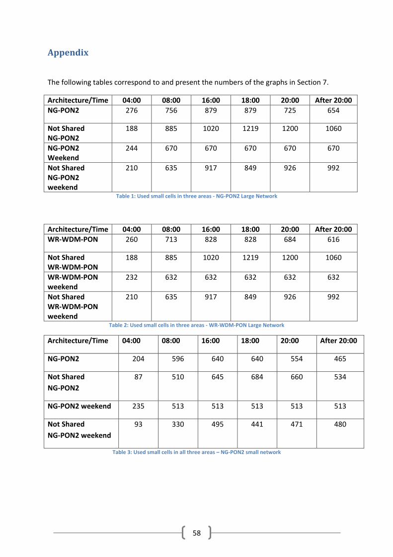
58

Appendix

The following tables correspond to and present the numbers of the graphs in Section 7.

Architecture/Time 04:00 08:00 16:00 18:00 20:00 After 20:00

NG-PON2 276 756 879 879 725 654

Not Shared NG-PON2

188 885 1020 1219 1200 1060

NG-PON2 Weekend

244 670 670 670 670 670

Not Shared NG-PON2 weekend

210 635 917 849 926 992

Table 1: Used small cells in three areas - NG-PON2 Large Network


WR-WDM-PON 260 713 828 828 684 616

Not Shared WR-WDM-PON

188 885 1020 1219 1200 1060

WR-WDM-PON weekend

232 632 632 632 632 632

Not Shared WR-WDM-PON weekend

210 635 917 849 926 992

Table 2: Used small cells in three areas - WR-WDM-PON Large Network


NG-PON2 204 596 640 640 554 465

Not Shared

NG-PON2

87 510 645 684 660 534

NG-PON2 weekend 235 513 513 513 513 513

Not Shared

NG-PON2 weekend

93 330 495 441 471 480

Table 3: Used small cells in all three areas – NG-PON2 small network

59


WR-WDM-PON 180 532 564 564 492 408

Not Shared

WR-WDM-PON

87 510 645 684 660 534

WR-WDM-PON

weekend

216 456 456 456 456 456

Not Shared

WR-WDM-PON

weekend

93 330 495 441 471 480

Table 4: Used small cells in all three areas – WR-WDM-PON small network


NG-PON2 160 480 384 576 480 320

Not Shared

NG-PON2

170 705 660 949 930 898

NG-PON2

weekend

76 448 448 448 448 448

Not Shared

NG-PON2

weekend

192 545 737 705 782 866

Table 5: Used small cells in transport and resident areas – NG-PON2 large network


WR-WDM-PON 160 480 384 576 480 320

Not Shared

WR-WDM-PON

170 705 660 949 930 898

WR-WDM-PON

weekend

76 448 448 448 448 448

Not Shared

WR-WDM-PON

weekend

192 545 737 705 782 866

Table 6: Used small cells in transport and resident areas – WR-WDM-PON large network

60


NG-PON2 80 240 192 288 240 160

Not Shared

NG-PON2

41 260 194 288 250 232

NG-PON2

weekend

38 224 224 224 224 224

Not Shared

NG-PON2

weekend

40 170 210 192 208 214

Table7: Used small cells in transport and resident areas – NG-PON2 small network


WR-WDM-PON 90 270 216 234 270 180

Not Shared

WR-WDM-PON

41 260 194 288 250 232

WR-WDM-PON

weekend

42 252 252 252 252 252

Not Shared WR-

WDM-PON weekend

40 170 210 192 208 214

Table 8: Used small cells in transport and resident areas – WR-WDM-PON small network


NG-PON2 64 480 480 480 320 256

Not Shared

NG-PON2

34 500 520 526 430 290

NG-PON2

weekend

32 320 320 320 320 256

Not Shared

NG-PON2

weekend

18 250 340 272 272 222

Table 9: Used small cells in transport and office areas – NG-PON2 large network

61


WR-WDM-PON 64 480 480 480 320 256

Not Shared

WR-WDM-PON

34 500 520 526 430 290

WR-WDM-PON

weekend

32 320 320 320 320 256

Not Shared

WR-WDM-PON

weekend

18 250 340 272 272 222

Table 10: Used small cells in transport and office areas – WR-WDM-PON large network


NG-PON2 36 273 273 273 182 144

Not Shared

NG-PON2

27 360 450 414 360 234

NG-PON2

weekend

17 182 182 182 182 144

Not Shared

NG-PON2

weekend

18 180 270 216 216 180

Table 11: Used small cells in transport and office areas – NG-PON2 small network


WR-WDM-PON 38 285 285 285 190 152

Not Shared

WR-WDM-PON

27 360 450 414 360 234

WR-WDM-PON

weekend

19 190 190 190 190 152

Not Shared WR-WDM-

PON weekend

18 180 270 216 216 180

Table 12: Used small cells in transport and office areas – WR-WDM-PON small network

62


NG-PON2 180 633 540 540 540 360

Not Shared

NG-PON2

172 565 860 963 1040 932

NG-PON2

weekend

108 503 503 503 503 503

Not Shared

NG-PON2

weekend

210 475 757 721 798 896

Table 13: Used small cells in office and resident areas – NG-PON2 large network


WR-WDM-PON 180 633 540 540 540 360

Not Shared

WR-WDM-PON

172 565 860 963 1040 932

WR-WDM-PON

weekend

108 503 503 503 503 503

Not Shared

WR-WDM-PON

weekend

210 475 757 721 798 896

Table 14: Used small cells in office and resident areas – WR-WDM-PON large network


NG-PON2 150 527 450 450 450 300

Not Shared

NG-PON2

78 330 555 540 570 462

NG-PON2

weekend

89 419 419 419 419 419

Not Shared

NG-PON2

weekend

93 240 405 369 399 426

Table 15: Used small cells in office and resident areas – NG-PON2 small network

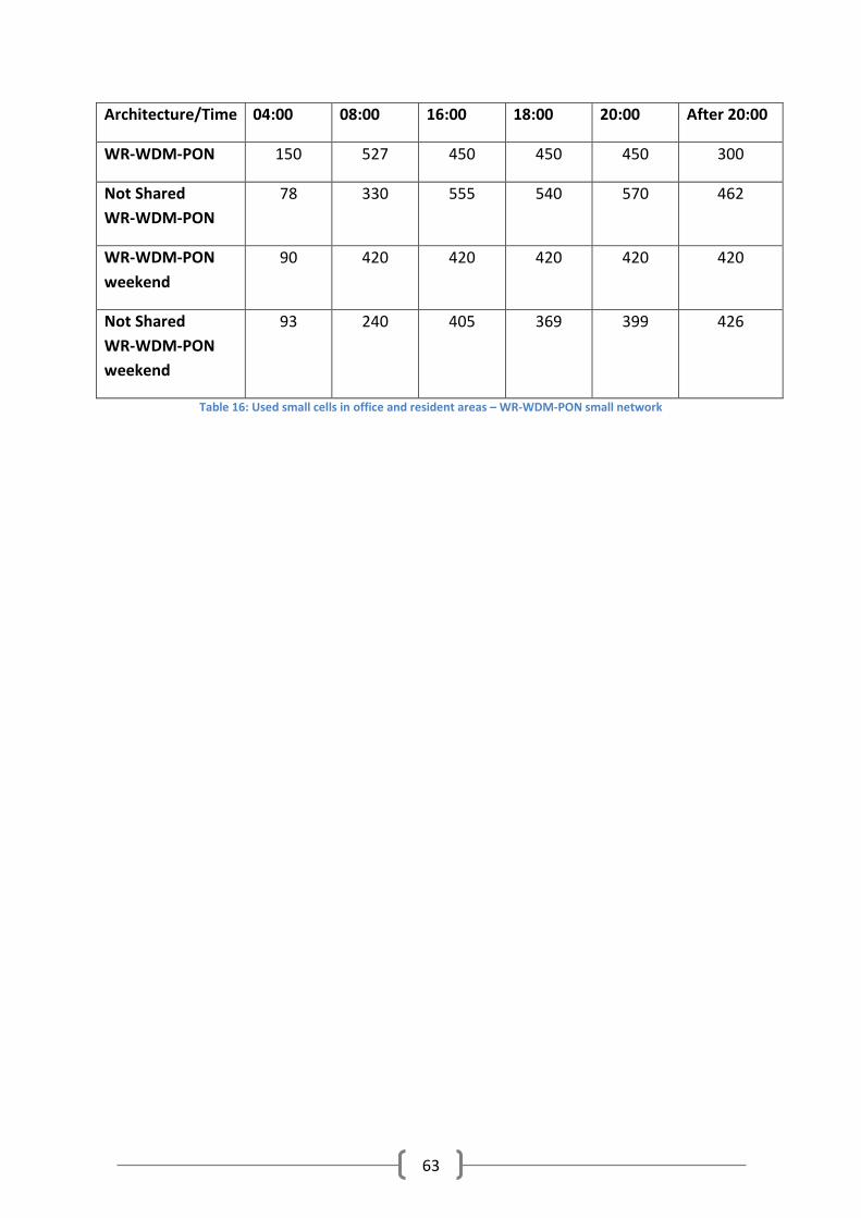
63


WR-WDM-PON 150 527 450 450 450 300

Not Shared

WR-WDM-PON

78 330 555 540 570 462

WR-WDM-PON

weekend

90 420 420 420 420 420

Not Shared

WR-WDM-PON

weekend

93 240 405 369 399 426

Table 16: Used small cells in office and resident areas – WR-WDM-PON small network

TRITA ICT-EX-2017:26

www.kth.se

Documents

Dynamic Optical Resource Allocation in Transport Networks ...kth.diva-portal.org/smash/get/diva2:1096090/FULLTEXT01.pdf · i Abstract Mobile traffic increases rapidly. Based on Ericsson’s