Dynamic Modeling and Simulation of Flexible Beam Finite

715

ISSN 1392−1207. MECHANIKA. 2018 Volume 24(5): 715−724

Dynamic Modeling and Simulation of Flexible Beam Finite Rotation

with ANCF Method and FFR Method

Ling HAN*, Ying LIU**, Bin YANG***, Yueqin ZHANG**** *Nanjing Forestry University, Nanjing 210037, China, E-mail: [email protected]

**Nanjing Forestry University, Nanjing 210037, China, E-mail: [email protected]

***Nanjing Institute of Technology, Nanjing, 211167, China, Email: [email protected]

****Nanjing University of Aeronautics and Astronautics, Nanjing, 210016, E-mail: [email protected]

http://dx.doi.org/10.5755/j01.mech.24.5.20358

1. Introduction

The earliest method discovered for dealing with

flexible body dynamic equations is the kineto-elasto-dy-

namic (KED) method [1–3]. This method is based on as-

sumptions of low speed and small displacement, while the

coupling terms of rigid-body motion and elastic motion in

the dynamic equations are neglected. The inertia character-

istics of flexible body rigid motion are loaded onto the flex-

ible body itself in the form of inertial forces. With the con-

stant emergence of lightweight, high-speed machinery, the

disadvantages of the KED method have been gradually ex-

posed [4]. To describe the effect of elastic deformation of

the flexible body on its own large overall motion, Likins [5]

proposed the floating frame of reference (FFR). The FFR

method decomposes the configuration of the flexible body

into two parts: the large overall rigid motions of the floating

coordinate system, and the elastic deformation of the flexi-

ble body with respect to the floating coordinate system. Alt-

hough the selection of the floating coordinate system does

not affect the analysis results, the mass matrix obtained by

this method is a nonlinear function matrix of generalized co-

ordinates, resulting in inertial coupling between the rigid

motion and elastic deformation of the flexible body.

To simplify the mass matrix, Simo [6–9] suggested

suppressing the floating coordinate system and expressing

the beam's dynamic equations in the global coordinate sys-

tem directly. In describing the bending and shearing of the

beam, Simo reserved the beam's cross-section local coordi-

nate system containing the cross-section angle relative to the

beam rigid configuration. Simo's approach simplifies the ex-

pression of the kinetic energy of the beam compared to the

FFR method. The constant mass matrix can be obtained us-

ing variable separation; however, the expressions of elastic

potential energy and the stiffness matrix become more com-

plex.

At the end of the 20th century, Shabana and other

scholars [10–14] proposed the absolute nodal coordinate

formulation (ANCF) method. This method is similar to that

proposed by Simo: the dynamic equations of the beam are

described in the global coordinate system; the cross-section

local coordinate system of the beam is used to describe

bending, shearing, and twisting; and the constant mass ma-

trix can be obtained, so the centrifugal force and Coriolis

force are zero. The shortcomings of these two methods are

identical: the stiffness matrix becomes highly complicated.

In contrast to Simo's method, in the ANCF ap-

proach, the cross-section slopes at the nodes (instead of the

cross-section angles) become the beam's generalized coor-

dinates. Therefore, the rigid-body inertia of the beam can be

described accurately, and the constant mass matrix can be

obtained without needing to perform variable separation on

generalized coordinates.

For the flexible body dynamic simulation, however,

a simple mass matrix and simple stiffness matrix cannot be

obtained simultaneously. The stiffness matrix obtained with

the FFR method is relatively simple, but the mass matrix is

a nonlinear function matrix of the generalized coordinates.

If the floating coordinate system is suppressed and the dy-

namic equations are expressed in the absolute coordinate

system, then the mass matrix can be reduced to a constant

matrix, but the stiffness matrix becomes highly nonlinear.

In this paper, based on assumptions of low speed

and small deformation, the ANCF method is considered a

finite element interpolation method. The interpolation ma-

trices, mass matrix, and stiffness matrix of the two-node

beam element are extended to those of the multi-node beam

element, thereby improving calculation accuracy. The

ANCF method is combined with the FFR method (for con-

venience, the combination of these two methods is termed

the ANCF-FFR method). The stiffness matrix, which does

not include generalized coordinates, is obtained along with

the constant mass matrix. In the ANCF method, the bending

moment is a nonlinear function vector of the generalized co-

ordinates, so it is difficult to solve the system states directly.

The split-iteration method is used to solve the system states

and Lagrange multipliers. This algorithm guarantees a suf-

ficiently accurate solution and improves the computational

efficiency substantially.

2. Modeling and solving methods for flexible beam

finite rotation

To improve simulation accuracy, the expressions

of the generalized coordinates, interpolation matrices, mass

matrix, stiffness matrix, and generalized forces of the two-

node beam are extended to those of the multi-node beam.

The FFR method is combined with the ANCF method to ob-

tain the stiffness matrix, which does not contain the gener-

alized coordinates. To enhance the efficiency of the simula-

tion, the splitting iteration method is used to solve both the

static and dynamic equations.

2.1. Generalized coordinates, interpolation matrix, and mass

matrix

Fig. 1 displays the schematic diagram of the global

coordinate system and the local coordinate system based on

mailto:[email protected]

http://dx.doi.org/10.5755/j01.mech.24.5.20358

716

the ANCF method. For convenience, the number of nodes

on the neutral axis of the beam is set to 4. The global coor-

dinate system is (O, r1, r2, r3), and the local coordinate sys-

tem is (A1, x, y, z). The original point of the local coordinate

system is located at the beam's neutral axis endpoint, A1; the

coordinate x is the arc length coordinate of the beam neutral

axis; A1y is the axis along the height direction of the beam

cross-section; and A1z is the axis along the width direction of the beam cross-section.

Fig. 1 The coordinate systems of the ANCF method

Let the mass density of the rectangular beam be ρ,

the height of the cross-section be h, and the width of the

cross-section be w. The four nodes on the beam's neutral

axis are A1, A2, A3, A4, which divide the beam into three ele-

ments. The length of the neutral axis of the ith element is Li

(i=1, 2, 3). The generalized coordinates of each node are

defined as:

TT T T

T

T

1 2 3

, , ,

( , , ) , 1 , 2 , , 4.

;

3

ii

i i i

AA

A A Ax y z

r r r i

=

= =

r r re r

r

(1)

The generalized coordinates of the beam can be ex-

pressed as:

1 4

T T T

48 1) ( ( , , ) .k A Ae = =e e e (2)

set

00

3

0 ;

;

,

1 , 2 , 3;

i k ik

i i

x L L

y h i

L

z w

=

= −

= =

=

=

(3)

and the scale functions are:

( )

( )

( )

( )

3 2

2 3

, , 2 3 1;

, , 2 ;

, , ;

, , .

L

xL

yL

zL

f a b c a a

f a b c a a a

f a b c b b a

f a b c c c a

= − +

= − +

= −

= −

(4)

( )

( )

( )

( )

2 3

3 2

, , 3 2

, ,

,

;

;

, ;

, , .

R

xR

yR

zR

f a b c a a

f a b c a a

f a b c b a

f a b c c a

= −

= −

=

=

(5)

The interpolation functions of the ith element are

defined as:

( )

( )

( )

( )

, , ;

, , ;

, , ;

, , ;

1 , 2 , 3.

i L i i i

i i xL i i i

i yL i i i

i zL i i i

SL f

SLx L f

SLy h f

SLz w f

i

=

=

=

=

=

(6)

( )

( )

( )

( )

1

1

1

1

, , ;

, , ;

, , ;

, , ;

1 , 2 , 3.

i R i i i

i i xR i i i

i yR i i i

i zR i i i

SR f

SRx L f

SRy h f

Rz w f

i

+

+

+

+

=

=

=

=

=

(7)

Define matrices:

3 12

3 12

1 , 2 ,

;

3;

2 , 3 , 4;

;

i i i i i

j i i i i

SL SLx SLy SLz

i

SR SRx SRy SRz

j

=

=

=

=

SL I I I I

SR I I I I (8)

where: I is the 3-order identity matrix. The interpolation ma-

trix of the beam elements between two adjacent nodes Ai,

Ai+1 can be expressed as:

1 1 2 3 12 3 12 3 48

2 3 12 2 3 3 12 3 48

3 3 12 3 12 3 4 3 48

;

;

.

=

=

=

S SL SR 0 0

S 0 SL SR 0

S 0 0 SL SR

(9)

The symbol 0 means the zero matrix, and the ele-

ments of Si (i=1, 2, 3) are the functions of x, y, z. Let P be

an arbitrary point on the beam element between nodes Ai and

Ai+1. The position vector of P in the global coordinate sys-

tem can be expressed as follows:

( , , ) ; 1 , 2 , 3.iP Px y z i ==r S e (10)

Then, the kinetic energy of the beam is:

( )T 3

T

1

1 d dd ,

2 d di

i i ii V

T Vt t

=

=

e eS S (11)

and the mass matrix of the beam is:

717

( )3

T

1

d ,

i

i i ii V

V=

=M S S (12)

where: M is a symmetric positive definite constant

matrix.

2.2. Strain energy and stiffness matrix

The generalized displacement produced by elastic

deformation at point P on the ith (i=1, 2, 3) beam element

can be expressed as:

( ) ( )0 , , ;

1 , 2 , 3.

iP Px y z

i

= −

=

u S e e (13)

where: e0 is the generalized coordinate vector of the beam

in its rigid configuration. The deformation gradient of P is:

( ) ; , , ,P

P P

x y z

= = =

u u xD x

r x r (14)

where:

( )

( )

0( , , ) ;

1 , 2 , 3 ; , ,

i

P P

x y z

i x y z

= −

= =

uS e e

x x

x

(15)

Given low-speed and small-deformation assump-

tions and the FFR method, the ANCF local coordinate sys-

tem can be considered the float coordinate system in the

FFR method, i.e.,

2 2 1 1

3 3 1 1

3 3 2 2

1 0 0 0 0

0 0 1 0 0 ,

0 0 0 0 1

cos sin cos sin

cos sin sin cos

sin cos sin cos

= − − −

x

r. (16)

where: ψ1, ψ2, ψ3 represent the Caldan angles. The Cauchy

strain tensor of point P is:

( )C11 C12 C13

T

C C21 C22 C23

C31 C32 C33

1|

2P

P

P

= + =

ε D D (16)

and its vector form is:

T

CV C11 C22 C33 C12 C31 C23 , , , , , | ( 2 2 2 )P P =ε (17)

The elastic matrix Q is:

( )

( )( )( )

( )

( )

11 1

11 1

11 11

,1 21 2 1

2 1

1 2

2 1

1 2

2 1

E

− − − − − −− =

−− +

− −

− −

−

Q . (19)

where: E is the elastic modulus and μ is the Poisson's ratio.

To eliminate the Poisson locking phenomenon, we set μ=0;

thus, the elastic matrix Q can be expressed as:

( )diag / 2 / 2 / 2 .E E E E E E=Q (18)

The elastic strain energy of the ith beam element is:

T

CV CV

1d 1 , 2 , 3.

2;

iSi iV

E V i= = ε Q ε (19)

The elastic strain energy of the beam is:

3

1

.S Sii

E E=

= (20)

Based on the assumptions of low speed and small

deformation, geometric nonlinearity is ignored, and the tan-

gent stiffness matrix of the beam can be approximated as:

2

48 48

,i j

E

e e

=

K (21)

where: K is a symmetric positive semi-definite matrix that

does not include the generalized coordinates.

718

In summary, for low-speed, small-deformation

problems, we can combine the ANCF method and FFR

method to obtain the constant mass matrix and stiffness ma-

trix, which does not include the generalized coordinates.

2.3. Gravity

The virtual displacement by gravity at point P on

the element between two adjacent nodes Ai, Ai+1 is set to δe,

and then the virtual work done by gravity at point P is:

(0 , , 0)

(0 , , 0) ,

G PP

i P

W g

g

= − =

= −

r

S e

(22)

where: g denotes gravitational acceleration. From that, we

can obtain:

Td[(0 , , 0) ] ,

di P

P

gV

= − G

S (23)

where: V is the beam volume. The gravity on the beam el-

ement between Ai, Ai+1 is:

T[(0 , , 0) ] d ,i i

i iV Vg V= − G S (24)

and the overall gravity of the beam is:

3T

1

[(0 , , 0) ] d .i

i iVi

g V=

= − G S (25)

2.4. Bending moment

As shown in Fig. 2, a bending moment MB is

placed at the cross-section of point A2, its magnitude is M.

Fig. 2 The bending moment at cross-section of point A2

The virtual work of the bending moment MB is:

.B

W M = M (26)

From [15–16], the rotation angle θ of the cross-sec-

tion satisfies the following:

( ) ( )

( ) ( )

2

2 2

2

2 2

2

2 2

1 2

1

2 2

1 2

/;

/ /

/.

/ /

A

A A

A

A A

r ycos

r y r y

r ysin

r y r y

=

+

−=

+

(27)

so

20 19 19 20

2 2

19 20

,e e e e

e e

− + =

+ (28)

and the bending moment MB can be expressed as:

20

2 2

19 20

19

2 2

19 20

0 19,20

19 .

20

B

i

M ei

e e

M ei

e e

−

= =+

=

+

M (29)

2.4. Boundary conditions

Let the beam rotate anticlockwise around the Or3

axis. A constant bending moment vector MB is placed at the

cross-section of point A2. We set the boundary conditions in

the rotating process as follows:

a. At point A1, the vector

1

T

31 2 , , A

rr r

y y y

is parallel

with the vector (r1 , r2, r3)T

A1 :

1 1 8 2 7Π ( ) ( ) ( ) ( ) 0;( )e et t t tete= − (30)

b. The distance between point A1 and O(0, 0, 0) is a con-

stant:

2 2 2 2

2 1 2 3Π ( ) ( ) ( ) ( ) ;e e e Ht t t t= + + (31)

c. The coordinate r3 of point A1 is zero:

3 3Π ( ) ( 0;)et t= (32)

d. The coordinate 3r y of point A1 is zero:

4 9Π ( ) ( 0;)et t= (33)

e. Let the angle displacement function φ(t) is a known

function. The coordinate r1 of point A2 satisfies:

( )

2 2

5 13 1 2

1 2

( ) 0;

;

Π ( ) ( ) ( )t t te A A H cos

arctan H A A

= − + +

= (34)

f. The coordinate r2 of point A2 satisfies:

719

2 2

6 14 1 2Π ( ) ( ) ( ( 0) )e A A H tsint t = − + + (35)

g. The coordinate r3 of point A2 is zero.

7 15Π ( ) ( 0)et t= . (36)

Fig. 3 is the schematic diagram of finite rotation

boundary conditions of the beam.

Fig. 3 The schematic diagram of finite rotation boundary conditions of the beam

2.5. Solution of initial states

The static equilibrium equation of the system at the

moment of t=0 can be expressed as:

( )00 0 ,0 =1, ,7Π

t t

i i

= = = + + +

=

eMK e G Π λ K e (37)

where: e0 is the rigid configuration of the beam, λ is the vec-

tor of the Lagrange multipliers, and Πe is defined as:

( )48 7

Π .j ie

= eΠ (38)

For the expression of generalized force vector:

0( ) ,Gen = + + + eF e G Π λ K eM (39)

contains the nonlinear terms of the generalized coordinates

and the coupling terms between the generalized coordinates

and Lagrange multipliers, it is difficult to solve the system

states directly. The split-iteration algorithm is thus used to

solve Equation (37).

For convenience, assume the following conven-

tions: Let N1 and N2 be two sets such that:

1

1 2

1 2

1 , 2 , 3 , 9 , 13 , 14 , 15 ;

1 , 2 , 3 , 48

.

, ;

N

N N

N N

=

=

=

(40)

Set matrix A=(aij)s×t, vector v=(vk)r; A(c1,…,cn)

(b1,…,bm) is the

submatrix of A, v(d1,…,dl) is the subvector of v:

1

1

( , , )

( , , )

1 1

( ) ;

= , , ; = , , .

n

m

c c

ij m nb b

m n

a

i b b j c c

=A (41)

1( , , ) 1( ) ; = , , .ld d k l lv k d d=v (42)

Using the above agreements, we set:

( )( )

1

7

7

1 , ,

1 1, , 7; , , ;iD

D i i

ii i N= K K (43)

( )( )41

4

1

1 1

, ,

1 2, , 41; , , ;j jR

R jjj j N= K K (44)

( )( )7

41 1

1 , ,

1 1, 1 1, 7 4 2; , , , , ; ;iD

R

i

j ji i N j j N= K K (45)

( )( )41

7

1

1

, ,

1 1 1, , 7 41 2; , , , , ; ;jR

D

j

i ii i N j j N= K K (46)

( )1 7 1, 71,; , , ; D i i

i i N= e e (47)

( )1 41

411 2, ,; , , ;R j j

j j N= e e (48)

( )1 7 1 1, 7,) ;( ; , ,D Gen i i

i i N= F F (49)

( )411 41 21, ,( ; , ,) ;R Gen j j

j j N= F F (50)

720

where: KR

R and KD

D are invertible matrices. Equation (37)

can be expressed as:

;

;

0 ; =1, ,( ) 7.

R D

R R R R D

D R

D D D D R

i t i

= −

= −

K e F K e

K e F K e (51)

set

( )( )

1

3 1 2

diag , , , , 1,

R R R

R R R

p p p p

−

= − =

=

K K K

(52)

where: KR

R1 and KR

R2 satisfy:

1 2 ,R R R

R R R+ =K K K (53)

so

1 2

1 , .

1 1

R R R R

R R R R

p

p p

−= =

− −K K K K (54)

The first equation of (51) can be written as:

,1

1 1

R R D

R R R R R R D

p

p p = + −

− −K e F K e K e (55)

and we can get the iterative algorithm:

( ) ( )( ) ( )( )( )

111 ,

.

k kR D

R R R R R D

k

R

p

p

−+ = − − +

+

e K F e λ K e

e

(56)

Equation (58) is convergent when p∈[0,1). If the

elastic modulus of the material is sufficiently large, then the

fast convergence rate can be obtained when p=0.

Because the generalized force vector FR is a non-

linear function vector of eR and λ, the right side of Equation

(56) should be simplified before each iteration. For small

deformation problems, expanding the right side of (56) to

the 2nd-order Taylor series at eD=eDr, λ=0 before each itera-

tion can ensure sufficient accuracy of the solution, where eDr is:

( ) ( )( )2 22 2

1 2 1 2 , , 0 , , 0 + , + , 0 .Dr Hsin Hcos A A H cos A A H sin = − + + e (59)

Finally, eR converges to the 2nd-order Taylor series

of eD and λ.:

( , ).R R D=e e e λ (57)

After that , the constraint Eqs: (30)–(36) and the

second equation in (51) should be linearized to the 1st-order

Taylor series at eD=eDr, λ=0, and combined with Equation

(57), eR, eD and λ can be solved quickly.

2.6. Solution of dynamic equations

The dynamic equations of the beam can be ex-

pressed as:

( )2

2

d d,

.dd

0, =1 , ,7Π

Gen

i

ttt

i

+ + =

=

e eM C K e F e

(58)

Let the damping matrix C=0, and Equation (58)

can be solved with the Newmark method:

( )2 2

2 2

d d d d1 ;

d d d dt t t t t t

t tt t t t

+ +

= + − + e e e e

(59)

22

2

22

2

d 1 d

d 2 d

;d

d

t t t

t t

t t

t tt t

tt

+

+

= + + − +

+

e ee e

e

(60)

( )2

2

d, ,

dt t t t Gen t t

t t

t tt

+ + +

+

+ = +e

M K e F e (61)

where: β=0.25, γ=0.5. After rearranging Eqs. (59)–(61), we

can get:

( )

( ) ( )

2

1 2

2

1 2 2

2

, ;

1

1

;

;

d1 ;

2 d

.

t t Gen t t

t t

Gen t t Gen

t t

t

t t

t

t t

tt t

+ +

+

+

= +

= +

= + + +

= + + −

=

K e F e

K M K

F e F F F

e e eF M

F 0

(62)

Eq. (62) can be solved using the method described

in Section 2.6.

3. Numerical example

Set the length of the rectangular section beam as

7.791m. The position of each node on the beam is shown in

Figure 3.the width of the cross-section as w=0.1m, the

height of the cross-section as h=0.1m, the elastic modulus

as E=2.1×1011Pa, the mass density as ρ=7850kg/m3, and Poisson's ratio as μ=0.3. The boundary conditions are de-

scribed in Section 2.5, and OA1 satisfies the following:

1 0.295m.OA H = (63)

The lump mass m is fixed at the endpoint of the

721

beam. The constant bending moment MB is loaded at the

cross-section of node A2, and:

1000Nm.B =M (64)

The beam angular displacement functionφ(t) satis-

fies:

1

0 0

( ) 0.1 rad s ) 0 5s.

0 5s

(

t

t t t

t

−

=

(65)

Figs. 4 and 5 denote the static deflection of the end-

point of the neutral axis of the beam obtained by the ANCF-

FFR method and ABAQUS simulation when the lump mass

m = 0 kg and m = 50 kg, respectively. The angles between

the beam rigid configuration and the Or1 axis are set at 0

degrees, 15 degrees, 30 degrees, 45 degrees, 60 degrees, re-

spectively. When using the ANCF-FFR method, the num-

bers of nodes on the neutral axis of the beam are 4, 10, 16,

22, and 28, respectively. In the ABAQUS software, the

beam model is divided into 4192 2nd-order hexahedral ele-

ments. The charts and tables indicate that when the number

of nodes on the neutral axis of the beam is small, the results

obtained by the ANCF-FFR are quite different than those in

the ABAQUS simulation. As the number of nodes increases,

the ANCF-FFR results tend to be consistent with those of

ABAQUS. When the number of nodes in ANCF reaches 28,

the relative error of the two methods is less than 1%, a sat-

isfactorily accurate proportion for engineering machin-

ery such as cranes and aerial work platforms.

0 15 30 45 60

-36

-33

-30

-27

-24

-21

-18

-15

-12

-9

-6

En

d p

oin

t sta

tic e

lastic d

ispla

ce

me

nt(

mm

)

Angle(degree)

ABAQUS results

ANCF-FFR results(4 nodes)





Fig. 4 The endpoint static deflections when m=0kg

0 15 30 45 60

-50

-45

-40

-35

-30

-25

-20

-15

-10

-5

En

d p

oin

t sta

tic e

lastic d

ispla

ce

me

nt(

mm

)

Angle(degree)






ABAQUS results

Fig. 5 The endpoint static deflections when m=50 kg

0 5 10

0

1

2

3

4

Steady-state vibration after braking

Braking stage

Luffing stage

En

d p

oin

t d

yna

mic

defle

ction

(m

)

Time (s)

4 nodes results

10 nodes results

16 nodes results

22 nodes results

28 nodes results

ABAQUS resultsStarting stage

Fig. 6 The endpoint dynamic deflection (m=0 kg)

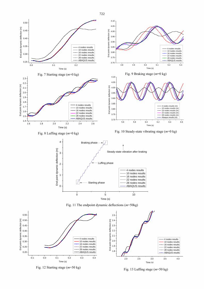
Let the initial state of the beam be the horizontal

static equilibrium state. Figs. 6 and 11 display the dynamic

deflections of the beam during the starting stage, luffing

stage, braking stage, and steady-state vibrating stage ob-

tained by the ANCF-FFR method and ABAQUS software

when the lump mass m = 0 kg and m = 50 kg, respectively.

Figs. 7–10 and Figs. 12–15 are the local charts of every

stage when m = 0 kg and m = 50 kg, respectively. From the

starting stage to the steady-state vibrating stage after brak-

ing, the results of the 4-node beam clearly deviate from

other results. The results of the 10-node beam agree well

with the ABAQUS simulation results during the starting

stage, but subsequent phase errors increase significantly

over time during the luffing stage and the steady--state vi-

brating stage. The 16-node results show good pre-braking

performance. In the steady-state vibrating stage, however,

the phase errors between the 16-node results and the

ABAQUS results are slightly larger. The 22-node and 28-

node results are almost completely aligned with the

ABAQUS simulation results. Of course, an increase in ac-

curacy requires an increase in computing time.

722

0.0 0.1 0.2

0.25

0.30

0.35

0.40

0.45

0.50E

nd p

oin

t d

yn

am

ic d

efle

ction

(m

)

Time (s)

4 nodes results

10 nodes results

16 nodes results

22 nodes results

28 nodes results

ABAQUS results

Fig. 7 Starting stage (m=0 kg)

1.6 1.8 2.0 2.2 2.4 2.6

1.4

1.5

1.6

1.7

1.8

1.9

2.0

2.1

2.2

2.3

End p

oin

t dynam

ic d

eflection (

m)

Time (s)

4 nodes results

10 nodes results

16 nodes results

22 nodes results

28 nodes results

ABAQUS results

Fig. 8 Luffing stage (m=0 kg)

4.8 4.9 5.0 5.1 5.2 5.33.70

3.75

3.80

3.85

3.90

3.95

4.00

4.05

4.10

End p

oin

t dynam

ic d

eflection (

m)

Time (s)

4 nodes results

10 nodes results

16 nodes results

22 nodes results

28 nodes results

ABAQUS results

Fig. 9 Braking stage (m=0 kg)

5.6 5.8 6.0 6.2 6.4 6.63.70

3.75

3.80

3.85

3.90

3.95

4.00

4.05

4.10

En

d p

oin

t d

yna

mic

defle

ction

(m

)

Time (s)

4 nodes results (m)

10 nodes results (m)




Abaqus results (m)

Fig. 10 Steady-state vibrating stage (m=0 kg)

0 5 10

0

1

2

3

4

Steady-state vibration after braking

Braking phase

Luffing phase

En

d p

oin

t d

yn

am

ic d

efle

ction

(m

)

Time (s)

4 nodes results

10 nodes results

16 nodes results

22 nodes results

28 nodes results

ABAQUS results

Starting phase

Fig. 11 The endpoint dynamic deflections (m=50kg)

-0.1 0.0 0.1 0.2 0.3 0.4

0.20

0.25

0.30

0.35

0.40

0.45

0.50

0.55

End p

oin

t dynam

ic d

eflection (

m)

Time (s)

4 nodes results

10 nodes results

16 nodes results

22 nodes results

28 nodes results

ABAQUS results

Fig. 12 Starting stage (m=50 kg)

2.0 2.5 3.0 3.5 4.0

1.8

1.9

2.0

2.1

2.2

2.3

2.4

2.5

En

d p

oin

t d

yn

am

ic d

efle

ction

(m

)

Time (s)

4 nodes results

10 nodes results

16 nodes results

22 nodes results

28 nodes results

ABAQUS results

Fig. 13 Luffing stage (m=50 kg)

723

4.6 4.7 4.8 4.9 5.0 5.1 5.2 5.3

3.70

3.75

3.80

3.85

3.90

3.95

4.00

4.05

En

d p

oin

t d

yn

am

ic d

efle

ction

(m

)

Time (s)

4 node results

10 node results

16 node results

22 node results

28 node results

ABAQUS results

Fig. 14 Braking stage (m=50 kg)

5.4 5.6 5.8 6.0 6.2 6.4

3.70

3.75

3.80

3.85

3.90

3.95

4.00

4.05

4.10

End p

oin

t dynam

ic d

eflection (

m)

Time (s)

4 nodes results

10 nodes results

16 nodes results

22 nodes results

28 nodes results

ABAQUS results

Fig. 15 Steady-state vibrating stage (m=50 kg)

4. Conclusions

1. Based on the assumptions of low speed and

small deformation, the constant mass matrix and stiffness

matrix without generalized coordinates of the multi-node

beam are obtained by combining the ANCF and FFR meth-

ods; the calculation process is simplified, and the solution

accuracy is improved.

2. By using the split-iteration method, the gener-

alized coordinates not included in the constraint equations

are iteratively expanded as a 2nd-order Taylor series of the

Lagrange multipliers and the generalized coordinates con-

tained in the constraint equations, and the constraint equa-

tions themselves, are linearized to a 1st-order Taylor series

at the rigid configuration of the generalized coordinates, af-

ter which the system states and Lagrange multipliers can be

solved quickly. The simulation results demonstrate that for

small-deformation problems, the low-order Taylor approxi-

mation of the generalized displacement at the rigid configu-

ration can significantly improve the solution speed and en-

sure sufficient solution accuracy.

Acknowledgements

The financial supports from the Natural Science

Foundation of Jiangsu Province, China (Grant No.

BK20161522), Six Talent Peaks Project in Jiangsu Province,

China (Grant No. JXQC-023), the State Laboratory of Ad-

vanced Design and Manufacturing for Vehicle Body (Grant

No. 31415008) and Chinese Postdoctoral Science Founda-

tion (Grant No. 2015M572243).

References

1. Turcic, D. A.; Midha, Ashok. 1984. Dynamic analysis

of elastic mechanism systems, Part I: Applications

106(106): 249-254.

https://doi.org/10.1115/1.3140681.

2. Turcic, D. A.; Midha, Ashok; Bosnik, J. R. 1984. Dy-

namic analysis of elastic mechanism systems, Part II:

Experimental Results 106(106): 255-260.

https://doi.org/10.1115/1.3140682.

3. Turcic, D. A.; Midha, Ashok. 1984. Generalized equa-

tions of motion for the dynamic analysis of elastic mech-

anism systems 106(4): 243-248.

https://doi.org/10.1115/1.3140680.

4. Qiang Tian. 2010. Advances in the absolute nodal co-

ordinate method for the flexible multibody dynamics,

40(02): 189-202.

https://doi.org/0.6052/1000-0992-2010-2-J2009-024.

5. Likins, P. W. 1972. Finite element appendage equations

for hybrid coordinate dynamic analysis, 8(5): 709-731.

https://doi.org/10.1016/0020-7683(72)90038-8.

6. Simo, J. C.; Vu-Quoc, L. 1986. On the dynamics of

flexible beams under large overall motions—the plane

case: Part I, 53(4): 849-854.

https://doi.org/ 10.1115/1.3171870.

7. Simo, J. C.; Vu-Quoc, L. 1986. On the dynamics of

flexible beams under large overall motions—the plane

case: Part II, 53(4): 855-863.

https://doi.org/10.1115/1.3171871.

8. Simo, J. C.; Vu-Quoc, L. 1986. A three-dimensional fi-

nite-strain rod model. part II: Computational aspects,

58:79-116.

https://doi.org/10.1016/0045-7825(86)90079-4.

9. Simo, J. C. 1985. A finite strain beam formulation. The

three-dimensional dynamic problem. Part I, 49: 55-70.

https://doi.org/10.1016/0045-7825(85)90050-7.

10. Shabana, A. 1996. Finite element incremental approach

and exact rigid body inertia, 118(2): 171-178.

https://doi.org/10.1115/1.2826866.

11. Shabana, A. 1997. Definition of the slopes and the finite

element absolute nodal coordinate formulation, 1(3):

339-348.

https://doi.org/10.1023/A:1009740800463.

12. Shabana, A.; Hussien, H. A.; Escalona, J. L. 1998.

Application of the absolute nodal coordinate formula-

tion to large rotation and large deformation problems,

120(2): 188-195.

https://doi.org/10.1115/1.2826958.

13. Ahmed, A.; Shabana, Refaat Y. Yakoub. 2001. Three

dimensional absolute nodal coordinate formulation for

beam elements: theory, 123(4): 606-613.

https://doi.org/10.1115/1.1410100.

14. Refaat Y. Yakoub, Ahmed A. Shabana. 2001. Three

dimensional absolute nodal coordinate formulation for

beam elements: implementation and applications,

123(4): 614-621.

https://doi.org/10.1115/1.1410099.

15. Ahmed A. Shabana. 2005. Dynamics of multibody sys-

tems. Cambridge University Press, 312 p.

16. Omar, M. A.; Shabana, A. A. 2001. A two-dimen-

sional shear deformable beam for large rotation and de-

formation problems, 243(3): 565-576.

https://doi.org/10.1006/jsvi.2000.3416.

724

Ling HAN, Ying LIU, Bin YANG, Yueqin ZHANG

S u m m a r y

DYNAMIC MODELING AND SIMULATION OF

FLEXIBLE BEAM FINITE ROTATION WITH ANCF

METHOD AND FFR METHOD

In this paper, a method of modeling and simulating

flexible beam finite rotation is investigated. Based on the

assumptions of low speed and small deformation, the ANCF

method is regarded as a finite element interpolation method

to obtain the constant mass matrix of the flexible beam; the

local coordinate system in the ANCF method is considered

the floating coordinate system, and the stiffness matrix in-

dependent of the generalized coordinates is obtained. The

split-iteration method is used to expand the generalized co-

ordinates that are not contained in the constraint equations

to the 2nd-order Taylor series of the generalized coordinates

that are contained in the constraint equations and the La-

grange multipliers. The nonlinear constraint equations are

linearized to the 1st-order Taylor series of the generalized

coordinates. Then, the generalized coordinates and La-

grange multipliers can be solved quickly. The results show

that the dynamic equations can be effectively simplified by

combining the ANCF method with the FFR method for the

small-deformation problems. The low-order Taylor approx-

imation of generalized coordinates in both the dynamic

equations and constrained equations does not lose substan-

tial computational accuracy but can significantly reduce

computational time. The results of this investigation have

important reference values for dynamic analysis of cranes,

aerial work platforms, and other engineering equipment.

Keywords: ANCF, FFR, small deformation, split-iteration.

Received May 01, 2018

Accepted October 18, 2018

Documents

Dynamic Modeling and Simulation of Flexible Beam Finite