Dynamic modeling and control strategies of organic Rankine

General rights Copyright and moral rights for the publications made accessible in the public portal are retained by the authors and/or other copyright owners and it is a condition of accessing publications that users recognise and abide by the legal requirements associated with these rights.

Users may download and print one copy of any publication from the public portal for the purpose of private study or research.

You may not further distribute the material or use it for any profit-making activity or commercial gain

You may freely distribute the URL identifying the publication in the public portal If you believe that this document breaches copyright please contact us providing details, and we will remove access to the work immediately and investigate your claim.

Downloaded from orbit.dtu.dk on: Oct 12, 2021

Dynamic modeling and control strategies of organic Rankine cycle systems: Methodsand challenges

Imran, Muhammad; Pili, Roberto; Usman, Muhammad; Haglind, Fredrik

Published in:Applied Energy

Link to article, DOI:10.1016/j.apenergy.2020.115537

Publication date:2020

Document VersionPublisher's PDF, also known as Version of record

Link back to DTU Orbit

Citation (APA):Imran, M., Pili, R., Usman, M., & Haglind, F. (2020). Dynamic modeling and control strategies of organic Rankinecycle systems: Methods and challenges. Applied Energy, 276, [115537].https://doi.org/10.1016/j.apenergy.2020.115537

https://doi.org/10.1016/j.apenergy.2020.115537

https://orbit.dtu.dk/en/publications/eb9ae442-84ce-4fca-bd6e-5022059c0f4b


Contents lists available at ScienceDirect

Applied Energy

journal homepage: www.elsevier.com/locate/apenergy

Dynamic modeling and control strategies of organic Rankine cycle systems:Methods and challengesMuhammad Imrana,b,⁎, Roberto Pilib, Muhammad Usmanc, Fredrik HaglindbaMechanical Engineering & Design, School of Engineering and Applied Science, Aston University, Aston Triangle, B4 7ET Birmingham, United KingdombDepartment of Mechanical Engineering, Technical University of Denmark, Nils Koppels Alle, Building 403, 2800 Kongens Lyngby, Denmarkc Centre of Advanced Powertrain and Fuels, Department of Mechanical, Aerospace, & Civil Engineering, Brunel University, UB8 3PH London, United Kingdom

H I G H L I G H T S

• Comprehensive review of the dynamic modeling & control of ORC system is presented.

• The dynamics of the ORC system is mainly governed by the heat exchangers.

• Heat exchangers are modeled using moving-boundary, finite-volume & two-volume models.

• Time constants for pump and expander are small compared to those of the heat exchangers.

• Complexity of the control strategy depends on the operation of the ORC system.

• MPC provides excellent control performance compared to PI and PID controller.

A R T I C L E I N F O

Keywords:Organic Rankine cycleControlDynamic modelingPIDModel predictive controlOptimized controlNon-linear controlFinite volume and moving boundaryRobust control

A B S T R A C T

Organic Rankine cycle systems are suitable technologies for utilization of low/medium-temperature heatsources, especially for small-scale systems. Waste heat from engines in the transportation sector, solar energy,and intermittent industrial waste heat are by nature transient heat sources, making it a challenging task to designand operate the organic Rankine cycle system safely and efficiently for these heat sources. Therefore, it is ofcrucial importance to investigate the dynamic behavior of the organic Rankine cycle system and develop suitablecontrol strategies. This paper provides a comprehensive review of the previous studies in the area of dynamicmodeling and control of the organic Rankine cycle system. The most common dynamic modeling approaches,typical issues during dynamic simulations, and different control strategies are discussed in detail. The mostsuitable dynamic modeling approaches of each component, solutions to common problems, and optimal controlapproaches are identified. Directions for future research are provided. The review indicates that the dynamics ofthe organic Rankine cycle system is mainly governed by the heat exchangers. Depending on the level of accuracyand computational effort, a moving boundary approach, a finite volume method or a two-volume simplificationcan be used for the modeling of the heat exchangers. From the control perspective, the model predictive con-trollers, especially improved model predictive controllers (e.g. the multiple model predictive control, switchingmodel predictive control, and non-linear model predictive control approach), provide excellent control perfor-mance compared to conventional control strategies (e.g. proportional–integral controller, proportional–der-ivative controller, and proportional–integral–derivative controllers). We recommend that future research focuseson the integrated design and optimization, especially considering the design of the heat exchangers, the dynamicresponse of the system and its controllability.

1. Introduction

The future energy demand of the ever-increasing global populationrequires efficient utilization of current energy resources as well as the

development of sustainable energy solutions. The conversion of energy,from primary energy sources to end use, involves several losses thatresult in waste heat to the environment. Waste heat resources for or-ganic Rankine cycle (ORC) systems are normally classified into three

https://doi.org/10.1016/j.apenergy.2020.115537Received 31 March 2020; Received in revised form 30 June 2020; Accepted 15 July 2020

⁎ Corresponding author at: Mechanical Engineering & Design, School of Engineering and Applied Science, Aston University, Aston Triangle, B4 7ET Birmingham,United Kingdom.

E-mail address: [email protected] (M. Imran).

Applied Energy 276 (2020) 115537

Available online 22 July 20200306-2619/ © 2020 The Authors. Published by Elsevier Ltd. This is an open access article under the CC BY license (http://creativecommons.org/licenses/by/4.0/).

T

http://www.sciencedirect.com/science/journal/03062619

https://www.elsevier.com/locate/apenergy



mailto:[email protected]


http://crossmark.crossref.org/dialog/?doi=10.1016/j.apenergy.2020.115537&domain=pdf

categories [1]:

(1) Low-grade or low-temperature waste heat (ambient – 250 °C);(2) Medium temperature waste heat (250–500 °C);(3) High temperature waste heat (> 500 °C).

It is estimated that 72% of the primary energy consumption is dis-carded as waste heat, and about 78% of the waste heat is low-gradeheat or low-temperature heat [2]. For energy efficiency improvementand reduction of the overall energy consumption, the conversion ofwaste heat to power can play an important role. The low-grade thermal

Nomenclature

Abbreviations

AC Adaptive controlADRC Active disturbance rejection controllerBPNN Back propagation neural networkCC Cascade controlCVr Control variableCARMA Controlled autoregressive moving averageDC Decoupling compensatorDNI Direct normal irradianceDNRGA Dynamic non-square relative gain arrayDP Dynamic programmingEGR Exhaust gas recirculationFF Feed-forward controllerFCL Following connected loadFTE Following thermal energyFV Finite volume methodEKF Extended Kalman filtersGS Gain schedulingGMV Generalized minimum varianceICE Internal combustion engineLLC Lead-lag compensatorLMPC Linear model predictive controllerLQ Linear quadraticLQI Linear quadratic integralLQR Linear quadratic regulatorMAC Model algorithmic controlMB Moving boundary methodMPC Model predictive controllerNC Neuro controlNGS Non-gaussian system controlNRGA Non-square relative gain arrayOC Optimum controlORC Organic Rankine cyclePR Pressure ratioPVr Process variablePID Proportional integral derivativePI Proportional integralPMSG Permanent magnet synchronous generatorRC Robust controlRLS Recursive least squaresSH SuperheatTIT Turbine inlet temperatureWHR Waste heat recovery

Symbols

A Area, m2

cp Specific heat capacity, J/kg·KDeq Effective flow path diameterf Frequency, HzJ Total recovered energy, Jh Specific enthalpy, kJ/kgL Length, mm Mass flow rate, kg/sN Speed, rpm

p Pressure, PaQ Heat transfer rate, kJ/sr Non-dimensional pressure ratioT Temperature, °Ct Time, secondsU Overall heat transfer coefficient, W/(m2·K)

Internal energy, JV Volume, m3

Vs Swept volume, m3

v Velocity, m/sx Quality, –Y Level of saturated liquid in storage tank, –W Power, W

Subscripts and superscripts

Bpv Turbine bypass valveCo Condensercv Control valveCorr CorrelationConst ConstantEv Evaporator, evaporationeng Engineexp Expanderf Single-phase state (liquid)g Single-phase state (gas)hs Heat sourcei Cell index iin Inis Isentropicliq Liquid staten Nominal conditionnet Net (with reference to net power output)out Outpd Pump displacementpu Pumpsw Swept volumess Sink sourcetv Throttle valvetp Two-phasevp Vapor statevol Volumetricw Wallwf Working fluidXA Cross-sectional areaz Spatial position

Greek letters

Efficiency, %Heat transfer coefficient, W/(m2·K)Density, kg/m3

Filling Factor, –Heat capacity ratio, –DifferenceHeat exchanger efficiency multiplier, %

µ Valve position, –Torque, N·m

M. Imran, et al. Applied Energy 276 (2020) 115537

2

energy cannot be converted efficiently to electrical power by conven-tional energy conversion technologies (Steam Rankine or Braytoncycle), and a large amount of low-temperature heat sources remainuntapped. These low-grade thermal energy and waste heat resourcesinclude heat from energy conversion plants based on renewable energysources as well as waste heat from industries, thermal power plants, andthe transportation sector.

The conversion of low-grade thermal energy and waste heat topower can provide financial benefits for the plant owner, as well asimprove energy efficiency and reduce CO2 emissions of the plant [3].Among the existing technologies to convert low-grade heat to power,the organic Rankine cycle (ORC) can be considered an ideal technology.The ORC systems have the following unique features:

• Adaptability to various heat sources• Advantages with respect to common steam Rankine cycle systemsfor heat source temperature below 300–400 °C and small scale(below 5 MW)• Proven technology• Suitability for distributed power generation• Usable over a wide capacity range (a few kW to a few MW)• Good part-load performance• Low complexity• Experienced manufacturers and technology providers• Extensive market potentialGeothermal energy, waste heat from various thermal processes,

biomass combustion, solar energy and ocean thermal energy are themajor heat sources for the ORC technology [4]. A number of reviewstudies have been reported for the ORC technology regarding wasteheat recovery (WHR) from internal-combustion engines (ICE) [5], andfor maritime applications [6].

WHR from gas turbines in compressed gas stations is also an im-portant field of application for ORC, as reported in [7] and [8]. Hoang[9] presented a comprehensive review of the component design andeconomic feasibility of ORC for waste heat recovery from diesel en-gines. Shi et al. [10] reviewed the different configurations of the ORCsystem based on heat source temperature and nature of the workingfluids for waste heat recovery from internal-combustion engines. Lionet al. [11] provided a comprehensive review of the application of ORCtechnology on a heavy-duty diesel engine with particular focus on ve-hicle applications for on and off highway sectors. The paper also pro-vided operating profiles (engine torque and speed) and used them toassess the emissions with and without an ORC system. Zhou et al. [12]provided a detailed review of the ORC system for passenger vehiclesand outlined the major challenges for ORC integration. Zhai et al. [13]provided a theoretical categorization of heat sources based on the heatsource availability, and the type, temperature, capacity, and dynamicsof the heat source. Lecompte et al. [14] reviewed the typical and in-novative ORC architectures for WHR. The authors identified the diffi-culty in assessing the additional complexity and the importance ofevaluating also the economic feasibility of new architectures ratherthan focusing only on thermodynamic analysis.

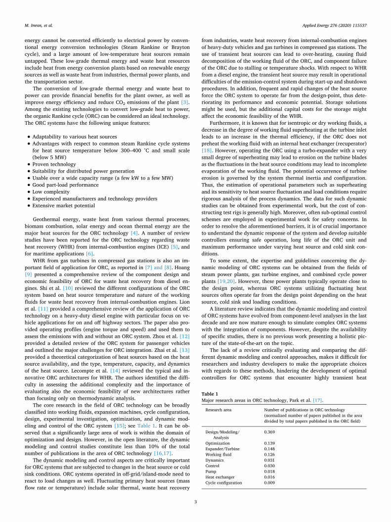
The core research in the field of ORC technology can be broadlyclassified into working fluids, expansion machines, cycle configuration,design, experimental investigation, optimization, and dynamic mod-eling and control of the ORC system [15]; see Table 1. It can be ob-served that a significantly large area of work is within the domain ofoptimization and design. However, in the open literature, the dynamicmodeling and control studies constitute less than 10% of the totalnumber of publications in the area of ORC technology [16,17].

The dynamic modeling and control aspects are critically importantfor ORC systems that are subjected to changes in the heat source or coldsink conditions. ORC systems operated in off-grid/island-mode need toreact to load changes as well. Fluctuating primary heat sources (massflow rate or temperature) include solar thermal, waste heat recovery

from industries, waste heat recovery from internal-combustion enginesof heavy-duty vehicles and gas turbines in compressed gas stations. Theuse of transient heat sources can lead to over-heating, causing fluiddecomposition of the working fluid of the ORC, and component failureof the ORC due to stalling or temperature shocks. With respect to WHRfrom a diesel engine, the transient heat source may result in operationaldifficulties of the emission-control system during start-up and shutdownprocedures. In addition, frequent and rapid changes of the heat sourceforce the ORC system to operate far from the design-point, thus dete-riorating its performance and economic potential. Storage solutionsmight be used, but the additional capital costs for the storage mightaffect the economic feasibility of the WHR.

Furthermore, it is known that for isentropic or dry working fluids, adecrease in the degree of working fluid superheating at the turbine inletleads to an increase in the thermal efficiency, if the ORC does notpreheat the working fluid with an internal heat exchanger (recuperator)[18]. However, operating the ORC using a turbo-expander with a verysmall degree of superheating may lead to erosion on the turbine bladesas the fluctuations in the heat source conditions may lead to incompleteevaporation of the working fluid. The potential occurrence of turbineerosion is governed by the system thermal inertia and configuration.Thus, the estimation of operational parameters such as superheatingand its sensitivity to heat source fluctuation and load conditions requirerigorous analysis of the process dynamics. The data for such dynamicstudies can be obtained from experimental work, but the cost of con-structing test rigs is generally high. Moreover, often sub-optimal controlschemes are employed in experimental work for safety concerns. Inorder to resolve the aforementioned barriers, it is of crucial importanceto understand the dynamic response of the system and develop suitablecontrollers ensuring safe operation, long life of the ORC unit andmaximum performance under varying heat source and cold sink con-ditions.

To some extent, the expertise and guidelines concerning the dy-namic modeling of ORC systems can be obtained from the fields ofsteam power plants, gas turbine engines, and combined cycle powerplants [19,20]. However, these power plants typically operate close tothe design point, whereas ORC systems utilizing fluctuating heatsources often operate far from the design point depending on the heatsource, cold sink and loading conditions.

A literature review indicates that the dynamic modeling and controlof ORC systems have evolved from component-level analyses in the lastdecade and are now mature enough to simulate complex ORC systemswith the integration of components. However, despite the availabilityof specific studies, there is no previous work presenting a holistic pic-ture of the state-of-the-art on the topic.

The lack of a review critically evaluating and comparing the dif-ferent dynamic modeling and control approaches, makes it difficult forresearchers and industry developers to make the appropriate choiceswith regards to these methods, hindering the development of optimalcontrollers for ORC systems that encounter highly transient heat

Table 1Major research areas in ORC technology, Park et al. [17].

Research area Number of publications in ORC technology(normalized number of papers published in the areadivided by total papers published in the ORC field)

Design/Modeling/Analysis

0.369

Optimization 0.139Expander/Turbine 0.148Working fluid 0.126Dynamics 0.031Control 0.030Pump 0.018Heat exchanger 0.016Cycle configuration 0.009


3

sources. Consequently, the lack of a holistic review may impede thecommercialization of ORC systems for applications characterized byhighly transient heat sources (e.g. the truck industry).

This paper provides a comprehensive review of the dynamic mod-eling and control of ORC systems. The component-level modeling isdiscussed, as well as the integration of components to form and modelcomplex systems; the technical difficulties, simulation pitfalls, bestpractices, and different modeling techniques are presented in detail.Various control schemes are compared, and the advantages, dis-advantages and maturity level for each of them are discussed. The moresuitable dynamic models of each component, solutions to commonproblems, and optimal control approaches are identified. Directions forfuture research are provided. Overall, the paper provides a unique,unified reference benchmark for future work concerning dynamicmodeling and control of ORC systems.

The paper consists of five sections. The introduction and state-of-the-art review are presented in Section 1. Section 2 discusses thecommon dynamic modeling approaches of ORC systems, both at thecomponent and the system-level. The control approaches for ORC

systems and their merits and demerits are discussed in Section 3. Dy-namic modeling and controller development tools and software arecovered in Section 4. Finally, the concluding remarks are presented inSection 5.

2. Dynamic modeling

This section provides a detailed description of the methodology andstate-of-the-art approach used for the dynamic modeling of the ORCcomponents, namely, the heat exchangers (evaporator and condenser),expander, pump, control valves, and storage tank. The modeling ofsingle-phase heat exchangers, such as preheaters, subcoolers and re-cuperators, can be derived from the evaporator and condenser models,considering that the working fluid is found only at the liquid or only atthe vapor phase under normal operation.

The control of the ORC system is based on its dynamic response.Therefore, understanding the process dynamics plays a critical role for asuccessful controller design. The dynamic response of the ORC systemdepends on a number of factors, such as cycle configuration, type of the

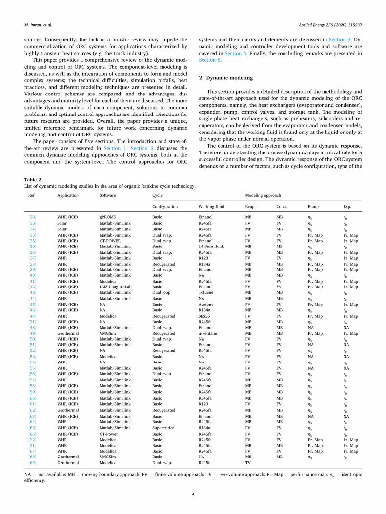
Table 2List of dynamic modeling studies in the area of organic Rankine cycle technology.

Ref. Application Software Cycle Modeling approach

Configuration Working fluid Evap. Cond. Pump Exp.

[28] WHR (ICE) gPROMS Basic Ethanol MB MB is is[33] Solar Matlab/Simulink Basic R245fa FV FV is is[34] Solar Matlab/Simulink Basic R245fa MB MB is is[35] WHR (ICE) Matlab/Simulink Dual evap. R245fa FV FV Pr. Map Pr. Map[35] WHR (ICE) GT-POWER Dual evap. Ethanol FV FV Pr. Map Pr. Map[29] WHR (ICE) Matlab/Simulink Basic 14 Pure fluids MB MB is is[36] WHR (ICE) Matlab/Simulink Dual evap. R245fa MB MB Pr. Map Pr. Map[37] WHR Matlab/Simulink Basic R123 FV FV is Pr. Map[38] WHR Matlab/Simulink Recuperated R134a MB MB Pr. Map Pr. Map[39] WHR (ICE) Matlab/Simulink Dual evap. Ethanol MB MB Pr. Map Pr. Map[40] WHR (ICE) Matlab/Simulink Basic NA MB MB is is[41] WHR (ICE) Modelica Basic R245fa FV FV Pr. Map Pr. Map[42] WHR (ICE) LMS Imagine.Lab Basic Ethanol FV FV Pr. Map Pr. Map[43] WHR (ICE) Matlab/Simulink Dual loop Toluene MB MB is is[44] WHR Matlab/Simulink Basic NA MB MB is is[45] WHR (ICE) NA Basic Acetone FV FV Pr. Map Pr. Map[46] WHR (ICE) NA Basic R134a MB MB is is[47] WHR Modelica Recuperated SES36 FV FV Pr. Map Pr. Map[31] WHR (ICE) NA Basic R245fa MB MB is is[48] WHR (ICE) Matlab/Simulink Dual evap. Ethanol MB MB NA NA[49] Geothermal VMGSim Recuperated n-Pentane MB MB Pr. Map Pr. Map[50] WHR (ICE) Matlab/Simulink Dual evap. NA FV FV is is[51] WHR (ICE) Matlab/Simulink Basic Ethanol FV FV NA NA[52] WHR (ICE) NA Recuperated R245fa FV FV is is[53] WHR (ICE) Modelica Basic NA FV FV NA NA[54] WHR NA Basic NA FV FV is is[55] WHR Matlab/Simulink Basic R245fa FV FV NA NA[56] WHR (ICE) Matlab/Simulink Dual evap. Ethanol FV FV is is[57] WHR Matlab/Simulink Basic R245fa MB MB is is[58] WHR (ICE) Matlab/Simulink Basic Ethanol MB MB is is[59] WHR (ICE) Matlab/Simulink Basic R245fa MB MB is is[60] WHR (ICE) Matlab/Simulink Basic R245fa MB MB is is[61] WHR (ICE) Matlab/Simulink Basic R123 FV FV is is[62] Geothermal Matlab/Simulink Recuperated R245fa MB MB is is[63] WHR (ICE) Matlab/Simulink Basic Ethanol MB MB NA NA[64] WHR Matlab/Simulink Basic R245fa MB MB is is[65] WHR (ICE) Matlab/Simulink Supercritical R134a FV FV is is[66] WHR (ICE) GT-Power Basic R245fa FV FV is is[22] WHR Modelica Basic R245fa FV FV Pr. Map Pr. Map[21] WHR Modelica Basic R245fa MB MB Pr. Map Pr. Map[67] WHR Modelica Basic R245fa FV FV Pr. Map Pr. Map[68] Geothermal VMGSim Basic NA MB MB is is[69] Geothermal Modelica Dual evap. R245fa TV – – –

NA = not available; MB = moving boundary approach; FV = finite volume approach; TV = two-volume approach; Pr. Map = performance map; is = isentropicefficiency.


4

components, and working fluid.The modeling paradigm to study the dynamics of the ORC tech-

nology used today is mostly modular, rather than simultaneous. Theprinciple of modularity implies that the outputs of a module (compo-nent model) must be dependent on the inputs of the module and be afunction of internal parameters only. This allows for the reusability of amodel and for using a bottom-up approach to develop libraries ofcomponents for easy application and reconfiguration. On the otherhand, the use of a simultaneous modeling approach fixes the system as awhole and generates a computationally efficient code; however, thistechnique does not allow modifications to be easily done to the model,and the set of equations needs to be rewritten if a component is added.

The interest in dynamic modeling goes back to 2007 when Colonnaet al. [19,20] presented a dynamic modeling paradigm for a steamRankine cycle and experimentally validated the results against mea-surements from a steam power plant. Wei et al. [21] presented twoalternative approaches for a dynamic model for the design of heat ex-changers of an ORC unit in 2007. Quoilin et al. [22] presented a dy-namic model and control strategy for a varying heat source in 2011. In2013, Casella at al. [23] presented a software library [24] includingmodular, reusable ORC components which were experimentally vali-dated against a commercial ORC unit. Later, Quoilin et al. [25] reportedthe development of a library for the dynamic simulation of thermo-dynamic systems in the object-oriented language Modelica. Pierobonet al. [26] presented a novel approach to integrate the dynamic per-formance of the ORC system into the preliminary design phase. Thenumerical model performed the thermodynamic cycle calculation andthe design of the components of the system. The results of these si-mulations were used within the framework of a multi-objective opti-mization procedure to identify a number of equally optimal systemconfigurations. A dynamic model of each of these systems was auto-matically parameterized, by inheriting its parameter values from thedesign model. Lakhani et al. [27] presented a dynamic modelingscheme of an ORC-based solar thermal power system with an integratedmulti-tube shell and tube thermal storage system in 2017. Recently,Hustler et al. [28] presented a validated dynamic model of an ORC unitfor waste heat recovery in a diesel truck. In addition, the thermo-phy-sical properties of the working fluids (such as heat capacity, latent heat,critical temperature, and density) affect the dynamic response of theORC system. Shu et al. [29] investigated the dynamic response of 14different working fluids based on the rise time, settling time and timeconstant. The results suggest that the working fluids with low criticaltemperature provide a faster response than those of working fluids witha high critical temperature.

Colonna et al. [19] recognized a difference between simultaneousand modular paradigms classifying the causal and non-causal models.In causal models, the systems are decomposed into computational

blocks with predefined causal interactions. This implies that inputvariables to the system must be decided prior to the development of theoverall model, and the resulting model will have certain rigidity tied tothe boundary and initial conditions, resulting in an explicit state-spaceform. However, bilateral coupling, discussed in detail in Ref. [19], canbe used to choose input and output variables. The early computer sol-vers were able to work with causal models only, and often there was aneed to manually reduce differential algebraic equations (DAEs) toordinary differential equations (ODE), increasing chances of errors andmodeling efforts. Modern solvers can handle non-causal models andsimplify the models using computer algebra and reorder the equationsdepending upon the choice of input and output variables, simplifyingthe work for the user.

The ORC component modeling generally involves the solution ofthree conservation equations for each component, namely, the energy,mass and linear momentum balances. In addition, there are oftenneeded constitutive equations, which can include heat transfer andpressure drop correlations and thermodynamic fluid property relations.

Depending on the accuracy and computational time, dynamicmodels can be classified into two categories: data-driven and physics-based models [22]. The data-driven models are based on the knowledgeof the system coming from measurements or previous simulations, andmake use of computational methods such as machine learning [30] ortransfer function identification to develop models of high computa-tional efficiency [31]. The drawback is that the accuracy of the model ishighly dependent on the quality of the data set [32]. Extrapolation outof the operating range of the data set can lead to poor accuracy andestimation errors. If there are modifications to the original system, themodel cannot be adapted if physical information is missing. Physics-based models are component-level models based on the conservationlaws (mass, energy and momentum). For this reason, changes in thesystem configuration and tests of the system performance in extremeoperating conditions can be assessed more easily. The complexity ofboth data-driven and physics-based models can change according to therequired accuracy and computational time. Low-order models are de-veloped by doing several simplifications in physics-based models aswell as by selecting a lower number of independent variables for data-driven models. They can be used for real-time applications and forlonger time simulations, such as annual simulations. High-order modelsare suited for shorter time period simulations, spanning from a fewminutes to several hours, when the computation time is not critical, andthese are the ideal choice for the development of controllers of broaderapplicability.

A list is shown in Table 2 of the dynamic modeling studies of ORCsystems and the applied modeling approaches.

Fig. 1. Time response of (a) gas turbine and (b) drum pressure of a gas-fired combined cycle power plant [71].


5

2.1. Heat exchangers

The dynamic response of the ORC system is mainly governed by theheat exchangers. The heat exchangers account for the majority of per-formance lag due to dynamic changes in the operating conditions. Thisis because the time constant of the heat exchangers is much larger thanthose of expanders and pumps, and mechanical transients are muchfaster than heat transfer phenomena. This is valid not only for ORCsystems [22,23], but also for conventional thermal power generationplants [70]. For instance, Shin et al. [71] studied the response time of agas-fired combined cycle power plant to rapid changes in the gas tur-bine load. As it can be seen in Fig. 1, the gas turbine could reach stableoperation in 4 s, whereas the steam generator required more than 200 sfor the high pressure part and 2000 s for the low pressure part to reachsteady operation.

In the particular case of heat exchangers involving two-phase flows,two commonly adopted heat exchanger modeling approaches are thefinite volume and the moving boundary methods. Both methods arebased on the conservation laws of energy, mass and momentum for adefined control volume. A third modeling approach, based on two vo-lumes in non-equilibrium, is also illustrated. The conservation equa-tions required to model the heat exchanger are mass, momentum andenergy balances for the heat source and working fluid.

2.1.1. Moving boundary methodIn a moving boundary (MB) model, the fluid flow in the heat ex-

changer is divided into as many control volumes as states of matter ofthe working fluid (i.e., liquid, two-phase, vapor) in the fluid flow. Thesize of the control volumes varies in real time during transient opera-tion, following the saturated liquid and the saturated vapor boundaries.A moving boundary model of an evaporator is shown in Fig. 2. Solving amoving boundary model is a non-linear implicit problem that leads toconvergence issues if proper guessed values are not provided [72].

The issues related to the guessed values decrease the robustness ofthe proposed models. The set of non-linear systems of equations of theMB is generally solved using the Newton solver [73]. However, thecomputational effort of the model depends on whether the system of theequations is presented in a causal formulation or an acausal formula-tion.

The mass balance of the working fluid is given by:

+ =A

tm

z( )

0wf XA wf wf,

(1)

Since there is no mass entering and leaving the wall, there is noneed for a mass balance of the wall. Generally, the dynamics of the heatsource are fast enough, leading the term m

zhs to be close to zero.

Therefore, it is not necessary to apply a mass balance for the heatsource. The energy balance of the working fluid and exhaust gas sharethe same general form, given by:

+ = =A h pA

tmh

zD U T T D U T

( )( )hs XA hs XA

eq w wf eq, ,

(2)

Deq is the effective flow path diameter for either the working fluidand exhaust gas, U is the overall heat transfer coefficient, and T is thetemperature difference between the fluid (working fluid or exhaust gas)and the wall. The energy balance of the wall is given by:

= +A c L dTdt

U A T U A Tw XA p w w ww

wf w wf w wf w hs w hs w hs w, , , , , , , , (3)

where subscript w represents the wall, cp is heat capacity, Lw is thelength in the axial direction, Aw,XA is the heat transfer area betweenworking fluid and the wall, Uwf,w is the heat transfer coefficient betweenworking fluid and the wall, Twf,w is the temperature difference be-tween the wall and the working fluid, is the heat exchanger efficiencymultiplier, which accounts for heat loss to the environment, Ahs w, is theheat transfer area between the exhaust gas and the wall, andUhs w, is the

heat transfer coefficient between the exhaust gas and the wall.The linear momentum balance is typically considered to be static,

and if the pressure drop is neglected, the balance becomes trivial:

=pz

0wf

(4)

Eqs. (1)–(4) represent the generalized forms of the mass, energy andlinear momentum balances of the heat exchangers. These equationsneed to be extended to the subcooled, two-phase, and superheated re-gions in the moving boundary model of the heat exchangers.

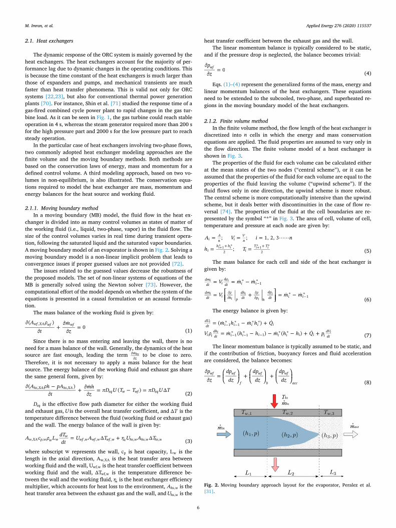
2.1.2. Finite volume methodIn the finite volume method, the flow length of the heat exchanger is

discretized into n cells in which the energy and mass conservationequations are applied. The fluid properties are assumed to vary only inthe flow direction. The finite volume model of a heat exchanger isshown in Fig. 3.

The properties of the fluid for each volume can be calculated eitherat the mean states of the two nodes (“central scheme”), or it can beassumed that the properties of the fluid for each volume are equal to theproperties of the fluid leaving the volume (“upwind scheme”). If thefluid flows only in one direction, the upwind scheme is more robust.The central scheme is more computationally intensive than the upwindscheme, but it deals better with discontinuities in the case of flow re-versal [74]. The properties of the fluid at the cell boundaries are re-presented by the symbol “*” in Fig. 3. The area of cell, volume of cell,temperature and pressure at each node are given by:

= = =

= =+ ++ +

A V i n

h T

; ; 1, 2, 3

;

iAn i

Vn

ih h

iT T

2 2i i i i1 1

(5)

The mass balance for each cell and side of the heat exchanger isgiven by:

= =

= + =

V m m

V m m

dmdt i

ddt i i

dmdt i h p

dhdt p h

dpdt i i

1

1

i i

ii

ii

i

(6)

The energy balance is given by:

= +

= + +

m h m h Q

V m h h m h h Q p

( )

( ) ( )

dUdt i i i i i

i idhdt i i i i i i i i

dVdt

1 1

1 1 1

i

i i(7)

The linear momentum balance is typically assumed to be static, andif the contribution of friction, buoyancy forces and fluid accelerationare considered, the balance becomes:

= + +pz

dpdz

dpdz

dpdz

wf wf

f

wf

b

wf

acc (8)

Fig. 2. Moving boundary approach layout for the evaporator, Peralez et al.[31].


6

2.1.3. Comparison of moving boundary and finite volume methodFor a dynamic simulation of the ORC system, Wei et al. [21] com-

pared the moving boundary and discretization technique approach.Their results suggested that both approaches can predict the dynamicperformance of the ORC system fairly well, with less than 4% relativedifference compared with the experimental results. The simulation doesnot show the numerical chattering or oscillations in the results. As forthe FV model, the level of discretization plays a critical role in the ac-curacy, computational effort and numerical inconsistencies.

As a general rule of thumb, a minimum number of 20 nodes is re-commended to avoid numerical inconsistency in the simulation results[76]. The level of discretization might affect the working fluid phaseboundary from one cell to the next, which would generate a numericalmass flow rate due to the discontinuity characterizing the density in theregions around the saturation lines [77]. Desideri et al. [76] developed

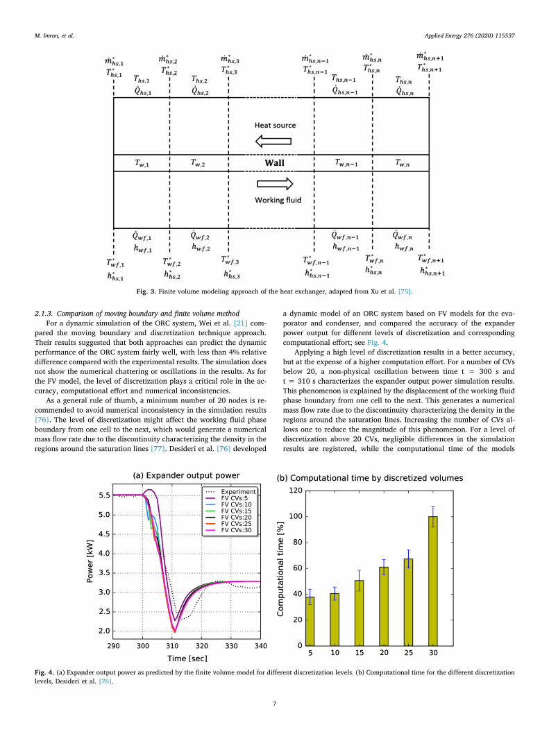
a dynamic model of an ORC system based on FV models for the eva-porator and condenser, and compared the accuracy of the expanderpower output for different levels of discretization and correspondingcomputational effort; see Fig. 4.

Applying a high level of discretization results in a better accuracy,but at the expense of a higher computation effort. For a number of CVsbelow 20, a non-physical oscillation between time t = 300 s andt = 310 s characterizes the expander output power simulation results.This phenomenon is explained by the displacement of the working fluidphase boundary from one cell to the next. This generates a numericalmass flow rate due to the discontinuity characterizing the density in theregions around the saturation lines. Increasing the number of CVs al-lows one to reduce the magnitude of this phenomenon. For a level ofdiscretization above 20 CVs, negligible differences in the simulationresults are registered, while the computational time of the models

Fig. 3. Finite volume modeling approach of the heat exchanger, adapted from Xu et al. [75].

Fig. 4. (a) Expander output power as predicted by the finite volume model for different discretization levels. (b) Computational time for the different discretizationlevels, Desideri et al. [76].


7

increases significantly, as shown in Fig. 4b. This analysis allows one toidentify a level of discretization of 20 CVs as a good compromise be-tween accuracy and simulation speed for this specific simulation.

Although the heat transfer and pressure drop correlations provideaccurate assessments of the heat transfer and pressure drop, it is gen-erally difficult to use these correlations for dynamic simulations as theymay slow down the calculation process, and potentially cause numer-ical instabilities and simulation failure. Quoilin et al. [78] proposed afast, robust approach to model heat transfer. At nominal conditions, theheat transfer coefficient is determined and termed as the nominal heattransfer coefficient. For situations other than nominal conditions, theheat transfer coefficient is computed as follows:

= mmn

n

m

(9)

and n are the heat transfer coefficient at the given state and thenominal heat transfer coefficient, m mand n are the mass flow rate ofworking fluid at the given state and the nominal mass flow rate, andmisa constant that depends on the heat transfer correlation.

The heat transfer coefficient can also be calculated using Eq. (10)[78]. The transitions between the different heat transfer coefficients(liquid, two phase, and vapour) may cause inconsistency and simula-tion failure. The non-zero quality, x,width based transition by inter-polating between the heat transfer coefficients can resolve this issue. Inthe interpolation function, the heat coefficients are represented in theform of vapor quality, x . The vapor quality is defined by an enthalpy

ratio as presented in Eq. (10). This results in a smooth function as thevapor quality and its first derivative are continuous. This continuityavoids negative effects in the solution process.

=

<

+ <

<

+ < +

+

=

+

+

( )

( )

if x x

if x x

if x x

if x x

if x x

x

/2

· /2

1 /2

· 1 /2

1 /2

liq

liqsin x x

tp

tpsin x x

vp

h hh h

( )2

1 ( / )2

( )2

1 ( ( 1) / )2

tp liq

vp tp

ll v (10)

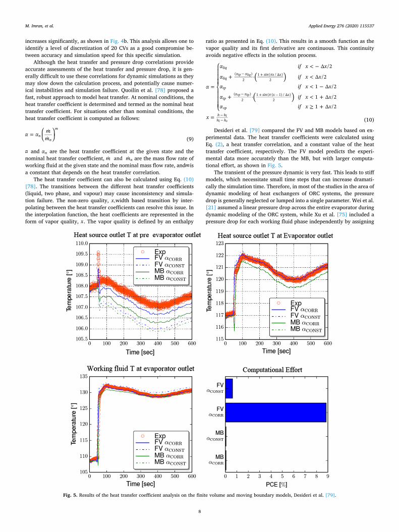
Desideri et al. [79] compared the FV and MB models based on ex-perimental data. The heat transfer coefficients were calculated usingEq. (2), a heat transfer correlation, and a constant value of the heattransfer coefficient, respectively. The FV model predicts the experi-mental data more accurately than the MB, but with larger computa-tional effort, as shown in Fig. 5.

The transient of the pressure dynamic is very fast. This leads to stiffmodels, which necessitate small time steps that can increase dramati-cally the simulation time. Therefore, in most of the studies in the area ofdynamic modeling of heat exchangers of ORC systems, the pressuredrop is generally neglected or lumped into a single parameter. Wei et al.[21] assumed a linear pressure drop across the entire evaporator duringdynamic modeling of the ORC system, while Xu et al. [75] included apressure drop for each working fluid phase independently by assigning

Fig. 5. Results of the heat transfer coefficient analysis on the finite volume and moving boundary models, Desideri et al. [79].


8

each phase its own linear pressure drop along the spatial length in thedynamic modeling of an ORC system.

The heat exchanger dynamic modeling is typically limited to one-dimensional modeling approaches, since two and three-dimensionalspatial models bring a level of computational and analytical complexitythat is unsuitable for the purposes of multi-component dynamic mod-eling and control.

The moving boundary modeling approach is much faster (by ap-proximately three times) than the finite volume approach. However,the moving boundary approach has a lower accuracy than the finitevolume approach when compared with experimental data. In addition,the moving boundary approach is more difficult to implement due tothe complexity of variable control volume lengths, the need to in-corporate the mean void fraction and the difficulty to extend the modelto various heat exchanger types and geometries. The finite volumeapproach is simple, easy to derive, and easy to implement with variousheat exchanger types and geometries due to the ease in reconfigurationof the model.

Furthermore, the finite volume method can provide additional va-lues of the heat exchanger parameters, while the moving boundarymethod only provides values for the outlet of the component andlumped values. For example, the finite volume approach can providethe tube wall temperature at uniform length intervals along the lengthof the tube, while the moving boundary model only provides thelumped value for each working fluid phase.

Refer to Table 2 for the list of modelling methods applied to ORCsystems.

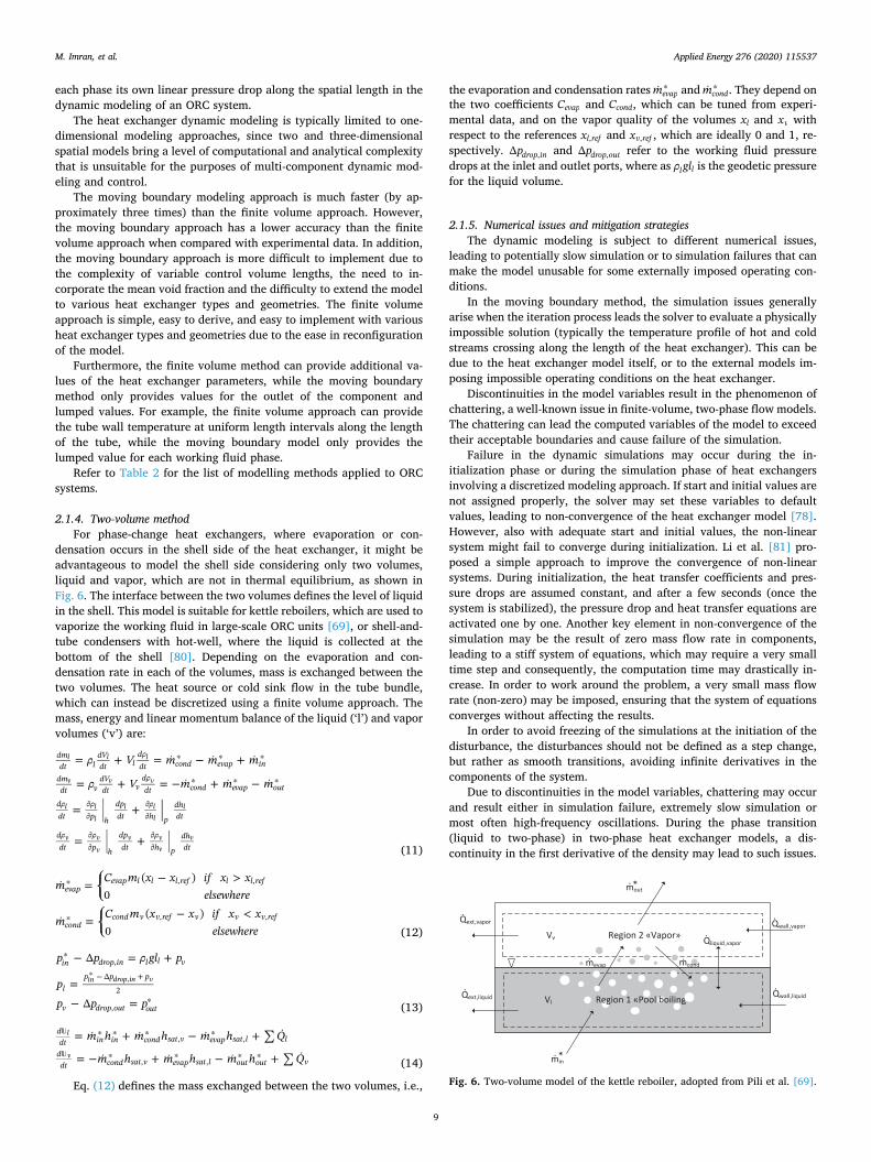
2.1.4. Two-volume methodFor phase-change heat exchangers, where evaporation or con-

densation occurs in the shell side of the heat exchanger, it might beadvantageous to model the shell side considering only two volumes,liquid and vapor, which are not in thermal equilibrium, as shown inFig. 6. The interface between the two volumes defines the level of liquidin the shell. This model is suitable for kettle reboilers, which are used tovaporize the working fluid in large-scale ORC units [69], or shell-and-tube condensers with hot-well, where the liquid is collected at thebottom of the shell [80]. Depending on the evaporation and con-densation rate in each of the volumes, mass is exchanged between thetwo volumes. The heat source or cold sink flow in the tube bundle,which can instead be discretized using a finite volume approach. Themass, energy and linear momentum balance of the liquid (‘l’) and vaporvolumes (‘v’) are:

= + = +

= + = +

= +

= +

V m m m

V m m m

dmdt l

dVdt l

ddt cond evap in

dmdt v

dVdt v

ddt cond evap out

ddt p h

dpdt h p

dhdt

ddt p h

dpdt h p

dhdt

l l l

v v v

l ll

l ll

l

v vv

v vv

v

(11)

= >

= <

m C m x x if x xelsewhere

m C m x x if x xelsewhere

( )0

( )0

evapevap l l l ref l l ref

condcond v v ref v v v ref

, ,

, ,

(12)

= +

==

+

p p gl p

pp p p

in drop in l l v

lp p p

v drop out out

,

2

,

in drop in v,

(13)

= + +

= + +

m h m h m h Q

m h m h m h Q

ddt in in cond sat v evap sat l l

ddt cond sat v evap sat l out out v

, ,

, ,

l

v(14)

Eq. (12) defines the mass exchanged between the two volumes, i.e.,

the evaporation and condensation ratesmevap andmcond. They depend onthe two coefficients Cevap and Ccond, which can be tuned from experi-mental data, and on the vapor quality of the volumes xl and xv withrespect to the references xl ref, and xv ref, , which are ideally 0 and 1, re-spectively. pdrop in, and pdrop out, refer to the working fluid pressuredrops at the inlet and outlet ports, where as gll l is the geodetic pressurefor the liquid volume.

2.1.5. Numerical issues and mitigation strategiesThe dynamic modeling is subject to different numerical issues,

leading to potentially slow simulation or to simulation failures that canmake the model unusable for some externally imposed operating con-ditions.

In the moving boundary method, the simulation issues generallyarise when the iteration process leads the solver to evaluate a physicallyimpossible solution (typically the temperature profile of hot and coldstreams crossing along the length of the heat exchanger). This can bedue to the heat exchanger model itself, or to the external models im-posing impossible operating conditions on the heat exchanger.

Discontinuities in the model variables result in the phenomenon ofchattering, a well-known issue in finite-volume, two-phase flow models.The chattering can lead the computed variables of the model to exceedtheir acceptable boundaries and cause failure of the simulation.

Failure in the dynamic simulations may occur during the in-itialization phase or during the simulation phase of heat exchangersinvolving a discretized modeling approach. If start and initial values arenot assigned properly, the solver may set these variables to defaultvalues, leading to non-convergence of the heat exchanger model [78].However, also with adequate start and initial values, the non-linearsystem might fail to converge during initialization. Li et al. [81] pro-posed a simple approach to improve the convergence of non-linearsystems. During initialization, the heat transfer coefficients and pres-sure drops are assumed constant, and after a few seconds (once thesystem is stabilized), the pressure drop and heat transfer equations areactivated one by one. Another key element in non-convergence of thesimulation may be the result of zero mass flow rate in components,leading to a stiff system of equations, which may require a very smalltime step and consequently, the computation time may drastically in-crease. In order to work around the problem, a very small mass flowrate (non-zero) may be imposed, ensuring that the system of equationsconverges without affecting the results.

In order to avoid freezing of the simulations at the initiation of thedisturbance, the disturbances should not be defined as a step change,but rather as smooth transitions, avoiding infinite derivatives in thecomponents of the system.

Due to discontinuities in the model variables, chattering may occurand result either in simulation failure, extremely slow simulation ormost often high-frequency oscillations. During the phase transition(liquid to two-phase) in two-phase heat exchanger models, a dis-continuity in the first derivative of the density may lead to such issues.

Region 1 «Pool boiling»

Region 2 «Vapor»

mout

mevap

min

mcond

Vl

Vv

Qwall,vapor

Qwall,liquid

Qliquid,vapor

Qext,vapor

Qext,liquid

.

.

.

.

..

.

.

. *

*

Fig. 6. Two-volume model of the kettle reboiler, adopted from Pili et al. [69].


9

The simulation may fail or result in a stiff system if the cell-generated(and purely numerical) flow rate due to this discontinuity causes a flowreversal in one of the nodes as well as oscillations in pressure. Quoilinet al. [77] carried out a comprehensive analysis of the issues linked tosimulation failures during integration in finite-volume flow models andprovided several methods to tackle chattering and flow reversal pro-blems. A filtering method, truncation method, smoothing of the densityfunction and density derivative, a mean densities method, an enthalpylimiter method, and a smooth reversal enthalpy method were suggestedto tackle such simulation failures and resolve these issues [77].

2.2. Expander

For the dynamic modeling of ORC systems, the time constantscharacterizing the expansion and compression processes are smallcompared to those of the heat exchangers. Thus, the models for theexpansion machine can be based on empirical or semi-empirical alge-braic correlations where dynamics are neglected, i.e., a lumped modelbased on performance curves or the semi-empirical model developed byLemort et al. [82].

There are two types of expansion machines for ORC systems, thevolumetric expander and the turbo-expander. The choice of the type ofexpander is dependent on the system design, size, and application.Since the residence time of the working fluid in the expander is rela-tively small in comparison to those of the evaporator and condenser,the use of a static model is preferred for the modeling of the expansionmachine. The model of the expander should include both the first andsecond thermodynamic laws. The first law includes the dependenciesamong pressure, flow rate, and rotational speed, while the second lawrelates the isentropic efficiency with the flow rate and pressure as wellas the rotational speed [83].

2.2.1. Volumetric expanderThe dynamics of the expander and the pump are very fast compared

to those of the evaporator and condenser and are modeled at steady-state. Neglecting the heat loss, a volumetric expander can be modeledby its isentropic efficiency and filling factor, given by:

=W

m h h( )exp isexp

wf exp in exp out,

, , (15)

=m

V Nwf

exp in sw exp, (16)

The outlet enthalpy is given by:

=h h h h( )exp out exp in exp is exp in exp out is, , , , , , (17)

In the case that experimental data are available, a performance mapof a volumetric expander can be obtained, predicting the isentropicefficiency as a function of the expander inlet pressure, expander rota-tional speed, and expander pressure ratio (see e.g. Ref. [47]). The massflow rate through an expander is given by:

=m V Nwf exp in sw exp, (18)

The losses of volumetric expanders include leakage losses, under-and over-expansion losses, friction losses, and heat losses. In order toobtain an accurate result, the work done by a volumetric expandershould be calculated considering both the under-expansion and over-expansion losses [22,57]. Quoilin et al. [84] presented a detailed semi-empirical model of a scroll expander, accounting for heat losses,working fluid leakage loss, and under-expansion and over-expansionlosses. The model is based on the physics of the expansion processacross the machine, where a few unknown parameters are tuned byfitting with experimental data.

2.2.2. Turbo-expanderThe dynamic of the turbine is very fast compared to that of the heat

exchangers, and thus the turbine model is at steady-state. A perfor-mance map of the turbine can be used to calculate the mass flow ratethrough the turbine as a function of the rotational speed and pressureratio:

=m performance map N p( , )wf exp in exp, (19)

Xu et al. [75] used the turbine inlet temperature and Wei et al. [21]used the pressure ratio from the turbine performance map to calculatethe mass flow rate through the turbine. The semi-empirical formulationof the Stodola equation [85] can be used to calculate the mass flow rateof the working fluid through the turbine:

=

=

m K p PR

PR

(1 ( ) )wf exp eq in exp in exppp

, , ,2

in exp

out exp

,

, (20)

The Keq integrates the equivalent inlet nozzle cross-section and thedischarge coefficient and is calculated from the turbine performance atthe nominal condition:

=Km

p PR( )

( ) ( ) [1 ( ) ]eq

wf exp n

in exp n in exp n n

,

, ,2

(21)

The enthalpy at the outlet of the turbine is given by:

=h h h h( )out exp in exp exp is in exp out is exp, , , , , , (22)

In most of the previous studies, the isentropic efficiency of theturbine was assumed constant. However, since the ORC system mostlyoperates far from design point in transient conditions, assuming aconstant isentropic efficiency may lead to significant errors in the dy-namic response of the ORC system [83]. Also the part-load performancein steady-state conditions will be inaccurately predicted by assuming aconstant isentropic efficiency of the expander. An alternative to as-suming a constant is to obtain the turbine isentropic efficiency from aturbine performance map, as in e.g. Xu et al. [75]:

= performance map N PR T( , , )exp is exp exp in exp, , (23)

The power output of the expander is given by:

=W m h h( )exp wf in exp out exp, , (24)

2.3. Pump

The dynamic response of the working fluid pump is very fast com-pared to that of the heat exchangers; hence, the pump is typicallymodeled using a steady-state lumped parameter model [60]. Suchmodel can be based on performance maps provided by the pumpmanufacturer. The performance chart includes head versus volume flowcurves at different rotational speeds. If the map is provided with onerotational speed only, curves at other speeds can be approximated bymeans of a kinematic similarity principle. Another type of performancechart includes efficiency curves on the head-flow plane or in terms ofpower consumption curves as a function of flow and speed [83]. Heatlosses to the environment are usually neglected.

For centrifugal pumps, the volume flow rate is a function of both thehead and the rotational speed. The crossing point between the char-acteristic curve of the system and the performance curve of the pumpdefines the operating point, as shown in Fig. 7.

For a positive-displacement pump, the mass flow rate through theworking fluid pump is obtained from the performance curve (pumpspeed vs mass flow rate). If the dependency on the pressure ratio isneglected:


10

== +

m performance map Nm C C f

( )wf pu pu

wf pu pu

,

, 1 (25)

where Npu is the pump speed, C and C1 are empirical constants, and fpuis the frequency of the pump motor. In case the performance maps arenot available, the mass flow rate can be obtained from the volumetricefficiency of the pump:

=m mwf wf ideal vol pu, , (26)

The volumetric efficiency, ,vol pu, is a function of the pump speedpump (revolutions per second) and the pressure ratio across the pump

[56]. The ideal mass flow rate of the pump is given by:

=m V Nwf ideal pd pu, (27)

Vpd is the pump displacement volume, and is the working fluiddensity. The pump power consumption and the outlet temperature aregiven by:

=Wm p p( )

puwf out pu in pu

is pu

, ,

, (28)

= +T Tm C

W(1 )

out pu in puis pu

wf pu p pupu, ,

,

, , (29)

The isentropic efficiency can also be expressed as a function ofknown parameters (polynomial fit) from the performance map of thepump provided by the manufacturer. These parameters may include thepump capacity fraction, Xpu cf, , defined by a reference [86].

=Xv m

Vpu cfin pu wf pu

in pu max,

, ,

, , (30)

Depending on the size of the pump, the pump capacity factor islimited by the boundary condition, V X 1su pu min pu cf, , , . The knownparameters in the polynomial fit can be represented by the mass flowrate fraction, Xpu mf, , given by [75]:

=Xm

mpu mfwf pu

wf pu max,

,

, , (31)

mwf pu, is mass flow rate at any given condition while mwf pu max, , ismaximum mass flow rate that pump can deliver. Desideri et al. [79]used a second-order polynomial, as a function of the non-dimensionalpressure ratio and non-dimensional pump frequency, to estimate theisentropic efficiency of the pump:

= + + + + +C C f C f C r C r C f r( ) ( )pu is pu pu pu pu pu pu, 1 12

3 42

5 (32)

In most of the simulation studies, the isentropic efficiency of thepump is assumed to be between 60% and 85%. However, a review of

the experimental data obtained for ORC systems indicates that theisentropic efficiency of the pump can be as low as 40% [16]. As with theexpander, assuming a constant isentropic efficiency may lead to in-accurate dynamic response or part-load predictions; however, in thisregard the influence of the pump is less than that of the expander. Thisis because the pump power is usually lower than 10% of the mechanicalpower at the turbine shaft.

Refer to Table 2 for the list of studies presenting performance esti-mation for pump and expander models.

2.4. Storage tank/liquid receiver

During the transient operation of the ORC system, the reservoir/storage tank acts as a buffer for the working fluid. The amount ofworking fluid charge and leakage can significantly alter the ORC systemdynamics. A system with over filled working fluid will lead to condi-tions, where the working fluid start accumulating in the condenser asliquid. This will result in a larger degree of sub-cooling and a highercondenser pressure resulting in reduced power output and decreasedefficiency.

The storage tank avoids the accumulation of working fluid in thecondenser. On the other hand, if the working fluid amount is too smallor working fluid has leaked out of the system, the system start-up willbecome almost impossible because during the start-up phase the pumpwill run out of working fluid and a cyclic flow may not be established.For the modelling of the storage tank (liquid receiver), it is usuallyassumed that the liquid and vapor phases are in thermodynamic equi-librium at all times, i.e., the vapor and liquid are assumed saturated atthe given pressure. The pressure drop is typically neglected. The massbalance is given by:

= = +dm

dtm m

dmdt

Vh

dhdt p

dpdt

; . · ·wfin wf out wf

wf

p h, ,

(33)

V is the volume of the liquid receiver tank in m3. The density of theliquid can be represented in terms of a liquid level fraction L (0 whenthe tank has only vapor, 1 when the tank is full of liquid), given by:

= +Y Y(1 )l v (34)

The term, Y , is the level of saturated liquid in the receiver tank ofthe ORC system. Inserting the equation for the density, Eq. (34), intothe mass balance equation, Eq. (33), gives the following equation:

+ + =V dYdt

ddt

Yddt

Y m m( )· · ·(1 )l vl v

in wf out wf, ,(35)

The generalized relation for the energy balance for the receiver tank[79] is given by:

= +h Y h Y h(1 )l l v v (36)

Substituting Eq. (36) into Eq. (7), the mass balance in receiver tankcan be represented as [79]:

+ + +

+ =

V dYdt

h h dpdt

Y hddp

dhdp

Y

hddp

dhdp

m h m h

( ) · (1 )·

1

l l v v ll

ll

vv

vv

in wf in out wf out, ,(37)

Another aspect of ORC system design is to avoid that the change inthe level/height of the receiver tank, at any time during operation,leads to a reduction of the net positive suction head available, becominglower than net positive suction head required by the pump. Based onthe level of working fluid in the receiver tank, the loss/leakage ofworking fluid charge quantity can be identified and working fluidquantity can be replenished.

Growing rotational speedHead

Volume flow rate

1

2Operating points

Pump characteristics

Pumping system characteristics

Fig. 7. Flow-head characteristics of a centrifugal pump.


11

2.5. Control valves

The dynamic characteristics of the control valve can be modeledwith relevant equations that correlate the valve opening, boundaryconditions and the flow through the component. The control valvemodel for WHR-based ORC systems is based on either the in-compressible flow for liquid flow or the compressible flow for vaporand two-phase flow [56]. If the system dynamics are fast, the valvepositioning servo-system plays an important role in determining theclosed-loop dynamic behavior of the system and should be included inthe model [83]. However, it is difficult to gain access to informationabout the servo-positioner dynamics; hence, first-order or second-orderlinear systems can be used to consider these dynamics.

In case experimental data are available for the ORC system, anempirical correlation can be developed to calculate the mass flow ratefor incompressible flow based on the relative valve openings. Xu et al.[75] used an empirical approach to estimate the incompressible flowrate through the control valve for a parallel evaporator ORC system. Inthe parallel evaporator configuration, the waste heat from an internalcombustion engine is recovered using two evaporators in a parallelarrangement, one recovers heat from the exhaust gas recirculation flowand the other from the exhaust gas tail pipe [75]. The mass flow rate forsuch configuration is given by:

= +m m mwf wf ev wf ev, 1 , 2 (38)

=rmmm

wf ev

wf ev

, 1

, 2 (39)

=r Cµµm d

vl

vl

c,1

,2

1

(40)

=+

m m rr 1wf ev wf

m

m, 1

(41)

=+

m mr

11wf ev wf

m, 2

(42)

The parameters µvl,1 and µvl,2 are the opening of valves 1 and 2,respectively, before each evaporator. The discharge coefficient, Cd, andthe constant c1 can be found by model identification [87]. The term, rm,is the mass flow rate ratio of the working fluid between the two eva-porators. For cases where experimental data are not available, the massflow rate through the valve for incompressible flow can be determinedas follows [56]:

=m µ C A p p2 ( )cv cv d O in out (43)

The thermodynamic state of the working fluid at the outlet is cal-culated assuming an isenthalpic process through the valve. The massflow rate through the valve for compressible flow is given by [75]:

+If

pp

subsonic21

1 ( )out

in

1

(44)

=+

m µ C A ppp

pp

21cv cv d O in in

out

in

out

in

2 1

(45)

+If

pp

supersonic0 21

( )out

in

1

(46)

=+

+

m µ C A p21cv cv d O in in

12( 1)

(47)

is the heat capacity ratio. Assuming an isentropic process acrossthe valve, the outlet temperature can be estimated by the enthalpy andpressure at the outlet of the valve. There is only one previous study [46]

that considered the internal structure of the servo valves to estimate thevalve opening.

2.6. Sensors

The measuring instruments might have a significant delayed re-sponse, especially the temperature sensors [83]. If the time scale of themeasuring instrument is not negligible compared to the closed loopresponse time, it should be included in the model. First or second-order,low-pass linear systems can be used for this purpose. Lemort et al.[53,88] modeled the delayed response of the pump actuator, tem-perature and pressure sensors by a first-order model with the help of themanufacturer data.

The dynamic modeling approach of the components of the ORCsystem are similar to conventional power plants such as combined cyclepower plant [89–92], coal fired power plant [93–95], nuclear powerplant [96–99], and concentrated solar power [100–102]. The dynamicmodeling of these systems was carried in Dymola and Simulink. Acomprehensive review of dynamic simulation, its development andapplication to various thermal power plants is presented in Ref. [70].The underlying flow models and their fundamental assumptions andcomponent level modeling of conventional thermal power plants arediscussed in detailed.

3. Controller design

The choice of working fluid, thermodynamic design, and mechan-ical design of the ORC components are prerequisite for the controllerdevelopment and are used as input data for the controller design.Initially, the specific and concrete goals of the control system should bedefined in terms of control variables and suitable set points. The maintasks of the control system are to keep the system safe and stable, tominimize the impact of disturbances and to optimize the ORC opera-tion. In order to avoid singularities in the trajectories of the system, thenumber of manipulated variables should be equal or higher than thenumber of control variables. In the most common case, they are chosenin equal number. In the next phase, the dynamic interactions among themanipulated variables and control variables are investigated by ana-lyzing the dynamic response of the control variables to step changes ormore generally rapid changes of the manipulated variables. The stepresponses and transfer functions can provide an insight to identifyingthe dominant time constants of the system, the fastest system variables,and the slowest system variables. The transfer functions can be devel-oped from experimental data or simulations of a physics-based model.Transfer functions are algebraic equations based on an input–outputrelationship, whereas the physics-based models are ordinary differ-ential equations described by means of inputs, outputs and states.

The basic control strategy of the ORC system can be divided intotwo basic approaches: following the connected load (FCL) and fol-lowing the thermal energy input (FTE) [103]. The number of actuatorswhich can be manipulated in the system, as well as the variables thatneed to be controlled and kept close to the set points, define the basiccontrol strategy. For instance, the rotational speed of the expander canbe kept constant or it can be varied according to the operating point foroptimal part-load performance.

In the FCL mode, the expander and the generator are linked with thesame shaft. A gearbox could be included to keep the same speed ratiobetween the expander and the generator, in the case they do not rotateat the same speed. In most cases, systems in FCL mode have the gen-erator connected to the power grid without a power converter interface.The grid frequency and the number of poles of the stator winding of thegenerator determine the rotational speed of the generator (and theexpander). The produced electric power from the generator needs tofollow the variations of the electric demand, while the ORC processvariables must be kept within safe operating limits. For this purpose,the heat source is controlled and adapted to the grid load. The FCL


12

mode without a frequency converter is depicted in Fig. 8.If a frequency converter is included, the rotational speed of the

expander can be used to control the upstream pressure of the expander,thus providing an additional degree of freedom. However, the operatingconditions of the ORC system may change substantially due to changesin the load requirements or expander speed.

In the FTE mode, the goal of the system is to maximize the elec-tricity production based on the heat available. The electric power fromthe generator follows the variations of heat source conditions. In anideal case, all the heat available is fed to the ORC and converted intoelectricity. Some control elements on the heat source stream might stillbe required for extreme conditions to avoid overloading and/or thermaldegradation of the working fluid. The FTE mode is shown in Fig. 9.Here, a frequency converter is included, but if not present, the rota-tional speed of the expander is kept constant.

In terms of a control strategy, the ORC system can be operated in thesliding pressure mode or the fixed pressure/variable mass flow mode, ora combination of both. However, these operational modes do not takeinto account the dynamic response of the ORC system. Nonetheless,they are useful for the part-load modeling of the ORC system and fordefining the controller set points.

The sliding pressure control involves changes in the evaporatorpressure resulting from the pump, evaporator and expander char-acteristics. The fixed pressured/variable mass flow rate scheme can beimplemented by the addition of a pressure control valve (throttlingvalve) at the expander inlet to maintain pressure at a constant level inthe evaporator, while the pump controls the mass flow rate through thecycle. This technique is easy to implement and might maintain a high-cycle efficiency (arguably theoretically) by keeping a high pressure atpart-load; however, the throttling of the valve results in exergy losses,and the evaporation process is not optimized for the different heatsource conditions (mismatches of the heat source and working fluidtemperature lines in the T-Q diagram), resulting in pinch-point limita-tions and sub-optimal operation. The fixed pressure operation might bechosen at low load to ensure practical operation of the system, avoidingexceeding the minimal load of the components. For these reasons, atmedium/nominal load range the sliding pressure mode is typicallypreferred. The operational strategy, which will then be important forthe controller set points, can be optimized offline without accountingfor the dynamics. If the dynamics is included, the controller requires aninternal optimization function (or a supervisory block) that defines its

actions by solving an online optimization problem.As for the control of ORC systems, previous works were often car-

ried out by validating a dynamic model against an open-loop responsecaused by a step disturbance or a set point change. The validatedmodels are then simulated/tested with a control algorithm im-plemented in a closed loop. However, in practice the ORC systemcontrol schemes are highly dependent on the application, type ofequipment and cycle configuration. The control scheme of a grid-con-nected unit is significantly different from that of a system in off-gridmode, because it can be assumed that larger plants in the grid willmainly be responsible for the stability of the grid in the first case,whereas in an off-grid system, the ORC unit has to ensure proper con-tribution to the frequency and voltage stability of the decentralizednetwork. Renewable-based off-grid ORC systems have been proposedmainly for remote areas [104].

Various works utilizing validated dynamic models and discussingcontrol schemes have been reported in the literature. Given the largeamount of control ideas that have been proposed, a brief overview ofthe main classes of controllers is provided here. The main techniquesare summarized in Fig. 10.

State-of-the-art ORC systems make use of proportional-integral-de-rivative (PID) controllers. These systems rely on the idea of directlyacting on the error between the set point and the control variable(output feedback control) [105]. They have the advantage of beingsimple and easily available as electronic modules. The tuning of thecontroller parameters can be carried out empirically, directly on theplant without the need of a model. Some simple guidelines for con-troller tuning have been developed, such as the Ziegler-Nichols rules[106].

Another approach makes use of an input–output description of alinear or linearized dynamic model of the unit, and then applies tech-niques developed from the analysis of the linear dynamic system. Formulti-variable systems, where more than a single pair input/output isconsidered, multiple PIDs that work independently of one another aretypically installed. Given the interdependency of the system variables,for instance, between the evaporator pressure and the degree of su-perheating at the evaporator outlet, a conflict between the two con-trollers or performance degradation can occur. Some methods exist todecouple the controller action and avoid the interdependency amongthe variables, but the stringent mathematical conditions on the systemproperties that must be maintained limit the applicability of these

Fig. 8. A schematic of the ORC system operating with the FCL mode, Zhang et al. [57].


13

methods. More measurements (not necessarily control variables) can befed to the same controller, to increase the amount of information that itreceives and improve its performance. This is the principle of cascadedcontrol. Additionally, since linear systems do not account for internaltime delays in the system, lead/lag compensators can be implementedto compensate for these phenomena. To conclude, another importantimprovement to classical PID controllers consists of including a feed-forward part acting on the manipulated variables. The feed-forwarddetects the disturbance or set point change and sets the manipulatedvariables to compensate directly for their impact before there is anynoticeable change in the system output, which is different from whatoccurs in the case of classical PID controllers based on output feedbackcontrol.

In addition to the classical control techniques based on PID con-trollers, the improvements made in computational science have en-hanced the development of advanced control methods, where thecontroller makes use of the computational power of modern processorsto design the controllers. Advanced controllers include optimal con-trollers (OC), adaptive controllers (AC) and model predictive con-trollers (MPC). Optimal controllers are designed to minimize a costfunction (optimization target). Optimal control methods include dy-namic programming (DP) and linear quadratic controllers (LQ). Bothmethods are based on a state-space model of the system, which givesinformation on the dynamics and time development of the system.

Dynamic programming is a technique that defines future decisionsbased on the previous ones, operating in a recursive manner. Thetechnique can be applied to both linear and non-linear systems, but indiscrete form. DP has the advantage of allowing for real-time optimi-zation of the controller set points. The main drawback is the compu-tational effort required to solve the optimal problem, especially if thesystem has more than one state or control input [107].

LQ controllers are based on a state-space linear or linearized dy-namic model of the system. They are a state-feedback technique andtherefore require the knowledge of the system state. If not all the statesare measurable, a state estimator (observer) has to be included toprovide information on the system states. The design of LQ controllersis based on a trade-off between the performance of the controller toreach the desired state and the energy required to control the actuators.In fact, it can be worth accepting a penalty on controller performance, ifthis results in a reduction of its energy consumption or in an increasedlifetime of the actuators. To reach this goal, a quadratic cost function isminimized to design the controller feedback matrix. LQ controllers canhandle multi-variable systems with no particular increase in com-plexity. The drawback when applied to non-linear systems is that thetechnique was developed for linear systems and cannot account for thenonlinear couplings between the systems variables. LQ controllerscannot be used if the system states cannot be measured or estimated.

Such state estimators (observers) have been developed both for

Fig. 9. A schematic of the ORC system operating with the FTE mode, Zhang et al. [57].

Control

Classical control

PID (output

feedback)

Cascaded control Feedforward Lead/lag

compensation

Advanced control

Optimal control

Dynamic programming

Linear quadratic Control

Adaptive control Model predictive control

GPC

EPSACMAC

DMC

Others

Others

Fig. 10. Overview of control techniques for ORC systems.


14

linear and non-linear systems, and they can be deterministic or sto-chastic. State estimators make use of the manipulated variables andmeasurable system outputs to estimate the system state. The separationprinciple allows for the design of the controller and the state estimatorto be carried out separately. For linear systems, the Luenberger ob-server is used to minimize the error between the system state and theestimation. If stochastic noise is present in the system measurementsand inputs, the linear Kalman filter should be preferred because itminimizes the sum of the estimation error variances. Non-linear stateestimators have also been developed, but the computational effort in-creases significantly. The Extended Kalman Filter (EKF) and UnscentedKalman Filter (UKF) have proven to have good estimation capabilities.Both filters have similar computational effort, but the UKF has shown tohave higher speed of convergence and to be more robust against un-certainties. Other state estimators exist, such as the particle filter andmoving horizon estimators, but they require considerable computa-tional effort.

If changes in the system occur over time or uncertainties are initiallyunknown, it would be ideal to use online adjustable controllers, whichcan react and adjust their parameters according to an estimation for thechanges or uncertainties. These controllers are also known as adaptivecontrollers. There are many different adaptive control techniques,varying from gain-scheduling, extremum-seeking and generalized pre-dictive control. While having the advantage of being able to deal onlinewith changes and uncertainties in the system, it might be difficult toobtain robust, high-performance controllers that work in the entirecontinuous range of the estimated parameters.

A further development in the 1980s regarded the introduction ofGeneralized Predictive Controllers (GPC). These controllers, which canalso be considered as a subgroup of the family of the adaptive con-trollers, minimize a cost function where the controller bases the choiceof the future inputs on the prediction of the system evolution in futuretime steps. To reach this goal, an identification model of the system isused, which relates inputs, outputs and disturbances. If the time horizonfor the optimization is infinite, the GPC becomes equivalent to the LQcontrol.

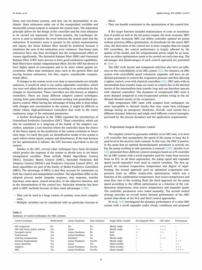
Similar to the GPC, several other techniques have been developedwhich predict the response of the system to decide how to set futuremanipulated variables. These include Model Algorithmic Control(MAC), Dynamic Matrix Control (DMC), Extended Prediction SelfAdaptive Control (EPSAC) and Predictive Function Control (PFC). Allthese algorithms are part of the family of Model Predictive Controllers(MPC). The advantage of MPCs is that they account for constraints onboth the control and manipulated variables. The algorithms differ in theadopted process model (impulse response, step response, transferfunctions, state-space, neural networks), in the objective function, andin the determination of the control law. Particular attention has beenpaid to MPC methods because of their main advantages [108]:

– They can be used in a large variety of systems, even more complexones;

– Multiple variables can be considered with no particular increase in

effort;– They can handle constraints in the optimization of the control law.

If the target function includes minimization of costs or maximiza-tion of profits as well as the net power output, the term economic MPCis often used. Economic MPC can define controller optimal set pointswithout previous offline optimization. As drawbacks for the entire MPCclass, the derivation of the control law is more complex than for simplePID controllers, the control performance is largely affected by thequality of the model, and the computational power might be an issue,since an online optimization needs to be carried out each time step. Theadvantages and disadvantages of each control approach are presentedin Table 3.

The ORC cycle layout and component selection also have an influ-ence on the controllability of an ORC system [83]. For instance, an ORCsystem with controllable speed volumetric expander will have an ad-ditional parameter to control the evaporator pressure and thus allowinga tighter control, even with classical controllers [22]. ORC units with anintermediate heat transfer loops are easier to control due to the thermalinertia of the intermediate heat transfer loop and can therefore operatewith classical controllers. The dynamics of recuperated ORC units ismore damped compared to non-recuperated systems owing to the ad-ditional thermal inertia of the recuperator.

High temperature ORC units with compact heat exchangers aremore susceptible to thermal shocks that may cause heat exchangerdamage during an emergency shutdown. Overall, each system has adifferent dynamic behavior and might need different control strategies,governed by the process dynamics and the application requirements.

3.1. Proportional–integral–derivative control

The simplest control to guarantee stability of an ORC unit, is to havea PI controller that manipulates the speed of the pump to keep the li-quid level in the receiver tank constant. In this way, the ORC is passive,in the sense that no optimal thermodynamic parameter is actively set,but the pump working in safe operation is ensured [108]. Quoilin et al.[22] presented three different control strategies based on a PI controllerfor an ORC system with a scroll expander used for waste heat recoveryfrom an ICE. In all three approaches, the pump speed and expanderspeed (scroll expander) were used as control variables. The first ap-proach set constant evaporation temperature and degree of super-heating; the second approach used an optimized evaporation tem-perature from an offline steady-state optimization, which was afunction of the condensation temperature, heat source temperature andmass flow rate of the working fluid; the third approach set the pumpspeed according to the offline optimization as a function of the con-densation temperature, heat source temperature and expander speed.The controller parameters were tuned manually. The second controlstrategy provides an overall better thermal performance of the ORCsystem than those of the first and third control approaches.

Ni et al. [33] investigated the dynamic performance of a solar ORCsystem with a scroll expander under cloudy conditions and proposed

Table 3Summary of control techniques for ORC systems.

Control technique Model-based Linear/Nonlinear State estimator Single/Multi-variable Development effort CPU effort Performance

PID (empirical) No NA No Mostly single + +++ –PID with linear system analysis Yes Linear No Mostly single ++ +++ –Cascaded control Yes Linear/Nonlinear No Both + ++ +Feed-forward Yes Linear/Nonlinear No Both + + +Lead/lag compensation Yes Nonlinear No Mostly single + +++ +Dynamic Programming Yes Linear/Nonlinear Yes/No Mostly single – – +++Linear Quadratic Yes Linear Yes Multi-variable – + ++Adaptive Yes Linear/Nonlinear Yes/No Multi-variable – — +++MPC Yes Linear/Nonlinear Yes/No Multi-variable – — ++++


15

two conventional proportional–integral–derivative (PID) controllers fortwo control variables. The evaporation pressure and degree of super-heating were controlled by manipulating the pump and expanderspeeds. The set points for both the evaporation pressure and the degreeof superheating were kept constant. The results suggest that the cloudblockage of the sun for short periods (five minutes) does not affect theperformance of the ORC system. For the specified simulation time(5000–30,000 s), the system without the controller generated 84.95kWh, while its counterpart with the PID control strategy generated105.54 kWh, achieving an improvement of 24%.

Luong et al. [109] developed the load-following control strategy foran ORC system that recovers the waste heat of a heavy-duty dieselpowertrain. Three independent PI controllers controlled the evapora-tion pressure, condensing pressure, and the load demand. The massflow rate of the sink fluid and two throttle valves were selected asmanipulated variables. Li et al. [34] developed a dynamic model of asmall-scale solar ORC system with a turbine including a thermal storagesystem. It was observed that for a specific solar period, there is a spe-cific range of thermal storage system capacity that causes instability. Itwas concluded that the capacity of the thermal storage system shouldbe carefully designed based on the local solar irradiation and dynamicresponse of the thermal storage system. A PI controller was used toensure the stable operation of the system by maintaining a constantdegree of superheating by manipulating the pump speed. Lin et al. [95]compared an ORC and an oil storage/ORC system recovering waste heatfrom an automotive internal-combustion engine. PID controllers wereused for the ORC unit, which acted on the speed of the pump and theexpander to control the evaporator pressure and degree of super-heating. The integration of an intermediate oil storage could dampenthe dynamic oscillations, but the costs per unit kW were higher than fora simple ORC unit.

Jolevski et al. [44] developed a control structure of an ORC systembased on the non-square relative gain array and dynamic non-squarerelative gain array methods. A state-space model of the ORC unit wasdeveloped using a moving boundary approach for the heat exchangersand considering a turbine with a control valve as the expander. Thestate-space model has been linearized, so that the coupling between thecontrol variables (the turbine inlet pressure and temperature as well asthe condensation pressure) and the manipulated variables (the massflow rate of the coolant, the rotational speed of the pump and theopening of the turbine throttle valve) were analyzed. Approximatedtransfer functions, obtained from a Bode diagram (graph of the

frequency response of a system), were used to get the optimal para-meters of the control structure. The independent PI controllers weretuned to satisfy the robustness, phase margin of 45°, and high band-width. The proposed structure achieved satisfactory control perfor-mance for constant set points. Marchionni et al. [96] developed a dy-namic model of a 40-kW ORC system with radial turbine and plate heatexchangers and compared four different control strategies. For all cases,the control variable is the turbine inlet temperature, which is kept atthe nominal value, to achieve maximum power output, to avoid thermaldegradation of the working fluid and to keep sufficient superheating atthe turbine inlet. The control strategies differed in the choice of themanipulated variables: (i) speed of the pump only; (ii) speed of theturbine only; (iii) speed of both the pump and the turbine; and (iv)speed of the pump and recirculation from the pump to the condenser. PIcontrollers with anti-windup were chosen and calibrated based on thestep response of the system. The turbine-based regulation strategiesachieved better control performance, whereas the pump-based controlstrategies could keep the net power output closer to the design point forincrease and decrease ramps of the heat source mass flow rate.

Imran et al. [97] developed a PID control strategy for waste heatrecovery from long-haul trucks. The controllers were tested on a 45-minute run of a 450 hp 13 l long-haul truck engine. The control variablefor every case was the degree of superheating at the turbine inlet,whose set point was set to 20 K. The controllers were tuned using thePID tuner application from MATLAB [110]. Two control strategies wereinvestigated with the manipulated variables: (i) the speed of the pumpand a bypass valve for the exhaust gas flow entering the ORC eva-porator; and (ii) the speed of the pump and a throttling valve at theturbine inlet. The second control strategy could increase the net poweroutput and outperform the first one.

Yang et al. [98] focused on a manager/controller structure of anORC recovering waste heat from a vehicle, where the manager has aninternal optimizer that defines the operational mode and optimizes theevaporating and condensing pressures, whereas the controller utilizesPIDs. The performance was simulated on the Highway Fuel EconomyTest cycle. The degree of superheating could be kept within 5–15 K. Incontrast to testing the controller in a simulation environment, Usmanet al. [111] presented the implementation of a PI controller in an ORCunit with a scroll expander. The controller was compared with a PI withfeed-forward and lead-lag compensator on an actual experimental rig.

A FCL strategy was followed, and the speed of the expander was thecontrol variable. The speed of the pump was chosen as the manipulated

Fig. 11. Tracking of the expander set point speed by different control approaches, Usman et al. [111].


16

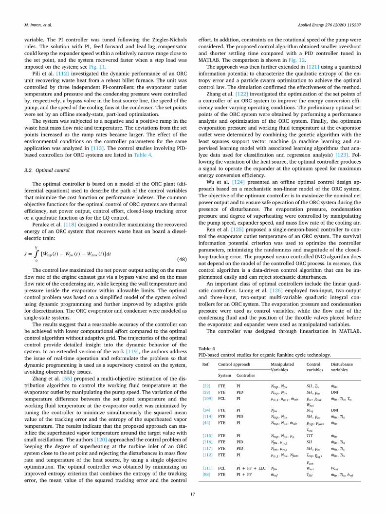
variable. The PI controller was tuned following the Ziegler-Nicholsrules. The solution with PI, feed-forward and lead-lag compensatorcould keep the expander speed within a relatively narrow range close tothe set point, and the system recovered faster when a step load wasimposed on the system; see Fig. 11.

Pili et al. [112] investigated the dynamic performance of an ORCunit recovering waste heat from a reheat billet furnace. The unit wascontrolled by three independent PI-controllers: the evaporator outlettemperature and pressure and the condensing pressure were controlledby, respectively, a bypass valve in the heat source line, the speed of thepump, and the speed of the cooling fans at the condenser. The set pointswere set by an offline steady-state, part-load optimization.

The system was subjected to a negative and a positive ramp in thewaste heat mass flow rate and temperature. The deviations from the setpoints increased as the ramp rates became larger. The effect of theenvironmental conditions on the controller parameters for the sameapplication was analyzed in [113]. The control studies involving PID-based controllers for ORC systems are listed in Table 4.

3.2. Optimal control

The optimal controller is based on a model of the ORC plant (dif-ferential equations) used to describe the path of the control variablesthat minimize the cost function or performance indexes. The commonobjective functions for the optimal control of ORC systems are thermalefficiency, net power output, control effort, closed-loop tracking erroror a quadratic function as for the LQ control.

Peralez et al. [118] designed a controller maximizing the recoveredenergy of an ORC system that recovers waste heat on board a diesel-electric train:

=J W t W t W t dt[ ( ) ( ) ( )]t

exp pu Aux0

f

(48)

The control law maximized the net power output acting on the massflow rate of the engine exhaust gas via a bypass valve and on the massflow rate of the condensing air, while keeping the wall temperature andpressure inside the evaporator within allowable limits. The optimalcontrol problem was based on a simplified model of the system solvedusing dynamic programming and further improved by adaptive gridsfor discretization. The ORC evaporator and condenser were modeled assingle-state systems.

The results suggest that a reasonable accuracy of the controller canbe achieved with lower computational effort compared to the optimalcontrol algorithm without adaptive grid. The trajectories of the optimalcontrol provide detailed insight into the dynamic behavior of thesystem. In an extended version of the work [119], the authors addressthe issue of real-time operation and reformulate the problem so thatdynamic programming is used as a supervisory control on the system,avoiding observability issues.

Zhang et al. [55] proposed a multi-objective estimation of the dis-tribution algorithm to control the working fluid temperature at theevaporator outlet by manipulating the pump speed. The variation of thetemperature difference between the set point temperature and theworking fluid temperature at the evaporator outlet was minimized bytuning the controller to minimize simultaneously the squared meanvalue of the tracking error and the entropy of the superheated vaportemperature. The results indicate that the proposed approach can sta-bilize the superheated vapor temperature around the target value withsmall oscillations. The authors [120] approached the control problem ofkeeping the degree of superheating at the turbine inlet of an ORCsystem close to the set point and rejecting the disturbances in mass flowrate and temperature of the heat source, by using a single objectiveoptimization. The optimal controller was obtained by minimizing animproved entropy criterion that combines the entropy of the trackingerror, the mean value of the squared tracking error and the control

effort. In addition, constraints on the rotational speed of the pump wereconsidered. The proposed control algorithm obtained smaller overshootand shorter settling time compared with a PID controller tuned inMATLAB. The comparison is shown in Fig. 12.

The approach was then further extended in [121] using a quantizedinformation potential to characterize the quadratic entropy of the en-tropy error and a particle swarm optimization to achieve the optimalcontrol law. The simulation confirmed the effectiveness of the method.

Zhang et al. [122] investigated the optimization of the set points ofa controller of an ORC system to improve the energy conversion effi-ciency under varying operating conditions. The preliminary optimal setpoints of the ORC system were obtained by performing a performanceanalysis and optimization of the ORC system. Finally, the optimumevaporation pressure and working fluid temperature at the evaporatoroutlet were determined by combining the genetic algorithm with theleast squares support vector machine (a machine learning and su-pervised learning model with associated learning algorithms that ana-lyze data used for classification and regression analysis) [123]. Fol-lowing the variation of the heat source, the optimal controller producesa signal to operate the expander at the optimum speed for maximumenergy conversion efficiency.

Wu et al. [124] presented an offline optimal control design ap-proach based on a mechanistic non-linear model of the ORC system.The objective of the optimum controller is to maximize the nominal netpower output and to ensure safe operation of the ORC system during thepresence of disturbances. The evaporation pressure, condensationpressure and degree of superheating were controlled by manipulatingthe pump speed, expander speed, and mass flow rate of the cooling air.

Ren et al. [125] proposed a single-neuron-based controller to con-trol the evaporator outlet temperature of an ORC system. The survivalinformation potential criterion was used to optimize the controllerparameters, minimizing the randomness and magnitude of the closed-loop tracking error. The proposed neuro-controlled (NC) algorithm doesnot depend on the model of the controlled ORC process. In essence, thiscontrol algorithm is a data-driven control algorithm that can be im-plemented easily and can reject stochastic disturbances.

An important class of optimal controllers include the linear quad-ratic controllers. Luong et al. [126] employed two-input, two-outputand three-input, two-output multi-variable quadratic integral con-trollers for an ORC system. The evaporation pressure and condensationpressure were used as control variables, while the flow rate of thecondensing fluid and the position of the throttle valves placed beforethe evaporator and expander were used as manipulated variables.

The controller was designed through linearization in MATLAB.

Table 4PID-based control studies for organic Rankine cycle technology.

Ref. Control approach ManipulatedVariables

Controlvariables

Disturbancevariables

System Controller

[22] FTE PI Nexp, Npu SH , Tev mhs[33] FTE PID Nexp, Npu SH , pev DNI[109] FCL PI µ µ m, ,tv tv air,1 ,2 pev, pcon,

Wnet

mhs , Ths , Tss

[34] FTE PI Npu Nexp DNI[114] FTE PID Nexp, Npu SH , pev mhs , Ths[44] FTE PI Nexp, Npu, mair pexp, pcon ,

Texp

mhs

[115] FTE PI Nexp, Npu, µtv TIT mhs[116] FTE PID Npu, µtv,1 SH mhs , Ths

[117] FTE PID Npu, µtv,1 SH , pev mhs , Ths

[112] FTE PI µ N,tv pu,1 , Nfans T p,exp exp,

pcon

mhs , Ths

[111] FCL PI + FF + LLC Npu Wnet Wnet[88] FTE PI + FF mwf TSH mhs , Ths , hwf


17

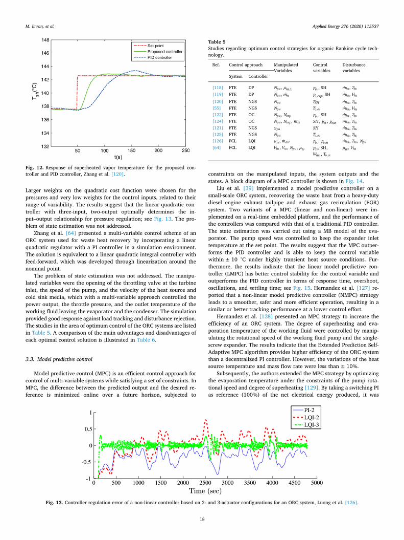
Larger weights on the quadratic cost function were chosen for thepressures and very low weights for the control inputs, related to theirrange of variability. The results suggest that the linear quadratic con-troller with three-input, two-output optimally determines the in-put–output relationship for pressure regulation; see Fig. 13. The pro-blem of state estimation was not addressed.

Zhang et al. [64] presented a multi-variable control scheme of anORC system used for waste heat recovery by incorporating a linearquadratic regulator with a PI controller in a simulation environment.The solution is equivalent to a linear quadratic integral controller withfeed-forward, which was developed through linearization around thenominal point.

The problem of state estimation was not addressed. The manipu-lated variables were the opening of the throttling valve at the turbineinlet, the speed of the pump, and the velocity of the heat source andcold sink media, which with a multi-variable approach controlled thepower output, the throttle pressure, and the outlet temperature of theworking fluid leaving the evaporator and the condenser. The simulationprovided good response against load tracking and disturbance rejection.The studies in the area of optimum control of the ORC systems are listedin Table 5. A comparison of the main advantages and disadvantages ofeach optimal control solution is illustrated in Table 6.

3.3. Model predictive control

Model predictive control (MPC) is an efficient control approach forcontrol of multi-variable systems while satisfying a set of constraints. InMPC, the difference between the predicted output and the desired re-ference is minimized online over a future horizon, subjected to

constraints on the manipulated inputs, the system outputs and thestates. A block diagram of a MPC controller is shown in Fig. 14.

Liu et al. [39] implemented a model predictive controller on asmall-scale ORC system, recovering the waste heat from a heavy-dutydiesel engine exhaust tailpipe and exhaust gas recirculation (EGR)system. Two variants of a MPC (linear and non-linear) were im-plemented on a real-time embedded platform, and the performance ofthe controllers was compared with that of a traditional PID controller.The state estimation was carried out using a MB model of the eva-porator. The pump speed was controlled to keep the expander inlettemperature at the set point. The results suggest that the MPC outper-forms the PID controller and is able to keep the control variablewithin± 10 °C under highly transient heat source conditions. Fur-thermore, the results indicate that the linear model predictive con-troller (LMPC) has better control stability for the control variable andoutperforms the PID controller in terms of response time, overshoot,oscillations, and settling time; see Fig. 15. Hernandez et al. [127] re-ported that a non-linear model predictive controller (NMPC) strategyleads to a smoother, safer and more efficient operation, resulting in asimilar or better tracking performance at a lower control effort.

Hernandez et al. [128] presented an MPC strategy to increase theefficiency of an ORC system. The degree of superheating and eva-poration temperature of the working fluid were controlled by manip-ulating the rotational speed of the working fluid pump and the single-screw expander. The results indicate that the Extended Prediction Self-Adaptive MPC algorithm provides higher efficiency of the ORC systemthan a decentralized PI controller. However, the variations of the heatsource temperature and mass flow rate were less than± 10%.

Subsequently, the authors extended the MPC strategy by optimizingthe evaporation temperature under the constraints of the pump rota-tional speed and degree of superheating [129]. By taking a switching PIas reference (100%) of the net electrical energy produced, it was

Fig. 12. Response of superheated vapor temperature for the proposed con-troller and PID controller, Zhang et al. [120].

Fig. 13. Controller regulation error of a non-linear controller based on 2- and 3-actuator configurations for an ORC system, Luong et al. [126].

Table 5Studies regarding optimum control strategies for organic Rankine cycle tech-nology.

Ref. Control approach ManipulatedVariables

Controlvariables


System Controller

[118] FTE DP Npu, µhs,1 pev, SH mhs , Ths

[119] FTE DP Npu, mss pi exp, , SH mhs , Vhs

[120] FTE NGS Npu TSH mhs , Ths[55] FTE NGS Npu To ev, mhs , Vhs[122] FTE OC Npu, Nexp pev, SH mhs , Ths[124] FTE OC Npu, Nexp, mss SH , pev, pcon mhs , Ths[121] FTE NGS pu SH mhs , Ths[125] FTE NGS Npu To ev, mhs , Ths[126] FCL LQI µtv, mair pev, pcon mhs , Ths, Npu[64] FCL LQI Vhs , Vss, Npu, µtv ptv, SH,

Wnet , To co,

µ V,tv hs


18

concluded that the basic MPC produces 15% more energy, as it requiresless control effort while keeping the unit in safe operation. The highernet power output is obtained by accurately optimizing the evaporationtemperature, while keeping the degree of superheating within safelimits. However, the controller was evaluated for only± 10% variationof the heat source temperature and the mass flow rate.

Zhang et al. [130] presented a multiple MPC approach to deal withthe non-linearity and varying operating conditions of ORC systemsutilizing a transient heat source. The rotational speed of the pump andthe shaft torque of the expander were manipulated simultaneously toprovide the optimal evaporating pressure and superheating tempera-ture. The operating range of the ORC system was divided into sub-op-erating regions, and the system response was represented by a CARIMAmodel. The predicted outputs of all sub-models and their correspondingweights were used to obtain the control signal. The simulation resultssuggest that the multiple MPC approach can effectively deal with non-linearity, constraints on the control variables, manipulated variablesand varying operating points.

Pierobon et al. [131] implemented a linear MPC for offshore powerstations with waste heat recovery using an ORC system. The MPC wascoupled with a steady-state performance optimizer developed in SIM-ULINK/MATLAB [110]. The pump speed was varied to control thedegree of superheating at turbine inlet. Transfer functions were

Table 6Advantages and disadvantages of optimal control strategies for organic Rankine cycle technology.

Controller Advantages Disadvantages

Dynamic Programming • Applicable to both linear and non-linear systems

• Real-time optimization of plant trajectory• High computational effort

• Multi-variable approach, highly computationallyexpensive

Non-Gaussian stochastic control (minimum entropycriterion)

• Minimizes uncertainties in tracking error

• Real-time optimization of control inputs

• Multi-variable control possible

• Real-time multi-objective optimization required

Data-driven set point optimization • Allows for real-time optimization of plant trajectory

• Adaptive algorithm can account for system aging andsmall variations

• Training of estimating function, computationallyexpensive

• Large data-set required for good accuracy

• System modifications require new training

Linear quadratic control • Simple, fast and robust algorithm

• Can handle high order systems and multi-variablecontrol

• Requires system linearization

• Weight matrices need to be chosen properly

Fig. 14. Basic structure of the model predictive controller, Liu et al. [39].

Fig. 15. Temperature responses of LMPC and PID controllers for a step changein set point temperature and engine operating conditions, adapted from Liuet al. [39].


19

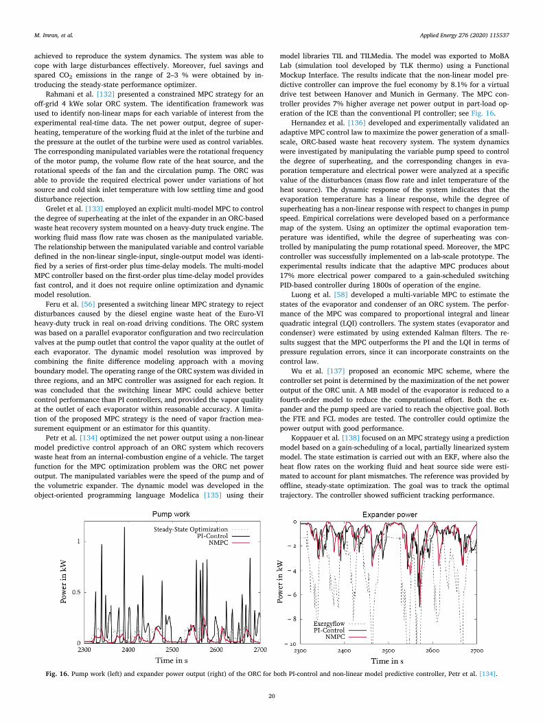
achieved to reproduce the system dynamics. The system was able tocope with large disturbances effectively. Moreover, fuel savings andspared CO2 emissions in the range of 2–3 % were obtained by in-troducing the steady-state performance optimizer.

Rahmani et al. [132] presented a constrained MPC strategy for anoff-grid 4 kWe solar ORC system. The identification framework wasused to identify non-linear maps for each variable of interest from theexperimental real-time data. The net power output, degree of super-heating, temperature of the working fluid at the inlet of the turbine andthe pressure at the outlet of the turbine were used as control variables.The corresponding manipulated variables were the rotational frequencyof the motor pump, the volume flow rate of the heat source, and therotational speeds of the fan and the circulation pump. The ORC wasable to provide the required electrical power under variations of hotsource and cold sink inlet temperature with low settling time and gooddisturbance rejection.

Grelet et al. [133] employed an explicit multi-model MPC to controlthe degree of superheating at the inlet of the expander in an ORC-basedwaste heat recovery system mounted on a heavy-duty truck engine. Theworking fluid mass flow rate was chosen as the manipulated variable.The relationship between the manipulated variable and control variabledefined in the non-linear single-input, single-output model was identi-fied by a series of first-order plus time-delay models. The multi-modelMPC controller based on the first-order plus time-delay model providesfast control, and it does not require online optimization and dynamicmodel resolution.

Feru et al. [56] presented a switching linear MPC strategy to rejectdisturbances caused by the diesel engine waste heat of the Euro-VIheavy-duty truck in real on-road driving conditions. The ORC systemwas based on a parallel evaporator configuration and two recirculationvalves at the pump outlet that control the vapor quality at the outlet ofeach evaporator. The dynamic model resolution was improved bycombining the finite difference modeling approach with a movingboundary model. The operating range of the ORC system was divided inthree regions, and an MPC controller was assigned for each region. Itwas concluded that the switching linear MPC could achieve bettercontrol performance than PI controllers, and provided the vapor qualityat the outlet of each evaporator within reasonable accuracy. A limita-tion of the proposed MPC strategy is the need of vapor fraction mea-surement equipment or an estimator for this quantity.

Petr et al. [134] optimized the net power output using a non-linearmodel predictive control approach of an ORC system which recoverswaste heat from an internal-combustion engine of a vehicle. The targetfunction for the MPC optimization problem was the ORC net poweroutput. The manipulated variables were the speed of the pump and ofthe volumetric expander. The dynamic model was developed in theobject-oriented programming language Modelica [135] using their

model libraries TIL and TILMedia. The model was exported to MoBALab (simulation tool developed by TLK thermo) using a FunctionalMockup Interface. The results indicate that the non-linear model pre-dictive controller can improve the fuel economy by 8.1% for a virtualdrive test between Hanover and Munich in Germany. The MPC con-troller provides 7% higher average net power output in part-load op-eration of the ICE than the conventional PI controller; see Fig. 16.

Hernandez et al. [136] developed and experimentally validated anadaptive MPC control law to maximize the power generation of a small-scale, ORC-based waste heat recovery system. The system dynamicswere investigated by manipulating the variable pump speed to controlthe degree of superheating, and the corresponding changes in eva-poration temperature and electrical power were analyzed at a specificvalue of the disturbances (mass flow rate and inlet temperature of theheat source). The dynamic response of the system indicates that theevaporation temperature has a linear response, while the degree ofsuperheating has a non-linear response with respect to changes in pumpspeed. Empirical correlations were developed based on a performancemap of the system. Using an optimizer the optimal evaporation tem-perature was identified, while the degree of superheating was con-trolled by manipulating the pump rotational speed. Moreover, the MPCcontroller was successfully implemented on a lab-scale prototype. Theexperimental results indicate that the adaptive MPC produces about17% more electrical power compared to a gain-scheduled switchingPID-based controller during 1800s of operation of the engine.

Luong et al. [58] developed a multi-variable MPC to estimate thestates of the evaporator and condenser of an ORC system. The perfor-mance of the MPC was compared to proportional integral and linearquadratic integral (LQI) controllers. The system states (evaporator andcondenser) were estimated by using extended Kalman filters. The re-sults suggest that the MPC outperforms the PI and the LQI in terms ofpressure regulation errors, since it can incorporate constraints on thecontrol law.

Wu et al. [137] proposed an economic MPC scheme, where thecontroller set point is determined by the maximization of the net poweroutput of the ORC unit. A MB model of the evaporator is reduced to afourth-order model to reduce the computational effort. Both the ex-pander and the pump speed are varied to reach the objective goal. Boththe FTE and FCL modes are tested. The controller could optimize thepower output with good performance.

Koppauer et al. [138] focused on an MPC strategy using a predictionmodel based on a gain-scheduling of a local, partially linearized systemmodel. The state estimation is carried out with an EKF, where also theheat flow rates on the working fluid and heat source side were esti-mated to account for plant mismatches. The reference was provided byoffline, steady-state optimization. The goal was to track the optimaltrajectory. The controller showed sufficient tracking performance.

Fig. 16. Pump work (left) and expander power output (right) of the ORC for both PI-control and non-linear model predictive controller, Petr et al. [134].


20

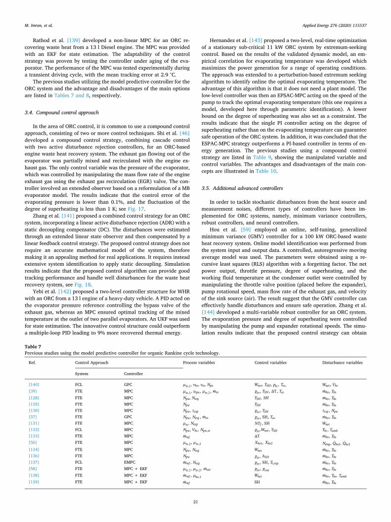
Rathod et al. [139] developed a non-linear MPC for an ORC re-covering waste heat from a 13 l Diesel engine. The MPC was providedwith an EKF for state estimation. The adaptability of the controlstrategy was proven by testing the controller under aging of the eva-porator. The performance of the MPC was tested experimentally duringa transient driving cycle, with the mean tracking error at 2.9 °C.

The previous studies utilizing the model predictive controller for theORC system and the advantage and disadvantages of the main optionsare listed in Tables 7 and 8, respectively.

3.4. Compound control approach

In the area of ORC control, it is common to use a compound controlapproach, consisting of two or more control techniques. Shi et al. [46]developed a compound control strategy, combining cascade controlwith two active disturbance rejection controllers, for an ORC-basedengine waste heat recovery system. The exhaust gas flowing out of theevaporator was partially mixed and recirculated with the engine ex-haust gas. The only control variable was the pressure of the evaporator,which was controlled by manipulating the mass flow rate of the engineexhaust gas using the exhaust gas recirculation (EGR) valve. The con-troller involved an extended observer based on a reformulation of a MBevaporator model. The results indicate that the control error of theevaporating pressure is lower than 0.1%, and the fluctuation of thedegree of superheating is less than 1 K; see Fig. 17.

Zhang et al. [141] proposed a combined control strategy for an ORCsystem, incorporating a linear active disturbance rejection (ADR) with astatic decoupling compensator (DC). The disturbances were estimatedthrough an extended linear state observer and then compensated by alinear feedback control strategy. The proposed control strategy does notrequire an accurate mathematical model of the system, thereforemaking it an appealing method for real applications. It requires insteadextensive system identification to apply static decoupling. Simulationresults indicate that the proposed control algorithm can provide goodtracking performance and handle well disturbances for the waste heatrecovery system, see Fig. 18.

Yebi et al. [142] proposed a two-level controller structure for WHRwith an ORC from a 13 l engine of a heavy-duty vehicle. A PID acted onthe evaporator pressure reference controlling the bypass valve of theexhaust gas, whereas an MPC ensured optimal tracking of the mixedtemperature at the outlet of two parallel evaporators. An UKF was usedfor state estimation. The innovative control structure could outperforma multiple-loop PID leading to 9% more recovered thermal energy.

Hernandez et al. [143] proposed a two-level, real-time optimizationof a stationary sub-critical 11 kW ORC system by extremum-seekingcontrol. Based on the results of the validated dynamic model, an em-pirical correlation for evaporating temperature was developed whichmaximizes the power generation for a range of operating conditions.The approach was extended to a perturbation-based extremum seekingalgorithm to identify online the optimal evaporating temperature. Theadvantage of this algorithm is that it does not need a plant model. Thelow-level controller was then an EPSAC-MPC acting on the speed of thepump to track the optimal evaporating temperature (this one requires amodel, developed here through parametric identification). A lowerbound on the degree of superheating was also set as a constraint. Theresults indicate that the single PI controller acting on the degree ofsuperheating rather than on the evaporating temperature can guaranteesafe operation of the ORC system. In addition, it was concluded that theESPAC-MPC strategy outperforms a PI-based controller in terms of en-ergy generation. The previous studies using a compound controlstrategy are listed in Table 9, showing the manipulated variable andcontrol variables. The advantages and disadvantages of the main con-cepts are illustrated in Table 10.

3.5. Additional advanced controllers

In order to tackle stochastic disturbances from the heat source andmeasurement noises, different types of controllers have been im-plemented for ORC systems, namely, minimum variance controllers,robust controllers, and neural controllers.

Hou et al. [59] employed an online, self-tuning, generalizedminimum variance (GMV) controller for a 100 kW ORC-based wasteheat recovery system. Online model identification was performed fromthe system input and output data. A controlled, autoregressive movingaverage model was used. The parameters were obtained using a re-cursive least squares (RLS) algorithm with a forgetting factor. The netpower output, throttle pressure, degree of superheating, and theworking fluid temperature at the condenser outlet were controlled bymanipulating the throttle valve position (placed before the expander),pump rotational speed, mass flow rate of the exhaust gas, and velocityof the sink source (air). The result suggest that the GMV controller caneffectively handle disturbances and ensure safe operation. Zhang et al.[144] developed a multi-variable robust controller for an ORC system.The evaporation pressure and degree of superheating were controlledby manipulating the pump and expander rotational speeds. The simu-lation results indicate that the proposed control strategy can obtain

Table 7Previous studies using the model predictive controller for organic Rankine cycle technology.

Ref. Control Approach Process variables Control variables Disturbance variables

System Controller

[140] FCL GPC µ v v N, , ,tv hs ss pu,1 W T p T, , ,net SH tv co, Wnet , Vhs

[39] FTE MPC µ ,tv pu,1 , µtv,2, mss pev, TSH , T, Tco mhs , Ths

[128] FTE MPC N N,pu exp T SH,SH mhs , Ths[129] FTE MPC Npu TSH mhs , Ths[130] FTE MPC Npu, exp pev, TSH exp, Npu[57] FTE GPC Npu, Nexp, mss pev, SH, Tco mhs , Ths[131] FTE MPC µ N,tv exp NTf , SH Wnet[132] FCL MPC Npu, Vhs, Npu ss, p W,ev net , TSH Ths, Tamb[133] FTE MPC mwf T mhs , Ths[56] FTE MPC µtv,1, µtv,2 Xhs1, Xhs2 Neng , Qhs1, Qhs2[134] FTE MPC Npu, Nexp Wnet mhs , Ths[136] FTE MPC Npu p h,ev SH mhs , Ths[137] FCL EMPC m N,wf exp pev, SH, Ti exp, mhs , Ths[58] FTE MPC + EKF µ µ m, ,tv tv air,1 ,2 pev, pcon mhs , Ths

[138] FTE MPC + EKF mwf , µhs,1 Wnet mhs , T T,hs amb

[139] FTE MPC + EKF mwf SH mhs , Ths


21

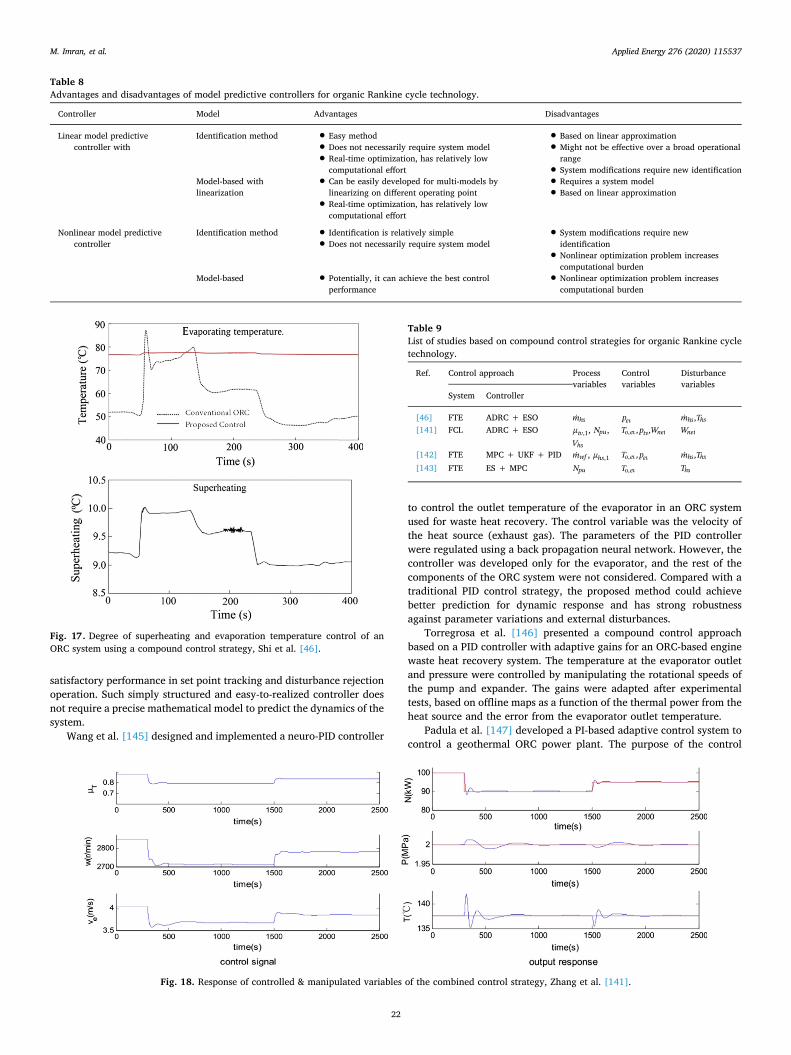
satisfactory performance in set point tracking and disturbance rejectionoperation. Such simply structured and easy-to-realized controller doesnot require a precise mathematical model to predict the dynamics of thesystem.

Wang et al. [145] designed and implemented a neuro-PID controller

to control the outlet temperature of the evaporator in an ORC systemused for waste heat recovery. The control variable was the velocity ofthe heat source (exhaust gas). The parameters of the PID controllerwere regulated using a back propagation neural network. However, thecontroller was developed only for the evaporator, and the rest of thecomponents of the ORC system were not considered. Compared with atraditional PID control strategy, the proposed method could achievebetter prediction for dynamic response and has strong robustnessagainst parameter variations and external disturbances.

Torregrosa et al. [146] presented a compound control approachbased on a PID controller with adaptive gains for an ORC-based enginewaste heat recovery system. The temperature at the evaporator outletand pressure were controlled by manipulating the rotational speeds ofthe pump and expander. The gains were adapted after experimentaltests, based on offline maps as a function of the thermal power from theheat source and the error from the evaporator outlet temperature.

Padula et al. [147] developed a PI-based adaptive control system tocontrol a geothermal ORC power plant. The purpose of the control

Table 8Advantages and disadvantages of model predictive controllers for organic Rankine cycle technology.

Controller Model Advantages Disadvantages

Linear model predictivecontroller with

Identification method • Easy method

• Does not necessarily require system model

• Real-time optimization, has relatively lowcomputational effort

• Based on linear approximation

• Might not be effective over a broad operationalrange

• System modifications require new identificationModel-based withlinearization

• Can be easily developed for multi-models bylinearizing on different operating point

• Real-time optimization, has relatively lowcomputational effort

• Requires a system model

• Based on linear approximation

Nonlinear model predictivecontroller

Identification method • Identification is relatively simple

• Does not necessarily require system model• System modifications require newidentification

• Nonlinear optimization problem increasescomputational burden

Model-based • Potentially, it can achieve the best controlperformance

• Nonlinear optimization problem increasescomputational burden

Fig. 17. Degree of superheating and evaporation temperature control of anORC system using a compound control strategy, Shi et al. [46].

Fig. 18. Response of controlled & manipulated variables of the combined control strategy, Zhang et al. [141].

Table 9List of studies based on compound control strategies for organic Rankine cycletechnology.

Ref. Control approach Processvariables

Controlvariables


System Controller

[46] FTE ADRC + ESO mhs pev mhs ,Ths[141] FCL ADRC + ESO µtv,1, Npu,

Vhs

To ev, ,ptv,Wnet Wnet

[142] FTE MPC + UKF + PID mwf , µhs,1 To ev, ,pev mhs ,Ths

[143] FTE ES + MPC Npu To ev, Ths


22

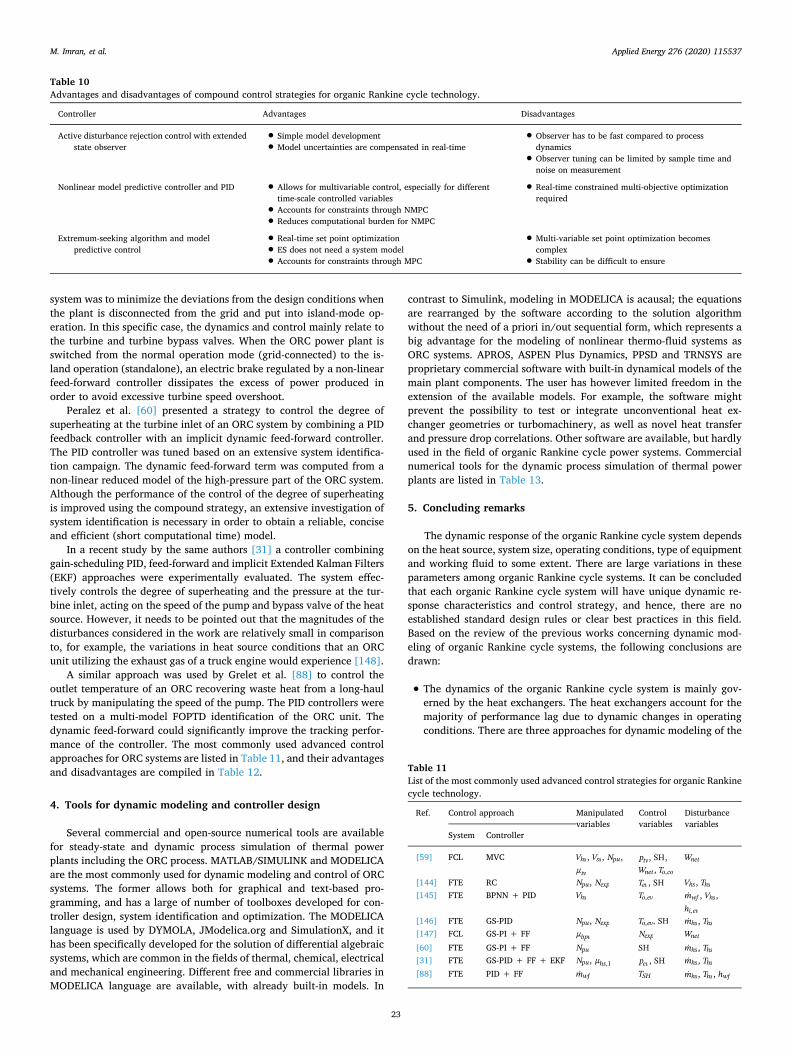
system was to minimize the deviations from the design conditions whenthe plant is disconnected from the grid and put into island-mode op-eration. In this specific case, the dynamics and control mainly relate tothe turbine and turbine bypass valves. When the ORC power plant isswitched from the normal operation mode (grid-connected) to the is-land operation (standalone), an electric brake regulated by a non-linearfeed-forward controller dissipates the excess of power produced inorder to avoid excessive turbine speed overshoot.

Peralez et al. [60] presented a strategy to control the degree ofsuperheating at the turbine inlet of an ORC system by combining a PIDfeedback controller with an implicit dynamic feed-forward controller.The PID controller was tuned based on an extensive system identifica-tion campaign. The dynamic feed-forward term was computed from anon-linear reduced model of the high-pressure part of the ORC system.Although the performance of the control of the degree of superheatingis improved using the compound strategy, an extensive investigation ofsystem identification is necessary in order to obtain a reliable, conciseand efficient (short computational time) model.

In a recent study by the same authors [31] a controller combininggain-scheduling PID, feed-forward and implicit Extended Kalman Filters(EKF) approaches were experimentally evaluated. The system effec-tively controls the degree of superheating and the pressure at the tur-bine inlet, acting on the speed of the pump and bypass valve of the heatsource. However, it needs to be pointed out that the magnitudes of thedisturbances considered in the work are relatively small in comparisonto, for example, the variations in heat source conditions that an ORCunit utilizing the exhaust gas of a truck engine would experience [148].

A similar approach was used by Grelet et al. [88] to control theoutlet temperature of an ORC recovering waste heat from a long-haultruck by manipulating the speed of the pump. The PID controllers weretested on a multi-model FOPTD identification of the ORC unit. Thedynamic feed-forward could significantly improve the tracking perfor-mance of the controller. The most commonly used advanced controlapproaches for ORC systems are listed in Table 11, and their advantagesand disadvantages are compiled in Table 12.

4. Tools for dynamic modeling and controller design

Several commercial and open-source numerical tools are availablefor steady-state and dynamic process simulation of thermal powerplants including the ORC process. MATLAB/SIMULINK and MODELICAare the most commonly used for dynamic modeling and control of ORCsystems. The former allows both for graphical and text-based pro-gramming, and has a large of number of toolboxes developed for con-troller design, system identification and optimization. The MODELICAlanguage is used by DYMOLA, JModelica.org and SimulationX, and ithas been specifically developed for the solution of differential algebraicsystems, which are common in the fields of thermal, chemical, electricaland mechanical engineering. Different free and commercial libraries inMODELICA language are available, with already built-in models. In

contrast to Simulink, modeling in MODELICA is acausal; the equationsare rearranged by the software according to the solution algorithmwithout the need of a priori in/out sequential form, which represents abig advantage for the modeling of nonlinear thermo-fluid systems asORC systems. APROS, ASPEN Plus Dynamics, PPSD and TRNSYS areproprietary commercial software with built-in dynamical models of themain plant components. The user has however limited freedom in theextension of the available models. For example, the software mightprevent the possibility to test or integrate unconventional heat ex-changer geometries or turbomachinery, as well as novel heat transferand pressure drop correlations. Other software are available, but hardlyused in the field of organic Rankine cycle power systems. Commercialnumerical tools for the dynamic process simulation of thermal powerplants are listed in Table 13.

5. Concluding remarks

The dynamic response of the organic Rankine cycle system dependson the heat source, system size, operating conditions, type of equipmentand working fluid to some extent. There are large variations in theseparameters among organic Rankine cycle systems. It can be concludedthat each organic Rankine cycle system will have unique dynamic re-sponse characteristics and control strategy, and hence, there are noestablished standard design rules or clear best practices in this field.Based on the review of the previous works concerning dynamic mod-eling of organic Rankine cycle systems, the following conclusions aredrawn:

• The dynamics of the organic Rankine cycle system is mainly gov-erned by the heat exchangers. The heat exchangers account for themajority of performance lag due to dynamic changes in operatingconditions. There are three approaches for dynamic modeling of the

Table 10Advantages and disadvantages of compound control strategies for organic Rankine cycle technology.


Active disturbance rejection control with extendedstate observer

• Simple model development

• Model uncertainties are compensated in real-time• Observer has to be fast compared to processdynamics

• Observer tuning can be limited by sample time andnoise on measurement

Nonlinear model predictive controller and PID • Allows for multivariable control, especially for differenttime-scale controlled variables

• Accounts for constraints through NMPC

• Reduces computational burden for NMPC

• Real-time constrained multi-objective optimizationrequired

Extremum-seeking algorithm and modelpredictive control

• Real-time set point optimization

• ES does not need a system model

• Accounts for constraints through MPC

• Multi-variable set point optimization becomescomplex

• Stability can be difficult to ensure

Table 11List of the most commonly used advanced control strategies for organic Rankinecycle technology.

Ref. Control approach Manipulatedvariables

Controlvariables


System Controller

[59] FCL MVC Vhs , Vss, Npu,µtv

ptv, SH,Wnet , To co,

Wnet

[144] FTE RC Npu, Nexp Tev , SH Vhs , Ths[145] FTE BPNN + PID Vhs To ev, mwf , Vhs,

hi ev,[146] FTE GS-PID Npu, Nexp T , SHo ev, mhs , Ths[147] FCL GS-PI + FF µbpv Nexp Wnet

[60] FTE GS-PI + FF Npu SH mhs , Ths[31] FTE GS-PID + FF + EKF Npu, µhs,1 pev, SH mhs , Ths

[88] FTE PID + FF mwf TSH mhs , Ths , hwf


23

evaporator and condenser of the organic Rankine cycle system,namely, moving boundary, finite volume and two-volume models.The moving boundary approach has lower computational time, buthigher prediction error compared to those of the finite volume ap-proach. However, the computational time of the finite volumemethod can be reduced by selecting an optimum level of dis-cretization. The two-volume approach is applicable only for phasechange in a shell. The addition of the heat transfer and pressure dropcorrelations results in a larger computational effort and higher ac-curacy. The time constants characterizing the expansion and com-pression processes are small compared to those of the evaporatorand condenser. Thus, the expander and pump models are typicallybased on steady-state, lumped parameter models. If performancemaps of these components are available, non-dimensional para-meters can be used to predict their performances. The dynamiccharacteristics of control valves are typically modeled with relevantequations that correlate the valve opening, boundary conditions andthe flow through the component. If the system dynamics are fast, thevalve positioning servo-system plays an important role to determinethe closed-loop dynamic behavior of the system and should there-fore be included in the model. However, it is difficult to gain accessto the information about the servo-positioner dynamics; hence, first-order or second-order linear systems can be used to consider thesedynamics. If experimental data are available, an empirical correla-tion can be developed to calculate the mass flow rate for in-compressible flow (or the equivalent) based on the relative valveopening.• Measuring instruments may have a significant delayed response,especially temperature sensors. If the time-scale of a given mea-suring instrument is not negligible compared to the closed-loop

response time, the response time of the measuring instrumentshould be included in the dynamic model.• Dynamic models have been matched to experimental data withreasonable accuracy. In most of the cases, the relative deviation isdifferent among the observed parameters. For instance, the turbineinlet temperature may have a different relative deviation than thecondenser pressure of the same system in dynamic operation.Previous work indicate that if the models are calibrated properly,dynamic models can predict the process variables within a 3% re-lative deviation from the experimental results.

The control of the organic Rankine cycle systems plays an importantrole in terms of the system performance and safe operation. In thispaper, different control techniques and findings of previous researchwork in the area of control systems of organic Rankine cycle systemswere reviewed and discussed. The prospects and constraints of thedifferent control techniques and their limitations were analyzed anddiscussed. Some important points concerning the development of con-trollers for organic Rankine cycle systems can be summarized as fol-lows:

• The complexity of the control system and corresponding controlstrategy depends on the operation (grid-connected or off-grid) of theorganic Rankine cycle system.• The model predictive controller, especially improved model pre-dictive control (multiple model predictive control, switching modelpredictive control, non-linear model predictive control), providesexcellent control performance as it can deal with non-linearity,process constraints, and a wide range of system disturbances effi-ciently.

Table 12Advantages and disadvantages of the most commonly used advanced control strategies for organic Rankine cycle technology.


Generalized minimum variance • Simple control law

• Can reject stochastic disturbances• Response might be aggressive

• Does not consider input effort in control law

Robust control • Simple control law

• Robust against uncertainties• Based on system linear approximation

• Strict mathematical conditions have to apply

Neuro-PID • Does not require system model

• Can provide online tuning of PID• Quality of training set affects controller performance

• System modifications require new training

Gain-scheduled PI or PID • Good handling of nonlinearities of the system • Scheduling variable has to be chosen carefully to guarantee stability and goodperformance

Feedforward • Good disturbance rejection

• Good set point tracking• Requires system to be non-minimum phase or approximation necessary

• Feedback might be required to account for uncertainties

Table 13List of commercial software for dynamic modeling and control of thermal power plants, from Alobaid et al. [70].

No. Program Developer Website

1 APROS Technical Research Center of Finland http://www.apros.fi/en2 ASPEN Plus Dynamics Aspen Technology, Inc. https://www.aspentech.com3 DYMOLA Dassault Systèmes http://www.3ds.com4 gPROMS Platform Process Systems Enterprise Limited http://www.psenterprise.com5 JModelica.org Modelon AB http://www.jmodelica.org/6 MATHEMATICA Wolfram Research https://www.wolfram.com/mathematica7 SIMULINK The MathWorks, Inc. https://www.mathworks.com8 PPSD KED GmbH http://www.ked.de/index.html?&L=19 ProTRAX Software TRAX Energy Solutions https://energy.traxintl.com10 EASY5, etc. MSC Software http://www.mscsoftware.com11 EcosimPro, PROOSIS. Empresarios Agrupados A.I.E http://www.ecosimpro.com12 SimSci, DYNSIM Schneider Electric Software http://software.schneider-electric.com13 SimulationX ITI GmbH https://www.simulationx.com14 RELAP Idaho National Laboratory http://energy.gov15 TRNSYS University of Wisconsin http://sel.me.wisc.edu/trnsys16 UniSim Design Honeywell https://www.honeywellprocess.com17 3-Key Master Western Services Corporation https://www.ws-corp.com


24

http://www.apros.fi/en

https://www.aspentech.com

http://www.3ds.com

http://www.psenterprise.com

http://www.jmodelica.org/

https://www.wolfram.com/mathematica

https://www.mathworks.com

http://www.ked.de/index.html%3f%26L%3d1

https://energy.traxintl.com

http://www.mscsoftware.com

http://www.ecosimpro.com

http://software.schneider-electric.com

https://www.simulationx.com

http://energy.gov

http://sel.me.wisc.edu/trnsys

https://www.honeywellprocess.com

https://www.ws-corp.com

• Although the control strategies proposed for organic Rankine cyclesystems depend on the dynamic model of the system, a few authorspresented control-oriented models, such as two-state models [119],simplified physical models [22,149], first-order plus dead-timemodel [150], and the transfer functions-based model [128].• There exists an optimal rotational speed for an expander that cor-responds to its maximum isentropic efficiency for specific operatingconditions. It is necessary to investigate both the machine-side andgrid-side controller for organic Rankine cycle power generationsystems. For optimal operation of organic Rankine cycle systems,the use of a supervisory control strategy could be helpful to produceoptimal set points for the control system.• Since the dynamic response of the organic Rankine cycle system iscomplex in terms of non-linearity, coupling and time variation dis-turbances, the use of advanced control algorithms is helpful.• Organic Rankine cycle systems are extremely diversified in terms ofapplications, operating conditions, size, and type of equipment;therefore, the optimal control strategy may be different for eachsystem. In order to identify the optimal control strategy for a givensystem, a comparative analysis of the performance of differentcontrol strategies based on system performance, tracking error,overshoot, rise time, settling time, peak time, robustness to dis-turbances, handling constraints, computational effort, and practicalimplementation needs to be conducted.• Almost all of the previous studies analyzed the performance of thecontroller under a range of variation of the input disturbances ty-pically smaller than those occurring during operation of organicRankine cycle systems utilizing highly transient heat sources inpractice. In order to adapt to fluctuations in the heat sources orconnected load, the performance of the controller needs to beevaluated over a wide (or entire) operating range of the system,ensuring safe and optimal operation of the organic Rankine cyclesystem.

As far as recommendations for future research are concerned, first itneeds to be stressed that in almost all of the previous works, the designand component sizing of the organic Rankine cycle system were basedon the heat sink and heat source conditions without taking into accountthe dynamic response and control of the system. Such design and op-timization approach may lead to an organic Rankine cycle system thatis sensitive to highly transient heat sources and difficult to operate in asafe and efficient manner. Therefore, for future research and designpractice of organic Rankine cycle systems utilizing highly fluctuatingheat sources, we recommend to include the dynamic response andcontrol aspects into the preliminary design of the system in an iterativemanner. Such approach will discard the designs that feature un-acceptable dynamic performance in an early phase of the design processand will support the selection of the best possible combination of on-design, off-design, and dynamic performances, while fulfilling at thesame time all the constraints in terms of the operational parameters ofthe system.

Most of the experimental work discussed the experimental valida-tion of dynamic models which involved matching of response time andsteady-state error for a measured/known disturbance. There are limitedworks which compared the efficacy of different types of controllers.There is an urgent need to implement the proposed controller on a realORC system and assess the performance of the controller under chan-ging heat source or sink conditions. Besides, it is essential to test thedifferent control strategies on the same test rig under the same dis-turbance for a fair comparison of the different control schemes.

The start-up and shut-down control methods had not been reportedin open literature yet, except few patents. The start-up and shut-downcontrol methods for transient heat source are critical and require ad-ditional safety measures. There is a need for implementation to in-vestigate control narratives, which discuss start-up and shut down toensure safe operation and avoid thermal shocks.

Declaration of Competing Interest

The authors declare that they have no known competing financialinterests or personal relationships that could have appeared to influ-ence the work reported in this paper.

Acknowledgement

The research presented in this paper has received funding from theEuropean Union's Horizon 2020 research and innovation programmewith a Marie Skłodowska-Curie Fellowship under grant agreementnumber 751947 (project DYNCON-ORC), as well as the grant agree-ment number 754462 (EuroTechPostdoc, project ACT-ORC). The fi-nancial support is gratefully acknowledged.

References

[1] Colonna P, Casati E, Trapp C, Mathijssen T, Larjola J, Turunen-Saaresti T, et al.Organic rankine cycle power systems: from the concept to current technology,applications, and an outlook to the future. J Eng Gas Turbines Power2015;137:100801. https://doi.org/10.1115/1.4029884.

[2] Forman C, Muritala IK, Pardemann R, Meyer B. Estimating the global waste heatpotential. Renew Sustain Energy Rev 2016;57:1568–79. https://doi.org/10.1016/j.rser.2015.12.192.

[3] Imran M, Park B-S, Kim H-J, Lee D-H, Usman M. Economic assessment of green-house gas reduction through low-grade waste heat recovery using organic Rankinecycle (ORC). J Mech Sci Technol 2015;29:835–43. https://doi.org/10.1007/s12206-015-0147-5.

[4] Tchanche BF, Lambrinos G, Frangoudakis A, Papadakis G. Low-grade heat con-version into power using organic Rankine cycles – A review of various applications.Renew Sustain Energy Rev 2011;15:3963–79. https://doi.org/10.1016/j.rser.2011.07.024.

[5] Sprouse C, Depcik C. Review of organic Rankine cycles for internal combustionengine exhaust waste heat recovery. Appl Therm Eng 2013;51:711–22. https://doi.org/10.1016/j.applthermaleng.2012.10.017.

[6] Mondejar ME, Andreasen JG, Pierobon L, Larsen U, Thern M, Haglind F. A reviewof the use of organic Rankine cycle power systems for maritime applications.Renew Sustain Energy Rev 2018;91:126–51. https://doi.org/10.1016/j.rser.2018.03.074.

[7] Campana F, Bianchi M, Branchini L, De Pascale A, Peretto A, Baresi M, et al. ORCwaste heat recovery in European energy intensive industries: Energy and GHGsavings. Energy Convers Manag 2013;76:244–52. https://doi.org/10.1016/j.enconman.2013.07.041.

[8] Bianchi M, Branchini L, De Pascale A, Melino F, Peretto A, Archetti D, et al.Feasibility of ORC application in natural gas compressor stations. Energy2019;173:1–15. https://doi.org/10.1016/j.energy.2019.01.127.

[9] Hoang AT. Waste heat recovery from diesel engines based on Organic RankineCycle. Appl Energy 2018;231:138–66. https://doi.org/10.1016/j.apenergy.2018.09.022.

[10] Shi L, Shu G, Tian H, Deng S. A review of modified Organic Rankine cycles (ORCs)for internal combustion engine waste heat recovery (ICE-WHR). Renew SustainEnergy Rev 2018;92:95–110. https://doi.org/10.1016/j.rser.2018.04.023.

[11] Lion S, Michos CN, Vlaskos I, Rouaud C, Taccani R. A review of waste heat re-covery and Organic Rankine Cycles (ORC) in on-off highway vehicle Heavy DutyDiesel Engine applications. Renew Sustain Energy Rev 2017;79:691–708. https://doi.org/10.1016/j.rser.2017.05.082.

[12] Zhou F, Joshi SN, Rhote-Vaney R, Dede EM. A review and future application ofRankine Cycle to passenger vehicles for waste heat recovery. Renew SustainEnergy Rev 2016;75:1008–21. https://doi.org/10.1016/j.rser.2016.11.080.

[13] Zhai H, An Q, Shi L, Lemort V, Quoilin S. Categorization and analysis of heatsources for organic Rankine cycle systems. Renew Sustain Energy Rev2016;64:790–805. https://doi.org/10.1016/j.rser.2016.06.076.

[14] Lecompte S, Huisseune H, Van Den Broek M, Vanslambrouck B, De Paepe M.Review of organic Rankine cycle (ORC) architectures for waste heat recovery.Renew Sustain Energy Rev 2015:47. https://doi.org/10.1016/j.rser.2015.03.089.

[15] Imran M, Haglind F, Asim M, Zeb Alvi J. Recent research trends in organic Rankinecycle technology: A bibliometric approach. Renew Sustain Energy Rev2018;81:552–62. https://doi.org/10.1016/j.rser.2017.08.028.

[16] Landelle A, Tauveron N, Haberschill P, Revellin R, Colasson S. Organic Rankinecycle design and performance comparison based on experimental database. ApplEnergy 2017;204:1172–87. https://doi.org/10.1016/j.apenergy.2017.04.012.

[17] Park BS, Usman M, Imran M, Pesyridis A. Review of Organic Rankine Cycle ex-perimental data trends. Energy Convers Manag 2018;173:679–91. https://doi.org/10.1016/j.enconman.2018.07.097.

[18] Muhammad U, Imran M, Lee DH, Park BS. Design and experimental investigationof a 1 kW organic Rankine cycle system using R245fa as working fluid for low-grade waste heat recovery from steam. Energy Convers Manag2015;103:1089–100. https://doi.org/10.1016/j.enconman.2015.07.045.

[19] Colonna P, van Putten H. Dynamic modeling of steam power cycles. Part I-Modeling paradigm and validation. Appl Therm Eng 2007;27:467–80. https://doi.


25

https://doi.org/10.1115/1.4029884

https://doi.org/10.1016/j.rser.2015.12.192


https://doi.org/10.1007/s12206-015-0147-5

https://doi.org/10.1007/s12206-015-0147-5



https://doi.org/10.1016/j.applthermaleng.2012.10.017




https://doi.org/10.1016/j.enconman.2013.07.041


https://doi.org/10.1016/j.energy.2019.01.127

https://doi.org/10.1016/j.apenergy.2018.09.022














org/10.1016/j.applthermaleng.2006.06.011.[20] van Putten H, Colonna P. Dynamic modeling of steam power cycles: Part II -

Simulation of a small simple Rankine cycle system. Appl Therm Eng2007;27:2566–82. https://doi.org/10.1016/j.applthermaleng.2007.01.035.

[21] Wei D, Lu X, Lu Z, Gu J. Dynamic modeling and simulation of an Organic RankineCycle (ORC) system for waste heat recovery. Appl Therm Eng 2008;28:1216–24.https://doi.org/10.1016/j.applthermaleng.2007.07.019.

[22] Quoilin S, Aumann R, Grill A, Schuster A, Lemort V, Spliethoff H. Dynamicmodeling and optimal control strategy of waste heat recovery Organic RankineCycles. Appl Energy 2011;88:2183–90. https://doi.org/10.1016/j.apenergy.2011.01.015.

[23] Casella F, Mathijssen T, Colonna P, Van Buijtenen J, van Buijtenen J. Dynamicmodeling of Organic Rankine Cycle power systems. J Eng Gas Turbines Power2013;135:042310. https://doi.org/10.1115/1.4023120.

[24] Casella F, Leva A. Modelica open library for power plant simulation: design andexperimental validation. Proc Model Conf 2003:41–50.

[25] Wronski J, Lemort V, Quoilin S, Bell I, Desideri A. ThermoCycle: A Modelica li-brary for the simulation of thermodynamic systems. Proc 10th int model conf, 96.2014. p. 683–92. https://doi.org/10.3384/ecp14096683.

[26] Pierobon L, Casati E, Casella F, Haglind F, Colonna P. Design methodology forflexible energy conversion systems accounting for dynamic performance. Energy2014;68:667–79. https://doi.org/10.1016/j.energy.2014.03.010.

[27] Lakhani S, Raul A, Saha SK. Dynamic modelling of ORC-based solar thermal powerplant integrated with multitube shell and tube latent heat thermal storage system.Appl Therm Eng 2017;123:458–70. https://doi.org/10.1016/j.applthermaleng.2017.05.115.

[28] Huster WR, Vaupel Y, Mhamdi A, Mitsos A. Validated dynamic model of an organicRankine cycle (ORC) for waste heat recovery in a diesel truck. Energy2018;151:647–61. https://doi.org/10.1016/j.energy.2018.03.058.

[29] Shu G, Wang X, Tian H, Liu P, Jing D, Li X. Scan of working fluids based ondynamic response characters for Organic Rankine Cycle using for engine wasteheat recovery. Energy 2017;133:609–20. https://doi.org/10.1016/j.energy.2017.05.003.

[30] Palagi L, Pesyridis A, Sciubba E, Tocci L. Machine Learning for the prediction ofthe dynamic behavior of a small scale ORC system. Energy 2019;166:72–82.https://doi.org/10.1016/j.energy.2018.10.059.

[31] Peralez J, Nadri M, Dufour P, Tona P, Sciarretta A. Organic Rankine Cycle forvehicles: control design and experimental results. IEEE Trans Control Syst Technol2016;25:1–14.

[32] Dickes R, Dumont O, Daccord R, Quoilin S, Lemort V. Modelling of organicRankine cycle power systems in off-design conditions: An experimentally-validatedcomparative study. Energy 2017;123:710–27. https://doi.org/10.1016/j.energy.2017.01.130.

[33] Ni J, Zhao L, Zhang Z, Zhang Y, Zhang J, Deng S, et al. Dynamic performanceinvestigation of organic Rankine cycle driven by solar energy under cloudy con-dition. Energy 2018;147:122–41. https://doi.org/10.1016/j.energy.2018.01.032.

[34] Li S, Ma H, Li W. Dynamic performance analysis of solar organic Rankine cyclewith thermal energy storage. Appl Therm Eng 2018;129:155–64. https://doi.org/10.1016/j.applthermaleng.2017.10.021.

[35] Xu B, Yebi A, Onori S, Filipi Z, Liu X, Shutty J, et al. Transient power optimizationof an Organic Rankine Cycle waste heat recovery system for heavy-duty dieselengine applications. SAE Int J Altern Powertrains 2017;6. https://doi.org/10.4271/2017-01-0133. 2017-01-0133.

[36] Xu B, Liu X, Shutty J, Anschel P, Onori S, Filipi Z, et al. Physics-based modelingand transient validation of an Organic Rankine Cycle waste heat recovery systemfor a heavy-duty diesel engine. SAE Tech Pap 2017;2016-01–01. doi: 10.4271/2016-01-0199.Copyright.

[37] Liu L, Pan Y, Zhu T, Gao N. Numerical predicting the dynamic behavior of heatexchangers for a small-scale Organic Rankine Cycle. Energy Procedia2017;129:419–26. https://doi.org/10.1016/j.egypro.2017.09.127.

[38] Samiuddin J, Badkoubeh-Hezaveh B, Sadeghassadi M, Pieper JK, Macnab CJB.Nonlinear adaptive control of a transcritical Organic Rankine. Cycle 2017 IEEE26th int symp ind electron 2017. p. 513–9. https://doi.org/10.1109/ISIE.2017.8001299.

[39] Liu X, Yebi A, Anschel P, Shutty J, Xu B, Hoffman M, et al. Model predictivecontrol of an Organic Rankine Cycle system. Energy Procedia 2017;129:184–91.https://doi.org/10.1016/j.egypro.2017.09.109.

[40] Wang X, Shu G, Tian H, Liu P, Li X, Jing D. Engine working condition effects on thedynamic response of organic Rankine cycle as exhaust waste heat recovery system.Appl Therm Eng 2017;123:670–81. https://doi.org/10.1016/j.applthermaleng.2017.05.088.

[41] Ni J, Wang Z, Zhao L, Zhang Y, Zhang Z, Ma M, et al. Dynamic simulation andanalysis of Organic Rankine Cycle system for waste recovery from diesel engine.Energy Procedia 2017;142:1274–81. https://doi.org/10.1016/j.egypro.2017.12.485.

[42] Galindo J, Dolz V, Royo-Pascual L, Brizard A. Dynamic modeling of an OrganicRankine Cycle to recover waste heat for transportation vehicles. Energy Procedia2017;129:192–9. https://doi.org/10.1016/j.egypro.2017.09.111.

[43] Wang X, Shu G, Tian H, Liu P, Jing D, Li X. Dynamic analysis of the dual-loopOrganic Rankine Cycle for waste heat recovery of a natural gas engine. EnergyConvers Manag 2017;148:724–36. https://doi.org/10.1016/j.enconman.2017.06.014.

[44] Jolevski D, Bego O, Sarajcev P. Control structure design and dynamics modellingof the organic Rankine cycle system. Energy 2017;121:193–204. https://doi.org/10.1016/j.energy.2017.01.007.

[45] Grelet V, Reiche T, Lemort V, Nadri M, Dufour P. Transient performance

evaluation of waste heat recovery rankine cycle based system for heavy dutytrucks. Appl Energy 2016;165:878–92. https://doi.org/10.1016/j.apenergy.2015.11.004.

[46] Shi R, He T, Peng J, Zhang Y, Zhuge W. System design and control for waste heatrecovery of automotive engines based on Organic Rankine Cycle. Energy2016;102:276–86. https://doi.org/10.1016/j.energy.2016.02.065.

[47] Desideri A, Hernandez A, Gusev S, van den Broek M, Lemort V, Quoilin S. Steady-state and dynamic validation of a small-scale waste heat recovery system using theThermoCycle Modelica library. Energy 2016;115:684–96. https://doi.org/10.1016/j.energy.2016.09.004.

[48] Carolina S, Xu B, Carolina S, Carolina S, Hoffman M. Nonlinear model predictivecontrol strategies for a parallel evaporator diesel engine waste heat recoverysystem. ASME 2016 dyn syst control conf Minnesota, USA. 2016. p. 1–9.

[49] Proctor MJ, Yu W, Kirkpatrick RD, Young BR. Dynamic modelling and validationof a commercial scale geothermal organic rankine cycle power plant. Geothermics2016;61:63–74. https://doi.org/10.1016/j.geothermics.2016.01.007.

[50] Seitz D, Gehring O, Bunz C, Brunschier M, Sawodny O. Dynamic model of a multi-evaporator organic Rankine cycle for exhaust heat recovery in automotive appli-cations. IFAC-PapersOnLine 2016;49:39–46. https://doi.org/10.1016/j.ifacol.2016.10.508.

[51] Grelet V, Lemort V, Nadri M, Dufour P, Reiche T, Tilman S, et al. Waste heatrecovery Rankine cycle based system modeling for heavy duty trucks fuel savingassessment. In: Proc 3rd int semin ORC Power Syst 2015;1:1–10.

[52] Esposito MC, Pompini N, Gambarotta A, Chandrasekaran V, Zhou J, Canova M.Nonlinear model predictive control of an Organic Rankine Cycle for exhaust wasteheat recovery in automotive engines. IFAC-PapersOnLine 2015;28:411–8. https://doi.org/10.1016/j.ifacol.2015.10.059.

[53] Grelet V, Dufour P, Nadri M, Lemort V, Reiche T, Tilman S. Model based controlfor waste heat recovery heat exchangers Rankine cycle system in heavy-dutytrucks. In: 3RD int semin ORC power syst, Brussels, Belgium; 2015. p. 1–10.

[54] Yousefzadeh M, Uzgoren E. Mass-conserving dynamic organic Rankine cyclemodel to investigate the link between mass distribution and system state. Energy2015;93:1128–39. https://doi.org/10.1016/j.energy.2015.09.102.

[55] Zhang J, Mifeng R, Jing X, Mingming L. Multi-objective optimal temperaturecontrol for organic Rankine cycle systems. In: Proceeding 11th world congr intellcontrol autom, Shenyang, China: 2014, p. 661–6.

[56] Feru E, Willems F, de Jager B, Steinbuch M. Modeling and control of a parallelwaste heat recovery system for Euro-VI heavy-duty diesel engines. Energies2014;7:6571–92. https://doi.org/10.3390/en7106571.

[57] Zhang J, Zhou Y, Wang R, Xu J, Fang F. Modeling and constrained multivariablepredictive control for ORC (Organic Rankine Cycle) based waste heat energyconversion systems. Energy 2014;66:128–38. https://doi.org/10.1016/j.energy.2014.01.068.

[58] Luong D, Tsao T. Model predictive control of organic Rankine cycle for waste heatrecovery in heavy-duty diesel powertrain. In: Proc ASME 2014 dyn syst controlconf. DSCC2014, San Antonio, TX, USA; 2014. p. 1–7.

[59] Hou G, Bi S, Lin M, Zhang J, Xu J. Minimum variance control of organic Rankinecycle based waste heat recovery. Energy Convers Manag 2014;86:576–86. https://doi.org/10.1016/j.enconman.2014.06.004.

[60] Peralez J, Tona P, Lepreux O, Sciarretta A, Voise L, Dufour P, et al. Improving thecontrol performance of an organic Rankine cycle system for waste heat recoveryfrom a heavy-duty diesel engine using a model-based approach. In: 52nd IEEE confdecis control, vol. 7, Florence, Italy; 2013, p. 6830–6. doi: 10.1109/CDC.2013.6760971.

[61] Xie H, Yang C. Dynamic behavior of Rankine cycle system for waste heat recoveryof heavy duty diesel engines under driving cycle. Appl Energy 2013;112:130–41.https://doi.org/10.1016/j.apenergy.2013.05.071.

[62] Manente G, Toffolo A, Lazzaretto A, Paci M. An Organic Rankine Cycle off-designmodel for the search of the optimal control strategy. Energy 2013;58:97–106.https://doi.org/10.1016/j.energy.2012.12.035.

[63] Peralez J, Tona P, Sciarretta A, Dufour P, Towards MN. Towards model-basedcontrol of a steam Rankine process for engine waste heat recovery. In: 2012 IEEEveh power propuls conf (VPPC), Korea, Repub.; 2012, p. 289–94. doi: 10.1109/VPPC.2012.6422718.

[64] Zhang J, Zhang W, Hou G, Fang F. Dynamic modeling and multivariable control oforganic Rankine cycles in waste heat utilizing processes. Comput Math Appl2012;64:908–21. https://doi.org/10.1016/j.camwa.2012.01.054.

[65] Chowdhury JI, Nguyen BK, Thornhill D. Dynamic model of supercritical organicrankine cycle waste heat recovery system for internal combustion engine. Int J2012;13:293–300. https://doi.org/10.1007/s12239.

[66] Espinosa N, Lemort V, Lombard B, Quoilin S. Transient Organic Rankine cyclemodelling for waste heat recovery on a truck. 24th Int conf effic cost, optim simulenviron impact energy syst, Serbia. 2011. p. 1–21.

[67] Zhang Y, Deng S, Zhao L, Lin S, Bai M, Wang W, et al. Dynamic test and ver-ification of model-guided ORC system. Energy Convers Manag 2019;186:349–67.https://doi.org/10.1016/j.enconman.2019.02.055.

[68] Lie M, Habib B, Yu W, Wilson D, Young BR. Validating control of extreme dis-turbance of an organic Rankine cycle using VMGsim. Comput Aided Chem Eng2018;44:745–50. https://doi.org/10.1016/B978-0-444-64241-7.50119-1.

[69] Pili R, Spliethoff H, Wieland C. Dynamic simulation of an Organic RankineCycle—Detailed model of a Kettle Boiler. Energies 2017;10:548. https://doi.org/10.3390/en10040548.

[70] Alobaid F, Mertens N, Starkloff R, Lanz T, Heinze C, Epple B. Progress in dynamicsimulation of thermal power plants. Prog Energy Combust Sci 2017;59:79–162.https://doi.org/10.1016/j.pecs.2016.11.001.

[71] Shin JY, Jeon YJ, Maeng DJ, Kim JS, Ro ST. Analysis of the dynamic characteristics


26






https://doi.org/10.1115/1.4023120

http://refhub.elsevier.com/S0306-2619(20)31049-7/h0120


https://doi.org/10.3384/ecp14096683
















https://doi.org/10.4271/2017-01-0133

https://doi.org/10.4271/2017-01-0133

http://10.4271/2016-01-0199.Copyright

http://10.4271/2016-01-0199.Copyright

https://doi.org/10.1016/j.egypro.2017.09.127

https://doi.org/10.1109/ISIE.2017.8001299

https://doi.org/10.1109/ISIE.2017.8001299



















https://doi.org/10.1016/j.geothermics.2016.01.007

https://doi.org/10.1016/j.ifacol.2016.10.508





https://doi.org/10.3390/en7106571





http://10.1109/CDC.2013.6760971

http://10.1109/CDC.2013.6760971



http://10.1109/VPPC.2012.6422718

http://10.1109/VPPC.2012.6422718

https://doi.org/10.1016/j.camwa.2012.01.054

https://doi.org/10.1007/s12239





https://doi.org/10.1016/B978-0-444-64241-7.50119-1

https://doi.org/10.3390/en10040548

https://doi.org/10.3390/en10040548

https://doi.org/10.1016/j.pecs.2016.11.001

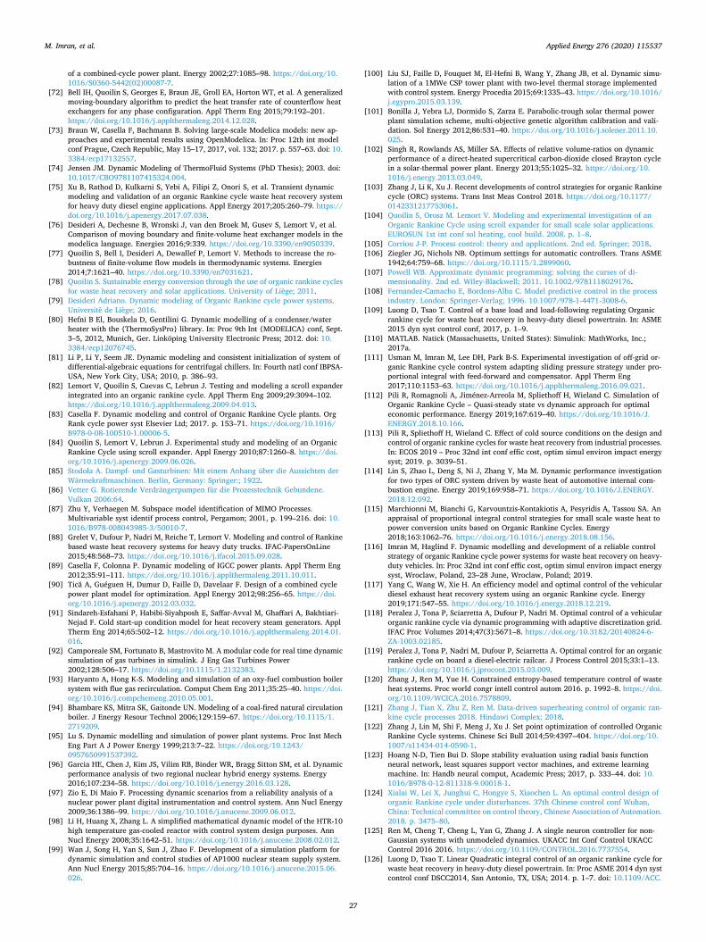
of a combined-cycle power plant. Energy 2002;27:1085–98. https://doi.org/10.1016/S0360-5442(02)00087-7.

[72] Bell IH, Quoilin S, Georges E, Braun JE, Groll EA, Horton WT, et al. A generalizedmoving-boundary algorithm to predict the heat transfer rate of counterflow heatexchangers for any phase configuration. Appl Therm Eng 2015;79:192–201.https://doi.org/10.1016/j.applthermaleng.2014.12.028.

[73] Braun W, Casella F, Bachmann B. Solving large-scale Modelica models: new ap-proaches and experimental results using OpenModelica. In: Proc 12th int modelconf Prague, Czech Republic, May 15–17, 2017, vol. 132; 2017. p. 557–63. doi: 10.3384/ecp17132557.

[74] Jensen JM. Dynamic Modeling of ThermoFluid Systems (PhD Thesis); 2003. doi:10.1017/CBO9781107415324.004.

[75] Xu B, Rathod D, Kulkarni S, Yebi A, Filipi Z, Onori S, et al. Transient dynamicmodeling and validation of an organic Rankine cycle waste heat recovery systemfor heavy duty diesel engine applications. Appl Energy 2017;205:260–79. https://doi.org/10.1016/j.apenergy.2017.07.038.

[76] Desideri A, Dechesne B, Wronski J, van den Broek M, Gusev S, Lemort V, et al.Comparison of moving boundary and finite-volume heat exchanger models in themodelica language. Energies 2016;9:339. https://doi.org/10.3390/en9050339.

[77] Quoilin S, Bell I, Desideri A, Dewallef P, Lemort V. Methods to increase the ro-bustness of finite-volume flow models in thermodynamic systems. Energies2014;7:1621–40. https://doi.org/10.3390/en7031621.

[78] Quoilin S. Sustainable energy conversion through the use of organic rankine cyclesfor waste heat recovery and solar applications. University of Liège; 2011.

[79] Desideri Adriano. Dynamic modeling of Organic Rankine cycle power systems.Universitè de Liège; 2016.

[80] Hefni B El, Bouskela D, Gentilini G. Dynamic modelling of a condenser/waterheater with the {ThermoSysPro} library. In: Proc 9th Int {MODELICA} conf, Sept.3–5, 2012, Munich, Ger. Linköping University Electronic Press; 2012. doi: 10.3384/ecp12076745.

[81] Li P, Li Y, Seem JE. Dynamic modeling and consistent initialization of system ofdifferential-algebraic equations for centrifugal chillers. In: Fourth natl conf IBPSA-USA, New York City, USA; 2010, p. 386–93.

[82] Lemort V, Quoilin S, Cuevas C, Lebrun J. Testing and modeling a scroll expanderintegrated into an organic rankine cycle. Appl Therm Eng 2009;29:3094–102.https://doi.org/10.1016/j.applthermaleng.2009.04.013.

[83] Casella F. Dynamic modeling and control of Organic Rankine Cycle plants. OrgRank cycle power syst Elsevier Ltd; 2017. p. 153–71. https://doi.org/10.1016/B978-0-08-100510-1.00006-5.

[84] Quoilin S, Lemort V, Lebrun J. Experimental study and modeling of an OrganicRankine Cycle using scroll expander. Appl Energy 2010;87:1260–8. https://doi.org/10.1016/j.apenergy.2009.06.026.

[85] Stodola A. Dampf- und Gasturbinen: Mit einem Anhang über die Aussichten derWärmekraftmaschinen. Berlin, Germany: Springer:; 1922.

[86] Vetter G. Rotierende Verdrängerpumpen für die Prozesstechnik Gebundene.Vulkan 2006:64.

[87] Zhu Y, Verhaegen M. Subspace model identification of MIMO Processes.Multivariable syst identif process control, Pergamon; 2001, p. 199–216. doi: 10.1016/B978-008043985-3/50010-7.

[88] Grelet V, Dufour P, Nadri M, Reiche T, Lemort V. Modeling and control of Rankinebased waste heat recovery systems for heavy duty trucks. IFAC-PapersOnLine2015;48:568–73. https://doi.org/10.1016/j.ifacol.2015.09.028.

[89] Casella F, Colonna P. Dynamic modeling of IGCC power plants. Appl Therm Eng2012;35:91–111. https://doi.org/10.1016/j.applthermaleng.2011.10.011.

[90] Tică A, Guéguen H, Dumur D, Faille D, Davelaar F. Design of a combined cyclepower plant model for optimization. Appl Energy 2012;98:256–65. https://doi.org/10.1016/j.apenergy.2012.03.032.

[91] Sindareh-Esfahani P, Habibi-Siyahposh E, Saffar-Avval M, Ghaffari A, Bakhtiari-Nejad F. Cold start-up condition model for heat recovery steam generators. ApplTherm Eng 2014;65:502–12. https://doi.org/10.1016/j.applthermaleng.2014.01.016.

[92] Camporeale SM, Fortunato B, Mastrovito M. A modular code for real time dynamicsimulation of gas turbines in simulink. J Eng Gas Turbines Power2002;128:506–17. https://doi.org/10.1115/1.2132383.

[93] Haryanto A, Hong K-S. Modeling and simulation of an oxy-fuel combustion boilersystem with flue gas recirculation. Comput Chem Eng 2011;35:25–40. https://doi.org/10.1016/j.compchemeng.2010.05.001.

[94] Bhambare KS, Mitra SK, Gaitonde UN. Modeling of a coal-fired natural circulationboiler. J Energy Resour Technol 2006;129:159–67. https://doi.org/10.1115/1.2719209.

[95] Lu S. Dynamic modelling and simulation of power plant systems. Proc Inst MechEng Part A J Power Energy 1999;213:7–22. https://doi.org/10.1243/0957650991537392.

[96] Garcia HE, Chen J, Kim JS, Vilim RB, Binder WR, Bragg Sitton SM, et al. Dynamicperformance analysis of two regional nuclear hybrid energy systems. Energy2016;107:234–58. https://doi.org/10.1016/j.energy.2016.03.128.

[97] Zio E, Di Maio F. Processing dynamic scenarios from a reliability analysis of anuclear power plant digital instrumentation and control system. Ann Nucl Energy2009;36:1386–99. https://doi.org/10.1016/j.anucene.2009.06.012.

[98] Li H, Huang X, Zhang L. A simplified mathematical dynamic model of the HTR-10high temperature gas-cooled reactor with control system design purposes. AnnNucl Energy 2008;35:1642–51. https://doi.org/10.1016/j.anucene.2008.02.012.

[99] Wan J, Song H, Yan S, Sun J, Zhao F. Development of a simulation platform fordynamic simulation and control studies of AP1000 nuclear steam supply system.Ann Nucl Energy 2015;85:704–16. https://doi.org/10.1016/j.anucene.2015.06.026.

[100] Liu SJ, Faille D, Fouquet M, El-Hefni B, Wang Y, Zhang JB, et al. Dynamic simu-lation of a 1MWe CSP tower plant with two-level thermal storage implementedwith control system. Energy Procedia 2015;69:1335–43. https://doi.org/10.1016/j.egypro.2015.03.139.

[101] Bonilla J, Yebra LJ, Dormido S, Zarza E. Parabolic-trough solar thermal powerplant simulation scheme, multi-objective genetic algorithm calibration and vali-dation. Sol Energy 2012;86:531–40. https://doi.org/10.1016/j.solener.2011.10.025.

[102] Singh R, Rowlands AS, Miller SA. Effects of relative volume-ratios on dynamicperformance of a direct-heated supercritical carbon-dioxide closed Brayton cyclein a solar-thermal power plant. Energy 2013;55:1025–32. https://doi.org/10.1016/j.energy.2013.03.049.

[103] Zhang J, Li K, Xu J. Recent developments of control strategies for organic Rankinecycle (ORC) systems. Trans Inst Meas Control 2018. https://doi.org/10.1177/0142331217753061.

[104] Quoilin S, Orosz M. Lemort V. Modeling and experimental investigation of anOrganic Rankine Cycle using scroll expander for small scale solar applications.EUROSUN 1st int conf sol heating, cool build. 2008. p. 1–8.

[105] Corriou J-P. Process control: theory and applications. 2nd ed. Springer; 2018.[106] Ziegler JG, Nichols NB. Optimum settings for automatic controllers. Trans ASME

1942;64:759–68. https://doi.org/10.1115/1.2899060.[107] Powell WB. Approximate dynamic programming: solving the curses of di-

mensionality. 2nd ed. Wiley-Blackwell; 2011. 10.1002/9781118029176.[108] Fernandez-Camacho E, Bordons-Alba C. Model predictive control in the process

industry. London: Springer-Verlag; 1996. 10.1007/978-1-4471-3008-6.[109] Luong D, Tsao T. Control of a base load and load-following regulating Organic

rankine cycle for waste heat recovery in heavy-duty diesel powertrain. In: ASME2015 dyn syst control conf, 2017, p. 1–9.

[110] MATLAB. Natick (Massachusetts, United States): Simulink: MathWorks, Inc.;2017a.

[111] Usman M, Imran M, Lee DH, Park B-S. Experimental investigation of off-grid or-ganic Rankine cycle control system adapting sliding pressure strategy under pro-portional integral with feed-forward and compensator. Appl Therm Eng2017;110:1153–63. https://doi.org/10.1016/j.applthermaleng.2016.09.021.

[112] Pili R, Romagnoli A, Jiménez-Arreola M, Spliethoff H, Wieland C. Simulation ofOrganic Rankine Cycle – Quasi-steady state vs dynamic approach for optimaleconomic performance. Energy 2019;167:619–40. https://doi.org/10.1016/J.ENERGY.2018.10.166.

[113] Pili R, Spliethoff H, Wieland C. Effect of cold source conditions on the design andcontrol of organic rankine cycles for waste heat recovery from industrial processes.In: ECOS 2019 – Proc 32nd int conf effic cost, optim simul environ impact energysyst; 2019. p. 3039–51.

[114] Lin S, Zhao L, Deng S, Ni J, Zhang Y, Ma M. Dynamic performance investigationfor two types of ORC system driven by waste heat of automotive internal com-bustion engine. Energy 2019;169:958–71. https://doi.org/10.1016/J.ENERGY.2018.12.092.

[115] Marchionni M, Bianchi G, Karvountzis-Kontakiotis A, Pesyridis A, Tassou SA. Anappraisal of proportional integral control strategies for small scale waste heat topower conversion units based on Organic Rankine Cycles. Energy2018;163:1062–76. https://doi.org/10.1016/j.energy.2018.08.156.

[116] Imran M, Haglind F. Dynamic modelling and development of a reliable controlstrategy of organic Rankine cycle power systems for waste heat recovery on heavy-duty vehicles. In: Proc 32nd int conf effic cost, optim simul environ impact energysyst, Wroclaw, Poland, 23–28 June, Wroclaw, Poland; 2019.

[117] Yang C, Wang W, Xie H. An efficiency model and optimal control of the vehiculardiesel exhaust heat recovery system using an organic Rankine cycle. Energy2019;171:547–55. https://doi.org/10.1016/j.energy.2018.12.219.

[118] Peralez J, Tona P, Sciarretta A, Dufour P, Nadri M. Optimal control of a vehicularorganic rankine cycle via dynamic programming with adaptive discretization grid.IFAC Proc Volumes 2014;47(3):5671–8. https://doi.org/10.3182/20140824-6-ZA-1003.02185.

[119] Peralez J, Tona P, Nadri M, Dufour P, Sciarretta A. Optimal control for an organicrankine cycle on board a diesel-electric railcar. J Process Control 2015;33:1–13.https://doi.org/10.1016/j.jprocont.2015.03.009.

[120] Zhang J, Ren M, Yue H. Constrained entropy-based temperature control of wasteheat systems. Proc world congr intell control autom 2016. p. 1992–8. https://doi.org/10.1109/WCICA.2016.7578809.

[121] Zhang J, Tian X, Zhu Z, Ren M. Data-driven superheating control of organic ran-kine cycle processes 2018. Hindawi Complex; 2018.

[122] Zhang J, Lin M, Shi F, Meng J, Xu J. Set point optimization of controlled OrganicRankine Cycle systems. Chinese Sci Bull 2014;59:4397–404. https://doi.org/10.1007/s11434-014-0590-1.

[123] Hoang N-D, Tien Bui D. Slope stability evaluation using radial basis functionneural network, least squares support vector machines, and extreme learningmachine. In: Handb neural comput, Academic Press; 2017, p. 333–44. doi: 10.1016/B978-0-12-811318-9.00018-1.

[124] Xialai W, Lei X, Junghui C, Hongye S, Xiaochen L. An optimal control design oforganic Rankine cycle under disturbances. 37th Chinese control conf Wuhan,China: Technical committee on control theory, Chinese Association of Automation.2018. p. 3475–80.

[125] Ren M, Cheng T, Cheng L, Yan G, Zhang J. A single neuron controller for non-Gaussian systems with unmodeled dynamics. UKACC Int Conf Control UKACCControl 2016 2016. https://doi.org/10.1109/CONTROL.2016.7737554.

[126] Luong D, Tsao T. Linear Quadratic integral control of an organic rankine cycle forwaste heat recovery in heavy-duty diesel powertrain. In: Proc ASME 2014 dyn systcontrol conf DSCC2014, San Antonio, TX, USA; 2014. p. 1–7. doi: 10.1109/ACC.


27

https://doi.org/10.1016/S0360-5442(02)00087-7

https://doi.org/10.1016/S0360-5442(02)00087-7


http://10.3384/ecp17132557

http://10.3384/ecp17132557

http://10.1017/CBO9781107415324.004



https://doi.org/10.3390/en9050339

https://doi.org/10.3390/en7031621





http://10.3384/ecp12076745

http://10.3384/ecp12076745


https://doi.org/10.1016/B978-0-08-100510-1.00006-5

https://doi.org/10.1016/B978-0-08-100510-1.00006-5







http://10.1016/B978-008043985-3/50010-7

http://10.1016/B978-008043985-3/50010-7







https://doi.org/10.1115/1.2132383

https://doi.org/10.1016/j.compchemeng.2010.05.001

https://doi.org/10.1016/j.compchemeng.2010.05.001

https://doi.org/10.1115/1.2719209

https://doi.org/10.1115/1.2719209

https://doi.org/10.1243/0957650991537392

https://doi.org/10.1243/0957650991537392


https://doi.org/10.1016/j.anucene.2009.06.012






https://doi.org/10.1016/j.solener.2011.10.025

https://doi.org/10.1016/j.solener.2011.10.025



https://doi.org/10.1177/0142331217753061

https://doi.org/10.1177/0142331217753061





https://doi.org/10.1115/1.2899060






https://doi.org/10.1016/J.ENERGY.2018.10.166






https://doi.org/10.3182/20140824-6-ZA-1003.02185

https://doi.org/10.3182/20140824-6-ZA-1003.02185

https://doi.org/10.1016/j.jprocont.2015.03.009

https://doi.org/10.1109/WCICA.2016.7578809

https://doi.org/10.1109/WCICA.2016.7578809



https://doi.org/10.1007/s11434-014-0590-1

https://doi.org/10.1007/s11434-014-0590-1

http://10.1016/B978-0-12-811318-9.00018-1

http://10.1016/B978-0-12-811318-9.00018-1





https://doi.org/10.1109/CONTROL.2016.7737554

http://10.1109/ACC.2014.6858907

2014.6858907.[127] Hernandez A, Ruiz F, Desideri A, Ionescu C, Quoilin S, Lemort V, et al. Nonlinear

identification and control of Organic Rankine Cycle systems using sparse poly-nomial models. 2016 IEEE Conf Control Appl CCA 2016 2016. p. 1012–7. https://doi.org/10.1109/CCA.2016.7587946.

[128] Hernandez A, Desideri A, Ionescu C, Quoilin S, Lemort V, De Keyser R. Increasingthe efficiency of Organic Rankine Cycle technology by means of multivariablepredictive control. IFAC Proc 2014;47:2195–200. https://doi.org/10.3182/20140824-6-ZA-1003.01796.

[129] Hernandez A, Desideri A, Ionescu C, Quoilin S, Lemort V, Keyser R De.Experimental study of Predictive Control strategies for optimal operation ofOrganic Rankine Cycle systems. In: 2015 Eur control conf, Linz, Austria; 2015, p.2259–64.

[130] Zhang J, Zhang T, Lin M, Hou G, Li K. Multiple model predictive control forOrganic Rankine Cycle (ORC) based waste heat energy conversion systems. In:2016 UKACC 11th int conf control, Belfast: 2016, p. 1–7.

[131] Pierobon L, Chan R, Li X, Iyengar K, Haglind F, Ydstie E. Model predictive controlof offshore power stations with waste heat recovery. J Eng Gas Turbines Power2016;138:71801.

[132] Rahmani MA, Alamir M, Gualino D, Rieu V. Nonlinear Dynamic ModelIdentification and MPC control of an Organic Rankine Cycle (ORC) based SolarThermal Power Plant. In: 2015 Eur control conf, Linz, Austria; 2015. p. 2544–51.

[133] Grelet V, Dufour P, Nadri M, Lemort V, Reiche T. Explicit multi-model predictivecontrol of a waste heat Rankine based system for heavy duty trucks. In: Proc IEEEconf decis control 2015. 54rd IEEE. p. 179–84. doi: 10.1109/CDC.2015.7402105.

[134] Petr P, Schröder C, Köhler J, Gräber M. Optimal control of waste heat recoverysystems applying nonlinear model predictive control (NMPC). In: 3RD int seminORC power syst. Oct. 12–14, 2015, Brussels, Belgium, Brussels, Belgium; 2015. p.1–10.

[135] Elmqvist Hilding. Modelica—A unified object-oriented language for physical sys-tems modeling. Simul Pract Theory 1997. https://doi.org/10.1016/s0928-4869(97)84257-7.

[136] Hernandez A, Desideri A, Gusev S, Ionescu CM, Den Broek M, Van Quoilin S, et al.Design and experimental validation of an adaptive control law to maximize thepower generation of a small-scale waste heat recovery system. Appl Energy2017;203:549–59. https://doi.org/10.1016/j.apenergy.2017.06.069.

[137] Wu X, Chen J, Xie L. Fast economic nonlinear model predictive control strategy ofOrganic Rankine Cycle for waste heat recovery: Simulation-based studies. Energy2019;180:520–34. https://doi.org/10.1016/J.ENERGY.2019.05.023.

[138] Koppauer H, Kemmetmüller W, Kugi A. Model predictive control of an automotivewaste heat recovery system. Control Eng Pract 2018;81:28–42. https://doi.org/10.

1016/J.CONENGPRAC.2018.09.005.[139] Rathod D, Xu B, Filipi Z, Hoffman M. An experimentally validated, energy focused,

optimal control strategy for an Organic Rankine Cycle waste heat recovery system.Appl Energy 2019;256:113991. https://doi.org/10.1016/J.APENERGY.2019.113991.

[140] Zhang J, Zhou Y, Li Y, Hou G, Fang F. Generalized predictive control applied inwaste heat recovery power plants. Appl Energy 2013;102:320–6. https://doi.org/10.1016/j.apenergy.2012.07.038.

[141] Zhang J, Feng J, Zhou Y, Fang F, Yue H. Linear active disturbance rejection controlof waste heat recovery systems with organic Rankine cycles. Energies2012;5:5111–25. https://doi.org/10.3390/en5125111.

[142] Yebi A, Xu B, Liu X, Shutty J, Anschel P, Filipi Z, et al. Estimation and predictivecontrol of a parallel evaporator diesel engine waste heat recovery system. IEEETrans Control Syst Technol 2019;27:282–95. https://doi.org/10.1109/TCST.2017.2759104.

[143] Hernandez A, Desideri A, Ionescu C, De Keyser R, Lemort V, Quoilin S. Real-timeoptimization of organic Rankine cycle systems by extremum-seeking control.Energies 2016;9:334. https://doi.org/10.3390/en9050334.

[144] Zhang J, Song G, Yannan C, Guolian H. Multivariable robust control for organicrankine cycle based waste heat. Recovery systems IEEE 8th conf ind electron appl.2013. p. 85–9.

[145] Wang R, Wang C, Zhao X, Zhang W. Neuro-PID control of heat exchanger in anOrganic Rankine Cycle system for waste heat recovery. 2011 Int Conf AdvMechatron Syst. 2011. p. 191–5.

[146] Torregrosa A, Galindo J, Dolz V, Royo-Pascual L, Haller R, Melis J. Dynamic testsand adaptive control of a bottoming organic Rankine cycle of IC engine usingswash-plate expander. Energy Convers Manag 2016;126:168–76. https://doi.org/10.1016/j.enconman.2016.07.078.

[147] Padula F, Sandrini R, Cominardi G. Adaptive PI control of an organic Rankinecycle power plant. IFAC Proc Vol 2012;45(3):459–64. https://doi.org/10.3182/20120328-3-IT-3014.00078.

[148] Imran M, Haglind F, Lemort V, Meroni A. Optimization of organic rankine cyclepower systems for waste heat recovery on heavy-duty vehicles considering theperformance, cost, mass and volume of the system. Energy 2019;180:229–41.https://doi.org/10.1016/J.ENERGY.2019.05.091.

[149] Zhang J, Lin M, Fang F, Xu J, Li K. Gain scheduling control of waste heat energyconversion systems based on an LPV (linear parameter varying) model. Energy2016;107:773–83. https://doi.org/10.1016/j.energy.2016.04.064.

[150] Grelet V, Dufour P, Nadri M, Lemort V, Reiche T. Explicit multi-model predictivecontrol of a waste heat Rankine based system for heavy duty trucks. Conf DecisControl (CDC) 2015;2:179–84.


28

http://10.1109/ACC.2014.6858907

https://doi.org/10.1109/CCA.2016.7587946

https://doi.org/10.1109/CCA.2016.7587946

https://doi.org/10.3182/20140824-6-ZA-1003.01796

https://doi.org/10.3182/20140824-6-ZA-1003.01796




http://10.1109/CDC.2015.7402105

https://doi.org/10.1016/s0928-4869(97)84257-7

https://doi.org/10.1016/s0928-4869(97)84257-7



https://doi.org/10.1016/J.CONENGPRAC.2018.09.005

https://doi.org/10.1016/J.CONENGPRAC.2018.09.005

https://doi.org/10.1016/J.APENERGY.2019.113991

https://doi.org/10.1016/J.APENERGY.2019.113991



https://doi.org/10.3390/en5125111

https://doi.org/10.1109/TCST.2017.2759104

https://doi.org/10.1109/TCST.2017.2759104

https://doi.org/10.3390/en9050334









https://doi.org/10.3182/20120328-3-IT-3014.00078

https://doi.org/10.3182/20120328-3-IT-3014.00078






Documents

Dynamic modeling and control strategies of organic Rankine