Embed Size (px)
Citation preview

Graduate Theses and Dissertations Iowa State University Capstones, Theses andDissertations
2010
Dynamic modeling and ascent flight control ofAres-I Crew Launch VehicleWei DuIowa State University
Follow this and additional works at: https://lib.dr.iastate.edu/etd
Part of the Aerospace Engineering Commons
This Dissertation is brought to you for free and open access by the Iowa State University Capstones, Theses and Dissertations at Iowa State UniversityDigital Repository. It has been accepted for inclusion in Graduate Theses and Dissertations by an authorized administrator of Iowa State UniversityDigital Repository. For more information, please contact [email protected].
Recommended CitationDu, Wei, "Dynamic modeling and ascent flight control of Ares-I Crew Launch Vehicle" (2010). Graduate Theses and Dissertations.11540.https://lib.dr.iastate.edu/etd/11540

Dynamic modeling and ascent flight control of Ares-I Crew Launch Vehicle
by
Wei Du
A dissertation submitted to the graduate faculty
in partial fulfillment of the requirements for the degree of
DOCTOR OF PHILOSOPHY
Major: Aerospace Engineering
Program of Study Committee:Bong Wie, Major Professor
Ping LuThomas J. Rudolphi
Zhijian WangJohn Basart
Iowa State University
Ames, Iowa
2010
Copyright c© Wei Du, 2010. All rights reserved.

ii
TABLE OF CONTENTS
LIST OF TABLES . . . . . . . . . . . . . . . . . . . . . . . . . . . . . . . . . . . vi
LIST OF FIGURES . . . . . . . . . . . . . . . . . . . . . . . . . . . . . . . . . . vii
ACKNOWLEDGEMENTS . . . . . . . . . . . . . . . . . . . . . . . . . . . . . . xiii
ABSTRACT . . . . . . . . . . . . . . . . . . . . . . . . . . . . . . . . . . . . . . . xiv
NOMENCLATURE . . . . . . . . . . . . . . . . . . . . . . . . . . . . . . . . . . xvi
CHAPTER 1. INTRODUCTION . . . . . . . . . . . . . . . . . . . . . . . . . 1
1.1 Overview . . . . . . . . . . . . . . . . . . . . . . . . . . . . . . . . . . . . . . . 1
1.2 Ares-I Configuration . . . . . . . . . . . . . . . . . . . . . . . . . . . . . . . . . 2
1.3 Ares-I Mission Profile . . . . . . . . . . . . . . . . . . . . . . . . . . . . . . . . 3
1.4 Interaction Between Structures and Flight Control System . . . . . . . . . . . . 5
1.5 Underactuated Control Problem . . . . . . . . . . . . . . . . . . . . . . . . . . 6
CHAPTER 2. 6-DEGREE-OF-FEEDOM DYNAMIC MODELING . . . . . 7
2.1 Introduction . . . . . . . . . . . . . . . . . . . . . . . . . . . . . . . . . . . . . . 7
2.2 Reference Frames and Rotational Kinematics . . . . . . . . . . . . . . . . . . . 8
2.2.1 Earth-Centered Inertial Reference Frame . . . . . . . . . . . . . . . . . 8
2.2.2 Earth-Fixed Equatorial Reference Frame . . . . . . . . . . . . . . . . . . 9
2.2.3 Body-Fixed Reference Frame . . . . . . . . . . . . . . . . . . . . . . . . 10
2.2.4 Structural Reference Frame . . . . . . . . . . . . . . . . . . . . . . . . . 10
2.2.5 Earth-Fixed Launch Pad Reference Frame . . . . . . . . . . . . . . . . . 11
2.2.6 Euler Angles and Quaternions . . . . . . . . . . . . . . . . . . . . . . . 11
2.2.7 Initial Position of Ares-I CLV on the Launch Pad . . . . . . . . . . . . . 13

iii
2.3 The 6-DOF Equations of Motion . . . . . . . . . . . . . . . . . . . . . . . . . . 14
2.3.1 Aerodynamic Forces and Moments . . . . . . . . . . . . . . . . . . . . . 15
2.3.2 Gravity Model . . . . . . . . . . . . . . . . . . . . . . . . . . . . . . . . 16
2.3.3 Rocket Propulsion Model . . . . . . . . . . . . . . . . . . . . . . . . . . 17
2.3.4 Guidance and Control . . . . . . . . . . . . . . . . . . . . . . . . . . . . 18
2.3.5 Flexible-Body Modes . . . . . . . . . . . . . . . . . . . . . . . . . . . . . 19
2.4 Simulation Results of the Rigid Body Ares-I Crew Launch Vehicle . . . . . . . 21
CHAPTER 3. ANALYSIS AND DESIGN OF ASCENT FLIGHT CON-
TROL SYSTEMS . . . . . . . . . . . . . . . . . . . . . . . . . . . . . . . . . 33
3.1 Introduction . . . . . . . . . . . . . . . . . . . . . . . . . . . . . . . . . . . . . . 33
3.2 Pitch Control Analysis of Rigid Launch Vehicles . . . . . . . . . . . . . . . . . 34
3.3 Pitch Control of a Rigid-Body Model of the Ares-I CLV . . . . . . . . . . . . . 39
3.4 Flexible-Body Control of an Ares-I Reference Model . . . . . . . . . . . . . . . 41
3.5 NMP Structural Filter Design . . . . . . . . . . . . . . . . . . . . . . . . . . . . 46
3.6 Robust Analysis for Structural Filters Design . . . . . . . . . . . . . . . . . . . 49
3.6.1 Uncertainty Description of Rigid-Body Model . . . . . . . . . . . . . . . 49
3.6.2 Uncertainty Description of Flexible-Body Model . . . . . . . . . . . . . 51
3.6.3 Robust Stability Analysis . . . . . . . . . . . . . . . . . . . . . . . . . . 54
CHAPTER 4. UNCONTROLLED ROLL DRIFT . . . . . . . . . . . . . . . . 58
4.1 Introduction . . . . . . . . . . . . . . . . . . . . . . . . . . . . . . . . . . . . . . 58
4.2 Pitch/Yaw Closed-Loop Instability Caused by Uncontrolled Roll Drift . . . . . 59
4.3 Stability Analysis . . . . . . . . . . . . . . . . . . . . . . . . . . . . . . . . . . . 61
4.3.1 Simplified Nonlinear Closed-Loop Pitch/Yaw Dynamics . . . . . . . . . 62
4.3.2 Linear Stability Analysis . . . . . . . . . . . . . . . . . . . . . . . . . . . 63
4.3.3 Nonlinear Stability Analysis . . . . . . . . . . . . . . . . . . . . . . . . . 68
4.4 New Pitch/Yaw Control Logic with Modified Commanded Quaternions . . . . 79
4.5 Simple Adjustment of Control Gains . . . . . . . . . . . . . . . . . . . . . . . . 85
4.5.1 Rigid Body 6-DOF Nonlinear Simulation Results . . . . . . . . . . . . . 86

iv
CHAPTER 5. UNDERACTUATED CONTROL PROBLEM OF AN AX-
ISYMMETRIC RIGID BODY . . . . . . . . . . . . . . . . . . . . . . . . . 89
5.1 Introduction . . . . . . . . . . . . . . . . . . . . . . . . . . . . . . . . . . . . . . 89
5.2 Steady-State Oscillations . . . . . . . . . . . . . . . . . . . . . . . . . . . . . . 91
5.3 Modified Attitude Quaternion Feedback Control Law . . . . . . . . . . . . . . . 98
5.4 Nonlinear Stability Analysis . . . . . . . . . . . . . . . . . . . . . . . . . . . . . 98
5.5 Simulation Results . . . . . . . . . . . . . . . . . . . . . . . . . . . . . . . . . . 99
5.6 A Special Case . . . . . . . . . . . . . . . . . . . . . . . . . . . . . . . . . . . . 108
CHAPTER 6. CONCLUSIONS . . . . . . . . . . . . . . . . . . . . . . . . . . 110
APPENDIX A. A SUMMARY OF THE 6-DOF EQUATIONS OF MOTION 112
APPENDIX B. ADDITIONAL FIGURES FROM 6-DOF SIMULATION . 114
B.1 Atmospheric Model . . . . . . . . . . . . . . . . . . . . . . . . . . . . . . . . . . 114
B.2 Aerodynamic Coefficient . . . . . . . . . . . . . . . . . . . . . . . . . . . . . . . 117
APPENDIX C. LINEARIZATION RESULTS . . . . . . . . . . . . . . . . . . 122
C.1 Nonlinear 6-DOF Equations . . . . . . . . . . . . . . . . . . . . . . . . . . . . . 122
C.2 Linear Rigid-Body Model . . . . . . . . . . . . . . . . . . . . . . . . . . . . . . 123
C.3 Linear State-Space Equations . . . . . . . . . . . . . . . . . . . . . . . . . . . . 125
C.4 Linear Flexible-Body Model . . . . . . . . . . . . . . . . . . . . . . . . . . . . . 127
APPENDIX D. ATTITUDE ERROR QUATERNION KINEMATIC DIF-
FERENTIAL EQUATIONS . . . . . . . . . . . . . . . . . . . . . . . . . . . 129
APPENDIX E. LINEAR MODEL OF UNCONTROLLED ROLL DRIFT
WITH AERODYNAMIC DISTURBANCE . . . . . . . . . . . . . . . . . . 131
APPENDIX F. DERIVATION OF A STEADY-STATE OSCILLATION . . 133
F.1 A Steady-State Oscillation of the Autonomous System . . . . . . . . . . . . . . 133
F.2 Solution of the Quadratic Matrix Equation . . . . . . . . . . . . . . . . . . . . 135
F.3 State Equations of the Steady-State Oscillation . . . . . . . . . . . . . . . . . . 137

v
APPENDIX G. DERIVATION OF THE DERIVATIVE OF A LYAPUNOV
FUNCTION CANDIDATE . . . . . . . . . . . . . . . . . . . . . . . . . . . . 140
BIBLIOGRAPHY . . . . . . . . . . . . . . . . . . . . . . . . . . . . . . . . . . . 142

vi
LIST OF TABLES
Table 2.1 Initial conditions at liftoff . . . . . . . . . . . . . . . . . . . . . . . . . 22
Table 3.1 Ares-I reference parameters at t = 60 sec . . . . . . . . . . . . . . . . . 39
Table 3.2 Ares-I structural bending modes for the pitch axis . . . . . . . . . . . . 41
Table 3.3 Ares-I structural bending modes for the yaw axis . . . . . . . . . . . . 41
Table 3.4 Ares-I rigid-body parametric uncertainty . . . . . . . . . . . . . . . . . 50
Table 4.1 Reference Ares-I CLV parameters at t = 60 sec. . . . . . . . . . . . . . 62
Table 4.2 Routh arrays. . . . . . . . . . . . . . . . . . . . . . . . . . . . . . . . . 64
Table 4.3 Three cases for root locus stability analysis. . . . . . . . . . . . . . . . 65
Table 4.4 Three simulation cases for nonlinear stability analysis. . . . . . . . . . 70
Table 5.1 Ares-I reference parameters at t = 60 sec . . . . . . . . . . . . . . . . . 92
Table 5.2 Parameters of steady-state oscillation M2 . . . . . . . . . . . . . . . . . 93
Table 5.3 Simulation cases with p = 0.005 rad/sec . . . . . . . . . . . . . . . . . 99

vii
LIST OF FIGURES
Figure 1.1 Comparison of Space Shuttle, Ares-I, Ares-V, and Saturn V launch
vehicles [1]. . . . . . . . . . . . . . . . . . . . . . . . . . . . . . . . . . 1
Figure 1.2 Ares-I CLV configuration [2]. . . . . . . . . . . . . . . . . . . . . . . . 2
Figure 1.3 Flexible mode shapes and sensor locations of the Ares-I Crew Launch
Vehicle [1]. Currently, rate-gyro blending is not considered for the Ares-I. 3
Figure 1.4 Ares-I CLV mission profile [2]. . . . . . . . . . . . . . . . . . . . . . . 4
Figure 1.5 Interaction between the ascent flight control and the structural bending
mode. . . . . . . . . . . . . . . . . . . . . . . . . . . . . . . . . . . . . 5
Figure 2.1 Ares-I CLV 6-DOF simulation block diagram. . . . . . . . . . . . . . . 7
Figure 2.2 Illustration of Earth-centered inertial reference frame ~I, ~J, ~K, Earth-
fixed reference frame ~Ie, ~Je, ~Ke, structural reference frame ~is,~js,~ks,
and body-fixed reference frame ~i,~j,~k. . . . . . . . . . . . . . . . . . 8
Figure 2.3 Launch Complex 39B at Kennedy Space Center . . . . . . . . . . . . . 9
Figure 2.4 Earth-fixed launch pad reference frame with a local tangent plan at
Launch Complex 39B at Kennedy Space Center. . . . . . . . . . . . . 11
Figure 2.5 Illustration of the Earth-centered inertial reference frame with ~I, ~J, ~K,
the Earth-fixed launch pad (up, east, north) reference frame, and the
Ares-I orientation with ~i,~j,~k on Launch Complex 39B. . . . . . . . . 13
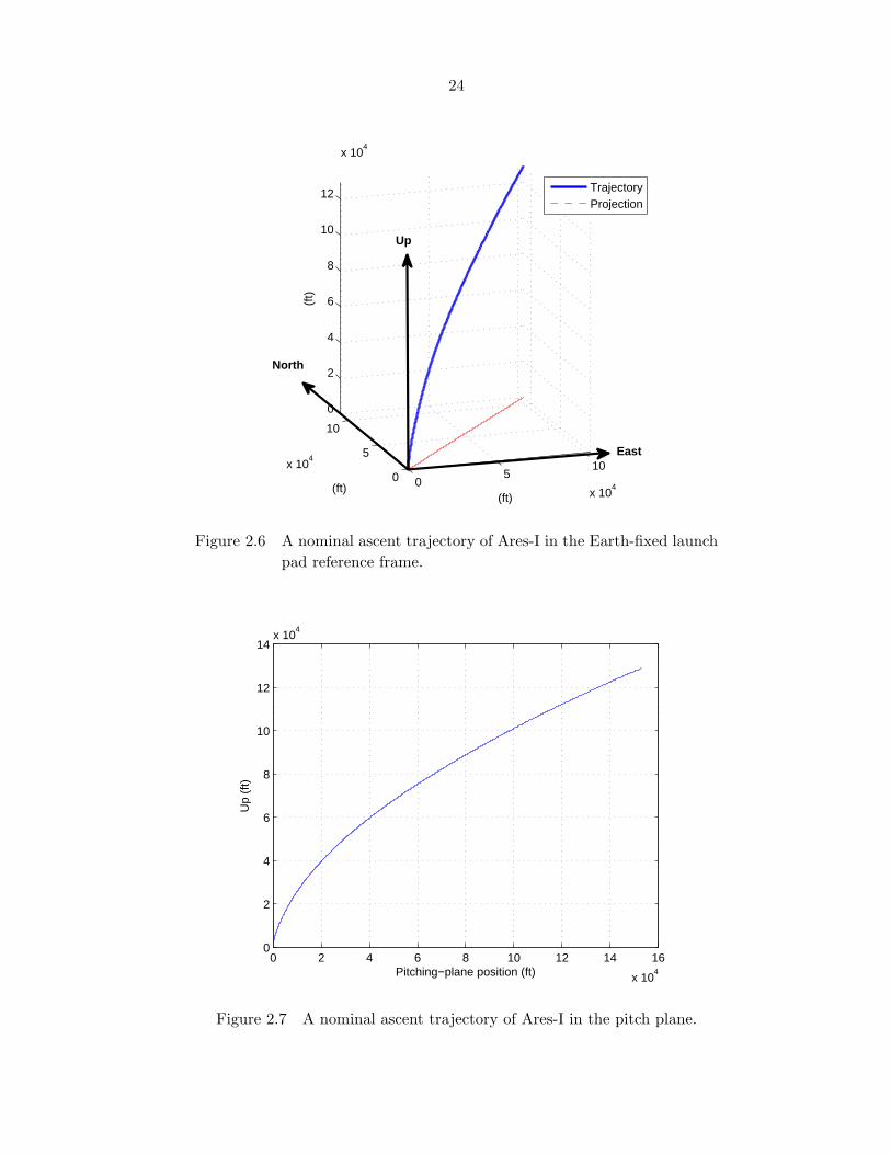
Figure 2.6 A nominal ascent trajectory of Ares-I in the Earth-fixed launch pad
reference frame. . . . . . . . . . . . . . . . . . . . . . . . . . . . . . . . 24
Figure 2.7 A nominal ascent trajectory of Ares-I in the pitch plane. . . . . . . . . 24

viii
Figure 2.8 Time histories of conventional roll, pitch, and yaw angles, (φ, θ, ψ), of
the Ares-I CLV. . . . . . . . . . . . . . . . . . . . . . . . . . . . . . . . 25
Figure 2.9 Trajectory in ECI. . . . . . . . . . . . . . . . . . . . . . . . . . . . . . 25
Figure 2.10 Center of pressure and center of gravity. . . . . . . . . . . . . . . . . . 26
Figure 2.11 Center of gravity offset. . . . . . . . . . . . . . . . . . . . . . . . . . . . 26
Figure 2.12 Relative velocity. . . . . . . . . . . . . . . . . . . . . . . . . . . . . . . 27
Figure 2.13 Altitude. . . . . . . . . . . . . . . . . . . . . . . . . . . . . . . . . . . . 27
Figure 2.14 Mach number. . . . . . . . . . . . . . . . . . . . . . . . . . . . . . . . . 28
Figure 2.15 Dynamic pressure. . . . . . . . . . . . . . . . . . . . . . . . . . . . . . 28
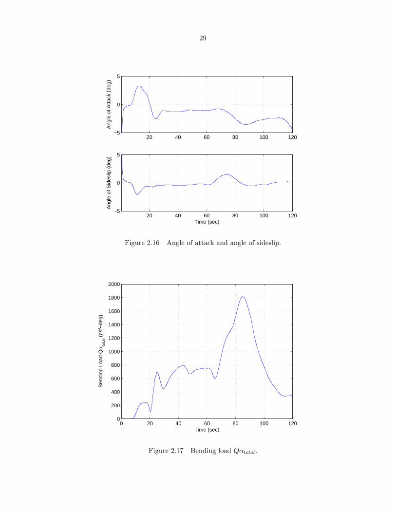
Figure 2.16 Angle of attack and angle of sideslip. . . . . . . . . . . . . . . . . . . . 29
Figure 2.17 Bending load Qαtotal. . . . . . . . . . . . . . . . . . . . . . . . . . . . . 29
Figure 2.18 RCS torque. . . . . . . . . . . . . . . . . . . . . . . . . . . . . . . . . . 30
Figure 2.19 Angular velocity. . . . . . . . . . . . . . . . . . . . . . . . . . . . . . . 30
Figure 2.20 Euler angles. . . . . . . . . . . . . . . . . . . . . . . . . . . . . . . . . . 31
Figure 2.21 Attitude quaternion. . . . . . . . . . . . . . . . . . . . . . . . . . . . . 31
Figure 2.22 Attitude-error quaternion. . . . . . . . . . . . . . . . . . . . . . . . . . 32
Figure 2.23 Gimbal angles. . . . . . . . . . . . . . . . . . . . . . . . . . . . . . . . . 32
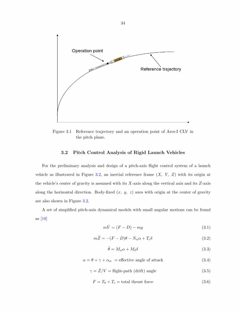
Figure 3.1 Reference trajectory and an operation point of Ares-I CLV in the pitch
plane. . . . . . . . . . . . . . . . . . . . . . . . . . . . . . . . . . . . . 34
Figure 3.2 A simplified dynamic model of a launch vehicle for preliminary pitch
control design. All angles are assumed to be small. . . . . . . . . . . . 35
Figure 3.3 Poles and zeros of Ares-I CLV rigid-body model transfer function. . . . 40
Figure 3.4 Root locus vs overall loop gain K of the pitch control system of a rigid
Ares-I model. . . . . . . . . . . . . . . . . . . . . . . . . . . . . . . . . 40
Figure 3.5 Block diagram of attitude control loop with flexible-body dynamics. . . 42
Figure 3.6 Flexible structure in the pitch plane. . . . . . . . . . . . . . . . . . . . 43
Figure 3.7 Block diagram of the flexible-body part of the pitch transfer function. 44
Figure 3.8 Pitch transfer function model of a reference model of the Ares-I CLV. . 44

ix
Figure 3.9 Root locus of the pitch control system without structural filters. . . . . 45
Figure 3.10 Root locus of the pitch control system with two NMP structural filters. 47
Figure 3.11 Impulse responses for the pitch attitude θ (in degrees) of the flexible
Ares-I. . . . . . . . . . . . . . . . . . . . . . . . . . . . . . . . . . . . . 47
Figure 3.12 Impulse responses for the pitch gimbal angle δ (in degrees) of the flexible
Ares-I. . . . . . . . . . . . . . . . . . . . . . . . . . . . . . . . . . . . . 48
Figure 3.13 General control configuration. . . . . . . . . . . . . . . . . . . . . . . . 50
Figure 3.14 M-∆ structure for robust stability analysis. . . . . . . . . . . . . . . . 51
Figure 3.15 Plant with multiplcative uncertainty. . . . . . . . . . . . . . . . . . . . 51
Figure 3.16 Bode plot of parameter uncertainty plant and perturbed plant samples. 52
Figure 3.17 Bode plot magnitude. . . . . . . . . . . . . . . . . . . . . . . . . . . . . 53
Figure 3.18 Block diagram of perturbed transfer function Gpi(s). . . . . . . . . . . 54
Figure 3.19 Bode plot samples of Gflex(s) with frequencies uncertainty and the
boundary of perturbed models∑3
i=1Gpi(s). . . . . . . . . . . . . . . . 55
Figure 3.20 Block diagram of perturbed attitude control system. . . . . . . . . . . 56
Figure 3.21 µ-plot for RS of structural filters design. . . . . . . . . . . . . . . . . . 57
Figure 4.1 Attitude quaternion for an unstable closed-loop system caused by un-
controlled roll drift. . . . . . . . . . . . . . . . . . . . . . . . . . . . . . 59
Figure 4.2 Euler angles for an unstable closed-loop system caused by uncontrolled
roll drift. . . . . . . . . . . . . . . . . . . . . . . . . . . . . . . . . . . . 60
Figure 4.3 Gimbal angles for an unstable closed-loop system caused by uncon-
trolled roll drift. . . . . . . . . . . . . . . . . . . . . . . . . . . . . . . . 60
Figure 4.4 A simplified block diagram representation of the quaternion based as-
cent flight control system of Ares-I CLV. . . . . . . . . . . . . . . . . . 62
Figure 4.5 Plot of the function B = 1−q24e
q4e. . . . . . . . . . . . . . . . . . . . . . . 65
Figure 4.6 Root locus plot for Case 1. . . . . . . . . . . . . . . . . . . . . . . . . . 66
Figure 4.7 Root locus plot for Case 2. . . . . . . . . . . . . . . . . . . . . . . . . . 67

x
Figure 4.8 Root locus plot for Case 3, showing closed-loop instability with a nom-
inal loop gain. . . . . . . . . . . . . . . . . . . . . . . . . . . . . . . . . 67
Figure 4.9 Trajectory on the spherical surface q21 + q24 + z2 = 1. . . . . . . . . . . 70
Figure 4.10 The positive invariant set M . . . . . . . . . . . . . . . . . . . . . . . . 71
Figure 4.11 The stable and unstable regions in M . . . . . . . . . . . . . . . . . . . 71
Figure 4.12 Angular velocity for Case 1. . . . . . . . . . . . . . . . . . . . . . . . . 72
Figure 4.13 Attitude quaternion for Case 1. . . . . . . . . . . . . . . . . . . . . . . 72
Figure 4.14 Phase portrait of q2 and q3 for Case 1. . . . . . . . . . . . . . . . . . . 73
Figure 4.15 Control inputs for Case 1. . . . . . . . . . . . . . . . . . . . . . . . . . 73
Figure 4.16 Angular velocity for Case 2. . . . . . . . . . . . . . . . . . . . . . . . . 74
Figure 4.17 Attitude quaternion for Case 2. . . . . . . . . . . . . . . . . . . . . . . 74
Figure 4.18 Phase portrait of q2 and q3 for Case 2. . . . . . . . . . . . . . . . . . . 75
Figure 4.19 Control inputs for Case 2. . . . . . . . . . . . . . . . . . . . . . . . . . 75
Figure 4.20 Angular velocity for Case 3. . . . . . . . . . . . . . . . . . . . . . . . . 76
Figure 4.21 Attitude quaternion for Case 3. . . . . . . . . . . . . . . . . . . . . . . 76
Figure 4.22 Phase portrait of q2 and q3 for Case 3. . . . . . . . . . . . . . . . . . . 77
Figure 4.23 q1-q2-q3 plot for Case 3. . . . . . . . . . . . . . . . . . . . . . . . . . . 77
Figure 4.24 Control inputs for Case 3. . . . . . . . . . . . . . . . . . . . . . . . . . 78
Figure 4.25 q2-q3 plot, from left to right q1 = 0,q1 = 0.2,q1 = 0.4,q1 = 0.6. . . . . . 78
Figure 4.26 A block diagram representation of a proposed method for computing a
new set of commanded attitude quaternion. . . . . . . . . . . . . . . . 79
Figure 4.27 Comparison of new and original attitude Euler angles command. . . . 81
Figure 4.28 Comparison of new and original attitude quaternion command. . . . . 82
Figure 4.29 Quaternion for a closed-loop system stabilized by the proposed control
logic employing modified commanded quaternion. . . . . . . . . . . . . 83
Figure 4.30 Euler angles for a closed-loop system stabilized by the proposed control
logic employing modified commanded quaternion. . . . . . . . . . . . . 83

xi
Figure 4.31 Gimbal angles for a closed-loop system stabilized by the proposed con-
trol logic employing modified commanded quaternion. . . . . . . . . . 84
Figure 4.32 Comparison of ascent trajectories: with roll control system vs. without
roll control system. . . . . . . . . . . . . . . . . . . . . . . . . . . . . . 84
Figure 4.33 Root locus plot for Case 3 but with a new derivative gain with γ = 4
in the pitch channel. . . . . . . . . . . . . . . . . . . . . . . . . . . . . 86
Figure 4.34 Attitude quaternion of 6-DOF nonlinear simulation with Kd = 4Kd. . . 87
Figure 4.35 Euler angles of 6-DOF nonlinear simulation with Kd = 4Kd. . . . . . . 87
Figure 4.36 Gimbal angles of 6-DOF nonlinear simulation with Kd = 4Kd. . . . . . 88
Figure 4.37 Comparison of ascent trajectories. . . . . . . . . . . . . . . . . . . . . . 88
Figure 5.1 Steady-state oscillations M1 and M2 on the spherical surface q21 + q24 +
z2 = 1. . . . . . . . . . . . . . . . . . . . . . . . . . . . . . . . . . . . . 93
Figure 5.2 Steady-state oscillations M1 and M2 on the surface of cone z =√q22 + q23. 94
Figure 5.3 Angular velocity of steady-state oscillation M2. . . . . . . . . . . . . . 94
Figure 5.4 Attitude quaternion of steady-state oscillation M2. . . . . . . . . . . . 95
Figure 5.5 Euler angles of steady-state oscillation M2. . . . . . . . . . . . . . . . . 95
Figure 5.6 Phase portrait of q and r of steady-state oscillation M2. . . . . . . . . 96
Figure 5.7 Phase portrait of q2 and q3 of steady-state oscillation M2. . . . . . . . 96
Figure 5.8 The relation between vectors (q, r)T and (q2, q3)T of steady-state os-
cillation M2. . . . . . . . . . . . . . . . . . . . . . . . . . . . . . . . . . 97
Figure 5.9 Gimbal angles of steady-state oscillation M2. . . . . . . . . . . . . . . . 97
Figure 5.10 Trajectory on the spherical surface q21 + q24 + z2 = 1 for Case 1. . . . . 100
Figure 5.11 Detailed trajectory on the spherical surface q21 + q24 + z2 = 1 for Case 1. 100
Figure 5.12 Angular velocity components q and r for Case 1. . . . . . . . . . . . . 101
Figure 5.13 Quaternion q1, q2 and q3 for Case 1. . . . . . . . . . . . . . . . . . . . 101
Figure 5.14 Euler angles for Case 1. . . . . . . . . . . . . . . . . . . . . . . . . . . 102
Figure 5.15 Gimbal angles for Case 1. . . . . . . . . . . . . . . . . . . . . . . . . . 102
Figure 5.16 Phase portrait of q and r for Case 1. . . . . . . . . . . . . . . . . . . . 103

xii
Figure 5.17 Phase portrait of q2 and q3 for Case 1. . . . . . . . . . . . . . . . . . . 103
Figure 5.18 Phase portrait of q1 and q4 for Case 1. . . . . . . . . . . . . . . . . . . 104
Figure 5.19 Trajectory on the spherical surface q21 + q24 + z2 = 1 for Case 2. . . . . 104
Figure 5.20 Detailed trajectory on the spherical surface q21 + q24 + z2 = 1 for Case 2. 105
Figure 5.21 Angular velocity components q and r for Case 2. . . . . . . . . . . . . 105
Figure 5.22 Quaternion q1, q2 and q3 for Case 2. . . . . . . . . . . . . . . . . . . . 106
Figure 5.23 Euler angles for Case 2. . . . . . . . . . . . . . . . . . . . . . . . . . . 106
Figure 5.24 Gimbal angles for Case 2. . . . . . . . . . . . . . . . . . . . . . . . . . 107
Figure B.1 Speed of sound . . . . . . . . . . . . . . . . . . . . . . . . . . . . . . . 114
Figure B.2 Density of air . . . . . . . . . . . . . . . . . . . . . . . . . . . . . . . . 115
Figure B.3 Wind profile . . . . . . . . . . . . . . . . . . . . . . . . . . . . . . . . . 115
Figure B.4 Base force . . . . . . . . . . . . . . . . . . . . . . . . . . . . . . . . . . 116
Figure B.5 CA . . . . . . . . . . . . . . . . . . . . . . . . . . . . . . . . . . . . . . 117
Figure B.6 CY β . . . . . . . . . . . . . . . . . . . . . . . . . . . . . . . . . . . . . 118
Figure B.7 CNα . . . . . . . . . . . . . . . . . . . . . . . . . . . . . . . . . . . . . 118
Figure B.8 CMpα . . . . . . . . . . . . . . . . . . . . . . . . . . . . . . . . . . . . . 119
Figure B.9 CMyβ . . . . . . . . . . . . . . . . . . . . . . . . . . . . . . . . . . . . . 119
Figure B.10 Rocket weight. . . . . . . . . . . . . . . . . . . . . . . . . . . . . . . . . 120
Figure B.11 Rocket thrust. . . . . . . . . . . . . . . . . . . . . . . . . . . . . . . . . 121
Figure B.12 Moments of inertia. . . . . . . . . . . . . . . . . . . . . . . . . . . . . . 121

xiii
ACKNOWLEDGEMENTS
I would first like to thank my supervisor, Dr. Bong Wie, for all his inspiration, guidance
and financial support throughout my study at Iowa State University. Dr. Wie provided me
a chance to make my dream, studying flight control system of a launch vehicle, come true. I
was influenced by his research philosophy, which placed great emphasis on the fundamental
knowledge and deep understanding of control theory. His words “there is no magic” and “what
is the next logical question” motivated me to finish my Ph.D. program step by step.
Meeting Dr. Ping Lu was another great fortune for me. His organized course on opti-
mal control and aerospace vehicle guidance reshaped my knowledge in those fields. Through
discussions with him, his intuition and sense of potential research direction opened my mind.
My appreciation also goes to all my committee members Dr. Thomas Rudolphi, Dr. Zhijian
Wang and Dr. John Basart for their valuable help and suggestions to my research. I would also
like to thank Dr. Nicola Elia who is a faculty in the Department of Electrical and Computer
Engineering. His big picture teaching style and enthusiasm in theoretical research made tedious
theorems visible and colorful.
I am indebted to my colleagues at ISU, including Anand Gopa Kumar, Insu Chang, Morgan
Baldwin, Matthew Hawkins, Zhongyuan Qian, Ying Zhou, De Huang, Haiyang Gao and a lot of
people in the Department of Aerospace Engineering. And I am especially grateful to Matthew
Hawkins for his help on polishing my writing.
My sincere thanks go to my parents for their advice and guidance throughout all my
education. And I am also thankful to my parents-in-law for their spiritual support.
Lastly, I wish to thank my wife Zhimei for all her love, support and sacrifice. She has
always stood beside me and encouraged me. To her I dedicate this dissertation.

xiv
ABSTRACT
This research focuses on dynamic modeling and ascent flight control of large flexible launch
vehicles such as the Ares-I Crew Launch Vehicle (CLV). A complete set of six-degrees-of-
freedom dynamic models of the Ares-I, incorporating its propulsion, aerodynamics, guidance
and control, and structural flexibility, is developed. NASA’s Ares-I reference model and the
SAVANT Simulink-based program are utilized to develop a Matlab-based simulation and lin-
earization tool for an independent validation of the performance and stability of the ascent
flight control system of large flexible launch vehicles. A linearized state-space model as well
as a non-minimum-phase transfer function model (which is typical for flexible vehicles with
non-collocated actuators and sensors) are validated for ascent flight control design and analysis.
This research also investigates fundamental principles of flight control analysis and design
for launch vehicles, in particular the classical “drift-minimum” and “load-minimum” control
principles. It is shown that an additional feedback of angle-of-attack can significantly improve
overall performance and stability, especially in the presence of unexpected large wind distur-
bances. For a typical “non-collocated actuator and sensor” control problem for large flexible
launch vehicles, non-minimum-phase filtering of “unstably interacting” bending modes is also
shown to be effective. The uncertainty model of a flexible launch vehicle is derived. The
robust stability of an ascent flight control system design, which directly controls the inertial
attitude-error quaternion and also employs the non-minimum-phase filters, is verified by the
framework of structured singular value (µ) analysis. Furthermore, nonlinear coupled dynamic
simulation results are presented for a reference model of the Ares-I CLV as another validation
of the feasibility of the ascent flight control system design.
Another important issue for a single main engine launch vehicle is stability under mal-

xv
function of the roll control system. The roll motion of the Ares-I Crew Launch Vehicle under
nominal flight conditions is actively stabilized by its roll control system employing thrusters.
This dissertation describes the ascent flight control design problem of Ares-I in the event of
disabled or failed roll control. A simple pitch/yaw control logic is developed for such a techni-
cally challenging problem by exploiting the inherent versatility of a quaternion-based attitude
control system. The proposed scheme requires only the desired inertial attitude quaternion
to be re-computed using the actual uncontrolled roll angle information to achieve an ascent
flight trajectory identical to the nominal flight case with active roll control. Another approach
that utilizes a simple adjustment of the proportional-derivative gains of the quaternion-based
flight control system without active roll control is also presented. This approach doesn’t re-
quire the re-computation of desired inertial attitude quaternion. A linear stability criterion
is developed for proper adjustments of attitude and rate gains. The linear stability analysis
results are validated by nonlinear simulations of the ascent flight phase. However, the first
approach, requiring a simple modification of the desired attitude quaternion, is recommended
for the Ares-I as well as other launch vehicles in the event of no active roll control.
Finally, the method derived to stabilize a large flexible launch vehicle in the event of
uncontrolled roll drift is generalized as a modified attitude quaternion feedback law. It is used
to stabilize an axisymmetric rigid body by two independent control torques.

xvi
NOMENCLATURE
a speed of sound = 1117 ft/s at sea level in the standard atmosphere
Ae nozzle exit area = 122.137 ft2
b reference body length = 12.16 ft
(cx, cy, cz) components of the center of mass location in the structural
reference frame with its origin at the top of vehicle
= (−220.31, 0.02, 0.01) ft at t = 0
CA axial force coefficient
CY β side force curve slope with respect to β
CN0 normal force coefficient at zero angle of attack
CNα normal force curve slope with respect to α
CMrβ rolling moment curve slope
CMp0 pitching moment coefficient at zero angle of attack
CMpα pitching moment curve slope
CMyβ yawing moment curve slope
CB/I direction cosine matrix of the frame B with respect to the frame I
C lateral (side) force
D drag (axial) force
Fbase base force
(Faero.xb, Faero.yb, Faero.zb) body-axis components of aerodynamic force
(Frkt.xb, Frkt.yb, Frkt.zb) body-axis components of solid rocket booster force
(Frcs.xb, Frcs.yb, Frcs.zb) body-axis components of RCS force
(Ftotal.xb, Ftotal.yb, Ftotal.zb) body-axis components of total force

xvii
(Ftotal.xi, Ftotal.yi, Ftotal.zi) inertial components of total force
(gx, gy, gz) inertial components of the gravitational acceleration
(~i,~j,~k) basis vectors of the body-fixed reference frame B
(~is,~js,~ks) basis vectors of the structural reference frame S
(~I, ~J, ~K) basis vectors of the Earth-centered inertial reference frame I
(~Ie, ~Je, ~Ke) basis vectors of the Earth-fixed equatorial rotating reference frame E
J2 Earth’s second-order zonal coefficient = 1.082631× 10⁻³
J3 Earth’s third-order zonal coefficient = −2.55× 10⁻⁶
J4 Earth’s fourth-order zonal coefficient = −1.61× 10⁻⁶
Kp proportional gain
Kd derivative gain
m vehicle’s mass
M Mach number
N normal force
p0 local atmospheric pressure
pe nozzle exit pressure
(p, q, r) body-axis components of ~ω
(q1, q2, q3, q4) attitude quaternion of the vehicle with respect to an inertial
reference frame
(q1c, q2c, q3c, q4c) desired attitude quaternion command from ascent guidance system
(q1e, q2e, q3e, q4e) attitude-error quaternion
(q1c, q2c, q3c, q4c) a modified set of desired attitude quaternion associated
with (θ1, θ2c, θ3c)
Q dynamic pressure
Re Earth’s equatorial radius = 20,925,646 ft
Rp Earth’s polar radius = 20,855,486 ft
~r vehicle’s position vector
r magnitude of ~r

xviii
S reference area = 116.2 ft2
T total thrust
T0 total vacuum thrust
T∞ thrust at any lower level in the atomosphere
(Taero.xb, Taero.yb, Taero.zb) body-axis components of aerodynamic torque
(Trkt.xb, Trkt.yb, Trkt.zb) body-axis components of solid rocket torque
(Trcs.xb, Trcs.yb, Trcs.zb) body-axis components of RCS torque
U Earth’s gravitational potential
(u, v, w) body-axis components of ~V
~V vehicle’s inertial velocity vector
Ve exit velocity of the solid rocket booster
~Vrel vehicle’s velocity vector relative to the Earth-fixed reference frame
~Vw velocity vector of the wind
~Vm air stream velocity vector
Vm magnitude of the air stream velocity
(Vm.xb, Vm.yb, Vm.zb) body-axis components of vehicle’s air stream velocity vector
(x, y, z) inertial components of vehicle’s position vector ~r
Xa aerodynamic reference point location in the structural frame = −275.6 ft
Xg gimbal attach point location in the structural frame = −296 ft
α angle of attack
β angle of sideslip
δy pitch gimbal angle (rotation about the body y-axis)
δz yaw gimbal angle (rotation about the body z-axis)
µ Earth’s gravitational parameter = 1.407644176× 1016 ft3/s2
φ Earth’s geocentric latitude
(θ1, θ2, θ3) Euler angles associated with (q1, q2, q3, q4) for
C1(θ1)← C2(θ2)← C3(θ3)
(θ1c, θ2c, θ3c) Euler angles associated with (q1c, q2c, q3c, q4c)

xix
(θ1, θ2c, θ3c) a modified set of Euler angles
ρ density of the air
η flexible-mode state vector
ζ damping ratio of the flexible modes = 0.005
Ω = diag(ωi) undamped natural frequency matrix of the flexible modes
~ω angular velocity vector of the vehicle
~ωe = ωe~K angular velocity vector of the Earth where ωe = 7.29× 10⁻⁵ rad/s

1
CHAPTER 1. INTRODUCTION
1.1 Overview
Figure 1.1 Comparison of Space Shuttle, Ares-I, Ares-V, and Saturn Vlaunch vehicles [1].
The Ares-I Crew Launch Vehicle (CLV), being developed by the National Aeronautics and
Space Administration (NASA) [1], is a large, slender, and aerodynamically unstable vehicle.
It will be used to launch astronauts to Low Earth Orbit and rendezvous with the International
Space Station (ISS) or NASA Exploration System Mission Directorate’s earth departure stage
for lunar or other future missions beyond Low Earth Orbit. In Figure 1.1, its overall con-
figuration is compared to other launch vehicles, including the Ares-V Cargo Launch Vehicle
and Saturn V. The Ares-I CLV is a two-stage rocket with a solid-propellant first stage derived
from the Shuttle Reusable Solid Rocket Motor/Booster and an upper stage employing a J-2X

2
engine derived from the Saturn J-2 engines.
1.2 Ares-I Configuration
Figure 1.2 Ares-I CLV configuration [2].
Ares-I CLV has an “in-line” configuration as illustrated in Figure 1.2, as opposed to the
Shuttle, which has the orbiter and crew placed beside the External Tank. In the event of an
emergency, the Orion Crew Module can be blasted away from the launch vehicle using the
Launch Abort System (LAS), which will fly directly upward, out of the way of the launch
vehicle.
The first stage is a new 5-segment solid rocket booster (SRB), derived from a 4-segment
space shuttle reusable solid rocket motor (RSRM). It will also include separation and recovery
systems, and SRB nozzle gimbal capability for thrust vector control (TVC). The second stage
or upper stage is powered by a liquid oxygen/liquid hydrogen constant-thrust J-2X engine. It
also contains avionics and other subsystems. The upper stage and first stage are connected by
the interstage, which also contains roll control system (RCS) [3] to prevent the vehicle from
spinning as it accelerates upward from the thrust of the SRB.
In addition to the LAS, upper stage, and first stage, the stack includes a forward skirt

3
and instrument unit, which connects the Orion to the Ares-I and contains the flight computer
for controlling the launch vehicle. The Ares-I navigation hardware will be located within an
instrumentation ring near the top of the second stage and just behind crew exploration vehicle
(CEV). An Inertial Measurement Unit (IMU) located in the instrument unit (at the top of
upper stage) will provide inertial position and velocity information to the navigation system
[4], and attitude quaternion and angular velocity to the Flight Control System (FCS). Pitch
and yaw body rates are obtained from two Rate Gyro Assemblies (RGAs) located near the
interstage and the first stage aft skirt (Figure 1.3).
Figure 1.3 Flexible mode shapes and sensor locations of the Ares-I CrewLaunch Vehicle [1]. Currently, rate-gyro blending is not consid-ered for the Ares-I.
1.3 Ares-I Mission Profile
As seen in Figure 1.4, ascent flight trajectory begins at lift-off and lasts until first stage
separation. It takes approximately 120 seconds. This dissertation will focus on flight simulation
and ascent flight control system analysis and design during the ascent flight phase. During this
phase, Ares-I will experience velocities up to Mach 4.5 at an altitude of about 130, 000 feet,

4
Figure 1.4 Ares-I CLV mission profile [2].
and a maximum dynamic pressure (Max Q) of approximately 800 pounds per square foot.
The ascent flight trajectory can be separated into three phases: vertical flight, transition
turn and gravity turn. After SRB ignition, the launch vehicle flies vertically until it has
cleared the launch tower. The vertical, stationary attitude flight of the launch vehicle lasts
approximately 6 seconds, and then it commences a combined pitch/roll maneuver in order
to head the crew window to the launch azimuth, which is defined as the angle between the
vertical ascent trajectory plane (or the so-called pitch plane) and a vector pointing from the
launch pad toward the North Pole. As a result, the required heads-down orientation of the
crew can be maintained during the ascent flight phase [5]. This maneuver is also known as the
transition turn [6]. The vehicle transitions from vertical rise to the gravity turn condition. It
will fly a gravity turn trajectory until burn out of the SRB and separation [7]. The gravity turn
maneuver is used to achieve an ascent trajectory with zero angle of attack and zero sideslip
angle (e.g. flying into the relative wind) by minimizing structural bending loads.
Since a detailed discussion of the launch vehicle guidance and trajectory optimization of
Ares-I CLV is beyond the scope of this dissertation, the reader is referred to the literature for

5
a more complete treatment [7, 8, 9].
1.4 Interaction Between Structures and Flight Control System
Figure 1.5 Interaction between the ascent flight control and the structuralbending mode.
A launch vehicle is essentially a long slender beam,thus it is structurally very flexible. IMUs
are placed along the vehicle body to sense angular displacement or rate for feedback control.
The IMU measures local elastic distortions as well as rigid body motion. As a result, one
significant risk for a large flexible launch vehicle ascent flight control system is the potential
for interaction between the ascent flight control and the structural bending mode. Because the
first bending mode frequency is usually close to the crossover regime of the rigid body control
system, the control system has the potential to excite the bending mode and destabilize the
vehicle dynamics [11].
This structural feedback problem can be illustrated by Figure 1.5. TVC actuators and

6
attitude sensors of launch vehicles are not collocated. The sensors pick up both rigid-body
motion of the vehicle and motion caused by structural deformations at the location of the
sensors. These deformations affect the command to the actuator (usually gimbaled rocket
engines). Since engines apply forces to the launch vehicle’s structure, energy can be fed into
the structure at various frequencies. This will reinforce elastic oscillations, leading ultimately
to structural failure of the vehicle.
Conventional roll-off filters and/or notch filters were often used in practice for the stabiliza-
tion of such unstably interacting bending modes of large flexible launch vehicles [10, 12, 13, 14,
15]. However, in [16, 20, 21], use of non-minimum-phase (NMP) structural filters was shown
to be very effective and robust in controlling flexible structures with non-collocated actuators
and sensors. In Chapter 3 it will be shown that the NMP filters can stabilize, effectively and
robustly, the bending modes of the Ares-I CLV.
1.5 Underactuated Control Problem
The active RCS of Ares-I CLV provides rotational azimuth control to perform a roll orien-
tation maneuver after lift-off and to mitigate against adverse roll torques [22]. It was harvested
from the Peacekeeper missile’s fourth stage axial thruster system. The challenge for the roll
control system is to be able to control large rolling moments, with continuously decreasing
principal moment of inertia during flight. RCS failure is a potential threat to the safety of
astronauts and launch vehicles. In Chapter 4, the problem of ascent flight control in the event
of uncontrolled roll drift will be discussed. Furthermore, it could be generalized as a typical
underactuated control problem [23, 24, 25, 26, 27]. In Chapter 5, methods developed to stabi-
lize Ares-I will be generalized as a method to stabilize an axisymmetric rigid body using two
control inputs.

7
CHAPTER 2. 6-DEGREE-OF-FEEDOM DYNAMIC MODELING
2.1 Introduction
A complete set of coupled dynamic models of the Ares-I CLV, incorporating its propulsion,
aerodynamics, guidance and control, and structural flexibility will be described in this chapter.
The Ares-I CLV is a large, slender, and aerodynamically unstable vehicle. NASA’s reference
model and SAVANT Simulink-based program [11, 28, 29], as well as various dynamic models
of launch vehicles developed previously in the literature [10, 16, 30, 31, 32], were utilized to
develop a Matlab-based simulation and linearization tool for an independent validation of the
performance and stability of the ascent flight control system of the Ares-I CLV. The block
diagram of the Matlab-based simulation program is shown in Figure 2.1.
Figure 2.1 Ares-I CLV 6-DOF simulation block diagram.

8
2.2 Reference Frames and Rotational Kinematics
Various reference frames, which are essential for describing the six-degrees-of-freedom dy-
namic model of launch vehicles, are discussed in this section.
2.2.1 Earth-Centered Inertial Reference Frame
I J
K
ik
jr
Vernal Equinox Direction
Greenwich longitude = 0 latitude = 0
V
cg
Equator
Body Frame (x, y, z) or (1, 2, 3)
Inertial Frame
Earth Frame
js
isks
Structure Frame
I e
Ke
J e
ω = (p, q, r)
Figure 2.2 Illustration of Earth-centered inertial reference frame ~I, ~J, ~K,Earth-fixed reference frame ~Ie, ~Je, ~Ke, structural referenceframe ~is,~js,~ks, and body-fixed reference frame ~i,~j,~k.
The Earth-centered inertial frame with a set of basis vectors ~I, ~J, ~K has its origin at the
Earth center as illustrated in Figure 2.2. The z-axis is normal to the equatorial plane and the
x- and y-axes are in the equatorial plane. The x-axis is along the vernal equinox direction.
Because the Earth’s orbital motion around the sun is negligible in the trajectory analysis of
launch vehicles, this frame is often considered as an inertial reference frame.
The position vector ~r of a launch vehicle is then described as
~r = x~I + y ~J + z ~K (2.1)
The inertial velocity and the inertial acceleration of a launch vehicle become, respectively,
~V = x~I + y ~J + z ~K (2.2)

9
~V = x~I + y ~J + z ~K (2.3)
Figure 2.3 Launch Complex 39B at Kennedy Space Center
For example, if the inertial position vector of the Ares-I at liftoff from Launch Complex
39B (Figure 2.3) at Kennedy Space Center (with longitude 80.6208 deg west and latitude
28.6272 deg north) is given by
~r(0) = x(0)~I + y(0) ~J + z(0) ~K = −8.7899E4~I − 1.8385E7 ~J + 9.9605E6 ~K (ft) (2.4)
then, the inertial velocity vector of the vehicle at liftoff is obtained as
~V (0) = x(0)~I + y(0) ~J + z(0) ~K = ~ωe × ~r(0) = 1340.65~I − 6.41 ~J (ft/sec) (2.5)
where ~ωe = ωe~K is the angular velocity vector of the Earth and ωe = 7.2921 × 10⁻⁵ rad/s,
which corresponds to 360 deg per sidereal day of 23 h 56 min 4 s.
2.2.2 Earth-Fixed Equatorial Reference Frame
The geocentric equatorial rotating frame with a set of basis vectors ~Ie, ~Je, ~Ke, with its
origin at the Earth center, is fixed to the Earth (Figure 2.2). Its Z-axis is normal to the

10
equatorial plane and its x- and y-axes are in the equatorial plane. However, its x-axis is along
the Greenwich meridian. This Earth frame has an angular velocity ~Ωe which is the rotational
velocity of the Earth.
2.2.3 Body-Fixed Reference Frame
The body-fixed frame with basis vectors ~i,~j,~k is fixed to the vehicle’s body as illustrated
in Figure 2.2. Its origin is the center of mass. The~i-axis is along the vehicle’s longitudinal axis.
The ~k-axis perpendicular to the ~i-axis points downward while the ~j-axis points rightward.
The inertial velocity vector ~V is then expressed as
~V = u~i+ v~j + w~k (2.6)
The angular velocity vector ~ω of the launch vehicle is also expressed as
~ω = p~i+ q~j + r~k (2.7)
The inertial acceleration vector is then described as
~V = (u~i+ v~j + w~k) + ~ω × ~V (2.8)
2.2.4 Structural Reference Frame
A structural reference frame with basis vectors ~is,~js,~ks and with its origin at the top of
vehicle is also employed in the SAVANT program. The locations of center of gravity, gimbal
attach point, aerodynamic reference point, and other mass properties, are defined using this
structural frame. However, Euler’s rotational equations of motion will be written in terms of
the body-fixed frame with its origin at the center of gravity. Because ~is = −~i, ~js = ~j, and
~ks = −~k, we have
CB/S =
−1 0 0
0 1 0
0 0 −1
(2.9)
where CB/S is the direction cosine matrix of frame B with respect to frame S.

11
2.2.5 Earth-Fixed Launch Pad Reference Frame
Figure 2.4 Earth-fixed launch pad reference frame with a local tangentplan at Launch Complex 39B at Kennedy Space Center.
In order to visualize the ascent flight trajectory in an intuitive way, another reference
frame, called the Earth-fixed launch pad (up, east, north) reference frame is introduced here.
Its origin is at the Launch Complex 39B at NASA’s Kennedy Space Center with the latitude
28.6272 deg and longitude −80.6208 deg as illustrated in Figures 2.4.
2.2.6 Euler Angles and Quaternions
The coordinate transformation to the body frame B from the inertial frame I is described
by three Euler angles (θ1, θ2, θ3). For a rotational sequence of C1(θ1)← C2(θ2)← C3(θ3), we
have
CB/I =
cos θ2 cos θ3 cos θ2 sin θ3 − sin θ2
sin θ1 sin θ2 cos θ3 − cos θ1 sin θ3 sin θ1 sin θ2 sin θ3 + cosφ cos θ3 sin θ1 cos θ
cos θ1 sin θ2 cos θ3 + sin θ1 sin θ3 cos θ1 sin θ2 sin θ3 − sinφ cos θ3 cos θ1 cos θ
(2.10)

12
which is the direction cosine matrix of the body frame B relative to the inertial frame I.
However, the three Euler angles (θ1, θ2, θ3) do not actually represent the vehicle’s roll, pitch,
and yaw attitude angles to be used for attitude feedback control.
The rotational kinematic equation for three Euler angles (θ1, θ2, θ3) is given byθ1
θ2
θ3
=1
cos θ2
cos θ2 sin θ1 sin θ2 cos θ1 sin θ2
0 cos θ1 cos θ2 − sin θ1 cos θ2
0 sin θ1 cos θ1
p
q
r
(2.11)
The inherent singularity problem of Euler angles can be avoided by using quaternions [33].
The rotational kinematic equation in terms of quaternion (q1, q2, q3, q4) is given by
q1
q2
q3
q4
=
12
0 r −q p
−r 0 p q
q −p 0 r
−p −q −r 0
q1
q2
q3
q4
(2.12)
where the quaterions are related to the three Euler angles as follows:
q1 = sin(θ1/2) cos(θ2/2) cos(θ3/2)− cos(θ1/2) sin(θ2/2) sin(θ3/2)
q2 = cos(θ1/2) sin(θ2/2) cos(θ3/2) + sin(θ1/2) cos(θ2/2) sin(θ3/2)
q3 = cos(θ1/2) cos(θ2/2) sin(θ3/2)− sin(θ1/2) sin(θ2/2) cos(θ3/2)
q4 = cos(θ1/2) cos(θ2/2) cos(θ3/2) + sin(θ1/2) sin(θ2/2) sin(θ3/2)
(2.13)
The coordinate transformation matrix to the body frame from the inertial frame in terms
of quaternions is
CB/I =
1− 2(q22 + q23) 2(q1q2 + q3q4) 2(q1q3 − q2q4)
2(q1q2 − q3q4) 1− 2(q21 + q23) 2(q2q3 + q1q4)
2(q1q3 + q2q4) 2(q2q3 − q1q4) 1− 2(q21 + q22)
(2.14)
We also have
CI/B = [CB/I ]−1 = [CB/I ]T =
1− 2(q22 + q23) 2(q1q2 − q3q4) 2(q1q3 + q2q4)
2(q1q2 + q3q4) 1− 2(q21 + q23) 2(q2q3 − q1q4)
2(q1q3 − q2q4) 2(q2q3 + q1q4) 1− 2(q21 + q22)
(2.15)

13
Figure 2.5 Illustration of the Earth-centered inertial reference frame with~I, ~J, ~K, the Earth-fixed launch pad (up, east, north) refer-ence frame, and the Ares-I orientation with ~i,~j,~k on LaunchComplex 39B.
2.2.7 Initial Position of Ares-I CLV on the Launch Pad
In NASA’s SAVANT program [28, 29], the inertial attitude quaternion of the Ares-I are
computed with respect to the ECI frame. For the Ares-I orientation on the launch pad,
the x-axis of body-fixed reference frame points up to the sky, the y-axis points northward,
and the z-axis points westward, as illustrated in Figure 2.5. Consequently, the initial Euler
angles (θ1, θ2, θ3) at t = 0 are (89.9881,−28.6090,−90.2739) deg for the rotational sequence
of C1(θ1) ← C2(θ2) ← C3(θ3) [16]. It is emphasized that these Euler angles are not the
traditional (roll, pitch, yaw) attitude angles which describe the orientation of a launch vehicle
with respect to the boost trajectory plane or the so-called pitch plane.

14
2.3 The 6-DOF Equations of Motion
The six-degrees-of-freedom (6-DOF) equations of motion of a launch vehicle consist of the
translational and rotational equations. The translational equation of motion of the center of
gravity of a launch vehicle is simply given by
m~V = ~F (2.16)
where ~F is the total force acting on the vehicle. Using Equation. (2.3) and Equation. (2.8), we
obtain the translational equation of motion of the form
x~I + y ~J + z ~K =~F
m(2.17)
or
u~i+ v~j + w~k + ~ω × ~V =~F
m(2.18)
The Euler’s rotational equation of motion of a rigid vehicle is
~H = ~T (2.19)
where ~H is the angular momentum vector and ~T is the total external torque about the center
of gravity. The angular momentum vector is often expressed as
~H = I · ~ω (2.20)
where ~ω = p~i + q~j + r~k is the angular velocity vector and I is the vehicle’s inertia dyadic
about the center of gravity of the form [16]
I =(~i ~j ~k
) Ixx Ixy Ixz
Ixy Iyy Iyz
Ixz Iyz Izz
~i
~j
~k
(2.21)
The rotational equation of motion is then given by
I · ~ω + ~ω × I · ~ω = ~T (2.22)
where ~ω = p~i+ q~j + r~k is the angular acceleration vector.

15
2.3.1 Aerodynamic Forces and Moments
Aerodynamic forces and moments depend on the vehicle’s velocity relative to the surround-
ing air mass, called the air speed. It is assumed that the air mass is static relative to the Earth.
That is, the entire air mass rotates with the Earth without slippage and shearing. A hybrid
approach of CFD and wind tunnel data have been developed for Ares-I [34]. The air stream
velocity vector ~Vm is then described by
~Vm = ~Vrel − ~Vw = ~V − ~ωe × ~r − ~Vw (2.23)
where ~Vrel is the vehicle’s velocity vector relative to the Earth-fixed reference frame, ~Vw is
the local disturbance wind velocity, ~V is the inertial velocity of the vehicle, ~ωe is the Earth’s
rotational angular velocity vector, and ~r is the vehicle’s position vector from the Earth center.
The matrix form of Eq. (2.23) in the body frame isVm.xb
Vm.yb
Vm.zb
=
u
v
w
−CB/I
0 −ωe 0
ωe 0 0
0 0 0
x
y
z
−
Vw.xb
Vw.yb
Vw.zb
(2.24)
where (Vm.xb, Vm.yb, Vm.zb) are the body-axis components of the vehicle’s air stream velocity
vector. Note that ~r = x~I + y ~J + z ~K and ~ωe = ωe~K.
The aerodynamic forces are expressed in the body-axis frame as
D = CAQS − Fbase (2.25a)
C = CY ββQS (2.25b)
N = (CN0 + CNαα)QS (2.25c)
where the base force Fbase is a function of the altitude, the aerodynamic force coefficients are
functions of Mach number, and
M =Vm
a= Mach number (2.26)
Q =12ρV 2
m = dynamic pressure (2.27)

16
α = arctanVm.zb
Vm.xb
= angle of attack (2.28)
β = arcsinVm.yb
Vm
= sideslip angle (2.29)
The speed of sound a and the air density ρ are functions of the altitude h.
Furthermore, we have
Faero.xb = −D (2.30a)
Faero.yb = C (2.30b)
Faero.zb = −N (2.30c)
The aerodynamic moments about the center of gravity are also expressed in the body-axis
frame asTaero.xb
Taero.yb
Taero.zb
=
0 cz −cy
−cz 0 −Xa + cx
cy Xa − cx 0
Faero.xb
Faero.yb
Faero.zb
+
CMrβQSb
(CMp0 + CMpαα)QSb
CMyββQSb
(2.31)
where Xa = 275.6 ft is the aerodynamic reference point in the structure frame, (cx, cy, cz)
is the center of gravity location in the structure reference frame with its origin at the top of
vehicle. At t = 0, we have (cx, cy, cz) = (220.31, 0.02, 0.01) ft. The aerodynamic moment
coefficients are functions of Mach number.
2.3.2 Gravity Model
The J4 gravity model used in the SAVANT program is given as
C1 = −1 +R2
e
r2
[3J2
(32
sin2 φ− 12
)+ 4J3
Re
r
(52
sin3 φ− 32
sinφ)
+5J4R2
e
r2
(358
sin4 φ− 154
sin2 φ+38
)](2.32)
where φ is the Earth’s geocentric latitude.
C2 = J2(3 sinφ) +Re
rJ3
(152
sin2 φ− 32
)+R2
e
r2J4
(352
sin3 φ− 152
sinφ)
(2.33)

17
The inertial components of the gravitational acceleration aregx
gy
gz
=µ
r2
C1
x/r
y/r
z/r
− C2
0 −z/r y/r
z/r 0 −x/r
−y/r x/r 0
−y/r
x/r
0
(2.34)
The mathematical models used in the SAVANT program for computing the vehicle’s alti-
tude h are summarized as
f =Re −Rp
Re=
1298.257
(2.35)
tanΦ =tanφ
(1− f)2(2.36)
A =(
cos ΦRe
)2
+(
sinΦRp
)2
(2.37)
B = −√x2 + y2 cos Φ
R2e
− z sinΦR2
p
(2.38)
C =(z
Rp
)2
+x2 + y2
R2p
− 1 (2.39)
h = −BA−
√(B
A
)2
− C
A(2.40)
where f is the Earth’s flatness parameter, φ is the geocentric latitude, and Φ is the geodetic
latitude (which is commonly employed on geographical maps).
2.3.3 Rocket Propulsion Model
The rocket thrust is simply modeled as
T = T0 + (pe − p0)Ae (2.41)
where T is the total thrust force, T0 = |m|Ve the jet thrust, pe the nozzle exit pressure, p0 the
local atmospheric pressure (a function of the altitude), m the propellant mass flow rate, Ve the
exit velocity, and Ae the nozzle exit area (= 122.137 ft2).

18
If the thrust in the vacuum of space above the atmosphere is called T∞, then the thrust at
any lower level in the atmosphere is [8]
T = T∞ − p0Ae (2.42)
where T∞ = T0 + peAe.
The body-axis components of the thrust force areFrkt.xb
Frkt.yb
Frkt.zb
=
T
−Tδz
Tδy
(2.43)
where δy and δz are the pitch and yaw gimbal deflection angles, respectively. Gimbal deflection
angles are assumed to be small (with δmax = ±10 deg).
The body-axis components of the rocket thrust-generated torque areTrkt.xb
Trkt.yb
Trkt.zb
=
0 cz −cy
−cz 0 −Xg + cx
cy Xg − cz 0
Frkt.xb
Frkt.yb
Frkt.zb
(2.44)
where Xg = 296ft is the gimbal attach point location in the structural frame.
The body-axis components of the roll control torque from the RCS areTrcs.xb
Trcs.yb
Trcs.zb
=
Trcs
0
0
(2.45)
2.3.4 Guidance and Control
The commanded quaternion (q1c, q2c, q3c, q4c) computed by the guidance system are used
to generate the attitude-error quaternion (q1e, q2e, q3e, q4e) as follows [16]:
q1e
q2e
q3e
q4e
=
q4c q3c −q2c −q1c
−q3c q4c q1c −q2c
q2c −q1c q4c −q3c
q1c q2c q3c q4c
q1
q2
q3
q4
(2.46)

19
where the attitude quaternion (q1, q2, q3, q4) are computed by numerically integrating the
kinematic differential equation, Equation. (2.12).
The guidance command used in the simulation is for the ISS mission at an orbital inclination
of 51.6 deg [7].
The simplified control laws of the ascent flight control system are then described as
Trcs = −Kpx(2q1e)−Kdxp (2.47a)
δy = −Kpy(2q2e)−Kiy
∫(2q2e)dt−Kdyq (2.47b)
δz = −Kpz(2q3e)−Kdzr (2.47c)
An integral control is added to the pitch control channel. The terms (2q1e, 2q2e, 2q3e) are the
roll, pitch, and yaw attitude errors, respectively. This quaternion-error feedback control is in
general applicable for arbitrarily large angular motion of vehicles [16, 17, 18, 19]. Feedback
of Euler-angle errors (θ1 − θ1c, θ2 − θ2c, θ3 − θ3c) is not applicable here because the Euler
angles employed in this paper (also used in the SAVANT program) are defined with respect to
the Earth-centered inertial reference frame, not with respect to the so-called pitch plane or a
navigation reference frame of launch vehicles [10, 16, 30, 31, 32, 35].
2.3.5 Flexible-Body Modes
For the purposes of ascent flight control system stability analysis, the lateral vibration
modes are important, since this motion is sensed by the IMU [10]. Usually, a forced vibration
of a free-free beam model can be expressed mathematically by Euler-Bernoulli beam model,
neglecting shear distortion and rotational inertia, as follows:
m(l)∂2ξ(l, t)∂t2
+∂2
∂l2[EI(l)
∂2ξ(l, t)∂l2
] = T (t)δ (2.48)
where m is mass per unit length, EI is bending stiffness and ξ is beam deflection. Note that
for the case of free vibration, the term on the right side of the equal sign in Equation. (2.48)
is zero.

20
For the free-free case where the shear ∂2ξ∂l2
and bending moment ∂3ξ∂l3
at the ends of the beam
are zero, the boundary conditions are given by
∂2ξ(0, t)∂l2
=∂2ξ(L, t)∂l2
= 0 (2.49)
∂3ξ(0, t)∂l3
=∂3ξ(L, t)∂l3
= 0 (2.50)
Assuming that there is one solution of the free vibration, it can be written in the form
ξ(l, t) = φ(l)η(t) (2.51)
where φ(l) presents the shape of a natural vibration mode and η(t) is the modal coordinate of
this mode.
Substituting Equation. (2.51) in Equation. (2.48) leads to
− 1η(t)
d2η(t)dt2
=d2
dl2[EI(l)
d2φ(l)dl2
] (2.52)
The left side is a function of time t only, and the right side is a function of l. This equation
is valid only if the function on either side is equal to some constant, say ω2. Thus the partial
differential equation Equation. (2.48) becomes two ordinary differential equations as follows:
d2η(t)dt2
+ ω2η(t) = 0 (2.53)
d2
dl2[EI(l)
d2φ(l)dl2
]− ω2m(l)φ(l) = 0 (2.54)
where ω is the vibration frequency corresponding to the mode φ(l). Here, for Equation. (2.54),
numerical methods must be used to calculate the natural frequencies and mode shapes corre-
sponding to specific boundary conditions. Once these are known, the complete solution in the
case of free vibrations may be written as
ξ(l, t) =∞∑i=1
φi(x)ηi(t) (2.55)
where φi(t) is the ith normal mode shape, ηi(t) is the ith modal coordinate. It is very straight-
forward to express the forced motion in these terms and to take account of structural damping.

21
Detailed derivations for the Euler-Bernoulli model and forced vibrations of nonuniform
beam can be found in text books [10, 16, 36]. Structural dynamics of Ares-I were modeled
as linear second order systems with a damping ratio of 0.5%. The value 0.5% used for flight
control analysis is considered conservative. A Finite Element Model (NASTRAN/PATRAN)
was used to obtain bending mode frequencies and shapes [34].
A flexible-body model of Ares-I is expressed as
η + 2ζΩη + Ω2η = ΦT F rkt (2.56)
where F rkt = (Frkt.xb, Frkt.yb, Frkt.zb)T and Φ is the flexible mode influence matrix at the
gimbal attach point.
Sensor measurements including the effects of the flexible bending modes are modeled as
eattitude =
2q1e
2q2e
2q3e
+ Ψη (2.57)
erate =
p
q
r
+ Ψη (2.58)
where Ψ is the flex-mode influence matrix at the instrument unit location (Figure 1.3).
A summary of the 6-DOF equations of motion can be found in Appendix A.
2.4 Simulation Results of the Rigid Body Ares-I Crew Launch Vehicle
A set of initial conditions for the Ares-I is provided in Table 2.1. The corresponding the
initial Euler angles (θ1, θ2, θ3) at t = 0 are (89.9881,−28.6090,−90.2739) deg. The inertia
matrix about the body frame with its origin at the center of gravity at t = 0 isIxx Ixy Ixz
Ixy Iyy Iyz
Ixz Iyz Izz
=
1.2634E6 −1.5925E3 5.5250E4
−1.5925E3 2.8797E8 −1.5263E3
5.5250E4 −1.5263E3 2.8798E8
slug-ft2 (2.59)

22
Table 2.1 Initial conditions at liftoff
State variables Initial values Unitsx 1340.65 ft/sy −6.41 ft/sz 0 ft/sx −8.7899× 10⁴ fty −1.8385× 10⁷ ftz 9.9605×10⁶ ftp 3.4916×10⁻⁵ rad/sq 6.4018×10⁻⁵ rad/sr 0 rad/sq1 0.3594q2 −0.6089q3 −0.3625q4 0.6072
Flexible-body mode shape matrices (with 6 flexible modes) are
Φ =
0.000000272367963 0.000000174392026 −0.000000347086527
−0.000364943105155 0.006281028219530 0.000491932740239
0.006281175443849 0.000364891432306 −0.006260333099131
−0.000000266173427 0.000000329288262 −0.000000369058169
−0.006259406451949 −0.000542750533582 −0.007673360355205
−0.000491798506301 0.007676195145027 −0.000542218216634
(2.60)
Ψ =
0.002287263504447 −0.003936428406260 −0.002315093057592
−0.193164818571118 −0.011222878633268 −0.253963647069578
−0.011222390194941 0.193169876159476 −0.019955470041040
0.003866041325542 0.002898204936058 0.005033045198158
−0.019956097043432 −0.130518411476224 0.009224310239736
0.253971718426341 −0.009226496087855 −0.130493158175449
× 10−3
(2.61)
The first three bending mode frequencies are: 6 rad/s, 14 rad/s, and 27 rad/s. The damping
ratio is assumed as ζ = 0.005.

23
The simulation results of a test case for a Matlab-based simulation program are shown in
Figures 2.9- 2.23. These results are identical to those obtained using the SAVANT program for
the same test case. However, these simulation results were for a preliminary reference model
of the Ares-I available to the public, not for the most recent model of the Ares-I with properly
updated, ascent flight guidance and control algorithms. The purpose of this chapter was to
develop a Matlab-based simulation tool for an independent validation of the performance and
stability of NASA’s ascent flight control system baseline design for the Ares-I rigid body model.
The center of pressure (cp) location shown in Figure 2.10 was computed as
Xcp = Xa −(CMp0 + CMpαα)bCN0 + CNαα
(2.62)
where Xcp is the distance to the cp location from the top of vehicle and Xa is the distance
to the aerodynamic reference point from the top of vehicle (i.e., the origin of the structure
reference frame).
A nominal ascent flight trajectory of the Ares-I obtained using the Matlab-based program
is shown in Figure 2.6. The nominal ascent trajectory on the pitch plane is shown in Figure 2.7.
The launch azimuth can be seen to be about 42 deg. The launch azimuth is defined as the
angle between the vertical trajectory plane (or pitch plane) and a vector pointing from the
launch pad toward the North Pole. Time histories of a different set of Euler angles of the
Ares-I CLV, often called (roll, pitch, yaw) attitude angles, with respect to the vertical pitch
plane, are shown in Figure 2.8. A 48 deg roll maneuver, prior to the start of the gravity turn
pitch maneuver, can be seen in this figure. Because the crew are oriented with their heads
pointing east on the launch pad, the 48 deg roll maneuver is designed to maintain the required
heads-down orientation of the crew [5]. Because the International Space Station mission has a
higher inclination (51.6 deg) than the lunar mission (28.5 deg), the larger roll angle maneuver
has been the primary focus in the roll control system design for Ares-I CLV [7].
Additional figures from the simulation of the Ares-I can be found in Appendix B.
24
05
10
x 104
0
5
10
x 104
0
2
4
6
8
10
12
x 104
(ft)(ft)
(ft)
TrajectoryProjection
East
North
Up
Figure 2.6 A nominal ascent trajectory of Ares-I in the Earth-fixed launchpad reference frame.
0 2 4 6 8 10 12 14 16
x 104
0
2
4
6
8
10
12
14x 10
4
Up
(ft)
Pitching−plane position (ft)
Figure 2.7 A nominal ascent trajectory of Ares-I in the pitch plane.

25
0 20 40 60 80 100 120−50
0
50
100
roll
(deg
)
0 20 40 60 80 100 120−50
0
50
100
pitc
h (d
eg)
0 20 40 60 80 100 120−4
−2
0
2
yaw
(de
g)
Time (sec)
Figure 2.8 Time histories of conventional roll, pitch, and yaw angles,(φ, θ, ψ), of the Ares-I CLV.
−1
0
1
2
x 105
−1.846
−1.844
−1.842
−1.84
−1.838
x 107
0.995
1
1.005
1.01
1.015
x 107
X Position (ft)Y Position (ft)
Z P
ositi
on (
ft)
Figure 2.9 Trajectory in ECI.

26
0 20 40 60 80 100 120−250
−200
−150
−100
−50
0
Time (sec)
Loca
tion
(ft)
cx
cp
Figure 2.10 Center of pressure and center of gravity.
0 20 40 60 80 100 1200.02
0.03
0.04
0.05
0.06
c y (ft)
0 20 40 60 80 100 120−0.03
−0.025
−0.02
−0.015
−0.01
−0.005
c z (ft)
Time (sec)
Figure 2.11 Center of gravity offset.

27
0 20 40 60 80 100 1200
500
1000
1500
2000
2500
3000
3500
4000
4500
Time (sec)
Rel
ativ
e V
eloc
ity (
ft/se
c)
Figure 2.12 Relative velocity.
0 20 40 60 80 100 1200
2
4
6
8
10
12
14x 10
4
Time (sec)
Alti
tude
(ft)
Figure 2.13 Altitude.

28
0 20 40 60 80 100 1200
0.5
1
1.5
2
2.5
3
3.5
4
4.5
Time (sec)
Mac
h N
umbe
r
Figure 2.14 Mach number.
0 20 40 60 80 100 1200
100
200
300
400
500
600
700
Time (sec)
Dyn
amic
Pre
ssur
e (p
sf)
Figure 2.15 Dynamic pressure.
29
20 40 60 80 100 120−5
0
5
Ang
le o
f Atta
ck (
deg)
20 40 60 80 100 120−5
0
5
Ang
le o
f Sid
eslip
(de
g)
Time (sec)
Figure 2.16 Angle of attack and angle of sideslip.
0 20 40 60 80 100 1200
200
400
600
800
1000
1200
1400
1600
1800
2000
Time (sec)
Ben
ding
Loa
d Q
α tota
l (ps
f−de
g)
Figure 2.17 Bending load Qαtotal.

30
0 20 40 60 80 100 120−4
−3
−2
−1
0
1
2
3
4x 10
4
RC
S T
orqu
e (lb
−ft)
Time (sec)
Figure 2.18 RCS torque.
0 20 40 60 80 100 120−0.2
0
0.2
p (r
ate/
sec)
0 20 40 60 80 100 120−0.02
0
0.02
0.04
q (r
ate/
sec)
0 20 40 60 80 100 120−0.01
0
0.01
0.02
r (r
ate/
sec)
Time (sec)
Figure 2.19 Angular velocity.

31
0 20 40 60 80 100 12050
100
150
θ 1 (de
g)
Actual outputCommand
0 20 40 60 80 100 120−60
−40
−20
θ 2 (de
g)
0 20 40 60 80 100 120−100
−50
0
θ 3 (de
g)
Time (sec)
Figure 2.20 Euler angles.
0 20 40 60 80 100 1200.2
0.4
0.6
q 1
Actual outputCommand
0 20 40 60 80 100 120−1
−0.5
0
q 2
0 20 40 60 80 100 120−0.5
0
0.5
q 3
Time (sec)
Figure 2.21 Attitude quaternion.

32
0 20 40 60 80 100 120−0.02
0
0.02
0.04
q 1e
0 20 40 60 80 100 120−0.01
0
0.01
0.02
q 3e
0 20 40 60 80 100 120−0.01
0
0.01
0.02
q 3e
Time (sec)
Figure 2.22 Attitude-error quaternion.
0 20 40 60 80 100 120−1
0
1
2
δ y (de
g)
0 20 40 60 80 100 120−0.5
0
0.5
1
δ z (de
g)
Time (sec)
Figure 2.23 Gimbal angles.

33
CHAPTER 3. ANALYSIS AND DESIGN OF ASCENT FLIGHT
CONTROL SYSTEMS
3.1 Introduction
In analyzing and designing the attitude control system, the short period dynamics of the
launch vehicle is used for expressing the rigid-body and flexible-body motion. It is assumed
that the motion of the launch vehicle consists of small deviations from a reference trajectory.
Another important assumption is that time varying mass, inertial, and other physical properties
are changing slowly during the flight. As a result, all parameters of the launch vehicle can be
“frozen” over a short period of time. In this way, analysis and design techniques for Linear
Time-Invariant (LTI) systems can be exploited most fully.
In this section, a Matlab-based program is used to generate the reference trajectory of the
Ares-I CLV. In this program, the Ares-I is considered to achieve attitude quaternion command
perfectly and data for the reference trajectory is calculated in the ECI frame. Another Matlab-
based program is developed to compute an LTI model at any operation point as shown in
Figure 3.1. Linearization results in the ECI and linear state-space equations of both rigid-
body and flex-body model can be found in Appendix C.
34
Figure 3.1 Reference trajectory and an operation point of Ares-I CLV inthe pitch plane.
3.2 Pitch Control Analysis of Rigid Launch Vehicles
For the preliminary analysis and design of a pitch-axis flight control system of a launch
vehicle as illustrated in Figure 3.2, an inertial reference frame (X, Y, Z) with its origin at
the vehicle’s center of gravity is assumed with its X-axis along the vertical axis and its Z-axis
along the horizontal direction. Body-fixed (x, y, z) axes with origin at the center of gravity
are also shown in Figure 3.2.
A set of simplified pitch-axis dynamical models with small angular motions can be found
as [10]
mV = (F −D)−mg (3.1)
mZ = −(F −D)θ −Nαα+ Tcδ (3.2)
θ = Mαα+Mδδ (3.3)
α = θ + γ + αw = effective angle of attack (3.4)
γ = Z/V = flight-path (drift) angle (3.5)
F = T0 + Tc = total thrust force (3.6)

35
V
z
θ
δ
x
cp
D
X
Z
Wind Disturbance
cg
α Effective Wind Velocity
Inertial Reference
xcp
To
αw
xcg
ααN = N
γ
mg
T c
wV
Figure 3.2 A simplified dynamic model of a launch vehicle for preliminarypitch control design. All angles are assumed to be small.
where m is the vehicle mass, V is the vehicle velocity, g is the local gravitational acceleration,
T0 is the ungimballed sustainer thrust, Tc is the gimbaled control thrust, D is the aerodynamic
axial (drag) force, Z is the inertial Z-axis drift position of the center-of-mass, Z is the inertial
drift velocity, N = Nαα is the aerodynamic normal (lift) force acting on the center-of-pressure,
δ is the gimbal deflection angle, θ is the small pitch attitude from a vertical inertial reference
axis X, αw = Vw/V is the wind-induced angle of attack, Vw is the wind disturbance velocity.
We also have
Mα = xcpNα/Iy (3.7)
Mδ = xcgTc/Iy (3.8)
36
Nα =12ρV 2SCNα (3.9)
where Iy is the pitch moment of inertia. For effective thrust vector control of a launch vehicle,
we need
Mδδmax > Mααmax (3.10)
where δmax is the gimbal angle constraint and αmax is the maximum wind-induced angle of
attack.
Combining Equations. (3.2), (3.3), and (3.4), we obtain a state-space model of the form
d
dt
θ
θ
Z
=
0 1 0
Mα 0 Mα/V
−(F −D +Nα)/m 0 −Nα/(mV )
θ
θ
Z
+
0
Mδ
Tc/m
δ+
0
Mα
−Nα/m
αw
(3.11)
and α = θ+ Z/V +αw. Assuming all constant coefficients in the state-space model, we obtain
the open-loop transfer functions from the control input δ(s) as
θ(s)δ(s)
=1
∆(s)
(Mδ
(s+
Nα
mV
)+MαTc
mV
)(3.12)
Z(s)δ(s)
=1
∆(s)
(Tc
m(s2 −Mα)− Mδ(F −D +Nα)
m
)(3.13)
α(s)δ(s)
=1
∆(s)
(Tc
mVs2 +Mδs−
Mδ(F −D)mV
)(3.14)
where
∆(s) = s3 +Nα
mVs2 −Mαs+
Mα(F −D)mV
(3.15)
In 1959, Hoelkner [37] introduced the “drift-minimum” and “load-minimum” control con-
cepts as applied to a launch vehicle flight control system. The concepts have been further
investigated in [10, 12, 13, 31, 38, 39, 40, 41, 42]. Basically, Hoelkner’s controller utilizes a
full-state feedback control of the form
δ = −K1θ −K2θ −K3α where α = θ + Z/V + αw (3.16)

37
The feedback gains are to be properly selected to minimize either lateral drift velocity Z
or the bending moment caused by the angle of attack.
Substituting Equation. (3.16) into Equations. (3.2)-(3.3), we obtain the closed-loop transfer
function from the wind disturbance αw(s) to the drift velocity Z(s) as
Z(s)V αw(s)
= − A2s2 +A1s+Ao
s3 +B2s2 +B1s+Bo(3.17)
where
B2 = MδK2 +Tc
mV
(K3 +
Nα
Tc
)(3.18)
B1 = Mδ(K1 +K3)−Mα +K2Tc
mV
(Mα +
MδNα
Tc
)(3.19)
Bo =TcK1
mV
(Mα +
MδNα
Tc
)− F −D
mV(MδK3 −Mα) (3.20)
A2 =Tc
mV
(K3 +
Nα
Tc
)(3.21)
A1 =K2Tc
mV
(Mα +
MδNα
Tc
)(3.22)
Ao = Bo (3.23)
For a step wind disturbance with a magnitude of Vw, the steady-state value of Z can be
found asZss
Vw= lim
s→0
−(A2s2 +A1s+Ao)
s3 +B2s2 +B1s+Bo=−Ao
Bo= −1 (3.24)
The launch vehicle drifts along the wind direction with Zss = −Vw and with θ = θ = α =
δ = 0 as t → ∞. It is interesting to notice that the steady-state drift velocity (or the flight
path angle) is independent of feedback gains for an asymptotically stable closed-loop system
with Bo 6= 0.

38
If we choose the control gains such that Bo = 0 (i.e., one of the closed-loop system roots is
placed at s = 0), the steady-state value of Z becomes
Zss
Vw= lim
s→0
−(A2s+A1)s2 +B2s+B1
=−A1
B1=−1
1 + C(3.25)
where
C =mV [Mδ(K1 +K3)−Mα]MαK2Tc +MδNα/Tc
(3.26)
For a stable closed-loop system with Mδ(K1 +K3)−Mα > 0, we have C > 1 and
|Zss| < Vw (3.27)
when Bo = 0. The drift-minimum condition, Bo = 0, can be rewritten as
MδK3 −Mα
MδK1=
Nα
F −D
(1 +
xcp
xcg
)(3.28)
Consider the following closed-loop transfer functions:
α(s)αw(s)
= −s(s2 +MδK2s+MδK1)
s3 +B2s2 +B1s+Bo(3.29)
δ
αw= −s(K3s
2 +MαK2s+MαK1)s3 +B2s2 +B1s+Bo
(3.30)
For a unit-step wind disturbance of αw(s) = 1/s, we have α = δ = 0 as t→∞. However,
for a unit-ramp wind disturbance of αw(s) = 1/s2, we have
limt→∞
α(t) = MδK1 (3.31)
limt→∞
δ(t) = MαK1 (3.32)
Consequently, the bending moment induced by α and δ can be minimized by choosing
K1 = 0, which is the “load-minimum” condition introduced by Hoelkner [37]. The closed-loop
system with K1 = 0 is unstable because
Bo = −F −DmV
(MδK3 −Mα) < 0 (3.33)
However, the load-minimum control for short durations has been known to be acceptable
provided a deviation from the nominal flight trajectory is permissible.

39
A set of full-state feedback control gains, (K1, K2, K3), can be found by using a pole-
placement approach or the linear-quadratic-regulator (LQR) control method, as follows:
minδ
∫ ∞
0(xTQx+ δ2)dt (3.34)
subject to x = Ax + Bδ and δ = −Kx where x = [θ θ α]T and K = [K1 K2 K3]. Some
simulation results and comparisons of those designs can be found in [43].
3.3 Pitch Control of a Rigid-Body Model of the Ares-I CLV
Table 3.1 Ares-I reference parameters at t = 60 sec
Parameters Values UnitIy 2.186× 10⁸ slug-ft2
m 38, 901 slugTc 2.361× 10⁶ lbV 1347 ft/sCNα 0.1465g 26.10 ft/s2
Nα 686, 819 lb/radMα 0.3807 s−2
Mδ 0.5726 s−2
xcg 53.19 ftxcp 121.2 ft
θ(s)δ(s)
=0.5726(s+ 0.04309)
(s+ 0.6330)(s− 0.01942)(s− 0.6005)(3.35)

40
−0.8 −0.6 −0.4 −0.2 0 0.2 0.4 0.6 0.8−1
−0.8
−0.6
−0.4
−0.2
0
0.2
0.4
0.6
0.8
1
Pole−Zero Map
Real Axis
Imag
inar
y A
xis
Figure 3.3 Poles and zeros of Ares-I CLV rigid-body model transfer func-tion.
−2 −1.5 −1 −0.5 0 0.5 1
−0.5
−0.4
−0.3
−0.2
−0.1
0
0.1
0.2
0.3
0.4
0.5
Root Locus
Real Axis
Imag
inar
y A
xis
Figure 3.4 Root locus vs overall loop gain K of the pitch control systemof a rigid Ares-I model.

41
3.4 Flexible-Body Control of an Ares-I Reference Model
Now we consider the flexible-body control of the Ares-I CLV. Its flexible mode shapes and
sensor locations are shown in Figure 1.3. For the Ares-I having a high degree of axial symmetry,
there is negligible coupling between the pitch and yaw lateral modes. This statement can be
verified by inspecting Equation. (2.60) and Equation. (2.61). After neglecting relatively small
values in Φ and Ψ, we obtain
Φ =
0 0 0 0 0 0
0 0.006281 0 0.006259 0 −0.007673
0.006281 0 −0.006260 0 0.007676 0
(3.36)
Ψ =
0 0 0 0 0 0
−0.1932 0 −0.2540 0 −0.1305 0
0 0.1932 0 0.2540 0 −0.1305
× 10−3 (3.37)
The pitch and yaw lateral modes are decoupled in Equation. (2.56). The first three bending
modes data of the pitch and yaw lateral modes are given in Table 3.2 and Table 3.3 respectively.
Table 3.2 Ares-I structural bending modes for the pitch axis
Mode number ωi, rad/sec Φi Ψi
1 6.0469 0.006281 −0.1932× 10⁻³
2 14.2206 -0.006260 −0.2540× 10⁻³
3 27.1667 0.007676 −0.1305× 10⁻³
Table 3.3 Ares-I structural bending modes for the yaw axis
Mode number ωi, rad/sec Φi Ψi
1 6.0470 0.006281 0.1932× 10⁻³
2 14.2213 0.006259 0.2540× 10⁻³
3 27.1712 -0.007673 0.1305× 10⁻³
Thus the over all Ares-I reference model can be divided into two parts (Figure 3.5), the

42
rigid-body part and the flexible-body part,
θ(s)δ(s)
= Grigid(s) +Gflex(s) (3.38)
where Grigid(s) is expressed in Equation. (3.35).
Figure 3.5 Block diagram of attitude control loop with flexible-body dy-namics.
The flexible-body part of the pitch transfer function model as shown in Figure 3.7 is
Gflex(s) =θb(s)δ(s)
=3∑
i=1
Gi(s) =3∑
i=1
ΨiΦiT
s2 + 2ζωi + ω2i
(3.39)
where θb is the additional angle due to the bending vibration measured by the IMU (Figure 3.6).
For the ith bending mode
Gi(s) =ΨiΦiT
s2 + 2ζωi + ω2i
(3.40)
The pitch transfer function model of the Ares-I CLV can be written as
θ(s)δ(s)
=−0.9036(s+ 0.041)(s+ 3.68)(s− 3.75)(s2 − 35s+ 510)(s2 + 35s+ 512)
(s+ 0.63)(s− 0.019)(s− 0.60)(s2 + 0.06s+ 36.56)(s2 + 0.14s+ 202.2)(s2 + 0.27s+ 738)(3.41)
where θ is the pitch attitude error measured by the instrument unit (Figure 1.3) and δ is the
pitch gimbal angle.

43
Figure 3.6 Flexible structure in the pitch plane.
The poles and zeros of this pitch transfer function are illustrated in Figure 3.8. Such a
pole-zero pattern is typical for flexible vehicles with non-collocated actuator and sensor.
The root locus vs overall loop gain K of a simple PD control system is shown in Figure 3.9.
The instability of the first and third bending modes, caused by unstable interactions with the
rigid-body control, is evident from the root locus.

44
Figure 3.7 Block diagram of the flexible-body part of the pitch transferfunction.
−20 −15 −10 −5 0 5 10 15 20−30
−20
−10
0
10
20
30
Pole−Zero Map
Real Axis
Imag
inar
y A
xis
Figure 3.8 Pitch transfer function model of a reference model of the Ares-ICLV.

45
−15 −10 −5 0 5 10 15 20 25 30
0
5
10
15
20
25
30
Root Locus
Real Axis
Imag
inar
y A
xis
Figure 3.9 Root locus of the pitch control system without structural filters.

46
3.5 NMP Structural Filter Design
The root locus, shown in Figure 3.9, clearly indicates that those two unstably interacting
bending modes can be effectively stabilized by using two NMP filters. Detailed discussions of
the classical gain-phase stabilization approach using NMP filters can be found in [16, 20, 21]. It
is important to notice that nowadays, one can easily perform an inherently iterative, classical
control design using the interactive root locus tool of the SISO Design Toolbox of Matlab.
After several design iterations, the structural filter for the first bending mode is found as
F1(s) =1.0036(s2 − 4.295s+ 48.76)
s2 + 11.9s+ 48.94(3.42)
and the structural filter for the third bending mode is
F3(s) =0.91123(s2 − 19.48s+ 708.7)
s2 + 17.93s+ 645.8(3.43)
The impulse responses provided in Figures 3.11 and 3.12 also indicate that the bending
modes are more actively controlled by using such NMP filters although standard roll-off and
notch filters [12, 13, 14] can also be employed to stabilize such unstably interacting bending
modes. This design has met the standard rigid-body stability margin requirements (±6 dB
gain margin and 30 deg phase margin). Nonlinear coupled dynamic simulation results of
validating the stability of the NMP filters as well as the baseline attitude-error quaternion
feedback control scheme for the Ares-I are the similar to Figures 2.19-2.23.

47
−20 −15 −10 −5 0 5 10 15 20
0
5
10
15
20
25
30
Root Locus
Real Axis
Imag
inar
y A
xis
Figure 3.10 Root locus of the pitch control system with two NMP struc-tural filters.
0 1 2 3 4 5 6 7 8 9−6
−4
−2
0
2
4
6
8
Impulse Response
Time (sec)
Am
plitu
de
Figure 3.11 Impulse responses for the pitch attitude θ (in degrees) of theflexible Ares-I.

48
0 5 10 15 20 25−0.6
−0.4
−0.2
0
0.2
0.4
0.6
0.8
1
1.2
Impulse Response
Time (sec)
Am
plitu
de
Figure 3.12 Impulse responses for the pitch gimbal angle δ (in degrees) ofthe flexible Ares-I.

49
3.6 Robust Analysis for Structural Filters Design
In this section, the robustness of the ascent flight control system will be analyzed based on
the structured singular value µ. A general configuration which includes all the different systems
resulting from variations in the form and location of the controller and the system uncertainty
is illustrated in Figure 3.13. P is called the generalized plant and includes the nominal plant
together with dynamics associated with the weighting transfer functions used to model system
uncertainty. K is the generalized controller. In this dissertation, it is a PD-type baseline
controller with NMP structural filters designed in the last section. ∆ is an unknown but
norm-bounded uncertainty. The signal w is called the exogenous input. Typically, it includes
external disturbances, measurement noise and command signals. The signal z is exogenous
output. Usually, it is the “error” signal to be minimized. The signal u is called the actuator
input to P . For a launch vehicle, u could be gimbal angle command. The signal y is controller
input and is composed of all the measured plant output which are available for feedback.
For the problem of analyzing the robustness of a given controller K, we can rearrange the
system into the M-∆ structure of Figure 3.14 where M is the transfer function from the output
to the input of the perturbations. We need to determine whether the system remains stable for
all the uncertainty set. The basic conceptions and framework of linear robust control theory,
especially the µ-condition for robust stability, can be found in [44, 45, 46]. MATLAB Robust
Control Toolbox (µ-Analysis) is used in this section.
3.6.1 Uncertainty Description of Rigid-Body Model
Typical rigid-body parametric uncertainties for a launch vehicle can be found in Table 3.4.
The parametric uncertainties are quantified by a ratio. Although the sources of uncertainties
are known, it is hard to represent perturbed plants by a structured set with a finite number
of scalar parameters. For this case, dynamic (frequency-dependent) uncertainty is particularly
well-suited. This leads to a normalized complex perturbations ‖∆‖∞ ≤ 1.
Let the set of possible plants be
Gp(s) = Grigid(s)(1 +WI(s)∆I(s)); |∆I(jω)| ≤ 1∀ω (3.44)

50
Figure 3.13 General control configuration.
Table 3.4 Ares-I rigid-body parametric uncertainty
Parameters Nominal values (Unit) Relative uncertaintiesIy 2.186× 10⁸ (slug-ft2) ±5%Tc 2.361× 10⁶ (lb) ±5%CNα 0.1465 ±6%xcg 53.19 (ft) ±10%xcp 121.2 (ft) ±10%
where Gp(s) is a perturbed plant model, which may be represented by the block diagram in
Figure 3.15. ∆I(s) is any stable transfer function which at each frequency is less than or equal
in magnitude to 1. The subscript I denotes “input”, but for SISO systems it is not important
that whether the perturbation is considered at the input or output of the plant.
The multiplicative weight are calculated by the Robust Toolbox for 50 samples of the
rigid-body model with parametric uncertainty,
WI(s) =0.11745(s+ 9.741)(s+ 0.5113)(s+ 0.01471)(s2 + 2.52s+ 3.645)
(s+ 9.463)(s+ 0.2936)(s+ 0.04434)(s2 + 2.837s+ 3.447)(3.45)
As seen from the blue solid line and red dashed line in Figure 3.16, the perturbed plant
model Gp(s) can cover a range of 50 samples of the nominal plant Grigid(s) with parametric

51
Figure 3.14 M-∆ structure for robust stability analysis.
Figure 3.15 Plant with multiplcative uncertainty.
uncertainties in Table 3.4. Furthermore, Figure 3.17 shows that the upper and lower bounds
of Gp(s) cover the gain uncertainty of those samples.
3.6.2 Uncertainty Description of Flexible-Body Model
Another significant uncertainty source is the structural flexibility of the launch vehicle.
Based on [47], vibration frequencies should be accurate to within ±5% for the first bending
mode and ±10% for the second through the fourth or fifth bending modes. One important
requirement of the Ares-I ascent FCS is that the resulting control system is stable with ±10%

52
−100
−80
−60
−40
−20
0
20
Mag
nitu
de (
dB)
10−4
10−3
10−2
10−1
100
101
102
−360
−315
−270
−225
−180
−135
Pha
se (
deg)
Bode Diagram
Frequency (rad/sec)
Sample
Uncertainty Model
Figure 3.16 Bode plot of parameter uncertainty plant and perturbed plantsamples.
natural frequency uncertainty of first three bending modes throughout the first stage flight.
Uncertainty modeling of the flexible structure is critical to evaluate robustness of a con-
troller design. Usually, norm-bounded additive or multiplicative perturbations of a nominal
model in the frequency domain are used to account for uncertainty in the model frequencies,
damping ratios and mode shape matrix of the model [48, 49, 50]. Such approaches to uncer-
tainty modeling in large flexible launch vehicles do not handle natural frequencies shift very
well. Slight variation in the mode frequencies usually causes the associated dynamic perturba-
tions to be large in the ∞-norm sense. This will make the uncertainty model too conservative
for robust stability analysis. In this section, structured uncertainty is adopted to model real
parameter uncertainty.
The nominal values of flex frequency are given in Table 3.2. The uncertainty model of flex
frequency can be rewritten as
ωi = ωi(1 + rω∆i) (3.46)
where ωi is the nominal value of ith bending mode natural frequency, rω = 10% is the relative

53
10−4
10−3
10−2
10−1
100
101
102
−100
−80
−60
−40
−20
0
20
Mag
nitu
de (
dB)
Bode Diagram
Frequency (rad/sec)
SampleLower boundUpper bound
Figure 3.17 Bode plot magnitude.
uncertainty in the parameter, and ∆i is any real scalar satisfying |∆i| ≤ 1.
For the ith bending mode, the perturbed transfer function can be written as
Gpi(s) =ΨiΦiT
s2 + 2ζωi + ω2i
=ΨiΦiT
s2 + 2ζωi(1 + rω∆i) + ω2i (1 + rω∆i)2
(3.47)
where |∆i| ≤ 1 and thus |∆2i | ≤ |∆i|. We could use a larger uncertainty ∆i to replace |∆2
i |.
After replacing ∆2i by ∆i in the denominator of Gpi(s), we get
Gpi =ΨiΦiT
s2 + 2ζωi + ω2i + ∆i[2ζωirωs+ ωi(2rω + r2ω)]
(3.48)
Define the weight function for the ith bending mode as
Wi(s) =2ζωirωΨiΦiT
s+ωi(2rω + r2ω)
ΨiΦiT(3.49)
then we obtain
Gpi(s) =Gi(s)
1 +Gi(s)Wi(s)∆i; |∆i| ≤ 1 (3.50)
This may be represented by the block diagram in Figure 3.18.

54
Figure 3.18 Block diagram of perturbed transfer function Gpi(s).
The weight functions can be found as
W1(s) = −0.002111s− 2.681 (3.51a)
W2(s) = 0.003789s+ 11.31 (3.51b)
W3(s) = −0.01149s− 65.53 (3.51c)
As seen in Figure 3.19, perturbed models could represent frequency uncertainty of Gflex(s)
very well. It covers the whole range of the frequency shift.
3.6.3 Robust Stability Analysis
The overall structure of the uncertainty model of Ares-I is shown in Figure 3.20.
The structure of uncertainty perturbation is written as a block-diagonal matrix.
∆ = diag∆I ,∆1,∆2,∆3 =
∆I 0 0 0
0 ∆1 0 0
0 0 ∆2 0
0 0 0 ∆3
(3.52)
The M-∆ system in Figure 3.14 is stable for all allowed perturbations with σ(∆) ≤ 1,∀ω,
if and only if
µ∆(M(jω)) ≤ 1, ∀ω (3.53)

55
−80
−60
−40
−20
0
20
40
Mag
nitu
de (
dB)
100
101
102
0
180
360
540
Pha
se (
deg)
Bode Diagram
Frequency (rad/sec)
SampleLeft boundRight bound
Figure 3.19 Bode plot samples of Gflex(s) with frequencies uncertainty andthe boundary of perturbed models
∑3i=1Gpi(s).
µ∆(M) can be calculated by the MATLAB Robust Control Toolbox. Figure 3.21 clearly
shows that the upper bound of µ∆(M) is smaller than 1. The maximum value of µ∆(M)
is 0.8858. It means that the flight control system is stable with respect to the rigid-body
parameter uncertainties in Table 3.4 and ±10% bending mode frequency uncertainties of all
three modes.

56
Figure 3.20 Block diagram of perturbed attitude control system.

57
10−3
10−2
10−1
100
101
102
103
0
0.1
0.2
0.3
0.4
0.5
0.6
0.7
0.8
0.9
Frequency (rad/sec)
upper boundlower bound
Figure 3.21 µ-plot for RS of structural filters design.

58
CHAPTER 4. UNCONTROLLED ROLL DRIFT
4.1 Introduction
The roll motion of Ares-I CLV under nominal flight conditions is actively stabilized by
its RCS equipped with thrusters. However, in this chapter, we examine the feasibility of
maintaining the pitch/yaw attitude stability as well as the ascent flight performance of Ares-I
CLV during its ascent phase but in the event of disabled or failed roll control. This situation
can occur when the roll-axis disturbance torque unexpectedly exceeds the control authority of
the RCS of a slender launch vehicle.
A simple pitch/yaw control logic will be proposed for such a technically challenging prob-
lem by exploiting the inherent versatility of a quaternion-based attitude control system. The
proposed pitch/yaw control logic only requires the desired inertial attitude quaternion to be re-
computed using the actual uncontrolled roll angle information. This simple approach achieves
an ascent flight trajectory identical to the nominal flight case with active roll control. An-
other approach that utilizes a simple adjustment of the proportional-derivative gains of the
quaternion-based flight control system without active roll control is also presented in this chap-
ter. This approach doesn’t require the re-computation of desired inertial attitude quaternion.
Linear stability criterion is developed for proper adjustments of attitude and rate gains. The
linear stability analysis results are validated by nonlinear simulations of the ascent flight phase.
However, the first approach, requiring a simple modification of the desired attitude quaternion,
is recommended for the Ares-I as well as other launch vehicles in the event of no active roll
control.

59
4.2 Pitch/Yaw Closed-Loop Instability Caused by Uncontrolled Roll Drift
Simulation results of a reference Ares-I CLV with a baseline ascent flight control system
but in the event of uncontrolled roll drift are provided in Figures 4.1, 4.2, and 4.3. An M-file
based nonlinear 6-DOF simulation program is used for simulation of this nominal case. As can
be seen from these figures, the pitch/yaw flight control system becomes unstable slightly after
t = 60 sec although it maintains closed-loop stability during the early ascent phase.
0 20 40 60 80 100 120−1
0
1
q 1
0 20 40 60 80 100 120−1
0
1
q 2
0 20 40 60 80 100 120−1
0
1
q 3
Time (sec)
Actual outputCommand
Figure 4.1 Attitude quaternion for an unstable closed-loop system causedby uncontrolled roll drift.

60
0 20 40 60 80 100 120−200
0
200
θ 1 (de
g)
0 20 40 60 80 100 120−100
0
100
θ 2 (de
g)
0 20 40 60 80 100 120−200
0
200
θ 3 (de
g)
Time (sec)
Actual outputCommand
Figure 4.2 Euler angles for an unstable closed-loop system caused by un-controlled roll drift.
0 20 40 60 80 100 120−10
−5
0
5
10
δ y (de
g)
0 20 40 60 80 100 120−10
−5
0
5
10
δ z (de
g)
Time (sec)
Figure 4.3 Gimbal angles for an unstable closed-loop system caused byuncontrolled roll drift.

61
4.3 Stability Analysis
In this section we briefly describe the rotational equations of motion of the Ares-I CLV
for its ascent flight control analysis and design. Details of the six-degrees-of-freedom (6-DOF)
equations of motion of the Ares-I CLV can be found in Chapter 2. Also, detailed discussions
of ascent flight control analysis and design for the Ares-I under nominal flight conditions can
be found Chapter 2 and Chapter 3.
The angular velocity vector ~ω of the vehicle is expressed as
~ω = p~i+ q~k + r~k (4.1)
Rotational equations of motion of a reference Ares-I CLV are described byIxx Ixy Ixz
Ixy Iyy Iyz
Ixz Iyz Izz
p
q
r
= −
0 −r q
r 0 −p
−q p 0
Ixx Ixy Ixz
Ixy Iyy Iyz
Ixz Iyz Izz
p
q
r
+
Taero.x
Taero.y
Taero.z
+
Trkt.x
Trkt.y
Trkt.z
+
Trcs
0
0
(4.2)
The rocket thrust is simply modeled as Equation. (2.41) and Equation. (2.42). The body-
axis components of the rocket thrust-generated torque are expressed by Equation. (2.44). The
commanded quaternion (q1c, q2c, q3c, q4c) from an ascent guidance system, are used to generate
the attitude-error quaternion, are expressed by Equation. (2.46)
The classical proportional and derivative (PD) control laws of the ascent flight control
system utilizing the quaternion-error feedback concept are described by
Trcs = −2Kpxq1e −Kdxp (4.3a)
δy = −2Kpyq2e −Kdyq (4.3b)
δz = −2Kpzq3e −Kdzr (4.3c)
A simplified block diagram representation of the quaternion-based ascent flight control sys-
tem of Ares-I CLV is provided in Figure 4.4. Detailed discussions of the advantages of the

62
Table 4.1 Reference Ares-I CLV parameters at t = 60 sec.
Parameters Initial values UnitsIxx 9.2356×10⁵ slug-ft2
Iyy 2.1860×10⁸ slug-ft2
Izz 2.1860×10⁸ slug-ft2
T 2.3608×10⁶ lb` 53 ftKpy 1.3484 radKpz 1.3484 radKdy 1.5023 rad-secKdz 1.5023 rad-sec
quaternion-feedback control system, especially with its large-angle control capability, can be
found in [16].
Figure 4.4 A simplified block diagram representation of the quaternionbased ascent flight control system of Ares-I CLV.
A summary of the basic parameters of a reference Ares-I CLV is provided in Table 4.1.
4.3.1 Simplified Nonlinear Closed-Loop Pitch/Yaw Dynamics
Assuming uncontrolled, but slow, roll motion and controlled, fast pitch/yaw attitude dy-
namics of the Ares-I CLV, we consider the pitch/yaw attitude dynamics simply described by

63
q ≈ T`
Iyyδy =
T`
Iyy(−2Kpyq2e −Kdyq) (4.4a)
r ≈ T`
Izzδz =
T`
Izz(−2Kpzq3e −Kdzr) (4.4b)
where T is the total thrust force and ` = −Xg + cx is the thrust force arm. Furthermore, we
also consider the quaternion-error differential equations given by
q1e
q2e
q3e
q4e
=
12
0 r −q p
−r 0 p q
q −p 0 r
−p −q −r 0
q1e
q2e
q3e
q4e
(4.5)
Derivation of Equation. (4.5) is provided in Appendix D.
4.3.2 Linear Stability Analysis
For the Ares-I with Iyy = Izz = I, Kdy = Kdz = Kd, Kpy = Kpz = Kp (see Table 4.1), and
with controlled pitch/yaw motions, we have
q
r
q2e
q3e
=
−T`I Kd 0 −2T`
I Kp 0
0 −T`I Kd 0 −2T`
I Kp
q4e/2 −q1e/2 0 0
q1e/2 q4e/2 0 0
q
r
q2e
q3e
(4.6)
Note that for controlled pitch/yaw motions, q2e and q3e are small. Furthermore, q1e and q4e
can be assumed to be slowly time varying if p is small. Also note that q21e + q24e ≈ 1 for small
q2e and q3e.
The characteristic equation of the linear system described by Equation. (4.6), which is
assumed to have constant coefficients, can be found as
s4 + (2KKd)s3 + (2q4eKKp +K2K2d)s2 + (2q4eK
2KpKd)s+K2K2p = 0 (4.7)
where K = T`/I.

64
Table 4.2 Routh arrays.
s4 1 2q4eKKp +K2K2d K2K2
p
s3 2KKd 2q4eK2KpKd 0
s2 q4eKKp +K2K2d K2K2
p
s1−2K3KdK2
p+2q4eK3KdK2p+2q4eK4K3
dKp
q4eKKp+K2K2d
0
s0 K2K2p
According to the Routh stability criterion [51] as illustrated in Table 4.2, if q4eKKp +
K2K2d > 0 and also if
−2K3KdK2p + 2q4eK
3KdK2p + 2q4eK
4K3dKp
q4eKKp +K2K2d
> 0 (4.8)
then we have a stable closed-loop system. Equation. (4.8) can be rewritten as
2K3KdKp
q4eKKp +K2K2d
(−Kp + q24eKp + q4eKK2d) > 0 (4.9)
By defining B = KK2d/Kp, we obtain the linear stability criterion as
q24e +Bq4e − 1 > 0 (4.10)
which becomes
q4e >−B2
+√B2 + 4
2(4.11)
or
q4e <−B2−√B2 + 4
2(4.12)
This result confirms that the pitch/yaw closed-loop system can become unstable for small
q4e (i.e., for large error q1e), which can occur without active roll control. Equation. (4.10)
shows that the critical parameter is B, which is determined by physical parameters of the
Ares-I CLV and its control gains. Assuming that q4e is positive, therefore the linear stability
criterion becomes
B >1− q24e
q4e(4.13)
The plot of function B = 1−q24e
q4eis provided in blue line (Figure 4.5). When the data point
(q4e, B) in the region above the blue line, the attitude control system is stable, otherwise it

65
is unstable. For example, at t = 60 sec, B = 0.9595, the corresponding value of q4e is 0.6294,
illustrated by the red dash line in Figure 4.5. In terms of Euler angle it is about 102 deg. It
means that when the roll error is smaller than 102 deg (q4e > 0.6294), the attitude control
system is stable. If the roll error is larger than 102 deg (q4e < 0.6294), the attitude control
system becomes unstable.
0 0.2 0.4 0.6 0.8 10
0.2
0.4
0.6
0.8
1
1.2
1.4
1.6
1.8
2
q4e
B
UnstableStable
Figure 4.5 Plot of the function B = 1−q24e
q4e.
In order to illustrate how the specific values of q1e and q4e affect closed-loop system stability,
we consider three cases as described in Table 4.3. Figures 4.6 and 4.7 clearly show that closed-
loop stability is affected by a large value of q1e. As can be seen in Figure 4.8, the aerodynamic
disturbance makes the case worse. The linear model of uncontrolled roll drift with aerodynamic
disturbance can be found in Appendix E.
Table 4.3 Three cases for root locus stability analysis.
Case numbers (θ1e, θ2e, θ3e) deg q1e q4e Aerodynamic disturbance1 (30, 0, 0) 0.2588 0.9659 No2 (80, 0, 0) 0.6428 0.7660 No3 (80, 0, 0) 0.6428 0.7660 Yes

66
−3.5 −3 −2.5 −2 −1.5 −1 −0.5 0 0.5−1
−0.8
−0.6
−0.4
−0.2
0
0.2
0.4
0.6
0.8
1
Root Locus
Real Axis
Imag
inar
y A
xis
Figure 4.6 Root locus plot for Case 1.

67
−3 −2.5 −2 −1.5 −1 −0.5 0 0.5−1.5
−1
−0.5
0
0.5
1
1.5
Root Locus
Real Axis
Imag
inar
y A
xis
Figure 4.7 Root locus plot for Case 2.
−2.5 −2 −1.5 −1 −0.5 0 0.5 1−1
−0.8
−0.6
−0.4
−0.2
0
0.2
0.4
0.6
0.8
1
Root Locus
Real Axis
Imag
inar
y A
xis
Figure 4.8 Root locus plot for Case 3, showing closed-loop instability witha nominal loop gain.

68
4.3.3 Nonlinear Stability Analysis
In general, when RCS fails, it becomes an underactuated control problem of an axisymmet-
ric rigid body. Equation. (4.5) can help us to simplify the analysis of this problem by checking
the dynamics of the attitude-error quaternion, which can be described asp
q
r
=
Iy−Iz
Ixqr
Iz−IxIy
rp
Ix−Iy
Izpq
+
0
T`Iyδy
T`Izδz
+
TrcsIx
0
0
(4.14)
q1e
q2e
q3e
q4e
=
12
0 r −q p
−r 0 p q
q −p 0 r
−p −q −r 0
q1e
q2e
q3e
q4e
(4.15)
Trcs = 0 (4.16a)
δy = −2Kpyq2e −Kdyq (4.16b)
δz = −2Kpzq3e −Kdzr (4.16c)
The attitude-error quaternion feedback control law always tries to drive the attitude-
error quaternion from any initial values to (0, 0, 0, 1). In order to simplify the notation,
(q1, q2, q3, q4) will be used to replace (q1e, q2e, q3e, q4e) in Equation.(4.15).
Since the body is axisymmetric, it is assumed Iy = Iz, and p = 0. The whole dynamical
system becomes an autonomous system, x = f(x), where x = (q, r, q1, q2, q3, q4)T
q
r
q1
q2
q3
q4
=
−Kpq2 − Kdq
−Kpq3 − Kdr
r2q2 −
q2q3
− r2q1 + q
2q4
q2q1 + r
2q4
− q2q2 −
r2q3
(4.17)

69
where Kp = T`IyKp and Kd = T`
IyKd. Note that the notation of attitude-error quaternion is
changed from (q1e, q2e, q3e, q4e) to (q1, q2, q3, q4), in order to keep expressions simple.
A Lyapunov function candidate can be taken as the energy-like function
V (x) =1
2Kp
q2 +1
2Kp
r2 + q21 + q22 + q23 + (1− q4)2 (4.18)
and V (x) = 0 when x = (0, 0, 0, 0, 0, 1)T , otherwise V (x) > 0.
Its derivative V (x) along any trajectory is
V (x) = −Kd
Kp
(q2 + r2) ≤ 0 (4.19)
which is negative semidefinite.
Define a set M ,
M = (q, r, q1, q2, q3, q4) : q = r = 0, q2 = q3 = 0 (4.20)
The set M is a positive invariant set, since
x(0) ∈M ⇒ x(t) ∈M,∀t ≥ 0 (4.21)
By LaSalle’s theorem (Invariance Principle) [52], all trajectories approach M as t→∞.
In order to visualize the attitude quaternion a new variable z is defined as z2 = q22 + q23 =
1−q21−q24 and z is a nonnegative real number. Therefore the time history of attitude quaternion
is a trajectory on the spherical surface q21 + q24 + z2 = 1 (Figure 4.9) or on the surface of the
cone z =√q22 + q23. The set M is the circle in the q1 − q4 plane (Figure 4.10).
Simulation results are given below to verify both the linear and nonlinear stability analysis.
The initial value of the simulation case can be found in Table 4.4. Note that by linear stability
analysis, if q4 < 0.6294 (q1 > 0.7771), the linear system is unstable. The stable and unstable
regions are shown in Figure 4.11.
For an axisymmetric rigid-body, if the uncontrolled principal axis is an axis of symmetry
and the other two axes are controlled by an attitude quaternion feedback law, the dynamical
system, Equation. (4.17), will converge to an invariant set or a subsystem, Equations. (4.20),
globally. On the other hand, by the Hartman-Grobman theorem [53], the local behavior near

70
−1−0.5
00.5
1
−0.5
0
0.5
0
0.2
0.4
0.6
0.8
1
q1
q4
z
Figure 4.9 Trajectory on the spherical surface q21 + q24 + z2 = 1.
Table 4.4 Three simulation cases for nonlinear stability analysis.
Case numbers Initial values of quaternion (q1, q2, q3, q4)1 (0, 0.01, 0.01, 0.9999)2 (0.5, 0.01, 0.01, 0.8659)3 (0.85, 0.01, 0.01, 0.5266)
the invariant set M is governed by the linear system Equation. (4.6). This is the reason why an
oscillation phenomenon can be observed when q1e is very large from Figure 4.20 to Figure 4.24.

71
−1
−0.5
0
0.5
1
−1
−0.5
0
0.5
10
0.5
1z
q1
q4
M
Figure 4.10 The positive invariant set M .
−1 −0.5 0 0.5 1
−1
−0.8
−0.6
−0.4
−0.2
0
0.2
0.4
0.6
0.8
1
q1
q 4
Stable regionUnstable region
Figure 4.11 The stable and unstable regions in M .

72
0 5 10 15−1
0
1
p (r
ad/s
ec)
0 5 10 15−0.01
0
0.01
q (r
ad/s
ec)
0 5 10 15−0.01
0
0.01
r (r
ad/s
ec)
Time (sec)
Figure 4.12 Angular velocity for Case 1.
0 5 10 15−1
0
1
q 1
0 5 10 15−0.01
0
0.01
q 2
0 5 10 15−0.01
0
0.01
q 3
Time (sec)
Figure 4.13 Attitude quaternion for Case 1.

73
−2 0 2 4 6 8 10
x 10−3
−2
0
2
4
6
8
10x 10
−3
q 3
q2
Figure 4.14 Phase portrait of q2 and q3 for Case 1.
0 5 10 15−0.03
−0.02
−0.01
0
0.01
δ y (de
g)
0 5 10 15−0.03
−0.02
−0.01
0
0.01
δ z (de
g)
Time (sec)
Figure 4.15 Control inputs for Case 1.

74
0 5 10 15 20 25 30 35 40−1
0
1
p (
rad
/se
c)
0 5 10 15 20 25 30 35 40−0.02
−0.01
0
0.01
q (
rad
/se
c)
0 5 10 15 20 25 30 35 40−0.01
0
0.01
r (r
ad
/se
c)
Time (sec)
Figure 4.16 Angular velocity for Case 2.
0 5 10 15 20 25 30 35 400.4998
0.4999
0.5
q 1
0 5 10 15 20 25 30 35 40−0.01
0
0.01
q 2
0 5 10 15 20 25 30 35 40−0.01
0
0.01
q 3
Time (sec)
Figure 4.17 Attitude quaternion for Case 2.

75
−4 −2 0 2 4 6 8 10
x 10−3
−5
0
5
10x 10
−3
q 3
q2
Figure 4.18 Phase portrait of q2 and q3 for Case 2.
0 5 10 15 20 25 30 35 40−0.04
−0.02
0
0.02
δ y (de
g)
0 5 10 15 20 25 30 35 40−0.01
0
0.01
0.02
δ z (de
g)
Time (sec)
Figure 4.19 Control inputs for Case 2.

76
0 20 40 60 80 100 120 140 160−1
0
1
p (r
ad/s
ec)
0 20 40 60 80 100 120 140 160−0.2
0
0.2
q (r
ad/s
ec)
0 20 40 60 80 100 120 140 160−0.2
0
0.2
r (r
ad/s
ec)
Time (sec)
Figure 4.20 Angular velocity for Case 3.
0 20 40 60 80 100 120 140 160
0.7
0.8
0.9
1
q 1
0 20 40 60 80 100 120 140 160−0.1
0
0.1
q 2
0 20 40 60 80 100 120 140 160−0.1
0
0.1
q 3
Time (sec)
Figure 4.21 Attitude quaternion for Case 3.

77
−0.1 −0.05 0 0.05 0.1−0.1
−0.08
−0.06
−0.04
−0.02
0
0.02
0.04
0.06
0.08
0.1
q 3
q2
Start Point
Figure 4.22 Phase portrait of q2 and q3 for Case 3.
−0.1
−0.05
0
0.05
0.1
0.60.7
0.80.9
1
−0.1
−0.05
0
0.05
0.1
q1
q3
q2
End Point
Start Point
Figure 4.23 q1-q2-q3 plot for Case 3.

78
0 20 40 60 80 100 120 140 160−0.4
−0.2
0
0.2
0.4
δ y (de
g)
0 20 40 60 80 100 120 140 160−0.4
−0.2
0
0.2
0.4
δ z (de
g)
Time (sec)
Figure 4.24 Control inputs for Case 3.
−0.01
0
0.01
0.02
0 0.2 0.4 0.6 0.8 1
−0.01
−0.005
0
0.005
0.01
0.015
0.02
q1
q2
q3
Figure 4.25 q2-q3 plot, from left to right q1 = 0,q1 = 0.2,q1 = 0.4,q1 = 0.6.

79
4.4 New Pitch/Yaw Control Logic with Modified Commanded
Quaternions
In this section, we present an approach for maintaining the pitch/yaw closed-loop stability
even in the event of uncontrolled roll drift. This approach utilizes the inherent versatility
of the quaternion-based attitude control system [16]. This approach simply requires an on-
board computation of the desired attitude quaternion using the actual uncontrolled roll angle
information as illustrated in Figure 4.26.
Figure 4.26 A block diagram representation of a proposed method for com-puting a new set of commanded attitude quaternion.
The attitude quaternion (q1, q2, q3, q4) are computed by numerically integrating the
kinematic differential equations Equation. (2.12).
The attitude quaternion (q1, q2, q3, q4) for a rotational sequence of C1(θ1) ← C2(θ2) ←
C3(θ3) are related to Euler angles as follows [16]:
q1 = sin(θ1/2) cos(θ2/2) cos(θ3/2)− cos(θ1/2) sin(θ2/2) sin(θ3/2)
q2 = cos(θ1/2) sin(θ2/2) cos(θ3/2) + sin(θ1/2) cos(θ2/2) sin(θ3/2)
q3 = cos(θ1/2) cos(θ2/2) sin(θ3/2)− sin(θ1/2) sin(θ2/2) cos(θ3/2)
q4 = cos(θ1/2) cos(θ2/2) cos(θ3/2) + sin(θ1/2) sin(θ2/2) sin(θ3/2)
(4.22)

80
Also, we have the following direction cosine matrix relationship for the rotational sequence
of C1(θ1)← C2(θ2)← C3(θ3)cos θ2 cos θ3 cos θ2 sin θ3 − sin θ2
sin θ1 sin θ2 cos θ3 − cos θ1 sin θ3 sin θ1 sin θ2 sin θ3 + cosφ cos θ3 sin θ1 cos θ
cos θ1 sin θ2 cos θ3 + sin θ1 sin θ3 cos θ1 sin θ2 sin θ3 − sinφ cos θ3 cos θ1 cos θ
=
C11 C12 C13
C21 C22 C23
C31 C32 C33
=
1− 2(q22 + q23) 2(q1q2 + q3q4) 2(q1q3 − q2q4)
2(q1q2 − q3q4) 1− 2(q21 + q23) 2(q2q3 + q1q4)
2(q1q3 + q2q4) 2(q2q3 − q1q4) 1− 2(q21 + q22)
(4.23)
For this particular rotational sequence of Euler angles, the Euler angles (θ2, θ3) describe
the inertial orientation of the longitudinal axis of the Ares-I CLV.
The actual Euler angle θ1 of the Ares-I CLV can then be determined from the attitude
quaternion (q1, q2, q3, q4) as follows:
θ1 = sgnC23 cos−1
C33
cos θ2
= sgn2(q2q3 + q1q4) cos−1
1− 2(q21 + q22)√
1− 4(q1q3 − q2q4)2
(4.24)
when |θ2| 6= π/2.
Similarly, the commanded angles (θ2c, θ3c) of the Ares-I CLV can be determined from the
desired attitude quaternion (q1c, q2c, q3c, q4c) commanded from an ascent guidance system as
follows:
θ2c = sin−1−2(q1cq3c − q2cq4c) (4.25)
θ3c = sgn2(q1cq2c + q3cq4c) cos−1
1− 2(q22c + q23c)√
1− 4(q1cq3c − q2cq4c)2
(4.26)
By using the actual Euler angle θ1 and the commanded angles (θ2c, θ3c), we can obtain a
modified set of desired attitude quaternion as follows:
q1c = sin(θ1/2) cos(θ2c/2) cos(θ3c/2)− cos(θ1/2) sin(θ2c/2) sin(θ3c/2)
q2c = cos(θ1/2) sin(θ2c/2) cos(θ3c/2) + sin(θ1/2) cos(θ2c/2) sin(θ3c/2)
q3c = cos(θ1/2) cos(θ2c/2) sin(θ3c/2)− sin(θ1/2) sin(θ2c/2) cos(θ3c/2)
q4c = cos(θ1/2) cos(θ2c/2) cos(θ3c/2) + sin(θ1/2) sin(θ2c/2) sin(θ3c/2)
(4.27)
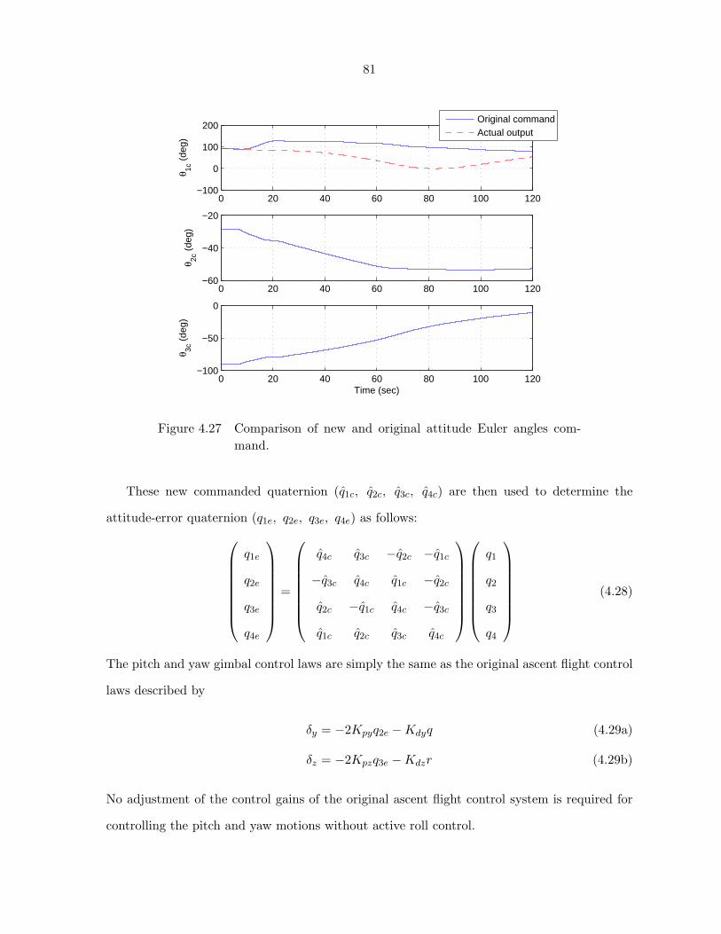
81
0 20 40 60 80 100 120−100
0
100
200
θ 1c (
deg)
Original commandActual output
0 20 40 60 80 100 120−60
−40
−20
θ 2c (
deg)
0 20 40 60 80 100 120−100
−50
0
θ 3c (
deg)
Time (sec)
Figure 4.27 Comparison of new and original attitude Euler angles com-mand.
These new commanded quaternion (q1c, q2c, q3c, q4c) are then used to determine the
attitude-error quaternion (q1e, q2e, q3e, q4e) as follows:
q1e
q2e
q3e
q4e
=
q4c q3c −q2c −q1c
−q3c q4c q1c −q2c
q2c −q1c q4c −q3c
q1c q2c q3c q4c
q1
q2
q3
q4
(4.28)
The pitch and yaw gimbal control laws are simply the same as the original ascent flight control
laws described by
δy = −2Kpyq2e −Kdyq (4.29a)
δz = −2Kpzq3e −Kdzr (4.29b)
No adjustment of the control gains of the original ascent flight control system is required for
controlling the pitch and yaw motions without active roll control.

82
0 20 40 60 80 100 120−0.5
0
0.5
1
q 1c
Original commandNew command
0 20 40 60 80 100 120−1
−0.5
0
q 2c
0 20 40 60 80 100 120−0.5
0
0.5
q 3c
Time (sec)
Figure 4.28 Comparison of new and original attitude quaternion command.
Stable closed-loop responses of the proposed approach with a modified set of desired quater-
nion can be seen from Figure 4.29 to Figure 4.32 in the event of uncontrolled roll drift. Fur-
thermore, as can be seen in Figure 4.32, the proposed control approach achieves an identical
ascent flight trajectory as the nominal ascent flight control system with active roll control.

83
0 20 40 60 80 100 120−0.5
0
0.5
q 1
0 20 40 60 80 100 120−1
−0.5
0
q 2
0 20 40 60 80 100 120−0.5
0
0.5
q 3
Time (sec)
Actual outputCommand
Figure 4.29 Quaternion for a closed-loop system stabilized by the proposedcontrol logic employing modified commanded quaternion.
0 20 40 60 80 100 120−100
0
100
θ 1 (de
g)
0 20 40 60 80 100 120−60
−40
−20
θ 2 (de
g)
0 20 40 60 80 100 120−100
−50
0
θ 3 (de
g)
Time (sec)
Actual outputCommand
Figure 4.30 Euler angles for a closed-loop system stabilized by the pro-posed control logic employing modified commanded quater-nion.

84
0 20 40 60 80 100 120−1
0
1
2
δ y (de
g)
0 20 40 60 80 100 120−1
0
1
2
δ z (de
g)
Time (s)
Figure 4.31 Gimbal angles for a closed-loop system stabilized by the pro-posed control logic employing modified commanded quater-nion.
05
10
x 104
0
5
10
x 104
0
2
4
6
8
10
12
x 104
X Position (ft)Y Position (ft)
Z P
ositi
on (
ft)
with RCSwithout RCS
Figure 4.32 Comparison of ascent trajectories: with roll control system vs.without roll control system.

85
4.5 Simple Adjustment of Control Gains
The approach presented in the preceding section provides the desired ascent flight per-
formance despite the uncontrolled roll drift. However, it requires on-board computation of
(θ1, θ2c, θ3c) to generate modified command quaternion (q1c, q2c, q3c, q4c).
In this section, we examine the feasibility of achieving pitch/yaw closed-loop stability by
simply adjusting the PD control gains without such on-board computation of (θ1, θ2c, θ3c).
We introduce a new derivative gain as
Kd = γKd (4.30)
where γ is a scale factor to be properly chosen and Kd is the original derivative gain selected
for the nominal flight conditions. And a simple PD control laws in the event of uncontrolled
roll drift are proposed as
δy = −2Kpsgn(q4e)q2e − Kdq (4.31a)
δz = −2Kpsgn(q4e)q3e − Kdr (4.31b)
As discussed in [16], the term sgn(q4e) is necessary for a quaternion-based feedback control logic
for accommodating a short angular path. In particular, such a sign change term is necessary
to avoid an undesirable 360 deg flip-over of the CLV. Some detailed analysis of this approach
is presented in this section.
From Equation. (4.11), we notice that a larger value of B = KK2d/Kp is necessary for
stability when q4e is small. The parameter K = T`/I is determined by the physical parameters
of the rocket. If Kp is decreased, then the overall loop gain of the control system is decreased,
which is not desirable. A simple way to increase the parameter B is to increase the derivative
gain Kd.
From Equation. (4.10), we have
B >1− q24e
q4e(4.32)
Kγ2K2d
Kp>
1− q24e
q4e(4.33)

86
or
γ >1Kd
√(1− q24e)Kp
q4eK(4.34)
A root locus plot of case 3 with a new derivative gain Kd = 4Kd only in the pitch channel is
shown in Figure 4.33.
−2 −1.5 −1 −0.5 0 0.5 1−0.8
−0.6
−0.4
−0.2
0
0.2
0.4
0.6
0.8
Root Locus
Real Axis
Imag
inar
y A
xis
Figure 4.33 Root locus plot for Case 3 but with a new derivative gain withγ = 4 in the pitch channel.
4.5.1 Rigid Body 6-DOF Nonlinear Simulation Results
The Matlab-based program, employing a complete set of 6-DOF nonlinear models of Ares-I
was used to validate the linear stability analysis result. The simulation results are shown in
Figure 4.34-Figure 4.37. A dispersed, but stable, ascent trajectory can be seen in Figure 4.37
for the case with a simple gain adjustment but without active roll control.
Note that after changing the control gain, structural filters also need to be adjusted. The de-
sign methodology and design tool are mentioned in Chapter 3. A design example is given here.
Flexible-body 6-DOF Nonlinear Simulation Results are similar to Figure 4.34- Figure 4.37.

87
0 20 40 60 80 100 120−1
0
1
q 1
0 20 40 60 80 100 120−1
0
1
q 2
0 20 40 60 80 100 120−1
0
1
q 3
Time (sec)
CommandActual Output
Figure 4.34 Attitude quaternion of 6-DOF nonlinear simulation withKd = 4Kd.
0 20 40 60 80 100 120−100
0
100
200
θ 1 (de
g)
0 20 40 60 80 100 120−60
−40
−20
θ 2 (de
g)
0 20 40 60 80 100 120−100
−50
0
θ 3 (de
g)
Time (sec)
Actual outputCommand
Figure 4.35 Euler angles of 6-DOF nonlinear simulation with Kd = 4Kd.

88
0 20 40 60 80 100 120−2
−1
0
1
2
δ y (de
g)
0 20 40 60 80 100 120−1
0
1
2
3
δ z (de
g)
Time (sec)
Figure 4.36 Gimbal angles of 6-DOF nonlinear simulation with Kd = 4Kd.
0 2 4 6 8 10
x 104
0
5
10
x 104
0
2
4
6
8
10
12
x 104
X Position (ft)Y Position (ft)
Z P
osi
tion (
ft)
with RCSwithout RCS
Figure 4.37 Comparison of ascent trajectories.

89
CHAPTER 5. UNDERACTUATED CONTROL PROBLEM OF AN
AXISYMMETRIC RIGID BODY
5.1 Introduction
The problem of ascent flight control in the event of uncontrolled roll drift can be generalized
as an underactuated control problem. Specifically, it is the problem of attitude stabilization
with less than three independent control torques. System equations for a rigid body rotation
can be written as follows:
p
q
r
=
Iy−Iz
Ixqr
Iz−IxIy
rp
Ix−Iy
Izpq
+
u1Ix
u2Iy
u3Iz
(5.1)
q1
q2
q3
q4
=
12
0 r −q p
−r 0 p q
q −p 0 r
−p −q −r 0
q1
q2
q3
q4
(5.2)
Note that the attitude kinematic differential equation can also be written in terms of Euler
angles as follows:
θ1
θ2
θ3
=1
cos θ2
cos θ2 sin θ1 sin θ2 cos θ1 sin θ2
0 cos θ1 cos θ2 − sin θ1 cos θ2
0 sin θ1 cos θ1
p
q
r
(5.3)

90
We have the following relationship for the rotational sequence of C1(θ1) ← C2(θ2) ←
C3(θ3)
θ1 = sgn2(q2q3 + q1q4) cos−1
1− 2(q21 + q22)√
1− 4(q1q3 − q2q4)2
(5.4a)
θ2 = sin−1−2(q1q3 − q2q4) (5.4b)
θ3 = sgn2(q1q2 + q3q4) cos−1
1− 2(q22 + q23)√
1− 4(q1q3 − q2q4)2
(5.4c)
The underactuated control problem has been dealt with [23, 24, 25, 26, 27]. Necessary and
sufficient conditions for controllability of the systems (Equation. (5.1) and Equation. (5.2) ) in
the case that the gas jet actuators yield one, two, or three independent torques are given in
[23]. Particularly, the problem of attitude stabilization of an axisymmetric (Iy = Iz) spacecraft
using two pairs of gas jet actuators is considered in [25, 26]. A new kinematic formulation is
used to derive the feedback control law.
Without loss of generality, we consider the commanded quaternion to be (0, 0, 0, 1). Then
the attitude quaternion (q1, q2, q3, q4) becomes the attitude error quaternion (q1e, q2e, q3e, q4e).
Therefore
u2 = −Kpyq2 −Kdyq (5.5a)
u3 = −Kpzq3 −Kdzr (5.5b)
Since the rigid body is assumed to be axisymmetric (Iy = Iz), we have Kpy = Kpz = Kp and
Kdy = Kdz = Kd.
Based on the analysis of Ares-I ascent flight control system in chapters 3 and 4, a modified
attitude quaternion feedback control law is derived in the next section. It can stabilize an
axisymmetric rigid body to the subsystem M (Equation. (4.20)). Moreover, a new kinematic
formulation is not needed.
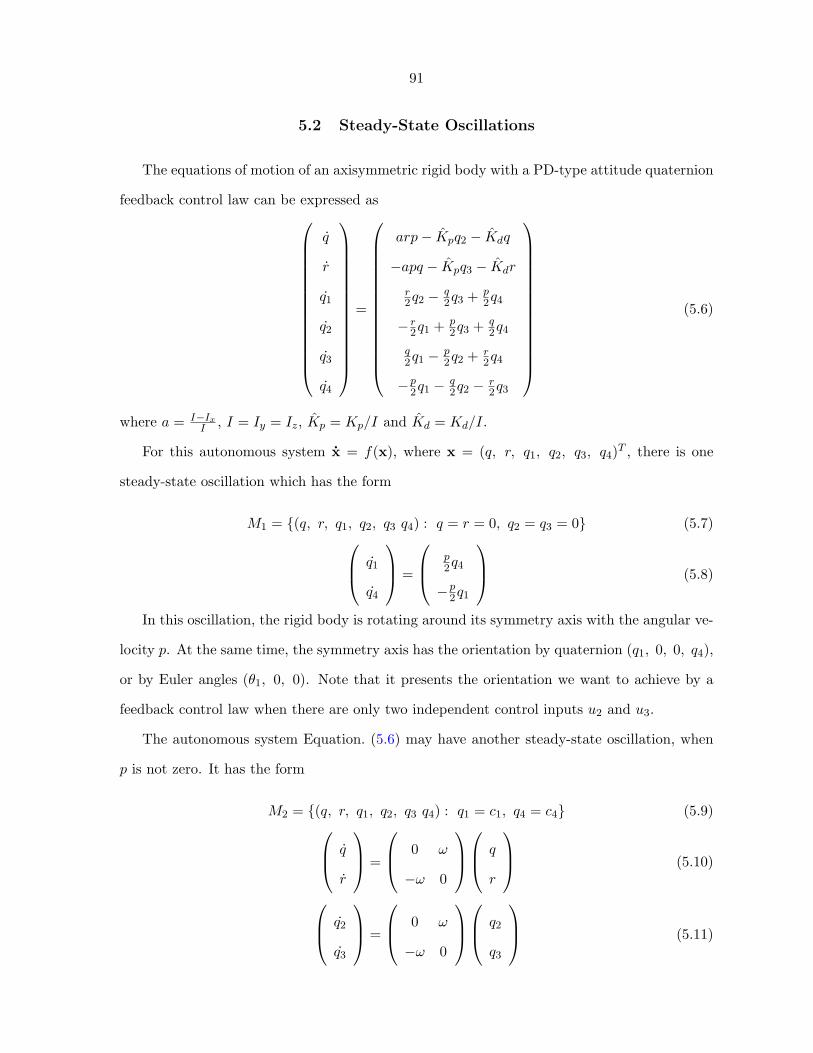
91
5.2 Steady-State Oscillations
The equations of motion of an axisymmetric rigid body with a PD-type attitude quaternion
feedback control law can be expressed as
q
r
q1
q2
q3
q4
=
arp− Kpq2 − Kdq
−apq − Kpq3 − Kdr
r2q2 −
q2q3 + p
2q4
− r2q1 + p
2q3 + q2q4
q2q1 −
p2q2 + r
2q4
−p2q1 −
q2q2 −
r2q3
(5.6)
where a = I−IxI , I = Iy = Iz, Kp = Kp/I and Kd = Kd/I.
For this autonomous system x = f(x), where x = (q, r, q1, q2, q3, q4)T , there is one
steady-state oscillation which has the form
M1 = (q, r, q1, q2, q3 q4) : q = r = 0, q2 = q3 = 0 (5.7) q1
q4
=
p2q4
−p2q1
(5.8)
In this oscillation, the rigid body is rotating around its symmetry axis with the angular ve-
locity p. At the same time, the symmetry axis has the orientation by quaternion (q1, 0, 0, q4),
or by Euler angles (θ1, 0, 0). Note that it presents the orientation we want to achieve by a
feedback control law when there are only two independent control inputs u2 and u3.
The autonomous system Equation. (5.6) may have another steady-state oscillation, when
p is not zero. It has the form
M2 = (q, r, q1, q2, q3 q4) : q1 = c1, q4 = c4 (5.9) q
r
=
0 ω
−ω 0
q
r
(5.10)
q2
q3
=
0 ω
−ω 0
q2
q3
(5.11)
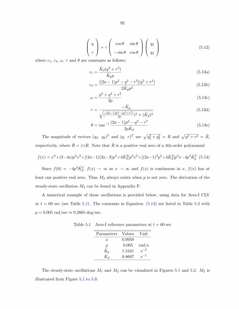
92
q
r
= τ
cos θ sin θ
− sin θ cos θ
q2
q3
(5.12)
where c1, c4, ω, τ and θ are constants as follows:
c1 =Kd(q2 + r2)
Kpp(5.13a)
c4 =[(2a− 1)p2 − q2 − r2](q2 + r2)
2Kpp2(5.13b)
ω =p2 + q2 + r2
2p(5.13c)
τ =−Kp√
( (2a−1)p2−(q2+r2)2p )2 + (Kd)2
(5.13d)
θ = tan−1 (2a− 1)p2 − q2 − r2
2pKd
(5.13e)
The magnitude of vectors (q2, q3)T and (q, r)T are√q22 + q23 = R and
√q2 + r2 = R,
respectively, where R = |τ |R. Note that R is a positive real zero of a 4th-order polynomial
f(x) = x4+(3−4a)p2x3+[(2a−1)(2a−3)p2+4K2d ]p2x2+[(2a−1)2p2+4K2
d ]p4x−4p4K2p (5.14)
Since f(0) = −4p4K2p , f(x) → ∞ as x → ∞ and f(x) is continuous in x, f(x) has at
least one positive real zero. Thus M2 always exists when p is not zero. The derivation of the
steady-state oscillation M2 can be found in Appendix F.
A numerical example of those oscillations is provided below, using data for Ares-I CLV
at t = 60 sec (see Table 5.1). The constants in Equation. (5.13) are listed in Table 5.2 with
p = 0.005 rad/sec ≈ 0.2865 deg/sec.
Table 5.1 Ares-I reference parameters at t = 60 sec
Parameters Values Unita 0.9958p 0.005 rad/sKp 1.5441 s−2
Kd 0.8607 s−1
The steady-state oscillations M1 and M2 can be visualized in Figures 5.1 and 5.2. M2 is
illustrated from Figure 5.1 to 5.9.

93
Table 5.2 Parameters of steady-state oscillation M2
Parameters Values Unitc1 0.7768 radc4 0.6242 radω 0.6994 rad/sτ −1.3963 s−1
θ −36.90 degR 0.05979 radR 0.08348 rad/s
0
0.5
1
−1
−0.5
0
0.5
1
0
0.2
0.4
0.6
0.8
1
q1
q4
z
M1 M
2
Figure 5.1 Steady-state oscillations M1 and M2 on the spherical surfaceq21 + q24 + z2 = 1.

94
−10
1
−1−0.500.51
0
0.1
0.2
0.3
0.4
0.5
0.6
0.7
0.8
0.9
1
q2q
3
z
M1
M2
Figure 5.2 Steady-state oscillations M1 and M2 on the surface of conez =
√q22 + q23.
0 10 20 30 40 50−0.01
0
0.01
p (r
ad/s
ec)
0 10 20 30 40 50−0.1
0
0.1
q (r
ad/s
ec)
0 10 20 30 40 50−0.1
0
0.1
r (r
ad/s
ec)
Time (sec)
Figure 5.3 Angular velocity of steady-state oscillation M2.

95
0 10 20 30 40 500.7769
0.7769
0.7769
q 1
0 10 20 30 40 50−0.1
0
0.1
q 2
0 10 20 30 40 50−0.1
0
0.1
q 3
Time (sec)
Figure 5.4 Attitude quaternion of steady-state oscillation M2.
0 10 20 30 40 50102
102.2
102.4
102.6
θ 1 (de
g)
0 10 20 30 40 50−10
0
10
θ 2 (de
g)
0 10 20 30 40 50−10
0
10
θ 3 (de
g)
Time (sec)
Figure 5.5 Euler angles of steady-state oscillation M2.

96
−0.1 −0.05 0 0.05 0.1−0.08
−0.06
−0.04
−0.02
0
0.02
0.04
0.06
0.08
r
q
Figure 5.6 Phase portrait of q and r of steady-state oscillation M2.
−0.06 −0.04 −0.02 0 0.02 0.04 0.06
−0.05
−0.04
−0.03
−0.02
−0.01
0
0.01
0.02
0.03
0.04
0.05
q 3
q2
Figure 5.7 Phase portrait of q2 and q3 of steady-state oscillation M2.

97
−0.1 −0.05 0 0.05 0.1−0.08
−0.06
−0.04
−0.02
0
0.02
0.04
0.06
0.08
x
y
q and rq
2 and q
3
R
|τ|R
Figure 5.8 The relation between vectors (q, r)T and (q2, q3)T of steady-s-tate oscillation M2.
0 10 20 30 40 50−10
−5
0
5
10
δ y (de
g)
0 10 20 30 40 50−10
−5
0
5
10
δ z (de
g)
Time (sec)
Figure 5.9 Gimbal angles of steady-state oscillation M2.

98
5.3 Modified Attitude Quaternion Feedback Control Law
In the last section, it was shown that there are at least two steady-state oscillations of the
autonomous system Equation. (5.6). Thus the original attitude quaternion feedback law can
not always drive Equations. (5.1) and (5.2) to M1. A new feedback control law is needed.
Define a new state variable λ, such that λ = p. A modified attitude quaternion feedback
control law has the form
u2 = −Kp[cos(λ/2)q2 + sin(λ/2)q3]−Kdq (5.15a)
u3 = −Kp[− sin(λ/2)q2 + cos(λ/2)q3]−Kdr (5.15b)
where Kp and Kd are control gains designed to stabilize a rigid body by attitude quaternion
feedback law [16]. λ is used to catch the angular velocity p.
We may obtain a new autonomous system, x = f(x) as follows:
q
r
q1
q2
q3
q4
λ
=
arp− Kp[cos(λ/2)q2 + sin(λ/2)q3]− Kdq
−apq − Kp[− sin(λ/2)q2 + cos(λ/2)q3]− Kdr
r2q2 −
q2q3 + p
2q4
− r2q1 + p
2q3 + q2q4
q2q1 −
p2q2 + r
2q4
−p2q1 −
q2q2 −
r2q3
p
(5.16)
where I = Iy = Iz, a = I−IxI , λ(0) = θ1, Kp = Kp/I and Kd = Kd/I.
5.4 Nonlinear Stability Analysis
A Lyapunov function candidate can be taken as the energy-like function
V (x) =1
2Kp
q2 +1
2Kp
r2 + [q1 − sin(λ/2)]2 + q22 + q23 + [q4 − cos(λ/2)]2 (5.17)
and V (x) = 0 when x = (0, 0, sin(λ/2), 0, 0, cos(λ/2))T , otherwise V (x) > 0.
The derivative of V (x) can be found as
V (x) = −Kd
Kp
(q2 + r2) + [q1 cos(λ/2)− q4 sin(λ/2)](p− λ) (5.18)

99
Since λ = p, we have
V (x) = −Kd
Kp(q2 + r2) ≤ 0 (5.19)
which is negative semidefinite. Detailed derivation can be found in Appendix G.
The set M1 is a positive invariant set, since
x(0) ∈M1 ⇒ x(t) ∈M1,∀t ≥ 0 (5.20)
By LaSalle’s theorem (Invariance Principle) [52], all trajectories approach M1 as t → ∞.
In addition, we have
V (x)→∞ as ‖x‖ → ∞ (5.21)
The Lyapunov function V (x) is radially unbounded. Thus the modified quaternion feedback
control law Equation. (5.15) can reorient the symmetry axis to the desired direction from an
arbitrary initial orientation. Moreover, the new control law has no restriction on the spinning
rate p, which could be an arbitrary value. Even if p keeps changing due to some disturbance
torque, the new control law still works.
5.5 Simulation Results
Two simulation cases are performed to compare the effect of original and modified quater-
nion feedback laws. Assuming that the initial spinning rate is p = 0.005 rad/sec.
Table 5.3 Simulation cases with p = 0.005 rad/sec
Case numbers Initial values (q, r, q1, q2, q3, q4) Control law1 (0, 0, 0.7769, 0.0598, 0, 0.6268, ) Original attitude quaternion feedback2 (0, 0, 0.7769, 0.0598, 0, 0.6268, ) Modified attitude quaternion feedback
The effect of M2 can be seen from Figure. 5.10 to Figure. 5.18. The trajectory converges to
M2 in a oscillation behavior. Furthermore, the modified quaternion feedback control law elim-
inates this effect. The trajectory is driven to M1, which represents the commanded orientation
of the axis of symmetry.

100
−1
−0.5
0
0.5
1
−0.50
0.5
0
0.2
0.4
0.6
0.8
1
q1
q4
z
Figure 5.10 Trajectory on the spherical surface q21 + q24 + z2 = 1 for Case1.
Start Point
Figure 5.11 Detailed trajectory on the spherical surface q21 + q24 + z2 = 1for Case 1.

101
0 50 100 150 200 250 300−0.2
−0.1
0
0.1
0.2
q (r
ad/s
ec)
0 50 100 150 200 250 300−0.2
−0.1
0
0.1
0.2
r (r
ad/s
ec)
Time (sec)
Figure 5.12 Angular velocity components q and r for Case 1.
0 50 100 150 200 250 3000.7
0.75
0.8
q 1
0 50 100 150 200 250 300−0.1
0
0.1
q 2
0 50 100 150 200 250 300−0.1
0
0.1
q 3
Time (sec)
Figure 5.13 Quaternion q1, q2 and q3 for Case 1.
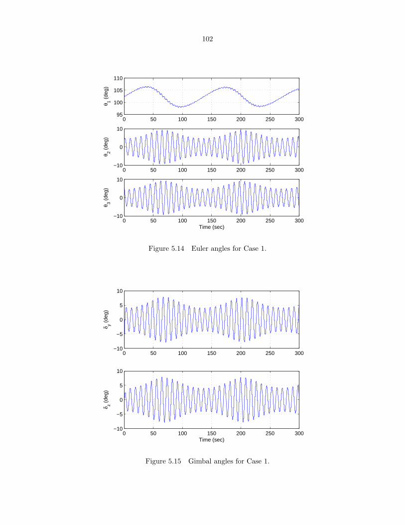
102
0 50 100 150 200 250 30095
100
105
110
θ 1 (de
g)
0 50 100 150 200 250 300−10
0
10
θ 2 (de
g)
0 50 100 150 200 250 300−10
0
10
θ 3 (de
g)
Time (sec)
Figure 5.14 Euler angles for Case 1.
0 50 100 150 200 250 300−10
−5
0
5
10
δ y (de
g)
0 50 100 150 200 250 300−10
−5
0
5
10
δ z (de
g)
Time (sec)
Figure 5.15 Gimbal angles for Case 1.

103
−0.1 −0.05 0 0.05 0.1
−0.1
−0.08
−0.06
−0.04
−0.02
0
0.02
0.04
0.06
0.08
0.1
r
q
Figure 5.16 Phase portrait of q and r for Case 1.
−0.1 −0.05 0 0.05 0.1−0.08
−0.06
−0.04
−0.02
0
0.02
0.04
0.06
0.08
q 3
q2
Figure 5.17 Phase portrait of q2 and q3 for Case 1.

104
0.75 0.76 0.77 0.78 0.79 0.8 0.81
0.6
0.605
0.61
0.615
0.62
0.625
0.63
0.635
0.64
0.645
0.65
q1
q 4
Figure 5.18 Phase portrait of q1 and q4 for Case 1.
−1
−0.5
0
0.5
1
−0.5
0
0.5
0
0.2
0.4
0.6
0.8
1
q1
q4
z
Figure 5.19 Trajectory on the spherical surface q21 + q24 + z2 = 1 for Case2.

105
Start Point
M1
Figure 5.20 Detailed trajectory on the spherical surface q21 + q24 + z2 = 1for Case 2.
0 5 10 15 20 25 30−0.04
−0.03
−0.02
−0.01
0
0.01
q (r
ad/s
ec)
0 5 10 15 20 25 30−0.02
0
0.02
0.04
0.06
r (r
ad/s
ec)
Time (sec)
Figure 5.21 Angular velocity components q and r for Case 2.

106
0 5 10 15 20 25 300.75
0.8
0.85
q 1
0 5 10 15 20 25 30−0.1
0
0.1
q 2
0 5 10 15 20 25 30−2
0
2x 10
−4
q 3
Time (sec)
Figure 5.22 Quaternion q1, q2 and q3 for Case 2.
0 5 10 15 20 25 30100
105
110
115
θ 1 (de
g)
θ1
λ
0 5 10 15 20 25 30−5
0
5
θ 2 (de
g)
0 5 10 15 20 25 30−5
0
5
10
θ 3 (de
g)
Time (sec)
Figure 5.23 Euler angles for Case 2.

107
0 5 10 15 20 25 30−6
−4
−2
0
2
δ y (de
g)
0 5 10 15 20 25 30−5
0
5
10
δ z (de
g)
Time (sec)
Figure 5.24 Gimbal angles for Case 2.

108
5.6 A Special Case
When p = 0, λ = θ1(0) is a constant. The modified attitude quaternion feedback control
law is equivalent to a quaternion command adjustment.
For a typical attitude quaternion feedback law, we have
q1e
q2e
q3e
q4e
=
q4c q3c −q2c −q1c
−q3c q4c q1c −q2c
q2c −q1c q4c −q3c
q1c q2c q3c q4c
q1
q2
q3
q4
(5.22)
The command Euler angles are (θ1c, θ2c, θ3c) = (θ1, 0, 0), where
q1c = sin(θ1c/2) cos(θ2c/2) cos(θ3c/2)− cos(θ1c/2) sin(θ2c/2) sin(θ3c/2)
q2c = cos(θ1c/2) sin(θ2c/2) cos(θ3c/2) + sin(θ1c/2) cos(θ2c/2) sin(θ3c/2)
q3c = cos(θ1c/2) cos(θ2c/2) sin(θ3c/2)− sin(θ1c/2) sin(θ2c/2) cos(θ3c/2)
q4c = cos(θ1c/2) cos(θ2c/2) cos(θ3c/2) + sin(θ1c/2) sin(θ2c/2) sin(θ3c/2)
(5.23)
The new command quaternion is
q1c = sin(θ1/2)
q2c = 0
q3c = 0
q4c = cos(θ1/2)
(5.24)
The attitude-error quaternion becomes
q1e
q2e
q3e
q4e
=
cos(θ1/2) 0 0 − sin(θ1/2)
0 cos(θ1/2) sin(θ1/2) 0
0 − sin(θ1/2) cos(θ1/2) 0
sin(θ1/2) 0 0 cos(θ1/2)
q1
q2
q3
q4
(5.25)
By the attitude quaternion feedback law, we have
u2 = −Kpq2e −Kdq = −Kp[cos(θ1/2)q2 + sin(θ1/2)q3]−Kdq (5.26a)
u3 = −Kpq3e −Kdr = −Kp[− sin(θ1/2)q2 + cos(θ1/2)q3]−Kdr (5.26b)

109
The quaternion command adjustment is a special case of the modified attitude quaternion
feedback control law, when p = 0.
q1e = − sin(θ2/2) sin(θ3/2)
q2e = cos(θ1) sin(θ2/2) cos(θ3/2) + sin(θ1) cos(θ2/2) sin(θ3/2)
q3e = cos(θ1) cos(θ2/2) sin(θ3/2)− sin(θ1) sin(θ2/2) cos(θ3/2)
q4e = cos(θ2/2) cos(θ3/2)
(5.27)
When θ2 ≈ 0, θ3 ≈ 0, we have
q1e ≈ 0
q2e ≈ cos(θ1)θ2/2 + sin(θ1)θ3/2
q3e ≈ − sin(θ1)θ2/2 + cos(θ1)θ3/2
q4e ≈ 1
(5.28)
110
CHAPTER 6. CONCLUSIONS
A set of dynamic models of the Ares-I Crew Launch Vehicle, incorporating its propulsion,
aerodynamics, guidance and control, and structural flexibility, has been described in this dis-
sertation. The results of developing a Matlab-based simulation and linearization program by
utilizing NASA’s SAVANT Simulink-based program have been discussed. The purpose of the
study was to develop an independent validation tool for the performance and stability analysis
of the ascent flight control system of the Ares-I. A linearized model of the Ares-I was obtained
as a test case of an independent validation of the ascent flight control design and analysis of
the Ares-I.
The fundamental principles of flight control analysis and design for flexible launch vehicles
have also been examined. In particular, the classical “drift-minimum” and “load-minimum”
control principles were re-examined, and the performance and stability of launch vehicle ascent
flight control with an additional feedback of angle-of-attack was demonstrated. For a typical
“non-collocated actuator and sensor” control problem of large flexible launch vehicles, non-
minimum-phase filtering of “unstably interacting” bending modes was shown to be effective
and robust.
Two distinct approaches to the ascent flight control of Ares-I in the event of uncontrolled roll
drift have been investigated. The first approach exploits the inherent versatility of a quaternion-
based attitude control system, and it only requires the desired inertial attitude quaternion to
be re-computed using the actual uncontrolled roll angle information. This approach achieved
an ascent flight trajectory identical as the nominal flight case with active roll control. The
second approach only requires a simple adjustment of the proportional-derivative gains of the
quaternion-based flight control system. The first approach is recommended for the Ares-I as

111
well as other launch vehicles in the event of no active roll control.
Finally, an undesired steady-state oscillation is found when the spinning rate is a constant.
Inspired by the method derived to stabilize a large flexible launch vehicle in the event of uncon-
trolled roll drift, a modified attitude quaternion feedback law is presented in this dissertation.
It is used to stabilize an axisymmetric rigid body by two independent control torques. By
Lyapunov’s stability analysis, it is proved that the new control law can achieve an arbitrary
orientation of the symmetry axis with arbitrary spinning rate.

112
APPENDIX A. A SUMMARY OF THE 6-DOF EQUATIONS OF
MOTION
Total force expressed in the body frame:Ftotal.xb
Ftotal.yb
Ftotal.zb
=
Faero.xb
Faero.yb
Faero.zb
+
Frkt.xb
Frkt.yb
Frkt.zb
+
Frcs.xb
Frcs.yb
Frcs.zb
(A.1)
Total force expressed in the inertial frame:Ftotal.xi
Ftotal.yi
Ftotal.zi
= CI/B
Ftotal.xb
Ftotal.yb
Ftotal.zb
(A.2)
Translational equation in the inertial frame:x
y
z
=1m
Ftotal.xi
Ftotal.yi
Ftotal.zi
+
gx
gy
gz
(A.3)
Rotational equation in the body frame:Ixx Ixy Ixz
Ixy Iyy Iyz
Ixz Iyz Izz
p
q
r
= −
0 −r q
r 0 −p
−q p 0
Ixx Ixy Ixz
Ixy Iyy Iyz
Ixz Iyz Izz
p
q
r
+
Taero.xb
Taero.yb
Taero.zb
+
Trkt.xb
Trkt.yb
Trkt.zb
+
Trcs.xb
0
0
(A.4)

113
q1
q2
q3
q4
=
12
0 r −q p
−r 0 p q
q −p 0 r
−p −q −r 0
q1
q2
q3
q4
(A.5)

114
APPENDIX B. ADDITIONAL FIGURES FROM 6-DOF SIMULATION
B.1 Atmospheric Model
900 950 1000 1050 1100 1150 12000
0.5
1
1.5
2
2.5
3
3.5
4x 10
5
Alti
tude
(ft)
Speed of Sound (ft/sec)
Figure B.1 Speed of sound

115
0 0.5 1 1.5 2 2.5 3
x 10−3
0
0.2
0.4
0.6
0.8
1
1.2
1.4
1.6
1.8
2x 10
5
Alti
tude
(ft)
Density of Air (slug/ft3)
Figure B.2 Density of air
0 20 40 60 80 100 120−10
0
10
20
Vw
.xb (
ft/se
c)
0 20 40 60 80 100 120−50
0
50
Vw
.yb (
ft/se
c)
0 20 40 60 80 100 120−100
−50
0
50
Vw
.zb (
ft/se
c)
Time (sec)
Figure B.3 Wind profile

116
0 1 2 3 4 5 6 7 8 9
x 105
−12000
−10000
−8000
−6000
−4000
−2000
0
2000
4000
6000
8000
Bas
e F
orce
(lb
)
Altitude (ft)
Figure B.4 Base force

117
B.2 Aerodynamic Coefficient
0 1 2 3 4 5
0.6
0.8
1
1.2
1.4
1.6
1.8
2
2.2
2.4
2.6
CA
Mach Number
Figure B.5 CA

118
0 1 2 3 4 5−0.26
−0.24
−0.22
−0.2
−0.18
−0.16
−0.14
−0.12
−0.1
CY
β
Mach Number
Figure B.6 CY β
0 1 2 3 4 50.1
0.12
0.14
0.16
0.18
0.2
0.22
0.24
0.26
CN
α
Mach Number
Figure B.7 CNα

119
0 1 2 3 4 51.5
2
2.5
3
3.5
4
4.5
5
5.5
CM
p α
Mach Number
Figure B.8 CMpα
0 1 2 3 4 5−5.5
−5
−4.5
−4
−3.5
−3
−2.5
−2
−1.5
CM
y β
Mach Number
Figure B.9 CMyβ

120
Rocket Parameters
0 20 40 60 80 100 1200.4
0.6
0.8
1
1.2
1.4
1.6
1.8
2
2.2x 10
6
Roc
ket W
eigh
t (lb
)
Time (sec)
Figure B.10 Rocket weight.

121
0 20 40 60 80 100 1200
0.5
1
1.5
2
2.5
3
3.5x 10
6
Thr
ust (
lb)
Time (sec)
Figure B.11 Rocket thrust.
0 20 40 60 80 100 1200
1
2x 10
6
I xx (
slug
−ft2 )
0 20 40 60 80 100 1201
2
3x 10
8
I yy (
slug
−ft2 )
0 20 40 60 80 100 1201
2
3x 10
8
I zz (
slug
−ft2 )
Time (sec)
Figure B.12 Moments of inertia.

122
APPENDIX C. LINEARIZATION RESULTS
C.1 Nonlinear 6-DOF Equations
Translational equations in the body frame:u
v
w
= −
0 −r q
r 0 −p
−q p 0
u
v
w
+ CB/I
gx
gy
gz
+1m
Faero.xb
Faero.yb
Faero.zb
+1m
T
−Tδz
Tδy
(C.1)
where
CB/I =
1− 2(q22 + q23) 2(q1q2 + q3q4) 2(q1q3 − q2q4)
2(q1q2 − q3q4) 1− 2(q21 + q23) 2(q2q3 + q1q4)
2(q1q3 + q2q4) 2(q2q3 − q1q4) 1− 2(q21 + q22)
(C.2)
Rotational equation in the body frame:Ixx Ixy Ixz
Ixy Iyy Iyz
Ixz Iyz Izz
p
q
r
= −
0 −r q
r 0 −p
−q p 0
Ixx Ixy Ixz
Ixy Iyy Iyz
Ixz Iyz Izz
p
q
r
+
Taero.xb
Taero.yb
Taero.zb
+
Trkt.xb
Trkt.yb
Trkt.zb
+
Trcs.xb
0
0
(C.3)

123
C.2 Linear Rigid-Body Model
∆u = r0∆v − q0∆w − w0∆q + v0∆r + (2gyq2c + 2gzq3c)∆q1 + (−4gxq2c + 2gyq1c − 2gzq4c)∆q2
+ (−4gxq3c + 2gyq4c + 2gzq1c)∆q3 + (2gyq3c − 2gzq2c)∆q4 +1m
∆Faero.xb
(C.4)
∆v = −r0∆u+ p0∆w + w0∆p− u0∆r + (2gxq2c − 4gyq1c + 2gzq4c)∆q1
+ (2gxq1c + 2gzq3c)∆q2 + (−2gxq4c − 4gyq3c + 2gzq2c)∆q3 + (−2gxq3c + 2gzq1c)∆q4
+1m
∆Faero.yb + (− Tm
)∆δz
(C.5)
∆w = q0∆u− p0∆v − v0∆p+ u0∆q + (2gxq3c − 2gyq4c − 4gzq1c)∆q1
+ (2gxq4c + 2gyq3c − 4gzq2c)∆q2 + (2gxq1c + 2gyq2c)∆q3 + (2gxq2c − 2gyq1c)∆q4
+1m
∆Faero.zb + (T
m)∆δy
(C.6)
Ixx 0 0
0 Iyy 0
0 0 Izz
∆p
∆q
∆r
=
b1
b2
b3
(C.7)
where the relatively small products of inertia are ignored, and
b1 = (r0Iyy − Izzr0)∆q + (Iyyq0 − q0Izz)∆r + ∆Taero.xb
+ (−cyT )∆δy + (−czT )∆δz + ∆Trcs
(C.8a)
b2 = (−r0Iyy + Izzr0))∆p+ (−(Ixxp0 + p0Izz)∆r + ∆Taero.yb + (cx −Xg)T∆δy (C.8b)
b3 = (q0Ixx − Iyyq0)∆p+ (Ixxp0 − p0Iyy)∆q + ∆Taero.zb + (Xg − cx)(−T )∆δz (C.8c)

124
∆q1 =12(q4c∆p− q3c∆q + q2c∆r + r0∆q2 − q0∆q3 + p0∆q4) (C.9a)
∆q2 =12(q3c∆p+ q4c∆q − q1c∆r − r0∆q1 + p0∆q3 + q0∆q4) (C.9b)
∆q3 =12(−q2c∆p+ q1c∆q + q4c∆r + q0∆q1 − p0∆q2 + r0∆q4) (C.9c)
∆q4 =12(−q1c∆p− q2c∆q − q3c∆r − p0∆q1 − q0∆q2 − r0∆q3) (C.9d)
Linearization of the aerodynamic forces and moments:∆Faero.xb
∆Faero.yb
∆Faero.zb
=
0 0 0
0 CY βQS/Vm 0
0 0 −CNαQS/Vm.xb
∆u
∆v
∆w
(C.10)
∆Taero.xb
∆Taero.yb
∆Taero.zb
=
0 cz −cy
−cz 0 −Xa + cx
cy Xa − cx 0
∆Faero.xb
∆Faero.yb
∆Faero.zb
+
0 0 0
0 0 CMpαQSb/Vm.xb
0 CMyβQSb/Vm 0
∆u
∆v
∆w
(C.11)
Linearization of α and β:
∆α =1
Vm.xb∆w (C.12)
∆β =1Vm
∆v (C.13)
Linearization of the thrust force and moment:∆Frkt.xb
∆Frkt.yb
∆Frkt.zb
=
0
−T∆δz
T∆δy
(C.14)
∆Trkt.xb
∆Trkt.yb
∆Trkt.zb
=
0 cz −cy
−cz 0 −Xg + cx
cy Xg − cx 0
∆Frkt.xb
∆Frkt.yb
∆Frkt.zb
(C.15)

125
Quaternion errors:
q1e
q2e
q3e
q4e
=
q4c q3c −q2c −q1c
−q3c q4c q1c −q2c
q2c −q1c q4c −q3c
q1c q2c q3c q4c
∆q1
∆q2
∆q3
∆q4
(C.16)
C.3 Linear State-Space Equations
A linearized state-space model of a rigid vehicle is described by
x = Ax + Bu
y = Cx(C.17)
where x = (∆u, ∆v, ∆w, ∆p, ∆q, ∆r, ∆q1, ∆q2, ∆q3, ∆q4)T , u = (∆Trcs, ∆δy, ∆δz)T ,
y = (2q1e, 2q2e, 2q3e, p, q, r)T ,
A =
A11 A12 A13
A21 A22 0
0 A32 A33
(C.18)
A11 =
0 r0 −q0
−r0 CY βQS/(mVm) p0
q0 −p0 −CNαQS/(mVm.xb)
(C.19)
A12 =
0 −w0 v0
w0 0 −u0
−v0 u0 0
(C.20)
A13 =
(2gyq2c + 2gzq3c) (−4gxq2c + 2gyq1c − 2gzq4c)
(2gxq2c − 4gyq1c + 2gzq4c) (2gxq1c + 2gzq3c)
(2gxq3c − 2gyq4c − 4gzq1c) (2gxq4c + 2gyq3c − 4gzq2c)
(−4gxq3c + 2gyq4c + 2gzq1c) (2gyq3c − 2gzq2c)
(−2gxq4c − 4gyq3c + 2gzq2c) (−2gxq3c + 2gzq1c)
(2gxq1c + 2gyq2c) (2gxq2c − 2gyq1c)
(C.21)

126
A21 =
Ixx 0 0
0 Iyy 0
0 0 Izz
−1
0 0 0
0 0
[− (−Xa+cx)CNαQS
Vm.xb
+CMpαQSbVm.xb
]0
[− (Xa+cx)CY βQS
Vm
+CMyβQSbVm
] 0
(C.22)
A22 =
Ixx 0 0
0 Iyy 0
0 0 Izz
−1
0 r0Iyy + Izzr0 Iyyq0 − q0Izz
−r0Iyy + Izzr0 0 −Ixxp0 + p0Izz
q0Ixx − Iyyq0 Ixxp0 − p0Iyy 0
(C.23)
A32 =12
q4c −q3c q2c
q3c q4c −q1c
−q2c q1c q4c
−q1c −q2c −q3c
(C.24)
A33 =12
0 r0 −q0 p0
−r0 0 p0 q0
q0 −p0 0 r0
−p0 −q0 −r0 0
(C.25)
B =
B1
B2
0
(C.26)
B1 =
0 0 0
0 0 −T/m
0 T/m 0
(C.27)
B2 =
Ixx 0 0
0 Iyy 0
0 0 Izz
−1
1 −cyT −czT + cyT
0 (cx −Xg)T 0
0 0 (cx −Xg)T
(C.28)

127
C =
0 0 0 0 0 0 2q4c 2q3c −2q2c −2q1c
0 0 0 0 0 0 −2q3c 2q4c 2q1c −2q2c
0 0 0 0 0 0 2q2c −2q1c 2q4c −2q3c
0 0 0 1 0 0 0 0 0 0
0 0 0 0 1 0 0 0 0 0
0 0 0 0 0 1 0 0 0 0
(C.29)
Assuming that p0 = q0 = r0 = 0, v0 = w0 = 0, θ ≈ 2q2e and Vm is a constant, then we get
the rigid-body dynamic model of Ares-I CLV in the pitch plane as follows:
α = θ +gx
Vmθ +−CNαQS
mVmα+
T
mu0δy (C.30a)
θ =−(−Xa + cx)CNαQS + CMpαQSb
Iyyα+
(cx −Xg)TIyy
δy (C.30b)
where α = ∆wVm
.
C.4 Linear Flexible-Body Model
The linear state-space equation of the Ares-I including the flexible-body modes is described
by
x = Ax + Bu
y = Cx(C.31)
where
x = (∆u, ∆v, ∆w, ∆p, ∆q, ∆r, ∆q1, ∆q2, ∆q3, ∆q4, η1, η2, η3, η4, η5, η6, η1, η2, η3, η4, η5, η6)T
(C.32)
and
A =
A 0
00 I
−Ω2 −2ζΩ
(C.33)
B =
B
0
ΦTmB1
(C.34)

128
C =
0 0 0 0 0 0 2q4c 2q3c −2q2c −2q1c
0 0 0 0 0 0 −2q3c 2q4c 2q1c −2q2c
0 0 0 0 0 0 2q2c −2q1c 2q4c −2q3c
Ψ 0
0 0 0 1 0 0 0 0 0 0
0 0 0 0 1 0 0 0 0 0
0 0 0 0 0 1 0 0 0 0
0 Ψ
(C.35)

129
APPENDIX D. ATTITUDE ERROR QUATERNION KINEMATIC
DIFFERENTIAL EQUATIONS
Equations. (2.12) and (2.46) can be written as
q =12Ωq (D.1)
qe = Qcq (D.2)
where q = (q1, q2, q3, q4)T , qe = (q1e, q2e, q3e, q4e)T , and
Ω =
0 r −q p
−r 0 p q
q −p 0 r
−p −q −r 0
(D.3)
Qc =
q4c q3c −q2c −q1c
−q3c q4c q1c −q2c
q2c −q1c q4c −q3c
q1c q2c q3c q4c
(D.4)
Note that Qc is an orthonormal matrix; that is, QcQTc = I and Q−1
c = QTc . Differentiating
Equation. (D.2) with constant commanded quaternions, we obtain
qe = Qcq (D.5)
Substituting Equation. (D.1) into Equation. (D.5), we obtain
qe =12QcΩQ−1
c qe (D.6)

130
By substituting Equations. (D.3) and (D.4) into QcΩQ−1c , we can show that QcΩQ−1
c = Ω.
An indirect approach to obtaining this relationship is provided as follows.
Let
Qc = q4cI + Q (D.7)
where
Q =
0 q3c −q2c −q1c
−q3c 0 q1c −q2c
q2c −q1c 0 −q3c
q1c q2c q3c 0
(D.8)
Note that Q and Ω are skew-symmetric matrices; that is, Q = −QT and Ω = −ΩT.
Consequently, QΩ is a symmetric matrix; that is, QΩ = (QΩ)T . Then we have
QΩ = (QΩ)T = ΩTQT = −ΩQT = ΩQ (D.9)
By using these properties, we can rewrite QcΩQ−1c as
QcΩQ−1c = QcΩQ−1
c = (q4cI + Q)ΩQ−1c (D.10)
which becomes
(q4cI + Q)ΩQ−1c = (q4cIΩ + QΩ)Q−1
c = Ω(q4cI + Q)Q−1c = ΩQcQ−1
c (D.11)
Finally, we have
QcΩQ−1c = Ω (D.12)
and
q1e
q2e
q3e
q4e
=
12
0 r −q p
−r 0 p q
q −p 0 r
−p −q −r 0
q1e
q2e
q3e
q4e
(D.13)
Note that the constant commanded quaternions are assumed here.

131
APPENDIX E. LINEAR MODEL OF UNCONTROLLED ROLL DRIFT
WITH AERODYNAMIC DISTURBANCE
v = −u0r − gxψ +CY βQS
mβ − T
mδz (E.1)
w = u0q − gxθ −CNαQS
mα+
T
mδy (E.2)
q = Mαα+Mδδy (E.3)
r = Mββ +Mδδz (E.4)
q2e =q4e
2q − q1e
2r (E.5)
q3e =q1e
2q +
q4e
2r (E.6)
where α = wu0
, β = vu0
.
When attitude error quaternion are small, we have θ ≈ 2q2e and ψ ≈ 2q3e.

132
v
w
q
r
q2e
q3e
=
CY βQSmu0
0 0 −u0 0 −2gx
0 −CNαQSmu0
u0 0 2gx 0
0 Mα/u0 0 0 0 0
Mβ/u0 0 0 0 0 0
0 0 q4e/2 −q1e/2 0 0
0 0 q1e/2 q4e/2 0 0
v
w
q
r
q2e
q3e
+
0 −T/m
T/m 0
Mδ 0
0 Mδ
0 0
0 0
δy
δz
(E.7)

133
APPENDIX F. DERIVATION OF A STEADY-STATE OSCILLATION
F.1 A Steady-State Oscillation of the Autonomous System
For this autonomous system x = f(x), we have
q
r
q1
q2
q3
q4
=
arp− Kpq2 − Kdq
−apq − Kpq3 − Kdr
r2q2 −
q2q3 + p
2q4
− r2q1 + p
2q3 + q2q4
q2q1 −
p2q2 + r
2q4
−p2q1 −
q2q2 −
r2q3
(F.1)
Assume that there is a steady-state oscillation. q1 and q4 are constants and it has the
following relation between two vectors (q, r)T and (q2, q3)T is q
r
= X
q2
q3
(F.2)
X = τ
cos θ sin θ
− sin θ cos θ
(F.3)
where |τ | is the magnitude ratio and θ is the phase shift between those two vectors. Note that
the matrix X is invertible. Therefore q2
q3
= X−1
q
r
=1τ
cos θ − sin θ
sin θ cos θ
q
r
(F.4)
Since τ and θ are constants, the relation between (q, r)T and (q2, q3)T is q
r
= X
q2
q3
(F.5)

134
Equation. (F.1) can be expressed in terms of (q, r)T , (q2, q3)T and (q1, q4)T as q
r
=
−Kd ap
−ap −Kd
q
r
+ (−Kp)
q2
q3
(F.6a)
q2
q3
=12
q4 −q1
q1 q4
q
r
+12
0 p
−p 0
q2
q3
(F.6b)
q1
q4
=12
0 p
−p 0
q1
q4
+12
r −q
−q −r
q2
q3
(F.6c)
Substituting Equation. (F.4) into Equation. (F.6a), we get q
r
=
−Kd ap
−ap −Kd
+ (−Kp)X−1
q
r
= M
q
r
(F.7)
Similarly, substituting Equation. (F.2) into Equation. (F.6b), we get q2
q3
=
12
q4 −q1
q1 q4
X +12
0 p
−p 0
q2
q3
= N
q2
q3
(F.8)
According to Equations. (F.5), (F.7) and (F.8), we obtain q
r
= X
q2
q3
= XN
q2
q3
= M
q
r
= MX
q2
q3
(F.9)
Therefore, the relation between M , N and X must be
MX = XN (F.10)
In the matrix form, we have −Kd ap
−ap −Kd
+ (−Kp)X−1
X = X
12
q4 −q1
q1 q4
X +12
0 p
−p 0
(F.11)
Note that the preceding equation is a quadratic matrix equation as follows:
XAX +BX +XC = D (F.12)

135
In the matrix form, the preceding equation can be written as
12X
q4 −q1
q1 q4
X +12X
0 p
−p 0
+
Kd −ap
ap Kd
X = (−Kp)I (F.13)
We are going to find out expressions of q1 and q4. According to the assumption that q1
and q4 are constant, we have q1
q4
=12
0 p
−p 0
q1
q4
+12
r −q
−q −r
q2
q3
=
0
0
(F.14)
therefore,
12
0 p
−p 0
q1
q4
= −12
r −q
−q −r
q2
q3
(F.15)
Substituting Equation. (F.4) into the preceding equation, we obtain
12
0 p
−p 0
q1
q4
= −12
r −q
−q −r
1τ
cos θ − sin θ
sin θ cos θ
q
r
(F.16)
The right side of the preceding equation can be simplified
12τ
r cos θ − q sin θ −r sin θ − q cos θ
−q cos θ − r sin θ q sin θ − r cos θ
q
r
=12τ
qr cos θ − q2 sin θ − r2 sin θ − qr cos θ
−q2 cos θ − rq sin θ + qr sin θ − r2 cos θ
= −q
2 + r2
2τ
sin θ
cos θ
(F.17)
Hence, q1
q4
=q2 + r2
τp
− cos θ
sin θ
= Ω
− cos θ
sin θ
(F.18)
where Ω = q2+r2
τp
F.2 Solution of the Quadratic Matrix Equation
The matrix X is the solution of the Equation. (F.13)
12X
q4 −q1
q1 q4
X +12X
0 p
−p 0
+
Kd −ap
ap Kd
X = (−Kp)I (F.19)

136
where q1
q4
= Ω
− cos θ
sin θ
(F.20)
The first term on the left side of Equation. (F.13) can be written as
12X
q4 −q1
q1 q4
X =τ2Ω2
cos θ sin θ
− sin θ cos θ
sin θ cos θ
− cos θ sin θ
cos θ sin θ
− sin θ cos θ
=τ2Ω2
0 1
−1 0
cos θ sin θ
− sin θ cos θ
=τ2Ω2
− sin θ cos θ
− cos θ − sin θ
(F.21)
The second term on the left side of Equation. (F.13) can be written as
12X
0 p
−p 0
=τ
2
cos θ sin θ
− sin θ cos θ
0 p
−p 0
=τp
2
− sin θ cos θ
− cos θ − sin θ
(F.22)
The third term on the left side of Equation. (F.13) can be written as Kd −ap
ap Kd
X =
Kd −ap
ap Kd
τ
cos θ sin θ
− sin θ cos θ
= τKd
cos θ sin θ
− sin θ cos θ
+ τap
sin θ − cos θ
cos θ sin θ
(F.23)
Substituting Equations. (F.21), (F.22) and (F.23) into Equation. (F.13), the quadratic
matrix equation becomes
(τ2Ω2
+τp
2)
− sin θ cos θ
− cos θ − sin θ
+τap
sin θ − cos θ
cos θ sin θ
+τKd
cos θ sin θ
− sin θ cos θ
= (−Kp)I
(F.24)
or
(τ(2a− 1)p
2− τ2Ω
2)
sin θ − cos θ
cos θ sin θ
+ τKd
cos θ sin θ
− sin θ cos θ
= (−Kp)I (F.25)

137
Therefore, τ and θ must satisfy the following equation τ(2a−1)p−τ2Ω2 sin θ + τKd cos θ − τ(2a−1)p−τ2Ω
2 cos θ + τKd sin θ
τ(2a−1)p−τ2Ω2 cos θ − τKd sin θ τ(2a−1)p−τ2Ω
2 sin θ + τKd cos θ
= (−Kp)I (F.26)
Note that the preceding equation can be reduced to only two equations
τ(2a− 1)p− τ2Ω2
sin θ + τKd cos θ = −Kp (F.27)
andτ(2a− 1)p− τ2Ω
2cos θ − τKd sin θ = 0 (F.28)
In the matrix form, we get τ(2a−1)p−τ2Ω2 τKd
−τKdτ(2a−1)p−τ2Ω
2
sin θ
cos θ
=
−Kp
0
(F.29)
Since Ω = q2+r2
τp , we find
τ
(2a−1)p2−(q2+r2)2p Kd
−Kd(2a−1)p2−(q2+r2)
2p
sin θ
cos θ
=
−Kp
0
(F.30)
or
τ
sin θ
cos θ
=−Kp
( (2a−1)p2−(q2+r2)2p )2 + (Kd)2
(2a−1)p2−(q2+r2)2p
Kd
(F.31)
If τ is chosen as
τ =−Kp√
( (2a−1)p2−(q2+r2)2p )2 + (Kd)2
(F.32)
Finally, solving Equation. (F.13) yields sin θ
cos θ
=1√
( (2a−1)p2−(q2+r2)2p )2 + (Kd)2
(2a−1)p2−(q2+r2)2p
Kd
(F.33)
F.3 State Equations of the Steady-State Oscillation
Substituting Equations. (F.18) and (F.33) into Equation. (F.8) yields q2
q3
= N
q2
q3
=p2 + q2 + r2
2p
0 1
−1 0
q2
q3
(F.34)

138
From Equation. (F.7) we have
M =
−Kd ap
−ap −Kd
+ (−Kp)X−1 (F.35)
According to Equations. (F.18) and (F.32), we have
M =
−Kd ap
−ap −Kd
+
√((2a− 1)p2 − (q2 + r2)
2p)2 + (Kd)2
cos θ − sin θ
sin θ cos θ
=
−Kd +√
( (2a−1)p2−(q2+r2)2p )2 + (Kd)2 cos θ ap−
√( (2a−1)p2−(q2+r2)
2p )2 + (Kd)2 sin θ
−ap+√
( (2a−1)p2−(q2+r2)2p )2 + (Kd)2 sin θ −Kd +
√( (2a−1)p2−(q2+r2)
2p )2 + (Kd)2 cos θ
(F.36)
Substituting Equation. (F.33) into the preceding equation yields
M =
0 ap− (2a−1)p2−(q2+r2)2p
−ap+ (2a−1)p2−(q2+r2)2p 0
=(p2 + q2 + r2)
2p
0 1
−1 0
(F.37)
Finally, state equations of the steady-state oscillation are listed here q2
q3
=p2 + q2 + r2
2p
0 1
−1 0
q2
q3
(F.38)
q
r
=p2 + q2 + r2
2p
0 1
−1 0
q
r
(F.39)
and q
r
= τ
cos θ sin θ
− sin θ cos θ
q2
q3
(F.40)
where
τ =−Kp√
( (2a−1)p2−(q2+r2)2p )2 + (Kd)2
(F.41)
q1
q4
=q2 + r2
τp
− cos θ
sin θ
(F.42)

139
sin θ
cos θ
=1√
( (2a−1)p2−(q2+r2)2p )2 + (Kd)2
(2a−1)p2−(q2+r2)2p
Kd
(F.43)
θ = tan−1 (2a− 1)p2 − q2 − r2
2pKd
(F.44)
Since there is another constraint
q21 + q22 + q23 + q24 = 1 (F.45)
From Equation. (F.18) we have
q21 + q24 = (q2 + r2
τp)2 (F.46)
From Equation. (F.2) we get
q2 + r2 = τ2(q22 + q23) (F.47)
Define the magnitude square of the vector (q, r)T as x
q2 + r2 = x (F.48)
and
q22 + q23 =x
τ2(F.49)
Therefore, x must satisfy the constraint
q21 + q22 + q23 + q24 = (x
τp)2 +
x
τ2= 1 (F.50)
Substituting Equation. (F.32) into the preceding equation yields
x4 +(3−4a)p2x3 +[(2a−1)(2a−3)p2 +4K2d ]p2x2 +[(2a−1)2p2 +4K2
d ]p4x−4p4K2p = 0 (F.51)
Define a function f(x) as the left side of equal sign of the preceding equation
f(x) = x4+(3−4a)p2x3+[(2a−1)(2a−3)p2+4K2d ]p2x2+[(2a−1)2p2+4K2
d ]p4x−4p4K2p (F.52)
Since x is the magnitude square of the vector (q, r)T , all real positive zeros of the function
f(x) could be x.

140
APPENDIX G. DERIVATION OF THE DERIVATIVE OF A
LYAPUNOV FUNCTION CANDIDATE
A Lyapunov function candidate is given in Equation. (5.17),
V (x) =1
2Kp
q2 +1
2Kp
r2 + [q1 − sin(λ/2)]2 + q22 + q23 + [q4 − cos(λ/2)]2 (G.1)
Expanding the square terms of quaternion, we get
V (x) =1
2Kp
q2 +1
2Kp
r2 + q21 − 2q1 sin(λ/2) + sin2(λ/2)
+ q22 + q23 + q24 − 2q4 cos(λ/2) + cos2(λ/2) (G.2)
Therefore, the Lyapunov function can be rewritten as
V (x) =1
2Kp
(q2 + r2) + 2− 2q1 sin(λ/2)− 2q4 cos(λ/2) (G.3)
The derivative of V (x) is
V (x) =1Kp
(qq + rr)− 2q1 sin(λ/2)− q1 cos(λ/2)λ− 2q4 cos(λ/2) + q4 sin(λ/2)λ (G.4)
Substituting Equation. (5.16) into the preceding equation yields the derivative of V (x)
along the trajectories of the system, then
V (x) =q
Kp
arp− Kp[cos(λ/2)q2 + sin(λ/2)q3]− Kdq
+r
Kp
−apq − Kp[− sin(λ/2)q2 + cos(λ/2)q3]− Kdr
− (rq2 − qq3 + pq4) sin(λ/2)− (−pq1 − qq2 − rq3) cos(λ/2)
− q1 cos(λ/2)λ+ q4 sin(λ/2)λ
(G.5)

141
Expanding the preceding equation yields
V (x) =apqr
Kp
− qq2 cos(λ/2)− qq3 sin(λ/2)− Kd
Kp
q2 − apqr
Kp
+ rq2 sin(λ/2)− rq3 cos(λ/2)− Kd
Kp
r2
− rq2 sin(λ/2) + qq3 sin(λ/2)− pq4 sin(λ/2) + pq1 cos(λ/2) + qq2 cos(λ/2) + rq3 cos(λ/2)
− [q1 cos(λ/2)− q4 sin(λ/2)]λ
(G.6)
Hence,
V (x) = −Kd
Kp
q2 − Kd
Kp
r2 + [q1 cos(λ/2)− q4 sin(λ/2)]p− [q1 cos(λ/2)− q4 sin(λ/2)]λ (G.7)
Finally, we obtain a compact form the the derivative of V (x)
V (x) = −Kd
Kp
(q2 + r2) + [q1 cos(λ/2)− q4 sin(λ/2)](p− λ) (G.8)
Since λ = p, we have
V (x) = −Kd
Kp
(q2 + r2) (G.9)

142
BIBLIOGRAPHY
[1] Cook, S., “Ares Project Status,” Presented at 2nd AIAA Space Exploration Conference,
December 4-6, 2006.
[2] Sumrall, P., “The Ares Projects: Progress Toward Exploration,” Presented at AIAA Space
2008 Conference, September 10, 2008.
[3] Butt, A., Popp, C. G., Pitts, H. M. and Sharp, D. J., “NASA Ares I Launch Vehicle Roll
and Reaction Control Systems Design Status,” NASA Technical Reports Server, August
2009.
[4] Norris, L., Tao, Y. C., Hall, R., Chuang, J., and Whorton, M., “Analysis of Ares-I As-
cent Navigation Options,” AIAA 2008-6290, AIAA Guidance, Navigation, and Control
Conference, Honolulu, Hawaii, August 18-21, 2008.
[5] Pinson, R. M., Schmitt, T. L., and Hanson, J. M., “Development of a Smooth Trajectory
Maneuver Method to Accommodate the Ares I Flight Control Constrains,” AIAA 2008-
6292, AIAA Guidance, Navigation, and Control Conference, Honolulu, Hawaii, August
18-21, 2008.
[6] Pitman, G. R., Inertial Guidance, New York, John Wiley and Sons, 1962, pp. 260-261.
[7] Dukeman, G. A., and Hill, A. D., “Rapid Trajectory Optimization for the Ares-I Launch
Vehicle,” AIAA 2008-6288, AIAA Guidance, Navigation, and Control Conference, Hon-
olulu, Hawaii, August 18-21, 2008.
[8] Seifert, H., Space Technology, New York, John Wiley and Sons, 1959, Chapter 4.

143
[9] Leondes, C. T., Guidance and Control of Aerospace Vehicles, New York, McGraw-Hill
Book Company, 1963, pp. 191-249.
[10] Greensite, A. L., Analysis and Design of Space Vehicle Flight Control Systems, Spartan
Books, New York, 1970, pp. 44-108, pp. 194-372.
[11] Whorton, M., Hall, C., and Cook, S., “Ascent Flight Control and Structural Interaction
for the Ares-I Crew Launch Vehicle,” AIAA 2007-1780, April 2007.
[12] Haeussermann, W., “Description and Performance of the Saturn Launch Vehicle’s Nav-
igation, Guidance, and Control System,” NASA Technical Reports Server, NASA TN
D-5869, July 1970.
[13] Frosch, J. A. and Valley, D. P., “Saturn AS-501/S-IC Flight Control System Design,”
Journal of Spacecraft, Vol. 4, No. 8, 1967, pp. 1003-1009.
[14] Blakelock, J., Automatic Control of Aircraft and Missiles, John Wiley & Sons, New York,
1991. pp. 429-437.
[15] Blackburn, T. R. and Vaughan, D. R., “Application of Linear Optimal Control and Filter-
ing Theory to the Saturn V Launch Vehicle,” IEEE Transactions on Automatic Control,
Vol. AC-16, No. 6, December 1971, pp. 799-806.
[16] Wie, B., Space Vehicle Dynamics and Control, AIAA Education Series, 1998, pp. 129-145,
pp. 381-418.
[17] Wie, B., and Barba, P. M., “Quaternion Feedback for Spacecraft Large Angle Maneuvers,”
Journal of Guidance, Control, and Dynamics, Vol. 8, No. 3, 1985, pp. 360-365.
[18] Wie, B., Weiss, H., and Arapostathis, A., “Quaternion Feedback Regulator for Spacecraft
Eigenaxis Rotations,” Journal of Guidance, Control, and Dynamics, Vol. 12, No. 3, 1989,
pp. 375-380.

144
[19] Weiss, H., “Quaternion-Based Rate/Attitude racking System with Application to Gimbal
Attitude Control,” Journal of Guidance, Control, and Dynamics, Vol. 16, No. 4, 1993, pp.
609-616.
[20] Wie, B. and Byun, K. W., “New Generalized Structural Filtering Concept for Active
Vibration Control Synthesis,” Journal of Guidance, Control, and Dynamics, Vol. 12, No.
2, 1989, pp. 147-154.
[21] Byun, K. W., Wie, B. and Sunkel, J., “Robust Non-Minimum-Phase Compensation for
a Class of Uncertain Dynamical Systems,” Journal of Guidance, Control, and Dynamics,
Vol. 14, No. 6, 1991, pp. 1191-1199.
[22] Davis, S., “Ares I-X Flight Test-The Future Begins Here,” AIAA 2008-7806, AIAA space
2008 Conference and Exposition, San Diego, California, September 9-11, 2008.
[23] Crouch, P. E., “Spacecraft Attitude Control and Stabilization: Applications of Geometric
Control Theory to Rigid Body Models,” IEEE Transactions on Automatic Control, Vol.
29, No. 4, 1984, pp. 321-331.
[24] Krishnan, H., McClamroch, N. H., and Reyhanoglu, M., “Attitude Stabilization of a Rigid
Spacecraft Using Gas Jet Actuators Operating in a Failure Mode,” IEEE Conference on
Decision and Control, Tucson, Arizona, pp. 1612-1617.
[25] Tsiotras, P., and Longuski, J. M., “Spin-axis stabilization of symmetric spacecraft with
two control torques,” Systems & Control Letters, Vol. 23, 1994, pp. 395-402.
[26] Tsiotras, P., Corless, M., and Longuski, J. M., “A Novel Approach to the Attitude Control
of Axisymmetric Spacecraft,” Automatica, Vol. 31, No. 6, 1995, pp. 1099-1112.
[27] Bymes, C.I., and Isidori. A., “On the attitude stabilization of rigid spacecraft,” Automat-
ica, Vol. 27, No. 1, 1991, pp. 87-95.

145
[28] Betts, K. M., Rutherford, R. C., McDuffie, J., Johnson, M. D., Jackson, M., and Hall, C.,
“Time Domain Simulation of the NASA Crew Launch Vehicle,” AIAA 2007-6621, August
2007.
[29] Betts, K. M., Rutherford, R. C., McDuffie, J., Johnson, M. D., Jackson, M., and Hall,
C., “Stability Analysis of the NASA Ares-I Crew Launch Vehicle Control System,” AIAA
2007-6776, August 2007.
[30] James, R. L., “A Three-Dimensional Trajectory Simulation Using Six Degrees of Freedom
with Arbitrary Wind,” NASA TN D-641, 1961.
[31] Harris, R. J., “Trajectory Simulation Applicable to Stability and Control Studies of Large
Multi-Engine Vehicles,” NASA TN D-1838, 1963.
[32] Zipfel, P. H., Modeling and Simulation of Aerospace Vehicle Dynamics, AIAA Education
Series, 1998, pp. 367-427.
[33] Stuelpnagel, J., “On the parameterization of the three-dimensional rotation group,” SLAM
Review, Vol. 6, No. 4, October 1964.
[34] Brandon, J. M., Derry, S. D., Heim, E. H., Hueschen, R. M., and Bacon, B. J., “Ares-I-X
Stability and Control Flight Test: Analysis and Plans,” NASA Technical Reports Server,
September 2008.
[35] Hall, C., Lee, C., Jackson, M., Whorton, M., West, M., Brandon, J., Hall, R. A., Jang,
J., Bedrossian, N., Compton, J., and Rutherford, C., “Ares-I Flight Control System
Overview,” AIAA 2008-6287, AIAA Guidance, Navigation, and Control Conference, Hon-
olulu, Hawaii, August 18-21, 2008.
[36] Chopra, A. K., Dynamics of Structures, Prentice Hall, New Jersey, 1995, pp. 585-600.
[37] Hoelkner, R. F., “The Principle of Artificial Stabilization of Aerodynamically Unstable
Missiles,” ABMA DA-TR-64-59, September 25, 1959.

146
[38] Hoelkner, R. F., “Theory of Artificial Stabilization of Missiles and Space Vehicles with
Exposition of Four Control Principles,” NASA Technical Reports Server, NASA TN D-
555, June 1961.
[39] Harvey, C. A., “An Alternate Derivation and Interpretation of the Drift-Minimum Princi-
ple,” NASA Contract NASw-563, MH MPG Report 1541-TR 15, Minneapolis-Honeywell,
November 22, 1963.
[40] Garner, D., “Control Theory Handbook,” NASA TM X-53036, April 22, 1964.
[41] Rheinfurth, M. H., “The Alleviation of Aerodynamic Loads on Rigid Space Vehicles,”
NASA TM X-53397, February 21, 1966.
[42] Martin, D. T., Sievers , R. F., O’Brien, R. M., and Rice, A. F., “Saturn V Guidance,
Navigation, and Targeting,” J. Spacecraft, Vol. 4, No. 7, 1967, pp. 891-898.
[43] Wie, B., and Du, W., “Analysis and Design of Launch Vehicle Flight Control Systems,”
AIAA 2008-6291, AIAA Guidance, Navigation, and Control Conference, August 2008.
[44] Doyle, J. C., Francis, B. A. and Tannenbaum A. R., Feedback Control Theory, Dover
Publication, New York, 1992, pp. 45-62.
[45] Skogestad, S. and Postlethwaite, I., Multivariable Feedback Control: Analysis and Design,
John Wiley & Sons, 2nd ed., 2005, pp. 259-338.
[46] Zhou, K., Doyle, J. C. and Glover. K., Robust and Optimal Control, Prentice Hall, New
Jersey, 1995, pp. 213-300.
[47] “Effects of Structural Flexibility on Launch Vehicle Control Systems,” NASA Technical
Reports Server, NASA SP-8036, February 1970.
[48] Balas, G. J., and Doyle, J. C., “Robustness and Performance Tradeoffs in Control Design
for Flexible Structures,” IEEE Transactions on Control Systems Technology, Vol. 2, No.
4, 1994, pp. 352-361.

147
[49] Balas, G. J., and Doyle, J. C., “Control of Lightly Damped, Flexible Modes in the Con-
troller Crossover Region,” Journal of Guidance, Control, and Dynamics, Vol. 17, No. 2,
1994, pp. 370-377.
[50] Smith, R. S., Chu, C. C., and Fanson, J. L., “The Design of H∞ Controllers for an
Experimental Non-collocated Flexible Structure Problem,” IEEE Transactions on Control
Systems Technology, Vol. 2, No. 2, 1994, pp. 101-109.
[51] Franklin, G. F., Powell, J. D., and Naeini, A. E., Feedback Control of Dynamic Systems,
5th ed., Prentice Hall, New Jersey, 2006, pp. 131-139.
[52] Khalil, H. K., Nonlinear Systems, 3rd ed., Prentice Hall, New Jersey, 2010, pp. 126-129.
[53] Sastry, S. S., Nonlinear Systems: Analysis, Stability, and Control, 1st ed., Springer, New
York, 1999, pp. 287-288.