DYNAMIC MODEL INTEGRATION AND 3D GRAPHICAL INTERFACE FOR AVIRTUAL SHIP

A THESIS SUBMITTED TOTHE GRADUATE SCHOOL OF NATURAL AND APPLIED SCIENCES

OFMIDDLE EAST TECHNICAL UNIVERSITY

BY

CANKU ALP ÇALARGÜN

IN PARTIAL FULFILLMENT OF THE REQUIREMENTSFOR

THE DEGREE OF MASTER OF SCIENCEIN

COMPUTER ENGINEERING

JANUARY 2008

Approval of the thesis

“DYNAMIC MODEL INTEGRATION AND 3D GRAPHICAL INTERFACEFOR A VIRTUAL SHIP”

submitted by Canku Alp Çalargün in partial fullfillment of the requirements forthe degree of Master of Science in Computer Engineering Department, MiddleEast Technical University by,

Prof. Dr. Canan ÖzgenDean, Graduate School of Natural and Applied Sciences

Prof. Dr. Volkan AtalayHead of Department, Computer Engineering

Assoc. Prof. Dr. Halit OguztüzünSupervisor, Computer Engineering Dept., METU

Assoc. Prof. Dr. Veysi IslerCo-supervisor, Computer Engineering Dept., METU

Examining Committee Members:

Prof. Dr. Adnan YazıcıComputer Engineering Dept., METU

Assoc. Prof. Dr. Halit OguztüzünComputer Engineering Dept., METU

Prof. Dr. M. Kemal ÖzgörenMechanical Engineering Dept., METU

Assoc. Prof. Dr. Ahmet CosarComputer Engineering Dept., METU

Assist. Prof. Dr. Tolga CanComputer Engineering Dept., METU

Date: 28/01/2008

I hereby declare that all information in this document has been obtained and

presented in accordance with academic rules and ethical conduct. I also declare

that, as required by these rules and conduct, I have fully cited and referenced all

material and results that are not original to this work.

Name, Last name : Canku Alp Çalargün

Signature :

iii

ABSTRACT

DYNAMIC MODEL INTEGRATION AND 3D GRAPHICAL INTERFACE FOR AVIRTUAL SHIP

Çalargün, Canku Alp

M.S., Department of Computer Engineering

Supervisor: Assoc. Prof. Dr. Halit Oguztüzün

Co-Supervisor: Assoc. Prof. Dr. Veysi Isler

January 2008, 120 pages

This thesis addresses the improvement of a physically based modeling simulator Naval

Surface Tactical Maneuvering Simulation System (NSTMSS), that combines different sim-

ulators in a distributed environment by the help of High Level Architecture (HLA), to be

used in naval tactical training systems. The objective is to upgrade a computer simulation

program in which physical models are improved in order to achieve a more realistic move-

ment of a ship in a virtual environment. The simulator will also be able to model the ocean

waves and ship wakes for a more realistic view. The new naval model includes a 4 degrees

of freedom (DOF) maneuvering model, and a wave model. The numerical results from real

life are used for modeling purposes to increase the realism level of the simulator. Since the

product at the end of the thesis work is needed to be a running computer code that can

be integrated into the NSTMSS system, the code implementation and algorithm details are

also covered. The comparisons between the wave models and physical models are evalu-

ated for a better real time performance. The result of this thesis shows that the integration

of a 4-DOF realistic ship model to the system improved the capability of NSTMSS to give

more data to the student officers while making maneuvers. The result also indicates that

the use of waves and ship wakes had taken the simulator to a next level in the environment

iv

perception.

Keywords: HLA, Naval Simulation, Ocean Wave Simulation, Ship Wakes

v

ÖZ

SANAL BIR GEMI IÇIN DINAMIK MODEL BIRLESTIRILMESI VE ÜÇ BOYUTLUGRAFIK ARAYÜZÜ

Çalargün, Canku Alp

Yüksek Lisans, Bilgisayar Mühendisligi Bölümü

Tez Yöneticisi: Doç. Dr. Halit Oguztüzün

Ortak Tez Yöneticisi: Doç. Dr. Veysi Isler

Ocak 2008, 120 sayfa

Bu tezde, denizsel taktik egitim sistemlerinde kullanılacak, HLA’in yardımıyla birbirinden

farklı, çesitli benzeticileri dagıtık bir ortamda birlestiren fiziksel tabanlı bir modelleme ben-

zeticisi olan NSTMSS’in gelistirilmesi konu alınır. Tezdeki amaç, bir bilgisayar benzetim

programının içindeki fiziksel modelin gelistirilerek sanal ortamdaki bir geminin hareket-

lerinin sunumunun daha gerçekçi bir gösterimini elde etmektir. Benzetici, daha gerçekçi

bir görünüm için okyanus dalgaları ve gemi dalgalarını da modelleyecektir. Deniz modeli,

4 serbestlik dereceli manevra modeli, ve dalga modeli içermektedir. Benzeticinin gerçekçi-

lik seviyesini artırmak için gerçek hayattan nümerik veriler kullanılmıstır. Tez çalısmasının

sonundaki ürün, NSTMSS’e eklenecek calısması gereken bir bilgisayar programı olması

gerektiginden, kodlama ve algoritma ayrıntıları da ele alınmıstır. Dalga modelleri ve fizik-

sel modeller arasındaki karsılastırmalar daha iyi bir gerçek zaman performansı için ele alın-

mıstır. Bu tezin sonucu, 4 serbestlik dereceli modelin NSTMSS’e eklenmesinin, NSTMSS’in

ögrencilere manevra yaparlarken daha çok bilgi verebilme kabiliyetini artırmıs oldugunu

gösterir. Tezin görsel yöndeki sonucu ise, dalgaların ve de geminin arkasında bıraktıgı

dalgaların kullanılmasının çevre algılamasında benzeticiyi bir üst seviyeye tasıdıgını da

belirtir.

vi

Anahtar Kelimeler: HLA, Deniz Simülasyonu, Okyanus Dalga Simülasyonu, Gemi Dal-

gaları

vii

To my family. . .

For being with me, all the time. . .

viii

ACKNOWLEDGMENTS

I would like to express my inmost gratitude to my supervisor Assoc. Prof. Dr. Halit

Oguztüzün. His patience, vision, sweet communication and friendly approach is the key

reason to vitalize this work. He was the one believing in me more than anybody else. It is

an honor for me to share his knowledge, wisdom and humanity.

I would also like to express my deepest gratitude and sincerest thanks to my co-supervisor

Assoc. Prof. Dr. Veysi Isler for his guidance, innovative ideas and motivation.

I would also like to express my gratitude to Okan TOPÇU for implementing the NSTMSS

application, which served as the baseline work for this thesis.

I am also indebted to Sinan Pakkan for his comments and guidance in the Naval Model

domain. I would be lost in this domain without his help.

I would like to express my heart-felt thanks to Seda, my dear wife. Without her uncondi-

tional love, joy and support, this thesis could not be completed.

I also would like to thank my parents and parents in law for their complimentary love and

support.

Finally, I would like to dedicate this work particularly to our grandmother Sadriye. I will

always remember. . .

ix

TABLE OF CONTENTS

ABSTRACT . . . . . . . . . . . . . . . . . . . . . . . . . . . . . . . . . . . . . . . . . . iv

ÖZ . . . . . . . . . . . . . . . . . . . . . . . . . . . . . . . . . . . . . . . . . . . . . . . . vi

DEDICATION . . . . . . . . . . . . . . . . . . . . . . . . . . . . . . . . . . . . . . . . . viii

ACKNOWLEDGMENTS . . . . . . . . . . . . . . . . . . . . . . . . . . . . . . . . . . . ix

TABLE OF CONTENTS . . . . . . . . . . . . . . . . . . . . . . . . . . . . . . . . . . . x

LIST OF TABLES . . . . . . . . . . . . . . . . . . . . . . . . . . . . . . . . . . . . . . . xiii

LIST OF FIGURES . . . . . . . . . . . . . . . . . . . . . . . . . . . . . . . . . . . . . . . xiv

LIST OF SYMBOLS . . . . . . . . . . . . . . . . . . . . . . . . . . . . . . . . . . . . . . xvii

CHAPTER

1 INTRODUCTION 1

1.1 Background Information . . . . . . . . . . . . . . . . . . . . . . . . . . . . 5

1.1.1 Graphics Model Background . . . . . . . . . . . . . . . . . . . . . . 5

1.1.2 Hydrodynamic Model Background . . . . . . . . . . . . . . . . . . . 7

1.2 Objective And Scope of the Thesis . . . . . . . . . . . . . . . . . . . . . . 8

1.3 Thesis Outline . . . . . . . . . . . . . . . . . . . . . . . . . . . . . . . . . . 8

2 NSTMSS SOFTWARE 10

2.1 What is HLA? . . . . . . . . . . . . . . . . . . . . . . . . . . . . . . . . . . 10

2.2 NSTMSS Objectives . . . . . . . . . . . . . . . . . . . . . . . . . . . . . . . 11

2.3 Federation Design and Frigate Federate in NSTMSS . . . . . . . . . . . . 12

3 GRAPHICAL MODEL 15

3.1 Wave Models . . . . . . . . . . . . . . . . . . . . . . . . . . . . . . . . . . 15

3.1.1 Sum of Sines Approach . . . . . . . . . . . . . . . . . . . . . . . . . 16

3.1.2 Spectrum Analysis Approach . . . . . . . . . . . . . . . . . . . . . . 21

3.2 Ocean Waves Drawing Methods . . . . . . . . . . . . . . . . . . . . . . . 25

x

3.2.1 Adaptive Surface Mesh Method . . . . . . . . . . . . . . . . . . . . 28

3.3 Dynamic Wave Simulation Configuration . . . . . . . . . . . . . . . . . . 30

3.4 Wave Shading Models . . . . . . . . . . . . . . . . . . . . . . . . . . . . . 34

3.4.1 Illumination and Shading Process . . . . . . . . . . . . . . . . . . . 34

3.4.2 Derivative Method . . . . . . . . . . . . . . . . . . . . . . . . . . . . 41

3.4.3 Vertex Neighbor List Method . . . . . . . . . . . . . . . . . . . . . . 43

3.5 Ship Wake Model . . . . . . . . . . . . . . . . . . . . . . . . . . . . . . . . 45

3.6 Cloud Simulation . . . . . . . . . . . . . . . . . . . . . . . . . . . . . . . . 49

4 THE HYDRODYNAMIC MODEL 52

4.1 Theoretical Background . . . . . . . . . . . . . . . . . . . . . . . . . . . . 52

4.1.1 Degrees of Freedom, Reference Frames and Notations . . . . . . . . 52

4.2 NSTMSS Old Hydrodynamic Model . . . . . . . . . . . . . . . . . . . . . 54

4.2.1 NSTMSS’s Simple Hydrodynamics Model . . . . . . . . . . . . . . 55

4.3 Hydrodynamic Model . . . . . . . . . . . . . . . . . . . . . . . . . . . . . 56

5 DEVELOPMENT ENVIRONMENT, ALGORITHMS AND SIMULATION RESULTS 63

5.1 Development Environment . . . . . . . . . . . . . . . . . . . . . . . . . . 63

5.1.1 COTS (Commercial of-the-shelf) . . . . . . . . . . . . . . . . . . . . 64

5.2 Algorithms . . . . . . . . . . . . . . . . . . . . . . . . . . . . . . . . . . . . 65

5.2.1 Wave Generation Algorithms . . . . . . . . . . . . . . . . . . . . . . 65

5.2.2 Wave Mesh Surface Shading Algorithms . . . . . . . . . . . . . . . 67

5.2.3 Ship Wake Generation and Drawing Algorithm . . . . . . . . . . . 72

5.2.4 Wave Drawing Algorithm . . . . . . . . . . . . . . . . . . . . . . . . 74

5.2.5 4-DOF Hydrodynamic Model Algorithm . . . . . . . . . . . . . . . 74

5.3 Main Simulation Loop . . . . . . . . . . . . . . . . . . . . . . . . . . . . . 74

5.4 Simulation Results . . . . . . . . . . . . . . . . . . . . . . . . . . . . . . . 74

5.4.1 Maneuvering Trials . . . . . . . . . . . . . . . . . . . . . . . . . . . . 78

5.4.2 Performance Tests . . . . . . . . . . . . . . . . . . . . . . . . . . . . 88

6 CONCLUSIONS AND FUTURE DIRECTIONS 96

6.1 Summary of the Thesis . . . . . . . . . . . . . . . . . . . . . . . . . . . . . 96

6.2 Conclusion . . . . . . . . . . . . . . . . . . . . . . . . . . . . . . . . . . . . 97

6.3 Future Work . . . . . . . . . . . . . . . . . . . . . . . . . . . . . . . . . . . 98

xi

A SAMPLE CODES FOR WAVE GENERATION 100

A.1 Sum of Sines Method Code . . . . . . . . . . . . . . . . . . . . . . . . . . 100

A.2 JONSWAP Wave Spectrums Finding Method . . . . . . . . . . . . . . . . 101

B SAMPLE CODES FOR WAVE SHADING 102

B.1 Derivative Method . . . . . . . . . . . . . . . . . . . . . . . . . . . . . . . 102

C SAMPLE CODES FOR WAVE MESH GENERATION 103

C.1 Adaptive Mesh Method . . . . . . . . . . . . . . . . . . . . . . . . . . . . 103

D SAMPLE CODES FOR 4-DOF HYDRODYNAMIC MODEL 105

E CONFIGURATION FILE FOR GRAPHICAL MODEL 113

F USER MANUAL 115

REFERENCES . . . . . . . . . . . . . . . . . . . . . . . . . . . . . . . . . . . . . . . . . 117

xii

LIST OF TABLES

TABLES

Table 3.1 Wave variables for different kinds of wave simulations[1] . . . . . . . 19

Table 3.2 Comparison Between Wave Generation Methods . . . . . . . . . . . . 27

Table 3.3 Tangent, Normal and Binormal Vectors . . . . . . . . . . . . . . . . . . 41

Table 4.1 DOF Description and Notations . . . . . . . . . . . . . . . . . . . . . . 53

Table 5.1 Tests of Wave Generation Methods . . . . . . . . . . . . . . . . . . . . . 94

xiii

LIST OF FIGURES

FIGURES

Figure 1.1 Lairside Maritime Simulator Bridge View . . . . . . . . . . . . . . . . 2

Figure 1.2 Lairside Maritime Simulator Outside View . . . . . . . . . . . . . . . 3

Figure 1.3 Cargo Ship from IMS . . . . . . . . . . . . . . . . . . . . . . . . . . . . 3

Figure 1.4 Ship Simulator ’07 . . . . . . . . . . . . . . . . . . . . . . . . . . . . . . 4

Figure 2.1 Meko Frigate View . . . . . . . . . . . . . . . . . . . . . . . . . . . . . 14

Figure 3.1 Sine Wave . . . . . . . . . . . . . . . . . . . . . . . . . . . . . . . . . . 17

Figure 3.2 Calm Sea with Sum of Sines Approach . . . . . . . . . . . . . . . . . . 20

Figure 3.3 Stormy Sea with Sum of Sines Approach . . . . . . . . . . . . . . . . . 20

Figure 3.4 Wave Energy Spectra of Ocean Waves . . . . . . . . . . . . . . . . . . 23

Figure 3.5 Wave Simulation with Spectrum Analysis . . . . . . . . . . . . . . . . 25

Figure 3.6 A Scene with Sum of Sines similar to JONSWAP . . . . . . . . . . . . 26

Figure 3.7 Wave Simulation with Spectrum Analysis . . . . . . . . . . . . . . . . 26

Figure 3.8 Adaptive Surface Mesh Generation Side View . . . . . . . . . . . . . . 28

Figure 3.9 Adaptive Surface Mesh Generation Top View . . . . . . . . . . . . . . 29

Figure 3.10 Adaptive Mesh Position According to the OOW . . . . . . . . . . . . 31

Figure 3.11 Appearance of the Ship Waves with Normal Mesh Method . . . . . . 32

Figure 3.12 Appearance of the Ship Waves with Incremental Mesh Method . . . . 32

Figure 3.13 Appearance of the EnviFD Federate Wave Configuration Screen . . . 33

Figure 3.14 Appearance of the Ocean Waves with Ambient Illumination . . . . . 35

Figure 3.15 Diffuse Reflection According to the Angles . . . . . . . . . . . . . . . 36

Figure 3.16 Appearance of the Ocean Waves with Ambient and Diffuse Illumination 37

Figure 3.17 Specular Reflection According to the Angles . . . . . . . . . . . . . . . 38

Figure 3.18 Appearance of the Ocean Waves with Specular Illumination . . . . . 38

xiv

Figure 3.19 Polygon Rendering Methods . . . . . . . . . . . . . . . . . . . . . . . . 40

Figure 3.20 Derivative Method Wave Shading . . . . . . . . . . . . . . . . . . . . . 43

Figure 3.21 Normal Vectors and Quad Mesh Relation . . . . . . . . . . . . . . . . 44

Figure 3.22 Point and Neighbor Triangles Relation . . . . . . . . . . . . . . . . . . 44

Figure 3.23 Vertex List Method Wave Shading . . . . . . . . . . . . . . . . . . . . . 46

Figure 3.24 A ship from above, leaving wave components and a wave component 47

Figure 3.25 Appearance of the Ship Wakes from the Ship Deck . . . . . . . . . . . 48

Figure 3.26 Appearance of the Ship Wakes from Behind . . . . . . . . . . . . . . . 49

Figure 3.27 Appearance of the Cloud Polygon . . . . . . . . . . . . . . . . . . . . 50

Figure 3.28 Appearance of the Cloud Polygons with Effect . . . . . . . . . . . . . 50

Figure 3.29 A Scene with Clouds . . . . . . . . . . . . . . . . . . . . . . . . . . . . 51

Figure 3.30 Environment Federation Cloud Density Control . . . . . . . . . . . . 51

Figure 4.1 Reference Frames and Motion Variables . . . . . . . . . . . . . . . . . 53

Figure 4.2 Main Geometric Features of a Ship . . . . . . . . . . . . . . . . . . . . 57

Figure 5.1 NSTMSS Turning Circle Roll Angle Change . . . . . . . . . . . . . . . 79

Figure 5.2 MATLAB Turning Circle Roll Angle Change . . . . . . . . . . . . . . . 79

Figure 5.3 NSTMSS Turning Circle Planar Motion Change . . . . . . . . . . . . . 80

Figure 5.4 MATLAB Turning Circle Planar Motion Change . . . . . . . . . . . . 81

Figure 5.5 NSTMSS Turning Circle Heading Angle Change . . . . . . . . . . . . 81

Figure 5.6 MATLAB Turning Circle Heading Angle Change . . . . . . . . . . . . 82

Figure 5.7 NSTMSS Turning Circle Velocity Change . . . . . . . . . . . . . . . . . 82

Figure 5.8 MATLAB Turning Circle Velocity Change . . . . . . . . . . . . . . . . 83

Figure 5.9 NSTMSS Turning Circle Shaft Speed Change . . . . . . . . . . . . . . 83

Figure 5.10 MATLAB Turning Circle Shaft Speed Change . . . . . . . . . . . . . . 84

Figure 5.11 NSTMSS Stopping Shaft Speed Change . . . . . . . . . . . . . . . . . 84

Figure 5.12 MATLAB Stopping Shaft Speed Change . . . . . . . . . . . . . . . . . 85

Figure 5.13 NSTMSS Stopping Velocity Change . . . . . . . . . . . . . . . . . . . . 85

Figure 5.14 MATLAB Stopping Velocity Change . . . . . . . . . . . . . . . . . . . 86

Figure 5.15 NSTMSS Pull Out Heading Change . . . . . . . . . . . . . . . . . . . . 86

Figure 5.16 MATLAB Pull Out Heading Change . . . . . . . . . . . . . . . . . . . 87

Figure 5.17 NSTMSS Pull Out Planar Change . . . . . . . . . . . . . . . . . . . . . 88

Figure 5.18 MATLAB Pull Out Planar Change . . . . . . . . . . . . . . . . . . . . . 89

Figure 5.19 NSTMSS Pull Out Roll Change . . . . . . . . . . . . . . . . . . . . . . 89

xv

Figure 5.20 MATLAB Pull Out Roll Change . . . . . . . . . . . . . . . . . . . . . . 90

Figure 5.21 NSTMSS Spiral Maneuver Roll Change . . . . . . . . . . . . . . . . . 90

Figure 5.22 MATLAB Spiral Maneuver Roll Change . . . . . . . . . . . . . . . . . 91

Figure 5.23 NSTMSS Spiral Maneuver Planar Change . . . . . . . . . . . . . . . . 91

Figure 5.24 MATLAB Spiral Maneuver Planar Change . . . . . . . . . . . . . . . . 92

Figure 5.25 NSTMSS Spiral Maneuver Velocity Change . . . . . . . . . . . . . . . 92

Figure 5.26 MATLAB Spiral Maneuver Velocity Change . . . . . . . . . . . . . . . 93

Figure F.1 Configuration Form of NSTMSS . . . . . . . . . . . . . . . . . . . . . . 116

xvi

LIST OF SYMBOLS

Fo : Earth-fixed reference frame−→x ,−→y ,−→z : Axes of the Earth-fixed reference frame

O : Origin of the Earth-fixed reference frame

Fb : Body-fixed reference frame−→x b,−→y b,−→z b : Axes of the Body-fixed reference frame

B : Origin of the Body-fixed reference frame

u, v, w : Translational velocities defined along the −→x b,−→y b,−→z b axes of the body-fixed ref-erence frame, respectively

p, q, r : Rotational velocities defined along the −→x b,−→y b,−→z b axes of the body-fixed refer-ence frame, respectively

X,Y, Z : Forces applied applied along the −→x b,−→y b,−→z b axes of the body-fixed referenceframe, respectively

K,M,N : Moments applied about the −→x b,−→y b,−→z b axes of the body-fixed reference frame,respectively

x, y, z : Earth-fixed coordinates of point B

φ, θ, ψ : Euler angles defining the rotation from Fo to Fb

v : 6x1 body velocity variables vector

τ : 6x1 force variables vector

η : 6x1 position and orientation variables vector

n : Actual shaft speed

nc : Commanded shaft speed

δ : Rudder deflection

δc : Commanded rudder deflection

τR : 6x1 Rigid body force variables vector

g : Gravitational acceleration

• : Dot product

× : Cross product/Multiplication

xvii

CHAPTER 1

INTRODUCTION

In today’s world, vehicle and environment simulators cover a big place in the field of

games and film industry. There are also simulators which have real-time motion bases,

visual display systems and physical models. These systems are used especially in the train-

ing of pilots and naval officers for military purposes. Since 1980s, different vendors have

developed an impressive array of simulation and training systems. These simulators were

extremely adept at training users to do their jobs as individuals or as members of a small

team. However, the ability to perform a mission as an individual does not guarantee the

ability to function as a member of a coordinated combined team, and there existed no

single simulator that offers the capabilities for team training or joint training. The impos-

sibility of one single simulator to offer all the capabilities for team training, led people to

develop technologies for networking different simulators in a common virtual play field so

that they could participate in a single virtual game. NSTMSS is one of the simulators that

serves as a distributed system for team or personal training in the naval tactical field.

The most important point in developing these simulators, either it is a single game

or a huge distributed air force simulator, is the conformance to the physical reality. So,

generating the real world effects and movement of the simulator with best accuracy is the

main target. After conforming to the excepted realism levels, the nautical simulations like

NSTMSS can be used to train young naval officers or in the design stage of the ships to

gather information about the capabilities and performance of the ship[2].

There are different kinds of naval simulators for different purposes. One example is

the "Escort Towage and Pilotage" simulator of Lairdside Maritime Centre in UK[3] which

is mainly used for which is mainly used for familiarizing towage ships to the marine pilots

with new ship types. Figure 1.1 and Figure 1.2 shows the simulator from the control room

and from the visual display system. It is easily seen in the picture that the instruments of

1

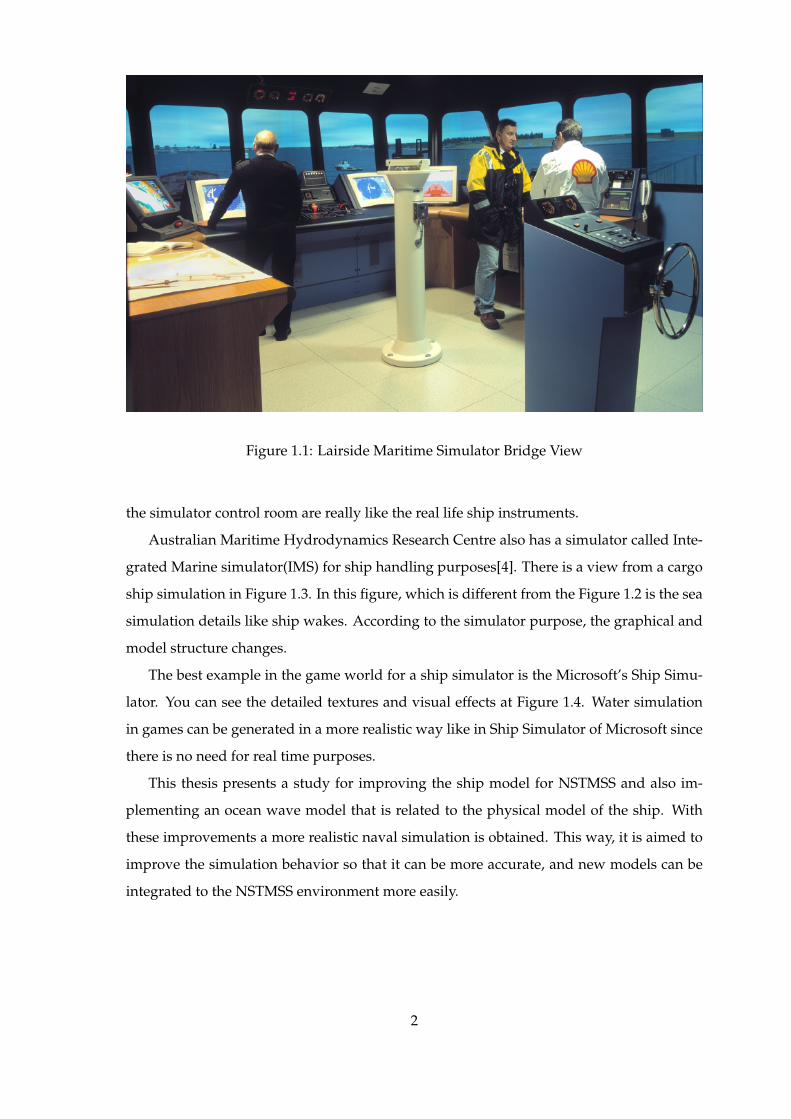
Figure 1.1: Lairside Maritime Simulator Bridge View

the simulator control room are really like the real life ship instruments.

Australian Maritime Hydrodynamics Research Centre also has a simulator called Inte-

grated Marine simulator(IMS) for ship handling purposes[4]. There is a view from a cargo

ship simulation in Figure 1.3. In this figure, which is different from the Figure 1.2 is the sea

simulation details like ship wakes. According to the simulator purpose, the graphical and

model structure changes.

The best example in the game world for a ship simulator is the Microsoft’s Ship Simu-

lator. You can see the detailed textures and visual effects at Figure 1.4. Water simulation

in games can be generated in a more realistic way like in Ship Simulator of Microsoft since

there is no need for real time purposes.

This thesis presents a study for improving the ship model for NSTMSS and also im-

plementing an ocean wave model that is related to the physical model of the ship. With

these improvements a more realistic naval simulation is obtained. This way, it is aimed to

improve the simulation behavior so that it can be more accurate, and new models can be

integrated to the NSTMSS environment more easily.

2

Figure 1.2: Lairside Maritime Simulator Outside View

Figure 1.3: Cargo Ship from IMS

3

Figure 1.4: Microsoft Ship Simulator ’07

4

1.1 Background Information

There are different fragments of a ship simulator that needs great attention during the

design and coding phase. This importance is coming from the fact that these big toys are

being used for experiencing the real life and a substitute of great vehicles that are really

hard to handle in real life situations. Time and money which is saved during the use of

these simulators are far less than the real life scenarios. That is why these vehicle simulators

needs to resemble to the real life. The simulator world keeps growing day by day and also

the need for simulators. These needs gave birth to different kinds of simulators in different

fields with variable purposes. Lots of papers and journals are published about the topic

concerning the realism levels and accuracy in real time performances. As understood from

the topics the most important pieces that is talked about at the beginning are the physical

model and the visual systems. But combining these two in great harmony to generate a

simulator that has proven itself in real-time world and realism levels is the question that

needs answers.

The use of virtual environments (VE) that resemble real life in simulators’ world has

become a must since the fast and cheaper development of graphics and hardware in com-

puter world. Especially, in military applications, it represents a possible approach to ex-

periment with new tactics and weapons, in order to interconnect training units worldwide

affordably. The most important concern while using the graphics simulation effects is to

be able to simulate the environment with most similarity to the real world but with no lack

of performance in real time. The best example about the complexities in ship simulators’

graphic interfaces is simulating the ocean wave effects. According to the detail and realism

effect the designer wants to give, the frame rate of the graphics interface decreases. Ocean

waves is not the only issue that needs attention in real time simulation of natural phenom-

ena. The weather effects, ship wakes, and the ship physical model are the most important

parts. In the following subsections background information about the mathematical and

graphical models are given.

1.1.1 Graphics Model Background

There are a significant number of literature on ocean surface simulation both in computer

graphics and oceanography. In computer graphics there are mainly three methods to sim-

ulate waves: Wave analysis is the way, first one uses. In this method wave surface is

represented by directly constructed parameter surface. In papers like [5] [6] [7] [8] [9] this

5

is the main method that is explained. For example in 1.1[10], where Ai, wi and φi changes

with time, height values (z) are found at each step.

z = f(x, y, t) =n∑i=0

Ai sin(wit+ φi) (1.1)

Because it is really hard to have fidelity in real time systems this method is suitable for

real-time simulation systems. In these kinds of equations different waves with variable

properties can be added. On the other hand, the wave breaking effects are not possible

with these kinds of algorithms.

The second way uses the physical model where hydrodynamics is the main part in solv-

ing the wave motion. These kinds of solutions, like the Navier-Strokes one, are really hard

to have in real time and needs lots of computations. Changes about the wave properties

like wave length, amplitude and speed cannot be modified dynamically. But the scenes re-

ally resembles the real physical world. The papers like [11] [12] [13] based on this physical

model solutions.

The last method is the use of particles and these particles moves according to the

rules[8] [14]. Spray and wave fraternization problems are solved but drawing particles

is a big question mark. If points or a line is chosen to simulate these particles realism effect

cannot be reached but curved surfaces are used instead. Real time performance is worse

than the other two method because of the so many calculations. Because of this, third

method is used with the other two.

Besides the ocean waves the other graphical parts that needs attention are ship wakes(the

waves a ship leaves on the ocean surface), weather effects and sky effects (cloud and sun

movements). Ship wake is really a complex phenomena. Like the ocean waves different

methods are proposed for drawing ship wakes. Because the wake pattern which is seen

around a moving ship is an extremely complex pattern, and it is very difficult to model

accurately, it is hard to find a generic solution for every ship. Recently, some papers were

published that deal with the problem from different aspects. For example in the paper

[15], parallel implementation of large eddy simulations (LES) of a ship wake using domain

decomposition technique is explained. It is explained that the accuracy of ship wake is lim-

ited by the memory of the workstation. In this example cluster of workstations are used for

simulating the wakes. Because this is not an issue in our problem a fast method is needed

to be found. Another method that is proposed can be found in [16]. Particle effects were

thought to be used in the design phase but because of the real time concerns and graphical

6

situations polygon mesh method as in this paper is used.

1.1.2 Hydrodynamic Model Background

This section of studies has an older history than the graphical part. Model based control for

steering and positioning of ships has become state-of-the-art and similar state-space tech-

niques were applied in the 1960s. Kinematics and kinetics are the two parts of the dynamic

equations for a rigid body. Kinematics is the study of motion without reference to the

forces that cause motion and kinetics, which relates the action of forces on bodies to their

resulting motions [17]. In real life, the rigid body and hydrodynamic equations of motion

for a naval vehicle are formed by a set of differential equations describing the 6-DOF. These

are surge, sway, and heave for translation, and roll, pitch, and yaw for rotation. There are

different models to represent the physics because the objectives in controlling mechanism

vary. These objectives can be divided into slow speed positioning and high speed steer-

ing. The first is called dynamical positioning (DP) and includes station keeping, position

mooring, and slow speed reference tracking. For DP the 6-DOF model is reduced to a sim-

pler 3 DOF model that is linear in the kinetic part. Such applications with references are

thoroughly described by [18] and [19]. High speed steering, on the other hand, includes

automatic course control, high speed position tracking, and path following [20], [21] and

[22]. For these applications, Coriolis and centripetal forces together with nonlinear viscous

effects become increasingly important and therefore make the kinetic part nonlinear. By the

symmetry in port-starboard, the longitudinal (surge) dynamics are essentially decoupled

from the lateral (steering; sway-yaw) dynamics and can therefore be controlled indepen-

dently by forward propulsion. Moreover, for cruising at a nearly constant surge speed and

only considering first order approximations of the viscous damping, a linear parametri-

cally varying approximation of the steering dynamics is applicable. The origin of these

types of models are traced back to [23], while [24] gave an equivalent representation. See

[25] for a historical background and [26] for a complete reference on these original models

and their later derivations.

It is needed to be emphasized that in theory most of the models are built for 6-DOF,

but the data for hydrodynamic calculations cannot be found easily in six DOF. These data

contains the hydrodynamic derivatives, damping coefficients and added mass coefficients.

The available data is mainly for 4-DOF (excluding pitch and heave). In this thesis 6-DOF

model was planed to be added but because of the lack of data and tests on the 6-DOF

7

model, 4-DOF model is added to the simulation.

1.2 Objective And Scope of the Thesis

In the preceding sections the need for naval simulators are made clear by giving details.

The objective of this thesis is to improve a naval simulator NSTMSS, in hydrodynamic

and graphical model which conforms with the real time and physical reality purposes.

There are two important goals that are needed to be accomplished. The first one is the

conformance to the real life in graphical and hydrodynamics world which means that the

reaction of the simulator to the inputs from the user needs to be as close as to the real

life. The other aim is the real time performance. Because the simulator has to work on a

standard PC the computation power is limited according to the hardware specifications.

Both of the hydrodynamic model and the graphical visual display system are in the same

application. So some precautions before designing the algorithms and writing the code are

needed to be taken. These are explained in chapter 5.

The hydrodynamics model in this thesis is taken from a master thesis project [1] which

is written in Matlabr originally in order to minimize the programming effort. One of

the parts of this thesis is to be the second stage for transferring the model to an existing

simulator NSTMSS which is designed using C++. The code is designed to be easy to modify

if another ship with different hydrodynamic model coefficients is added to the system.

The graphical improvements involves adding the ocean wave, ship wakes and some

weather effects. Letting the user change the properties and kinds of the graphical algo-

rithms, will give freedom to change the simulation according to the computational power

of the system where the system is on. The features are included or excluded according to

the necessity of the current simulation needs. Making comparisons between the methods

is also an objective for deciding the exact method for NSTMSS system.

1.3 Thesis Outline

This section will shortly describe the organization of this thesis. In this first chapter, a litera-

ture survey is presented in two subsections which are the graphical model background and

the mathematical models background. After the background information the objective and

scope is given. Chapter 2 includes brief information about the simulation system NSTMSS

into which the algorithms developed as the product of this thesis will be integrated.

8

The 3rd and 4rd chapters have the theoretical background about graphical and hydro-

dynamic model improvements respectively. Different methods for ocean wave generation

and simulating the generated waves are explained in chapter 3. 4-DOF hydrodynamic

model is studied in detailed at chapter 4.

The algorithms and the integration of them to the main system are stated in the 5th

chapter. Maneuver trials that will verify the new model and the performance tests are also

run at chapter 5.

In the final chapter, the results obtained are discussed, and future work to be accom-

plished is proposed.

9

CHAPTER 2

NSTMSS SOFTWARE

Because the integration of the hydrodynamic model and the graphical improvements to

the NSTMSS is the aim of this thesis, an introduction to the original software will be made

first of all. NSTMSS is originally designed for serving as a test bed for HLA framework

related issues and graphical advances of the system like virtual ship handling graphical

user interface design, dynamic wave models of the sea, controls that are the replicas of

the real life ship controls and natural effects like weather effect. This chapter first gives

a brief explanation to the HLA framework. In second section, the NSTMSS objectives are

summarized as items and in the last section Meko Federate, which will be the base program

for our upgrades, will be explained.

2.1 What is HLA?

From the beginning of the thesis HLA concept is being discussed to be a framework for

networked virtual environment systems and also NSTMSS is developed above that struc-

ture. In order to understand how NSTMSS uses this technology a brief introduction will

be given. The High Level Architecture (HLA) provides a common framework and ap-

proach for distributed simulations and virtual worlds to share information and capabili-

ties, to expand interoperability, and to promote reuse and extensibility. HLA is a "general

purpose architecture for distributed computer simulation systems. Using HLA, computer

simulations can communicate to other computer simulations regardless of the computing

platforms. Communication between simulations is managed by a runtime infrastructure

(RTI)" [?]. Several simulations may run on different platforms, and they may communi-

cate and interact with each other by RTI in run time. They may simply be included in the

virtual simulation environment, which is called the federation, at runtime while the other

10

simulators are already running by themselves, communicating with, affecting and being

affected by the others present in the environment. The participant simulators in the HLA

are called the federates.

HLA is not software, but an architecture that provides standard processes for defining

how distributed simulations will communicate. HLA is a set of specifications that de-

fines data objects. These standards are specified in the HLA Rules, Interface Specification

and the Object Model Template (OMT). HLA was developed under the leadership of the

Defense Modeling and Simulation Office (DMSO). The HLA Baseline Definition was com-

pleted on August 21, 1996. The Under Secretary of Defense approved it for Acquisition and

Technology (USD (A&T)) as the standard technical architecture for all DoD simulations on

September 10, 1996. The Object Management Group (OMG) adopted the HLA as the Fa-

cility for Distributed Simulation Systems 1.0 in November 1998. The HLA was approved

as an open standard through the Institute of Electrical and Electronic Engineers (IEEE) -

IEEE Standard 1516 - in September 2000. The HLA Memorandum of Agreement (MoA)

was signed and approved in November 2000.

2.2 NSTMSS Objectives

The NSTMSS project encompasses a number of objectives, which can be classified as de-

velopment objectives, principal objectives, and secondary objectives. Specifically develop-

ment objectives were focused to develop multi-user, networked, and real-time processes

from scratch with high-level 3D graphics properties in the areas:

• Design and implementation of a simple ship handling simulator.

• Design and construction of 3D virtual environment for those naval entities.

• Design and implementation of tactical picture of the operational area (As an addi-

tional federate).

The principal objectives of NSTMSS are:

• To link platform and tactical level simulations to create a realistic virtual environment

for the simulation of highly interactive naval surface operations. Multilevel train-

ing is the primary training goal for Navy’s Modeling and Simulation (M&S) Vision.

NSTMSS is combining platform and tactical level simulations to form distributed,

man-in-the-loop, interactive simulation. It also transfers the problem of interfacing

existing simulators by using HLA in lab environment.

11

• To gain experience with the HLA

• To provide reusability and interoperability. NSTMSS is based on HLA to achieve

these goals. Interoperability and reusability is two key issues for the military and

civilian Modeling and Simulation (M&S) Community [27].

• To form a test bed. HLA provides the network communication capabilities via the ser-

vices of RTI. All the functionality of the recently proposed HLA and its components

(RTI, rules and Object Model Template OMT) are being tested by the development of

NSTMSS. NSTMSS can serve as a test bed:

– For interoperability and performance issues of HLA,

– For fine tuning RTI management service parameters, such as tick() function,

– For empirical evaluation of dead reckoning algorithms,

– For testing the efficiency of multicast protocols over a Networked Virtual Envi-

ronment (NVE),

– For equipment simulators, such as RADAR simulators.

• To gain the full benefits of team training in the virtual environment. Like other mil-

itary operations, a naval surface operation involves planning, on time carrying out,

and evaluation phases. A naval surface operation is carried out by the participation

of planning officers, ships and navy-shore facilities. The System will also create an

environment for naval surface actions which new tactics, operations and formations

can be evaluated and tested as well as the present ones can be practiced and analyzed.

There are some secondary objectives, which we may also call "By-Products". The intended

scope of this project will include, but not be limited to, the following additional objectives:

• A reusable object library (C++ API) is constructed.

• Second, Federation Development and Execution Process (FEDEP) methodology im-

provement is achieved by a graphical federation design notation and by iterative and

incremental development approach.

2.3 Federation Design and Frigate Federate in NSTMSS

A typical distributed training system is composed of federates for human players who

are being trained, environment generation federates which form the play field, instructor

12

federates which tell these what and how to play and observer federates which collect infor-

mation about the underlying communication infrastructure. The frigate federates are the

ship simulation softwares that can be combined in a networked environment.

Meko whose name is coming from the Meko type frigates, is the part where the im-

provements will be integrated. The users (Officers and student officers) can interact with

the software from the user interface of the federate by giving inputs like shaft speed and

rudder angles. They get the feedback from the bridge view of the ship, instrument states

and present course of the ship. The user may view the position of the ship in terms of

latitude and longitude coordinates, view the other ships in the federation in the radar dis-

play, and the environment by the bridge windows and communicate with the users of the

other ships, when using the simulator brought into the virtual environment by the Meko

federate. A view of the Meko federate user interface can be seen in Figure 2.1.

In the original design of NSTMSS, rather than ship handling the aim of the training is

on formation maneuvering. Because of that the disturbance forces from the environment

are not the main importance. In case of this assumptions the ships are assumed to be sailing

in still sea where no wind, wave or ocean current effects are present.

13

Figure 2.1: Meko Frigate view from the bridge

14

CHAPTER 3

GRAPHICAL MODEL

In this chapter the improvements that are about the graphical interface of the system are

explained in detail. First of all the wave models are discussed in section 3.1 and in section

3.2 the drawing details of these wave models are described. For a more realistic view the

lighting and shading mechanisms should conform with the real life situations. So in the

following section 3.4 the shading models are discussed in detail. The other simulation

issue in ocean and ship interaction simulation is the ship wake modeling. The section

3.5 discusses this topic and explains the way that is used. The last section gives a brief

explanation of the cloud simulation that is added to the NSTMSS system.

3.1 Wave Models

As mentioned in the preceding chapters, real time performance of a simulator is the most

important issue in the design and coding phase. Different kinds of wave models according

to their reality levels can be generated. In this thesis two wave models are tried and com-

pared according to our simulation needs. The first one is from the first group of waves that

is discussed in the section Graphics model background of chapter 1. A height field above

the sea level is generated and summation of sine waves method is used to get the current

time wave point positions [28]. The second method that is used based on the spectrum

analysis in solving the wave motion. JONSWAP wave spectrum [1] will be used in the

wave generation phase. There is also another issue about waves which is the finding of the

normals of each point on the wave surface. This is needed because of the shading issues of

the waves. Methods from different sources are explained and compared about shading of

the wave mesh generated.

15

3.1.1 Sum of Sines Approach

Besides the deep ocean simulations which are used in some movies and computer games

[5], real-time models for ocean vehicle simulations are needed. One of these approaches

has been developed by Miguel Gomez [29] which is about an implicit way of finding height

fields. But the disadvantage in this solution is that there is a need to hold two height field

meshes to calculate the current one. Also, to calculate the next position for each vertex the

neighbor information is needed.

Mark Finch’s solution [28] to the real-time wave simulation which forms a baseline for

this method has lots of advantages to the other wave models. These are:

• For position updates the neighbor information is not needed.

• If a developer is using the GPU and vertex shader for coding because there is no need

for neighbor information, it is easy to implement by using the graphics hardware.

• All the properties of a wave can be parameterized and user will have a full control

over it in real-time.

• Normal can be found by using just the local vertex data. It makes it possible to use

the vertex shader for implementation. If neighbor data is wanted to be used it is also

possible. In this paper they are compared according to the CPU usage and real-time

performance.

• It is easy to change the mesh dimensions and scale the wave data.

• Algorithm can be used with same efficiency for high wind waves and small frequency

waves.

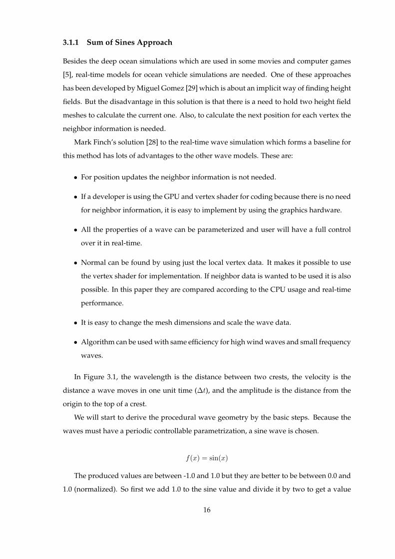
In Figure 3.1, the wavelength is the distance between two crests, the velocity is the

distance a wave moves in one unit time (∆t), and the amplitude is the distance from the

origin to the top of a crest.

We will start to derive the procedural wave geometry by the basic steps. Because the

waves must have a periodic controllable parametrization, a sine wave is chosen.

f(x) = sin(x)

The produced values are between -1.0 and 1.0 but they are better to be between 0.0 and

1.0 (normalized). So first we add 1.0 to the sine value and divide it by two to get a value

16

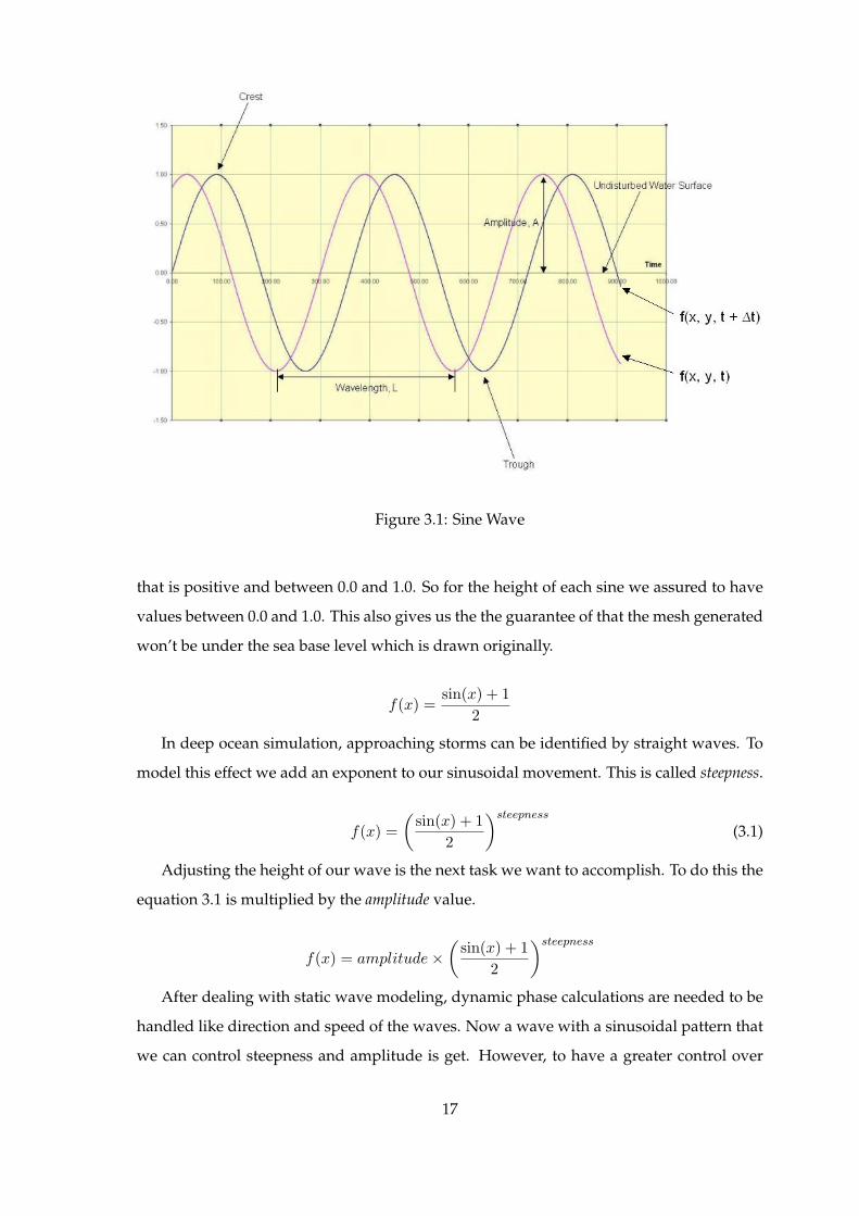
Figure 3.1: Sine Wave

that is positive and between 0.0 and 1.0. So for the height of each sine we assured to have

values between 0.0 and 1.0. This also gives us the the guarantee of that the mesh generated

won’t be under the sea base level which is drawn originally.

f(x) =sin(x) + 1

2

In deep ocean simulation, approaching storms can be identified by straight waves. To

model this effect we add an exponent to our sinusoidal movement. This is called steepness.

f(x) =(

sin(x) + 12

)steepness(3.1)

Adjusting the height of our wave is the next task we want to accomplish. To do this the

equation 3.1 is multiplied by the amplitude value.

f(x) = amplitude×(

sin(x) + 12

)steepnessAfter dealing with static wave modeling, dynamic phase calculations are needed to be

handled like direction and speed of the waves. Now a wave with a sinusoidal pattern that

we can control steepness and amplitude is get. However, to have a greater control over

17

the surface the speed and direction of the wave as well as the wavelength are needed to be

taken into account. Since a 2-dimensional height field is simulated, the movement in each

direction is needed to be considered. To accomplish this x,y position is projected onto a

wave direction vector using a dot product. For simplicity we assume the direction vector

is parallel to the flat surface and therefore has no z component. Recall the result of a dot

product between two vectors is a scalar value which is denoted as S.

S = Dir(x, y) • Pos(x, y)

Next, the frequency of the wave must be taken into account. It is known from physics

that the wavelength relates to frequency as frequency = 2*π/wavelength. Therefore the wave-

length can be used as input and frequency will be generated by this function. Since this is

wanted to influence the periodicity of values delivered to sin function, it is incorporated

into the function as below.

S = Dir(x, y) • Pos(x, y)× frequency

A wave that takes the wavelength and direction into account to determine the position

is generated. If the velocity of the wave can be added than waves will actually move. From

the physics it is known that the phase constant ϕ is related to velocity by the equation ϕ

= velocity × frequency where ϕ = velocity × (2π/wavelength). The equation is changed as

follows where t is time.

S = Dir(x, y) • Pos(x, y)× frequency + t× ϕ

In summary, we now have a function that takes into account wavelength, amplitude,

velocity, direction, position, steepness, and amplitude:

f(x, y, t) = amplitude×(sin(S) + 1

2

)steepness, where (3.2)

S = Dir(x, y) • Pos(x, y)× frequency + t× ϕ

Wave Composition

According to the complexity level of the simulation the number of sine waves can be

changed. If a true deep ocean wave surface is needed than a greater degree of variabil-

ity is needed. There are multiple waves that are generated from different sources and they

18

Table 3.1: Wave variables for different kinds of wave simulations[1]

Sea State Amplitude

Calm (Glassy) 0

Calm (Rippled) 0 - 0.1

Smooth (wavelets) 0.1 - 0.5

Slight 0.5 - 1.25

Moderate 1.25 - 2.5

Rough 2.5 - 4

Very Rough 4 - 6

High 6 - 9

Very High 9 - 14

Phenomenal 14+

interfere with each other. Also their directions can be different from one another. They all

together form peaks, troughs, and some vibrate. To simulate this we will take into account

several waves by summing their positions at any point in our simulation. We have chosen

to limit the number of sine waves to 4 and found that this provides an adequate amount of

variability. To simulate the height of a position (x,y) we have the equation 3.3.

heigth(x, y, t) =4∑i=1

f(x, y, t) (3.3)

In Figure 3.2 and Figure 3.3 an ocean surface with slight waves and a stormy sea with

very rough waves can be seen respectively. In table Table 3.1 the amplitude variable for

drawing the wave simulations for different sea states are given. In this table, the variable

does not have any unit where an amplitude unit is equal to 1 performer unit. Since the

simulated scenes may differ according to the mesh size and the quad unit sizes that form

the mesh, the units cannot be specified. The amplitude values are given for a 30x30 mesh

which is formed with the quads that have edges of 10 units in a performer scene. To clarify

the unit perception in a performer scene, the Meko frigate in NSTMSS project has a length

of 108 units. According to the mesh generated, the sine wave variables can be changed

rationally to have the same effect in scenes with different drawing properties. It is impor-

tant to note that, the variables wavelength, steepness, speed should also be changed in

harmony with amplitude to simulate ocean waves with different properties.

19

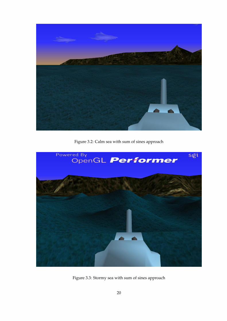
Figure 3.2: Calm sea with sum of sines approach

Figure 3.3: Stormy sea with sum of sines approach

20

3.1.2 Spectrum Analysis Approach

This wave model is much more complex than the first method and this is actually used to

reflect the wave effect to the ship motion model. As you will see in the following section

the calculation of the height map is much mote complex than the first method.

As explained before, this model is taken from the master thesis [1]. The mathematical

representation of the formula is from [30] and [31]. As in the first sum of sines method, in this

method also the wave elevation is given as a function of time and space and it is formed as

the sum of sinusoids with random phases. The below formula will make the explanation

clearer:

ζ(x, y, t) =N∑i=1

Aicos(ωit− ki(xsin(χ) + ycos(χ)) + φi)

+N∑i=1

12kiA

2i cos2(ωit− ki(xsin(χ) + ycos(χ)) + φi)

+ f(A3i ))

(3.4)

Vega Marine module [32] of Vega Prime simulation framework uses the same approach

for wave generation. But only the first order term is used and also the coefficient for each

wave component is 0.112Hs in Vega Marine module. Once a spectrum is found by gener-

ating the frequency content of ocean waves, then a finite number of sinusoids can model

ocean waves. The wave height function ζ, is a function of xy-grid which is parallel to the

reference frame and time. In this formula the 1st order terms represents the oscillatory

motion and the 2nd order terms are for drift forces.

In this section just the wave elevation algorithm will be discussed other than the wave

forces acting on the ship. The hydrodynamics model section deals with forces generated.

To start with, the spectral density is computed according to the assumptions and param-

eters selected. The spectrum analysis section has the details about this part and it will be

explained in detail. After the spectrum is available, the division of it into N parts along

the frequency axis where the width of each interval is ∆ω. After that S(ωi)’s are calcu-

lated which will be used in the calculation of Ai’s where the ωi’s are the randomly selected

frequencies from each of the intervals. Ai’s are calculated according to the equation below:

21

Ai =√

2S(ωi)∆w (3.5)

Also the wave numbers are found as below:

ki =ω2i

g(3.6)

Note that in the equation 3.6 water depth is thought to be infinite because the actual

equation is ω2i = kig tanh(kid) where d is the water depth. It is good to use equation 3.6

where d/λi > 1/2. λi is the wavelength of the ith component.

So the wave elevation formula can be written as below in a more general form where n

is the depth of approximation:

ζ(x, y, t) =n∑j=1

N∑i=1

kj−1i Aji cos(ωit− ki(xsin(χ) + ycos(χ)) + φi) (3.7)

In equation 3.7 χ is the heading of the wavefront on the grid determined by the x and

y coordinates and φi’s are the uniformly distributed random phase angles for each sinu-

soidal wave components.

Finding Wave Spectral Densities

The wave spectrum types are explained in the master thesis [1] in detail. Since JONSWAP

spectrum is the main one that is used in this thesis it will be mentioned in this section.

Before that a summary should be given about spectrum analysis and their source of data.

Winds, earthquakes, and tide can the source of waves. Figure 3.4 which is taken from

[33] shows the frequency content of ocean waves. In this thesis only the waves that are

generated by wind will be studied.

In equation 3.5 the wave amplitudes are found by using the frequency spectra. For

a long period of time data is gathered and some formulations based on these are devel-

oped. By these formulas power spectral densities are found and in this section one of these

spectrum analysis methods will be discussed. To make the terminology clearer some data

about the concept should be given first. The factors that affect the shape of the wave are

wind velocity and the effectiveness of the wind. The main source of the effectiveness is

called Fetch which is the distance that the wind is able to blow along over the sea surface.

From the storms that are far away from the wave point generates swells and these are the

decaying waves. So one directional waves cannot be the situation in anytime. Also the sea

22

Figure 3.4: Wave Energy Spectra of Ocean Waves

23

depth has a big role in the shape of the spectrum. Shallow waters have higher frequency

waves because of that.

JONSWAP SPECTRUM : Some assumptions are made before using the spectrum anal-

ysis methods. With using the JONSWAP one we assume that the sea:

• is non-fully developed.

• has finite water depth

• has limited fetch

This spectrum is widely used in literature and the name comes from Joint North Sea Wave

Project.

S(ω) : Spectral density of the wave component with frequency ω

Unit for the wave spectrums is [m2s].

S(ω) = 155H2s

T 41ω

5− exp

(944T 4

1ω4

)(γ)Y

where

Y = exp

[−(

0.191 · ω · T1 − 1√2σ

)2]

σ =

0.07 for ω ≤ 5.24/T1

0.09 for ω > 5.24/T1

For the other representation of this spectrum you can see [1].

This method is not for real time systems because it needs much more computation than

the first sum of sines method and the properties cannot be changed on the run. Since the

height levels are found for a time interval before the simulation started, the users need to

24

Figure 3.5: Wave simulation with spectrum analysis

wait before starting the training session and the properties like wind speed and spectrum

properties cannot be changed. In Figure 3.5 and Figure 3.7 there are two images with

different wave properties which are created by using JONSWAP spectrum method. In

Figure 3.7 the maximum frequency is 6 where the same variable is 2 in the first picture. In

the chapter 5 these solution methods will be studied in more detail.

In Figure 3.6 you can see a scene that is nearly same with the JONSWAP one in Fig-

ure 3.5. As long as the parameters are set correctly in sum of sines method users can get

equal results with the spectrum analysis generated ocean waves.

To talk about the superiorities on each other of these two methods will be appropriate

here. In Table 3.2 the pros and cons are listed.

3.2 Ocean Waves Drawing Methods

As it is mentioned before, trying to draw the natural phenomena closer to real life in VE en-

vironments is the hardest task because of the lack of the computation speed and resources.

It is the same as the ocean surface because ocean surface is a large area, and a high mesh

resolution is needed for sampling the waves. Therefore, different methods were used to

25

Figure 3.6: A scene with sum of sines similar to JONSWAP

Figure 3.7: Wave simulation with spectrum analysis

26

Table 3.2: Comparison Between Wave Generation Methods

Properties Spectrum Analysis Sum of Sines

Usability with Long Initialization period No initialization step

real time No need for calculation Needs calculation during

during simulation simulation more complex with

the size of the wave mesh

Wave Property Handling Cannot be changed in The properties can be changed

simulation time during simulation

Realism Level These are according to real Imaginary sinusoidal

data which are collected signals which does not have

for decades any realism level

Variability Number of waves can be much If number of waves gets

more larger than the sine larger it effects the

method. Just the frame number dramatically

initialization time because of the dynamic

changes. This does not calculation of wave

effect the simulation time heights

27

Figure 3.8: Adaptive surface mesh generation side view

simulate ocean surface to give a better real life perception. For instance, in [34] an adaptive

mesh method is applied for simulating the ocean surface of a multi-channel marine simu-

lator. On the other hand, in [35] another adaptive surface mesh method in a different way

is used. In this thesis a different kind of adaptive surface drawing method will be used and

it will be compared to the normal mesh drawing methods.

3.2.1 Adaptive Surface Mesh Method

Instead of drawing a predetermined, regularly sampled region of the ocean surface, the

regions that the OOW’s view at, can be sampled and a continuous LOD (Level of Detail)

mesh is used for that purpose. Because of the large visible ocean surface area, the wave

simulation cannot be applied on all the ocean surface totally. On the other hand, a high

mesh resolution is needed in regions close to the eye-point, and a low mesh resolution is

enough for the distant regions. So a mesh with continuous LOD is created and the position

of the quads on the mesh are changed according to the position and the view angle of the

officer on deck.

28

Figure 3.9: Adaptive surface mesh generation top view

The most important point is [35] creating the mesh which represents the ocean surface

such that every grid shows the same area on the screen. After dividing the screen into

the equal surface parts these are projected on the plane where the modeling of the waves

are done. The mesh points after dividing the plane into nxn quads, as seen on Figure 3.8

and Figure 3.9, are adequate for representing the ocean surface properly. The field of view

(FOV) angle is also taken into account while dividing the plane. According to the FOV

angle and the number of the points that are generating the mesh (in Figure 3.9 it is n) the

points generating the mesh are automatically initialized. This process will be explained in

chapter 5 by a pseudo code in detail.

As you can see in Figure 3.10 the officer on the deck can change his heading according to

the inputs from the user. While turning the mesh also needs to move to the heading area of

the OOW. This is done by moving all the points of the mesh relatively to the standing point

and the heading angle of the OOW. X and Y points of each vertex in the mesh is recalculated

29

at the beginning of each loop according to the heading and the position of the officer. This

is done by initializing the position mesh point values relative to the officer’s starting point.

According to those relative distances and the heading angle the new positions at each step

are calculated and the wave simulation algorithms are run on those new vertex values.

There is an important point that should be noted. As it is explained in sections of wave

generation, the wave directions are given to the wave point calculation algorithms. Since

the directions are given first according to a steady mesh vertex group, with the change of

the position of the vertex points the direction is needed to be calculated again by using the

heading of the OOW. If the direction is not changed than with the change of the position

mesh points the direction also changed in a wrong way. Using a method that enables us

to simulate the same direction effect on a moving vertex group is needed. Because the

direction of the wave is a vector, if it is multiplied by a rotation matrix whose rotation

value is equal to the angle of heading of the user, the problem is solved easily.

Use of this method induces a continuous shift of the mesh over the ocean surface, an

adequate resolution being maintained everywhere in the computed image. We can note

that this sampling strategy is made possible by the continuously moving nature of the

ocean surface: using a similar approach for rendering a landscape, for example, would

produce artifacts since the camera motion induces a shift in the sampling locations. This

sampling artifact actually takes place, but is hidden by the waves animation.

In Figure 3.11 and Figure 3.12 you can see the difference of the horizon view. In the

normal mesh drawing method the horizon passing from wave mesh to the normal sea

surface is really distinct. But in adaptive surface mesh method because the quads gets

larger as the distance from the user extends, the farthest distance a quad can appear is

longer than in the normal mesh drawing method. Therefore, the visualization of the surface

mesh with adaptive method is more pleasant to the user’s eye. It is important to note that,

to increase the quad numbers in the normal mesh drawing method won’t be a solution

because of the increasing computation time in the wave elevation process. If the number

of quads increase the complexity of the simulation will increase with the square of the

difference and affect the frame frequency values.

3.3 Dynamic Wave Simulation Configuration

As stated in second chapter NSTMSS is a networked simulation system that uses HLA. One

of the federates of NSTMSS is the Environment federate and it is used to configure mainly

30

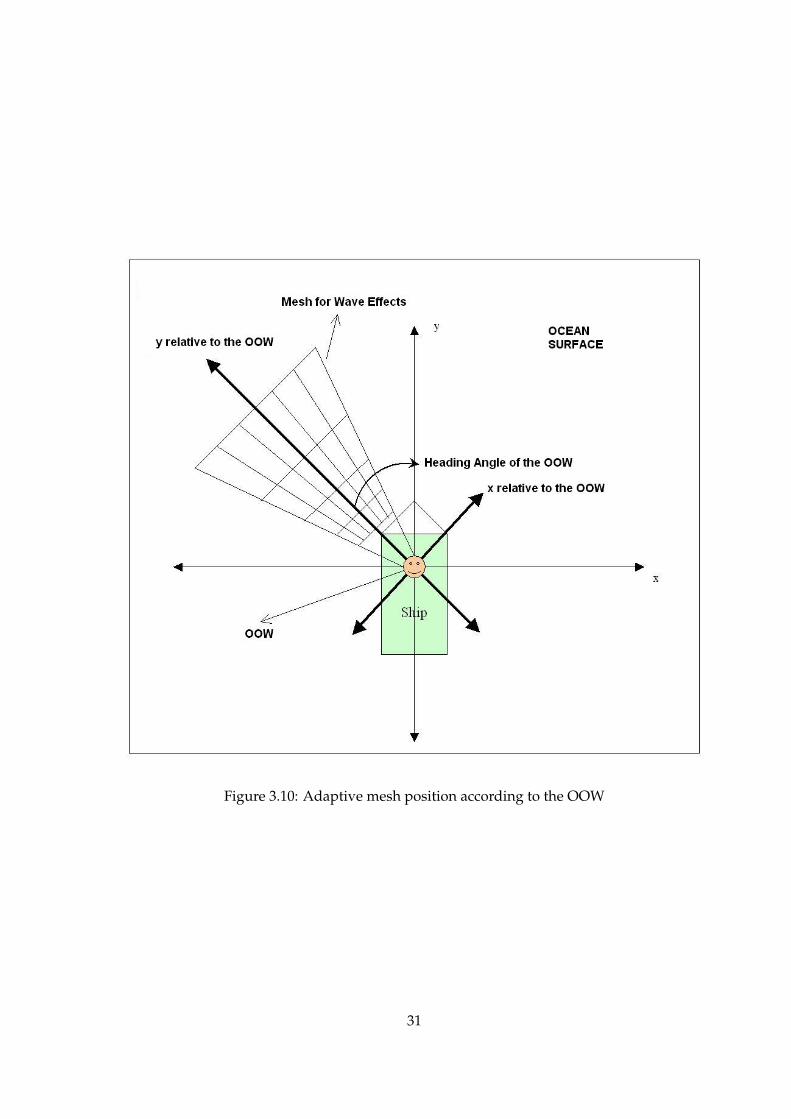
Figure 3.10: Adaptive mesh position according to the OOW

31

Figure 3.11: Appearance of the ship waves with normal mesh method

Figure 3.12: Appearance of the ship waves with incremental mesh method

32

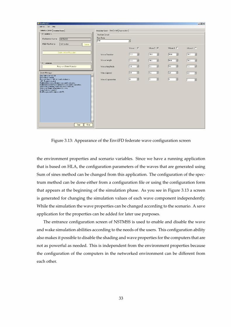
Figure 3.13: Appearance of the EnviFD federate wave configuration screen

the environment properties and scenario variables. Since we have a running application

that is based on HLA, the configuration parameters of the waves that are generated using

Sum of sines method can be changed from this application. The configuration of the spec-

trum method can be done either from a configuration file or using the configuration form

that appears at the beginning of the simulation phase. As you see in Figure 3.13 a screen

is generated for changing the simulation values of each wave component independently.

While the simulation the wave properties can be changed according to the scenario. A save

application for the properties can be added for later use purposes.

The entrance configuration screen of NSTMSS is used to enable and disable the wave

and wake simulation abilities according to the needs of the users. This configuration ability

also makes it possible to disable the shading and wave properties for the computers that are

not as powerful as needed. This is independent from the environment properties because

the configuration of the computers in the networked environment can be different from

each other.

33

3.4 Wave Shading Models

In virtual reality applications for a resembling view of natural phenomena, shadow mech-

anism has a big role. According to the light position and ambient light levels the shades

of objects must be created as in real life. Also to sea the moving objects and separate them

from other objects by perceiving their edges is possible with shading. For shading of the

object surfaces we need the angle between the surface normals and light source direction

vectors. So finding the surface normals is really important to simulate the shading of the

surface for better realism levels. Because our surface in the solution for wave generation

which will be explained in a more detailed way at chapter 5, is formed by combining a

number of quad shapes, the equation 3.3 can be used to find the updated position and

surface normals for each vertex is updated for finding shading levels. In this section two

methods will be studied and explained in a detailed way for finding the surface normals

to help the illumination of the waves. Before going into the detail of finding the normals,

the illumination method that is used in this thesis will be explained.

3.4.1 Illumination and Shading Process

In order to produce realistic scenes, we must simulate the appearance of surfaces under

various lighting conditions. Lighting effects are described with models that consider the

interaction of light sources with object surfaces. An illumination model is used to calculate

the intensity of the light that is reflected at a given point on a surface. A rendering method

uses intensity calculations from the illumination model to determine the light intensity at

all pixels in the image. In illumination models the light sources are thought to be point light

sources. These methods gives reasonably good approximations. Ambient illumination,

diffuse reflection and specular reflection forms the illumination model.

Ambient Illumination: It is assumed that there is a non directional light in the environ-

ment and it is called the background light. The amount of ambient light incident on each

object is constant for all surfaces and over all directions. This is a very simple model but

it is not very realistic. By default, OpenGL and Performer use this method. The reflected

intensity Iamb of any point on the surface is:

Iamp = KaIa

Ia is the ambient light intensity and

Ka ∈ [0, 1] - surface ambient reflectivity

34

Figure 3.14: Appearance of the ocean waves with ambient illumination

It is important to note that Ia and Ka are functions of color so we have IRa , IGa and IBa .

In Figure 3.14 only ambient illumination is used. Wave surface is realized to be a just a

flat surface.

Diffuse Reflection: A non-physical abstraction is made in diffuse reflection model. The

light source is thought to be a point light source. This model is also independent of viewer

position. The diffuse light intensity of a point changes according to the angle between the

normal vector and the light direction vector according to the point. The brightness at each

point is proportional to the cosine of this angle. As seen in Figure 3.15, the light reflected

from the point changes according to the angle between the normal vector and the light

vector. Diffuse reflection coefficient changes with the material properties of the surface.

Brightness is proportional to the cosine of θ because a surface is perpendicular to the light

direction is more illuminated than a surface at an oblique angle.

The reflected intensity Idiff of a point on the surface is:

35

Figure 3.15: Diffuse reflection according to the angles

Idiff = KdIpcos(θ) = KdIp(N • L)

Ip is the diffuse light intensity and

Kd ∈ [0, 1] - surface diffuse reflectivity

N is the surface normal

L is the light direction

It is important to note that L and N vectors must have a unitary length to make the

assumption of cos(θ) = (N • L). In Figure 3.16 waves are illuminated with ambient and

diffuse reflection models.

Specular Reflection: This illumination model helps to simulate the shiny and glossy

surfaces with highlights. Reflectance intensity of a point changes with reflected angle. In

Figure 3.17 the angle α between R and V effects the ratio of the surfaces specular reflection.

If α is 0◦ then the surface is assumed to be a perfect reflector. Glossy objects are not ideal

mirrors and reflect in the immediate vicinity of R. The Phong model which is used to find

the reflected specular intensity falls off as some power of cos(φ):

36

Figure 3.16: Appearance of the ocean waves with ambient and diffuse illumination

Ispec = KsIpcosn(φ) = KsIp(R • V )n

Ks is the surface specular reflectivity

R is the reflectance vector

V is the view vector

n is the specular reflection

parameter determining the deviation from ideal specular surface

After all these models the combined illumination model that is used in this thesis work

is :

I = Iamb + Idiff + Ispec

Since the intensity values are found for each vertex in the scene, the next job to do is

reflecting the new intensity values to each point in the screen. Different rendering methods

have been developed for this purpose like flat shading, gouraud shading and phong shad-

ing methods. Because it is really expensive to apply the illumination model at each surface

37

Figure 3.17: Specular reflection according to the angles

Figure 3.18: Appearance of the ocean waves with specular illumination

38

point these models are improved. Since the main purpose is not describing the illumina-

tion rendering methods, methods will not be given in detail. Three main methods can be

listed and summarized as follows:

Flat Shading: A single intensity is calculated for each surface polygon other than the

vertices. This method is really fast and simple but gives reasonably results if the following

assumptions are made:

• The object is a polyhedron

• Light source is far away from the surface so that N •L is constant over each polygon

• Viewing position is far away from the surface so that V • R is constant over each

polygon

An example simulating the flat shading model is given in Figure 3.19.

Gouraud Shading: Renders the polygon surface by linearly interpolating intensity val-

ues across the surface between vertices. This method is used in NSTMSS by using the

performer Gouraud Shading ability. The vertex intensity values of each element of the

wave mesh is found and they are interpolated for the other points in the wave mesh. In

[36] the gouraud shading method is explained in detail. Since gouraud shading has a good

performance in visualization and computation time it is acceptable for real-time systems.

Phong Shading: A more accurate method for rendering a polygon surface is to inter-

polate normal vectors, and then apply the illumination model to each surface point. This

method needs more computation time than the Gouraud method but gives better results

as you see in Figure 3.19. The steps in Phong method can be given as follows:

1. Determine the normal at each polygon vertex

2. Linearly interpolate the vertex normals over the surface polygon

3. Apply the illumination model along each scan line to calculate intensity of each sur-

face point

Before applying these illumination and rendering methods normal vector of each vertex

should be found. The methods for finding the normal vectors are explained in detail in next

two sub sections.

39

Figure 3.19: Polygon rendering methods

40

Table 3.3: Tangent, Normal and Binormal Vectors

Vector Notation Formula

Tangent T

T (t) =r

′(t)

|r′(t)|=

drdtdrdt

Normal N

N(t) =T

′(t)

|T ′(t)|

Binormal B

B(t) = T (t)×N(t)

3.4.2 Derivative Method

An explicit solution was presented in Mark Finch’s book [28]. To determine the rate of

change of the surface normals, the derivative can be taken in the x and y directions. By

taking the derivative two vectors which are called binormal and tangent are formed re-

spectively. The derivative in x direction is the tangent and the derivative in y direction is

the binormal vectors.

Before passing to the formulation, it is better to give some introduction to the tangent,

normal and binormal vectors. Let r(t) be a smooth vector-valued function in 2-space or

3-space. Then there are three important vectors which we define in Table 3.3. The three

vectors T, N and B form a triad of three mutually perpendicular vectors. So it can be said

that the normal vector is the cross product of tangent and binormal vectors. If we find each

of them then we will be able to have the normal vector of a point in the plain.

If it is assumed that the height field is oriented along the x-y grid then the binormal and

tangent vectors can be found as following:

Binormal(x, y) =(∂x

∂x,∂y

∂x,∂

∂x(f(x, y, t))

)simplifies to

Binormal(x, y) =(

1, 0,∂

∂x(f(x, y, t))

)

41

Tangent(x, y) =(∂x

∂y,∂y

∂y,∂

∂y(f(x, y, t))

)simplifies to

Tangent(x, y) =(

0, 1,∂

∂y(f(x, y, t))

)The cross product of the binormal and the tangent vectors is:

Normal(x, y) = Binormal(x, y)× Tangent(x, y)

Normal(x, y) =(− ∂

∂x(f(x, y, t)),− ∂

∂y(f(x, y, t)), 1

)Now, the derivatives of f(x,y,t) for each sine wave that are being composted for the final

position must be computed and sum up. To achieve that the derivative of f(x,y,t) with

respect to x and y are computed for each wave.

Differentiation with respect to x is:

∂

∂xf(x, y, t) =

12× steepness×Dir.X × frequency × amplitude×(sin(S) + 1

2

)steepness−1

× cos(S) where

S =Dir(x, y) • Pos(X,Y )× frequency + t× ϕ

Differentiation with respect to y is:

∂

∂xf(x, y, t) =

12× steepness×Dir.Y × frequency × amplitude×(sin(S) + 1

2

)steepness−1

× cos(S)

For the final surface normal we compute each component as follows and normalize the

result:

Normalfinal(x, y) =

(−

n∑i=1

∂

∂xf(x, y, t),−

n∑i=1

∂

∂yf(x, y, t), 1

)(3.8)

For each wave component (sine wave) the normals are found and summed. Before

using these normal valuew, the vector must be normalized. These normal values will be

used in the illumination process of the wave mesh.

In figure Figure 3.20 you can see an example simulation of shading with derivative

method. It is important to note that this method can just be used with the sum of sines

wave generation approach not with the spectrum analysis.

42

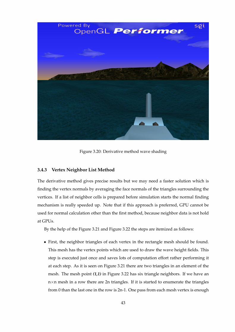
Figure 3.20: Derivative method wave shading

3.4.3 Vertex Neighbor List Method

The derivative method gives precise results but we may need a faster solution which is

finding the vertex normals by averaging the face normals of the triangles surrounding the

vertices. If a list of neighbor cells is prepared before simulation starts the normal finding

mechanism is really speeded up. Note that if this approach is preferred, GPU cannot be

used for normal calculation other than the first method, because neighbor data is not hold

at GPUs.

By the help of the Figure 3.21 and Figure 3.22 the steps are itemized as follows:

• First, the neighbor triangles of each vertex in the rectangle mesh should be found.

This mesh has the vertex points which are used to draw the wave height fields. This

step is executed just once and saves lots of computation effort rather performing it

at each step. As it is seen on Figure 3.21 there are two triangles in an element of the

mesh. The mesh point (1,1) in Figure 3.22 has six triangle neighbors. If we have an

n×n mesh in a row there are 2n triangles. If it is started to enumerate the triangles

from 0 than the last one in the row is 2n-1. One pass from each mesh vertex is enough

43

Figure 3.21: Normal Vectors and Quad Mesh Relation

Figure 3.22: Point and Neighbor Triangles Relation

44

to set the neighbor triangle positions.

• The second thing to do is calculating the normals of each triangle in the mesh at each

step. After the height field is updated and the points are set, normals are computed.

A triangle’s normal is equal to a normal of a point on it. Since we know the edge

vectors of each triangle, by taking the cross product of the two edges we will be able

to have the normal vector of the triangle. As it is seen on Figure 3.21 normals of

the points A and and D are the normal vectors of triangles 1 and 2 respectively. To

calculate the normals we need two vectors on the same surface at points A and D. For

instance at point A the vectors are−−→AB and

−→AC where the points are vectors in three

dimensional space. If a vector is needed from point B to A then subtracting the xB ,yB

and zB from xA,yA and zA respectively will give the vector−−→AB. The same is done for

point A and C to get the vector−→AC. If we cross product the vectors

−−→AB and

−→AC we

will get the normal vector of triangle 1. This step is repeated for each triangle on the

mesh.

• The third step is finding the normals of each vertex point in the mesh. For this step

the neighbor list array will be used. For each point on the mesh, the normals of all

neighbor triangles will be summed up and the average of them will be taken. For

example in Figure 3.22 for mesh point (1,1) it is easy to see that the neighbor triangles

are (0,1), (0,2), (0,3), (1,0), (1,1) and (1,2). The average of the normals of 6 of these

triangles will give the normal vector of mesh point (1,1).

• The last step in this algorithm is to decide the color levels of each vertex according to

the angle between the normal and the sun direction vector. Computing the shadow

levels according to the lights that are emitted and reflected is not within the scope of

this thesis.

In Figure 3.23 the vertex list method normal finding screen can be seen. Wave gener-

ation, mesh drawing and the other graphical properties like wave height, speed, frequen-

cies are the same. Only difference is the wave shading method other than the scene in

Figure 3.20.

3.5 Ship Wake Model

For resembling to natural phenomena more it is wanted that the ships leave a foamy path

on the sea that would be visible for a long time as it is in reality.

45

Figure 3.23: Vertex list method wave shading

Making visualization of wakes that ships leave behind as they travel can be done with

particle systems or with expending textures. In our situation as discussed before, real-time

is the main concern, texturing approach is more appropriate. But the modeling part is not

as easy as it is seen. The foamy part cannot be made as some moving polygons which are

attached to the ship and following it. It would also look strange because the foams must be

left behind and they should’t move forward or backward. Also, the foamy part of the sea

should expend by time and disappear in a while. It is ended up implementing the waves as

an expanding and semitransparent polygons of foamy components floating slightly above

the waving sea. As seen in Figure 3.24 each component of the polygon mesh is connected

continuously to previous components. To be more realistic the components are not left at

fixed intervals. If ship proceeds and passes a specified path length then the new polygon

is generated and added to the beginning of the wake polygon mesh. The initial size of a

component is defined by the width of a ship. To make the wave continuous at all times

new components are created inside the ship and stretched along the ships motion until

creating the next one. On the other hand also the path is not a straight path, since the

ship can turn left or right anytime. So the heading of each mesh vertex point must be

46

Figure 3.24: A ship from above, leaving wave components and a wave component.

47

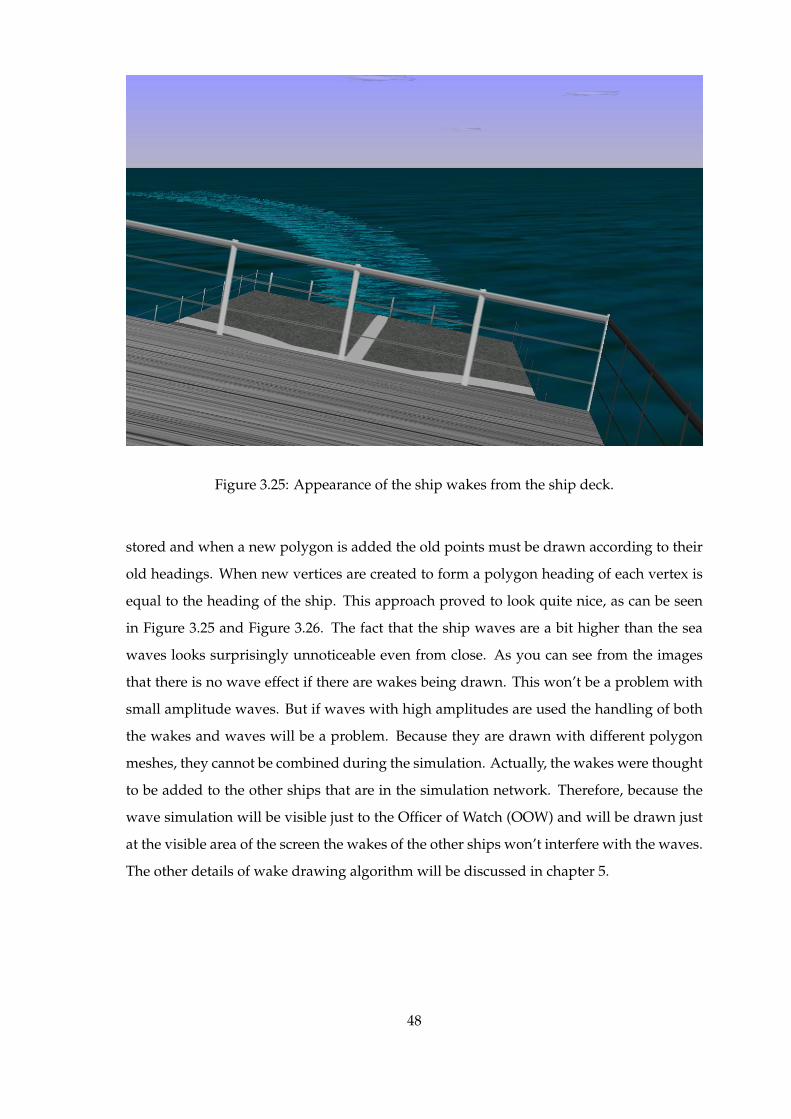
Figure 3.25: Appearance of the ship wakes from the ship deck.

stored and when a new polygon is added the old points must be drawn according to their

old headings. When new vertices are created to form a polygon heading of each vertex is

equal to the heading of the ship. This approach proved to look quite nice, as can be seen

in Figure 3.25 and Figure 3.26. The fact that the ship waves are a bit higher than the sea

waves looks surprisingly unnoticeable even from close. As you can see from the images

that there is no wave effect if there are wakes being drawn. This won’t be a problem with

small amplitude waves. But if waves with high amplitudes are used the handling of both

the wakes and waves will be a problem. Because they are drawn with different polygon

meshes, they cannot be combined during the simulation. Actually, the wakes were thought

to be added to the other ships that are in the simulation network. Therefore, because the

wave simulation will be visible just to the Officer of Watch (OOW) and will be drawn just

at the visible area of the screen the wakes of the other ships won’t interfere with the waves.

The other details of wake drawing algorithm will be discussed in chapter 5.

48

Figure 3.26: Appearance of the ship wakes from the stern of the ship.

3.6 Cloud Simulation

Making the sky look more realistic is another job in environment simulations. The clouds

are created from the polygons with cloud textures on them and these are randomly dis-

tributed. A possibility to make them drift along the wind was made easy to add but was

not implemented to the system and left as a future work. The cloud textures were found

from the internet and the images were filtered and edited and an alpha channel defining

their transparency was added. The regions of the images that does not contain any cloud

part in it were totally made transparent. That way, only the cloud pixels are visible and

the polygon does not appear as a rectangle but as the shape of the silhouette of the cloud.

This kind of clouds look good but raise another problem: If the flat clouds are placed at

different heights and parallel to the ground the clouds that are far, look really thin because

their view angle is small as depicted in Figure 3.27.

On the other hand in the sky the clouds can be seen as fat objects from which direc-

tion you look at them. In the visualization this was accomplished by rotating the clouds

perpendicular to the view relative their distance from the camera. The rotation is not very

49

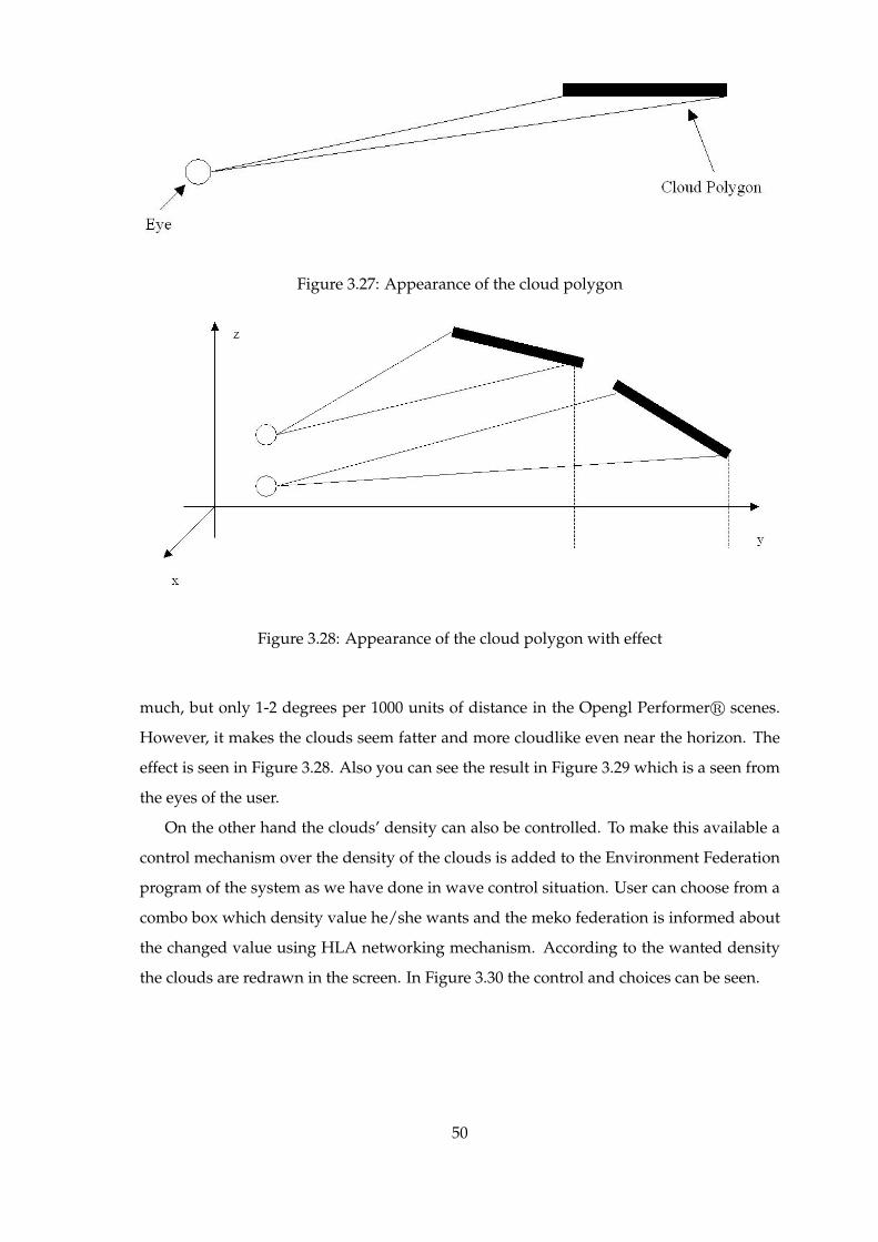
Figure 3.27: Appearance of the cloud polygon

Figure 3.28: Appearance of the cloud polygon with effect

much, but only 1-2 degrees per 1000 units of distance in the Opengl Performerr scenes.

However, it makes the clouds seem fatter and more cloudlike even near the horizon. The

effect is seen in Figure 3.28. Also you can see the result in Figure 3.29 which is a seen from

the eyes of the user.

On the other hand the clouds’ density can also be controlled. To make this available a

control mechanism over the density of the clouds is added to the Environment Federation

program of the system as we have done in wave control situation. User can choose from a

combo box which density value he/she wants and the meko federation is informed about

the changed value using HLA networking mechanism. According to the wanted density

the clouds are redrawn in the screen. In Figure 3.30 the control and choices can be seen.

50

Figure 3.29: A scene with clouds

Figure 3.30: Environment federation cloud density control

51

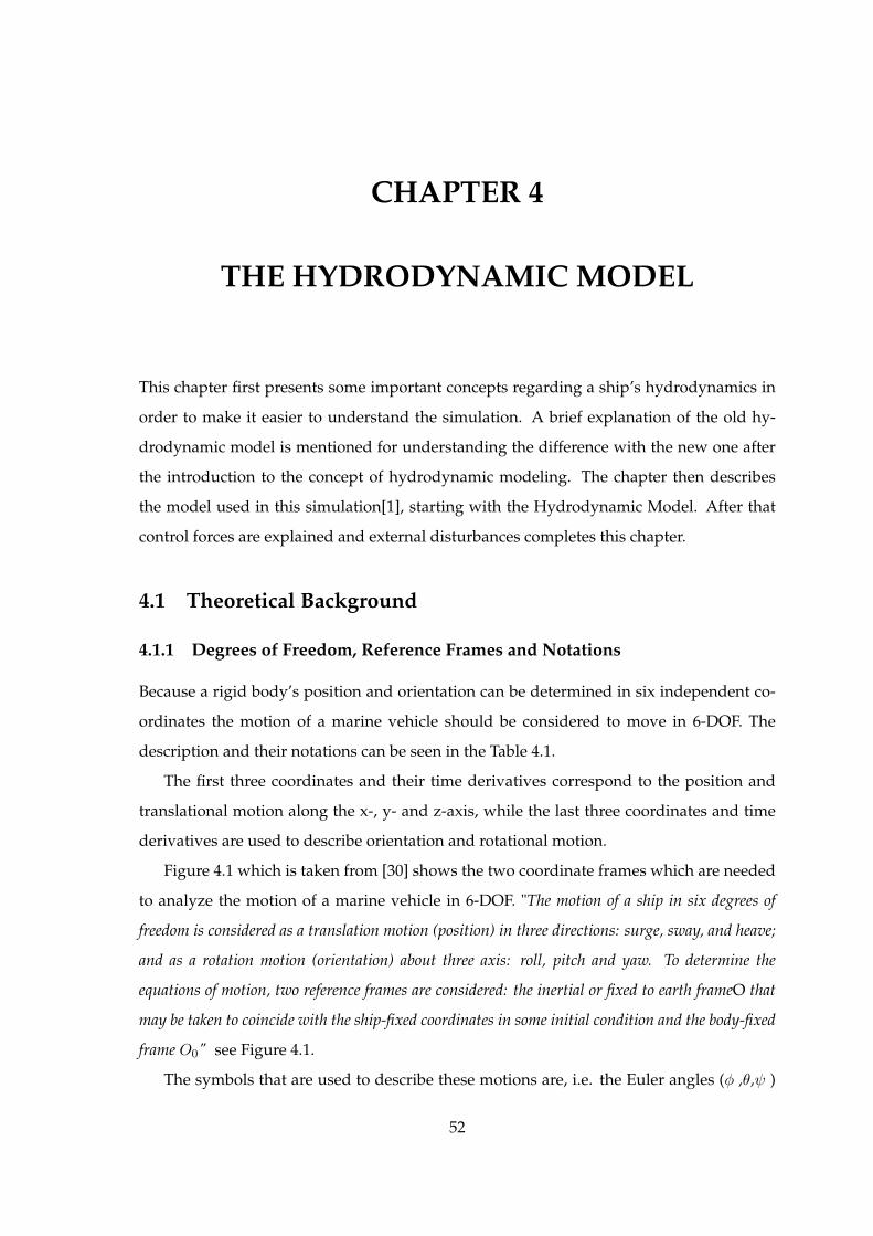
CHAPTER 4

THE HYDRODYNAMIC MODEL

This chapter first presents some important concepts regarding a ship’s hydrodynamics in

order to make it easier to understand the simulation. A brief explanation of the old hy-

drodynamic model is mentioned for understanding the difference with the new one after

the introduction to the concept of hydrodynamic modeling. The chapter then describes

the model used in this simulation[1], starting with the Hydrodynamic Model. After that

control forces are explained and external disturbances completes this chapter.

4.1 Theoretical Background

4.1.1 Degrees of Freedom, Reference Frames and Notations

Because a rigid body’s position and orientation can be determined in six independent co-

ordinates the motion of a marine vehicle should be considered to move in 6-DOF. The

description and their notations can be seen in the Table 4.1.

The first three coordinates and their time derivatives correspond to the position and

translational motion along the x-, y- and z-axis, while the last three coordinates and time

derivatives are used to describe orientation and rotational motion.

Figure 4.1 which is taken from [30] shows the two coordinate frames which are needed

to analyze the motion of a marine vehicle in 6-DOF. "The motion of a ship in six degrees of

freedom is considered as a translation motion (position) in three directions: surge, sway, and heave;

and as a rotation motion (orientation) about three axis: roll, pitch and yaw. To determine the

equations of motion, two reference frames are considered: the inertial or fixed to earth frameO that

may be taken to coincide with the ship-fixed coordinates in some initial condition and the body-fixed

frame O0" see Figure 4.1.

The symbols that are used to describe these motions are, i.e. the Euler angles (φ ,θ,ψ )

52

Table 4.1: DOF Description and Notations

DOF Description Forces and Linear and Positions and

index moments angular velocity Euler angles

1 Motions in the X u x

x-direction (surge)

2 Motions in the Y v y

y-direction (sway)

3 Motions in the Z w z

z-direction (heave)

4 Rotations in the K p φ

x-direction (roll)

5 Rotations in the M q θ

y-direction (pitch)

6 Rotations in the N r ψ

z-direction (yaw)

Figure 4.1: Reference Frames and Motion Variables

53

and the linear (u, v, w) and angular (p, q, r) velocity components, and the symbols denoting

the force (X, Y, Z) and moment (K, M, N) components. For the forces and velocities that

are used in naval applications, reference frames and motion variables in Figure 4.1 are the

most common ones. The names of the motions are given in parentheses next to axes for

translational motions and elliptic arrows for rotational ones. To the left of these names are

the related motion variables, which are body-fixed velocities, forces, and Euler angles, if

applicable. These quantities are given in a tabulated form in Table 4.1.

The general motion vectors of a naval vehicle in 6-DOF can be described by the follow-

ing vectors using the above notations:

v = [vT1 , vT2 ]T where v1 = [u, v, w]T and v2 = [p, q, r]T

τ = [τT1 , τT2 ]T where τ1 = [X,Y, Z]T and τ2 = [K,M,N ]T

η = [ηT1 , ηT2 ]T where η1 = [x, y, z]T and η2 = [φ, θ, ψ]T

It is important that in the following sections column matrix vectors will be represented

as bold and italic lower case letters where the bold and uppercase ones will represent the

square matrices. Translational quantities are also represented by the vectors which are sub-

scripted as "1" as you see in the above equations and rotational quantities are subscripted

as "2".

4.2 NSTMSS Old Hydrodynamic Model

Before discussing the old hydrodynamic model the forces acting on a marine vehicle should

be stated. These forces consist of external forces such as ocean current, prevailing winds

and wave action (or sea-state). Internal forces are those forces generated by the ship’s

propulsion machinery (e.g. propellers) and control surfaces (rudders). Internal and exter-

nal forces can be further classified into three categories controllable forces, semicontrollable

forces and uncontrollable forces.

Controllable Forces are the forces that are formed by the ship’s machinery that are con-

trolled by the bridge officer like rudders and propellers. Propellers of a ship generates a

thrust that moves the vehicle forward or backward while the rudder generates a compo-

nent of the thrust and creates a moment or torque about the center of gravity. The effect

of this torque causes the aft end of the ship to swing either to the port (left) or starboard

54

(right) side. It is these forces generated by the propeller/shaft combinations that must be

understood to steer the ship and present a good training mechanism for the ship simulator.

Semi-Controllable Forces are those forces that are generated by the surrounding area

that the ship is located in. These forces are usually present in narrow waterways where

thrust generated by the ship’s propellers and the wake resulting from the ship’s move-

ment through the water cause the immediate surroundings of the waterway (e.g. sides,

bottom...etc) to generate repelling forces which act against the ship.

Uncontrollable Forces are those caused by nature such as winds, currents and waves.

Conning officers have no control over these forces but must either compensate for them or

use them to their advantage.

In the NSTMSS project, controllable forces are modeled only; that is the effect of pro-

pellers and rudders, although the other two forces acting upon the ship, are important.

Because the NSTMSS project is thought to be just for formation maneuvering, and needed

to be accomplished in a short time period a basic hydro model that takes just the control-

lable forces into account is coded.

4.2.1 NSTMSS’s Simple Hydrodynamics Model

Because the focus of NSTMSS is not developing a complex mathematical model for a ma-

rine vehicle simulator the formulas of the used hydrodynamic model from NPSNET simu-

lator [37] [38] is not mentioned in a detailed way in NSTMSS Thesis. The references for the

algorithms and formulas are [39] and [40].

Before driving the formulas about the hydrodynamics model in NSTMSS because the

uncontrollable and semi-controllable forces are absent some behavioral characteristics are

decided to be eliminated according to the characteristics of the real environment. These

uncontrollable forces for example are high winds and large waves. The results of this

analysis determined that the ship would be operating in calm seas, which there are no

wave, current, and wind. Therefore, it is considered that heave and sway as negligible, as

well roll and pitch rates.

After these assumptions are made, it is concluded that the main focus will be on con-

trollable forces to provide ship−handling characteristics, such as ship’s turning diameter,

which is deeply affected by ship’s heading and speed that are the result of thrust, and

torque, since this is a simple simulator. Because another objective was to achieve an ade-

quate rendering performance complex arithmetic calculations were avoided by this simple

55

model.

The only DOFs in NSTMSS mathematical model are Surge and Yaw. The linear motion

of the ship, forward or backward, is generated by the thrust that is from the ship’s pro-

pellers. Thrust generated from propeller is obtained by multiplying the shaft speed by a

ship dependent constant. By the integration of acceleration, we obtain velocity of the ship.

The basic formula from [2] can be seen below.

F = m ∗ a

F = Totalthrust

Thrust = constant(newtons/RPM) ∗RPMs

V = V0 +∫ t

0(F/m)dt

When rudder is deflected by a certain amount of angle, the trust from the propeller

causes the rudder to generate a rudder torque. The Rudder Torque is figured out by multi-

plying the trust and sine of rudder deflection. When the rudder deflection is zero the aft of

the ship tends to swing right or left because of the turning of the shaft. Shaft Torque is de-

fined by multiplying the trust and lateral distance, which is the distance between shaft and

center of gravity. Total Torque is the sum of rudder and shaft torques. From total torque,

we find angular velocity and finally we find new heading by the sum of old heading and

angular velocity with respect to the time [2] and can be formulated as follows.

α = T/I

ω = ω0 +∫ t

0αdt

ψ = ψ0 +∫ t

0ωdt

4.3 Hydrodynamic Model

In the beginning of this thesis work, the 6-DOF model in [1] is planned to be used for

upgrading the hydrodynamic model. In literature there is no ship simulator model with

really 6-DOF mathematical model because of the lack of the hydrodynamics data. The

projects like [32] gives the details about six DOF but cannot accomplish to test their models

with real data to validate the correctness of the model. The 6-DOF models were needed to

56

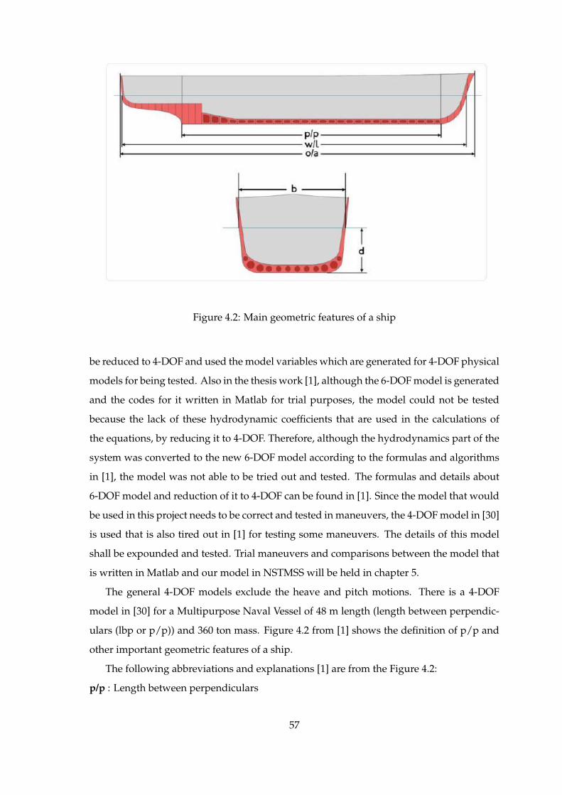
Figure 4.2: Main geometric features of a ship

be reduced to 4-DOF and used the model variables which are generated for 4-DOF physical

models for being tested. Also in the thesis work [1], although the 6-DOF model is generated

and the codes for it written in Matlab for trial purposes, the model could not be tested

because the lack of these hydrodynamic coefficients that are used in the calculations of

the equations, by reducing it to 4-DOF. Therefore, although the hydrodynamics part of the

system was converted to the new 6-DOF model according to the formulas and algorithms

in [1], the model was not able to be tried out and tested. The formulas and details about

6-DOF model and reduction of it to 4-DOF can be found in [1]. Since the model that would

be used in this project needs to be correct and tested in maneuvers, the 4-DOF model in [30]

is used that is also tired out in [1] for testing some maneuvers. The details of this model

shall be expounded and tested. Trial maneuvers and comparisons between the model that

is written in Matlab and our model in NSTMSS will be held in chapter 5.

The general 4-DOF models exclude the heave and pitch motions. There is a 4-DOF

model in [30] for a Multipurpose Naval Vessel of 48 m length (length between perpendic-

ulars (lbp or p/p)) and 360 ton mass. Figure 4.2 from [1] shows the definition of p/p and

other important geometric features of a ship.

The following abbreviations and explanations [1] are from the Figure 4.2:

p/p : Length between perpendiculars

57

w/l : Waterline length

o/a : Overall length

b : Breadth

d : Draft

4-DOF Hydrodynamic Model

The magnitudes describing the position and orientation of the ship are explained in sub-

section 4.1.1 in this chapter. It is important to note that the hydrodynamic model is first de-

fined in 6-DOF and will be reduced to 4-DOF. For starting to talk about the hydrodynamic

model position-orientation vector η with respect to the inertial frame must be defined first.

η , [x, y, z, φ, θ, ψ]T (4.1)

Linear-angular velocity vector ν with respect to the body-fixed frame is:

ν , [u, v, w, p, q, r]T (4.2)

Then, the position-orientation rate vector η is related to ν via:

η = J(η)ν (4.3)

J(η) is a transformation matrix that depends on the Euler angles (φ, θ, ψ). J(η)’s form

is as follows [22]:

J(η) =

J1(φ, θ, ψ) 03×3

03×3 J2(φ, θ, ψ)

(4.4)

J1 is :

J1(φ, θ, ψ) =

c(ψ)c(θ) −s(ψ)c(φ) + c(ψ)s(θ)s(φ) s(ψ)s(φ) + c(ψ)c(φ)s(θ)

s(ψ)c(θ) c(ψ)c(φ) + s(φ)s(θ)s(φ) −c(ψ)s(φ) + s(ψ)c(φ)s(θ)

−s(θ) c(θ)s(φ) c(θ)c(φ)

(4.5)

J2 is :

J2(φ, θ, ψ) =

1 s(φ)t(θ) c(φ)t(θ)

0 c(φ) s(φ)

0 s(φ)/c(θ) c(φ)/c(θ)

(4.6)

58

where c, s, and t means cos, sin and tan respectively.

The equations of motion of the vehicle according to the newtonian approach in the body

fixed frame can be given as:

MRB ν =τ(ν, ν, η)− CRB(ν)ν

η =J(η)ν

(4.7)

In equation 4.7MRB is the matrix mass and inertia due to rigid body dynamics,CRB(ν)ν

is the coriolis and centripetal forces and moments due to rigid body dynamics like MRB .

J(η) was given in equation 4.3.

The forces and moments vector τ is defined as follows:

τ = [X Y Z K M N]T (4.8)

The forces and moments vector can be generated with combination of different forces

in the nature.

τ = τhyd + τcs + τprop + τext (4.9)

The τhyd forces and moments are generated by the movement of the ship in the water.

The τcs are the forces and moments formed by the control surfaces like rudder and fins.

The τext are the forces and moments that are generated by the natural disturbances like

wind, waves and currents. The last τprop is generated by the propulsion system. In this

system because the heave and the pitch motions are neglected the following assumptions

can be made and the model is reduced to 4-DOF:

φ = p ψ = rcos(φ) (4.10)

The expanded form of equation 4.7 is as the following equation:

m 0 0 0

0 m −mzG mxG

0 −mzG Ixx 0

0 mxG 0 Izz

u

v

p

r

=

X

Y

K

M

+

m(vr + xGr

2 − Zgpr)

−mur

mzGur

−mxGur

, (4.11)

59

In the above equation:

• m is the mass of the ship,

• Ixx and Izz are the inertias about the x0 and z0 axis

• xG and zG are the coordinates of the center of gravity where CG = [xG, 0, zG].

The paper [30] mentions about all the forces acting on the ship except for the environ-

mental ones. The movement of the ship can be considered in two different situations, one

with incident waves and one without [30]. Because this model does not consider the natu-

ral forces the first approach, which is assuming the incident wave situation, is employed.

The hydrodynamic forces and moments originating from the first problem have dynamic

and static bases and can be studied by analyzing different originating effects. We will list

the effects here but the details can be found in [30]. The hydrodynamic forces and moments

arising from the first problem are listed as follows :

• Motion in an ideal fluid with no circulation: In this analysis, only the displacement is

considered, and it reveals the so-called added mass and inertia forces, moments and Munk

moment.

• Motion in an ideal fluid with circulation: In this analysis the shape of the hull is relevant.

• Motion in a viscous fluid: This analysis reveals the presence of hydrodynamic resistance.

• Gravitational and buoyancy forces: These are the restoring forces and moments that de-

pend on the Euler angles and act on the center of gravity CG and the center of buoyancy

CB.

Nonlinear function of the accelerations ν, velocities ν and Euler angles in η can be used

to model the forces and moments:

τhyd = f(ν, ν, η), (4.12)

and this model and forces can be written as a series expansion that is affine in the

parameters or coefficients. In equation 4.13 you can see the details for Yhyd force.

Yhyd ≈ Yvv + Yvvv2 + Yr|v|r|v|+ ... (4.13)

The constant coefficients in these equations are:

60

Yv =∂fY∂v

Yvv =∂2fY∂v2

Yr|v| =∂2fY∂r∂|v|

In technical report [30], after these details, also two examples, the model for the hydro-

dynamic forces of a container ship and the multi-role naval vessel model are given. These

models were obtained using the four degrees of freedom Roll Planar Motion Mechanism

(RPMM) facility at the Danish Maritime Institute. Since, in NSTMSS upgrade, the multi-

role naval vessel is used for improving the mathematical model, it will be explained here in

detail. Also the maneuver tests are done in [1] with using this 4-DOF method. Therefore,

the comparisons between the NSTMSS model and the matlab model will be available.

The surge equation is:

X = Xuu+X(u) + xvrvr + (1− t)T, (4.14)

where the resistance X(u) is:

X(u) = Xu|u|u|u| (4.15)

The sway equation is:

Y =Yvv + Yrr + Ypp

+ Y|u|v|u|v + Yurur + Yv|v|v|v|+ Yv|r|v|r|+ Yr|v|r|v|

+ Yφ|uv|φ|uv|+ Yφ|ur|φ|ur|+ Yφuuφu2

(4.16)

The roll equation is:

K =Kvv +Kpp

+K|u|v|u|v +Kurur +Kv|v|v|v|+Kv|r|v|r|+Kr|v|r|v|

+Kφ|uv|φ|uv|+Kφ|ur|φ|ur|+Kφuuφu2 +Ku|p|u|p|

+Kp|p|p|p|+Kpp+Kφφφφ3 − ρg∇Gz(φ)

(4.17)

The yaw equation is:

N =Nvv +Nrr

+N|u|v|u|v +N|u|r|u|r +Nr|r|r|r|+Nr|v|r|v|

+Nφ|uv|φ|uv|+Nφu|r|φu|r|+Kφu|u|φu|u|

(4.18)

In equation 4.17 the last term corresponds to the restoring roll moment, in which ∇

denotes the ship displacement, g the gravity constant, ρ the mass density of water, and

Gz(φ) is the buoyancy function for heel that can be approximated as :

61

Gz(φ) =(GM +

12BM tan2(φ)

)sin(φ) (4.19)

where GM is the metacentric height, and BM is the distance from the center of buoyancy

to the metacenter. The correct Gz curve is needed to get accurate results for large values of

heel.

In [1] three changes are made on the available added inertia coefficients. By making

these changes the model for the container ship that is proposed by Son and Nomoto in [22]

will be able to be solved by this 4-DOF model. The same ship model is used in the trials

for NSTMSS mathematical model.

Also the rudder and shaft models are taken from the container ship model of Son and

Nomoto. The shaft model is as follows :

n

nc=

1Tms+ 1

, Tm =

18.83, n < 20 rpm

5.65/n, n > 20 rpm(4.20)

where n and nc are the actual and commanded shaft speeds respectively and Tm is the time

constant for the shaft dynamics. The rudder model is:

δ

δc=

1s+ 1

(4.21)

where δ and δc are the current rudder angles and the commanded rudder angle, respec-

tively.

The detailed shaft and rudder models for 6-DOF can be found in [1].

62

CHAPTER 5

DEVELOPMENT ENVIRONMENT,

ALGORITHMS AND SIMULATION

RESULTS

Before giving details about the algorithms and results of the simulation trials the devel-

opment tools and environment are summarized. The section 5.2 gives the details of the

algorithms and shows them as pseudo codes for a better perception. In section 5.4 maneu-

ver trials for controlling the new hydrodynamic model is run and their results are com-

pared with the results of [1]. The performance test results of wave generation and shading

methods are the last parts of this chapter.

5.1 Development Environment

Microsoft Visual Studio 2005r was the development environment for NSTMSS. Also in

this thesis because the simulation base was coded in Visual Studio 2005 it is selected as the

development environment in the implementation process of the mathematical and graphi-

cal models. However, this tools has no tools for graphing, the data that is collected for test

procedures were analyzed at Microsoft Excel 2000r. Since the hydrodynamic model [1]

codes were written in Matlab 2007 r, for comparison tests it is also used.

This chapter will mainly focus on the content of the algorithm and how the individual

program components interact with each other. Since the algorithm development process is

independent of the tool/language used in the process, the issues regarding the integration

with the available software will be discussed in 5.2.

63

5.1.1 COTS (Commercial of-the-shelf)

In this section the tools that are used for graphical design and networking of the system will

be summarized. The NSTMSS system was designed to serve for distributed naval maneu-

vering simulations and designed on the HLA framework for networking. The graphical

subsystem is designed on OpenGL Performerr 3.2 which is a software from Silicon Graph-

ics. In the beginning phase of this project the graphical tool was planned to be changed to

Delta3D or DirectXr but this is left as a future work because of the time restrictions and

workload. The descriptions of the tools OpenGL Performer and RTI are taken from [2].

OpenGL Performer

OpenGL Performer provides a programming interface (with ANSI C and C++ bindings)

for creating real-time graphics applications and offers high-performance rendering in an

easy-to-use 3D graphics toolkit [41]. OpenGL Performer interfaces to OpenGLr graphics

library; these libraries form the foundation of a suite of tools and features for creating real-

time 3D graphics applications. NSTMSS uses OpenGL Performer v3.2 for MS Windows. A

visual database, also known as a scene, contains state information and geometry. A scene is

organized into a hierarchical structure, specifically as a directed-acyclic graph. The scene

hierarchy supplies definitions of how items in the database relate to one another. Addi-

tionally logical and spatial organization information of the database is also held within the

same hierarchy. The scene hierarchy is traversed by visiting the nodes in depth-first order

and operating on them. OpenGL Performer implements several types of database traver-

sals, including application, cull, delete, draw, and intersect. A logical hierarchy consists

of a set of objects grouped under a common parent according to the object type regardless

of position in the database whereas with a spatial hierarchy, the parent nodes that objects

are grouped under correspond to a particular position in the scene. The scenes in NSTMSS

processes are logical hierarchies. Geometry for the visual database may be created utiliz-

ing Performer’s high speed rendering library (libpr). A scene is rendered into a channel

or several channels, which are culled and drawn in the hardware graphics pipeline. A

view into the world is described by a channel. The remainder of the nodes in the database

includes moving and not moving coordinate systems, nodes containing geometry, anima-

tions, and nodes to switch between different sets of geometry. The actual geometry of the

scene, including light-points, is located at the leaf nodes. OpenGL Performer consists of

two main libraries, libpf and libpr, and four associated libraries, libpfdu, libpfdb, libpfui,

64

and libpfutil. Libpf is the main library, which handles multi-processed database traversal

and rendering and also contains libpr, which performs the optimized rendering, state con-

trol, and other functions fundamental to real-time graphics. Libpfdu is the library of scene

geometry building tools, which greatly facilitates the construction of database loaders and

converters. Libpfutil and Libpfui are utility functions and user interfaces respectively [41].

RTI (Real Time Infrastructure)

Run-Time Infrastructure (RTI) provides a specification of the functional interfaces between

federates and the RTI [42]. Interfaces are divided into six service groups. Each service spec-

ification includes: name and descriptive text, supplied arguments, returned arguments,

pre-conditions, post-conditions, exceptions, and related services. RTI Application Pro-

grammer Interfaces (APIs) are in CORBA IDL, C++, Ada95, and Java. NSTMSS software is

developed using the C++ API RTI software can be executed on a standalone workstation or

executed over an arbitrarily complex network. RtiExec (RTI Executive) is a global process.

Each federate communicates with RtiExec to initialize RTI components. The RtiExec’s pri-

mary purpose is to manage the creation and destruction of FedExecs. The RtiExec directs

joining federates to the appropriate federation execution. RtiExec also provides a naming

service for federation executives and ensures that each FedExec has a unique name. In

NSTMSS, DMSO RTI 1.3 NG-v3.2 version is used.

5.2 Algorithms

In this section the main algorithms that are developed to upgrade the NSTMSS simulation

system will be given in pseudo codes and explained.

5.2.1 Wave Generation Algorithms

Two of the wave generation algorithms which are mentioned in chapter 3 will be presented

in this section.

Sum of Sines Method

This method is basically the points in the space changing their z(height) values according

to some periodic signals whose properties can be changed. Below in Pseudo Code section

1 is the algorithm is given.

65

Pseudo Code 1 Algorithm for Sum of Sines wave generation method

input : position mesh, sine wave data(direction, amplitude,

wave length, wave speed, wave exponential)

output : new position mesh values

for each mesh point on x coordinate axis (i)

for each mesh point on y coordinate axis (j)

for each wave component (k)

1. frequency = (2 x PI) / WaveLength of the kth wave

2. DotProduct = Dot product of WaveDirection of kth

wave on xy-plane and the (i,j) point

on the mesh

3. phaseConst = time * WaveSpeed of the kth wave

* frequency;

4. S = DotProduct * frequency + phaseConst;

5. NormS = (sin(S) + 1) / 2;

6. Final Z = WaveAmplitude of the kth wave *

Norm S’s WaveExp of kth wave power;

7. If this is the 0th wave then the Final Z value will

be equalized to the z value of the mesh point (i,j).

if this is not the 0th wave then it will be summed to

the z value of the mesh point (i,j).

End If

end

end

end

66

As you can see this method is an easy to understand and fast to code in real time ocean

wave graphical programs. Besides, user can change all the properties in real time and also

the x,y values of the mesh points and he/she will get the same result with a steady wave

mesh. In the Implementation section of this chapter some screen shots can be seen of this

method with different mesh drawing methods. Since the performance is changed dramat-

ically by the number of mesh points and number of wave components, these performance

issues also will be discussed in detail.

JONSWAP Spectral Analysis Method

After the fast sum of sine method, the spectral analysis method with a long initialization

phase will be explained with a pseudo code section. In pseudo code 2 you will see the

initialization phase of the algorithm and like the first method the mesh points which are

stored in the initialization phase will be used during the simulation.

As you can see from the pseudo code 2 the storage and computational resources need

to be in good shape for a fast response of the simulator in the initialization phase. Even for

a small mesh and short time interval the performance results are not adequate.

The implementation codes can be found in Appendix section A.

5.2.2 Wave Mesh Surface Shading Algorithms

Two of the wave surface shading algorithms which are discussed in chapter 3 will be de-

tailed in this section.

Vertex List Method

The basic steps in this algorithm as stated in chapter 3 are vertex neighbor list generation,

finding normals of each triangle element of the mesh and averaging them for the vertex

normal vectors.

The initialization algorithm in Pseudo Code Part 4 is run in the initialization part of the

simulation before the main loop is started. So the computation afford for neighbor finding

is put out of the performance degrading processes. Besides, the normal finding part is run

in the wave drawing part based on the new mesh values that are calculated by the wave

generation algorithms. The computation complexity is n2 where the wave generation mesh

is n× n.

67

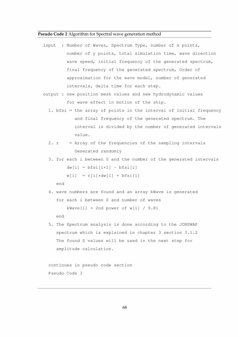
Pseudo Code 2 Algorithm for Spectral wave generation method

input : Number of Waves, Spectrum Type, number of x points,

number of y points, total simulation time, wave direction

wave speed, initial frequency of the generated spectrum,

final frequency of the generated spectrum, Order of

approximation for the wave model, number of generated

intervals, delta time for each step.

output : new position mesh values and new hydrodynamic values

for wave effect in motion of the ship.

1. bfsi = the array of points in the interval of initial frequency

and final frequency of the generated spectrum. The

interval is divided by the number of generated intervals

value.

2. r = Array of the frequencies of the sampling intervals

Generated randomly

3. for each i between 0 and the number of the generated intervals

dw[i] = bfsi[i+1] - bfsi[i]

w[i] = r[i]*dw[i] + bfsi[i]

end

4. wave numbers are found and an array kWave is generated

for each i between 0 and number of waves

kWave[i] = 2nd power of w[i] / 9.81

end

5. The Spectrum analysis is done according to the JONSWAP

spectrum which is explained in chapter 3 section 3.1.2

The found S values will be used in the next step for

amplitude calculation.

continues in pseudo code section

Pseudo Code 3

68

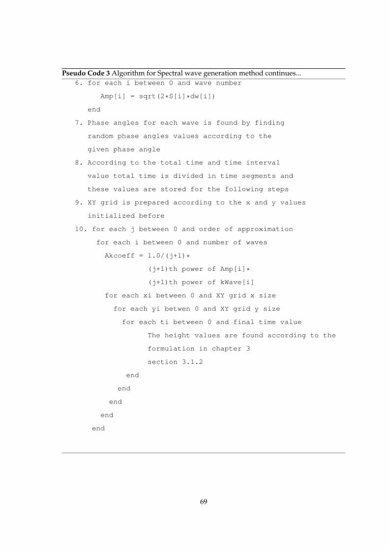
Pseudo Code 3 Algorithm for Spectral wave generation method continues...6. for each i between 0 and wave number

Amp[i] = sqrt(2*S[i]*dw[i])

end

7. Phase angles for each wave is found by finding

random phase angles values according to the

given phase angle

8. According to the total time and time interval

value total time is divided in time segments and

these values are stored for the following steps

9. XY grid is prepared according to the x and y values

initialized before

10. for each j between 0 and order of approximation

for each i between 0 and number of waves

Akcoeff = 1.0/(j+1)*

(j+1)th power of Amp[i]*

(j+1)th power of kWave[i]

for each xi between 0 and XY grid x size

for each yi betwen 0 and XY grid y size

for each ti between 0 and final time value

The height values are found according to the

formulation in chapter 3

section 3.1.2

end

end

end

end

end

69

Pseudo Code 4 Algorithm for Vertex Neighbor Initializationinput : Wave mesh size and vertex points.

output : Vertex Neighbor List.

for each i and j between 0 and the max numbers of x and y

if i == 0 and j == 0

vertexNeighbourList[i][j][0] = (0,0)

else if i == max number of x values AND j == max number of y values

vertexNeighbourList[i][j][0] is equal to (2*i-1, j-1)

else if i == 0 AND j == max number of y values

vertexNeighbourList[i][j][0] = (0, j-1)

vertexNeighbourList[i][j][1] = (1, j-1)

else if i == max number of x values AND j == 0

vertexNeighbourList[i][j][0] = (2*i-1, 0)

vertexNeighbourList[i][j][1] = (2*i-2, 0)

else if j == 0

vertexNeighbourList[i][j][0] = (i*2-2, 0)

vertexNeighbourList[i][j][1] = (i*2-1, 0)

vertexNeighbourList[i][j][2] = (i*2 , 0)

else if i == 0

vertexNeighbourList[i][j][0] = (0, j-1)

vertexNeighbourList[i][j][1] = (1, j-1)

vertexNeighbourList[i][j][2] = (0, j)

else if j == max number of y values

vertexNeighbourList[i][j][0] = (i*2-1, j-1)

vertexNeighbourList[i][j][1] = (i*2, j-1)

vertexNeighbourList[i][j][2] = (i*2+1, j-1)

else if i == max number of x value

vertexNeighbourList[i][j][0] = (2*i-1, j-1)

vertexNeighbourList[i][j][1] = (2*i-2, j)

vertexNeighbourList[i][j][2] = (2*i-1, j)

else if none of the controls are TRUE

vertexNeighbourList[i][j][0] to

vertexNeighbourList[i][j][6] are assigned to 6 neighbor values

70

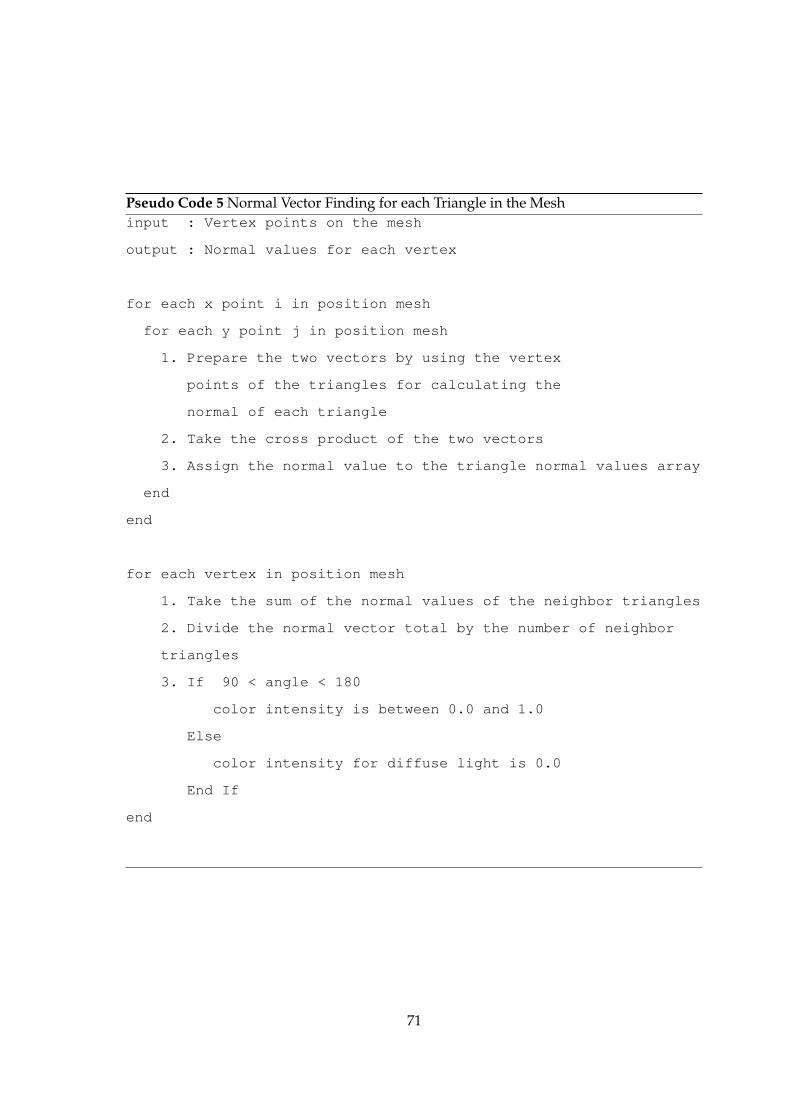
Pseudo Code 5 Normal Vector Finding for each Triangle in the Meshinput : Vertex points on the mesh

output : Normal values for each vertex

for each x point i in position mesh

for each y point j in position mesh

1. Prepare the two vectors by using the vertex

points of the triangles for calculating the

normal of each triangle

2. Take the cross product of the two vectors

3. Assign the normal value to the triangle normal values array

end

end

for each vertex in position mesh

1. Take the sum of the normal values of the neighbor triangles

2. Divide the normal vector total by the number of neighbor

triangles

3. If 90 < angle < 180

color intensity is between 0.0 and 1.0

Else

color intensity for diffuse light is 0.0

End If

end

71

Derivative Shading Method Algorithm

As mentioned in chapter 3 this method is explained as an extra method to get the normal

values of the wave mesh surface elements. Derivative method does not need any neigh-

bor data or initial values. For memory resource concerns this method is a better way to

compute the shading simulation. But the complexity grows as the number of waves gets

greater. The complexity as seen in the pseudo code 6 is n×n×k where the k is the number

of waves.

Pseudo Code 6 Derivative Normal Finding Method for each Vertex in the Meshinput : Vertex points on the mesh, and wave number

output : Normal values for each vertex

for each i between 0 and number of x values

for each j between 0 and number of y values

for each k between 0 and number of wave numbers

1. Derivative of the f(x,y,t), where f(x,y,t) is the function

that is used for finding the elevation in z, according to

x is calculated and assigned to derX.

2. Derivative of the f(x,y,t), where f(x,y,t) is the function

that is used for finding the elevation in z, according to

y is calculated and assigned to derY.

3. positionNorms[i][j].set(-derX, -derY, 1.0f)

end

end

5.2.3 Ship Wake Generation and Drawing Algorithm

As mentioned in chapter 3 the ship wakes are generated by expending polygon meshes

while the ship leaves behind on her path. The textures on wake polygons, as discussed

in cloud generation, are formed by enabling transparency for their background. This ap-

proach achieved drawing textures which does not have regular edges. By this method, the

72

cross section of the polygons to the sea textures are not recognizable by the user. In addition

to making the wake’s background fully transparent, it is wanted to make the wakes them-

selves a little bit transparent as well. This gave an effect of foamy ship wake simulation a

more realistic view. In pseudo code 7 you can see the algorithm details.

Pseudo Code 7 Wake Drawing Algorithminput : Each ship’s position in the performer scene

output : New wake polygon positions

for each ship on the ocean surface

1. Find the earth position of the new wake polygon’s

by using the relative lengths of the x and y positions

of the wake starting positions according to the moving

ship for future use.

2. The top two points of the quad is updated as the ship

changes her location and by this the top most polygon

is expended.

3. If ship has passed the position limit difference for

generating a new polygon than the 4 vertex points of the

polygon are calculated. Also the headings of each

polygon are saved for not losing their original orientation

according to the earth fixed frame.

4. After drawing the new polygon update the old polygons

according to the new one and by using their saved headings

and old positions they are drawn. Also expend them by

some ratio because of giving the effect of scattering foams.

5. Draw the wakes and if their life times are finished erase

them from the stack.

end

73

5.2.4 Wave Drawing Algorithm

The most important part in wave drawing part of this thesis is the adaptive scheme that

gives a much better performance and visual reality perception. This is because of the visual

wave drawing ability with a less number of mesh elements other than the normal mesh

drawing scheme. Besides the adaptive mesh characteristic also according to the heading of

the camera the mesh changes its position in the earth-fixed frame but it is not recognized by

the eyes of the users. While this effect is executed the direction of the waves are applied to

the newly generated mesh positions. This yields to an unchanged orientation of the waves

according to the old heading simulation results. Below is the algorithm for adaptive mesh

according to the changing heading. In appendix C you can see the code for creation phase

of this mesh which is the most important part.

In pseudo code 8 the adaptive mesh initialization and drawing is point out briefly.

5.2.5 4-DOF Hydrodynamic Model Algorithm

The algorithm is taken from the MATLAB code that is produced in [1]. This is the 4-DOF

hydrodynamic model that is created in [30]. The code snippets about the initialization and

the model process are in Appendix D. The hydrodynamic variables can be found in the

code samples.

5.3 Main Simulation Loop

In this section we will have a look at the main simulation run steps and gather all the

simulation steps that are talked about in this chapter, in chapter 3 and 4. The main steps

are shown in pseudo code 10.

5.4 Simulation Results

In this section first the maneuvering trials will be run to check the correctness of the model

code and they will be compared with the results in master thesis [1]. Performance tests will

be run according to the graphical and hydrodynamic models in the second sub section.

74

Pseudo Code 8 Adaptive Mesh Drawing Algorithminput : User’s current position and heading

Wave mesh points relative to the user starting

point.

output : New mesh points in the performer scene.

The mesh points are initialized relative to the user’s initial point

for drawing the mesh in the simulation phase according to the

changing position and heading of the viewer.

According to the adaptive scheme idea the quads are initialized to

have continuous level of detail (LOD) according to the distance from

the viewer. Quads have smaller edges then the ones that are far away

from the viewing point.

for each vertex on the mesh surface

1. Change the positions of the mesh points according

to the heading of the OOW. This is done by

calculating the earth-fixed vertex positions according

to the offsets of the mesh points which are

initialized in the starting phase of the simulation

executive considering the camera position.

2. Update the mesh points with the current wave drawing

algorithm.

end

75

Pseudo Code 9 4-DOF Hydrodynamic Model Algorithminput : current positional and translational state variables,

commanded shaft speed and rudder angle.

output: new positional and translational state variables.

1. Calculate the Hydrodynamic forces for Surge, Sway, Roll and Yaw

(X,Y,K,N) using the hydrodynamic coefficients. For calculation

details see the chapter 4 section 4.3.

2. Calculate the available thrust with respect to the propellers

according to the model explained in Hydrodynamic model section.

3. Add these thrust forces to the hydrodynamic forces matrix.

4. Rigid body inertia matrix and added inertia matrices are

calculated.The mass matrix is get by sum of the two matrices.

5. Initialize the Rigid body coriolis matrix.

6. According to the newton’s second law (F = m.a) find "a"

(acceleration values matrix) by calculating the inverse of the mass

matrix with the total force matrix.

7. After accelerations about all the axes are found the new position

and orientation values are found.

76

Pseudo Code 10 Main Simulation LoopBefore main loop execute the hydrodynamic model thread.

while the user does not exit the application

1. Process the HLA specific jobs and interchange the related data.

2. Draw all the ships on the screen

3. Time passed from the preceding time step (delta time) is given to

the main window for calculations of wave and wake simulations.

4. OOW’s position is set.

5. Performer’s callback functions are executed for drawing the

updated objects n the screen.

end

77

5.4.1 Maneuvering Trials

The maneuvering tests are the same with the ones at [1]. The frequently conducted ma-

neuvering tests are explained in [1] in detail. Here we will just check the results and cross

check their correctness. Some points are needed to be emphasized before passing to the

tests section. The delta time variable which is the time difference between two consecutive

simulation steps in our simulation software may vary but according to the measurements

the average value in the computer where the trials are tested between 0.05s and 0.06s. Also,

the matlab simulation code time step is chosen to be 0.06s since, in [1] the best timing for

Euler Integrator was found to be 0.06 seconds.

The test bench has a 1.83 GHz Intel Centrino processor , ATI Mobility Radeon X1400

graphics adapter and a Windows XP SP 2 operating system.

Turning Circle: The ship is given a 25◦ of rudder (this is the maximum allowed) to the port

side and full ahead. Then the ship is observed in heading, planar motion, roll angle and

velocity values. The MATLAB 4-DOF model is also run and the graphs are compared with

each other. There is a little change in roll motion and because of that the planar motion

is a little bit late in MATLAB mode. This is because of the difference in precision control

between MATLAB and C++ Visual Studio 2005. It can be observed from Figure 5.1 to

Figure 5.10 the results are really similar.

In Figure 5.1 and Figure 5.2 the roll angles are observed and with the rudder and thrust

commands applied, both models are responding with the same roll angles at the same time.

Stopping Trial: The ship is given a full ahead surge command and after 100 seconds, the

command is reversed until the ship stops completely. The surge velocity graph below is

the most important result of this test. From Figure 5.11 to Figure 5.14 can be observed to

see the results of both the c++ code and the matlab code are the same. The time steps are

also proven to be precise for euler integration in solving the model.

Pull-Out Maneuver: The rudder is held at its zero position until the ship gains a steady

surge velocity. After 70 seconds of a straight line cruise, which is necessary for this purpose,

the rudder is given a 20 degree starboard command, and this is held until the ship attains

a steady state turn rate. After 300 seconds the rudder is taken back to its 0 position and the

motion of the ship is observed. The data that is collected from both the matlab model and

the c++ model can be observed in figures between Figure 5.15 and Figure 5.20.

78

Figure 5.1: NSTMSS turning circle roll angle change

Figure 5.2: Matlab turning circle roll angle change

79

Figure 5.3: NSTMSS turning circle planar motion change

80

Figure 5.4: Matlab turning circle planar motion change

Figure 5.5: NSTMSS turning circle heading angle change

81

Figure 5.6: Matlab turning circle heading angle change

Figure 5.7: NSTMSS turning circle velocity change

82

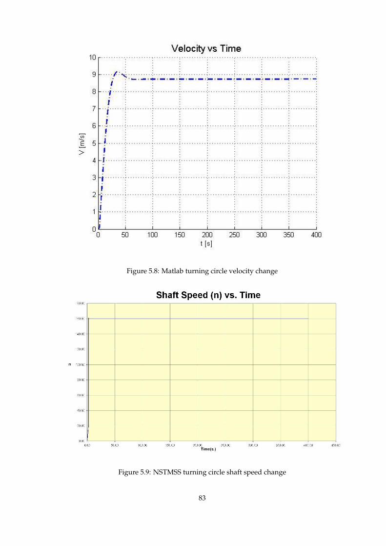
Figure 5.8: Matlab turning circle velocity change

Figure 5.9: NSTMSS turning circle shaft speed change

83

Figure 5.10: Matlab turning circle shaft speed change

Figure 5.11: NSTMSS stopping shaft speed change

84

Figure 5.12: Matlab stopping shaft speed change

Figure 5.13: NSTMSS stopping velocity change

85

Figure 5.14: Matlab stopping velocity change

Figure 5.15: NSTMSS pull out heading change

86

Figure 5.16: Matlab pull out heading change

87

Figure 5.17: NSTMSS pull out planar change

Direct Spiral Maneuver:This maneuver is like pull out one, however the rudder is taken

back to mid-ship position incrementally. 20 degrees of rudder angle is recovered to zero

with pauses at 20-10-5-3-2-1-0 degrees. At each increment 100 periods are allowed to pass

to reach incremental turn rates. The planar trajectory, heading angle and roll angle graphs

are given from Figure 5.21 through Figure 5.26, respectively.

When the results for all maneuver trials are observed from both of the c++ and matlab

codes it can be stated that the c++ hydrodynamic code is proven to be exactly the same

with the Matlab model.

5.4.2 Performance Tests

As mentioned in chapter 1 the main performance issues in this system and the systems like

this are the real-time and graphical performance. Since the aim of these kind of systems is

to give the user, the perception of real life by simulation there must not be any hesitation

in the view or in the real-time calculation parts. The performance trials of the system are

mainly gathered around these issues.

88

Figure 5.18: Matlab pull out planar change

Figure 5.19: NSTMSS pull out roll change

89

Figure 5.20: Matlab pull out roll change

Figure 5.21: NSTMSS spiral maneuver roll change

90

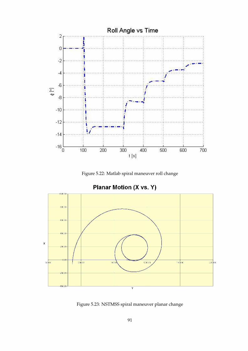
Figure 5.22: Matlab spiral maneuver roll change

Figure 5.23: NSTMSS spiral maneuver planar change

91

Figure 5.24: Matlab spiral maneuver planar change

Figure 5.25: NSTMSS spiral maneuver velocity change

92

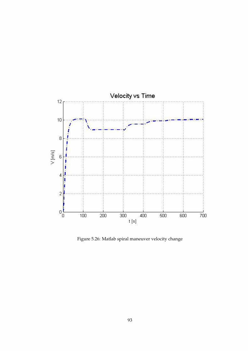
Figure 5.26: Matlab spiral maneuver velocity change

93

Table 5.1: Tests of Wave Generation MethodsSpectrum Analysis Sum of Sines Sum of Sines

with 10 waves with 2 waves with 4 waves

30×30 mesh grid 16.30 FPS 16.10 FPS 15.90 FPS

40×40 mesh grid 15.40 FPS 15.00 FPS 14.70 FPS

50×50 mesh grid 15.30 FPS 14.00 FPS 13.80 FPS

60×60 mesh grid 13.90 FPS 13.60 FPS 13.00 FPS

70×70 mesh grid 12.20 FPS 12.45 FPS 12.00 FPS

90×90 mesh grid 11.00 FPS 10.90 FPS 10.60 FPS

Wave Generation Method Trials

The two methods that were developed are sum of sines and the JONSWAP spectrum analy-

sis method. The main difference between the two methods is that the spectrum analysis

method relies on the real data that is collected for decades but the first one is generated in

real time according to the sine functions. However we can get the same simulation scenes

by the first method if we have the data about the wave characteristics. The other difference

is the real time performance. Since the spectrum analysis wave data is generated before

the scene is started more wave components can be simulated without any performance

decrease. But in the first method if the number of waves are more than 4 the performance

is effected dramatically. On the other hand, the pause before the simulation for the genera-

tion of waves and the unchangeable character of the second spectrum method makes it less

desirable than the sum of sines method. The test results that are collected by performing

the control of FPS (Frames Per Second) can be seen in the Table 5.1. These executions have

also wave effects and that factor decreases the frame count also. The scene has a FPS of

18.7 without any wave effect.

As you see in Table 5.1 also the wave mesh size gets bigger, spectrum analysis methods

shows similar performance. The little change is originated from the vertex shading algo-

94

rithms. This is because the mesh height values is pre-calculated. But, this is not the same

with the sum of sines method because of the increasing number of calculation in real time.

Although the computation time does not change in spectrum analysis method, with the

increasing number of wave mesh elements the storage for holding the calculated values

expands. If you have a storage concern this method won’t work for large meshes. It is

important to note that the performance of the system will also be affected by the computer

configuration of the test bench. The second important point in these tests is that the per-

former is not set for any frame duration in the simulation initialization face. The tests are

done with the Performer’s best frame duration available calculation mode.

Wave Shading Method Trials

The two shading methods don’t have much difference in performance between each other.

But it is necessary to check the performance tests to decide which one to use. The same

situation that is the computer configuration like in wave generation tests, is seen here. For

this test, the mesh size is taken to be 40×40, sum of sines wave and the adaptive mesh

technics are employed for the scene. The Vertex List Shading Method has given 14.00 FPS

where the Derivative Method had a result of 15.50 FPS which is a better result. The same test

is also done without any shading and the result with the derivative normal finding method

was 15.00 FPS. One last test is also run without the adaptive mesh heading effect technic

and it was obvious that the OOW heading effect did not really affect the performance. The

FPS value was 16 FPS and it was similar to the the ones with heading effect simulation

scenes. As far as we had seen the performance tests had given acceptable results and the

scenes were drawn in an adequate screen frame frequencies in the perception ranges of a

human’s eye.

95

CHAPTER 6

CONCLUSIONS AND FUTURE

DIRECTIONS

In this chapter an overall summary of the topics that are discussed is explained briefly and

the conclusion of the thesis work is given in section 6.2. The last section is giving details

about the future work ideas.

6.1 Summary of the Thesis

The simulators that were introduced in chapter 1 have an important role in training and

experience life of young officers. Other than the million dollar motion based simulators,

the networked pc simulators that are easy to transport and install also have a big role in the

life of daily education. Since there is a need in this field, naval and flight simulators need

to catch up with the real-time simulation issues and visualization realism levels. NSTMSS

is one of these simulators that is practical to use, inexpensive and expendable in different

ways.

This Master’s Thesis researched the current trends and technologies about ship hydro-

dynamics and ocean simulation issues. The properties of other up-to-date simulators were

reviewed and studied. The reader was introduced to a variety of important and interesting

projects and products, from past to current ones. Emphasis of the research was placed on

areas of real-time visualization and realism levels, which were the two major areas in the

systems like NSTMSS.

First of all two kinds of wave generation methods are explained and integration of

them to the NSTMSS system is studied. The comparisons and tests of each approach are

examined in a detailed way. The algorithms and codes are explained in chapter 5 and

Appendix A respectively. Since the visualization of the ocean waves is an important issue

96

the shading and drawing models of wave generation techniques are clarified. In chapter

3 the shading models which are neighbor vertex list method and the derivative method are

explained. The adaptive mesh method for drawing the mesh grid is also discussed in

chapter 3.

The details of the new four degrees of freedom hydrodynamic model is explained in

chapter 4. After a little introduction to the concepts of mathematical models, the new

physical model is put forward by introducing the equations of motions, and explaining the

forces that act on the ship in detail.

In chapter 5 the details for each algorithm that is developed in thesis is stated. Before

that the development environment and used technologies are summarized. The most im-

portant part that would clarify the correctness of the model that is implemented, is the

maneuver trials and the performance tests. These sections ends this chapter.

6.2 Conclusion

In the hydrodynamics part of this thesis work some computational improvements accord-

ing to [1] are made. These improvements are also reflected to the implementation of

NSTMSS hydrodynamic model. The improvements are transformation matrix construc-

tion, hydrodynamic force calculation, wave force computation, etc. In the simulation loop

of the model to increase the computation performance, the variables that needs to be cal-

culated once are took into account in the initialization face. Also in the main cycle the

reusable variables are calculated once and used where needed. These are the trigonometric

functions of the euler angles that are used in transformation matrices. These improvements

increased the real time performance.

The second goal was to improve the visual abilities. For this purpose, ocean wave mod-

eling and ship wake simulations are integrated to the NSTMSS system. While generating

the code for graphical design the old code was commented and indentation was checked.

Different ways to design the algorithms for ocean waves are investigated and compared

with each other to find the one with best performance. The Sum of Sines method is em-

ployed for this purpose and the shading of the wave mesh was done within the same wave

simulation function by derivative method which gives a better performance over vertex

neighbor list normal finding method. The dynamic change of the position and heading of

the user also draw us to find a method to change the position and orientation of the wave

mesh. The adaptive mesh technique was chosen for this manner. The main goals that are

97

accomplished can be listed as follows:

• Upgrading of the hydrodynamic model of the NSTMSS from a basic motion model

to a 4-DOF model is accomplished.

• The design and implementation of graphical ocean wave models are accomplished.

• Different surface shading models for a realistic scene are studied.

• Dynamically changeable simulation scene for wave drawing is studied and inte-

grated to NSTMSS.

• A new ship wake simulation approach is designed and implemented.

It is important to note that, mainly the adaptive wave mesh drawing method has in-

creased the performance and visualization of wave effects. With adaptive technique, which

has a same number of quads with a normal mesh, simulation ability increases by using the

same computational power and the FPS values of the Performer scenes do not decrease

and are within the range of the acceptable values. Rather drawing the wave simulation

for all the ocean surface, visualizing the wave mesh just in the visible scene of the viewer

according to the FOV angle, has also increased the performance considerably.

6.3 Future Work

One line of future work for the NSTMSS system can mostly be increasing the realism level

by giving importance to the graphical user interface and hydrodynamics model. The hy-

drodynamic model should have natural disturbance forces which are waves, wind and

ocean currents. These will give a more realistic approach to the training. If the user has

a visual about a natural event (for example waves) it would be better to give user the ef-

fects of the natural disturbances as the hydrodynamic forces which shows their effects as

motion. This will lead to a better perception of natural phenomena.

One of the most important future work is to the images were filtered and edited and an

alpha channel defining their transparency. The data set is important for true hydrodynamic

model solutions. After the related data is found the maneuver tests should be run again to

validate the mode.

The control of the ocean wave parameters should be added to the environment fed-

erate for immediate property changes in visual environment. One of the most important

98

example for this is wave property changes like wind speed, wave direction and wave char-

acteristic properties.

A future work for graphical improvements of the system can be implementing the mo-

tion and drifting of the clouds with the weather effects. According to the speed of the wind

and natural disturbances the cloud density and their position can be changed.

In the wave generation methods the spectrum analysis method properties cannot be

changed during the simulation. Since the wave model is based upon the data that is gener-

ated before the simulation steps, the change of wind velocity and direction is not possible

during the simulation. Dynamic updating of the wind velocity and direction may be inte-

grated into the system by utilizing the environment federate of NSTMSS. This way a more

realistic wave simulation can be achieved.

99

APPENDIX A

SAMPLE CODES FOR WAVE GENERATION

A.1 Sum of Sines Method Code

for( int i = 0; i < numofwavequads + 1 ; i++){

for ( int j = 0; j < numofwavequads + 1 ; j++ ){

for ( int k = 0 ; k < numofwaves ; k++ ){

freq = 2.0f * (double)PI / waveLength[k];dotResult = waveDirection[k].vec[0]*

positionMesh[i][j].vec[0] +waveDirection[k].vec[1]*positionMesh[i][j].vec[1];

dotResult *= freq;phaseConst = t * waveSpeed[k] * freq;final = dotResult + phaseConst;S = final; // for later usefinal = (sin(final) + 1.0f) / 2.0f;final = waveAmplitude[k] * pow(final, waveExp[k]);if ( k == 0 ){

positionMesh[i][j].vec[2] = final;}else{

positionMesh[i][j].vec[2] += final;}

}}

}

100

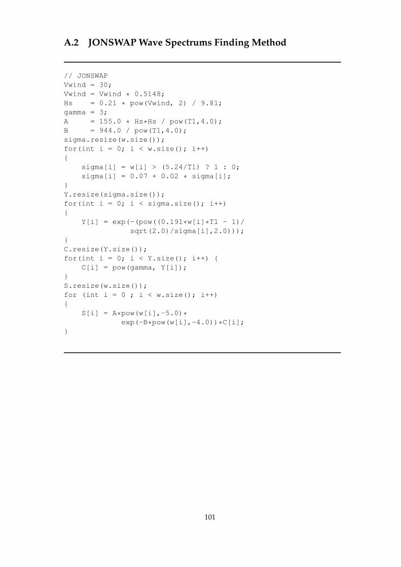
A.2 JONSWAP Wave Spectrums Finding Method

// JONSWAPVwind = 30;Vwind = Vwind * 0.5148;Hs = 0.21 * pow(Vwind, 2) / 9.81;gamma = 3;A = 155.0 * Hs*Hs / pow(T1,4.0);B = 944.0 / pow(T1,4.0);sigma.resize(w.size());for(int i = 0; i < w.size(); i++){

sigma[i] = w[i] > (5.24/T1) ? 1 : 0;sigma[i] = 0.07 + 0.02 * sigma[i];

}Y.resize(sigma.size());for(int i = 0; i < sigma.size(); i++){

Y[i] = exp(-(pow((0.191*w[i]*T1 - 1)/sqrt(2.0)/sigma[i],2.0)));

}C.resize(Y.size());for(int i = 0; i < Y.size(); i++) {

C[i] = pow(gamma, Y[i]);}S.resize(w.size());for (int i = 0 ; i < w.size(); i++){

S[i] = A*pow(w[i],-5.0)*exp(-B*pow(w[i],-4.0))*C[i];

}

101

APPENDIX B

SAMPLE CODES FOR WAVE SHADING

B.1 Derivative Method

This code is a part of the Sum of Sines wave generation code. It is in the same loop with it.

if ( SHADING_METHOD == DERIVATIVE_METHOD ) {derX = (1.0f/2.0f) * waveExp[k] * waveDirection[k].vec[0]

* freq * waveAmplitude[k] *pow((sin(S) + 1.0f) / 2.0f, waveExp[k] - 1.0f) * cos(S);

derY = (1.0f/2.0f) * waveExp[k] * waveDirection[k].vec[1]

* freq * waveAmplitude[k] *pow((sin(S) + 1.0f) / 2.0f, waveExp[k] - 1.0f) * cos(S);

if ( k == 0 ){

positionNorms[i][j].set(-derX, -derY, 1.0f);}else{

positionNorms[i][j].set(positionNorms[i][j].vec[0] - derX,positionNorms[i][j].vec[1] - derY,1.0f);

}}

102

APPENDIX C

SAMPLE CODES FOR WAVE MESH

GENERATION

C.1 Adaptive Mesh Method

int limit = numofwavequads / 2;int signx = 1.0f;

for ( int j = 0; j <= numofwavequads; j++ ){

for ( int i = limit, signx = 1; i >= -limit; i-- ){

if ( i == 0 ){

signx = -1;}

if ( j==0 ){

if ( OOW_HEADING_EFFECT == EFFECT_ON ){

positionMesh[limit-i][j].set( -i * 2.0f ,10.0f,2.0f );

}else{

// These positions are are not according to the OOWpositionMesh[limit-i][j].set(

i * 2.5f,parent->oow->position->xyz[1] - 10.0f,2.0f );

}}

103

else{

if ( OOW_HEADING_EFFECT == EFFECT_ON ){

newX = positionMesh[limit-i][j-1].vec[0] -tan(DEG_TO_RAD*i*plusAngle)*j*5.0f;

positionMesh[limit-i][j].set(newX,positionMesh[limit-i][j-1].vec[1] + j*5.0f,2.0f);

}else{

newX = positionMesh[limit-i][j-1].vec[0] +tan(DEG_TO_RAD*i*plusAngle)*j*5.0f;

positionMesh[limit-i][j].set(newX,positionMesh[limit-i][j-1].vec[1] - j*5.0f,2.0f);

}}

}}

104

APPENDIX D

SAMPLE CODES FOR 4-DOF

HYDRODYNAMIC MODEL

First section is initialization of the hydrodynamic variables of the container ship from

the model of Son and Nomoto[22]

// Hydrodynamic derivatives// Force coefficientsdouble Xuu = -1960;double Yuv = -11800;double Kuv = 9260;double Nuv = -92000;double Xvr = 0.33*m;double Yur = 131000;double Kur = -102000;double Nur = -4.71e6;double Yvv = -3700;double Kvv = 29300;double Nvv = 0.0;double Yrr = 0.0;double Krr = 0.0;double Nrr = -202e6;double Yvr = -0.794e6;double Kvr = 0.621e6;double Nvr = 0.0;double Yrv = -0.182e6;double Krv = 0.142e6;double Nrv = -15.6e6;double Yphiuv = 10800;double Kphiuv = -8400;double Nphiuv = -0.214e6;double Yphiur = 0.251e6;double Kphiur = -0.196e6;double Nphiur = -4.98e6;double Yphiuu = -74;

105

double Kphiuu = -1180;double Nphiuu = -8000;double Yup = 0.0;double Kup = -15500;double Nup = 0.0;double Ypp = 0.0;double Kpp = -0.416e6;double Npp = 0.0;double Yp = 0.0;double Kp = -0.5e6;double Np = 0.0;double Yphi = 0.0;double Kphi3 = -0.776*rho*g*nabla;double Yphiphiphi = 0.0;double Nphi3 = 0.0;double Nphi = 0.0;double Ydeltauu = 2*3.5044e3;

// Added inertia termsdouble Xu_d = -17400;double Yv_d = -393000;double Kv_d = 296000;double Nv_d = 538000;double Yr_d = -1.4e6;double Kr_d = 0.0;double Nr_d = -38.7e6;double Yp_d = 0.296e6;double Kp_d = -0.774e6;double Np_d = 0.0;

This second code snippet is about the main simulation loop and where the thread is

started can be seen:

//Thread is started herethis->ship->engine->startHydroModel();

while (this->FederateState!=MekoFd::FederateStates::ExitApplication){

this->ship->radar->tss->rtiAmb->update();CrtiAmb::tick();

// PRE-FRAME// All latency critical processing should be done here.dt = getTimeStep();// measure the simulation time stepFrameRate = 1/dt; // Calculate the current frame rate

//this->ship->tss->deadReckonGhosts();

106

this->window->setShipDCS(this->ship->radar->tss->TrackList);

// Set dt for ship wake drawingthis->window->setdt(dt);

// Position OOWthis->oow->setPosture();

// Go to sleep until next frame time.pfSync();

// Set Main Camera Viewthis->window->mwChan->setView(this->oow->position->xyz,this->oow->position->hpr);

// FRAMEpfFrame();

//POST-FRAME// DirectInput Processingthis->ui->processMouse();this->ui->processKeyboard();

// process application eventsApplication::DoEvents ();

// Write Frame Per Second//Console::WriteLine("Frame Rate="+1/dt);

};//End of while

The last code part is the main hydrodynamic model execution part:

double nc,deltac;static int writeCount = 0;int signdeltadot;double deltadot;int signdeltac;int signnc;double Tm;

// states : Augmented state variable vector for the 4-DOF modeldouble u = states.u;double v = states.v;double p = states.p;

107

double r = states.r;double x = states.x;double y = states.y;double phi = states.phi;double psi = states.psi;double delta = states.delta;double n = states.n;

// Commanded shaft speed [rpm]nc = orderedRPMStbd;

// Commanded shaft speed [rpm]deltac = rudderAngle;

// Rudder angle limit [degree]double deltamax = 45;// Rudder rate limit [degree/s]double deltadotmax = 20;

// Degree -> radian conversionsdeltamax = DEG_TO_RAD * deltamax;deltadotmax = DEG_TO_RAD * deltadotmax;deltac = DEG_TO_RAD * deltac;

// Calculation of the hydrodynamic forcesdouble Xh = Xuu*u*abs(u) + Xvr*v*r;

double Yh = Yuv*abs(u)*v + Yur*u*r + Yvv*v*abs(v) +Yrr*r*abs(r) + Yvr*v*abs(r) + Yrv*r*abs(v) +Yphiuv*phi*abs(u*v) + Yphiur*phi*abs(u*r) +Yphiuu*phi*u*u + Yup*u*abs(p) + Ypp*p*abs(p) +Yp*p + Yphi*phi + Yphiphiphi*pow(phi, 3);

double Kh = Kuv*abs(u)*v + Kur*u*r + Kvv*v*abs(v) +Krr*r*abs(r) + Kvr*v*abs(r) +Krv*r*abs(v) + Kphiuv*phi*abs(u*v) +Kphiur*phi*abs(u*r) + Kphiuu*phi*u*u +Kup*abs(u)*p + Kpp*abs(p)*p + Kp*p +Kphi3*sin(phi);

double Nh = Nuv*abs(u)*v + Nur*abs(u)*r + Nvv*v*abs(v) +Nrr*r*abs(r) + Nvr*v*abs(r) + Nrv*r*abs(v) +Nphiuv*phi*abs(u*v) + Nphiur*phi*abs(u*r) +Nphiuu*phi*u*abs(u) + Nup*abs(u)*p +Npp*p*abs(p) + Np*p + Nphi*phi + Nphi3

*pow(phi, 3);

// Calculation of the rudder and propulsion forcesdouble T = Ta * ( n / nmax );Xrud = T;

108

double Yrud = Ydeltauu * delta/*(DEG_TO_RAD

* rudderAngle)*/ * u *u; double Krud = 0; double Nrud = 0;

// Wave forces// [z,s,beta] = waveProfile(x,y,t,U,chi,psi);// Twave = waveForces(B,L,T,beta,s,z,1);// Twave = [0;0;0;0];

// 4-DOF modelFMatrix[0] = Xh + Xrud;FMatrix[1] = Yh + Yrud;FMatrix[2] = Kh + Krud;FMatrix[3] = Nh + Nrud;

// Rigid body inertia matrixMRB[0,0] = m;MRB[0,1] = 0;MRB[0,2] = 0;MRB[0,3] = 0;MRB[1,0] = 0;MRB[1,1] = m;MRB[1,2] = -m*zG;MRB[1,3] = m*xG;MRB[2,0] = 0;MRB[2,1] = -m*zG;MRB[2,2] = Ixx;MRB[2,3] = 0;MRB[3,0] = 0;MRB[3,1] = m*xG;MRB[3,2] = 0;MRB[3,3] = Izz;

// Added inertia matrixMA[0,0] = Xu_d;MA[0,1] = 0;MA[0,2] = 0;MA[0,3] = 0;MA[1,0] = 0;MA[1,1] = -Yv_d;MA[1,2] = -Yp_d;MA[1,3] = -Yr_d;MA[2,0] = 0;MA[2,1] = -Kv_d;MA[2,2] = -Kp_d;MA[2,3] = -Kr_d;MA[3,0] = 0;MA[3,1] = -Nv_d;MA[3,2] = -Np_d;

109

MA[3,3] = -Nr_d;// Overall inertia matrixfor ( int i = 0; i < 4; i++ ){

for ( int j = 0; j < 4; j++ ){

Mass[i,j] = MRB[i,j] + MA[i,j];}

}// Rigid body Coriolis matrixCRB[0] = -m*(v*r + xG*r*r - zG*p*r);CRB[1] = m*u*r;CRB[2] = -m*zG*u*r;CRB[3] = m*xG*u*r;

// Augmentation of the terms (M,F,etc.)//for obtaining necessary statesfor ( int i = 0; i < 4; i++ ) {

RHSide[i] = FMatrix[i] - CRB[i];}

invert_mass_matrix_CAC();

multiply4x4_4(Minv, RHSide, newAcc);

// Coordinate transformation to obtain eta_dot,// where eta = [x y phi psi]’statesdot.u = newAcc[0];statesdot.v = newAcc[1];statesdot.p = newAcc[2];statesdot.r = newAcc[3];statesdot.x = cos(psi)*u - sin(psi)*cos(phi)*v;statesdot.y = sin(psi)*u + cos(psi)*cos(phi)*v;statesdot.phi = p;statesdot.psi = r*cos(phi);

states.u = newAcc[0] * dt + states.u;states.v = newAcc[1] * dt + states.v;states.p = newAcc[2] * dt + states.p;states.r = newAcc[3] * dt + states.r;

// Shaft speed saturationif(nc != 0){

signnc = nc/abs(nc);}else{

signnc = 1;}

110

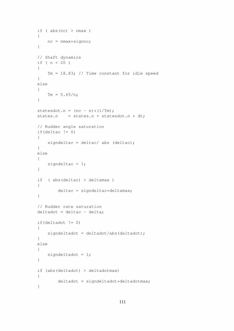
if ( abs(nc) > nmax ){

nc = nmax*signnc;}

// Shaft dynamicsif ( n < 20 ){

Tm = 18.83; // Time constant for idle speed}else{

Tm = 5.65/n;}

statesdot.n = (nc - n)*(1/Tm);states.n = states.n + statesdot.n * dt;

// Rudder angle saturationif(deltac != 0){

signdeltac = deltac/ abs (deltac);}else{

signdeltac = 1;}

if ( abs(deltac) > deltamax ){

deltac = signdeltac*deltamax;}

// Rudder rate saturationdeltadot = deltac - delta;

if(deltadot != 0){

signdeltadot = deltadot/abs(deltadot);}else{

signdeltadot = 1;}

if (abs(deltadot) > deltadotmax){

deltadot = signdeltadot*deltadotmax;}

111

statesdot.delta = deltadot;states.delta = states.delta + statesdot.delta * dt;

112

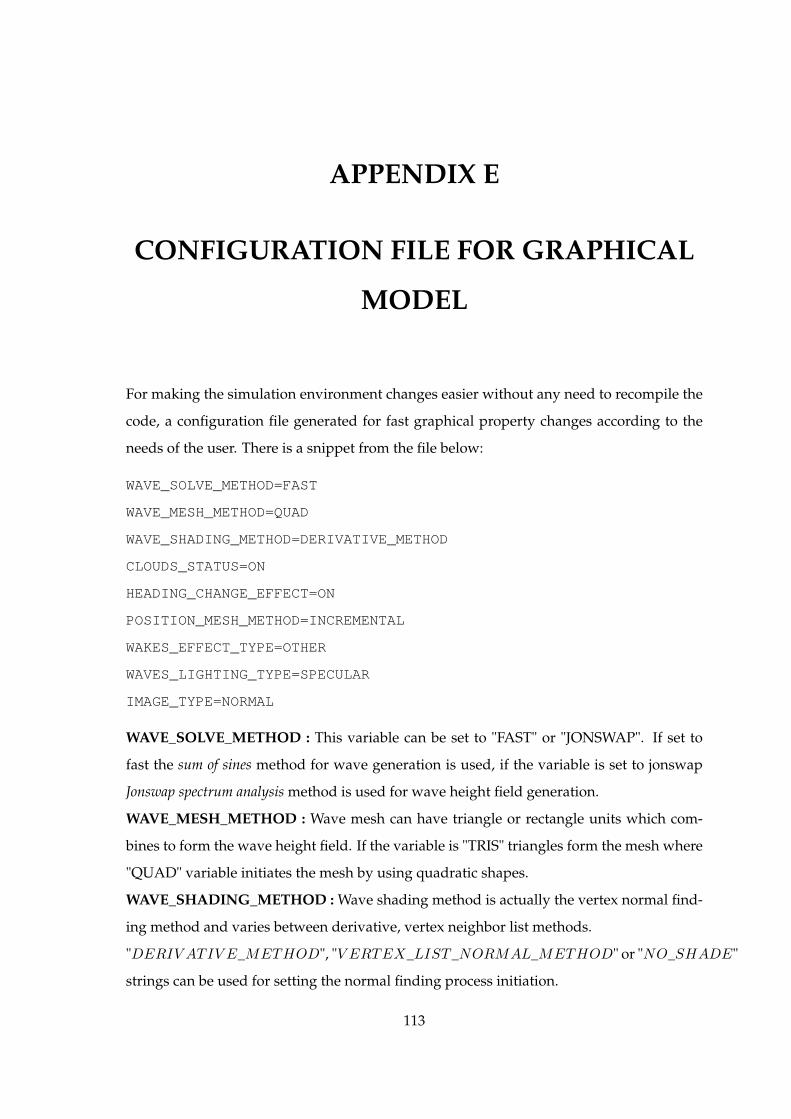
APPENDIX E

CONFIGURATION FILE FOR GRAPHICAL

MODEL

For making the simulation environment changes easier without any need to recompile the

code, a configuration file generated for fast graphical property changes according to the

needs of the user. There is a snippet from the file below:

WAVE_SOLVE_METHOD=FAST

WAVE_MESH_METHOD=QUAD

WAVE_SHADING_METHOD=DERIVATIVE_METHOD

CLOUDS_STATUS=ON

HEADING_CHANGE_EFFECT=ON

POSITION_MESH_METHOD=INCREMENTAL

WAKES_EFFECT_TYPE=OTHER

WAVES_LIGHTING_TYPE=SPECULAR

IMAGE_TYPE=NORMAL

WAVE_SOLVE_METHOD : This variable can be set to "FAST" or "JONSWAP". If set to

fast the sum of sines method for wave generation is used, if the variable is set to jonswap

Jonswap spectrum analysis method is used for wave height field generation.

WAVE_MESH_METHOD : Wave mesh can have triangle or rectangle units which com-

bines to form the wave height field. If the variable is "TRIS" triangles form the mesh where

"QUAD" variable initiates the mesh by using quadratic shapes.

WAVE_SHADING_METHOD : Wave shading method is actually the vertex normal find-

ing method and varies between derivative, vertex neighbor list methods.

"DERIV ATIV E_METHOD", "V ERTEX_LIST_NORMAL_METHOD" or "NO_SHADE"

strings can be used for setting the normal finding process initiation.

113

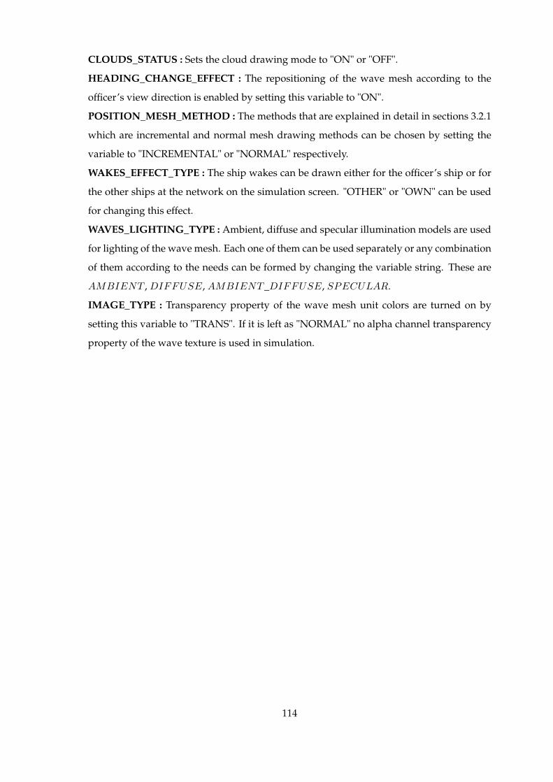
CLOUDS_STATUS : Sets the cloud drawing mode to "ON" or "OFF".

HEADING_CHANGE_EFFECT : The repositioning of the wave mesh according to the

officer’s view direction is enabled by setting this variable to "ON".

POSITION_MESH_METHOD : The methods that are explained in detail in sections 3.2.1

which are incremental and normal mesh drawing methods can be chosen by setting the

variable to "INCREMENTAL" or "NORMAL" respectively.

WAKES_EFFECT_TYPE : The ship wakes can be drawn either for the officer’s ship or for

the other ships at the network on the simulation screen. "OTHER" or "OWN" can be used

for changing this effect.

WAVES_LIGHTING_TYPE : Ambient, diffuse and specular illumination models are used

for lighting of the wave mesh. Each one of them can be used separately or any combination

of them according to the needs can be formed by changing the variable string. These are

AMBIENT , DIFFUSE, AMBIENT_DIFFUSE, SPECULAR.

IMAGE_TYPE : Transparency property of the wave mesh unit colors are turned on by

setting this variable to "TRANS". If it is left as "NORMAL" no alpha channel transparency

property of the wave texture is used in simulation.

114

APPENDIX F

USER MANUAL

In this chapter, a brief instruction set for the users of the NSTMSS system will be given. In

the first phase a configuration screen as in Figure F.1 pops up. The last three combo boxes

are added for changing the simulation abilities before initiating the graphical environment.

Wave, wake and shading properties can be selected respectively and can be eliminated

from the simulation scene in case of an extra performance need. Since all these properties

decrease the graphical and computational performance of the system, according to the

needs of the user they are enabled or not.

After initiating the simulator, the graphical properties of the scene like wave charac-

teristics or time of day properties, can be changed from a different federate which is the

Environment federate. The screen shots and introduction to that federate is given in chap-

ter 3 and section 3.3.

The keyboard and mouse usage of the system for maneuvering, is the same as the old

NSTMSS system version and user manual for simulation system can be found in [43].

115

Figure F.1: Configuration Form of NSTMSS

116

REFERENCES

[1] S. Pakkan, “Modeling and simulation of a maneuvering ship,” Master’s thesis, METU.

[2] O. Topçu and H. Oguztüzün, “Developing an HLA based naval maneuvering simula-

tion,” Naval Engineers Journal by American Society of Naval Engineers (ASNE), vol. 117,

pp. 23–40, 1 2005.

[3] “http://www.ljmu.ac.uk/lairdsidemaritimecentre/,” Lairside Maritime Center.

[4] “http://www.amhrc.edu.au/,” Australian Maritime Hydrodynamics Research Centre.

[5] J. Tessendorf, “Simulating ocean water,” SIGGRAPH Course Notes, 1999.

[6] N. L. Max, “Vectorized procedural models for natural terrain: Waves and islands in

the sunset,” in SIGGRAPH ’81: Proceedings of the 8th annual conference on Computer

graphics and interactive techniques, (New York, NY, USA), pp. 317–324, ACM, 1981.

[7] G. A. Mastin, P. A. Watterberg, and J. F. Mareda, “Fourier synthesis of ocean scenes,”

IEEE Comput. Graph. Appl., vol. 7, no. 3, pp. 16–23, 1987.

[8] A. Fournier and W. T. Reeves, “A simple model of ocean waves,” SIGGRAPH Comput.

Graph., vol. 20, no. 4, pp. 75–84, 1986.

[9] D. R. Peachey, “Modeling waves and surf,” SIGGRAPH Comput. Graph., vol. 20, no. 4,

pp. 65–74, 1986.

[10] H. He, H. Liu, F. Zeng, and G. Yang, “A way to real-time ocean wave simulation,” in

CGIV ’05: Proceedings of the International Conference on Computer Graphics, Imaging and

Visualization (CGIV’05), (Washington, DC, USA), pp. 409–415, IEEE Computer Society,

2005.

[11] A. T. Layton and M. van de Panne, “A numerically efficient and stable algorithm for

animating water waves,” vol. 18, (Berlin / Heidelberg), pp. 41–53, Springer, 2 2002.

117

[12] J. X. Chen and N. da Vitoria Lobo, “Toward interactive-rate simulation of fluids with

moving obstacles using navier-stokes equations,” Graph. Models Image Process., vol. 57,

no. 2, pp. 107–116, 1995.

[13] X. Yingqing, S. Cheng, L. Hua, and L. Shenquan, “Physically based simulating of wa-

ter currents and waves,” Chinese J. Computers, 1996.

[14] Y. Huai-Ping and S. Jia-guang, “Wave simulation based on ocean wave spectrums,”

Journal of System Simulation, 2002.

[15] A. Osman and H. Ammar, “Parallel analysis and implementation of large eddy simu-

lations of ship wakes,” 2006.

[16] T. Mäki-Patola, “Extendable virtual environment visualization system for networked

naval simulation,” Master’s thesis, Helsinki University of Technology, Espoo, Finland,

2002.

[17] J. L. Meriam and L. G. Kraige, Engineering Mechanics: Dynamics, vol. 2. New York:

John Wiley & Sons Ltd, 3 ed., 1993.

[18] J. P. Strand, Nonlinear Position Control Systems Design for Marine Vessels. PhD thesis,

Norwegian University of Science & Technology, Trondheim, Norway, 1999.

[19] K. P. Lindegaard, Acceleration Feedback in Dynamic Positioning. PhD thesis, Norwegian

University of Science & Technology, Trondheim, Norway, 2003.

[20] T. Holzühter, “LQG approach for the high-precision track control of ships,” in Control

Theory and Applications, vol. 144, pp. 122–127, 1997.

[21] E. Lefeber, K. Y. Pettersen, and H. Numeijer, “Tracking control of an underactuated

ship,” in IEEE Trans. Contr. Sys. Tech., vol. 11, pp. 52–61, 2003.

[22] T. Fossen, Guidance and Control of Ocean Vehicles. England: John Wiley & Sons Ltd.,

1994.

[23] K. S. M. Davidson and L. I. Schiff, “Turning and course keeping qualities,” in Trans.

Soc. of Nav. Architects Marine Eng., vol. 54, pp. 152–200, 1946.

[24] Nomoto, K. Taguchi, K. Honda, and Hirano, “On the steering qualities of ships,” tech.

rep., Shipbuilding Progress, 1957.

118

[25] D. Clarke, “The foundations of steering and manoeuvring,” in IFAC Conf. Manoeuver-

ing and Control of Marine Crafts, IFAC, (Girona, Spain), 2003.

[26] T. I. Fossen, Marine Control Systems: Guidance, Navigation, and Control of Ships. Trod-

heim, Norway: Marine Cybernetics, 2002.

[27] J. Dahmann, “High level architecture for simulation,” Defense Modeling and Simulation

Office, 1998.

[28] M. Finch, Efective Water Simulation from Physical Models. GPU Gems, 2004.

[29] M. Gomez, Interactive Simulation of Water Surfaces, pp. 187–194. Charles River Media,

2000.

[30] T. Pérez and M. Blanke, “Mathematical ship modeling for control applications,” tech.

rep., Technical University of Denmark, 2000.

[31] J. Newman, Marine Hydrodynamics. Cambridge: MIT Press, 1977.

[32] D. Sicuro, “Physically based modeling and simulation of a ship in open water 3d vir-

tual environment,” Master’s thesis, California, 2003.

[33] A. H. Techet, “Lecture notes for 13.42, lecture 6,” in Design Principles for Ocean Vehicles,

MIT OpenCourseWare, 2005.

[34] X. Cui, J. Yi-cheng, and L. Xiu-wen, “Real-time ocean wave in multi-channel marine

simulator,” in VRCAI ’04: Proceedings of the 2004 ACM SIGGRAPH international confer-

ence on Virtual Reality continuum and its applications in industry, (New York, NY, USA),

pp. 332–335, ACM, 2004.

[35] Hinsinger, Damien, Neyret, Fabrice, Cani, and Marie-Paule, “Interactive animation of

ocean waves,” in ACMSIGGRAPH/EG Symposium on Computer Animation (SCA), july

2002.

[36] H. Gouraud, “Continuous shading of curved surfaces,” IEEE Transactions on Comput-

ers, vol. 20, pp. 623–629, 6 1971.

[37] M. Zyda, D. Pratt, J. Falby, and P. Baraham, “NPSNET: A network software architec-

ture for large-scale virtual environments,” vol. 2, no. 3, 1993.

119

[38] J. A. Nobles and J. F. Garrova, “Design and implementation of real-time deployable

three dimensional shiphandling training simulator,” Master’s thesis, Naval Postgrad-

uate School, Montery California, June 1995.

[39] R. Munro-Smith, Notes and Examples in Naval Architecture. London: Edword Arnold

Publishers Ltd., 1965.

[40] S. N. Blagoveschcensky, Theory of Ship Motions. NewYork: Dover Publications Inc.,

1962.

[41] S. G. Inc., OpenGL Performer Getting Started Guide, 007-3560-002 ed., November 2000.

[42] D. Modeling and S. OfficeDMSO, High Level Architecture RunTime Infrastructure RTI

1.3Next Generation Programmer’s Guide Version 6, 2000.

[43] “http://www.ceng.metu.edu.tr/ otopcu/nstmss/,” NSTMSS Home Page.

120