Dynamic Matrix Flight Control design for a nonlinear ...tjeas.com/wp-content/uploads/2013/10/2880-2891.pdf · Dynamic Matrix Flight Control design for a nonlinear missile Autopilot

Technical Journal of Engineering and Applied Sciences Available online at www.tjeas.com ©2013 TJEAS Journal-2013-3-21/2880-2891 ISSN 2051-0853 ©2013 TJEAS

Dynamic Matrix Flight Control design for a nonlinear missile Autopilot

A.Ahari A1*, Torabi A, Karsaz A2

Khorasan Institute of Higher Education, Mashhad, Iran

Corresponding author: A. Ahari A

ABSTRACT: Nonlinear control problem for a missile autopilot is quick adaptation and minimizing the desired acceleration to missile nonlinear model. For this several missile controllers are provided which are on the basis of nonlinear control or design of linear control for the linear missile system. In this paper a linear control of dynamic matrix type is proposed for the linear model of missile. In the first section, an approximate two degrees of freedom missile model, known as Horton model, is introduced. Then, the nonlinear model is converted into observable and controllable model base on the feedback linear rule of input-state mode type. Finally for design of control model, the dynamic matrix flight control, which is one of the linear predictive control design methods on the basis of system step response information, is used. This controller is a recursive method which calculates the development of system input by definition and optimization of a cost function and using system dynamic matrix. So based on the applied inputs and previous output information, the missile acceleration would be calculated. Unlike other controllers, this controller doesn’t require an interaction effect and accurate model. Although, it has predicting and controlling horizon, there isn’t such horizons in non-predictive methods. Keywords: Dynamic Matrix Control (DMC), 2 degrees of freedom missiles model, Feedback linearization, Flight control

INTRODUCTION

The performance of aerospace systems such as aircraft, spacecraft and missiles is highly dependent on the capabilities of the guidance, navigation and control systems. To achieve improved performance in such aerospace systems, it is important that more sophisticated control systems be developed and implemented (Tsourdos & White, 2005). Modern missiles often operate in flight regimes where nonlinearities significantly affect dynamic response. For example, a high performance missile must be quickly responsive to and follow accurately any guidance commands, so that, it can intercept fast moving and agile targets (Bryson & Y-C 1975; Xin & Balakrishnan, 2003). The tracking performance of a missile is also dependent on the location within the flight envelope and varies with factors such as Mach number and dynamic pressure. Many nonlinear control methods have been proposed for the missile autopilot design. Several approaches, including adaptive control (Lin & Cloutier, 1991), nonlinear control (White et al., 1998), and gain scheduling (Shamma & Cloutier, 1993) have been used to alleviate these tracking problems. In this paper, input-state linearization method is used for linearization. Feedback linearization is a popular method used in nonlinear control applications, and there have been several flight control demonstrations (Snell, 1992). Feedback linearization methods can be viewed as the ways of algebraically transforming a nonlinear system dynamic, fully or partially, into a simple linear one. In the standard approach to exact input-state linearization, one uses coordinate transformation and static state feedback such that the closed-loop system, in the defined region, takes a linear canonical form (Cheh et al., 2004). The input-state linearization method differs from conventional linearization techniques in that input-state linearization is achieved via exact state transformations and feedback, rather than by linear approximations of the system dynamics. Linearization has a number of advantages in the control field, including simplicity, being easily implemented, being well developed, and so forth, and thus the literature contains many studies of the linearization of both discrete time systems and continuous-time systems (Fuh, 2009). After the system’s linearization form is obtained, the linear control design scheme is employed to achieve stabilization or tracking (Slotine,1991). Model predictive control designates a wide range of control methods which make an explicit use of a model of the process to obtain the control signal by minimizing an objective function. The common idea is

Tech J Engin & App Sci., 3 (21): 2880-2891, 2013

2881

receding strategy which means that, the objective function is minimized by considering also future control actions along the so-called prediction horizon but only the first control signal is applied to the system; then the horizon is displaced towards the future and the next control signal is recalculated. In view of the main idea of the model predictive control strategy it is clear that, the process model plays an important role in the method. There are many types of models used; one of them is the so-called step response model. For stable systems one may take a truncated response and with this model the control signal can be calculated by minimizing the objective function along the prediction horizon. The step response model is used by the Dynamic Matrix Control (DMC) algorithm, developed at the end of the seventies (Cutler & Ramaker, 1979 and 1980). It is a successful and widely applying technique in industrial and engineering applications (Besnyei & Simon, 2010). The dynamic matrix control is one of the important and representative predictive control algorithms and characterized by replacing the traditional auto correction of single step prediction with multiple step prediction, repeating optimization based on the practical feedback information, and restraining the algorithm sensitivity to parameter change of the model effectively (LU & TSA, 2007; Yao & Guo, 2006; Guo et al., 2010). The purpose of this paper is to find a control rule for a nonlinear missile, so that, by applying it, the desired acceleration of the missile be obtainable. Several controllers for this nonlinear missile model have been proposed which present a combination of feedback linearization methods or local linearization with linear, adaptive and intelligent controllers. For this model, the adaptive controller by varying parameters of the missile condition (Tsourdos & White, 2005), multi-objective fuzzy controller (Tsourdos et al., 2006), variable gain fuzzy controller (Tabataba et al., 2010) and quasi-LPV controller are designed, which these controllers are designed using the input - output feedback linearization or local linearization (White et al., 2007). This paper presents a dynamic matrix controller which is the controller for model missile. Due to the predictive and controllable horizons, which aren’t expressed in unpredictable controllers, this algorithm is not comparable with unpredictable methods. However, due to its simplicity and good performance of the algorithm compared to other predictive algorithms, designers apply this algorithm to design the controller. For example, the model algorithm control (MAC), which is based on the impulse response, has two main problems, one of them is lack of accurate impulse response in operational systems, and the other is the designed control signal due to lack of control effort in inaccurate cost function. Another method of widely used predictive method is the Generalized Predictive Control (GPC), which is on the basis of the discrete transfer function model of the system. This method is generalized method of two previous ones, which get better results than the previous methods, but heavy calculations of this method prevents from simple design for complex systems. In the first part of this paper, the nonlinear models and design of linearization rule and linearization method of input - state are discussed. In this linearization, one of the problems of designing a linearization rule which is changes of the aerodynamic coefficients based on the parameters such as Mach number and angle of attack is resolved. Furthermore, the dynamic matrix control for step response of linear system which has limited final value is designed. Simulation results show that, the designed linear rule was succeeded and the applied dynamic matrix control has a suitable and robust adaptation for the missile acceleration. Missile model The missile model used in this study derives from a nonlinear model produced by Horton of Matra-British Aerospace (Horton, 1992). This study will look at the reduced problem of a 2 DOF controller for the pitch and yaw planes without roll coupling. This model describes a reasonably realistic airframe of a tail controlled tactical missile in the cruciform fin configuration (Fig.1). The angular and translational equations of motion of the missile airframe are given by

0 0

1

0 0

1

2

1 1

2 2

yv y

z nr nv n

v V S C v V C Urm

r I V Sd dC r C v V C

(1)

where the variables are defined in Fig. 1, Table 1 and 2.


2882

Figure 1. Airframe axes.

In Eq. (1), v is the sideslip velocity, U is the longitudinal velocity, r is the body rate, δ is the rudder fin

deflections, V0 is total velocity vector and calculated from 2 2U v and V0≈U because U>>v, Cyv, Cyδ is lateral

force coefficient due to sideslip velocity and fin angle, Cnr, Cnv, Cnδ is yawing moment coefficient due to body rate, sideslip velocity and fin angle. These forces and moments are derived from wind tunnel measurements and by using polynomial approximation algorithms which can be fitted to the set of curves taken from look-up tables for different flight conditions (Tsourdos & White, 2000). A detailed description of this model can be found in Horton (1992) found that some of them are shown in Table 1.

Table 1.

Force and moment coefficients of missile model

yvC

0.5 25 60 1 cos 4

26 1.5 30 1 cos 4

M

M

yC

10 0.5 1.6 2 1 cos 4

1.4 1.5 1 cos 4

M

M

nrC 500 30 200M

nvC

1

,

1.3 0.1 0.2 1 cos 4

0.3 1 cos 4 (1.3 )500

m yv

m

S C where

S d M

m

nC

1

,

2.6 (1.3 )500

f y

f

S C where

mS d

These force and moment coefficients depending on parameters such as λ, Mach number and σ. λ is roll angle, The Mach number is defined as M=V0/a where a is the speed of sound. σ is incidence angle or the

angle between U and 0V , can be taken as σ=v/V0, as sinσ≈σ for small σ (Tsourdos et al. 2006). Involving the

Mach number 0.6 6M , roll angle 4.5 45o o and total incidence 3 30o o

(White et al. 2006). In Table 2

the characteristics of the Horton model are presented.


2883

Table 2.

Characteristics of the Horton model

0 Sea level air density 31.23Kg m

Air density 0 0.094h

h Altitude in Km

0a

Sea level velocity of sound 340m s

a Velocity of sound 0 4a a h m s

d Reference diameter (calibre) 0.2m

S Reference area 2 24 0.0314d m

l Length of the missile 2.7m

m Mass 125Kg

zI Lateral inertia 275Kgm

mS

Static margin (body+wings) cp cgx x

fS

Fin moment arm for lateral motion f cgx x

fx Centre of pressure (fins only) 2.6 m

cpx Centre of pressure (body+wings)

1.3 0.1 0.2cpx M

cgx Centre of gravity 1.55m

Input – State linear feedback The standard form of the nonlinear system can be written as

( ) ( )x f x g x (2)

where f(x) and g(x) are smooth vector fields on nR . If the state vector is defined as x=[v r]T, then Eq. (1)

can be rewritten in the standard form as in Eq. (2) with the vector fields defined as follows:

0

1

0

2

0

1 2

0

1

2( )

1 1( )

2 2

1

2( )

1

2

yv

y nr nv

y

y n

V SC v Urm

f x

I V Sd dC r C v

V SCm

g x

I V SdC

(3)

Definition 1. A nonlinear system in the form of Eq.(2) is said to be input-state linearizable if there is a region Ω in R

n, a diffeomorphism Φ: Ω→R

n, and a nonlinear feedback control law and defining a new input as

(Slotine, 1991):

( , ) ( , )v r v r u (4)

Such that the new state variables Z= Φ(x) and the new input u satisfy a linear time-invariant relation:

Z AZ Bu (5)

where u is new input or linear model input, the new state Z is called the linearizing state, and the control law (4) is called the linearizing control law. By the above definition, the fundamental results of feedback linearization can be used to linearize the system. Select the matrix A and B as

0 1 0

0 0 1A B

(6)

Linear system is controllable and observable. Expanding Eq. (5), we obtain


2884

1 12

2 2

( ) ( ) 0

( ) 0 ( )

z zf x z g x

x x

z zf x g x u

x x

(7)

Since z1, z2 are independent of ξ, so α(v,r), β(v,r) is calculated as

12 22 2

1 22

2 211 11 2

2

2 211 11 2

2

1 1

Fz z z zF FFv r v r

z zGz z G Gv rGv r

z zGz z G Gv rGv r

(8)

where

1 0 0

1

2 0 0

2

1 0 0

1 2

2 0 0

1, , ,

2

1 1, , , , ( )

2 2

1,

2

1,

2

yv yv

nv nr y nr nv

y y

n y n

F C V v r V SC v Urm

F C C V v r I V Sd dC r C v

G C V V SCm

G C V I V SdC

(9)

Assuming the z1=v then

12 1 2

2

G

z F FG

(10)

With z2 be calculated the following relationships.

1 2 22 1 2 1 2

2 1

2

2

21 2

2 1 1 1 2

2

2 2

G F GF G G G F

z F v v v

v v G

FG G

z F F G Fr

r r G r G r

(11)

It should be noted that Cyv, Cyδ, Cnr, Cnv, Cnδ are related to M, σ that M, σ is related to v. Some derivatives as

0

2 2

2 2

2 2

22 2

2 2 3

0

2

3

0

2

3

0

1

( )

0

0

V v

v U v

M v

v a aU v

vU v

UU v

v U v V

Uv

V

v Uv

V

(12)

If force and moment coefficients is defined as


2885

0

0

10

500 30 200

yv yv yvM yv

y y M y

nr

m m mM m

nv m yv

n f y

C C C M C

C C M C

C M

S S S M S

C S C

C S C

(13)

Then derivatives are as follows.

30 200

yv

yvM yv

y

y M y

nr

mmM m

yvnv myv m

n

f y M y

CC C

v a v

CC C

v a v

C

v a v

SS S

v a v

CC SC S

v v v

CS C C

v a v

(14)

Using the Eqs (8) to (15) α, β can be calculated. Missile acceleration is second state of linear model and it is calculated as

0 1

y CZ

C

(15)

In this linearization, due to taking into account the effect of aerodynamic coefficients in the equations of the linear rule, the effect of these parameters on the model output can be neglected. In a previous study (Tsourdos & White, 2005), the designed linear rule of input - output has been calculated with the assumption of constant aerodynamic coefficients and regardless of the effect of missile conditions on these parameters. This proposed control rule solves one of the main problems of missile controlling which is the change of aerodynamic coefficients. The other effective parameters in this model such as changes in mass, air pressure, Inertia, etc. can be removed by a time-varying gain or a smart filter. Step Responses For designing DMC controller, step response is required. Linear system transfer function is as follows:

( ) 1

( )

y s

u s s (16)

According to Eq. (16), the output step response of the linear system seen in Fig 2.

Figure 2. Step responses for linear missile acceleration


2886

It is difficult to design DMC controller, because transfer function has poles on the jω axis. To remove ramp of the step responses, the feedback is used as follows.

2

0 10

0 0Z Z B u k Z

(17)

Assuming k2=5, then step responses figures is presented in Fig 3.

Figure 3. Step responses with state feedback for linear model

Dynamic Matrix Flight Control DMC is a control based optimization methodology that is explicitly utilized in dynamic mathematical model of a process to obtain a signal which minimizes the objective function. The advantages of this controller include: controlling sensitivity to time delay, interaction with other states on output and good resistance to noise input due to the recursive algorithm which is the superiority of this controller compared to other linear controllers in linear processes. This model which uses the step response of a system to design a cost function, describes the system perfectly (Paulusová & Dúbravská 2010, Bemporad & Morari 1999, Carlos et al. 1989). The model must describe the system well. The future process outputs y(k+i) for i=1,….,p are predicted over the prediction horizon (p) using a model of the process. These values depend on the current process state and on the future control signals u(k+i) for i=0,….,m-1 over the control horizon (m), where m≤p. The control variable is manipulated only within the control horizon and remains constant afterwards, u(k+i)=u(k+m-1) for i=m,….,p-1. Process interactions and dead times can be intrinsically handled with model predictive control schemes such as DMC (Paulusová & Dúbravská 2010, Bemporad & Morari 1999, Carlos et al. 1989). The principle of DMC is shown in Fig. 4. A general objective function is the following quadratic form

T

T

d p d pJ y y Q y y U R U (18)

Fig ure4. The principle of DMC

where, yd is desired set point, R and Q are weight identity matrix, p and m are length of the prediction horizon and control horizon, Δu(k) is change in manipulation variable and calculated as

( ) ( ) ( 1)u k u k u k (19)

yp is the process output, at sample instant is given as


2887

1

( ) ( 1)p i

i

y k g u k

(20)

where gi is step response coefficients. By minimizing objective function, the optimal solution is then given in matrix form as:

1

T TU G QG R G QE

(21)

where G is dynamic matrix and constructed as

1

2 1

1 1

1 1

0 ... 0

... 0

...

...

m m

p p p m

g

g g

Gg g g

g g g

(22)

and E is defined as

d pastE y y D (23)

In Eq (23), D is disturbances are considered to be constant between sample instants which can be removed by filter as

1

1( )

1f z

z

(24)

where γ is between 0 and 1. ypast in Eq (23) is calculated as

1

1past DMC Ny G U U g

(25)

where, gN+1 is final value of step response and G- constructed as

Figure 5. Proposed flight control scheme for tracking based on DMC.

2 3 1

3 4 0

0 0

N N

N

p m N

g g g g

g g gG

g g

(26)

In the previous equations, matrix elements of the ΔU, ΔU- and U as

( ) ( 1) ( 1)

( 1) ( 2) ( 1)

( ) ( 1) ( 1)

T

T

T

DMC

U u k u k u k m

U u k u k u k N

U u k N u k N u k N p

(27)

Optimal input in present time as

( ) ( 1) ( )u k u k u k (28)

SIMULATION RESULTS For simulation, the desired output applied in the following equation:

x

0

mad dy d yt

(29)


2888

where ydmax is a maximum value for yd. This relationship must be applied to model assumptions. Parameters for DMC are assumed as:

25 5

0.5 0.5p p m m

p m

R I Q I

(30

)

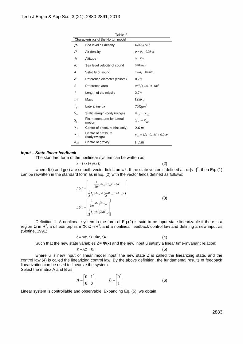
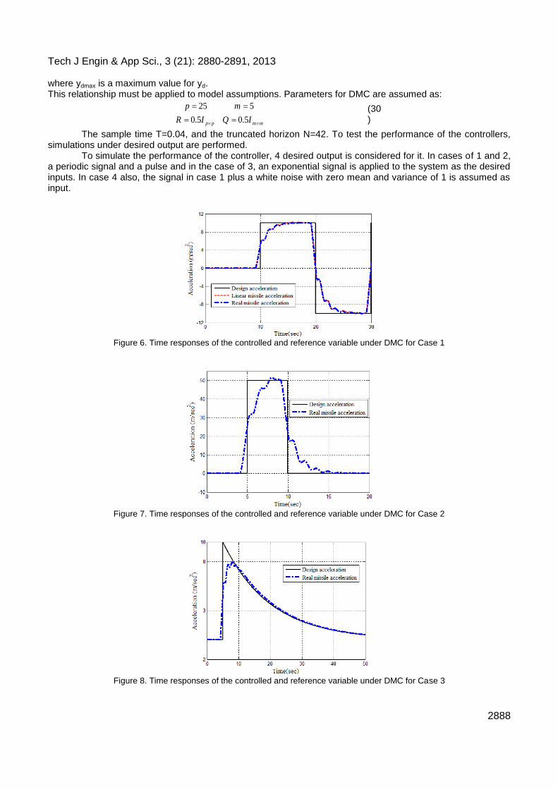
The sample time T=0.04, and the truncated horizon N=42. To test the performance of the controllers, simulations under desired output are performed. To simulate the performance of the controller, 4 desired output is considered for it. In cases of 1 and 2, a periodic signal and a pulse and in the case of 3, an exponential signal is applied to the system as the desired inputs. In case 4 also, the signal in case 1 plus a white noise with zero mean and variance of 1 is assumed as input.

Figure 6. Time responses of the controlled and reference variable under DMC for Case 1




2889

Figure 9. States of nonlinear and linear models with rudder and linear model input for Case 1


2890


CONCLUSION

In this paper, for the first time the idea of DMC controllers for flight control of a missile which has nonlinear performance is implemented. In this controller, the step response model is defined as a parametric model and it is used for the design and optimization of the cost function and optimal selection of inputs . The advantages of this method are its easy implementation compared with the adaptive methods and lack of sensitivity to the interaction and its performance for the acceleration response of the missile. Computer simulation results of the missile show that for intercept of the target point, the proposed method has a good performance. The resistance to noise of the proposed method under these constraints is quite visible, although it has a poor function in ramp response, but this problem is solved with a feedback mode model. Due to incorporate the aerodynamic coefficients as a function of lateral velocity of missile, the designed control law has proper and accurate performance which observed in Fig. 6 & 9.

REFERENCES

Bemporad A, Morari M.1999. "Robust Model Predictive Control: A Survey". Robustness in identification and control. Volume 245, Springer,

1999. Besnyei A, Simon LP.2010. "Asymptotic output controllability via dynamic matrix control". Mathematics subject classification 34H05,

93B05. Bryson AEJr, Ho YC.1975. "Applied optimal control" . Hemisphere, Washington DC. Carlos E, Garcia D, Prett M, Morari M.1989. "Model Predictive Control: Theory and Practice a Survey". Automatica, Vol. 25, (Issue

3), 1989, pp. 335-348. Chen CK, LinCJ, Yao LC.2004. "Input-state linearization of a rotary inverted pendulum". Asian Journal of Control, Vol. 6, No. 1, pp.130-135. Cutler CR, Ramaker BL.1980. "Dynamic Matrix Control a computer control algorithm". Automatic Control Conference, San Francisco. Cutler CR, Ramaker BL.1979. "Dynamic Matrix Control a computer control algorithm". AICHE National Meeting, Houston. Fuh CC.2009. "Optimal control of chaotic systems with input saturation using an input-state linearization scheme". Commun Nonlinear Sci

Numer Simulat 14 .3424–3431. Guo W, Wen J. Zhou W.2010. "Fractional-order PID Dynamic Matrix Control Algorithm based on Time Domain". Proceedings of the 8th

World Congress on Intelligent Control and Automation July 6-9, Jinan, China. Horton M.1992. "A study of autopilots for the adaptive control of tactical guided missiles". Master’s thesis, University of Bath. Lin C, Cloutier J .1991. "High performance, adaptive, robust bank-to-turn missile autopilot". In AIAA guidance, navigation, control

conference (pp. 123–137). LU CH, TSA ICC .2007. "Generalized predictive control using recurrent fuzzy neural networks for industrial process". Journal of Process

Control , 17(1):83-92. Paulusová J, Dúbravská M.2010. "Predictive control of nonlinear process". International Conference Cybernetics and Informatics. Shamma J, Cloutier J.1993. "Gain-scheduled missile autopilot design using lpv transformations". Journal of Guidance, Control and

Dynamics. Slotine JE, Li WP.1991. "Applied Nonlinear Control". Prentice-Hall, NJ. Snell .1992. "Nonlinear inversion flight control for a super maneuverable aircraft". Journal of Guidance, Control and Dynamics,15(4), 976–

984. Tabatabaei S, Tohidi S, Sadeghi M, Mirjafari PS. 2010." Fuzzy Self-Tuning Gain Scheduled Control Design for an Autopilot Missile".

International Conference on Computer Applications and Industrial Electronics (ICCAIE 2010), December 5-7, 2010, Kuala Lumpur, Malaysia.

Tsourdos A, Hughes EJ, White BA.2006. "Fuzzy multi-objective design for a lateral missile autopilot". Control Engineering Practice 14, 547–561.

Tsourdos A, White BA .2000. "Pseudolinearising autopilot for a 6 dof quasi-linear parameter varying missile model". International Conference on Control Applications. Proceedings of the IEEE .

Tsourdos A, White BA.2005. "Adaptive flight control design for nonlinear missile". Control Engineering Practice 13, 373–382. White BA, Bruyer L, Tsourdos A .2007. "Missile autopilot Design using Quasi-LPV polynomial eigenstructure assignment". IEEE

Transactions On Aerospace and Electronic Systems Vol. 43, NO. 4.


2891

White BA, Tsourdos A, Blumel A .1998. "Lateral acceleration control design of a nonlinear homing missile". In Fourth IFAC nonlinear control systems design symposium (pp. 708–713).

Xin M, Balakrishnan SN.2003. "Missile longitudinal autopilot design using a new suboptimal nonlinear control method". IEE Proc Control Theory Appl, Vol. 150, No. 6.

Yao W, Guo W.2006. "Probabilistic constrains into algorithm of dynamic matrix control". Journal of Wuhan University of Technology, 28(8):100-103.

Documents

Dynamic Matrix Flight Control design for a nonlinear ...tjeas.com/wp-content/uploads/2013/10/2880-2891.pdf · Dynamic Matrix Flight Control design for a nonlinear missile Autopilot