Dynamic Local Scheduling of Multiple DAGs in Distributed

Dynamic Local Scheduling of Multiple DAGs inDistributed Heterogeneous Systems

Ondrej Votava, Peter Macejko, and Jan Janecek

Czech Technical University in Prague{votavon1, macejp1, janecek}@fel.cvut.cz

http://cs.fel.cvut.cz

Dynamic Local Scheduling of Multiple DAGs inDistributed Heterogeneous Systems

Ondrej Votava, Peter Macejko, and Jan Janecek1

Czech Technical University in Prague{votavon1, macejp1, janecek}@fel.cvut.cz

http://cs.fel.cvut.cz

Abstract. Heterogeneous computational platform offers a great ratiobetween the computational power and the price of the system. Staticand dynamic scheduling methods offer a good way of how to use thesesystems efficiently and therefore many algorithms were proposed in theliterature in past years. The aim of this article is to present the dynamic(on-line) algorithm which schedules multiple DAG applications withoutany central node and the schedule is created only with the knowledge ofnode’s network neigbourhood. The algorithm achieves great level of fair-ness for more DAGs and total computation time is close to the standardand well known competitors.

1 Introduction

Homogeneous (heterogeneous) computational platform consists of a set of iden-tical (different) computers connected by a high speed communication network[1, 2]. Research has been done last few years on how to use these platforms ef-ficiently [3–5]. It is believed that scheduling is a good way on how to use thecomputation capacity these systems offer [1, 6]. Traditional attitude is to pre-pare the schedule before the computation begins [7, 8]. This requires informationabout the network topology and parameters and also node’s computational abil-ities. Knowing all of this information we can use the static (offline) schedulingalgorithm. Finding the optimal value of makespan – i.e. the time of the com-putation in total – is claimed to be NP complete [9, 10]. Therefore research hasbeen done and many heuristics have been found [11, 12].

Compared to static scheduling, dynamic (online) scheduling allows us tocreate the schedule as part of the computation process. This allows dynamicalgorithms to use the feedback of the system and modify the schedule in accor-dance with current state of the system. Dynamic algorithms are often used forscheduling multiple applications [13–16] at the same time and therefore fairnessof generated schedules is important.

The algorithm presented in this paper does not require the global knowledgeof the network, it uses the information gathered from node’s neighbors only.The phase of creating the schedule is fixed part of the computation cycle. Thealgorithm is intended to be used for scheduling more DAGs simultaneously andtries to achieve fair division of tasks for all computing nodes.

M. Necasky, J. Pokorny, P. Moravec (Eds.): Dateso 2015, pp. 1–12, CEUR-WS.org/Vol-1343.

2 Ondrej Votava, Peter Macejko, Jan Janecek2 Ondrej Votava et al.

The structure of this article, which is the enhanced version of [17], is asfollows, in the section two we describe the problem of scheduling and make abrief summary of related work. In the section three we describe the algorithmitself and in the following section we describe the testing environment and resultswe obtained by running several simulations. In the fifth section we conclude theresults from section four, show the pros and cons of the presented algorithm anddiscuss the future improvements.

2 Problem definition

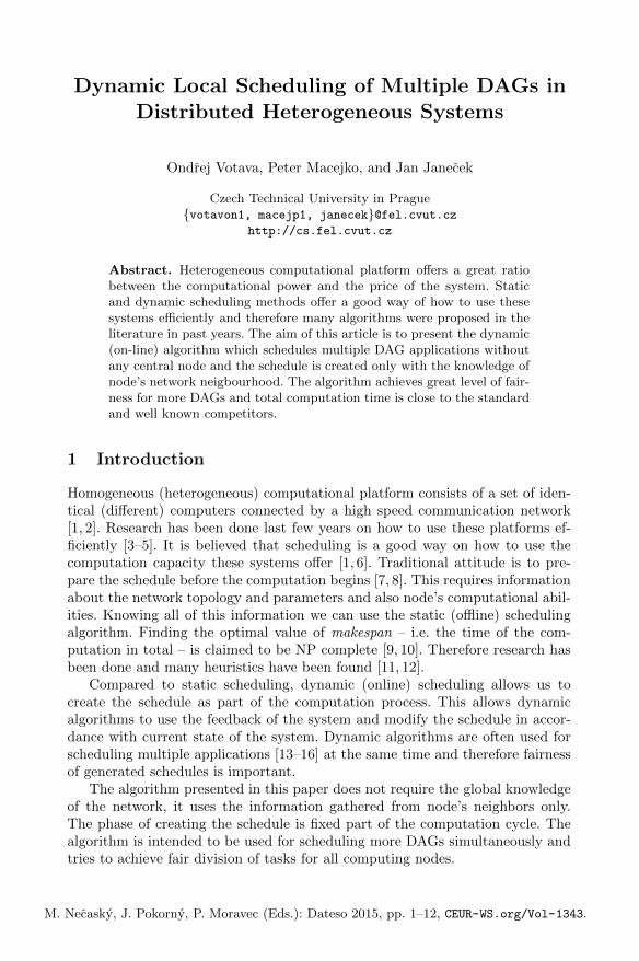
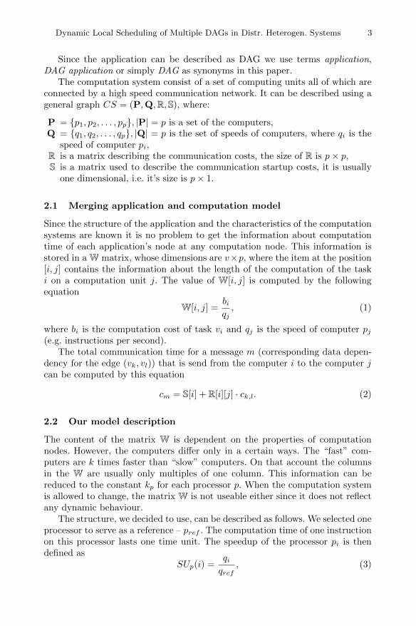
The application model can be described as a directed acyclic graph AM = (V,E,B,C)[12, 18], where:

V = {v1, v2, . . . , vv}, |V| = v is the set of tasks, task vi ∈ V represents thepiece of code that has to be executed sequentially on the same machine,

E = {e1, e2, . . . , ee}, |E| = e is the set of edges, the edge ej = (vk, vl) representsdata dependencies, i.e. the task vl cannot start the computation until thedata from task vk has been received, task vk is called the parent of vl, vl iscalled the child of vk,

B = {b1, b2, . . . , bv}, |B| = v is the set of computation costs (e.g. number ofinstructions), where bi ∈ B is the computation cost for the task vi,

C = {c1, c2, . . . , ce}, |C| = e is the set of data dependency costs, where cj = ck,lis the data dependency cost (e.g. amount of data) corresponding to the edgeej = (vk, vl).

The task which has no parents or children is called entry or exit task respec-tively. If there are more than one entry/exit tasks in the graph a new virtualentry/exit task can be added to the graph. Such a task would have zero weightand would be connected by zero weight edges to the real entry/exit tasks.

c

b

i

i

i,j

j

b j

entry

exit

1 2 3

4 5 6 7

8 9 10

00

10 3020

251426

3637

40 25 36 57

88 49 11

48

58

5169

0 0

000

Fig. 1. Application can be describedusing DAG.

p1

p2

p3

p5

p8

p76

p

p4

Fig. 2. The computation system can berepresented as a general graph.

Dynamic Local Scheduling of Multiple DAGs in Distr. Heterogen. Systems 3Dynamic Local Scheduling of Multiple DAGs in Distr. Heterogen. Systems 3

Since the application can be described as DAG we use terms application,DAG application or simply DAG as synonyms in this paper.

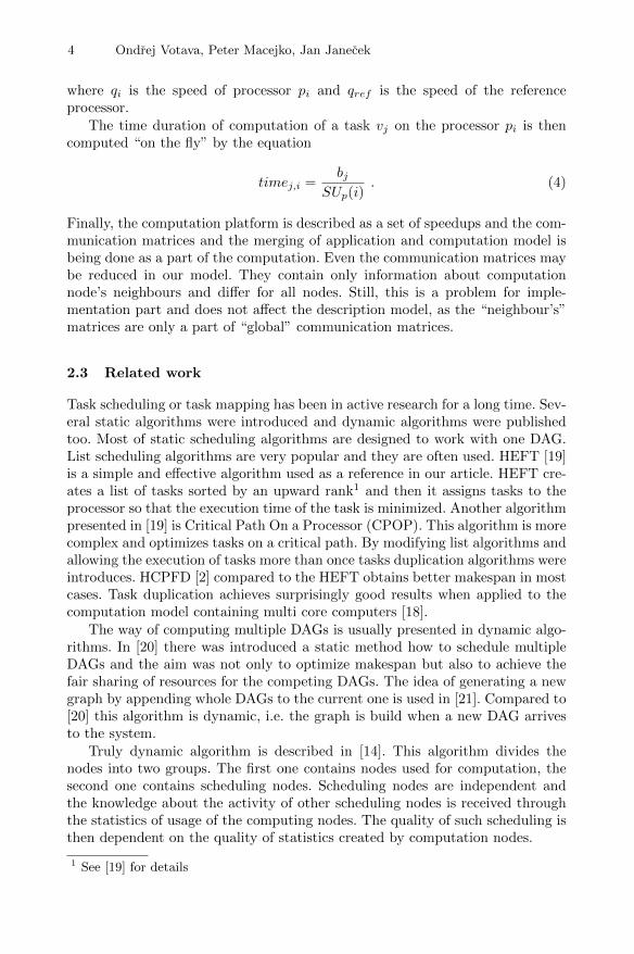
The computation system consist of a set of computing units all of which areconnected by a high speed communication network. It can be described using ageneral graph CS = (P,Q,R,S), where:

P = {p1, p2, . . . , pp}, |P| = p is a set of the computers,Q = {q1, q2, . . . , qp}, |Q| = p is the set of speeds of computers, where qi is the

speed of computer pi,R is a matrix describing the communication costs, the size of R is p× p,S is a matrix used to describe the communication startup costs, it is usually

one dimensional, i.e. it’s size is p× 1.

2.1 Merging application and computation model

Since the structure of the application and the characteristics of the computationsystems are known it is no problem to get the information about computationtime of each application’s node at any computation node. This information isstored in a W matrix, whose dimensions are v×p, where the item at the position[i, j] contains the information about the length of the computation of the taski on a computation unit j. The value of W[i, j] is computed by the followingequation

W[i, j] =biqj, (1)

where bi is the computation cost of task vi and qj is the speed of computer pj(e.g. instructions per second).

The total communication time for a message m (corresponding data depen-dency for the edge (vk, vl)) that is send from the computer i to the computer jcan be computed by this equation

cm = S[i] + R[i][j] · ck,l. (2)

2.2 Our model description

The content of the matrix W is dependent on the properties of computationnodes. However, the computers differ only in a certain ways. The “fast” com-puters are k times faster than “slow” computers. On that account the columnsin the W are usually only multiples of one column. This information can bereduced to the constant kp for each processor p. When the computation systemis allowed to change, the matrix W is not useable either since it does not reflectany dynamic behaviour.

The structure, we decided to use, can be described as follows. We selected oneprocessor to serve as a reference – pref . The computation time of one instructionon this processor lasts one time unit. The speedup of the processor pi is thendefined as

SUp(i) =qiqref

, (3)


where qi is the speed of processor pi and qref is the speed of the referenceprocessor.

The time duration of computation of a task vj on the processor pi is thencomputed “on the fly” by the equation

timej,i =bj

SUp(i). (4)

Finally, the computation platform is described as a set of speedups and the com-munication matrices and the merging of application and computation model isbeing done as a part of the computation. Even the communication matrices maybe reduced in our model. They contain only information about computationnode’s neighbours and differ for all nodes. Still, this is a problem for imple-mentation part and does not affect the description model, as the “neighbour’s”matrices are only a part of “global” communication matrices.

2.3 Related work

Task scheduling or task mapping has been in active research for a long time. Sev-eral static algorithms were introduced and dynamic algorithms were publishedtoo. Most of static scheduling algorithms are designed to work with one DAG.List scheduling algorithms are very popular and they are often used. HEFT [19]is a simple and effective algorithm used as a reference in our article. HEFT cre-ates a list of tasks sorted by an upward rank1 and then it assigns tasks to theprocessor so that the execution time of the task is minimized. Another algorithmpresented in [19] is Critical Path On a Processor (CPOP). This algorithm is morecomplex and optimizes tasks on a critical path. By modifying list algorithms andallowing the execution of tasks more than once tasks duplication algorithms wereintroduces. HCPFD [2] compared to the HEFT obtains better makespan in mostcases. Task duplication achieves surprisingly good results when applied to thecomputation model containing multi core computers [18].

The way of computing multiple DAGs is usually presented in dynamic algo-rithms. In [20] there was introduced a static method how to schedule multipleDAGs and the aim was not only to optimize makespan but also to achieve thefair sharing of resources for the competing DAGs. The idea of generating a newgraph by appending whole DAGs to the current one is used in [21]. Compared to[20] this algorithm is dynamic, i.e. the graph is build when a new DAG arrivesto the system.

Truly dynamic algorithm is described in [14]. This algorithm divides thenodes into two groups. The first one contains nodes used for computation, thesecond one contains scheduling nodes. Scheduling nodes are independent andthe knowledge about the activity of other scheduling nodes is received throughthe statistics of usage of the computing nodes. The quality of such scheduling isthen dependent on the quality of statistics created by computation nodes.

1 See [19] for details


Unlike the previous one the algorithm presented in [16] is based on one centralscheduling unit. The algorithm takes into account the time for scheduling anddispatching and focuses on reliability costs. Another model of completely dis-tributed algorithm is presented in [15]. This algorithm divides nodes into groupsand uses two levels of scheduling. The high level decides which group to use andlow level decides which node in the group to use.

The algorithm described in [22] works a bit different way. The node workswith it’s neighborhood and the distribution of task of parallel application is doneaccording to the load of the neighbours. If the load of a node is too high, the algo-rithm allows the task to be migrated among the network. Genetic programmingtechnique is used to decide where to migrate the task.

The problem of task scheduling is loosely coupled with the network through-put. The description of network used in this paper is not very close to the realityand the problems connected to bottle necks or varying delay may cause prob-lems. The behaviour of task scheduling applications running in the network,which has different parameters, is very well described in [23]. According to thisarticle we expect there are no bottle necks in the networks.

3 Proposed algorithm

In this section we present the algorithm Dynamic Local Multiple DAG (DLMDAG).The algorithm itself, described in Algorithm 1, is a dynamic task scheduling al-gorithm that supports both homogeneous and heterogeneous computation plat-forms.

The main idea of the algorithm is based on the assumption that the commu-nication lasts only very short time compared to the computation (at least in oneorder of magnitude). The computation node, which is the creator of a schedulefor a certain DAG application, sends a message to all of its neighbours whereit asks how long would the computation of these tasks last if they were com-puted by the neighbour. Then it continues computing the task and during thiscomputation replies for the question arrive. According to the data (timestamps)received, the node makes a schedule for the set of tasks (asked in previous step),then it sends a message to it’s neighbours with the information about who shouldcompute which task and generates another question about the computation timefor the next set of tasks.

The algorithm description (Algorithm 1) uses these terms. The task is called“ready” when all of its data dependencies are fulfilled. Ready tasks are stored ina tasksReady priority queue. The criterion for ordering is the time computed bycomputePriority. The task that is ready and is also scheduled should be storedin a computableTasks queue. Each task’s representation contains one priorityqueue for storing the pair information about finish time and neighbour at whichthe finish time would be achieved. The queue is ordered by the time.

computePriority method is used to make the timestamps for the tasks. It iscomputed when a DAG application comes to the computation node (pk) and it


Algorithm 1 The core1: neighbours[], readyTasks {priority queue of tasks ready to compute}2: computableTasks {queue of scheduled tasks for computing}3: if not initialized then4: neighbours = findNeighbours()5: initialized = true6: end if7: if received DAG then8: computePriority(DAG) {Priority of tasks by traversing DAG}9: push(findReadyTasks(DAG), readyTasks)10: end if11: if received DATA then12: correctDependecies(DATA)13: push(findReadyTasks(DATA.DAG), readyTasks)14: end if15: if received TASK then16: push(TASK, computableTasks)17: end if18: if received REQUEST then19: for all task ∈ REQUEST do20: task.time = howLong(task) {time for task + time for tasks in computableTasks}21: end for22: send(REQUEST-REPLY, owner)23: end if24: if received REQUEST-REPLY then25: for all task ∈ REQUEST-REPLY do26: push((task.time, sender), task.orderingQueue)27: end for28: end if29: loop {The main loop of algorithm}30: schedule = createSchedule(tasksReady) {Creates schedule and removes tasks from queue}31: for all (task, proc) ∈ schedule do32: send(task, proc)33: end for34: for all n ∈ neighbours do35: send(REQUEST, n) {tasks from tasksReady}36: end for37: TASK = pop(computableTasks)38: compute(TASK)39: send(DATA, TASK.owner) {Nothing is send if local task}40: end loop

is generated according to this equation

priority(vj) = timej,k + max∀i∈parvj

priority(i), (5)

where parvj is the set of parents of node vj and priority(v0) = time0,k.The final scheduling is based on the priority queue task.orderingQueue.

The scheduling step described in Algorithm 2 is close to HEFT [19]. One bigdifference is that our algorithm uses the reduced list of tasks2 and is forced touse all neighbours3 even if it would be slower than computing at local site.

The algorithm is called local. It is because it uses only information aboutthe node’s local neighborhood. Each node creates a set of neighbours in theinitialization stage of the algorithm. Therefore there are no matrices R and Sor there are these matrices but they are different for each computational node.

2 Only ready tasks are scheduled3 If there are not enough ready tasks then not all neighbours are used.


Algorithm 2 Scheduling phaseschedule {empty set for pairs}num = min(|tasksReady|, |neighbours|)for i = 0; i < num; i + + do

task = pop(tasksReady)proc = pop(task.orderingQueue)push((task, proc),schedule)removeFrom(proc, tasksReady) {Once neighbour used it cannot be scheduled again}

end forreturn schedule

The size of matrix R for the computational node pi is Rpi= (si × si) where

s = |neighboursi| is the amount of neighbours of the node pi.

3.1 Time complexity

The time complexity of the algorithm can be divided into two parts. The compu-tation part is connected to the sorting and scheduling phase of the algorithm andthe communication part is connected to the necessity of exchanging messages forthe scheduling phase. The DAG consists of v tasks and the computation nodehas s neighbours. One question message is sent about every task to all of theneighbours. Question contains information from one to s tasks and the precisenumber is dependent on the structure of the DAG. The node which receives thequestion message always sends a reply to it. As the node finishes the schedul-ing phase of the algorithm another message with a schedule is sent to everyneighbour who is involved in the schedule. The last message (schedule informa-tion) can be put together with the question’s one and there is from 3v/s to 3vmessages sent in total.

Computation part is based on the sorting operations of the algorithm. Thereare two types of priority queues being used all of which are based on theheap. The first one is the tasksReady. Every task from a DAG is put oncein this queue and the time complexity is O(v log v). The second priority queue(task.orderingQueue) stores one piece of information for every neighbour. Thequeue is used for every task and for every neighbour and the time complexityobtained by this queue is O(v s log s) and therefore the time complexity of thecomputational part of the algorithm is O(v logv + v s log s).

4 Performance and comparison

The algorithm was implemented in a simulation environment [24] and it wasexecuted several times for different scenarios. Makespan, unfairness and averageutilization of computing nodes were measured.

Makespan is the total computation time of the application, it is defined as

makespan(DAG) = finishT ime(vl)− startT ime(vs), (6)

where finishT ime(vl) is the time when the last task of DAG was computed andstartT ime(vs) is the time when the first task of DAG began the computation.


Since several DAG applications compete for the shared resources the execu-tion time for each DAG is longer compared to the execution time when there wasthe only one application in the system. The slowdown of the DAG representsratio of the execution time when only one DAG was in system and when therewere more in the system. It is described as

Slowdown(DAG) = Tshared(DAG)/Tsingle(DAG), (7)

where Tshared is the execution time when more than one DAG was scheduled andTsingle is the execution time when there was only this DAG scheduled. The sched-ule is fair when all of the DAGs achieve almost the same slowdown[20] and theschedule is unfair when there are big differences in the slowdown of DAGs. Theunfairness for the schedule S for a set of n DAGs A = {DAG1, DAG2, ..., DAGn}is defined

Unfairness(S) =∑

∀d∈A

|Slowdown(d)−AvgSlowdown|, (8)

where average slowdown is defined as

AvgSlowdown =1

n

∑

∀d∈A

Slowdown(d) (9)

The utilization of a computation unit pj for the schedule S is computed bythis equation:

UtilS(pj) =∑

∀t∈tasksS

makespan(t)/totalT imej , (10)

where tasksS is a set of tasks which were computed on a pj in the schedule Sand totalT imej is the total time of the simulation, which is the time when thelast task of all DAGs has finished.

Average utilization for the whole set of processors P and for the schedule Sis then defined as

AvgUtilS(P) =1

p

p∑

i=1

UtilS(pi). (11)

4.1 Testing environment

Three computation platforms containing 5, 10 and 20 computers were created.A full mesh with different communication speed for several lines was chosen asa connection network – this created a network without bottle necks and allowedthe algorithm obtain minimal makespan time [23].

Nodes were divided into groups of 5 and the group used a gigabit connectionwith a delay of 2 ms. In the network with ten nodes the groups were connectedby 100 MBit lines and in the network with 20 nodes the groups were connectedas follows:


35000

40000

45000

50000

55000

60000

65000

70000

75000

80000

2 4 6 8 10

Ave

rage

mak

espa

n

Number of DAGs

DLMDAGHEFT parCPOP par

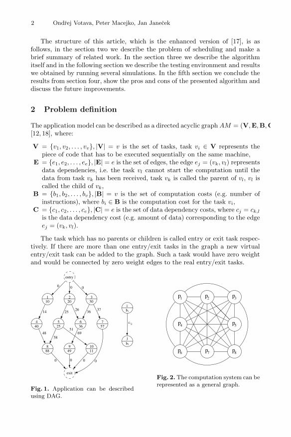
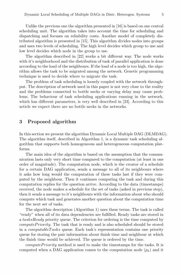
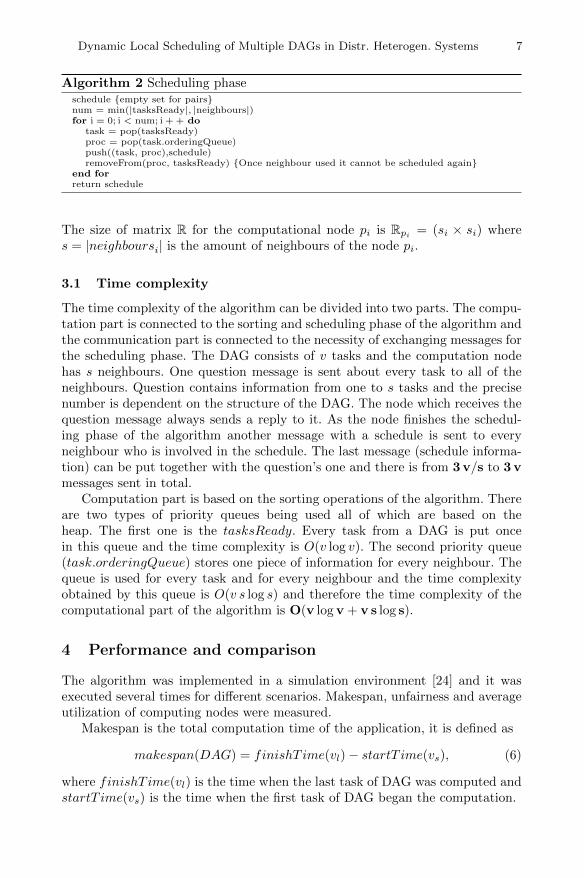
Fig. 3. Makespan for different numberof DAGs running concurrently (all plat-forms)

0

0.5

1

1.5

2

2.5

3

2 4 6 8 10

Ave

rage

unf

airn

ess

Number of DAGs


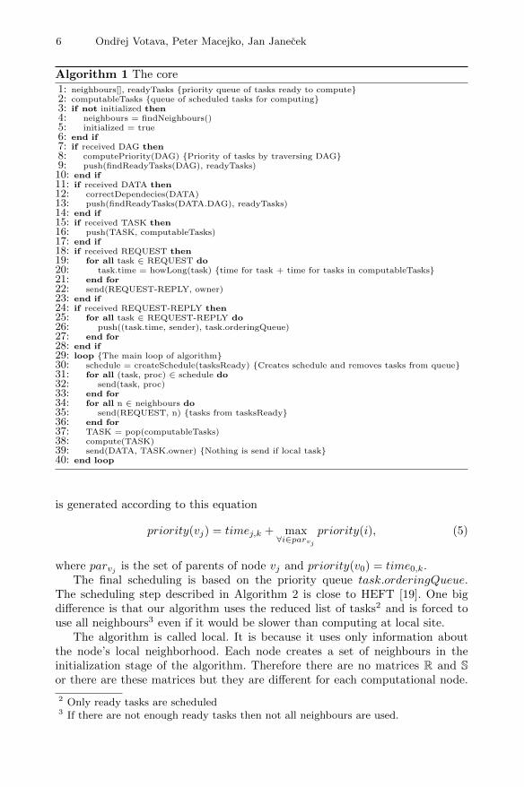
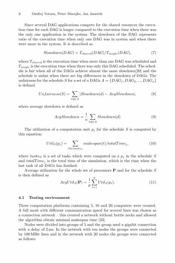
Fig. 4. Unfairness for different concur-rently running DAGs (all platforms)

– 4 groups of 5 nodes intraconnected by gigabit,– 2 groups connected by 100 MBit,– 3rd and 4th group connected by 10 MBit with others.

Sets of 2, 4, 6, 8 and 10 applications were generated using the method de-scribed in [19]. The application contained 25 tasks with different computationand data dependency costs. The schedule for each of the set was generated bysimulation4 of DLMDAG algorithm and by static algorithms HEFT and CPOP.

We used two methods of connecting several DAGs into one for the staticalgorithms, the first one is sequence execution of DAGs in a row, the secondone is to generate virtual start and end nodes and connect DAGs to these nodeswith a zero weighted edges. DAGs were ordered in the sequential execution testby the rule the shorter the makespan of DAG is the sooner it is executed. Intotal there were 100 sets of 2 DAGs, 100 sets of 4 DAGs etc. and the resultswe obtained we averaged. For the DLMDAG all DAGs arrived to the system attime 0 and on the one node.

4.2 Results

Results of sequential execution of DAGs for HEFT and CPOP achieved muchlonger makespans and therefore were not included into graphs. HEFT par andCPOP par mean that connection of DAGs was created using virtual start andend tasks.

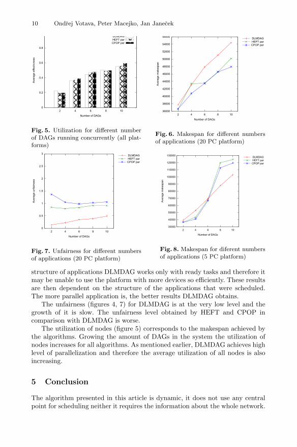
The makespan achieved by DLMDAG is very close to the HEFT and CPOP(fig. 3). The differences after averaging were just units of percents. The specialcase was the architecture of five computers (fig. 8), in this case DLMDAG out-performs the others. When there were 10 or 20 computers in the system (fig. 6),DLMDAG achieved slightly worse results. Since HEFT and CPOP use the whole

4 Simulation tool OMNeT++[24] was used


0

0.2

0.4

0.6

0.8

1

2 4 6 8 10

Ave

rage

effe

ctiv

ness

Number of DAGs


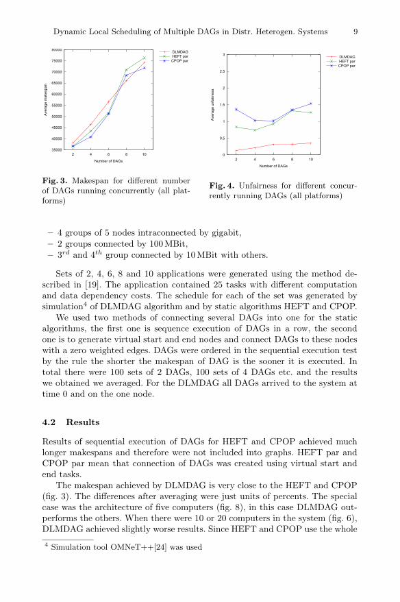
Fig. 5. Utilization for different numberof DAGs running concurrently (all plat-forms)

36000

38000

40000

42000

44000

46000

48000

50000

52000

54000

56000

2 4 6 8 10

Ave

rage

mak

espa

n

Number of DAGs


Fig. 6. Makespan for different numbersof applications (20 PC platform)

0

0.5

1

1.5

2

2.5

3

2 4 6 8 10

Ave

rage

unf

airn

ess

Number of DAGs


Fig. 7. Unfairness for different numbersof applications (20 PC platform)

30000

40000

50000

60000

70000

80000

90000

100000

110000

120000

130000

2 4 6 8 10

Ave

rage

mak

espa

n

Number of DAGs


Fig. 8. Makespan for diferent numbersof applications (5 PC platform)

structure of applications DLMDAG works only with ready tasks and therefore itmay be unable to use the platform with more devices so efficiently. These resultsare then dependent on the structure of the applications that were scheduled.The more parallel application is, the better results DLMDAG obtains.

The unfairness (figures 4, 7) for DLMDAG is at the very low level and thegrowth of it is slow. The unfairness level obtained by HEFT and CPOP incomparison with DLMDAG is worse.

The utilization of nodes (figure 5) corresponds to the makespan achieved bythe algorithms. Growing the amount of DAGs in the system the utilization ofnodes increases for all algorithms. As mentioned earlier, DLMDAG achieves highlevel of parallelization and therefore the average utilization of all nodes is alsoincreasing.

5 Conclusion

The algorithm presented in this article is dynamic, it does not use any centralpoint for scheduling neither it requires the information about the whole network.


DLMDAG is based on the local knowledge of the network – only neighbours cre-ate the schedule – and the schedule is created using several messages by which thecomputation times are gathered on the scheduling node. The simulations of thealgorithm were executed and results obtained were compared to the traditionaloffline scheduling algorithms.

DLMDAG is able to use the computation resources in a better way thancompared algorithms when there are more tasks in the system than computa-tion units. As the number of computation nodes increases the result DLMDAGachieves become worse than competitor’s.

Future work There are several possibilities to improve the proposed algorithm.Initially the computation systems do change. The algorithm should be able tomodify the schedules to reflect the network changes. Subsequently the currentalgorithm is fixed to the scheduling node and it’s neighbours and this may causeperformance problems, the algorithm could be able to move the application tosome other node with different neighbours.

References

1. D. Feitelson, L. Rudolph, U. Schwiegelshohn, K. Sevcik, and P. Wong, “Theory andpractice in parallel job scheduling,” in Job Scheduling Strategies for Parallel Pro-cessing (D. Feitelson and L. Rudolph, eds.), vol. 1291 of Lecture Notes in ComputerScience, pp. 1–34, Springer Berlin / Heidelberg, 1997. 10.1007/3-540-63574-2 14.

2. T. Hagras and J. Janecek, “A high performance, low complexity algorithm forcompile-time task scheduling in heterogeneous systems,” Parallel Computing,vol. 31, no. 7, pp. 653 – 670, 2005. Heterogeneous Computing.

3. H. Kikuchi, R. Kalia, A. Nakano, P. Vashishta, H. Iyetomi, S. Ogata, T. Kouno,F. Shimojo, K. Tsuruta, and S. Saini, “Collaborative simulation grid: Multiscalequantum-mechanical/classical atomistic simulations on distributed pc clusters inthe us and japan,” in Supercomputing, ACM/IEEE 2002 Conference, p. 63

4. D. Kehagias, M. Grivas, G. Pantziou, and M. Apostoli, “A wildly dynamic grid-like cluster utilizing idle time of common pc,” in Telecommunications in ModernSatellite, Cable and Broadcasting Services, 2007. TELSIKS 2007. 8th InternationalConference on, pp. 36 –39, sept. 2007.

5. A. Wakatani, “Parallel vq compression using pnn algorithm for pc grid system,”Telecommunication Systems, vol. 37, pp. 127–135, 2008.

6. M. Maheswaran, T. D. Braun, and H. J. Siegel, “Heterogeneous distributed com-puting,” in In Encyclopedia of Electrical and Electronics Engineering, pp. 679–690,John Wiley, 1999.

7. Y. kwong Kwok and I. Ahmad, “Benchmarking the task graph scheduling algo-rithms,” in In Proc. IPPS/SPDP, pp. 531–537, 1998.

8. J. Liou and M. Palis, “A comparison of general approaches to multiprocessorscheduling,” Parallel Processing Symposium, International, vol. 0, p. 152, 1997.

9. J. Ullman, “Np-complete scheduling problems,” Journal of Computer and SystemSciences, vol. 10, no. 3, pp. 384 – 393, 1975.

10. M. R. Garey and D. S. Johnson, Computers and Intractability: A Guide to theTheory of NP-Completeness. New York, NY, USA: W. H. Freeman & Co., 1979.


11. T. D. Braun, H. J. Siegel, N. Beck, L. L. Boloni, M. Maheswaran, A. I. Reuther,J. P. Robertson, M. D. Theys, B. Yao, D. Hensgen, and R. F. Freund, “A com-parison of eleven static heuristics for mapping a class of independent tasks ontoheterogeneous distributed computing systems,” Journal of Parallel and DistributedComputing, vol. 61, no. 6, pp. 810 – 837, 2001.

12. H. Topcuoglu, S. Hariri, and M. Wu, “Performance-effective and low-complexitytask scheduling for heterogeneous computing,” IEEE Transactions on Parallel andDistributed Systems, vol. 13, pp. 260–274, 2002.

13. M. Maheswaran, S. Ali, H. J. Siegel, D. Hensgen, and R. F. Freund, “Dynamicmatching and scheduling of a class of independent tasks onto heterogeneous com-puting systems,” Heterogeneous Computing Workshop, vol. 0, p. 30, 1999.

14. M. Iverson and F. Ozguner, “Dynamic, competitive scheduling of multiple dags ina distributed heterogeneous environment,” Heterogeneous Computing Workshop,vol. 0, p. 70, 1998.

15. M. A. Iverson and F. Ozguner, “Hierarchical, competitive scheduling of multipledags in a dynamic heterogeneous environment,” Distributed Systems Engineering,vol. 6, no. 3, p. 112, 1999.

16. X. Qin and H. Jiang, “Dynamic, reliability-driven scheduling of parallel real-timejobs in heterogeneous systems,” Parallel Processing, International Conference on,vol. 0, p. 0113, 2001.

17. O. Votava, P. Macejko, J. Kubr, and J. Janecek, “Dynamic Local Scheduling ofMultiple DAGs in a Distributed Heterogeneous Systems,” in Proceedings of the2011 International Conference on Telecommunication Systems Management, (Dal-las, TX), pp. 171–178, American Telecommunications Systems Management Asso-ciation Inc., 2011.

18. J. Janecek, P. Macejko, and T. M. G. Hagras, “Task scheduling for clustered hetero-geneous systems,” in IASTED International Conference - Parallel and DistributedComputing and Networks (PDCN 2009) (M. Hamza, ed.), pp. 115–120, February2009. ISBN: 978-0-88986-783-3, ISBN (CD): 978-0-88986-784-0.

19. H. Topcuoglu, S. Hariri, and M.-Y. Wu, “Task scheduling algorithms for hetero-geneous processors,” in Heterogeneous Computing Workshop, 1999. (HCW ’99)Proceedings. Eighth, pp. 3 –14, 1999.

20. H. Zhao and R. Sakellariou, “Scheduling multiple dags onto heterogeneous sys-tems,” Parallel and Distributed Processing Symposium, International, 2006.

21. J. Barbosa and B. Moreira, “Dynamic job scheduling on heterogeneous clusters,”in Parallel and Distributed Computing, 2009. ISPDC ’09. Eighth InternationalSymposium on, pp. 3 –10, 302009-july4 2009.

22. R. de Mello, J. Andrade Filho, L. Senger, and L. Yang, “Grid job schedulingusing route with genetic algorithm support,” Telecommunication Systems, vol. 38,pp. 147–160, 2008. 10.1007/s11235-008-9101-5.

23. Y. Kitatsuji, K. Yamazaki, H. Koide, M. Tsuru, and Y. Oie, “Influence of networkcharacteristics on application performance in a grid environment,” Telecommuni-cation Systems, vol. 30, pp. 99–121, 2005. 10.1007/s11235-005-4320-5.

24. A. Varga et al., “The omnet++ discrete event simulation system,” in Proceedingsof the European simulation multiconference (ESM’2001), vol. 9, p. 65, sn, 2001.

Documents

Dynamic Local Scheduling of Multiple DAGs in Distributed