Dynamic Line Rating for overhead lines – V6 documents/Regional_Groups... · Dynamic Line Rating ... design temperature of the line. Transmission line design ... DLR purposes is

ENTSO-E AISBL • Avenue de Cortenbergh 100 • 1000 Brussels • Belgium • Tel + 32 2 741 09 50 • Fax + 32 2 741 09 51 • [email protected] • www. entsoe.eu

Dynamic Line Rating for overhead lines – V6

CE TSOs current practice

RGCE SPD WG

30 March 2015



2

1. Contents

1. Contents ................................................................................................................................. 2

2. Introduction ............................................................................................................................ 3

3. Main Terminology ................................................................................................................... 3

4. The background and the aim of dynamic line rating (DLR) ..................................................... 4

Ampacity calculation of the line...................................................................................................................7

Algorithms for ampacity calculations ..........................................................................................................9

Information on atmospheric conditions ........................................................................................................9

5. Measuring system main features .......................................................................................... 10

6. Conductor Temperature Monitoring Methods ....................................................................... 11

6.1 Direct Monitoring Methods ..................................................................................................................11

6.2 Indirect Methods ...................................................................................................................................12

6.3 Method based on Wide Area Monitoring .............................................................................................13

6.4 Pro and Cons for Different Measurement Methods..............................................................................14

7. Approach .............................................................................................................................. 14

8. Main Applications ................................................................................................................. 14

9. Conclusion ........................................................................................................................... 17



3

2. Introduction

Based on the need to use more intensively the transmission system infrastructure TSOs have started to

investigate which measures are suitable in order to reach this goal. Furthermore for the TSOs construction of

new transmission lines is not a simple procedure, as a result of strictly environmental regulations. One of the

possible options identified to exploit the grid as much as possible is based on dynamic line rating by using

several available measurement and forecast techniques. The related data acquisition is very often combined

with meteorological measurements. By having both information available line conductor model can be

calibrated and used in a subsequent process in order to gain variable transmission line limits by using

environmental cooling or heating conditions as one major input factor. It should be noted that dynamic

thermal rating is not a substitute of grid development, but a complementary method to better exploit existing

infrastructures.

Implementation of the dynamic line rating is promising because it replaces the static rating. The static line

rating, evaluated with deterministic or probabilistic methods, is based on certain rather conventional

assumptions regarding atmospheric operating conditions. This approach had been widely accepted and used

decades ago when different direct and indirect measurements techniques were not available or were used very

seldom.

In last decade significant improvements in measurements and telecommunication has been made allowing

for testing dynamic line rating in real time operation. A quite significant number of TSOs approached to this

question in different ways and yet no final confirmation which combination of measurements and algorithms

represents an optimal solution is present.

The following report addesses only issues for overhead lines.

3. Main Terminology

Thermal current limit (current carrying capacity / ampacity) is defined as the maximum amount of

electrical current a conductor or device can carry before sustaining immediate or progressive deterioration.

Static thermal current

A static thermal current is a current which causes that conductor, operating under presumed atmospheric

conditions, designed for certain maximum continous operating temperature and certain maximum operating

sag, reaches one of either limits: the maximum conductor temperature or the maximum sag.

Since constant atmospheric conditions may only be established in controlled laboratory conditions also

steady-stae thermal current confirmation is limited to such environment and usually does not include all

detailed mechanical behaviour of the entire line.

Dynamic thermal current

A dynamic thermal current is a current which causes that conductor, operating under real atmospheric

conditions, designed for certain maximum continous operating temperature and certain maximum operating

sag, reaches one of either limits: the maximum conductor temperature or the maximum sag.

Since real atmospheric conditions vary greatly even in “stable atmospheric conditions” the dynamic thermal

current also varies accordingly. Dynamic thermal current may be determined in special test facilities where

the conductor’s temperature is controlled with closed-loop regulation of a current source.

Current carrying capacity of conductor

Current carrying capacity of a conductor is defined for a certain construction and implies certain ambient

conditions and is usually provided by the manufacturer of the conductor. Current carrying capacity is

therefore related to material and construction of the conductor at given ambient conditions. It should be



4

noted that mechanical implementation of a certain conductor may result in lower current carrying capacities

then those from sepcifications because of lower maximum design temperature of the line.

Transmission line design temperature

Transmission line design temperature is a maximum temperature that conductor in any span may reach

without any fear that the safety clearances will be violated. It should be noted that design temperature may

be lower than the maximum temperature of finished (stranded) conductor may reach.

4. The background and the aim of dynamic line rating (DLR)

The aim of dynamic line rating is to safely utilise existing transmission lines transmission capacity based on

real conditions in which power lines operate. A crucial difference between static and dynamic line rating is

that “static current” is calculated based on rather conventional atmospheric conditions while dynamic line

rating takes into account actual atmospheric conditions which most of the time offer better cooling and thus

allow higher “dynamic” current, contributing to improve safety.

Calculating the dynamic line rating of an overhead transmission line is a demanding task because it must

inherently solve two problems:

1. determination of the thermal current limit1 for a particular span which may involve different

measurements and different calculation techniques,

2. determination of the weakest span i.e. the span which represents a limit for the whole power line,

which presumes that determination of thermal current for all spans has been performed;

furthermore the weakest span may vary in consequence of different atmospheric conditions and

span characteristics (tension, clearance margin, etc...).

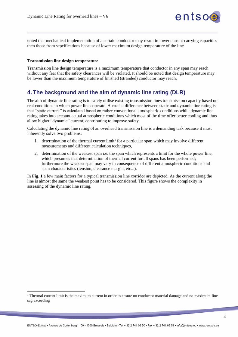
In Fig. 1 a few main factors for a typical transmission line corridor are depicted. As the current along the

line is almost the same the weakest point has to be considered. This figure shows the complexity in

assessing of the dynamic line rating.

1 Thermal current limit is the maximum current in order to ensure no conductor material damage and no maximum line

sag exceeding



5

h

Tamb

-

v

Si

Tcond

I line

current

due to the high solar

radiation and low

wind the conductor

reaches highest

temperatue

ambiental

temperature

high wind at the ridge

highest solar

radiation

I/Imax

temperature profile of

the conductor

100% 92%

64%53%

43%56%

span current

limit

weakest span with

lowest thermal limit

low wind in the valey

Figure 1: The variability of influencing factors on transmission line rating

As seen from Figure 1 the current carrying capacity of a span is influenced by the atmospheric conditions.

If we assume that conductor is mechanically properly designed and the sag is not a limiting factor for

temperatures below the maximum allowable permanent temperature of the conductor, then the weather

conditions have the dominant effect on line’s ampacity. The weather conditions directly influence on

cooling power - mainly through convective cooling provided by wind. The approximate differential

equation that describes the change of conductor temperature is as follows:

cpmdT

dt= pjoul + psol + pmag − pcon − pcon − prad (1)

where are:

pjoul joule heating

pmag magnetic heating

pjoul solar heating



6

pcon convective cooling

prad radiative cooling.

This equation is telling us that when the heating is greater than cooling, the temperature will rise

proportionally to the mass and specific heat of the conductor and vice versa. Since the atmospheric

conditions around the conductor constantly vary as well as the conductor load, the temperature of the

conductor also varies accordingly.

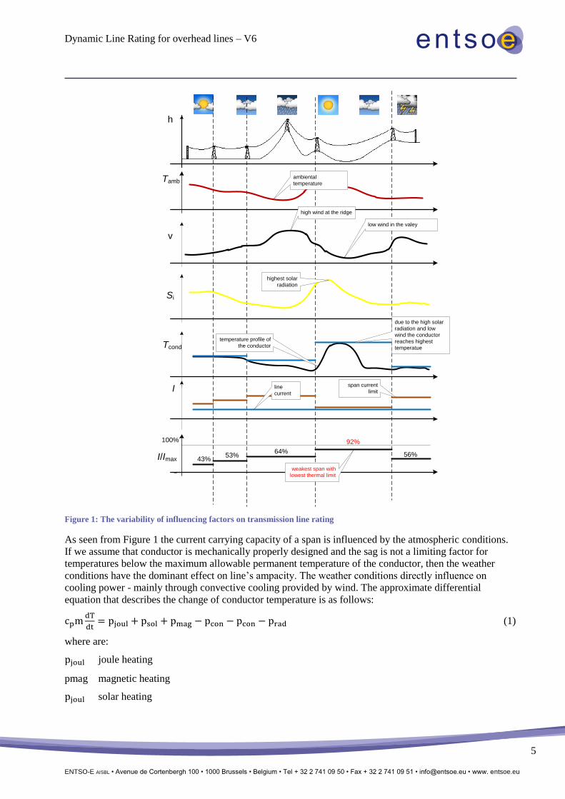
Figure 2 shows an example of the variability of the conductor temperature in 6 hours time span. What can

be learnt from the figure is that the main impact comes of course from the line current, but also that weather

conditions have a significant impact. Finally the more operational limits are reached the complex model-

based approaches might be in order to correctly reflect the real behaviour. In the case of the shown example

one circuit of a double line path was opened due to a fault (red line). The second circuit have reached a line

current exceeding 2000 A (blue line). The green and cyan curves shows the direct measured conductor

temperature on two different locations while the blue light and orange curves represent the corresponding

outside ambient temperature.

Figure 2: Conductor temperature and line current measurements alongalong 6 hours

It should be noted that solving differential equation 1 for the temperature does not mean that DLR problem

is solved. Knowing the temperature of the conductor is of significant importance for assessment purposes,

but the real question is, which is the allowed current that would not breach the maximum allowed

temperature of the conductor? The TSO operating the grid needs to know, which is the maximum ampacity

or allowed load of the line, not what is the temperature of the line. The temperature is merely the result of

-10

0

10

20

30

40

50

60

70

0

500

1000

1500

2000

2500

3000

06

:00

06

:15

06

:30

06

:45

07

:00

07

:15

07

:30

07

:45

08

:00

08

:15

08

:30

08

:45

09

:00

09

:15

09

:30

09

:45

10

:00

10

:15

10

:30

10

:45

11

:00

11

:15

11

:30

11

:45

12

:00

12

:15

12

:30

12

:45

[°]

[A]

F_L_Rob2_LaPu.i.ps.scal.abs F_L_Rob1_Sils.i.ps.scal.abs dT_Preda_LaPunt dT_Preda_Lagalb dT_Albula_LaPunt dT_Albula_Lagalb



7

certain operating condition (load and atmospheric conditions), the real cause is the current that through the

Joule losses heats the conductor.

For understanding what are the differences between the ampacities at different atmospheric conditions one

should look at the Figure 3. It shows needed current change at different atmospheric conditions for a certain

conductor to increase the initial conductor temperature from 50 °C and to maximum conductor temperature

which is 80 °C. With other words; if line current results, under certain atmospheric conditions, in 50 °C

temperature of the conductor, what is the increase of the current that would produce the conductor

temperature of 80 °C under the same conditions?

Figure 3: Steady-state current needed to heat the conductor to 50 and 80 °C in different ambient conditions

As can be seen from Figure 3 the needed current change varies with ambient temperature and effective wind

speed quite nonlinearly. Higher temperatures and wind speeds require higher current change to reach 80 °C,

which means that under these conditions according to the model used, reserve in ampacity is surprisingly

higher than in low temperature and low wind conditions.

The illustration from Figure 3 has important message about utilization of the temperature monitoring in

DLR. The main conclusion is that only temperature monitoring for DLR purposes is not enough as line

loading and atmospheric conditions are completely uncorrelated. The same temperature of the conductor

may be reached with low load in hot ambient and low wind or with high load in low ambient temperature

and high wind. For DLR which results in ampacity of the line the atmospheric condition must be included

as they define cooling conditions of the conductor.

Ampacity calculation of the line

The ampacity calculation of the line may be performed by utilization of different techniques and

algorithms. If we stick with the initial ideal requirement that DLR should be performed for the full length of

the line then the required items for ampacity calculation are as follows:

1. algorithm for ampacity calculation.



8

2. input data:

a. physical properties of the conductor,

b. geographical information for all spans,

c. atmospheric conditions for all spans, in order to be aware of hot spots like spans with low

clearance or reduced conductor cross-section

Once all required data are in place the calculation of ampacities of all spans of the line may be calculated.

The lowest ampacity of all the spans is the bottle-neck of the line and it represents the current ampacity of

the line as can be seen from Figure 4.

Figure 4: Practical example of ampacity determination for every span

Once such system is established the dynamic line rating data may be analysed for a certain time period.

Results may be used for developing risk mitigation strategies. Depending on several factors that tailor line’s

ampacity like line design temperature, conductor properties, atmospheric conditions, etc. a very important

role has also the algorithm used in the ampacity calculations. One should be aware that each influencing

factor introduces certain uncertainties into the ampacity determination. We should point out that in general

the uncertainty of every input data must be known in order to be able assessing the uncertainty of final

result – the ampacity of the line. This task is very demanding and needs a lot of theoretical and

experimental work which to some extent is yet to be done.

The ampacity calculation by DLR should properly take into account the possible mechanical behaviour of

the conductor at high temperature or in presence of great step of temperature change, especially when this

technicque is applied to old lines: in fact the mechanical characteristics of stressed joints and other

mechanical components can determine conductor break.

Figure 5 illustrates one of the possible ways how to deal with dynamic line rating by defining a variable time

depending area in which crossing of dynamic line limit and static line limit compels to use lower limits, in

order to maintain adequate security conditions.



9

t [h]8760

Ith_stat

Very important question Ith_dyn < Ith_stat?

current limit – static rating

Legend:

dynamic current limit

static current limit

duration Ith_dyn < Ith_stat

Legend:

dynamic current limit

static current limit

duration Ith_dyn < Ith_stat

current limit - dynamic line rating

Ith

Figure 5: Comparison of static and dynamic current limits

Algorithms for ampacity calculations

different algorithms exist which allow for calculation of the ampacity of the particular span or tensioning

section. Most known are CIGRE and IEEE. These two algorithms are widely used either in original form or

they are tailored to specific implementation philosophy at a TSO like linearization or other changes.

It should be emphasized that ampacity calculation algorithms inherently include certain mathematical

model of heating and cooling of the conductor. As such, they are prone to errors and they introduce

uncertainties which may be substantial especially when the loading of the line is approaching maximum

conductor temperature e.g. 80 °C. For this reason, we see that future work in DLR domain should be

focused on improvements of the ampacity calculation algorithms for which should be also known the

uncertainties. This approach will help DLR systems to be considered serious systems not just “pilot

projects”

Information on atmospheric conditions

Atmospheric conditions are another crucial data set needed for ampacity calculation. It is obvious that

atmospheric conditions vary along the line and thus have predominant influence on heating/cooling balance

of the conductor. Ideally we should have measured atmospheric conditions in every span, but such system

would be to simply too expensive.

There are several possible solutions to this problem. However the main idea is to use established renown

weather services for measurements, modelling, processing and data providing. The key reason for this

approach is that weather services providing data sets for direct or indirect use in thermal rating have dedicated

personnel, hardware, software and internal processes that provide data with certain quality. This allows to

establish SLA (service level agreement) based contract for weather data delivery.



10

Ambient measurements

Optional conductor meas.

temperature

tension

sag

temperature wind solar radiation

Digital surface model

Ambient conditions per

span

Mesoscale or other weather

model results

Geographical infromation

about the line and spans

Phyisical properties of

conductor

Microscale weather

calculation

Dynamic line rating

calculation

Ampacity result

Maximal timeLoad of the line

SCADA

Figure 6: Possible imeplementation of different weather data sources for calculation of ampacity

5. Measuring system main features

It should be noted that DLR monitoring equipment can be installed somewhere (single or multiple

locations) on or along the monitored line. Since a single transmission line may be several tens or even

hundreds of kilometres long, and may pass different kinds of terrain, geographical locations, vegetation and

varying weather circumstances along the line, the choice of monitoring device locations is of primary

importance. The selected location(s) for the DLR monitoring systems should be the most critical location(s)

along the transmission line, so that if the line is secure in this section then it is secure also anywhere along

the line itself. However, the exact definition of those locations is quite challenging and depending on local

weather conditions.

As for dynamic line rating exact and tailored measuring systems are of crucial importance and their

characteristics have to be considered in detail. The related systems shall have the following features:

• Accuracy: the system must be able to provide rating estimates with the lowest possible error.



11

• Precision: the system must be able to assess the error associated with the estimate given and this error

should be reduced as much as possible.

• Reliability: the system must be able to provide real-time data also in case of measurement or

communication failures, reducing gradually its performance.

• Spatial resolution: the system must be able to provide estimates with a spatial resolution sufficient for

the identification of hot spots. Overhead lines can be extended over long distances and different

environmental conditions. Therefore, the rating of the conductor will change along the path and it is

necessary not to exceed the rating of the most constrained component.

• Temporal resolution: the system must be able to provide estimates within an acceptable time limit, in

order to prevent the insurgence of potentially dangerous situations created by reduced component

thermal capacitance, environmental conditions variability and electric power transfer variability. As

shown in Figure 2 a drastic temperature rise took place within a few minutes.

• Cost effectiveness and ease of deployment and maintenance: the cost of the system must be justified

by the economical return in terms of enhanced network reliability or power transfer capability.

6. Conductor Temperature Monitoring Methods

Conductor temperature of overhead power lines can be monitored through direct and indirect methods. The

first are based on the measurement of the conductor temperature or least one physical parameter of the line

which is directly related to it, such as sag, mechanical tension, vibration frequency, line angle of catenary, or

ground clearance.

The indirect methods use weather parameters, measured by meteorological stations, and the conductor

electrical load to calculate the temperature of the conductor, through theoretical models.

6.1 Direct Monitoring Methods

The direct methods are based on monitoring several parameters of a power line:

Conductor temperature measurement

The method that employs the direct temperature measurement requires the installation of devices on the

conductor, which can also be powered by the magnetic field generated by the line current.

The conductor temperature can be measured through:

• Temperature sensors: direct temperature measurement is usually performed by temperature sensors,

which transmit the measurements via radio communication to a central station or need to be locally

downloaded. These sensors are located on a few positions only: they measure the conductor surface

temperature and not the average conductor temperature of the span where they are installed. So the

conversion from this measured temperature to the corresponding sag is necessary to estimate the

conductor position in real-time. Should be noted that the direct or close contact of the temperature sensor

with an energized conductor can cause some side effects: mechanical (abrasions, sensor-conductor

shock, vibrations, breaks), chemical (oxidations, galvanic activity), dielectric and electromagnetic (eddy

currents), thermal (self-heating).



12

• Infrared thermal camera: the infrared radiation from the conductor is used to determine its temperature,

using an IR detector. The sensor can be mounted remote from the conductor, i.e. on the transmission

tower, and therefore do not require high voltage insulation. Additionally, it may not be necessary to

outage the line during installation or maintenance.

• Optical fibre (Distributed Temperature Measurements): the temperature measurement through optical

cables, Distributed Temperature Measurements (DTM), is carried out by the analysis of the phenomenon

of scattering produced by a correct laser beam sent into the optical fibre. The analysis of these signals

provides information on the temperature distribution along the optical fibre for distances up to more than

20 km, with a spatial resolution that can reach a few meters.

Line tension methods

The methods involving the measurement of the mechanical tension of the line (Line tension methods) use

load cells installed on selected pylons of the line, which measure the mechanical tension and transmit the

information to the control centre. Here data is used for the calculation of temperature and therefore of the

real-time ampacity.

Line sag methods

The methods that employ the measurement of the sag (Line sag methods) rely optical sensors, ultrasonic or

radar to measure the sag (or the clearance to ground) in fixed spans of the line.

Vibration frequency

Power line conductors always move due to wind conditions: indeed wind turbulence as well as wind spatial

coherence along the span, easily generate small (or large) movements that include the intrinsic mechanical

oscillation frequencies of the span.

The analysis of the conductor vibration can be used to detect the fundamental frequency of the span, which

is a function solely of the sag.

A device is attached directly to the overhead power line conductor and it is able to evaluate the sag of a span

in real-time, without knowing any data.

Line angle of catenary

Angle measurement devices use the conductor angle to calculate the actual conductor sag. Indeed a parabola

shape (or even better a cosh), which identifies the catenary, can be rebuild based on the knowledge of the

slope of the parabola at a given point of the curve (to be known), if the span length and some conductor data

are known.

6.2 Indirect Methods

Indirect methods require the installation of meteorological stations in one or more points along the line:

usually weather sensors are directly installed on the pylons of the line. The line conductor is simulated by a

mathematical model which, starting from meteorological data and the values of line current acquired in real

time, calculates the temperature of the conductors themselves and performs a forecast of overload capability

for fixed periods.

Meteorological parameters to detect are the speed and direction of the wind, the ambient temperature and the

solar radiation. The wind speed is the most important factor in determining the temperature of the conductor,

so particular attention should be placed in its detection: anemometers used must be capable of measuring,

with good accuracy, wind speeds even lower than 1 m/s (ultrasonic anemometers provide definitely the best

performance).

By using this method the confindence in correct modelling should be quite high, no calibration is possible

and the impact of emissivity and reflectivity should not be underestimated.



13

6.3 Method based on Wide Area Monitoring

As seen, the temperature estimation may be obtained through a:

• Direct measurement of the sag and temperature: nevertheless, this method is suitable for the estimation

on a single critical span rather than on an entire line.

• Thermal model of the line, based on weather conditions knowledge: however, weather conditions may

significantly vary along the line, especially for long connections, so that this method not always allows

an accurate estimation.

To overcome the limitations of these two methods, it is possible to use another method based on WAMS

(Wide Area Measurement System) measurements. In particular, this technique consists in the real-time

reconstruction of the electrical parameters of the line based on the elaboration of the WAMS measurements.

Comparing the real-time values with the standard values is possible to estimate with a good accuracy the

current temperature of the line thus consider a mean value along the whole length. However, if the line is

crossing a region with e.g. significant changes with respect to altitude the corresponding cooling impact will

have to be considered.

Figure 7: WAM DLR approach

The estimation of the line’s temperature is based on the identification of the electrical parameters of the line

itself. These parameters may be calculated from the electrical measures (WAMS data) of the line through an

adequate electrical model.

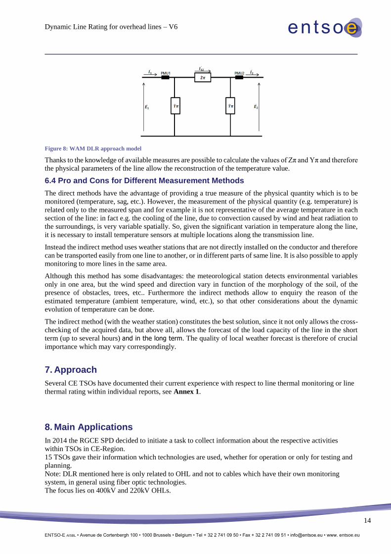
Figure below shows a scheme of the model adopted (Π model of the line). With E1, I1, E2 and I2 are indicated

the available measures, namely voltage and current phasors provided from PMUs (Phasor Measurement

Units) located at the ends of the line. Zπ and Yπ are the equivalent series impedance and shunt admittance

while I12 indicates the average current of the line.



14

Figure 8: WAM DLR approach model

Thanks to the knowledge of available measures are possible to calculate the values of Zπ and Yπ and therefore

the physical parameters of the line allow the reconstruction of the temperature value.

6.4 Pro and Cons for Different Measurement Methods

The direct methods have the advantage of providing a true measure of the physical quantity which is to be

monitored (temperature, sag, etc.). However, the measurement of the physical quantity (e.g. temperature) is

related only to the measured span and for example it is not representative of the average temperature in each

section of the line: in fact e.g. the cooling of the line, due to convection caused by wind and heat radiation to

the surroundings, is very variable spatially. So, given the significant variation in temperature along the line,

it is necessary to install temperature sensors at multiple locations along the transmission line.

Instead the indirect method uses weather stations that are not directly installed on the conductor and therefore

can be transported easily from one line to another, or in different parts of same line. It is also possible to apply

monitoring to more lines in the same area.

Although this method has some disadvantages: the meteorological station detects environmental variables

only in one area, but the wind speed and direction vary in function of the morphology of the soil, of the

presence of obstacles, trees, etc.. Furthermore the indirect methods allow to enquiry the reason of the

estimated temperature (ambient temperature, wind, etc.), so that other considerations about the dynamic

evolution of temperature can be done.

The indirect method (with the weather station) constitutes the best solution, since it not only allows the cross-

checking of the acquired data, but above all, allows the forecast of the load capacity of the line in the short

term (up to several hours) and in the long term. The quality of local weather forecast is therefore of crucial

importance which may vary correspondingly.

7. Approach

Several CE TSOs have documented their current experience with respect to line thermal monitoring or line

thermal rating within individual reports, see Annex 1.

8. Main Applications

In 2014 the RGCE SPD decided to initiate a task to collect information about the respective activities

within TSOs in CE-Region.

15 TSOs gave their information which technologies are used, whether for operation or only for testing and

planning.

Note: DLR mentioned here is only related to OHL and not to cables which have their own monitoring

system, in general using fiber optic technologies.

The focus lies on 400kV and 220kV OHLs.



15

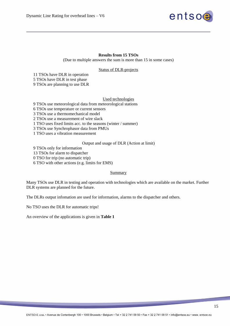
Results from 15 TSOs

(Due to multiple answers the sum is more than 15 in some cases)

Status of DLR-projects

11 TSOs have DLR in operation

5 TSOs have DLR in test phase

9 TSOs are planning to use DLR

Used technologies

9 TSOs use meteorological data from meteorological stations

6 TSOs use temperature or current sensors

3 TSOs use a thermomechanical model

2 TSOs use a measurement of wire slack

1 TSO uses fixed limits acc. to the seasons (winter / summer)

3 TSOs use Synchrophasor data from PMUs

1 TSO uses a vibration measurement

Output and usage of DLR (Action at limit)

9 TSOs only for information

13 TSOs for alarm to dispatcher

0 TSO for trip (no automatic trip)

6 TSO with other actions (e.g. limits for EMS)

Summary

Many TSOs use DLR in testing and operation with technologies which are available on the market. Further

DLR systems are planned for the future.

The DLRs output infomation are used for information, alarms to the dispatcher and others.

No TSO uses the DLR for automatic trips!

An overview of the applications is given in Table 1



16

Table 1: Current TSOs DLR applications overview

Croatia HOPS 110 25km XIn Use: Temperature and current sensors directly at the conductor of the

OHL´s; Central evaluation of dataOTLM X

Croatia HOPS 400kV 61kmLine Thermal Monitoring application - use of synchrophasor data on line

terminalsABB PSGuard X

Croatia HOPS 400/220kV XLine Thermal Monitoring application - review of approach of using

synchrophasor dataX

Denmark energinet.dk 400 0% 0% 0%

Denmark energinet.dk 220 0% 0% 0%

Denmark energinet.dk 150 0% 0% 20% Technology not decided Yes

Used in

operational

planning

Germany TenneT 400/220kV4700km

= app. 50%X

In Use: Meteorological data from own meteorological stations (ambient

temperature, wind speed) within 40 different climate zonesX

Germany TenneT 400/220kV X Reviewing the approach: Measurement of the wire slack NEXANS X

Germany TenneT 400/220kV X Reviewing the approach Temperature sensors MICCA X

Germany transnetBW 400kV x Fixed limits acc. to season (winter or summer) X

Germany Amprion 400kV X X X "CIGRE" thermal model X

Hungary MAVIR 400 kV XReviewing the approach: Measurement of the wire slack or/and

Temperature sensorsX

Information for

the market

Italy TERNA 400kV 8 OHL 10 OHL X XTemperature Sensors directly at the conductor. Thermo-mechanical model

using weather conditions near to the lineMicca

To

maintena

nce and

Engineeri

ng Dept.

Limits for EMS

System

Italy TERNA 220kV 1 OHL XTemperature Sensors directly at the conductor. Thermo-mechanical model

using weather conditions near to the lineUSI

To

maintena

nce and

Engineeri

ng Dept.

Limits for EMS

System

Italy TERNA 150 kV 2 OHL 1 OHL X XTemperature Sensors directly at the conductor. Thermo-mechanical model

using weather conditions near to the lineMicca/USI

To

maintena

nce and

Engineeri

ng Dept.

Limits for EMS

System

Poland PSE 400/220kV 100% X

Meteorological data supplied by national institut of meteorology from

meteorological stations (ambient temperature) at over 200 sites in the

country.

Calculation of limits based upon sag-checking.

EPRI/Siemen

sX

Limits for EMS

System

Slovenia ELES 400 1 (10%) X X

Reviewing the approach: mezo scale meteorological data + micro scale

atmospheric dynamics calculation + low definition ambient conditions

measurements + DTR algorithm EIMVX

Slovenia ELES 400 3 (30%) X X X

Planned approach for line category I: mezo scale meteorological data +

micro scale atmospheric dynamics calculation + high definition ambient

conditions measurements + DTR algorithm TenderX


Planned approach for line category II: mezo scale meteorological data +


conditions measurements + DTR algorithm TenderX

Slovenia ELES 400 60 (60%) XPlanned approach for line category III: mezo scale meteorological data +

DTR algorithm Tender X

Slovenia ELES 220 1 (14%) XReviewing the approach: low definition ambient conditions measurements

+ DTR algorithmARTES X

Slovenia ELES 220 2 (28%) x x


atmospheric dynamics calculation + low definition ambient conditions

measuremnts + DTR algorithm

EIMV X

Slovenia ELES 220 2 Reviewing the approach: Conductor temperature measurement at one point OTLM X

Slovenia ELES 220 5 (71%)

X X X

Planned approach for line category I: mezo scale meteorological data +


conditions measurements + DTR algorithm

Teneder X



Slovenia ELES 110 1 xReviewing the approach: Longitudinal conductor temperature measurement

+ ambient conditions measurements + DTR softwareNKT X X

Slovenia ELES 110 2 Reviewing the approach: Conductor temperature measurement at one point OTLM X

Slovenia ELES 110 1 X X


atmospheric dynamics calculation + high definition ambient conditions

measurements + DTR algorithm

EIMV X


Planned approach for line category II: mezo scale meteorological data +


conditions measurements + DTR algorithm Tender X



Spain REE 220

30 km

overhead line

María -

Fuendetodos 1

Evaluation

7 own

weather

stations at 10

m high

DTS temperature measurements 30 km NKT

Wind power

production

integration

Switzerland Swissgrid 380 4 6 x diff. technologies including WAM LTM CAT-1, micca X

Switzerland Swissgrid 220 2 2 x & Webcams for icing control R&D micca R&D

ELES: * all percenatge values are related to number not length of the line



17

9. Conclusion

Based on collected data and field experiences from ENTSO-E members the following conclusions may be

drawn:

1. Many OHLs within the 400 and 220 kV ENTSOE-Grid are more and more heavily loaded due to

increased power flow caused by far located renewable sources or cross border trading.

2. Today the maximum capacities of OHLs are typically calculated in a conventional way under worst

case assumptions like maximum ambient temperature and no wind. Therefore under normal

conditions there are presumably free capacities on the OHLs which are not used today – especially

during windy days and in windy regions. However, a few TSOs have already introduced fix

seasonal thermal limits which already ensure a corresponding flexible operation.

3. The aim of dynamic line rating (DLR) is to safely utilise existing transmission lines transmission

capacity based on real conditions in which power line operates. There are two key advantages

expected from DLR: increase of the capacity and improved safety of operation.

4. Dynamic thermal rating is not a substitute of grid development, but a complementary method to

better exploit existing infrastructures.

5. In some countries the maximum design temperature of the lines built 30-40 years ago is lower than

80 °C. This fact may additionaly contribute to introduce DLR. Some countries undertook redesign

of the OHL to meet safety clearances.

6. Since some years there are different monitoring technologies on the market or under development

which are designed to measure certain line parameters like conductor temperature, tension or sag.

These mesurements may be useful when calculating the line ratings however they are not sufficient

for DLR.

7. DLR must take into account atmospeheric conditions because lower ambient temperatures and

higher wind speeds improve conductor cooling.

8. Calcualtion of ampacity for the full line length is very demanding, because information on

atmospheric conditions with known uncertainty for each span must be know.

9. Beside uncertainties of the atmospheric conditions also uncertainty of the algorithm used in

calculation must be known. Since power lines usualy do not operate at maximum design

temperatures, corresponding filed results are not available and uncertainities can not be established

unless dedicated test polygons are used.

10. It must be admitted that without knowing the uncertainties of the atmospheric conditions and

algorithms and without being able to confirm relevancy of the DLR results in real-time operation,

since marginal operating conditions are not present, any judgement about average or maximum

increased capacity may be misleding or even false.

11. It should be noted also that under certain conditions the DLR may push the thermal loading beyond

the stability limit (in particular transient, voltage or small signal stability) or introduce too high

reactive power losses for which the necessary reactive compensation may not be available. These

issues have to be carefully considered before the additional loadability is made available.

12. Compared to the current rigid approach DLR may allow an increase in loading but we have to

reserve a margin for the uncertainties associated with the applied method. An accurate assessment

of this margin requires detailed analysis based on pilot installations over long time periods.

Documents

Dynamic Line Rating for overhead lines – V6 documents/Regional_Groups... · Dynamic Line Rating ... design temperature of the line. Transmission line design ... DLR purposes is