Dynamic Leadtime Management in Supply Chains

Alp Muharremoglu ∗ John N. Tsitsiklis†

June 2003

∗Graduate School of Business, Columbia University, New York, NY, 10027; e-mail: alp2101@columbia.edu†Laboratory for Information and Decision Systems and Operations Research Center, M.I.T, Cambridge, MA,

02139; e-mail: jnt@mit.edu

Abstract

One way to hedge against random fluctuations of demand in supply chains is to keep inventories at

various points in the chain. Another is to actually modify the leadtimes in the system dynamically.

Working with multiple suppliers, using multiple transportation options, having the option to

expedite certain processes, or having different possible routes for a unit to go through the supply

chain are all examples of having flexibility in the supply chain leadtimes. In this paper, we

study a serial inventory system with complete leadtime flexibility. For expositional purposes,

we use a terminology that corresponds to making shipment (routing) decisions in the supply

chain, however, the model can represent many different types of leadtime flexibility, such as the

ones described above. In particular, we allow the option of shipping units from any stage in the

supply chain to any downstream stage. This option gives the manager an additional flexibility

that can be utilized as the uncertain demand is revealed. The shipments incur origin-destination

dependent costs. Under a certain supermodularity assumption on the shipment costs, we show

that optimal policies can be characterized as extended echelon base stock policies, which is a

natural generalization of the well known echelon base stock policies.

1 Introduction

One way to hedge against random fluctuations of demand in supply chains is to keep inventories

at various points in the chain. Accordingly, there is a large body of academic work on the subject

of multi-echelon inventory management. Most of this literature assumes that leadtimes in the

supply chain are exogenously determined. However, another widely used method for responding

to demand fluctuations is to actually change the leadtimes in the system dynamically. Working

with multiple suppliers, using multiple transportation options, having the option to expedite

certain processes, or having different possible routes for a unit to go through the supply chain

are all examples of having flexibility in supply chain leadtimes. For example, consider a supply

chain where products typically go through a national warehouse, a regional warehouse, and are

then sold to end customers by a retailer. If at some point the inventory level at the retailer

gets dangerously low due to an unexpected rise in demand, the manager at the retailer may

want to place an order at the national warehouse directly, bypassing the regional warehouse.

This may be a faster and worthwhile way of replenishing inventory, albeit possibly at a higher

cost. Another common situation is one involving alternative transportation options. For example,

Hewlett Packard’s Network Server Division manufactures a major subassembly of network servers

in Singapore and ships it to its distribution centers, where the assembly is completed due to

customer specifications. Two modes of transportation with different leadtimes and costs are

available (air and ocean) between the factory and the distribution centers (See Beyer & Ward

2001). Both of these examples involve dynamically modifying the leadtimes in the supply chain, in

response to demand fluctuations. This paper investigates optimal policies for such multi-echelon

systems, where inventories and leadtimes are managed simultaneously.

In addition to supply chains, this model may be applicable in a manufacturing setting as

well. Suppose that as part of a manufacturing operation, a product needs to go through sev-

eral processes sequentially, and that there is both work in process inventory as well as finished

goods inventory in the system. At certain points of the manufacturing process, there may be the

possibility to speed up certain processes, by renting additional machines, hiring temporary em-

ployees, reprioritizing, or outsourcing. Such situations can be modeled as one involving dynamic

management of leadtimes, and can be handled using the model in this paper.

In order to make the exposition clear, while developing the results, we use a terminology that

corresponds to a particular type of leadtime flexibility. In particular, we consider the question of

managing a multi-echelon inventory system, where units do not have to go through the supply

chain over a predetermined path, and shipping (or routing) decisions are made in a dynamic

fashion. However, the results that we obtain at the end are applicable to settings with other types

of leadtime flexibility as well, such as systems with multiple suppliers or alternative transportation

options. Section 6.2 includes a discussion on such alternative interpretations.

1

We analyze a multi-echelon inventory system with complete flexibility in the way a unit goes

through the stages in the system. Consider the classical serial inventory system of Clark & Scarf

(1960). In this system, units go through a series of inventory stages, until they are ready to satisfy

customer demand. Every unit goes through all the stages in the same sequence. Shipment from a

stage to the next one has a certain cost rate associated with it. In this paper, we present a model

where units do not have to go through all the stages of the system, and can be transferred from

any stage to any downstream stage, by incurring a certain cost, that depends on both the origin

and the destination of the unit. This option gives the controller an additional flexibility that can

be utilized as the uncertain demand is revealed. The queueing analogy is that the classical serial

inventory system of Clark & Scarf (1960) corresponds to a tandem queueing network, whereas

the inventory system studied in this paper corresponds to a feed-forward network of queues.

The paper that is most closely related to our work is Lawson & Porteus (2000). Our model

effectively generalizes the one studied by Lawson & Porteus (2000), by allowing a more general cost

structure. The term dynamic leadtime management was used in that paper to reflect flexibility

in the system leadtime, that is, the time it takes for a unit to go through all the stages in a

serial system. Their model is closely related to ours, even though it is presented in a somewhat

different manner. Similar to our model, they consider a serial system. But in their model, the

units have to go through all the stages. They allow the transition from a stage to another to

be expedited, making it essentially instantaneous. Since a unit can be expedited through several

stages within the same period, such a transition can also be viewed as transferring the unit from

a stage to another by skipping others in between, just like in our model. The main difference is

that Lawson & Porteus (2000) use an additive cost structure, meaning that the cost of expediting

through several stages is equal to the sum of the one-step expediting costs. Our model assumes

a more general, “supermodular” cost structure, which includes the special case of additive costs.

(See Section 4 for details). In fact, it is general enough to include every cost structure where the

cost of a shipment is a convex function of the number of stages that the unit bypasses.

The main contribution of this paper is a characterization of optimal policies for this multi-

echelon inventory system. These optimal policies have different interpretations for systems with

different types of leadtime flexibility. The analysis is based on the idea of decomposing the overall

problem into a series of single-unit single-customer subproblems, similar to Muharremoglu &

Tsitsiklis (2001). The resulting optimal policies are what we call “extended echelon base stock

policies”. These policies are a natural generalization of echelon base stock policies. Echelon

base stock policies are based on one threshold value for each stage, which is compared to the

echelon inventory position of the stage. They have been shown to be optimal for the usual serial

system, by Clark & Scarf (1960) for finite horizon, and by Federgruen & Zipkin (1984) for infinite

horizon models. Chen & Zheng (1994) gave a streamlined alternative proof, which is also valid

in continuous time. Note that in these traditional serial systems, a unit can only be sent to the

2

next stage, whereas we allow for a unit to be sent to any downstream stage. Extended echelon

base stock policies are also threshold policies, but they involve a threshold for every pair of origin-

destination stages (i.e., for every origin stage z and destination stage w with z > w). This means

that there are (M +1) ·M/2 threshold values, where M is the number of stages in the system. We

call these values extended echelon base stock levels. Given the extended echelon base stock levels

and the echelon inventory positions in the system at a given time, the optimal ordering levels are

easily determined. We derive this result by using the single unit approach, i.e., by showing that

the problem can be decomposed into a series of subproblems each of which involves a single unit

and a single customer. This approach also gives rise to an algorithm for computing the optimal

extended echelon base stock levels, by simply solving a single unit single customer subproblem.

There is a sizeable body of work on problems of optimizing a single stage system with two

supply options, one faster than the other. Many of these problems can be seen as special cases

of our formulation, as demonstrated in Section 6.2. These different supply options are referred to

as dual supply modes, expediting, negotiable leadtimes, or emergency orders in different papers.

Barankin (1961) studies a single-period inventory model where two supply options are available,

with time lag of one and zero periods, respectively. Daniel (1963) extends this to the multi-period

setting. Fukuda (1964) further extends the result to the case when the leadtimes are k and k + 1

respectively. If the leadtimes differ by more than one period, Whittemore & Saunders (1977) give

conditions under which it is optimal to use only one supply mode. Chiang & Gutierrez (1998)

study a system where emergency orders can be placed more frequently than the regular orders

(e.g., regular orders can be placed once a week, whereas emergency orders can be placed on any

day). Zhang (1996) and Gallego et al. (2002) study system with three supply modes. There are

numerous other papers on single stage systems with expediting, some involving continuous review,

some with yield randomness, some that evaluate the cost of a particular policy, and some that find

the optimal parameters for a particular class of policies. These include Moinzadeh & Nahmias

(1988), Moinzadeh & Schmidt (1991), Huggins & Olsen (2002), Anupindi & Akella (1993) and

Swaminathan & Shanthikumar (1999).

The rest of this paper has six sections. We start by reviewing a background result on de-

composable systems in Section 2. In Section 3, the problem formulation is given. Sections 4 and

5 analyze the finite and infinite horizon versions of the problem, respectively. This is followed

by Section 6, which discusses some extensions, alternative interpretations of the formulation and

explores the model of Lawson & Porteus (2000) through the perspective of this paper. Section 7

contains some brief concluding remarks.

3

2 Preliminaries

In this section, we state a result on the decoupled nature of optimal policies for decomposable

systems. We refer the reader to Muharremoglu & Tsitsiklis (2001) for a detailed description of

decomposable systems and decoupled policies. Here, we simply give a brief description of such

systems and policies and provide the necessary result.

Loosely speaking, a decomposable system is a system consisting of multiple (countably infinite)

non-interacting subsystems, driven by a common source of uncertainty, that evolves independently

of the subsystems and is modulated by an exogenous Markov chain st. The state of a decom-

posable system at time t can be represented as xt = (st, x1t , x

2t , . . .), where st is the state of the

exogenous Markov chain, and xit is the ith component of the state. Each state component xi

t

evolves independently of the others, under the influence of a control variable uit, the only coupling

arising through the exogenous process st. Furthermore, the cost incurred by the overall system

at a given time is the sum of the costs incurred by all of the subsystems, where the cost for a

particular subsystem can be written as a function of the state of the subsystem (st, xit) and the

control uit applied to it. Since the dynamics are non-interacting and the costs are additive, it

should be clear that each subsystem can be controlled separately, without any loss of optimality.

For any time horizon T , any time t < T , and any state x of the overall system, let Jπt,T (x) be

the cost-to-go under policy π (from time t until the end of the horizon T ), and let J ∗t,T (x) be the

optimal cost-to-go. Similarly, let J∗t,T (s, xi) be the optimal cost-to-go for the ith subsystem, when

the state of the subsystem is (s, xi).

Definition 2.1. A policy π for a decomposable system is said to be decoupled if it can be

represented in terms of mappings µt(·), so that

uit = µt(st, x

it), ∀ i, t,

where uit is the control applied to subsystem i at time t under policy π.

Lemma 2.1. Consider a decomposable system.

1. For any x = (s, x1, x2, . . .) and any t ≤ T , we have

J∗t,T (x) =

∞∑

i=1

J∗t,T (s, xi).

2. There exists a decoupled policy π∗ which is optimal, that is,

Jπ∗

t,T (x) = J∗t,T (x), ∀ t, ∀ x.

4

3. For any s, xi, and any remaining time k, let U∗k (s, xi) be the set of all decisions that are

optimal for a subproblem, if the state of the subproblem at time T − k is (s, xi). A policy

π = {µit} is optimal if and only if for every i, t, and any x = (s, x1, x2, . . .) for which

J∗t,T (x) < ∞, we have

µit(x) ∈ U∗

T−t(s, xi).

3 Problem Formulation

We consider a single-product serial inventory system consisting of M stages, indexed by 1, . . . , M .

Customer demand can only be satisfied by units at stage 1. Any demand that is not immediately

satisfied is backlogged. Inventories are replenished by sending units to downstream stages in

the supply chain. Units can be sent from any stage z (z = 2, . . . , M) to any downstream stage

w < z, by incurring a certain cost. Stage M receives replenishments from an outside supplier

with unlimited stock. For notational simplicity, we label the outside supplier as stage M + 1.

We assume that inventory is reviewed periodically, so that a discrete time model can be used.

The order leadtime for every origin-destination pair is assumed to be equal to one period. (See

Section 6.1 for a discussion of other leadtime models).

We assume that demand is independent and identically distributed over time, but note that

our approach allows the analysis to be easily extended to the case where demand is Markov-

modulated, similar to Muharremoglu & Tsitsiklis (2001). We assume that demand takes on

nonnegative integer values, and that the expected demand per period is finite. Let dt be the

demand at time t.

The system involves inventory holding, ordering, and backorder costs. In particular, we as-

sume:

(a) For each stage z, there is an inventory holding cost rate hz that gets charged at each time

period to each unit at that stage. We assume that the holding cost rate hM+1 at the external

supplier is zero.

(b) There is a backorder cost rate b which is charged at each time step for each unit of backlogged

demand.

(c) For each order from stage z to stage w, there is a cost of cz,w per unit.

We assume that the holding cost and backorder cost parameters are positive, and that the

shipping cost is non-negative.

For the rest of the paper, we assume a particular structure on the ordering (or shipping) costs,

which we call supermodularity. We will show that when the shipping costs have this property,

5

Figure 1: The supermodularity assumption means that if two units are to be shipped from twogiven stages z and w to two other stages v and r, then the option where the unit originating fromthe earlier stage ends up at the later destination is at least as costly as the other option. In thisfigure, this means that option a) is at least as costly as option b).

optimal policies can be characterized as extended echelon base stock policies. (When the shipping

costs do not have this structure, optimal policies can be much more complicated.)

Assumption 3.1. The shipping costs are supermodular, that is, for any stages z > w ≥ v > r,

we have (see Figure 1):

cz,r + cw,v ≥ cz,v + cw,r

Note that in the case of additive costs, as in Lawson & Porteus (2000), the inequality is satisfied

as an equality, hence additive costs are supermodular. In cases where the cost of a shipment is a

convex function of the number of stages that the unit skips, the supermodularity assumption is

also satisfied. However, if a single shipment over a long distance is less expensive than the sum

of two small shipments, then the supermodularity assumption is violated when w = v.

The detail-oriented reader may have noticed that the model has not been specified in full

detail: we would still need to describe the relative timing of observing the demand, fulfilling the

demand, placing orders, receiving orders, and charging the costs. Different choices with respect

to these details result, in general, to slightly different optimal costs and policies. Whatever

specific choices are made, the arguments used for our subsequent results remain unaffected. For

specificity, however, we make one assumption about delivery of units to customers. We assume

that if a customer arrives during period t, a decision to give a unit to the customer can only be

6

made at time t + 1, or later.

4 Finite Horizon Analysis

In this section, we study the finite horizon version of our model. In particular, we characterize

the structure of optimal policies for the overall problem as extended echelon base stock policies,

as defined later in this section.

The analysis is based on the idea of decomposing the overall problem into a series of single-

unit single-customer subproblems, which was developed in Muharremoglu & Tsitsiklis (2001).

The approach can be outlined as follows: We define an expanded state and control space for

the overall problem, where we treat every unit and every customer as distinct objects (including

the units and the customers that are not yet in the system). Next, we argue that units and

customers can be paired up and committed to each other, without any loss of optimality. Given this

commitment of particular units to particular customers, the overall system becomes decomposable

into subproblems consisting of single unit-customer pairs. Since there exists a decoupled policy

for this decomposable problem, the different unit-customer pairs can be controlled independently

of each other. Then, the structure of one of these subproblems (all of which are identical) that

includes a single unit and a single customer is characterized. Finally, the relationship of the

optimal subproblem policies to the overall problem is established, by characterizing the structure

of the policies for the overall system that result from applying the subproblem optimal policy to

every unit-customer pair.

The resulting policies are not as simple as echelon base stock policies, but are quite manageable,

in the sense that they can be summarized by (M +1) ·M/2 threshold values for each time period).

These values can be interpreted as extended base stock levels, that depend on both the stage from

which units are to be shipped as well as the stage that is the intended destination. Given these

threshold levels and the echelon inventory positions for each stage, the optimal ordering levels at

a certain time can be computed via a simple expression, which is given at the end of this section.

4.1 The Expanded State Space

Since we would like to treat each unit and each customer as distinct objects, we start by associating

a unique label with each unit and customer. At any given time, there will be a number of units

at each stage. Because we assume that each shipment (regardless of the origin and destination)

takes a single period, once the shipments from the previous period are delivered, there are no

outstanding orders in transit. In addition, conceptually, we have a countably infinite number of

units at the outside supplier, which we call stage M + 1.

Definition 4.1. The location of a unit : If a unit is at the outside supplier, we define its location

to be M + 1. If the unit is in the system and has not yet been given to a customer, we define its

7

location to be equal to the label of the stage it is at (e.g., if the unit is at stage z, then the the

location of the unit is z). Finally, for any unit that has been given to a customer, we define its

location to be 0. Thus, the set of possible locations is {0, 1, . . . , M + 1}.

We index the countably infinite pool of units by the nonnegative integers. We assume that

the indexing is chosen at time 0 in increasing order of their location, breaking ties arbitrarily.

Let us now turn to the customer side of the model, which we describe using a countably infinite

pool of past and potential future customers, with each such customer treated as a distinct object.

At any given time, there is a finite number of customers that have arrived and whose demand

is either satisfied or backlogged. In addition, conceptually, there is a countably infinite number

of potential customers that may arrive to the system at a future period. Consider the system at

time 0. Let k be the number of customers that have arrived, whose demand is already satisfied.

We index them as customers 1, . . . , k, in an arbitrary order. Let l be the number of customer that

have arrived, whose demand is backlogged. We index them as customers k + 1, k + 2, . . . , k + l in

any order. The remaining (countably infinite) customers are assigned indices k+l+1, k+l+2, . . .,

in order of their arrival times to the system, breaking ties arbitrarily, starting with the earliest

arrival time. Of course, we do not know the exact arrival times of future customers, but we can

conceptually talk about a “next customer,” a “second to next customer,” etc. This way, we index

the past and potential future customers. We now define a quantity that we call “the position of

a customer.”

Definition 4.2. The position of a customer : Suppose that at time t a customer i has arrived and

its demand is satisfied. We define the position of such a customer to be −1. Suppose that the

customer has arrived but its demand is backlogged. Then, we define the position of the customer

to be 0. If on the other hand, customer i has not yet arrived but customers 1, 2, . . . , m have

arrived, then the position of customer i at time t is defined to be i−m. In particular, a customer

whose position at time t is k, will have arrived by the end of the current period if and only if

dt ≥ k.

Now that we have labeled every unit and every customer, we can treat them as distinguishable

objects and, furthermore, we can think of unit i and customer i as forming a pair. This pairing

is established at time 0, when indices are assigned, taking into account the initial locations and

positions, and is to be maintained throughout the planning horizon.

To facilitate the single-unit analysis, we use the following state space: For each unit-customer

pair i, i ∈ N, we have a vector(

zit, y

it

)

, with zit ∈ Z = {0, 1, . . . , M + 1} and yi

t ∈ Y = N0, where

zit is the location of unit i at time t, and yi

t is the position of customer i at time t. The state

of the system consists of a countably infinite number of such vectors, one for each unit-customer

pair, i.e.,

xt =((

z1t , y

1t

)

,(

z2t , y2

t

)

. . .)

.

8

The control vector is an infinite sequence, ut =(

u1t , u

2t , . . .

)

, where the ith component uit

corresponds to a holding or shipping decision for the ith unit. If unit i is at location 0, it is

already delivered to a customer and is unaffected by uit. If unit i is in location z > 1, then ui

t

can take on a value in the set {1, 2, . . . , z}. The decision uit = z corresponds to holding unit i at

location z. The decision uit = w for some w with 1 ≤ w < z corresponds to shipping unit i from

location z to location w. Finally, if unit i is at stage 1, a decision uit = 0 releases this unit so

that it can be given to a customer. In case the number n of units released from stage 1 is larger

than the number m of customers whose demand is backlogged, only m of these units are given to

customers (i.e., move to location 0), and the remaining n−m units stay at location 1. Otherwise,

all n units are given to customers. The rules about which units are given to customers and which

customers receive a unit are the following: If unit i is released to be given to a customer and

customer i’s demand is backlogged, then unit i is given to customer i. After all such matchings

are done, if there are extra units and customers, the units and customers with the lowest indices

are chosen until one side is empty.

4.2 Characterization of Optimal Policies

In this subsection, we characterize the structure of optimal policies for the overall system. To

do this, we first show that the system decomposes into a series of single-unit single-customer

subproblems. We then study the shape of optimal policies for these single-unit subproblems, and

then determine the structure of the policies for the overall system that result from applying the

optimal subproblem policy to every unit-customer pair.

To show that the system decouples, the first step is to show that we can restrict ourselves to the

set of so-called monotonic policies and then to the set of committed policies. Given the restriction

to committed policies, the system becomes equivalent to a decomposable system. This implies

that there exists a decoupled policy that is optimal. In the interest of space, here we only give a

verbal description of these three policy classes and refer the reader to Muharremoglu & Tsitsiklis

(2001) for precise definitions. The setting in that paper is different, but only slight and obvious

modifications are necessary to write down the analogous definitions of these policy classes for

this paper. Suffice it to say that monotonic policies are those that maintain the monotonic order

among the units (i.e., units do not overtake each other under monotonic policies). Committed

policies are those that release a unit only if the corresponding customer is there, hence the period

when unit i is given to a customer and customer i receives a unit coincide. (One can think of this

as “giving unit i to customer i”, even though the only control that is exercised is to release the

unit from stage 1, and the control does not specify which customer should “receive” this unit).

Finally, decoupled policies are those that control each unit-customer pair independently of other

units and customers (cf. Definition 2.1). This means that when deciding whether or not to ship

unit i, a decoupled policy only considers the location of unit i, and the position of customer i and

9

disregards all other units and customers.

The following results establish that we can indeed restrict policies for the overall system to

the corresponding policy classes, without any loss of optimality. More precisely, we will say that

a certain set of policies is optimal, if there exists a policy within that set which optimizes the

expected cost over the time horizon of interest, for every monotonic initial state, that is, for every

initial state in which the location of the ith unit is nondecreasing in i.

Proposition 4.1. The set of monotonic and committed policies is optimal.

Proof. We first show that monotonic policies are optimal. Whenever some units are shipped

from a particular stage, it does not matter which particular units are shipped, since all units are

identical. Hence, one can always choose units so that the lower indexed ones will end up in lower

locations. Hence, we can easily prevent overtaking of units that are in the same location at a

certain time. There is still the issue that a unit may overtake another unit that is in a lower

echelon. However, since the shipping costs are supermodular, any decision that results in such

overtaking can be replaced with another that has at most the same cost and prevents overtaking,

and the resulting states are identical for optimization purposes. For example, in Figure 1, option

b) can be chosen instead of option a). Hence, we can restrict policies to the set of monotonic

policies without sacrificing performance.

Now, we turn to the set of monotonic and committed policies. Consider a monotonic initial

state. Under a monotonic policy, units are released from stage 1 to arrived customers in the order

of the units’ indices. Thus, for unit i to be given to a customer, the units 1, . . . , i − 1 must have

been given to other customers, now or in the past. (Otherwise unit i would move to location

0, while a lower-indexed unit would stay at location 1, which would contradict monotonicity.)

Therefore, unit i is given to some customer only if customer i has already arrived. Hence the

state evolution is the same as under an additional restriction that a unit i can be released from

location 1 only when customer i has arrived, which corresponds to a monotonic and committed

policy.

Proposition 4.2. The set of committed and decoupled policies is optimal and

J∗T (x) =

∞∑

i=1

J∗T

(

zi, yi)

for every monotonic state x ={(

z1, y1)

,(

z2, y2)

, . . .}

.

Proof. The original form of the problem, with all possible policies allowed is not decomposable,

because of the coupling that arises when units are delivered (from location 1) to customers. Once

we restrict to the set of committed policies, which we can do without sacrificing performance by

10

Proposition 4.1, this coupling is eliminated, and the system becomes equivalent to a decomposable

system. Lemma 2.1 implies the optimality of decoupled policies.

At this point, we have shown that the overall problem can be decomposed into a series of

identical single-unit subproblems. Next, we analyze the structure of these subproblems in more

detail, in order to characterize the structure of the resulting optimal policies for the overall

problem.

Definition 4.3. For any k, z and y let U∗k (z, y) ⊂ {1, 2, . . . , M +1} be the set of all decisions that

are optimal if a subproblem is found at state (z, y) at time t = T − k, that is k time steps before

the end of the horizon. Also, let U∗∞(z, y) be defined similarly for an infinite horizon problem.

Lemma 4.1. There exists an integer Ymax such that any optimal policy for a finite or infinite

horizon subproblem will not ship the unit from stage M + 1 if the position of the customer is

larger than Ymax. Formally, there exist some Ymax such that for every y > Ymax and every t,

U∗t (M + 1, y) = {M + 1} and U∗

∞(M + 1, y) = {M + 1}.

Proof. The proof is parallel to the proof of Lemma 5.4 in Muharremoglu & Tsitsiklis (2001) and

is omitted.

The above lemma tells us that under any optimal policy, a unit will not be ordered from the

outside supplier, unless the position of the corresponding customer is Ymax or less. Assuming that

the initial state of the system is such that no unit with a corresponding customer position larger

than Ymax is in locations 1, . . . , M , this ensures that throughout the time horizon and under any

optimal policy, a unit with a corresponding customer position greater than Ymax must be at the

outside supplier. Hence, when trying to find an optimal decoupled policy, we only need to focus

on states with a y component less than or equal to Ymax.

In general, the sets U∗k (z, y) may contain multiple elements, resulting in multiple optimal

policies. In the what follows, we define a mapping Mk(z, y) that selects a particular optimal

policy with desirable structural properties.

Definition 4.4. For any k, z > 0 and y ∈ {0, 1, . . . , Ymax}, we define Mk(z, y) as follows:

(i) Let Mk(z, y) = max{

u | u ∈ U∗k (z, Ymax)

}

, for y = Ymax.

(ii) Starting with z = M + 1 and y = Ymax, compute the values of Mk(z, y) recursively, first for

decreasing values of y until z = M + 1 and y = 0, and then by decreasing the value of z by

1 and going through values y = Ymax, Ymax − 1, . . . , 1, 0 for z = M , etc., using the following

formula:

Mk(z, y) = max{

u | u ∈ U∗k (z, y) and u ≤ Mk(z

′, y + 1) for any z′ ≥ z}

(1)

11

The idea here is to choose a particular decoupled and committed policy, that is also monotonic.

The recursion is defined in such a way that out of all possible choices from the U sets, we choose

the one that moves a unit as little as possible, subject to not violating monotonicity. However,

in order for this to work, and for Mk(z, y) to be well-defined, we need the sets on the right-hand

side of Eq. (1) to be nonempty. This is what we show next.

Lemma 4.2. For every (k, z, y), Mk(z, y) is well-defined.

Proof. Suppose the statement is not true. Then, there exists some (k, z, y), such that the set of

u’s on the right-hand side of Eq. (1) is empty, and this is the first such (z, y) that is encountered

in the recursion described in Definition 4.4. However, in this case, no monotonic policy can be

optimal, as we will demonstrate next. To do this, we first identify a special monotonic state of the

system. Recall that by the third part of Lemma 2.1, any optimal policy has to consist of actions

that belong to the U sets. We then show that if the maximum is not attained, then any such

policy (hence any optimal policy) will be forced to act in a non-monotonic fashion at the special

monotonic state. Hence, no monotonic policy can be optimal, which is a contradiction.

To construct the monotonic state that demonstrates the contradiction, we describe a sequence

of points in the (z, y) space. An example is given in Figure 2, and the figure may aid in following the

construction. Let (zy, y) be the first point in the recursion where Mk(z, y) is not well-defined. Now,

consider the following sequence of points {(zy, y), (zy+1, y + 1), (zy+2, y + 2), . . . , (zYmax, Ymax)} in

the (z, y) space. Given (zy, y), with y ≥ y, determine (zy+1, y + 1) as follows: Look at the values

of Mk(z′, y + 1) for all z′ ≥ zy and choose a z′ that results in the smallest value. Note that this

value has to be greater than or equal to Mk(zy, y), by equation (1). Hence, in this sequence,

the value of Mk(zy, y) is a non-decreasing function of y, with a number of jumps between which

Mk(zy, y) stays constant. We want to concentrate on these jump points, because they provide us

with some concrete information about the U sets. Let (zyi, yi) be the ith jump point, i.e., the ith

point in the sequence for which Mk(zy+1, y+1) > Mk(zy, y). Let n be the number of jump points.

For all the jump points, we have some information about the sets U∗k (zyi

, yi). In particular, we

know that any value in the set {Mk(zyi, yi) + 1, Mk(zyi

, yi) + 2, . . . , Mk(zyi+ 1, yi + 1)} cannot be

in the set U∗k (zyi

, yi). This is clear by equation (1), since otherwise Mk(zyi, yi) would be higher.

Now, consider a monotonic state, that has the following units with the corresponding customer

positions:

(i) A unit at location zy with a corresponding customer position of y. Label this as unit c0.

(ii) n units with unit location and customer position values (zy1, y1), (zy2

, y2), . . . , (zyn, yn). La-

bel these units as units c1 through cn.

(iii) A unit at location zYmaxwith a corresponding customer position of Ymax. Label this as unit

cn+1.

12

2

3

5

1

11

666677777771212121212

2366668889101010101013131313

333888888891313131313131314

5557101010101010141414141414151515

023456789101112131415161718

C0

C1

C2C3C4

Figure 2: The figure shows an example of how to construct a special monotonic state that resultsin a contradiction, if the maximum in equation 1 is not attained (See the proof of Lemma 4.2).The table shows the Mk(z, y) values. In the example, (12, 3) is the first point where Mk(z, y) isundefined. Then, a sequence of points is followed in the (z, y) space, as described in the proof.On this path, there are n = 3 jump points, at (13, 6) (from 6 to 8), at (14, 10) (from 8 to 9), andat (14, 11) (from 9 to 13). These jump points, along with the beginning and end points of thepath, determine the special monotonic state.

13

Note that these units have a location that increases with the position of the corresponding cus-

tomers. For this reason, there exists a monotonic state that includes these units. Now, consider

an optimal policy that is also monotonic. We examine the actions of such a policy on the units

we have specified:

(a) Since Mk(zYmax, Ymax) = max{u | u ∈ U∗

k (zYmax, Ymax)}, any optimal policy will ship unit

cn+1 to location Mk(zYmax, Ymax) or lower.

(b) Because n is the last jump point, we have Mk(zyn, yn) < Mk(zyn+1, yn+1) = Mk(zYmax

, Ymax),

which implies that no action in the set {Mk(zyn, yn) + 1, Mk(zyn

, yn) + 2, . . . , Mk(zYmax, Ymax)}

can be in U∗k (zyn

, yn). This means that any monotonic and optimal policy will ship unit cn

to location Mk(zyn, yn) or lower.

(c) Now, no action in the set{

Mk(zyn−1, yn−1) + 1, Mk(zyn−1

, yn−1) + 2, . . . , Mk(zyn, yn)

}

can

be in U∗k (zyn−1

, yn−1). This means that any monotonic and optimal policy will ship unit

cn−1 to location Mk(zyn−1, yn−1) or lower.

(d) We can repeat the same argument for all the units ci, and eventually obtain that any

monotonic and optimal policy will ship unit c1 to location Mk(zy1, y1) or lower. Note that

Mk(zy1, y1) = Mk(zy+1, y + 1), since this is the first jump point.

(e) Any monotonic policy will have to ship unit c0 to location Mk(zy+1, y + 1) or lower, to

preserve monotonicity. However, since (zy, y) is a point for which the set in equation (1) is

empty, this particular action u cannot be in U∗k (zy, y). This means that no monotonic policy

can be optimal, which contradicts Proposition 4.1, and concludes the proof of the lemma.

Let us label the set of subproblem states such that z ≤ M and y > Ymax as prohibited

states. Note that if the initial state of a subproblem is not prohibited, then the subproblem

will never reach a prohibited state under an optimal subproblem policy, by Lemma 4.1. Let

µt(z, y) = MT−t(z, y) for all t, z, and y ≤ Ymax, and let µt(M + 1, y) = M + 1 for all t and all

y > Ymax. This results in functions µt that satisfy µt(z, y) ∈ U∗T−t(z, y) for all time periods and

all subproblem states, except for the prohibited ones. Choosing the decision according to µt for

each unit at each time step constitutes a decoupled and committed policy. Furthermore, by our

construction, µt(z, y) ≤ µt(z′, y′) for any z ≤ z′ and y ≤ y′, hence this policy is also monotonic.

This monotonic, committed and decoupled policy can be completely described by (M + 1) · M/2

threshold values for each time period t, which we call the extended echelon base stock levels. We

next define these values.

Definition 4.5. We define the extended echelon base stock levels Sz,wt as follows: Fix some z, w

and t such that z > w ≥ 1. There are two alternatives:

14

(i) If µt(z, y) > w for all y, let Sz,wt = −∞.

(ii) Otherwise, let Sz,wt = max {y | µt(z, y) ≤ w}.

The extended echelon base stock levels we have defined have some monotonicity properties,

which reflect the monotonicity of µt:

Lemma 4.3. (a) Sz,wt ≥ Sz,w−1

t for all (z, w, t) such that z > w > 1.

(b) Sz,wt ≤ Sz−1,w

t + 1 for all (z, w, t) such that z − 1 > w ≥ 1.

Proof. Property (a) is an automatic consequence of the preceding definition. Suppose that prop-

erty (b) fails to hold. Then, Sz,wt ≥ Sz−1,w

t + 2, which implies that µt(z, Sz−1,wt + 2) ≤ w. On

the other hand, we have µt(z − 1, Sz−1,wt + 1) > w. This contradicts the monotonicity of µt. (In

particular, if the unit associated with a customer in position Sz−1,wt +2 is at stage z, and the unit

associated with a customer in position Sz−1,wt + 1 is at stage z − 1, the first will move to a stage

w or lower,and will overtake the second which can only move to a stage higher than w.)

Given the extended echelon base stock levels Sz,wt , the whole function µt is determined, since

we know that µt is non-decreasing step function in y and Sz,wt are exactly the points where the

function increases. Between these step points, the function is constant. Hence, this subproblem

policy partitions the customer position axis into segments that determine the stage that the unit

will be shipped to if the corresponding customer’s position falls within that segment. Figure 3

illustrates such a subproblem policy. We next study the structure of the policy that arises from

applying this optimal subproblem policy µt to every unit-customer pair. It turns out to be a

generalization of echelon base stock policies, which we call extended echelon base stock policies.

Define Izt as the echelon inventory position at stage z at time t, which is the total number

of units in stages 1, . . . , z, minus the number of backlogged customers. (Recall that we have

unit leadtimes, so there are no outstanding orders to add to the inventory position). There is a

one-to-one correspondence between the echelon inventory positions at the various stages and the

corresponding customer positions for units at those stages. Consider a particular stage z > 1 and

assume that Izt > Iz−1

t . (Otherwise, there are no units at stage z and there is no decision to make).

There are Izt − Iz−1

t units at stage z. The crucial observation is that since the state is monotonic,

these units correspond to customers with positions (Iz−1t + 1)+, (Iz−1

t + 2)+, . . . , (Izt )+. Given

these customer positions and the extended echelon base stock levels, the destination of each of

these units is easily determined. The overall policy resulting from applying the single unit policy

to each unit-customer pair has a very simple and intuitive structure as illustrated in the top half

of Figure 4. (The dependency on time t is suppressed in the figure). Here, the shipment decisions

for units at stage 5 are illustrated. We are given the extended echelon base stock levels for units

originating at stage 5, which are S5,4 = 20, S5,3 = 12, S5,2 = 9 and S5,1 = 3. One can think of

15

01234 43210-1 655

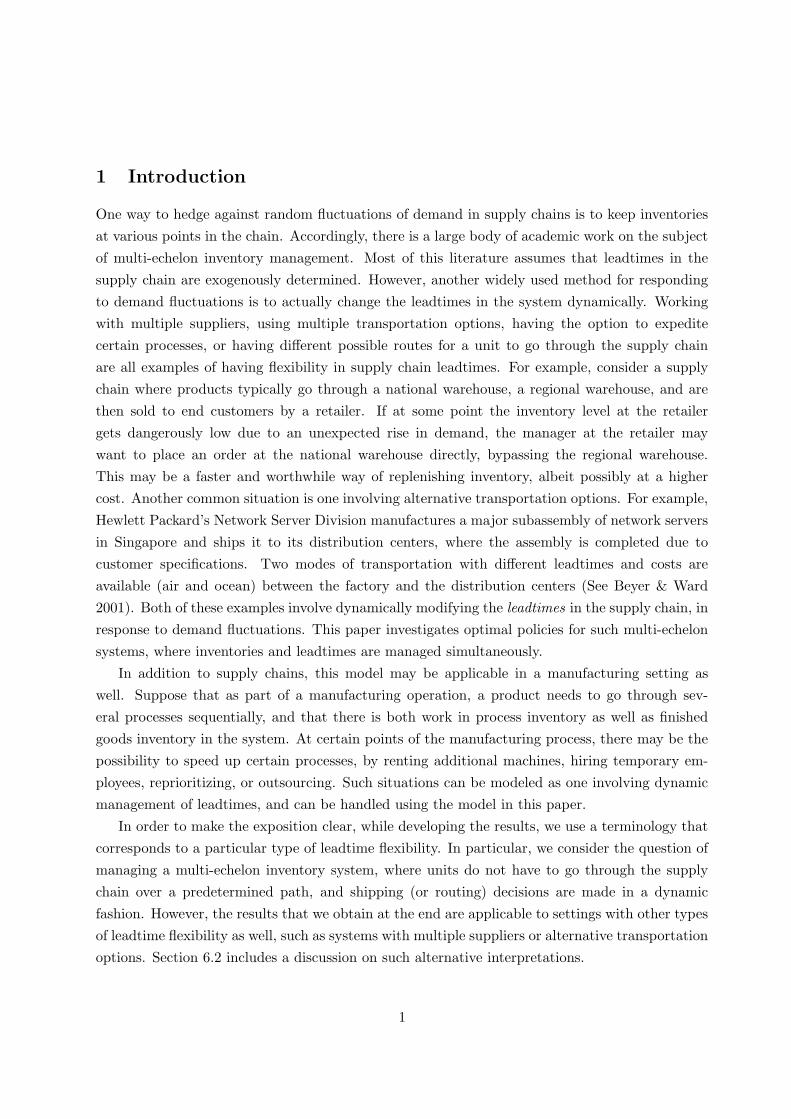
Figure 3: The figure shows the structure of the optimal policy for the single unit subproblem.Consider a certain stage z. The customer position axis is segmented into several intervals for thisstage, where the end points of the intervals are the extended echelon base stock levels. For a unitat stage z, the decision of whether and where to ship the unit depends on in which interval theposition of the corresponding customer falls. This figure depicts a situation, where the unit is atstage z = 4, the position y of the corresponding customer is 4, and S4,1

t = 0, S4,2t = 2, S4,3

t = 4.Since S4,2

t < y ≤ S4,3t , the unit is shipped to stage 3.

these extended echelon base stock levels as forming a measuring stick. When the echelon inventory

positions at stages 5 and 4 are compared against this measuring stick, the shipment decisions are

easily determined. Two cases are depicted on the top half of Figure 4. The case depicted on the

top left part of the figure corresponds to a situation where the echelon inventory position at stage

5 (I5) is 24 and the echelon inventory position at stage 4 (I4) is 5. This means that there are 19

units at stage 5. The policy dictates that out of these 19 units, 4 units will be kept at stage 5, 8

units will be shipped to stage 4, 3 units will be shipped to stage 3, and 4 units will be shipped to

stage 2. The picture on the top right corresponds to another case where I5 = 17 and I4 = −2.

We next give a formal definition of extended echelon base stock policies.

Definition 4.6. We say that a policy is of extended echelon base stock type if for every t and for

all pairs of stages (z, w), with z > w ≥ 1, there exist threshold values1 Sz,wt , which satisfy the

monotonicity properties in Lemma 4.3, so that the quantity to be shipped from stage z to stage

w at time t is2:(

(Izt ∧ Sz,w

t ) − (Iz−1t ∨ Sz,w−1

t ))+

.

The formula given in Definition 4.6 simply calculates the amount to be shipped from a stage

z to a stage w < z, given the echelon inventory positions at stages z and z − 1, according to the

procedure described in Figure 4. For example, let us consider the case shown on the top left part

of the figure, and let us calculate the amount to be shipped from stage 5 to stage 3. We have,

(

(I5 ∧ S5,3) − (I4 ∨ S5,2))+

= ((24 ∧ 12) − (5 ∨ 9))+ = 3.

1The threshold values are allowed to be an integer or −∞. Set Sz,0t = −∞ for all z and t.

2We define A ∨ B := max{A, B} and A ∧ B := min{A, B}

16

Figure 4: Illustration of Extended Echelon Base Stock Policies

17

For the amount shipped from stage 5 to stage 2, we have:

(

(I5 ∧ S5,2) − (I4 ∨ S5,1))+

= ((24 ∧ 9) − (5 ∨ 3))+ = 4.

Extended echelon base stock policies are very easy to implement. The informational require-

ments are minimal. Each stage z has a local manager responsible of shipments from stage z to

downstream stages, who is given a set of extended echelon base stock levels for her stage at the

beginning of the horizon. Then, as time progresses, the manager needs to monitor only the echelon

inventory position and the local inventory level at her stage z. The echelon inventory position at

stage z−1 is simply the difference between these two quantities. The amounts to be shipped from

z to downstream stages depend only on the extended echelon base stock levels for stage z and the

echelon inventory positions at stage z and z − 1, which the manager has information about.

Note that an echelon base stock policy is a special case of an extended echelon base stock

policy, with Sz,wt = −∞ for every w < z−1. In that case, the number of units shipped from stage

z to stages other than the next stage z − 1 are 0. The number of units shipped from stage z to

stage z − 1 are:(

(Izt ∧ Sz,z−1

t ) − Iz−1t

)+

which is exactly the number of units shipped from stage z to stage z − 1 under an echelon base

stock policy with base stock level Sz,z−1

t for stage z − 1. The bottom half of Figure 4 illustrates

how an echelon base stock policy is a special case of extended echelon base stock policies.

Theorem 4.1. The set of extended echelon base stock policies is optimal for finite horizon prob-

lems.

Proof. By an argument virtually identical to Lemma 2.1(3), choosing the decision according to

µt for every unit and every time step constitutes an optimal policy, for all initial states such that

the corresponding subproblem states are not of prohibited type.3 The resulting overall policy is

an extended echelon base stock policy.

5 Infinite Horizon Analysis

In the infinite horizon setting, we focus on stationary policies. A stationary policy is one of the

form (µ, µ, . . .), where the decision at each time is a function of the current state but not of the

current time.

Similarly, for the subproblems, we refer to a stationary policy of the form (µ, µ, . . .) as policy

µ. Given a fixed discount factor α ∈ [0, 1], let J µ∞(z, y) and J∗

∞(z, y) be the infinite horizon

3The difference here arises because Lemma 2.1(3) applies when µ is defined at all states, whereas we defined µ

at all states except for a set of states that are impossible to reach under any optimal policy.

18

expected total discounted cost of policy µ, and the corresponding optimal cost, respectively. Let

J µT (z, y) be the expected total discounted cost of using the stationary policy µ in a subproblem

over a finite horizon of length T , given that the initial state of the subproblem is (z, y).

The next lemma from Muharremoglu & Tsitsiklis (2001) relates the finite and infinite horizon

versions of the subproblem.

Lemma 5.1. For any fixed α ∈ [0, 1], and any z, y, we have

limT→∞

J∗T (z, y) = J∗

∞(z, y).

Furthermore, if u ∈ U∗t (z, y) for infinitely many choices of t, then u ∈ U∗

∞(z, y).

In Section 4.2, we showed that for finite horizon problems with horizon length T , an optimal

subproblem policy with a particular structure can be chosen, by constructing a table Mk(z, y) (like

the one in Figure 2) for each k ≤ T . We then showed that this subproblem policy, when applied

to all unit-customer pairs independently, results in an extended echelon base stock policy that

is optimal. In particular, the Mk(z, y) tables were constructed in a way such that a particular

control u was chosen from within the U∗k (z, y) sets for each z and y ≤ Ymax and remaining

time k ≤ T , such that the resulting committed and decoupled policy for the overall system is an

extended echelon base stock policy. The extended echelon base stock levels Sz,xt to be used at time

t = T − k only depend on the remaining time k, by construction. (Hence note that Sz,xT−k = Sz,x

T ′−k

for all T ′ ≥ T > k).

Proposition 5.1. There exists a k, such that the stationary policy µ that chooses its actions

according to µ(z, y) = Mk(z, y) for all (z, y), is optimal for the infinite horizon subproblem.

Proof. Consider the Mk(z, y) tables for different values of k. First note that the table entries

are values between 1 and Ymax. Since there is a fixed number of entries, there is a finite number

of possible tables, which means that at least one table is repeated for infinitely many choices of

k. Let k be such that Mk(z, y) = Mk(z, y) for all (z, y), and for infinitely many choices of k.

This means that, Mk(z, y) ∈ U∗k (z, y) for all (z, y) and for infinitely many k. By Lemma 5.1,

Mk(z, y) ∈ U∗∞(z, y) for all (z, y). Hence, µ is optimal for the infinite horizon subproblem.

Proposition 5.2. Let µ∗ be the stationary, decoupled, and committed policy for the overall prob-

lem that uses the optimal subproblem policy µ of Prop. 5.1 for each unit-customer pair. Then, µ∗

is a stationary extended echelon base stock policy.

Proof. Note that µ is constructed so that the prescribed actions are equivalent to the actions of

a finite horizon policy, when k periods are left. In particular, the policy is to ship units according

to extended echelon base stock levels Sz,x∞ = Sz,x

T−k, for some finite horizon problem with horizon

length T > k. The same levels are used in every period, so the policy is stationary.

19

We have so far constructed a stationary extended echelon base stock policy µ∗. This policy is

constructed as a limit of optimal policies for the corresponding finite horizon problems. It should

then be no surprise that µ∗ is optimal for the infinite horizon problem. Some careful limiting

arguments are needed to make this rigorous. However, these arguments are virtually identical to

the corresponding ones in Muharremoglu & Tsitsiklis (2001) and for this reason, the proof of the

following result is omitted.

Theorem 5.1. The set of extended echelon base stock policies is optimal for both the discounted

cost and the average cost criteria.

6 Discussion

We start this section by discussing some extensions to the model. Afterwards, we provide some

alternative interpretations of the results, corresponding to systems with different types of flexible

leadtimes. Finally, we investigate the special case where the shipping costs are additive, as in

Lawson & Porteus (2000). The assumption of additive costs simplifies the problem, and results in

simpler policies. In particular, we show that our decomposition approach leads to results similar

to the ones in Lawson & Porteus (2000).

6.1 Extensions

In this subsection, we discuss some possible extensions to our model. In particular, we focus on

the leadtime and demand models.

In our model, the leadtimes for shipping from one stage to any other stage were assumed

to be equal to one period. However, in many real world systems, longer leadtimes may be

required. Such systems can be modeled within our framework, by converting them to equivalent

unit leadtime systems. (This is done by introducing artificial locations between stages, and by

setting appropriate shipping and holding costs to capture the dynamics of the system correctly.)

However, our approach and results will only apply if the resulting shipping cost structures are

supermodular. For instance, if we have two stages z and z − 1 with a multi period leadtime

between them, any model with a finite cost and faster shipping option (where the difference is

more than one period) from a stage w ≥ z to a stage v ≤ z − 1 would result in a structure that is

not supermodular and cannot be handled by our model. In this case, it may be optimal for units

to overtake each other and optimal policies may potentially be more complicated than simple

threshold policies. The only way to avoid this would be to allow convertible leadtimes, where

a unit that is already in transit between z and z − 1 via the slow transportation mode can be

converted to the expedited mode while still in transit.

So, our analysis does not apply to situations that correspond to systems with shipping costs

that are not supermodular. This raises the question whether another approach can yield the same

20

result for such systems in general. The answer is no, since in such a case, optimal policies may be

potentially much more complicated and dependent on the state of outstanding orders. This fact

is illustrated in the next subsection, where systems with dual suppliers are considered using our

model.

Another possible extension is to allow for stochastic leadtimes. Our method can handle

stochastic leadtimes of the type used in Muharremoglu & Tsitsiklis (2001). However, again,

we need to make sure that in any such model, the supermodularity assumption is satisfied.

We can also handle the more general case of Markov-modulated demand, as in Muharremoglu

& Tsitsiklis (2001). In this case, the extended echelon base stock levels will of course depend on

the state of the modulating Markov chain.

Finally, note that we have not given an explicit algorithm that determines the extended echelon

base stock levels. However, since we have shown that the problem can be decomposed into single-

unit subproblems, the extended base stock levels can easily be determined by solving a single

unit subproblem. Such a problem is quite simple to solve using dynamic programming. Once the

subproblem is solved and the optimal action sets U are determined, the extended echelon base

stock levels are readily available.

6.2 Alternative Interpretations

While developing the results in previous sections, we used a terminology that corresponds to

making shipping (or routing) decisions in a multi-echelon inventory systems. However, the system

that we analyzed can also be used to model settings where different types of leadtime flexibility

are present. In this subsection, we describe one such interpretation, that corresponds to using

multiple suppliers in a single stage system with different leadtimes and costs.

Consider the manager of a single retail store that buys a durable product from suppliers and

sells it to customers. In order to manage the uncertainty in customer demand, the manager keeps

inventories of the product in the store. The store has a relationship with two different suppliers

that provide the same product. One supplier is located closer to the store and can respond faster

to orders. The other supplier is located further away and takes longer to fulfill orders; however, it

charges a lower per unit price for the product. The manager can choose to place orders at either

one of the suppliers at any time. The goal is to use inventories and the multiple suppliers to

respond to fluctuations in customer demand, by managing the leadtime-cost tradeoff in the best

way possible.

This problem is an example for a single stage inventory problem with dual supply options,

which has been analyzed in numerous papers, some of which were listed in the introduction. The

only available optimality results for this problem with simple policies correspond to cases where

the suppliers’ leadtimes differ by only one period. If the leadtime from the slow supplier and the

fast supplier differ by more than one period, optimal policies are more complicated (than extended

21

echelon base stock policies), as shown by Whittemore & Saunders (1977). This is illustrated in

Figure 5, where two cases of a dual supplier problem are depicted. In case 1, the slow and fast

suppliers have leadtimes of k and k + 1, respectively, whereas in case 2, the leadtimes are k − 1

and k + 1. Let cF be the cost that the fast supplier charges, and cS the cost that the slow

supplier charges, for a single unit of the product. To model these two situations as special cases

of our formulation, we first visualize the two suppliers as a single aggregated supplier and insert

k − 1 artificial locations between the aggregated supplier and the retailer. We model the choice

of different suppliers as using different paths while shipping units from the aggregate supplier to

the retailer. Consider case 1. Units that are ordered from the slow supplier go through locations

k+2, k+1, k, k−1, . . . , 1, which takes k+1 periods, and incur a cost of cS . Units that are ordered

from the fast supplier skip location k +1, so that they are delivered in k periods, and incur a cost

of cF . To model the fact that a leadtime of less than k is impossible, we set some shipping costs

equal to infinity, such as ck+2,k−1, ck+2,k−2, or c3,1, etc. Also, we need to set the holding costs at

the artificial stages to a large enough value to ensure that units are not delayed while in transit.

With this formulation, the dual supplier problem is a special case of our formulation.

First, notice that supermodularity is satisfied in case 1. This means that our analysis is

applicable, and extended echelon base stock policies are optimal. The interpretation of extended

echelon base stock policies in this setting is as follows: There are two different reorder levels

corresponding to the two suppliers, say RF for the fast supplier and RS for the slow supplier,

where RS > RF . The optimal policy compares the inventory position I of the retailer (on hand

inventory + outstanding orders - backlog) to these levels when making ordering decisions. In

particular, the optimal ordering policy is:

If I ≥ RS , order nothing.

If RF ≥ I > RS , order I − RS units from the slow supplier.

If I > RF , order RF − RS units from the slow and I − RF units from the fast supplier.Now, notice that while supermodularity is satisfied in case 1, it is not satisfied in case 2,

because we have:

ck+2,k−1 + ck,k = cF + 0 < ck+2,k + ck,k−1 = ∞ + 0

This implies that monotonic policies are not necessarily optimal for case 2, and the problem

cannot be decomposed into single unit subproblems. Consequently, optimal policies are not

guaranteed to be simple threshold type policies that depend only on the inventory position of the

store. This is consistent with the existing results in the literature.

6.3 The Case of Additive Costs

The paper by Lawson & Porteus (2000) deals with a problem that is very similar to ours, i.e., a

serial system with leadtime flexibility. They present their model a little differently, though. In

22

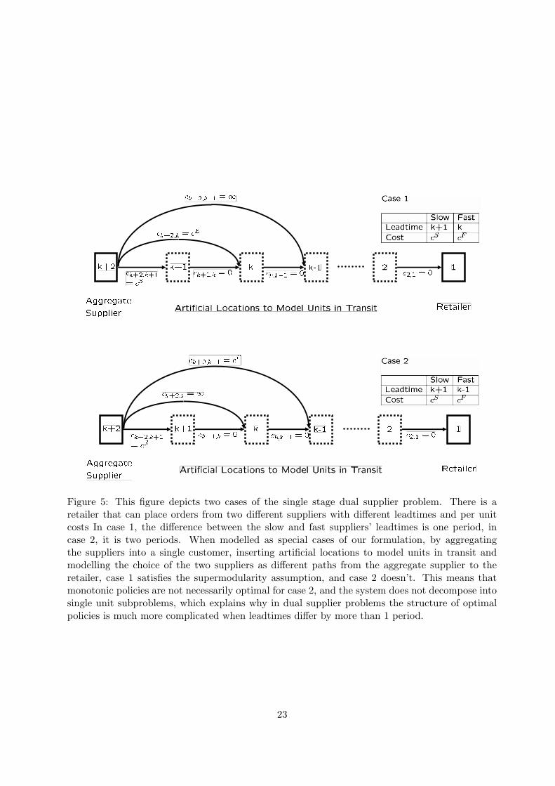
Figure 5: This figure depicts two cases of the single stage dual supplier problem. There is aretailer that can place orders from two different suppliers with different leadtimes and per unitcosts In case 1, the difference between the slow and fast suppliers’ leadtimes is one period, incase 2, it is two periods. When modelled as special cases of our formulation, by aggregatingthe suppliers into a single customer, inserting artificial locations to model units in transit andmodelling the choice of the two suppliers as different paths from the aggregate supplier to theretailer, case 1 satisfies the supermodularity assumption, and case 2 doesn’t. This means thatmonotonic policies are not necessarily optimal for case 2, and the system does not decompose intosingle unit subproblems, which explains why in dual supplier problems the structure of optimalpolicies is much more complicated when leadtimes differ by more than 1 period.

23

particular, they have a system where the units have to go through all the stages in this serial

system. The transition from one stage to the next can take one period (via the regular shipment

method) or can be instantaneous, which is called expedited delivery. The expedited delivery and

the regular shipment from a stage to the next each have a particular cost associated with them.

In addition, a unit can be expedited through several stages in the system within the same period.

Such a transition can also be viewed as transferring the unit from a stage to another by skipping

others in between, just like in our model. The main difference is that Lawson & Porteus (2000)

use an additive cost structure, meaning that the cost of expediting through several stages is equal

to the sum of the one step expediting costs. Our model assumes a more general cost structure,

namely supermodularity, which includes additive costs as a special case.

Still, the policies reported in Lawson & Porteus (2000) are slightly different than our extended

echelon base stock policies. The reason is one more difference between the two papers about the

sequence of events within a period. In particular, in Lawson & Porteus (2000), in every period

two sets of decisions are made. (See Figure 6). First, expediting decisions are made, which take

place instantaneously. Here, any unit can be transferred from any stage to any downstream stage

through a series of one stage expediting decisions, which is just like our expediting model. Then,

regular order decisions are made, and these orders are not delivered until the beginning of the

next period. Such a setting can easily be analyzed by our approach as well. We didn’t use this

setting in the previous sections just to simplify the exposition. We could model such a two step

decision process by having alternating “expediting periods” and“regular order periods”, where

an actual period corresponds to one expediting and one regular order period in the model. In

expediting periods, we would be able to send units from any stage to any downstream stage.

There would be no customer arrivals and no holding or backorder costs in expediting periods, just

origin-destination dependent shipment costs. Then, in regular order periods, we could only ship

units to the next stage. The customer arrivals and the charging of holding and backorder costs

would occur in regular order periods. The single unit analysis can easily be applied to this setting

as well. The optimal policy in this case is to use extended echelon base stock policies in expediting

periods and echelon base stock policies in regular order periods. In addition, the extended echelon

base stock levels in this case have a very special structure due to the additivity of the expediting

costs, as shown by the following proposition. Let Sz,wt be the extended echelon base stock levels

for shipments originating at stage z destined to stage w at time t. (For z > w ≥ 1).

Proposition 6.1. Sz,wt = Sz−1,w

t for all z, w ≤ z − 2, and all t.

Proof. Suppose that the proposition is not true. There are two cases: (In the rest of the proof,

we suppress the dependency on t to simplify the expressions).

(a) Suppose that Sz,w < Sz−1,w for some z and w ≤ z − 2. By the definition of the extended

echelon base stock levels, we know that M(z, Sz,w+1) = v for some v > w. By the definition

24

Figure 6: The sequence of events assumed by Lawson & Porteus.

of M(·), this means that v ∈ U∗(z, Sz,w + 1), i.e., if the subproblem state is (z, Sz,w + 1),

then it is optimal to ship the unit from z to v. This implies that

cz,v + J(v, Sz,w + 1) ≤ cz,r + J(r, Sz,w + 1),

for any r. (Here, J(·, ·) is the optimal cost-to-go function for the subproblem at the end of

the expediting period.) The expediting costs are additive, meaning that cz,r = cz,v + cv,r.

Thus,

J(v, Sz,w + 1) ≤ cv,r + J(r, Sz,w + 1), (2)

for any r.

By the definition of the extended echelon base stock levels and by the assumption that

Sz,w < Sz−1,w, we have M(z− 1, Sz,w +1) = r for some r ≤ w. This, together with the fact

that M(z, Sz,w + 1) = v implies that v /∈ U∗(z − 1, Sz,w + 1). Hence,

cz−1,v + J(v, Sz,w + 1) > cz−1,r + J(r, Sz,w + 1).

Since cz−1,r = cz−1,v + cv,r, we obtain

J(v, Sz,w + 1) > cv,r + J(r, Sz,w + 1). (3)

Inequalities (2) and (3) are contradictory.

(b) Suppose that Sz,w > Sz−1,w for some z and w ≤ z − 2. By the definition of the extended

echelon base stock levels, we know that M(z−1, Sz,w) = v for some v > w. By the definition

of M(·), this means that v ∈ U∗(z − 1, Sz,w), i.e., if the subproblem state is (z − 1, Sz,w),

then the decision to ship the unit from z − 1 to v is an optimal one. This implies that

cz−1,v + J(v, Sz,w) ≤ cz−1,r + J(r, Sz,w),

25

for any r. The expediting costs are additive, meaning that cz−1,r = cz−1,v + cv,r. Thus,

J(v, Sz,w) ≤ cv,r + J(r, Sz,w), (4)

for any r.

By the definition of the extended echelon base stock levels and by the assumption that

Sz,w > Sz−1,w, we have M(z, Sz,w) = r for some r ≤ w. This, together with the fact that

M(z − 1, Sz,w) = v implies that v /∈ U∗(z, Sz,w). Hence,

cz,v + J(v, Sz,w) > cz,r + J(r, Sz,w).

Since cz,r = cz,v + cv,r,

J(v, Sz,w) > cv,r + J(r, Sz,w). (5)

Inequalities (4) and (5) are contradictory.

Hence, we have shown that in the model where expediting costs are additive and expediting

takes place instantaneously, we only need M threshold values for expediting decisions, instead of

M(M + 1)/2. In particular, we have values Sw such that SM+1,w = SM,w = · · · = Sw+1,w = Sw,

for all w. These values are exactly the expediting base stock levels in Lawson & Porteus (2000).

In addition, we have regular base stock levels for the regular order periods. These are the regular

order base stock levels in Lawson & Porteus (2000). The policy of making expediting decisions

according to the expediting base stock levels and then regular order decisions according to the

regular order base stock levels is exactly what was coined as “top-down echelon base stock policies”

in Lawson & Porteus (2000).

7 Conclusions

Having some sort of flexibility in leadtimes is a very commonly utilized method of managing

uncertainty in supply chains. Working with multiple suppliers, using multiple transportation

options, having the option to expedite certain processes, or having different possible routes for

a unit to go through the supply chain are all examples of having flexibility in the supply chain

leadtimes. In this paper, we introduced a formulation that can be used to model such problems

where the objective is to control inventories and leadtimes simultaneously in order to minimize

costs in the supply chain. Under a certain supermodularity assumption on the costs, we charac-

terized the structure of optimal policies as extended echelon base stock policies, which is a natural

generalization of the well known echelon base stock policies. Extended echelon base stock policies

26

are quite intuitive and require minimal information sharing among different stages of the supply

chain for implementation.

Our main analysis technique was to decompose the problem into a series of single-unit single-

customer problems, and then to analyze the structure of the subproblems. This approach, besides

being a proof technique, also gives rise to efficient algorithms for calculating the extended ech-

elon base stock levels. In particular, to determine these threshold values, we only need to solve

one subproblem with a single unit and a single customer, which can be achieved by solving a

straightforward and simple dynamic programming problem.

While the set of supermodular costs is quite a large set, one can certainly think of many real

world systems where this assumption would not be a reasonable one. We know that a complete

relaxation of this assumption may lead to complicated policies that depend on the state of the

outstanding orders. However, one interesting research question is whether there are other cost

structures that still result in simple policies. Another equally intriguing question is, how do

extended echelon base stock policies perform for systems where the supermodularity assumption

is not satisfied? Finally, designing a system with leadtime flexibility may in itself involve a cost.

What is the best way to manage the tradeoff between this cost and the benefits of having the

flexibility?

Acknowledgement

This research was partially supported by the National Science Foundation under grant ACI-

9873339.

References

Anupindi, R. & Akella, R. (1993), ‘Diversification under supply uncertainty’, Management Science

39, 944–963.

Barankin, E. (1961), ‘A delivery-lag inventory model with an emergency provision’, Naval Re-

search Logistics Quarterly 8, 285–311.

Beyer, D. & Ward, J. (2001), Network server supply chain at HP: A case study, in J. S. Song

& D. Yao, eds, ‘Supply Chain Structures: Coordination, Information and Optimization’,

Kluwer Academic Publishers, Boston, MA, chapter 8.

Chen, F. & Zheng, Y. (1994), ‘Lower bounds for multi-echelon stochastic inventory systems’,

Management Science 40, 1426–1443.

27

Chiang, C. & Gutierrez, G. (1998), ‘Optimal control policies for a periodic review inventory

system with emergency orders’, Naval Research Logistics 45, 187–204.

Clark, A. & Scarf, S. (1960), ‘Optimal policies for a multi-echelon inventory problem’, Management

Science 6, 475–490.

Daniel, K. (1963), A delivery-lag inventory model with emergency, in H. Scarf, G. D & S. M, eds,

‘Multistage Inventory Models and Techniques’, Stanford University Press, Stanford, CA.

Federgruen, A. & Zipkin, P. (1984), ‘Computational issues in an infinite horizon, multi-echelon

inventory model’, Operations Research 32, 818–836.

Fukuda, Y. (1964), ‘Optimal policies for the inventory problem with negotiable leadtime’, Man-

agement Science 10, 690–708.

Gallego, G., Sethi, S., Yan, H., Zhang, H. & Huang, Y. (2002), A periodic review inventory model

with three delivery modes and forecast updates. Working Paper, School of Management, the

University of Texas at Dallas.

Huggins, E. & Olsen, T. (2002), Supply chain management with overtime and premium freight.

Working Paper, Olin School of Business, Washington University in St. Louis.

Lawson, D. & Porteus, E. (2000), ‘Multi-stage inventory management with expediting’, Operations

Research 48, 878–893.

Moinzadeh, K. & Nahmias, S. (1988), ‘A continuous review model for an inventory system with

two supply modes’, Management Science 34, 761–773.

Moinzadeh, K. & Schmidt, C. (1991), ‘An (s-1,s) inventory system with emergency orders’, Op-

erations Research 39, 308–321.

Muharremoglu, A. & Tsitsiklis, J. (2001), Echelon base stock policies in uncapacitated serial

inventory systems. Working Paper, Submitted, Massachusetts Institute of Technology, Cam-

bridge, MA.

Swaminathan, J. & Shanthikumar, G. (1999), ‘Supplier diversification: Effect of discrete demand’,

Operations Research Letter 24, 213–221.

Whittemore, A. & Saunders, S. (1977), ‘Optimal inventory under stochastic demand with two

supply options’, SIAM Journal of Applied Mathematics 32, 293–305.

Zhang, V. (1996), ‘Ordering policies for an inventory system with three supply modes’, Naval

Research Logistics 43, 691–708.

28