1

Dynamic Female Labor Supply

Zvi Eckstein and Osnat Lifshitz

December 27, 2010Based on the Walras-Bowley Lecture to the American Econometric Society

Summer meeting, June 2008

Why Do We Study Female

Employment (FE)?

3

Because they contribute a lot to US Per Capita GDP…

Actual

Labor Input Fixed at 1964

15000

20000

25000

30000

35000

40000

45000

1964 1968 1972 1976 1980 1984 1988 1992 1996 2000 2004

year2006 prices.

43797 (244%)

40%Actual

Labor Input Fixed at 1964Labor Quality Input

Fixed at 1964

15000

20000

25000

30000

35000

40000

45000

1964 1968 1972 1976 1980 1984 1988 1992 1996 2000 2004

year2006 prices.

43797 (244%)

40%

Central Question

Why Did Female Employment (FE)

Rise Dramatically?

5

Because Married FE Rose…..!Employment Rates by Marital Status - Women

Married

Single

0%

10%

20%

30%

40%

50%

60%

70%

80%

90%

100%

1962 1966 1970 1974 1978 1982 1986 1990 1994 1998 2002 2006

yearAges 22-65. Proportion of women working 10+ weekly hours.

Employment Rates by Marital Status - Women

Married

Single

Divorced

0%

10%

20%

30%

40%

50%

60%

70%

80%

90%

100%

1962 1966 1970 1974 1978 1982 1986 1990 1994 1998 2002 2006

yearAges 22-65. Proportion of women working 10+ weekly hours.

7

Why did Married Female Employment (FE)

Rise Dramatically?

Main Empirical Hypotheses Schooling Level increase (Becker)

Wage increase/Gender Gap decline Heckman and McCurdy(1980), Goldin(1990), Galor and Weil(1996), Blau and Kahn(2000), Jones, Manuelli and McGrattan(2003), Gayle and Golan(2007)

Fertility decline Gronau(1973), Heckman(1974), Rosensweig and Wolpin(1980), Heckman and Willis(1977), Albanesi and Olivetti(2007) Attanasio at.al.(2008)

Marriage decline/Divorce increase Weiss and Willis(1985,1997), Weiss and Chiappori(2006)

Other – (unexplained)

Schooling Level IncreaseBreakdown of Married Women by Level of Education

High School Dropouts

High School Graduates

Some College

College Graduates

Post College

0%

5%

10%

15%

20%

25%

30%

35%

40%

45%

50%

1964 1968 1972 1976 1980 1984 1988 1992 1996 2000 2004

yearAges 22-65.

10

Wage increase – Gender Gap declineAnnual Wages of Full-Time Workers

Men

Women

Women to Men Wage Ratio (right axis)

0

10000

20000

30000

40000

50000

60000

70000

1962 1966 1970 1974 1978 1982 1986 1990 1994 1998 2002 2006

year

45%

50%

55%

60%

65%

70%

75%

80%

Ages 22-65. Full-time full-year workers with non-zero wages. 2006 Prices.

Annual Wages of Full-Time Workers

Men

Women

Women to Men Wage Ratio (right axis)

0

10000

20000

30000

40000

50000

60000

70000

1962 1966 1970 1974 1978 1982 1986 1990 1994 1998 2002 2006

year

45%

50%

55%

60%

65%

70%

75%

80%

Ages 22-65. Full-time full-year workers with non-zero wages. 2006 Prices.

11

Fertility Decline

Ref.

by cohort

Number of Children per Married Women

Children under 6

Children under 18

0.0

0.2

0.4

0.6

0.8

1.0

1.2

1.4

1.6

1.8

1963 1967 1971 1975 1979 1983 1987 1991 1995 1999 2003 2007

yearAges 22-65. Extrapolated data for number of young children during 1968-1975.

13

Marriage Declines – Divorce Increases Breakdown of Women by Marital Status

Married

Single (Never Married)

Divorced

0%

10%

20%

30%

40%

50%

60%

70%

80%

90%

100%

1962 1966 1970 1974 1978 1982 1986 1990 1994 1998 2002 2006

yearAges 22-65.

What are the Other Empirical Hypotheses?

Social Norms Fernandez, Fogli and Olivetti(2004), Mulligan and Rubinstein(2004), Fernandez (2007)

Cost of Children Attanasio, Low and Sanchez-Marcos(2008) Albanesi and Olivetti(2007)

Technical Progress Goldin(1991), Greenwood et. al.(2002),

Will show up as a cohort effects..

15

Post baby-boomers Cohort’s FE stabilizedEmployment rates by Age

Married Female Employment Rates by Cohort

Born 1925

Born 1935

Born 1945

Born 1955

Born 1965Born 1975

0%

20%

40%

60%

80%

22 26 30 34 38 42 46 50 54 58 62

ageYears 1962-2007. Proportion of women working 10+ weekly hours.

An Accounting Exercise Measure female’s employment due to:

Schooling Level increase

Wage increase/Gender Gap decrease

Fertility decline

Marriage decline/Divorce growth

The “unexplained” is Others

Lee and Wolpin, 2008

An Accounting Exercise

Need an empirical model Use Standard Dynamic Female Labor Supply Model

– Eckstein and Wolpin 1989 (EW): “old” model

Later extensions (among others..): van der Klauw, 1996, Altug

and Miller, 1998, Keane and Wolpin, 2006 and Ge, 2007.

Sketch of the Model Extension of Heckman (1974) Female maximizes PV utility

Chooses employment (pt = 1 or 0)

Takes as given:

Education at age 22

Husband characteristics

Processes for wages, fertility, marital status

Estimation using SMM and 1955 cohorts from CPS

Model

Estimation Fit – 1955 cohort FE

24

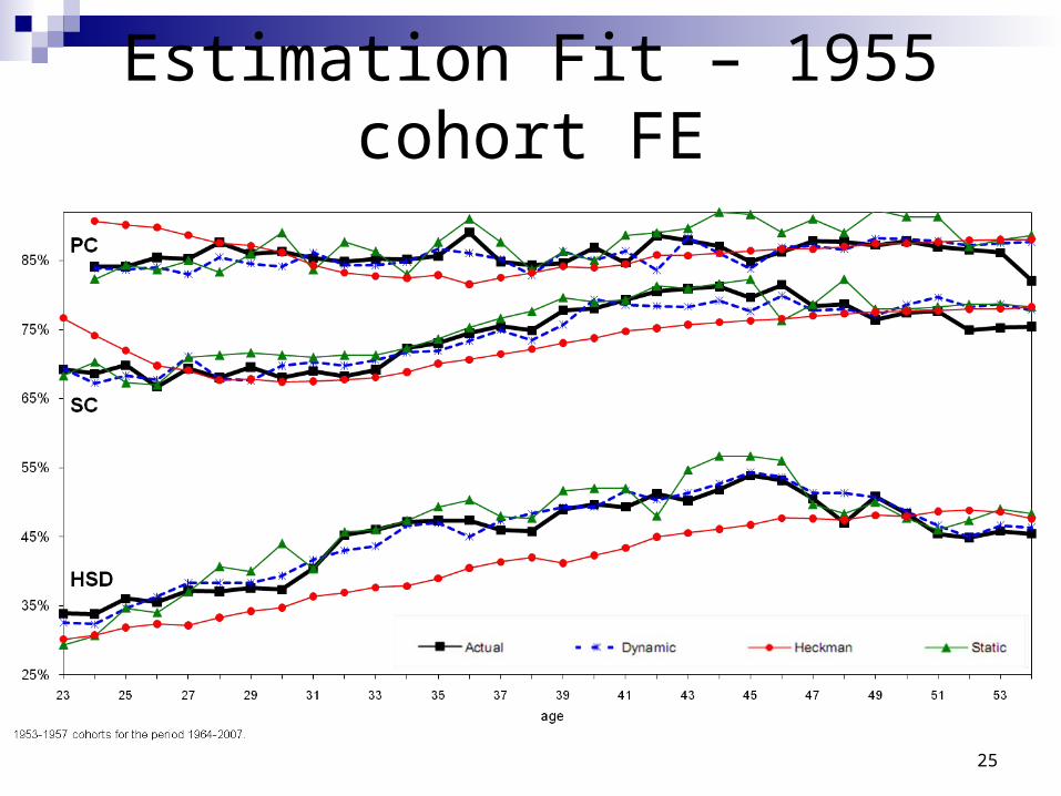
Estimation Fit – 1955 cohort FE

25

Estimation Fit – 1955 cohort FE

26

Back to Accounting Exercise For the 1955 cohort we estimated:

p55= P55(S, yw, yh, N, M) for each age

Contribution of Schooling of 1945 cohort (S45) for predicted FE of 1945 cohort is:

predicted p45= P55(S45, yw55, yh55, N55, M55)

….Schooling and Wagepredicted p45= P55(S45, yw45, yh45, N55, M55)

….Etc

FE by Age per Cohort

Actual 1925

Actual 1935

Actual 1945Actual 1955

Actual 1965

Actual 1975Predicted 1955

30%

40%

50%

60%

70%

80%

23 25 27 29 31 33 35 37 39 41 43 45 47 49 51 53

ageYears 1964-2007.

1%Other

69%+ 4 Marital Status

69%+ 3 Children

69%1+ 2 Wage

71%1 - Schooling

68%Actual 1945

Age Group: 38-42 1955:Actual: 74% Fitted: 74% 

12%Other

61%+ 4 Marital Status

+ 3 Children

63%1+ 2 Wage

63%1 - Schooling

49%Actual 1945

Age Group: 28-32 1955: Actual: 65% Fitted: 65%

Accounting for changes in FE: 1945 cohortDynamic Model

Early age total difference 12% is Other

61%

Goodness of Fit Tests for the Three Models

34

Pearson* SSD** Pearson* SSD** Pearson* SSD**

HSD 7.96 71.93 26.65 238.42 112.53 897.94

HSG 6.24 83.44 12.58 167.33 29.60 394.77

SC 5.95 90.04 10.46 157.99 25.32 376.86

CG 4.69 75.73 10.89 175.86 11.49 180.97

PC 6.23 106.56 16.06 286.98 15.50 268.18

ALL 31.06 427.71 76.64 1026.59 194.43 2118.71

Dynamic Static Heckman

35

Accounting for the change in FE:Cohorts of 1925, 30, 35 based on 1955

Dynamic Static Heckman

Schooling +initial 36% 33% 42%

Wage 23% 10% 0%

Children 4% 5% 14%

Martial Status 0% 1% 0%

Other 37% 51% 43%

Other - less than 38

Other - over 38 34% 48% 45%

1925-1935

no data

36

Accounting for the change in FE:Cohorts of 1940, 45, 50: based on 1955

Dynamic Static Heckman

Schooling +initial 33% 32% 39%

Wage 22% 9% 1%

Children 8% 7% 5%

Martial Status 1% 0% 0%

Other 36% 51% 55%

Other - less than 38 55% 63% 55%

Other - over 38 18% 40% 55%

1940-1950

37

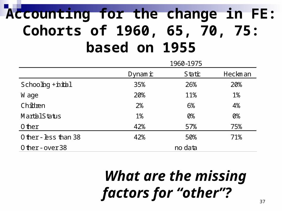
Accounting for the change in FE:Cohorts of 1960, 65, 70, 75: based on 1955

What are the missing factors for “other”?

Dynamic Static Heckman

Schooling +initial 35% 26% 20%

Wage 20% 11% 1%

Children 2% 6% 4%

Martial Status 1% 0% 0%

Other 42% 57% 75%

Other - less than 38 42% 50% 71%

Other - over 38

1960-1975

no data

What is missing factor for early ages?

Childcare cost if working

Change 1 parameter (– get perfect fit

1945 cohort childcare cost: $3/hour higher 1965 cohort childcare cost: $1.1/hour lower1975 cohort childcare cost: $1.1/hour lower

What is missing factor for all ages?

Childcare cost if working Value of staying at home Change 2 parameters (– get perfect fit

1935,1925 cohorts childcare cost: $3.2/hour higher 1935 cohort leisure value: $4.5/hour higher1925 cohort leisure value: $5/hour higher

How can we explain results?

Actual and Predicted Employment Rates 1940 Cohort

40

Actual and Predicted Employment Rates 1930 Cohort

41

42

How can we explain results?

Change in cost/utility interpreted as:

Technical progress in home productionChange in preferences or social norms

How do we fit the aggregate employment/participation?

Aggregate fit Simulation

Simulate the Employment rate for all the cohorts: 1923-1978.

Calculate the aggregate Employment for each cohort at each year by the weight of the cohort in the population.

Compare actual to simulated Employment 1980-2007.

Predicted Aggregate Female Employment RatesDynamic Model

Actual - Married

Actual - Unmarried

Predicted - Married

Predicted - Unmarried

50%

60%

70%

80%

1980 1982 1984 1986 1988 1990 1992 1994 1996 1998 2000 2002 2004 2006

yearAges 23-54.

Predicted Aggregate Female Employment Ratesby Cohort and Age - Dynamic Model

Age Group: 23-27 Actual Fitted Actual Fitted Actual Fitted Actual Fitted Actual Fitted Actual Fitted Actual Fitted Actual Fitted Actual Fitted ActualFitted

married 0.32 0.30 0.39 0.39 0.48 0.48 0.60 0.61 0.64 0.63 0.66 0.64 0.65 0.65

unmarried 0.74 0.70 0.73 0.72 0.71 0.69 0.71 0.69 0.72 0.72 0.72 0.72 0.76 0.74

Age Group: 28-32

married 0.30 0.31 0.36 0.40 0.43 0.45 0.55 0.57 0.65 0.68 0.68 0.69 0.69 0.68 0.66 0.67

unmarried 0.71 0.70 0.69 0.71 0.70 0.69 0.73 0.71 0.72 0.71 0.73 0.73 0.79 0.75 0.76 0.75

Age Group: 33-37

married 0.36 0.38 0.41 0.41 0.47 0.49 0.56 0.59 0.63 0.64 0.70 0.71 0.70 0.71 0.68 0.71

unmarried 0.68 0.67 0.67 0.66 0.67 0.67 0.72 0.71 0.75 0.73 0.74 0.71 0.77 0.75 0.76 0.74

Age Group: 38-42

married 0.40 0.42 0.45 0.47 0.51 0.50 0.59 0.59 0.66 0.65 0.71 0.70 0.73 0.74 0.72 0.73

unmarried 0.72 0.73 0.69 0.67 0.67 0.66 0.72 0.73 0.75 0.76 0.78 0.75 0.78 0.75 0.76 0.75

Age Group: 43-47

married 0.48 0.46 0.51 0.49 0.58 0.57 0.64 0.63 0.72 0.71 0.75 0.74 0.75 0.75

unmarried 0.70 0.71 0.68 0.69 0.71 0.71 0.73 0.75 0.77 0.76 0.78 0.76 0.76 0.75

Age Group: 48-52

married 0.48 0.49 0.53 0.53 0.59 0.58 0.65 0.65 0.71 0.71 0.74 0.74

unmarried 0.66 0.70 0.67 0.67 0.69 0.68 0.73 0.73 0.76 0.75 0.76 0.77

1960 1965 1970 1975

Cohort1925 1930 1935 1940 1945 1950

Alternative Modeling for Explaining “Other Gap”

Unobserved heterogeneity regarding leisure/cost of children

Bargaining power of women changes

Household game: a “new” empirical framework

46

47

Concluding remarks We demonstrate the gains from using Stochastic

Dynamic Discrete models: Dynamic selection method, rational expectations,

and cross-equations restrictions are imposed Accounting for alternative explanations for rise in

US Female EmploymentBetter fit than static models (new version)

Education – 35% of increase in Married FE Other – 25-45% of increase in Married FE Change in two parameters close the Other Gap

Thanks!!