DYNAMIC EVOLVEMENT ASSESSMENT AND …portal.dl.saga-u.ac.jp/bitstream/123456789/122399/1/quan_201406.pdf · technology of geographic information system ... Dynamic evolvement assessment

－ 36 －

LOWLAND TECHNOLOGY INTERNATIONAL Vol. 16, No.1, 36-44, June 2014 International Association of Lowland Technology (IALT), ISSN 1344-9656

DYNAMIC EVOLVEMENT ASSESSMENT AND FORECAST OF LAND USE BASED ON

GEOGRAPHIC INFORMATION SYSTEM

Dongjie Guan 1＊, Xiaosong Lin 2, Weijun Gao 3, Weici Su 4 and Kazunori Hokao 5

ABSTRACT: Based on the land use patterns in the years of 1990, 1995, 2000 and 2005 acquired with the spatial technology of geographic information system (GIS), this study takes Kitakyushu city in Japan as a case to analyze and forecast the dynamic change and transformation of various land use types. Firstly, we use the spatial distribution maps to describe the changes of area and spatial distribution of land use in the past 15 years, and then the dynamic change models are established to evaluate the changes of speed and intensity of land use. The results indicate that each land use type has changed remarkably as the urbanization, and that the land use intensity has been transferring from extensive type to intensive type. Finally, we develop a transfer matrix of Markov to track the mutual transformation processes among the land use types, and to forecast the change tendency of future land use. The forecasting results reveal that the urban land will keep increasing at a decelerated speed, and it will be a long process for land use intensity to reach to the urbanization level. Keywords: Land use, geographic information system, dynamic change model, Markov model

1* Hehai College, Chongqing Jiaotong University, Chongqing 400074, CHINA, [email protected]; [email protected]

2 Hehai College, Chongqing Jiaotong University, Chongqing 400074, CHINA 3 Faculty of Environmental Engineering, The University of Kitakyushu, 808-0135, Kitakyushu, JAPAN 4 Faculty of Geographic Science, Chongqing Normal University, Chongqing 400074, CHINA 5 Faculty of Science and Engineering, Saga University, 840-8502, Saga, JAPAN Note: Discussion on this paper is open until December 2014

INTRODUCTION

Land use change plays vital roles in regional, social and economic development, and global environmental changes (Turner et al. 1993). In 1995, International Geosphere-Biosphere Program (IGBP) and International Human Dimensions Program (IHDP) launched a plan of “Land Use/Cover Change (LUCC)” to investigate the huge land use changes caused by growing industrialization and urbanization (Meyer and Turner 1996; Geist and Lambin 2001; Susanna and Chen 2002; Erika et al. 2005). Since then LUCC has been an advanced subject in urban development and environment change. Various methodologies and algorithms have been applied to elucidate land use/cover change information from different remotely sensed data. In an international comprehensive view, studies on LUCC can be summarized as three core issues: dynamic analysis of process, driving forces, and evaluation models of LUCC ((Herold et al. 2002; Gautam et al., 2003; Patma et al. 2004; Quan et al. 2006; Luciana et al. 2007).

In recent years, LUCC community has produced a large set of operational models that can be used to predict or explore possible land use/cover change

trajectories (Verburg et al. 2006). Models can support the exploration of future land use/cover changes under different scenario conditions. Moreover, scenario analysis with land use/cover models can support land use/cover planning and policy. All these models are divided into three classes: empirical and statistical models, such as Markov chains and Regression model, etc.; dynamic models, such as Cellular automata(CA) model, Agent-based model and System dynamic model etc.; integrated model, such as CLUE (Conversion of Land Use and its Effects) model etc. Empirical and statistical models can complement dynamic simulation. Dynamic models are suited to predict future land use/cover changes superior to empirical and statistical models. An integrated model that combines multidiscipline and elements of different modeling techniques will probably improve the understanding of land use change processes. For example, Asif et al. (2005) addressed a multi-temporal analysis of land use change using Thematic Mapper (TM) data from 1986 to 2000 in Nagasaki City, Japan. Wu and Ci (2002) assessed the land use change in the Mu Us Sandy Land of northern China from the 1950s to the 1990s through analysis of satellite images, historical maps,

－ 37 －

Dynamic evolvement assessment and forecast of land use based on GIS

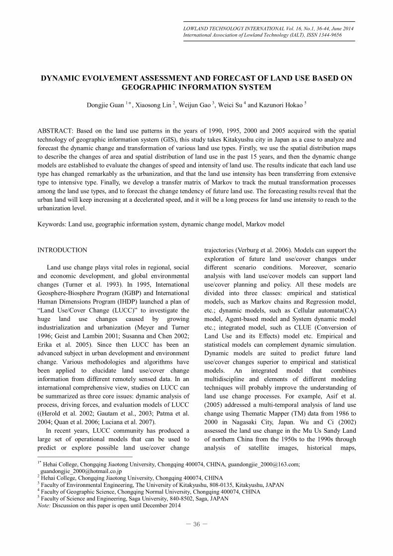
Fig. 1 A map of study area

meteorological, and socioeconomic data. Henk and Latesteijn (1995) studied the land use change based on a Linear Programming model, but the model had no forecast function. Courage (2009) combined physical and socioeconomic data into Markov-CA model to simulate future land use change. However, the model did not successfully forecast the location of bareland class due to the shortage of spatial data. Yu (2009) forecasted future land use change based on Markov-CA model. However, authors did not consider the yearly-changing impact intensity of socio-economic development, policy changes, and other factors on land use change, leading to inaccurate prediction result. Although above three types of models have been recognized by some researchers (Li and Reynolds 1997; Courage et al. 2009), there have been relatively few comprehensive studies to induce the dynamic model to reveal land use change and forecast future change tendency with Markov model.

Dynamic evaluation and forecasting on the future 1and use can essentially reflect how various land use types are continually adjusted to meet the needs of social and economic development. Therefore, research on these issues is conducive to understand the mechanisms of land use change, and to reasonably utilize the land resources in the future through the adjustment of social and economic activities. This study establishes land use patterns in Kitakyushu of Japan and analyzes spatial-temporal changing features from l990 to 2005. Then, transformation speed and intensity change of land use are evaluated by dynamic change model. A transfer matrix of Markov is then used to analyze the transformation process of land use in the different periods, and to simulate the potential change of land use from 2005 to 2020. The purpose is to present a typical research case of revealing land use change during the process of industrialization and urbanization in coastal region. The research results are beneficial to better understand and address a complex land-use system, and to improve the advanced land use management and planning for harmonizing the balanced development between urban expansion and ecological conservation experienced extensively. STUDY AREA

Kitakyushu (33°52'N, 130°49'E) is a city located in

Fukuoka prefecture, Kyushu, Japan. Its total area is 486.81 km2, population is 993,483 till Oct. 2005, and population density is 2040.80 per km2. From the view of topographical features, topographic relief in Kitakyushu is bigger, sea level elevation reaches above 1700 meters, mid-mountain and low-mountain accounting for 35% of

total region area is main topographic types (Fig.1). Kitakyushu borders on the main islands of Japan across Kanmon Strait and is adjacent to several other Asian countries, and particularly it is located at the straight line connecting two largest cities, Tokyo in Japan and Shanghai in China. Meanwhile, the eastern and northern Kitakyushu has a long coast line. It is one of the most active areas in Kyushu and enjoys the fastest economic development. METHODOLOGY Data Source

The data spanned 15 years with four year nodes of 1990, 1995, 2000 and 2005. According to the basic data originated from remote sensing data, topographic map and land use map, Landsat TM images of four different periods were acquired, then images was carried on geometric correction and coordination transformation with ERDAS IMAGE software, and color composites were generated by displaying the bands 5, 4 and 3 as red, green and blue, respectively. Then, an image enhancement of intensifying visual distinction among features was performed to increase the amount of information that could be visually interpreted. In succession, image interpretation symbols of different image elements were added accompanying by field investigations. This could be consulted in the process of person-machine alternating visual operations. Finally, land use type was interpreted visually in the screen based on the TM images, land use spatial database and attribution database were set up, and land use figure of four different years were obtained. For the study purpose, land use were divided into 6 types (agricultural land, forestland, water body, build-up land, public land, and unused land) according to national classification standard of land use and comprehensible ability advisement of TM image, as shown in Table 1. For data

－ 38 －

Dongjie GUAN, et al.

source validation, we compare the data of land use area obtained from TM image with the actual value of land use derived from statistic data of Kitakyushu city. They are basically consistent, so the data source is reliable. DYNAMIC CHANGE ANALYSIS OF LAND USE

Change of Land Use Rate

Dynamic change model of land use, comprised of

single change rate and average change rate of land use, is an important approach to study the land use change. By this model, researchers can analyze speed, process, and development tendency of land use change in the future. Single change rate of land use reflects the change rate of one land use type. Meanwhile, average change rate of land use reflects the mutual transformation speed of all land use types in the different periods (Zhu et al. 2003; Wang and Niu 2006). The two mathematics expressions are listed as follows:

%1001

TUUUK

a

ab (1)

%100

1

1

n

ii

n

iij

U

UE

(2)

where K is the yearly single change rate of a land use type; Ua is the area of a land use type at the beginning year; Ub is the area of a land use type at the ending year; T is the time step (year);E is the average change rate; Ui is the area of land use type i at the beginning year;

is sum of the converted area from the land use type i to the land type j and the converted area from the land use type j to the land use type i in the same period (j ≠ i, j=1, 2…, n).

Change of Land Use Intensity Intensity model of land use is to emphatically study

the synthetic result of intensity change of 1and use type in a studied area. This model can not only reflect the extensity and the intensity of land use, but also depict the change tendency of land use. The index of land use intensity could reflect the change intensity of land use. The change amount of land use intensity and its change rate were used to quantify the composite level and changing trend of land use in the region (Liu and Buheaosier 2000; Turner and Gardner 1991; Wang and Bao 2003; Zhu and Li 2003). According to the different extent of human being’s exploitation and utilization, Liu and Buheaosier (2000) classified the land use intensity into four grades: unused land, extensive land, intensive land, and urban land, as shown in Table 2. The four grades are sequentially expressed as 1, 2, 3, and 4, respectively (if the value is between 1 and 2, intensity grade is categorized as primary level; if the value is between 2 and 3, intensity grade is categorized as middle level; if the value is between 3 and 4, intensity grade is categorized as high level). Because each land use grade contains several land use types (for instance, unused land contains the barren land and the beach), this model can not only reflect the extensity and the intensity of land use, but also depict the change tendency of land use type.

As mentioned above, the index of land use intensity, change amount of land use intensity, and change rate of land use intensity are used to describe the change of land use intensity. The mathematics expressions of the three indices are listed below (Zhu and Li 2003; Hu et al. 2006).

400,100,1001

LCAL i

n

ii 　

(3)

)]()([10011

n

iiaiib

n

iiabab CACALLL

(4)

Table 1 Classified system of land use Land use type General description Agricultural land

Irrigated, level-terraced agricultural lands in river valleys, dry land, vegetable plot

Forestland Forest areas below the 80m elevation, Forest areas and naked rock land above the 80m elevation

Water body River surface, pond surface, lake surface and ditch.

Build-up land Residential land, industrial land, commerce land, road land and public facilities

Public land Road and park Unused land Tidal flat land, barren land, sand

land, grassless land, raised path through fields and others

Table 2 Classifications and grade values of land use intensity Grade Grade Type Land Use Type

1 Unused Land Barren Land, Beaches2 Extensive

Land Forest Land, Water body

3 Intensive Land Cropland, Orchard and Nurseries

4 Urban land Industrial Land, Build-up Land, Road, Commercial Land, Transportation, Utilities

n

1i ijU

－ 39 －


n

iibi

n

i

n

iiaiibi

CA

CACAR

1

1 1

)(

)()(

(5)

where L is the index of 1and use intensity; Ai is the ith grade value of 1and use intensity; Ci is the area percentage of i grade land use intensity; n is the number of grade of land use intensity; Lb is the index of land use intensity at the ending year; La is the index of land use intensity at the beginning year; Cia is the area percentage of i grade land use intensity at the beginning year; Cib is the area percentage of i grade land use intensity at the ending year; R is the change rate of 1and use intensity. If the change amount and the change rate are positive, the 1and use of the region is in a development period; otherwise, it is in a declining period.

Analysis and Forecast with Markov Model

In probability theory and statistics, Markov process is

a time-varying random phenomenon, in which the probability at the future state is only dependent on current state but not on previous ones (Fischer and Sun 2001; Veldkamp and Lambin 2001; Pijanowski et al. 2002). The Markov process is appropriate to evaluate the change of land use type, because dynamic change of land use type also possesses the properties of Markov process under the following preconditions: (a) in a certain area, a land use type may be reversibly transformed into another one; (b) the mutual conversion process between land use types includes many incidents which are difficult to be precisely described by special functions; (c) the transformation of land use type is relatively stable and can be accordant with the requirement of Markov Chain.

In this paper, transformation probability of various land uses was forecast by calculation of theoretic tendency value of land use change on Markov model that was a random process without aftereffect, which effectively made up the deficiencies by applying the total area changes of various lands to explain their change. Therefore, it was appropriate that inter-transforming information of land use was digitized into theoretic tendency value for their comparisons, which overcame the disadvantages that they are unable to be directly compared due to different initial years. Emphatically, only if condition of dynamic changes is relatively stable, Markov model can more accurately reflect dynamic change of land use. Also, if forecast is a long-term process, different interference condition will violate forecast result. Therefore, when employing Markov process, first of all, its application precondition and credibility of forecasting results need be testified by a

large amount of data analysis and evaluation; and then Markov model need be further amended according to essence and requirement of different detailed study cases.

Prior to the use of Markov process, an original probability matrix of transformation of land use type need be defined as follows:

nnnn

n

n

xy

PPP

PPPPPP

PP

......

......

)(

21

22221

11211

(6) In the above matrix, Pxy is the probability for

transformation of the xth land use type into the yth land use type; n is the amount of land use type. Pxy should meet the following requirements:

),...,3,2,1,(10 nyxPxy (7)

),...,3,2,1,(11

nyxPn

xxy

(8)

According to non-aftereffect of Marko v process and probability formulas of Bayes condition, forecast model of Markov is obtained:

xyPnPnP )1()( (9)

where P(n) is the probability of current state; P(n-1) is the probability of previous state.

RESULTS AND DISCUSSIONS

Analysis on Quantity and Spatial Distribution of Land Use

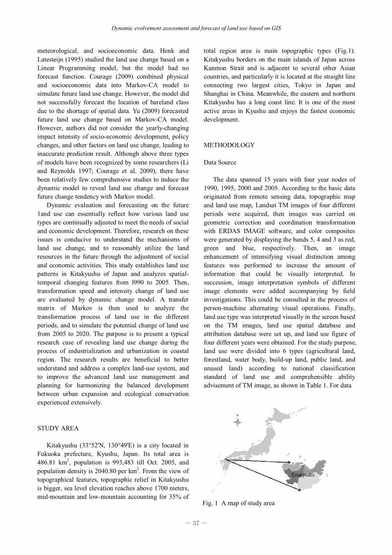
Firstly, the area changes of all land use types at the

years of 1990, 1995, 2000, and 2005, are computed in Fig.2. It is apparent that agricultural land and forestland

Agricultural land Forestland Water body Build-up land Public land Unused land0

50

100

150

200

250

Year

Land

use

are

a(km

2 )

1990 1995 2000 2005

Fig. 2 Area changes of land use types from 1990 to 2005 in Kitakyushu

－ 40 －


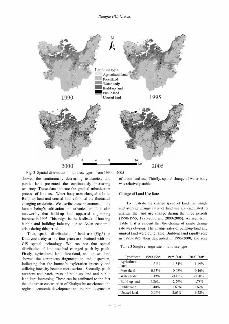
showed the continuously decreasing tendencies, and public land presented the continuously increasing tendency. These data indicate the gradual urbanization process of land use. Water body area changed a little. Build-up land and unused land exhibited the fluctuated changing tendencies. We ascribe these phenomena to the human being’s cultivation and urbanization. It is also noteworthy that build-up land appeared a jumping increase in 1995. This might be the feedback of housing bubble and building industry due to Asian economic crisis during this period.

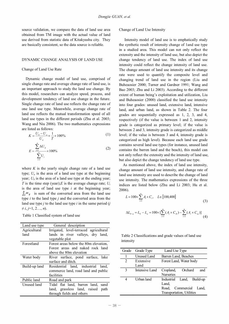
Then, spatial distributions of land use (Fig.3) in Kitakyushu city at the four years are obtained with the GIS spatial technology. We can see that spatial distribution of land use had changed patch by patch. Firstly, agricultural land, forestland, and unused land showed the continuous fragmentation and dispersion, indicating that the human’s exploration intensity and utilizing intensity became more serious. Secondly, patch numbers and patch areas of build-up land and public land kept increasing. These can be attributed to the fact that the urban construction of Kitakyushu accelerated the regional economic development and the rapid expansion

of urban land use. Thirdly, spatial change of water body was relatively stable.

Change of Land Use Rate

To illustrate the change speed of land use, single

and average change rates of land use are calculated to analyze the land use change during the three periods (1990-1995, 1995-2000 and 2000-2005). As seen from Table 3, it is evident that the change of single change rate was obvious. The change rates of build-up land and unused land were quite rapid. Build-up land rapidly rose in 1990-1995, then descended in 1995-2000, and rose

Table 3 Single change rate of land use type

Type/Year 1990-1995 1995-2000 2000-2005 Agricultural land -1.34% -1.54% -1.49%

Forestland -0.13% -0.08% -0.16% Water body 0.39% -0.45% -0.80% Build-up land 4.86% -2.29% 1.78% Public land 0.40% 1.69% 1.62% Unused land -3.64% 2.63% -9.52%

Fig. 3 Spatial distribution of land use types from 1990 to 2005

－ 41 －


slowly in 2000-2005. Whereas, the change rate of unused land was contrary to that of build-up land. The change rate of agricultural land slowly decreased in the three periods. The change rate of public land became quicker. The change rates of forestland and water body were slow. According to Eq.(2), average change rate of land use in the three periods were computed to be 22.9 %, 19.6 %, and 11.7 %, respectively, indicating that the transformation speed of land use decreased from 1990 to 2005. Change of Land Use Intensity

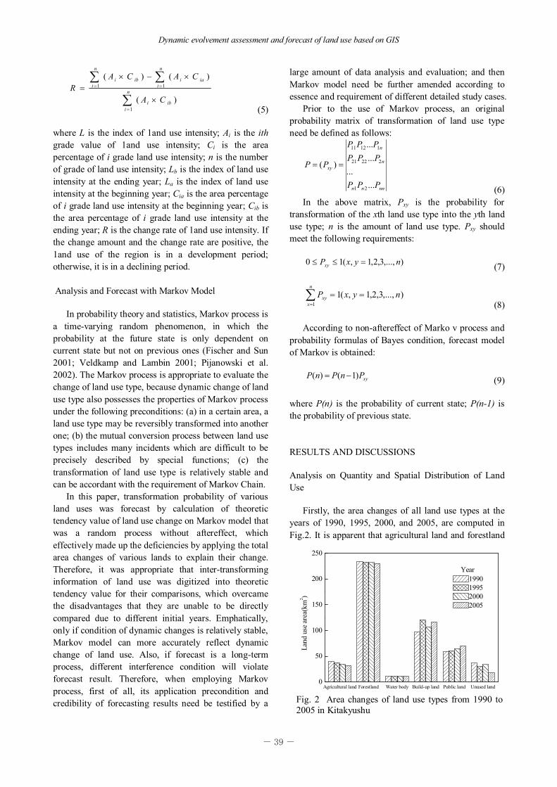
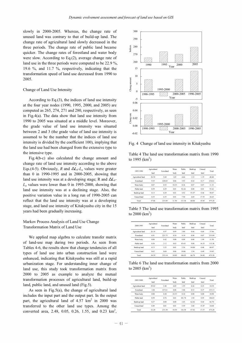
According to Eq.(3), the indices of land use intensity

at the four year nodes (1990, 1995, 2000, and 2005) are computed as 265, 274, 271 and 280, respectively, as seen in Fig.4(a). The data show that land use intensity from 1990 to 2005 was situated at a middle level. Moreover, the grade value of land use intensity was situated between 2 and 3 (the grade value of land use intensity is assumed to be the number that the indices of land use intensity is divided by the coefficient 100), implying that the land use had been changed from the extensive type to the intensive type.

Fig.4(b-c) also calculated the change amount and change rate of land use intensity according to the above Eqs.(4-5). Obviously, R and △Lb-La values were greater than 0 in 1990-1995 and in 2000-2005, showing that land use intensity was at a developing stage; R and △Lb-La values were lower than 0 in 1995-2000, showing that land use intensity was at a declining stage. Also, the positive variation value in a long run of 1990-2005 can reflect that the land use intensity was at a developing stage, and land use intensity of Kitakyushu city in the 15 years had been gradually increasing.

Markov Process Analysis of Land Use Change Transformation Matrix of Land Use

We applied map algebra to calculate transfer matrix

of land-use map during two periods. As seen from Tables 4-6, the results show that change tendencies of all types of land use into urban construction land were enhanced, indicating that Kitakyushu was still at a rapid urbanization stage. For understanding inner change of land use, this study took transformation matrix from 2000 to 2005 as example to analyze the mutual transformation processes of agricultural land, build-up land, public land, and unused land (Fig.5).

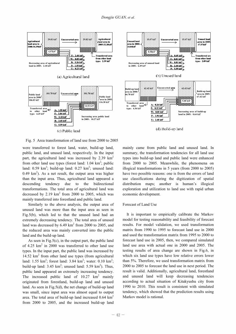
As seen in Fig.5(a), the change of agricultural land includes the input part and the output part. In the output part, the agricultural land of 4.57 km2 in 2000 was transferred to the other land use types. Among the converted area, 2.48, 0.05, 0.26, 1.55, and 0.23 km2,

1990-1995 1995-2000 2000-2005 1990-2005-0.02

0.00

0.02

0.04

0.06

Cha

ng ra

te2000-2005

-5

0

5

10

15 Year

Ch

ang

amou

nt

2005200019951990

1990-2005

1990-20051995-2000

1995-2000

2000-2005

1990-1995

1990-1995

260

270

280

290

300

Year

Year

Indi

ces

Fig. 4 Change of land use intensity in Kitakyushu Table 4 The land use transformation matrix from 1990 to 1995 (km2)

1995/1990 Agricultural

land Forestland

Water

body

Public

land

Build-up

land

Unused

land Total

Agricultural land 26.58 5.60 1.05 4.66 1.32 1.19 40.40

Forestland 9.35 220.65 0.06 3.93 0.44 0.17 234.61

Water body 0.07 0.52 10.35 0.24 0.07 0.07 11.33

Public land 0.59 0.29 0.01 92.44 0.08 0.01 93.42

Build-up land 0.13 0.29 0.01 4.52 53.47 0.46 58.87

Unused land 0.35 6.55 0.01 7.50 4.69 17.55 36.65

Total 37.06 233.89 11.50 113.30 60.08 19.45 475.28

Table 5 The land use transformation matrix from 1995 to 2000 (km2)


land Forestland

Water

body

Public

land

Build-up

land

Unused

land Total


Forestland 6.91 221.73 0.10 4.10 0.98 0.07 233.89

Water body 0.00 0.42 9.00 0.08 0.00 1.99 11.50

Public land 0.56 2.12 0.83 85.65 9.80 14.35 113.30

Build-up land 0.13 3.22 0.01 2.26 54.00 0.46 60.07

Unused land 0.62 0.68 0.06 10.06 1.54 6.49 19.45

Total 34.39 233.14 10.89 106.03 66.78 24.05 475.28

Table 6 The land use transformation matrix from 2000 to 2005 (km2)


land Forestland

Water

body

Public

land

Build-up

land

Unused

land Total


Forestland 1.04 227.61 0.06 3.84 0.32 0.27 233.13

Water body 0.00 0.44 10.35 0.10 0.00 0.00 10.90

Public land 0.59 0.76 0.01 101.78 1.94 0.95 106.03

Build-up land 0.27 0.00 0.00 3.45 62.42 0.64 66.78

Unused land 0.49 0.01 0.01 5.59 2.48 15.47 24.04

Total 32.20 231.30 10.50 116.30 67.42 17.57 475.28

－ 42 －


were transferred to forest land, water, build-up land, public land, and unused land, respectively. In the input part, the agricultural land was increased by 2.39 km2 from other land use types (forest land: 1.04 km2; public land: 0.59 km2; build-up land: 0.27 km2; unused land: 0.49 km2). As a net result, the output area was higher than the input area. Thus, agricultural land appeared a descending tendency due to the bidirectional transformations. The total area of agricultural land was decreased by 2.19 km2 from 2000 to 2005, which was mainly transferred into forestland and public land.

Similarly to the above analysis, the output area of unused land was more than the input area as seen in Fig.5(b), which led to that the unused land had an extremely decreasing tendency. The total area of unused land was decreased by 6.49 km2 from 2000 to 2005, and the reduced area was mainly converted into the public land and the build-up land.

As seen in Fig.5(c), in the output part, the public land of 4.25 km2 in 2000 was transferred to other land use types. In the input part, the public land was increased by 14.52 km2 from other land use types (from agricultural land: 1.55 km2; forest land: 3.84 km2; water: 0.10 km2; build-up land: 3.45 km2; unused land: 5.59 km2). Thus, public land appeared an extremely increasing tendency. The increased public land of 10.27 km2 mainly originated from forestland, build-up land and unused land. As seen in Fig.5(d), the net change of build-up land was small, since input area was almost equal to output area. The total area of build-up land increased 0.64 km2 from 2000 to 2005, and the increased build-up land

mainly came from public land and unused land. In summary, the transformation tendencies for all land use types into build-up land and public land were enhanced from 2000 to 2005. Meanwhile, the phenomena on illogical transformations in 5 years (from 2000 to 2005) have two possible reasons: one is from the errors of land use classifications during the digitization of spatial distribution maps; another is human’s illogical exploration and utilization to land use with rapid urban economic development.

Forecast of Land Use

It is important to empirically calibrate the Markov

model for testing reasonability and feasibility of forecast results. For model validation, we used transformation matrix from 1990 to 1995 to forecast land use in 2000 and used the transformation matrix from 1995 to 2000 to forecast land use in 2005, then, we compared simulated land use area with actual one in 2000 and 2005. The testing results of area change are shown in Fig.6, in which six land use types have low relative errors lower than 5%. Therefore, we used transformation matrix from 2000 to 2005 to forecast the land use in next period. The result is valid. Additionally, agricultural land, forestland and unused land will keep decreasing tendencies according to actual situation of Kitakyushu city from 1990 to 2010. This result is consistent with simulated tendency, which showed that the prediction results using Markov model is rational.

F：2.48 k㎡

29.82 k㎡29.82 k㎡

Decreasing area of agricultural land in 2005：2.18 k㎡

4.57k㎡

W：0.05 k㎡

P：1.55 k㎡U：0.23 k㎡

Transferred area from other land type：2.39 k㎡

Agricultural land area in 2000:34.39k㎡


Unconverted area

B：0.26 k㎡

F：2.48 k㎡

29.82 k㎡29.82 k㎡29.82 k㎡

Decreasing area of agricultural land in 2005：2.18 k㎡

4.57k㎡

W：0.05 k㎡

P：1.55 k㎡U：0.23 k㎡

Transferred area from other land type：2.39 k㎡



Unconverted area

B：0.26 k㎡

A：0.49 k㎡

15.47 k㎡15.47 k㎡

Decreasing area of unused land in 2005：6.49 k㎡

8.58k㎡

F：0.01 k㎡

B：2.48 k㎡P：5.59 k㎡

Transferred arefrom other landtype：2.09 k㎡

Unused land area in 2000:24.04k㎡


Unconverted area

W：0.01 k㎡

A：0.49 k㎡

15.47 k㎡15.47 k㎡

Decreasing area of unused land in 2005：6.49 k㎡

8.58k㎡

F：0.01 k㎡

B：2.48 k㎡P：5.59 k㎡

Transferred arefrom other landtype：2.09 k㎡



Unconverted area

W：0.01 k㎡

(a) Agricultural land (b) Unused land

Transferred area to other land type：4.25 k㎡

A：1.55 k㎡F：3.84 k㎡W：0.10 k㎡B：3.45 k㎡

U：5.59 k㎡

Increasing area public land in 2005：10.27 k㎡

101.78 k㎡ 101.78 k㎡

14.52 k㎡

Public land area in 2000:106.03 k㎡


Unconverted area


A：1.55 k㎡F：3.84 k㎡W：0.10 k㎡B：3.45 k㎡

U：5.59 k㎡

Increasing area public land in 2005：10.27 k㎡

101.78 k㎡ 101.78 k㎡

14.52 k㎡



Unconverted area


A：0.26 k㎡F：0.32 k㎡W：0.00 k㎡

P：1.94 k㎡

U：2.48 k㎡

Increasing area of build-up land in 2005：0.64 k㎡

Build-up land area in 2000:66.78 k㎡

62.42 k㎡ 62.42 k㎡

5.00 k㎡

Unconverted areaBuild-up land area in 2005:

67.42 k㎡


A：0.26 k㎡F：0.32 k㎡W：0.00 k㎡

P：1.94 k㎡

U：2.48 k㎡

Increasing area of build-up land in 2005：0.64 k㎡

Build-up land area in 2000:66.78 k㎡

62.42 k㎡ 62.42 k㎡

5.00 k㎡

Unconverted areaBuild-up land area in 2005:

67.42 k㎡

(c) Public land (d) Build-up land

Fig. 5 Area transformation of land use from 2000 to 2005

－ 43 －


Additionally, land use is influenced by a series of economic, social, natural, artificial factors which are more complicated than our consideration in establishing model. We thus assume that the shorter and closer the period used for the forecast is, more accurate the forecast result is. This paper forecasted land use change for easily understanding the dynamic change tendency in the future. However, if forecast period is too long, accuracy of prediction result is not reliable. If the forecast time is too short, the change tendency is not clear. So, potential land use change are simulated from 2005 to 2020 in Kitakyushu according to the transformation matrix from 2000 to 2005, P (2005) value are calculated using Markov chain model According to Eq.(7-9). Calculation processes of P (n) value from 2010 to 2020 are abbreviated.

3337.0,0792.0,5172.0,0003.0,0349.0,0319.00077.0,8999.0,0376.0,0002.0,0536.0,0023.01266.0,0865.0,9599.0,7559.0,0187.0,0050.01732.0,0000.0,0070.0,7833.0,0366.0,0000.00003.0,0042.0,0175.0,0004.0,9480.0,0295.00184.0,0124.0,1047.0,0240.0,1341.0,7064.0

120.0,242.0,060.0,023.0,479.0,0755.0

( )20001995()2000()2005(

PPP

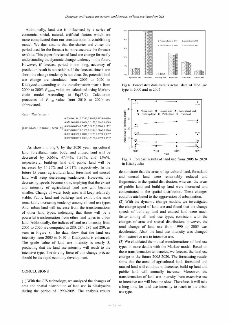
As shown in Fig.7, by the 2020 year, agricultural

land, forestland, water body, and unused land will be decreased by 5.66%, 47.44%, 1.97%, and 1.96%, respectively; build-up land and public land will be increased by 14.26% and 28.71%, respectively. In the future 15 years, agricultural land, forestland and unused land will keep decreasing tendencies. However, the decreasing speeds become slow, implying that the extent and intensity of agricultural land use will become smaller. Change of water body area will keep relatively stable. Public land and build-up land exhibit the most remarkably increasing tendency among all land use types. And, urban land will increase from the transformations of other land types, indicating that there will be a powerful transformation from other land types to urban land. Additionally, the indices of land use intensity from 2005 to 2020 are computed as 280, 284, 287 and 289, as seen in Figure 8. The data show that the land use intensity from 2005 to 2010 in Kitakyushu is enhanced. The grade value of land use intensity is nearly 3, predicting that the land use intensity will reach to the intensive type. The driving force of this change process should be the rapid economy development. CONCLUSIONS

(1) With the GIS technology, we analyzed the changes of area and spatial distribution of land use in Kitakyushu during the period of 1990-2005. The analysis results

demonstrate that the areas of agricultural land, forestland and unused land were remarkably reduced and fragmented in the spatial distribution, whereas, the areas of public land and build-up land were increased and concentrated in the spatial distribution. These changes could be attributed to the aggravation of urbanization. (2) With the dynamic change models, we investigated the change speed of land use and found that the change speeds of build-up land and unused land were much faster among all land use types, consistent with the changes of area and spatial distribution; however, the total change of land use from 1990 to 2005 was decelerated. Also, the land use intensity was changed from extensive use to intensive use. (3) We elucidated the mutual transformations of land use types in more details with the Markov model. Based on these transformation tendencies, we forecast the land use change in the future 2005-2020. The forecasting results show that the areas of agricultural land, forestland and unused land will continue to decrease; build-up land and public land will annually increase. Moreover, the transformation of land use intensity from extensive use to intensive use will become slow. Therefore, it will take a long time for land use intensity to reach to the urban use type.

0%

10%

20%

30%

40%

50%

Agriculture land Forestland Build-up land Public land Water body Unused land

Forecasted data in 2005 Actual data in 2005

Forecasted data in 2000 Actual data in 2000

Fig.6 Forecasted data versus actual data of land use type in 2000 and in 2005

2005 2010 2015 20200

10

20

30

40

50

47.4448.67

28.71

24.47

14.2614.18

5.666.78

1.963.7

1.972.21

Perc

enta

ge o

f lan

d us

e ar

ea(%

)

Year

Water body Unused land Agricultural land Build-up land Public land Forestland

Fig. 7 Forecast results of land use from 2005 to 2020 in Kitakyushu

－ 44 －


ACKNOWLEDGEMENTS The research is supported by National Natural

Scientific Foundation of China (No. 41201546) and Natural Scientific Foundation of Chongqing in China (No. cstc2012jjA20010).

REFERENCES Asif, A., Shaikhl, K. G., Kaoru, T. (2005). Multi-

temporal Analysis of land cover changes in Nagasaki City associated with natural disasters using satellite remote sensing. J. Nat. Disaster Sci., 27: 9-15.

Courage, K., Masamu, A., Bongo, A. and Munyaradzi, M. (2009). Rural sustainability under threat in Zimbabwe-Simulation of future land use/cover changes in the Bindura District based on the Markov-Cellular Automata Model. Appl. Geo., 29: 435-447.

Erika L., Eric, F. and Lambin, A. C. (2005). A synthesis of information on rapid land-cover change for the period 1981-2000. Bioscience, 55: 115-124.

Fischer., G. and Sun, L. X. (2001). Model based analysis of future land-use development in China. Agricul. Ecosys. Environ., 85: 163-176.

Gautam, A. P., Webb, E. L. and Shivakoti, G. P. (2003). Land use dynamics and landscape change pattern in a mountain watershed in Nepa1. Agricul. Ecosys. Environ., 99: 83-96.

Geist, H. J. and Lambin, E. F., (2001). What Drives Tropical Deforestation. LUCC Report Series, 4: 1-2.

Henk, C. and Latesteijn, V. (1995). Assessment of future options for land use in the European Community. Ecol. Engrg., 4: 211-222

Herold, M. J. and Scepan, K., C. (2002). The use of remote sensing and landscape metrics to describe structures and changes in urban land uses. Environ. Plan. A, 34: 1443-1458.

Hu, Z. L.,Du, P. J. And Guo, D. Z. (2006). Analysis of spatio-temporal changes of land use in xuzhou city based on remote sensing. J. China Univ. of Mining and Technology, 16: 151-155.

Li, H. and Reynolds, J.F., (1997). Modeling Effects of Spatial Pattern, Drought, and Grazing on Rates of Rangeland Degradation: A Combined Markov and Cellular Automaton Approach. In D. A. Quattrochi, and M. F. Goodchild (Eds.), Scale in Remote Sensing and GIS. Boca Raton, Florida: Lewis Publish.: 211-230

Liu, J. Y. and Buheaosier (2000). A study on spatial-temporal feature of modem land use change in China: Using remote sensing techniques. Quarter. Sci., 20: 229-235.

Luciana, P. B., Edward, A. E. and Henry, L. G. (2007). Land use dynamics and landscape history in La Montaña, Campeche, Mexico. Lands. Urban Plan., 82: 198-207.

Meyer, W. B. and Turner, B. L., (1996). Land-use/land-cover change: Challenges for geographers. Geo Journal, 39: 237-240.

Patma, V., Sukaesinee, S. and Viriya, L. (2004). From forest to farm fields: Changes in land use in undulating terrain of Northeast Thailand at different scales during the past century. Southeast Asian Studies, 41: 444-472.

Pijanowski, B. C., Brown, D. G. and Shellito, B. A. (2002). Using neural networks and GIS to forecast land use changes: A land transformation model. Computers Environ. Urban Sys., 26: 553-575.

Quan, B. N., Chen, J. F. and Qiu, H. L. (2006). spatial-temporal pattern and driving forces of land use changes in Xiamen. Pedoshere, 16: 477-488.

Susanna, T. Y. and Chen, W. L. (2002). Modeling the relationship between land use and surface water quality. J. Environ. Management, 66: 377-393.

Turner, M. G. and Gardner, R. H. ( 1991). Quantitative Methods in Landscape Ecology. Springer Verlag, New York, U. S. A.: 289-308.

Turner, B. L., Moss R. H. and Skole D. L. (1993). Relating Land Use and Global Land-Cover Change: A Proposal for an IGBP-HDP Core Project. IGBP Report No. 24 HDP Report No.5. Stockholm: Int. Geosphere-Biosphere Programme: 66

Verburg, P. H., de Koning, G. H. J., Kok, K., Veldkamp, A. And Bouma, J. (1999). A Spatial explicit allocation procedure for modelling the pattern of land use change based upon actual land use. Ecol. Model., 116: 45-61.

Veldkamp, A. and Lambin, E. F. (2001). Predicting land-use change. Agricul. Ecosys. Environ., 85: 1-6.

Wang, X. and Bao, Y. (1999). Study on the methods of land use dynamic change research. Progress in Geo., 18(1): 81-87.

Wang, L. and Niu, Z. (2006). Analyzing land use change of small towns based on RS technology. Resource Sci., 28: 68-75.

Wu, B., and Ci, L.J. (2002). Landscape change and desertification development in the Mu US Sandland Northern China. J. Arid Environ., 50: 429-444.

Yu, F. (2009). Study on forecast of land use change based on Markov-CA, Land Res. Information (In Chinese), 4: 38-46.

Zhu, H. Y. and Li, X. B. (2003). Discussion on the index method of regional land use change. Acta Geographica Sinica, 58: 643-650.

Documents

DYNAMIC EVOLVEMENT ASSESSMENT AND …portal.dl.saga-u.ac.jp/bitstream/123456789/122399/1/quan_201406.pdf · technology of geographic information system ... Dynamic evolvement assessment