Embed Size (px)
Citation preview
Dynamic Enforcement of Knowledge-basedSecurity Policies using Probabilistic Abstract
Interpretation
Piotr Mardziel†, Stephen Magill, Michael Hicks†, Mudhakar Srivatsa?
† University of Maryland, College Park? IBM T.J. Watson Research Laboratory
January 24, 2013
Abstract
This paper explores the idea of knowledge-based security policies, which areused to decide whether to answer queries over secret data based on an estima-tion of the querier’s (possibly increased) knowledge given the results. Limitingknowledge is the goal of existing information release policies that employ mech-anisms such as noising, anonymization, and redaction. Knowledge-based policiesare more general: they increase flexibility by not fixing the means to restrict infor-mation flow. We enforce a knowledge-based policy by explicitly tracking a modelof a querier’s belief about secret data, represented as a probability distribution, anddenying any query that could increase knowledge above a given threshold. We im-plement query analysis and belief tracking via abstract interpretation, which allowsus to trade off precision and performance through the use of abstraction. We havedeveloped an approach to augment standard abstract domains to include probabili-ties, and thus define distributions. We focus on developing probabilistic polyhedrain particular, to support numeric programs. While probabilistic abstract interpre-tation has been considered before, our domain is the first whose design supportssound conditioning, which is required to ensure that estimates of a querier’s knowl-edge are accurate. Experiments with our implementation show that several usefulqueries can be handled efficiently, particularly compared to exact (i.e., sound) in-ference involving sampling. We also show that, for our benchmarks, restrictingconstraints to octagons or intervals, rather than full polyhedra, can dramaticallyimprove performance while incurring little to no loss in precision.
1 IntroductionFacebook, Twitter, Flickr, and other successful on-line services enable users to easilyfoster and maintain relationships by sharing information with friends and fans. Theseservices store users’ personal information and use it to customize the user experience
1
and to generate revenue. For example, Facebook third-party applications are grantedaccess to a user’s “basic” data (which includes name, profile picture, gender, networks,user ID, and list of friends [5]) to implement services like birthday announcements andhoroscopes, while Facebook selects ads based on age, gender, and even sexual pref-erence [27]. Unfortunately, once personal information is collected, users have limitedcontrol over how it is used. For example, Facebook’s EULA grants Facebook a non-exclusive license to any content a user posts [2]. MySpace, another social network site,has begun to sell its users’ data [56].
Some researchers have proposed that, to keep tighter control over their data, userscould use a storage server (e.g., running on their home network) that handles personaldata requests, and only responds when a request is deemed safe [50, 8]. The questionis: which requests are safe? While deferring to user-defined access control policiesseems an obvious approach, such policies are unnecessarily restrictive when the goalis to maximize the customized personal experience. To see why, consider two exam-ple applications: a horoscope or “happy birthday” application that operates on birthmonth and day, and a music recommendation algorithm that considers birth year (age).Access control at the granularity of the entire birth date could preclude both of theseapplications, while choosing only to release birth year or birth day precludes accessto one application or the other. But in fact the user may not care much about theseparticular bits of information, but rather about what can be deduced from them. Forexample, it has been reported that zip code, birth date, and gender are sufficient infor-mation to uniquely identify 87% of Americans in the 1990 U.S. census [55] and 63%in the 2000 census [25]. So the user may be perfectly happy to reveal any one of thesebits of information as long as a querier gains no better than a 1/n chance to guess theentire group, for some parameter n.
This paper explores the design and implementation for enforcing what we callknowledge-based security policies. In our model, a user U ’s agent responds to queriesinvolving secret data. For each querying principal Q, the agent maintains a probabilitydistribution over U ’s secret data, representing Q’s belief of the data’s likely values.For example, to mediate queries from a social networking site X , user U ’s agent maymodel X’s otherwise uninformed knowledge of U ’s birthday according to a likely de-mographic: the birth month and day are uniformly distributed, while the birth year ismost likely between 1956 and 1992 [1]. Each querier Q is also assigned a knowledge-based policy, expressed as a set of thresholds, each applying to a different group of(potentially overlapping) data. For example, U ’s policy for X might be a threshold of1/100 for the entire tuple (birthdate, zipcode, gender), and 1/5 for just birth date. U ’sagent refuses any queries that it determines could increase Q’s ability to guess a secretabove the assigned threshold. If deemed safe, U ’s agent returns the query’s (exact)result and updates Q’s modeled belief appropriately.
Throughout the paper we use users’ personal information protection when interact-ing with services like Facebook (or its advertisers) as a running example, but knowledge-based security policies have other applications as well. For example, they can be usedto decide whether a principal should participate in a secure multiparty computation in-volving multiple principals each with its own secrets, such as their current locationor available resources. We have explored this application in some detail in recentwork [34]. Knowledge-based policies could also be used to protect against browser
2
fingerprinting, which aims to uniquely identify individuals based on environmental in-dicators visible to Javascript programs [10]. Users could set a threshold policy overthe tuple of the most sensitive indicators, and prevent the execution of the Javascriptprogram (or execute only a modified version) if the threshold is exceeded. Anotherexample would be application to privacy-preserving smart metering [49]. Here, theproposal is that rather than report fine-grained power usage information back to thepower company, which could compromise privacy, the pricing algorithm is run locallyon the meter, with only the final charge returned. Our work could be combined with thiswork to ensure that knowledge that can be inferred from the output indeed preservesprivacy sufficiently. We elaborate on these and other examples in Section 8.
To implement our model, we need (1) an algorithm to check whether answeringa query could violate a knowledge-based policy, (2) a method for revising a querier’sbelief according to the answer that is given, and (3) means to implement (1) and (2)efficiently. We build on the work of Clarkson et al. [14] (reviewed in Section 3), whichworks out the theoretical basis for (2). The main contributions of this paper, therefore,in addition to the idea of knowledge-based policies, are our solutions to (1) and (3).
Given a means to revise querier beliefs based on prior answers, it seems obvioushow to check that a query does not reveal too much: U runs the query, tentativelyrevisesQ’s belief based on the result, and then responds with the answer only ifQ’s re-vised belief about the secrets does not exceed the prescribed thresholds. Unfortunately,with this approach the decision to accept or reject depends on the actual secret, so a re-jection could leak information. We give an example in the next section that shows howthe entire secret could be revealed. Therefore, we propose that a query should be re-jected if there exists any possible secret value that could induce an output whereby therevised belief would exceed the threshold. This idea is described in detail in Section 4.
The foundational elements of our approach, belief tracking and revision, can beimplemented using languages for probabilistic computation. However, existing lan-guages of this variety—IBAL [45], Church [26], Fun [11], and several other sys-tems [47, 44, 30, 38]— are problematic because they are either unsound or too in-efficient. Systems that use exact inference have no flexibility of approximation to effi-ciently handle large or complex state spaces. Systems that use approximate inferenceare more efficient, but the nature of the approximation is under-specified, and thus thereis no guarantee of soundness.
We have developed an implementation based on abstract interpretation [17] that iscapable of approximate inference, but is sound relative to our policies. In particular,our implementation ensures that, despite the use of abstraction, the probabilities we as-cribe to the querier’s belief are never less than the true probabilities. At the center of ourimplementation is a new abstract domain we call a probabilistic polyhedra, describedin Section 5, which extends the standard convex polyhedron abstract domain [19] withmeasures of probability. We represent beliefs as a set of probabilistic polyhedra (as de-veloped in Section 6). Our approach can easily be adapted to any abstract domain thatsupports certain common operations; our implementation includes support for intervals[16] and octagons [39].
While some prior work has explored probabilistic abstract interpretation [40], thiswork does not support belief revision, which is required to track how observation ofoutputs affects a querier’s belief. Support for revision requires that we maintain both
3
under- and over-approximations of probabilities in the querier’s belief, whereas priorwork deals only with over-approximation. We have developed an implementation ofour approach based on Parma [6], an abstract interpretation library, and LattE [21], atool for counting the integer points contained in a polygon. We discuss the implementa-tion in Section 7 along with some experimental measurements of its performance. Wefind that the varying the number of polyhedra permitted for performing belief trackingconstitutes a useful precision/performance tradeoff, and that reasonable performancecan be had while maintaining good precision.
Knowledge-based policies aim to ensure that an attacker’s knowledge of a secretdoes not increase much when learning the result of a query. Much prior work aims toenforce similar properties by tracking information leakage quantitatively [37, 53, 7, 32,48]. Our approach is more precise (but also more resource-intensive) because it main-tains an on-line model of adversary knowledge. An alternative to knowledge-basedprivacy is differential privacy [24] (DP), which requires that a query over a databaseof individuals’ records produces roughly the same answer whether a particular indi-vidual’s data is in the database or not—the possible knowledge of the querier, and theimpact of the query’s result on it, need not be directly considered. As such, DP avoidsthe danger of mismodeling a querier’s knowledge and as a result inappropriately re-leasing information. DP also need not maintain a per-querier belief representation foranswering subsequent queries. However, DP applies once an individual has releasedhis personal data to a trusted third party’s database, a release we are motivated to avoid.Moreover, applying DP to queries over an individual’s data, rather than a population,introduces so much noise that the results are often useless. We discuss these issuesalong with other related work in Section 9.
A preliminary version of this paper was published at CSF’11 [35]. The presentversion expands the formal description of probabilistic polyhedra and details of theirimplementation, and expands our experimental evaluation. We have refined some defi-nitions to improve performance (e.g., the forget operation in Section 5.3.1) and imple-mented two new abstract domains (Section 5.5). We have also expanded our bench-mark suite to include several additional programs (Section 7.1 and Appendix A). Wediscuss the performance/precision tradeoffs across the different domains/benchmarks(Section 7.3). Proofs, omitted for space reasons, appear in a companion technical re-port [36].
2 OverviewThe next section presents a technical overview of the paper through a running example.Full details of the approach are presented in Sections 3–7.
Knowledge-based policies and beliefs. User Bob would like to enforce a knowledge-based policy on his data so that advertisers do not learn too much about him. SupposeBob considers his birthday of September 27, 1980 to be relatively private; variablebday stores the calendar day (a number between 0 and 364, which for Bob would be270) and byear stores the birth year (which would be 1980). To bday he assigns aknowledge threshold td = 0.2 stating that he does not want an advertiser to have betterthan a 20% likelihood of guessing his birth day. To the pair (bday , byear) he assigns a
4

threshold tdy = 0.05, meaning he does not want an advertiser to be able to guess thecombination of birth day and year together with better than a 5% likelihood.
Bob runs an agent program to answer queries about his data on his behalf. Thisagent models an estimated belief of queriers as a probability distribution δ, which isconceptually a map from secret states to positive real numbers representing probabil-ities (in range [0, 1]). Bob’s secret state is the pair (bday = 270, byear = 1980). Theagent represents a distribution as a set of probabilistic polyhedra. For now, we canthink of a probabilistic polyhedron as a standard convex polyhedron C with a proba-bility mass m, where the probability of each integer point contained in C is m/#(C),where #(C) is the number of integer points contained in the polyhedron C. Shortlywe present a more involved representation.
Initially, the agent might model an advertiser X’s belief using the following rect-angular polyhedron C, where each point contained in it is considered equally likely(m = 1):
C = 0 ≤ bday < 365, 1956 ≤ byear < 1993
An initial belief such as this one could be derived from several sources. For exam-ple, Facebook publishes demographics of its users [1], and similar sorts of personaldemographics could be drawn from census data, surveys, employee records, etc. De-mographics are also relevant to other applications; e.g., initial beliefs for hiding webbrowser footprints can be based on browser surveys, likely movie preferences can befound from IMDB, and so on. In general, we observe that understanding the capabili-ties and knowledge of a potential adversary is necessary no matter the kind of securitypolicy used; often this determination is implicit, rather than explicit as in our approach.We defer further discussion on this topic to Sections 9 and 8.
Enforcing knowledge-based policies safely. Suppose X wants to identify userswhose birthday falls within the next week, to promote a special offer. X sends Bob’sagent the following program.
Example 1.today := 260;if bday ≥ today ∧ bday < (today + 7) thenoutput := True;
This program refers to Bob’s secret variable bday , and also uses non-secret variablestoday , which represents the current day and is here set to be 260, and output , whichis set to True if the user’s birthday is within the next seven days (we assume output isinitially False).
The agent must decide whether returning the result of running this program willpotentially increase X’s knowledge about Bob’s data above the prescribed threshold.We explain how it makes this determination shortly, but for the present we can seethat answering the query is safe: the returned output variable will be False whichessentially teaches the querier that Bob’s birthday is not within the next week, whichstill leaves many possibilities. As such, the agent revises his model of the querier’sbelief to be the following pair of rectangular polyhedra C1, C2, where again all pointsin each are equally likely (with probability masses m1 = 260
358 ≈ 0.726,m2 = 98358 ≈
5

0.274):C1 = 0 ≤ bday < 260, 1956 ≤ byear < 1993C2 = 267 ≤ bday < 365, 1956 ≤ byear < 1993
Ignoring byear , there are 358 possible values for bday and each is equally likely. Thusthe probability of any one is 1/358 ≈ 0.0028 ≤ td = 0.2. More explicitly, the samequantity can be computed using the definition of conditional probability: Pr(A|B) =Pr(A ∧ B)/Pr(B) where event A refers to bday having one particular value (e.g.,not in the next week) and event B refers to the query returning False. Thus 1/358 =
1365/
358365 .
Suppose the next day the same advertiser sends the same program to Bob’s useragent, but with today set to 261. Should the agent run the program? At first glance,doing so seems OK. The program will return False, and the revised belief will be thesame as above but with constraint bday ≥ 267 changed to bday ≥ 268, meaning thereis still only a 1/357 ≈ 0.0028 chance to guess bday .
But suppose Bob’s birth day was actually 267, rather than 270. The first querywould have produced the same revised belief as before, but since the second querywould return True (since bday = 267 < (261 + 7)), the querier can deduce Bob’sbirth day exactly: bday ≥ 267 (from the first query) and bday < 268 (from the secondquery) together imply that bday = 267! But the user agent is now stuck: it cannotsimply refuse to answer the query, because the querier knows that with td = 0.2 (orindeed, any reasonable threshold) the only good reason to refuse is when bday = 267.As such, refusal essentially tells the querier the answer.
The lesson is that the decision to refuse a query must not be based on the effect ofrunning the query on the actual secret, because then a refusal could leak information. InSection 4 we propose that an agent should reject a program if there exists any possiblesecret that could cause a program answer to increase querier knowledge above thethreshold. As such we would reject the second query regardless of whether bday = 270or bday = 267. This makes the policy decision simulatable [29]: given knowledge ofthe current belief model and the belief-tracking implementation being used, the queriercan determine whether his query will be rejected on his own.
Full probabilistic polyhedra. Now suppose, having run the first query and rejectedthe second, the user agent receives the following program from X .
Example 2.
age := 2011− byear ;if age = 20 ∨ age = 30 ∨ ... ∨ age = 60 then output := True;pif 0.1 then output := True;
This program attempts to discover whether this year is a “special” year for the givenuser, who thus deserves a special offer. The program returns True if either the user’sage is (or will be) an exact decade, or if the user wins the luck of the draw (one chancein ten), as implemented by the probabilistic if statement.
Running this program reveals nothing about bday , but does reveal something aboutbyear . In particular, if output = False then the querier knows that byear 6∈ {1991,1981, 1971, 1961}, but all other years are equally likely. We could represent this new
6

259
1956
1962
1972
1982
1992
0 267 ...bday
byea
r
259
1956
1962
1972
1982
1992
0 267 ...bday
byea
r
1991
1981
1971
1961
(a) output = False (b) output = True
Figure 1: Example 2: most precise revised beliefs
knowledge, combined with the knowledge gained from the first query, as shown inFigure 1(a), where each shaded box is a polyhedron containing equally likely points.On the other hand, if output = True then either byear ∈ {1991, 1981, 1971, 1961}or the user got lucky. We represent the querier’s knowledge in this case as in Fig-ure 1(b). Darker shading indicates higher probability; thus, all years are still pos-sible, though some are much more likely than others. With the given threshold oftdy = 0.05, the agent will permit the query; when output = False, the likelihoodof any point in the shaded region is
(910 ∗
137∗358
)/(
910 ∗
3337
)= 1/(33 ∗ 358); when
output = True, the points in the dark bands are the most likely, with probability(1
37∗358
)/(
910 ∗
437 + 1
10
)= 10/(73 ∗ 358) (this and the previous calculation are also
just instantiations of the definition of conditional probability). Since both outcomes arepossible with Bob’s byear = 1980, the revised belief will depend on the result of theprobabilistic if statement.
This example illustrates a potential problem with the simple representation of prob-abilistic polyhedra mentioned earlier: when output = False we will jump from usingtwo probabilistic polyhedra to ten, and when output = True we jump to using eigh-teen. Allowing the number of polyhedra to grow without bound will result in per-formance problems. To address this concern, we need a way to abstract our beliefrepresentation to be more concise.
Section 5 shows how to represent a probabilistic polyhedron P as a seven-tuple,(C, smin, smax,pmin,pmax,mmin,mmax) where smin and smax are lower and upperbounds on the number of points with non-zero probability in the polyhedron C (calledthe support points of C); the quantities pmin and pmax are lower and upper boundson the probability mass per support point; and mmin and mmax give bounds on thetotal probability mass. Thus, polyhedra modeled using the simpler representation(C,m) given earlier are equivalent to ones in the more involved representation withmmax = mmin = m, pmax = pmin = m/#(C), and smax = smin = #(C).
With the seven-tuple representation, we could choose to collapse the sets of polyhe-dra given in Figure 1. For example, we could represent Figure 1(a) with two probabilis-tic polyhedra P1 and P2 containing polyhedra C1 and C2 defined above, respectively,essentially drawing a box around the two groupings of smaller boxes in the figure. The
7
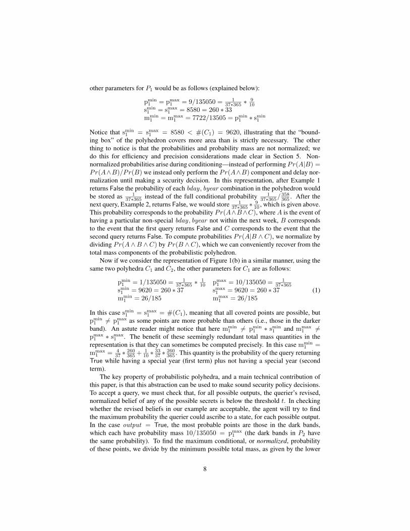
other parameters for P1 would be as follows (explained below):
pmin1 = pmax
1 = 9/135050 = 137∗365 ∗
910
smin1 = smax
1 = 8580 = 260 ∗ 33mmin
1 = mmax1 = 7722/13505 = pmin
1 ∗ smin1
Notice that smin1 = smax
1 = 8580 < #(C1) = 9620, illustrating that the “bound-ing box” of the polyhedron covers more area than is strictly necessary. The otherthing to notice is that the probabilities and probability mass are not normalized; wedo this for efficiency and precision considerations made clear in Section 5. Non-normalized probabilities arise during conditioning—instead of performing Pr(A|B) =Pr(A∧B)/Pr(B) we instead only perform the Pr(A∧B) component and delay nor-malization until making a security decision. In this representation, after Example 1returns False the probability of each bday , byear combination in the polyhedron wouldbe stored as 1
37∗365 instead of the full conditional probability 137∗365/
358365 . After the
next query, Example 2, returns False, we would store 137∗365 ∗
910 , which is given above.
This probability corresponds to the probability Pr(A∧B∧C), whereA is the event ofhaving a particular non-special bday , byear not within the next week, B correspondsto the event that the first query returns False and C corresponds to the event that thesecond query returns False. To compute probabilities Pr(A|B ∧ C), we normalize bydividing Pr(A ∧B ∧C) by Pr(B ∧C), which we can conveniently recover from thetotal mass components of the probabilistic polyhedron.
Now if we consider the representation of Figure 1(b) in a similar manner, using thesame two polyhedra C1 and C2, the other parameters for C1 are as follows:
pmin1 = 1/135050 = 1
37∗365 ∗110 pmax
1 = 10/135050 = 137∗365
smin1 = 9620 = 260 ∗ 37 smax
1 = 9620 = 260 ∗ 37mmin
1 = 26/185 mmax1 = 26/185
(1)
In this case smin1 = smax
1 = #(C1), meaning that all covered points are possible, butpmin
1 6= pmax1 as some points are more probable than others (i.e., those in the darker
band). An astute reader might notice that here mmin1 6= pmin
1 ∗ smin1 and mmax
1 6=pmax
1 ∗ smax1 . The benefit of these seemingly redundant total mass quantities in the
representation is that they can sometimes be computed precisely. In this case mmin1 =
mmax1 = 4
37 ∗260365 + 1
10 ∗3337 ∗
260365 . This quantity is the probability of the query returning
True while having a special year (first term) plus not having a special year (secondterm).
The key property of probabilistic polyhedra, and a main technical contribution ofthis paper, is that this abstraction can be used to make sound security policy decisions.To accept a query, we must check that, for all possible outputs, the querier’s revised,normalized belief of any of the possible secrets is below the threshold t. In checkingwhether the revised beliefs in our example are acceptable, the agent will try to findthe maximum probability the querier could ascribe to a state, for each possible output.In the case output = True, the most probable points are those in the dark bands,which each have probability mass 10/135050 = pmax
1 (the dark bands in P2 havethe same probability). To find the maximum conditional, or normalized, probabilityof these points, we divide by the minimum possible total mass, as given by the lower
8
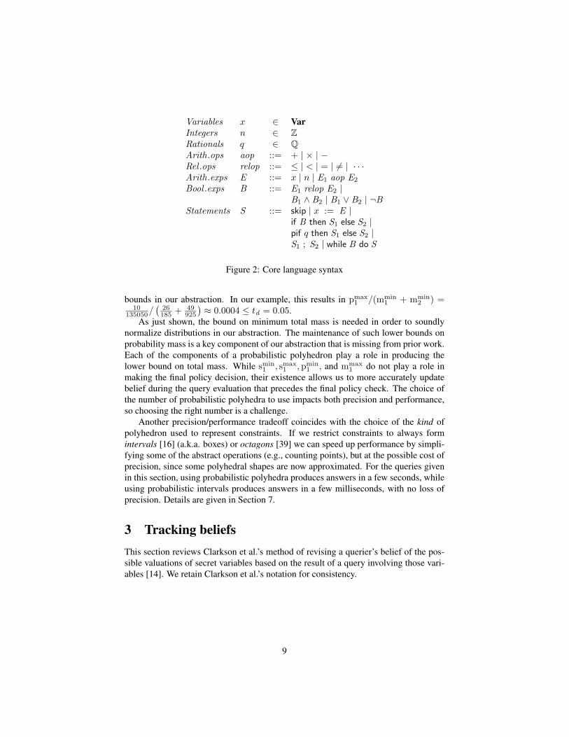
Variables x ∈ VarIntegers n ∈ ZRationals q ∈ QArith.ops aop ::= + | × | −Rel .ops relop ::= ≤ | < | = | 6= | · · ·Arith.exps E ::= x | n | E1 aop E2
Bool .exps B ::= E1 relop E2 |B1 ∧ B2 | B1 ∨ B2 | ¬B
Statements S ::= skip | x := E |if B then S1 else S2 |pif q then S1 else S2 |S1 ; S2 | while B do S
Figure 2: Core language syntax
bounds in our abstraction. In our example, this results in pmax1 /(mmin
1 + mmin2 ) =
10135050/
(26185 + 49
925
)≈ 0.0004 ≤ td = 0.05.
As just shown, the bound on minimum total mass is needed in order to soundlynormalize distributions in our abstraction. The maintenance of such lower bounds onprobability mass is a key component of our abstraction that is missing from prior work.Each of the components of a probabilistic polyhedron play a role in producing thelower bound on total mass. While smin
1 , smax1 ,pmin
1 , and mmax1 do not play a role in
making the final policy decision, their existence allows us to more accurately updatebelief during the query evaluation that precedes the final policy check. The choice ofthe number of probabilistic polyhedra to use impacts both precision and performance,so choosing the right number is a challenge.
Another precision/performance tradeoff coincides with the choice of the kind ofpolyhedron used to represent constraints. If we restrict constraints to always formintervals [16] (a.k.a. boxes) or octagons [39] we can speed up performance by simpli-fying some of the abstract operations (e.g., counting points), but at the possible cost ofprecision, since some polyhedral shapes are now approximated. For the queries givenin this section, using probabilistic polyhedra produces answers in a few seconds, whileusing probabilistic intervals produces answers in a few milliseconds, with no loss ofprecision. Details are given in Section 7.
3 Tracking beliefsThis section reviews Clarkson et al.’s method of revising a querier’s belief of the pos-sible valuations of secret variables based on the result of a query involving those vari-ables [14]. We retain Clarkson et al.’s notation for consistency.
9

3.1 Core languageThe programming language we use for queries is given in Figure 2. A computationis defined by a statement S whose standard semantics can be viewed as a relationbetween states: given an input state σ, running the program will produce an outputstate σ′. States are maps from variables to integers:
σ, τ ∈ State def= Var→ Z
Sometimes we consider states with domains restricted to a subset of variables V , inwhich case we write σV ∈ StateV
def= V → Z. We may also project states to a set of
variables V :σ � V
def= λx ∈ VarV . σ(x)
The language is essentially standard, though we limit the form of expressions to supportour abstract interpretation-based semantics (Section 5). The semantics of the statementform pif q then S1 else S2 is non-deterministic: the result is that of S1 with probabilityq, and S2 with probability 1− q.
Note that in our language, variables have only integer values and the syntax ismissing a division operator. Furthermore, we will restrict arithmetic expressions to beof a linear forms only, that is, multiplication of two variables will be disallowed. Theserestrictions ease implementation considerations. Easing these constraints is an aspectof our future work.
3.2 Probabilistic semantics for tracking beliefsTo enforce a knowledge-based policy, an agent must be able to estimate what a queriercould learn from the output of his query. To do this, the agent keeps a distributionδ that represents the querier’s belief of the likely valuations of the user’s secrets. Adistribution is a map from states to positive real numbers, interpreted as probabilities(in range [0, 1]).
δ ∈ Dist def= State→ R+
We sometimes focus our attention on distributions over states of a fixed set of variablesV , in which case we write δV ∈ DistV to mean a function StateV → R+. Thevariables of a state, written fv(σ) is defined by domain(σ), sometimes we will refer tothis set as just the domain of σ. We will also use the this notation for distributions;fv(δ)
def= domain(domain(δ)). In the context of distributions, domain will also refer to
the set fv(δ) as opposed to domain(δ).Projecting distributions onto a set of variables is as follows:1
δ � Vdef= λσV ∈ StateV .
∑τ : τ�V=σV
δ(τ)
We will often project away a single variable. We will call this operation forget.Intuitively the distribution forgets about a variable x.
fx(δ)def= δ � (fv(δ)− {x})
1The notation∑x : π ρ can be read ρ is the sum over all x such that formula π is satisfied (where x is
bound in ρ and π).
10
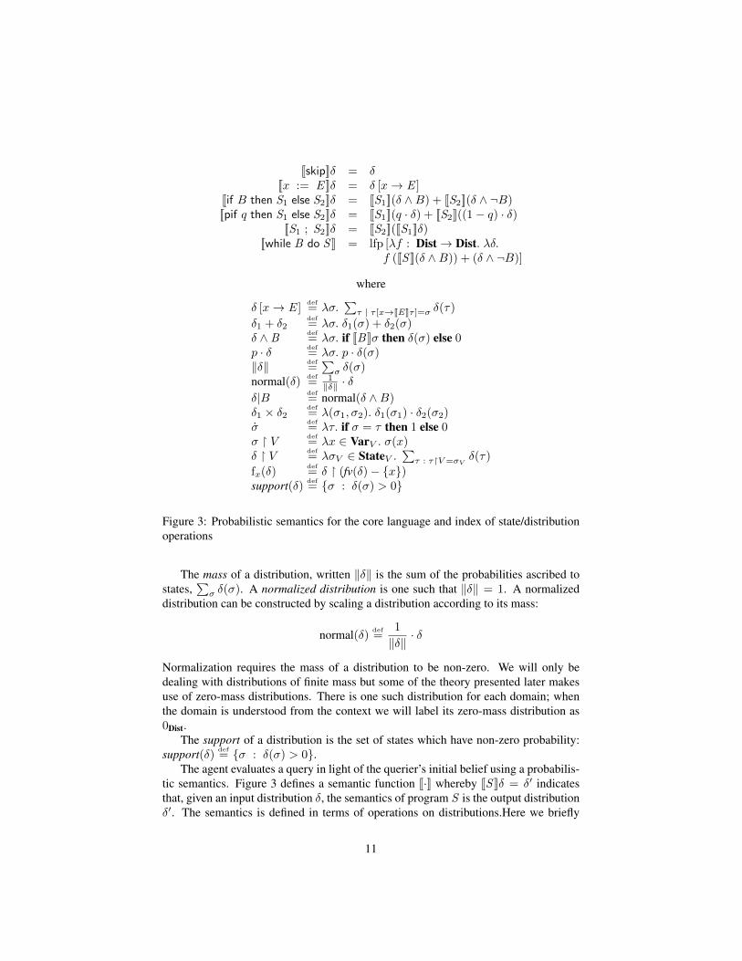
[[skip]]δ = δ[[x := E ]]δ = δ [x→ E ]
[[if B then S1 else S2]]δ = [[S1]](δ ∧B) + [[S2]](δ ∧ ¬B)[[pif q then S1 else S2]]δ = [[S1]](q · δ) + [[S2]]((1− q) · δ)
[[S1 ; S2]]δ = [[S2]]([[S1]]δ)[[while B do S ]] = lfp [λf : Dist→ Dist. λδ.
f ([[S ]](δ ∧B)) + (δ ∧ ¬B)]
where
δ [x→ E ]def= λσ.
∑τ | τ [x→[[E ]]τ ]=σ δ(τ)
δ1 + δ2def= λσ. δ1(σ) + δ2(σ)
δ ∧ Bdef= λσ. if [[B ]]σ then δ(σ) else 0
p · δ def= λσ. p · δ(σ)
‖δ‖ def=∑σ δ(σ)
normal(δ) def= 1‖δ‖ · δ
δ|B def= normal(δ ∧B)
δ1 × δ2def= λ(σ1, σ2). δ1(σ1) · δ2(σ2)
σdef= λτ. if σ = τ then 1 else 0
σ � Vdef= λx ∈ VarV . σ(x)
δ � Vdef= λσV ∈ StateV .
∑τ : τ�V=σV
δ(τ)
fx(δ)def= δ � (fv(δ)− {x})
support(δ) def= {σ : δ(σ) > 0}
Figure 3: Probabilistic semantics for the core language and index of state/distributionoperations
The mass of a distribution, written ‖δ‖ is the sum of the probabilities ascribed tostates,
∑σ δ(σ). A normalized distribution is one such that ‖δ‖ = 1. A normalized
distribution can be constructed by scaling a distribution according to its mass:
normal(δ) def=
1
‖δ‖· δ
Normalization requires the mass of a distribution to be non-zero. We will only bedealing with distributions of finite mass but some of the theory presented later makesuse of zero-mass distributions. There is one such distribution for each domain; whenthe domain is understood from the context we will label its zero-mass distribution as0Dist.
The support of a distribution is the set of states which have non-zero probability:support(δ) def
= {σ : δ(σ) > 0}.The agent evaluates a query in light of the querier’s initial belief using a probabilis-
tic semantics. Figure 3 defines a semantic function [[·]] whereby [[S ]]δ = δ′ indicatesthat, given an input distribution δ, the semantics of program S is the output distributionδ′. The semantics is defined in terms of operations on distributions.Here we briefly
11
explain the concrete probabilistic semantics.The semantics of skip is straightforward: it is the identity on distributions. The
semantics of sequences S1 ; S2 is also straightforward: the distribution that resultsfrom executing S1 with δ is given as input to S2 to produce the result.
The semantics of assignment is δ [x→ E ], which is defined as follows:
δ [x→ E ]def= λσ.
∑τ | τ [x→[[E ]]τ ]=σ
δ(τ)
In other words, the result of substituting an expression E for x is a distribution wherestate σ is given a probability that is the sum of the probabilities of all states τ that areequal to σ when x is mapped to the distribution on E in τ .
The semantics for conditionals makes use of two operators on distributions whichwe now define. First, given distributions δ1 and δ2 we define the distribution sum asfollows:
δ1 + δ2def= λσ. δ1(σ) + δ2(σ)
In other words, the probability mass for a given state σ of the summed distribution isjust the sum of the masses from the input distributions for σ. Second, given a distri-bution δ and a boolean expression B , we define the distribution conditioned on B tobe
δ ∧ Bdef= λσ. if [[B ]]σ then δ(σ) else 0
In short, the resulting distribution retains only the probability mass from δ for states σin which B holds.
With these two operators, the semantics of conditionals can be stated simply: theresulting distribution is the sum of the distributions of the two branches, where thefirst branch’s distribution is conditioned on B being true, while the second branch’sdistribution is conditioned on B being false.
The semantics for probabilistic conditionals is like that of conditionals but makesuse of distribution scaling, which is defined as follows: given δ and some scalar p in[0, 1], we have
p · δ def= λσ. p · δ(σ)
In short, the probability ascribed to each state is just the probability ascribed to thatstate by δ but multiplied by p. For probabilistic conditionals, we sum the distributionsof the two branches, scaling them according to the odds q and 1− q.
The semantics of a single while-loop iteration is essentially that of if B then S else skip;the semantics of the entire loop is the fixed point of a function that composes thedistributions produced by each iteration. That such a fixed point exists is proved byClarkson et al. [14]. For an implementation, however, the evaluation of a loop canbe performed naively, by repeatedly evaluating the loop body until the mass of δ ∧ Bbecomes zero. This process has a chance of diverging, signifying an infinite loop onsome σ ∈ support(δ).
In Section 5 we make use of an additional convenience statement, uniform x n1 n2
(equivalent to a series of probabilistic conditionals) intended to assign a uniform valuein the range {n1, ..., n2} to the variable x.
12
[[uniform x n1 n2]]δ = fx(δ)× δ′
Here we use the distribution product operator, which is defined for two distributionswith disjoint domains (sharing no variables):
δ1 × δ2def= λ(σ1, σ2). δ1(σ1) · δ2(σ2)
The notation (σ1, σ2) is the “concatenation” of two states with disjoint domains. In thedefinition of uniform x n1 n2, δ′ is defined over just the variable x (removed from δby the forget operator) as follows.
δ′ = λσ. if n1 ≤ σ(x) ≤ n2 then1
n2 − n1 + 1else 0
3.3 Belief and securityClarkson et al. [14] describe how a belief about possible values of a secret, expressedas a probability distribution, can be revised according to an experiment using the actualsecret. Such an experiment works as follows.
The values of the set of secret variables H are given by the hidden state σH . Theattacker’s initial belief as to the possible values of σH is represented as a distributionδH . A query is a program S that makes use of variables H and possibly other, non-secret variables from a set L; the final values of L, after running S, are made visibleto the attacker. Let σL be an arbitrary initial state of these variables. Then we take thefollowing steps:
Step 1. Evaluate S probabilistically using the querier’s belief about the secret toproduce an output distribution δ′, which amounts to the attacker’s prediction of thepossible output states. This is computed as δ′ = [[S]]δ, where δ, a distribution overvariables H ∪ L, is defined as δ = δH × σL. Here we write σ to denote the pointdistribution for which only σ is possible:
σdef= λτ. if σ = τ then 1 else 0
Thus, the initial distribution δ is the attacker’s belief about the secret variables com-bined with an arbitrary valuation of the public variables.
Step 2. Using the actual secret σH , evaluate S “concretely” to produce an outputstate σL, in three steps. First, we have δ′ = [[S]]δ, where δ = σH×σL. Second, we haveσ ∈ Γ(δ′) where Γ is a sampling operator that produces a state σ from the domain ofa distribution δ with probability normal(δ)(σ). Finally, we extract the attacker-visibleoutput of the sampled state by projecting away the high variables: σL = σ � L. Thesampling here is needed because S may include probabilistic if statements, and so δ′may not be a point distribution.
Step 3. Revise the attacker’s initial belief δH according to the observed outputσL, yielding a new belief δH = (δ′ ∧ σL) � H . Here, δ′ is conditioned on the out-put σL, which yields a new distribution, and this distribution is then projected to thevariables H . The conditioned distribution δH is the non-normalized representation of
13
the attacker’s belief about the secret variables, after observing the final values of lowvariables. In can be turned into a true distribution by normalizing it.
Note that this protocol assumes that S always terminates and does not modify thesecret state. The latter assumption can be eliminated by essentially making a copyof the state before running the program, while eliminating the former depends on theobserver’s ability to detect nontermination [14].
4 Enforcing knowledge-based policiesWhen presented with a query over a user’s data σH , the user’s agent should only answerthe query if doing so will not reveal too much information. More precisely, given aquery S, the agent will return the public output σL resulting from running S on σHif the agent deems that from this output the querier cannot know the secret state σHbeyond some level of doubt, identified by a threshold t. If this threshold could beexceeded, then the agent declines to run S. We call this security check knowledgethreshold security.
Definition 3 (Knowledge Threshold Security). Let δ′ = [[S]]δ, where δ is the modelof the querier’s initial belief. Then query S is threshold secure iff for all σL ∈support(δ′ � L) and all σ′H ∈ StateH we have (δ′|σL � H)(σ′H) ≤ t.
This definition can be related to the experiment protocol defined in Section 3.3.First, δ′ in the definition is the same as δ′ computed in the first step of the protocol.Step 2 in the protocol produces a concrete output σL based on executing S on the actualsecret σH , and Step 3 revises the querier’s belief based on this output. Definition 3generalizes these two steps: instead of considering a single concrete output based onthe actual secret it considers all possible concrete outputs, as given by support(δ′ � L),and ensures that the revised belief in each case for all possible secret states must assignprobability no greater than t.
This definition considers a threshold for the whole secret state σH . As described inSection 2 we can also enforce thresholds over portions of a secret state. In particular, athreshold that applies only to variables V ⊆ H requires that all σ′V ∈ StateV result in(δ′|σL � V )(σ′V ) ≤ t.
The two “foralls” in the definition are critical for ensuring security. The reasonwas shown by the first example in Section 2: If we used the flawed approach of justrunning the experiment protocol and checking if δH(σH) > t then rejection dependson the value of the secret state and could reveal information about it. The more generalpolicy ∀σL ∈ support(δ′ � L). (δ′|σL � H)(σH) ≤ t, would sidestep the problem inthe example, but this policy could still reveal information because it too depends on theactual secret σH .
Definition 3 avoids any inadvertent information leakage because rejection is notbased on the actual secret: if there exists any secret such that a possible output wouldreveal too much, the query is rejected. Definition 3 is equivalent to a worst-case condi-tional vulnerability (upper) bound or alternatively a worst-case conditional min-entropy(lower) bound. Min-entropy measures the expected likelihood of an adversary guess-ing the secret value [53]; the stronger worst-case used in our definition does away with
14
expectation and bounds this likelihood regardless of what the secret is. Such worst-case measures were considered in [31] as a means of providing a stronger securityguarantee. In our case, however, the extra strength is a side-effect of our need for asimulatable policy. See Section 9 for further details.
5 Belief revision via abstract interpretationConsider how we might implement belief tracking and revision to enforce the thresholdsecurity property given in Definition 3. A natural choice would be to evaluate queriesusing a probabilistic programming language with support for conditioning, of whichthere are many [45, 47, 44, 26, 30, 12, 38, 11]. Such languages are largely ineffectivefor use in ensuring security guarantees. Approximate inference in these languagescannot ensure security guarantees, while exact inference, due to its lack of abstractionfacilities, can be too inefficient when the state space is large.
We have developed a new means to perform probabilistic computation based onabstract interpretation. In this approach, execution time depends on the complexity ofthe query rather than the size of the input space. In the next two sections, we presenttwo abstract domains. This section presents the first, denoted P, where an abstractelement is a single probabilistic polyhedron, which is a convex polyhedron [19] withinformation about the probabilities of its points.
Because using a single polyhedron will accumulate imprecision after multiple queries,in our implementation we actually use a different domain, denoted Pn (P), for whichan abstract element consists of a set of at most n probabilistic polyhedra (whose con-struction is inspired by powersets of polyhedra [9, 46]). This domain, described in thenext section, allows us to retain precision at the cost of increased execution time. Byadjusting n, the user can trade off efficiency and precision. An important element ofour approach is the ability to soundly evaluate the knowledge-threshold policies, evenunder approximate inference.
5.1 PolyhedraWe first review convex polyhedra, a common technique for representing sets of programstates. We use the meta-variables β, β1, β2, etc. to denote linear inequalities. We writefv(β) to be the set of variables occurring in β; we also extend this to sets, writingfv({β1, . . . , βn}) for fv(β1) ∪ . . . ∪ fv(βn).
Definition 4. A convex polyhedron C = (B, V ) is a set of linear inequalities B ={β1, . . . , βm}, interpreted conjunctively, over dimensions V . We write C for the setof all convex polyhedra. A polyhedron C represents a set of states, denoted γC(C), asfollows, where σ |= β indicates that the state σ satisfies the inequality β.
γC((B, V ))def= {σ : fv(σ) = V, ∀β ∈ B. σ |= β}
Naturally we require that fv({β1, . . . , βn}) ⊆ V . We write fv((B, V )) to denotethe set of variables V of a polyhedron.
15

Given a state σ and an ordering on the variables in fv(σ), we can view σ as apoint in an N -dimensional space, where N = |fv(σ)|. The set γC(C) can then beviewed as the integer-valued lattice points in anN -dimensional polyhedron. Due to thiscorrespondence, we use the words point and state interchangeably. We will sometimeswrite linear equalities x = f(~y) as an abbreviation for the pair of inequalities x ≤ f(~y)and x ≥ f(~y).
Let C = (B, V ). Convex polyhedra support the following operations.
• Polyhedron size, or #(C), is the number of integer points in the polyhedron,i.e., |γC(C)|. We will always consider bounded polyhedra when determiningtheir size, ensuring that #(C) is finite.
• (Logical) expression evaluation, 〈〈B〉〉C returns a convex polyhedron containingat least the points inC that satisfy B . Note thatB may or may not have disjuncts.
• Expression count, C#B returns an upper bound on the number of integer pointsin C that satisfy B . Note that this may be more precise than #(〈〈B〉〉C) if B hasdisjuncts.
• Meet, C1 uC C2 is the convex polyhedron containing exactly the set of points inthe intersection of γC(C1), γC(C2).
• Join, C1 tC C2 is the smallest convex polyhedron containing both γ(C1) andγ(C2).
• Comparison, C1 vC C2 is a partial order whereby C1 vC C2 if and only ifγC(C1) ⊆ γC(C2).
• Affine transform, C [x→ E ], where x ∈ fv(C), computes an affine transforma-tion of C. This scales the dimension corresponding to x by the coefficient of xin E and shifts the polyhedron. For example, ({x ≤ y, y = 2z}, V ) [y → z + y]evaluates to ({x ≤ y − z, y − z = 2z}, V ).
• Forget, fx(C), projects away x. That is, fx(C) = πfv(C)−{x}(C), where πV (C)is a polyhedron C ′ such that γC(C ′) = {σ : τ ∈ γC(C) ∧ σ = τ � V }. SoC ′ = fx(C) implies x 6∈ fv(C ′). The projection of C to variables V , writtenC � V is defined as the forgetting of all the dimensions of C other than V .
• Linear partition CA ↘↙ CB of two (possibly overlapping) polyhedra CA, CB isa set of equivalent disjoint polyhedra {Ci}ni=1. That is, ∪iγC(Ci) = γC(CA) ∪γC(CB) and γC(Ci) ∩ γC(Cj) = ∅ for i 6= j. When CA and CB do not overlapthen CA ↘↙ CB = {CA, CB}.
We write isempty(C) iff γC(C) = ∅.
5.2 Probabilistic PolyhedraWe take this standard representation of sets of program states and extend it to a repre-sentation for sets of distributions over program states. We define probabilistic polyhe-dra, the core element of our abstract domain, as follows.
16
Definition 5. A probabilistic polyhedronP is a tuple (C, smin, smax,pmin, pmax,mmin,mmax). We write P for the set of probabilistic polyhedra. The quantities smin and smax
are lower and upper bounds on the number of support points in the polyhedron C. Thequantities pmin and pmax are lower and upper bounds on the probability mass per sup-port point. The mmin and mmax components give bounds on the total probability mass.Thus P represents the set of distributions γP(P) defined below.
γP(P)def= {δ : support(δ) ⊆ γC(C) ∧
smin ≤ |support(δ)| ≤ smax ∧mmin ≤ ‖δ‖ ≤ mmax∧∀σ ∈ support(δ). pmin ≤ δ(σ) ≤ pmax}
We will write fv(P)def= fv(C) to denote the set of variables used in the probabilistic
polyhedron.
Note the set γP(P) is a singleton exactly when smin = smax = #(C) and pmin =pmax, and mmin = mmax. In such a case γP(P) contains only the uniform distributionwhere each state in γC(C) has probability pmin. In general, however, the concretiza-tion of a probabilistic polyhedron will have an infinite number of distributions. Forexample, the pair of probabilistic polyhedra in Section 2, Equation 1 admits an in-finite set of distributions, with per-point probabilities varied somewhere in the rangepmin
1 and pmax1 . The representation of the non-uniform distribution in that example is
thus approximate, but the security policy can still be checked via the pmax1 (and mmax
2 )properties of the probabilistic polyhedron.
Distributions represented by a probabilistic polyhedron are not necessarily normal-ized (as was true in Section 3.2). In general, there is a relationship between pmin, smin,and mmin, in that mmin ≥ pmin · smin (and mmax ≤ pmax · smax), and the combinationof the three can yield more information than any two in isolation.
Our convention will be to use C1, smin1 , smax
1 , etc. for the components associatedwith probabilistic polyhedron P1 and to use subscripts to name different probabilisticpolyhedra.
Ordering. Distributions are ordered point-wise [14]. That is, δ1 ≤ δ2 if and onlyif ∀σ. δ1(σ) ≤ δ2(σ). For our abstract domain, we say that P1 vP P2 if and only if∀δ1 ∈ γP(P1). ∃δ2 ∈ γP(P2). δ1 ≤ δ2. Testing P1 vP P2 mechanically is non-trivial,but is unnecessary in our semantics. Rather, we need to test whether a distributionrepresents only the zero distribution 0Dist
def= λσ.0 in order to see that a fixed point for
evaluating 〈〈while B do S 〉〉P has been reached. Intuitively, no further iterations of theloop need to be considered once the probability mass flowing into the nth iteration iszero. This condition can be detected as follows:
iszero(P)def=(
smin = smax = 0 ∧mmin = 0 ≤ mmax)
∨(mmin = mmax = 0 ∧ smin = 0 ≤ smax
)∨(isempty(C) ∧ smin = 0 ≤ smax ∧mmin = 0 ≤ mmax
)∨(pmin = pmax = 0 ∧ smin = 0 ≤ smax ∧mmin = 0 ≤ mmax
)
17
If iszero(P) holds, it is the case that γP(P) = {0Dist}. This definition distinguishesγP(P) = ∅ (if P has inconsistent constraints) from γP(P) = {0Dist}. Note that hav-ing a more conservative definition of iszero(P) (which holds for fewer probabilisticpolyhedra P) would simply mean our analysis would terminate less often than it could,with no effect on security.
Following standard abstract interpretation terminology, we will refer to P (Dist)(sets of distributions) as the concrete domain, P as the abstract domain, and γP : P→P (Dist) as the concretization function for P.
5.3 Abstract Semantics for PTo support execution in the abstract domain just defined, we need to provide abstractimplementations of the basic operations of assignment, conditioning, addition, andscaling used in the concrete semantics given in Figure 3. We will overload notationand use the same syntax for the abstract operators as we did for the concrete operators.
As we present each operation, we will also state the associated soundness theo-rem which shows that the abstract operation is an over-approximation of the concreteoperation. Proofs are given in a separate technical report [36].
The abstract program semantics is then exactly the semantics from Figure 3, butmaking use of the abstract operations defined here, rather than the operations on distri-butions defined in Section 3.2. We will write 〈〈S〉〉P to denote the result of executing Susing the abstract semantics. The main soundness theorem we obtain is the following.
Theorem 6. For all P, δ, if δ ∈ γP(P) and 〈〈S〉〉P terminates, then [[S]]δ terminatesand [[S]]δ ∈ γP(〈〈S〉〉P).
When we say [[S]]δ terminates (or 〈〈S〉〉P terminates) we mean that only a finitenumber of loop iterations are required to interpret the statement on a particular dis-tribution (or probabilistic polyhedron). In the concrete semantics, termination can bechecked by iterating until the mass of δ ∧B (where B is a guard) becomes zero. (Notethat [[S]]δ is always defined, even for infinite loops, as the least fixed-point is alwaysdefined, but we need to distinguish terminating from non-terminating loops for secu-rity reasons, as per the comment at the end of Section 3.3.) To check termination in theabstract semantics, we check that upper bound on the mass of P ∧ B becomes zero.In a standard abstract domain, termination of the fixed point computation for loops isoften ensured by use of a widening operator. This allows abstract fixed points to becomputed in fewer iterations and also permits analysis of loops that may not terminate.In our setting, however, non-termination may reveal information about secret values.As such, we would like to reject queries that may be non-terminating.
We enforce this by not introducing a widening operator [19, 15]. Our abstractinterpretation then has the property that it will not terminate if a loop in the querymay be non-terminating (and, since it is an over-approximate analysis, it may also failto terminate even for some terminating computations). We then reject all queries forwhich our analysis fails to terminate in some predefined amount of time. Loops do notplay a major role in any of our examples, and so this approach has proved sufficientso far. We leave for future work the development of a widening operator that soundlyaccounts for non-termination behavior.
18
The proof for Theorem 6 is a structural induction on S; the meat of the proof is inthe soundness of the various abstract operations. The following sections present theseabstract operations and their soundness relative to the concrete operations. The basicstructure of all the arguments is the same: the abstract operation over-approximates theconcrete one.
5.3.1 Forget
We first describe the abstract forget operator fy(P1), which is used in implementingassignment. Our abstract implementation of the operation must be sound relative to theconcrete one, specifically, if δ ∈ γP(P) then fy(δ) ∈ γP(fy(P)).
The concrete forget operation projects away a single dimension:
fx(δ)def= δ � (fv(δ)− {x})
= λσV ∈ StateV .∑
τ : τ�V=σV
δ(τ) where V = fv(δ)− {x}
When we forget variable y, we collapse any states that are equivalent up to the value ofy into a single state.
To do this soundly, we must find an upper bound hmaxy and a lower bound hmin
y onthe number of integer points in C1 that share the value of the remaining dimensions(this may be visualized of as the min and max height of C1 in the y dimension). Moreprecisely, if V = fv(C1) − {y}, then for every σV ∈ γC(C1 � V ) we have hmin
y ≤|{σ ∈ γC(C1) : σ � V = σV }| ≤ hmax
y . Once these values are obtained, we have thatfy(P1)
def= P2 where the following hold of P2.
C2 = fy(C1)
pmin2 = pmin
1 ·max{
hminy − (#(C1)− smin
1 ), 1}
pmax2 = pmax
1 ·min{
hmaxy , smax
1
}smin2 = dsmin
1 /hmaxy e mmin
2 = mmin1
smax2 = min {#(fy(C1)), smax
1 } mmax2 = mmax
1
The new values for the under and over-approximations of the various parametersare derived by reasoning about the situations in which these quantities could be thesmallest or the greatest, respectively, over all possible δ2 ∈ γP(P2) where δ2 = fy(δ1),δ1 ∈ γP(P1). We summarize the reasoning behind the calculations below:
• pmin2 : The minimum probability per support point is derived by considering a
point of P2 that had the least amount of mass of P1 mapped to it. Let us call thispoint σV and the set of points mapped to it S = {σ ∈ γC(C1) : σ � V = σV }.S could have as little as hmin
y points, as per definition of hminy and not all of these
points must be mass-carrying. There are at least smin1 mass-carrying points inC1.
If we assume that as many as possible of the mass carrying points in the regionC1 are outside of S, it must be that S still contains at least hmin
y −(#(C1)−smin1 )
mass carrying-points, each having probability at least pmin1 .
19

Figure 4: Example of a forget operation in the abstract domain P. In this case, hminy = 1
and hmaxy = 3. Note that hmax
y is precise while hminy is an under-approximation. If
smin1 = smax
1 = 9 then we have smin2 = 3, smax
2 = 4, pmin2 = pmin
1 · 1, pmax2 = pmax
2 · 4.
• pmax2 : The maximum number of points of P1 that get mapped to a single point inP2 cannot exceed smax
1 , the number of support points in P1. Likewise it cannotexceed hmax
y as per definition of hmaxy .
• smin2 : There cannot be more than hmax
y support points of P1 that map to a singlepoint in P2 and there are at least smin
1 support points in P1. If we assume thatevery single support point of P2 had the maximum number of points mapped toit, there would still be dsmin
1 /hmaxy e distinct support points in P2.
• smax2 : The maximum number of support points cannot exceed the size of the
region defining P2. It also cannot exceed the number of support points of P1,even if we assumed there was a one-to-one mapping between the support pointsof P1 and support points of P2.
Figure 4 gives an example of a forget operation and illustrates the quantities hmaxy
and hminy . If C1 = (B1, V1), the upper bound hmax
y can be found by maximizing y− y′subject to the constraints B1 ∪ B1[y′/y], where y′ is a fresh variable and B1[y′/y]represents the set of constraints obtained by substituting y′ for y in B1. As our pointsare integer-valued, this is an integer linear programming problem (and can be solvedby ILP solvers). A less precise upper bound can be found by simply taking the extentof the polyhedron C1 along y, which is given by #(πy(C1)).
For the lower bound, it is always sound to use hminy = 1. A more precise estimate
can be obtained by treating the convex polyhedron as a subset of Rn and finding thevertex with minimal height along dimension y. Call this distance u. An example ofthis quantity is labeled hmin
y in Figure 4. Since the shape is convex, all other points willhave y height greater than or equal to u. We then find the smallest number of integerpoints that can be covered by a line segment of length u. This is given by due − 1.The final under-approximation is then taken to be the larger of 1 and due − 1. As thismethod requires us to inspect every vertex of the convex polyhedron and to computethe y height of the polyhedron at that vertex, we can also look for the one upon which
20
the polyhedron has the greatest height, providing us with the estimate for hmaxy .
Lemma 7. If δ ∈ γP(P) then fy(δ) ∈ γP(fy(P)).
We can define an abstract version of projection using forget:
Definition 8. Let f{x1,x2,...,xn}(P) = f{x2,...,xn}(fx1(P)). ThenP � V ′ = f(fv(P)−V ′)(P).
That is, in order to project onto the set of variables V ′, we forget all variables notin V ′.
5.3.2 Assignment
The concrete assignment operation is defined so that the probability of a state σ is theaccumulated probability mass of all states τ that lead to σ via the assignment:
δ [x→ E ]def= λσ.
∑τ : τ [x→[[E ]]τ ]=σ
δ(τ)
The abstract implementation of this operation strongly depends on the invertibilityof the assignment. Intuitively, the set {τ : τ [x→ [[E ]]τ ] = σ} can be obtained fromσ by inverting the assignment, if invertible.2 Otherwise, the set can be obtained byforgetting about the x variable in σ.
Similarly, we have two cases for abstract assignment. If x := E is invertible,the result of the assignment P1 [x→ E] is the probabilistic polyhedron P2 such thatC2 = C1 [x→ E] and all other components are unchanged. If the assignment is notinvertible, then information about the previous value of x is lost. In this case, we forgetx thereby projecting (or “flattening”) onto the other dimensions. Then we introducedimension x back and add a constraint on x that is defined by the assignment. Moreprecisely the process is as follows. Let P2 = fx(P1) where C2 = (B2, V2). ThenP1 [x→ E] is the probabilistic polyhedron P3 with C3 = (B2 ∪ {x = E} , V2 ∪ {x})and all other components as in P2.
The test for invertibility itself is simple as our system restricts arithmetic expres-sions to linear ones. Invertibility relative to a variable x is then equivalent to the pres-ence of a non-zero coefficient given to x in the expression on the right-hand-side of theassignment. For example, x := 42x+ 17y is invertible but x := 17y is not.
Lemma 9. If δ ∈ γP(P) then δ [v → E ] ∈ γP(P [v → E ]).
The soundness of assignment relies on the fact that our language of expressionsdoes not include division. An invariant of our representation is that smax ≤ #(C).When E contains only multiplication and addition the above rules preserve this invari-ant; an E containing division would violate it. Division would collapse multiple pointsto one and so could be handled similarly to projection.
2An assignment x := E is invertible if there exists an inverse function f : State → State suchthat f ([[x := E]]σ) = σ for all σ. Note that the f here needs not be expressible as an assignment inour (integer-based) language, and generally would not be as most integers have no integer multiplicativeinverses.
21
5.3.3 Plus
The concrete plus operation adds together the mass of two distributions:
δ1 + δ2def= λσ. δ1(σ) + δ2(σ)
The abstract counterpart needs to over-approximate this semantics. Specifically, ifδ1 ∈ γP(P1) and δ2 ∈ γP(P2) then δ1 + δ2 ∈ γP(P1 + P2).
The abstract sum of two probabilistic polyhedra can be easily defined if their sup-port regions do not overlap. In such situations, we would define P3 as below:
C3 = C1 tC C2
pmin3 = min
{pmin
1 ,pmin2
}pmax
3 = max {pmax1 ,pmax
2 }smin3 = smin
1 + smin2
smax3 = smax
1 + smax2
mmin3 = mmin
1 + mmin2
mmax3 = mmax
1 + mmax2
If there is overlap between C1 and C2, the situation becomes more complex. Tosoundly compute the effect of plus we need to determine the minimum and maximumnumber of points in the intersection that may be support points for both P1 and for P2.We refer to these counts as the pessimistic overlap and optimistic overlap, respectively,and define them below.
Definition 10. Given two distributions δ1, δ2, we refer to the set of states that are inthe support of both δ1 and δ2 as the overlap of δ1, δ2. The pessimistic overlap of P1
and P2, denoted P1 / P2, is the cardinality of the smallest possible overlap for anydistributions δ1 ∈ γP(P1) and δ2 ∈ γP(P2). The optimistic overlap P1 , P2 is thecardinality of the largest possible overlap. Formally, we define these as follows. .
P1 / P2def= max
{smin1 + smin
2 −(
#(C1) + #(C2)−#(C1 uC C2)), 0}
P1 , P2def= min
{smax1 , smax
2 ,#(C1 uC C2)}
The pessimistic overlap is derived from the usual inclusion-exclusion principle:|A ∩B| = |A|+ |B| − |A ∪B|. The optimistic overlap is trivial; it cannot exceed thesupport size of either distribution or the size of the intersection.
We can now define abstract addition.
Definition 11. If not iszero(P1) and not iszero(P2) then P1 + P2 is the probabilistic
22

polyhedron P3 = (C3, smin3 , smax
3 ,pmin3 ,pmax
3 ) defined as follows.
C3 = C1 tC C2
pmin3 =
{pmin
1 + pmin2 if P1 / P2 = #(C3)
min{
pmin1 ,pmin
2
}otherwise
pmax3 =
{pmax
1 + pmax2 if P1 , P2 > 0
max {pmax1 ,pmax
2 } otherwise
smin3 = max
{smin1 + smin
2 − P1 , P2, 0}
smax3 = min {smax
1 + smax2 − P1 / P2, #(C3)}
mmin3 = mmin
1 + mmin2 | mmax
3 = mmax1 + mmax
2
If iszero(P1) then we define P1 + P2 as identical to P2; if iszero(P2), the sum isdefined as identical to P1.
Lemma 12. If δ1 ∈ γP(P1) and δ2 ∈ γP(P2) then δ1 + δ2 ∈ γP(P1 + P2).
5.3.4 Product
The concrete product operation merges two distributions over distinct variables into acompound distribution over the union of the variables:
δ1 × δ2def= λ(σ1, σ2). δ1(σ1) · δ2(σ2)
When evaluating the product P3 = P1×P2, we assume that the domains of P1 andP2 are disjoint, i.e., C1 and C2 refer to disjoint sets of variables. If C1 = (B1, V1) andC2 = (B2, V2), then the polyhedron C1 × C2
def= (B1 ∪B2, V1 ∪ V2) is the Cartesian
product of C1 and C2 and contains all those states σ for which σ � V1 ∈ γC(C1) andσ � V2 ∈ γC(C2). Determining the remaining components is straightforward since P1
and P2 are disjoint.
C3 = C1 × C2
pmin3 = pmin
1 · pmin2 pmax
3 = pmax1 · pmax
2
smin3 = smin
1 · smin2 smax
3 = smax1 · smax
2
mmin3 = mmin
1 ·mmin2 mmax
3 = mmax1 ·mmax
2
Lemma 13. For all P1, P2 such that fv(P1) ∩ fv(P2) = ∅, if δ1 ∈ γP(P1) and δ2 ∈γP(P2) then δ1 × δ2 ∈ γP(P1 × P2).
In our examples we often find it useful to express uniformly distributed data di-rectly, rather than encoding it using pif. In particular, we extend statements S to in-clude the statement of the form uniform x n1 n2 whose semantics is to define variablex as having a value uniformly distributed between n1 and n2.
〈〈uniform x n1 n2〉〉P1 = fx(P1)× P2
23
Here, P2 has pmin2 = pmax
2 = 1n2−n1+1 , smin
2 = smax2 = n2−n1 +1, mmin
2 = mmax2 =
1, and C2 = ({x ≥ n1, x ≤ n2} , {x}).We will say that the abstract semantics correspond to the concrete semantics of
uniform defined similarly as follows.
[[uniform x n1 n2]]δ = (δ � fv(δ)− {x})× δ2
where δ2 = (λσ.if n1 ≤ σ(x) ≤ n2 then 1n2−n1+1 else 0).
The soundness of the abstract semantics follows immediately from the soundnessof forget and product.
5.3.5 Conditioning
The concrete conditioning operation restricts a distribution to a region defined by aboolean expression, nullifying any probability mass outside it:
δ ∧ Bdef= λσ. if [[B ]]σ then δ(σ) else 0
Distribution conditioning for probabilistic polyhedra serves the same role as meetin the classic domain of polyhedra in that each is used to perform abstract evaluationof a conditional expression in its respective domain.
Definition 14. Consider the probabilistic polyhedron P1 and Boolean expression B .Let n, n be such that n = C1#B and n = C1#(¬B). The value n is an over-approximation of the number of points in C1 that satisfy the condition B and n is anover-approximation of the number of points in C1 that do not satisfy B . Then P1 ∧ Bis the probabilistic polyhedron P2 defined as follows.
pmin2 = pmin
1 smin2 = max
{smin1 − n, 0
}pmax
2 = pmax1 smax
2 = min {smax1 , n}
mmin2 = max
{pmin
2 · smin2 , mmin
1 − pmax1 ·min {smax
1 , n}}
mmax2 = min
{pmax
2 · smax2 , mmax
1 − pmin1 ·max
{smin1 − n, 0
}}C2 = 〈〈B〉〉C1
The maximal and minimal probability per point are unchanged, as conditioningsimply retains points from the original distribution. To compute the minimal numberof points in P2, we assume that as many points as possible from C1 fall in the regionsatisfying ¬B . The maximal number of points is obtained by assuming that a maximalnumber of points fall within the region satisfying B .
The total mass calculations are more complicated. There are two possible ap-proaches to computing mmin
2 and mmax2 . The bound mmin
2 can never be less thanpmin
2 · smin2 , and so we can always safely choose this as the value of mmin
2 . Simi-larly, we can always choose pmax
2 · smax2 as the value of mmax
2 . However, if mmin1 and
mmax1 give good bounds on total mass (i.e., mmin
1 is much higher than pmin1 · smin
1 anddually for mmax
1 ), then it can be advantageous to reason starting from these bounds.We can obtain a sound value for mmin
2 by considering the case where a maximalamount of mass from C1 fails to satisfy B. To do this, we compute n = C1#¬B ,
24

Figure 5: Example of distribution conditioning in the abstract domain P.
which provides an over-approximation of the number of points within C1 but outsidethe area satisfying B. We bound n by smax
1 and then assign each of these points maxi-mal mass pmax
1 , and subtract this from mmin1 , the previous lower bound on total mass.
By similar reasoning, we can compute mmax2 by assuming a minimal amount of
mass m is removed by conditioning, and subtracting m from mmax1 . This m is given
by considering an under-approximation of the number of points falling outside the areaof overlap between C1 andB and assigning each point minimal mass as given by pmin
1 .This m is given by max
(smin1 − n, 0
).
Figure 5 demonstrates the components that affect the conditioning operation. Thefigure depicts the integer-valued points present in two polyhedra—one representingC1 and the other representing B (shaded). As the set of points in C1 satisfying B isconvex, this region is precisely represented by 〈〈B〉〉C1. By contrast, the set of pointsin C1 that satisfy ¬B is not convex, and thus 〈〈¬B〉〉C1 is an over-approximation. Theicons beside the main image indicate which shapes correspond to which componentsand the numbers within the icons give the total count of points within those shapes.
Suppose the components of P1 are as follows.
smin1 = 19 pmin
1 = 0.01 mmin1 = 0.85
smax1 = 20 pmax
1 = 0.05 mmax1 = 0.9
Then n = 4 and n = 16. Note that we have set n to be the number of points in the non-shaded region of Figure 5. This is more precise than the count given by #(〈〈B〉〉C),which would yield 18. This demonstrates why it is worthwhile to have a separateoperation for counting points satisfying a boolean expression. These values of n and ngive us the following for the first four numeric components of P2.
smin2 = max(19− 16, 0) = 3 pmin
2 = 0.01smax2 = min(20, 4) = 4 pmax
2 = 0.05
For the mmin2 and mmax
2 , we have the following for the method of calculation based onp
min/max2 and s
min/max2 .
mmin2 = 0.01 · 3 = 0.03 mmax
2 = 0.05 · 4 = 0.2
For the method of computation based on mmin/max1 , we have
mmin2 = 0.85− 0.05 · 16 = 0.05
mmax2 = 0.9− 0.01 · (19− 4) = 0.75
25

In this case, the calculation based on subtracting from total mass provides a tighterestimate for mmin
2 , while the method based on multiplying pmax2 and smax
2 is better formmax
2 .
Lemma 15. If δ ∈ γP(P) then δ ∧B ∈ γP(P ∧B).
5.3.6 Scalar Product
The scalar product is straightforward both in the concrete and abstract sense; it justscales the mass per point and total mass:
p · δ def= λσ. p · δ(σ)
Definition 16. Given a scalar p in (0, 1], we write p·P1 for the probabilistic polyhedronP2 specified below.
smin2 = smin
1 pmin2 = p · pmin
1
smax2 = smax
1 pmax2 = p · pmax
1
mmin2 = p ·mmin
1 C2 = C1
mmax2 = p ·mmax
1
If p = 0 then p · P2 is defined instead as below:
smin2 = 0 pmin
2 = 0smax2 = 0 pmax
2 = 0mmin
2 = 0 C2 = 0Cmmax
2 = 0
Here 0C refers to a convex polyhedra (over the same dimensions as C2) whoseconcretization is empty.
Lemma 17. If δ1 ∈ γP(P1) then p · δ1 ∈ γP(p · P1).
5.3.7 Normalization
The normalization of a distribution produces a true probability distribution, whose totalmass is equal to 1:
normal(δ) def=
1
‖δ‖· δ
If a probabilistic polyhedron P has mmin = 1 and mmax = 1 then it represents anormalized distribution. We define below an abstract counterpart to distribution nor-malization, capable of transforming an arbitrary probabilistic polyhedron into one con-taining only normalized distributions.
Definition 18. Whenever mmin1 > 0, we write normal(P1) for the probabilistic poly-
hedron P2 specified below.
pmin2 = pmin
1 /mmax1 smin
2 = smin1
pmax2 = pmax
1 /mmin1 smax
2 = smax1
mmin2 = mmax
2 = 1 C2 = C1
26

When mmin1 = 0, we set pmax
2 = 1. Note that if P1 is the zero distribution thennormal(P1) is not defined.
The normalization operator illustrates the key novelty of our definition of proba-bilistic polyhedron: to ensure that the overapproximation of a state’s probability (pmax)is sound, we must divide by the underapproximation of the total probability mass(mmin).
Lemma 19. If δ1 ∈ γP(P1) and normal(δ1) is defined, then normal(δ1) ∈ γP(normal(P1)).
5.4 Policy EvaluationHere we show how to implement the threshold test given as Definition 3 using proba-bilistic polyhedra. To make the definition simpler, let us first introduce a bit of notation.
Notation 20. If P is a probabilistic polyhedron over variables V , and σ is a state overvariables V ′ ⊆ V , then P ∧ σ def
= P ∧ B where B =∧x∈V ′ x = σ(x).
Recall that we define δ|B in the concrete semantics to be normal(δ ∧ B). Thecorresponding operation in the abstract semantics is similar: P|B def
= normal(P ∧ B).
Definition 21. Given some probabilistic polyhedron P1 and statement S, with lowsecurity variables L and high security variables H , where 〈〈S〉〉P1 terminates, let P2 =〈〈S〉〉P1 and P3 = P2 � L. If, for every σL ∈ γC(C3) with ¬iszero(P2 ∧ σL), we haveP4 = (P2|σL) � H with pmax
4 ≤ t, then we write tsecuret(S, P1).
The computation of P3 involves only abstract interpretation and projection, whichare computable using the operations defined previously in this section. If we have asmall number of outputs (as for the binary outputs considered in our examples), we canenumerate them and check ¬iszero(P2∧σL) for each output σL. When this holds (thatis, the output is feasible), we compute P4, which again simply involves the abstract op-erations defined previously. The final threshold check is then performed by comparingpmax
4 to the probability threshold t.Now we state the main soundness theorem for abstract interpretation using prob-
abilistic polyhedra. This theorem states that the abstract interpretation just describedcan be used to soundly determine whether to accept a query.
Theorem 22. Let δ be an attacker’s initial belief. If δ ∈ γP(P1) and tsecuret(S, P1),then S is threshold secure for threshold t when evaluated with initial belief δ.
The proof of this theorem follows from the soundness of the abstraction (Theorem6), noting the direct parallels of threshold security definitions for distributions (Defini-tions 3) and probabilistic polyhedra (Definition 21).
5.5 Supporting Other Domains, Including Intervals and OctagonsOur approach to constructing probabilistic polyhedra from normal polyhedra can beadapted to add probabilities any other abstract domain for which the operations definedin Section 5.1 can be implemented. Most of the operations listed there are standard to
27
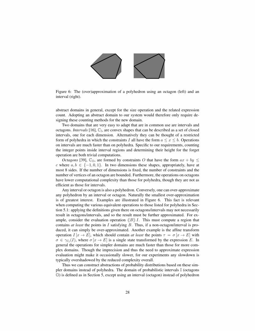
Figure 6: The (over)approximation of a polyhedron using an octagon (left) and aninterval (right).
abstract domains in general, except for the size operation and the related expressioncount. Adopting an abstract domain to our system would therefore only require de-signing these counting methods for the new domain.
Two domains that are very easy to adapt that are in common use are intervals andoctagons. Intervals [16], CI, are convex shapes that can be described as a set of closedintervals, one for each dimension. Alternatively they can be thought of a restrictedform of polyhedra in which the constraints I all have the form a ≤ x ≤ b. Operationson intervals are much faster than on polyhedra. Specific to our requirements, countingthe integer points inside interval regions and determining their height for the forgetoperation are both trivial computations.
Octagons [39], CO, are formed by constraints O that have the form ax + by ≤c where a, b ∈ {−1, 0, 1}. In two dimensions these shapes, appropriately, have atmost 8 sides. If the number of dimensions is fixed, the number of constraints and thenumber of vertices of an octagon are bounded. Furthermore, the operations on octagonshave lower computational complexity than those for polyhedra, though they are not asefficient as those for intervals.
Any interval or octagon is also a polyhedron. Conversely, one can over-approximateany polyhedron by an interval or octagon. Naturally the smallest over-approximationis of greatest interest. Examples are illustrated in Figure 6. This fact is relevantwhen computing the various equivalent operations to those listed for polyhedra in Sec-tion 5.1: applying the definitions given there on octagons/intervals may not necessarilyresult in octagons/intervals, and so the result must be further approximated. For ex-ample, consider the evaluation operation 〈〈B〉〉 I . This must compute a region thatcontains at least the points in I satisfying B . Thus, if a non-octagon/interval is pro-duced, it can simply be over-approximated. Another example is the affine transformoperation I [x→ E ], which should contain at least the points τ = σ [x→ E ] withσ ∈ γCI(I), where σ [x→ E ] is a single state transformed by the expression E . Ingeneral the operations for simpler domains are much faster than those for more com-plex domains. Though the imprecision and thus the need to approximate expressionevaluation might make it occasionally slower, for our experiments any slowdown istypically overshadowed by the reduced complexity overall.
Thus we can construct abstractions of probability distributions based on these sim-pler domains instead of polyhedra. The domain of probabilistic intervals I (octagonsO) is defined as in Section 5, except using an interval (octagon) instead of polyhedron
28

for the region constraint. The abstract semantics described in this section can then besoundly implemented in terms of these simpler shapes in place of polyhedra.
Remark 23. If δ ∈ γP(P) then δ ∈ γI(I) and δ ∈ γO(O), where I and O are identicalto P except P has region constrained by C, a convex polyhedron, while I is con-strained by interval CI and O is constrained by octagon CO, with γC(C) ⊆ γCI(CI)and γC(C) ⊆ γCO(CO).
6 Powerset of Probabilistic PolyhedraThis section presents the Pn (P) domain, an extension of the P domain that abstractlyrepresents a set of distributions as at most n probabilistic polyhedra, elements of P.
Definition 24. A probabilistic (polyhedral) set ∆ is a set of probabilistic polyhedra, or{Pi} with each Pi over the same variables.3 We write Pn (P) for the domain of proba-bilistic polyhedral powersets composed of no more than n probabilistic polyhedra.
Each probabilistic polyhedron P is interpreted disjunctively: it characterizes one ofmany possible distributions. The probabilistic polyhedral set is interpreted additively.To define this idea precisely, we first define a lifting of + to sets of distributions. LetD1, D2 be two sets of distributions. We then define addition as follows.
D1 +D2 = {δ1 + δ2 : δ1 ∈ D1 ∧ δ2 ∈ D2}
This operation is commutative and associative and thus we can use∑
for summationswithout ambiguity as to the order of operations. The concretization function for Pn (P)is then defined as:
γPn(P)(∆)def=∑P∈∆
γP(P)
Following Monniaux’s formulation of a finite sums abstraction [41], elements of ∆need not be disjoint. While enforcing disjointness would simplify determining the mostprobable points for policy evaluation (see Section 6.2), it would necessitate splitting ofprobabilistic polyhedra when overlaps arise. Repeated splitting of already approximateprobabilistic polyhedra decreases their precision and can hurt performance by increas-ing the number of regions to track during abstract interpretation.
We can characterize the condition of ∆ containing only the zero distribution, writ-ten iszero(∆), via the condition that all of the member probabilistic polyhedra arezero.
iszero(∆)def=∧P∈∆
iszero(P)
6.1 Abstract Semantics for Pn (P)The semantics for the powerset abstraction we describe in this section is designed tosoundly approximate the concrete semantics.
3We write {Xi} as shorthand for a set of n elements of type X , for some n. We write {Xi}ni=1 whenthe choice of n is important.
29
Theorem 25. For all δ, S,∆, if δ ∈ γPn(P)(∆) and 〈〈S〉〉∆ terminates, then [[S]]δterminates and [[S]]δ ∈ γPn(P)(〈〈S〉〉∆).
The proof for this theorem follows the same form as the corresponding soundnesstheorem for probabilistic polyhedra (Theorem 6), via soundness of the individual ab-stract operations in relation to their concrete versions. The full proof of this is given inthe companion technical report [36].
To bound the size of the set of probabilistic polyhedra that will arise from thevarious operations that will follow, we introduce a simplification operation.
Definition 26. The powerset simplification transforms a set containing potentiallymore than n elements into one containing no more than n, for n ≥ 1. The simplestapproach involves repeated use of abstract plus in the base domain P.
b{Pi}mi=1cndef=
{{Pi}mi=1 if m ≤ n
b{Pi}m−2i=1 ∪ {Pm−1 + Pm}cn otherwise
Lemma 27. γPn(P)(∆) ⊆ γPn(P)(b∆cm) where m ≤ n.
Note that the order in which individual probabilistic polyhedra are simplified hasno effect on soundness but may impact the precision of the resulting abstraction. Weexplore the variation in precision due to these choices in Section 7.3.
Many of the operations and lemmas for the powerset domain are simple liftingsof the corresponding operations and lemmas for single probabilistic polyhedra. Forthese operations (the first four, below) we simply list the definition; we elaborate onthe remaining four.
Forget fy(∆)def= {fy(P) : P ∈ ∆}
Project. ∆ � Vdef= {P � V : P ∈ ∆}
Assignment. ∆ [x→ E]def= {P [x→ E] : P ∈ ∆}
Scalar product. p ·∆ def= {p · P : P ∈ ∆ ∧ ¬iszero(p · P)}
Conditioning Recall that for probabilistic polyhedra, conditioning P ∧ B is definedin terms of logical expression evaluation for convex polyhedra, 〈〈B〉〉C. This operationreturns a convex polyhedron that contains at least the points in C that satisfy the logicalexpression B . This operation is tight if B does not contain disjuncts. When B doeshave disjuncts whose union does not define a convex region then the operation will beapproximate. Consider Example 2. The condition age = 20 ∨ age = 30 ∨ ... ∨ age =60, were it be approximated using a single convex region, would be equivalent to thecondition age ≥ 20 ∨ age ≤ 60.
In the powerset domain we keep track of multiple convex regions hence can betterapproximate the conditioning operation. The approach we take is to convert the logicalexpression into a disjoint disjunctive normal form: ddnf (B)
def= {B1, B2, · · · , Bm},
such that {σ : σ |= B} = {σ : σ |= B1 ∨ · · · ∨ Bm}, each disjunct Bi contains nofurther disjunctions, and {σ : σ |= Bi ∧ Bj} = ∅ for all i 6= j (Bi are disjoint).
30
Conditioning is thus defined as follows:
∆ ∧ Bdef= b{P ∧ Bi : P ∈ ∆ ∧ Bi ∈ ddnf (B) ∧ ¬iszero(P ∧ Bi)}cn
The powerset simplification here reduces the set of probabilistic polyhedra to nomore than n. Before the simplification, the number of probabilistic polyhedra could beas large as |∆| · |ddnf (B)|. The number of disjuncts itself can be exponential in thesize of B .
Product The product operation is only required for the special uniform statement andonly applies to the product of a probabilistic set with a single probabilistic polyhedron.∆ × P ′ def
= {P × P ′ : P ∈ ∆} (where we assume that fv(∆) ∩ fv(P ′) = ∅).
Plus The abstract plus operation involves simplifying the combined contributionsfrom two sets into one bounded set: ∆1 + ∆2
def= b∆1 ∪∆2cn, whenever ¬iszero(∆1)
and¬iszero(∆2). Alternatively, if iszero(∆1) (or iszero(∆2)) then ∆1+∆2 is definedto be identical to ∆2 (or ∆1).
The definition of abstract plus given above is technically sound but for an imple-mentation it would make sense to assuming that ∆1 contains probabilistic polyhedrathat are somewhat more related to each other than those in ∆2. It is preferable to mergeregions that close together rather than those further apart. Therefore our implementa-tion performs abstract plus heuristically as follows.
∆1 + ∆2 = b∆1cbn/2c ∪ b∆2cn−bn/2cThis may not always be the best grouping of probabilistic polyhedra to merge. Thereis quite a lot of arbitrary choice that can be made in order to evaluate this heuristic orthe base definition of abstract plus without this heuristic.
Normalization Since in the Pn (P) domain the over(under) approximation of thetotal mass is not contained in any single probabilistic polyhedron, the normalizationmust scale each component of a set by the overall total. The minimum (maximum)mass of a probabilistic polyhedron set ∆ = {P1, . . . , Pn} is defined as follows.
Mmin(∆)def=∑ni=1 mmin
i Mmax(∆)def=∑ni=1 mmax
i
Definition 28. The normalization a probabilistic polyhedra P1 relative to a probabilis-tic polyhedron set ∆, written normal∆(P1), is the probabilistic polyhedron P2 definedas follows whenever Mmin(∆) > 0.
pmin2 = pmin
1 /Mmax(∆) smin2 = smin
1
pmax2 = pmax
1 /Mmin(∆) smax2 = smax
1
mmin2 = mmin
1 /Mmax(∆) C2 = C1
mmax2 = mmax
1 /Mmin(∆)
Whenever Mmin(∆) = 0 the resulting P2 is defined as above but with pmax2 = 1
and mmax2 = 1.
Normalizing a set of probabilistic polyhedra is then defined as follows
normal(∆)def= {normal∆(P) : P ∈ ∆}
31
6.1.1 Powersets of Intervals and Octagons
Following the probabilistic extensions to the interval and octagon domains describedin Section 5.5, we can also define powersets of probabilistic intervals and octagons:Pn (I) is composed of at most n probabilistic intervals and Pn (O) is composed of atmost n probabilistic octagons. The operations have the same form as those describedabove.
6.2 Policy EvaluationDetermining the bound on the probability of any state represented by a single proba-bilistic polyhedron is as simple as checking the pmax value in the normalized version ofthe probabilistic polyhedron. In the domain of probabilistic polyhedron sets, however,the situation is more complex, as polyhedra may overlap and thus a state’s probabilitycould involve multiple probabilistic polyhedra. A simple estimate of the bound can becomputed by abstractly adding all the probabilistic polyhedra in the set, and using thepmax value of the result.
Lemma 29. If δ ∈ γPn(P)(∆) and P1 =∑P∈∆ P then maxσ δ(σ) ≤ pmax
1 .
This approach has an unfortunate tendency to increase the max probability boundas one increases the bound on the number of probabilistic polyhedra allowed. A morecomplicated method, which is used in our implementation, computes a partition of thepolyhedra in the set into another set of disjoint polyhedra and determines the maximumprobable point among the representatives of each region in the partition. In order topresent this method precisely we begin with some definitions.
Definition 30. The maximum probability of a state σ according to a probabilistic poly-hedron P1, written Pmax
1 (σ), is as follows.
Pmax1 (σ)
def=
{pmax
1 if σ ∈ γC(C1)0 otherwise
Likewise the maximum probability of σ according to a probabilistic polyhedron set∆ = {Pi}, written ∆max (σ), is defined as follows.
∆max (σ)def=∑i
Pmaxi (σ)
A mere application of the various definitions allows one to conclude the following.
Remark 31. If δ ∈ γPn(P)(∆) then for every σ, δ(σ) ≤ ∆max (σ), and thereforemaxτ δ(τ) ≤ maxτ ∆max (τ).
Notice that in the case of a single probabilistic polyhedron, Pmax1 (σ) = Pmax
1 (τ)for every σ, τ ∈ γC(C1). That is, every supported state has the same maximum prob-ability. On the other hand, this is not the case for sets of probabilistic polyhedra,∆max (σ) is not necessarily equal to ∆max (τ), for supported states σ, τ ∈
⋃Pi∈∆ γC(Ci),
or even for states σ, τ ∈ γC(Ci), supported by a single probabilistic polyhedron Pi ∈
32
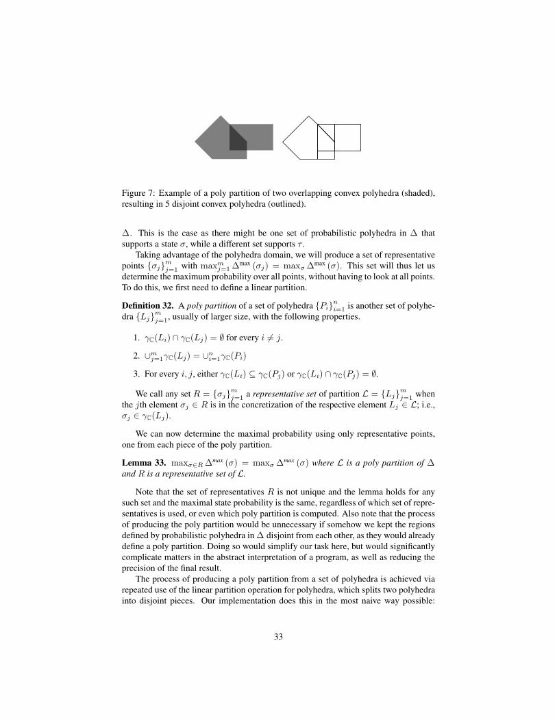
Figure 7: Example of a poly partition of two overlapping convex polyhedra (shaded),resulting in 5 disjoint convex polyhedra (outlined).
∆. This is the case as there might be one set of probabilistic polyhedra in ∆ thatsupports a state σ, while a different set supports τ .
Taking advantage of the polyhedra domain, we will produce a set of representativepoints {σj}mj=1 with maxmj=1 ∆max (σj) = maxσ ∆max (σ). This set will thus let usdetermine the maximum probability over all points, without having to look at all points.To do this, we first need to define a linear partition.
Definition 32. A poly partition of a set of polyhedra {Pi}ni=1 is another set of polyhe-dra {Lj}mj=1, usually of larger size, with the following properties.
1. γC(Li) ∩ γC(Lj) = ∅ for every i 6= j.
2. ∪mj=1γC(Lj) = ∪ni=1γC(Pi)
3. For every i, j, either γC(Li) ⊆ γC(Pj) or γC(Li) ∩ γC(Pj) = ∅.
We call any set R = {σj}mj=1 a representative set of partition L = {Lj}mj=1 whenthe jth element σj ∈ R is in the concretization of the respective element Lj ∈ L; i.e.,σj ∈ γC(Lj).
We can now determine the maximal probability using only representative points,one from each piece of the poly partition.
Lemma 33. maxσ∈R ∆max (σ) = maxσ ∆max (σ) where L is a poly partition of ∆and R is a representative set of L.
Note that the set of representatives R is not unique and the lemma holds for anysuch set and the maximal state probability is the same, regardless of which set of repre-sentatives is used, or even which poly partition is computed. Also note that the processof producing the poly partition would be unnecessary if somehow we kept the regionsdefined by probabilistic polyhedra in ∆ disjoint from each other, as they would alreadydefine a poly partition. Doing so would simplify our task here, but would significantlycomplicate matters in the abstract interpretation of a program, as well as reducing theprecision of the final result.
The process of producing a poly partition from a set of polyhedra is achieved viarepeated use of the linear partition operation for polyhedra, which splits two polyhedrainto disjoint pieces. Our implementation does this in the most naive way possible:
33
we maintain a bag of polyhedra, splitting any overlapping pairs, until no overlappingregions remain, as in the pseudo-code below.
poly-partition(Φ)def=
while ∃ C1, C2 ∈ Φ : ¬isempty(C1 uC C2)
Φ← (Φ− {C1, C2}) ∪ (C1 ↘↙ C2)
return Φ
We will write maxpp (∆) for maxσ ∆max (σ) to make explicit the method withwhich this value can be computed according to the lemma above.
Notation 34. If ∆ is a probabilistic polyhedron set over variables V , and σ is a stateover variables V ′ ⊆ V , then ∆ ∧ σ def
= ∆ ∧ B where B =∧x∈V ′ x = σ(x).
Definition 35. Given some probabilistic polyhedron set ∆1 and statement S where〈〈S〉〉∆1 terminates, let ∆2 = 〈〈S〉〉∆1 and ∆3 = ∆2 � L = {P ′i}. If for every σL ∈γP(C)({C ′i}) with ¬iszero(∆2∧σL) we have ∆4 = (∆2|σL) � H and maxpp (∆4) ≤t, then we write tsecuret(S,∆1).
Below we state the main soundness theorem for abstract interpretation using prob-abilistic polyhedron sets. This theorem states that the abstract interpretation just de-scribed can be used to soundly determine whether to accept a query.
Theorem 36. Let δ be an attacker’s initial belief. If δ ∈ γPn(P)(∆) and tsecuret(S,∆),then S is threshold secure for threshold t when evaluated with initial belief δ.
Note that the process described in computing threshold security involves merg-ing probabilistic polyhedra via the simplification operation (Definition 26); the orderin which these polyhedra are combined has no effect on soundness, but could affectprecision. We explore the variation possible in the precision due to ordering in Section7.3. The heuristic used for simplification in the abstract plus operation aims to optimizesome of these choices; further optimizations are part of our ongoing work.
7 ExperimentsWe have implemented an interpreter for the language in Figure 2 based on the prob-abilistic polyhedra powerset domain as well the simpler probabilistic domains con-structed from the interval and octagon base domains. The manipulations of base do-main regions are done using the Parma Polyhedra Library [6] (ppl-0.11.2). Countingcalculations are done using the LattE [21] tool (LattE macchiato 1.2-mk-0.9.3) in thecase of polyhedra and octagons. The trivial counting calculation for the interval do-main we implemented ourselves as part of the abstract interpreter, which itself is writ-ten in OCaml (3.12.0). While many of the abstract operations distribute over the setof probabilistic regions and thus could be parallelized, our implementation is currentlysingle-threaded.
This section presents an experimental evaluation of our implementation on severalbenchmark programs. Overall, the use of the octagonal and polyhedral domains re-sults in running times ranging from a few seconds to a few minutes. Compared to
34

enumeration-based approaches to probabilistic computation, using probabilistic poly-hedra improves running times by up to 1–2 orders of magnitude. Intervals do evenbetter, with running times ranging from tens to hundreds of milliseconds, constitutingan additional 1–2 orders of magnitude improvement. For our particular experiments,exact precision is reached by all domains if the bound on the number of regions issufficiently large.
Our experiments were conducted on a Mac Pro with two 2.26 GHz quad-core Xeonprocessors using 16 GB of RAM and running OS X v10.6.7.
7.1 Benchmark ProgramsWe applied our implementation to several queries. The timings measure, for eachquery, the construction of a pre-belief, the probabilistic evaluation of a query, and fi-nally a policy check over all secret variables. We describe each query here, and showthe complete source code, pre-belief, and further details in Appendix A.
Birthday We benchmark the birthday queries described in Section 2:
• bday 1 The first birthday query (Example 1).
• bday 1+2+special The sequence of the first two birthday queries (Example 1and then the same code, but with today increased by 1) followed by the specialbirthday query (Example 2). Below we refer to this benchmark as the birthdayquery sequence.
We consider small and large variants of these two queries: the former assumes the birthyear ranges from 1956 to 1992, while the latter uses the range 1910 to 2010.
Pizza This query evaluates whether a user might be interested in a local pizza parlor.To do this, the code checks whether the user’s location is within a certain square areaand whether they match an age or current education criteria most associated with pizza-eating habits (18-28 year old or currently undergrad or above). The modeled secretvariables thus include: the user’s birth year, the level of school currently being attended,and their address latitude and longitude (scaled by 106 and represented as an integer).The last two variables have large magnitudes. The true values used in the benchmarkwere 39003178 and 76958199 for latitude and longitude, respectively.
Photo This query is a direct encoding of a real targeted advertisement that Facebookincludes on their information page [4]. The query itself checks whether the user isfemale, engaged, and is in a certain age range, indicative of interest in (wedding) pho-tography service. There are three secret variables in this example: gender, relationshipstatus, and birth year.
Travel This query is another adaptation of a Facebook advertisement case study [3],based on a campaign run by a tourism agency. The aim of the query is to determinewhether the user lives in one of several relevant countries, speaks English, is over the
35

0
0.2
0.4
0.6
0.8
1
0 4 8 12 16
max
bel
ief
running time [s]
prob-scheme prob-poly-set
(a) birthday query bday 1 (small)
0
0.2
0.4
0.6
0.8
1
0 4 8 12 16 20 24 28 32 36
max
bel
ief
running time [s]
(b) birthday query, larger state space - bday 1 (large)
Figure 8: Query evaluation comparison
age of 21, and has completed a high level of education. The secret variables thusinclude four dimensions: the user’s country of residence, birth year, highest level ofcompleted education, and primary language.
Is Target Close, Who is Closer These queries were designed to demonstrate theneed for relational abstractions. They perform simple (Manhattan) distance calcula-tions over points defined by 2D coordinates. Is Target Close checks whether an un-known point is within some distance of a given point and Who is Closer determineswhich of two unknown points is closer to a given point. The nature of these queries isfurther discussed in Section 7.4 and their full specification is shown in Appendix B.
7.2 Comparison to EnumerationFigure 8(a) illustrates the result of running the bday 1 (small) query using our imple-mentation and one using Probabilistic Scheme [47], which is capable of sound prob-ability estimation after partial enumeration. Each × plots prob-scheme’s maximumprobability value (the y axis)—that is, the probability it assigns to the most likely se-cret state—when given a varying amount of time for sampling (the x axis). We can seethe precision improves steadily until it reaches the exact value of 1/259 at around 17seconds. Each + plots our implementation’s maximum probability value when given
36
an increasing number of probabilistic polyhedra; with a polyhedral bound of 2 (ormore), we obtain the exact value in less than one second. The timing measurementsare taken to be the medians of 20 runs.
The advantage of our approach is more evident in Figure 8(b) where we use thesame program but allow byear to span 1910 to 2010 rather than 1956 to 1992 (this isbday 1 (large)). In this case prob-scheme makes little progress even after a minute.Our approach, however, is unaffected by this larger state space and produces the exactmaximum belief in less than one second when using only 2 probabilistic polyhedra.
We can push the advantage much further with the use of the simpler interval do-main which can compute the exact probabilities in both the smaller and larger birthdayexamples, using only 2 intervals, in around 0.008 seconds. These benchmarks can beseen in Figure 9, discussed shortly.
7.3 Performance analysisFigures 9-13 summarize the performance results for all the benchmarks programs andfor each of the three base domains. The raw data producing these figures are found inTable 1 in the appendix. The bottom graph of each figure zooms in on the results forthe interval domain which can also be seen in the upper graphs.
The timing benchmarks in the figures are based on 20 runs, the median of which isdenoted by one of three symbols: a box, a diamond, and a pentagon for the interval,octagon, and polyhedron domains, respectively. The symbols are scaled based on theprecision in max probability, relative to exact, the analysis achieves; a tiny dot signi-fies exact probability and increasing symbol size signifies worsening precision. Note,however, that the sizes of the symbols are not proportional to precision. The verticalgray boxes range from the 1st to 3rd quartiles of the samples taken while the verticallines outside of these boxes represent the full extent of the samples.
We discuss the performance and precision aspects of these results in turn.
Performance. Overall, the use of the octagonal base domain results in slightly im-proved performance over the polyhedral base domain. The interval domain, however, ismuch faster than both due to the simpler counting and base domain operations. Thoughthe performance gains from the use of octagons are meager, we note that it is likely theycan be greatly improved by implementing a octagon-specialized counting method in-stead of using the general polyhedron counting tool (LattE).
As the number of base domain regions increases, the running time generally in-creases, though there are exceptions to this trend. A good example can be seen withintervals in Figure 10. Specifically, when there is no interval set size bound, the analy-sis takes a less time than with a bound of 40 (and even produces a more precise answer).In such situations the additional computational cost of manipulating a larger number ofregions is less than the cost that would have been incurred by having to merge them tomaintain some (large) bound.
In the cases of polyhedron and octagon base domains, the running time oddities aredue to the difficulty of accurately counting points in complex regions. We measuredthat, when evaluating the various queries in Figures 9-13, 95% or more of the running
37

0
2
4
6
8
10
1 2 3 4 5 6 7 8 910 15 20 25 30 35 40
time
[sec
onds
]
polygons octagons intervals
0.48 0.49
0.5 0.51 0.52 0.53 0.54
time
[sec
onds
]
set size bound
Figure 9: birthday query sequence benchmarks
time is spent in LattE, performing counting. Figure 14 plots the running time of LattEagainst the number of constraints used to define a polyhedron (we used the polyhedrathat arose when evaluating the above queries). Note that the y-axis is a log scale, andas such we can see the running time is super-exponential in the number of constraints.As such, overall running time is sensitive to the complexity of the polyhedra involved,even when they are few in number.
It turns out that when merging to respect the total bound can result in complicatedshapes which then, unintuitively, increase the running time. Two very stark examplesof this phenomenon are seen for in the pizza and travel queries (Figures 11 and 13respectively). With a region bound of one, the analysis of both these queries takesmuch longer than with the bound of two; the large amount of region merging in theseinstances resulted in a single, but highly complex region. Using octagons in both theseinstances does not result in complex regions which explains the massive performanceimprovement. These observations suggest a great deal of performance improvementcan be gained by simplifying the polyhedra if they become too complex.
Precision. The figures (and Table 1 in the appendix) generally show the trend that themaximum belief improves (decreases) as the region bound increases, though there are
38

0
5
10
15
1 2 3 4 5 6 7 8 910 15 20 25 30 35 40
time
[sec
onds
]
polygons octagons intervals
0.48
0.5
0.52
0.54
0.56
0.58
0.6
time
[sec
onds
]
set size bound
Figure 10: birthday (large) query sequence benchmarks
exceptions. A good example appears in Figure 9 which depicts the performance of thebirthday query sequence; with a set size bound of 3, the analysis is able to produce theexact max belief. Allowing 4 probabilistic polyhedra (or intervals, octagons), however,does not produce the exact belief anymore. The same occurs in Figure 10 for the largerstate space bday sequence benchmark.
The data also demonstrate that, as expected, the use of polyhedra is more precisethen use of octagons which itself is more precise than the use of intervals. For thebirthday queries, this difference manifests itself rarely, in particular for the set sizebound of 20 and 25 in Figure 9. In the pizza query benchmarks, polyhedra providea precision advantage over the other two domains when the region set size bound isbetween 5 and 10. Based on these sample queries, the precision advantage of usingpolyhedra or octagons over intervals seems insignificant. This is due to a general lack,in these queries, of conditionals that cannot be expressed exactly when using intervals(or octagons) exactly. Section 7.4 shows two queries that demonstrate the precisionadvantages of polyhedra and octagons more clearly.
Impact of merge order. Another reason for the the lack of a steady improvement ofprecision as the region bound increases is due to order in which polyhedra are merged.
39
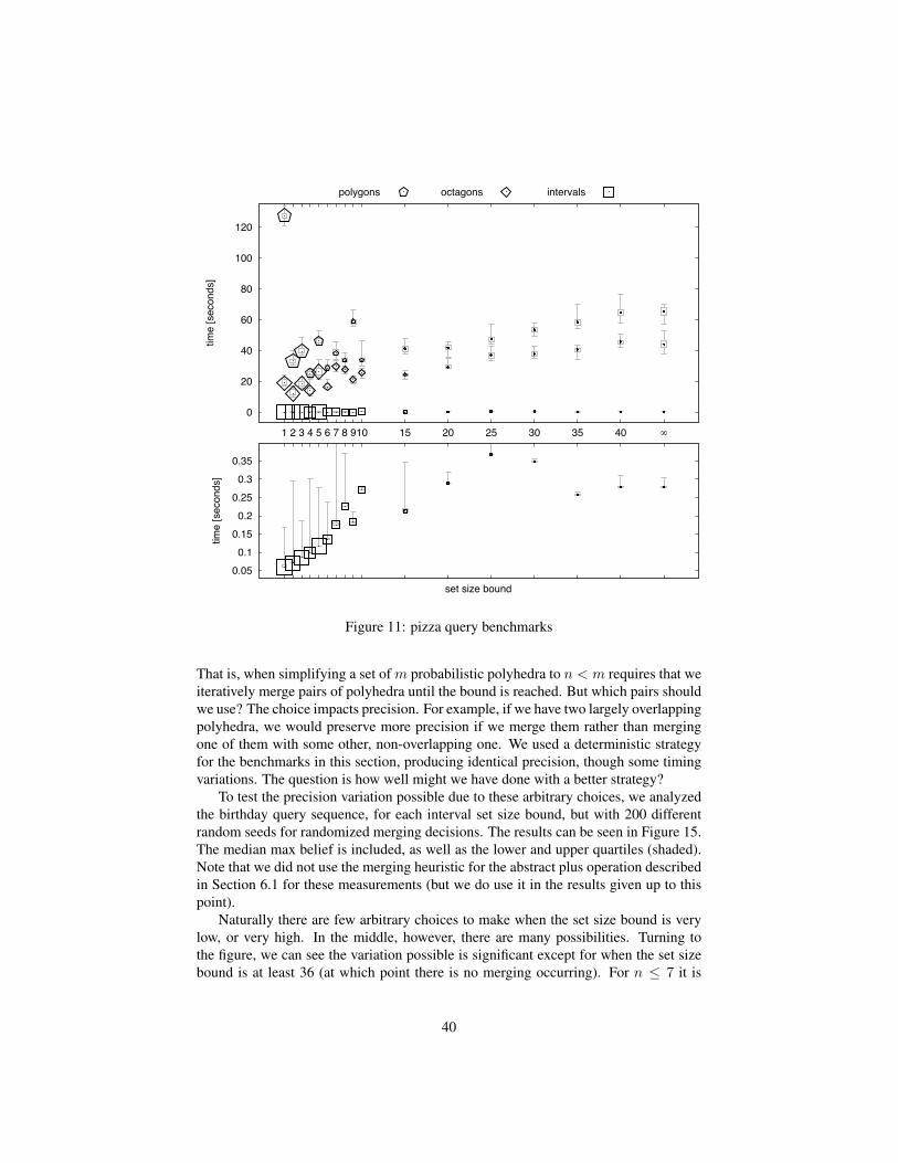
0
20
40
60
80
100
120
1 2 3 4 5 6 7 8 910 15 20 25 30 35 40
time
[sec
onds
]polygons octagons intervals
0.05 0.1
0.15 0.2
0.25 0.3
0.35
time
[sec
onds
]
set size bound
Figure 11: pizza query benchmarks
That is, when simplifying a set of m probabilistic polyhedra to n < m requires that weiteratively merge pairs of polyhedra until the bound is reached. But which pairs shouldwe use? The choice impacts precision. For example, if we have two largely overlappingpolyhedra, we would preserve more precision if we merge them rather than mergingone of them with some other, non-overlapping one. We used a deterministic strategyfor the benchmarks in this section, producing identical precision, though some timingvariations. The question is how well might we have done with a better strategy?
To test the precision variation possible due to these arbitrary choices, we analyzedthe birthday query sequence, for each interval set size bound, but with 200 differentrandom seeds for randomized merging decisions. The results can be seen in Figure 15.The median max belief is included, as well as the lower and upper quartiles (shaded).Note that we did not use the merging heuristic for the abstract plus operation describedin Section 6.1 for these measurements (but we do use it in the results given up to thispoint).
Naturally there are few arbitrary choices to make when the set size bound is verylow, or very high. In the middle, however, there are many possibilities. Turning tothe figure, we can see the variation possible is significant except for when the set sizebound is at least 36 (at which point there is no merging occurring). For n ≤ 7 it is
40

0
1
2
3
4
1 2 3 4 5 6 7 8 910 15 20 25 30 35 40
time
[sec
onds
]
polygons octagons intervals
0.014 0.016 0.018
0.02 0.022 0.024 0.026 0.028
0.03
time
[sec
onds
]
set size bound
Figure 12: photo query benchmarks
more likely than not to conclude max belief is 1, with 1 being the median. On the otherhand, from as little as n = 2, it is possible to do much better, even computing the exactbelief (lowest sample for n = 3). This itself suggests that our heuristic for the mergingorder in abstract plus is useful, as it managed to result in this exact max belief, againstall odds. Also, even though it did not produce exact beliefs for n > 3, it did a lot betterthan the trivial median one would get by performing merging randomly. Nevertheless,the merging order is an aspect of the implementation that has room for improvement,we consider some options in Section 8.
From n = 8, the random merging order starts producing non-trivial results, onaverage. Increasing n further makes it less and less likely to merge poorly; at n = 30for example, no random merge order out of the 200 samples managed to do terribly,all samples had belief below 0.01. Overall, the median max-belief is more or lessmonotonically improving as n increases as one would expect.
An interesting feature of Figure 15 is the best max-belief achieved for each n (thebottom mark of each column). This quantity seems to be getting worse from n = 3 allthe way to around n = 14 before it starts coming down again. We expect this is due totwo counteracting effects:
• Larger powerset size bound allows for more precise representation of distribu-
41

0
50
100
150
200
1 2 3 4 5 6 7 8 910 15 20 25 30 35 40
time
[sec
onds
]polygons octagons intervals
0.15 0.2
0.25 0.3
0.35 0.4
0.45 0.5
0.55 0.6
time
[sec
onds
]
set size bound
Figure 13: travel query benchmarks
0.01
0.1
1
10
100
0 10 20 30 40 50 60
time
[s]
num constraints
quartiles median
Figure 14: LattE benchmarks
42

2-3
2-2
2-1
20
1 2 3 4 5 6 7 8 9 10 11 12 13 14 15 16 17 18 19 20 21 22 23 24 25 26 27 28 29 30 31 32 33 34 35 36
max
bel
ief
interval set size bound n
median samples
Figure 15: birthday query sequence precision variation
tions, for some merging order.
• It is easier to find a good merging order if there are only a few options. For lowvalues of n, most merging orders are explored in the 200 samples, hence goodorders are found.
7.4 Relational queriesThe examples presented to this point are handled well by the interval-based abstraction,assuming a sufficient number of intervals are used. The simple interval-based abstrac-tion does not work so well programs that introduce relational constraints on variables.Such constraints can arise due to simple distance computations, which we would ex-pect to be found in many useful queries. We provide examples of such computationshere (the full specification of the queries appears in Appendix B).
Consider an initial belief composed of two pairs of 2-dimensional coordinates,specifying the location of two objects: (x1, y1), (x2, y2). The Is Target Close querychecks whether the first of the objects is within a specified distance d from a specifiedcoordinate (x, y). Distance is measured using Manhattan distance, that is |x − x1| +|y − y1| ≤ d.
Notice that if the first object is indeed within d of the target coordinate, we learn arelational constrains involving both x1 and y1, the coordinates of the first object:
x1 + y1 ≤ d+ x+ y ∧x1 − y1 ≤ d+ x− y ∧−x1 + y1 ≤ d− x+ y ∧−x1 − y1 ≤ d− x− y
Intervals are incapable of exact representation of relational constraints like x1 +y1 ≤ C. Octagons, however, are a suitable representation. Thus using our implemen-tation, the Is Target Close query fails (that is, overapproximates the probability of all
43
secret values to be 1) if interval base domain is used, regardless of the bound on numberof intervals used, but is exactly handled using only a few octagons.
The next query, Who Is Closer, determines which of the two given objects is closerto the target: |x − x1| + |y − y1| ≤ |x − x2| + |y − y2|. The truth of this equationimplies the disjunction of 4 constraints. One among them is the below.
x1 + y1 + x2 + y2 ≤ 2 ∗ x+ 2 ∗ y ∧x1 − y1 + x2 + y2 ≤ 2 ∗ x ∧−x1 + y1 + x2 + y2 ≤ 2 ∗ y ∧−x1 − y1 + x2 + y2 ≤ 0
While x and y can be treated as constants, such a constraint still involves four secretdimensions, x1, y1, x2, y2 and hence cannot be represented exactly using an octagon,which can express relational constraints of at most two dimensions. For this reason,our implementation fails when octagons are used (no matter their number), whereasthe polyhedra-based domain performs exact analysis with just a few polyhedra.
It is important to mention that our implementation does not split regions unlessperforming a conditioning operation. It might be beneficial in some cases to split aninterval into pieces so that their union is capable of better approximating relationalconstraints. We are considering such options for future work but several aspects of ourimplementation need to be improved to take advantage of this idea.
8 DiscussionThis section considers the some of the tradeoffs, challenges, design alternatives, andpossibilities for future work on knowledge-based security policies and probabilisticpolyhedra.
8.1 Knowledge-based policiesEmploying knowledge-based policies successfully requires maintaining a reasonableestimate of queriers’ beliefs. Two difficulties that arise in doing so are (1) establishingthe initial belief, and (2) accounting for collusion among queriers. Here we discussthese two issues, and suggest further applications of knowledge-based policies.
Initial belief. For P1 to enforce a knowledge-based policy on queries by P2 requiresthat P1 estimate P2’s belief about the possible valuations of P1’s secret data. WhenP2 has no particular knowledge of P1’s secrets, statistical demographic data can beused; e.g., the US Census and other public sources could be used for personal informa-tion. When P2 might have inside knowledge, P1 must expend more effort to accountfor it. For example, in a military setting, estimating a coalition partner’s estimate ofone’s resources could be derived from shared information, and from the likelihood ofP2 having acquired illicit information. Our benchmarks largely considered personal,private information, e.g., gender, age, level of education, etc. This information can be
44
drawn from public sources (e.g., Facebook demographics [1]). However, the distribu-tions we experimented with were oversimplifications of the actual, reported distribu-tions: they were largely simple, uniform distributions. At present, the syntax of ourquery language itself only allows specification of a single distribution. Of course, wecould permit users to more directly specify distributions of interest in a separate syntax.A more interesting alternative is to define the initial distribution using a probabilisticprogram employing conditioning based on observations, using the same mechanismsalready developed to determining whether to answer queries. This is done in languageslike IBAL [45] and Fun [11] and could be adapted to our setting.
If the initial belief estimate is (very) inaccurate, then P1 risks releasing informa-tion to P2 contrary to his intended policy. To “hedge his bets” against this possibility,he might choose to maintain a set of possible beliefs ∆, rather than a single beliefδ, and only release if the threshold was satisfied for every δ ∈ ∆. We return to thisidea in Section 9.3. In some sense we already do maintain multiple beliefs, as our im-plementation models/abstracts powersets of probabilistic polyhedra, rather than singlepolyhedra, for performance reasons. We leave to future work the exploration of thepractical implementation of this idea.
Collusion. Assuming that P maintains separate beliefs and thresholds for distinctqueriers Q1 and Q2, the possibility of collusion arises. Following our motivating ex-ample in the Introduction, P ’s privacy would be thwarted if he shared only his birth daywith Q1 and only his birth year with Q2 but then Q1 and Q2 shared their information.This problem is not unique to our work; the same problem would arise if P used anaccess control policy to protect birth day and birth year in the same way — the policywill be thwarted if Q1 and Q2 pool their information.
A simple approach to preventing this would be to model adversary knowledge glob-ally, effectively assuming that all queriers share their query results; doing so wouldprevent either Q1’s or Q2’s query (whichever was last). This approach is akin to hav-ing a global privacy budget in differential privacy (see Section 9.3) or a single, globalaccess control policy and would obviously harm utility. Moreover, because our querylanguage includes probabilistic if statements, using a global belief introduces an addi-tional, subtle complication: improbable results to non-deterministic queries (like Ex-ample 2) can make an adversary more uncertain of the secret value than before seeingthe query’s output. If it happens that the agents purported to be colluding are in factnot colluding then a global belief might under-approximate a non-colluding adversary’strue level of knowledge.
One possible compromise would be to consider both the potential of collusion andnon-collusion by tracking a global belief and a set of individual beliefs. When consid-ering a query, a rejection would be issued if either belief fails the policy check.
It is important to note that despite the possibility of a decrease certainty due toprobabilistic queries, rational adversaries, interested in maximizing their expectationof guessing the secret value, will take all query outputs into account; unlikely queryoutcomes are detrimental to certainty, but in expectation, potentially deceiving queriesincrease chances of guessing.
45
Further applications We have used the goal of decentralizing social networking ap-plications as a motivator for our technique. But knowledge-based policies have otherapplications as well. Here are four examples.
The first application is secure multiparty computation (SMC) [57]. Such computa-tions allow a set of mutually distrusting parties to compute a function f of their privateinputs while revealing nothing about their inputs beyond what is implied by the result.Depending on f , however, the result itself may reveal more information than partiesare comfortable with. Knowledge-based policies can generalized to this setting: eachparty X can assess whether the other parties Yi could have secret values such thatf ’s result would exceed a knowledge threshold about X’s secret. We have exploredtwo methods for implementing the generalized knowledge threshold check; details areelsewhere [34].
Another application is to protecting user browsing history. With the advent of “donot track” guidelines that forbid storing cookies to track users’ browsing habits acrosssites [23], service providers have turned to fingerprinting, which aims to identify auser based on available browser characteristics [10]. We can protect these attributeswith knowledge-based policies, and enforce them by analyzing the javascript codeon browsed pages. The flexibility of knowledge-based policies is useful: with ac-cess control we would have to choose, in advance, which attributes to reveal, but withknowledge-based policies we can set a threshold on the entire tuple of the most sensi-tive attributes and a web page can have access to whatever (legal) subset of informationit likes, for a better user experience.
A third application is to protect sensing capabilities. In particular, we can treatsensor readings as samples from a random process parameterized by confidential char-acteristics of the sensor. Each reading provides information about these parameters, inaddition to information from the reading itself. For example, suppose we want to sharemobility traces for traffic planning, but want to protect individuals’ privacy. We canview each trace as a series of samples from a random process that determines the indi-vidual’s location based on periodic factors, like previous location, time of day, day ofweek, etc. [51]. We can define the sampling function in our simple language, involvingprobabilistic choices over the hidden parameters. Belief tracking can be used to narrowdown the set of possible parameters to the model that could have produced the observedtraces; if the observer’s certainty about these parameters exceeds the threshold, then thetrace elements are not revealed. Note that trace obfuscation techniques are easily ac-counted for—they can simply be composed with the sampling function and reasonedabout together.
Finally, we observe that we can simply track the amount of released informationdue to an interaction as a degenerate case of enforcing knowledge-based policies. Inparticular, we can set the pre-belief over some sensitive information to be the uniformdistribution, and set the threshold to be 1. In this case, we will always answer anyquery, and at any time we can compute the entropy of the current belief estimate tocalculate the (maximum) number of bits leaked. This information may be used toevaluate the susceptibility to attack by gauging the confidence an attacker might havein their belief about secret information. It can be used to gauge what aspects of secretinformation were of interest to the attacker, giving hints to as their motive, or maybeeven differentiating an honest querier from a malicious one. Tracking information in
46
this manner is less expensive than enforcing threshold policies directly, since not allpossible outputs need to be considered, and carries no risk of a mis-estimate of thepre-belief: the number of reported leaked bits will be conservatively high.
8.2 Improving the Performance of Probabilistic PolyhedraWhile the performance of probabilistic polyhedra compares favorably to alternativeapproaches, it can nevertheless be improved; this will be important for applying it tothe deployment scenarios listed above. Here we present several ideas for improving theimplementation that we hope to explore in future work.
Handling nominal values. Our probabilistic domains are based on polyhedra, oc-tagons, and intervals, which are best for analyzing programs with numeric variables,that contain linear conditionals. Most of the variables in the benchmark programs wereof the numeric variety. However, some were nominal, e.g., the variable encoding auser’s language in the travel query, and these are unordered. Some variables are nomi-nal but partially ordered, like education level in the pizza query. While we can encodenominal values as integers, they may be better handled via other means, perhaps evenvia naıve enumeration. Handling of large quantities of nominal values could be per-formed symbolically using some of the tools used by other probabilistic languages:[12], graphical models [38], or factor graphs [11, 45]. Ideally abstract domains likeused in our system and ones better suited for nominal values, could be integrated (i.e.via reduced product [18]) to effectively process programs that contain both types ofvariables.
Region splitting. As the performance experiments in the previous section show, in-tervals can be far more efficient than polyhedra. While a single interval may be moreimprecise than a single polyhedron, an interesting idea is consider splitting a polyhe-dron into many intervals, aiming for the best of both worlds. The simplest means ofimplementing this idea is to modify the handling of the uniform statement for the pow-erset domains to result not in one, but several intervals. Though a single interval issufficient to exactly represent distributions produced by uniform, it would be insuffi-cient if, later, the program introduces relations not representable by intervals.
The challenge is to find the right tradeoff—increasing the number of intervals willslowly degrade performance and may hurt precision if we use an unfortunate mergingorder at join points, as seen in Figure 15. Heuristically picking the right merge order isa known challenge in abstract interpretation-based analyses.
Querier belief tracking. Recall a vital property of our knowledge-based policy en-forcement is simulatability: the adversary has (or is allowed to have) all the informationnecessary to decide the policy that governs its access, without interacting with the dataowner. As such, the computation of policy enforcement could, in theory, by done by thequerier. Naturally, they should not be trusted in this regard completely. One generaldirection is to imagine the querier performing the entire computation, and providingproof of the outcome, via something like proof-carrying code [43]. Alternatively, the
47

querier could provide hints to the data owner to improve the speed of his computation.For example, the querier could determine the optimal choices for merge order, and senda digest of these choices.
9 Related workWe consider four areas of work related to ours: systems aimed at protecting accessto users’ private data; methods for quantifying information flow from general-purposeprograms; methods for privacy-preserving computation, most notably differential pri-vacy; and finally approaches to performing general-purpose probabilistic computation.
9.1 Privacy enhancing network servicesSeveral recent proposals have considered alternative service architectures for better en-suring the privacy of individual participants. These systems tend to enforce access con-trol policies. For example, PrPl [50] is a decentralized social networking infrastructureaimed to permit participants to participate in social networking without losing owner-ship of their data. The system uses Personal-Cloud Butler services to store data andenforce access control policies. Persona [8] uses a centralized Facebook-style service,but users can store personal data on distributed storage servers that use attribute-basedencryption. Access to data is granted to those parties who have the necessary attributekeys. XBook [52] mediates social network data accesses by third-party application ex-tensions. Privad [28] is a privacy-preserving advertising platform that, like our runningexamples, runs the ad selection algorithm over the user’s data on the user’s platform.Privad presumes that outputs of ad selection reveal little about the inputs.
Knowledge-based security policies generalize access control policies: if we main-tain a belief estimate for each principal P , then the equivalent of granting P access todata d is to just set P ’s knowledge threshold for d to 1; for principalsR who should nothave access, the threshold for d is 0. Knowledge-based policies afford greater flexibilityby allowing partial access, i.e., when a threshold less than 1. Moreover, as mentionedin the introduction, we can set a policy on multiple data items, and thus grant moreaccess to one item than another (e.g., birth day and/or year) as long as knowledge ofthe aggregate is controlled.
9.2 Quantified information flowOthers have considered how an adversary’s knowledge of private data might be in-formed by a program’s output. Clark, Hunt, and Malacaria [13] define a static analysisthat bounds the secret information a straight-line program can leak in terms of equiv-alence relations between the inputs and outputs. Backes et al. [7] automate the syn-thesis of such equivalence relations and quantify leakage by computing the exact sizeof equivalence classes. Kopf and Rybalchenko [32] extend this approach, improvingits scalability by using sampling to identify equivalence classes and using under- andover-approximation to obtain bounds on their size. Mu and Clark [42] present a sim-
48
ilar analysis that uses over-approximation only. In all cases, the inferred equivalenceclasses can be used to compute entropy-based metrics of information leakage.
We differ from this work in two main ways. First, we implement a different securitycriterion. The most closely related metric is conditional vulnerability V as proposedby Smith [53], which can be defined using our notation as follows:
Definition 37. Let δ′ = [[S]]δ, where δ is the model of the querier’s initial belief.Then query S is vulnerability threshold secure iff for
V =∑
σL∈support(δ′�L)
(δ′ � L)(σL) · maxσH∈StateH
(δ′|σL � H)(σH)
we have V ≤ t for some threshold t.
The above definition is an expectation over all possible outputs σL, so unlikelyoutputs have less influence. Our notion of threshold security (Definition 3), in contrast,is equivalent to a bound on the following quantity:
V ∗ = maxσL∈support(δ′�L)
maxσH∈StateH
(δ′|σL � H)(σH)
This notion of security is strictly stronger as it considers each output individually:if any output, however unlikely, would increase knowledge beyond the threshold, thequery would be rejected. For example, recall the query from Example 1 where thesecret data bday is (assumed by the querier to be) uniformly distributed; call this queryS1. According to Definition 37, the minimum acceptable threshold for which the querywould be considered safe is V = 7
365 ∗17 + 358
365 ∗1
358 = 2/365 ≈ 0.005, whereasaccording to Definition 3, the minimum threshold is V ∗ = 1/7 ≈ 0.143.
The idea of strengthening of an entropy measure by eliminating the expectation hasbeen briefly considered by Kopf and Basin [31]. In their work this measure is proposedas a stronger alternative, a choice ultimately dependent on the application. In our case,however, the worst-case measure is absolutely necessary in order to prevent the leakageof information when rejecting a query.
The other distinguishing feature of our approach is that we keep an on-line modelof adversary knowledge according to prior, actual query results. Once a query is an-swered, the alternative possible outputs of this query no longer matter. To see thebenefit of this query-by-query approach, consider performing query S1 followed by aquery S2 which uses the same code as S1 (from Example 1) but has today = 265.With our system and bday = 270 the answer to S1 is False and with the revised beliefthe query S2 will be accepted as below threshold td = 0.2. If instead we had to modelthis pair of queries statically they would be rejected because (under the assumption ofuniformity) the pair of outputs True,True is possible and implies bday ∈ {265, 266}which would require td ≥ 0.5. Our approach also inherits from the belief-based ap-proach the ability to model a querier who is misinformed or incorrect, which can arisefollowing the result of a probabilistic query or because of a change to the secret databetween queries [14]. We note these advantages come at the cost of maintaining on-linebelief models.
Our proposed abstract domains are useful beyond the application of belief-basedthreshold security; e.g., they could be used to model uncertainty off-line (as in the
49
above work) rather than beliefs on-line, with the advantage that they are not limited touniform distributions (as required by [7, 32]).
McCamant and Ernst’s FLOWCHECK tool [37] measures the information releasedby a particular execution. However, it measures information release in terms of channelcapacity, rather than remaining uncertainty which is more appropriate for our setting.For example, FLOWCHECK would report a query that tries to guess a user’s birthdayleaks one bit regardless of whether the guess was successful, whereas the belief-basedmodel (and the other models mentioned above) would consider a failing guess to con-vey very little information (much less than a bit), and a successful guess conveyingquite a lot (much more than a bit).
9.3 Differential privacyA recent thread of research has aimed to enforce the privacy of database queries. Mostnotably, Dwork and colleagues have proposed differential privacy [24]: a differen-tially private query Q over a database of individuals’ records is a randomized functionthat produces roughly the same answer whether a particular individual’s data is in thedatabase or not. An appealing feature of this definition is that the querier’s knowledgeis not considered directly; rather, we are merely assured that Q’s answer will not dif-fer by much whether a particular individual is in the database or not. On the otherhand, differentially private databases require that individuals trust the database curator,a situation we would prefer to avoid, as motivated in the introduction.
We can compare differential privacy to our notion of threshold security by recastingthe differential privacy definition into the form of an adversarial privacy definition,which was formulated by Rastogi and Suciu to compare their own privacy definitionon databases to differential privacy [48]. Rastogi and Suciu’s definition is in termsof the presence or absence of a record in a database, whereas our notion is definedon secret states over variables in H . To bridge this gap suppose that, without lossof generality, variables x ∈ H range over {0, 1}, and we say a variable x is “in astate” σ when σ(x) = 1. (We can always encode an integer i as a sequence of bits.)Define δ({x1, ..., xn}) to be the probability of all states σ such that σ(xi) = 1 for all1 ≤ i ≤ n; i.e.,
δ({x1, ..., xn})def=
∑σ|σ(x1)=1∧...∧σ(xn)=1
δ(σ)
Then we can state adversarial privacy as follows.
Definition 38 (Adversarial Privacy). Given a query statement S , let O ⊆ StateL∪Hbe the set of all possible output states of S (over some set of secret variables H andpublic variables L), and ∆H ⊆ DistH be a set of distributions over secret states. Wesay that program S is ε-adversarially private w.r.t. ∆H iff for all adversary beliefsδH ∈ ∆H , all secret variables x ∈ H , and all possible outputs σo ∈ O, that δH({x}) ≤eε δ′H({x}). Here, δ′H = ([[S ]](δH × σL))|σo � H; that is, it is the revised adversarybelief after seeing that public output state of S is σo.
This definition says that query S is acceptable when the output of S increases onlyby a small multiplicative factor an adversary’s certainty that some variable x is in the
50
secret input state, for all adversaries whose prebeliefs are characterized by ∆H . Ras-togi and Suciu show that defining ∆H to be the class of planar, total sub-modular(or PTLM ) distributions renders an adversarial privacy definition equivalent to dif-ferential privacy. Among other conditions, PTLM distributions require fixed-sizeddatabases (which comes by construction in our setting), and require the probability ofone tuple’s presence to not be positively correlated with another’s. We can transfer thislatter condition to our setting by requiring that for all δ ∈ ∆H , and all x1, x2 ∈ H , wehave δ({x1})δ({x2}) ≤ δ({x1, x2}).
Comparing Definition 38 to Definition 3 we can see that the former makes a relativeassertion about the increased certainty of any one of a set of possible adversarial beliefs,while the latter makes an absolute assertion about the certainty of a single adversarialbelief. The absolute threshold of our definition is appealing, as is the more flexibleprebelief, which allows positive correlations among state variables. On the other hand,our definition assumes we have correctly modeled the adversary’s belief. While this ispossible in some cases, e.g., when demographic information is available, differentialprivacy is appealing in that it is robust a much larger number of adversaries, i.e., allthose whose prebeliefs are in PTLM .
Unfortunately, this strong privacy guarantee seems to come at strong cost to utility.For example, deterministic queries are effectively precluded, eliminating some possiblyuseful applications. For the application of social networks, Machanavajjhala et al. [33]have shown that good private social recommendations are feasible only for a small sub-set of the users in the social network or for a lenient setting of privacy parameters. Wecan see the utility loss in our motivating scenario as well. Consider the birthday queryfrom Example 1. Bob’s birthday being/not being in the query range influences the out-put of the query only by 1 (assuming yes/no is 1/0). One could add an appropriateamount of (Laplacian) noise to the query answer to hide what the true answer was andmake the query differentially private. However, this noise would be so large comparedto the original range {0, 1} that the query becomes essentially useless—the user wouldbe receiving a birthday announcement most days.4
By contrast, our approach permits answering (deterministic or randomized) queriesexactly if the release of information is below the threshold. Moreover, by trackingbeliefs between queries, there is no artificial limit on the number of queries since wecan track the released information exactly. Differential privacy imposes an artificiallimit on the number of queries because the post-query, revised beliefs of the adversaryare not computed. Rather, each query conservatively adds up to ε to an adversary’scertainty about a tuple, and since the precise release is not computed, we must assumethe worst. Eventually, performing further queries will pose too great of a risk.
As mentioned in the previous section, we could gain some of the privacy advantagesof differential privacy by modeling a (larger) set of beliefs rather than a single one.Our abstractions P and Pn (P) already model sets of distributions, rather than a singledistribution, so it remains interesting future work to exploit this representation towardincreasing privacy.
4By our calculations, with privacy parameter ε = 0.1 recommended by Dwork [24], the probability thequery returns the correct result is approximately 0.5249.
51

9.4 Probabilistic programmingThe core of our methodology relies on probabilistic computation. A variety of toolsexist for specifying random processes as computer programs and performing inferenceon them.
Implementations based on partial sampling [26, 44] or full enumeration [47] ofthe state space are unsuitable in our setting. Such tools are either too inefficient ortoo imprecise. Works based on smarter representations of probability distributions arepromising alternatives. Projects based on algebraic decision diagrams [12], graphicalmodels [38], and factor graphs [11, 45] translate programs into convenient structuresand take advantage of efficient algorithms for their manipulation or inference.
Our implementation for probabilistic computation and inference differs from exist-ing works in two main ways. Firstly, we are capable of approximation and hence cantrade off precision for performance, while maintaining soundness in terms of a strongsecurity policy. The second difference is the nature of our representation of probabilitydistributions. Our work is based on numerical abstractions: intervals, octagons, andpolyhedra. These abstractions are especially well suited for analysis of imperative pro-grams with numeric variables and linear conditionals. Other probabilistic languagesmight serve as better choices when nominal, rather than numeric, variables are used inqueries. The comparative study of the power and effectiveness of various representa-tions in probabilistic computation is a topic of our ongoing research.
We are not the first to propose probabilistic abstract interpretation. Monniaux [41]gives an abstract interpretation for probabilistic programs based on over-approximatingprobabilities of points. Di Pierro describes abstract interpretation for probabilisticlambda calculus [22]. Smith [54] describes probabilistic abstract interpretation forverification of quantitative program properties. Cousot [20] unifies these and otherprobabilistic program analysis tools. However, these do not deal with sound distribu-tion conditioning, the unique element of our approach, which is crucial for belief-basedinformation flow analysis.
10 ConclusionThis paper has explored the idea of knowledge-based security policies: given a queryover some secret data, that query should only be answered if doing so will not increasethe querier’s knowledge above a fixed threshold. We enforce knowledge-based poli-cies by explicitly tracking a model of a querier’s belief about secret data, representedas a probability distribution, and we deny any query that could increase knowledgeabove the threshold. Our denial criterion is independent of the actual secret, so denialdoes not leak information. We implement query analysis and belief tracking via ab-stract interpretation using domains of powersets of probabilistic polyhedra, octagons,and intervals. Compared to typical approaches to implementing belief revision, ourimplementation using this domain is more efficient and scales better.
Acknowledgments The authors are grateful to Jeff Foster, Nataliya Guts, the CSF’11 anony-mous referees, and especially Boris Kopf for their helpful comments on drafts of this paper.
52
This research was sponsored by the U.S. Army Research Laboratory and the U.K. Min-istry of Defence and was accomplished under Agreement Number W911NF-06-3-0001. Theviews and conclusions contained in this document are those of the author(s) and should not beinterpreted as representing the official policies, either expressed or implied, of the U.S. Army Re-search Laboratory, the U.S. Government, the U.K. Ministry of Defence or the U.K. Government.The U.S. and U.K. Governments are authorised to reproduce and distribute reprints for Govern-ment purposes notwithstanding any copyright notation hereon. Support was also provided byNational Science Foundation grants 0905419 and 0910530.
References[1] Facebook demographics and statistics report 2010. http://www.
istrategylabs.com/2010/01/facebook-demographics-and-
statistics- report-2010-145-growth-in-1-year, 2010.
[2] Statement of rights and responsibilities. http://www.facebook.com/terms.
php, October 2010.
[3] Facebook ads: A guide to targeting and reporting. http://www.
openforum.com/articles/facebook-ads-a-guide-to-targeting-
and-reporting-adele-cooper, 2011.
[4] Facebook ads: Case studies. http://www.facebook.com/advertising/
?campaign_id=402047449186, 2011.
[5] Facebook developers. http://developers.facebook.com, 2011. see thepolicy and docs/guides/canvas directories for privacy information.
[6] PPL: The Parma polyhedral library. http://www.cs.unipr.it/ppl/, 2011.
[7] Michael Backes, Boris Kopf, and Andrey Rybalchenko. Automatic discovery andquantification of information leaks. In Proceedings of the IEEE Symposium onSecurity and Privacy (S&P), 2009.
[8] Randy Baden, Adam Bender, Neil Spring, Bobby Bhattacharjee, and DanielStarin. Persona: an online social network with user-defined privacy. In Pro-ceedings of the ACM SIGCOMM Conference on Applications, Technologies, Ar-chitectures, and Protocols for Computer Communications (SIGCOMM), 2009.
[9] Roberto Bagnara, Patricia M. Hill, and Enea Zaffanella. Widening operators forpowerset domains. International Journal on Software Tools for Technology Trans-fer, 8(4):449–466, 2006.
[10] Karoly Boda, Adam Mate Foldes, Gabor Gyorgy Gulyas, and Sandor Imre. Usertracking on the web via cross-browser fingerprinting. In Proceedings of theNordic Conference in Secure IT Systems (NordSec), 2011.
53

[11] Johannes Borgstrom, Andrew D. Gordon, Michael Greenberg, James Margetson,and Jurgen Van Gael. Measure transformer semantics for bayesian machine learn-ing. In Proceedings of the European Symposium on Programming (ESOP), 2011.
[12] Guillaume Claret, Sriram K. Rajamani, Aditya V. Nori, Andrew D. Gordon, andJohannes Borgstroem. Bayesian inference for probabilistic programs via sym-bolic execution. Technical Report MSR-TR-2012-86, Microsoft Research, 2012.
[13] David Clark, Sebastian Hunt, and Pasquale Malacaria. Quantitative informa-tion flow, relations and polymorphic types. Journal of Logic and Computation,15:181–199, 2005.
[14] Michael R. Clarkson, Andrew C. Myers, and Fred B. Schneider. Quantifyinginformation flow with beliefs. Journal of Computer Security, 17(5):655–701,2009.
[15] Agostino Cortesi. Widening operators for abstract interpretation. In Proceedingsof the Sixth IEEE International Conference on Software Engineering and FormalMethods, pages 31–40, November 2008.
[16] Patrick Cousot and Radhia Cousot. Static determination of dynamic properties ofprograms. In Proceedings of the Second International Symposium on Program-ming, 1976.
[17] Patrick Cousot and Radhia Cousot. Abstract interpretation: a unified lattice modelfor static analysis of programs by construction or approximation of fixpoints. InProceedings of the ACM SIGPLAN Conference on Principles of ProgrammingLanguages (POPL), 1977.
[18] Patrick Cousot and Radhia Cousot. Systematic design of program analysis frame-works. In Proceedings of the Sixth International Symposium on Programming,1979.
[19] Patrick Cousot and Nicolas Halbwachs. Automatic discovery of linear restraintsamong variables of a program. In Proceedings of the ACM SIGPLAN Conferenceon Principles of Programming Languages (POPL), 1978.
[20] Patrick Cousot and Michael Monerau. Probabilistic abstract interpretation. InProceedings of the European Symposium on Programming (ESOP), 2012.
[21] Jesus A. De Loera, David Haws, Raymond Hemmecke, Peter Huggins, JeremyTauzer, and Ruriko Yoshida. Latte. http://www.math.ucdavis.edu/latte,2008.
[22] Alessandra Di Pierro, Chris Hankin, and Herbert Wiklicky. Probabilistic lambda-calculus and quantitative program analysis. Journal of Logic and Computation,15(2):159–179, 2005.
[23] Do not track. https://www.eff.org/issues/do-not-track, 2012.
54
[24] Cynthia Dwork. A firm foundation for private data analysis. Communications ofthe ACM, 54(1):86–95, 2011.
[25] Philippe Golle. Revisiting the uniqueness of simple demographics in the us pop-ulation. In Proceedings of the Workshop on Privacy in the Electronic Society(WPES), 2006.
[26] Noah D. Goodman, Vikash K. Mansinghka, Daniel M. Roy, Keith Bonawitz, andJoshua B. Tenenbaum. Church: a language for generative models. In Proceedingsof the Conference on Uncertainty in Artificial Intelligence (UAI), 2008.
[27] Saikat Guha, Bin Cheng, and Paul Francis. Challenges in measuring online adver-tising systems. In Proceedings of the Internet Measurement Conference (IMC),2010.
[28] Saikat Guha, Bin Cheng, and Paul Francis. Privad: Practical privacy in onlineadvertising. In Proceedings of the Symposium on Networked Systems Design andImplementation (NSDI), March 2011.
[29] Krishnaram Kenthapadi, Nina Mishra, and Kobbi Nissim. Simulatable auditing.In Proceedings of the ACM SIGMOD Symposium on Principles of Database Sys-tems (PODS), 2005.
[30] Oleg Kiselyov and Chung-Chieh Shan. Embedded probabilistic programming. InProceedings of the Working Conference on Domain Specific Languages (DSL),2009.
[31] Boris Kopf and David Basin. An Information-Theoretic Model for Adaptive Side-Channel Attacks. In Proceedings of the ACM Conference on Computer and Com-munications Security (CCS), 2007.
[32] Boris Kopf and Andrey Rybalchenko. Approximation and randomization forquantitative information-flow analysis. In Proceedings of the IEEE ComputerSecurity Foundations Symposium (CSF), 2010.
[33] Ashwin Machanavajjhala, Aleksandra Korolova, and Atish Das Sarma. Personal-ized social recommendations: accurate or private. In Proceedings of the Interna-tional Conference on Very Large Data Bases (VLDB), 2011.
[34] Piotr Mardziel, Michael Hicks, Jonathan Katz, and Mudhakar Srivatsa.Knowledge-oriented secure multiparty computation. In Proceedings of the ACMSIGPLAN Workshop on Programming Languages and Analysis for Security(PLAS), 2012.
[35] Piotr Mardziel, Stephen Magill, Michael Hicks, and Mudhakar Srivatsa. Dynamicenforcement of knowledge-based security policies. In Proceedings of the IEEEComputer Security Foundations Symposium (CSF), 2011.
[36] Piotr Mardziel, Stephen Magill, Michael Hicks, and Mudhakar Srivatsa. Dynamicenforcement of knowledge-based security policies. Technical Report CS-TR-4978, University of Maryland Department of Computer Science, 2011.
55

[37] Stephen McCamant and Michael D. Ernst. Quantitative information flow as net-work flow capacity. In Proceedings of the ACM SIGPLAN Conference on Pro-gramming Language Design and Implementation (PLDI), 2008.
[38] Brian Milch, Bhaskara Marthi, Stuart Russell, David Sontag, Daniel L. Ong, andAndrey Kolobov. Blog: Probabilistic models with unknown objects. In Pro-ceedings of the International Joint Conference on Artificial Intelligence (IJCAI),2005.
[39] Antoine Mine. The octagon abstract domain. In Proceedings of the WorkingConference on Reverse Engineering (WCRE), 2001.
[40] David Monniaux. Abstract interpretation of probabilistic semantics. In Proceed-ings of the Static Analysis Symposium (SAS), 2000.
[41] David Monniaux. Analyse de programmes probabilistes par interpretation ab-straite. These de doctorat, Universite Paris IX Dauphine, 2001.
[42] Chunyan Mu and David Clark. An interval-based abstraction for quantifyinginformation flow. Electronic Notes in Theoretical Computer Science, 253(3):119–141, 2009.
[43] George C. Necula. Proof-carrying code. In Proceedings of the ACM SIGPLANConference on Principles of Programming Languages (POPL), pages 106–119,1997.
[44] Sungwoo Park, Frank Pfenning, and Sebastian Thrun. A probabilistic languagebased on sampling functions. ACM Transactions on Programming Languagesand Systems (TOPLAS), 31(1):4:1–4:46, 2008.
[45] Avi Pfeffer. The design and implementation of IBAL: A general-purpose proba-bilistic language. In Lise Getoor and Benjamin Taskar, editors, Statistical Rela-tional Learning. MIT Press, 2007.
[46] Corneliu Popeea and Wei-ngan Chin. Inferring disjunctive postconditions. InProceedings of the Asian Computing Science Conference (ASIAN), 2006.
[47] Alexey Radul. Report on the probabilistic language Scheme. In Proceedings ofthe Dynamic Languages Symposium (DLS), 2007.
[48] Vibhor Rastogi, Michael Hay, Gerome Miklau, and Dan Suciu. Relationship pri-vacy: output perturbation for queries with joins. In Proceedings of the Symposiumon Principles of Database Systems (PODS), 2009.
[49] Alfredo Rial and George Danezis. Privacy-preserving smart metering. In Pro-ceedings of the Workshop on Privacy in the Electronic Society (WPES), 2011.
[50] Seok-Won Seong, Jiwon Seo, Matthew Nasielski, Debangsu Sengupta, Sudheen-dra Hangal, Seng Keat Teh, Ruven Chu, Ben Dodson, and Monica S. Lam. PrPl:a decentralized social networking infrastructure. In Proceedings of the Workshopon Mobile Cloud Computing & Services: Social Networks and Beyond, 2010.Invited Paper.
56
[51] Reza Shokri, George Theodorakopoulos, Jean-Yves Le Boudec, and Jean-PierreHubaux. Quantifying Location Privacy. In Proceedings of the IEEE Symposiumon Security and Privacy (S&P), pages 247–262, 2011.
[52] Kapil Singh, Sumeer Bhola, and Wenke Lee. xBook: Redesigning privacy controlin social networking platforms. In Proceedings of the USENIX Security Sympo-sium, 2009.
[53] Geoffrey Smith. On the foundations of quantitative information flow. In Pro-ceedings of the Conference on Foundations of Software Science and ComputationStructures (FoSSaCS), 2009.
[54] Michael J. A. Smith. Probabilistic abstract interpretation of imperative programsusing truncated normal distributions. Electronic Notes in Theoretical ComputerScience, 220(3):43–59, 2008.
[55] Latanya Sweeney. Simple demographics often identify people uniquely. Techni-cal Report LIDAP-WP4, Carnegie Mellon University, School of Computer Sci-ence, Data Privacy Laboratory, 2000.
[56] David Worthington. Mypace user data for sale. PC World on-line, March2010. http://www.pcworld.com/article/191716/myspace_user_data_
for_sale.html.
[57] Andrew Chi-Chih Yao. How to generate and exchange secrets. In Proceedingsof the Annual Symposium on Foundations of Computer Science, pages 162–167,1986.
A Example queriesWe provide here the queries and prebeliefs we used for the experiments in Section 7.The queries are described as functions from some set of inputs to some set of outputs.The exact syntax is as follows.
querydef queryname in1 · · · inn → out1 · · · outm :querybody
Query definitions that follow sometimes include pre-processing statements of theform:
#define x = exp
Such statements result in any occurrence of a variable x being replaced by the expres-sion exp. This is used for convenience to refer to common expressions without actuallyrequiring the analysis to track additional variables/dimensions.
57
To specify a query invocation we use the following syntax.
query queryname :in1 := val1;· · ·inn := valn
Each experiment must also specify the values of the secrets being queried, and thequerier’s prebelief. Each specification is a merely a program that sets the values of thesevariables. For the actual secret values this program begins with the declaration secret;the resulting state of executing program is taken to be the secret state. The programto set the prebelief begins belief and has the same format; note that this program willuse pif or uniform x n1 n2 to give secrets different possible values with differentprobabilities.
We now give the content of the queries used in the experiments.
A.1 BirthdayFor the small stateset size birthday experiments we used the following secret and pre-belief.
secret :
s bday := 270 ;s byear := 1980
belief :
uniform s bday 0 364 ;uniform s byear 1956 1992
The two queries used were as follows.
querydef bday : c day → out
if s bday ≥ c day ∧ c day + 7 > s bday thenout := 1
elseout := 0
querydef spec : c year → out
#define age = c year − s byearif age = 10 ∨ age = 20 ∨ age = 30 ∨ age = 40∨ age = 50 ∨ age = 60 ∨ age = 70 ∨ age = 80∨ age = 90 ∨ age = 100 thenout := 1
elseout := 0 ;
pif 1/10 thenout := 1
The statistics described in comparison to the enumeration approach (Section 7.2)include the time spent processing this initial setup as well as time processing one birth-day query. Figure 10 benchmarks two bday queries followed by a spec year query.
58
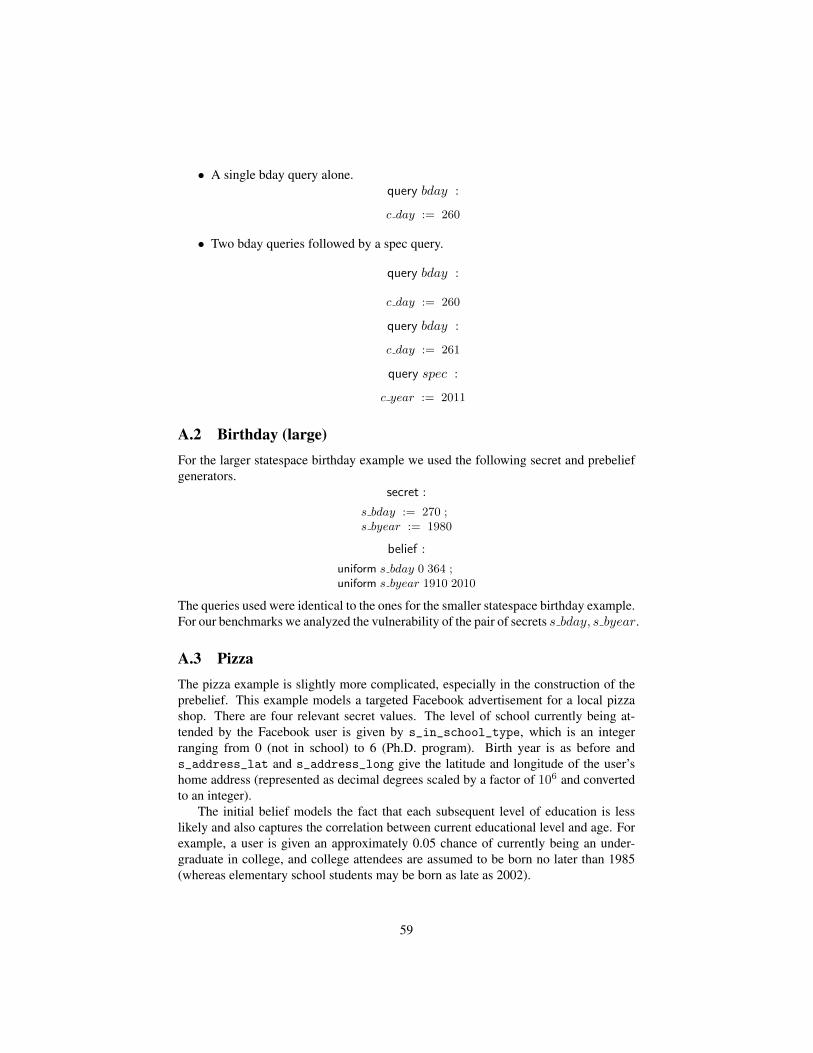
• A single bday query alone.query bday :
c day := 260
• Two bday queries followed by a spec query.
query bday :
c day := 260
query bday :
c day := 261
query spec :
c year := 2011
A.2 Birthday (large)For the larger statespace birthday example we used the following secret and prebeliefgenerators.
secret :
s bday := 270 ;s byear := 1980
belief :
uniform s bday 0 364 ;uniform s byear 1910 2010
The queries used were identical to the ones for the smaller statespace birthday example.For our benchmarks we analyzed the vulnerability of the pair of secrets s bday, s byear.
A.3 PizzaThe pizza example is slightly more complicated, especially in the construction of theprebelief. This example models a targeted Facebook advertisement for a local pizzashop. There are four relevant secret values. The level of school currently being at-tended by the Facebook user is given by s_in_school_type, which is an integerranging from 0 (not in school) to 6 (Ph.D. program). Birth year is as before ands_address_lat and s_address_long give the latitude and longitude of the user’shome address (represented as decimal degrees scaled by a factor of 106 and convertedto an integer).
The initial belief models the fact that each subsequent level of education is lesslikely and also captures the correlation between current educational level and age. Forexample, a user is given an approximately 0.05 chance of currently being an under-graduate in college, and college attendees are assumed to be born no later than 1985(whereas elementary school students may be born as late as 2002).
59
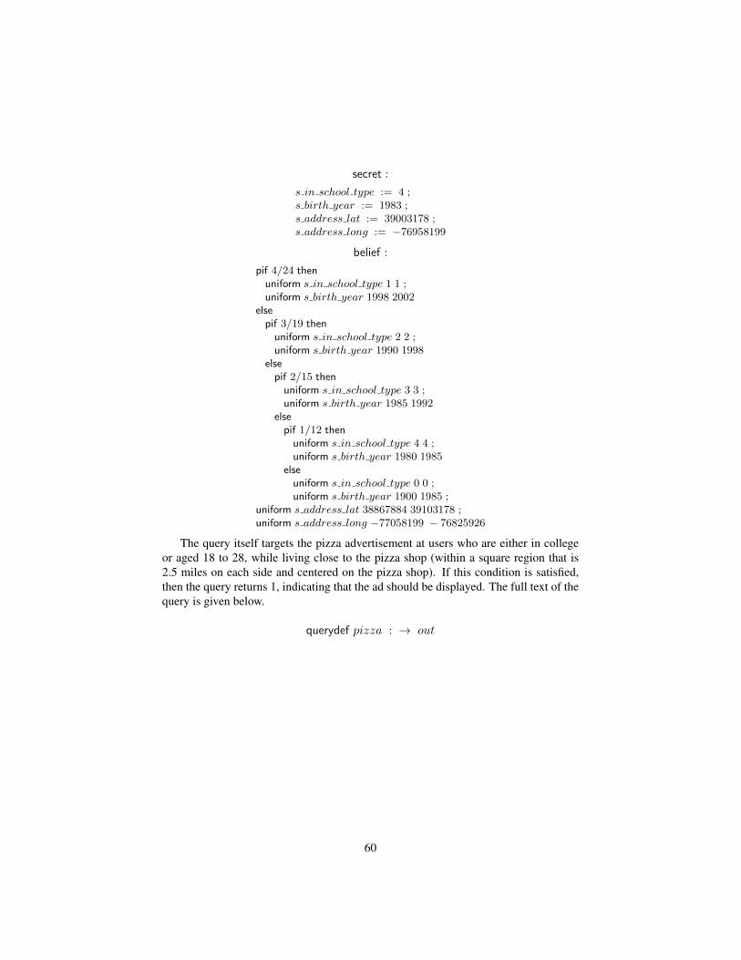
secret :
s in school type := 4 ;s birth year := 1983 ;s address lat := 39003178 ;s address long := −76958199
belief :
pif 4/24 thenuniform s in school type 1 1 ;uniform s birth year 1998 2002
elsepif 3/19 then
uniform s in school type 2 2 ;uniform s birth year 1990 1998
elsepif 2/15 then
uniform s in school type 3 3 ;uniform s birth year 1985 1992
elsepif 1/12 then
uniform s in school type 4 4 ;uniform s birth year 1980 1985
elseuniform s in school type 0 0 ;uniform s birth year 1900 1985 ;
uniform s address lat 38867884 39103178 ;uniform s address long −77058199 − 76825926
The query itself targets the pizza advertisement at users who are either in collegeor aged 18 to 28, while living close to the pizza shop (within a square region that is2.5 miles on each side and centered on the pizza shop). If this condition is satisfied,then the query returns 1, indicating that the ad should be displayed. The full text of thequery is given below.
querydef pizza : → out
60
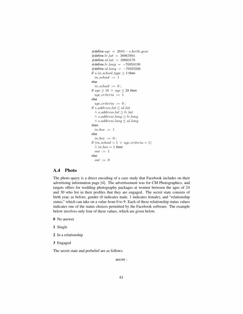
#define age = 2010− s birth year#define lr lat = 38967884#define ul lat = 39003178#define lr long = −76958199#define ul long = −76925926if s in school type ≥ 4 thenin school := 1
elsein school := 0 ;
if age ≥ 18 ∧ age ≤ 28 thenage criteria := 1
elseage criteria := 0 ;
if s address lat ≤ ul lat∧ s address lat ≥ lr lat∧ s address long ≥ lr long∧ s address long ≤ ul long
thenin box := 1
elsein box := 0 ;
if (in school = 1 ∨ age criteria = 1)∧ in box = 1 thenout := 1
elseout := 0
A.4 PhotoThe photo query is a direct encoding of a case study that Facebook includes on theiradvertising information page [4]. The advertisement was for CM Photographics, andtargets offers for wedding photography packages at women between the ages of 24and 30 who list in their profiles that they are engaged. The secret state consists ofbirth year, as before, gender (0 indicates male, 1 indicates female), and “relationshipstatus,” which can take on a value from 0 to 9. Each of these relationship status valuesindicates one of the status choices permitted by the Facebook software. The examplebelow involves only four of these values, which are given below.
0 No answer
1 Single
2 In a relationship
3 Engaged
The secret state and prebelief are as follows.
secret :
61

s birth year := 1983 ;s gender := 0 ;s relationship status := 0
belief :
uniform s birth year 1900 2010 ;uniform s gender 0 1 ;uniform s relationship status 0 3
The query itself is the following.
querydef cm advert : → out
#define age = 2010− s birth yearif age ≥ 24 ∧ age ≤ 30 thenage sat := 1
elseage sat := 0 ;
if s gender = 1∧ s relationship status = 3∧ age sat = 1 thenout := 1
elseout := 0
A.5 TravelThis example is another Facebook advertising case study [3]. It is based on an ad cam-paign run by Britain’s national tourism agency, VisitBritain. The campaign targetedEnglish-speaking Facebook users currently residing in countries with strong ties to theUnited Kingdom. They further filtered by showing the advertisement only to collegegraduates who were at least 21 years of age.
We modeled this using four secret values: country, birth year, highest completededucation level, and primary language. As with other categorical data, we representlanguage and country using an enumeration. We ranked countries by number of Face-book users as reported by socialbakers.com. This resulted in the US being countrynumber 1 and the UK being country 3. To populate the list of countries with “strongconnections” to the UK, we took a list of former British colonies. For the languageattribute, we consider a 50-element enumeration where 0 indicates “no answer” and 1indicates “English” (other values appear in the prebelief but are not used in the query).
secret :
country := 1 ;birth year := 1983 ;completed school type := 4 ;language := 5
belief :
62
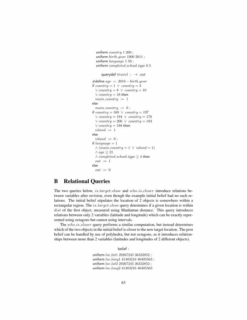
uniform country 1 200 ;uniform birth year 1900 2011 ;uniform language 1 50 ;uniform completed school type 0 5
querydef travel : → out
#define age = 2010− birth yearif country = 1 ∨ country = 3∨ country = 8 ∨ country = 10∨ country = 18 thenmain country := 1
elsemain country := 0 ;
if country = 169 ∨ country = 197∨ country = 194 ∨ country = 170∨ country = 206 ∨ country = 183∨ country = 188 thenisland := 1
elseisland := 0 ;
if language = 1∧ (main country = 1 ∨ island = 1)∧ age ≥ 21∧ completed school type ≥ 4 thenout := 1
elseout := 0
B Relational QueriesThe two queries below, is target close and who is closer introduce relations be-tween variables after revision, even though the example initial belief had no such re-lations. The initial belief stipulates the location of 2 objects is somewhere within arectangular region. The is target close query determines if a given location is withindist of the first object, measured using Manhattan distance. This query introducesrelations between only 2 variables (latitude and longitude) which can be exactly repre-sented using octagons but cannot using intervals.
The who is closer query performs a similar computation, but instead determineswhich of the two objects in the initial belief is closer to the new target location. The postbelief can be handled by use of polyhedra, but not octagons, as it introduces relation-ships between more than 2 variables (latitudes and longitudes of 2 different objects).
belief :
uniform loc lat1 29267245 36332852 ;uniform loc long1 41483216 46405563 ;uniform loc lat2 29267245 36332852 ;uniform loc long2 41483216 46405563
63

querydef is target close : target location lat target location long dist → is close
is close := 0 ;dist lat := loc lat1− target location lat ;dist long := loc long1− target location long ;if dist lat < 0 thendist lat := −1× dist lat ;
if dist long < 0 thendist long := −1× dist long ;
if dist lat+ dist long ≤ dist thenis close := 1
querydef who is closer : target location lat target location long → who closer
diff lat1 := loc lat1− target location lat ;diff long1 := loc long1− target location long ;diff lat2 := loc lat2− target location lat ;diff long2 := loc long2− target location long ;if diff lat1 < 0 thendiff lat1 := −1× diff lat1 ;
if diff long1 < 0 thendiff long1 := −1× diff long1 ;
if diff lat2 < 0 thendiff lat2 := −1× diff lat2 ;
if diff long2 < 0 thendiff long2 := −1× diff long2 ;
dist1 := diff long1 + diff lat1 ;dist2 := diff long2 + diff lat2 ;if dist1 ≤ dist2 thenwho closer := 0
elsewho closer := 1
C Benchmark ResultsTable 1 tabulates performance results for all of the benchmark programs, for each possi-ble base domain (intervals, octagons, and polyhedra labeled 2, 3, and D respectively).Each column is the maximum size of the permitted powerset, whereas each groupingof rows contains, respectively, the wall clock time in seconds (median of 20 runs), therunning time’s semi-interquartile range (SIQR) with the number of outliers in paren-theses (which are defined to be the points 3 × SIQR below the first quartile or abovethe third), and the max belief computed (smaller being more accurate).
64
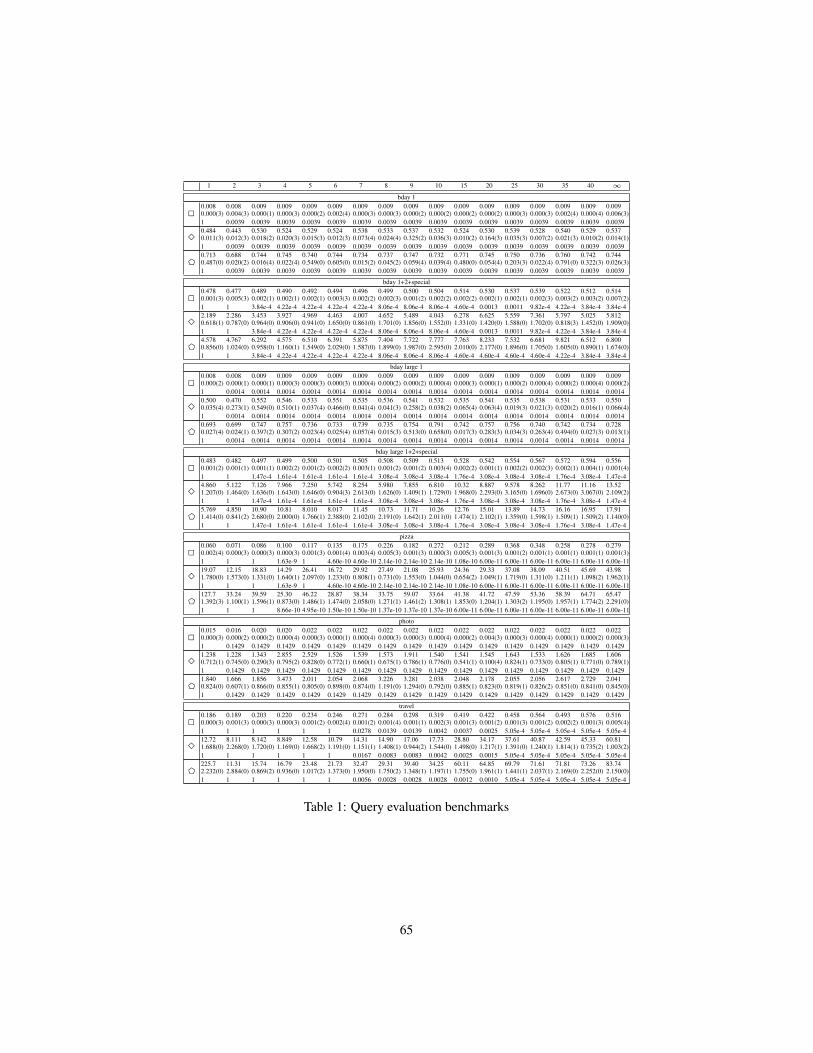
1 2 3 4 5 6 7 8 9 10 15 20 25 30 35 40 ∞
bday 1
20.0080.000(3)1
0.0080.004(3)0.0039
0.0090.000(1)0.0039
0.0090.000(3)0.0039
0.0090.000(2)0.0039
0.0090.002(4)0.0039
0.0090.000(3)0.0039
0.0090.000(3)0.0039
0.0090.000(2)0.0039
0.0090.000(2)0.0039
0.0090.000(2)0.0039
0.0090.000(2)0.0039
0.0090.000(3)0.0039
0.0090.000(3)0.0039
0.0090.002(4)0.0039
0.0090.000(4)0.0039
0.0090.006(3)0.0039
30.4840.011(3)1
0.4430.012(3)0.0039
0.5300.018(2)0.0039
0.5240.020(3)0.0039
0.5290.015(3)0.0039
0.5240.012(3)0.0039
0.5380.073(4)0.0039
0.5330.024(4)0.0039
0.5370.325(2)0.0039
0.5320.036(3)0.0039
0.5240.010(2)0.0039
0.5300.164(3)0.0039
0.5390.035(3)0.0039
0.5280.007(2)0.0039
0.5400.021(3)0.0039
0.5290.010(2)0.0039
0.5370.014(1)0.0039
D0.7130.487(0)1
0.6880.020(2)0.0039
0.7440.016(4)0.0039
0.7450.022(4)0.0039
0.7400.549(0)0.0039
0.7440.605(0)0.0039
0.7340.015(2)0.0039
0.7370.045(2)0.0039
0.7470.059(4)0.0039
0.7320.039(4)0.0039
0.7710.480(0)0.0039
0.7450.054(4)0.0039
0.7500.203(3)0.0039
0.7360.022(4)0.0039
0.7600.791(0)0.0039
0.7420.322(3)0.0039
0.7440.026(3)0.0039
bday 1+2+special
20.4780.001(3)1
0.4770.005(3)1
0.4890.002(1)3.84e-4
0.4900.002(1)4.22e-4
0.4920.002(1)4.22e-4
0.4940.003(3)4.22e-4
0.4960.002(2)4.22e-4
0.4990.002(3)8.06e-4
0.5000.001(2)8.06e-4
0.5040.002(2)8.06e-4
0.5140.002(2)4.60e-4
0.5300.002(1)0.0013
0.5370.002(1)0.0011
0.5390.002(3)9.82e-4
0.5220.003(2)4.22e-4
0.5120.003(2)3.84e-4
0.5140.007(2)3.84e-4
32.1890.618(1)1
2.2860.787(0)1
3.4530.964(0)3.84e-4
3.9270.906(0)4.22e-4
4.9690.941(0)4.22e-4
4.4631.650(0)4.22e-4
4.0070.861(0)4.22e-4
4.6521.701(0)8.06e-4
5.4891.856(0)8.06e-4
4.0431.552(0)8.06e-4
6.2781.331(0)4.60e-4
6.6251.420(0)0.0013
5.5591.588(0)0.0011
7.3611.702(0)9.82e-4
5.7970.818(3)4.22e-4
5.0251.452(0)3.84e-4
5.8121.909(0)3.84e-4
D4.5780.856(0)1
4.7671.024(0)1
6.2920.958(0)3.84e-4
4.5751.160(1)4.22e-4
6.5101.549(0)4.22e-4
6.3912.029(0)4.22e-4
5.8751.587(0)4.22e-4
7.4041.899(0)8.06e-4
7.7221.987(0)8.06e-4
7.7772.595(0)8.06e-4
7.7632.010(0)4.60e-4
8.2332.177(0)4.60e-4
7.5321.896(0)4.60e-4
6.6811.705(0)4.60e-4
9.8211.605(0)4.22e-4
6.5120.890(1)3.84e-4
6.8001.674(0)3.84e-4
bday large 1
20.0080.000(2)1
0.0080.000(1)0.0014
0.0090.000(1)0.0014
0.0090.000(3)0.0014
0.0090.000(3)0.0014
0.0090.000(3)0.0014
0.0090.000(4)0.0014
0.0090.000(2)0.0014
0.0090.000(2)0.0014
0.0090.000(4)0.0014
0.0090.000(3)0.0014
0.0090.000(1)0.0014
0.0090.000(2)0.0014
0.0090.000(4)0.0014
0.0090.000(2)0.0014
0.0090.000(4)0.0014
0.0090.000(2)0.0014
30.5000.035(4)1
0.4700.273(1)0.0014
0.5520.549(0)0.0014
0.5460.510(1)0.0014
0.5330.037(4)0.0014
0.5510.466(0)0.0014
0.5350.041(4)0.0014
0.5360.041(3)0.0014
0.5410.258(2)0.0014
0.5320.038(2)0.0014
0.5350.065(4)0.0014
0.5410.063(4)0.0014
0.5350.019(3)0.0014
0.5380.021(3)0.0014
0.5310.020(2)0.0014
0.5330.016(1)0.0014
0.5500.066(4)0.0014
D0.6930.027(4)1
0.6990.024(1)0.0014
0.7470.397(2)0.0014
0.7570.307(2)0.0014
0.7360.023(4)0.0014
0.7330.025(4)0.0014
0.7390.057(4)0.0014
0.7350.015(3)0.0014
0.7540.513(0)0.0014
0.7910.658(0)0.0014
0.7420.017(3)0.0014
0.7570.283(3)0.0014
0.7560.034(3)0.0014
0.7400.263(4)0.0014
0.7420.494(0)0.0014
0.7340.027(3)0.0014
0.7280.013(1)0.0014
bday large 1+2+special
20.4830.001(2)1
0.4820.001(1)1
0.4970.001(1)1.47e-4
0.4990.002(2)1.61e-4
0.5000.001(2)1.61e-4
0.5010.002(2)1.61e-4
0.5050.003(1)1.61e-4
0.5080.001(2)3.08e-4
0.5090.001(2)3.08e-4
0.5130.003(4)3.08e-4
0.5280.002(2)1.76e-4
0.5420.001(1)3.08e-4
0.5540.002(2)3.08e-4
0.5670.002(3)3.08e-4
0.5720.002(1)1.76e-4
0.5940.004(1)3.08e-4
0.5560.001(4)1.47e-4
34.8601.207(0)1
5.1221.464(0)1
7.1261.636(0)1.47e-4
7.9661.643(0)1.61e-4
7.2501.646(0)1.61e-4
5.7420.904(3)1.61e-4
8.2542.613(0)1.61e-4
5.9801.626(0)3.08e-4
7.8551.409(1)3.08e-4
6.8101.729(0)3.08e-4
10.321.968(0)1.76e-4
8.8872.293(0)3.08e-4
9.5783.165(0)3.08e-4
8.2621.696(0)3.08e-4
11.772.673(0)1.76e-4
11.163.067(0)3.08e-4
13.522.109(2)1.47e-4
D5.7691.414(0)1
4.8500.841(2)1
10.902.680(0)1.47e-4
10.812.000(0)1.61e-4
8.0101.766(1)1.61e-4
8.0172.388(0)1.61e-4
11.452.102(0)1.61e-4
10.732.191(0)3.08e-4
11.711.642(1)3.08e-4
10.262.011(0)3.08e-4
12.761.474(1)1.76e-4
15.012.102(1)3.08e-4
13.891.359(0)3.08e-4
14.731.598(1)3.08e-4
16.161.509(1)1.76e-4
16.951.509(2)3.08e-4
17.911.140(0)1.47e-4
pizza
20.0600.002(4)1
0.0710.000(3)1
0.0860.000(3)1
0.1000.000(3)1.63e-9
0.1170.001(3)1
0.1350.001(4)4.60e-10
0.1750.003(4)4.60e-10
0.2260.005(3)2.14e-10
0.1820.001(3)2.14e-10
0.2720.000(3)2.14e-10
0.2120.005(3)1.08e-10
0.2890.001(3)6.00e-11
0.3680.001(2)6.00e-11
0.3480.001(1)6.00e-11
0.2580.001(1)6.00e-11
0.2780.001(1)6.00e-11
0.2790.001(3)6.00e-11
319.071.780(0)1
12.151.573(0)1
18.831.331(0)1
14.291.640(1)1.63e-9
26.412.097(0)1
16.721.233(0)4.60e-10
29.920.808(1)4.60e-10
27.490.731(0)2.14e-10
21.081.553(0)2.14e-10
25.931.044(0)2.14e-10
24.360.654(2)1.08e-10
29.331.049(1)6.00e-11
37.081.719(0)6.00e-11
38.091.311(0)6.00e-11
40.511.211(1)6.00e-11
45.691.098(2)6.00e-11
43.981.962(1)6.00e-11
D127.71.392(3)1
33.241.100(1)1
39.591.596(1)1
25.300.873(0)8.66e-10
46.221.486(1)4.95e-10
28.871.474(0)1.50e-10
38.342.058(0)1.50e-10
33.751.271(1)1.37e-10
59.071.461(2)1.37e-10
33.641.308(1)1.37e-10
41.381.853(0)6.00e-11
41.721.204(1)6.00e-11
47.591.303(2)6.00e-11
53.361.195(0)6.00e-11
58.391.957(1)6.00e-11
64.711.774(2)6.00e-11
65.472.291(0)6.00e-11
photo
20.0150.000(3)1
0.0160.000(2)0.1429
0.0200.000(2)0.1429
0.0200.000(4)0.1429
0.0220.000(3)0.1429
0.0220.000(1)0.1429
0.0220.000(4)0.1429
0.0220.000(3)0.1429
0.0220.000(3)0.1429
0.0220.000(4)0.1429
0.0220.000(2)0.1429
0.0220.004(3)0.1429
0.0220.000(3)0.1429
0.0220.000(4)0.1429
0.0220.000(1)0.1429
0.0220.000(2)0.1429
0.0220.000(3)0.1429
31.2380.712(1)1
1.2280.745(0)0.1429
1.3430.290(3)0.1429
2.8550.795(2)0.1429
2.5290.828(0)0.1429
1.5260.772(1)0.1429
1.5390.660(1)0.1429
1.5730.675(1)0.1429
1.9110.786(1)0.1429
1.5400.776(0)0.1429
1.5410.541(1)0.1429
1.5450.100(4)0.1429
1.6430.824(1)0.1429
1.5330.733(0)0.1429
1.6260.805(1)0.1429
1.6850.771(0)0.1429
1.6060.789(1)0.1429
D1.8400.824(0)1
1.6660.607(1)0.1429
1.8560.866(0)0.1429
3.4730.855(1)0.1429
2.0110.805(0)0.1429
2.0540.898(0)0.1429
2.0680.874(0)0.1429
3.2261.191(0)0.1429
3.2811.294(0)0.1429
2.0380.792(0)0.1429
2.0480.885(1)0.1429
2.1780.823(0)0.1429
2.0550.819(1)0.1429
2.0560.826(2)0.1429
2.6170.851(0)0.1429
2.7290.841(0)0.1429
2.0410.845(0)0.1429
travel
20.1860.000(3)1
0.1890.001(3)1
0.2030.000(3)1
0.2200.000(3)1
0.2340.001(2)1
0.2460.002(4)1
0.2710.001(2)0.0278
0.2840.001(4)0.0139
0.2980.001(1)0.0139
0.3190.002(3)0.0042
0.4190.001(3)0.0037
0.4220.001(2)0.0025
0.4580.001(3)5.05e-4
0.5640.001(2)5.05e-4
0.4930.002(2)5.05e-4
0.5760.001(3)5.05e-4
0.5160.005(4)5.05e-4
312.721.688(0)1
8.1112.268(0)1
8.1421.720(0)1
8.8491.169(0)1
12.581.668(2)1
10.791.191(0)1
14.311.151(1)0.0167
14.901.408(1)0.0083
17.060.944(2)0.0083
17.731.544(0)0.0042
28.801.498(0)0.0025
34.171.217(1)0.0015
37.611.391(0)5.05e-4
40.871.240(1)5.05e-4
42.591.814(1)5.05e-4
45.330.735(2)5.05e-4
60.811.003(2)5.05e-4
D225.72.232(0)1
11.312.884(0)1
15.740.869(2)1
16.790.936(0)1
23.481.017(2)1
21.731.373(0)1
32.471.950(0)0.0056
29.311.750(2)0.0028
39.401.348(1)0.0028
34.251.197(1)0.0028
60.111.755(0)0.0012
64.851.961(1)0.0010
69.791.441(1)5.05e-4
71.612.037(1)5.05e-4
71.812.169(0)5.05e-4
73.262.252(0)5.05e-4
83.742.150(0)5.05e-4
Table 1: Query evaluation benchmarks
65