DYNAMIC CONDITIONAL CORRELATION – A SIMPLE CLASS …archive.nyu.edu/bitstream/2451/26482/2/02-38.pdf · 1 DYNAMIC CONDITIONAL CORRELATION – A SIMPLE CLASS OF MULTIVARIATE GARCH

1

DYNAMIC CONDITIONAL CORRELATION –

A SIMPLE CLASS OF MULTIVARIATE GARCH MODELS

Robert Engle1

July 1999

Revised Jan 2002

Forthcoming Journal of Business and Economic Statistics 2002

Abstract

Time varying correlations are often estimated with Multivariate Garch models that are linear in squares and cross products of the data. A new class of multivariate models called dynamic conditional correlation (DCC) models is proposed. These have the flexibility of univariate GARCH models coupled with parsimonious parametric models for the correlations. They are not linear but can often be estimated very simply with univariate or two step methods based on the likelihood function. It is shown that they perform well in a variety of situations and provide sensible empirical results.

1 This research has been supported by NSF grant SBR-9730062 and NBER AP group. The author wishes to thank Kevin Sheppard for research assistance, and Pat Burns and John Geweke for insightful comments. Thanks also go to seminar participants at New York University, UCSD, Academica Sinica, Taiwan, CNRS Montreal, University of Iowa, Journal of Applied Econometrics Lectures, Cambridge, England, CNRS Aussois, Brown University, Fields Institute University of Toronto, and Riskmetrics.

2

I. INTRODUCTION

Correlations are critical inputs for many of the common tasks of financial management.

Hedges require estimates of the correlation between the returns of the assets in the hedge. If the

correlations and volatilities are changing, then the hedge ratio should be adjusted to account for the

most recent information. Similarly, structured products such as rainbow options that are designed

with more than one underlying asset, have prices that are sensitive to the correlation between the

underlying returns. A forecast of future correlations and volatilities is the basis of any pricing

formula.

Asset allocation and risk assessment also rely on correlations, however in this case a large

number of correlations are often required. Construction of an optimal portfolio with a set of

constraints requires a forecast of the covariance matrix of the returns. Similarly, the calculation of the

standard deviation of today’s portfolio requires a covariance matrix of all the assets in the portfolio.

These functions entail estimation and forecasting of large covariance matrices, potentially with

thousands of assets.

The quest for reliable estimates of correlations between financial variables has been the

motivation for countless academic articles, practitioner conferences and Wall Street research. Simple

methods such as rolling historical correlations and exponential smoothing are widely used. More

complex methods such as varieties of multivariate GARCH or Stochastic Volatility have been

extensively investigated in the econometric literature and are used by a few sophisticated

practitioners. To see some interesting applications, examine Bollerslev, Engle and

Wooldridge(1988), Bollerslev(1990), Kroner and Claessens(1991), Engle and Mezrich(1996),

Engle, Ng and Rothschild(1990) and surveys by Bollerslev, Chou and Kroner(1992), Bollerslev

Engle and Nelson(1994), and Ding and Engle(2001). In very few of these papers are more than 5

3

assets considered in spite of the apparent need for bigger correlation matrices. In most cases, the

number of parameters in large models is too big for easy optimization.

In this paper Dynamic Conditional Correlation (DCC) estimators are proposed that have the

flexibility of univariate GARCH but not the complexity of conventional multivariate GARCH. These

models, which parameterize the conditional correlations directly, are naturally estimated in two steps

– the first is a series of univariate GARCH estimates and the second the correlation estimate. These

methods have clear computational advantages over multivariate GARCH models in that the number

of parameters to be estimated in the correlation process is independent of the number of series to be

correlated. Thus potentially very large correlation matrices can be estimated. In this paper, the

accuracy of the correlations estimated by a variety of methods is compared in bivariate settings where

many methods are feasible. An analysis of the performance of Dynamic Conditional Correlation

methods for large covariance matrices is considered in Engle and Sheppard(2001).

The next section of the paper will give a brief overview of various models for estimating

correlations. Section 3 will introduce the new method and compare it with some of the other cited

approaches. Section 4 will investigate some statistical properties of the method. Section 5 describes

a Monte Carlo experiment with results in Section 6. Section 7 presents empirical results for several

pairs of daily time series and Section 8 concludes.

II. CORRELATION MODELS

The conditional correlation between two random variables r1 and r2 that each have mean zero, is

defined to be:

4

(1) ( )

( ) ( )2t,21t

2t,11t

t,2t,11tt,12

rErE

rrE

−−

−=ρ .

In this definition, the conditional correlation is based on information known the previous period;

multi-period forecasts of the correlation can be defined in the same way. By the laws of probability,

all correlations defined in this way must lie within the interval [–1,1]. The conditional correlation

satisfies this constraint for all possible realizations of the past information and for all linear

combinations of the variables.

To clarify the relation between conditional correlations and conditional variances, it is

convenient to write the returns as the conditional standard deviation times the standardized

disturbance:

(2) ( ) t,it,it,i2t,i1tt,i hr,rEh ε== − , i=1,2

Epsilon is a standardized disturbance that has mean zero and variance one for each series.

Substituting into (4) gives

(3) ( )

( ) ( ) ( )t,2t,11t2t,21t

2t,11t

t,2t,11tt,12 E

EE

Eεε

εε

εερ −

−−

− == .

Thus, the conditional correlation is also the conditional covariance between the standardized

disturbances.

Many estimators have been proposed for conditional correlations. The ever-popular rolling

correlation estimator is defined for returns with a zero mean as:

(4)

=

∑∑

∑−

−−=

−

−−=

−

−−=

1

1

2,2

1

1

2,1

1

1,2,1

,12ˆt

ntss

t

ntss

t

ntsss

t

rr

rrρ .

5

Substituting from (4) it is clear that this is only an attractive estimator in very special circumstances.

In particular, it gives equal weight to all observations less than n periods in the past and zero weight

on older observations. The estimator will always lie in the [-1,1] interval, but it is unclear under

what assumptions it consistently estimates the conditional correlations. A version of this estimator

with a 100 day window, called MA100, will be compared with other correlation estimators.

The exponential smoother used by RiskMetrics™ uses declining weights based on a

parameter λ , which emphasizes current data but has no fixed termination point in the past where data

becomes uninformative.

(5)

=

∑∑

∑

−

=

−−−

=

−−

−

=

−−

1

1

2,2

11

1

2,1

1

1

1,2,1

1

,12ˆt

ss

stt

ss

st

t

sss

jt

t

rr

rr

λλ

λρ

It also will surely lie in [-1,1]; however there is no guidance from the data on how to choose lambda.

In a multivariate context, the same lambda be used for all assets to ensure appositive definite

correlation matrix. RiskMetrics™ uses the value of .94 for lambda for all assets. In the comparison

employed in this paper, this estimator is called EX .06.

Defining the conditional covariance matrix of returns as:

(6) ( ) ttt1t H'rrE ≡− ,

these estimators can be expressed in matrix notation respectively as:

(7) ( ) ( ) ( ) 1111

1','1

−−−=

−− −+== ∑ tttt

n

jjtjtt HrrHandrr

nH λλ

An alternative simple approach to estimating multivariate models is the Orthogonal GARCH

method or principle component GARCH method. This has recently been advocated by

Alexander(1998)(2001). The procedure is simply to construct unconditionally uncorrelated linear

6

combinations of the series r. Then univariate GARCH models are estimated for some or all of these

and the full covariance matrix is constructed by assuming the conditional correlations are all zero.

More precisely, find A such that ( ) VyyEAry tttt ≡= ', is diagonal. Univariate GARCH models are

estimated for the elements of y and combined into the diagonal matrix Vt. Making the additional

strong assumption that ( ) ttt1t V'yyE =− is diagonal, then

(8) 1t

1t AV'AH −−=

In the bivariate case, the matrix A can be chosen to be triangular and estimated by least squares where

r1 is one component and the residuals from a regression of r1 on r2 are the second. In this simple

situation, a slightly better approach is to run this regression as a GARCH regression, thereby

obtaining residuals which are orthogonal in a GLS metric.

Multivariate GARCH models are natural generalizations of this problem. Many specifications

have been considered, however most have been formulated so that the covariances and variances are

linear functions of the squares and cross products of the data. The most general expression of this

type is called the vec model and is described in Engle and Kroner(1995). The vec model

parameterizes the vector of all covariances and variances expressed as vec(Ht). In the first order case

this is given by

(9) ( ) ( ) ( ) ( )111 ' −−− Β+Α+Ω= tttt HvecrrvecvecHvec

where A and B are n2xn2 matrices with much structure following from the symmetry of H. Without

further restrictions, this model will not guarantee positive definiteness of the matrix H.

Useful restrictions are derived from the BEKK representation, introduced by Engle and

Kroner(1995), which, in the first order case, can be written as:

(10) ( ) ''' 111 BBHArrAH tttt −−− ++Ω=

7

Various special cases have been discussed in the literature starting from models where the A

and B matrices are simply a scalar or diagonal rather than a whole matrix, and continuing to very

complex highly parameterized models which still ensure positive definiteness. See for example

Engle and Kroner (1995), Bollerslev, Engle and Nelson (1994), Engle and Mezrich (1996), Kroner

and Ng (1998) and Engle and Ding (2001) for examples. In this study the SCALAR BEKK and the

DIAGONAL BEKK will be estimated.

As discussed in Engle and Mezrich (1996), these models can be estimated subject to the

“variance targeting” constraint that the long run variance covariance matrix is the sample covariance

matrix. This constraint differs from MLE only in finite samples but reduces the number of

parameters and often gives improved performance. In the general vec model of equation (9), this can

be expressed as

(11) ( ) ( ) ( ) ( )∑=Β−Α−=Ωt

tt rrT

SSvecIvec '1

where,

This expression simplifies in the scalar and diagonal BEKK cases. For example for the scalar BEKK

the intercept is simply

(12) ( )Sβα −−=Ω 1

III. DYNAMIC CONDITIONAL CORRELATIONS

This paper introduces a new class of multivariate GARCH estimators which can best be

viewed as a generalization of Bollerslev(1990)’s constant conditional correlation estimator. In

(13) titttt hdiagDwhereRDDH ,, ==

8

where R is a correlation matrix containing the conditional correlations as can directly be seen from

rewriting this equation as:

(14) ( ) RDHDE tttttt == −−−

111 'εε , since ttt rD 1−=ε

The expressions for h are typically thought of as univariate GARCH models, however, these models

could certainly include functions of the other variables in the system as predetermined variables or

exogenous variables. A simple estimate of R is the unconditional correlation matrix of the

standardized residuals.

This paper proposes an estimator called dynamic conditional correlation or DCC. The

dynamic correlation model differs only in allowing R to be time varying:

(15) tttt DRDH =

Parameterizations of R have the same requirements that H did except that the conditional variances

must be unity. The matrix Rt remains the correlation matrix.

Kroner and Ng (1998) propose an alternative generalization which lacks the computational

advantages discussed below. They propose a covariance matrix which is a matrix weighted average of

the Bollerslev CCC model and a Diagonal BEKK, both of are positive definite. They clearly nest the

two specifications.

Probably the simplest specification for the correlation matrix is the exponential smoother

which can be expressed as:

(16) [ ]

1

, ,1

, , ,1 12 2, ,

1 1

ts

i t s j t ss

i j t t i jt ts s

i t s j t ss s

Rλ ε ε

ρ

λ ε λ ε

−

− −=

− −

− −= =

= =

∑

∑ ∑,

9

a geometrically weighted average of standardized residuals. Clearly these equations will produce a

correlation matrix at each point in time. A simple way to construct this correlation is through

exponential smoothing. In this case the process followed by the

(17) ( )( ) ( )t,jjt,ii

t,j,it,j,i1t,j,i1t,j1t,it,j,i

qq

q,q1q =+−= −−− ρλεελ

q’s will be integrated.

A natural alternative is suggested by the GARCH(1,1) model.

(18) ( ) ( )j,i1t,j,ij,i1t,j1t,ij,it,j,i qq ρβρεεαρ −+−+= −−−

Rewriting gives,

(19) , , , , ,1

11

si j t i j i t s j t s

s

q α βρ α β ε εβ

∞

− −=

− −= + − ∑

The unconditional expectation of the cross product is ,i jρ while for the variances:

(20) 1i,i =ρ .

The correlation estimator

(21) tjjtii

tjitji

qq

q

,,,,

,,,, =ρ

will be positive definite as the covariance matrix, [ ]t,j,it qQ = , is a weighted average of a positive

definite and a positive semidefinite matrix. The unconditional expectation of the numerator of (21) is

,i jρ and each term in the denominator has expected value one. This model is mean reverting as long

as 1<+ βα and when the sum is equal to one it is just the model in (17). Matrix versions of these

estimators can be written as:

(22) ( )( ) ,Q'1Q 1t1t1tt −−− +−= λεελ and

10

(23) ( ) ( ) 111 '1 −−− ++−−= tttt QSQ βεεαβα

where S is the unconditional correlation matrix of the epsilons.

Clearly more complex positive definite multivariate GARCH models could be used for the

correlation parameterization as long as the unconditional moments are set to the sample correlation

matrix. For example, the MARCH family of Ding and Engle(2001) can be expressed in first order

form as

(24) 111 ')'( −−− ++−−= tttt QBABASQ ooo εειι

where ι is a vector of ones and o is the Hadamard product of two identically sized matrices which is

computed simply by element by element multiplication. They show that if ( )BAandBA −−',, ιι are

positive semi-definite, then Q will be positive semi-definite. If any one of the matrices is positive

definite, then Q will also be. This family includes both of the models above as well as many

generalizations.

IV. ESTIMATION

The DCC model can be formulated as the following statistical specification:

(25)

( )

1

2 21 1 1

1

1 1 1

1 1

0,

'

( ' ) '

t t t t t

t i i t t i t

t t t

t t t t

t t t t

r N D R D

D diag diag r r diag D

D r

Q S A B A B Q

R diag Q Q diag Q

ω κ λ

ε

ιι ε ε

−

− − −

−

− − −

− −

ℑ

= + +

=

= − − + +

=

∼o o

o o o

The assumption of normality in the first equation gives rise to a likelihood function. Without this

assumption, the estimator will still have the QML interpretation. The second equation simply

expresses the assumption that each of the assets follows a univariate GARCH process. Nothing

would change if this were generalized.

11

The log likelihood for this estimator can be expressed as

(26)

( )

( )

( )

( )

1

1

1

1 1 1

1

1

1

1 1 1

1

~ (0, )

1 log(2 ) log '21 log(2 ) log '21 log(2 ) 2log log '21 log(2 ) 2log ' ' log '2

t t t

T

t t t tt

T

t t t t t t t tt

T

t t t t tt

T

t t t t t t t t t t tt

r N H

L n H r H r

n D R D r D R D r

n D R R

n D r D D r R R

π

π

π ε ε

π ε ε ε ε

−

−

=

− − −

=

−

=

− − −

=

ℑ

= − + +

= − + +

= − + + +

= − + + − + +

∑

∑

∑

∑

which can simply be maximized over the parameters of the model. However one of the objectives of

this formulation is to allow the model to be estimated more easily even when the covariance matrix is

very large. In the next few paragraphs several estimation methods will be presented which give

simple consistent but inefficient estimates of the parameters of the model. Sufficient conditions will

be given for the consistency and asymptotic normality of these estimators following Newey and

McFadden(1994). Let the parameters in D be denoted θ and the additional parameters in R be

denoted φ . The log likelihood can be written as the sum of a volatility part and a correlation part:

(27) ( ) ( ) ( )φθθφθ ,, CV LLL +=

The volatility term is

(28) ( ) ( )( )2 21log 2 log '

2V t t t tt

L n D r D rθ π −= − + +∑

and the correlation component is:

(29) ∑ −+−= −

tttttttC RRL )''(log

2

1),( 1 εεεεφθ .

The volatility part of the likelihood is apparently the sum of individual GARCH likelihoods

(30) ∑∑=

++−=

t

n

i ti

titiV h

rhL

1 ,

2,

, )log()2log(2

1)( πθ

12

which will be jointly maximized by separately maximizing each term.

The second part of the likelihood will be used to estimate the correlation parameters. As the

squared residuals are not dependent on these parameters, they will not enter the first order conditions

and can be ignored. The resulting estimator will be called DCC LL MR if the mean reverting formula

(18) is used and DCC LL INT with the integrated model in (17).

The two step approach to maximizing the likelihood is to find

(31) ( ) θθ VLmaxargˆ =

and then take this value as given in the second stage

(32) ( ) φθφ

,ˆmax CL .

Under reasonable regularity conditions, consistency of the first step will ensure consistency of

the second step. The maximum of the second step will be a function of the first step parameter

estimates, so if the first step is consistent, then the second step will be too as long as the function is

continuous in a neighborhood of the true parameters.

Newey and McFadden (1994) in Theorem 6.1, formulate a two step GMM problem which can

be applied to this model. Consider the moment condition corresponding to the first step as

( ) 0=∇ θθ VL . The moment condition corresponding to the second step is ( ) 0,ˆ =∇ φθφ CL . Under

standard regularity conditions which are given as conditions i) to v) in Theorem 3.4 of Newey and

McFadden, the parameter estimates will be consistent, and asymptotically normal, with a covariance

matrix of familiar form. This matrix is the product of two inverted Hessians around an outer product

of scores. In particular, the covariance matrix of the correlation parameters is:

(33) ( ) =φV

( ) ( ) ( )[ ] ( ) ( )[ ] ( ) ( )1 11 1'C C C V V C C V V CE L E L E L E L L L E L E L L E Lφφ φ φθ θθ θ φ φθ θθ θ φφ

− −− −∇ ∇ − ∇ ∇ ∇ ∇ − ∇ ∇ ∇ ∇

13

Details of this proof can be found in Engle and Sheppard (2001)

Alternative estimation approaches can easily be devised which are again consistent but

inefficient. Rewrite (18) as

(34) ( ) ( ) ( ) ( ), , , , , 1 , , 1 , , 1 , , , ,1i j t i j i j t i j t i j t i j t i j te e e q e qρ α β α β β− − −= − − + + − − + −

where tjtitjie ,,,, εε= . This equation is an ARMA(1,1) since the errors are a Martingale difference by

construction. The autoregressive coefficient is slightly bigger if α is a small positive number, which

is the empirically relevant case. This equation can therefore be estimated with conventional time

series software to recover consistent estimates of the parameters. The drawback to this method is that

ARMA with nearly equal roots are numerically unstable and tricky to estimate. A further drawback

is that in the multivariate setting, there are many such cross products that can be used for this

estimation. The problem is even easier if the model is (17) since then the autoregressive root is

assumed to be one. The model is simply an integrated moving average or IMA with no intercept.

(35) ( ) ( )tjitjitjitjitji qeqee ,,,,1,,1,,,, −+−−=∆ −−β ,

which is simply an exponential smoother with parameter λ β= . This estimator will be called DCC

IMA.

V. COMPARISON OF ESTIMATORS

In this section, several correlation estimators will be compared in a setting where the true correlation

structure is known. A bivariate GARCH model will be simulated 200 times for 1000 observations or

approximately 4 years of daily data for each correlation process. Alternative correlation estimators

will be compared in terms of simple goodness of fit statistics, multivariate GARCH diagnostic tests

and Value at Risk tests.

14

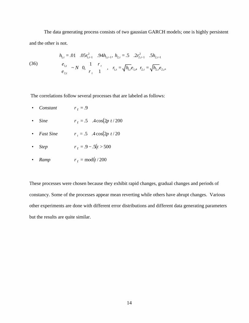
The data generating process consists of two gaussian GARCH models; one is highly persistent

and the other is not.

(36)

2 21, 1, 1 1, 1 2, 2, 1 2, 1

1,1, 1, 1, 2, 2, 2,

2,

.01 .05 .94 , .5 .2 .5

1~ 0, , , ,

1

ε ρε ε

ε ρ

− − − −= + + = + +

= =

t t t t t t

t tt t t t t t

t t

h r h h r h

N r h r h

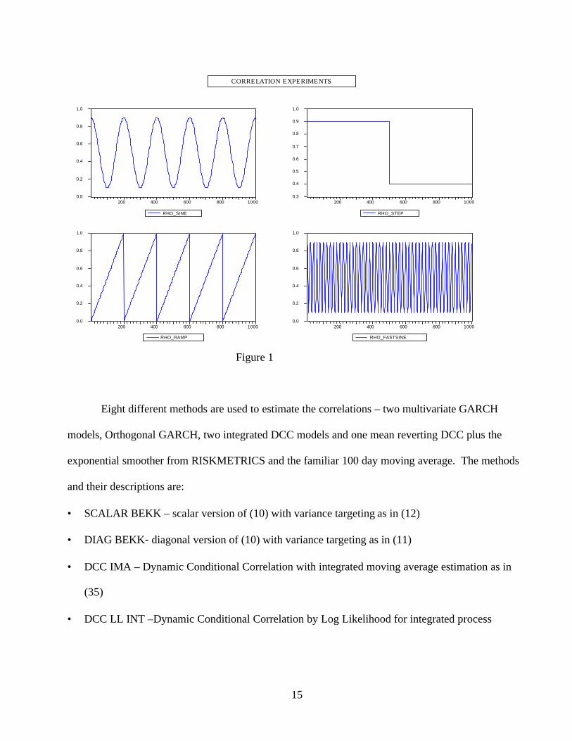
The correlations follow several processes that are labeled as follows:

• Constant 9.=tρ

• Sine ( )200/2cos4.5. tt πρ +=

• Fast Sine ( )20/2cos4.5. tt πρ +=

• Step ( )5005.9. >−= ttρ

• Ramp ( )200/mod tt =ρ

These processes were chosen because they exhibit rapid changes, gradual changes and periods of

constancy. Some of the processes appear mean reverting while others have abrupt changes. Various

other experiments are done with different error distributions and different data generating parameters

but the results are quite similar.

15

Figure 1

Eight different methods are used to estimate the correlations – two multivariate GARCH

models, Orthogonal GARCH, two integrated DCC models and one mean reverting DCC plus the

exponential smoother from RISKMETRICS and the familiar 100 day moving average. The methods

and their descriptions are:

• SCALAR BEKK – scalar version of (10) with variance targeting as in (12)

• DIAG BEKK- diagonal version of (10) with variance targeting as in (11)

• DCC IMA – Dynamic Conditional Correlation with integrated moving average estimation as in

(35)

• DCC LL INT –Dynamic Conditional Correlation by Log Likelihood for integrated process

0.0

0.2

0.4

0.6

0.8

1.0

200 400 600 800 1000

RHO_SINE

0.3

0.4

0.5

0.6

0.7

0.8

0.9

1.0

200 400 600 800 1000

RHO_STEP

0.0

0.2

0.4

0.6

0.8

1.0

200 400 600 800 1000

RHO_RAMP

0.0

0.2

0.4

0.6

0.8

1.0

200 400 600 800 1000

RHO_FASTSINE

CORRELATION EXPERIMENTS

16

• DCC LL MR – Dynamic Conditional Correlation by Log Likelihood with mean reverting model

as in (18)

• MA100- Moving Average of 100 days

• EX .06 –Exponential smoothing with parameter=.06

• OGARCH- orthogonal GARCH or principle components GARCH as in (8).

Three performance measures are used. The first is simply the comparison of the estimated

correlations with the true correlations by mean absolute error. This is defined as:

(37) ∑ −= ttTMAE ρρ

1

and of course the smallest values are the best. A second measure is a test for autocorrelation of the

squared standardized residuals. For a multivariate problem, the standardized residuals are defined as

(38) ttt rH 2/1−=ν

which in this bivariate case is implemented with a triangular square root defined as:

(39)

( ) ( )2,11

,12

,22

,2,2

,11,1,1

ˆ1

ˆ

ˆ1

1

/

tt

tt

tt

tt

ttt

Hr

Hr

Hr

ρ

ρ

ρν

ν

−−

−=

=

The test is computed as an F test from the regression of 2,1 tν and 2

,2 tν on 5 lags of the squares and

cross products of the standardized residuals plus an intercept. The number of rejections using a 5%

critical value is a measure of the performance of the estimator since the more rejections, the more

evidence that the standardized residuals have remaining time varying volatilities. This test can

obviously be used for real data.

17

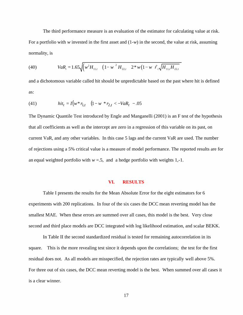
The third performance measure is an evaluation of the estimator for calculating value at risk.

For a portfolio with w invested in the first asset and (1-w) in the second, the value at risk, assuming

normality, is

(40) ( ) ( )( )2211, 22, 11, 22,ˆ1.65 1 2* 1t t t t t tVaR w H w H w w H Hρ= + − + −

and a dichotomous variable called hit should be unpredictable based on the past where hit is defined

as:

(41) ( )( ) 05.*1* ,2,1 −−<−+= tttt VaRrwrwIhit

The Dynamic Quantile Test introduced by Engle and Manganelli (2001) is an F test of the hypothesis

that all coefficients as well as the intercept are zero in a regression of this variable on its past, on

current VaR, and any other variables. In this case 5 lags and the current VaR are used. The number

of rejections using a 5% critical value is a measure of model performance. The reported results are for

an equal weighted portfolio with w =.5, and a hedge portfolio with weights 1,-1.

VI. RESULTS

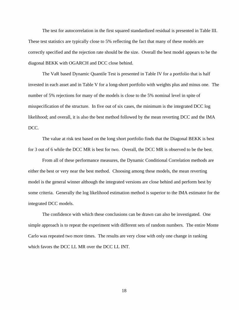
Table I presents the results for the Mean Absolute Error for the eight estimators for 6

experiments with 200 replications. In four of the six cases the DCC mean reverting model has the

smallest MAE. When these errors are summed over all cases, this model is the best. Very close

second and third place models are DCC integrated with log likelihood estimation, and scalar BEKK.

In Table II the second standardized residual is tested for remaining autocorrelation in its

square. This is the more revealing test since it depends upon the correlations; the test for the first

residual does not. As all models are misspecified, the rejection rates are typically well above 5%.

For three out of six cases, the DCC mean reverting model is the best. When summed over all cases it

is a clear winner.

18

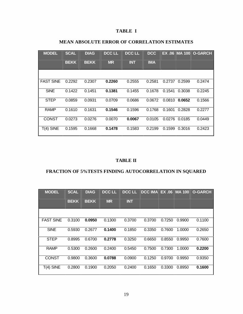
The test for autocorrelation in the first squared standardized residual is presented in Table III.

These test statistics are typically close to 5% reflecting the fact that many of these models are

correctly specified and the rejection rate should be the size. Overall the best model appears to be the

diagonal BEKK with OGARCH and DCC close behind.

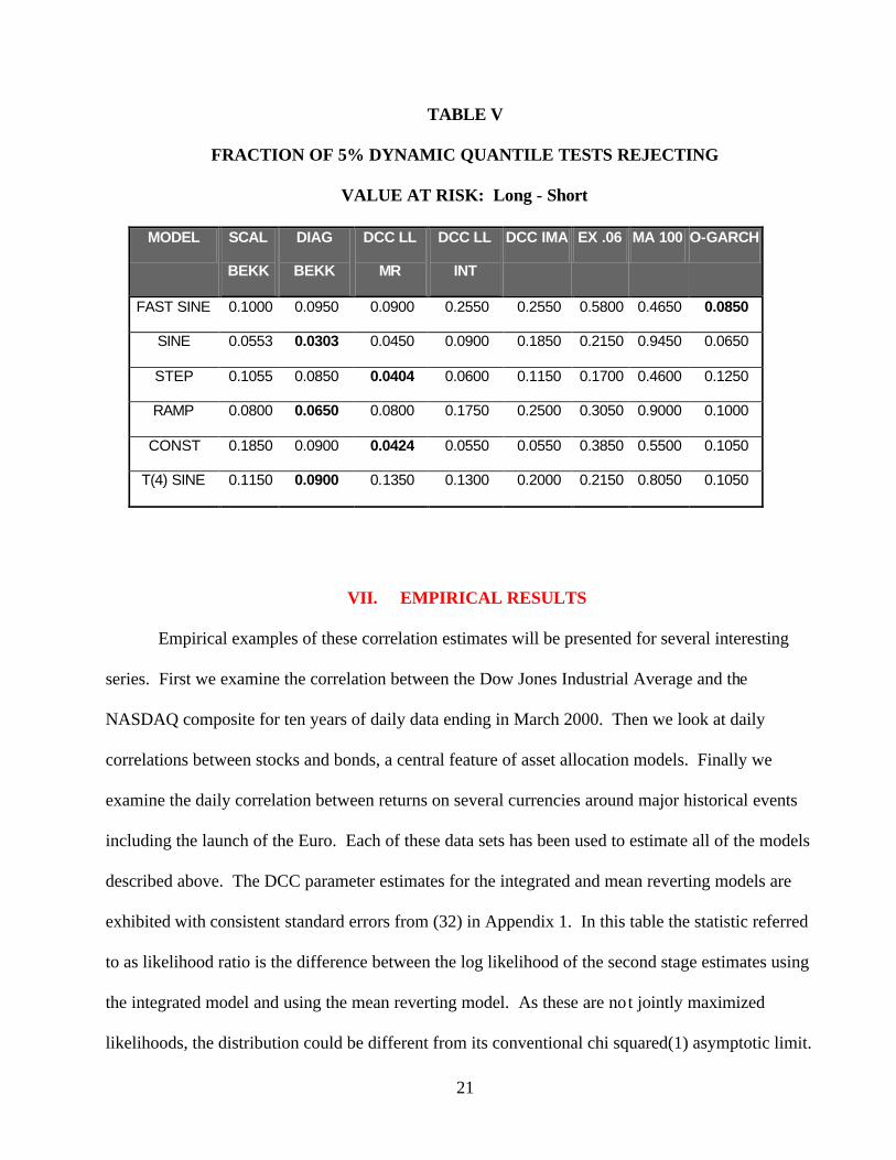
The VaR based Dynamic Quantile Test is presented in Table IV for a portfolio that is half

invested in each asset and in Table V for a long-short portfolio with weights plus and minus one. The

number of 5% rejections for many of the models is close to the 5% nominal level in spite of

misspecification of the structure. In five out of six cases, the minimum is the integrated DCC log

likelihood; and overall, it is also the best method followed by the mean reverting DCC and the IMA

DCC.

The value at risk test based on the long short portfolio finds that the Diagonal BEKK is best

for 3 out of 6 while the DCC MR is best for two. Overall, the DCC MR is observed to be the best.

From all of these performance measures, the Dynamic Conditional Correlation methods are

either the best or very near the best method. Choosing among these models, the mean reverting

model is the general winner although the integrated versions are close behind and perform best by

some criteria. Generally the log likelihood estimation method is superior to the IMA estimator for the

integrated DCC models.

The confidence with which these conclusions can be drawn can also be investigated. One

simple approach is to repeat the experiment with different sets of random numbers. The entire Monte

Carlo was repeated two more times. The results are very close with only one change in ranking

which favors the DCC LL MR over the DCC LL INT.

19

TABLE I

MEAN ABSOLUTE ERROR OF CORRELATION ESTIMATES

MODEL SCAL

BEKK

DIAG

BEKK

DCC LL

MR

DCC LL

INT

DCC

IMA

EX .06 MA 100 O-GARCH

FAST SINE 0.2292 0.2307 0.2260 0.2555 0.2581 0.2737 0.2599 0.2474

SINE 0.1422 0.1451 0.1381 0.1455 0.1678 0.1541 0.3038 0.2245

STEP 0.0859 0.0931 0.0709 0.0686 0.0672 0.0810 0.0652 0.1566

RAMP 0.1610 0.1631 0.1546 0.1596 0.1768 0.1601 0.2828 0.2277

CONST 0.0273 0.0276 0.0070 0.0067 0.0105 0.0276 0.0185 0.0449

T(4) SINE 0.1595 0.1668 0.1478 0.1583 0.2199 0.1599 0.3016 0.2423

TABLE II

FRACTION OF 5%TESTS FINDING AUTOCORRELATION IN SQUARED

MODEL SCAL

BEKK

DIAG

BEKK

DCC LL

MR

DCC LL

INT

DCC IMA EX .06 MA 100 O-GARCH

FAST SINE 0.3100 0.0950 0.1300 0.3700 0.3700 0.7250 0.9900 0.1100

SINE 0.5930 0.2677 0.1400 0.1850 0.3350 0.7600 1.0000 0.2650

STEP 0.8995 0.6700 0.2778 0.3250 0.6650 0.8550 0.9950 0.7600

RAMP 0.5300 0.2600 0.2400 0.5450 0.7500 0.7300 1.0000 0.2200

CONST 0.9800 0.3600 0.0788 0.0900 0.1250 0.9700 0.9950 0.9350

T(4) SINE 0.2800 0.1900 0.2050 0.2400 0.1650 0.3300 0.8950 0.1600

20

STANDARDIZED SECOND RESIDUAL

TABLE III

FRACTION OF 5% TESTS FINDING AUTOCORRELATION IN SQUARED

STANDARDIZED FIRST RESIDUAL

TABLE IV

FRACTION OF 5% DYNAMIC QUANTILE TESTS REJECTING

VALUE AT RISK: Equal Weighted

MODEL SCAL

BEKK

DIAG

BEKK

DCC LL

MR

DCC LL

INT


FAST SINE 0.0300 0.0450 0.0350 0.0300 0.0450 0.2450 0.4350 0.1200

SINE 0.0452 0.0556 0.0250 0.0350 0.0350 0.1600 0.4100 0.3200

STEP 0.1759 0.1650 0.0758 0.0650 0.0800 0.2450 0.3950 0.6100

RAMP 0.0750 0.0650 0.0500 0.0400 0.0450 0.2000 0.5300 0.2150

CONST 0.0600 0.0800 0.0667 0.0550 0.0550 0.2600 0.4800 0.2650

T(4) SINE 0.1250 0.1150 0.1000 0.0850 0.1200 0.1950 0.3950 0.2050

MODEL SCAL

BEKK

DIAG

BEKK

DCC LL

MR

DCC LL

INT


FAST SINE 0.2250 0.0450 0.0600 0.0600 0.0650 0.0750 0.6550 0.0600

SINE 0.0804 0.0657 0.0400 0.0300 0.0600 0.0400 0.6250 0.0400

STEP 0.0302 0.0400 0.0505 0.0500 0.0450 0.0300 0.6500 0.0250

RAMP 0.0550 0.0500 0.0500 0.0600 0.0600 0.0650 0.7500 0.0400

CONST 0.0200 0.0250 0.0242 0.0250 0.0250 0.0400 0.6350 0.0150

T(4) SINE 0.0950 0.0550 0.0850 0.0800 0.0950 0.0850 0.4900 0.1050

21

TABLE V

FRACTION OF 5% DYNAMIC QUANTILE TESTS REJECTING

VALUE AT RISK: Long - Short

MODEL SCAL

BEKK

DIAG

BEKK

DCC LL

MR

DCC LL

INT


FAST SINE 0.1000 0.0950 0.0900 0.2550 0.2550 0.5800 0.4650 0.0850

SINE 0.0553 0.0303 0.0450 0.0900 0.1850 0.2150 0.9450 0.0650

STEP 0.1055 0.0850 0.0404 0.0600 0.1150 0.1700 0.4600 0.1250

RAMP 0.0800 0.0650 0.0800 0.1750 0.2500 0.3050 0.9000 0.1000

CONST 0.1850 0.0900 0.0424 0.0550 0.0550 0.3850 0.5500 0.1050

T(4) SINE 0.1150 0.0900 0.1350 0.1300 0.2000 0.2150 0.8050 0.1050

VII. EMPIRICAL RESULTS

Empirical examples of these correlation estimates will be presented for several interesting

series. First we examine the correlation between the Dow Jones Industrial Average and the

NASDAQ composite for ten years of daily data ending in March 2000. Then we look at daily

correlations between stocks and bonds, a central feature of asset allocation models. Finally we

examine the daily correlation between returns on several currencies around major historical events

including the launch of the Euro. Each of these data sets has been used to estimate all of the models

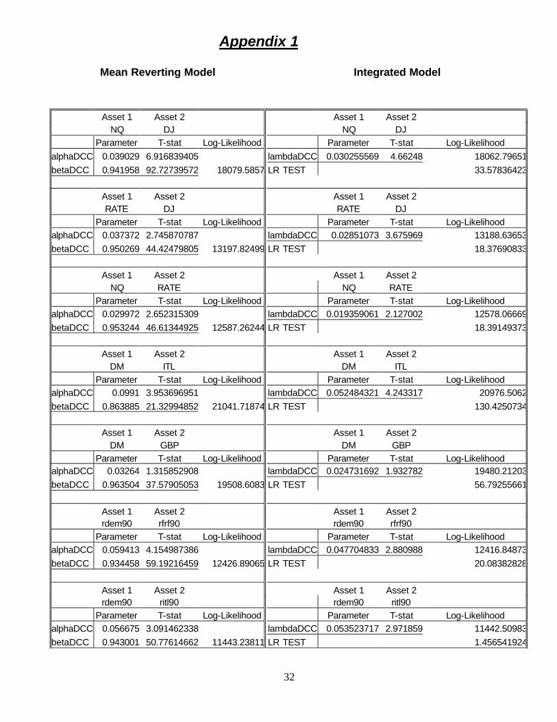
described above. The DCC parameter estimates for the integrated and mean reverting models are

exhibited with consistent standard errors from (32) in Appendix 1. In this table the statistic referred

to as likelihood ratio is the difference between the log likelihood of the second stage estimates using

the integrated model and using the mean reverting model. As these are not jointly maximized

likelihoods, the distribution could be different from its conventional chi squared(1) asymptotic limit.

22

Furthermore, non-normality of the returns would also affect this limiting distribution. A. Dow Jones

and Nasdaq.

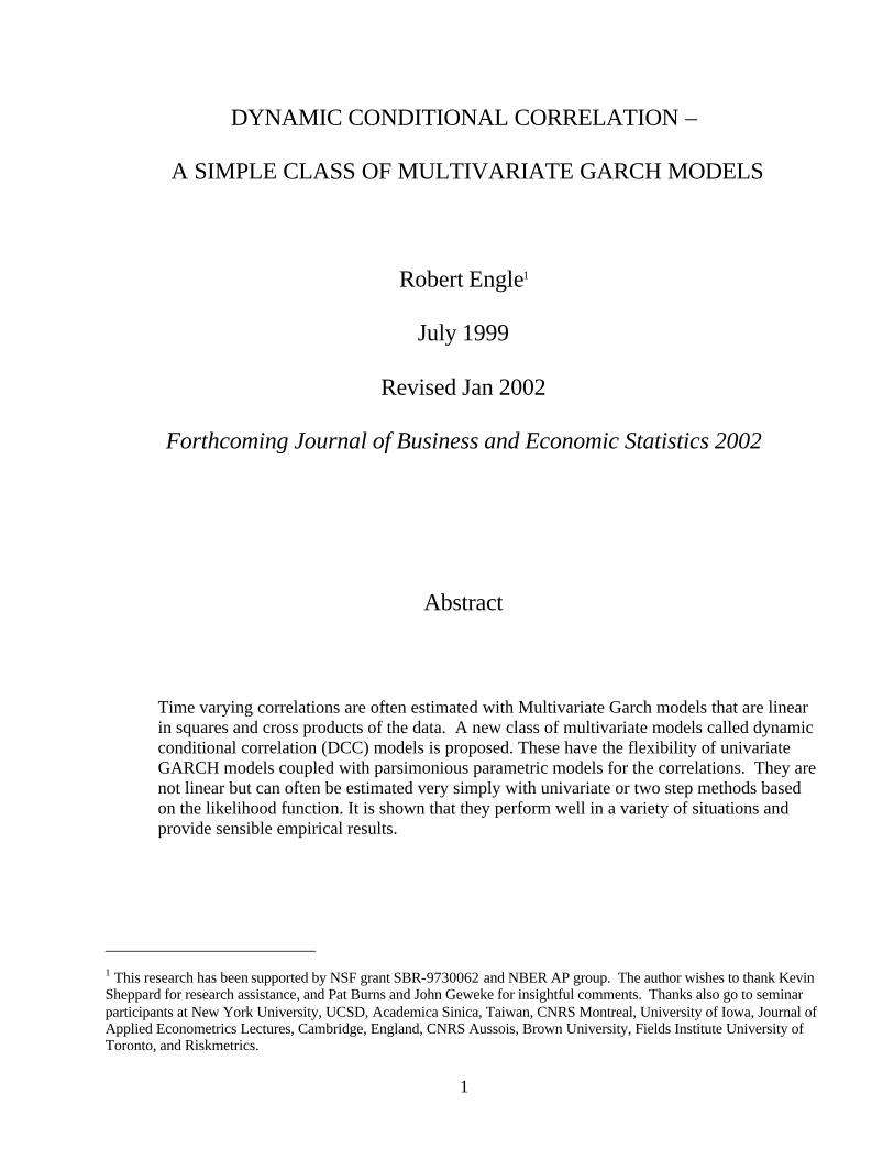
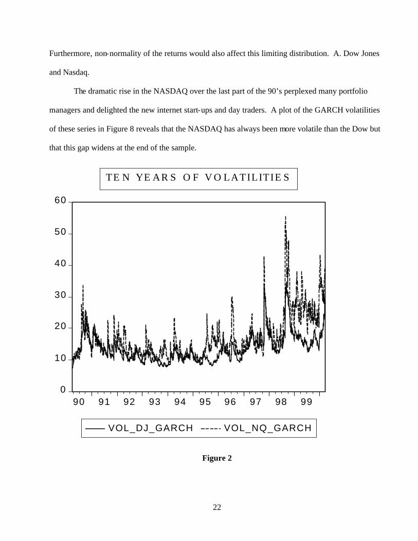
The dramatic rise in the NASDAQ over the last part of the 90’s perplexed many portfolio

managers and delighted the new internet start-ups and day traders. A plot of the GARCH volatilities

of these series in Figure 8 reveals that the NASDAQ has always been more volatile than the Dow but

that this gap widens at the end of the sample.

0

10

20

30

40

50

60

90 91 92 93 94 95 96 97 98 99

VOL_DJ_GARCH VOL_NQ_GARCH

TEN YEA RS OF V OLATILITIES

Figure 2

23

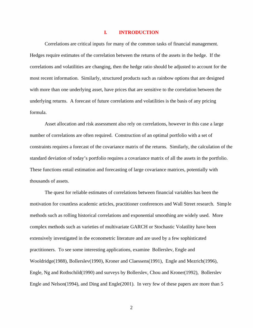
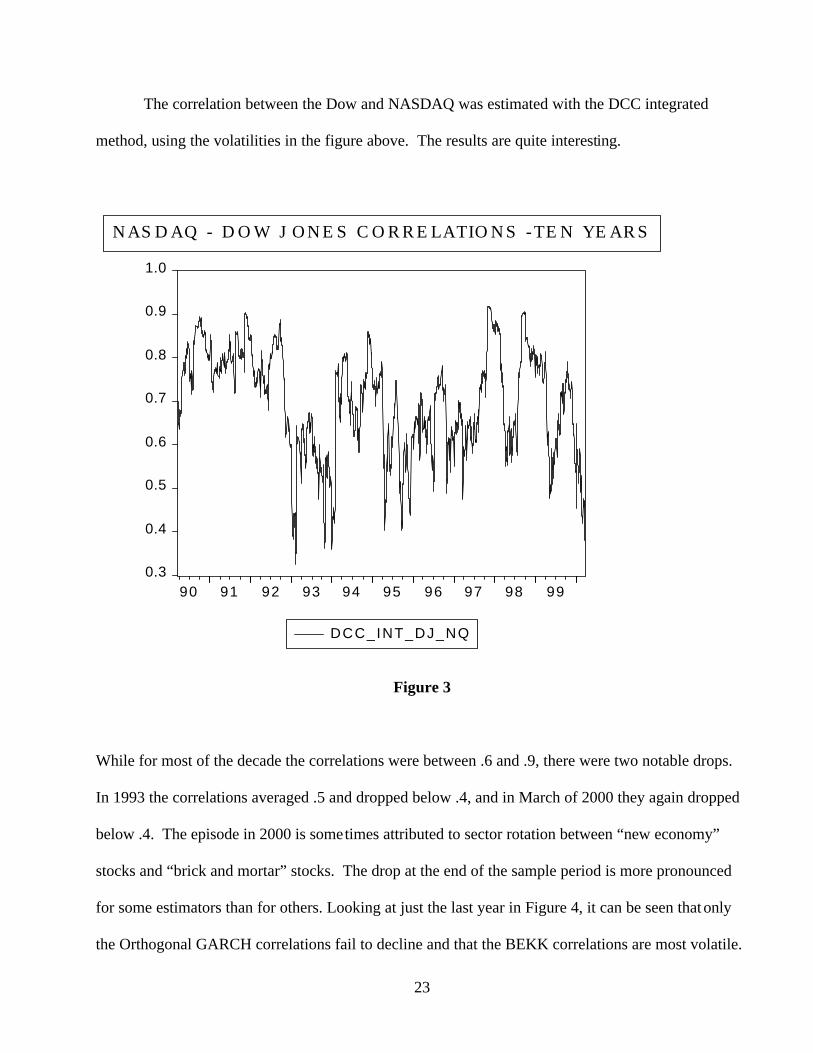
The correlation between the Dow and NASDAQ was estimated with the DCC integrated

method, using the volatilities in the figure above. The results are quite interesting.

0.3

0.4

0.5

0.6

0.7

0.8

0.9

1.0

90 91 92 93 94 95 96 97 98 99

DCC_INT_DJ_NQ

NASDAQ - DOW JONES CORRELATIONS -TEN YEARS

Figure 3

While for most of the decade the correlations were between .6 and .9, there were two notable drops.

In 1993 the correlations averaged .5 and dropped below .4, and in March of 2000 they again dropped

below .4. The episode in 2000 is sometimes attributed to sector rotation between “new economy”

stocks and “brick and mortar” stocks. The drop at the end of the sample period is more pronounced

for some estimators than for others. Looking at just the last year in Figure 4, it can be seen that only

the Orthogonal GARCH correlations fail to decline and that the BEKK correlations are most volatile.

24

. 3

.4

.5

.6

.7

.8

.9

1 9 9 9 : 0 7 1 9 9 9 : 1 0 2 0 0 0 : 0 1

D C C _ I N T _ D J _ N Q

.3

.4

.5

.6

.7

.8

.9

1 9 9 9 : 0 4 1 9 9 9 : 0 7 1 9 9 9 : 1 0 2 0 0 0 : 0 1

D C C _ M R _ D J _ N Q

.2

.3

.4

.5

.6

.7

.8

.9

1 9 9 9 : 0 7 1 9 9 9 : 1 0 2 0 0 0 : 0 1

D I A G _ B E K K _ D J _ N Q

.3

.4

.5

.6

.7

.8

1 9 9 9 : 0 4 1 9 9 9 : 0 7 1 9 9 9 : 1 0 2 0 0 0 : 0 1

O G A R C H _ D J _ N Q

C O R R E L A T IO N S 3 /1 9 9 9 T O 3 /2 0 0 0

Figure 4

B. Stocks and Bonds

The second empirical example is the correlation between domestic stocks and bonds. Taking

bond returns to be minus the change in the 30 year benchmark yield to maturity, the correlation

between bond yields and the Dow and the Nasdaq are shown in Figure 5 for the integrated DCC for

25

the last ten years. The correlations are generally positive in the range of .4 except for the summer of

1998 when they become highly negative, and the end of the sample when they are about zero. While

it is widely reported in the press that the Nasdaq does not seem to be sensitive to interest rates, the

data suggests that this is only true for some limited time periods including the first quarter of 2000,

and that this is also true for the Dow. Throughout the decade it appears that the Dow is slightly more

correlated with bond prices than is the Nasdaq.

-.6

-.4

-.2

.0

.2

.4

.6

.8

90 91 92 93 94 95 96 97 98 99

DCC_INT_DJ_BOND DCC_INT_NQ_BOND

B OND CORRELATIONS - TEN YEAR S

Figure 5

26

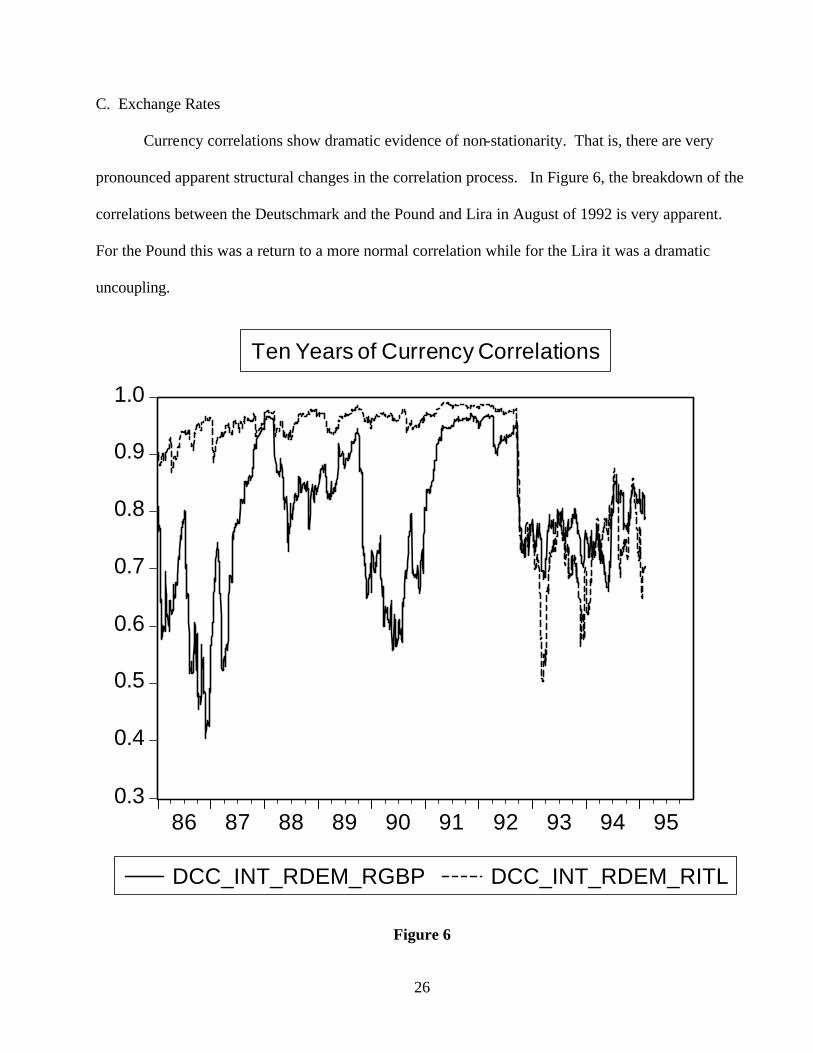
C. Exchange Rates

Currency correlations show dramatic evidence of non-stationarity. That is, there are very

pronounced apparent structural changes in the correlation process. In Figure 6, the breakdown of the

correlations between the Deutschmark and the Pound and Lira in August of 1992 is very apparent.

For the Pound this was a return to a more normal correlation while for the Lira it was a dramatic

uncoupling.

0.3

0.4

0.5

0.6

0.7

0.8

0.9

1.0

86 87 88 89 90 91 92 93 94 95

DCC_INT_RDEM_RGBP DCC_INT_RDEM_RITL

Ten Years of Currency Correlations

Figure 6

27

Figure 7 shows currency correlations leading up to the launch of the Euro in January 1999.

The Lira has lower correlations with the Franc and Deutschmark from 93 to 96 but then they

gradually approach one. As the Euro is launched, the estimated correlation has moved essentially to

one. In the last year it drops below .95 only once for the Franc/Lira and not at all for the other two

pairs.

-0.2

0.0

0.2

0.4

0.6

0.8

1.0

1994 1995 1996 1997 1998

DCC_INT_RDEM_RFRFDCC_INT_RDEM_RITL

DCC_INT_RFRF_RITL

CURRENCY CORRELATIONS

Figure 7

28

From the results in Appendix 1, it is seen that this is the only data set for which the integrated DCC

cannot be rejected against the mean reverting DCC. The non-stationarity in these correlations is

presumably responsible. It is somewhat surprising that a similar result is not found for the prior

currency pairs.

D. Testing the Empirical Models

For each of these data sets, the same set of tests can be constructed that were used in the

Monte Carlo experiment. In this case of course, the mean absolute errors cannot be observed, but the

tests for residual ARCH can be computed and the tests for value at risk can be computed. In the latter

case, the results are subject to various interpretations as the assumption of normality is a potential

source of rejection. In each case the number of observations is larger than in the Monte Carlo

experiment ranging from 1400 to 2600.

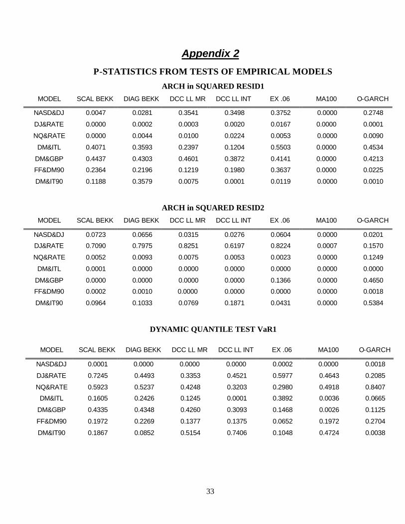
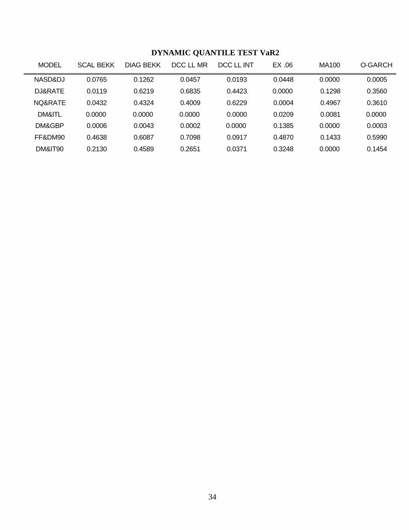
The p-statistics for each of four tests are given in Appendix 2. The tests are the tests for

residual autocorrelation in squares and for accuracy of value at risk for two portfolios. The two

portfolios are an equally weighted portfolio and a long short portfolio. They presumably are sensitive

to rather different failures of correlation estimates. From the four tables, it is immediately clear that

most of the models are misspecified for most of the data sets. If a 5% test is done for all the data sets

on each of the criteria, then the expected number of rejections for each model would be just over one

out of 28 possibilities. Across the models there are from 10 to 21 rejections at the 5% level!

Without exception, the worst performer on all of the tests and data sets is the moving average

model with 100 lags. From counting the total number of rejections, the best model is the Diagonal

BEKK with 10 rejections. The DCC LL MR, SCALAR BEKK, O_GARCH and EX .06 all have 12

29

rejections while the DCC LL INT has 14. Probably, these differences are not large enough to be

convincing.

If a 1% test is used reflecting the larger sample size, then the number of rejections ranges from

7 to 21. Again the MA 100 is the worst but now the EX .06 is the winner. The DCC LL MR , DCC

LL INT and Diag BEKK are all tied for second with 9 rejections.

The implications of this comparison are mainly that a bigger and more systematic comparison

is required. These results suggest first of all that real data is more complicated than any of these

models. Secondly, it appears that the DCC models are competitive with the other methods, some of

which are difficult to generalize to large systems.

VIII. CONCLUSIONS

In this paper a new family of multivariate GARCH models has been proposed which can be

simply estimated in two steps from univariate GARCH estimates of each equation. A Maximum

Likelihood estimator has been proposed and several different specifications suggested. The goal of

this proposal is to find specifications that potentially can estimate large covariance matrices. In this

paper, only bivariate systems have been estimated to establish the accuracy of this model for simpler

structures. However, the procedure has been carefully defined and should also work for large

systems. A desirable practical feature of the DCC models, is that multivariate and univariate

volatility forecasts are consistent with each other. When new variables are added to the system, the

volatility forecasts of the original assets will be unchanged and correlations may even remain

unchanged depending upon how the model is revised.

30

The main finding in this paper is that the bivariate version of this model provides a very good

approximation to a variety of time varying correlation processes. The comparison of DCC with

simple multivariate GARCH and several other estimators shows that the DCC is often the most

accurate. This is true whether the criterion is mean absolute error, diagnostic tests or tests based on

value at risk calculations.

Empirical examples from typical financial applications are quite encouraging as they reveal

important time varying features that might otherwise be difficult to quantify. Statistical tests on real

data indicate that all of these models are misspecified but that the DCC models are competitive with

the multivariate GARCH specifications and superior to moving average methods.

31

REFERENCES

Alexander, C.O. (1998), “Volatility and Correlation: Methods, Models and Applications,” in Risk

Manangement and Analysis: Measuring and Modelling Financial Risk(C.O. Alexander, Ed. )

Wiley.

Alexander, C.O. (2001), “Orthogonal GARCH,” Mastering Risk (C.O. Alexander, Ed.) Volume 2.

Financial Times – Prentice Hall pp21-38.

Bollerslev, Tim (1990), “Modeling the Coherence in Short-run Nominal Exchange Rates: A

Multivariate Generalized ARCH Model,” Review of Economics and Statistics, 72:498-505.

Bollerslev, Tim, Robert Engle and J.M. Wooldridge (1988) “A Capital Asset Pricing Model with

Time Varying Covariances," Journal of Political Economy 96, 116-131.

Bollerslev, Tim, Robert Engle and D. Nelson (1994), “ARCH Mod Handbook of Econometrics,

Volume IV, (ed. R. Engle and D. McFadden), (Amsterdam, North Holland), 2959-3038.

Ding, Zhuanxin and Robert Engle (2001), “Large Scale Conditional Covariance Matrix Modeling,

Estimation and Testing,” Academia Economic Papers, 29,2 pp157-184.

Engle, Robert and K. Kroner (1995), "Multivariate Simultaneous GARCH," Econometric Theory 11,

122-150.

Engle, Robert and Joseph Mezrich (1996), “GARCH for Groups,” Risk August, Vol. 9, No. 8: pp 36-

40.

Engle, Robert and Simone Manganelli (1999), “CAViaR: Conditional Value At Risk By Regression

Quantiles,” NBER Working Paper 7341.

Engle, Robert and Kevin Sheppard, (2001), “Theoretical and Empirical properties of Dynamic

Conditional Correlation Multivariate GARCH,” NBER Working Paper 8554.

Kroner, Kenneth F. and Victor K. Ng (1998), “Modeling Asymmetric Comovements of Asset

Returns,” Review of Financial Studies, pp 817-844.

Kroner, K. F. and S.Claessens (1991), “Optimal Dynamic Hedging Portfolios and the Currency

Composition of External Debt,” Journal of International Money and Finance, 10, 131-148.

Newey, Whitney and Daniel McFadden (1994), “Large Sample Estimation and Hypothesis Testing,”

Chapter 36 in Handbook of Econometrics Volume IV , (ed. Engle and McFadden), Elsevier

Science B.V. pp2113-2245.

32

Appendix 1

Mean Reverting Model Integrated Model

Asset 1 Asset 2 Asset 1 Asset 2 NQ DJ NQ DJ Parameter T-stat Log-Likelihood Parameter T-stat Log-Likelihood

alphaDCC 0.039029 6.916839405 lambdaDCC 0.030255569 4.66248 18062.79651betaDCC 0.941958 92.72739572 18079.5857 LR TEST 33.57836423

Asset 1 Asset 2 Asset 1 Asset 2 RATE DJ RATE DJ Parameter T-stat Log-Likelihood Parameter T-stat Log-Likelihood


Asset 1 Asset 2 Asset 1 Asset 2 NQ RATE NQ RATE Parameter T-stat Log-Likelihood Parameter T-stat Log-Likelihood


Asset 1 Asset 2 Asset 1 Asset 2 DM ITL DM ITL Parameter T-stat Log-Likelihood Parameter T-stat Log-Likelihood


Asset 1 Asset 2 Asset 1 Asset 2 DM GBP DM GBP Parameter T-stat Log-Likelihood Parameter T-stat Log-Likelihood


Asset 1 Asset 2 Asset 1 Asset 2 rdem90 rfrf90 rdem90 rfrf90 Parameter T-stat Log-Likelihood Parameter T-stat Log-Likelihood


Asset 1 Asset 2 Asset 1 Asset 2 rdem90 ritl90 rdem90 ritl90 Parameter T-stat Log-Likelihood Parameter T-stat Log-Likelihood


33

Appendix 2

P-STATISTICS FROM TESTS OF EMPIRICAL MODELS

ARCH in SQUARED RESID1

MODEL SCAL BEKK DIAG BEKK DCC LL MR DCC LL INT EX .06 MA100 O-GARCH

NASD&DJ 0.0047 0.0281 0.3541 0.3498 0.3752 0.0000 0.2748

DJ&RATE 0.0000 0.0002 0.0003 0.0020 0.0167 0.0000 0.0001

NQ&RATE 0.0000 0.0044 0.0100 0.0224 0.0053 0.0000 0.0090

DM&ITL 0.4071 0.3593 0.2397 0.1204 0.5503 0.0000 0.4534

DM&GBP 0.4437 0.4303 0.4601 0.3872 0.4141 0.0000 0.4213

FF&DM90 0.2364 0.2196 0.1219 0.1980 0.3637 0.0000 0.0225

DM&IT90 0.1188 0.3579 0.0075 0.0001 0.0119 0.0000 0.0010

ARCH in SQUARED RESID2


NASD&DJ 0.0723 0.0656 0.0315 0.0276 0.0604 0.0000 0.0201

DJ&RATE 0.7090 0.7975 0.8251 0.6197 0.8224 0.0007 0.1570

NQ&RATE 0.0052 0.0093 0.0075 0.0053 0.0023 0.0000 0.1249

DM&ITL 0.0001 0.0000 0.0000 0.0000 0.0000 0.0000 0.0000

DM&GBP 0.0000 0.0000 0.0000 0.0000 0.1366 0.0000 0.4650

FF&DM90 0.0002 0.0010 0.0000 0.0000 0.0000 0.0000 0.0018

DM&IT90 0.0964 0.1033 0.0769 0.1871 0.0431 0.0000 0.5384

DYNAMIC QUANTILE TEST VaR1


NASD&DJ 0.0001 0.0000 0.0000 0.0000 0.0002 0.0000 0.0018

DJ&RATE 0.7245 0.4493 0.3353 0.4521 0.5977 0.4643 0.2085

NQ&RATE 0.5923 0.5237 0.4248 0.3203 0.2980 0.4918 0.8407

DM&ITL 0.1605 0.2426 0.1245 0.0001 0.3892 0.0036 0.0665

DM&GBP 0.4335 0.4348 0.4260 0.3093 0.1468 0.0026 0.1125

FF&DM90 0.1972 0.2269 0.1377 0.1375 0.0652 0.1972 0.2704

DM&IT90 0.1867 0.0852 0.5154 0.7406 0.1048 0.4724 0.0038

34

DYNAMIC QUANTILE TEST VaR2


NASD&DJ 0.0765 0.1262 0.0457 0.0193 0.0448 0.0000 0.0005

DJ&RATE 0.0119 0.6219 0.6835 0.4423 0.0000 0.1298 0.3560

NQ&RATE 0.0432 0.4324 0.4009 0.6229 0.0004 0.4967 0.3610

DM&ITL 0.0000 0.0000 0.0000 0.0000 0.0209 0.0081 0.0000

DM&GBP 0.0006 0.0043 0.0002 0.0000 0.1385 0.0000 0.0003

FF&DM90 0.4638 0.6087 0.7098 0.0917 0.4870 0.1433 0.5990

DM&IT90 0.2130 0.4589 0.2651 0.0371 0.3248 0.0000 0.1454

Documents

DYNAMIC CONDITIONAL CORRELATION – A SIMPLE CLASS …archive.nyu.edu/bitstream/2451/26482/2/02-38.pdf · 1 DYNAMIC CONDITIONAL CORRELATION – A SIMPLE CLASS OF MULTIVARIATE GARCH