1

DYNAMIC BEHAVIOUR OF HIGH SPEED RAILWAY BRIDGES USING PRECAST RC GIRDERS

Narciso Jorge Ferreira

Abstract

In recent years, we have been assisting to increasing speeds in the HS area, and such fact causes new problems on dynamic behaviour of bridges that do not happen for lower speeds. Resonance is one phenomenon that usually arises when trains reach speeds over 200km/h. The objective of this work is to study the dynamic response of one viaduct composed by precast/pre-stressed girders, when admitting structural continuity of the deck and loss of bending stiffness due to cracking that appears on support sections when there is no prescribed pre-stressed connection.

Two finite element models were created, allowing the simulation of the structural system in order to obtain the dynamic response. Comparisons between the models were made, calculating the dynamic responses for train speeds between 140km/h and 420km/h.

Keywords: Precast/Pre-stressed girders, high speed railway bridges, dynamic behaviour, evolutive structures.

1 Introduction

The construction of high speed railway lines has some specifications on its design, such as theoretical line, vehicles, and track quality and, most important, dynamic response. A resonance phenomenon appears when trains reach speeds over 200km/h. This phenomenon occurs due to the regular forces transmitted to the deck that originates an excitation frequency equal to the natural frequency of the bridge.

In this article, the results obtained from the study will be presented with the objective of registering the implications that viaducts built by precast/pre-stressed girders have in the dynamic response. This type of construction has differences in the design methodology when compared with construction that uses cast-in-place concrete. These differences are related to different structural systems that this type of construction presents during its life cycle. In this paper it will be presented a methodology [11] that allows the calculation of strains in this type of construction. It was also done a description of the usual procedures to use precast/pre-stressed girders, as well as the connections for establishing structural continuity.

To study the implications that the use of pre-cast/pre-stressed girders have, the dynamic analyses are realized in one system that has full continuity

and another one where support sections have less bending stiffness due to the presence of cracking. Cracking appears due to the fact that no pre-stress is prescribed to the connection. This kind of connection is simpler when compared with a connection that uses pre-stress and, because of that, the construction speed increases.

To determine the dynamic response, two finite element models were realized and compared, one using shell elements and another one using frame elements. The dynamic response is obtained from circulating the HSLM A and real trains families between 140km/h and 420km/h.

2 Precast/Pre-stressed girders

The use of precast elements was associated for a long time to a poor construction and, thus, it wasn’t seen as a good choice. However, the construction of viaducts and bridges with precast/pre-stressed girders has some advantages that leads to increasing solutions in this field. The good quality of pieces and reduction of work time are some of the advantages of this technique.

The construction of bridges with precast/pre-stressed girders has values for slenderness that depends on his type. Railway bridges usually present values smaller than 16 while road bridges present values smaller than 20 [14]. In cross-sections, there

2

are usually adopted “I” and “U” shape girders. “U” girders present more flexural stiffness due to his inferior flange and better torsion behaviour after casting the slab.

The first structural systems uses precast/pre-stressed girders without continuity and, therefore, they work as simple supported beams. This methodology is simple and easy to perform, and its design is also very simple because there is no stress redistribution related to deformations on structures [8]. Otherwise, some problems are common in this method. Durability is one of these problems, because joints between girders are permeable and the durability of these sections reduces. Other problem is connected to the fact that these joints provoke bad comfort when vehicles cross these sections, especially in road bridges.

When continuity is established, it is performed on the support sections for simplicity issues. In fact, continuity must be established on inflection points of the deck because in this situation moments are reduced and the connection just needs to transmit shear force, but this will complicate the construction process. Two types of continuity can be defined: apparent and total.

The establishment of apparent continuity can be made by casting the slab in the support sections. This kind of proceedings resolves the problems of comfort in the previous solution and at same time allows girders to work as simply supported. This method is based on the idea that a slab do not origin restraint moments because it has a reduced thickness.

Figure 1: Example of connection done in the deck [8].

Full continuity is done by joint end-sections of girders and it is performed by casting a cross girder that can use reinforced bars or a longitudinal prestressing solution.

The continuity can bring structural advantages in spite of complicating construction speed. In a structural way, there will be stress redistribution due to long term effects of concrete that allow reducing them in the middle sections. Similar to this, the vertical deflection is also reduced and natural vertical frequency increases. In an aesthetic way, continuity also allows higher slenderness ratios.

Stress redistribution appears due to differences between initial and final structural systems. Elastic stress determined on the initial system tend to equal those obtain from the final system. This phenomenon occurs due to long term behaviour of concrete. Due to creep, support sections tend to rotate if this displacement gets free, as happens in simply support systems. In the final system, these rotations are restrained by continuity and bending moments are generated, which are negative for the girder and slab dead loads and positive for prestressing.

When continuity is established by reinforcing bars, the negative reinforcement is placed on the deck slab while the positive one is placed at the inferior level of the section. There are some proceedings to detail the positive reinforcement:

Bent-bar or bent-strand connection, overlapping bars or strands in the diaphragm;

Bow-bar connection overlapping bars in the diaphragm;

Welded connection between bars. This connection is unadvisable due to fatigue phenomena that happen in railway bridges.

Figure 2 shows the types of connections previously presented.

3

Figure 2: Different connection types [8].

Since these connections are done by reinforcing bars and did not use longitudinal prestressing, it is natural that cracks appear in support sections. At the slab, reinforcement is prescribed to control these cracks. At the inferior level of diaphragm, tensile stress may appear due to prestressing, live load and differential temperature. The implications of these stresses on the deck behaviour have been studied, and some studies can be presented. The Report 519 – Connection of simple-span precast concrete girders for continuity, developed by NCHRP [12], investigated the strength, serviceability, and continuity of connections between precast/pre-stressed concrete girders made continuous. In this study, surveys were conducted to establish the frequency of use of positive and negative moment connections and how they were constructed. The result showed that all the responses indicate that designers prescribed negative connections and a lot of them also prescribed positive connections correspond to 1,2Mcr, where Mcr is the cracking moment of cross girder. It was also analyzed the structural continuity when cracks exist on the inferior surface of diaphragm, and the conclusion pointed that continuity was assured for service loads, being reduced to values near 70% when the structure was close to collapse. Another study [15] refers that when obvious cracking exists, continuity degree was near zero. In spite of this, when there are not visible cracks, the structure behaves as continuous. This study was based in measurement and tests made on precast/pre-stressed bridges made continuous for live load. Both studies presented indicate it must be prescribed a positive connection with resistance to 1,2Mcr. If this method would not be sufficient to control cracking on support sections, other things should be done as establishing an inferior limit to girder age to avoid formation of positive moments.

The continuity that uses prestressing on cross girder is more complex to execute but has the advantage to eliminate all the problems connected to cracking. In Portugal, this kind of solution has been much applied to make continuity [3].

Prestressing can be made for different ways, such as:

High resistance pre-stress bars linking the end-sections of girders;

Straight pre-stress cables located at slab;

Post-tensioned cables with parabola curvature.

All these procedures can be applied together taking the advantages of each one.

In Figure 3 is presented a connection that uses two types of procedures indicated before. There are prescribed high resistance pre-stress bars and post-tensioned cables. When post-tensioned cables are used, the prestressing applied in factory did not need to resist to slab dead load because when this is applied there is the post-tensioned cables already.

Figure 3: Picture of connection system [1].

Evolutive structures change their structural systems and/or cross-section during service life, leading to important stress differences between initial and final instant. These differences occur due to time-dependent effects like creep and shrinkage [14]. Structures using pre-fabricated elements are affected by this phenomenon and then, pre-fabricated bridges also behave as previously mentioned.

4

To design this kind of structures, one needs to take into account the aspects mentioned before, and a methodology will be presented. Before that, some concepts related to concrete behaviour are presented.

For one concrete element, the total strain obtained in instant t, due to an constant axial loading in instant t0 - Δσc(t0) can be defined from the following equation [4]:

)()(),()(, 000 ttttttt cTcscccic (1)

Where εci(t0) represents initial strain at load instant, εcc(t,t0) the creep deformation at instant t, εcs(t) the shrinkage strain at instant t and εcT(t) the temperature strain for the same instant.

The components of equation (1) can be grouped in mechanic strain εcσ(t,t0) and non-mechanic strain εcn(t), according to loading dependence or not. This way, the following equations are obtained:

),()(),( 000 ttttt cccic (2) )()()( ttt cTcscn

(3)

In this presentation, more importance will be given to mechanic strain. The initial strain εci(t0) is given by equation (4) while creep deformation consists in multiplying the initial strain by the creep coefficient, as shown in equation (5). This creep deformation is assumed for constant loading.

0,

00

)()(tc

cci E

tt (4)

)(),(),( 00'

0 ttttt ciccc

(5)

Where Ec,t0 represents Young’s modulus at the initial instant and φ’c(t,t0) represents the modified creep coefficient, calculated from:

28.

.00

0),(),('c

tccc E

Etttt (6)

Now, mechanic strain can be presented by equation (7) for a constant load:

),()(),( 000 ttJttt cc (7)

Where J(t,t0) is the creep function that can be represented by:

0.

00

),('1),(tc

c

EttttJ

(8)

In the situation of a variable loading along time, mechanic strain can be calculated from:

t

t

c

cc

dtJ

ttJttt

0

)(),(

),()(),( 000

(9)

Where function σc(ζ) represents the stress variation during time. If that variation could be discriminated on infinitesimal variation σc.ti, the mechanic strain takes the next expression:

),(),(0

.0 i

n

iticc ttJtt

(10)

To resolve a structure where the state of stress changes along its service life, we must use equation (9) to obtain the solution. There is the possibility to solve this equation by a step-to-step methodology where the function J(t,t0) is approximated by a shape function, or by the simplified method of ageing coefficient, where it is assumed that one constant load applied during time produces a higher creep deformation than other varying during time but with the same stress load.

Figure 4: Constant (1) and variable (2) load.

5

The relation between these two creep deformations is called by ageing coefficient χ. Now, mechanic strain can be determined by expression (11), where creep deformation is multiplied by χ.

0.

00

000

),('1),(

),()(),(

tcc

cc

Ett

tt

ttJttt

(11)

With the definitions presented here, it is possible to obtain the stress during the structure period of life. The ideas behind these expressions can be found in [11].

1,2,1

11,, )(1

'jj

efjj MMMM

(12)

iief

ii ,1,21

1,1, )(1

'

(13)

21

10,1

1'1)'1(1

RRR

(14)

2110,1 ')'1( (15)

Where numbers 1 and 2 correspond to initial and final structural system, respectively. Δφ’1 represents creep occurring in the primary element after changing the structural system and it is given by equation (16); [1+(χφ)1]ef represents the fact that stress variations occurs during time, given by expression (17).

),('),('' 011111 tttt (16)

1

0

.1

.11111 ),('),(1)'(1

t

tef E

Etttt

(17)

3 Dynamic analysis methodologies

The circulation of high speed railway vehicles provokes dynamic effects on bridges that had been studied for a long time. The increase of velocity that witnessed nowadays, has originated vertical displacements and accelerations corresponding to resonance phenomena that tends to appear for speeds higher than 200km/h.

Dynamic studies can be made by two methods:

Multiplying the static results by a dynamic factor;

Making a dynamic analysis.

The first method consists in the definition of a fictitious vehicle whose effects must be multiplied by a dynamic factor. In Figure 5 is presented the LM71 train and equation (18) e (19) show expressions that allow the calculation of the dynamic factor for carefully and standard maintained track respectively.

Figure 5: LM71 model [5].

67,100,182,02,0

44,122

L

(18)

00,200,173,02,0

16,233

L (19)

Figure 6: SW/0 and SW/2 models [5].

Table 1: SW/0 and SW/2 values [5].

However this method does not allow taking the resonance effects. These effects can just be detected with a dynamic analysis, and in Figure 7 are presented the situations where it should be done.

6

Figure 7: Flow chart for determining whether a dynamic analysis is necessary [13].

When dynamic analyses are needed, they must include the circulation of real trains and for international railway lines the HSLM family. The HSLM – High Speed Load Model was introduced to assure that the interoperability criterion was followed. This way, HSLM trains draw envelope effects assuring the line design is under the European rules. Within HSLM, there are two families: HSLM A and HSLM B. The second one was established because the first didn’t contain the effects in simple span bridges with less than 7m.

Figure 8: HSLM A model.

Figure 9: HSLM B model.

The characteristic values for both models can be found in [5].

When a dynamic analysis is necessary, the structural design must be done for the most unfavourable situation:

RTou

HSLM

dyn 2'''1 (20)

Or

)0/""71( SWLM (21) Where:

1max' stat

dyndyn y

y (22)

Safety criteria must be respected and, thus, the maximum permitted peak values of bridge deck acceleration calculated along track shall not exceed the following design values: 3,5m/s2 for ballasted tracks and 5,0m/s2 for direct fastened decks with track and structural elements designed for high speed traffic. The comfort criteria are related to passengers and like that they depend on the vertical acceleration bv inside the coach. For very good, good and acceptable level of comfort we have, respectively, 1,0m/s2, 1,3m/s2 e 2,0m/s2. This procedure has the inconvenient of realizing a dynamic analysis with bridge-train interaction. To eliminate this inconvenient, an evaluation of comfort criteria can be done by Figure 10.

Figure 10: Maximum permissible vertical deflection corresponding to vertical acceleration bv=1,0m/s2.

Dynamic analysis methodologies can be grouped by type, namely: analytical, numerical and simplified.

7

Analytical methodologies have the advantage to understanding expressions and principles that rule the dynamic response. As disadvantage, it has the fact that theoretical formulation is very complex and as consequence only simple structures can be analyzed by this procedure. The most simple model consist on a simple supported beam, with bending stiffness EI, mass per unit length µ and damping circular frequency ωd.

Figure 11: Simple supported beam.

The equation that rules this system behaviour is presented on the next expression [9]:

N

nnnn

d

Fxxt

ttxu

ttxu

xtxuEI

1

2

4

4

)()(

),(2),(),(

(23)

Where u(x,t) represents vertical displacement in order to length and time, εn(t) represents the Heaviside function and δ(x) the Dirac function. The solution of this equation is presented below by expression (24).

Lxj

TthTtftthttf

jFFutxu

j

N

n nnj

nnn

sin

)()()1(

)()(),(

1 1

210

(24)

From this equation, is now possible to obtain the expression of bending moment by making a double derivation in order to space, and it is also possible to obtain the expression for acceleration making a double derivation too in order to time.

Numerical methods allow the resolution of more complex systems in a structural and real way. These ones are mainly composed by two types: train simulated by a group of moving loads that travel on bridge; consideration of train-bridge interaction, simulating the elements of train like coaches, bogies and axles using damped elastics systems. The second methodology presented is more complex but has much more realism and gives the opportunity to determine accelerations on coaches and obtain from a direct way the level of comfort passenger. In spite of this, both methods are founded in resolution of the motion equation (25), having differences just in the degree of freedom.

)()()()( tFtKutuCtuM (25)

The moving loads method consists in creating load cases for each joint of the load path as a function of time. With vector F(t) defined, the resolution of equation (25) is done by direct integration or mode superposition.

Figure 12: Moving loads.

In the field of methods that use train-bridge interaction, different models with different degrees of complexity can be made. In Figure 13 is presented a model where the different components of train are discriminated like secondary suspension, bogies, wheels and the elastic connection between wheel and rail.

8

Figure 13: Train-bridge interaction model [6].

This system resolution is based on the solution of equation (26), where the items p and c are referred to bridge and train respectively. The method used to resolve this system uses the integration at each step and try to equal the displacements between train and bridge.

)()(

)()(

00

)()(

00

)()(

00

tFtF

tutu

KK

tutu

CC

tutu

MM

c

p

c

p

c

p

c

p

c

p

c

p

c

p

(26)

The simplified methodologies that will be presented here are called the Decomposition of Excitation at Resonance – DER, and the Residual Influence Line –LIR. In both situations is only possible to obtain the dynamic response in simple supported beams.

The DER method will over-estimate the acceleration because it is established an upper bound for response due to the simplifications introduced by this methodology. This method can be resumed to three steps that can be explained as the reduction of a multiple degree of freedom to only one degree, followed by excitation presented by a Fourier series and at last by the consideration only the term of resonance to obtain the response. All analytical steps can be found in [2], [10] e [13]. The solution obtained is presented in equation (27) and can be simplified by the multiplication of three terms (28).

)(2

2

1

2

1

2*

2

1

22cos

)(12

cos8

)(

Lx

N

k

kk

kN

kk

N

o

N

e

xsenF

xF

xLL

L

L

Kf

ty

(27)

)()()( GLACty t (28)

Where Ct represents a constant term, A(L/λ) stands for the dynamic influence line and G(λ) is a factor relative to train called train spectrum.

The LIR method has its beginning in vibration analysis due to a moving load that crosses a Bernoulli beam. Vibrations can be separated in two phases: the first one includes the time range while load is in circulation and the second phase, analyzes vibrations that happen after the load leaves the beam [2]. The simplifications adopted in this method are based in the fact that the train is very long when compared with bridge length and the maximum dynamic response happens when the last load leaves the bridges. To obtain the dynamic response of all loads that form a train, it is used the superposition of each response and expression (29), allowing the calculation of the final response. The principles that rule this equation can be found in [2], [10] e [13].

0)(

22cos

cos2111

)(

0

2

1

22

1

2

2

20

*2

esen

exsenFexF

er

eMr

rty

N

i

xi

i

N

i

xi

i

rr

ii (29)

This equation can be simplified on the multiplication of three terms and its aspect change to:

)()(max GrACy desl (30)

Where Cdesl is constant, A(r) is relative to influence line and only depends from bridge parameters and

9

G(λ) refers to effects due to moving loads over the bridge.

4 Analysis of a high speed railway viaduct

The studied viaduct presents 205,9m of length and is composed by six spans, having the middle ones a length of 28,95m while the end spans have a length of 37m. The cross-section corresponds to a double track composed with two precast/pre-stressed girders with 2,50m height that support a slab with 0,30m thickness and 14,00m width. The concrete used in the slab is the C30/37 while to the girder is the C50/60. The A500NR is used to reinforcing and the A1670/1860 is used to prestressing.

4.1 Static Analysis

To determine the dynamic differences between a precast and cast in situ solution, it was realized the evolutive methodology presented in Point 2 and developed by [11]. This process allows the effective bending stiffness calculation of the support section.

This way, the constructive process was simplified to condense the structure life in two instants: the first one is instant t0 and corresponds to fabrication time and its dead load and prestressing are the loads applied; the second instant is t1 and is related to the instant when continuity is established. For cross-sections, are defined ones with small differences to consider the different loads and instants of time. This way, the following cross-sections are defined:

Cross-section

1

Precast/Pre-stressed girder

Used for systems analysis loaded in t0;

Cross-section

2

Precast/Pre-stressed girder +

Slab

Used for evolutive systems analysis loaded in t0;

corresponds to evolution of cross-section 1;

Cross-section

3

Precast/Pre-stressed girder

Used for systems analysis loaded in t1;

Cross-section

4

Precast/Pre-stressed girder +

Slab

Used for evolutives systems analysis loaded in t1;

corresponds to evolution of cross-section 3;

Cross-section

5

Precast/Pre-stressed girder +

Slab

Non evolutive loads analysis; homogenization done with Ecm;

Table 2: Cross-sections used.

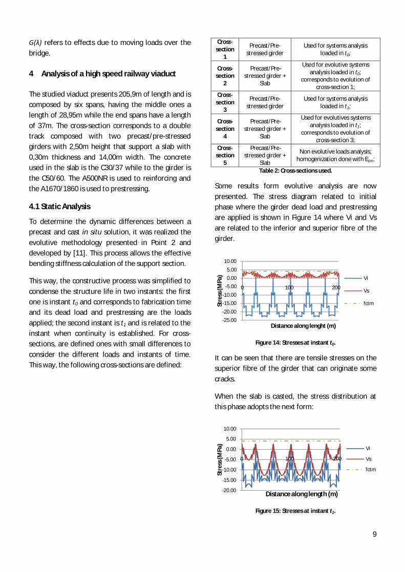
Some results form evolutive analysis are now presented. The stress diagram related to initial phase where the girder dead load and prestressing are applied is shown in Figure 14 where Vi and Vs are related to the inferior and superior fibre of the girder.

Figure 14: Stresses at instant t0.

It can be seen that there are tensile stresses on the superior fibre of the girder that can originate some cracks.

When the slab is casted, the stress distribution at this phase adopts the next form:

Figure 15: Stresses at instant t1.

-25.00

-20.00

-15.00

-10.00

-5.00

0.00

5.00

10.00

0 100 200

Stre

ss (M

Pa)

Distance along lenght (m)

Vi

Vs

fctm

-20.00

-15.00

-10.00

-5.00

0.00

5.00

10.00

0 100 200

Stre

ss (M

Pa)

Distance along length (m)

Vi

Vs

fctm

10

It is verified that the tensile stress on the superior fibre of the previous phase has passed to compressive stress due to slab dead load. The inferior fibre has reduced its level of compression because the same load provokes tensile stress in that fibre.

It is now presented the final diagram related to the characteristic combination, where it can be seen that the inferior fibre presents, in all its length, a compressive stress - Figure 16. This way, it is also verified that cracking will not appear at inferior fibres on support sections due to positive moments originated by prestressing, live load and temperature.

Figure 16: Stress (Vi) for characteristic combination.

Figure 17: Stress (Ls) for characteristic combination.

Figure 17 shows the stress values related to superior fibres of slab and it can be seen that, at the supports, the tensile stress is higher than the concrete resistance. This way, some cracking will appear at these sections and the bending stiffness related to characteristic combination will be calculated to perform the dynamic analyses.

4.2 Dynamic models and analyses

To realize the dynamic analyses of the viaduct, two finite elements models in SAP2000 were considered.

The first model uses shell elements – shell model, while the second one uses frame elements – grid model. Models are also analyzed by comparing their modal and dynamic behaviour. The Young’s modulus is affected by a factor related to the fact that the action of trains circulating over the bridge is a fast load [7]. This way, to the girder is adopted 38,5GPa and for the slab is 34,1GPa.

Figure 18: Shell model.

Figure 19: Grid model.

The modal comparison is realized by the frequencies values and their vibration mode shapes. For the frequencies, Figure 20 shows the relation between the two models.

Figure 20: Frequency comparison.

As for vibration mode shapes, a comparison can be made by the factor MAC – Modal Assurance Criterion, and this procedure gives a value between 0 and 1 for the level of compatibility between two mode shapes.

n

i

Grelhai

TGrelhai

n

i

Cascai

TCascai

n

i

Grelhai

TCascai

MAC

11

2

1

(31)

-30.00

-20.00

-10.00

0.00

10.00

0 100 200

Stre

ss (M

Pa)

Distance along lenght (m)

Stresses Vi

Max

Min

fctm

-10.00

-5.00

0.00

5.00

10.00

0 100 200

Stre

ss (M

Pa)

Distance along length (m)

Stresses Ls

Max

Min

fctm

1º V2º V

3º V

4º V1º T 2º T 5º V

6º V 3º T 4º T

0

5

10

Freq

uenc

y H

z

Frequencies

Casca

Grelha

Mode order

11

The results obtained were the following where “V” and “T” represent respectively, vertical and torsion modes:

Shell Model

1ºV 2ºV 3ºV 4ºV 1ºT 2ºT 5ºV 6ºV 3ºT 4ºT

Grid Model

1ºV 98.89% 0.00% 0.66% 0.00% 0.00% 0.00% 0.01% 0.00% 0.00% 0.00%

2ºV 99.07% 0.00% 0.00% 0.00% 0.00% 0.00% 0.00% 0.00% 0.00%

3ºV 92.36% 0.00% 0.00% 0.00% 0.19% 0.00% 0.00% 0.00%

4ºV 95.99% 0.00% 0.00% 0.00% 0.07% 0.00% 0.00%

1ºT 91.00% 0.00% 0.00% 0.00% 7.63% 0.00%

2ºT 98.93% 0.00% 0.00% 0.00% 0.05%

5ºV 55.00% 0.00% 0.00% 0.00%

6ºV 92.16% 0.00% 0.00%

3ºT 92.16% 0.00%

4ºT 98.93%

Table 3: Modal shapes comparison.

A dynamic comparison was made and it was verified that the peak value of acceleration was, for the shell model, in the second span. It was also seen some differences between the models at resonance speeds.

The evolutive analysis showed that support sections will crack and to take this into account on a dynamic analysis, two methods can be assumed: to calculate the degree of continuity of the structure and, hence, the dynamic response is given by a factor of the continuity and simple supported structures; to reduce the bending stiffness at support sections.

To appliance of the first method is necessary to calculate the dynamic responses for continuity and simple support systems, and those results are presented below. Only the HSLM A accelerations are presented.

Figure 21: Continuity system.

Figure 22: Simple supported system.

For the continuity system, it can be seen that the worst scenario is caused by HSLM A9 reaching an acceleration of 1,94m/s2 for a velocity of 405km/h. For simple supported beams HSLM A2 is the worst train reaching an acceleration of 4,29m/s2 for a velocity of 230km/h.

To obtain the dynamic response when connection between girders is done by reinforcing bars without prestressing is possible to use two methods as mentioned before.

The first method uses the degree of continuity for characteristic combination and the final response is done by the equation (32).

SADOCSCDOCR 1 (32)

Where DOC represents the degree of continuity given by expression (33) and SC and SA indicate respectively the continuity and simple supported responses.

0

1

2

3

140 180 220 260 300 340 380 420

Acc

eler

atio

n (m

/s2 )

Train Speed (km/h)

HSLM A HSLM A1

HSLM A2

HSLM A3

HSLM A4

HSLM A5

HSLM A6

HSLM A7

HSLM A8

HSLM A9

HSLM A10

0

1

2

3

4

5

140 180 220 260 300 340 380 420

Acc

eler

atio

n (m

/s2 )

Train Speed (km/h)

HSLM A HSLM A1HSLM A2HSLM A3HSLM A4HSLM A5HSLM A6HSLM A7HSLM A8HSLM A9HSLM A10

12

CS

RS

MMMMDOC

(33)

MS, MR e MC represents respectively the bending moment at mid-span on simple supported system, on cracking system and on continuity system. The degree of continuity was 72,5%.

The second method to obtain the dynamic response consists on calculating the inertia of the support sections for the characteristic combination. It is used equation (34) that takes into account the “tension stiffening” effect [7].

CRa

CRg

a

CRC I

MM

IMM

I

33

1 (34)

Where:

IC represents the inertia to characteristic bending moment;

MCR represents cracking moment; Ma represents characteristic bending moment; Ig represents the inertia of section without

cracks; ICR represents the inertia of cracking section.

The bending stiffness can also be calculated with the stiffness curve, and obtain the EI value correspondent to characteristic moment.

On numerical models, the reduction of bending stiffness is made by reducing Young’s modulus. From equation (34) and from the stiffness curve were obtained 20,2GPa and 16,9GPa respectively.

The next results are referred to HSLM A9 train that is the worst one on the continuous system. The dynamic responses were compared, obtained from methods presented before as the continuous system and simple supported system responses.

Figure 23: Acceleration comparison.

Figure 23 shows that DOC’s methodology presents values for resonance velocities different from the other models, as it presents higher values for the given velocity range except for the resonance. From the same figure it is also seen that there are small differences between solutions with 16,9GPa and 20,2GPa Young’s modulus.

Figure 24: Acceleration comparison.

We can conclude from the previous graphics that DOC method can induce wrong results to dynamic analysis because this method depends too much from continuous and simple supported responses. By analysing Figure 24 it can be seen that, for a velocity of 390km/h there is a peak value in Ec=16,9GPa diagram, while for DOC diagram that peak value occurs to a higher speed. To realize dynamic analyses by DOC methodology is a wrong procedure because when there is a reduction of bending stiffness on support sections, it is natural that the vertical frequency of structure changes and originates a change in resonance speeds too. If the response is obtained by the responses of continuous and simple supports systems, resonance speeds will be equal to continuous and simple supported systems. So, the methodology based on Young’s modulus reduction seems to be more correct.

0

1

2

3

140 180 220 260 300 340 380 420

Acc

eler

atio

n (m

/s2 )

Train speed (km/h)

HSLM A9 Ec=16,9GPa

DOC=72,5%

Ec=20,2GPa

0

1

2

3

140 180 220 260 300 340 380 420

Acc

eler

atio

n (m

/s2 )

Train Speed (km/h)

HSLM A9

Continuity

Simply supportedEc=16,9GPa

DOC=72,5%

13

5 Conclusions

This study had the objective to evaluate the differences between an “in-situ” construction and another type that uses precast/pre-stressed girders for dynamic behaviour of high speed railway bridges. It was analysed the evolutive behaviour of one viaduct and it can be concluded that:

It is possible to appear some cracks on the superior fibre of the girder during the construction period due to prestressing load;

The stress redistribution due to prestressing action has more importance than stress redistribution of girder and slab dead loads;

The adopted process does not originate tensile stresses on inferior fibres;

The tensile stresses on the slab suggest that this element will crack on support sections.

To compute the dynamic behaviour of the viaduct, two numerical models were developed in a finite element program, and then these were compared. The dynamic analysis was based on train’s circulation from 140km/h to 420km/h. The conclusions of this analysis are presented:

The worst train when continuity is guaranteed was the HSLM A9 reaching 1,94m/s2 as peak value for acceleration while in the simple supported system the HSLM A2 reaches 4,29m/s2;

For the continuous system, the dynamic response has peak values less pronounced than a simple supported beam as resonance speeds are higher;

To determine the dynamic response of systems with less bending stiffness at support sections, the DOC methodology does not seem correct in comparison with the second one that uses a reduction of Young’s modulus at support sections.

The reduction of bending stiffness at support sections only has consequences at resonance velocities. It is concluded that one system with these properties moves its dynamic response diagram but

do not increase the peak values for acceleration or displacements.

6 Bibliography

[1] Appleton, J., Delgado, J. e Costa, A.: “Viaduto sobre a auto-estrada A1 no carregado” (in Portuguese), 4ª Portuguese journeys of structural engineering, 2006.

[2] Barbero, Jaime Domínguez: “Dinámica de puentes de ferrocarril para alta velocidad: métodos de cálculo y estudio de la resonancia” (in Spanish), Tesis Doctoral, Universidad Politécnica de Madrid, 2001.

[3] Câmara, J. M. M. N.: ”Pré-fabricação de pontes e viadutos” (in Portuguese), MSc notes, IST, 2001.

[4] CEB-FIP: “Model Code 1990”, Thomas Telford, 1991.

[5] CEN: “Eurocode 1: Actions on structures – Part 2: Traffic loads on bridges”, 2003.

[6] Delgado, R., Calçada, R. and Faria, I.: “Bridge-Vehicles Dynamic Interaction: Numerical Modelling and Practical Applications”, Proceedings of workshop Bridges for High-Speed Railways, Porto, 2004.

[7] ERRI D214/RP9: “Rail Bridges for speeds > 200km/h.”, European Rail Research Institute, 2001.

[8] Ferreira de Sousa, Carlos Filipe: “Continuidade estrutural em tabuleiros de pontes construídos com vigas pré-fabricadas. Soluções com ligações em betão armado.” (in Portuguese), MSc Dissertation, FEUP, 2004.

[9] Frýba, Ladislav: “Dynamic behaviour of bridges due to high speed trains”, Proceedings of workshop Bridges for High Speed Railways, Porto, 2004.

[10] Henriques, João Francisco de Carvalho Santos: “Dynamic behavior and vibration control of high-speed railway bridges through tuned mass dampers”, MSc Dissertation, IST, 2007.

[11] Hipólito, António Ferreira: “Comportamento em serviço de viadutos construídos com vigas pré-fabricadas” (in Portuguese), MSc Dissertation, IST, 2005.

[12] Miller, R., Castrodale, R., Mirmiran, A. e Hastak, M.: “Connection between simple span precast concrete girders made continuous”, NCHRP Report 519, National Cooperative Highway Research Program, Washington D.C., 2004.

[13] Ribeiro, Diogo Rodrigo Ferreira: “Comportamento Dinâmico de Pontes sob acção de tráfego ferroviário de alta velocidade” (in Portuguese), MSc Dissertation, FEUP, 2004.

14

[14] Rocha, Jorge Manuel Pereira Fernandes: ”Pré-fabricação de tabuleiros de viadutos para comboios de alta velocidade” (in Portuguese), MSc Dissertation, IST, 2006.

[15] Saadeghvaziri, M. A., Spillers, W. R. e Yin, L.: “Improvement of continuity over fixed piers”, Department of Civil and Environmental Engineering, New Jersey Institute of Technology, 2004.