Embed Size (px)
Citation preview

UNLV Retrospective Theses & Dissertations
1-1-1989
Dynamic analysis of rotating fan structures by the Finite Element Dynamic analysis of rotating fan structures by the Finite Element
Method Method
Mohamed Said Rouas University of Nevada, Las Vegas
Follow this and additional works at: https://digitalscholarship.unlv.edu/rtds
Repository Citation Repository Citation Rouas, Mohamed Said, "Dynamic analysis of rotating fan structures by the Finite Element Method" (1989). UNLV Retrospective Theses & Dissertations. 41. http://dx.doi.org/10.25669/3guf-9npl
This Thesis is protected by copyright and/or related rights. It has been brought to you by Digital Scholarship@UNLV with permission from the rights-holder(s). You are free to use this Thesis in any way that is permitted by the copyright and related rights legislation that applies to your use. For other uses you need to obtain permission from the rights-holder(s) directly, unless additional rights are indicated by a Creative Commons license in the record and/or on the work itself. This Thesis has been accepted for inclusion in UNLV Retrospective Theses & Dissertations by an authorized administrator of Digital Scholarship@UNLV. For more information, please contact [email protected].

INFORMATION TO USERS
The most advanced technology has been used to photograph and reproduce this manuscript from the microfilm master. UMI films the tex t directly from the original or copy submitted. Thus, some thesis and dissertation copies are in typewriter face, while others may be from any type of computer printer.
The quality of th is reproduction is dependent upon the quality of the copy submitted. Broken or indistinct print, colored or poor quality illustrations and photographs, print bleedthrough, substandard margins, and improper alignment can adversely affect reproduction.
In the unlikely event tha t the author did not send UMI a complete manuscript and there are missing pages, these will be noted. Also, if unauthorized copyright m aterial had to be removed, a note will indicate the deletion.
Oversize materials (e.g., maps, drawings, charts) are reproduced by sectioning the original, beginning a t the upper left-hand corner and continuing from left to right in equal sections with small overlaps. Each original is also photographed in one exposure and is included in reduced form at the back of the book. These are also available as one exposure on a standard 35mm slide or as a 17" x 23" black and w hite photographic p rin t for an additional charge.
Photographs included in the original m anuscript have been reproduced xerographically in th is copy. H igher quality 6" x 9" black and white photographic prin ts are available for any photographs or illustrations appearing in this copy for an additional charge. Contact UMI directly to order.
U niversity M icrofilm s International A Bell & Howell Information C o m p a n y
3 0 0 North Z e e b R oad , A nn Arbor, Ml 4 8 1 0 6 -1 3 4 6 U SA 3 1 3 /7 6 1 -4 7 0 0 8 0 0 /5 2 1 -0 6 0 0


Order N um ber 1337718
Dynamic analysis of rotating fan structures by the Finite Element M ethod
Rouas, Mohamed Said, M.S.
University of Nevada, Las Vegas, 1988
U M I300 N. Zeeb Rd.Ann Arbor, MI 48106


DYNAMIC ANALYSIS OF ROTATING FAN
STRUCTURES BY THE FINITE
ELEMENT METHOD
by
MOHAMED SAID ROUAS
A Thesis submitt ed in partial fulfillm ent o f the requirement for the degree o f
Masters of Science in Civil Engineering
Department of Civil & Mechanical Engineering
University of Nevada, Las Vegas
December, 1988

The thesis of Mr. Mohamed Said Rouas for the degree of Masters
of Science in Civil Engineering is approved.
Prof. Samaan G. Ladkany, Ph.D., Chairman
Prof. Dougins D. Reynolds, Ph(D., Examining Committee Member
< Q J fa $ L __________________________
Prof. William Culbreth, Ph.D., Examining Committee Member
Prof. Sahjendra Singh, Ph.D., Examining Committee Member
Prof. Ronald Smith, Ph.D., Graduate Dean
University of Nevada, Las Vegas
December, 1988

ABSTRACT
The research done in this thesis is sponsored by the American Society of
Heating, Refrigerating, and Air-Conditioning Engineers (ASHRAE). In 1983,
ASHRAE Standard 87.1—1983 was published and its purpose was to give a
procedure for determining critical speeds of propeller fans from static test data.
Errors and discrependes were reported by various users. It was later determined
that the prediction procedure given in ASHRAE Standard 87.1—1983 did not
adequately take into account the effect of centrifugal stiffening and softening on
propeller fan critical speeds. To correct this, ASHRAE initiated Research Project
RP477, which led to the writing of this thesis.
The Finite Element Method is used to determine the fundamental mode
shapes and frequencies of fan structures. The analysis is performed on five fan
structures, having different geometries, under static conditions and under
centrifugal forces at various angular1 velocities. The results of the analysis are
correlated with experimental data. The Southwell Coefficient,which takes into
account the effect of centrifugal stiffening/softening, is determined for each fan and
used for the prediction of its dynamic response and critical speeds. The research led
to a study of the influence of riveted spider—to—blade connections on the vibration
response of propeller fans. Experimental and analytical studies, using finite element
analysis indicate that the resonance frequencies of fans are considerably affected by
the quality and spacing of the rivets as well as the angle of warp (screw)in the
blades.
i i i

ABSTRACT( continued)
This thesis also presents a mathematical transformation analysis and an
explanation of a frontend computer program, to the finite element system GIFTS,
which facilitates the procedure of analyzing the vibration response of propeller fans
under static or operating conditions, by the Finite Element Method. Derivations are
shown for the mathematical transformations, which create surfaces representing a
number of cylindrically curved and warped blades along with their associated
twisted spiders. The blades and spider surfaces are generated from one flat shaped
blade and one associated flat sector of the spider. The frontend transformation
program generates a complete input data file to be used by the finite element
program GIFTS in predicting the mode shapes and frequencies of fan blades under
actual operating conditions. A step—by—step procedure of how to use this program is
written for design engineers who are interested in the prediction of vibration
response of propeller fans, under operating conditions.

To my wonderful parents
AHMED and FATMA ROUAS
v

ACKNOWLEDGEMENTS
The author would first like to express his sincere gratitude to his major
professor Dr. Samaan G. Ladkany, for being an inspiring professor, a helpful
counselor, and a good freind. The author would also like to thank the American
Society of Heating Refrigerating and Air-Conditioning Engineers for sponsoring this
research project, and to Dr. Peter K. Baade, the chairman of the ASHRAE
Monitoring Committee, whose experience and insight in the field of fan vibrations,
was very helpful in the development of this research project. Gratitude must also be
extended to, Mr. Jeff Bledsoe, Dr. William Culbreth and Dr. Douglas D. Reynolds
for their contribution and cooperation in the experimental work performed in this
research. The author would like to thank the department chairman, Dr. Richard V.
Wyman for his continuous support and encouragement.
The author extends his appreciation to Marjorie Meana, Bijan R.
Langroodi, Tarek Bannoura and Youssef Zakharia for their friendship and support.
The author would also like to thank his uncle, Mohamed Rouas, and his family for
their continuous love and help. And last but not least the author is grateful and
forever indebted to his parents for offering the greatest gifts of all, the gifts of life
and love.
Las Vegas, Nevada
December 1988
Mohamed Said Rouas

NOTATIONS
The following list contains the most frequently used symbols in this
thesis. Also the symbols are defined more clearly in the thesis where they first
appear.
C correction factor for centrifugal stiffening
Cg modified correction factor for centifugal stiffening
{d} vector of nodal displacements for a plate element
{d’} vector of time dependent component of {d}
{dc} vector of time independent component of {d}
f nonrotating resonance frequency(Hz)
f rotating resonance frequency(Hz)
H harmonic order
[K] total stiffness matrix for bending of a plate element
[KjJ bending stiffness matrix in the absence of centrifugal forces
[K ] centrifugal stiffness matrix associated with rotation
[M] mass matrix
N predicted critical speed(rpm)
R radius of curvature of the blade (see Figure 5.1)
S Southwell Coefficient
S’ the arclength from the center of the blade to its edge(see Figure 5.1)

NOTATIONS(continued)
x p y j.z j coordinates of a flat fan
xi>yi,zi transformed coordinates
9 setting angle of an element
1 see (Figure 5.1)
+ angle of screw in the blade
n speed of rotation (rad/sec)
U) freqency of vibration (rad/sec)
i> angle of twist in the spider
ip angle of transformation horn a one bladed fan to a
multibladed fan
vi i i
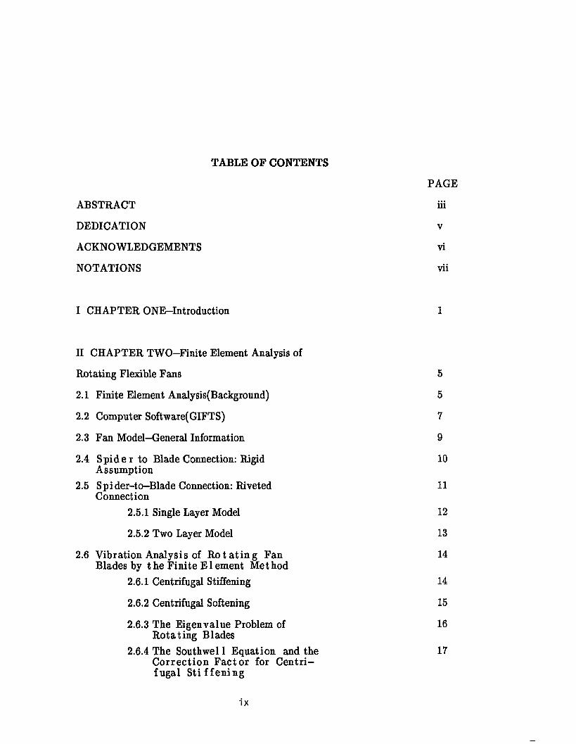
TABLE OF CONTENTS
PAGE
ABSTRACT iii
DEDICATION v
ACKNOWLEDGEMENTS vi
NOTATIONS vii
I CHAPTER ONE—Introduction 1
II CHAPTER TWO—Finite Element Analysis of
Rotating Flexible Fans 5
2.1 Finite Element Analysis(Background) 5
2.2 Computer Software(GIFTS) 7
2.3 Fan Model-General Information 9
2.4 Spide r to Blade Connection: Rigid 10 Assumption
2.5 Spi der-to-Blade Connection: Riveted 11 Connection
2.5.1 Single Layer Model 12
2.5.2 Two Layer Model 13
2.6 Vibration Analysis of R o ta t in g Fan 14 Blades by th e Finite E 1 ement Method
2.6.1 Centrifugal Stiffening 14
2.6.2 Centrifugal Softening 15
2.6.3 The Eigenvalue Problem of 16 R otating Blades
2.6.4 The Southwell Equation and the 17C orrection F ac to r for Centrifugal S tif fe n in g
ix

TABLE OF CONTENTS (continued)
PAGE
2.7 Lim itations on the F in i te Element 19Centrifugal Stiffness Routine
III CHAPTER THREE-Testing 21
3.1 Instrumentation Setup(Static) 22
3.2 Test Procedures(Static) 24
3.3 Instrumentation Setup(Operational) 25
3.4 Test Procedures(Operational) 28
IV CHAPTER FOUR—Discussion of Results 30
4.1 Static Resonance Analysis 30
4.2 The One Blade Model 32
4.3 Operational(Dynamic) Analysis 33
4.3.1 One and Two Layer Model 33
4.3.2 The Southwell Coefficient 33 & C r i t ic a l Speeds
4.3.3 Compar i son of Operat i onal & 34 S t a t i c Tests in the U nitTes t Cage
4.3.4 C om parison fo O p era tio n a l Results 35 in U n it Test C ag e with M odified8 7 . 1 P redic ted Results
x

TABLE OF CONTENTS (continued)
PAGE
V CHAPTER FIVE-Theory and Procedure for the Automatic
Generation of Fan Surfaces for a Dynamic Analysis by
Finite Elements 37
5.1 Introduction 37
5.2 Purpose of the Transformation Program 38
5.3 Theoretical Discussion 39
5.3.1 Straight Camber 39
5.3.2 Camber with Screw 40
5.3.3 Twist in Spider 41
5.3.4 The Generation o f M ulti-B laded 42 Fan Surfaces from One BladeSurface
5.4 P ro c e d u re for F in ite E lem en t Model Gener— 43 a t ion & D eterm ination of Mode Shapesand F req u en ice s
5.4.1 Some Requi r ements for Running 43 th e Program
5.4.2 Taking Measurements 46
5.4.3 Using the Program 46
5.4.4 Using GIFTS to Determine Mode 48 Shapes and Frequencies
VI CHAPTER SIX-Summary 51
6.1 Conlusions 51
6.2 Recommendations 53
xi

TABLE OF CONTENTS (continued)
REFERENCES
APPENDIX 1—F ortran Code for the Transforamtion Program
APPENDIX 2-F igures and Tables for Chapter Two (Figure 2 .1 -2 .6 & Table 2.1-2.3)
APPENDIX 3—Figures for Chapter Three (F igure 3 .1 -3 .1 4 )
APPENDIX 4—Figures and Tables for Chapter Four (F igure 4 .1—4.8 & Table 4.1^4.28)
APPENDIX 5—Figures for Chapter Five (F igure 5.1—5 .7)
APPENIDX 6—Sample Source Files for a One Blade Fan
APPENDIX 7—Files g i v i n g p o i n t s of Rigid Connection i n the Two Layer Model
PAGE
54
58
68
79
94
131
139
148
xii

1
CHAPTER ONE
INTRODUCTION
In 1983 the American Society of Heating, Refrigerating, and
Air-Conditioning Engineers published ASHRAE Standard 87.1—1983, "Method of
Testing Dynamic Characteristics of Propeller Fans — Aerodynamically Excited Fan
Vibrations and Critical Speed" (1). This standard was based on the results of
ASHRAE Research Project RP266, "Propeller Fan Dynamics." (18,19)
Discrepancies have been reported by different users of this standard between critical
speeds predicted by the procedures outlined in the standard for static test data and
critcal speeds that have been obtained in operating tests.
The prediction procedures given in ASHRAE Standard 87.1—1983 did
not adequately take into account the effect of centrifugal stiffening on propeller fan
critical speeds. This is a stiffening that occurs as a result of the centrifugal forces
that act on the distributed mass of the blades of a fan as it rotates. ASHRAE TC
5.1 felt that the discrepancies that have been reported were a consequence of this

2
inadequacy. To correct this, ASHRAE initiated Research Project RP477,
"Development of a Method to Predict Vibration Response of Propeller Fans under
Actual Operating Conditions." The objectives of the project are:
1. Identify and modify, if necessary, a commercially available finite element
program that runs on personal microcomputers and that takes into account
centrifugal stiffening; and
2. Use the program identified in (1) to help explain discrepancies that have
been reported to exist between propeller fan critical speeds predicted in accordance
with ASHRAE Standard 87.1—1983 and the corresponding critical speeds measured
on the same fans in simulated operating conditions.
3. Perform experimental testing on the fans,under static and operating
conditions. The experimental work in this project was done, and Chapter 3 was
written, by Mr. Jeff Bledsoe, under the direction of Dr. Douglas Reynolds and Dr.
William Culbreth. Chapter 3 gives details of the experimental procedures, and it
was included in this thesis, with the permission of its authors, for technical
completeness.
Mainframe-computer based finite element software has long been used
by NASA and other large research institutes for the solution of complex nonlinear
dynamic problems associated with rotating flexible blade structures. Most of these
research activities have focussed on flexible rotating blades related to compressor
and turboprop technology. (7,8,10,11,12,13,15,20,21) Previous efforts that focussed
on fans that are used in heating and refrigeration systems were based on experiment
rather than mathematical modeling.(2,19,20)

3
One of the main disadvantages of using mainframe computer software is
cost. The cost of obtaining and operating mainframe computers and the
corresponding cost of the mainframe software are much higher than the cost of
microcomputers . The microcomputer—based finite element program CASA/GIFTS
was used for the research that is discussed in this report. This powerful program
runs on AT compatible microcomputers and has all the essential capabilities of
mainframe finite element programs. The use of this program on AT compatible
microcomputers brings the cost of using finite element analysis within a range that
can be justified by all major fan manufacturing companies.
The finite element analysis of twisted, flexible and rotating fan blades
that have complex shapes may require considerations and analytical procedures that
are beyond the capability of microcomputer software.(10,ll,13,16,24) This is in
geometrically nonlinear analysis where fans experience large deflections during
normal operating conditions. Restrictions and assumptions associated with the
analysis of rotating fans that experience large deflections can have a direct effect on
the determination of resonance frequencies, mode shapes and related critical speeds.
Factors that should be considered in addition to centrifugal stiffening and
centrifugal softening, include buckling, load updating, and numerical instabilities in
obtaining eigenvalue solutions (4,7,8,10,12,15). In the work reported here,
simplifications were used which are believed to be applicable to most, if not all,
propeller fans used in air conditioning units and heat pumps.
With the cooperation of CASA/GIFTS, finite element models have been
developed that predict propeller fan resonance frequencies and corresponding mode
shapes under rotating as well as non—rotating conditions. (1) In order to account
for the effects of centrifugal stiffening on rotating fans, modifications were made to
the finite element code developed by CASA/GIFTS. GIFTS (6) is a linear finite

4
element program. It does not have the capability to directly deal with nonlinear
problems. The nonlinearities which occur in some of these fans at high rotating
speeds created some difficulties which were overcome with the use of Southwell
coefficients calculated at lower speeds. These coefficients, which were also called the
speed coefficient by Campbell in 1925, have long been used to correlate the
resonance frequencies of blades under non—rotating conditions to the corresponding
resonance frequencies that exist when the blades are rotating. (15,17,25)
A family of five four—blade fans were investigated during this project.
Two fans had flat spiders and were tested only statically to check the initial
development of the finite element models. The other three fans were operational
fans. These fans were tested under simulated operational conditions to determine
the resonance frequencies, mode shapes and corresponding critical speeds associated
with the first-order flapping and twisting modes. These operational test results
were compared with the corresponding results predicted by the current version of
ASHRAE Standard 87.1—1983 and with the corresponding finite element results.

5
CHAPTER TWO
FINITE ELEMENT ANALYSIS OF ROTATING FLEXIBLE FANS
2.1 Finite Element Analysis (Background)
The finite element method is a numerical procedure for solving
continuum mechanics problems with an accuracy acceptable for engineering
practice. The classical method for solving most engineering problems is by partial
differential equations. In practice, many problems are too complicated for a
closed—form mathematical solution. The alternative is a numerical solution, and
finite element analysis is one of the most versatile numerical methods.
Figure 2.1 (in APPENDIX 2) shows a finite element idealization for thin
shallow shell structures such as fan blades. The quadrilateral bending element
shown has four nodes placed at the corners. Each node has the freedom to move in
three orthogonal directions and to rotate about these three orthogonal axes (Figure
2.1a). These translational and rotational movements correspond to the three inplane

6
forces and three moment vectors acting at these nodes midway between the top and
bottom surfaces of the shell. Stresses corresponding to the combined action of the
forces and moments are also ^hown as they act on a shell or plate element. As
shown, a curved shell will have two principal radii of curvature, R1 and R2, and
principal directions, a- and (Figure 2.1b).
Figures 2.2 and 2.3 (in APPENDIX 2) show finite element grids of a one
layer four bladed fan using quadrilateral and triangular elements, respectively. The
elements are connected at the nodes. In modeling fans, either quadrilateral or
triangular bending elements are used. Each node has a total of six degrees of
freedom (three orthogonal translations and three orthogonal rotations). Before the
models in Figures 2.2 and 2.3 were adopted, numerous other models were examined
in this research project. The elements used are individually flat. The curvature of
the blades is approximated by using a sufficiently fine grid of elements.
The trade off in any finite element model is between accuracy and
solution time. The quadrilateral model shown in Figure 2.2 contains 256 elements
with 320 nodes which results in 1848 unknown displacements and rotations in
simultaneous equations. The triangular model in Figure 2.3 contains 560 elements
with 352 nodes resulting in 2040 displacements and rotations. When the finite
element program is run on an AT type microcomputer with a 10 megahertz math
coprocessor, the solution time for computing 8 natural frequencies is 3 hours for the
quadrilateral model and 4 hours for the triangular element model.
Figure 2.4 shows a typical finite element grid of a two layer fan with
triangular bending elements. The fan has a twisted spider and cambered blades with
a full screw. Separate grids are constructed for modeling the twisted spider and the
blades. The two overlaying grids are rigidly connected at discrete points shown by
the big black dots that represent the rivets. This two layer triangular element model

7
contains 584 structural nodes, 928 active elements and a combination of 3288
unknown displacements and rotations in the simultaneous equations. The run time
on an AT type microcomputer for calculating the natural frequencies and mode
shapes is about 13 hours.
The GIFTS program requires that the four nodes of a flat quadrilateral
bending elements must all lie in a plane. Since this may not be the case when
modeling the complex curved surface of a fan blade with a full screw, it is
recommended that triangular bending elements be used for the modeling of fans.
This way a cambered and twisted surface can be represented accurately.
Use of the finite element method is both powerful and potentially
dangerous. Finite elements is a powerful method in that it can be used to solve a
wide range of problems that are otherwise impossible to solve. It is potentially
dangerous in that serious errors, that may be hard to detect by an inexperienced
user, can occur if any of the underlying assumptions or limitations associated with
the finite element program are overlooked by the user.
2.2 Computer Software (GIFTS)
GIFTS, a graphics integrated finite element computer software system,
was used in this research. It can perform static analysis, free and forced vibration
analyses and thermal stress analysis. Free vibration modal analyses of fan
structures is discussed in this report.

8
By computing the vibration modes anJ frequencies of a fan, it is possible
to determine critical rotational speeds that should be given careful consideration in
the design and testing of the fan. The following is a summary of the procedure used
for the modal analysis of fans. First, the geometry of the model was generated by
establishing a series of key points that represent the key features of fan structures.
These key points were then connected by lines or arcs. A grid of elements was
automatically generated by the program from the key points and lines. The hub of
the fan was assumed to be rigidly held. This physical boundary condition of the fan
structure was duplicated in the model by applying constraint conditions to the
various degrees of freedom at the nodes of the model representing the hub.
Determining mode shapes and frequencies required an iterative
eigenvalue-eigenvector solution technique. GIFTS uses a subspace iteration
method for extracting the mode shapes and corresponding resonance frequencies.
Once the mode shapes are obtained, the stresses can be calculated and stress
contours displayed. This can be used to predict potential failure regions in a fan.
The use of models of a single blade was also evaluated. This saves running time it
requires the application of additional constaints at the nodes on the lines which
separate the blade which is modeled horn the blades which are not included in the
model.
The complete command sequence for obtaining a set of mode shapes and
frequencies with GIFTS is given in Section 5.4 .

9
2.3 Fan Model — General Information
The dynamic behaviors of five different four blade fans are presented.
The following is a list describing the five fans tested.
a. Fan with flat spider and flat blades. (CTS4M-025)
b. Fan with flat spider and cambered blades with a radius of curvature of 21
centimeters. (CTS4M-025, std. radius)
c. Fan with twisted spider and cambered blades with no screw. Angle of twist is
32o. (S—17256)
d. Fan with twisted spider and cambered blades with half-screw. (S—17257)
e. Fan with twisted spider and cambered blades with full—screw. (CTS4M
3022-025)
The fans were modeled by first taking accurate measurements of a flat
fan with a flat spider and flat blades. All other models were generated by
mathematical transformations of the geometry of the flat model. For example,
changes were introduced by specifying a twist for the spider, a blade curvature
representing the blade camber, and a prescribed angle of screw and amount of screw
in the blade. The boundary conditions associated with all 4-bladed models were:
(1) the central hole of the spider was inhibited from translation and rotation in all
three directions, and (2) the rest of the structural nodes'had six degrees of freedom.
These nodes were free to translate in three orthogonal directions and rotate about
the three orthogonal axes. In this research, the modeling of the spider—to—blade
connections was treated in a special way. Sections 2.4 and 2.5 give a detailed
explanation of how this connection was modeled. From Figure 3.9 it can be seen
that the four corners of the blades are rounded. In this research, it was determined
that, without loosing accuracy, the top coners need not be rounded, however a
circular curve was included in the model for the lower corners of the blades.

10
2.4 Spider—to-Blade Connection: Kigid Assumption
The fans analyzed in this project have blades which are riveted to the
spider by means of four corner rivets and one central rivet. The first assumption
made in the finite element model was that the spider—to—blade connection was
perfectly rigid and that the thickness of the joint was equal to the combined
thickness of the spider and the blade.
In order to test the accuracy of this model, an experiment was conducted
in which the spider was solidly welded to each blade of a four—blade fan. The two
fans on which this experiment was conducted were: (1) fan with flat spider and
straight camber in the blades, and (2) fan with twisted spider and cambered blades
with a full screw. In modeling the fans with a welded connection, the grids
representing the connection were assumed to be perfectly rigid. The spider and
blade shared the same grids at the connection, and the elements had a thickness
equal to the combined thicknesses of the spider and blade. The properties of the
homogeneous isotropic mild steel were used in the model.
In APPENDIX 2, Table 2.1 shows a comparison between the calculated
and the experimentally measured resonance frequencies of two different fans. The
fans were first tested with the blades riveted and the blades were then welded to the
spider for the second test. The finite element results were calculated assuming a
perfectly rigid connection between the fan blades and spider. As can be seen from
the table, the finite element results did not correlate well with the experimental
results associated with the riveted connection between the fan blades and the spider.
The finite element correlation with the fans in which the fan blades were welded to

11
the spider were much better. This is because the rigid finite element model more
accurately corresponds to the welded connection. These results strongly indicate
that the finite element modeling of the spider—to—blade connection should simulate
the lack of perfect rigidity.
2.5 Spider—to—blade connection: Riveted Connection
The influence of the riveted connection on the effective stiffness of the
fan was examined. A comparison between the finite element and experimental
results indicated that the effective stiffness is influenced by two factors. The first is
the clearance of the rivets and the tightness with which the rivets damp the blade
to the spider. The second is the amount of screw in the blade. The spider is twisted
and usually has a slight straight camber. This yields good surface contact between
it and a blade without a screw. When the blade has a screw plus camber, the
surface contact between the blade and spider is diminished. The overall effective
stiffness between the blade and spider depends on the type of rivet and riveting
techniques used and whether or not the blade is screwed.
Two different approaches were used to model the connection between the
blade and spider. The first used modified material constants in a one layer
orthotropic model. The second used a two layer model.

12
2.5.1 Single Layer Model
A single layer of triangular bending elements was used to represent the
connection between blade and spider for the one layer orthotropic connection.
These elements have a thickness for the connection equal to the combined
thicknesses of the spider and blade. An orthotropic material was used which had
modified shear and Young’s modulii. The values of the shear (G) and Young’s (E)
modulii of the elements representing the connections were modified repeatedly until
the static resonance frequencies of the finite element model were nearly the same as
the corresponding experimental results.
Young’s modulus (E) was obtained by comparing the two nodal line
finite element flapping mode results with the corresponding experimental results.
The shear modulus (G) was obtained by comparing the zero nodal line finite
element twisting mode results with the corresponding experimental results. Several
trial runs were performed to achieve satisfactory results. For the fans examined
during this project, the best results were obtained when the Young’s modulus (E)
equaled 12.5% of the modulus for steel and the shear modulus (G) equaled 27.5% of
the modulus for steel. Table 2.2 shows the effects of material constants G and E on
the fan resonance frequencies.
An advantage of the one layer orthotropic model is that it generates a
smaller number of nodes as compared to the two layer model which is discussed
later. As a result, the runtime is significantly shorter. However, if the riveting
method or blade configuration is changed, a new set of material stiffness constants
must be determined for the new configuration. This can be quite time consuming
and may require several computer runs.

13
2.5.2 Two Layer Model
The two layer model used two separate layers of triangular bending
elements. One layer represented the spider, and the second layer represented the
blade. Point connections between the two layers were introduced to represent the
rivets. The two layers were separated by a distance equal to the length of the rivets.
The two layers were first connected by short beam elements which had the length
and cross-section of a typical rivet. This method yielded resonance frequencies that
closely duplicated the experimental test results. The layers were then assumed to
have rigid point connections in the vicinity of the rivets. The two methods yielded
practically the same results. Since it was the simpler method of the two, the rigid
point connection technique was used for this project.
As discussed earlier, the riveting technique and the degree of screw in
the blade significantly affect the dynamic behavior of a fan. In a like manner, the
positions of the rigidly connected nodes in the two layer finite element model
significantly affected the calculated natural frequencies of the fan. Figure 2.5 shows
the position of the rigidly connected nodes for three different node patterns. The
difference in the positions of the rigidly connected nodes as shown in this figure
accounts for the rivet types and degree of screw in the blades of the fans that were
analyzed during this project. The results shown in element results for two different
fans that had the rigidly connected nodes shown in Figure 2.5 (APPENDIX 2)..
When the rigidly connected nodes are placed farther apart in the radial
direction of the blade, the flapping resonance frequencies increase in value. When
the rigidly connected nodes are placed farther apart in the circumferential direction,
the twisting resonance frequencies increase in value. These characteristics were used
to locate the nodes.

14
It was necessary to employ the "WINDOW" command in the
"LOADBC" processor of GIFTS in order do determine the exact "PN" numbers of
the nodes to be rigidly connected. The two layer model was more exact and gave a
more realistic representation of the riveting method used to connect the fan blades
to the spider. However, this model as compared to the one layer orthotropic model,
had a considerably larger number of unknowns for which to solve. This resulted in a
significant increase (2 to 3 times) in the CPU run. A finite element model for a four
blade fan which uses the two layer technique may require over twelve hours of run
time on an AT microcomputer with a math coprocessor. Even though the one layer
model takes considerably less CPU runtime than the two layer model, the
determination of the equivalent orthotropic material constants for the one layer
model is more time consuming than the positioning of the rigid point connections in
the two layer model. Thus it was decided that the two layer model be used, since it
more closely represented the actual construction of the fans. The exact node
numbers, for rigid connection between the two layers, are shown in APPENDIX 7 in
a series of source files. A step by step procedure of how to use these files is shown in
Section 5.4.
2.6 Vib r atio n Analysis of Botating Fan Blades by the Finite Element Method
2.6.1 Centrifugal Stiffening
When fan blades rotate, centrifugal stresses develop throughout their
structures. These distributed stresses are proportional to the square of the angular
velocity, the distance from the axis of rotation, and the mass density of the blades.
Cantilever fan blades undergo in—plane and transverse displacements and bending

15
and twisting rotations. The centrifugal tensile stresses tend to stiffen the rotating
blades in both the bending and twisting modes. This stiffening increases the natural
frequencies by an amount roughly proportional to the square of the rotation speed.
(15) In the modified version of GIFTS, centrifugal stiffening is taken into account
by setting the total stiffness matrix [K] for the bending of a plate element equal to
the sum of the bending stiffness matrix in the absence of centrifugal forces, [Kb],
plus the centrifugal stiffness matrix [Kc] associated with rotation, or
[K] = [Kb] + [Kc] (2.1)
2.6.2 Centrifugal Softening
In a rotating reference frame, centrifugal stresses have components in the
radial, circumferential, and normal directions of a twisted and screwed blade. A
mass point correspondingly displaces in all three directions. The radially outward
displacement due to the deformation of the blade effectively increases the total
magnitude of the centrifugal force at that point. This is directly proportional to its
radial displacement. This phenomenon contributes to an apparent decrease in the
elastic stiffness of the element, and is called centrifugal softening (11).

16
2.6.3 The Eigenvalue Problem of Rotating Blades
For a rotating plate element, having a setting angle the eigenvalue
problem is expressed as follows: (15)
{[K]— (w2 + a 2sin20) [M]} { d’} = {0} (2.2)
where :
{ d’} = { d } — { d8 } (2.3)
Also a) is the frequency of vibration of the rotating plate, il is the speed of rotation,
[M] is the mass matrix, {d’} is the vector of time dependent component of {d}, {d}
is the vector of nodal displacements for the plate, and {ds} is the vector of time
independent components of {d}.
The eigenvalues and eigenvectors of matrix [K]'1+[M] give the values of
(w2+ n 2sin20) and the mode shapes. In the finite element solution of the twisted and
screwed fan blades, many triangular elements are used to model the blades. The new
version of GIFTS allows for each element to have different setting angles 0 . The
setting angle is defined as the smallest angle at which the plane of each element of
the model is oriented with respect to the plane of rotation.

17
2.6.4 The Southwell Equation and the Correction Factor for C en trifu g a l S tiffen ing
In the ASHRAE 87.1—1983 Standard, the Correction factor for
Centrifugal Stiffening (C), which accounts for the increased bending stiffness due to
the rotation of the fan is approximated by
C = (2.4)- H l/H )2
where H is the harmonic order (H = 1,2,3, ....)
The harmonic H can be determined as follows: H equals the number of blades in a
fan plus or minus the number of nodal lines in a particular mode shape.
This equation for C is the simplified form of a more general equation
given by Yntema (25). C is used to determine the critical speeds, Nc,and N£ is
obtained from
f -60-CN = - 5 ---------- (2.5)
c HNc is the predicted critical speed in RPM.
In the ASHRAE Standard 87.1—1983, C is obtained from equation (2.4)
for the flapping modes and it is assumed to be equal to one for the twisting modes.
During this project, a modified correction factor, C , was obtained for both flappingsand twisting modes. The value of C was obtained using a more accurately
8
calculated value for the Southwell coefficient, S. ,

18
The Southwell coefficient is a constant of proportionality which relates
the squares of the natural frequencies to the square of the rotation speed as follows:
fr2=fn2+S(N/60)2 (2.6)
where fr (Hz) is the resonance frequency associated with the fan rotating at a
specified speed, N (rpm), and f (Hz) is the corresponding resonance frequency for
the case when the fan is not rotating.
When a fan is rotating at a critical speed Nc, the expression for the
resonance frequency at the corresponding mode is
N -Hf = — £----- (2.7)r 60
By eliminating fr from equations (2.6) and (2.7) and substituting equation (2.5) into
the results, an expressio:
coefficient, is derived as
the results, an expression for the correction factor C , which includes the SouthwellO
Cs= 1—(S/H2)(2.8)
The predicted critical speed for any mode is now determined by a modification of
equation (2.5) as follows
f * 60“ CN = - 5 -------- i - (2.9)
c H

19
Equations (2.5) through (2.9) give a more accurate method of predicting the
critical speeds of rotating fans. The determination of the Southwell coefficients and
the corresponding critical speeds for three different four—blade fans will be discussed
in this report.
2.7 Limitations on the Finite Element Centrifugal Stiffness Routine
The previous sections discussed the effect of centrifugal stiffening and
softening on the natural frequencies and critical speeds of rotating fans. For the
flexible fans mentioned in this report, some limitations have to be imposed on the
rotational fan speeds used in the finite element analysis, for the following two
reasons:
(1) Since centrifugal forces are proportional to the square of the angular
velocity, a check on the stresses in the spider and the blades should be made in the
GIFTS processor RESULT before running the processor CSTIFF.
(2) For some fan designs, the center of gravity of the blade may not be in
the plane of rotation. Therefore, the blades will bend under centrifugal forces
towards the plane of rotation. At relatively low speeds the value of this bending
deflection is directly proportional to the square of the rotational speed. Once the
blades have straightened out, however, no further bending can occur. This is a
non-linear phenomenon, which cannot be handled by a linear elastic analysis. If
GIFTS is used at high rotational speeds, unrealistically large normal tip deflections
of the blades are predicted for such fan designs. This leads to a numerical

20
instability, resulting in declining and, ultimately, negative eigenvalues. This
problem is illustrated in Figure 2.6. It is therefore required that a speed of less than
52 radians per second be used to derive the Southwell coefficients (as shown in the
previous section). The southwell coefficients can then be used to calculate the
natural frequencies at higher rotational speeds.

21
CHAPTER THREE
TESTING
Note: The writing of this chapter and the experimentation it refers to was done by
Mr. Jeff Bledsoe under the direction of Dr. William Culhreth and Dr. Douglas
Reynolds. This chapter is included inorder to maintain the technical completeness of
this thesis.
Five propeller fans were tested statically through the use of a test stand
and measurement equipment. The fans that were tested are listed in Section 3.3 of
this report. The guidelines set down in ASHRAE Standard 87.1—1983 were
followed. The specific equipment used in the tests and the testing procedure are
presented in this section.

22
3.1 Instrumentation setup (Static)
The static test system shown in Figure 3.1 used a flat plate of steel with
an approximate mass of 250 lbs and dimensions of 27" x 43" x 5/8". The plate was
welded to vertical steel ribs that considerably stiffened the test assembly. The fans
were attached to a cylindrical piece of steel and tightened down to a minimum
torque of 20 lbf—ft. This setup allowed the different fans to be mounted on the test
stand quickly. The tests that are described in this section were also conducted on
the fans when they were attached to the motor in the test stand used for the
operational tests.
The static tests were performed to determine the resonance frequencies
of each fan and the corresponding modes of vibration. Resonance frequencies were
determined in accordance with ASHRAE Standard 87.1. An accelerometer was
attached to either the leading or trailing tip of a fan blade. A hammer was used to
excite a blade. The piezoelectric accelerometers were chosen for their light weight
and ease of attachment. They had a mass of approximately one gram and were
attached to the fan blade surface with beeswax. This sticky substance allowed good
coupling between the blade surface and the casing of the accelerometer. A
Computer-aided data acquisition system was used to generate the autospectrum
plots associated with each test. This equipment could have been used to determine
the relative phase between two accelerometers, however an oscilloscope was usually
sufficient for this. The instrumentation consisted of two AT compatible Wavepak
cards, a Franklin AT microcomputer, a Hitachi dual trace oscilloscope, and a B&K
function generator.
23
A flowchart for the test setup used for determining the resonance
frequencies is shown in Figure 3.2. This setup consisted of an accelerometer, a signal
amplifier, a hammer and the microcomputer. A photograph showing the setup used
for determining the mode shapes is shown in Figure 3.3, and a flowchart for this
setup is shown in Figure 3.4. This setup consisted of a reference accelerometer, a
roving accelerometer, two signal amplifiers, a function generator, a 100 watt
amplifier, a 4" acoustic speaker, and an oscilloscope. Following is a list of the
equipment used to perform these experiments.
List of Equipment:
1. Franklin AT microcomputer, with 80287 coprocessor
2. Wavepak (Waveform Analysis Package). This consists of two
expansion boards and a software package that allows the
computer to function as a dual—channel FFT signal analyzer.
3. Hitachi dual trace oscilloscope, model # V—650F.
4. Realistic 100 watt solid state P.A. amplifier, model # MPA-90.
5. Piezotronics accelerometers, model # 309A
6. Piezotronics Transducer amplifiers, model # 480d06
7. Piezotronics weighted hammer, model # 086B01
8. Realistic 4" acoustic speaker, model # 40—1022
9. B&k function generator, model # 3010
10. Panasonic dot matrix printer, model # KX—P1091
24
3.2 Test Procedures (Static)
The static tests required that the resonance frequencies be identified and
that the corresponding modes of vibration be determined for the first six modes of
vibration associated with a four blade fan. The experimental procedure required
two parts.
In part one, the resonance frequencies were determined using the test
setup shown in Figures 3.1 and 3.2. A small hammer was used to excite the fan
blades and the autospectrum of the reference accelerometer was observed on the
Franklin AT microcomputer. The Wavepak system computed the autospectrum
through the use of the fast Fourier transform (FFT) and created plots of the
autospectrum that showed the amount of energy per hertz as the ordinate versus the
frequency in Hertz along the abscissa. A typical autospectrum is shown in Figure
3.5 (APPENDIX 3). These tests were performed as specified by ASHRAE Standard
87.1—1983. The accelerometer was mounted on the leading and then on the trailing
tip of each fan blade. All four blades were tapped with the hammer for a total of 32
combinations. The autospectrum was plotted on a dot matrix printer.
In part two, the mode of vibration was determined at each resonance
frequency until the first three flapping and first three twisting modes of vibration
were found. A reference accelerometer was attached with beeswax to the leading tip
of one of the blades and a roving accelerometer was moved freely about the surfaces
of all four blades and the spider. A 4" acoustic speaker was attached to a simple
aluminum assembly that allowed the center of the speaker cone to be placed
approximately 1 inch down and in from the leading edge of the blade where the
reference accelerometer was located. The speaker was placed as close to the blade as

25
possible without interfering with the motion of the fan blad. A sine wave was
provided by a B&K function generator. The generator output was amplified by a
100 watt amplifier and sent on to the speaker. For these tests the first three
flapping and the first three twisting modes were identified, using the autospectrum
plots obtained from the first part. Each frequency was excited with the function
generator and the roving accelerometer was moved around the surface of the fan
blades to determine the mode shape. The outputs from the two accelerometers were
observed on a dual trace oscilloscope to determine the relative phase. After the
determination of the mode shape, the sine wave was then sent to the Franklin AT
microcomputer to provide an accurate determination of the frequency.
3.3 Instrumentation Setup (Operational)
The test stand for this phase of the testing is shown in Figure 3.6. This
special fan cage was provided by the Carrier Corporation. The cage was composed
of a simple support strut assembly located in the center of a perforated steel wall
chamber. The fan motor was mounted on the strut assembly in the vertical
direction. The cage rests on four legs with wheels that allow movement of the cage.
A steel lid attached to the top of the cage protects the operator and bystanders from
debris should a fan failure be encountered. Different fans can be placed on the
motor by lifting the lid of the cage and removing the set screw that attaches the fan
to the fan motor. The cage was designed to allow the fan to blow down towards the
floor. Perforations in the upper lid of the test cage provide minimal and uniform

26
blockage of the air flow. The upper lid was designed to allow for non-uniform
blockage to be added to provide various patterns of non-uniform air flow for blade
excitation.
Variable frequency power was supplied to the fan motor through an
Emerson Industrial Controls Accuspede 270 controller. A remote control box for
the controller that contains the on\off switch, the output voltage, forward and
reverse directions, and the braking current that is provided from the controller was
used. The output of the controller was connected directly to the fan motor in the
test cage. Precautions were made to ground the cage, controller, and transformer
metal coverings to a common point. This was done to eliminate extraneous
electrical noise in the measurement circuitry.
The rotational speeds of the fans were obtained using a simple solar cell,
a frequency counter, and the Wavepak system, which provided an autospectrum of
the solar cell output. The solar cell was contained in a long aluminum tube that
was attached to the bottom of the cage. A flashlight which was attached to the top
of the cage directly above the solar cell was used as a light source to trigger the
solar cell.
Single 120 Ohm strain gauges were affixed to each blade. Strain gauges
were mounted at 45° so that both flapping and twisting modes could be determined
using one strain gauge. All gauges were connected to a terminal strip on the fan
spider through twisted pairs of wire. A slip ring was used to interface the strain
gauges to the strain gauge amplifiers. Shielded cable was used to connect the strain
gauge terminal strip to one side of the Michigan Scientific slip ring. A coupling was
used to mount the slip ring to the shaft of the motor.The center section of the
testing cage lid was removed and the other side of the slip ring was wired to a

27
25—pin connector through two pieces of shielded cable. A copper grounding mesh
was wrapped around the top of the slip ring with wire ties and connected to the
cable ground.
Strain gauge signals were amplified by using a two stage strain gauge
amplifier. This made it possible to amplify the strain signal from 10 to 1000 times.
The amplified signal was passed through a Spectral Dynamics Tracking Filter
(Model No. SD1012B) to remove extraneous noise from the strain signal . The
center frequency of the tracking filter was set equal th the frequency of the strain
signal. The filted Signal was then analyzed using an oscilloscope, and the Wavepak
Spectrum Analyzer was used to determine the frequencies of vibration before the
signal was filtered.
Each fan was tested with the air flow approaching the fan distorted in
the following patterns:
a. a pattern corresponding to the number of blade on fan.
(4 flow interruptions for a 4 bladed fan)
b. A pattern having one more flow retarding sector than the fan
has blades.
(5 flow interruptions for a 4 bladed fan)
c. A pattern having one less sector than the fan has blades.
(3 flow interruptions for a 4 bladed fan)
d. A pattern having two sectors less than the fan has blades.
(2 flow interruptions for a 4 bladed fan)
e. A pattern having two sectors more than the fan has blades.
(6 flow interruptions for a 4 bladed fan)

28
3.4 Test Procedures (Operational Tests)
The Operational tests required that the critical speeds and their
corresponding frequencies and mode shapes be determined. Critical speeds were
determined for the first 6 modes of vibration on the following fans: (1) fan S—17256,
twisted spider and no screw; (2) fan S—17257, twisted spider and half screw; and (3)
fan CTS4M 3022—025, twisted spider and full screw. See Figures 3.8 and 3.9 for
sample photographs of these fans.
To facilitate the tests under operating conditions, a four—channel strain
gauge amplifier was constructed. The strain signals from the four strain gauges on
the four—blade fan were directed through the slip ring to this amplifier. One
channel was selected as a reference. The reference strain signal was directed to the
Wavepak system and to one channel of the two—channel Spectral Dynamics
spectrum analyzer. The signals from the other three strain signals were directed to
a three—position switch. The other three signals, one at a time, were directed to the
second channel of the two-channel Spectral Dynamics spectrum analyzer.
For the operational tests, the frequency at which a specified flapping or
twisting mode occurred was estimated from the procedures outlined in ASHRAE
Standard 87.1—1983. The number of flow obstructions necessary to excite this mode
were placed on top of the test cage. See Figures 3.1 through 3.14 in Appendix 3.
The Wavepak was set on peak-hold to measure and record the maximum strain
signals associated with the reference strain gauge as a function of rotational fan
speed (or frequency). The fan was started at a rotational speed equal to several
hundred rpm below the speed at which the specified vibration mode was expected to
exist. The fan speed was then slowly increased to a speed equal to several hundred

29
rpm above the speed at which the specified vibration mode was expected to exist.
The frequency and corresponding fan speed at which the strain signal was a
maximum were obtained from the Wavepak system.
The center frequency associated with the 5 Hz bandpass filters on the
Spectral Dynamics spectrum analyzer was then set to the frequency obtained from
the Wavepak system.. The signals associated with the reference strain gauge and
one of the other three strain signals were directed through the analyzer to a
two-channel oscilloscope and to a phase meter. The fan rpm was slowly varied over
a small speed range about the center frequency to which the analyzer was set. This
was done until the maximum reference strain signal was obtained. The
three—position switch associated with the other three strain signals was then
switched between the three positions. The corresponding signals were
one—at—a—time compared with the reference signal, noting the phase relationship
between these signals and the reference signal. In this manner, it was possible to
identify the modes associated with their corresponding resonance frequencies. The
precise frequency and corresponding motor rpm at which the the maximum
reference strain occurred was obtained from the Wavepak system.
30
CHAPTER FOUR
DISCUSSION OF RESULTS
4.1 Static Resonance Analysis
The results for the analytical and the experimental work performed on
static fans are summarized in this section. The experimental results were obtained
using the methods obtained in Section 3 of this report. The determination of the
resonance frequencies and corresponding mode shapes was straight forward for all
fans except fan CTS4M 3022-025. This fan had a spider with a 32 degree twist and
blades with a full screw. For this fan it was quite difficult to differentiate between
the different flapping modes. This was attributed to the complexity of the fan
geometry and to the small range of frequencies over which the flapping modes
occurred.

31
The finite element models used to determine the fan resonance
frequencies and mode shapes are described at length in Section 2. The command
sequence and the GIFTS source files are in Appendix B. For these results, two basic
finite element mesh layouts were used, with modifications for the fan geometries as
the only variable in the models. Figures 4.1 through 4.8 show the basic mode shapes
of the four flapping and the four twisting modes. The eight mode shapes are typical
of four—bladed fans.
The first test conducted was on the fan which had a flat spider and a flat
blade. The finite element model for this fan assumed a rigid (instead of riveted)
connection between the spider and the blade. The second test was on the fan which
had flat spider and blades with a straight camber. The numerical and experimental
results of these two fans with simple geometries are shown in Tables 4.1 and 4.2.
The static experimental and finite element results associated with fans
S—17256 (no screw), S—17257 (half screw), CTS4M 3022—025 (full screw) are shown
in Tables 4.3, 4.4 and 4.5. The results in these tables indicate that the finite element
analysis (using a one layer model with modified stiffness constants) compares quite
favorably with the experimental results obtained according to ASHRAE Standard
87.1—1983. Small differences in the frequencies are observed between the fans tested
in the dynamic test cage and on the inertia base according to ASHRAE Standard
87.1. This is due to the influence of the cage and the electric motor on the rigidity
and apparent mass of the fans. Larger differences between corresponding resonance
frequencies are observed with the results obtained by Brookside on different
specimens of the same model fans. This may be explained by possible variations in
the riveting techniques and in the types of rivets used to attach the fan blades to
the spider between the fans tested by Brookside and the fans tested as part of this
project. As was discussed in Section 2, these variations can significantly influence
the natural frequencies of a fan.

32
4.2 The One Blade Model
Either a one—blade or four—blade fan finite element model can be used to
analyze the vibration response of a four—blade fan. The four—blade fan model will
generate all of the desired flapping and twisting modes. The boundary conditions
used for the one—blade model will only generate the non-collective (2—nodal line)
flapping mode and the collective (0—nodal line) twisting mode. Table 4.6 shows a
comparison between the one—blade and four—blade finite element models for the
static case (zero rpm) and for two dynamic cases where the fan rotational velocity
was 20 rad/sec and 52 rad/sec, respectively. The results indicate that the
correlation between the one-blade and four—blade finite element models is very
good. When the one—blade model can be used, a substantial savings in computer
time can be achieved.
33
4.3 Operational (Dynamic) Analysis
4.3.1 One— and Two—Layer Model
The CASA/GIFTS finite element program was modified to incorporate
the effects of centrifugal stiffening. To test the accuracy of this modification and of
the one-layer and two—layer finite element models developed during this project
under simulated operating conditions, finite element analyses were conducted at
specified rotational speeds. The program was run at critical speeds that were
associated with selected resonance frequencies that were measured during
operational fan tests. The resonance frequencies predicted by the finite element
model were then compared to the corresponding measured resonance frequencies. A
comparison of the finite element and corresponding experimental results are shown
in Table 4.7. The results in the table indicate that the correlations between the
one—layer and two—layer finite element results and the corresponding experimental
results were very good. Note that the one layer model had equuivalent material
constants of E equal 0.125 E(steel) and G equals 0.275 G(steel), while the two layer
model had rigid point connection between spider and blade as in Case B of Figure
2.5.
4.3.2 The Southwell Coefficient & Critical Speeds
The mathematical procedure for calculating the Southwell coefficients for
the four—blade fans that were investigated during this project was discussed in
Section 2.6.4. Two fan models were examined: (1) one blade and (2) four blades.
The Southwell coefficients were obtained using two different rotational speeds: (1)
20 rad/sec and (2) 52 rad/sec. For each fan that was examined and for each of the
two models, two finite element runs were made: (1) at zero rpm (static case) and

34
(2) at one of the two specified rpm’s (dynamic case). The respective Southwell
coefficients were calculated using equation (6) and the correction coefficients
corresponding to each Southwell coefficient and related harmonic order was obtained
from equation (8). Tables 4.8 through 4.10 give the results for the three fans tested
for the one-blade model operating at 0 and 20 rad/sec. Tables 4.11 through 4.13
give the results for the four—blade model operating at 0 and 52 rad/sec. Tables 4.14
through 4.16 give the results for the one—blade model operating at 0 and 20 rad/sec.
Tables 4.17 through 4.19 give the results for the four—blade model operating at 0
and 52 rad/sec.
Comparisons between the one- and four-blade results and between the
results associated with rotational speeds of 20 rad/sec and 52 rad/sec indicate that
the variations in the respective Southwell coefficients were fairly small. Since the
speed correction factor Cs in equation (9) is related to the Southwell coefficient by a
square root operation, the variations in the corresponding correction factors were
even smaller. Thus, with respect to the fans that were investigated during this
project, any angular velocity between 20 rad/sec and 52 rad/sec can be used to
calculate the Southwell coefficients and either a 4—bladed model or a 1—bladed
model can be used with nearly equal accuracy.
4.3.3 Comparison of Operat i onal Resul ts in Unit Test Cage with S t a t i c Tests in the Unit T est Cage
Tables 4.20 through 4.22 show a comparison between the measured
critical speeds for the three fans tested during operational tests and the
corresponding results predicted by the procedures outlined in ASHRAE Standard
87.1—1983. This comparison indicates that the predicted values deviated by as

35
much as 17% to 23% from the measured values. Typical deviations of 4% to 10%
were common. It is these high deviations that were to be reduced by the project
discussed in this report.
For these comparisons, the static test results obtained with the fan
mounted on the motor in the unit test cage were used rather than the test results
obtained in accordance with ASHRAE Standard 87.1—1983. The reason for this is
that the purpose of the comparison is to evaluate the effect of centrifugal stiffening
by itself. For this purpose, it is better to use static test results taken under
conditions which differ from those of the dynamic test results only by the absence of
rotation. If the comparison were made against static test results obtained in
accordance with ASHRAE standard 87.1—1983, it would be necessary to account for
the installation effects discussed in Appendix B of ASHRAE Standard 87.1—1983.
4.3.4 Comparison of Operational Results in Unit Test Cage with Modif ied 87.1 Predicted Resul ts
Tables 4.23 through 4.28 show a comparison between measured critical
speeds for the three fans tested during operational tests and the corresponding
results predicted by the proposed modified ASHRAE Standard 87.1 procedures.
The Southwell coefficients and corresponding speed correction factors that were used
in these tables are the same as those that have been previously discussed. This
comparison indicates that the maximum deviations between predicted and measured
results were reduced from 17% to 23% down to 7% to 14%. Typical deviations
ranged from 2% to 5%. This is a substantial improvement relative to the current
ASHRAE Standard 87.1—1983 procedures.

36
Nearly all of the cases where the deviation between predicted and
measured results exceeded 7% are associated with the one—nodal line flapping and
twisting modes. The one nodal line flapping and twisting modes can occur in
several different possible combinations on a four—blade fan. This can possibly
account for the consistently large discrepancies that occurred with these modes.
It should be noted that the 87.1—1983 procedure for predicting critical
speeds was based on the assumption that the Southwell coefficient was S=1.0 for the
flapping modes and S=0 for the twisting modes. This project has shown that these
assumed values are not adequate and that much more accurate predictions can be
made by using Southwell coeffiecients calculated by the finite element method.
Tables 4.23 through 4.28 also show that it is quite adequate to use a finite element
model of a single blade with proper boundary conditions applied to the nodes shared
with those blades which are not included in the model.

37
CHAPTER FIVE
THEORY AND PROCEDURE FOR THE AUTOMATIC GENERATION
OF FAN SURFACES FOR A DYNAMIC ANALYSIS
BY FINITE ELEMENTS
5.1 Introduction
This chapter contains mathematical transformation analyis, a fortran
code and manual. A fortran program is presented which facilitates the procedure of
analyzing the dynamic, behaviour of fan blades under static or operating conditions,
by the Finite Element Method. The first section of the chapter shows the
derivations of the mathematical transformations, which create surfaces representing
a number of cylindrically curved and warped blades along with their associated
twisted spider. The blades and spider surfaces are generated from one flat shaped
blade and one associated sector of the spider. The second section gives a step by

38
step procedural input guide to the fortran program, which in turn generates
complete input data files to be used by the finite element program GIFTS in
predicting the mode shapes and frequencies of fan blades under actual operating
conditions .
5.2 Mathematical Transformations Analysis
5.2.1 Purpose of the Mathematical Transformation Program
When modeling any structure by using the finite element method, an
accurate set of measurements should be taken of the structure in question in order
to create the best fitting finite element mesh which represents it. Most fan blades
have a complicated geometry, and the task of measuring the key points representing
the topographical outline of the blades in 3—D, could be very difficult, time
consuming, and error prone. On the other hand, measurements taken on a fan with
a flat sider and blade is simpler and more accurate. The analysis presented uses the
measured coordinates of number of specified key points on one flat blade and its
associated sector of a flat spider, and creates a curved, screwed and twisted set of
blades by performing the following transformations when requested: 1. To put a
camber, a screw or both in the blade. 2. to twist the spider. 3. to generate a number
of fan blades by repeated coordinate transformations. Results of the analysis are
interpreted by a fortran program which generates an output file, formatted as a
source file, which in turn is used by the finite element code GIFTS in predicting the
mode shapes and frequencies of fan blades under actual operating conditions..

39
5.3 Theoretical Discussion
The next four sections give a discussion of the theory involved in the
transformations. The program performs these operations in the order they appear in
this text.
5.3.1 Straight Camber
The explanation and equations in this section refer to Figure(5.1). In this
figure R is the radius of curvature of the blade and S’ is the arclength Rom the
center of the blade to its edge. The original cartesian coordinates of the blade are
centered at the hub or axis of rotation, with the y axis being along the length of the
blade, the x axis along the width of the blade, and the z axis being the axis of
rotation. The local coordinates on the flat spider and blade are defined as Xj, y^and
zj, and the transformed coordinates are defined as x i} and zt. The following
equations refer to Figure(5.1) and show how the transformation is performed:
(5.1)R
where S = x i (x coordinate of flat blade)
Xj = R • sin 9 (5.2)
z, = R • [1—cos 3 ] (5.3)
The computer program includes these transformations in Subroutine CAMBER.

40
5.3.2 Camber with Screw
The transformation that introduces the warp or screw in the blade is
based on the follwoing assumption (refering to Figure(5.2)): Any point along the
line ( n ) will have the same z coordinate. Line ( n ) goes through point O at an
angle of <J> from the y axis, where (j) is the angle of screw in the blade. Since point O
is attached to the spider then its z coordinate will be equal to zero, and based on the
mentioned assumption we can say that the z coordinate of any point along line ( n )
will be equal to zero when the spider is flat. The ardength associated with any other
point on the blade after camber will be equal to the perpendicular distance between
that point and line(n) when the blade is flat. We are also assuming that the
principal radius of curvature R is constant in the blade and the surface generated is
a skewed cylinder. The equation defining line ( n ) is as follows:
y = - tan(90 — <J>) • x + yQ (5.4)
where the slope is [—tan(<J> + 90)], and the y intercept is yQ
The arclength S’ associated with any point i is defined as follows:
g>= tan(9<H>)-;, + y (6 5)
i [tan(9(H>)! + l 2]1/ 2

41
Referring to Figure(5.3), we can see that the angle 6 is defined as in
equation (5.1). Figure (5.3) shows the position of the transformed coordinates with
respect to the original coordinates and the following equations give the relationships
between the local and transformed coordinates:
x. = x. — [S’— R*sin(0)]-cos(<|>)
y = y — [S’- R-sin(0)]-sin(<|>)
z. = R -[l—cos(0)]
The computer program includes these transformations in Subroutine SCREW.
5.3.3 Twist in Spider
The transformation for a twist in the spider is performed in the x,z plane
only, and the relation between the original and transformed coordinates is as
follows:
x. = x.-cos(^) + z.-sin(^)
y. = y.1 1
z. = x.*[-sin(^)] + z.-cos (ip)
where ip is the angle of twist in the spider
The computer program includes these transformations in Subroutine TWIST.
(5.9)
(5.10)
(5.11)
(5.6)
(5.7)
(5.8)

5.3.4 The Generation of a Multi—Bladed Fan Surface from One B lade Surface
Once the coordinates of one flat blade have been transformed to create a
cambered, screwed and twisted surface, succesive transformations are performed to
generate the respective coordinates of other blades in the fan. The blade generating
transformationa are performed in the x,y plane. The angle of transformation is in
increments of 360 divided by the number of blades. The equations of transformation
are as follows:
x. = x.*cos(^i ) + y.*sin(^ ) (5.12)
(5.13)
(5.14)
y. = x.-[-sin(^» )) + y *cos(ip )
z = zz = z i iwhere ip =
n 360 j and (k = l,n)
The computer program includes these transformations the Subroutine BLADES.

43
5.4 Procedure For Finite Element Model Generation and Determination of Mode Shapes and Frequencies
5.4.1 Some Requirements for Running the Programs
The following sections give a step by step procedure of how to use the
transformation program and how to integrate it with the finite element software
package,GIFTS. All the files needed are in the diskette accompanying this report.
The list shown below gives the requirements for generating a Finite Element Model
for Propeller fans.
(A) GIFTS should be installed on the hard disk of a PC/AT microcomputer, as
mentioned in the GIFTS Release Notice Accompanying the software.
(B) It is also advisable to read at least the following chapters in the GIFTS
PRIMER MANUAL: ch.l(General Remarks), ch.7(The RESULT Postprocesing
Program), ch.9(Determination of Natural Modes of Vibration). Another helpful step
is to follow the procedure in one of the EXAMPLE PROBLEMS in the GIFTS
PRIMER MANUAL. Note that the most useful example for our fan problem is
EXAMPLE 6 entitled "PLATE".

(C) Check if the following files are in the accompanying diskette. The contents of
these files can be verified by comparison with the explanation given bellow.
1. TRANSF.EXE 2. CENTSTIF.BAT
3. IMPUT.DAT 4. OUTPUT.DAT
5. 1LIMPUT.DAT 6. 2LIMPUT.DAT
7. 1L2BIN.DAT 8. 2L2BIN.DAT
9-20. FANB1L1.SRC, FANB1L2, FANB2L1,...FANB6L2 (To ta l o f 12 f i le s )
21-26. BC1.SRC, BC2.SRC, BC4.SRC, BC5.SRC, BC6.SRC
27-44. PRIGB1A . SRC, PRIGB1B.SRC....PRIGB6C.SRC (T o t al o f 18 f il e s)
1. TRANSF.EXE : This an execution file of the program which performs the
transformations.
2. CENTRIF.BAT : This is a batch file that can be used to find mode shapes and
frequencies under centrifugal stiffening.
3. IMPUT.DAT : This file contains the imput data that is read in by the
transformation program. The format of this imput file is shown in a later section.
4. OUTPUT.DAT : This is the output file of the transformation program, and it
contains all the key points necessary for creating a fan model using GIFTS.
5. 1LIMPUT.DAT : This is a sample input file for a one layer model of a fan with
1,3,4,5 or 6 blades. Kepoint numbering for this model is shown in Figure(5.4). Note
that this file and the next three files need to be copied on to IMPUT.DAT once they
are prepared, because TRANSF.EXE only reads from file IMPUT.DAT.

45
6. 2LIMPUT.DAT : This is a sample input file for a two layer model of a fan with
1,3,4,5 or 6 blades. Keypoint numbering of a two layer model is shown in
Figure(5.5). Note in the file that the z coordinates of the spider nodes are at z
equals zero, while the z coordinates of the blade nodes are at z equals 1.0
centimeters. The two layers are connected by the PRIGCON command at desired
nodes.
7. 1L2BIN.DAT : This is a sample input file for a one layer mode of a fan with 2
blades. The key node numbering is shown in Figure(5.6).
8. 2L2B1N.DAT : This is a sample input file for a two layer model of a fan with 2
blades. The key node numbering is shown in Figure(5.7).
9-20. FANB1L1.SRC, FANB1L2.SRC, FANB2Ll.SRC...FANB6L2.SRC(Total of
12 files): These source files contain the lines and grids that connect the keypoints
generated by the program. In each one of these files, the number after the letter B
stands for the number of blades in the fan(l—6), and the number after the letter L
represents the number of layers used in the model,(one layer or two layers).
21-26. BC1.SRC,BC2.SRC,BC3.SRC,BC4.SRC,BC5.SRC,BC6.SRC : These source
files contain the commands for applying boundary conditions and generating the
mass matrix, for fans with 1,2,3,4,5 and 6 blades respectively.
27-44. PRIGB1A.SRC,PRIGB1B.SRC,PRIGB1C.SRC,...PRIGB6C.SRC: These
files give the rigidly connected nodes in the two layer model of the fans. The number
after the letter B denotes the number of blades in the fan(l-6), and the last letter in
the filename (before .SRC) refers to cases A,B or C as shown in Figure 2.5
(APPENDIX 2). Case A is used for welded spider—to—blade connections. Case B is
used for fans with twisted spider and blades with half or no screw, having a riveted
connection. Case C is for fans with twisted spider and blades with a full screw,
having a riveted connection.

46
5.4.2 Taking Measurements
The first step in generating a Finite Element model is to take accurate
measurement of the fan. Figures(5.4,5.5,5.6,and 5.7) show the key node numbering
systems used by the program for a flat fan. First make a trace of one blade of the
flat fan, and mark the node numbers as shown in the respective figure. Measure the
coordinates of each node with respect to the center of the hub. Note that in
Figures(5.4 & 5.5) nodes 101 and 103 are colinear with the origin, and these nodes
are at an angle } v ipn from y axis. In Figures (5.4 & 5.5), nodes 201 and 203 need to
be inputed for a run with a one blade fan,and need not be defined for fans with more
than one blade because the program will automatically generate these nodes.
5.4.3 Using the Transformation Program
First copy all the files in the accompanying diskette in the GIFTS
directory.The next step in using the transformation program is to create an input
file. The input file should have the following format:
K,K1,K2,R,ASC,AT,NBL,YBLD
KPN1
W i
KPN2
x 2>y2>Z2
KPNi
xi.yi.zi

47
The input file should be in the same format and order shown above. The
variables are defined as follows:
K = TOTAL NUMBER OF KEY POINTS IN ONE BLADE.
K1 = ORDER NUMBER OF TH E FIRST NODE TO BE INCLUDED IN THE TW IST TRANSFORMATION
K2 = ORDER NUMBER OF THE FIR ST NODE TO BE INCLUDED IN THE SCREW OR CAMBER TRANSFORMATION
R = RADIUS OF CURVATURE OF THE BLADE.
ASC = ANGLE OF SCREW IN THE BLADE IN DEGREES.
AT = ANGLE OF TWIST IN THE BLADE IN DEGREES.
NBL = TOTAL NUMBER OF BLADES IN THE FAN.
YBLD =Y COORDINATE OF THE BOTTOM/CENTER NODE OF THE BLADE W H ICH CORRESPONDS TO NODE # 1 0 9 IN FIG U R E ( 5 . 4 ) .
KPNi = KEY POINT NUMBER i.
x* = x COORDINATE OF KEY POINT # i.
y* = y COORDINATE OF KEY POINT # i.
zj = z COORDINATE OF KEY POINT # i.
Once the input file is saved and checked, the transformation program should be
executed using the following commands:
C> COPY Filename.DAT IMPUT.DAT (example: 1LIMPUT.DAT)
C> TRANSF
When the program execution is complete, then check the output file and copy it into
a source file as follows:
O C O P Y OUTPUT.DAT Filename.SRC (example: PNTB1L1.SRC)

48
The file (Filename. SRC) will contain all the key point necessary for creating the
model. At present we have a source file that is acceptable to GIFTS, and we are
ready to create the model and determine mode shapes and frequencies of the fan.
Note that a convenient way of naming Filename.SRC would for example
PNTB4L1.SRC, where the numbers after the letters B and L represent the number
of blades in the fan and layers in the model respectively.
5.4.4 U sing GIFTS to Determine Mode Shapes and Frequencies Under S t a t i c C onditions o r C entrifugal Forces
The following are set of GIFTS commands used in order to determine
mode shapes and frequencies.
C>BULKM (Generates the model)TYPE JOBNAME:.....
*OLB ( N o t e that o n l y t h e fi 1 enam e is used) > . . ( e n t e r source f i 1 ename c o n t a i ning keypoints)
(PNTB1L1 or PNTB2L2 o r PNTB4L1 . . . ect .*OLB> . . . . ( e n t e r SRC f i l e contain i n g grids & lines)
(FANB1L1 or FANB2L2 or FANB4L1 ... ect.)*PLOT
*QUIT
C>LOADBC ( Apply boundary conditions & centrifugal forces) TYPE JOBNAM E:......
*OLB> . . . ( e n t e r SRC f i l e containg boundary conditons)
(BC1 OR BC2 0 R BC3 ...ECT )*ANGVEL,3 > ................ ( enter angular velocity in rad/sec)
(om it this command if there are no centr i fugal f orces involved)

49
*OLB> . . . (enter SRC fi le con t a i n i ng p o i n t s o f r igid
connection, example: PRIGB6C OR PRIGB1A)♦PLOT
♦QUIT
C>
At this point there are two different sets of commands to be followed
depending on wether centrifugal forces are applied or not. The following are two
complete lists of commands (including the above) for performing a dynamic analysis
with or without centrifugal forces.
A. Command Sequence for Dymanic Analysis under Static Conditions(Nonrotating)
1) BULKM :generate the model
2) LOADBC :apply boundary conditions
3) BULKF :suppre s s unwantedfreedoms
4) OPTIM :optimize the bandwith
5) Macro STIFF : compute and assemble the stiffnessm at r ix
6) SUBS :compute natural frequencies
Note: Steps 3 to 5 can be repalced by a batch file MMODES.BAT.

50
B. Command Sequence for Dynamic Analysis including Centrifugal St i f fening (Rotating F a n s )
1) BULKM :generate the model
2) LOADBC :apply boundary conditions andcentrifugal forces
3) BULKF :suppress unwanted degree of freedom
4)^OPTIM (see note below) :optimize the bandwith *
5) Macro Stiff : compute and assemble the stiffnessm at r ix
6) SAVEK :save the stiffness matrix
7) DECOM :decompose the stiffness matrix
8) DEFL :compute the deflections
9) STRESS :compute the stresses $
10) CSTIFF :compute the stiffness due to initialst r esses
(* Note that commands 5 to 10 can be substituted with the
batch file CENTSTIF.BAT. This is achieved with the following
command: C>CENTSTIFF,Jobname)
11) SUBS :compute natural frequencies
Once the natural frequencies are detemined and the mode shapes are
extracted then all the information can be found in the processor RESULT.
"*’Note:When GIFTS returns with the request/'enter wavefront #1", use
the following node numbers, which give the shortest solution time:
>124
>126

51
CHAPTER SIX
SUMMARY
6.1 Conclusions
1. The GIFTS finite element program modified by the CASA/GIFTS
Corporation to take into account the effects of centrifugal stiffening, was found to be
adequate for the purposes of this project.
2. With respect to the range of operational parameters that were
investigated during this project, the finite element results predicted by GIFTS
correlated very well with corresponding measured static and operational fan
vibration results.
3. Depending on the information desired, either a one—blade or four blade
finite element analysis can be used to investigate the vibration characteristics of a
four—blade fan.
4. The rivets that are used to attach the fan blades to the spider and the
tightness of the rivets significantly influence the values of the resonane frequencies
associated with the twisting modes of a fan.

52
5. The finite element analysis yielded vibration results that correlated well
with operational test results over the entire range of fan operating speeds which
were possible with the test unit (1600 — 1800 rpm). The Southwell coefficients
calculated with the finite element program permit predictions of critical speeds as
high as 2,800 rpm, but it was not possible to obtain operational test data at this
speed.
6. Finite element analyses can be used to calculate Southwell Coefficients
that relate the resonance frequencies that exist at zero rpm to the corresponding
resonance frequencies that exist at specified rotational speeds. Southwell
coefficients calculated for rotational speeds between 20 and 52 rad/sec were found to
be suitable for the purposes of this project. Even though it is possible to calculate
Southwell coefficients at higher rotational speeds this tends to cause problems due
to the linear nature of the speeds finite element analyses used.
7. Critical speeds can be predicted with acceptable accuracy using
Southwell coefficients calculated using either a one— or four—blade fan model for a
four—blade fan and using assumed operational speeds of either 20 rad/sec or 52
rad/sec.
8. Using Southwell coefficients that were calculated by means of the finite
element models developed during this investigation, the accuracy of the fan critical
speed prediction procedure outlined in ASHRAE Standard 87.1—1983 was
substantially improved with respect to the four-blade fans that were tested.
Maximum deviations between ASHRAE predicted and experimentally measured
test results were reduced from 17% to 23% down to 7% to 14%. Typical deviations
were reduced from 4% to 10% down to 2% to 5%. The accuracy of the prediction
procedure was improved by a factor of two.

53
6.2 Recommendations
1. Only a four—blade fan with a rather simple spider and blade geometry
was examined during this investigation. This investigation should be expanded to
fans with more complicated spider and fan geometries to ensure that the procedures
developed during this investigation accurately apply to these situations.
2. Three—, four— five— and six—blade fans are commonly used in HVAC
systems. Three—, five— and six—blade fans should be examined to ensure that the
procedures developed during this investigation accurately apply to these fans.
3. The typical accuracy of the procedures developed during this project
varied between 2% and 5% for the fans that were examined. If greater accuracy is
desired, it will be necessary to develop more complicated and lengthier (such as
nonlinear and/or iterative) finite element procedures to accomplish this.
4. For greater accuracy, the interaction between the vibrational modes of
the fan and the mass/elastic properties of the drive motor and its support in the
unit would have to be taken into account.

54
REFERENCES
1. ASHRAE Standard 87.1—1983, "Method of Testing Dynamic—
Characteristics of Propeller Fans — Aerodynamically Excited Fan Vibrations and
Critical Speeds".
2. Baade, P.K., "Measurement Techniques for Preventing Fan Vibration
Failure," Proceedings of Machinery Vibration Monitoring and Analysis Seminar,
Vibration Institute, Clarendon Hills, IL, pp.27—36,1979.
3. Beckwith, Thomas G.; Lewis, Buck N.; Marangoni, Roy D., Mechanical
Measurements," Reading Mass.: Addison—Wesley Publishing Co., 1982.
4. Co, C.J., "Coriolis Effects on the Vibrations of Rotating Beams, Plates
and Shells," Ph-D Dissertaion, Ohio State University, 1984.
5. Cook, R.B., "Concepts and Applications of Finite Element Analysis,"
2nd Edition, Wiley, New York, 1981.
6. GIFTS, "Computer Aided Structural Analysis Graphical Interactive
Finite Element Total System," CASA/GIFTS Inc., Nov. 1985.
7. Kielb, R.E.; Leissa, A.W.; MacBain, J.C.; and Carney, K.S.: Joint
Research Effort on Vibrations of Twisted Plates, Phase I: Final Results, NASA
Reference Publication 1150, Sept. 1985.
8. Kielb, R.E.; Leissa, A.W.; and MacBain, J.C.: Vibration of Twisted

55
Cantilever P lates- A Comparison of Theoretical Results. International Journal of
Numerical Methods in Engineering, Vol.21, Issue 8, August 1985, pp.1365—1380.
9. Ladkany, S.G., et. al., "Dynamic Finite Element Analysis of Fan
Blades," Progress Report ASHRAE Project # 477—RP, Civil and Mechanical
Engineering Department, University of Nevada, Las Vegas, March 1987.
10. Lawrence, C., Kielb, R.E.: "Nonlinear Displacement Analysis of
Advanced Propeller Structures using NASTRAN," NASA TM—83737,1984.
11. Lawrence, C., et al.: "A NASTRAN Primer for the Analysis of Rotating
Flexible Blades," NASA TM—89861, May 1987.
12. MacBain, J.C.; Kielb, R.E.; and Leissa, A.W.: "Vibrations of Twisted
Cantilever Plates—Experimental Investigation," ASME Paper 84—GT-S6, 1984.
13. McGee, O.G., "Finite Element Analysis of Flexible Rotating Blades,
"NASA TM-89906, July 1987.
14. Oden, J.T., "Finite Element Applications in Non-Linear Structural
Analysis," Proc. Symp. on Applications of Finite Element Methods in Civil
Engineering, Am. Soc. Civ. Eng., Vanderbilt Univ., 1969.
15. Ratwani, S., and Dokainish, M.A., "Vibration Analysis of Rotating
Cantilever Plates, "International Journal for Numerical Methods in Engineering,"
Vol. 3, 233-248,1971.
16. Ratwani, S., and Dokainish, M.A., "Bending of Pretwisted Cantilever
Plates," Trans. Can. Aeronaut. Space Inst., Vol. 2, 89-94,1969.
17. Ratwani, S., and Dokainish, M.A., :Vibration Analysis of Pretwisted
Cantilever Plates," Trans. Can. Aeronaut. Space Inst., Vol. 2, 95—100,1969.
18. Reynolds, D.D., and Carnes T.N., "Propeller Fan Dynamics, I. Static
Vibration Test Procedure, and II. Dynamic Vibration Test Procedure," to be
published in ASHRAE Trans.
19. Reynolds, D.D., "Test Procedures for Static and Dynamic Vibration

56
Testing of Propeller Fans, Final Project Report," ASHRAE Project No. 266, June
29, 1981.
20. Sreenivasamurthy, S., and Ramamurti, V., "A Parametric Study of
Vibration of Rotating Pre-twisted and Tapered Low Aspect Ratio Cantilever
Plates," J. Sound Vibr., Vol. 76, June 8, 1981, pp.311—328.
21. Srinivasan, A.V., and Fulton, G.B., "Advanced Turboprop Vibratory
Characteristics," (R84—956627—1, United Technologist Research Center; NASA
Contract NAS3-23533) NASA CR-174708, 1984.
22. Timoshenko, S.P., and Gere, J.M., "Theory of Elastic Stability,"
McGraw-Hill, 2nd edition, 1961.
23. "Wavepak User’s Manual," Computational Systems, Inc., Knoxville,
Tennessee, March 1986.
24. Yeh, C.H., "Large Deflection Dynamic Analysis of Thin Shells Using the
Finite Element Method," Ph.D. Thesis, University of California, Berkeley, 1970.
25. Yntema, R.T., "Simplified Procedures and Charts for the Rapid
Estimation of Bending Frequencies of Rotating Beams," NASA Technical Note
3459, June 1955.
26. Zienkiewicz, O.C., "The Finite Element Method," 3rd edition,
McGraw-Hill, (UK), 1977.

57

APPENDIX 1
FORTRAN CODE FOR THE TRANSFORMATION PROGRAM

59
C
cC MAIN PROGRAM
C
C THIS PROGRAM PERFORMS THE FOLLOWING FUNCTIONS:
C 1. OPENS THE INPUT AND OUTPUT FILES.
C 2. READS ALL THE PARAMETERS NEEDED TO PERFORM THE
TRANSFORMATIONS
C 3. CALLS THE NECESSARY SUBROUTINES FOR THE
TRANSFORMATIONS.
C
IMPLICIT DOUBLE PRECISION(A-H,0-Z)
COMMON/ONE/K,K1,K2)R,ASC,AT,NBL,YBLD,KPN(200)
COMMON/TWO/X(200),Y(200),Z(200)
COMMON/THREE/XSC(200),YSC(200),ZSC(200)
COMMON/FOUR/XT(200),YT(200),ZT(200)
COMMON/FIVE/XBL(600,8),YBL(600,8),ZBL(600,8),KPNF(600,8)
OPEN(UNIT=3,FILE=,C:\GIFTS\IMPUT.DAT,,STATUS=’OLD’)
OPEN(UNIT=4,FILE=’C:\GIFTS\OUTPUT.DAT’,STATUS=’NEW’)
C
DO 25 1=1,200
X(I)=0
Y(I)=0
Z(I)=0
25 CONTINUE

60
C AT = ANGLE OF TWIST IN DEGREES ,
C ASC= ANGLE OF SCREW IN DEGREESC
C R= RADIUS OF CURVATURE
C K = TOTAL # OF KEY POINTS IN ONE BLADE
C K1 = NUMBER OF FIRST NODE TO BE INCLUDED IN THE TWIST
TRANSFORMATION
C K2 = NUMBER OF FIRST NODE TO BE INCLUDED IN THE CAMBER OR
SCREW TRANSFORMATION.
C NBL = TOTAL NUMBER OF BLADES ON THE FAN.
C YBLD= Y COORDINATE OF BOTTOM/CENTER NODE OF THE BLADE
C
C
C THE FOLLOWING SET OF COMMANDS READ THE DATA FROM A FILE
IMPUT.DAT
C
READ(3,*)K,K1,K2,R,ASC,AT,NBL,YBLD
DO 10 1=1, K
READ(3,*)KPN(I)
READ(3,*)X(I),Y(I),Z(I)
10 CONTINUE
C
C

61
C THE FOLLOWING SET OF COMMANDS CALL THE NECESSARY
SUBROUTINES.
C
ASC=ASC/57.29578
IF(ABS(ASC).LT.0.02)THEN
CALL CAMBER
ELSE
CALL SCREW
ENDIF
CALL TWIST
CALL BLADES
CALL SRCFILE
CLOSE(3)
CLOSE(4)
STOP
END
C

62
C CAMBER PROGRAM
C
C THIS SUBROUTINE PERFORMS THE TRANSFORMATION FOR A
CAMBERED BLADE WITH NO SCREW, OR IF THE ANGLE OF SCREW IS
LESS THAN TEN DEGREES.
C
SUBROUTINE CAMBER
IMPLICIT DOUBLE PRECISION(A-H.O-Z)
COMMON/ONE/K,K1,K2,R,ASC,AT,NBL,YBLD,KPN(200)
COMMON/TWO/X(200),Y(200),Z(200)
COMMON/THREE/XSC(200),YSC(200),ZSC(200)
DO 50 I=K2,K
S=X(I)
THETA= S/R
X(I)=R*SIN (THETA)
Z(I)=R*(1—COS(THETA))
Y(I)=Y(I)
KPN(I)=KPN(I)
50 CONTINUE
RETURN
END
C

63
C SCREW PROGRAM
C
C THIS PROGRAM PERFORMS THE SUBROUTINE FOR A SCREW OR
WARP IN THE BLADE.
SUBROUTINE SCREW
IMPLICIT DOUBLE PRECISION(A-H,0-Z)
COMMON/ONE/K,K1,K2,R,ASC,AT,NBL,YBLD,KPN(200)
COMMON/TWO/X(200),Y(200),Z(200)
COMMON/THREE/XSC(200),YSC(200),ZSC(200)
DO 60 I=K2,K
S=((—TAN(ASC—1.570796)*X(I))+Y(I)—YBLD)/SQRT((—TAN(1.570796—ASC
1 ))**2+l)
THETA=S/R
PRJ=R*(SIN (THETA))
DELTA=S-PRJ
ASCR=ASC
X(I)=X(I)—(DELTA*COS(ASCR))
Y(I)=Y(I)-(DELTA*SIN(ASCR))
Z(I)=R*(1—COS(THETA))
KPN(I)=KPN(I)
60 CONTINUE
RETURN
END

64
C TWIST PROGRAM
C
C THIS PROGRAM PERFORM THE TWIST IN THE X,Z PLANE
C
C
SUBROUTINE TWIST
IMPLICIT DOUBLE PRECISION(A-H,0-Z)
COMMON/ONE/K,K1,K2,R,ASC,AT,NBL,YBLD,KPN(200)
COMMON/TWO/X(200),Y(200),Z(200)
COMMON/THREE/XSC(200),YSC(200),ZSC(200)
COMMON/FOUR/XT(200),YT(200),ZT(200)
AT=AT/57.29578
DO 40 I=K1,K
X(I)=(X(I)*COS(AT))-(Z(I)*SIN(AT))
Z(I)=(X(I)*SIN(AT))+(Z(I)*COS(AT))
Y(I)=Y(I)
KPN(I)=KPN(I)
40 CONTINUE
RETURN
END

65
C BLADES PROGRAM
C THIS PROGRAM PERFORMS THE TRANSFORMATION IN THE X,Y
PLANE IN ORDER TO ACCOUNT FOR THE NUMBER OF BLADES IN THE
FANS.
SUBROUTINE BLADES
IMPLICIT DOUBLE PRECISION(A-H,0-Z)
COMMON/ONE/K,K1,K2,R,ASC,AT,NBL,YBLD,KPN(200)
COMMON/TWO/X(200),Y(200),Z(200)
COMMON/FOUR/XT(200),YT(200),ZT(200)
COMMON/FIVE/XBL(600,8),YBL(600,8),ZBL(600,8),KPNF(600,8)
M=0
DO 70 J=1,NBL
DO 80 1=1,K
P J= J-1
THETA=(2*3.141592654/NBL)*PJ
XBL(I,J)=(X(I)*COS(THETA))—(Y(I)*SIN(THETA))
YBL(I,J)=(X(I)*SIN(THETA))+(Y(I)*COS(THETA))
ZBL(I,J)=Z(I)
KPNF(I,J)=KPN(I)+M
80 CONTINUE
M=M+100
70 CONTINUE
RETURN
END

66
C SOURCE FILE PROGRAM
c t h i s S u b r o u t i n e w r i t e s t h e o u t p u t in a f o r m a t t h a t
C IS ACCEPTABLE BY GIFTS.
C
SUBROUTINE SRCFILE
IMPLICIT DOUBLE PRECISION(A-H,0-Z)
COMMON/ONE/K,K1,K2,R,ASC,AT,NBL,YBLD,KPN(200)
COMMON/FIVE/XBL(600,8),YBL(600,8),ZBL(600,8),KPNF(600,8)
WRITE(4,*),KPOINT’
DO 90 J=1,NBL
DO 100 1=1, K
WRITE(4,200)KPNF(I,J)
WRITE(4,300)XBL(I,J),YBL(I,J),ZBL(I,J)
100 CONTINUE
90 CONTINUE
200 FORMAT(2X,I4)
300 F0RMAT(1X,E12.5,1X,E12.5,1X,E12.5)
RETURN
END

67

APPENDIX 2
FIGURES AND TABLES FOR CHAPTER TWO

69
Figure 2.1 a. Finite Element idealization of the nodal displacements of a thin and
shallow shell structure.
-♦ = Translation Displacements
-+-* = Rotation Displacements
-7
(3)

70
Figure 2.1 b. Stresses, principal radii of curvature R^ and Rg, and principal
directions and in acurved shell element.

71
Figure 2.2 Typical Finite Element grid with quadrilateral elements.

Figure 2.3 Typiacl Finte Element grid with triangular elements.

73
Figure 2.4 Typical Finite Element Grid of a fan using two layers of triangular
bending elements in the overlap area of the spider with the blade.

Figure 2.5 Finite Element grid showing points if rigid connection between the two
layers of triangular bending elements.
Case A. Used for welded or braized connection.
Case B. Used for fans with twisted spider & blades with half or no screw; riveted connection.
\/VN/N\/ 4 / l \ i Z , \ . / l
r x -'16\v /T X I/.
\ l / l \ *
Case C. Used for fan with twisted spider & blades with a full screw; riveted connection.

Nat
ural
Fr
eque
ncy
(Hi)
N
atur
al
Fre
qu
en
cy
!^
75
Figure 2.6 Illustration of the limitation of the Linear Analysis for calculating
Centrifugal Stiffness of a fan with a twisted spider and full screw.
Flapping Mode
SO “
4 0 -
,J3 a
30 -
20 -
10 -
Q 4 0 BO 200 240
Angular V daaty{rad/see)D U r e a ’ A n d y o p *1* E x trapo la tion
Twisting Mode120
1 1 0 -
100 -
9 0 "
00 -' ' ( I
7 0 -
00200 240BO0 4 0
Angubr Velocity ( ra n /se c )□ Unesa- atovbb 1* E x trapolation

76
Table 2.1 Comparison of resonance frequencies between riveted and welded
spider—to—blade connection.
Fan CTS4M-025 -- Fan with flat spider and camberedblades.
Mode of Resonance FrequenciesVibration ------------------------
RIVETED WELDED RIGIDCONNECTION CONNECTION CONNECTIONExperimental Experimental F.E. Model
Flapping,2 nodal line 29.87Twisting, ---------collective 47.10
Fan CTS4M 3022-025 — Fan with twisted spider & blades with a full screw
Flapping,2nodal line 25.60 28.49 27.10Twisting, -----------------------------------------collective 51.10 66.25 66.43
29.6860.38
33.00 62 .50

77
Table 2.2 Fan frequencies due to variations in the effective stiffness parameters of
the spider—to-blade connection.
Fan CTS4M-025 — Fan with flat spider and cambered bladesFREQUENCIES (Hz)
Computed by Finite Elements ExperimentalEffective YoungsModulus(% of E) 60 % 40 % 20 % 12.5 %Effective ShearModulus(% of G) 19 % 21 % 20 % 27.5 %MODE 1 31.77 31.31 30.27 29.54 29.88MODE 2/3 Flapping 32.72 32.23 31.12 30.31 30.03MODE 4 34.58 34.01 32.71 31.76 32.27MODE 5 45.44 45.92 45.44 47. 38 45.50MODE 6/7 Twisting 46.11 46.60 46.09 48.08 46.55MODE 8 46.44 46.93 46.04 48.44 47.16
Fan S-17256 — Fan with twisted spider and cambered blades(no screw)FREQUENCIES(Hz)
Computed by Finite Elements ExperimentalEffective YoungsModulus(% of E) 30 % 15 % 20 % 12.5 %Effective ShearModulus(% of G) 30 % 30 % 20 % 27.5 %Mode 1 32.28 31.10 31.44 30.64 30.43Mode 2/3 Flapping 32.46 31.24 31.64 30.78 30.26Mode 4 34 .50 32.97 33.49 32.41 31.78Mode 5 '49.96 49.41 46.20 48.52 48.42Mode 6/7 Twisting 50.16 49.61 46.36 48.71 49.43Mode 8 50.91 50.34 46.97 49.41 50.33

78
Table 2.3 Fan frequencies of the two layer model due to variation in position of
rigid point connection between blade and spider. (Postioning of Cases A,B, and C
are shown in Figure 2.5).
MODE SHAPE RESONANCE FREQUENCIESCase A Case B Case C Experimental
S-1726 — This fan has and a spider with a 32
four blades, a straight camber, degree pitch.
Flapping, 2nodal lines 32.83 32.13 30.26 30.43Twisting, 0nodal lines 56.17 48.67 38.60 50.33
CTS4M 3022-025 --- This fan has four blades with a fullscrew and a spider with a 32 degree pitch.Flapping, 2nodal lines 27.09 26.20 25.12 25.91Twisting, 0nodal lines 66.44 62.29 54.59 51.06

APPENDIX 3
FIGURES AND TABLES FOR CHAPTER THREE

Figure 3.1 Photograph of system used for determining resonance frequencies.

Figure 3.2 Instrumentation setup for determining resonance frequencies.
Ttjp i « a I F a n
Mb AT
Con f a i n s U « v « ' . k A/D C . i » < • o J F F T i * f i n s a *

Figure 3.3 Photograph of system used for determining modes shapes.
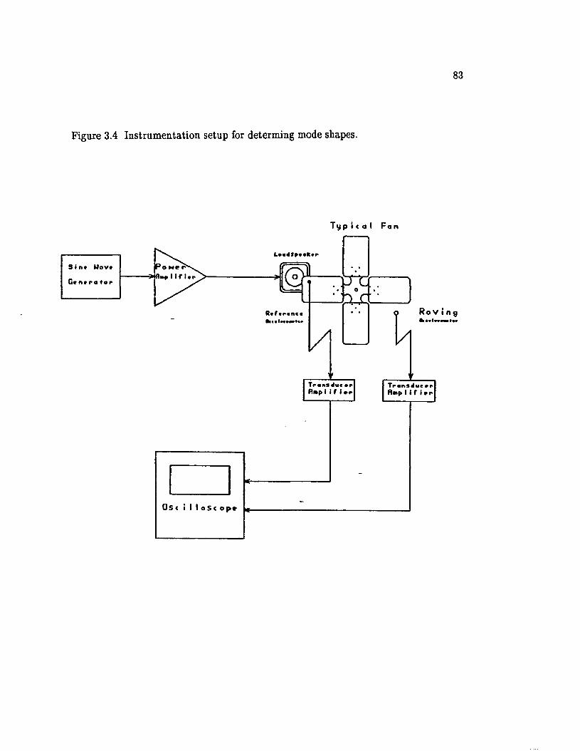
83
Figure 3.4 Instrumentation setup for determing mode shapes.
T y p i c a l F a n
S i n * H av*
Ro V i n•n.inrai
R t f i n n c t
T r r f v c mr T r c n s d v e »r» R n p I I f I » r
3

84
P e a
Figure 3.5 Typical Autospectrum of a four blade fan.
AVGR SPEC- CHAHMEL-X DB <REF :i. 0000013)10 RMSincocu
- 1 0
cr*•
C DCO
fljuo-3 G cua* o'* in ■
- 4 0
20 4 0 6 0FREQUENCY IN HZ
P e a k L i s t f o r C h a n n e l - X S p e c t r u m
.k n um b e r F r e q u e n c y P e a k V a l u e( H= ) dB ( 1 . 0 0 0 0 0 0 )
1 2 S . 5 4 S - 1 7 . 4 5 32 2 0 . 2 4 0 - 3 5 . 2 5 43 4 7 . S 5 0 - 1 3 . 7 2 2

85
Figure 3.6 Photograph of test stand for dynamic testing.

86
Figure 3.7 Instrumentation setup for operational tests.
R n o I o g
F r a n k I i n AT Ml« •■pMt»P
U a V t p a k f i /D C o n v a n d F F T s o f t n a r t

87
Figure 3.8 Photograph of fan CTS4M-025.

88
Figure 3.9 Photograph of fan CTS4M-025 (std. rad.).

89
Figure 3.10 Two flow interruptions. Corresponds to a harmonic order of 2 and 2
nodal lines.

Figure 3.11 Three flow interruptions. Corresponds to a harmonic order of 3 and 1
nodal line.

91
Figure 3.12 Four flow interruptions. Corresponds to a harmonic order of 4 and the
collective modes.

92
Figure 3.13 Five flow interruptions. Corresponds to a harmonic order of 5 and 1
nodal line.

93
Figure 3.14 Six flow interruptions. Corresponds to a harmonic order of 6 and 2
nodal lines.

APPENDIX 4
FIGURES AND TABLES FOR CHAPTER FOUR

1
..h o n o d a l^ es-
M odel,

96
Figure 4.2 Mode 2, flapping mode with 1 nodal line.

97
de 2 but abift64 90 ' Mode3,5am ea8ia

98
Yigviie 4.4Mo d e 4 ,c o U e c * v e ^
mode.

Figure 4.5 Mode 5, twisting mode with 2 nodal lines.

Figure 4.6 Mode 6, twisting mode with 1 nodal line.

101
Figure 4.7 Mode 7, same as mode 6 but shifted 90°

Figure 4.8 Mode 8, collective twisting mode.

CD CT
\ U1
U W
H
103
Table 4.1 CTS4M—025 This fan had four flat blades with no pitch and no camber.
FrequencyExperimental
Flapping ModesMode Nodal Lines
2 1 2 . 0 01 1 1 . 9 21 1 1 . 9 20 1 3 . 1 3
Twisting ModesNodal Lines
2 33.251 38.961 33.960 39.25
Analytical Relative % error
1 2 . 8 91 2 . 9 41 2 . 9 4 1 3 . 0 3
7 . 48.68.60 . 7
3 6 . 6 63 6 . 9 03 6 . 9 0 3 7 . 0 4
4 . 25 . 35 . 3 5 . 6

104
Table 4.2 CTS4M-025 (Standard radius) This fan had four blades with a straight
camber, and a spider with no pitch.
Mode Nodal Lines FrequencyExperimental Analytical Relative % error
Flapping Modes2110
29. 88 30.0330. 03 32.27
29.543 0 . 3 13 0 . 3 331.76
1.11.01.01 . 6
wisting Modes2110
4 5 . 5 04 6 . 6 4 4 6 . 6 4 4 7 . 1 6
4 7 . 3 8 4 8 . 0 8 4 8 . 0 9 4 8 . 4 4
0 . 43 . 13 . 1 2 . 7

Table 4.3 Fan S—17256 (no screw).
Table showing resonance frequencies and the correspondingnode specification for fan S-17256 (twisted spider, caiber, no screw)
ResonanceResonance Frequencies
Node of Nuiber of Obtained byVibration Nodal Lines Brookside
Frequencies Resonance Obtained withFrequencies Fan in DynaaicObtained by 87.1 Test Cage
Flapping 2 36.5 30.43 30.30Flapping 1 37.2 30.26 27.50Flapping 0 38.3 31.78 33.20Twisting 2 51.7 48.42 47.90Twisting 1 52.0 49.43 48.82Twisting 0 54.1 50.33 49.79
Resonance Frequencies Obtained by Finite Eleient Method, Single Layer Model
30.64
30.87
32.4148.5248.81
49.91

Table 4.4 Fan S—17257 (half screw).
Table showing resonance frequencies and the corresponding ■ode specification for fan S-17257 (twisted spider, caiber, 1/2 screw)
ResonanceFrequencies
Mode of Nuiber of Obtained byVibration Nodal Lines Brookside
ResonanceFrequencies
Resonance Frequencies Obtained with Fan in Dynamic
Obtained by 87.1 Test CageFlapping 2 29.5 29.04 28.93Flapping 1 28.8 28.64 26.02Flapping 0 30.8 30.94 31.50Twisting 2 59.3 50.66 50.32Twisting 1 60.0 49.83 50.43Twisting 0 62.7 52.53 52.55
Resonance Frequencies Obtained by Finite Eleaent Method, Single Layer Model
29.9930.11
31.4650.0750.3551.22
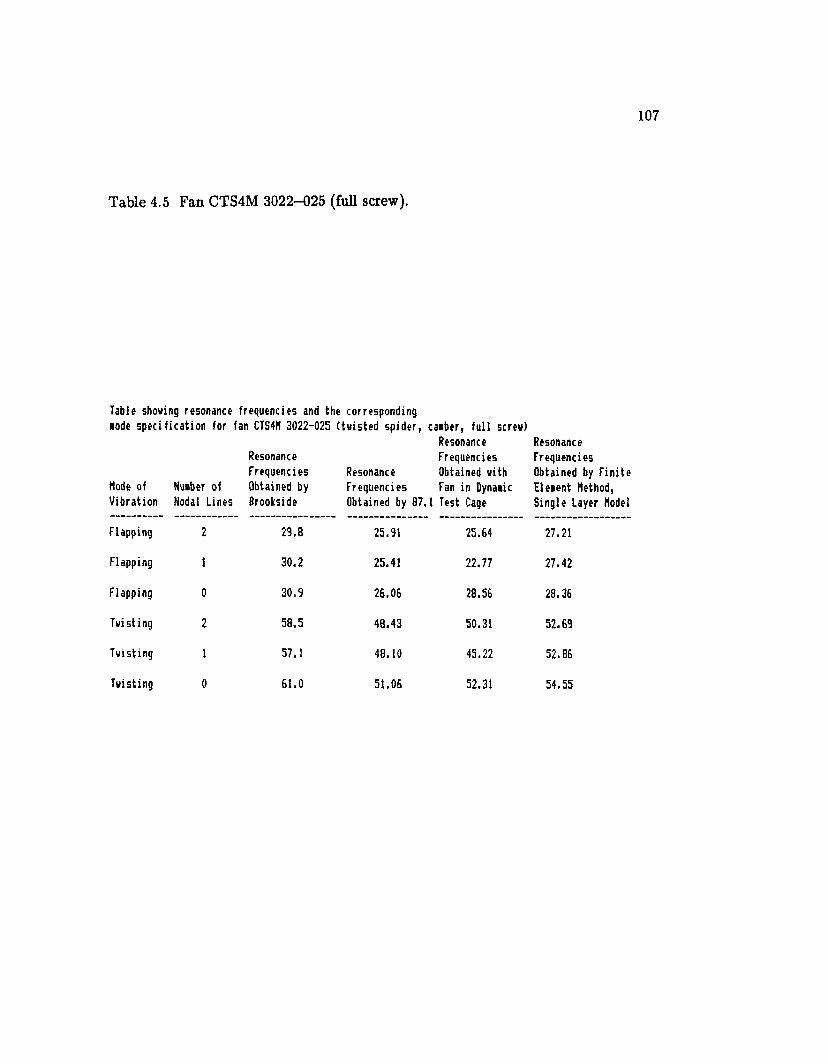
107
Table 4.5 Fan CTS4M 3022-025 (full screw).
Table shoving resonance frequencies and the corresponding■ode specification for fan CTS4H 3022-025 (twisted spider, caaber, full screw)
Resonance Frequencies
Resonance Obtained withFrequencies Fan in DynaaicObtained by 87.1 Test Cage
ResonanceFrequencies
llode of Nuaber of Obtained byVibration Nodal Lines 8rookside
Resonance Frequencies Obtained by Finite Eleaent Method, Single Layer Model
Flapping 2 29.8 25.91 25.64 27.21Flapping 1 30.2 25.41 22.77 27.42Flapping 0 30.9 26.06 28.56 28.36Twisting 2 58.5 48.43 50.31 52.69Twisting t 57.1 48.10 45.22 52.86Twisting 0 61.0 51.06 52.31 54.55

108
Table 4.6 Table comparing resonance frequencies obtained by finite element
analysis using 1 and 4 bladed models.
Mode Shapes Resonance FrequenciesStatic Run (0 rad/sec)
Dynamic (20 rad/sec)
Runs(52 rad/sec)
1 blade.4 blades - 1 blade.4 blades - 1 blade.4 bladesS-17256 — Fan with NO SCREW.
with twisted spider and cambered blades
Flapping, 2. nodal lines.
32.13 _ 31.72 _ 32.32 _ 31.92 _ 33.38 _ 32.99
Twisting, 0. nodal lines.
48.69 _ 48.89 _ 48.88 _ 49.08 49.95 50.12
S-17257 — Fan with twisted with a HALF SCREW.
spider and cambered bladed
Flapping, 2. nodal lines.
30.58 _ 30.14 _ 30.79 _ 30.36 _ 31.97 _ 31.56
Twisting, 0. nodal lines.
52.81 _ 52.83 _ 53.04 _ 53.05 54 . 31 54.28
CTS4M 3022-025 — Fan with ' blades with FULL SCREW.
twisted spider and cambered
Flapping, 2. nodal lines.
25.71 _ 25.12 _ 26.01 _ 25.44 _ 27.58 27.07
Twisting, 0. nodal lines.
54.45 _ 54.60 _ 54.72 _ 54.86 _ 56.20 56.26

109
Table 4.7 Computed vs. measured dynamic frequencies at various critical speeds.
S-17256— This is a ONE LAYER MODEL of a fan having four blades, a straight camber, and a spider with a 32 degree pitch. This model uses equivalent material constants for the spider/blade connection of E=.125 E(steel) & G=.275 G(steel).
Mode Harmonic Shape Order
F.E.StaticFrequency(Hz)
MeasuredCriticalSpeed(RPM)
F.E.DynamicFrequency(Hz)
MeasuredDynamicFrequency(Hz)
Flapping,2 . nodal lines.
2 30. 64 975 35.46 33.60
Flapping,0 . nodal lines.
4 32.41 497 34.55 34 . 65
Twisting,2 . nodal lines.
6 48.52 496 50.28 49.75
Twisting, 1 . nodal line .
3 48.80 980 53.14 51.63
Twisting, 0 . nodal lines.
4 49.94 764 52.93 51.00
S-17256— This is a TWO LAYER MODEL of a fan having four blades, a straight camber, and a spider with a 32 degree pitch. The rigid point connection between spider and blade is identical to Case B of Figure 2.5.
Mode Harmonic Shape Order
F.E.StaticFrequency(Hz)
MeasuredCriticalSpeed(RPM)
F.E.DynamicFrequency(Hz)
MeasuredDynamicFrequency(Hz)
Flapping,2 . nodal lines.
2 31.72 975 35.71 33 . 60
Flapping,0 . nodal lines.
4 33 .78 497 34.99 34.65
Twisting,2 . nodal lines.
6 47.62 496 48.90 49.75
Twisting,1 . nodal line .
3 47.85 980 52.35 51.63
Twisting,0 . nodal lines.
4 48.89 764 51.58 51.00

Table 4.8 Fan S—17256 (no screw), 1 bladed model, 20 rad/sec.
Finite Eleaent ResultsFan 5-17256, caabered blades without screw, twisted spider Rotating Speed 20 rad/sec = 3.18 Hz1 bladed aodelFlapping fo FE
N calc.H f (stat.) f (rot) S Cs (rpa)
2 Nodal Lines
26
32.1332.13
32.3232.32
1.211.21
1.201.02
1154327
1 Nodal Line
35
0.000.00
1.001.00
Collect.Flapping
4 0.00 1.00
TwistingH f (stat.) f (rot) s Cs
fo FE N calc,
(rpa)2 Nodal Lines
26
0.000.00
1.001.00
1 Nodal Line
35
0.000.00
1.001.00
Collect.Twisting
4 48.69 48.87 1.73 1.06 773

Table 4.9 Fan S-17257 (1/2 screw), 1 bladed model, 20 rad/sec.
Fan S-17257, half screw, twisted spiderFinite Eleaent ResultsRotating Speed 20 rad/sec =1 bladed aodel
3.18 Hz
FlappingH f (stat.) f (rot) S Cs
fo FE N calc,
(rpa)
2 Nodal Lines
26
30.5830.58
30.7830.78
1.211.21
1.201.02
1099311
1 Nodal Line
35
0.000.00
1.001.00
Collect.Flapping
4 0.00 1.00
TwistingH f (stat.) f (rot) S Cs
fo FE N calc,
(rpa)2 Nodal Lines
26
0.000.00
1.001.00
1 Nodal Line
35
0.000.00
1.00 1.00
C o llec t . 4 52.81 53.03 2.30 1.08 856Twisting

Table 4.10 Fan CTS4M 3022-025 (full screw), 1 bladed model, 20 rad/s.
Fan CTS4H 3022-025, full screw, twisted spider Finite Ele»ent ResultsRotating Speed 1 bladed aodel
20 rad/sec 3.18 Hz
Flapping
H f (stat.) f (rot) S Cs
fo FE N calc,
(rpi)
2 Nodal Lines
2S
25.7125.71
26.0126.01
1.531.53
1.271.02
982263
1 Nodal Line
35
0.000.00
1.001.00
Collect.Flapping
4 0.00 1.00
TwistingH f (stat.) f (rot) S Cs
fo FE N calc,
(rpi)
2 Nodal Lines
26
0.000.00
1.001.00
1 Nodal 3 0.00 1.00Line 5 0.00 1.00Collect. 4 54.45 54.72 2.91 1.11 903Twisting

113
Table 4.11 Fan S—17256 (no screw), 4 bladed model, 20 rad/sec.
Finite Eleaent ResultsFan S-1725B, caabered blades without screw, twisted spiderRotating Speed 4 bladed aodel
20 rad/sec 3.18 Hz
Flapping fo FE N calc.
H f (stat.) f (rot) S Cs (rpa)
2 Nodal 2 31.72 31.91 1.19 1.19 1136Lines 6 31.72 31.91 1.18 1.02 3231 Nodal 3 32.22 32.40 1.15 1.07 690Line 5 32.22 32.40 1.15 1.02 396Collect. 4 33.78 33.96 1.20 1.04 527Flapping
Twisting fo FE N calc.
H f (stat.) f (rot) S Cs (rpa)
2 Nodal 2 47.62 47.81 1.81 1.35 1930Lines 6 47.62 47.81 1.81 1.03 4891 Nodal 3 47.87 48.06 1.80 1.12 1070Line 5 47.87 48.06 1.80 1.04 596
C o l le c t . 4 48.89 49.08 1.84 1.06 779Twisting

Table 4.12 Fan S-17257 (1/2 screw), 4 bladed model, 20 rad/sec.
Fan S-17257, half screw, twisted spider Finite Eleaent ResultsRotating Speed 4 bladed aodel
20 rad/sec 3.18 Hz
FlappingH f (stat.) f (rot) S Cs
fo FE N calc,
(rpa)
2 Nodal Lines
26
30.1430.14
30.3630.36
1.311.31
1.221.02
1103307
1 Nodal Line
35
30.5530.55
30.7530.75
1.211.21
1.071.03
657376
Collect.Flapping
4 31.86 32.06 1.26 1.04 498
TwistingH f (stat.) f (rot) S Cs
fo FE N calc,
(rpa)2 Nodal Lines
26
51.8951.89
52.1252.12
2.362.36
1.561.03
2432537
1 Nodal 3 52.20 52.45 2.58 1.18 1236Line 5 52.20 52.45 2.58 1.06 661C o l le c t . 4 52.82 53.05 2 .40 1.08 859Twisting

Table 4.13 Fan CTS4M 3022—025 (full screw), 4 bladed model, 20 rad/s.
Fan CTS4N 3022-025, full screw, twisted spider Finite Eleaent ResultsRotating Speed 20 rad/sec = 3.18 Hz4 bladed aodel
Flapping fo FEN calc.
H f (stat.) f (rot) S Cs (rpa)2 Nodal Lines
26
25.1225.12
25.4325.43
1.551.55
1.281.02
962257
1 Nodal Line
35
25.5025.50
25.8225.82
1.621.62
1.101.03
563316
Collect.Flapping
4 26.34 26.65 1.62 1.05 417
Twisting
H f (stat.) f (rot) S Csfo FE
N calc, (rpa)
2 Nodal Lines
26
53.0553.05
53.3053.30
2.622.62
1.711.04
2714551
1 Nodal Line
35
53.5453.54
53.7853.78
2.542.54
1.181.06
1264678
Collect.Twisting
4 54.60 54.85 2.70 1.10 898

Table 4.14 Fan S—17256 (no screw), 1 bladed model, 52 rad/s.
Finite Eleaent ResultsFan 5-17256, caabered blades without screw, twisted spiderRotating Speed 1 bladed aodel
52 rad/sec 8.28 Hz
Flapping
H f (stat.) f (rot) S
fo FE N calc.
Cs (rpa)
2 Nodal Lines
26
32.1332.13
33.3833.38
1.201.20
1.191.02
1151327
1 Nodal Line
35
0.000.00
1.001.00
Collect.Flapping
4 0.00 1.00
TwistingH f (stat.) f (rot) S
NCs
fo FE calc, (rpa)
2 Nodal Lines
26
0.000.00
1.001.00
1 Nodal Line
35
0.000.00
1.001.00
Collect. 4 48.69 49.95 1.81 1.06 776Twisting

117
Table 4.15 Fan S—17257 (1/2 screw), 1 bladed model, 52 rad/s.
Fan S-17257, half screw, twisted spider Finite Eleient ResultsRotating Speed 1 bladed aodel
52 rad/sec 8.28 Hz
Flapping
H f (stat.) f (rot) SN
Csfo FE calc, (rpa)
2 Nodal Lines
26
30.5830.58
31.9731.97
1.271.27
1.211.02
1110311
1 Nodal Line
35
0.000.00
1.00 1.00
Collect.Flapping
4 0.00 1.00
TwistingH f (stat.) f (rot) s
NCs
fo FE calc, (rpa)
2 Nodal Lines
26
0.000.00
1.001.00
1 Nodal Line
35
0.000.00
1.001.00
Collect.Twisting
4 52.81 54.31 2.35 1.08 858
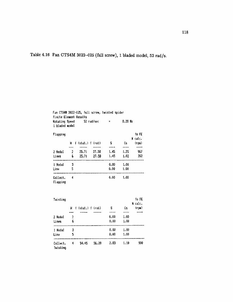
118
Table 4.16 Fan CTS4M 3022—025 (full screw), 1 bladed model, 52 rad/s.
Fan CTS4M 3022-025, full screw, twisted spider Finite Eleient ResultsRotating Speed 1 bladed aodel
52 rad/sec 8.28 Hz
Flapping
H f (stat.) f (rot) S Cs
fo FE N calc,
(rpa)
2 Nodal Lines
26
25.7125.71
27.5827.58
1.451.45
1.251.02
967262
1 Nodal Line
35
0.000.00
1.001.00
Collect.Flapping
4 0.00 1.00
TwistingH f (stat.) f (rot) S Cs
fo FE N calc,
(rpa)
2 Nodal Lines
06
0.000.00
1.001.00
1 Nodal 3 0.00 1.00Line 5 0.00 1.00
Collect. 4 54.45 56.20 2.83 1.10 900Twisting

Table 4.17 Fan S—117256 (no screw), 4 bladed model, 52 rad/s.
Finite Eleaent ResultsFan S-17256, caobered blades without screw, twisted spiderRotating Speed 4 bladed aodel
52 rad/sec=
8.28 Hz
FlappingH f (stat.) f (rot) S
fo FE N calc.
Cs (rpa)
2 Nodal Lines
26
31.7231.72
32.9932.99
1.201.20
1.201.02
1137323
1 Nodal Line
35
32.2232.22
33.4533.45
1.181.18
1.071.02
691396
Collect.Flapping
4 33.70 34.99 1.29 1.04 527
TwistingH f (stat.) f (rot) S
fo FE N calc.
Cs (rpa)2 Nodal Lines
26
47.6247.62
48.8648.86
1.751.75
1.331.03
1904488
1 Nodal Line
35
47.8747.87
49.1349.13
1.781.78
1.121.04
1069596
Collect.Twisting
4 48.89 50.12 1.78 1.06 778

Table 4.18 Fan S—17257 (1/2 screw), 4 bladed model, 52 rad/s.
Fan S-17257, half screw, twisted spider Finite Eleaent ResultsRotating Speed 52 rad/sec = 9.28 Hz4 bladed lodelFlapping fo FE
N calc.
2 Nodal Lines
H f26
(stat.)30.1430.14
f (rot)31.5631.56
S1.281.28
Cs1.211.02
(rpi)1096307
1 Nodal 3 30.55 31.95 1.28 1.08 660Line 5 30.55 31.95 1.28 1.03 376
Collect.Flapping
4 31.86 33.24 1.31 1.04 499
Twisting fo FEN calc.
H f (stat.) f (rot) S Cs (rpi)2 Nodal 2 51.89 53.33 2.21 1.50 2328Lines 6 51. B9 53.33 2.21 1.03 C/1 CO O'!
1 Nodal 3 52.20 53.69 2.30 1.16 1210Line 5 52.20 53.69 2.30 1.05 657Collect. 4 52.82 54.28 2.28 1.08 856Twist ing

121
Table 4.19 Fan CTS4M 3022-025 (full screw), 4 bladed model, 52 rad/s.
Fan CTS4M 3022-025, full screw, twisted spider Finite Eleaent ResultsRotating Speed 52 rad/sec = 8.28 Hr4 bladed aodel
Flapping fo FEN calc.
H f (stat.) f (rot) S Cs (rpa)2 Nodal 2 25.12 27.07 1.49 1.26 951Lines 8 25.12 27.07 1.49 1.02 2571 Nodal 3 25.50 27.45 1.51 1.10 559Line 5 25.50 27.45 1.51 1.03 316
Collect. 4 26.34 28.26 1.53 1.05 415Flapping
TwistingH f (stat.) f (rot) S Cs
fo FE N calc,
(rpa)
2 Nodal Lines
26
53.0553.05
54.7054.70
2.602.60
1.691.04
2686551
1 Nodal Line
35
53.5453.54
55.2455.24
2.702.70
1.201.06
1280680
Collect.Twisting
4 54.60 56.26 2.69 1.10 898

122
Table 4.20 Fan S-17256 (no screw), Experimental values.
Fan 3-17256 Resonance In Unit Dynanic Test ResultsFrequencies CalculatedObtained with Critical Speeds Resonance Critical I dev.
Hod* of Number of Fan in Dynanic H a r s o m c Based On 87.1 Frequency Speeds fromVibration Nodal Lines Test Cage Order Results in Unit (Hz) (RPM) ■easured
0i . 1141 33.60 333 14.3
Flapping 2 30.13 —6 336 30.30 303 10.303 620 28.70 570 8.3
Flapping 1 26.31 —
5 358 30.85 370 -3.1Flapping 0 33.20 4 517 34.65 502 3.0
2 1437 48.85 1467 -2.0Twisting 2 47.30 —
6 473 43.75 433 -2.83 376 51.63 1013 -4.2
Twisting 1 48.82 —5 586 43.80 433 18.3
Twisting 0 43.73 4 747 51.00 763 -2.1

123
Table 4.21 Fan S—17257 (1/2 screw), Experimental values.
Fan S-17257
Mode of Vibration
Resonance Frequencies Obtained with
Nuaber of Fan in Dynaaic Nodal Lines Test Cage
HaraonicOrder
Calculated Critical Speeds Based On B7.1 Results in Unit
In Unit Dynaaic Test ResultsResonance Critical I dev. Frequency Speeds froa
(Hz) (RPM) aeasured2 1002 34.21 1006 -0.4
Flapping 2 28.93 —
6 293 28.97 290 1.03 552 30.79 610 -9.5
Flapping 1 26.02 —
5 319 26.29 316 0.9Flapping 0 31.50 4 488 32.68 492 -0.8
2 1510 - - -
Twisting 2 50.32 —
6 503 54.15 541 -7.0
3 1009 53.11 1061 -4.9Twisting 1 50.43 —
5 605 53.24 641 -5.6
Twisting 0 52.55 4 788 56.28 847 -7.0

124
Table 4.22 Fan CTS4M 3022—025 (full screw), Experimental values.
Fan CTS4N 3022-025 Resonance In Unit Dynaaic Test ResultsFrequencies CalculatedObtained with Critical Speeds Resonance Critical I dev.
Node of Nuaber of Fan in Dynaaic Haraonic Based On 87.1 Frequency Speeds froaVibration Nodal Lines Test Cage Order Results in Unit (Hz) (RPH) aeasured
2 8B8 31.78 953 -6.8Flapping 2 25.64 —
6 260 25.83 258 0.83 483 24.68 494 -2.2
Flapping 1 22.77 —
5 279 23.38 281 -0.7Flapping 0 28.56 4 443 32.92 479 -7.5
2 1509 - -
Twisting 2 50.31 —
6 503 50.33 504 -0.23 904 54.21 1084 -16.6
Twisting 1 45.22 —5 543 47.81 574 -5.4
Twisting 0 52.31 4 646 55.67 335 -22.6

125
Table 4.23 Fan S—17256 (no screw), Experimental results, comparison with finite
element model @ 20 rad/s.
Experimental ResultsFan S-17256, cambered blades without screw, twisted spider
experimental N calc. N calc.Flapping results 4 bladed model 1 bladed model 4 blade 4 blade 1 blade 1 blade
N Heas. (20 rad/sec) (20 rad/sec) 20 rad/s I dev. 20 rad/s I dev.H f (stat.) f (rot) (rpm) S Cs S Cs (rpm) from meas (rpm) from meas.
2 Nodal 2 30.13 33.60 999 1.19 1.19 1.21 1.20 1079 B.O 1082 8.3Lines 8 30.13 30.30 303 1.19 1.02 1.21 1.02 306 l.l 306 1.21 Nodal 3 26.91 28.70 570 1.15 1.07 1.21 1.07 576 1.1 578 1.5Line 5 26.91 30.85 370 1.15 1.02 1.21 1.03 331 -10.6 331 -10.5Collect. 4 33.20 34.65 502 1.20 1.04 1.21 1.04 518 3.2 518 3.2Flapping
experimental N calc. N calc.Twisting results 4 bladed model 1 bladed model 4 blade 4 blade 1 blade 1 blade
N Heas. (20 rad/sec) (20 rad/sec) 20 rad/s I dev. 20 rad/s I dev.H f (stat.) f (rot) (rpm) S Cs S Cs (rpm) from meas (rpm) from meas
2 Nodal 2 47.90 48.85 1467 1.81 1.35 1.73 1.33 1941 - 1909 _Lines 6 47.90 49.75 493 1.81 1.03 1.73 1.02 492 -0.3 491 -0.41 Nodal 3 4B.82 51.63 1019 1.80 1.12 1.73 1.11 1092 7.1 1087 6.6Line 5 48.82 49.80 597 1.80 1.04 1.73 1.04 608 1.9 607 1.7Collect. 4 49.79 51.00 763 1.84 1.06 1.73 1.06 794 4.0 791 3.7Twist ing

126
Table 4.24 Fan S-17257 (1/2 screw), Experimental results, comparison with finite
element model @ 20 rad/s.
Experimental ResultsFan S-17257, half screw, twisted spider
experimental N calc. N calc.Flapping results 4 bladed lodel 1 bladed todel 4 blade 4 blade 1 blade 1 blade
N Heas. (20 rad/sec) (20 rad/sec) 20 rad/s I dev. 20 rad/s I dev.H f (stat.) f (rot) (rpi) S Cs S Cs (rpa) froi teas (rpi) froa teas,
2 Nodal 2 28.93 34.21 1006 1.31 1.22 1.21 1.20 1059 5.3 1039 3.3Lines 6 28.93 28.97 290 1.31 1.02 1.21 1.02 295 1.6 294 1.51 Nodal 3 26.02 30.79 610 1.21 1.07 1.21 1.07 559 -8.3 559 -8.3Line 5 26.02 26.29 316 1.21 1.03 1.21 1.03 320 1.3 320 1.3Collect. 4 31.50 32.68 492 1.26 1.04 1.21 1.04 492 0.1 491 -0.0Flapping
experiaental N calc. N calc.Twisting results 4 bladed todel 1 bladed todel 4 blade 4 blade 1 blade 1 blade
N Heas. (20 rad/sec) (20 rad/sec) 20 rad/s I dev. 20 rad/s I dev.H f (stat.) f (rot) (rpi) S Cs S Cs (rpa) froi teas (rpa) froa aeas,
2 Nodal 2 50.32 - - 2.36 1.56 2.30 1.53 2359 - 2315 -
Lines 6 50.32 54.16 541 2.36 1.03 2.30 1.03 521 -3.8 520 -3.91 Nodal 3 50.43 53.11 1061 2.58 1.18 2.30 1.16 1194 12.5 1169 10.1Line 5 50.43 53.24 641 2.58 1.06 2.30 1.05 639 -0.3 635 -0.9Collect. 4 52.55 56.28 847 2.40 1.08 2.30 1.08 855 1.0 852 0.6Twisting

127
Table 4.25 Fan CTS4M 3022-025 (full screw), Experimental results, comparison
with finite element model @ 20 rad/s.
Experimental ResultsFan CTS4H 3022-025, full screw, twisted spider
experimental N calc. N calc.Flapping results 4 bladed model 1 bladed model 4 blade 4 blade 1 blade 1 blade
N Heas. (20 rad/sec) (20 rad/sec) 20 rad/s I dev. 20 rad/s Z dev.H f (stat.) f (rot) (rpm) S Cs S Cs (rpm) from meas (rpm) from meas,
2 Nodal 2 25.64 31.78 953 1.55 1.28 1.53 1.27 982 3.0 979 2.7Lines S 25.64 25.83 258 1.55 1.02 1.53 1.02 262 1.4 262 1.4
1 Nodal 3 22.77 24.68 494 1.62 1.10 1.53 1.10 503 1.9 500 1.3Line 5 22.77 23.38 281 1.62 1.03 1.53 1.03 283 0.7 282 0.5Collect. 4 28.56 32.92 479 1.62 1.05 1.53 1.05 452 -5.6 451 -5.9Flapping
experimental N calc. N calc.Twisting results 4 bladed model 1 bladed model 4 blade 4 blade 1 blade 1 blade
N Heas. (20 rad/sec) (20 rad/sec) 20 rad/s Z dev. 20 rad/s Z dev.H f (stat.) f (rot) (rpm) S Cs S Cs (rpm) from meas (rpm) from meas
2 Nodal 2 50.31 - - 2.62 1.71 2.91 1.91 2573 - 2890 _
Lines 6 50.31 50.33 504 2.62 1.04 2.91 1.04 522 3.8 525 4.21 Nodal 3 45.22 54.21 1084 2.54 1.18 2.91 1.22 1068 -1.5 1099 1.4Line 5 45.22 47.81 574 2.54 1.06 2.91 1.06 572 -0.2 577 0.6Collect. 4 52.31 55.67 835 2.70 1.10 2.91 1.11 861 3.1 867 3.9Twisting

128
Table 4.26 Fan S—17256 (no screw), Experimental results, comparison with finite
element model @ 52 rad/s.
Experiaental ResultsFan S-17256, caabered blades without screw, twisted spider
experiaental N calc. N calc.Flapping results 4 bladed aodel 1 bladed aodel 4 blade 4 blade 1 blade 1 blade
N Heas. (52 rad/sec) (52 rad/sec) 52 rad/s Z dev. 52 rad/s Z dev.H f (stat.) f (rot) (rpa) 5 Cs S Cs (rpa) froa aeas (rpa) froa aeas
2 Nodal 2 30.13 33.60 999 1.20 1.20 1.20 1.19 1080 8.1 1080 8.1Lines & 30.13 30.30 303 1.20 1.02 1.20 1.02 306 1.1 306 1.11 Nodal 3 26.91 28.70 570 1.18 1.07 1.20 1.07 577 1.3 578 1.4Line 5 26.31 30.85 370 1.18 1.02 1.20 1.02 331 -10.6 331 -10.6Collect. 4 33.20 34.65 502 1.29 1.04 1.20 1.04 519 3.5 518 3.1Flapping
experiaental N calc. N calc.Twisting results 4 bladed aodel 1 bladed aodel 4 blade 4 blade 1 blade 1 blade
N Heas. (52 rad/sec) (52 rad/sec) 52 rad/s Z dev. 52 rad/s Z dev.H f (stat.) f (rot) (rpa) S Cs S Cs (rpa) froa aeasi (rpa) froa aeas
2 Nodal 2 47.90 - - 1.75 1.33 1.81 1.35 1916 - 1944 -
Lines 6 47.90 49.75 493 1.75 1.03 1.81 1.03 491 -0.4 492 -0.31 Nodal 3 48.82 51.63 1019 1.78 1.12 1.81 1.12 1090 7.0 1093 7.2Line 5 48.82 49.80 597 1.78 1.04 1.91 1.04 608 1.8 608 1.9Collect. 4 49.79 51.00 763 1.78 1.06 1.81 1.06 792 3.8 793 4.0

129
Table 4.27 Fan S-17257 (1/2 screw), Experimental results, comparison with finite
element model @ 52 rad/s.
Experiaental ResultsFan S-17257, half screw, twisted spider
experiaental N calc. N calc.Flapping results 4 bladed aodel 1 bladed aodel 4 blade 4 blade 1 blade 1 blade
N Heas. (52 rad/sec) (52 rad/sec) 52 rad/s 7. dev. 52 rad/s X dev.H f (stat.) f (rot) (rpa) S Cs S Cs (rpa) froa aeas (rpa) froa aeas
2 Nodal 2 28.93 34.21 1006 1.28 1.21 1.27 1.21 1052 4.6 1050 4.4Lines 6 28.93 28.97 290 1.2B 1.02 1.27 1.02 295 1.6 295 1.5
1 Nodal 3 26.02 30.79 610 1.28 1.08 1.27 1.08 562 -7.9 561 -8.0Line 5 26.02 26.29 316 1.28 1.03 1.27 1.03 321 1.4 320 1.4
Collect. 4 31.50 32.68 492 1.31 1.04 1.27 1.04 493 0.3 492 0.2Flapping
experiaental N calc. N calc.Twisting results 4 bladed aodel 1 bladed aodel 4 blade 4 blade 1 blade 1 blade
N Heas. (52 rad/sec) (52 rad/sec) 52 rad/s X dev. 52 rad/s X dev.H f (stat.) f (rot) (rpa) S Cs S Cs (rpa) froa aeas. (rpa) froa aeas
2 Nodal 2 50.32 - - 2.21 1.50 2.35 1.56 2258 - 2348 -
Lines 6 50.32 54.16 541 2.21 1.03 2.35 1.03 519 -4.1 520 -3.9
1 Nodal 3 50.43 53.11 1061 2.30 1.16 2.35 1.16 1169 10.2 1173 10.5Line 5 50.43 53.24 641 2.30 1.05 2.35 1.05 635 -0.9 636 -0.8
Collect. 4 52.55 56.28 847 2.28 1.08 2.35 1.08 851 0.5 353 0.3Twist ing

130
Table 4.28 Fan CTS4M 3022-025 (full screw), Experimental results,
comparison with finite element model 52 rad/s.
Experiaental ResultsFan CTS4H 3022-025, full screw, twisted spider
experiaental N calc. N calc.Flapping results 4 bladed aodel 1 bladed aodel 4 blade 4 blade 1 blade 1 blade
N Heas. (52 rad/sec) (52 rad/sec) 52 rad/s I dev. 52 rad/s I dev.H f (stat.) f (rot) (rpa) S Cs S Cs (rpa) froa aeas (rpa) froa aeas
2 Nodal 2 25.64 31.78 953 1.49 1.26 1.45 1.25 970 1.7 964 1.1Lines 6 25.64 25.83 258 1.49 1.02 1.45 1.02 262 1.3 262 1.31 Nodal 3 22.77 24.68 494 1.51 1.10 1.45 1.09 499 1.1 497 0.7Line 5 22.77 23.38 281 1.51 1.03 1.45 1.03 282 0.4 282 0.3Collect. 4 28.56 32.92 479 1.53 1.05 1.45 1.05 451 -5.9 449 -6.2Flapping
experiaental N calc. N calc.Twisting results 4 bladed aodel 1 bladed aodel 4 blade 4 blade 1 blade 1 blade
N Heas. (52 rad/sec) (52 rad/sec) 52 rad/s I dev. 52 rad/s 1 dev.H f (stat.) f (rot) (rpa) S Cs S Cs (rpa) froa aeasi (rpa) froa aeas
2 Nodal 2 50.31 - - 2.60 1.69 2.83 1.85 2547 - 2787 -
Lines 6 50.31 50.33 504 2.60 1.04 2.83 1.04 522 3.7 524 4.11 Nodal 3 45.22 54.21 1084 2.70 1.20 2.83 1.21 1081 -0.3 1092 0.7Line 5 45.22 47.81 574 2.70 1.06 2.83 1.06 575 0.1 576 0.4Collect. 4 52.31 55.67 835 2.69 1.10 2.83 1.10 860 3.0 865 3.5Twisting

APPENDIX 5
FIGURES FOR CHAPTER FIVE

132
Figure 5.1 Cross-Section of a Cambered Blade.
z
k\
\
H r \e \\
\\
\\
\\
R s i n ( 0 )V ( x , y , z )
( x , y , z )

133
Figure 5.2 Coordinates of a Flat Blade.
yI
Line (n)
p o in t i

134
Figure 5.3 Transformed Coordinates for a warped Blade.

Figure 5.4 Key node numbering of a one layer model of a fan with 1,3,4,5 or 6
blades.
124 125 126
123122121119117 118]T20
113116
111109107112110108106
105104
103203
1 102101201

136
Figure 5.5 Key node numbering of a two layer model of a fan with 1,3,4,5 or 6
blades. (Note that the shaded areas should be overlapped and are shown here
seperate for demonstration purposes only).
124 125 126
1120 121 122118 119 123117
113116,111
109 110 140 141
112106 108149
130138139
105104
103203-
101201
\

137
Figure 5.6 Key node numbering of a one layer model of a 2 blade fan. (Note that
only the node numbers starting with the digit 1 need be defined in the input file.
The rest are automatically generated by the transformation program).
124 125 126
120123121 122118 119117
116 113109V 107106 108 104
128110 112
J03 .102.101
2Z_227201-
202 228— '— 203|,205
212 210 208 206207209211213
217223 222 221 220 219 218
225226

138
Figure 5.7 Key node numbering of a two layer model of a 2 blade fan.
124 125 126
122120118 119 123117,
113116' 111107112108106
140 141
201 * 101

APPENDIX 6
SAMPLE SOURCE FILES FOR A ONE BLADE FAN

140
6.1 The name of this file is PNTB1L1.SRC. This file contains the commands for
generating key nodes for a one blade fan.
KPOINT
101
.14500E+01 .00000E+00 .00000E+00
102
.00000E+00 .14500E+01 .00000E+00
103
.40000E+01 .40000E+01 .OOOOOE+OO
104
—.29000E+01 .63500E+01 .00000E+00
105
.29000E+01 .63500E+01 .00000E+00
106
—.80394E+01 .87000E+01 .15998E+01
107
—.57073E+01 .87000E+01 .79043E+00
108
—.34838E+01 .87000E+01 .29099E+00
109
.00000E+00 .87000E+01 .00000E+00
110
.34838E+01 .87000E+01 .29099E+00
111

.57073E+01
112
.80394E+01
113
.86360E+01
114
.34838E+01
115
—.34838E+01
116
—.86360E+01
117
—.86360E+01
118
-.61103E+01
119
—.34838E+01
120
.00000E+00
121
.34838E+01
122
.61103E+01
123
.86360E+01
124
—.86360E+01
.87000E+01
.87000E+01
.11950E+02
.11950E+02
.11950E+02
.11950E+02
.15200E+02
.15200E+02
.15200E+02
.15200E+02
.15200E+02
.15200E+02
.15200E+02
.37650E+02
.79043E+00
.15998E+01
.18579E+01
.29099E+00
.29099E+00
.18579E+01
.18579E+01
.90861E+00
.29099E+00
.00000E+00
.29099E+00
.90861E+00
.18579E+01
.18579E+01

142
125
.OOOOOE+OO .37650E+02 .OOOOOE+OO
126
.86360E+01 .37650E+02 .18579E+01

143
6.2 The name of this file is FANB1L1.SRC. This file contains the commands for
generating lines and grids necessary create a finite element mesh for a one blade fan.
AUTOOFF
ELMAT 6
1 1
1.0000E+05 2.0691E+07 7.9300E+06 2.9000E-01 7.8500E-05 O.OOOOE+OO
ORMAT 65
2
1.0000E+05 2.0691E+07 2.9000E-01 7.9300E+06 7.8500E-05 O.OOOOE+OO
1.0000E+05 2.0691E+07 1.0000E+05 .0000E+00 2.9000E-01
ETH 2
1
3.4290E—01 .0000E+00
2
8.8900E—02 .0000E+00
3
3.4480E—01 .0000E+00
4
4.3053E—01 .0000E+00
SLINE 0
1L13

144
101
2L13
201
1L33
103
1L819
108
1L1021
110
1L2326
123
1L1724
117
CARC
1C11
101
1C310
103
1C38
203
1C68
106
1C810
108
1C1012
110
4
4
5
5
5
6
6
201 5
110 5
108 5
108 3
110 5
112 3
103
203
203
119
121
126
124
102
105
104
107
109
111

1C617
106 116 117 5
1C1223
112 113 123 5
1C1719
117 118 119 3
1C1921
119 120 121 5
1C2123
121 122 123 3
1C2426
124 125 126 9
COMPLINE 0
1CL1723
1C1719 1C1921 1C2123
GETY 0
TB3
1 1
GRID4 0
SPIDER1
1C11 2L13 1L33 1L13
SPIDER2
1L33 1C38 1C810 1C310

GETY 0
TB3
1 4
GRID4 0
CONNECT
1C810 1L819 1C1921 1L1021
GETY 0
TB3
1 2
GRID4 0
FANL
1C68 1C617 1C1719 1L819
FANR
1L1021 1C2123 1C1223 1C1012
FANUP
1L1724 1L2326 1CL1723 1C2426

147
6.3 The name of this file is BC1.SRC. This file contains the commands for setting
boundary conditions and generating the mass matrix.
AUTOOFF
SUPL 0
1C11
MASS

148
APPENDIX 7
FILES GIVING POINTS OF RIGID POINT CONNECTION
IN THE TWO LAYER MODEL
Note: A sample name of these files is PRIGB1A.SRC. The number after the letter
B denotes the number of blades in the fan, and the last letter in the filename (before
.SRC) refers to cases A,B or C as shown in Figure 2.5(APPENDIX 2). Case A is
used for welded spider—to-blade connections. Case B is used for fans with twisted
spider and blades with half or no screw, having a riveted connection. Case C is for
fans with twisted spider and blades with a full screw, having a riveted connection.

149
7.1 The following three files are used to rigidly connect the nodes of a two layer
model of a one blade fan.
PRIGB1A.SRC
AUTOOFF
PRIGCON 0
119/149
121/141
108/138
110/130
253/267
242/264
212/229
215/226
304/295
PRIGB1B.SRC
AUTOOFF
PRIGCON 0
230/213
227/216
228/211
225/214
295/304

PRIGB1C.SRC
AUTOOFF
PRIGCON 0
299/306
297/300
291/302
293/308
295/304

151
7.2 The following three files axe used to rigidly connect the nodes of a two layer
model of a two blade fan.
PBIGB2A.SRC
AUTOOFF
PRIGCON 0
119/149
121/141
108/138
110/130
303/317
292/314
258/275
261/272
443/434
219/249
221/241
208/238
210/230
384/398
373/395
339/356
342/353
511/502

PRIGB2B.SRC
AUTOOFF
PRIGCON 0
259/276
257/274
443/434
262/273
260/271
340/357
338/355
511/502
343/354
341/352
AUTOOFF
PRIGCON 0
445/438
439/436
443/434
447/432
441/430
513/506
507/504
511/502
515/500
509/498
PRIGB2C.SRC

153
7.3 The following three files are used to rigidly connect the nodes of a two layer
model of a three blade fan.
PBIGB3A.SRC
AUTOOFF
PRIGCON 0
119/149
121/141
108/138
110/130
358/375
361/372
399/413
388/410
588/579
219/249
221/241
208/238
210/230
428/445
431/442
469/463
458/480
655/646
319/349

496/513
308/338
537/551
722/713
526/548
321/341
499/510
310/330
AUTOOFF
PRIGCON 0
359/376
357/374
588/579
362/373
360/371
429/446
427/444
655/646
432/443
430/441
497/514
495/512
722/713
500/511
498/509
PRIGB3B.SRC

PBIGB3C.SRC
AUTOOFF
PRIGCON 0
590/583
584/581
588/579
592/577
586/575
657/650
651/648
655/646
659/644
653/642
724/717
718/715
722/713
726/711
720/709

156
7.4 The following three files axe used to rigidly connect the nodes of a two alyer
model of a four blade fan.
PBIGB4A.SRC
AUTOOFF
PRIGCON 0
119/149
458/475
108/138
499/513
758/749
488/510
121/141
461/472
110/130
219/249
528/545
208/238
569/583
825/816
558/580
221/241
531/542
210/230
319/349

598/615
308/338
639/653
892/883
628/650
321/341
601/612
310/330
419/449
666/683
408/438
707/721
959/950
696/718
421/441
669/680
410/430
AUTOOFF
PRIGCON 0
459/476
457/474
758/749
462/473
460/471
PRIGB4B.SRC

529/546
527/544
825/816
532/543
530/541
599/616
597/614
892/883
602/613
600/611
667/684
665/682
959/950
670/681
668/679
AUTOOFF
PRIGCON 0
760/753
754/751
758/749
762/747
756/745
827/820
821/818
PRIGB4C.SRC

825/816
829/814
823/812
894/887
888/885
892/883
896/881
890/879
961/954
955/952
959/950
963/948
957/946

160
7.5 The following three files are used to rigidly connect the nodes of a two layer
model of a five blade fan.
PBIGB5A.SRC
AUTOOFF
PRIGCON 0
119/149
558/575
108/138
599/613
928/919
588/610
121/141
561/572
110/130
219/249
628/645
208/238
669/683
995/986
658/680
221/241
631/642
210/230
319/349

698/715
308/338
739/753
1062/1053
728/750
321/341
701/712
310/330
419/449
768/785
408/438
809/823
1129/1120
798/820
421/441
771/782
410/430
519/549
836/853
508/538
877/891
1196/1187
866/888
521/541
839/850
510/530

PRIGB5B.SRC
PRIGCON 0
559/576
557/574
928/919
562/573
560/571
629/646
627/644
995/986
632/643
630/641
699/716
697/714
1062/1053
702/713
700/711
769/786
767/784
1129/1120
772/783
770/781
837/854
835/852
1196/1187
840/851
838/849

PRIGB5C.SRC
AUTOOFF
PRIGCON 0
930/923
924/921
928/919
932/917
926/915
997/990
991/988
995/986
999/984
993/982
1064/1057
1058/1055
1062/1053
1066/1051
1060/1049
1131/1134
1125/1122
1129/1120
1133/1118
1127/1116
1198/1191

1192/1189
1196/1187
1200/1185
1194/1183

165
7.6 The following three files axe used to rigidly connect the nodes of a two layer
model of a six blade fan.
PRIGB6A.SRC
AUTOOFF
PRIGCON 0
119/149
658/675
108/138
699/713
1098/1089
688/710
121/141
661/672
110/130
219/249
728/745
208/238
769/783
1165/1156
758/780
221/241
731/742
210/230
319/349

798/815
308/338
839/853
1232/1223
828/850
321/341
801/812
310/330
419/449
868/885
408/438
909/923
1299/1290
898/920
421/441
871/882
410/430
519/549
938/955
508/538
979/993
1366/1357
968/990
521/541
§41/052
510/530
819/649

1006/1023
608/638
1047/1061
1433/1424
1036/1058
621/641
1009/1020
610/630
AUTOOFF
PRIGCON 0
659/676
657/674
1098/1089
662/673
660/671
729/746
727/744
1165/1156
732/743
730/741
799/816
797/814
1232/1223
802/813
PRIGB6B.SRC

800/811
869/886
867/884
1299/1290
872/883
870/881
939/956
937/954
1366/1357
942/953
940/951
1007/1024
1005/1022
1433/1424
1010/1021
1008/1019
AUTOOFF
PRIGCON 0
1100/1093
1094/1091
1098/1089
1102/1087
1096/1085
1167/1160
PRIGB6C.SRC

1161/1158
1165/1156
1169/1154
1163/1152
1234/1227
1228/1225
1232/1223
1236/1221
1230/1219
1301/1294
1295/1292
1299/1290
1303/1288
1297/1286
1368/1361
1362/1359
1366/1357
1370/1355
1364/1353
1435/1428
1429/1426
1433/1424
1437/1422
1431/1420


![Optimization of Radial Fan Impeller Using Finite Element Analysis-report[1]](https://img.dokumen.tips/doc/110x75/54479154b1af9fb00c8b4d77/optimization-of-radial-fan-impeller-using-finite-element-analysis-report1.jpg)