Dynamic Analysis of a System of Hinge-Connected Rigid ... · Rigid Bodies With Nonrigid Appendages ... Dynamic Analysis of a System of Hinge-Connected Rigid Bodies With Nonrigid Appendages

NATIONAL AERONAUTICS AND SPACE ADMINISTRATION

Technical Report 32-1576

Dynamic Analysis of a System of Hinge-Connected

Rigid Bodies With Nonrigid Appendages

Peter W. Likins

(NASA-CR-136627) DYNA1IC ANALYSIS OF A N74-16588SYSTEM OF HINGE-CONNECTED RIGID EODIESWITH NONRIGID APPENDAGES (Jet PropulsionLab.) 2-9- p HC $3.50 CSCL 20K Unclas

G3/32 27977

JET PROPULSION LABORATORY

CALIFORNIA INSTITUTE OF -TECHNOLOGY

PASADENA, CALIFORNIA

February 1, 1974

https://ntrs.nasa.gov/search.jsp?R=19740008475 2018-06-09T17:18:41+00:00Z

NATIONAL AERONAUTICS AND SPACE ADMINISTRATION

Technical Report 32-1576

Dynamic Analysis of a System of Hinge-Connected

Rigid Bodies With Nonrigid Appendages

Peter W. Likins

JET PROPULSION LABORATORY

CALIFORNIA INSTITUTE OF TECHNOLOGY

PASADENA, CALIFORNIA

February 1, 1974

Prepared Under Contract No. NAS 7-100National Aeronautics and Space Administration

Preface

The work described in this report was performed by the Guidance and ControlDivision of the Jet Propulsion Laboratory.

JPL TECHNICAL REPORT 32-1576 i

JPL TECHNICAL REPORT 32-1576

Contents

I. Introduction . . .. . . . . . . . . . . . . . . . 1

II. Mathematical Model . . . . . . . . . . . . . . . 2

III. Derivation Procedure . . . . . . . . . . . . . . . 3

IV. Definitions and Notations. . . . . ... . . . . . . 5

V. Derivations of Vector-Dyadic Equations . . . . . . . . . 8

VI. Matrix Equations . . . . . . . . . . . . . . . . 18

VII. Summary . . . . . . . . . . . . . . . . . . 23

References . . . . . . . . . . . . . . . . . . 24

Figures

1. A spacecraft and its mathematical model . . . . . . . . . 4

2. Definitions for the kth substructure, with j < k . . . . . . . 5

3. System geometry ................ 12



Abstract

Equations of motion are derived for use in simulating a spacecraft or other com-plex electromechanical system amenable to idealization as a set of hinge-connectedrigid bodies of tree topology, with rigid axisymmetric rotors and nonrigid append-ages attached to each rigid body in the set. In conjunction with a previously pub-lished report on finite-element appendage vibration equations, this report providesa complete minimum-dimension formulation suitable for generic programming fordigital computer numerical integration.

vi JPL TECHNICAL REPORT 32-1576

Dynamic Analysis of a System of Hinge-ConnectedRigid Bodies With Nonrigid Appendages

I. IntroductionIn a previously published report (Ref. 1), there appear equations of motion which

characterize the small, time-varying deformations of an elastic appendage attached

to a rigid body experiencing arbitrary motions in inertial space. The flexible append-age is modeled as a set of deformable elastic elements possessing distributed mass

and interconnected at n nodes, with a rigid nodal body appearing also at each node.

This finite-element model has 6n degrees of freedom in deformation, correspondingto the degrees of freedom invested in the nodal bodies; deformations of the inter-

nodal elastic elements are established by assigned interpolation functions. The

purpose of Ref. 1 is to establish the structure of the 6n deformation equations, in

order to permit consideration of coordinate transformations which might introduce

the possibility of coordinate truncation and the consequent representation of elastic

appendage deformations in terms of distributed or modal coordinates numbering

much less than 6n. With this objective accomplished, Ref. 1 terminates, leaving a

set of equations of motion which are incomplete in the sense that they are insuffi-

cient to determine the kinematic variables characterizing the motion in inertial

space of the rigid base to which the flexible appendage is attached.

It is the purpose of the present report not only to complete the dynamic analysis

begun in the earlier work, but to do so in a way that encompasses a wide class of

vehicles, namely, those amenable to idealization as a set of n + 1 rigid bodies inter-connected by n line hinges (implying tree topology), with the possibility of rigid

axisymmetric rotors and arbitrary nonrigid appendages attached to each rigid bodyin the set.


The results of Ref. 1 provide the vibratory deformation equations for each elasticappendage in the system, and the transformation to distributed coordinates whichis appropriate in each case. The new scalar equations to be derived in this papernumber at least n + 6, being descriptive of the inertial translations and rotations ofone reference body and the relative rotations about the n line hinges, with an addi-tional equation being added for each axisymmetric rotor in the system. In thisrespect there is a strong parallel between the results of the present report and thoseobtained by extending the Hooker-Margulies equations (Ref. 2) as suggested byHooker (Ref. 3) in order to eliminate unwanted kinematic constraint' torques; thesignificant difference is that Hooker and Margulies considered only point-connectedrigid bodies in a topological tree, whereas in the present report the basic elementsin the tree are substructures which are rigid in part but include rotors and arbitrarynonrigid appendages.

A somewhat restricted version of these results is presented in Section VI of thisreport in a matrix form which has an affinity with the multiple-rigid-body formalismdeveloped by Roberson and Wittenburg (Ref. 4) in chronological parallel with thederivation of the Hooker-Margulies equations (Ref. 2), although the form of thepresent equations lacks the aesthetic qualities of those in Ref. 4.

A digital computer program for the numerical integration of the general equa-tions reported here is under development at the Jet Propulsion Laboratory byG. E. Fleischer. The result is to be a generic program, suitable for the dynamicsimulation of a wide class of spacecraft. Many features of the following derivationhave been adopted so as to minimize the labors of the users of this program.

II. Mathematical ModelAny problem of dynamic analysis must begin with the adoption of a mathe-

matical model representing the physical system of interest. In what follows, it isassumed that the model consists of n + 1 rigid bodies (labeled 4o, .. • , In) inter-connected by n line hinges (implying no closed loops and hence tree topology),with each body containing an arbitrary number (perhaps zero) of rigid rotors, eachwith an axis of symmetry fixed in the housing body, and moreover with the possi-bility of attaching to each of the n + 1 bodies a nonrigid appendage, with append-age ak attached to body 4k. The appendage itself can be modeled in a variety ofways without exceeding the scope of the final vector-dyadic equations in thispaper; one might adopt a continuum model, a distributed-mass finite-elementmodel, or a model admitting mass only in the form of nodal bodies or nodalparticles.

Specific choices of appendage model are made only in Section VI of this report,where an explicit set of matrix equations is presented in order to illustrate thetransition from generic vector-dyadic equations to the more explicit matrix orscalar equations required for digital computer numerical integration. Although theequations derived here do not in their vector-dyadic form imply restricted append-age deformations, when specific appendage models are adopted it is assumed thattheir deformations relative to some reference state are "small" in the sense thatterms above the first degree in deformation variables can be ignored.

'Kinematic constraint forces and torques are respectively those interaction forces and torqueswhich maintain kinematic constraints, such as "no relative translation of two points" or "no devi-ation from a prescribed relative rotation."

2 JPL TECHNICAL REPORT 32-1576

If the actual connection between two massive portions of the physical systemadmits two (or three) degrees of freedom in rotation, then the analyst simply intro-duces one (or two) massless and dimensionless imaginary bodies into his model(as though they were massless gimbals). Since the number of equations to bederived here matches the number of degrees of freedom of the system, no price ispaid in problem dimension by the introduction of imaginary bodies, and considera-ble simplification results in the user input format for the computer program.

Each combination of a rigid body and its internal rotors and attached flexibleappendage comprises a basic building block referred to here as a substructure;thus, there are n + 1 substructures in the total system, so labeled that ak encom-passes 0k, ak, and any rotors in dk.

Figure 1 illustrates a typical spacecraft and its mathematical model; flexibleappendages are cross-hatched. Note that the three physically distinct flexible struc-tures attached to the central body are all combined as the single flexible appendageof 1o in the mathematical model, and the two-degree-of-freedom gimbal joint ofthe midcourse motor has been accommodated with the introduction of an imaginarymassless rigid body Cl. Because the fifth substructure encompasses the flexibleantenna as well as the rigid body 41, and because the mass properties to appear inthe equations are those of the substructure (and not those of the rigid body), themass properties of 40 are irrelevant to the analysis. The masses of o and the rotorswithin Xo are also irrelevant, being absorbed in the mass of substructure do.

Normally we must expect that the relative rotations between contiguous pairs ofsubstructures will be governed by components of torque generated by electricmotors subject to control laws. It is this expectation that underlies the transitionfrom the physical system to the mathematical model in Fig. 1. This is not a uniquelysatisfactory model, however, and if attention were to focus on vehicle attitude con-trol rather than on antenna pointing control, it might be desirable to replace thecontrol systems governing the rotations between 1, and 4 and between ,4 and10 by analytical expressions typical of elastic or viscoelastic connections. If thischoice is made, it might be best to embrace the fourth and fifth substructureswithin the definition of the flexible appendage of 40. This decision would result ina "better" set of modal coordinates (permitting simulation with fewer variables),as one can appreciate after careful study of Ref. 1. The importance of devising themost appropriate mathematical model for the task at hand deserves emphasis, sincewith the advent of automated derivation and integration of equations of motionthis becomes the most important step in dynamic analysis.

III. Derivation ProcedureThe derivation is described below.

Step 1. Isolate each substructure and apply

Fi = ( jMAi and T =H j = 0,1, - , n (1)

where, for the fth substructure, Fi is the total resultant of all external forces, (}lj, isthe substructure mass, As is the inertial acceleration of the substructure mass centercj, T is the total moment resultant of all external forces referred to cj, and fI, isthe inertial time derivative of the substructure angular momentum referred to cj.

JPL TECHNICAL REPORT 32-1576 3

(a) VEHICLE ANTENNA

SOLAR PANEL

MOMENTUM WHEELS

MIDCOURSE MOTOR

SOLAR PANEL

(b) IDEALIZATION

4

'3

a0 ROTORS d 1 2

Fig. 1. A spacecraft and its mathematical model


Step 2. Combine the 6n + 6 scalar equations obtained in Step 1 so as to obtain

n + 6 scalar equations which do not involve redundant variables or those substruc-

ture interaction forces or torques which serve to maintain kinematic constraints.

Step 3. Apply T = H to each rotor of the system (where symbol definitions follow

naturally from Eq. 1), and dot-multiply each equation by a unit vector parallel to

the symmetry axis of the corresponding rotor; the result is a set of scalar equations

matching in number the rigid, axisymmetric rotors in the system.

Step 4. Record the appendage deformation equations from Ref. 1 (or an alterna-

tive source, depending on the appendage model), and, if a finite-element model is

used, substitute the deformation coordinate transformations from Ref. 1 wherever

the deformation variables appear in the preceding equations. Maximum generalityis retained in this report by postponing such substitutions until the equations are

in otherwise final form, suitable for any appendage model.

Step 5. Specify all control laws in the form of ordinary differential equations intime, with control torque magnitudes or their equivalent as dependent variables.

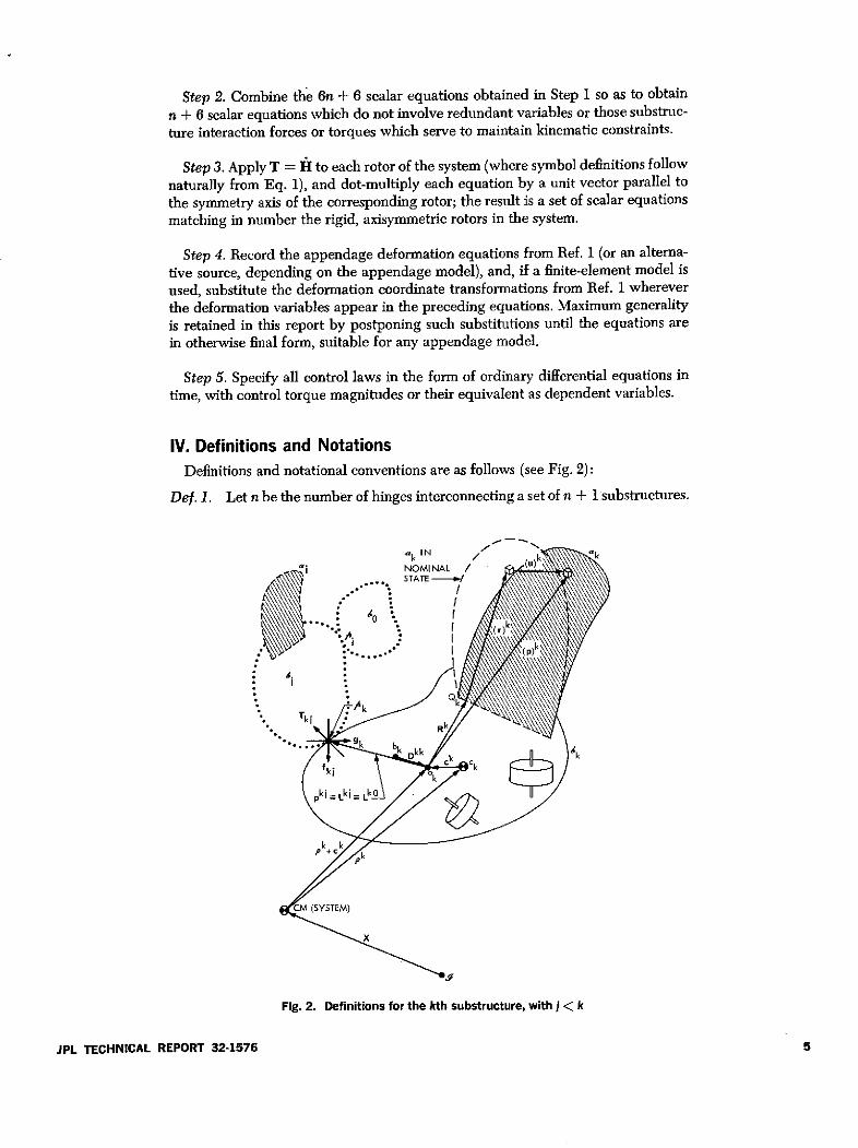
IV. Definitions and NotationsDefinitions and notational conventions are as follows (see Fig. 2):

Def. 1. Let n be the number of hinges interconnecting a set of n + 1 substructures.

a k IN / k 'k

STATE

. /NOMINAL

,kf k j

pkj iLkj- Lk- U

pk+ck

Fig. 2. Definitions for the kth substructure, with i < k


Def. 2. Define the integer set = (0, 1, , n).

Def. 3. Define the integer set = (1, • , n).

Def. 4. Let do be a label assigned to one rigid body chosen arbitrarily as a refer-ence body, and let 6d, - - - , 4n be labels assigned to the rest of the rigidbodies in such a way that if 6, is located between 6o and 4k then 0 < i < k.

Def. 5. Define dextral, orthogonal sets of unit vectors b,b,b so as to be im-bedded in dk for k e 0, and such that in some arbitrarily selected nominalconfiguration of the total system, b" = bi for a = 1, 2, 3 and k, j e 0.

Def.6. Define {b"} _ b kE,3

Def. 7. Define (i) as a column array of inertially fixed, dextral, orthogonal unitvectors il, i2, i3.

Def. 8. Let C be the direction cosine matrix defined by

{bO) = C {i)

Def. 9. Let oO = {(bO)T be the inertial angular velocity vector of 6o, so that o°

is the corresponding 3 X 1 matrix in basis {bO}.

Def. 10. Let Ck be the mass center of the kth substructure, k e 0.

Def. 11. Let /A be a point on the hinge axis common to 4k and ij for j < k and

Def. 12. Let pkJ be the position vector of the hinge point connecting 6i and dkfrom the point o0 occupied by ck when the kth substructure is in its nomi-nal state.

Def. 13. Let c be the position vector from ck to ok.

Def. 14. Let pk be the position vector to ck from the system mass center CM.

Def. 15. Let X be the position vector to CM from an inertially fixed point , andlet X = X({i}.

Def. 16. Let (Mk be the mass of the kth substructure, for k E 3.

Def. 17. Let (p)k be a generic position vector from ok to any point in the kthsubstructure.

Def. 18. Let Qk be a point common to rigid body dA and flexible appendage ak.

Def. 19. Let R' = (bk}T R be the position vector fixed in k locating Qk withrespect to ok.

Def. 20. Let (r)k = (b k} (r) be a generic symbol such that R + (r)k locates atypical field point in ak with respect to ok when the flexible appendage isin some nominal state (perhaps undeformed). For a discretized appendageak, let (rs) k = {bo}T (r)k locate the sth node in the nominal state.


Def. 21. Define the generic deformation vector (u)k in such a way that2

(p)k = Rk + (r)k + (u)kand

(p)k = Rk + (r) + (u)'

For a discretized appendage ak, let (u')t = {bk}T (u')k be the deformationvector for node s.

Def. 22. Let g" ( {bk}T gk be a unit vector parallel to the hinge axis through /k.

Def. 23. For k E 9, let yk be the angle of a gk rotation of dk with respect to the bodyattached at/p k. Let yk be zero when bk = bi (a = 1, 2, 3; f, k E 0).

Def. 24. Let J' =. {bk)T k {bk} be the inertia dyadic of the kth substructure for ok,so that Jk is time-variable by virtue of deformations.

Def. 25. Let Fk = (bk}" Fk be the resultant vector of all forces applied to the kthsubstructure except for those due to interbody forces transmitted at hingeconnections.

Def. 26. Let Tk {bk}T Tk be the resultant moment vector with respect to ck of allforces applied to the kth substructure except for those due to interbodyforces transmitted at hinge connections.

Def. 27. Let rk be the scalar magnitude of the torque component applied to 4k inthe direction of gk by the body attached atf/k.

Def. 28. Let F = F k = {bo}T F be the external force resultant for the total system.

Def. 29. Define the scalar e,k such that for k E 93 and s E

A 1 if t, lies between o and 4kS0 otherwise

(The n (n + 1) scalars Eak are called path elements.)

Def. 30. Define o( = QMk, the total system mass.

Def. 31. Let Cr' be the direction cosine matrix defined by {b) } = Cri {bf), r, je93.(Note that in the nominal state, C jr = U, the unit matrix.)

Def. 32. Let Nkr denote the index of the body attached to 4k and on the path lead-

ing to 4k, and let Nkk = k. (These are the network elements.) For notationalsimplicity, use Nk for Nko.

Def. 33. For3 r E93 - k, let Lk = p kNr, and let Lkk = 0.

Def. 34. Define D kk - 2 LkiflJ./Qn 1 for kE93.

Def. 35. Let bk be a point fixed in Ak such that Dkk is the position vector of ok withrespect to bk. (This point bk is called the barycenter of the kth substructurein the nominal state.)

2Superscripts on generic symbols such as p, r, and u will be omitted when obvious, as when thesymbol appears within an integrand of a definite integral.

3For notational brevity, the set 0 - (k} is designated 93 - k.


Def. 36. Define (b")DkJ = D = iy + Lkj for k, feY3.

Def. 37. Define the dyadic

Kk .Qn, (~r. D~'U - D 1*kr)

where U is the unit dyadic, and define the corresponding matrix Kk{bk}. Kk {(bk}T.

Def. 38. Define

= Kk + J and kk = {b}k) **. {b1}TDef. 39. Define

'* = -( (D j D kjU - DjkIDkj)with

{b}) * {(b})T = -n (CikDJkCJkDki - DfkDkj T)

Def. 40. Let the system of forces applied to dk by the attached body 4j be equiva-lent to a resultant force fki passing through the labeled point (fi orAk)common to 4d and 4, plus a torque Tki.

Def. 41. Let t' be the kinematical constraint torque applied to 4k by vi, in sucha way that, with Defs. 40, 22, and 27,

Tki = te J + jNk k g - 8

kN1j gJ

where8j,=l and 8j=Ofor=I=j.

Def. 42. Let 09 = {bk}Fo be the inertial angular velocity of dk.

Def. 43. Let 30, be the rth neighbor set for re 9, such that k e9, if 4d is attachedto d,.

Def. 44. Let 93jk be the branch set of integers r such that r E 913 if k = Ni,. Thus3Bei consists of the indices of those bodies attached to 6d on a branch

which begins with 4k.

Def. 45. Let hk be the contribution of rotors in d4 to the angular momentum of the

kth substructure relative to d with respect to ok, and let h'* = hk (bk).

V. Derivations of Vector-Dyadic EquationsIn terms of the indicated definitions, Eq. (1) provides, for the rth substructure

(rIE 3),

F' + 2 f- - Cn, (X + r) = 0 (2)

and, for the kth substructure (k E ,),

T + 2 Tkj + 2 (pkj + c ) X Pj - I = 0 (3)

Here a dot over a vector implies time differentiation in an inertial frame of reference.


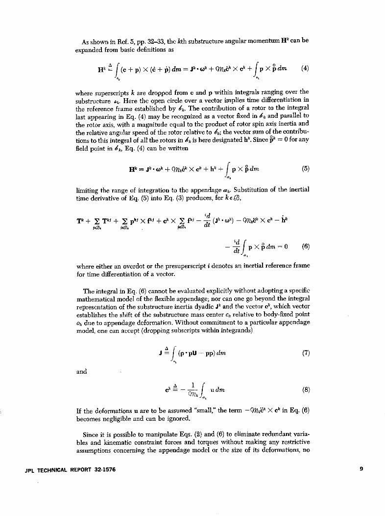
As shown in Ref. 5, pp. 32-33, the kth substructure angular momentum I can be

expanded from basic definitions as

H = (c+p) X(c+p)dm =J ' + k X c + pXpdm (4)

where superscripts k are dropped from c and p within integrals ranging over the

substructure dk. Here the open circle over a vector implies time differentiation in

the reference frame established by k. The contribution of a rotor to the integrallast appearing in Eq. (4) may be recognized as a vector fixed in dk and parallel to

the rotor axis, with a magnitude equal to the product of rotor spin axis inertia and

the relative angular speed of the rotor relative to k; the vector sum of the contribu-

tions to this integral of all the rotors in 4 is here designated hk. Since 0k = 0 for any

field point in 4k, Eq. (4) can be written

Hk = J~. ok + Q k X ck + h + fp X dm (5)

limiting the range of integration to the appendage ak. Substitution of the inertial

time derivative of Eq. (5) into Eq. (3) produces, for k E 9,

T k + I T + p X fk + Ck X f - ) - X - h

i 1d X 0 dm = 0 (6)

where either an overdot or the presuperscript i denotes an inertial reference framefor time differentiation of a vector.

The integral in Eq. (6) cannot be evaluated explicitly without adopting a specificmathematical model of the flexible appendage; nor can one go beyond the integralrepresentation of the substructure inertia dyadic jk and the vector ck, which vectorestablishes the shift of the substructure mass center ck relative to body-fixed point

ok due to appendage deformation. Without commitment to a particular appendagemodel, one can accept (dropping subscripts within integrands)

J f (p pU - pp) dm (7)

and

c k u dm (8)

If the deformations u are to be assumed "small," the term -Qk'dk X Ck in Eq. (6)

becomes negligible and can be ignored.

Since it is possible to manipulate Eqs. (2) and (6) to eliminate redundant varia-bles and kinematic constraint forces and torques without making any restrictiveassumptions concerning the appendage model or the size of its deformations, no


inhibiting assumptions will be imposed until specific cases are considered at theconclusion of this section.

The immediate objective is the extraction from the 6n + 6 equations given byEqs. (2) and (6) of 6 + n equations in the 6 + n unknowns established by the vec-tors X and co and the scalars y , " • • , y' which define the relative rotations of con-tiguous rigid bodies. We must expect these equations also to involve unknowndeformation variables for the appendages and rate variables for the rotors, but wemust eliminate all interaction forces (typified by fki) and all interaction torques(typified by Tki) except for those having the direction of the corresponding hingeaxes, since these hinge-axis torques are known functions of hinge rotation or somemore general control law. We must also eliminate the unknown position vectorstypified by pr, replacing them by explicit functions of the hinge angles -y, - - - , ,and the system geometry, and eliminate all ok for k e 9 in favor of terms involving(o and , for r e 9.

Simply by summing all equations defined by Eq. (2), we obtain the familiar result

F = (Mk(9)

where Ql is the total system mass and F is the resultant of all external forces Fr forre 3. Substituting from Eq. (9) back into Eq. (2) and rearranging produces

F'+ 2 fr' - ,(F/ + ip) = 0SrO,

or, for r e,3,

f'= -F' + O (F/qi + i') (10)

Summing over the branch set 73k (see Def. 44) provides

fk = 2 f8 - [Fr - O q r (F/QC + jr)]

so that, by Newton's third law,

fkP = -fk = [Fr _ q% (F/Gn + ij)] (11)

Substituting Eqs. (10) and (11) into Eq. (6) eliminates all interaction forces fromthe rotational equations, providing

Tk + 2 Tki + 2 pkJ X I [F* - ( , (F/(1 + ir)]

+ cl X [--F + (k(F/97 + i i)] (.k) t (M k X C

dt-h - d pX dm = (ke3) (12)


Equation (12) simplifies when written in terms of the vectors found in Defs. 33-36

in the preceding section, due to the identity, for k E ,

I ep X 2 [Fr -l, (F/q + ij)] = L X [F' - (Mr (F/(7 + Or)]

= O Lkr X Fr + D X F - y Lk" X CM,. r

= (Lk + DI) X Fr - L11 X qijr

= (D' X Fr - L a X Q(M,'i) (13)

Substituting Eq. (13) into Eq. (12) simplifies its appearance somewhat, but there

remains the problem of eliminating the unknown kinematic constraint torqueswhich are present within the interaction torques typified by Tkj. By summing over

all n + 1 vector equations defined by Eq. (12), we can, by virtue of Newton's third

law, obtain one vector equation involving no interaction torques at all; this summa-

tion gives

IT + 2 (D X F' - Lkr X Q,'r) + Ck X [an ( k + F/() - Fk]

td pXtdm} (14)

dt (Jk . ,k) - (ik X ck - hk - p x dm = 0 (14)

Equation (14), like Eq. (9), is free of kinematic constraint forces and torques, sothat these two vector equations can be preserved in the final set that is our objec-tive. The remaining n scalar equations can be obtained by summing equations

obtained from Eq. (12) over branch sets in order to isolate interaction torques such

as Tki, and then by dot-multiplying each expression by the unit vector parallel to

the corresponding hinge axis. In particular, if we introduce the network elements

found in Def. 32 of the previous section, we can sum over the branch set 93N,, andget, for s E 3,

TN, + {T k + (D"' X F' - L k X O ir')

+ c x [On( (j31 + F/On) - F] - dt (J .(0) - ne k X c - h

d- t p X dm =0 (15)

By Def. 32, N, < s, so that the labeled point on the hinge axis common to 0, and

oN, is, by Def. 11, called f/,; the unit vector parallel to the hinge axis is, by Def. 22,called g1; and the interaction torque component of TAN, parallel to gs is, by Def. 27,


.4:k. FOR k W.

cM

Lr c p'rp Lir

Fig. 3. System geometry

called r,. Hence the dot product of Eq. (15) with gS provides the scalar equation,for se o,

, + g* {T + ~ (D' X F7 - L'~' X Qflir) + C X [ Qk (i(i + F/) - F"]

-d ( * " ) - Q' X c - - p PX ) dm = 0 (16)

Equations (9), (14), and (16) provide the required 6 + n scalar equations free ofkinematic constraint forces and torques, but they are not yet in final vector--dyadicform. The variable vectors typified by p7 must first be expressed in terms of thesystem geometry, the deformation variables, and a subset of the 6 + n scalarsrequired to define X, o, and the n angles of relative rotation at the n hinges. As afirst step in this direction, we define @,i as the set of indices of bodies lying on thedirect path between ,r and 4, and then (referring to Fig. 3) we can write

p' - p' = el + L'' + 2 (Lar - Lai) - L J - cr (17)

But L ss = L = 0, by Def. 33, and for any index s in the set 9 - @, the sumL*' - Las = 0, so that Eq. (18) can be written more simply as

p, - p1 = I (Ls' - Lai) + cl _ c' (18)

Multiplying Eq. (18) by (fl/W and summing over all j E,3 produces

Z P' - E ' = Zp ( L - Lai) + Q 1 (ci - C')

But

- p = 0


by definition of CM, and

so we have

pr (L'Z - L) + 1 QfC - C'

Reversing the summation sequence in the first term, changing the index symbol in

the final summation, and substituting the vectors introduced in Defs. 34 and 36, we

find simply that, for r E,

pr= L" + D" + C-- -c = D" + -C-c ) - (19)

Equations (14) and (16) contain not p' itself but combinations which, with Eq. (19),

can be written as

c, X ,iW = nc [ (i" + - - i k (20)

and, in terms employing the symbols of Defs. 33-37,

-2Lk XQn,i = - L'X , D + -Or -X

= - L'X , D' + D5k + - 'd

= I (Dkk - Dkr) X [Qiibkr + CM- (mQ1)]

-2 (nLk X Da - 2 ,L n X D5'r.B-k se-k-r ,Eg-k

= Dkk X l 7 -_ t (n D X ( ,1Dr) + Dkk X 2 CM

- Dkk X 2 "'c6r - (ID Ink)X ,) X cm &

+ Dk' x fti" - C,L' X D""0 O-k sS-0k-r

+ ( Y ,Lk- X b "

rO-k se -r

id= 0 - [ 2 (M,Dk X (o X Iy,)] + 0 - 0 + Dkr X ~Mn,'

dt 't oE$- 2 ,L*' X " + " 2 ,Lk ' X '"rJ-k seM-k-r re-k se3-r


iddt [( 1, (D " * D kU - D'kD'c")} .k]

+ 2lD k r Xl 'r + E E , (L k r - Lks) X Drstwo ral-k seO-r

or

-2 Lk r X 1/r-r =- [K k oC] + CE Q,Dkr X 4as dt ,,g

+ 2 EQn8s (Lkr - Lk-) X D'" (21)TWO -k WO1

In the development leading to Eq. (21), it was recognized that

E (MDr = 0

(reflecting the significance of the barycenter as the mass center of the undeformedaugmented body, which consists of the substructure augmented at each connectionpoint by a particle having the mass of the 'corresponding branch set). It was alsonoted that

-2 1 Q,L k' X X = -kI 2rLk X D8"ret3-k seMJ-k-r sea3-k ret3-k-s

= - (,2 Lk. X DrSre -k smJ-k-r

where the second step involves simply relabeling indices.

Finally, we can recognize in Eq. (21) that the quantity Lk* - LkS is zero for anyindex s corresponding to a body which lies anywhere on the branch which beginswith 6 rN, and includes d,, and for any other index the quantity D18 is also Drk. Thus,in Eq. (21), D'* can be replaced by jrk, with the consequence

id- Lkr X Q - (Kk k) + q D k ' X'"d,( d t ,

+ 2 (,, (L ' - Lk ) X Df rk

mO-k seM

- (K k* (,k) + fo2 , 8X 'c

+ 2 [(ML' - '8 Lk ) X Dk]

or, with Defs. 34 and 36,

- Lkr X Qpr = (Kk * ) + 2 (rDkr x 'r -+ (Dkr X i " (22),oT( f rdt3-k

By substituting Eqs. (20) and (22) into Eqs. (14) and (16), we can obtain thedesired vector-dyadic equations. In this substitution, it becomes apparent that Kk


and Jk always appear in combination, suggesting the introduction of the new dyadicOk0 (see Def. 38). Then the new versions of Eqs. (14) and (16) become

Tk + E Dr X Fr + e X all F - F"k + r CD k X b,

kak

W k t+(. (kl;.k) + 2 G(qkr X Xrk -hk

dtif p 'Xidm =0 (23)

and, with judicious use of the path elements found in Def. 29,

T,+g,*2 k T k+ E DDk' X F' + Ck X F - F

+ E fDk' x y + oMkC X (D rk + (Mr) r id ( "kk)

'dt

+ 2 (D ' X p x ~m =dm 0 (24)

Equations (23) and (24) can be restated in more useful form by expanding termsinvolving time derivatives relative to inertial space to obtain time derivatives rela-

tive to reference frames established by individual substructures, plus additionalundifferentiated terms. In particular, noting that Drk is fixed in 4, we can substitute

brk = & X Dk + C X (car X Dk) (25)

so that in terms of Def. 39, we have

S(MD " X iD'k = - 2 'Dk . ~r + Cf I Dkr X [Or X (O.r X D'k)] (26)re1-k ftM3-k re-- k

The parallel expression for 8' becomes

'd' = 0r + 20' X , + O' X c' + )r X (oC X c') (27)

with open circles representing time differentiation in the reference frame estab-lished by d,.

Other time differentiations in inertial space expand as

h = hk + wk X hk (28)

dt


and

id p x dm=f pX ×dm+ 0Xf (p X ) dm (30)

with the open circle indicating time differentiation in the reference frame estab-lished by the local substructure (here 4k).

By combining Eqs. (23-30), we can obtain the vector-dyadic equations of rota-tion in the form

. Wk = 0 (31)

and

r, + g8 . E,kWk = 0 (32)keg

where

Wk T Tk+ED k' X F' + c X F -F "

+ n,JDk' X r"' + 2c0 X ~" + 6r X c' + c'r X (o' X cr)]

+ f"kce X 2 [6) X D"k + O X (ca X Drk)]

+ Qirek x +-( [ +C X + 6r X C + o X (C' X Cr)] - 4kk• 6k

- Z (Dkr0.)+t~ 2 D k"X ['r X (Or X D'r)]-k X kk. ' k

?Ea73-& r6-k

- hk -- Pk X h kk .gk p dm- (p X -) dm (33)

To obtain the vector-dyadic equations in their final form, involving the 6 + nunknowns in X, Wo, and -y, , y, , as well as the rotor momentum variables andthe deformation variables, we must substitute in Eq. (33) the expressions

0o = o + 2 Eri-rg (34)

and

6c = 6o + 2 er [yr,g + c0o X ,gr + E E,8r,,g X gr] (35)

where Erk are the path elements found in Def. 29, and Defs. 9, 22, and 23 are alsoemployed.

In combination, Eqs. (9) and (31-35) provide the final form of the vector-dyadicequations of vehicle translation and substructure rotation. In addition to theseequations, for each rotor in the system an additional scalar unknown is introduced,and one more differential equation is required. If a rigid axisymmetric rotor withspin axis inertia o, spins relative to body k at the angular rate ck, about an axisparallel to the unit vector b k fixed in 4k, and if T", is the magnitude of the b k com-


ponent of the torque applied to the rotor, then the required additional equation of

motion is

-s, =c , (;'t, + bk *&k) (36)

If there are Nk rotors in lk, and N R rotors in the entire system, then Eq. (36) appliesfor s = 1, - - - , N, with k E 3, so that Eq. (36) contributes NR scalar equations.

Moreover, the variables in equations typified by Eq. (36) are related to those in

Eq. (33) byNk

h = E 6~4~kbk

8 (37)8=1

The scalars typified by 4, must of course be given, either explicitly or implicitlyin the form of additional differential equations representing control laws. The same

is true of rT, Tk, and F r in Eqs. (33) and (32). Once these issues are settled, however,there remains the problem of defining the nonrigid appendages mathematicallyand establishing their vibrational motion equations. This issue has been postponeduntil the end of this section, in order that we might consider several possibilities.The relative advantages of alternative appendage models are considered in detail

in Ref. 6 and are only briefly summarized here.

If the appendage ak is of extremely simple configuration (such as a uniform elastic

beam), and the nominal angular velocity C, of the base to which it is attached is of

a special class (such as zero, or parallel or orthogonal to the hypothesized beam),then it might become attractive to model the appendage as an elastic continuum,writing partial differential equations of vibration, seeking normal modes of vibra-tion, and truncating to a modest number of coordinates and a corresponding num-ber of ordinary scalar differential equations. One must then return to those termsin Eqs. (31-35) which depend on deformation (noting Eqs. 7 and 8) and evaluatethose terms as functions of the modal deformation coordinates, ignoring seconddegree terms in deformation variables.

In most cases, it will prove more feasible to adopt for an elastic appendage afinite-element model such as that described in Section I. The equations of smallvibratory deformation can then be recorded from Ref. 14 (see Eq. 64), and theappropriate coordinate transformation can be adopted from Ref. 1 (see Eq. 74).The vector ck in Eq. (8) is then replaced by c as recorded in Ref. 1, Eq. (43), withe= 0 and summation extending only over the kth substructure. Although thedyadic Jk in Eq. (7) and the integral

Sp X 0 dm

are not provided in Ref. 1, which treats the distributed-mass finite-element modelwith nodal bodies, they are available in Ref. 5 for the special case with all massconcentrated in the nodal bodies; see Ref. 5, Eq. (126) for J1 and Eq. (127) for Jk,

and see Eq. (112) or Eq. (114) for

d-dt pX dm

4Note that the vector called X in Ref. 1 must be interpreted for the rth appendage of the presentpaper as X + pr, with pr expanded as in Eq. (19).


recognizing in each case that the superscript k indicates restriction to the kth sub-structure, and setting Sla and as found in Ref. 5 identically to zero. In each casethe indicated expressions involve deformation variables which must be subjectedto coordinate transformations and truncations, as indicated in Refs. 1 and 5.

If it pleases the analyst, he can conceal the complexities of modeling the elasticappendage by simply adopting a symbolic model in terms of mode shapes andnatural frequencies. Then he can rather easily record the equations of vibration(probably using Lagrange's equations with modal coordinates for generalizedcoordinates), and he can evaluate the deformation-dependent terms in Eqs. (31-33)in terms of unspecified mode shapes and frequencies. Of course he must face theproblems of adopting an appendage model and determining its modal character-istics when he wants to face any real problem.

VI. Matrix EquationsThis section illustrates the transition from the preceding vector-dyadic equa-

tions to an alternative matrix form which is more explicit and therefore more suita-ble for programming for digital computer numerical integration. To obtain explicitresults, we must make a commitment to a particular appendage model, sacrificingsome of the generality of the vector-dyadic equations. In what follows, we confineattention to the special case of the finite element appendage model in Ref. 1 forwhich all mass is concentrated in the n nodal bodies of the system (with no dis-tributed mass for the internodal elastic elements). All deformations from a nomi-nal appendage state are assumed arbitrarily small, so that terms above the firstdegree in these deformations and the corresponding deformation rates can beneglected. Moreover, we assume that only the reference body 6o contains rotors,and these number three, establishing an orthogonal triad whose axes parallel b°, b° ,

and bo. The restrictions adopted in this section reduce the number of terms appear-ing in the final equations of motion somewhat, but (as shown in Ref. 1) they do notchange the structure of the equations, so that the special case treated here remainsrepresentative of the general case of small-vibration appendages. (Large-amplitudeappendage vibrations, which are accommodated in the preceding vector-dyadicequations, would produce matrix equations quite different from those to berecorded here.)

The vector-dyadic equations to be written in matrix form are Eqs. (9) and (31-35),in combination with Eq. (64) of Ref. 1, with various results substituted from Refs. 1and 5.

Equation (9) may be rewritten in terms of Defs. 8, 15, and 28 as

(i}T CT F = (i)T "x

which implies the matrix equation

F = (QCX (38a)

The time history of the direction cosine matrix C is established by the Euler-Poissonkinematic equation (see Ref. 5, Eq. (44), for tilde convention).

C = - C (38b)


Skipping next to the rotor equations and noting the restriction to the three orthog-onal rotors in do (so that k = 0 only, and bo = bo for s = 1, 2, 3), we have from

Eq. (36) the three scalar equations

L = jos ( 'o + o)

or the implied matrix equation

7"R J ( + ,o) (39)

where _ ['ol o02 03] and fis a diagonal matrix with diagonal elementsol, o2,

and 4o3.

The vector rotational equations are easily written in matrix form with the

definition

Wk W* -{b)

since then, in terms of the direction cosine matrices in Def. 31, we can write

Eqs. (31) and (32) as

Z {b }k'W = {bO}r CokW = 0

or simply

SCokW = 0 (40)

and

r, + g'T (b} ' e, E {bk}T Wk = 0

or

T, + g8 " -kCkWk = 0 (41)

Equations (40) and (41) require Wk, which is available from Eq. (33) when writ-ten in the form

(bk)TWk = {bk) T Tk + E {bk} T D X {b,)T F

+ E /tr {bk)T Dkr X {b r)T [Fr + 2~ '+'c + 7Zrc']

+ GM, {b k} ck X {br})T [rDrk + 7r~rDr ] - {b }T e kreo

+ E {(n [Drk' (br) {bk) T Dkr {bk}T U {b k)

rfO-k

- {br) T DrDkrT {bk] (b) {b'r " r}

+ L E [(bk}TDDk X {b'})T rD 'k] - {b k)T' ok k

rfO-k

- {b)}hk - {bk) T hk - ({bk)T fjfidm - ({bk)Tf fdm


since then

W* = (b}. {b11} W

= T + c DkrCkrFr' + CoF - F)

+ 2 (n,bDk Ck (5r + ar6r, + rcr + ZrVc,)

+ QnYnk 2 Ckr (O'Drk + "zroDk) -- 4kk(k _ ,kkk

+ (M I [(Dr'Cr"Dk'U - CkrD'kDk'T) Ck 'reO-k

+ DkCk-.WrDr]

- k - h - lh - " dm - z dm (42)

Even with the substitution of Eq. (42) into Eqs. (40) and (41), the matrix equa-tions are not in their final form, since the variables (

O, )k, hk, ck, ik the directioncosine matrices such as Ckr, and the integrals over ak are not yet sufficiently explicit.These deficiencies are rectified by substituting matrix versions of Eqs. (34), (35),(37), (8), and (7), together with new expressions for Ckr and expressions for theintegrals obtained from Ref. 5. Specifically, from Eqs. (34) and (35), we find

k = {b}.k {bk).=}{bO)r o° + erki ,{br) T gr]rf

or

to = Cko o + 2 EkjCkrgr (43)

and

;= (bk)} = (b k) {bo0 T o

+ 2 Erk [; {b[ (bk} (b)T g + {b)* {b( )T~o X {b)'} gr

+ {b}k) e8,y8 {b')Trg X {b'} T gr]

or

k = CkOo + 2 erk [yCkrgr + Cko(CO,'g, + E es,,sC 'C'g' ] (44)reg seg

For the special case at hand, Eq. (37) yields h_ 0 for k 0 and

ho = {bo) *ho =6G (45)

as these symbols are defined following Eq. (39).


For the nodal body system to which this section is limited, Eq. (8) becomes a

special case of Eq. (45) of Ref. 1 or a variant of Eq. (60) of Ref. 5. Specifically,we have

nk

ck" = - US (46)s=1

where appendage ak has been idealized as nk nodal bodies interconnected by mass-

less elastic structure, with m, the mass of nodal body s and us" [us us uS]T given

by u8 {b")} u with u8 the displacement of the body s relative to ae from the

position occupied in the nominal state.

Recalling from Defs. (38), (37), and (24) that

-Pu = K; + Jk (47)

and noting that Kk is constant and Jk is available from Eq. (7) as the variable matrix

PC f (prpU - ppT ) dm

one can, for the presently adopted appendage model, evaluate Jk as (see Ref. 5,Eq. (126))

Jk = Jk + 2 (m, [2 (Rk + rs)T usU - (Rk + r8) us' - u8 (Rk + rS)T] + PI8 - P')

(48)

where J, is the nominal (constant) value of Jk, and Is is the constant inertia matrixof the sth nodal body in its own body-fixed vector basis {ns}k, where, in the nominalstate, (ns)k = {bk}. Here we use u8 for (us)k, as in Def. 21.

In combination, Eqs. (47) and (48) provide

. = , (m. [2 (Rk - rS)T U (R + r) i i(Rk+ r8)7] +p818 - IPS) (49)

An expression for the direction cosine matrix CkNk (where k e 9 and N7, is a net-work element from Def. 32) may be found from Ref. 7 to be

CkNk = U cos yk - Rk sin yk + gkgkl (1 - cos yk) (50)

and, by transposition,

CNkk = U cos yk + R sin yk + gkgkT (1 - cos 'k) (51)

For arbitrary r, j E £3, the direction cosine matrix Cri can be constructed as a productof direction cosine matrices relating contiguous bodies (as given by Eqs. 50 and 51).


The required product can be written symbolically as

Cri = 1I~rCkNk (52a)

where the symbol I-Njr is understood to imply the following algorithm:

(1) Define p = N, and construct C' p from Eq. (50) if r > p and from Eq. (51)if r < p.

(2) Define q = Nvi and construct C 7 from Eq. (50) if p > q and from Eq. (51)if p < q.

(3) Proceed until an integer u emerges such that ji N,, finally constructing CUIfrom Eq. (50) if u > j and from Eq. (51) if u < i.

(4) Multiply the matrices obtained in the sequence

C'j = C'pCpq . . Cuj (52b)

Finally, Eq. (42) requires more explicit expressions for the integrals over theappendage ak. For the special case of elastic appendages idealized as intercon-nected nodal bodies, the appropriate expressions can be found in vector form inEq. (114) of Ref. 5. The corresponding matrix equations are

- dm- kf j5l dm= - (-kRk)-+ m

R k (E miis + Zk 2 m'Its) - m ()msi

- 7? (miis + Zkmmstj) Is- 21(f + ;kfs)

- zk Z Js/3 + E

S- (lk + ?) msiis - k (Rk + 7) mis

- y [1s () + Zk.s) - ZP1Ps + 1%k/] (53)

where E implies summation over the range from s = 1 to s = n, and the super-script k has been dropped from nodal body variables in the kth appendage (suchas us, which replaces (us)k). In developing Eq. (53), the identity (ab)~ = ab - bihas been utilized.

In summary, in order to obtain the explicit matrix equations defining substruc-ture rotations, one must combine Eqs. (42-53) into Eqs. (40) and (41). The result isa set of n + 3 scalar equations, which can be collected together with the three rotorequations (Eq. 39) and the three vehicle translation equations (Eq. 38a) and theirkinematic equations (Eq. 38b) to comprise a set which is complete except for con-trol system equations and the equations of vibration of each of the n + 1 append-


ages. The latter set can be obtained for a distributed-mass finite-element model

from Eq. (64) of Ref. 1, and for the special case of the concentrated-mass (nodal

body) finite-element model either from Eq. (64) of Ref. 1 or from Eq. (95) of Ref. 5

(correcting the last algebraic sign within the braces on the right side of Eq. (95) bychanging - to +), recognizing that what is recorded as OX in those equations

must be replaced by the inertial acceleration of the mass center of the correspond-ing substructure in the local vector basis, which for substructure ak is given by

Cx + {b) )- j = CX + {b}) . (D k + -r) - 5k

= Ck - (' + ZkCk + 2-5 + a"c )

+ 2 C k (p + Z ) D'k + "I c") + (5 + 2r)

(54)

where Eq. (19) has been utilized for the expansion of i1.

Typically the number of nodes n, in a single finite-element model of an elastic

appendage is so great that the proposed combination of nodal body vibration equa-tions with substructure rotation equations, vehicle translation equations, rotor

equations, and control system equations would be prohibitive in size for numericalintegrations. Thus it is to be understood at the outset that the nodal body vibration

equations will provide the basis for a transformation to distributed or modal coordi-nates for appendage deformations, and that most of the modal coordinates will bedeleted from consideration by truncating the matrix of deformation variables. Bymeans of this transformation, all variables labeled u8 and P8 in Eqs. (46-53) arereplaced by appropriate combinations of new modal deformation variables. Thusthe equations actually to be programmed for digital computer numerical integra-tion are not precisely those obtained from Eqs. (38-53) of this report plus Eq. (64)of Ref. 1 (or Eq. 95 of Ref. 5), but instead the transformed and truncated versionsof these equations. Because questions of transformation, truncation, and synthesisof the resulting composite matrix equations have been treated extensively in Refs. 1,5, and 8, these matters will not be considered further here.

VII. SummaryBy combining Eqs. (9), (31), (32), and (36) with Eq. (64) of Ref. 1, one can obtain

a generic statement of a minimum dimension set of equations of motion of a systemof n + 1 rigid bodies interconnected by n line hinges, with a set of axisymmetricrotors and a distributed-mass finite-element model of an elastic appendage attachedto each rigid body. In order for these equations to stand alone as a complete formu-lation of the problem, one must substitute the auxiliary equations (33-35) and (37),as well as certain specified equations from Ref. 5, into Eqs. (31) and (32), andEq. (64) of Ref. 1 must be composed from the underlying equations of that ref-erence (Eqs: 46, 53, and 62). Moreover, the total system of equations must forpractical utilization be written in matrix form and the appendage deformationssubjected to modal coordinate transformations and truncations, as these proceduresare described in Refs. 1 and 5 and illustrated in part for a special case in the preced-ing section of this report.


Although one must not underestimate the labors of proceeding from the vector-dyadic equations in this report to a generic computer program for integrating theseequations, this does appear to be a feasible task. Once the program is completed,it will have sufficient generality to encompass several spacecraft simulations forwhich specific numerical integration computer programs have been written in thepast (Refs. 8-10). Experience with these programs provides reasonable assurancethat the generic program proposed here will find application as a practical tool forthe simulation of complex modern spacecraft.

References

1. Likins, P. W., "Finite Element Appendage Equations for Hybrid CoordinateDynamic Analysis," Int. J. Solids Struct., Vol. 8, pp. 709-731, 1972. (Also avail-able in expanded form as Technical Report 32-1525, Jet Propulsion Laboratory,Pasadena, Calif., Oct. 15, 1971.)

2. Hooker, W. W., and Margulies, G., "The Dynamical Attitude Equations for ann-Body Satellite," J. Astronaut. Sci., Vol. 12, pp. 123-128, 1965.

3. Hooker, W. W., "A Set of r Dynamical Attitude Equations for an ArbitraryN-Body Satellite Having r Rotational Degrees of Freedom," AIAA J., Vol. 8,pp. 1205-1207, 1970.

4. Roberson, R. E., and Wittenburg, J., "A Dynamical Formalism for an ArbitraryNumber of Interconnected Rigid Bodies, With Reference to the Problem ofSatellite Attitude Control," Proc. 3rd Int. Congress of Automatic Control(London, 1966), Butterworth and Co., Ltd., London, 1967.

5. Likins, P. W., Dynamics and Control of Flexible Space Vehicles, TechnicalReport 32-1329, Rev. 1, Jet Propulsion Laboratory, Pasadena, Calif., Jan. 15,1970.

6. Likins, P.W., Barbera, F.J., and Baddeley, V., "Mathematical Modeling of Spin-ning Elastic Bodies for Modal Analysis," submitted to AIAA J.

7. Likins, P. W., and Fleischer, G. E., Large Deformation Modal Coordinates forNonrigid Vehicle Dynamics, Technical Report 32-1565, Jet Propulsion Labora-tory, Pasadena, Calif., Nov. 1, 1972.

8. Gale, A. H., and Likins, P. W., "Influence of Flexible Appendages on Dual-SpinSpacecraft Dynamics and Control," 1. Spacecraft Rockets, Vol. 7, pp. 1049-1056,1970.

9. Likins, P. W., and Fleischer, G. E., "Results of Flexible Spacecraft AttitudeControl Studies Utilizing Hybrid Coordinates," J. Spacecraft Rockets, Vol. 8,pp. 264-273, 1971.

10. Fleischer, G. E., and McGlinchey, L. F., "Viking Thrust Vector Control Dy-namics Using Hybrid Coordinates to Model Vehicle Flexibility and PropellantSlosh," AAS/AIAA Paper 71-348, presented at the Astrodynamics Specialists'Conference, Ft. Lauderdale, Fla., American Astronautical Society, 1971.

24 JPL TECHNICAL REPORT 32-1576NASA - JPL - Coml., L.A., Calif.

Documents

Dynamic Analysis of a System of Hinge-Connected Rigid ... · Rigid Bodies With Nonrigid Appendages ... Dynamic Analysis of a System of Hinge-Connected Rigid Bodies With Nonrigid Appendages