DYNAMIC ALLOCATION OF RENEWABLE ENERGY THROUGH ASTOCHASTIC KNAPSACK PROBLEM FORMULATION FOR AN ACCESS

POINT ON THE MOVE

A THESIS SUBMITTED TOTHE GRADUATE SCHOOL OF NATURAL AND APPLIED SCIENCES

OFMIDDLE EAST TECHNICAL UNIVERSITY

BY

ELIF TUGÇE CERAN

IN PARTIAL FULFILLMENT OF THE REQUIREMENTSFOR

THE DEGREE OF MASTER OF SCIENCEIN

ELECTRICAL AND ELECTRONICS ENGINEERING

JUNE 2014

Approval of the thesis:

DYNAMIC ALLOCATION OF RENEWABLE ENERGY THROUGH ASTOCHASTIC KNAPSACK PROBLEM FORMULATION FOR AN ACCESS

POINT ON THE MOVE

submitted by ELIF TUGÇE CERAN in partial fulfillment of the requirements for thedegree of Master of Science in Electrical and Electronics Engineering Depart-ment, Middle East Technical University by,

Prof. Dr. Canan ÖzgenDean, Graduate School of Natural and Applied Sciences

Prof. Dr. Gönül Turhan SayanHead of Department, Electrical and Electronics Engineering

Prof. Dr. Elif Uysal BıyıkogluSupervisor, Electrical and Electronics Eng. Dept., METU

Examining Committee Members:

Prof. Dr. Yalçın TanıkElectrical and Electronics Engineering Department, METU

Prof. Dr. Elif Uysal BıyıkogluElectrical and Electronics Engineering Department, METU

Prof. Dr. Kemal LeblebiciogluElectrical and Electronics Engineering Department, METU

Assoc. Prof. Dr. Melek Diker YücelElectrical and Electronics Engineering Department, METU

Assoc. Prof. Dr. Tolga GiriciElectrical and Electronics Engineering, TOBB ETU

Date:

I hereby declare that all information in this document has been obtained andpresented in accordance with academic rules and ethical conduct. I also declarethat, as required by these rules and conduct, I have fully cited and referenced allmaterial and results that are not original to this work.

Name, Last Name: ELIF TUGÇE CERAN

Signature :

iv

ABSTRACT

DYNAMIC ALLOCATION OF RENEWABLE ENERGY THROUGH ASTOCHASTIC KNAPSACK PROBLEM FORMULATION FOR AN ACCESS

POINT ON THE MOVE

ELIF TUGÇE CERAN,

M.S., Department of Electrical and Electronics Engineering

Supervisor : Prof. Dr. Elif Uysal Bıyıkoglu

June 2014, 67 pages

The problem studied in this thesis has been motivated by recent industry efforts to-ward providing Internet service in areas of the world devoid of regular telecommuni-cations infrastructure via flying or floating platforms in the lower stratosphere. Ac-cording to the abstraction in the thesis, the Access Point on the Move (APOM) havinga renewable energy supply feature (solar, wind, etc.) must judiciously allocate this re-source to provide service to users that demand service from it while it moves over anarea. Within the problem setup, users with various stochastic characteristics (resourcedemands or rewards) appear in a sequential manner and the APOM must make onlinedecisions whether or not to provide service to each appearing user. The objective ofthe APOM is to maximize a total utility (reward) provided to the encountered users.The problem is formulated as a 0/1 stochastic knapsack problem with stochasticallygrowing dynamic capacity, solution of which is not available in previous literature.In this thesis, dynamic and stochastic policies are proposed considering the cases ofboth finite and infinite problem horizons. A threshold based policy based on dynamicprogramming approach is shown to be optimal under some conditions. Taking advan-tage of the structural characteristics of the optimal problem, promising suboptimalsolutions that can adapt to short-time-scale dynamics are proposed and their perfor-mance are analysed in different scenarios. Kalman filtering based prediction of solarenergy to inform online resource allocation policies is also considered.

v

Keywords: Access Point on the move, dynamic resource allocation, decision problem,threshold policy , energy harvesting, dynamic programming, Stochastic 0/1 knapsackproblem, Knapsack with dynamic capacity, Markov Decision Process, ReinforcementLearning, Finite horizon, Infinite horizon, Discount factor

vi

ÖZ

HAREKETLI ERISIM NOKTALARI IÇIN OLASILIKSAL KNAPSACKPROBLEMI FORMÜLASYONU ILE DINAMIK YENILENEBILIR KAYNAK

ATAMASI

ELIF TUGÇE CERAN,

Yüksek Lisans, Elektrik ve Elektronik Mühendisligi Bölümü

Tez Yöneticisi : Prof. Dr. Elif Uysal Bıyıkoglu

Haziran 2014 , 67 sayfa

Son yıllarda endüstriyel alanda telekommünikasyon altyapısı eksik bölgelere internetsaglamak amacıyla stratosferde uçan veya süzülen platformlar gelistirilmeye baslan-mıstır. Bundan hareketle, bu tezde enerji hasatı kabiliyetli (günes, rüzgar vb.) ve Hare-ketli Erisim Noktalarının (HEN) hareket sürecince karsılasacagı kullanıcılara kaynakatama problemi incelenecektir. Problem kurulumunda, ard arda beliren farklı özel-liklere sahip (fayda ve enerji talebi) kullanıcılar için HEN’in çevrimiçi bir sekildeservis verip vermeme kararı vermesi gereklidir. HEN’in nihai hedefi karsılasılan kul-lanıcılardan elde edilecek fayda beklentisini maksimize etmek aynı zamanda enerjikapasitesini asmamaktır. Problem 0/1 olasılıksal knapsack problemi olarak formüleedilebilir. Mevcut enerjinin olasılıksal enerji hasatı ile arttıgı düsünüldügünde, formü-lasyonda kullanılan knapsack problemi dinamik kapasiteye sahiptir. Bu tezde sonluve sonsuz ufuklu durumlar için dinamik ve olasılıksal yöntemler önerilmektedir. Di-namik programlama yaklasımı kullanılarak belirli durumlarda esik bazlı bir yönteminideal oldugu gösterilmektedir. Ideal çözümün yapısal özellikleri göz önünde bulundu-rularak kısa vadeli dinamiklere uyum saglayabilen etkili en iyi altı çözümler önerilipfarklı senaryolardaki performansları incelenmektedir. Ayrıca, kaynak atama yöntem-leri ile birlikte kullanılmak üzere Kalman bazlı günes enerjisi kestirim algoritmasıdegerlendirilmektedir.

vii

Anahtar Kelimeler: Hareketli erisim noktaları, dinamik kaynak atama, karar prob-lemi, enerji hasatı, Olasılıksal 0/1 knapsack problemi, dinamik kapasiteli Knapsack,Markov Karar Süreci, takviyeli ögrenme, sonlu ufuk, sonsuz ufuk, kırdırım katsayısı

viii

to my beloved family

ix

ACKNOWLEDGMENTS

I would like to express my sincerest gratitude to my supervisor Prof. Dr. Elif UysalBıyıkoglu for her excellent guidance, insight, patience and kindness motivated me tocomplete this thesis. All talks and discussions with her was a unique inspiration tome. Her contribution to this dissertation was truly invaluable. Moreover, I take thisopportunity to thank Prof. Dr. Kemal Leblebicioglu and Assoc. Prof. Dr. Tolga Giriciwho I had a chance to work with, for their invaluable support, constructive commentsand attentiveness to weekly discussions through the development of this thesis.

I also would like to thank my friends and colleagues in the METU CommunicationNetworks Research Group and Tugçe Erkılıç for their generous help and preciousfriendship.

I would like to acknowledge the Scientific and Technological Research Council ofTurkey(TÜBITAK) for their financial support during my graduate study.

Last but not the least, I would like to thank to my beloved parents Ümran and Bilal andmy brother Salih. I am indebted to them for their everlasting support, encouragementand sincere prayers. I also would like to express my heart-felt gratitude to my friendsNazan, Öykü, Günce and Serhat for their patience and love.

x

TABLE OF CONTENTS

ABSTRACT . . . . . . . . . . . . . . . . . . . . . . . . . . . . . . . . . . . . v

ÖZ . . . . . . . . . . . . . . . . . . . . . . . . . . . . . . . . . . . . . . . . . vii

ACKNOWLEDGMENTS . . . . . . . . . . . . . . . . . . . . . . . . . . . . . x

TABLE OF CONTENTS . . . . . . . . . . . . . . . . . . . . . . . . . . . . . xi

LIST OF TABLES . . . . . . . . . . . . . . . . . . . . . . . . . . . . . . . . xiv

LIST OF FIGURES . . . . . . . . . . . . . . . . . . . . . . . . . . . . . . . . xv

LIST OF ABBREVIATIONS . . . . . . . . . . . . . . . . . . . . . . . . . . . xvii

CHAPTERS

1 INTRODUCTION . . . . . . . . . . . . . . . . . . . . . . . . . . . 1

2 BACKGROUND INFORMATION . . . . . . . . . . . . . . . . . . . 5

2.1 A Review on the Efficient Resource Allocation in EnergyHarvesting Wireless Networks . . . . . . . . . . . . . . . . 5

2.1.1 A Review on Energy Harvesting and Energy Har-vesting Systems . . . . . . . . . . . . . . . . . . . 5

2.1.2 A Review on Dynamic Resource Allocation in Wire-less Networks with Energy Harvesting . . . . . . . 8

2.2 A Review on Knapsack Problems . . . . . . . . . . . . . . . 9

2.2.1 Knapsack Problems and NP-hardness . . . . . . . 9

xi

2.2.2 Observations and Methods . . . . . . . . . . . . . 11

2.3 A review on the Deterministic Knapsack Problem with In-cremental Capacity formulation of the Resource AllocationProblem in Wireless Access Point on the Move . . . . . . . . 14

3 PREDICTION BASED DYNAMIC RESOURCE ALLOCATION INENERGY HARVESTING WIRELESS NETWORKS WITH A FIXEDTRANSMITTER . . . . . . . . . . . . . . . . . . . . . . . . . . . . 17

3.1 Solar Energy Prediction based on Discrete Kalman Filter . . 18

3.2 Proportional Fair Resource Allocation Algorithm with Of-fline Knowledge of Energy Harvest . . . . . . . . . . . . . . 22

3.3 Performance Evaluation and Numerical Results . . . . . . . 24

4 FINITE HORIZON DYNAMIC EXPECTED UTILITY MAXIMIZA-TION UNDER ENERGY CONSTRAINTS . . . . . . . . . . . . . . 31

4.1 System Model and Problem Statement . . . . . . . . . . . . 31

4.1.1 System Model . . . . . . . . . . . . . . . . . . . . 31

4.1.2 Problem Statement: Finite Horizon . . . . . . . . . 34

4.2 Optimal Online Solution with Dynamic Programming . . . . 36

4.3 Structure of the Optimal Policy . . . . . . . . . . . . . . . . 40

4.3.1 Existence of Threshold . . . . . . . . . . . . . . . 41

4.3.2 Monotonicity of Threshold . . . . . . . . . . . . . 43

4.3.3 Curse of dimensionality . . . . . . . . . . . . . . 45

4.4 Suboptimal Solution: Expected Threshold Policy . . . . . . . 46

4.5 Performance Evaluation and Numerical Results . . . . . . . 48

5 INFINITE HORIZON DYNAMIC EXPECTED UTILITY MAXI-MIZATION UNDER ENERGY CONSTRAINTS . . . . . . . . . . . 53

xii

5.1 System Model and Problem Statement . . . . . . . . . . . . 53

5.1.1 System Model . . . . . . . . . . . . . . . . . . . . 53

5.1.2 Problem Statement of Maximizing Mean Reward . 54

5.1.3 Problem Statement of Maximizing Discounted Ex-pected Reward . . . . . . . . . . . . . . . . . . . 55

5.2 Optimal Online Solution with Dynamic Programming . . . . 55

5.2.1 Markov Decision Process . . . . . . . . . . . . . . 55

5.3 Suboptimal Online Policy . . . . . . . . . . . . . . . . . . . 57

5.3.1 Suboptimal Online Solution: Renewal Modelling . 57

5.3.2 Suboptimal Online Solution: L-Level LookaheadPolicy . . . . . . . . . . . . . . . . . . . . . . . . 57

5.4 Performance Evaluation and Numerical Results . . . . . . . 59

6 CONCLUSION . . . . . . . . . . . . . . . . . . . . . . . . . . . . . 61

REFERENCES . . . . . . . . . . . . . . . . . . . . . . . . . . . . . . . . . . 63

xiii

LIST OF TABLES

TABLES

Table 2.1 An Overview of Previous Studies . . . . . . . . . . . . . . . . . . . 13

Table 3.1 Average Over 14 Frames of 3 Gateways’ Throughputs (Gigabytes/day) 27

Table 5.1 Performance Evaluation of L-level Heuristic with Respect to Opti-mal Based on DP for Different Values of Discount Factor, γ . . . . . . . . 59

xiv

LIST OF FIGURES

FIGURES

Figure 1.1 Recent industrial efforts toward putting ISP’s in the Earth’s atmo-sphere, e.g. Google Loon Project [1] . . . . . . . . . . . . . . . . . . . . 2

Figure 1.2 Recent industrial efforts toward putting ISP’s in the Earth’s atmo-sphere, e.g. Facebook Drone Project [24] . . . . . . . . . . . . . . . . . . 2

Figure 2.1 Markov model for energy harvests . . . . . . . . . . . . . . . . . . 7

Figure 3.1 One of the multiple frames in a timeline. The highlighted frame,frame i (of 24 hours), includes K energy arivals. The time between con-secutive arrivals is allocated to N users [16]. . . . . . . . . . . . . . . . . 18

Figure 3.2 Performance of K-SEP with respect to the real measurements pro-vided by the University of Oregon Solar Radiation Laboratory; belongingto 07.05.2009-19.05.2009 for Salem, MA, USA. . . . . . . . . . . . . . . 24

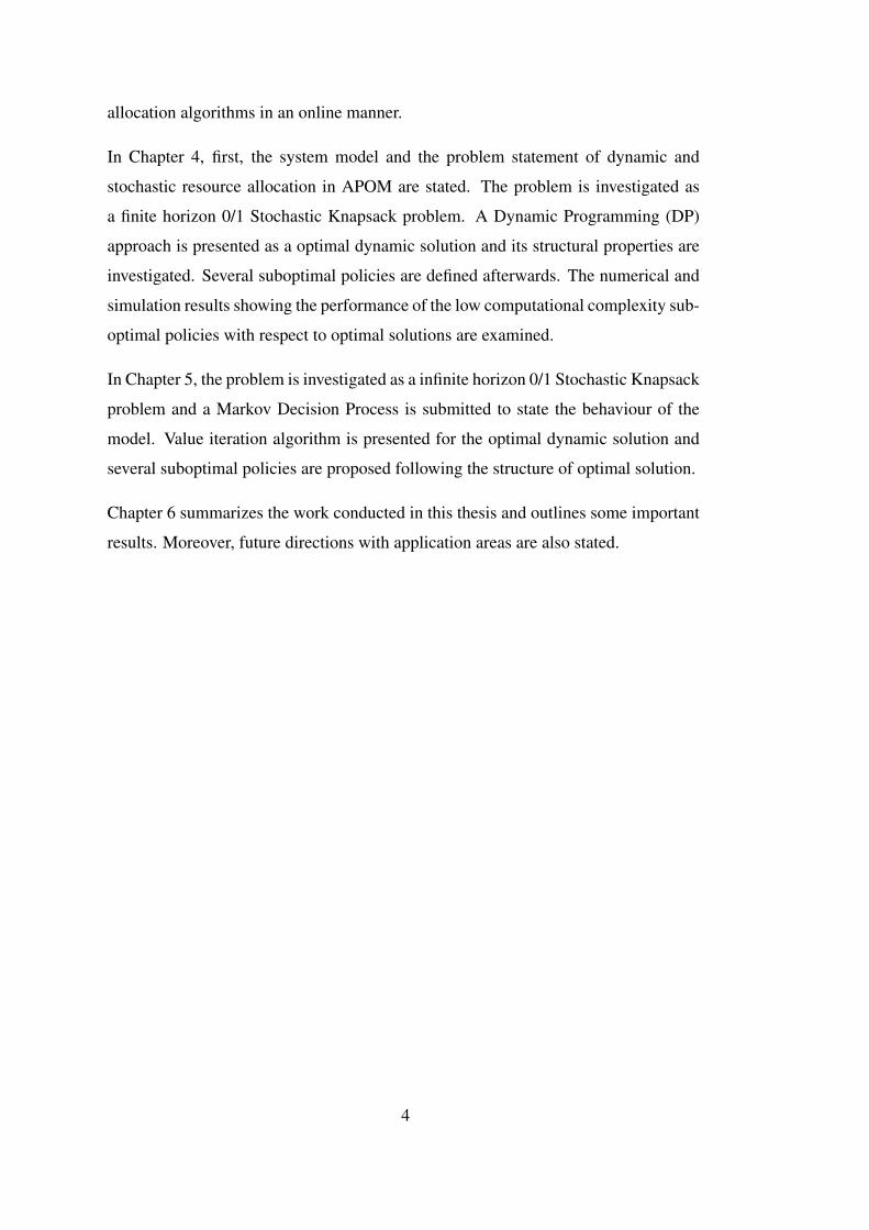
Figure 3.3 Performance of K-SEP with respect to the real measurements pro-vided by the University of Oregon Solar Radiation Laboratory; belongingto 01.01.2011-13.01.2011 for Salem, MA, USA. . . . . . . . . . . . . . . 25

Figure 3.4 Performances of K-SEP and S-SEP compared with the real powermeasurements provided in [48]; belonging to 16.10.2009 for Amherst,MA, USA [16]. . . . . . . . . . . . . . . . . . . . . . . . . . . . . . . . 26

Figure 3.5 Performances of K-SEP and S-SEP compared with the real powermeasurements provided in [48]; belonging to 10.10.2009 for Amherst,MA, USA [16]. . . . . . . . . . . . . . . . . . . . . . . . . . . . . . . . 26

Figure 3.6 Performances of K-SEP and S-SEP compared with the real powermeasurements provided in [48]; belonging to 04.10.2009 for Amherst,MA, USA [16]. . . . . . . . . . . . . . . . . . . . . . . . . . . . . . . . 27

Figure 3.7 Utility and Throughput Improvements of PTF and PTF-On overSG+TDMA on Amherst, MA solar irradiation data. . . . . . . . . . . . . 28

xv

Figure 3.8 Total Throughput of the three gateways (in Gigabytes) over 14Frames on Amherst, MA solar irradiation data. . . . . . . . . . . . . . . . 28

Figure 4.1 Overall system model of APOM with renewable energy sources . . 32

Figure 4.2 The performance evaluation of Expected Energy Threshold Heuris-tic wrt. Optimal Policy when available energy=10, N = 20, K = 2 fortwo different user types with efficiency ratios 10 and 5 . . . . . . . . . . . 49

Figure 4.3 The performance evaluation of Expected Energy Threshold Heuris-tic wrt. Optimal Policy when available energy=5, N = 20, K = 2 for twodifferent user types with efficiency ratios 10 and 5 . . . . . . . . . . . . . 49

Figure 4.4 The comparison of the performances for Expected Energy Thresh-old Policy, Greedy Policy and Conservative Policy with respect to OptimalPolicy when available energy=5, N = 100, K = 2 for two different usertypes with efficiency ratios 10 and 5 (best users appearing with high prob-ability e.g. 0.7) . . . . . . . . . . . . . . . . . . . . . . . . . . . . . . . 50

Figure 4.5 The comparison of the performances for Expected Energy Thresh-old Policy, Greedy Policy and Conservative Policy with respect to OptimalPolicy when available energy=5, N = 100, K = 2 for two different usertypes with efficiency ratios 10 and 5 (worst users appearing with highprobability e.g. 0.7) . . . . . . . . . . . . . . . . . . . . . . . . . . . . . 51

Figure 4.6 The comparison of the performances for Expected Energy Thresh-old Policy, Greedy Policy and Conservative Policy with respect to OptimalPolicy when available energy=5 at the beginning, N = 100, K = 5 forfive different user types with equal weights . . . . . . . . . . . . . . . . . 52

Figure 4.7 The comparison of the performances for Expected Energy Thresh-old Policy, Greedy Policy and Conservative Policy with respect to OptimalPolicy when available energy=5 at the beginning, N = 100, K = 5 forfive different user types with different efficiency (value/weight) ratios anddifferent weights . . . . . . . . . . . . . . . . . . . . . . . . . . . . . . 52

Figure 5.1 The overall system model for APOM with random energy harvest-ing intervals . . . . . . . . . . . . . . . . . . . . . . . . . . . . . . . . . 54

xvi

LIST OF ABBREVIATIONS

ABBRV Abbreviation

AP Access Point

APOM Access Point On the Move

DP Dynamic Programming

DSKP Dynamic and Stochastic Knapsack Problem

KP Knapsack Problem

KSEP Kalman Based Solar Energy Prediction

MDP Markov Decision Process

xvii

xviii

CHAPTER 1

INTRODUCTION

In the era of communication, access to information via Internet is gradually becoming

more and more crucial. However, a lot of people on the planet are completely devoid

of connectivity because of a remote locale, a lack of infrastructure, a coverage gap

and, in some cases, a combination of all tree. Motivated by this fact, recently, major

industry players have been pushing for ubiquitous Internet access, because of the large

potential increase to their businesses from including users from areas of the world that

are still devoid of connectivity. Among all the possible solutions for increasing the

pervasiveness of the Internet, the trend of putting mobile Internet service providers

(ISP) in the Earth’s atmosphere (e.g. Google Loon Project[33] and Facebook Drones

[36]) is a novel and promising technology.

There have been a significant amount of studies regarding mobile sinks in conven-

tional networks, not considering renewable energy sources [17],[42],[50]. Further-

more, the advantages of mobile service providers over fixed providers has been shown

in previous studies [50], [56]. Some of the these studies focused on determining the

optimal path in order to prolong network lifetime [30],[22]. Alkesh et al. [4] proposed

a fuzzy logic strategy to select cluster heads of a network and tried to maximize the

lifetime of wireless sensor networks with limited batteries.

In addition to the mobility advantage of Access Points (AP), to achieve self-sustainable

and environmentally friendly development of service providers, AP’s should be pow-

ered with renewable energy devices that harvest its own energy, e.g., solar or wind

power. The recent advances in the area of energy scavenging enable communication

devices with not only low carbon footprint, but also high performance give us the op-

1

Figure 1.1: Recent industrial efforts toward putting ISP’s in the Earth’s atmosphere,

e.g. Google Loon Project [1]

Figure 1.2: Recent industrial efforts toward putting ISP’s in the Earth’s atmosphere,

e.g. Facebook Drone Project [24]

2

portunity to design such a system. Hence, Access Point on the Move (APOM) with

the capability of energy harvesting from renewable energy sources (solar, wind etc.)

is a viable solution to provide ubiquitous Internet to the users in different areas around

the world.

However, an APOM with limited capacity of energy and high amount of service re-

quests encounters with a well known problem of resource allocation. Resource man-

agement is very critical in Information and Communication Technologies (ICT), es-

pecially for the industrial applications like APOM [52]. Considering the case, where

there are multiple Access Points (APs) working as routers and communicating with

each other in the area of coverage, an AP should decide which users to be served

by the current router or deferred to get service from the next router during its route.

The deterministic version of the problem has been extensively analysed in [11] that

proposes several online heuristics to maximize total utility regarding energy causality

constraints in a deterministic environment.

On the other hand, exploiting the uncertainty of both the environment and user char-

acteristics in the real life conditions, the problem is formulated as a dynamic and

stochastic resource allocation problem in which utilities and resource demands asso-

ciated with the appearing users and energy capacity changes in a probabilistic manner.

The stochastic and dynamic setup of the problem is quite realistic since energy har-

vesting is actually a stochastic event [58], and channel conditions randomly change

in time [7]. To the best of our knowledge, maximizing the total expected utility sub-

ject to energy capacity constraints in a mobile AP with energy harvesting is still a

quite open problem. Hence, the main aim of this thesis is to introduce the problem

of dynamic and stochastic resource allocation in AP’s with movement and energy

harvesting capability and to investigate some optimal and suboptimal solutions.

This thesis is divided into 6 chapters. In the following chapter, Chapter 2, recent

developments in the resource allocation of mobile routers are reviewed and a detailed

background on previously defined Knapsack problems and related solutions are given.

Solutions from the literature as well as those proposed by us are introduced. The

main contribution of this thesis are given in the Chapters 3, 4, 5. First, a Kalman filter

based solar energy prediction method (KSEP) is introduced to be used with resource

3

allocation algorithms in an online manner.

In Chapter 4, first, the system model and the problem statement of dynamic and

stochastic resource allocation in APOM are stated. The problem is investigated as

a finite horizon 0/1 Stochastic Knapsack problem. A Dynamic Programming (DP)

approach is presented as a optimal dynamic solution and its structural properties are

investigated. Several suboptimal policies are defined afterwards. The numerical and

simulation results showing the performance of the low computational complexity sub-

optimal policies with respect to optimal solutions are examined.

In Chapter 5, the problem is investigated as a infinite horizon 0/1 Stochastic Knapsack

problem and a Markov Decision Process is submitted to state the behaviour of the

model. Value iteration algorithm is presented for the optimal dynamic solution and

several suboptimal policies are proposed following the structure of optimal solution.

Chapter 6 summarizes the work conducted in this thesis and outlines some important

results. Moreover, future directions with application areas are also stated.

4

CHAPTER 2

BACKGROUND INFORMATION

A detailed background information on the subject of this thesis is outlined in this

chapter. First, some previous studies about the resource allocation for both fixed and

mobile service providers including the cases with both conventional and renewable

energy sources is summarized. Then, a background information related to the general

Knapsack problems which will be used to model the resource allocation problem in

this thesis and their applications are provided.

2.1 A Review on the Efficient Resource Allocation in Energy Harvesting Wire-

less Networks

2.1.1 A Review on Energy Harvesting and Energy Harvesting Systems

Recently, employing energy harvesting (via ambient energy sources such as solar

irradiation [9], vibrations [37], [45], and wind [57]) to power transmitters of wireless

networks, such as APs has gained tremendous interest [2]. Today, especially solar

energy is becoming widely used, due to its high power density compared to other

sources of ambient energy [38]. With the development of high performance and low

carbon-footprint energy scavenging devices, the main aim in the energy allocation

to different tasks becomes to adapt the energy consumption of a transmitter to the

energy harvesting characteristics. A conservative approach in energy allocation will

cause the energy storage costs not to mention the low utility, on the other hand, a

greedy approach will result in inefficient use of resources and reduces the total reward.

Therefore, nowadays, the focus of the research community has been changed into

5

providing energy neutrality in wireless networks rather than low energy consumption

to design energy efficient communication systems.

Energy harvesting systems do not instantly consume the energy harvested from the

environment and hence they need an energy storage device. Energy harvesting cir-

cuitry to efficiently convert and store renewable energy are available [41], [51]. This

device can be a rechargeable battery or a supercapacitor [58]. In most of the theoreti-

cal works [7], [25], on the other hand, the energy is assumed to be stored in an energy

buffer. The time slotted energy harvesting system where e(k), c(k) and h(k) denotes

the available energy, energy consumption and the harvested energy at slot k is defined

as follows:

e(k + 1) = e(k)− c(k) + h(k) (2.1)

The effect of the mobility for outdoor solar energy harvesting was outlined in [7]

and [44]. Although the harvested energy for a fixed transmitter with static energy

harvester can be considered partially predictable and deterministic [52], it is rather

stochastic on a mobile device like APOM. The majority of harvestable energy is

stochastic in nature [58], considering solar harvesting where solar radiation can be

randomly reduced by clouds passing over. To deal with this ambiguity, the stochas-

tic models and analysis should be adopted to investigate the performance of energy

harvesting communication systems and to design new methods that consider the ran-

domness of the energy source while optimizing system performance.

The stochastic energy harvesting process is modelled in several ways. Some of the

literature follows the assumption that at each slot in a time slotted system, the size

of the energy buffer increases by one with a probability q [25]. This assumption

is quite valid, considering short time horizons with the statistics of the harvest that

do not change quickly. The other model includes the exponential interarrival times

for the energy harvests, that is Poisson process [59]. The solar harvesting is further

considered as a Markov process as in Figure 2.1 introducing the memory [7], [58]

where h1, h2 are harvest states and qij stands for the transition probabilities from

state i to j.

6

h1 h2

q12

q21

q11 q22

Figure 2.1: Markov model for energy harvests

In a slotted system, it is assumed that a communication device can only use the un-

consumed energy left from the previous slot plus the energy harvested in the previous

slot. The energy harvested during the slot of the transmission event is not taken into

account. Transmission time, typically, is considerably smaller than the time required

for harvesting sufficient energy for one event. This is reasonable considering the

following illustration from [58]. For example, a MICAz mote requires 4.73mJ for

transmitting a 132B packet and thus requires 2.37 seconds for a solar energy har-

vester with a conversion rate of 2mW per second (with a solar cell size of 18 cm2)

to generate sufficient energy for transmitting one packet. On the other hand, proto-

cols such as IEEE 802.11 and IEEE 802.15.4 require only few tens of milliseconds

for channel access even under saturated traffic conditions for moderate network sizes

[58]. Therefore, the assumption about ignoring the harvesting during transmission

does not result in a noticeable deviation in the results.

Although, some literature work take the imperfections of the energy harvester such as

battery leakage into account [14], in most of the studies like this thesis it is ignored

as being secondary effects not significant in the behaviour of the system of interest.

With the proliferation of energy harvesting devices, resource allocation problems of

conventional sources need to be revised. As also stated in [28], conservative energy

expenditure may lead to missed recharging opportunities if the battery is already full.

On the other hand, aggressive usage of energy may result in reduced coverage or

connectivity for certain time periods, that could make the BS temporarily unavailable

to transfer time-sensitive data. In practical applications, this may sometimes create

jeopardous situations and may lead to loss of production [39]. Hence, new resource

7

allocation and scheduling schemes need to be developed to balance these contradic-

tory goals, in order to maximize the network performance.

2.1.2 A Review on Dynamic Resource Allocation in Wireless Networks with

Energy Harvesting

Resource allocation is very critical in wireless applications like APOM where opera-

tion is battery dependent. Among all the resources of a communication device such

as memory, I/O bandwidth, CPU etc., mostly energy is the limiting case due to in-

creasing amount of energy demand in all applications and its dynamically changing

nature with the recent developments in energy harvesting. In this thesis, a router like

APOM should use its energy efficiently to maximize the expected amount of utility

which is actually the goal of this thesis.

B. T. Bacinoglu et al. [6], [7] propose some scheduling policies in order to efficiently

allocate renewable energy resources over fading channels. In [19] and [54], authors

also implement related scheduling policies on software define radio. Moreover, for

the application to low energy Bluetooth devices, some duty cycle optimization meth-

ods in energy harvesting Wireless Sensor Networks (WSN) are also considered as in

[3]. On the other hand, optimization methods for the feedback system in a multiuser

miso downlink communication are also investigated in previous studies, considering

the case where users have energy harvesting capability [46] and [47]. In [35], [21]

and [20], the scheduling problem in single hop wireless networks with energy har-

vesting nodes is formulated through a restless multi-armed bandit problem and the

performance is shown to behave very close to optimal.

The closely related work of stochastic environment but fixed locations is [7] and [25].

In [7], authors formulate an online discrete power selection scheme for stochastic

energy arrivals and channel gains. Both optimal iterative solutions and suboptimal

heuristics with lower time complexities are introduced in a finite time horizon. The

concavity of power-rate relation is taken into account to determine optimal policies.

Kashef et. al. [25] considers a binary decision problem to transmit or defer several

tasks according to a stochastic model based on Gilbert-Elliot channel. In that problem

setting, authors prove that a threshold based approach is optimal, however do not state

8

any optimal or suboptimal threshold function due to its computational complexity.

Until recently, there has been no study related to the resource allocation of mobile

Access Points with energy harvest capability. Several of the recent studies on the

topic are concerned with finding optimal routing paths [43]. Xie et al. [55] address the

problem of colocating the mobile service provider on the wireless charging machine

with the objective of minimizing energy consumption. The closely related works of

Ren and Liang [44], [31] consider a distributed time allocation method to maximize

data collection in energy harvesting sensor networks while defining a scenario of a

constrained path with all sensors having their own renewable energy sources.

Maximizing the total utility subject to some energy constraints in a mobile AP with

energy harvesting is still a quite open problem. The deterministic version of the prob-

lem has been extensively analysed in [11] that proposes several online heuristics to

maximize total utility regarding energy causality constraint in a deterministic envi-

ronment.

Orthogonal to these existing works, this thesis will deal with a mobile Access Point

which is powered through energy harvesting, aims to maximize the expected total

utility to the users with probabilistic characteristics and appearing in a sequential

manner. Differently from most existing works, the problem will be analysed for both

finite and infinite horizon cases. To the best of our knowledge, there is no prior work

addressing the objective of this thesis, that is, maximizing the total expected data

service provided by a mobile service provider with energy harvesting capability, and

employing dynamic heuristics in a stochastic manner.

2.2 A Review on Knapsack Problems

2.2.1 Knapsack Problems and NP-hardness

The knapsack problem is a well-known combinatorial optimization problem with nu-

merical practical applications such as operational research, economics, computer sci-

ence etc. The classical problem is defined as follows: several objects with given

known weights (wi) and values(vi) must be packed in a ’knapsack’ of given capacity

9

in order to maximize the total value of selected items under the constraint of total

capacity consumption (W ). The problem definition of the classic knapsack problem

is given as follows:

Problem 1.

Maximize:N∑i=1

vixi (2.2)

subject to:N∑i=1

wixi ≤ W, (2.3)

xi ∈ 0, 1, ..., ci (2.4)

When ci goes to infinity, this is a an unbounded knapsack problem and if it is a

bounded number it is called a bounded knapsack problem. The most common prob-

lem being solved is the 0/1 knapsack problem, a bounded special case, which limits

the number of each kind of item to either zero or one, i.e. xi = {0, 1} [34].

A decision form of knapsack problem (Can a total value of more than a value V be

achieved under the constraint of the total weight W ?) is NP-complete, thus there is

no possible solution to the knapsack problem defined in Problem 1 that works both

correct and fast (polynomial-time) for all cases. Therefore, the classical Knapsack

optimization problem stated above is an offline and deterministic problem which is

proven to be NP-hard, that is, it is not possible to compute an optimal solution in

polynomial time [18].

Although it has received less attention than the deterministic case, stochastic ap-

proaches are much more suited to the real life scenarios because of the uncertainty

in the environment. In the dynamic and stochastic version of the knapsack problem

items arrive sequentially over time and their value/weight combination is stochastic

but becomes known to the designer at arrival times. Instantaneous decisions on each

impatient user’s arrival should be made to maximize the expected utility. The deci-

sions are irreversible, that is users can not be recalled later, once a user is rejected

value associated with that user will be lost. While in deterministic problem setting,

an optimal rule of placing items in the knapsack is determined, an optimal policy is

searched for the adverse.

10

2.2.2 Observations and Methods

There has been considerable amount of proposed solutions to the offline solution of

the problem including the dynamic programming and the branch and bound methods

[34]. Approximation ratios are often used to indicate the performance of approxi-

mation algorithms, that is, an approximation ratio of α corresponds to the algorithm

that value obtained by optimal algorithm is less than the α times the value of that

algorithm. In the offline and deterministic setting with problem size n, the lowest ap-

proximation ratio obtained by to date is 1 + ε, where 0 < ε < 1 which takes the O(n)

number of computation size to achieve [29]. However, it has been shown that without

making any assumptions, it is not possible to obtain a constant competitive ratio for

online knapsack problems [60]. In an online problem, under some assumptions on

item characteristics (values and weights), in [60], competitive online heuristics with

efficient approximation ratios are achieved.

An application of stochastic knapsack problems extensively studied in the literature is

stochastic scheduling problems, where job durations are modelled to be random vari-

ables with known probability distributions. In [13], a stochastic variant of the NP-hard

0/1 knapsack problem is considered, in which item values are deterministic and item

sizes are independent random variables with known, arbitrary distributions. Items are

placed in the knapsack sequentially, and the act of placing an item in the knapsack

instantiates its size. Authors propose a solution policy that maximizes the expected

value of selected items. Stochastic knapsack problems with random values but de-

terministic sizes have also been investigated by several authors such as Carraway et

al. [10], and Steinberg and Parks [40], trying to compute a fixed set of items placed

in the knapsack that provides maximum probability of achieving a target value and

the constraint on the minimum probability of excessing capacity. Another somewhat

more related study, namely stochastic and dynamic knapsack problem by Kleywegt

and Papastavrou [26], Papastavrou et al. [27], involves items that arrive in an online

manner following a stochastic process such that the exact characteristics of an item

are not known until it arrives, at which point in time a controller must irreversibly

decide to either accept the item and include to knapsack, or reject the item. However,

their results are dependent on some assumed distributions for capacity requirements

11

and utility, namely, that the conditional probability density functions for the capacity

requirements given returns are concave. Thus, their method is not general and this

requirement may not be met in real life.

Pak and Dekker [40] consider a decision model where an item is accepted if the

value associated with the item is higher than the the expected future revenue lost by

accepting the item according to a simulation of future demand occurrences. Although

they have reported very satisfying results, the use of it was still too computation

intensive to be used in online decision making at the time.

The Markov Decision Processes (MDP) formulation is frequently applied to model

the stochastic knapsack problems using the available energy as the state and the values

of appearing users as instantaneous rewards especially in the infinite horizon cases

[27], [26], Han et. al. [23]. A one dimensional MDP relaxation is suitable with

dynamic knapsack exploiting the fact that expected value in a Knapsack at each time

only depend on the available capacity state and the characteristics of incoming users

and the environment. Amaruchkul et. al. [5] uses a dynamic programming approach

policy for optimizing the accept/reject decisions. Dynamic programming approach is

indeed an optimal iterative solution to the Markov Decision Processes.

An overview of the previous observations related to knapsack problems have been

given in the Table 2.1.

The problem studied in this thesis is a generalization of dynamic stochastic 0/1 knap-

sack problem with multiple constraints. In each energy harvest interval, the energy

reserve is the newly harvested energy (with known probability distribution) plus the

energy saved from previous intervals. Energy expenditure in an interval cannot be

greater than the energy capacity, i.e. energy causality. The overall structure may be

modelled as a dynamic and stochastic knapsack problem with randomly increasing

capacity due to energy harvests of coming at each slot stochastically.

There has been several research in the last century related to optimal and suboptimal

solutions of Knapsack problems. On the other hand, the dynamic and stochastic knap-

sack problem with randomized incremental capacity, which is of interest, is still quite

open. To the best of our knowledge, a competitive solution has not appeared in the

12

Table 2.1: An Overview of Previous Studies

Decision variables Method usedPapavastrou et. al. (2001)[27]

Accepting/rejecting in-coming items to maxi-mize the expected util-ity or returns

Dynamic program-ming, deadlinedknapsack problem withstochastic weights andreturns

Pak and Dekker (2004) [40] Bid-prices for weightand volume, knowingwhich fixes the accep-t/reject decision

Simulation, determin-istic offline thresholdgeneration

Amaruchkul et. al. (2007) [5] Accept/reject decisionfor booking offers

Heuristics based ondynamic programmingusing bounds on somestatistic relationships

D. Chakrabarty et. al. (2010)[60]

Accept/reject decisionof items in an onlineknapsack problem

Threshold generationwith respect to capacityfullness under someassumptions on itemefficiencies

E.T. Ceran et. al. (2014) [11] Accepting/rejecting in-coming users as a dy-namic resource alloca-tion problem

Heuristics with thresh-old function with re-spect to capaticy full-ness and competitiveratio analysis of thresh-old policies

13

literature to the Dynamic and Stochastic Knapsack problem with incremental capac-

ity. Moreover, there has been no previous study relates the Stochastic and Dynamic

Knapsack problem with mobile access points with randomized energy harvesting,

which is the case in this thesis.

2.3 A review on the Deterministic Knapsack Problem with Incremental Ca-

pacity formulation of the Resource Allocation Problem in Wireless Access

Point on the Move

In [11] and [15], the problem of online resource for an Access Point on the Move

(APOM) scenario has been investigated in a deterministic manner, which is also ap-

plicable to available mobile sinks in WSN topologies nowadays. Energy harvesting

in a deterministic manner have also been taken into account by developing heuris-

tic solutions to the problem. Intuitively considered adaptive threshold based policies

have been considered in an online scenario with low time complexity constraints. A

user is served if its efficiency metric is better than a threshold, where the threshold

also varies depending on availability of energy and closeness of an energy harvesting

instant.

Some bounding assumptions on the user efficiency (v/w) have been made to achieve a

constant competitive ratio. First, monotonic and piecewise monotonic threshold func-

tions have been proposed, based on a previous work [60]. Under some assumptions in

the energy harvest arrivals, the related competitive ratio is shown to be ln(U/L) + 1

where the user efficiency ratios (v/w) is assumed to be upper bounded by U and lower

bounded by L and weights of each user is much smaller that capacity.

Then, as an original contribution, two different threshold functions using a Genetic

Algorithm and Rule Based (Fuzzy) approaches have been devised. The competitive

ratios of the algorithms were measured and compared using Monte Carlo simulations.

Experimental results demonstrate that the proposed decision methods using different

threshold functions for the resource allocation problem of the energy harvesting Ac-

cess Point on the Move are efficient in satisfying a certain competitive ratio even in

the worst cases [15].

14

The work stated in [11] has satisfying results for online admission problem defined as

the classical knapsack problem. However, in real scenarios, energy harvests and user

characteristics may not behave deterministically or be fully predictable. Therefore,

the stochastic and dynamic version of the problem, which is the subject of this thesis,

will be examined to fill this gap.

15

16

CHAPTER 3

PREDICTION BASED DYNAMIC RESOURCE ALLOCATION

IN ENERGY HARVESTING WIRELESS NETWORKS WITH A

FIXED TRANSMITTER

Resource allocation is a very common problem in Information and Communication

Technologies (ICT), especially for energy limited applications like APOM. With the

increasing demand of energy consumption and increase in the carbon footprint of

ICT, there has been a significant amount of efforts to seek ways to energy efficiency.

Many efficient resource allocation algorithms for energy harvesting wireless networks

depend on the a-priori knowledge of future energy harvests that arrives in different

points in time. However, this kind of information in the offline manner may not be

available in practical situations as also stated in Section 2.1.1.

To illustrate, the proportional-fair energy harvesting resource allocation problem first

formulated in an offline manner in [53]. The problem was shown to be a biconvex

problem which is nonconvex, and has multiple optima. The optimum off-line sched-

ule developed in [53] (which assumes that the energy arrival profile at the transmitter

is deterministic and known ahead of time in an off-line manner) Moreover, to reduce

computational convexity A simple heuristic, called PTF (Proportional Time Fair),

that can closely track the performance of the BCD solution was developed in [53].

However, PTF heuristic still needs a-priori knowledge on energy arrivals. To obtain

a dynamic and proportional-fair energy harvesting resource allocation method, the

offline solution must be combined with a promising prediction method for energy

arrivals.

17

Thus, levaraging the PTF algorithm which is an original work of [53], an online PTF-

On algorithm that operates two algorithms in tandem: A Kalman filter-based solar

energy prediction algorithm, and a modified version of the PTF is proposed in [52].

This section mostly summarizes the work conducted in [52] based on the idea of solar

energy harvest estimation and concatenating the prediction algorithm with any novel

offline resource allocation method to obtain an online method.

3.1 Solar Energy Prediction based on Discrete Kalman Filter

An adaptive solar energy prediction algorithm is proposed considering the energy

harvesting characteristics of solar harvester in [52]. Outdoor solar irradiation exhibits

a daily periodicity. However, there are seasonal as well as short-term variations.

In order to find a novel prediction method with low computational cost and high

performance, a prediction algorithm based on discrete Kalman filer is proposed.

The illustration of the energy arrival process is given in Figure 3.1 [16].

Figure 3.1: One of the multiple frames in a timeline. The highlighted frame, frame

i (of 24 hours), includes K energy arivals. The time between consecutive arrivals is

allocated to N users [16].

Note that, energy arrivals are modelled to be periodic. Not all generality is lost, since

harvest amounts are arbitrary and the absence of a harvest in a certain duration can be

expressed with a harvest of amount zero for the respective slot. The amount of energy

harvested from the environment at the beginning of time slot t of frame i is Ei,t, as

illustrated in Fig. 3.1. The BS chooses a power level pt and a time allocation vector

τt = (τ1t, ..., τNt), for each time slot t of the frame, where pnt = pt is the transmission

18

power for gateway n during slot t and, τnt is the time allocated for transmission to

gateway n during slot t.

Kalman filter is introduced to forecast the energy arrivals within a frame, for a BS

powered with solar panel. Solar power for fixed locations is shown to be piecewise

stationary over half an hour periods [49], which may be called as slots. Consider

sub-hourly prediction of the energy arrivals for a frame of 24 hours (facilitating the

daily predictions) as an example, and, formulate the Kalman filter for the following

state and measurement models:

x(k + 1) = α1x(k) + α2x(k − 47) + β1y(k) + w(k) (3.1)

z(k) = x(k) + v(k) (3.2)

where x and z represent the state (energy level) and the measurement respectively.

This model is mainly based on the idea that; due to the diurnal cycle of a day, the

amount of energy that will be harvested in the (k + 1)th sub-hour of an arbitrary day,

x(k + 1), should be related to the energy harvested in the kth sub-hour of the same

day, x(k), the solar irradiation received in the kth sub-hour of the same day, y(k), and,

the energy harvested in the (k+1)th sub-hour of the previous day (the energy that was

harvested 48 sub-hours ago: x((k+ 1)− 48) = x(k− 47)), x(k− 47). In (3.1), w(k)

is a modelling error, which represents the effects of the uncontrolled events on the

harvested energy (such as shadowing caused by clouds passing through, disturbance

to the solar panel, or damage due to malicious act, etc.). In this thesis, it is modelled

as Gaussian i.i.d. with zero mean and variance σ2w. The parameters α1,α2 and β1

represent the weights assigned to emphasize the importance of the parameters that

will be used for prediction. In the measurement model, v denotes the measurement

noise and it is also modelled as IID Gaussian with zero mean and variance σ2v .

By considering that there are 48 half-hours in a day, the overall state equations can be

re-stated in matrix form as in (3.6).

Now, an augmented state vector, ξk, is defined which contains the energy amounts

harvested today:

19

x(k + 1)

x(k)

x(k − 1)

...

x(k − 45)

x(k − 46)

= A

x(k)

x(k − 1)

x(k − 2)

...

x(k − 46)

x(k − 47)

+ βy(k) + Γw(k) (3.6)

ξk =[x(k) x(k − 1) . . . x(k − 46) x(k − 47)

]′(3.3)

Moreover a new matrix is defined: A, column vectors B, and Γ as follows:

A =

α1 0 0 . . . 0 0 α2

1 0 0 . . . 0 0 0

0 1 0 . . . 0 0 0

.... . .

...

0 0 0 . . . 1 0 0

0 0 0 . . . 0 1 0

(3.4)

B =[β1 0 . . . 0 0

]′Γ =

[1 0 . . . 0 0

]′(3.5)

Thus, the state model in (3.6), and the measurement model in (3.2) reduce to

ξk+1 = Aξk +By(k) + Γw(k) (3.7)

z(k) = x(k) + v(k) (3.8)

which is structurally equivalent to the “truth” model described in (5.27) (in page 252)

of [12]. Thus, by applying the Discrete-Time Linear Kalman Filter described in [12],

it is possible to predict the amount of energy arrival in the next sub-hour by only us-

ing the amount of energy arrival in this sub-hour, the solar irradiation received in this

sub-hour and, the arrival in the previous day’s next sub-hour. Please note that, in or-

der to compute the best weights α1, α2 and β1 that will be used for simulations, a data

fitting method can be described as follows: By using 18 days’ data (real power mea-

surements belonging to 01.10.2009-18.10.2009 for Amherst, Massachusetts, USA)

provided by Navin Sharma [48], a Newton algorithm is designed to minimize the

Mean Squared Error (MSE) between the data obtained from real measurements and

the estimated data according to the state and measurement models in 3.1 and 3.2 .

20

Thus, the objective function to be minimized by the Newton algorithm is described

below:

1

N

N∑k=1

(z(k)− zm(k))2 (3.9)

where z denotes the data obtained from actual measurements and zm denotes the es-

timated data obtained from the models, in (3.1) and (3.2). Note there are 48 subhours

(slots) for a day (frame), and need the past day’s data at the same subhour for the

prediction of a subhour’s solar irradiation. For 17 days (17 days= 816 half-hours)

data [48], the objective function can be stated as:

1

816

863∑k=48

(z(k + 1)− (α1x(k) + α2x(k − 47) + β1y(k)))2 (3.10)

The simulation results, provided in Section 3.3, show that the best values for defined

weights, α1,α2,β1 are 0.7184, 0.1439, and, 0.0063 respectively, when the x(k)’s are

in terms of kilojoules and the initial values for the data fitting operation of α1,α2,β1

are taken as 0.9, 0.1 and 0.01 respectively.

Furthermore, considering the equivalence of the "truth" model in [12], the prediction

and update equations of the Kalman estimator can be stated as follows:

ξ−k+1 = Aξ+k +By(k) (3.11)

ξ+k = ξ−k + Kk[z(k)− ξ−k ] (3.12)

where ξ−k and ξ+k denotes the pre-measurement and post-measurement states respec-

tively. Moreover, K, R , I, P are the Kalman gain function, measurement noise matrix,

identity matrix and error covariance matrix respectively and defined as:

Kk = P−k − [P−k +R] (3.13)

P+k = [I −Kk]P

−k (3.14)

P−k+1 = AP+k AT + Γσ2

ωΓT

(3.15)

21

Similar to the notation of states ξ−k and ξ+k , P+k and P−k denotes the pre-measurement

and post measurement error covariance matrices. Thus, KSEP with the state and

measurement models is obtained and given in (3.1) and (3.2).

The obtained solar prediction algorithm can be used with any viable offline-deterministic

resource allocation algorithm, results in a competitive online heuristic. In the next

section, as an example of efficient resource allocation algortihmsa based on apriori

knowledge of energy arrivals, a proportional fair resource allocation problem [53] and

the solution with solar prediction algorithm are detailed.

3.2 Proportional Fair Resource Allocation Algorithm with Offline Knowledge

of Energy Harvest

In this section, for completeness, Proportional Fair Resource Allocation Algorithm

and the Power-Time-Fair (PTF) heuristic operates in an offline setting is restated by

following the work submitted in [52] (the times and amounts of energy harvests are

known at the beginning of the frame).

The total achievable rate for user n (the number of bits transmitted to user n) within

a frame, Rn. The goal is to maximize a total utility, i.e., the log-sum of the user rates∑Nn=1 log2(Rn), which is known to result in proportional fairness [32]. Lets define

Rn =∑K

t=1 τntW log2

(1 + ptgn

NoW

). Thus, the constrained optimization problem is

obtained, Problem 2 in [52], where (3.16) represents the nonnegativity constraints

for t = 1, ..., K , n = 1, ..., N . The formulations in (3.17), called time constraints,

ensure that the total time allocated to users does not exceed the slot length, and, every

user gets a non-zero time allocation during the frame. Finally, (3.18), called energy

causality constraints, ensure no energy is consumed before becoming available.

22

Problem 2.

Maximize: U(τ , p) =N∑n=1

log2

(K∑t=1

τntW log2

(1 +

gnptNoW

))subject to: τnt ≥ 0 , pt ≥ 0 (3.16)

N∑n=1

τnt = Tt ,K∑t=1

τnt ≥ ε (3.17)

t∑i=1

piTi ≤t∑i=1

Ei (3.18)

An sub-optimal heuristic with low computational complexity is defined as in the work

of [53]:

1. For Power Allocation: Assign nondecreasing powers through the slots, as

follows:

(a) From a slot, say i, to the next one i + 1: If harvested energy decreases,

defer a ∆ amount of energy from slot i to slot i+ 1 to equalize the power

levels. Do this until all powers are nondecreasing, and, form a virtual

nondecreasing harvest order. Note that energy causality is still maintained

with this operation.

(b) By using the virtual harvest order, assign nondecreasing powers through

the slots, i.e., in each slot, spend what you virtually harvested at the be-

ginning of that slot.

2. For Time Allocation: For the allocation found in 1), let, Bnt = RntT be the

number of bits that would be sent to user n if the whole slot (of length T ) was

allocated to that user. Assign the first slot to the user who has the maximum

rate, Rnt, in that slot. For the other slots, apply the following: At the beginning

of each slot, t ∈ {2, . . . , K}, determine the user with the maximum β where,

βn = Bnt∑t−1i=1 Bni

. Then, assign the whole slot to that user. If multiple users share

the same β, then, allocate the slot to the user with the best channel.

The problem may be solved in an online manner by first executing the solar predic-

tion algorithm defined in Section 3.1 at each slot. Once the energy harvest at all

23

0 100 200 300 400 500 6000

200

400

600

800

1000

1200

1400

1600

1800

2000

number of subhours

Ene

rgy

in k

J

OriginalPredicted by K−SEP

Figure 3.2: Performance of K-SEP with respect to the real measurements provided

by the University of Oregon Solar Radiation Laboratory; belonging to 07.05.2009-

19.05.2009 for Salem, MA, USA.

future slots are calculated, the problem can be solved by PTF that closeness to op-

timality previously proved [53]. After restating the PTF algorithm as an example of

efficient resource allocation algorithms in wireless networks, PTF is combined with

the Kalman Based Prediction Algorithm (KSEP) and the performance results are pro-

vided in the next.

3.3 Performance Evaluation and Numerical Results

First the simulations conducted on standalone K-SEP algorithm without combining

with any resource allocation algorithm to measure how well the K-SEP predicts the

solar energy comparing with real datas. To achieve this, the performance of K-SEP is

tested with the solar irradiation measurements obtained from the University of Oregon

Solar Radiation Laboratory. Obtained results related to the performance of K-SEP al-

gorithm can be seen from Figures 3.2 and 3.3 for 12 days belonging the dates between

7-19 May 2009 and 1-13 January 2011 arbitrarily. The solar data is obtained from the

station at the Oregon Department of Energy in Salem, MA, USA. The performance

of the K-SEP algorithm is very close to the original data which the all energy harvests

are known in an offline manner.

To further test the performance and robustness of K-SEP, simulations in [16] are also

24

0 100 200 300 400 500 6000

200

400

600

800

1000

1200

1400

1600

number of subhours

Ene

rgy

in k

J

OriginalPredicted by K−SEP

Figure 3.3: Performance of K-SEP with respect to the real measurements provided

by the University of Oregon Solar Radiation Laboratory; belonging to 01.01.2011-

13.01.2011 for Salem, MA, USA.

shown on a different solar irradiation data obtained from [48]. To be able to compare

with simpler prediction methods, a Simple Solar Energy Predictor (S-SEP) is adopted,

which does not use the data that was harvested in the previous slots (mainly predicts

the amount of energy that will be harvested in today’s kth sub-hour as the average

of the energy arrival amounts of the past two days’ kth sub-hours), to predict the

next arrival. Figures 3.4, 3.5, 3.6 illustrate the performances of the two predictors for

three days in which S-SEP performs the best, the second best, and the worst in its 16

days’s performance. As it can be seen from the figure, K-SEP outperforms S-SEP at

all instances. However, even S-SEP as a simple prediction method of solar energy

harvests provide some usefulness for the solution of online fashion 2.

In addition, it is more important to note that harvesting energies predicted by K-

SEP algorithm always follow the original energies obtained from real measurements

as shown in Figures 3.2, 3.3, 3.4, 3.6 and 3.5. By considering the numerical and

simulation results conducted with K-SEP and S-SEP, two main conclusions can be

derived: the advantage of using a prediction method for the estimation of solar energy

harvesting with an offline allocation algorithm (PTF) in tandem and the novelty of K-

SEP which performs very close to optimal situation where energy harvests are known

a priori.

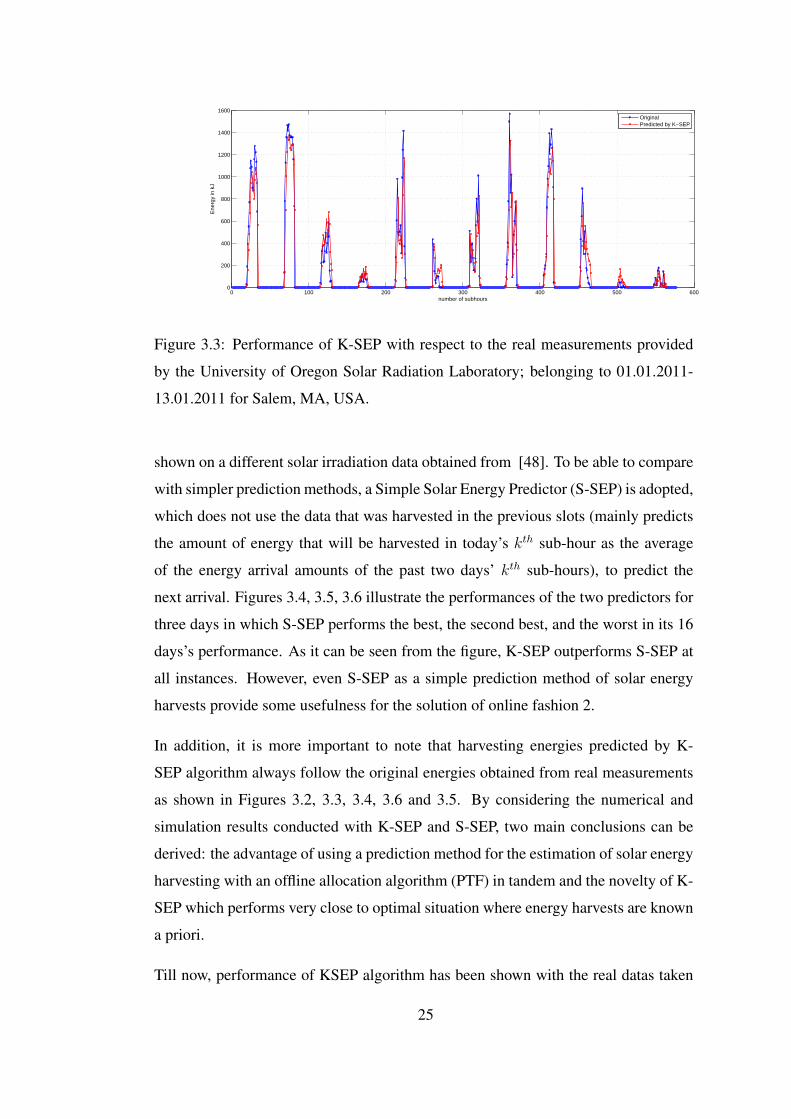
Till now, performance of KSEP algorithm has been shown with the real datas taken

25

1

0 5 10 15 20 25 30 35 40 45 500

10

20

30

40

50

60

70

OriginalPredicted by K−SEPPredicted by S−SEP

No. of sub-hours

Ene

rgy

(kilo

joul

es)

Figure 3.4: Performances of K-SEP and S-SEP compared with the real power mea-

surements provided in [48]; belonging to 16.10.2009 for Amherst, MA, USA [16].

1

0 5 10 15 20 25 30 35 40 45 500

5

10

15

20

25

30

OriginalPredicted by K−SEPPredicted by S−SEP

No. of sub-hours

Ene

rgy

(kilo

joul

es)

Figure 3.5: Performances of K-SEP and S-SEP compared with the real power mea-

surements provided in [48]; belonging to 10.10.2009 for Amherst, MA, USA [16].

26

1

0 5 10 15 20 25 30 35 40 45 500

10

20

30

40

50

60

70

OriginalPredicted by K−SEPPredicted by S−SEP

No. of sub-hours

Ene

rgy

(kilo

joul

es)

Figure 3.6: Performances of K-SEP and S-SEP compared with the real power mea-

surements provided in [48]; belonging to 04.10.2009 for Amherst, MA, USA [16].

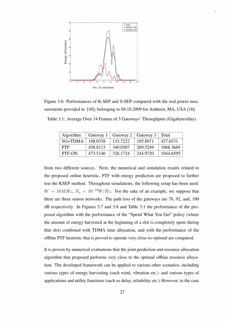
Table 3.1: Average Over 14 Frames of 3 Gateways’ Throughputs (Gigabytes/day)

Algorithm Gateway 1 Gateway 2 Gateway 3 TotalSG+TDMA 188.0338 133.7222 105.8971 427.6531PTF 458.8113 340.0307 269.5249 1068.3669PTF-ON 473.5146 326.1724 244.9720 1044.6595

from two different sources. Next, the numerical and simulation results related to

the proposed online heuristic, PTF with energy prediction are proposed to further

test the KSEP method. Throughout simulations, the following setup has been used:

W = 10MHz, No = 10−19W/Hz. For the sake of an example, we suppose that

there are three sensor networks. The path loss of the gateways are 78, 92, and, 100

dB respectively. In Figures 3.7 and 3.8 and Table 3.1 the performance of the pro-

posed algorithm with the performance of the “Spend What You Get” policy (where

the amount of energy harvested at the beginning of a slot is completely spent during

that slot) combined with TDMA time allocation, and with the performance of the

offline PTF heuristic that is proved to operate very close-to-optimal are compared.

It is proven by numerical evaluations that the joint prediction and resource allocation

algorithm that proposed performs very close to the optimal offline resource alloca-

tion. The developed framework can be applied to various other scenarios, including

various types of energy harvesting (such wind, vibration etc.) and various types of

applications and utility functions (such as delay, reliability etc.) However, in the case

27

0 2 4 6 8 10 12 140

1

2

3

4

5

No of frames

Util

ity im

p.(%

)

0 2 4 6 8 10 12 140

50

100

150

200

250

No of framesThr

ough

put i

mp.

(%)

PTFPTF−ON

PTFPTF−ON

Figure 3.7: Utility and Throughput Improvements of PTF and PTF-On over

SG+TDMA on Amherst, MA solar irradiation data.

0 2 4 6 8 10 12 140

500

1000

1500

No of frames

Tot

al th

roug

hput

(G

igab

ytes

)

ptfptfonsg+tdma

Figure 3.8: Total Throughput of the three gateways (in Gigabytes) over 14 Frames on

Amherst, MA solar irradiation data.

28

of mobile APs with unpredictable and random energy arrivals, a promising resource

allocation algorithm calls for a dynamic and stochastic policy. In the next chapters,

dynamic problem of expected utility maximization will be investigated to address this

problem.

29

30

CHAPTER 4

FINITE HORIZON DYNAMIC EXPECTED UTILITY

MAXIMIZATION UNDER ENERGY CONSTRAINTS

4.1 System Model and Problem Statement

4.1.1 System Model

Consider an Access Point (AP) moving on a path to provide service to the different

users in a large geographical area. It is powered by devices capable of energy harvest-

ing, that is, renewable energy sources such as solar, wind, vibration etc. are employed

to meet the energy expenditure of the downlink communication system. Most proba-

ble source of energy will be the solar irradiation exploiting the fact that high potential

of energy harvesting and assumption of mobile outdoor system above the level of

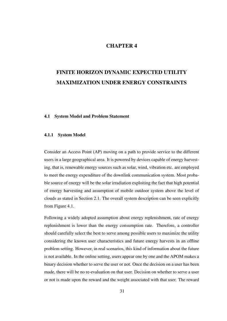
clouds as stated in Section 2.1. The overall system description can be seen explicitly

from Figure 4.1.

Following a widely adopted assumption about energy replenishment, rate of energy

replenishment is lower than the energy consumption rate. Therefore, a controller

should carefully select the best to serve among possible users to maximize the utility

considering the known user characteristics and future energy harvests in an offline

problem setting. However, in real scenarios, this kind of information about the future

is not available. In the online setting, users appear one by one and the APOM makes a

binary decision whether to serve the user or not. Once the decision on a user has been

made, there will be no re-evaluation on that user. Decision on whether to serve a user

or not is made upon the reward and the weight associated with that user. The reward

31

AP AP AP

n = 1at n = 5at n = 9at

harvester

Energy

Users (v1, w1) (v2, w2) (vN , wN )(vn, wn)

Figure 4.1: Overall system model of APOM with renewable energy sources

could be the utility of providing service to that user, and the cost may be related to

the power required to serve this user. If there was no energy limitation at the AP, it

would serve all available users to achieve maximum utility. However, when energy

replenishment rate is slower than power it would require to serve all users, the APOM

has to refuse a number of users.

Hence the problem is an online decision problem with the goal of picking a set of

users to maximize the total utility under the energy constraints regarding the causality

of this energy, and the causality of the information gathered about users.

A dynamic scenario is considered where users associated with random values and

weights appear to the APOM sequentially during its route. The characteristics of the

users (value and weight) are not known deterministically, but they become known

to the agent following the related probability distributions. The value of a user can

be defined as the instantaneous utility gained by providing service to that user. The

weight may also be related to required energy consumption of a user. Associated

value and weight distributions depend both on the requirements of a user and the

channel gain between the APOM and the user (when the user has a poor link to the

APOM, for example, the cost of serving it will be high or changes in variations of the

link quality may result in a higher variance in the rate that can be provided to it).

A (finite) sequence of users σ = 1, ..., N appearing on the APOM’s route to be pro-

32

vided with service is defined. In this simplified model, one user is observed per time

slot, which corresponds to a problem horizon of N slots. Each user arrives randomly

according to a probability distribution and is identified by a utility achieved by serv-

ing it (i.e. amount of transmitted data), and the energy consumption it requires. For

each user n, APOM chooses whether to transmit to it or not based on that user’s indi-

vidual characteristics and the probability of future possible users and energy harvests.

In the rest, each user will be classified by a "value" and "weight" pair: (vi, wi) for the

ith user, where the value corresponds to the utility gained by serving this user, and the

weight corresponds to the power consumption required to serve it. The user character-

istics are not available to the APOM in advance but become known in time of arrival,

so the (vi, wi) information of the ith user appears at the time it sends a request. The

users that APOM encounters are classified as regards their utilization vi value which

is a random variable

A finite number of discrete states for energy requirement, instantaneous utility and

energy harvesting will be assumed, which are not fully unrealistic considering some

practical correspondents to these limitations exist: in practice, APs admit only users

in a certain area of coverage, which automatically limits the power consumption.

Rewards from a user (rate, pricing, etc.) are inherently bounded. Finally, solar irradi-

ation is quite stationary on an hourly basis [49].

In the dynamic and stochastic version of the knapsack problem items arrive sequen-

tially over time and their value/weight combinations are stochastic but become known

to the scheduler at arrival times. An instantaneous decision needs to be made on each

impatient user’s arrival. The decisions are irreversible, that is, users can not be re-

called later. Once a user is rejected, value associated with that user will be lost.

Following knapsack terminology, the AP is characterized by its "capacity" to serve,

which corresponds in our case to the amount of energy it has stored in its battery.

The problem is to collect the expected reward over N users while ensuring that the

total weight does not exceed the service capacity. Stated this way, the problem is

dynamic stochastic knapsack problem as in Section 2.2. However, in accordance

with energy harvesting, capacity replenishment is allowed. At the beginning of the

problem horizon, there is a certain amount of energy, assumed to be stored in the

33

battery of the AP.

Indeed, it never makes sense to allocate an insufficient resource to a user, because

individually rational user will provide zero utility is its resource requirement not fully

be satisfied. On the other hand, allocating more energy capacity than the reported

demand is useless as well since such allocations do not further increase utility gained

more than the requested value.

Using this setup, the problem can be stated in terms of xn’s xn = {0, 1}, which

indicate the decision to either serve user n or pass it up. In terms of horizon over

which the APOM will act; the problem statement approach can be classified into two

parts: finite and infinite time horizons.

4.1.2 Problem Statement: Finite Horizon

The problem in finite horizon is to collect the expected reward (utility) over N slots

while ensuring that the total weight (energy consumption) does not exceed the en-

ergy capacity considering the random user characteristics and energy harvests in a

certain time horizon. If the problem were defined with conventional energy sources

rather than renewable energy sources, the problem formulation given in Problem 3

is a generalization of dynamic stochastic knapsack problem where the objective in

maximizing expected value.

Problem 3.

Maximize: E(N∑n=1

vnxn) (4.1)

subject to:N∑n=1

wnxn ≤ B, (4.2)

xn ∈ {0, 1} (4.3)

Then, considering the energy replenishments, available energy is the newly harvested

energy plus the energy left over from previous intervals. Energy expenditure in an

interval cannot exceed this amount. The overall structure may be modelled as an

extension of the stochastic knapsack problem with increasing capacity due to energy

34

harvests prevailing at Nk intervals as stated in Problem 4. The energy arrivals Bk’s

are modelled as IID random processes to appear at the beginning of each time slot

where Bi ∈ 0, e. Thus, energy is replenished with probability q at each interval such

as right after the N th1 slot, the N th

2 slot, and so on, up to some Nk = N .

Problem 4.

Maximize: E(

Nk∑n=1

vnxn) (4.4)

subject to:N1∑n=1

wnxn ≤ B1,

N2∑n=1

wnxn ≤ B1 +B2, ...,

Nk∑n=1

wnxn ≤k∑j=1

Bj (4.5)

xn ∈ {0, 1} (4.6)

Equations (4.4) and (4.5) indicates the objective of the problem, which is to maximize

the expected total value in a finite time horizon N under the constraints of energy

consumption. (4.5) holds for energy causality, i.e., the energy expenditure in any

interval can not be bigger than the energy production in that interval. In here, the

setup of the problem differs from the most usual knapsack problems. The assumption

that only one user can get service at each slot without preemption is given in (4.6).

Theorem 1. The utility maximization problem in energy harvesting AP stated in

Problem 4 is at least NP-hard.

Proof. The claim can be shown by a reduction from a well known NP-hard problem:

0/1 knapsack problem where proposed utilities and energy consumption demand of

each user corresponds to values and the weights of items in the knapsack. A special

case of Problem 4 is equivalent to the 0/1 knapsack problem where there are no energy

harvest or the energy harvest interval is infinitely long. The simpler version of the

Problem 4 can be stated in a same way of Problem 3 which is known to be NP-hard

[34]. Therefore Problem 4 is at least an NP-hard problem.

Following Theorem 1 and motivated by the results obtained in similar works, dy-

namic programming method offers an optimal solution to the the dynamic problem in

pseudo-polynomial time.

35

4.2 Optimal Online Solution with Dynamic Programming

Instantaneous requests are accepted by the APOM along its path as it encounters

different users. A decision has to be made as the APOM encounters a new user.

Using a threshold based approach as a decision mechanism is desirable in terms of

computational complexity. Hence, we shall mainly develop a threshold based scheme

after the optimal solution for the APOM scenario is derived via stochastic dynamic

programming.

As stated in Section 4.1.2, there are K types of users based on the utility they provide

such as vn(k) ∈ {vn(1), vn(2)} for a two user type system where users appear with

the corresponding statistics P (vi(1)) and P (vn(2)) at each slot. The costs of the users

to system wn(k)’s are considered to be all equal to w without loss of all generality.

If a user of type k appears at any slot n, then a value of v(k) and weight of w(k)

are obtained. For the following analysis, a state for the nth user is to be defined in

terms of the available energy e and user type k. Each user class denoted by k appears

as an IID process with probability p(k) such that∑K

k=1 p(k) = 1. V (e, k, n) state

denotes the expected total value from slot n till the end of time horizon N , that is,

V (e, k, n) = E(∑N

i=n vixi).

At first, future harvests are not taken into account where B1 = E is the initial amount

of energy which is also the available sack capacity. Let the action taken for nth user

be dn = {T,D} where T denotes xn = 1 and D implies that xn = 0. The action

space for N slots is denoted with the following set: d = [d1, ..., dN ]. The maximum

expected total value at slot n till the deadlineV ∗(e, k, n) can be formulated using the

dynamic programming equation as follows:

V ∗(e, k, n) = maxd{Vd(e, k, n)}, n ≥ 1, where (4.7)

Vdn(e, k, n) = v(k)xn +K∑k′=1

p(k′)V ∗(e− w(k)xn, k′, n+ 1) (4.8)

A threshold based approach is revealed after the backward induction of the dynamic

programming equation revealed that for smaller utility type users, call v(1), the func-

36

tion adopts a conservative attitude at first and turns to a Greedy form as it gets closer

to the end of the horizon,N . Whilst, the threshold function for a user type with higher

utility, of value v(2), always has a priority. The APOM attempts to serve user with

higher utility as long as the energy constraints are satisfied, which implies that the

residual energy of the APOM should be greater than the weight of the corresponding

user.

As an extension to (4.7), the energy replenishment statistics are considered where

energy arrivals may occur with probability q at each slot while incrementing the ca-

pacity by 0 or 1 since Bn ∈ {0, 1}. In the next, lets denote the harvest process with

a random variable Q which is equal to 1 with probability q and e = [1, ..., E] im-

plies the available energy at any time slot. Then, we define π as the decision policy

for a horizon that spans N slots. At each slot; a decision of Transmit or Deny is

made according to the comparison of the instantaneous reward gained by serving the

current user with the total expected reward by saving that energy for the next slots.

A Stochastic Dynamic Programming Solution using ’divide and conquer’ method is

proposed. Action dn = {T,D} corresponding xn = {1, 0}, an action space for N

slots till the end of tie horizon is denoted with the following set: d = [d1, ..., dN ]. Us-

ing Bellman’s equation for the expected value maximization dynamic programming

equation is constructed as:

V ∗(e, k, n) = maxd{Vd(e, k, n)} (4.9)

d ∈ {T,D}N (4.10)

The problem formulation using a dynamic programming equation is constructed as

follows: Start with

V ∗(e, k,N) = v(k), ∀e ≥ 1 (4.11)

and go backwards using

37

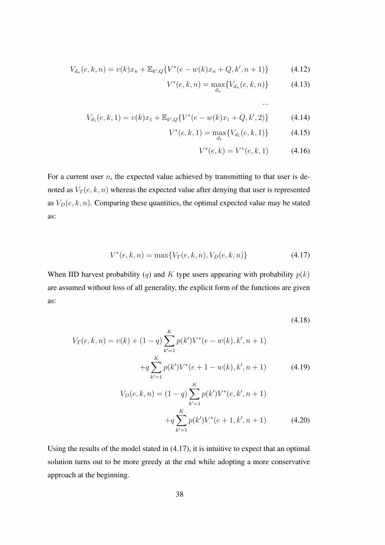
Vdn(e, k, n) = v(k)xn + Ek′,Q{V ∗(e− w(k)xn +Q, k′, n+ 1)} (4.12)

V ∗(e, k, n) = maxdn{Vdn(e, k, n)} (4.13)

...

Vd1(e, k, 1) = v(k)x1 + Ek′,Q{V ∗(e− w(k)x1 +Q, k′, 2)} (4.14)

V ∗(e, k, 1) = maxd1{Vd1(e, k, 1)} (4.15)

V ∗(e, k) = V ∗(e, k, 1) (4.16)

For a current user n, the expected value achieved by transmitting to that user is de-

noted as VT (e, k, n) whereas the expected value after denying that user is represented

as VD(e, k, n). Comparing these quantities, the optimal expected value may be stated

as:

V ∗(e, k, n) = max{VT (e, k, n), VD(e, k, n)} (4.17)

When IID harvest probability (q) and K type users appearing with probability p(k)

are assumed without loss of all generality, the explicit form of the functions are given

as:

(4.18)

VT (e, k, n) = v(k) + (1− q)K∑k′=1

p(k′)V ∗(e− w(k), k′, n+ 1)

+qK∑k′=1

p(k′)V ∗(e+ 1− w(k), k′, n+ 1) (4.19)

VD(e, k, n) = (1− q)K∑k′=1

p(k′)V ∗(e, k′, n+ 1)

+qK∑k′=1

p(k′)V ∗(e+ 1, k′, n+ 1) (4.20)

Using the results of the model stated in (4.17), it is intuitive to expect that an optimal

solution turns out to be more greedy at the end while adopting a more conservative

approach at the beginning.

38

To define DP relaxation of the problem explicitly, the pseudo code of solution is given

as follows:

Algorithm 1 DP solution to the problem for finite horizonfor e = 0toE do

for k = 1toK do

V (e, k,N + 1) = 0 {Initialization step}

end for

end for

for n = Nto1 do

for e = 0toE do

for k = 1toK do

if w(k) > e then

V (e, k, n) = E(k′,Q){V ∗(e+Q, k′, n+ 1)}else

V (e, k, n) = max{E(k′,Q){V ∗(e+Q, k′, n+ 1)}, v(k) + E(k′,Q){V ∗(e−w(k) +Q, k′, n+ 1}} {Recursive equation}

end if

return V (e, k, n)

end for

end for

end for

Theorem 2. The dynamic programming approach provides an optimal solution to

the problem defined in Section 4.1.2, where the objective function is expected utility

maximization with energy harvesting.

Proof. As a principle of DP, the problem is divided into subproblems. Moreover,

Bellman’s optimality condition states that optimization of the future does not de-

pend on the decisions in the past. Therefore, solutions in each instance is optimal

for a subproblem since the decision ({D,T}) is made according to V ∗(e, k, n) =

max{VT (e, k, n), VD(e, k, n)}. Once the decisions in each sub-problem is optimal,

Theorem can be proved by induction by following the principle of optimality defined

by Bertsekas [8].

39

4.3 Structure of the Optimal Policy

After exhibiting the stochastic dynamic programming solution, structure of the opti-

mal policy may be obtained based on the DP relaxation.

Given any finite time horizon N , intuitively, dynamic programming optimal solution

behaves more conservatively at the beginning, on the other hand, as the end of horizon

gets closer, it becomes a greedy policy. It is also intuitive to expect that an optimal

policy becomes more lenient in deciding to serve a given user as the available energy

increases and vice versa.

Theorem 3. For the dynamic stochastic Knapsack problem with increasing capacity

on a probabilistic model, the optimal online policy that maximizes the total expected

reward is of the form:

xn(k) =

1 : vn(k) ≥ β

0 : vn(k) < β(4.21)

where

β , E(k′,Q){V ∗(e+Q, k′, n+ 1)} − E(k′,Q){V ∗(e− wn(k) +Q, k′, n+ 1)}(4.22)

Proof. A valid policy makes a decision to either serve or not to serve a user at each

slot. Dynamic programming formulation implies that arg max{vn(k)+E(k′,Q){V ∗(e−wn(k)+Q, k′, n+1)},E(k′,Q){V ∗(e+Q, k′, n+1)}. V (e−wn, k, n+1) is the expected

future cost when the user is transmitted whereas V (e, k, n + 1) denotes the expected

future cost when the decision is ’Deny’. Considering Bellman’s principle of opti-

mality, the optimal policy makes a decision based on a comparison of the value that

current users offering exchange of a capacity consumption with the expected value

that can be obtained with this energy expenditure in the remaining slots to maximize

the total expected utility.

The result of Theorem 3 may be considered to be straightforward to show regard to

DP relaxation. However, structural properties of the optimal solution and whether

40

there exists a threshold based policy on the available energy depending on problem

state need to be examined in detail.

4.3.1 Existence of Threshold

Lemma 1. For a given k and n, the state defined as expected total reward V (e, k, n)

is super-modular in available energy and decision pair (e,d), that is VT (e+ 1, k, n) +

VD(e, k, n) ≥ VD(e+ 1, k, n) + VT (e, k, n) where 1 ≤ n ≤ N and d ∈ {T,D}.

Proof. Stated super-modularity corresponds the statement:

VT (e+ 1, k, n)− VD(e+ 1, k, n) ≥ VT (e, k, n)− VD(e, k, n), 1 ≤ n ≤ N (4.23)

which can be shown to hold by the following argument:

VT (e, k, n)− VD(e, k, n) = v(k) +K∑k′

qV (e, k′, n+ 1) + (1− q)V (e− 1, k′, n+ 1)

−K∑k′

qV (e+ 1, k′, n+ 1) + (1− q)V (e, k′, n+ 1)

(4.24)

= v(k) +K∑k′=1

q(V (e, k′, n+ 1)− V (e+ 1, k′, n+ 1))

+(1− q)(V (e− 1, k′, n+ 1)− V (e, k′, n+ 1))

(4.25)

and,

VT (e+ 1, k, n)− VD(e+ 1, k, n) = v(k) +K∑k′=1

q(V (e+ 1, k′, n+ 1)− V (e+ 2, k′, n+ 1))

+(1− q)(V (e, k′, n+ 1)− V (e+ 1, k′, n+ 1))

(4.26)

By subtracting (4.25) from (4.26), a sufficient condition for (4.23) to hold becomes:

V (e, k, n)− V (e− 1, k, n) ≥ V (e+ 1, k, n)− V (e, k, n) (4.27)

∀n ≥ 1

41

Then, the condition of (4.27) is proved by induction. First, the condition is satisfied

when n = 1, that is both sides of the equation are equal to 0. Second, if it is true for

some n− 1 then it also holds for n.

V (e, k, n)− V (e− 1, k, n) ≥ V (e+ 1, k, n)− V (e, k, n) (4.28)

We will examine the three cases corresponding 3 energy states (e + 1, e, e − 1) and

the three decisions (d1, d2, d3 ∈ {T,D}) respectively.

Vd1(e+ 1, k, n)− Vd2(e, k, n)− (Vd2(e, k, n)− Vd3(e− 1, k, n)) ≤ 0 (4.29)

Vd1(e+ 1, k, n)− Vd1(e, k, n) + Vd1(e, k, n)− Vd2(e, k, n)

−(Vd2(e, k, n)− Vd3(e− 1, k, n))− Vd3(e, k, n) + Vd3(e, k, n) ≤ 0 (4.30)

By optimality of d2 for energy state e, Vd1(e, k, n)− Vd2(e, k, n) statement is already

smaller and equal to 0. Same property holds for the Vd3(e, k, n) − Vd2(e, k, n) state-

ment. Therefore, we should only consider the remaining terms. For each possible

cases of [d1, d3] ∈ {T,D}2, the inequality in (4.30) is shown to be satisfied. For

example, lets examine the case where d1 = T and d2 = T :

VT (e+ 1, k, n)− VT (e, k, n)− (VT (e, k, n)− VT (e− 1, k, n))

=K∑k′=1

p(k)q(V (e+ 1, k, n− 1)− V (e, k, n− 1)

−V (e, k, n− 1) + V (e− 1, k, n− 1))

+(1− q)(V (e, k, n− 1)− V (e− 1, k, n− 1)

−V (e− 1, k, n− 1) + V (e− 2, k, n− 1)) ≤ 0 (4.31)

The above inequality holds since the difference is assumed to be non increasing in

e. Similar steps may be followed for all combinations of d1 and d3 where [d1, d3] ∈{T,D}2. Hence, the total expected reward is a super-modular function in (d,e).

Lemma 2. Suppose decision is ′T ′ when state is (e1, k, n), then the decision is ′T ′ for

the state (e2, k, n) for all e2 ≥ e1 such that {e1, e2} ∈ E2.

Proof. Following Lemma 1 namely the super-modularity property, it can be stated

that:

VT (e+ 1, k, n)− VD(e+ 1, k, n) ≥ VT (e, k, n)− VD(e, k, n) (4.32)

42

when the optimal decision is ′T ′ for a state (e, k, n), by Bellman’s equation:

VT (e, k, n) ≥ VD(e, k, n) (4.33)

then, combining (4.32) with (4.33), we have:

VT (e+ 1, k, n) ≥ VD(e+ 1, k, n) (4.34)

as a result, optimal solution is ′T ′ for the energy state e+ 1 if it is ′T ′ for state e, that

is, if d(e) = T then d(e+ 1) = T .

Theorem 4. The optimal policy is a threshold type policy in the available energy at

each slot n and there is a threshold η defined as: xn(k) =

1 : e ≥ η(n, k)

0 : e < η(n, k)

Proof. Let {e1, e2, e3} be the available energies at three decision instants such that

e1 < e2 < e3. For the sake of reaching contradiction, let’s assume that the optimal

policy is not a threshold based policy. Then, there exists an optimal policy which

chooses to ′T ′ at energy levels e1 and e3 while denying the user at the energy level

e2. This contradicts with Lemma 2; hence, the assumed policy was not optimal.

Therefore, the crossover from ′D′ to ′T ′ happens only one as e is increased (holding

all other parameters constant). This implies the existence of threshold.

4.3.2 Monotonicity of Threshold

First, the following obvious result is recorded.

Proposition 1. When users k = 1, 2, ..., K with identical resource demands w(k)’s

are given such that v(1) ≤ v(2) ≤ ... ≤ v(K), then V (e, k, n) ≤ V (e, k + 1, n) .

Proof. Since V (e, k, n) = max{v(k)+V (e−w(k), n+1), V (e, n+1)} and V (e, k−1, n) = max{v(k − 1) + V (e − w(k − 1), k, n + 1), V (e, k, n + 1)}, the RHS of

two equations differ only in the first terms inside the bracket. Considering v(k) ≤v(k + 1), the statement in the proposition is shown to hold.

Proposition 2. V (e, k) is a non-decreasing function of e.

43

Proof. Proof follows by inspection of the value function in 4.2.

Lemma 3. Expected total reward ′V (e, k, n)′ is super-modular in slot number and

decision pair (n,d), that is VT (e, k, n+1)+VD(e, k, n) ≥ VD(e, k, n+1)+VT (e, k, n).

Proof. Following the similar steps in the proof of lemma 1, supermodularity corre-

sponds to the statement:

VT (e, k, n+ 1)− VD(e, k, n+ 1) ≥ VT (e, k, n)− VD(e, k, n) (4.35)

VT (e, k, n+ 1)− VD(e, k, n+ 1) = v(k)+

K∑k′=1

q(V (e, k′, n+ 2)− V (e+ 1, k′, n+ 2))

+(1− q)(V (e− 1, k′, n+ 2)− V (e, k′, n+ 2)) (4.36)

VT (e, k, n)− VD(e, k, n) = v(k)+

K∑k′=1

q(V (e, k′, n+ 1)− V (e+ 1, k′, n+ 1))

+(1− q)(V (e− 1, k′, n+ 1)− V (e, k′, n+ 1)) (4.37)

(4.38)

by subtracting (4.36) from (4.37), the condition becomes:

V (e− 1, k, n+ 1)− V (e, k, n+ 1) ≤ V (e− 1, k, n+ 2)− V (e, k, n+ 2) (4.39)

which is equivalent to:

V (e, k, n+ 1)− V (e, k, n+ 2) ≥ V (e− 1, k, n+ 1)− V (e− 1, k, n+ 2) (4.40)

Expected total value is a non-increasing function of slot-number (both sides of the in-

equality have nonnegative values) and a non-decreasing function of available energy,

therefore inequality in (4.40) holds for all e, k, n variables.

Lemma 4. Suppose decision is ′T ′ when state is (e, k, n), then the decision is ′T ′ for

the state (e, k, n+ 1) for all n such that n ∈ {1, ..., N}.

Proof. Lemma holds when the state defined as expected total reward ′V (e, k, n)′ is

super-modular in (n,x), that is VT (e, k, n + 1) + VD(e, k, n) ≥ VD(e, k, n + 1) +

44

VT (e, k, n). When super-modularity holds: VT (e, k, n + 1) − VD(e, k, n + 1) ≥VT (e, k, n) − VD(e, k, n). Thus, considering the Bellman’s decision formulation it

is straightforward that the decision is ′T ′ for the state (e, k, n + 1) if it is ′T ′ when

state is (e, k, n).

Theorem 5. The threshold function on the available energy to serve a user, η(n, k)

defined in Theorem 4 is monotonically non-increasing with slot number n. Moreover,

the threshold function on the users’ value, β(e, n) defined in (4.22) is monotonically

non-increasing with slot number n and monotonically non-decreasing with energy

level e.

Proof. The proof follows the Lemma 4. Theorem may further be proved by contra-

diction. Let {n, n + 1} be the available slot numbers such that n ≥ 1. Let’s assume

that the optimal threshold value is increasing with slot number. Then, there exists

an optimal policy which chooses to transmit at slot n while denying a user of type k

at the slot n + 1. Following the formulation given in Theorem 3 results of Lemmas

3 and 4, it is feasible but not a solution of the Bellman equation. Therefore a valid

threshold function is monotonically non-increasing with slot number n. Monotonic-

ity with respect to energy level e can be shown following the similar steps stated for

slot number n.

4.3.3 Curse of dimensionality

Dynamic programming method provides an optimal solution for 0/1 dynamic and

stochastic resource allocation problem with randomly growing capacity; however as

in most optimization problems it suffers from ’curse of dimensionality’. Indeed, the

result is consistent with the NP-hardness definition such that there is no algorithm

that works both optimal and fast.

Both computational and storage requirements grow exponentially as the number of

state and control variables increases. The control variables in this problem have only

two states {T,D}, but the state variables quickly explode with increasing number of

possible user types (K), energy states (E) and length of time horizon (N ). Its com-

putational complexity is O(2(NEK)) which might cause low performance and unnec-

45

essary delays in practical situations with high dimension. In the next, some methods

and heuristics will be proposed to deal with this ’curse of dimensionality’.

4.4 Suboptimal Solution: Expected Threshold Policy

The curse of dimensionality may be overcomed by using pre-calculated tables that

include optimal expected values and the decision might be done upon them. How-

ever, it still needs a high amount of memory by exchanging time complexity with

space complexity. Moreover, in real life scenarios with dynamically changing envi-

ronment, this is not feasible. To deal with the cases where real time computation is

necessary; some suboptimal approaches with low complexity is needed. In this sec-

tion, a computationally cost effective suboptimal policy called "Expected Threshold"

is derived.

Considering the structure of optimal online policy, decision of transmitting to a user

or not is made mostly upon the available energy on that time. In the computationally

cost effective suboptimal solution approach, we set some energy boundaries on each

user type that AP should have in order to serve that user. In the process of constituting

an energy threshold, AP should also regard the potential energy harvests till the end

and potential user characteristics.

Each user class denoted by k appears as an IID process with probability p(k) such that∑Kk=1 p(k) = 1. V (e, k, n) state denotes the expected total value from slot n till the

end of time horizon N . Considering the causality constraint on energy, the amount of

depleted energy in any interval can not be bigger than the sum of available energy at

the beginning of that interval plus the energy renewed, we define the following bound

on the expectation of energy depletion (RHS of (4.41)) at slot n if the energy is e and

expected harvest amount from slot n till the end of time horizon N if is denoted asN−1∑m=n

E{Qm|Qn−11 } .

e+N−1∑m=n

E{Qm|Qn−11 } ≥

N∑m=n+1

E{wmxm} (4.41)

46

If the weights are all equal and harvest process is IID then, the inequality 4.41 be-

comes:

e+

(N−1)∑m=n

q ≥ (N − n+ 1)w (4.42)

After stating a bound of the expected energy consumption from slot n till the end

of time horizon in (4.42), a computationally cost effective suboptimal policy called

"Expected Threshold" is proposed as follows in (4.43):

xn(k) =

1 : e ≥ η

0 : e < η(4.43)

where

η = (N − n+ 1)(K∑

k′=k+1

p′k − q) (4.44)

As it can be seen from (4.43) and (4.44, APOM makes a decision to serve a user of

type k appearing in slot n if the available energy e at slot n is greater or equal to

threshold level η. η is stated as the difference between the expected energy consump-

tion for users with higher value and expected energy replenishment from slot n till

the end of time horizon N .

It can be devised from (4.44) that threshold function follows the structure of the op-

timal policy defined in Sec. (4.3), i.e. monotonically decreases with slot number and

harvest rate depending on the probability distribution of users.

Please note that, without loss of generality, a suboptimal threshold function can be

derived for general distribution of harvest event as in (4.45) and (4.46) following the

bound in (4.41).

xn(k) =

1 : e ≥ η

0 : e < η(4.45)

47

where

η =N∑

m=n+1

E{wmxm} −N−1∑m=n

E{Qm|Qn−11 } (4.46)

To examine the performance of the expected threshold policy in the next section (4.5),

two more different heuristics are also defined as: greedy policy (Definition 1) and

conservative policy (Definition 2).

Definition 1. Greedy policy is a policy that decides to serve an appearing user when-

ever there is available energy to serve it.

Definition 2. Conservative policy is a policy that serves only the best user when there

is available energy to serve it.

4.5 Performance Evaluation and Numerical Results

It appears that an optimal policy becomes more lenient in accepting demands as the

deadline approaches, the remaining amount of resource increases; in other words, the

optimal reward threshold is decreasing in time for any given resource requirement

and increasing in the expected amount of energy incoming.

The two observations given above have been proved in previous section. The sub-

optimal policy is also shown to exhibit the same structural characteristics defined in

the section. The statement can further be justified by considering the sub-optimal

threshold function.

Adopting the suboptimal threshold policy defined in (4.43), the results are obtained

and compared with the optimal policy over 10000 Monte Carlo Simulations as illus-

trated in Figures 4.2 and 4.3 for two different levels of initial energy stored in the

battery and the two different energy harvest probabilities. It can be deduced from the

figures that, initial stored energy effect on the performance is insignificant.

It is observed that both the optimal and suboptimal policies behaves more conserva-

tively at the beginning, then as the end of horizon gets closer, it becomes a greedy

policy given any finite time horizon N . As illustrated in Figures 4.4 and 4.5, the Ex-

pected Threshold Policy is shown to perform very close to optimal policy. However

48

q=0.2 q=0.5 q=0.80

20

40

60

80

100

120

140

160

180

Harvest Probability

Exp

ecte

d To

tal V

alue

optimal by DPexpected threshold

Figure 4.2: The performance evaluation of Expected Energy Threshold Heuristic wrt.

Optimal Policy when available energy=10, N = 20, K = 2 for two different user

types with efficiency ratios 10 and 5

q=0.2 q=0.5 q=0.80

20

40

60

80

100

120

140

160

180

Harvest Probability

Exp

ecte

d To

tal V

alue

optimal by DPexpected threshold

Figure 4.3: The performance evaluation of Expected Energy Threshold Heuristic wrt.

Optimal Policy when available energy=5,N = 20,K = 2 for two different user types

with efficiency ratios 10 and 5

49

0.1 0.2 0.3 0.4 0.5 0.6 0.7 0.8 0.9 1100

200

300

400

500

600

700

800

900

Harvest Probability (q)

Expe

cted

Tol

tal V

alue

ove

r 100

Slo

ts

optimal by DPgreedyconservativeexpected threshold

Figure 4.4: The comparison of the performances for Expected Energy Threshold Pol-

icy, Greedy Policy and Conservative Policy with respect to Optimal Policy when

available energy=5, N = 100, K = 2 for two different user types with efficiency

ratios 10 and 5 (best users appearing with high probability e.g. 0.7)

the greedy and conservative policies perform less efficiently compared with the pro-

posed heuristic. It can also be derived from Figure 4.4 that when the efficient users

appear with high probability, conservative policies outperforms greedy policies. On

the other hand, when the inefficient users appear with low probability, greedy poli-

cies are more advantageous than the conservative approaches. However, Expected

Threshold Policy proposed in this thesis is robust to variations in user distributions.

In addition, to investigate more general scenarios number of user types (K) is in-

creased to 5 and simulations has been conducted on the users with both the equal

weight (energy demand) in Figure 4.6 and different weights in Figure 4.7. In Fig-

ure 4.7, simulations have been conducted for five different user types with efficiency

(value/weight) ratios given as [10/1, 5/1, 8/4, 5/8, 2/6 1/5] with probabilities [0.3 0.15

0.15 0.3 0.1]. As it can be seen from Figures 4.6 and 4.7, performance of the Expected

Threshold Policy is very close to optimal.

50

0.1 0.2 0.3 0.4 0.5 0.6 0.7 0.8 0.9 10

100

200

300

400

500

600

700

Harvest Probability (q)

Expe

cted

Tot

al V

alue

ove

r 100

Slo

ts

optimal by DPgreedyconservativeexpected threshold

Figure 4.5: The comparison of the performances for Expected Energy Threshold Pol-

icy, Greedy Policy and Conservative Policy with respect to Optimal Policy when

available energy=5, N = 100, K = 2 for two different user types with efficiency

ratios 10 and 5 (worst users appearing with high probability e.g. 0.7)

51

0.1 0.2 0.3 0.4 0.5 0.6 0.7 0.8 0.9 150

100

150

200

250

300

350

400

450

500

Harvest Probability (q)

Exp

ecte

d To

tal V

alue

ove

r 100

slo

ts

optimal by DP greedyconservativeexpected threshold

Figure 4.6: The comparison of the performances for Expected Energy Threshold

Policy, Greedy Policy and Conservative Policy with respect to Optimal Policy when

available energy=5 at the beginning, N = 100, K = 5 for five different user types

with equal weights

0.1 0.2 0.3 0.4 0.5 0.6 0.7 0.8 0.9 10

50

100

150

200

250

300

Harvest Probability (q)

Exp

ecte

d To

tal V

alue

ove

r 100

slo

ts

optimal by DPgreedyconservativeexpected threshold

Figure 4.7: The comparison of the performances for Expected Energy Threshold

Policy, Greedy Policy and Conservative Policy with respect to Optimal Policy when

available energy=5 at the beginning, N = 100, K = 5 for five different user types

with different efficiency (value/weight) ratios and different weights

52

CHAPTER 5

INFINITE HORIZON DYNAMIC EXPECTED UTILITY

MAXIMIZATION UNDER ENERGY CONSTRAINTS

5.1 System Model and Problem Statement

When we would like to look infinitely far into the future, we need to maximize the

total expected reward not only in a bounded time horizon, but also the expected total

reward in an infinite time horizon. Please note that, an effective problem statement

should be assumed to satisfy convergence in infinite horizon optimal policy. Two

achieve this, one can consider the mean of expected reward infinite horizon or intro-

duce a discount factor to the problem defined in Chapter 4. In this chapter, infinite

horizon problem will be investigated with these two approaches.

5.1.1 System Model

The explicit model is given in the Figure 5.1 where a constant amount of energy

(E0) is replenished at random times (Ti). Each (Tn) interval with constant amount

of capacity is called as an ’epoch’. The user distribution in all epochs is assumed

to be same with rates λ = {λ1, λ2, ..., λK}. Again in the previous chapters, assume

that each user associated with a instantaneous utility (vn) and energy demand (wn) is

appearing sequentially and request service.

Following a widely adopted assumption about stochastic energy replenishment mod-

elling [58], the harvest rate is assumed as a Poisson process with exponential inter-

arrival times Tn. The goal is to maximize the expected utility while regarding the

53

E0 E0 E0 E0 E0 E0

T1 T2 T3 T4

User

requests

Energy

harvests

Figure 5.1: The overall system model for APOM with random energy harvesting

intervals

energy arrival and user arrival statistics.

5.1.2 Problem Statement of Maximizing Mean Reward

The statement of the mean expected utility maximization problem over infinite epochs

is stated in 5.

Problem 5.

Maximize: limN→∞

1

N

N∑n=1

E{Vn} (5.1)

subject to: limN→∞

1

N

N∑n=1

E{Wn} ≤ E0 (5.2)

where

Vn =Tn∑i=1

vixi (5.3)

Wn =Tn∑i=1

wixi (5.4)

∀n ∈ 1, ..., N as N →∞ (5.5)

In (5.1), the mean of expected values in each epoch (n)is tried to be maximized where

Vn stands for the sum of values obtained from selected items in that epoch. (5.1) rep-

resents the energy limitation based on the energy replenishment rate. Wn denotes the

sum of energy consumption of selected users and (5.4) stands for the energy causality

constraint between replenishments.

54

5.1.3 Problem Statement of Maximizing Discounted Expected Reward

When one would like to look infinitely far into the future, one will try to maximize

the total expected reward not only in a bounded time horizon, but also the expected

discounted reward in an infinite time horizon.

Here, we need to introduce a discount factor γ, to state the fundamental intuition in

many areas such as economics, machine learning, operations research: "Money today

is worth more than money tomorrow". If we do not have a discount factor for the

future rewards, the obvious behaviour of the optimal algorithm in infinite horizon will

be to wait for the user with highest value since we do not have any delay constraints

here. Please note that, the infinite horizon optimal policy is stationary, i.e. optimal

decision at a state s is the same decision at all times.

Problem 6.

Maximize: E{ limN→∞

N∑n=1

γnvnxn} (5.6)

subject to:N1∑n=1

wnxn ≤ B1, (5.7)

N2∑i=1

wnxn ≤ B1 +B2, ..., limN→∞

N∑i=1

wnxn ≤ limM→∞

M∑j=1

Bj (5.8)

xi ∈ {0, 1} (5.9)

Despite the fact that the expectation is computed over an infinite sum, it is guaranteed

to converge since value is defined over a finite state space, and γ ∈ (0, 1).

5.2 Optimal Online Solution with Dynamic Programming

5.2.1 Markov Decision Process

In the previous sections, we have analysed the APOM resource allocation problem as

a stochastic knapsack problem in infinite horizon. Next, we will propose a Markov

Decision Model (MDP) to APOM resource allocation problem in infinite horizon with

discounted reward.

55

To define a MDP, the problem statement may be written explicitly as follows: For a

given set of states S and a set of decisions ′D′, ′T ′ denotes the transition probabilities

and R is the reward at each slot. State s is defined as the available energy e at the

current slot. The reward function, R and the transition probability matrix, T depend

on the harvest and user characteristics. T matrix represent the probability of next state

s’ if the current state is s and action d is taken. The instantaneous reward, R is equal

to utility provided by that user if the decision is to serve and it is zero if the decision is

not to serve. The main goal is to maximize the expected sum of discounted rewards.

V ∗(s) = maxd

∑s′

T (s, d, s′)[R(s, d, s′) + γV ∗(s′)] (5.10)

V ∗ is an optimal value function computed over the discounted infinite horizon which

satisfies Bellman equations. The MDP may be solved with value or policy iteration

policies. Iteration continues until the value function converges. Hence, following

the assumption ‖V ∗(e, k, n) − V ∗(e, k, n + 1)‖ ≤ ε where ε � 1, we may state

V ∗(e, k) = V ∗(e, k, n) for all n for infinite discounted problem statement.

The pseudo code based on DP method that summarizes the value iteration for the cal-

culation of expected optimal value and the related policy are stated as the following.

Algorithm 2 Value iteration for infinite horizonfor each state (e,k) do

while ‖V ∗(e, k, n)− V ∗(e, k, n+ 1)‖ ≤ ε do

for each state (e,k) do

if w(n) > e then

V ∗(e, k) = γE(k′,Q){V ∗(e, k′)}else

V ∗(e, k) = max{γE(k′,Q){V ∗(e, k′)}, v(k) + γE(k′,Q){V ∗(e −w(k), k′)}}

end if

end for

end while

end for

56

5.3 Suboptimal Online Policy

Again the optimal solution suffers from the "curse of dimensionality" growth of the

state space and the fact that DP conducts a search over this space. The situation is

consistent with the NP-hardness of knapsack problems.

5.3.1 Suboptimal Online Solution: Renewal Modelling

While trying to maximize the mean value over an infinite horizon, the optimal policy

is stationary [8] if the underlying processes are stationary , i.e. the optimal action will

be taken in any epoch should be equivalent.

The average rate of energy consumption up to any time t should be smaller or equal

to average rate of replenishment. Lets denote the energy replenishment rate with P

which is actually a random variable. The causality constraint may defined as follows:

K∑k=1

µkλkw(k) ≤ P (5.11)

Assume that user types are arranged such that v(1)/w(1) ≤ v(2)/w(2) ≤ ... ≤v(K − 1)/w(K − 1) ≤ v(K)/w(K). When the acceptance rate for each user k is

denoted as µk, the suboptimal policy defined as:

µk = max{0,min{P −

∑Kk′=k+1 µk′λ

′kw(k′)

λkw(k), 1}} (5.12)

The time complexity of the randomized suboptimal policy is O(K), since the accep-

tance rate calculation is repeated for all user types.

5.3.2 Suboptimal Online Solution: L-Level Lookahead Policy

Please note that, the infinite horizon optimal policy is stationary, i.e. optimal decision

on a state s is the same decision at all times. Despite the fact that the expectation

57

is computed over an infinite sum, it is guaranteed to converge since value is defined

over a finite state space where γ ∈ (0, 1). An approximate policy can be derived by

ignoring the effects of slots after Lth slot in the future. The solution will compute

L-level DP results by reducing computational complexity to O(2L) at each decision

time.

The problem of maximizing discounted utility subject to energy constraints is intro-

duced in Section 5.1.3.

V ∗ = maxπVπ (5.13)

The discounted value obtained under policy π can be formulated as the following.

V π = E{∞∑n=1

γngn(en, k)} (5.14)

where gn(en, k) is defined as the reward obtained at time n when available energy is

en and k type users appears. (5.14) can be restated as:

V π = E{L∑n=1

γngn(en, k)}+ E{∞∑

n=L+1

γngn(en, k)} (5.15)

Proposition 3. The reward obtained at time n, gn(en, k), is upperbounded by the

reward obtained from the user with best value, i.e, vK .

Proof. Since only one users can be served in a time slot n, the reward will be equal

to values offered by a user admitted in that slot. The lemma holds because of the

assumption in the finite set of users with finite set of values.

Lemma 5. The L-level Lookahead Policy, the optimal value is approximated byγLvK1− γ

depending on the discount factor and user characteristics.

Proof. Following the Proposition 3, the discounted value of the slots after L is upper-

bounded as:

58

Table 5.1: Performance Evaluation of L-level Heuristic with Respect to OptimalBased on DP for Different Values of Discount Factor, γ

Methods γ =0.1 γ =0.3 γ =0.5 γ =0.9Optimal with DP 8.48 12.14 16.85 57.813-Level Heuristic 8.46 12.02 15.90 55..42

E{∞∑

n=L+1

γngn(en, k)} = E{∞∑

n′=L

γn′gn′(en′ , k)} (5.16)

E{∞∑

n′=L

γn′gn′(en′ , k)} ≤ γLvK

1− γ(5.17)

Therefore, in the L-level Lookahead policy, the optimal value is approximated byγLvK1− γ

depending on the discount factor and user characteristics.

The performance will also be shown through simulations in Section 5.4.

5.4 Performance Evaluation and Numerical Results

To illustrate the performance of L-level heuristic in Section 5.3.2, a simulation has

been conducted with 1000 Monte Carlo trials for 3-level heuristic case where q =

0.3, users of two type (v1 = 10 and v2 = 5) appear with probability (0.3 and 0.7)

respectively. The average over obtained results are very close DP solution as can be

seen from Table 5.1.

The results are also consistent with the approximation factor found in Section 5.3.2,

that isγLvK1− γ

.

59

60

CHAPTER 6

CONCLUSION

Throughout this thesis, the problem of dynamic user admission for an Access Point on

the Move (APOM) scenario is addressed in a stochastic manner. At first, a detailed

background on the resource allocation problems in energy harvesting wireless net-

works and on knapsack problems have been provided. Observations and performance

results related to the possible approaches to related problems have been examined.

Then, exploiting the inherent properties of renewable solar energy, a Kalman filter

based solar prediction algorithm as novel method to adopt a valid offline resource

allocation policy to online situations have been investigated.

Then, a finite-horizon dynamic utility-maximizing allocation problem with a discrete

set of user requests has been formulated as a dynamic and stochastic 0/1 knapsack

problem with randomized incremental capacity. The structure of the optimal solution

of this problem has been studied through stochastic dynamic programming relaxation.

It is proved that a threshold based policy is optimal for the problem and threshold is

monotonic with respect to both available energy and slot number, where each user is

admitted if its utility to weight ratio exceeds a certain threshold. Moreover, an effi-

cient suboptimal policy to exhibit the structural properties of the optimal policy with

low computational cost has been proposed. Experimental results demonstrate that

the proposed decision methods using different threshold policies for the stochastic

resource allocation problem of the energy harvesting Access Point on the Move are

efficient in achieving close to optimal performances.

Likewise, the problem of expected discounted utility maximization problem has been

formulated in infinite horizon. The problem is formulated as a Markov decision prob-

61

lem and solved with value iteration method. Stationary of the infinite horizon pol-

icy has been shown to hold following the idea of convergence in discounted reward.

Again, a suboptimal policy with low computational complexity has been proposed

and performance results have been analysed.

The APOM defined in this thesis is powered by renewable energy sources that have

the capability of energy harvesting in a stochastic manner, which corresponds to in-

cremental capacity. Although the results have been obtained for the dynamic user ad-

mission problem, they are also applicable to other instances of dynamic and stochastic

knapsack problems with randomized incremental capacity. The insights gained in this

study can be a basis for a more generic consideration of dynamic knapsack problems

with incremental capacity that have a lot of real life applications in operational re-

search, economics, computer science, satellite and ad-hoc networks etc.

62

REFERENCES

[1] Loon for all, May 2014.

[2] M. Ajmone Marsan and M. Meo. Green wireless networking: Three ques-tions. 2011 The 10th IFIP Annual Mediterranean Ad Hoc Networking Work-shop, pages 41–44, June 2011.

[3] B. Akgün. Duty cycle optimization in energy harvesting sensor networks withapplication to bluetooth low energy. Master’s thesis, METU, June 2014.

[4] A. Alkesh, A. Singh, and N. Purohit. A moving base station strategy using fuzzylogic for lifetime enhancement in wireless sensor network. In CommunicationSystems and Network Technologies (CSNT), 2011 International Conference on,pages 198–202, June 2011.

[5] K. Amaruchkul, W. L. Cooper, and D. Gupta. Single-leg air-cargo revenuemanagement. Transportation Science, 41(4):457–469, 2007.

[6] B. T. Bacinoglu and E. Uysal-Biyikoglu. Finite horizon online lazy schedul-ing with energy harvesting transmitters over fading channels. CoRR,abs/1312.4798, 2013.

[7] B. T. Bacinoglu and E. Uysal-Biyikoglu. Finite-horizon online transmissionrate and power adaptation on a communication link with markovian energy har-vesting. CoRR, abs/1305.4558, 2013.

[8] D. P. Bertsekas. Dynamic Programming and Optimal Control, Vol. II, 2nd Ed.Athena Scientific, Belmont, MA, 2001.

[9] R. Bogue. Solar-powered sensors: a review of products and applications. Sen-sor Review, 32(2):95–100, 2012.

[10] R. L. Carraway, R. L. Schmidt, and L. R. Weatherford. An algorithm for max-imizing target achievement in the stochastic knapsack problem with normal re-turns. Naval Research Logistics (NRL), 40(2):161–173, 1993.

[11] E. T. Ceran, T. Erkilic, E. Uysal-Biyikoglu, T. Girici, and K. Leblebicioglu.Wireless access point on the move: Dynamic knapsack with incremental ca-pacity. In Globecom 2014 - Symposium on Selected Areas in Communications:GC14 SAC Green Communication Systems and Networks (GC14 SAC GreenCommunication Systems and Networks), Austin, USA, Dec. 2014. submitted.

63

[12] J. L. Crassidis and J. L. Junkins. Optimal Estimation of Dynamic Systems.Chapman and Hall, Abingdon, 2004.

[13] B. C. Dean, M. X. Goemans, and J. Vondrák. Approximating the stochasticknapsack problem: The benefit of adaptivity. Mathematics of Operations Re-search, 33(4):945–964, 2008.

[14] B. Devillers and D. Gunduz. Energy harvesting communication system withbattery constraint and leakage. In GLOBECOM Workshops (GC Wkshps), 2011IEEE, pages 383–388, Dec 2011.

[15] T. Erkılıç. Optimizing the service policy of a mobile service provider throughcompetitive online solutions to the 0/1 knapsack problem with dynamic capac-ity. Master’s thesis, METU, June 2014.

[16] N. T. Ersoy. Efficient Resource Allocation in Energy Harvesting Wireless Net-works. PhD thesis, METU, 2013.

[17] S. Gao, H. Zhang, and S. K. Das. Efficient data collection in wireless sensornetworks with path-constrained mobile sinks. IEEE Transactions on MobileComputing, 10(4):592–608, Apr. 2011.

[18] M. R. Garey and D. S. Johnson. “ strong ” np-completeness results: Motivation,examples, and implications. J. ACM, 25(3):499–508, July 1978.

[19] B. T. B. E. U. B. Goksel Uctu, Omer Melih Gul. Implementation of energy effi-cient scheduling policies on software defined radio. In Globecom 2014 - Wire-less Networking Symposium (GC14 Wireless Networking Symposium), Austin,USA, Dec. 2014. submitted.

[20] O. M. Gul and E. U. Biyikoglu. Achieving nearly 100% throughput withoutfeedback in energy harvesting wireless networks. In ISIT 2014 – InternationalSymposium on Information Theory, Hawaii, USA, 2014. accepted.

[21] O. M. Gul and E. U. Biyikoglu. A randomized scheduling algorithm for en-ergy harvesting wireless sensor networks achieving nearly 100% throughput. InWCNC 2014 - Wireless Communication and Networking Conference, Istanbul,Turkey, Apr. 2014. pp. 2492-2497.

[22] S. Guo and Y. Yang. A distributed optimal framework for mobile data gatheringwith concurrent data uploading in wireless sensor networks. In INFOCOM,2012 Proceedings IEEE, pages 1305–1313, March 2012.

[23] X. Han, Y. Kawase, and K. Makino. Randomized algorithms for removable on-line knapsack problems. In M. Fellows, X. Tan, and B. Zhu, editors, Frontiersin Algorithmics and Algorithmic Aspects in Information and Management, vol-ume 7924 of Lecture Notes in Computer Science, pages 60–71. Springer BerlinHeidelberg, 2013.

64

[24] C. Harress. Facebook (fb) to buy solar-powered drone company that can beaminternet from the sky, 2014.

[25] M. Kashef and A. Ephremides. Optimal packet scheduling for energy harvestingsources on time varying wireless channels. Communications and Networks,Journal of, 14(2):121–129, April 2012.

[26] A. J. Kleywegt and J. D. Papastavrou. The dynamic and stochastic knapsackproblem. Oper. Res., 46(1):17–35, Jan. 1998.

[27] A. J. Kleywegt and J. D. Papastavrou. The dynamic and stochastic knapsackproblem with random sized items. Oper. Res., 49(1):26–41, Jan. 2001.

[28] C. E. Koksal and N. B. Shroff. Near Optimal Power and Rate Control of Multi-Hop Sensor Networks With Energy Replenishment: Basic Limitations WithFinite Energy and Data Storage. IEEE Transactions on Automatic Control,57(4):815–829, Apr. 2012.

[29] E. Lawler. Fast approximation algorithms for knapsack problems. In Founda-tions of Computer Science, 1977., 18th Annual Symposium on, pages 206–213,Oct 1977.

[30] W. Liang, J. Luo, and X. Xu. Prolonging network lifetime via a controlledmobile sink in wireless sensor networks. In Global Telecommunications Con-ference (GLOBECOM 2010), 2010 IEEE, pages 1–6, Dec 2010.

[31] W. Liang and X. Ren. The use of a mobile sink for quality data collection in en-ergy harvesting sensor networks. In Wireless Communications and NetworkingConference (WCNC), 2013 IEEE, pages 1145–1150, April 2013.

[32] Z. Mao, C. E. Koksal, and N. B. Shroff. Resource allocation in sensor networkswith renewable energy. In IEEE ICCCN, pages 1–6, 2010.

[33] E. Mark. "meet google’s ’project loon:’ balloon-powered ’net access", June2013. CNET.

[34] S. Martello and P. Toth. Knapsack Problems: Algorithms and Computer Imple-mentations. John Wiley & Sons, Inc., New York, NY, USA, 1990.

[35] Ömer Melih Gül. A low-complexity, near-optimal scheduling policy for solv-ing a restless multi-armed bandit problem occurring in a single-hop wirelessnetwork. Master’s thesis, METU, June 2014.

[36] C. Metz. " facebook will build drones and satellites to beam internet around theworld", 2014.

[37] M. I. Mohamed, Y. W. Wu, and M. Moniri. Power harvesting for smart sensornetworks in monitoring water distribution system. In IEEE International Con-ference on Networking, Sensing and Control (ICNSC), pages 393–398, 2011.

65

[38] D. K. Noh and K. Kang. A practical flow control scheme considering optimalenergy allocation in solar-powered wsns. In Proceedings of 18th InternatonalConference on Computer Communications and Networks (ICCCN), pages 1–6,2009.

[39] M. Paavola and K. Leiviska. Wireless sensor networks in industrial automation.In Factory Automation. InTech, 2010.

[40] K. Pak and R. Dekker. Cargo revenue management: Bid-prices for a 0-1 multiknapsack problem. Technical Report ERS-2004-055-LIS, E, Aug. 2004.

[41] C. Park and P. Chou. Ambimax: Autonomous energy harvesting platform formulti-supply wireless sensor nodes. In Proceedings of the Sensor and Ad HocCommunications and Networks (SECON), pages 168–177, 2006.

[42] J.-H. Park. Wireless internet access of the visited mobile isp subscriber ongprs/umts network. Consumer Electronics, IEEE Transactions on, 49(1):100–106, Feb 2003.

[43] X. Ren and W. Liang. Delay-tolerant data gathering in energy harvesting sensornetworks with a mobile sink. In Global Communications Conference (GLOBE-COM), 2012 IEEE, pages 93–99, Dec 2012.

[44] X. Ren, W. Liang, and W. Xu. Use of a mobile sink for maximizing data collec-tion in energy harvesting sensor networks. In Parallel Processing (ICPP), 201342nd International Conference on, pages 439–448, Oct 2013.

[45] S. C. O. Z. E. U.-B. S. Baghaee, H. Ulusan and H. Kulah. Demonstration ofenergy-neutral operation on a wsn testbed using vibration energy harvesting. InEuropean Wireless 2014 (EW2014), Barcelona, Spain, May 2014.

[46] M. Shakiba-Herfeh. Optimization of feedback in a multiuser miso communi-cation downlink with energy harvesting users. Master’s thesis, METU, June2014.

[47] M. Shakiba-Herfeh and E. Uysal-Biyikoglu. Optimization of feedback in a misodownlink with energy harvesting users. In The 20th European Wireless 2014 ,spain, May 2014.

[48] N. Sharma, J. Gummeson, D. Irwin, and P. J. Shenoy. Cloudy comput-ing: Leveraging weather forecasts in energy harvesting sensor systems. InSECON’10, pages 136–144, 2010.

[49] V. Sharma, U. Mukherji, and V. Joseph. Efficient Energy Management Policiesfor Networks with Energy Harvesting Sensor Nodes.

[50] Y. Shi and Y. Hou. Theoretical results on base station movement problem forsensor network. In INFOCOM 2008. The 27th Conference on Computer Com-munications. IEEE, pages –, April 2008.

66

[51] F. Simjee and P. H. Chou. Everlast: long-life, supercapacitor-operated wirelesssensor node. In International symposium on Low power electronics and design(ISLPED), pages 197–202, 2006.

[52] N. Tekbiyik, E. T. Ceran, K. Leblebicioglu, T. Girici, and E. U. Biyikoglu. Pre-diction based proportional fair resource allocation for industrial wireless sensornetworks. IEEE Trans. Industrial Informatics, 2014. submitted.

[53] N. Tekbiyik, T. Girici, E. Uysal-Biyikoglu, and K. Leblebicioglu. Proportionalfair resource allocation on an energy harvesting downlink. IEEE Transactionson Wireless Communications, 12(4):1699–1711, 2013.

[54] G. Uçtu. Optimal transmission scheduling for energy harvesting systems andimplementation of energy efficient scheduling algorithms on software definedradio. Master’s thesis, METU, June 2014.

[55] L. Xie, Y. Shi, Y. Hou, W. Lou, H. Sherali, and S. Midkiff. Bundling mobilebase station and wireless energy transfer: Modeling and optimization. In INFO-COM, 2013 Proceedings IEEE, pages 1636–1644, April 2013.

[56] G. Xing, M. Li, T. Wang, W. Jia, and J. Huang. Efficient rendezvous algorithmsfor mobility-enabled wireless sensor networks. Mobile Computing, IEEE Trans-actions on, 11(1):47–60, Jan 2012.

[57] K. T. Yen and S. K. Panda. Energy harvesting for autonomous wireless sensornetworks. IEEE Transactions on Power Electronics, 26(1):38–50, 2011.

[58] S. Zhang. Modeling, Analysis and Design of Energy Harvesting Communica-tion Systems. PhD thesis, University of Rochester, Rochester, New Yorkk, 2013.

[59] S. Zhang and A. Seyedi. Harvesting resource allocation in energy harvestingwireless sensor networks. CoRR, abs/1306.4997, 2013.

[60] Y. Zhou, D. Chakrabarty, and R. Lukose. Budget constrained bidding in key-word auctions and online knapsack problems. In C. Papadimitriou and S. Zhang,editors, Internet and Network Economics, volume 5385 of Lecture Notes inComputer Science, pages 566–576. Springer Berlin Heidelberg, 2008.

67