Dynamic Adaptation for Fault Tolerance and Power ...people.ee.duke.edu/~krish/p336-y_zhang.pdfDynamic Adaptation for Fault Tolerance and Power Management in Embedded Real-Time Systems

Dynamic Adaptation for Fault Toleranceand Power Management in EmbeddedReal-Time Systems

YING ZHANG and KRISHNENDU CHAKRABARTYDuke University

Safety-critical embedded systems often operate in harsh environmental conditions that necessitatefault-tolerant computing techniques. In addition, many safety-critical systems execute real-timeapplications that require strict adherence to task deadlines. These embedded systems are alsoenergy-constrained, since system lifetime is determined largely by the battery lifetime. In thispaper, we investigate dynamic adaptation techniques based on checkpointing and dynamic voltagescaling (DVS) for fault tolerance and power management. We first present schedulability teststhat provide the criteria under which checkpointing can provide fault tolerance and real-timeguarantees. We then present an adaptive checkpointing scheme in which the checkpointing intervalfor a task is dynamically adjusted during execution, and checkpoints are inserted based not only onthe available slack, but also on the occurrences of faults. Next, we combine adaptive checkpointingwith DVS to achieve power reduction. Finally, we develop an adaptive checkpointing scheme for aset of multiple tasks in real-time systems. An offline preprocessing based on linear programming isused to determine the parameters that are provided as inputs to the online adaptive checkpointingprocedure. Simulation results show that compared to previous methods, the proposed adaptivecheckpointing approach increases the likelihood of timely task completion in the presence of faults.When combined with DVS, adaptive checkpointing also leads to considerable energy savings.

Categories and Subject Descriptors: C.4 [Performance of Systems]: Fault Tolerance

General Terms: Algorithm, Performance

Additional Key Words and Phrases: Checkpointing, dynamic voltage scaling

1. INTRODUCTION

Embedded systems often operate in harsh environmental conditions that neces-sitate the use of fault-tolerant computing techniques to ensure dependability.These systems are also severely energy-constrained, since system lifetime isdetermined to a large extent by the battery lifetime. In addition, many embed-ded systems execute real-time applications that require strict adherence to task

This research was sponsored in part by DARPA, and administered by the Army Research Officeunder Emergent Surveillance Plexus MURI Award No. DAAD19-01-1-0504. Any opinions, findings,and conclusions or recommendations expressed in this publication are those of the authors and donot necessarily reflect the views of the sponsoring agencies.Authors’ address: Department of Electrical and Computer Engineering, Duke University, Durham,NC 27708; email: {yingzh,krish}@ee.duke.edu.Permission to make digital/hard copy of part of this work for personal or classroom use is grantedwithout fee provided that the copies are not made or distributed for profit or commercial advantage,the copyright notice, the title of the publication, and its date of appear, and notice is given thatcopying is by permission of the ACM, Inc. To copy otherwise, to republish, to post on servers, or toredistribute to lists requires prior specific permision and/or a fee.C© 2004 ACM 1539-9087/04/0500-0336 $5.00

ACM Transactions on Embedded Computing Systems, Vol. 3, No. 2, May 2004, Pages 336–360.

Embedded Real-Time Systems • 337

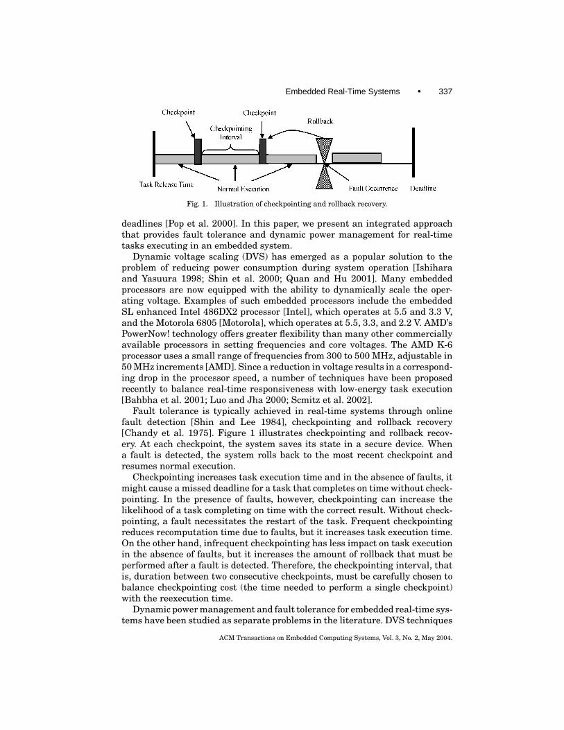
Fig. 1. Illustration of checkpointing and rollback recovery.

deadlines [Pop et al. 2000]. In this paper, we present an integrated approachthat provides fault tolerance and dynamic power management for real-timetasks executing in an embedded system.

Dynamic voltage scaling (DVS) has emerged as a popular solution to theproblem of reducing power consumption during system operation [Ishiharaand Yasuura 1998; Shin et al. 2000; Quan and Hu 2001]. Many embeddedprocessors are now equipped with the ability to dynamically scale the oper-ating voltage. Examples of such embedded processors include the embeddedSL enhanced Intel 486DX2 processor [Intel], which operates at 5.5 and 3.3 V,and the Motorola 6805 [Motorola], which operates at 5.5, 3.3, and 2.2 V. AMD’sPowerNow! technology offers greater flexibility than many other commerciallyavailable processors in setting frequencies and core voltages. The AMD K-6processor uses a small range of frequencies from 300 to 500 MHz, adjustable in50 MHz increments [AMD]. Since a reduction in voltage results in a correspond-ing drop in the processor speed, a number of techniques have been proposedrecently to balance real-time responsiveness with low-energy task execution[Bahbha et al. 2001; Luo and Jha 2000; Scmitz et al. 2002].

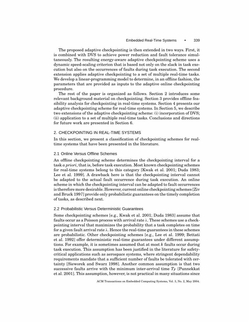
Fault tolerance is typically achieved in real-time systems through onlinefault detection [Shin and Lee 1984], checkpointing and rollback recovery[Chandy et al. 1975]. Figure 1 illustrates checkpointing and rollback recov-ery. At each checkpoint, the system saves its state in a secure device. Whena fault is detected, the system rolls back to the most recent checkpoint andresumes normal execution.

Checkpointing increases task execution time and in the absence of faults, itmight cause a missed deadline for a task that completes on time without check-pointing. In the presence of faults, however, checkpointing can increase thelikelihood of a task completing on time with the correct result. Without check-pointing, a fault necessitates the restart of the task. Frequent checkpointingreduces recomputation time due to faults, but it increases task execution time.On the other hand, infrequent checkpointing has less impact on task executionin the absence of faults, but it increases the amount of rollback that must beperformed after a fault is detected. Therefore, the checkpointing interval, thatis, duration between two consecutive checkpoints, must be carefully chosen tobalance checkpointing cost (the time needed to perform a single checkpoint)with the reexecution time.

Dynamic power management and fault tolerance for embedded real-time sys-tems have been studied as separate problems in the literature. DVS techniques

ACM Transactions on Embedded Computing Systems, Vol. 3, No. 2, May 2004.

338 • Y. Zhang and K. Chakrabarty

for power management do not consider fault tolerance [Ishihara and Yasuura1998; Shin et al. 2000; Quan and Hu 2001], and checkpoint placement strate-gies for fault tolerance do not address dynamic power management [Shin et al.1987; Ziv and Bruck 1997; Kwak et al. 2001]. However, lower processor voltagesand shrinking process technologies in the nanotechnology realm are likely tolead to lower noise margins and more transient faults, caused in part by single-event upsets [Dupont et al. 2002]. Hence a dynamic adaptation framework inwhich DVS techniques are tied to system-level fault tolerance, are of partic-ular interest for embedded systems. We present here an integrated approachthat facilitates fault tolerance through checkpointing and power managementthrough DVS. To the best of our knowledge, this is the first approach that ad-dresses these two issues in conjunction.

We assume throughout that faults are intermittent or transient in nature,and that permanent faults are handled through manufacturing testing or field-testing techniques [Bushnell and Agrawal 2000]. Typical examples of transientfaults include errors caused by cosmic rays and high-energy particles in nan-otechnology with shrinking processes [Dupont et al. 2002].

We address both hard and soft real-time systems in this paper. Systems inwhich a missed deadline results in disastrous consequences are termed hardreal-time systems, while systems in which a missed deadline results in de-graded performance, but with no extreme consequences, are termed soft real-time systems [Liu 2000]. Examples of power-constrained hard real-time sys-tems include battery-driven autonomous airborne and seaborne systems. Stockprice quotation systems, telephone switching systems, and multimedia appli-cations are examples of soft real-time systems. Therefore, it is important toguarantee timeliness for hard real-time systems in worst-case scenarios, andprovide a high likelihood of meeting task deadlines for soft real-time systems. Inthis work, the offline feasibility analysis is targeting at providing deterministictimeliness for hard real-time systems, and adaptive checkpointing is aimingat ensuring a high probability that task deadlines are met for soft real-timesystems.

We first present feasibility tests for checkpointing schemes that use a fixedcheckpointing interval for real-time tasks. These feasibility tests provide thecriteria under which checkpointing can provide fault tolerance and real-timeguarantees under two different transient fault arrival models. We also presenttwo techniques to determine the fixed checkpointing interval in an offline man-ner. Following this, we present an adaptive checkpointing scheme for real-timesystems in which a variable checkpointing interval is dynamically adjusted dur-ing task execution, and checkpoints are inserted based not only on the availableslack, but also on the occurrences of faults during task execution. This approachis in contrast to “static” checkpointing schemes that fix the checkpointing in-terval a priori before task execution. Simulation results show that comparedto previous methods, the proposed adaptive checkpointing approach increasesthe likelihood of timely task completion in the presence of faults. The proposedadaptive checkpointing is tailored to handle not only a random fault-arrivalprocess, but it is also designed to be k-fault-tolerant—it attempts to tolerate upto k fault occurrences.



The proposed adaptive checkpointing is then extended in two ways. First, itis combined with DVS to achieve power reduction and fault tolerance simul-taneously. The resulting energy-aware adaptive checkpointing scheme uses adynamic speed-scaling criterion that is based not only on the slack in task exe-cution but also on the occurrences of faults during task execution. The secondextension applies adaptive checkpointing to a set of multiple real-time tasks.We develop a linear-programming model to determine, in an offline fashion, theparameters that are provided as inputs to the adaptive online checkpointingprocedure.

The rest of the paper is organized as follows. Section 2 introduces somerelevant background material on checkpointing. Section 3 provides offline fea-sibility analysis for checkpointing in real-time systems. Section 4 presents ouradaptive checkpointing scheme for real-time systems. In Section 5, we describetwo extensions of the adaptive checkpointing scheme: (i) incorporation of DVS;(ii) application to a set of multiple real-time tasks. Conclusions and directionsfor future work are presented in Section 6.

2. CHECKPOINTING IN REAL-TIME SYSTEMS

In this section, we present a classification of checkpointing schemes for real-time systems that have been presented in the literature.

2.1 Online Versus Offline Schemes

An offline checkpointing scheme determines the checkpointing interval for atask a priori, that is, before task execution. Most known checkpointing schemesfor real-time systems belong to this category [Kwak et al. 2001; Duda 1983;Lee et al. 1999]. A drawback here is that the checkpointing interval cannotbe adapted to the actual fault occurrence during task execution. An onlinescheme in which the checkpointing interval can be adapted to fault occurrencesis therefore more desirable. However, current online checkpointing schemes [Zivand Bruck 1997] provide only probabilistic guarantees on the timely completionof tasks, as described next.

2.2 Probabilistic Versus Deterministic Guarantees

Some checkpointing schemes [e.g., Kwak et al. 2001; Duda 1983] assume thatfaults occur as a Poisson process with arrival rate λ. These schemes use a check-pointing interval that maximizes the probability that a task completes on timefor a given fault arrival rate λ. Hence the real-time guarantees in these schemesare probabilistic. Other checkpointing schemes [e.g., Lee et al. 1999; Bettatiet al. 1992] offer deterministic real-time guarantees under different assump-tions. For example, it is sometimes assumed that at most k faults occur duringtask execution. This assumption has been justified in the literature for safety-critical applications such as aerospace systems, where stringent dependabilityrequirements mandate that a sufficient number of faults be tolerated with cer-tainty [Sieworek and Swarz 1998]. Another common assumption is that twosuccessive faults arrive with the minimum inter-arrival time TF [Punnekkatet al. 2001]. This assumption, however, is not practical in many situations since



it is often hard to determine appropriate value for the parameter TF . A draw-back of most deterministic checkpointing schemes is that they cannot adapt toactual fault occurrences during task execution. In view of the above reasons,we focus here on the use of a stochastic fault arrival process and a probabilis-tic checkpointing scheme, while utilizing deterministic feasibility analysis as aguideline.

2.3 Equidistant Versus Variable Checkpointing Interval

Equidistant checkpointing, as the term implies, relies on the use of a constantcheckpointing interval during task execution. This is typically used with offlinecheckpointing schemes. It has been shown in the literature that if the check-pointing cost is C and faults arrive as a Poisson process with rate λ, the meanexecution time for the task is minimum if a constant checkpointing interval of√

2C/λ is used [Duda 1983]. We refer to this as the Poisson-arrival approach.However, the minimum execution time does not guarantee timely completionof a task under real-time deadlines. It has also been shown that if the fault-freeexecution time for a task is E, the worst-case execution time for up to k faultsis minimum if the constant checkpointing interval is set to

√EC/k [Bettati

et al. 1992]. We refer to this as the k-fault-tolerant approach. A drawback withthese equidistant schemes is that they cannot adapt to actual fault arrivals.For example, due to the random nature of fault occurrences, the checkpointinginterval can conceivably be increased halfway through task execution if only afew faults occur during the first half of task execution. Therefore, we consideronline checkpointing with variable checkpointing intervals.

2.4 Constant Versus Variable Checkpointing Cost

Most prior work has been based on the assumption that all checkpoints take thesame amount of time, that is, the checkpointing cost is constant. An alternativeadaptive approach, taken in Ziv and Bruck [1997], but less well understood, is toassume that the checkpointing cost depends on the time at which it is taken. Weuse the constant checkpointing cost model in our work because of its inherentsimplicity.

3. OFFLINE FEASIBILITY ANALYSIS

We are given a set 0 = {τ1, τ2, . . . , τn} of n periodic real-time tasks, where taskτi is modeled by a tuple τi = (Ti, Di, Ei). The elements of the tuple are definedas follows:r Ti is the period of τ i.r Di is the deadline (Di ≤ Ti for τi).r Ei is the execution time of τ i under fault-free conditions.

Let the checkpointing cost be C. We make the following assumptions relatedto task execution and fault arrivals:r The task set 0 is scheduled using fixed-priority methods such as the rate-

monotonic scheme.



r The task set 0 is schedulable under fault-free conditions.r The priority of tasks are in decreasing order of the index i, that is, task τ ihas higher priority than task τ j if i < j .r Each instance of the task is released at the beginning of the period.r The checkpointing intervals are equal for the same task.r The times for rollback and state restoration are zero.r Faults are detected as soon as they occur.r No faults occur during checkpointing and rollback recovery.

In Punnekkat et al. [2001], a feasibility analysis is provided under the as-sumption that two successive faults arrive with a minimum inter-arrival timeTF . This implies that the time between the occurrences of two faults is at leastTF . This assumption is not practical for realistic applications, where the faultoccurrence can be bursty or memoryless. For example, it is difficult to obtain aminimum inter-arrival time for a typical Poisson-arrival process. Therefore, wefocus here on tolerating up to a given number of faults during task execution.No additional assumption is made regarding fault arrivals.

Since the task set is periodic, the total execution time can be very high if weconsider a large number of periods. We therefore need to identify an appropri-ate k-fault-tolerant condition for shorter time duration. Here we provide twosolutions corresponding to two different fault-tolerance requirements. One isto tolerate k faults for each job; the other is to tolerate k faults within a hy-perperiod, which is defined the least common multiple of all the task periods[Liu 2000]. In practical situations, the choice of an appropriate fault tolerancecriterion can be made based on the needs of the applications.

We first consider the case of a single job. Suppose m(m ≥ 0) checkpointsare inserted equidistantly during the computation time to tolerate k faults inone job. The worst-case response time R for the jobis composed of three terms:the task execution time E, the checkpointing cost mC, and the recovery costkE/(m+ 1), that is, R = E +mC+ kE/(m+ 1).

To satisfy the deadline constraint, we must have E +mC+ kE/(m+ 1) ≤ D.Let f (m) = E +mC+ kE/(m+ 1)− D. The minimum value of f (m) is obtainedfor m = m0 =

√kE/C − 1. Since m is a non-negative integer, we have m0 =

dmax(√

kE/C − 1, 0)e.If f (m0) ≤ 0, there exists equidistant checkpointing schemes for k-fault-

tolerance, and the response time is minimum when m0 checkpoints are inserted.If f (m0) > 0, then no equidistant checkpointing schemes exists for toleratingup to k faults.

Example 1. For a real-time job with parameters C = 10, k = 1, E = 9,000and D = 10,000, we get m0 = 29 and f (m0) = −410. This implies that thereexists an equidistant checkpointing scheme to tolerate a single fault for this job,and the response time is minimized when 29 checkpoints are inserted. Now wechange k from 1 to 3, that is, the system is required to tolerate up to threefaults. Then we get m0 = 51 and f (m0) = 29. Since f (m0) > 0, no equidistantcheckpointing scheme exists to tolerate up to three faults for this job.



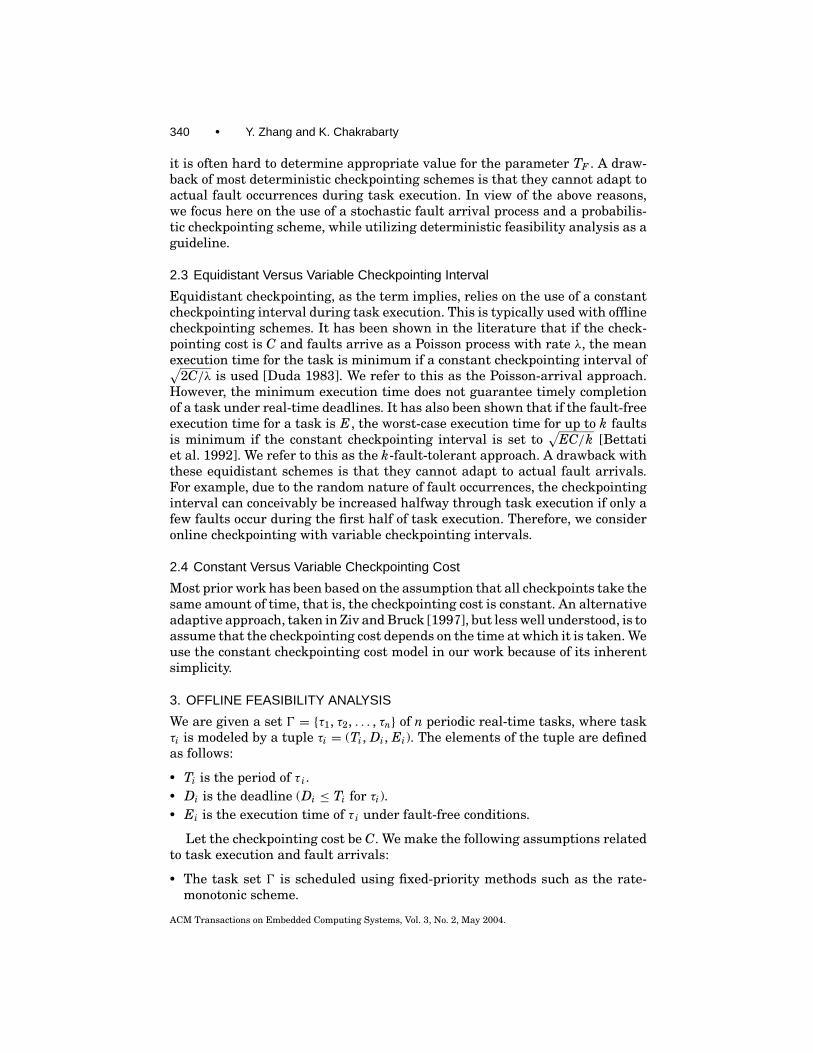
Fig. 2. Illustration of the iterative approach to determine the response time using time-demandanalysis.

3.1 Tolerating k Faults in Each Job for Multiple Tasks

In this case, we require that the task set can meet the deadline requirementunder the condition that at most k faults occur during the execution of each job.The feasibility analysis is based on the time-demand analysis for fixed-priorityscheduling [Liu 2000]. The steps in the analysis are as following:

(1) Compute the response time Ri for τ i according to the equation below (theright hand is defined as the time-demand function):

Ri = Ei +i−1∑h=1

⌈Ri

Th

⌉Eh.

Here Th and Eh are the period and the execution time of a task τh withhigher priority than τi.

This equation can be solved by forming a recurrence relation:

R( j+1)i = Ei +

i−1∑h=1

⌈R( j )

i

Th

⌉Eh. (1)

(2) The iteration is terminated either when R( j+1)i = R( j )

i and R( j )i ≤ Di for

some i or when R ( j+1)i > Di, whichever occurs sooner. In the former case, τi

is schedulable; in the later case, τi is not schedulable.

Figure 2 illustrates the iterative algorithm to determine the response timeusing time-demand analysis. The staircase function represents the magnitudeof the time-demand function. The straight line simply represents Ri. Startingfrom the original, the iterative method finds the point of intersection of thestaircase function and the straight line.

According to Liu [2000], the time complexity of the time-demand analysis foreach task is O(nW ), where W is the ratio of the largest period to the smallestperiod.



Under faulty conditions, the additional time due to checkpointing and re-covery should be incorporated. When there are m j equidistant checkpoints foreach instance of τ j , we have:

Ri =(

Ei +miC + kEi

mi + 1

)+

i−1∑h=1

⌈Ri

Th

⌉(Eh +mhC + k

Eh

mh + 1

)To minimize all response times, we must have: m∗i = dmax(

√kEi/C − 1, 0)e

(1 ≤ i ≤ n).Then we can employ the recurrence equation as follows:

R( j+1)i =

(Ei +m∗i C + k

Ei

m∗i + 1

)+

i−1∑h=1

⌈R( j )

i

Th

⌉(Eh +m∗hC + k

Eh

m∗h + 1

).

When R ( j+1)i = R( j )

i and R( j )i ≤ Di for some j , τi is schedulable; when R( j+1)

i >

Di, τi is not schedulable.

Example 2. Consider a task set composed of two tasks: τ1 = (60, 18, 7)and τ2 = (80, 34, 8), and let k = 3, C = 1. Then m∗1 = 4 and m∗2 = 4. Afterapplying the recurrence equation, we get the response times: R1 = 15.2 < 18and R2 = 33 < 34. Thus checkpointing is feasible for this task set if up to threefaults occur during each job. Next we examine the case of k = 4. For this casem∗1 = 5 and m∗2 = 5. The response times are R1 = 16.7 < 18 and R2 = 35 > 34.As a result, checkpointing is not feasible if up to four faults need to be toleratedfor each job.

3.2 Tolerating k Faults in a Hyperperiod for Multiple Tasks

In Punnekkat et al. [2001], an algorithm is presented to determine the check-pointing interval under the assumption that two successive faults arrive witha minimum inter-arrival time TF . Let F j , 1 ≤ j ≤ i, be the extra computa-tion time needed by τ j , 1 ≤ j ≤ i, if one fault occurs during the execution.When there are m j equidistant checkpoints for τ j , the response time Ri for τiis expressed as follows [Punnekkat et al. 2001]:

Ri = (Ei+miC)+i−1∑h=1

⌈Ri

Th

⌉(Eh+mhC)+

⌈Ri

TF

⌉max1≤ j≤i{F j }, where F j = E j

m j + 1.

The checkpoint is examined starting from high-priority tasks to low-prioritytasks. For each task τ j , the algorithm tries to reduce the response time byreducing the maximum additional computation time, that is, max1≤ j≤i{F j }.The details of the steps in Punnekkat et al. [2001] are as follows:

(1) Initially mi = 0 for 1 ≤ i ≤ n.(2) Starting from the highest-priority task τ1, calculate the minimum number

of checkpoints m1 required to make it schedulable.(3) In decreasing order of task priorities, calculate the response time Ri of task

τi. If Ri ≤ Di, move to the next task; otherwise Ri need to be reduced further.



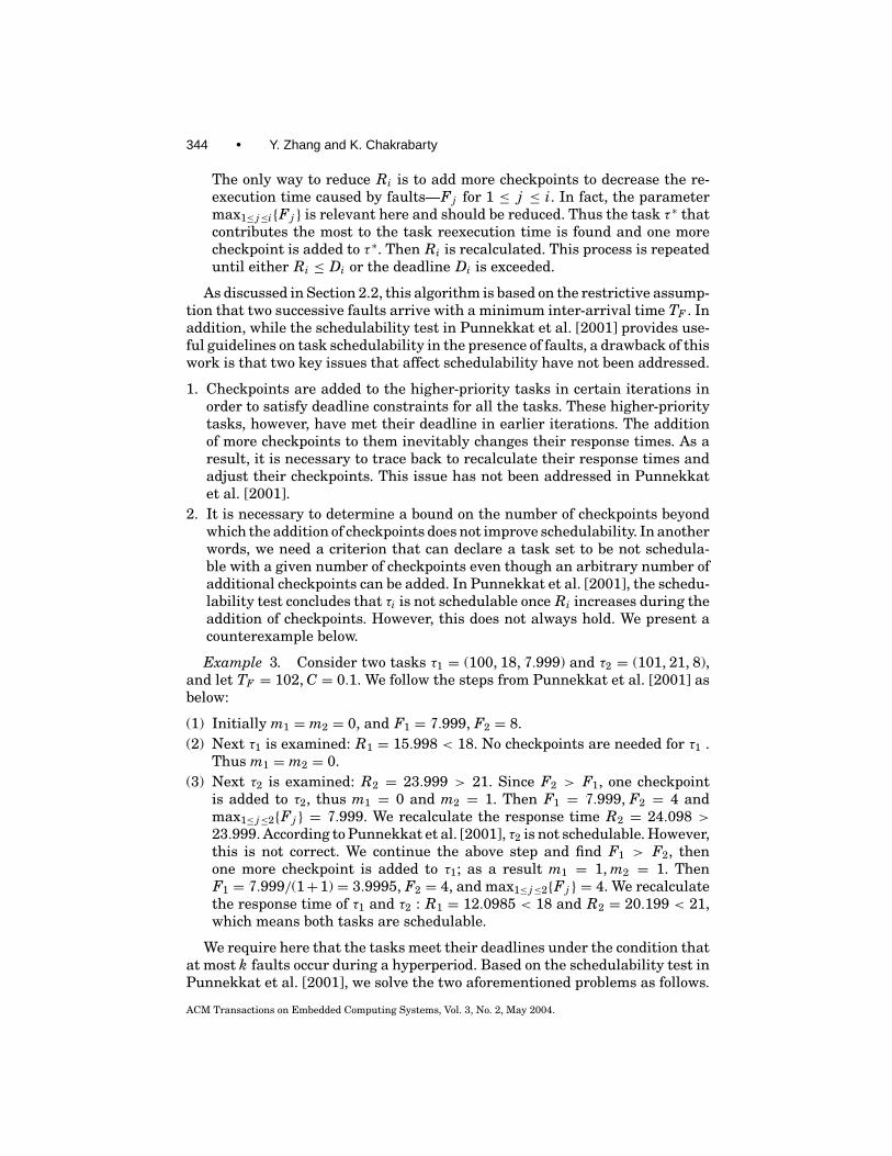
The only way to reduce Ri is to add more checkpoints to decrease the re-execution time caused by faults—F j for 1 ≤ j ≤ i. In fact, the parametermax1≤ j≤i{F j } is relevant here and should be reduced. Thus the task τ ∗ thatcontributes the most to the task reexecution time is found and one morecheckpoint is added to τ ∗. Then Ri is recalculated. This process is repeateduntil either Ri ≤ Di or the deadline Di is exceeded.

As discussed in Section 2.2, this algorithm is based on the restrictive assump-tion that two successive faults arrive with a minimum inter-arrival time TF . Inaddition, while the schedulability test in Punnekkat et al. [2001] provides use-ful guidelines on task schedulability in the presence of faults, a drawback of thiswork is that two key issues that affect schedulability have not been addressed.

1. Checkpoints are added to the higher-priority tasks in certain iterations inorder to satisfy deadline constraints for all the tasks. These higher-prioritytasks, however, have met their deadline in earlier iterations. The additionof more checkpoints to them inevitably changes their response times. As aresult, it is necessary to trace back to recalculate their response times andadjust their checkpoints. This issue has not been addressed in Punnekkatet al. [2001].

2. It is necessary to determine a bound on the number of checkpoints beyondwhich the addition of checkpoints does not improve schedulability. In anotherwords, we need a criterion that can declare a task set to be not schedula-ble with a given number of checkpoints even though an arbitrary number ofadditional checkpoints can be added. In Punnekkat et al. [2001], the schedu-lability test concludes that τi is not schedulable once Ri increases during theaddition of checkpoints. However, this does not always hold. We present acounterexample below.

Example 3. Consider two tasks τ1 = (100, 18, 7.999) and τ2 = (101, 21, 8),and let TF = 102, C = 0.1. We follow the steps from Punnekkat et al. [2001] asbelow:

(1) Initially m1 = m2 = 0, and F1 = 7.999, F2 = 8.(2) Next τ1 is examined: R1 = 15.998 < 18. No checkpoints are needed for τ1 .

Thus m1 = m2 = 0.(3) Next τ2 is examined: R2 = 23.999 > 21. Since F2 > F1, one checkpoint

is added to τ2, thus m1 = 0 and m2 = 1. Then F1 = 7.999, F2 = 4 andmax1≤ j≤2{F j } = 7.999. We recalculate the response time R2 = 24.098 >

23.999. According to Punnekkat et al. [2001], τ2 is not schedulable. However,this is not correct. We continue the above step and find F1 > F2, thenone more checkpoint is added to τ1; as a result m1 = 1, m2 = 1. ThenF1 = 7.999/(1+1) = 3.9995, F2 = 4, and max1≤ j≤2{F j } = 4. We recalculatethe response time of τ1 and τ2 : R1 = 12.0985 < 18 and R2 = 20.199 < 21,which means both tasks are schedulable.

We require here that the tasks meet their deadlines under the condition thatat most k faults occur during a hyperperiod. Based on the schedulability test inPunnekkat et al. [2001], we solve the two aforementioned problems as follows.



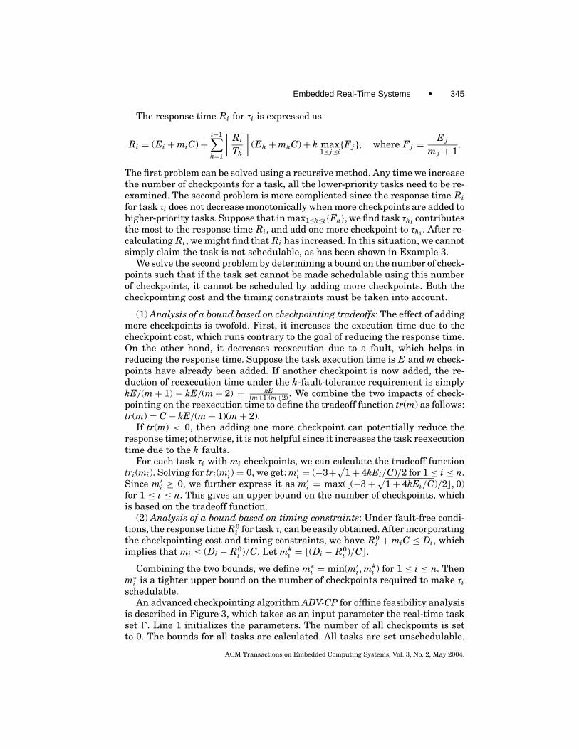
The response time Ri for τi is expressed as

Ri = (Ei +miC)+i−1∑h=1

⌈Ri

Th

⌉(Eh +mhC)+ k max

1≤ j≤i{F j }, where F j = E j

m j + 1.

The first problem can be solved using a recursive method. Any time we increasethe number of checkpoints for a task, all the lower-priority tasks need to be re-examined. The second problem is more complicated since the response time Rifor task τi does not decrease monotonically when more checkpoints are added tohigher-priority tasks. Suppose that in max1≤h≤i{Fh}, we find task τh1 contributesthe most to the response time Ri, and add one more checkpoint to τh1 . After re-calculating Ri, we might find that Ri has increased. In this situation, we cannotsimply claim the task is not schedulable, as has been shown in Example 3.

We solve the second problem by determining a bound on the number of check-points such that if the task set cannot be made schedulable using this numberof checkpoints, it cannot be scheduled by adding more checkpoints. Both thecheckpointing cost and the timing constraints must be taken into account.

(1) Analysis of a bound based on checkpointing tradeoffs: The effect of addingmore checkpoints is twofold. First, it increases the execution time due to thecheckpoint cost, which runs contrary to the goal of reducing the response time.On the other hand, it decreases reexecution due to a fault, which helps inreducing the response time. Suppose the task execution time is E and m check-points have already been added. If another checkpoint is now added, the re-duction of reexecution time under the k-fault-tolerance requirement is simplykE/(m+ 1) − kE/(m+ 2) = kE

(m+1)(m+2) . We combine the two impacts of check-pointing on the reexecution time to define the tradeoff function tr(m) as follows:tr(m) = C − kE/(m+ 1)(m+ 2).

If tr(m) < 0, then adding one more checkpoint can potentially reduce theresponse time; otherwise, it is not helpful since it increases the task reexecutiontime due to the k faults.

For each task τi with mi checkpoints, we can calculate the tradeoff functiontri(mi). Solving for tri(m′i) = 0, we get: m′i = (−3+√1+ 4kEi/C)/2 for 1 ≤ i ≤ n.Since m′i ≥ 0, we further express it as m′i = max(b(−3+√1+ 4kEi/C)/2c, 0)for 1 ≤ i ≤ n. This gives an upper bound on the number of checkpoints, whichis based on the tradeoff function.

(2) Analysis of a bound based on timing constraints: Under fault-free condi-tions, the response time R0

i for task τi can be easily obtained. After incorporatingthe checkpointing cost and timing constraints, we have R0

i +miC ≤ Di, whichimplies that mi ≤ (Di − R0

i )/C. Let m#i = b(Di − R0

i )/Cc.Combining the two bounds, we define m∗i = min(m′i, m#

i ) for 1 ≤ i ≤ n. Thenm∗i is a tighter upper bound on the number of checkpoints required to make τischedulable.

An advanced checkpointing algorithm ADV-CP for offline feasibility analysisis described in Figure 3, which takes as an input parameter the real-time taskset 0. Line 1 initializes the parameters. The number of all checkpoints is setto 0. The bounds for all tasks are calculated. All tasks are set unschedulable.



Fig. 3. Advanced checkpointing procedure.

Fig. 4. Recursive checkpointing procedure.

Line 2 calls the recursive checkpointing subroutine CP to add checkpoints fromτ1 to τn.

The recursive checkpointing procedure CP(p, q) is described in Figure 4,where p and q are the lowest and highest index for the task subset under con-sideration. Line 1 checks the deadline constraint to see if the current numberof checkpoints can make the task subset schedulable. Line 2 checks to see if thebounds for the task subset are exceeded. If so, the whole task set is unschedula-ble and the recursive checkpointing should be exited. Line 3 further improvesthe feasibility of tasks from τp to τq . Line 3.1 calculates R j . If the deadlinecannot be met for τ j using the current number of checkpoints, Line 3.2 addsmore checkpoints to higher-priority tasks or to τ j itself. Line 3.2.1 finds thetask τh that contributes most to the task reexecution time. Line 3.2.2 adds onemore checkpoint to τh, and Line 3.2.3 recalculates the reexecution time due toτh. Finally, Line 3.2.4 employs the procedure CP for tasks from τh to τ j .

The time complexity for the feasibility test and the checkpointing procedurecan be analyzed as follows. The computation of m∗i for all the tasks takes O(n2W )in the worst case. Each time a checkpoint is added, the response time for lower-priority tasks need to be recalculated. Hence the recursive execution of CP(p, q)takes O(n2W )

∑ni=1 m∗i . Let M ∗ =∑n

i=1 m∗i . Adding all the cost together, the to-tal complexity is O(n2WM∗), which is only quadratic in the number of tasks n.Furthermore, we note that the complexity can be reduced if we can make



M ∗ as small as possible. That is why we combine both the tradeoff functionand timing constraints to obtain a relatively tight bound for m∗i .

4. ADAPTIVE CHECKPOINTING

In the adaptive checkpointing scheme, the actual fault arrival process is mod-eled as a Poisson process with rate λ. At the same time, our goal is to tolerateup to k faults for each job during task execution. We first limit ourselves toa single job here, and then outline the extension to a set of multiple periodictasks.

We next determine the maximum value of E for the Poisson-arrival andthe k-fault-tolerant schemes beyond which these schemes will always miss thejob deadline. Our proposed adaptive checkpointing scheme is more likely tomeet the task deadline even when E exceeds these threshold values. If thePoisson-arrival scheme is used, the effective task execution time in the absenceof faults must be less than the deadline D if the probability of timely completionof the task in the presence of faults is to be nonzero. This implies that E +[E/(

√2C/λ)− 1]C ≤ D, from which we get the threshold:

Eλth = (D + C)/(1+√λC/2) (2)

Here [E/(√

2C/λ)− 1] refers to the number of checkpoints. The reexecutiontime due to rollback is not included in the formula for Eλth. If E exceeds Eλthfor the Poisson-arrival approach, the probability of timely completion of thetask is simply zero. Therefore, beyond this threshold, the checkpointing inter-val must be set by exploiting the slack time, instead of utilizing the optimumcheckpointing interval for the Poisson-arrival approach. The checkpointing in-terval Im that barely allows timely completion in the fault-free case is givenby E + (E/Im − 1)C = D from which it follows that Im = EC/(D + C − E). Todecrease the checkpointing cost, we set the checkpointing interval to 2Im in ouradaptive scheme.

A similar threshold on the execution time can easily be calculated for thek-fault-tolerant scheme. In order to satisfy the k-fault-tolerant requirement,the worst-case reexecution time is incorporated. The following inequality musthold:

E + [E/(√

EC/k)− 1]C + k√

EC/k ≤ D.

This implies the following threshold on E:

Ekth = [(D + C)+ 2kC]− 2√

kC(D + C)+ (kC)2 (3)

If the execution time E exceeds Ekth, the k-fault-tolerant checkpointingscheme cannot provide a deterministic guarantee to tolerate up to k faults.

4.1 Checkpointing Algorithm for a Single Job

The adaptive checkpointing algorithm attempts to maximize the probabilitythat the job completes before its deadline despite the arrival of faults as aPoisson process with rate λ. A secondary goal is to tolerate, as for a possible,



Fig. 5. (a) Procedure for calculating the checkpointing interval and (b) adaptive checkpointingprocedure.

up to k faults. In this way, the algorithm accommodates a predefined fault-tolerance requirement (handle up to k faults) as well as dynamic fault arrivalsmodeled by the Poisson process. We list below some notation that we use in ourdescription of the algorithm:

1. I1(C, λ) = √2C/λ denotes the checkpointing interval for the Poisson-arrivalapproach.

2. I2(E, k, C) = √EC/k denotes the checkpointing interval for the k-fault-

tolerant approach.3. I3(E, D, C) = 2EC/(D + C − E) denotes the checkpointing interval if the

Poisson-arrival approach is not feasible for timely task completion.4. Rt denotes the remaining execution time. It is obtained by subtracting from

E the amount of time the job has executed (not including checkpointing andrecovery). This parameter is updated during job execution.

5. Rd denotes the time left before the deadline. It is obtained by subtractingthe current time from D. This parameter is repeatedly updated during jobexecution.

6. R f denotes an upper bound on the remaining number of faults that must betolerated. This parameter is also repeatedly updated during job execution.

7. The threshold Thλ(Rd , λ, C) is obtained by replacing D with Rd in (2). Ifthe remaining time Rt is greater than this threshold, the task will miss itsdeadline even if no additional fault occurs in the system.

8. The threshold Th(Rd , R f , C) is obtained by replacing D with Rd and k withR f in (3). If the remaining time Rt is greater than this threshold, the R f -fault-tolerant requirement cannot be satisfied.

The procedure interval (Rd , Rt , C, R f ,λ) for calculating the checkpointinginterval is described in Figure 5(a), and the adaptive checkpointing schemeadapchp(D, E, C, k, λ) is described in Figure 5(b). The adaptive checkpointingprocedure is event driven and the checkpointing interval is adjusted when afault occurs and rollback recovery is performed.



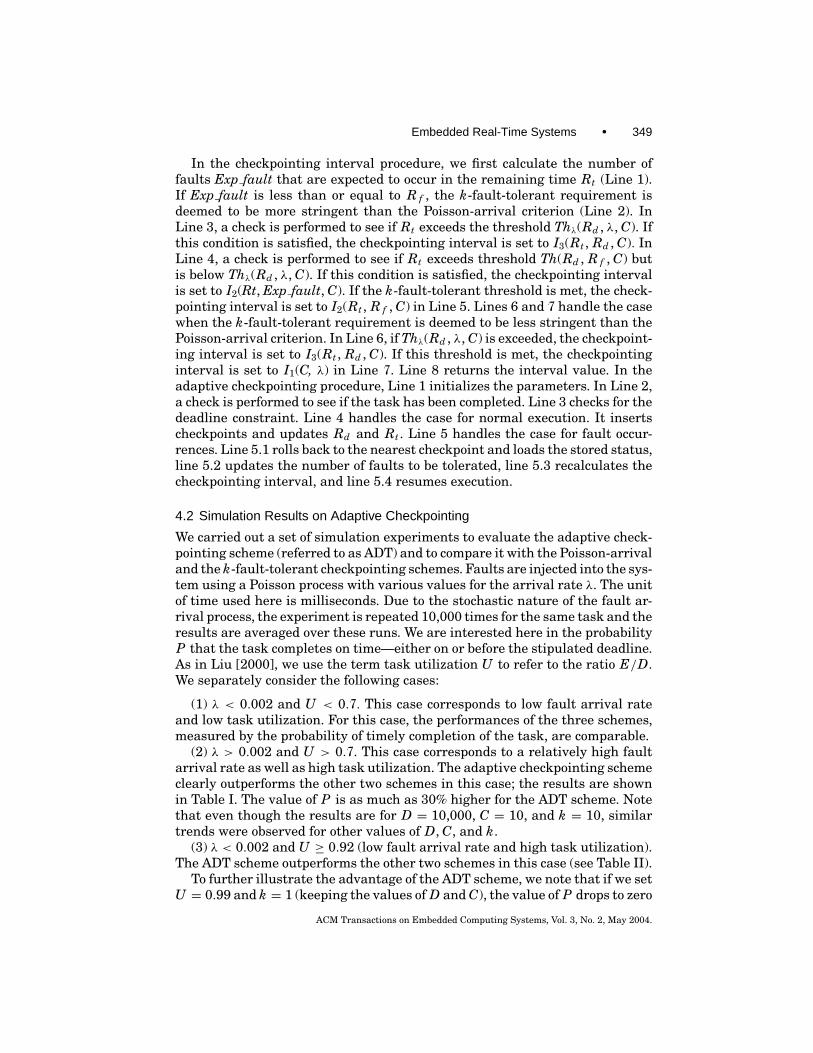
In the checkpointing interval procedure, we first calculate the number offaults Exp fault that are expected to occur in the remaining time Rt (Line 1).If Exp fault is less than or equal to R f , the k-fault-tolerant requirement isdeemed to be more stringent than the Poisson-arrival criterion (Line 2). InLine 3, a check is performed to see if Rt exceeds the threshold Thλ(Rd , λ, C). Ifthis condition is satisfied, the checkpointing interval is set to I3(Rt , Rd , C). InLine 4, a check is performed to see if Rt exceeds threshold Th(Rd , R f , C) butis below Thλ(Rd , λ, C). If this condition is satisfied, the checkpointing intervalis set to I2(Rt, Exp fault, C). If the k-fault-tolerant threshold is met, the check-pointing interval is set to I2(Rt , R f , C) in Line 5. Lines 6 and 7 handle the casewhen the k-fault-tolerant requirement is deemed to be less stringent than thePoisson-arrival criterion. In Line 6, if Thλ(Rd , λ, C) is exceeded, the checkpoint-ing interval is set to I3(Rt , Rd , C). If this threshold is met, the checkpointinginterval is set to I1(C, λ) in Line 7. Line 8 returns the interval value. In theadaptive checkpointing procedure, Line 1 initializes the parameters. In Line 2,a check is performed to see if the task has been completed. Line 3 checks for thedeadline constraint. Line 4 handles the case for normal execution. It insertscheckpoints and updates Rd and Rt . Line 5 handles the case for fault occur-rences. Line 5.1 rolls back to the nearest checkpoint and loads the stored status,line 5.2 updates the number of faults to be tolerated, line 5.3 recalculates thecheckpointing interval, and line 5.4 resumes execution.

4.2 Simulation Results on Adaptive Checkpointing

We carried out a set of simulation experiments to evaluate the adaptive check-pointing scheme (referred to as ADT) and to compare it with the Poisson-arrivaland the k-fault-tolerant checkpointing schemes. Faults are injected into the sys-tem using a Poisson process with various values for the arrival rate λ. The unitof time used here is milliseconds. Due to the stochastic nature of the fault ar-rival process, the experiment is repeated 10,000 times for the same task and theresults are averaged over these runs. We are interested here in the probabilityP that the task completes on time—either on or before the stipulated deadline.As in Liu [2000], we use the term task utilization U to refer to the ratio E/D.We separately consider the following cases:

(1) λ < 0.002 and U < 0.7. This case corresponds to low fault arrival rateand low task utilization. For this case, the performances of the three schemes,measured by the probability of timely completion of the task, are comparable.

(2) λ > 0.002 and U > 0.7. This case corresponds to a relatively high faultarrival rate as well as high task utilization. The adaptive checkpointing schemeclearly outperforms the other two schemes in this case; the results are shownin Table I. The value of P is as much as 30% higher for the ADT scheme. Notethat even though the results are for D = 10,000, C = 10, and k = 10, similartrends were observed for other values of D, C, and k.

(3) λ < 0.002 and U ≥ 0.92 (low fault arrival rate and high task utilization).The ADT scheme outperforms the other two schemes in this case (see Table II).

To further illustrate the advantage of the ADT scheme, we note that if we setU = 0.99 and k = 1 (keeping the values of D and C), the value of P drops to zero



Table I. P Versus λ (Panel A) and P Versus U (Panel B) for D = 10,000, C = 10,and k = 10

Fault Arrival Probability of Timely Completion of Tasks, PU = E/D Rate λ (×10−2) Poisson-Arrival k-Fault-Tolerant ADT(Panel A) 0.22 0.658 0.554 0.703

0.80 0.24 0.505 0.476 0.5320.28 0.229 0.243 0.2730.30 0.152 0.151 0.199

0.82 0.22 0.313 0.276 0.3540.24 0.204 0.168 0.2350.28 0.052 0.042 0.0920.30 0.027 0.035 0.039

Probability of Timely Completion of Tasks, Pλ (×10−2) U = E/D Poisson-Arrival k-Fault-Tolerant ADT(Panel B) 0.72 0.996 0.996 0.997

0.26 0.76 0.887 0.888 0.9090.78 0.655 0.666 0.7150.80 0.357 0.369 0.394

0.30 0.72 0.995 0.996 0.9980.76 0.864 0.823 0.8720.78 0.589 0.597 0.6260.80 0.269 0.275 0.331

Table II. P Versus λ (Panel A) and P Versus U (Panel B) for D = 10,000, C = 10, and k = 1

Probability of Timely Completion of Tasks, PU = E/D Fault Arrival Rate λ (×10−4) Poisson-Arrival k-Fault-Tolerant ADT(Panel A) 1.0 0.902 0.945 0.947

0.92 2.0 0.770 0.786 0.8310.95 1.0 0.659 0.649 0.774

2.0 0.372 0.387 0.513


1.0 0.94 0.747 0.818 0.8520.96 0.589 0.578 0.643

2.0 0.92 0.770 0.786 0.8310.94 0.573 0.558 0.6430.96 0.298 0.316 0.437

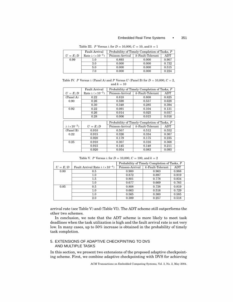
for both the Poisson-arrival and the k-fault-tolerant schemes if λ > 3 × 10−5.In contrast, the proposed ADT scheme continues to provide significant highervalue of P as λ increases (Table III).

(4) λ > 0.002 and U ≥ 0.9 (high fault arrival rate and high task utilization).Here again the ADT scheme outperforms the other two schemes (Table IV).

In many practical applications, the checkpointing cost C may be higher thanused for the above examples, and the fault arrival rate λ may be lower. Thefault arrival rate for systems operating in harsh environments has been shownto be in the range of 10−2 to 102 per hour [Punnekkat et al. 1999]. We thereforechoose value of λ in this range. To demonstrate the applicability of our schemeto such cases, we provide results for higher checkpointing cost and a lower fault



Table III. P Versus λ for D = 10,000, C = 10, and k = 1

Fault Arrival Probability of Timely Completion of Tasks, PU = E/D Rate λ (×10−5) Poisson-Arrival k-Fault-Tolerant ADT

0.99 1.0 0.893 0.000 0.9073.0 0.000 0.000 0.7325.0 0.000 0.000 0.5157.0 0.000 0.000 0.224

Table IV. P Versus λ (Panel A) and P Versus U (Panel B) for D = 10,000, C = 2,and k = 10

Fault Arrival Probability of Timely Completion of Tasks, PU = E/D Rate λ (×10−2) Poisson-Arrival k-Fault-Tolerant ADT(Panel A) 0.22 0.818 0.808 0.825

0.90 0.26 0.598 0.537 0.6280.30 0.348 0.285 0.394

0.92 0.22 0.091 0.104 0.1310.26 0.014 0.025 0.0370.28 0.006 0.015 0.016


0.22 0.915 0.326 0.334 0.3670.920 0.179 0.175 0.235

0.25 0.910 0.307 0.316 0.3680.915 0.145 0.148 0.2110.920 0.054 0.083 0.093

Table V. P Versus λ for D = 10,000, C = 100, and k = 2

Probability of Timely Completion of Tasks, PU = E/D Fault Arrival Rate λ (×10−4) Poisson-Arrival k-Fault-Tolerant ADT

0.80 0.5 0.900 0.963 0.9881.0 0.872 0.897 0.9191.5 0.801 0.778 0.8341.0 0.677 0.669 0.783

0.85 0.5 0.808 0.738 0.8191.0 0.663 0.516 0.7291.0 0.565 0.360 0.5852.0 0.389 0.257 0.518

arrival rate (see Table V) and (Table VI). The ADT scheme still outperforms theother two schemes.

In conclusion, we note that the ADT scheme is more likely to meet taskdeadlines when the task utilization is high and the fault arrival rate is not verylow. In many cases, up to 50% increase is obtained in the probability of timelytask completion.

5. EXTENSIONS OF ADAPTIVE CHECKPINTING TO DVSAND MULTIPLE TASKS

In this section, we present two extensions of the proposed adaptive checkpoint-ing scheme. First, we combine adaptive checkpointing with DVS for achieving



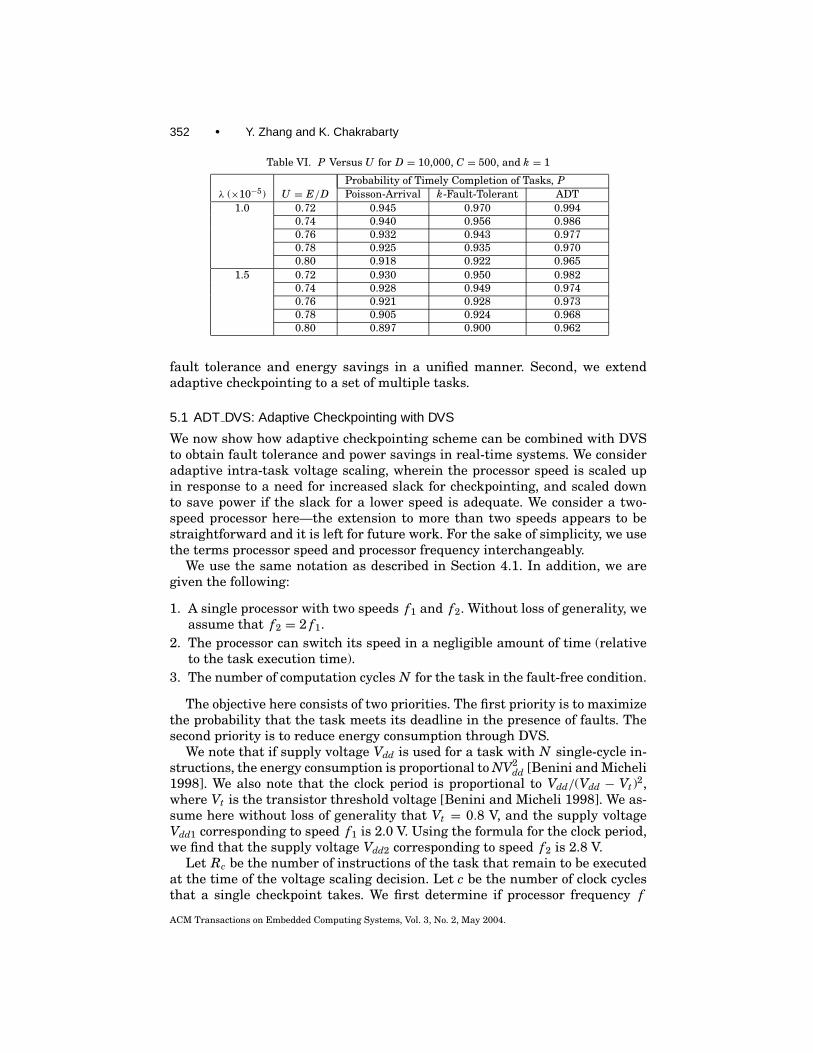
Table VI. P Versus U for D = 10,000, C = 500, and k = 1

Probability of Timely Completion of Tasks, Pλ (×10−5) U = E/D Poisson-Arrival k-Fault-Tolerant ADT

1.0 0.72 0.945 0.970 0.9940.74 0.940 0.956 0.9860.76 0.932 0.943 0.9770.78 0.925 0.935 0.9700.80 0.918 0.922 0.965

1.5 0.72 0.930 0.950 0.9820.74 0.928 0.949 0.9740.76 0.921 0.928 0.9730.78 0.905 0.924 0.9680.80 0.897 0.900 0.962

fault tolerance and energy savings in a unified manner. Second, we extendadaptive checkpointing to a set of multiple tasks.

5.1 ADT DVS: Adaptive Checkpointing with DVS

We now show how adaptive checkpointing scheme can be combined with DVSto obtain fault tolerance and power savings in real-time systems. We consideradaptive intra-task voltage scaling, wherein the processor speed is scaled upin response to a need for increased slack for checkpointing, and scaled downto save power if the slack for a lower speed is adequate. We consider a two-speed processor here—the extension to more than two speeds appears to bestraightforward and it is left for future work. For the sake of simplicity, we usethe terms processor speed and processor frequency interchangeably.

We use the same notation as described in Section 4.1. In addition, we aregiven the following:

1. A single processor with two speeds f1 and f2. Without loss of generality, weassume that f2 = 2 f1.

2. The processor can switch its speed in a negligible amount of time (relativeto the task execution time).

3. The number of computation cycles N for the task in the fault-free condition.

The objective here consists of two priorities. The first priority is to maximizethe probability that the task meets its deadline in the presence of faults. Thesecond priority is to reduce energy consumption through DVS.

We note that if supply voltage Vdd is used for a task with N single-cycle in-structions, the energy consumption is proportional to NV2

dd [Benini and Micheli1998]. We also note that the clock period is proportional to Vdd/(Vdd − Vt)2,where Vt is the transistor threshold voltage [Benini and Micheli 1998]. We as-sume here without loss of generality that Vt = 0.8 V, and the supply voltageVdd1 corresponding to speed f1 is 2.0 V. Using the formula for the clock period,we find that the supply voltage Vdd2 corresponding to speed f2 is 2.8 V.

Let Rc be the number of instructions of the task that remain to be executedat the time of the voltage scaling decision. Let c be the number of clock cyclesthat a single checkpoint takes. We first determine if processor frequency f



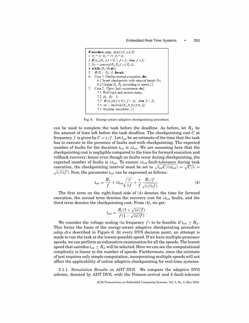
Fig. 6. Energy-aware adaptive checkpointing procedure.

can be used to complete the task before the deadline. As before, let Rd bethe amount of time left before the task deadline. The checkpointing cost C atfrequency f is given by C = c/ f . Let test be an estimate of the time that the taskhas to execute in the presence of faults and with checkpointing. The expectednumber of faults for the duration test is λtest. We are assuming here that thecheckpointing cost is negligible compared to the time for forward execution androllback recovery; hence even though no faults occur during checkpointing, theexpected number of faults is λtest. To ensure λtest-fault-tolerance during taskexecution, the checkpointing interval must be set to

√testC/(λtest) =

√C/λ =√

c/(λ f ). Now, the parameter test can be expressed as follows:

test = Rc

f+ λtest

√cλ f+ c

fRc/ f√c/(λ f )

. (4)

The first term on the right-hand side of (4) denotes the time for forwardexecution, the second term denotes the recovery cost for λtest faults, and thethird term denotes the checkpointing cost. From (4), we get:

test = Rc(1+√λc/ f )

f (1−√λc/ f ).

We consider the voltage scaling (to frequency f ) to be feasible if test ≤ Rd .This forms the basis of the energy-aware adaptive checkpointing procedureadap dvs described in Figure 6. At every DVS decision point, an attempt ismade to run the task at the lowest-possible speed. If we have multiple processorspeeds, we can perform an exhaustive examination for all the speeds. The lowestspeed that satisfies test ≤ Rd will be selected. Here we can see the computationalcomplexity is linear in the number of speeds. Furthermore, since the estimateof test requires only simple computation, incorporating multiple speeds will notaffect the applicability of online adaptive checkpointing for real-time systems.

5.1.1 Simulation Results on ADT DVS. We compare the adaptive DVSscheme, denoted by ADT DVS, with the Poisson-arrival and k-fault-tolerant



Table VII. P Versus λ (Panel A) and P Versus U (Panel B) for D = 10,000, c = 10, and k = 2

Fault Arrival Probability of Timely Completion of Tasks, PU Rate λ (×10−4) Poisson-Arrival k-Fault-Tolerant ADT DVS

(Panel A) 0.5 0.976 0.999 1.0000.90 1.0 0.963 0.991 1.000

1.5 0.942 0.988 1.0002.0 0.919 0.972 1.000

0.95 0.5 0.790 0.704 1.0001.0 0.648 0.508 1.0001.5 0.501 0.367 1.0002.0 0.385 0.244 1.000

Probability of Timely Completion of Tasks, Pλ (×10−4) U Poisson-Arrival k-Fault-Tolerant ADT DVS(Panel B) 0.92 0.924 0.960 1.000

1.0 0.94 0.750 0.735 1.0000.96 0.549 0.000 1.0000.98 0.000 0.000 1.0001.00 0.000 0.000 1.000

2.0 0.92 0.799 0.849 1.0000.94 0.530 0.439 1.0000.96 0.229 0.000 1.0000.98 0.000 0.000 1.0001.00 0.000 0.000 1.000

schemes in terms of the probability of timely completion and energy consump-tion. We use the same experimental set-up as in Section 4.2. In addition, weconsider the normalized frequency values f1 = 1 and f2 = 2. First, we as-sume that both the Poisson-arrival and the k-fault-tolerant schemes, use thelower speed f1. The task execution time at speed f1 is chosen to be less thanD—N/ f1 < D. The task utilization U in this case is simply N/( f1 D). Our ex-perimental results are shown in Table VII. The ADT DVS scheme always leadsto timely completion of the task by appropriately choosing segments of timewhen the higher frequency f2 is used. The other two schemes provide a ratherlow value for P , and for larger values of λ and U, P drops to zero. The energyconsumption for the ADT DVS scheme is slightly higher than that for the othertwo schemes; however, on average, the task runs at the lower speed f1 for asmuch as 90% of the time. The combination of adaptive checkpointing and DVSutilizes the slack effectively and stretches the task completion time to as closeto the deadline as possible.

Next we assume that both the Poisson-arrival and the k-fault-tolerantschemes use the higher speed f2. The task execution time at speed f2 is cho-sen to be less than D—N/ f2 < D, and the task utilization here is N/( f2 D).Table VIII shows that since even though ADT DVS uses both f1 and f2, adap-tive checkpointing allows it to provide a higher value for P than the othertwo methods that use only the higher speed f2. The energy consumption forADT DVS is up to 50% less than for the other two methods for low to moder-ate values of λ and U (see Table IX). When either λ or U is high, the energyconsumption of ADT DVS is comparable to that of the other two schemes. (En-ergy is measured by summing the product of the square of the voltage and the



Table VIII. P Versus λ for D = 10,000, c = 10, and k = 1

Fault Arrival Probability of Timely Completion of Tasks, PU Rate λ (×10−4) Poisson-Arrival k-Fault-Tolerant ADT DVS

0.95 0.8 0.898 0.939 0.9651.2 0.841 0.868 0.9121.6 0.754 0.785 0.8712.0 0.706 0.695 0.791

Table IX. Energy Consumption Versus λ (Panel A) and Energy ConsumptionVersus U (Panel B) for D = 10,000, c = 10, and k = 10

Fault Arrival Energy ConsumptionU Rate λ (×10−4) Poisson-Arrival k-Fault-Tolerant ADT DVS

(Panel A) 2.0 25,067 26,327 21,5680.60 4.0 25,574 26,477 21,642

6.0 25,915 26,635 21,7148.0 26,277 26,806 22,611

Energy Consumptionλ (×10−4) U Poisson-Arrival k-Fault-Tolerant ADT DVS(Panel B) 0.10 4,295 4,909 2,508

5.0 0.20 8,567 9,335 4,7910.30 12,862 13,862 7,0260.40 17,138 17,990 9,2230.50 21,474 22,300 15,333

number of computation cycles over all the segments of the task.) This is ex-pected, since ADT DVS attempts to meet the task deadline as the first priorityand if either λ or U is high, ADT DVS seldom scales down the processor speed.

5.2 Adaptive Checkpointing for Multiple Tasks

We next present the extended adaptive checkpointing procedure for a set ofmultiple tasks.

5.2.1 System Model. Our objective here is to extend the adapchp(D, E,C, k, λ) procedure to a set of multiple real-time tasks. We are given a set 0 ={τ1, τ2, . . . , τn} of n periodic tasks, where task τi is modeled by a tuple τi =(Ti, Di, Ei), Ti is the period of τi, Di is the relative deadline (Di ≤ Ti), and Ei isthe computation time under fault-free conditions. We are also aiming to tolerateup to k faults for each task instance.

The task set is first scheduled offline with a general scheduling algorithmscheme under fault-free conditions. Here we employ the earliest-deadline-first(EDF) algorithm [Liu 2000]. Alternative base scheduling techniques such as therate-monotonic algorithm can also be used. We are using EDF here to simplifythe presentation of the procedure. A sequence of m jobs 8 = {θ1, θ2, . . . , θm} isobtained for each hyperperiod. We further denote each job θi, 1 ≤ i ≤ m, asa tuple θi = 〈ai, bi, ci〉, where ai is the starting time, bi is the execution time,and ci is the deadline for θi. All these parameters are known a priori. Notethat ai is the absolute time, when θi starts execution instead of the relativerelease time, execution time is equal to that for the corresponding task, and



job deadline is equal to the task deadline plus the product of task period andcorresponding number of periods. In addition, since we are employing EDF, wehave c1 ≤ c2 ≤ · · · ≤ cm.

Based on the job set8, we develop a checkpointing scheme that inserts check-points to each job by exploiting the slacks in a hyperperiod. The key issue hereis to determine an appropriate value for the deadline that can be provided as aninput parameter to the adapchp(D, E, C, k, λ) procedure. This deadline mustbe no greater than the exact job deadline such that the timing constraint canbe met, and it should also be no less than the job execution time such that timeredundancy can be exploited for fault-tolerance. To obtain this parameter, weincorporate a preprocessing step immediately after the offline EDF schedulingis carried out. The resulting values are then provided for subsequent onlineadaptive checkpointing procedure.

We denote the slack time for job θi, 1 ≤ i ≤ m, as hi. We also introduce theconcept of checkpointing deadline vi, which is the deadline parameter providedto the adapchp(D, E, C, k, λ) procedure. It is defined as the sum of job executiontime bi and slack time hi. Furthermore, for the sake of convenience of problemformulation, we add a pseudojob θ0, which has parameters a0= b0= c0=h0= 0.The benefit of introducing θ0 will be demonstrated shortly.

5.2.2 Linear-Programming Model. Now we illustrate the preprocessingstep needed to obtain the slack time hi for each job θi, 1 ≤ i ≤ m. According tothe deadline constraints, we have

max {ai + bi + hi, ai+1} + bi+1 + hi+1 ≤ ci+1, where 0 ≤ i ≤ m− 1.

On the other hand, to ensure each job has the minimum time-redundancy forfault-tolerance, we require the slack of each job to be greater than a constantthreshold value Q , which is defined as a given number of checkpoints. Then wehave

hi ≥ Q , where 1 ≤ i ≤ m.

The problem now is that of allocating the slacks appropriately to the jobssubject to the above constraints. If we choose the total slack as the optimizationfunction, then the problem is how to maximize the sum of all slacks

∑mi=1 hi.

This is a linear-programming problem and hi can be obtained by employinglinear programming solver tools such as BPMPD [NEOS]. Since this processingstep is done offline prior to the actual execution of the job set, the additionalcomputation is acceptable. In our experiments, the CPU time is less than 1 sfor moderate problem size (number of jobs < 20). For greater problem size, theCPU time is normally less than 1 min.

5.2.3 Modification to the adapchp Procedure. After obtaining the slacks forall jobs offline through the preprocessing step, we next incorporate them into theonline adaptive checkpointing scheme. The adapchp procedure of Figure 5(b)needs to be modified due to the following reasons.

(1) In the adapchp procedure, a job is declared to be unschedulable if thedeadline is missed. When this happens, the execution of the entire set of jobs is



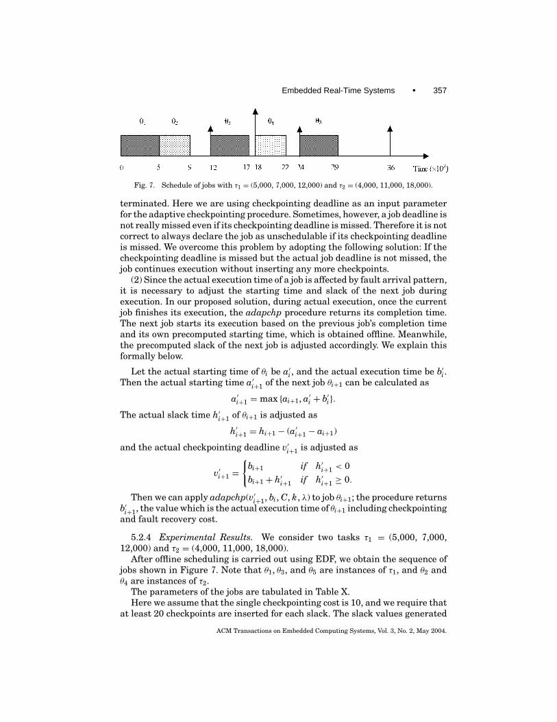
Fig. 7. Schedule of jobs with τ1 = (5,000, 7,000, 12,000) and τ2 = (4,000, 11,000, 18,000).

terminated. Here we are using checkpointing deadline as an input parameterfor the adaptive checkpointing procedure. Sometimes, however, a job deadline isnot really missed even if its checkpointing deadline is missed. Therefore it is notcorrect to always declare the job as unschedulable if its checkpointing deadlineis missed. We overcome this problem by adopting the following solution: If thecheckpointing deadline is missed but the actual job deadline is not missed, thejob continues execution without inserting any more checkpoints.

(2) Since the actual execution time of a job is affected by fault arrival pattern,it is necessary to adjust the starting time and slack of the next job duringexecution. In our proposed solution, during actual execution, once the currentjob finishes its execution, the adapchp procedure returns its completion time.The next job starts its execution based on the previous job’s completion timeand its own precomputed starting time, which is obtained offline. Meanwhile,the precomputed slack of the next job is adjusted accordingly. We explain thisformally below.

Let the actual starting time of θi be a′i, and the actual execution time be b′i.Then the actual starting time a′i+1 of the next job θi+1 can be calculated as

a′i+1 = max {ai+1, a′i + b′i}.The actual slack time h′i+1 of θi+1 is adjusted as

h′i+1 = hi+1 − (a′i+1 − ai+1)

and the actual checkpointing deadline v′i+1 is adjusted as

v′i+1 ={

bi+1 if h′i+1 < 0bi+1 + h′i+1 if h′i+1 ≥ 0.

Then we can apply adapchp(v′i+1, bi, C, k, λ) to job θi+1; the procedure returnsb′i+1, the value which is the actual execution time of θi+1 including checkpointingand fault recovery cost.

5.2.4 Experimental Results. We consider two tasks τ1 = (5,000, 7,000,12,000) and τ2 = (4,000, 11,000, 18,000).

After offline scheduling is carried out using EDF, we obtain the sequence ofjobs shown in Figure 7. Note that θ1, θ3, and θ5 are instances of τ1, and θ2 andθ4 are instances of τ2.

The parameters of the jobs are tabulated in Table X.Here we assume that the single checkpointing cost is 10, and we require that

at least 20 checkpoints are inserted for each slack. The slack values generated



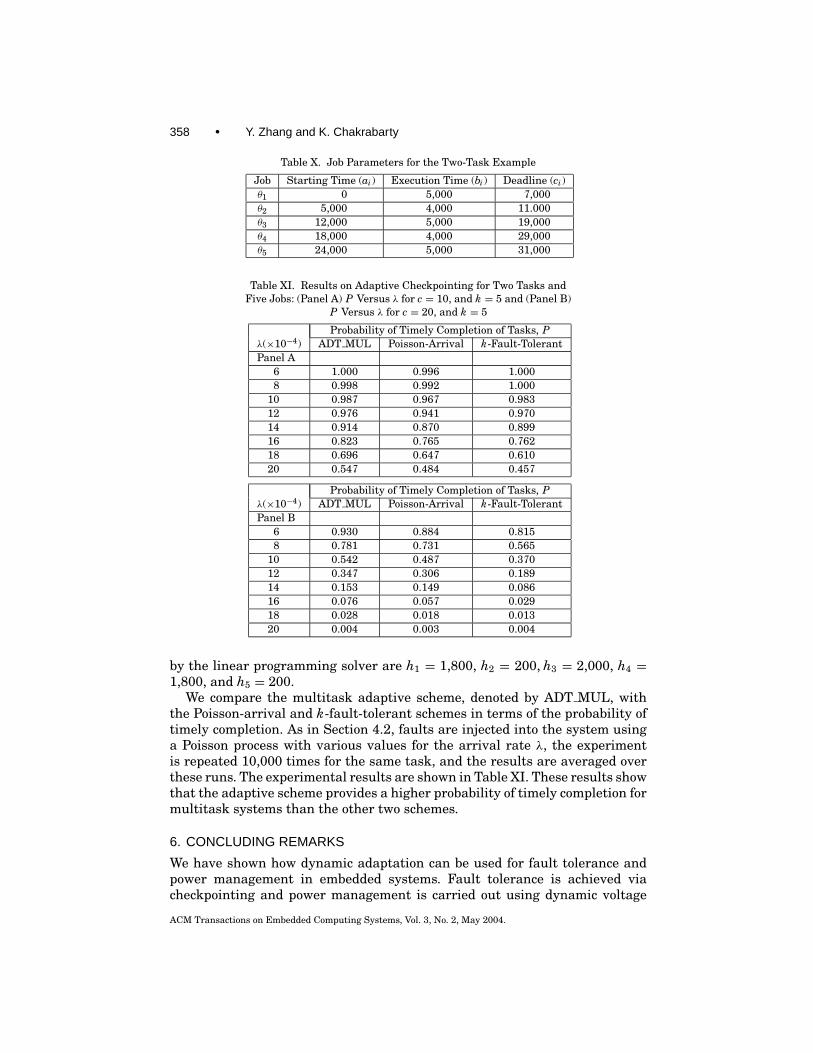
Table X. Job Parameters for the Two-Task Example

Job Starting Time (ai) Execution Time (bi) Deadline (ci)θ1 0 5,000 7,000θ2 5,000 4,000 11.000θ3 12,000 5,000 19,000θ4 18,000 4,000 29,000θ5 24,000 5,000 31,000

Table XI. Results on Adaptive Checkpointing for Two Tasks andFive Jobs: (Panel A) P Versus λ for c = 10, and k = 5 and (Panel B)

P Versus λ for c = 20, and k = 5

Probability of Timely Completion of Tasks, Pλ(×10−4) ADT MUL Poisson-Arrival k-Fault-TolerantPanel A

6 1.000 0.996 1.0008 0.998 0.992 1.000

10 0.987 0.967 0.98312 0.976 0.941 0.97014 0.914 0.870 0.89916 0.823 0.765 0.76218 0.696 0.647 0.61020 0.547 0.484 0.457

Probability of Timely Completion of Tasks, Pλ(×10−4) ADT MUL Poisson-Arrival k-Fault-TolerantPanel B

6 0.930 0.884 0.8158 0.781 0.731 0.565

10 0.542 0.487 0.37012 0.347 0.306 0.18914 0.153 0.149 0.08616 0.076 0.057 0.02918 0.028 0.018 0.01320 0.004 0.003 0.004

by the linear programming solver are h1 = 1,800, h2 = 200, h3 = 2,000, h4 =1,800, and h5 = 200.

We compare the multitask adaptive scheme, denoted by ADT MUL, withthe Poisson-arrival and k-fault-tolerant schemes in terms of the probability oftimely completion. As in Section 4.2, faults are injected into the system usinga Poisson process with various values for the arrival rate λ, the experimentis repeated 10,000 times for the same task, and the results are averaged overthese runs. The experimental results are shown in Table XI. These results showthat the adaptive scheme provides a higher probability of timely completion formultitask systems than the other two schemes.

6. CONCLUDING REMARKS

We have shown how dynamic adaptation can be used for fault tolerance andpower management in embedded systems. Fault tolerance is achieved viacheckpointing and power management is carried out using dynamic voltage



scheduling. We have presented feasibility-of-scheduling tests for checkpointingschemes that use a fixed checkpointing interval for real-time tasks. These testsprovide the criteria under which checkpointing can provide fault tolerance andreal-time guarantees. We have considered two different fault arrival models:up to k faults for a job, and up to k faults for a hyperperiod. We have alsopresented techniques to determine a fixed checkpointing interval in an offlinemanner. Following this, we have presented an adaptive checkpointing schemefor real-time systems in which a variable checkpointing interval can be deter-mined dynamically. The checkpointing interval is dynamically adjusted duringtask execution, and checkpoints are inserted based not only on the slack in taskexecution but also on the occurrences of faults during task execution. We havepresented simulation results to show that compared to previous methods, theproposed adaptive checkpointing approach increases the likelihood of timelytask completion in the presence of faults. Together with the feasibility tests,the adaptive checkpointing method provides a useful framework for depend-able computing in the presence of faults in real-time systems.

Next, we presented a unified approach for adaptive checkpointing and DVSfor a real-time task executing in an embedded system. This approach providesfault tolerance and facilitates dynamic power management. We have presentedsimulation results to show that the proposed approach significantly reducespower consumption and increases the probability of tasks completing correctlyon time despite the occurrences of faults. We have also extended the adaptivecheckpointing scheme to a set of multiple tasks. A linear-programming modelis employed in an offline manner to obtain the relevant parameters that areused by the adaptive checkpointing procedure. Simulation results show thatthe adaptive scheme is also capable of providing a high probability of timelycompletion in the presence of faults for a set of multiple tasks.

We are currently extending this work to unified checkpointing and DVS fora set of multiple tasks. We are also investigating checkpointing for distributedsystems with multiple processing elements, where data dependencies and in-ternode communication have a significant impact on the checkpointing strategy.We are examining ways to relax the restrictions of zero fault detection latency,state restoration costs, as well as the assumption of no fault occurrence dur-ing checkpointing and rollback recovery. It is quite straightforward to modelnonzero fault detection and state restoration costs. Let the single checkpointcost be C, single fault detection cost be B, and single rollback and state restora-tion cost be H, then we can incorporate the additional costs by replacing C withC′ = C+B+H in all the expressions. It appears though that it is more difficultto relax the assumption that no faults occur during checkpointing.

REFERENCES

AMD. AMD PowerNow! Technology. http://www.amd.com/epd/processors/6.32bitproc/8.amdk6fami/x24267/24267a.pdf.

BAHBHA, N., TELCH, J., AND ZITZLER, E. 2001. Hybrid global/local search strategies for DVS in em-bedded microprocessors. In Proceedings of the International Symposium on Hardware/SoftwareCodesign, 243–248.

BENINI, L. AND MICHELI, G. D. 1998. Dynamic Power Management: Design Techniques and CADTools. Kluwer Academic Publishers, Norwell, MA.



BETTATI, R., BOWEN, N. S., AND CHUNG, J. Y. 1992. Checkpointing imprecise computation. In Pro-ceedings of the IEEE Workshop on Imprecise and Approximate Computation. 45–49.

BUSHNELL, M. L. AND AGRAWAL, V. D. 2000. Essentials of Electronic Testing. Kluwer AcademicPublishers, Norwell, MA.

CHANDY, K. M., BROWNE, J. C., DISSLY, C. W., AND UHRIG, W. R. 1975. Analytic models for rollbackand recovery strategies in data base systems. IEEE Trans. Software Eng. 1 (March), 100–110.

DUDA, A. 1983. The effects of checkpointing on program execution time. Inf. Process. Lett. 16(June), 221–229.

DUPONT, E., NICOLAIDIS, M., AND ROHR, P. 2002. Embedded robustness IPs for transient-error-freeIcs. IEEE Des. Test Comput. 19, 54–68.

INTEL. Intel embedded SL Enhanced 486DX2 processor. http://www.intel.com.ISHIHARA, T. AND YASUURA, H. 1998. Voltage scheduling problem for dynamically variable voltage

processors. In Proceedings of the International Symposium on Low Power Electronics and Design.197–202.

KWAK, S. W., CHOI, B. J., AND KIM, B. K. 2001. An optimal checkpointing-strategy for real-timecontrol systems under transient faults. IEEE Trans. Reliab. 50 (Sep.), 293–301.

LEE, H., SHIN, H., AND MIN, S. 1999. Worst case timing requirement of real-time tasks with timeredundancy. In Proceedings of the Real-Time Computing Systems and Applications. 410–414.

LIU, J. W. 2000. Real-Time Systems. Prentice Hall, Upper Saddle River, NJ.LUO, J. AND JHA, N. 2000. Power-conscious joint scheduling of periodic task graphs and aperiodic

tasks in distributed real-time embedded systems. In Proceedings of the International Conferenceon Computer-Aided Design. 357–364.

MOTOROLA. Motorola 6805 processor. http://www.motorola.com.NEOS SOLVERS. http://www-neos.mcs.anl.gov/neos/server-solver-types.html.POP, P., ELES, P., AND PENG, Z. 2000. Schedulability analysis for systems with data and control

dependencies. In Proceedings of the Euromicro RTS. 201–208.PUNNEKKAT, S., BURNS, A., AND DAVIS, R. 1999. Probabilistic scheduling guarantees for fault-

tolerant real-time systems. In Proceedings of the International Conference on Dependable Com-puting for Critical Applications. 361–378.

PUNNEKKAT, S., BURNS, A., AND DAVIS, R. 2001. Analysis of checkpointing for real-time systems.Real-Time Syst. J. (Jan.), 83–102.

QUAN, G. AND HU, X. 2001. Energy efficient fixed-priority scheduling for real-time systems onvariable voltage processors. In Proceedings of the Design Automation Conference. 828–833.

SCMITZ, M. T., AL-HASHIMI, B. M., AND ELES, P. 2002. Energy efficient mapping and scheduling forDVS enabled distributed embedded systems. In Proceedings of the Design, Automation and Testin Europe Conference. 514–521.

SHIN, K. G. AND LEE, Y.-H. 1984. Error detection process—Model, design and its impact on com-puter performance. IEEE Trans. Comput. 33 (June), 529–540.

SHIN, K. G., LIN, T., AND LEE, Y. 1987. Optimal checkpointing of real-time tasks. IEEE Trans.Comput. 36 (Nov.), 1328–1341.

SHIN, Y., CHOI, K., AND SAKURAI, T. 2000. Power optimization of real-time embedded systems onvariable speed processors. In Proceedings of the International Conference on Computer-AidedDesign. 365–368.

SIEWIOREK, D. AND SWARZ, R. 1998. Reliable Computer Systems: Design and Evaluation. A. K.Peters Ltd, Natick, MA.

ZIV, A. AND BRUCK, J. 1997. An on-line algorithm for checkpoint placement. IEEE Trans. Comput.46 (Sep.), 976–985.

Received January 2003; revised July 2003; accepted August 2003


Documents

Dynamic Adaptation for Fault Tolerance and Power ...people.ee.duke.edu/~krish/p336-y_zhang.pdfDynamic Adaptation for Fault Tolerance and Power Management in Embedded Real-Time Systems