Dutch Disease as an impediment to Economic Growth of Pakistan

This paper focuses on assessing the impact of Dutch Disease on economic growth of Pakistan. In the first step, Dutch Disease is detected and then examines its link with economic growth. Annual time series data from 1981 to 2016 is used for analysis from World Development Indicators (2016). Generalized Method of moment (GMM) is used for estimation as it addresses the endogeneity and hetroscadasticity problems in the data. The estimation of Dutch Disease at an aggregate and sector level provide evidence for hindrances to economic growth in Pakistan which is the main objective of the study. The results showed that Dutch disease is harmful for industrial sector which impede output and employment generation process and hence economic growth.

Dutch Disease as an impediment to Economic Growth of Pakistan

ABSTRACT

INTRODUCTION

Shahid Hussain Javaid1

Iqbal Panhwar2

1- Shaheed Zulfikar Ali Bhutto Institute of Science & Technology, SZABIST, Karachi. Email: [email protected] 2- Bahria University, Karachi.

Dutch disease is a phenomena when increase in natural resource abundance or foreign inflows which leads to appreciation in real effective exchange rate (REER) first. In the second step, this appreciation contracts the size of tradable and non-tradable sector expands. Cordon and Neary (1982) explained the idea as “adverse effect of non-booming (natural resources) sector to booming (agriculture & industrial) sector. The booming and non-booming sectors further explained in broader perspective. Booming sector includes existed available resources e.g. mining and non-booming involved agriculture and industrial sectors. These booming and non-booming sectors are called as traded sector. The non-traded sector is services sector, which consists of transport, financial services etc. Real exchange rate appreciation reduces the value of imported goods and domestic goods become expensive. This boosts the import expenditure and exports may be reduced and lead to contraction in the tradable sector. This contraction leads to decrease in output and employment level in the economy. Hence, Dutch Disease becomes harmful for economic growth of the country.

The mechanism of Dutch disease can be elaborated as: A) starting from increase in foreign financial inflows, it raises the income of different households. This improves the demand for goods and services and for labor. It would reduce the supply of labor in the market for other sectors. If the expenditure of household increases means services sector expand and this leads to increase the cost of producing industrial and agricultural goods and contract the tradable sector. Many economists through spending and the resource movement effect explain this channel. This may have positive/negative linkages by improving the productivity in production sector. B) Consumption effect is the other channel in explaining Dutch Disease effects.

Consumption effects can be explained as; Increase in prices of goods & services within the country boost the demand for imports. This raises the demand for more foreign currency,

Keywords: Foreign inflow. Economic growth, Real exchange rate, total factor productivity

JEL Classification: F36, F40, F43

71January-June 2019JISR-MSSE Number 1Volume 17

10.31384/jisrmsse/2019.17.1.5

hence appreciates the real effective exchange rate of the concerned country. This rout also reduces the tradable portion of the economy. The mainstream economists explained different economic channels. This essay is to highlight the missing link between real exchange rate and economic growth of Pakistan.

The previous studies identified evidence of Dutch Disease in individual country as well as panel of different countries. The economists like White and Wignaraja (1992), Authokorala and Rajapatirana (2003), Rajan and Subramanian (2005) Lartey (2008), using panel and cross section data for different countries found mixed results. A single country analysis includes Oomes and Kalcheva (2007) and Algieri (2011) for Russia, Lartey (2007) for Sub Sahara Africa’ found negative Dutch Disease effects. Ogun (1995) for Nigeria, Nyoni (1995) for Tanzania, Sackey (2001) for Ghana found no Dutch Disease effects.

The main contribution of this study is not only to estimate Dutch Disease at aggregate level but also identifies which economic sector (agriculture, industry and services sector) is more affected through this disease. The highlighting feature of this study is to include the inclusive growth ideology. This led to observe impact of different sectors value added contribution on exchange rate and productivity.

This study is focused on increase in foreign inflows to show Dutch Disease evidence in Pakistan. Foreign inflows are important source of foreign exchange and important channel to enhance the productivity for developing countries. In Pakistan, remittances play pivotal role in the foreign exchange collection. Foreign inflows consist of foreign direct investment, official development assistance and worker remittances. The volume of remittance exceeds that of foreign direct investment and official development assistance. Remittances to Pakistan have seen a sharp and sustained rise in the recent years, increasing from under $1 billion in 1999 to over $19 billion today (State Bank of Pakistan, 2016). This has not gone without leaving its macroeconomic impact. This is then important to observe whether increased foreign inflows have any impact on the economic growth through increase in the productivity of the country concerned. When foreign inflows come in the economy, it increases the productive capacity and changes the consumption pattern of the economy concerned. It has its impact on production, consumption and infrastructure as well.

This study examines the annual time series data about foreign inflows and empirical evidence on the existence of the disease. Identifying the sector of production, which is impediment for economic growth, is another main finding of the paper. Taking proxy for economic growth as total factor productivity (TFP) as dependent variables whereas trade openness, terms of trade, aggregate foreign inflows, government expenditure, real effective exchange rate and broad money as the independent variables, this study seeks existence of Dutch Disease. The study empirically estimates Dutch disease effects in Pakistan between 1981 and 2015 and explore whether Dutch disease is impediment to economic growth or assisting the prosperity process in case of Pakistan.

This study helps businesses and policy makers in boosting exports of goods & services. It also helps the economists in knowing the mechanism behind the increase in prices of imported and exported goods. This study is relevant to the academic researcher in understanding the relationship between foreign inflows, real effective exchange rate and productivity growth. The study helps political government in designing policies with regard to accepting different foreign inflows needed and sectoral allocation for the economic growth.72 January-June 2019 JISR-MSSENumber 1Volume 17

The research work consists of five sections. The first section deals with the introduction of the study, section two reviews literature. Section three; deal with the research methodology whereas section four presents analysis and estimation. The last section concludes the overall results and suggestions based on the analysis.


LITERATURE REVIEWBefore discussing the gap in literature and justification of this study, following is the literature reviewed. Country wise evidence of Dutch Disease is observed in the literature.

Aghion et al (2009) investigated empirical evidence that real exchange rate volatility can have a significant impact on productivity growth. The study worked on 83 countries using annual data from 1960-2000. The study found that effects of real exchange rate on economic growth are insignificant. This study uses annual data of real exchange rate, government expenditure, terms of trade, trade openness, interactive variable like overvaluation with financial development and dummy variable of currency crisis. The study lacks further analysis on different characteristics of countries, which are different in nature, and terms of governance.

Attah-Obeng (2012) investigated exchange rate and economic growth relation in Ghana using data from1980 to 2012. The focus of this study is purely applying econometric tests on the variable. The presence of autocorrelation, hetroscadasticity and multicollinearity is tested. This study confirms the theory that depreciation encourages economic growth and appreciation is bad for the Ghanaian economy. The study establishes the econometric relationship and not investigated other linking factors and channels, which connect with economic growth. Productivity again would be the possible linking variable in this regard.

Azid et al (2005) investigated the link between exchange rate volatility and economic growth. The objective of the study was to determine the negative, positive or no relationship between these variables. Theory suggests a direct link between exchange rate volatility and economic performance in the presence of open economies. The study found a negative link between exchange rate volatility and economic growth in Pakistan. The study is important which provide evidence of volatile exchange rate have negative impact on the economic growth process. The study lacks to link this with productivity variable.

Brahmbhatt and Canuto (2010) worked on the impact of Dutch Disease on a project in the World Bank. This work on Dutch disease, reflect changes in the structure of production in thewake of a favorable shock (e.g., capital inflows). The annual time series data from 1973-2010 is used. The variables of interest are FDI, REM, ODA, GDPPCI, GEXP etc. This paper identified that manufacturing sector is based on the improvement in the productivities of different sectors. Dutch Disease is bad if productivity is not increased .As for as the policy is concerned they argued only those foreign financial inflows should be welcomed having no impact on the appreciation or depreciation in the real effective exchange rate. The study used model includes total factor productivity as dependent variable and export to import ratio, government expenditure and foreign inflows as the independent variable. Bayesian technique is used to estimate the effects or existence if Dutch Disease in the developing countries.

Botta et al (2015) investigated the economic growth process in Colombia. The study found the evidence of Dutch disease in the economy concerned. The study primarily worked on the

74 January-June 2019 JISR-MSSENumber 1Volume 17

financial viability of the Dutch disease effects. The study found that real exchange rate appreciation and heavy increase in the foreign inflows put pressure on the economy and manages these pressures using productivity channel. The study only investigated the evidence of Dutch disease but not solidly tackle the issue why it occurred and how to resolve the issue if the problem continuously recurring.

Botta (2014) investigated medium term and long term macroeconomic impact of Dutch disease. The study focus on the effects of Dutch disease on financial markets. This study analyses foreign inflows and real exchange appreciation as impediment to economic growth in developing countries. The author laid stress on process of production and exports to control through real exchange rate stability. The results of the study suggest focusing on the stable exchange rate and controlled foreign inflows to achieve macroeconomic stability in the economy. The study recommends removing minimum wage regulation and supporting infrastructural investment raising overall factor productivity.

Cakrani (2013) investigated relationship between real exchange rate misalignment and government spending. The study assesses Albanian govt expenditure causing exchange rate to appreciate or depreciate. The study applied log linear model using quarterly data. The study found that govt expenditure appreciated the real exchange rate in Albanian economy since it has negative implication on employment. This study models the dependent variable (real exchange rate), with government spending, foreign direct investment, openness, remittances and real GDP per capita as independent variables. The results of the study were identifying factors responsible for a slowdown in the growth of TFP during the 90s are the effect of recent vintages of capital characterized by underutilization, fall in real public development expenditure and stagnation of manufactured exports. The paper suggested a package of policies designed to boost the growth in TFP and thereby enhance once again the growth rate of the economy.

Farid and Mazhar (2013) looked for symptoms of Dutch disease in the Pakistani economy taking into account. The methodology used by them captured endogeneity due to the managed float of Pakistani Rupee over the econometric issues in model suggested. The viewpoint is to address whether Remittances cause an appreciation of the real exchange rate or not. In addition, loss of competitiveness rises in tradable sector and improvement in the share of the non-tradable sector in the economy. The study did not cover the foreign domestic investment and official development assistance variables in this case. The study found that remittances and the remittances from Persian Gulf contribute to the Dutch disease in Pakistan. This paper confirmed the existence of Dutch disease in the Pakistan economy. They further argued that this appreciation in real effective exchange rate cause loss of competitiveness in the export of Pakistan.

Gala (2008) identified channels by which real exchange rate impact economic development and growth of different economies. The author argued investment and technological movement are two routes to develop. As a first step wages in the domestic economy is changed then it improved the saving and investment behavior. In the second step that increased consumption is financed by increasing external debt and hence declining trend in the economic growth. This study highlighted the causes of negative effect in developing economies on the balance of payment. GMM technique is used to estimate the real exchange rate and economic growth relation in Latin American countries. The variables used were GDP per capita, public

expenditure, real exchange rate overvaluation and lag variables.

The study considers foreign direct investment as component of total factor productivity. The results of study suggest that to benefit fully from the spillover effects of FDI, there should be greater emphasis placed on the type and quality of FDI. Higher FDI flows per se do not necessarily lead to better productivity. Human capital is assumed to bec important for getting benefits at optimum level.

Khan et al (2012) examined the effectiveness of exchange rate on macroeconomic variables of Pakistan. The study was conducted with objective that whether exchange rate is influencing the economic growth variables or not. The independent variables like trade, inflation, FDI and GDP is used for the years 1980-2009. Using co integration technique, the study found long-run equilibrium relationship between exchange rate and trade and FDI. The study also investigated the GDP and exchange rate relationship. The study ignores the role of tradable sector and productivity with real exchange rate.

Mughal and Makhlouf (2013) investigated the symptoms of Dutch disease for Pakistan using Bayesian analysis and found evidence for the disease using data from 1973-2010. The variables used were real effective exchange rate, foreign inflows including official development assistance, foreign direct investment and worker remittances, public spending, population growth, money growth, trade openness, terms of trade and gross domestic product per capita. The results confirmed the resource movement effects and consumption effects of Dutch disease.

The study by Munthali et al (2010) observed positive effects of exchange rate appreciation on the economic growth of Malawi. This research looked at relationship between real exchange rate, savings rate and economic growth. The author explained savings transmission mechanism and established a link in the country. They found that that real effective exchange rate (REER) volatility has adverse effects on economic performance. This means to say that an appreciated REER is significantly and positively correlated with economic growth. It is important to note that in case of Malawi; in the currency has negative impact on the saving and investment. Malawi is different economy as for as the comparison of economic features of the economy is concerned. The study used saving growth, investment growth and export growth as the variable under consideration.

Nicolas and Sosa (2013) examined the real exchange rate misalignment due to overvaluation and that led to lower growth. Regarding the effect of undervaluation of the exchange rate on economic growth, the study found mixed and inconclusive evidence. This study explained Dutch Disease using foreign inflows as main source.

Rajan and Subramanian (2011) observed the Dutch Disease effects on manufacturing growth. The study explained that real exchange rate appreciation slowed down the growth of manufacturing sector and economic growth in general. He took growth as dependent variable whereas country macroeconomic indicators, industry indicators, and aid related data as independent variable. The author used annual frequency and different data sources utilized. He further identified the channel by which appreciation lead to reduce the growth level. The cross-country data was used to analyze the economic situation. The study found that aid inflows caused loss of competitiveness. This paper estimated the function by using rajan and



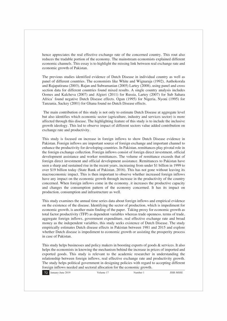
STYLIZED FACTSThis study is about observing the relationship between Dutch Disease effects and factor productivity and other economic growth sectors contribution, which can be proxy for economic growth. Before exploring any relation, the study briefly explains some of economic facts about the Pakistan. This is all about importance of the study and relevance with economic growth. Figure 1 is about the trend of economic growth (GDPGR). The graph clearly shows the declining trend over a period during early and mid-nineteen’s (90s) and then after 2007. In the first phase from 1980-1992, GDPGR is increasing and during 1993, 1997 and 2001, record decline in the economic growth. It starts increasing up to some extent after 2001 and decreased again in 2008. This leads to explore the causes behind that decrease. One of the factor may be decreasing trend in productivity lead to decrease the economic growth. During 2002-2006, there was no political government and foreign inflows especially workers’ remittances were coming in the country. This may be due to increase in the level of government expenditure on the development projects, which increased the productivity as well. Nevertheless, the trend is again decreasing excluding the year before. One of the causes may be Dutch Disease effects.

Zingales methodology. The author also found that trade deficit and terms of trade caused problem in the economic growth process.

The above mentioned literature clearly showed that previous work is about Dutch disease evidence at an aggregate level and lesser is discussed on becoming impediment to economic growth. This study is the first for Pakistan which estimated three sector based evidence of Dutch disease and clearly states that industrial sector is more impacted through this disease.

Economic growth is the annual growth rate of gross domestic product. Pakistan’s economic growth was about 4.72 percent during 1981-2016. Eighties is the ideal period for economic growth (6.3%) whereas nineties and twenties remained below average growth. The decade from 1991-2000 is the worst period in Pakistan economic growth averaging at 3.9 percent. Currently GDP growth is increasing after reaching its minimum level (1.6%). The economic growth is continuously decreasing since mid-eighties. This was the period of structural adjustment in Pakistan and movement from fixed exchange rate to flexible exchange rate. One can ask a question by looking at the historical picture, what is the potential rate of growth for Pakistan? Although there is no consensus on it but I could say that this economy has the potential of at least 7-8% rate of growth as its maximum level. This potential is not utilized. This caused to explore the reasons or impediments to economic growth in Pakistan.

Figure 1: Trend of Economic Growth


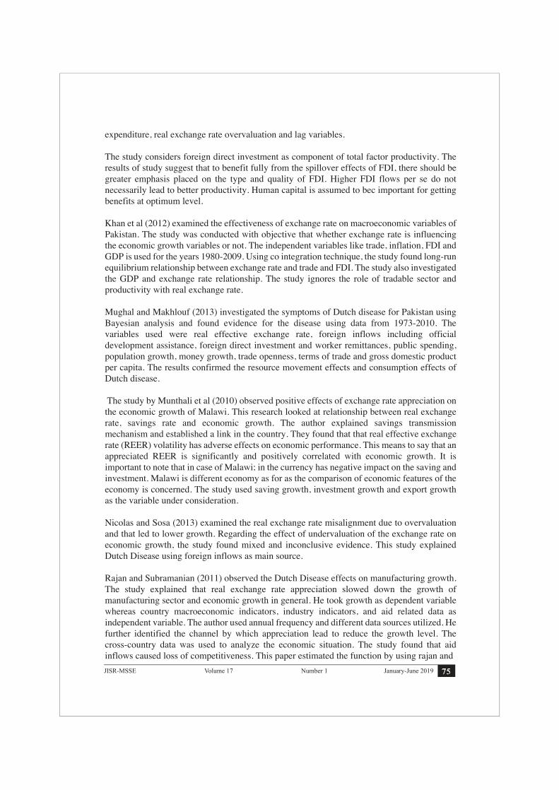
Foreign financial inflows play very important role in boosting the economic growth of developing as well as developed countries. The study considers three main types of inflows for Pakistan economy, workers’ remittances, foreign direct investment and net official development assistance coming abroad. On average, remittances were about 4 percent of GDP, foreign direct investment i.0 percent and official development assistance about 2.8 percent of GDP during 1981-2016. Current decade shows that remittances (REM) growth is tremendous at 8.8 percent of GDP. Similarly, during 2000s, official development assistance (ODA) and foreign direct investment (FDI) was about 2 percent of GDP. As for as the volatility is concerned, remittances showed higher variation compared to FDI and ODA during the same period. It is interesting to note that FDI, ODA and REM showed increasing trend during early eighties and now in second decade of the twentieth century. The early nineties period was not good for foreign inflows. Further to this it is to observe that when remittances are high the ODA and FDI showed decreasing trend during the same period of analysis.

This graph showed that gap between tradable and non-tradable sector is increasing. It is important to note that, agriculture and manufacturing are included in tradable goods sectors whereas construction, electricity, gas, water, and all types of services are under the category of non-tradable goods sector. Figure 3 shown shares of tradable goods and non-tradable goods to total output between 1981 and 2014. There is an obvious declining trend in tradable sector where it dropped from 45.93% in 1981 to 39.0% in 2014. Non-tradable goods sector, on the other side, shows an inclining trend from 1981(46.5%) to 2014(53.5%). Expansion of non-tradable goods sector and contraction of tradable good sectors lead us to investigate Dutch disease. In 2006, tradable sector was 36.2% and the services sector was at its peak about 56.3% of GDP.

Figure 2: Trend of Foreign Financial Inflows

Figure 3: Trend of Tradable and Non-Tradable Sector


Real effective exchange rate (REER) is the price ratio of domestic to foreign currency. It can be bilateral or multilateral. Bilateral is the price ratio of two trading countries whereas multilateral is the sum of price ratios of different countries. The study estimated the REER using internal and external determinants and collected the actual series from Haver software. After comparing both series, it can be deducted that reer is mix of appreciation and depreciation in Pakistan. Government expenditure, money spending, terms of trade, trade openness and foreign inflows is taken as the determinants of REER. The difference between the estimated or equilibrium exchange rate and the actual REER gives the misaligned REER, which is shown in figure 4. The figure explains during eighties, more episodes of devaluation and same pattern is observed in nineties. Since2000s and onwards, Pakistani REER appreciated. This signifies the role of increase in foreign financial inflows and the appreciation in REER (Dutch Disease).

Figure 3: Trend of Tradable and Non-Tradable Sector

Figure 4: Trend of Real Effective Exchange Rate

Figure 5: Trend of Sectoral Employment share


Total factor productivity is estimated using cob Douglas production function technique. The study assumed 40 percent share of capital and 60percent labor share. Depreciation is assumed 6% as according to literature. The growth in total factor productivity is calculated. The growth series gives an idea about decreasing trend during the whole period of analysis. The decade-wise analysis illustrates that TfP was relatively better in eighties than in rest of the periods. This fact also motivated to explore the reasons of low TFP in Pakistan. The study use TFP as proxy of economic growth that is again as per literature. The study would explore the relationship between TFP and REER misalignment. This would determine whether overvaluation lead to slow the economic growth or not.

Sectoral employment explains the resource movement effect in Pakistan economic. It can easily be seen from figure 5 that agricultural sector employment decreased continuously whereas industrial employment level remained more or less the same and services sector employment increased significantly during the period of analysis. Agricultural sector employment was highest during eighties and services sector employment maximum is the current decade. Industrial sector employment that play key role in output growth remained stagnant. Industrial employment is below average and agriculture sector still show above average labor force.

Figure 6: Trend of Total Factor Productivity Growth (TFPG)

Figure 7: Trend of Terms of Trade in Pakistan


Figure 7 is about the trend of price ratio (price of exports to price of imports) in Pakistan. It can be easily seen that terms of trade are on declining trend. This means that export prices decreasing as compared to imports. This ratio actually directly affects the tradable and non-tradable sector. If the prices of exports are up to mark, domestic investor discouraged and contracts the output in the country of analysis and vice versa.

As the study is divided into two parts, first detecting appreciation in REER and then observe the appreciated REER role in assessing the hurdle in economic growth. The impact of Dutch Disease on economic growth in Pakistan can be examined using a model. The model is specified thus: REER = f (FDI, REM, ODA, M2 GCE, TROP)…………………………..…….1 TFP (economic growth) = f (FI, EXR, GCE, TROP, TOT) ……………….……2

TFP= α0 + β1FI + β2REER + β3GCE + β4TROP + β4TOT + μ………………3Equation 1 is the functional relation between total factor productivity as dependent variable and FI as foreign inflows that is the sum of the three different financial inflows. i.e., Remittances (REM), foreign direct investment (FDI), and Official development assistance (ODA). Equation 2 is the estimated relationship where βs are the coefficients. These

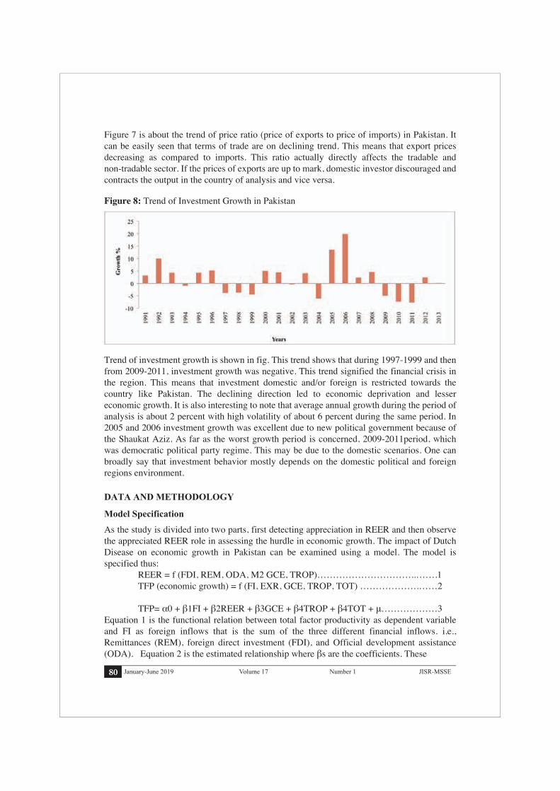
Trend of investment growth is shown in fig. This trend shows that during 1997-1999 and then from 2009-2011, investment growth was negative. This trend signified the financial crisis in the region. This means that investment domestic and/or foreign is restricted towards the country like Pakistan. The declining direction led to economic deprivation and lesser economic growth. It is also interesting to note that average annual growth during the period of analysis is about 2 percent with high volatility of about 6 percent during the same period. In 2005 and 2006 investment growth was excellent due to new political government because of the Shaukat Aziz. As far as the worst growth period is concerned, 2009-2011period, which was democratic political party regime. This may be due to the domestic scenarios. One can broadly say that investment behavior mostly depends on the domestic political and foreign regions environment.

Figure 8: Trend of Investment Growth in Pakistan

DATA AND METHODOLOGY

Model Specification


To arrive at estimating the total factor productivity for the economy as a whole, aggregate TFP is estimated using capital share of 40% and depreciation at 6%. The different sector wise TFP is also calculated using the agricultural, industrial, services sector value added, assuming capital share, and rate of depreciation as taken together case.

Total Factor Productivity (TFP)

The study took annual time series for three kinds of foreign inflows. This data is collected using the Have Analytic software. The reason for estimating different foreign inflows for tin the regression is to capture the different impact. Since there is also connotation among the economist about the usefulness of the foreign inflows. Some economist is of the view that foreign inflows play key role and rest of the economist denied this claim. The expected sign for the foreign inflows with TFP is positive.

Foreign Inflows (FI)

The annual time series for the real effective exchange rate and the nominal exchange rate is collected from the same source (Haver analytic). The increase in it is the depreciation and increase in REER is the appreciation. Appreciation in REER is causing the tradable sector to shrink, de-industrialization, and low per capita and hence low level of economic growth. The expected sign for the REER is negative.

Exchange Rate (REER)

Annual time series for the terms of trade is collected from the same source. It is the ratio of price of exports to price of imports. Increase in this ratio improvement in the TOT and vice versa. This has a positive expected relation with the TFP. Some economist argued that TOT has negative relation with TFP.

Terms of Trade (TOT)

This measure the amount government expends yearly on necessities and important socio-economic infrastructures such as roads, housing, electricity, water, etc. It has the impact in economic growth and productivity of the country concerned. It has theoretically positive relation with the TFP.

Government Expenditure

Trade openness is the ratio of sum of exports and imports to gross domestic product. This ratio expected relation with TFP would be positive. Since increase in the TROP may lead to increase in the output and productivity. The developed countries and developing countries have different experiences on this argument.

Trade Openness (TROP)

elaborate the behavior of the productivity due to independent variables, which provide guidelines in designing the policy for the economy like Pakistan.


This variable is constructed to using actual series for real effective exchange rate and the estimated for equilibrium exchange rate series. The difference between equilibrium and actual REER is the misalignment. The positive values or more increase in the actual series reduces the difference and showing decrease in reer hence the depreciation and vice versa. Appreciation in reer is the sign of Dutch disease effect. If it is causing TFP to decease hence, is impediment to economic growth and vice versa.

Misaligned REER (MISAL)

In this essay, time-series analysis is done to analyze the effects of real effective exchange rate (REER) and other control variables on total factor productivity (TFP) in Pakistan. The econometric methodology will be separated into two parts, where the first part is to examine the effect of foreign financial inflows on REER (spending effect) and the resources reallocation effect of Dutch disease by using sectoral analysis on the output of tradable and non-tradable sectors whereas the second part is to observe the aggregative as well as the sectoral impact of productivity (proxy for economic growth) with REER appreciation.

In the first part, Real Effective Exchange Rate (REER) will be used as the dependent variable. Then, observe how different foreign inflows and other variables (inflation rate (M2), Trade openness (TROP), terms of trade (TOT), government expenditure (GEXP) and foreign inflows (FI)) affect the dependent variable. The REER index is directly collected from the World Bank with the base year of year 2005. We then convert its base year into year 2000 for data consistency purpose.

For computing foreign inflows contribution in gross domestic product (GDP), foreign direct investment, official development assistance and remittances as a share of GDP is collected by dividing all the independent variables with the nominal GDP in constant USD. Both of the data are also adopted from world development indicators (WDI) of the World Bank. The data of labor and capital is collected from the handbook statistics for fifty years of Pakistan published by state bank to calculate the productivity of concerned period. For the sectoral estimations, this paper use value added data as a share of GDP for the agriculture, manufacturing and services sectors as the dependent variables (WDI database). Other variables are the trade openness (Trop), terms of trade (TOT), GDP per capita (GDPPC), GDP growth, money and quasi money (M2) and general government expenditure (GEXP).

Methodology

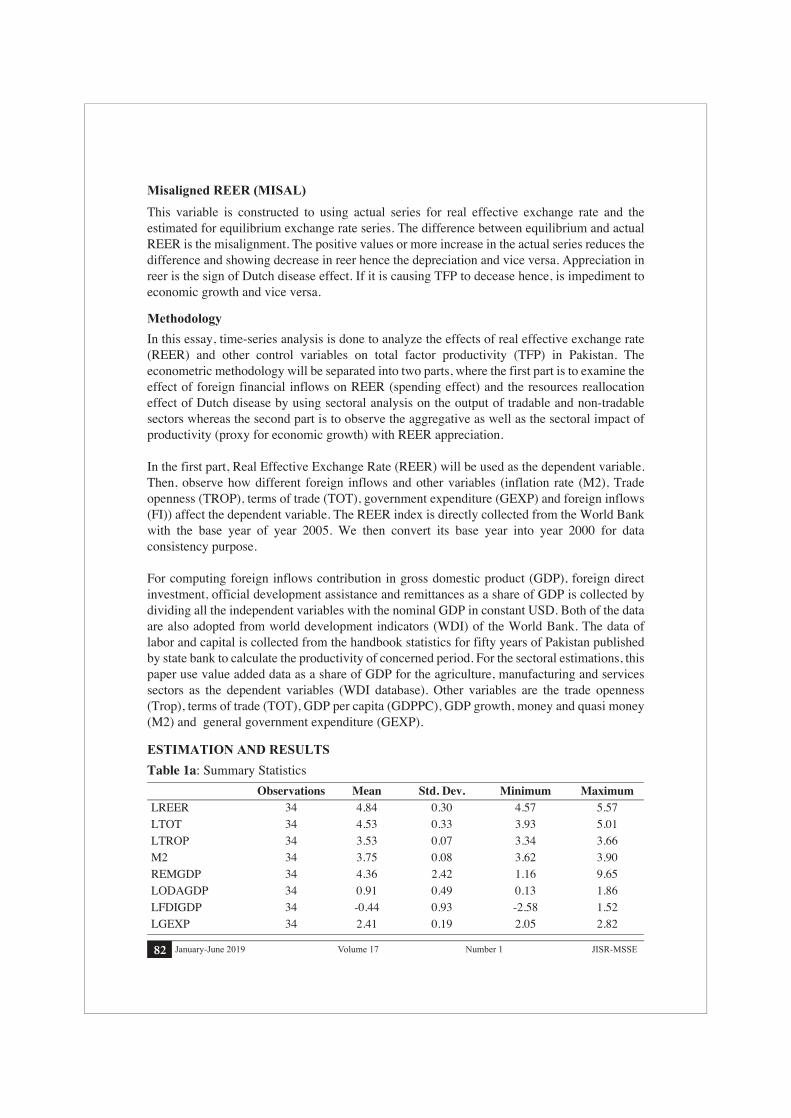
ESTIMATION AND RESULTSTable 1a: Summary Statistics Observations Mean Std. Dev. Minimum MaximumLREER 34 4.84 0.30 4.57 5.57LTOT 34 4.53 0.33 3.93 5.01LTROP 34 3.53 0.07 3.34 3.66M2 34 3.75 0.08 3.62 3.90REMGDP 34 4.36 2.42 1.16 9.65LODAGDP 34 0.91 0.49 0.13 1.86LFDIGDP 34 -0.44 0.93 -2.58 1.52LGEXP 34 2.41 0.19 2.05 2.82


Table 1b: Correlations LREER LM2 LGEXP LREMGDP LTOT LTROP LFDIGDP LODAGDPLREER LM2 -0.25 LGEXP 0.38 -0.20 LREMGDP 0.31 -0.28 0.10 LTOT 0.60 0.18 0.42 -0.45 LTROP 0.19 0.23 0.64 -0.03 0.30 LFDIGDP -0.76 0.34 -0.36 -0.06 -0.66 0.01 LODAGDP 0.79 -0.35 0.36 0.24 0.45 0.14 -0.63

Table 2: Unit Root Tests ADF- Level (Prob) ADF-Ist Difference (Prob) Constant Constant & trend Constant T-stat Prob T-stat Prob T-stat ProbFDI -1.44 0.55 -3.66 0.04 -4.81 0.00REM -0.63 0.85 -0.72 0.96 -4.24 0.00ODA -2.66 0.09 -3.79 0.03 -6.92 0.00REER -4.01 0.00 -1.14 0.91 -3.46 0.02TOT -0.14 0.94 -2.41 0.37 -5.05 0.00TROP -2.79 0.07 -3.05 0.13 -8.61 0.00GEXP -1.37 0.59 -1.66 0.75 -4.76 0.00M2 -2.72 0.08 -2.61 0.28 -5.21 0.00

Table 1b, is the cross correlations, illustrates the strength of relationship among different variables. This gives an idea whether regressions and co integration workable or not. If the strength of correlations is more than 60 percent then may cause multicollinearity and endogeneity problem in the analysis. Since the main objective of the study is to establish the Dutch disease and prove it as impediment to economic growth. REER worked as dependent variable and rest of the variables as explanatory. TROP shows low correlation with the REER and rest of the variables has very strong relationship. Foreign inflow and M2 showed negative cross correlation. Again, this negative relationship gives a clue to investigate the Dutch disease effects on economic growth.

This table 1a explained the descriptive statistics among different variables. Summary statistics help in understanding the problem discussed and finding trends of the variables of interest. The data set consists of 34 observations (column 1). Column 2 is about the average values of the variables. REER, TOT and REM have the largest mean value and ODA & FDI have smallest mean value. Similarly, standard deviation of of TOT, TROP and Government expenditure is lowest during the same period. The standard deviation explains the distance from target value. FDI and REM obtain the maximum distance in terms of standard deviation. Column 3 and column 4 are about the range of the variables movements. It is interesting to note that foreign financial inflows contain largest ranges whereas M2 and TROP have smallest ranges over the same period of analysis. The summary statistics gives an overview about the raw data, the direction and the magnitude of their variations. This helps in identify which variable is to transform and up to what extent its transformation worked.


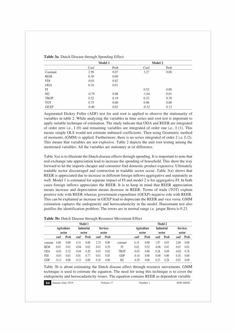
Table 3b: Dutch Disease through Resource Movement Effect Model 1 Model 2 Agriculture Industrial Services Agriculture Industrial Services sector sector sector sector sector sector

constant 4.68 0.00 4.31 0.00 2.74 0.00 constant 6.15 0.00 1.97 0.03 2.68 0.00REM 0.03 0.01 -0.04 0.02 0.01 0.29 FI 0.02 0.52 -0.06 0.01 0.03 0.01ODA -0.03 0.32 -0.04 0.20 0.03 0.02 TROP -0.03 0.80 0.28 0.09 -0.02 0.76FDI -0.03 0.01 0.01 0.77 0.01 0.05 GDP -0.16 0.00 -0.08 0.00 0.10 0.00GDP -0.13 0.00 -0.13 0.00 0.10 0.00 M2 -0.29 0.06 0.23 0.28 0.03 0.69

Table 3a: Dutch Disease through Spending Effect Model 1 Model 2 Coef Prob Coef ProbConstant 2.99 0.07 3.27 0.08REM 0.30 0.00 FDI -0.01 0.82ODA 0.16 0.01FI 0.52 0.00M2 -0.79 0.08 -1.04 0.01TROP 0.52 0.19 0.32 0.39TOT 0.75 0.00 0.90 0.00GEXP -0.40 0.03 -0.32 0.12

coef Prob coef Prob coef Prob coef Prob coef Prob coef Prob

Table 3b is about estimating the Dutch disease effect through resource movements. GMM technique is used to estimate the equation. The need for using this technique is to cover the endogeneity and heroscadasticity issues. The equation contains REER as dependent variable

Augmented Dickey Fuller (ADF) test for unit root is applied to observe the stationarity of variables in table 2. While analyzing the variables in time series unit root test is important to apply suitable technique of estimation. The study indicate that ODA and REER are integrated of order zero i.e., I (0) and remaining variables are integrated of order one i.e., I (1). This means simple OLS would not estimate unbiased coefficients. Then using Geometric method of moments, (GMM) is applied. Furthermore, there is no series integrated of order 2 i.e. I (2). This means that variables are not explosive. Table 2 depicts the unit root testing among the mentioned variables. All the variables are stationary at ist difference.

Table 3(a) is to illustrate the Dutch disease effects through spending. It is important to note that real exchange rate appreciation lead to increase the spending of household. This show the way forward to let the imports cheaper and consumer find domestic product expensive. Ultimately tradable sector discouraged and contraction in tradable sector occur. Table 3(a) shows that REER is appreciated due to increase in different foreign inflows aggregative and separately as well. Model 1 is estimated for separate impact of FI and model 2 is for aggregative FI. In both cases foreign inflows appreciates the REER. It is to keep in mind that REER appreciation means increase and depreciation means decrease in REER. Terms of trade (TOT) explain positive role with REER whereas government expenditure (GEXP) negative role with REER. This can be explained as increase in GEXP lead to depreciate the REER and vice versa. GMM estimation captures the endogeneity and heroscadasticity in the model. Haussmann test also justifies the identification problem. The errors are in normal range i.e. jarque Berra is 0.23.


Table 4: From Overvaluation to TFP Growth. Model 1 Model 2 coef Prob coef ProbConstant 0.30 0.00 0.319 0.000REM -0.01 0.01 FDI 0.00 0.41 ODA -0.01 0.00 FI -0.002 0.656M2 0.05 0.03 -1.042 0.011TROP 0.00 0.99 0.055 0.065TOT -0.05 0.00 -0.032 0.002REER -0.03 0.00 -0.037 0.001GEXP 0.02 0.13 -0.013 0.282

3- See appendix for VAR analysis and tables. In addition, estimations by taking Growth rate as dependent variable using VAR model technique.

After detecting the Dutch Disease in Pakistan, the study focus is on explaining the channel of total factor productivity (TFP) in economic growth. The series for total factor productivity has been estimated and its graph is explained in the stylized facts. The study investigates the link between real exchange rate overvaluation and TFP. The determinants of TFP are TROP, M2, human capital, financial inflows proxies as REM, ODA, FDI, and foreign prices (Edwards, 1998). Since the variables of the study create endogeneity among variables so, the GMM estimation technique proposed by Blundell and Bond (1998) is used to endogeneity and identification of causal relation from overvaluation to TFP.

Table 4, present the results of equation of factor productivity considering TROP, TOT, REER, and foreign inflows as independent variables. Real effective exchange rate coefficient is negative and significant with TFP. Remittances and official development assistance coefficient is significant and negative, showing increase in inflows decrease the TFP of Pakistan economy. Hence, it is justified that Dutch disease may be considered as an impediment to economic growth.

and the explanatory variables like foreign financial inflows, GDP, TROP and M2. Model 1 is about sector impact of different foreign inflows and GDP variables. The negative coefficient of REM on industrial sector shows contracting the tradable sector and positive coefficient for services and agriculture depicts expansion in the non-tradable sector. Model 2 is about estimating the sectoral impact taking foreign inflows as aggregate (FI). Again, FI shows negative coefficient for industrial sector and positive for the other two sectors. Since it has already been established that REER is appreciated in Pakistan during the period of analysis, as a second step it is easily comprehended that its impact in the industrial which is the important part of tradable sector. Another important policy variable is to be noticed that GDP increase is going to decrease the industrial output and provide little jump to services sector output. Money supply on the other hand illustrate insignificant role in real sectors. The estimates consider the impact of foreign inflows on REER and then REER misalignment series. This can be observed that REER appreciation empirically showing negative relationship with TFP. This verifies the main hypothesis of the study as impediment to economic growth in Pakistan. The alternative methodology is also used to estimate the relationship for robustness check3.


4- For details see the appendix

Figure 6: Overvaluation and Growth Relationship

Table 5: Correlation between REER and Economic Growth Proxy (Sector-wiseTFP) MISAL TFPA TFPI TFPSMISAL 1.00 TFPA 0.09 1.00 TFPI -0.40 -0.41 1.00 TFPS 0.10 -0.35 -0.34 1.00

To check for robustness, the paper estimated TFP for three sectors of the economy, agriculture, industrial and services. TFPA stands for total factor productivity of agriculture sector, TFPI is the productivity of industrial sector and TFPS is the productivity of the services sector. Table 5 explained the correlation between the TFP of different sectors with the misaligned index estimated. It can be seen from this table that TFPI is negatively related to REER. This proved that appreciation in REER causing employment shift from agriculture or industrial sector to services sector. So the link between TFP and REER is established.

Figure 6 depicts the graph for the relationship between the concerned variables. This can be observed that when undervaluation the TFP is positive during early nineties. During the mid-nineties appreciation episode combines the decreasing effect on TFP. In 2003-05, episodes of currency devaluation, leading TFP to grow positively and 2006-09 appreciation leading to declining trend in productivity. Hence, the study established that there is strong negative relationship between overvaluation and economic growth.

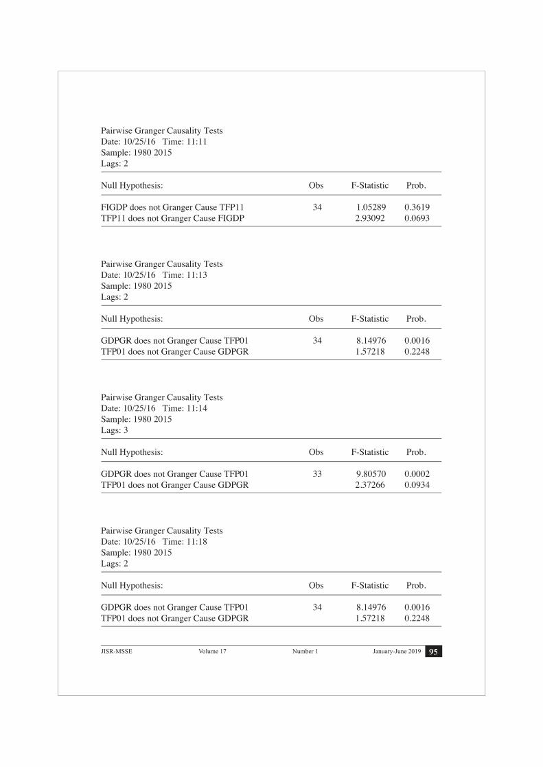
Further to test the long run relationship and identifying the direction of causality among variables, Granger causality test4 is applied. The Granger (1969) approach helped the researcher to observe the direction of the current explained by past values by adding lagged values. If the t-statistics is significant at 5 percent or 10 percent may then the prediction the variables are expected to be related with in specific direction. The two-way causation would exist when we accept both the null hypothesis, it is important to note that variables having significant granger relationship may not have the causation.

Table in appendix shows that TFP has one direction causality that is TFP does granger cause the economic growth. Similarly, exchange rate has two-way causation with TFP. This means that increase in TFP is based on past values. The other variables TROP Govt expenditure and credit to private sector have also have rejected the null hypothesis and two way causation exists among these variables.


CONCLUDING REMARKSThe study was carried out to examine the impact of Dutch Disease effects on the total factor productivity and economic growth of Pakistan. TFP is taken as dependent variable and proxy for the economic growth. The method of analysis adopted is GMM estimation technique in the E-Views software. The estimated results reveal a negative long run relationship between REER and productivity.This goes against the belief about the positive relationship between the two variables. Hence worked as the violation of the expectation between REER and TFP occurs because of appreciation in exchange rate.

The study is to first detect the Dutch disease effects in Pakistan. Secondly, explore the missing link of this misaligned REER causing Dutch Disease with economic growth and total factor productivity. The study confirms the evidence of Dutch disease effects and existence of low productivity as a link for hindrance economic growth. This productivity channel verifies the growth-reducing effect of overvaluation is in industrial sector. The study highlighted sectoral growth impact on employment due to increase in foreign financial inflows. In light of the conclusions, policy makers need to receive ODA, FDI, and REM with a caution of utilizing for production purposes instead consumption. If the economy is in appreciation state then foreign inflows need to be controlled or otherwise enhance foreign inflows in case of depreciation. It is suggested that mechanism should be developed to stabilize the appreciation depreciation in real effective exchange rate. The Pakistan government and the central bank has an important role to play in providing essential framework for controlling the exchange rate fluctuations. The following are important suggestions:

a. The study identified that role of remittances in agriculture sector, and ODA & FDI in the industrial sector is important to address.

b. To improve the depressing growth rate and productivity, there must be stable, economic friendly environment in the country.

c. To stabilize the exchange rate in order to improve the productivity in industrial sector and economic growth, moderate monetary policy, control on sudden stops in foreign inflows, targeting inflation at bearable level, control on budget deficit and current account deficit are the major actions. d Also, government expenditures must be directed towards productive economic activities such as building of power infrastructure, constructing economic corridors, and ensuring sufficient oil and water to reduce the cost of production.

REFERENCESAghion, P.. Bacchetta.P., Ranciere.R and Rogoff. K.. (2009). ‘Exchange Rate Volatility and

Productivity Growth: The Role of Financial Development,’ Journal of Monetary Economics, Vol. 56, pp.494-513.

Attah-Obeng., Enu, P., and Opoku.C. (2013). ‘An Econometric Analysis of the Relationship between GDP Growth Rate and Exchange Rate in Ghana’, Journal of Economics and Sustainable Development Vol.4, No.9, pp. 9-17.

Algieri.B. (2011).’The Dutch Disease: Evidences from Russia’, Econ Change Restruct,Vol. 44, pp. 243–277

Athukorala,P.and Rjapatirana. S (2003).’Capital Inflows and the Real Exchange Rate: A Comparative Study of Asia and Latin America’. The World Economy. Vol. 26, pp. 613-637.


Athukorala, P. and Warr. P (2002). ‘’Vulnerability to a Currency Crisis and Recovery: Lessons from the Asian Experience,’ The World Economy.Vol. 25, pp. 33-57.

Azid.T, Jamil.M, and Kousar.A. (2005) ‘Impact of Exchange Rate Volatility on Growth and Economic Performance: A Case Study of Pakistan, 1973–2003’, Pakistan Development Review Vol. 44:No. 4 ,pp. 749–775.

Baum, C. F. and Schaffer.M.E (2002). ‘Instrumental Variables and GMM: Estimation and Testing. Boston College Economic Working Paper No. 545.

Botta. A, Godin.A, and Messalina.M, (2015) ‘Finance, Foreign Direct Investment, and Dutch Disease: The Case of Colombia,’ Working Paper No. 853

Botta. A (2014).’The Macroeconomics of a Financial Dutch Disease,’.Post Keynesian Study Groiup Working Paper 1410.

Brahmbhtt.M Caunto.O and Ekatarioca.V (2010) ‘ Dealing with Dutch Disease, The world Bank issue 16, pp.1-7.

Cakrani.E. (2015). ‘Factors that effect Real Exchange Rate: Case of Albania,’ Euro Economica, issue.2, pp. 93-100.

Cordon, M. andNeary.J.P 1982. ‘Booming Sector and De-industrialization in Small Open Economy,’The Economic Journal, Vol. 92:, pp.825-848.

Gala.P. 2008. ‘Real exchange rate levels and economic development: theoretical analysis and econometric evidence’, Cambridge Journal of Economics, Vol.32, pp.273–288.

Khan.E. Sattar.R., Rehman.H. (2012) ‘Effectiveness of Exchange Rate in Pakistan: Causality Analysis Pak. Journal of. Commer. Soc. Sci. Vol. 6 ,No.1,pp. 83-96.

Lartey.K.(2007)’Capital inflows and real exchange rate, an empirical evidence of Sub Sahara Africa’, The Journal of international trade and economic development,Vol. 16, pp. 337-357.

Lartey.K (2008) ‘Capital inflows, Dutch Disease effects and monetary policy in small open economy, Review of international economics, Vol.20, issue 2, pp. 34-44.

Magud.N and Sosa. S. (2013), When and Why worry about Real Exchange Rate appreciation, the missing link between Dutch Disease and Growth, Journal of International commerce, economics and policy, Vol.04, No. 02.

Makhlouf. F and Mughal.M. (2013). ‘Remittances, Dutch Disease, and Competitiveness: A Baysian Analysis, Journal of Economic Development Vol 38,No.2, pp. 67-97.

Munthali.T, Simwaka.K and Mwale.M. (2010) ‘ The real exchange rate and economic growth in Malawi: exploring transmission route’, Journal of development and agricultural economics, Vol. 2, No.9, pp. 303-315.

Nyoni.O. (1995) ‘Foreign aid and economic performance in Tanzania, World Development, Vol. 26, No. 7, pp. 1235-1240.

Ogun.O. (1995) ‘Real Exchange rate movements and export growth in Nigeria, 1960-90’, African Research Consortium, Research Paper No.82.

Omes.N and Kelcheva.K. (2007) ‘Diagniosing Dutch Disease, Does Russia have the symptom,’ International Monetary Fund, Working Paper No. wp/07/102.

Rajan.R and Subramanium.A (2011) ‘Aid, Dutch Disease and manufacturing growth’, Journal of development economics, Vol. 94, No. 1, pp. 106-118.

Sackey.H.A. (2001) ‘External aid flow and real exchange rate in Ghana, African Economic Research Consortium, Research Paper No. 110.

White.H., and Wignaraja.G (1992) ’Exchange rate, Trade liberalization and aid’, World Development, Vol. 20, pp. 1471-1480.


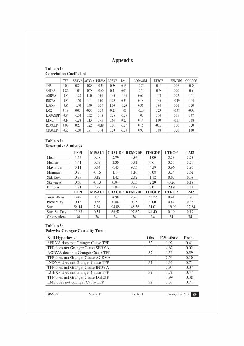
AppendixTable A1:Correlation Coefficient

Table A2:Descriptive Statistics

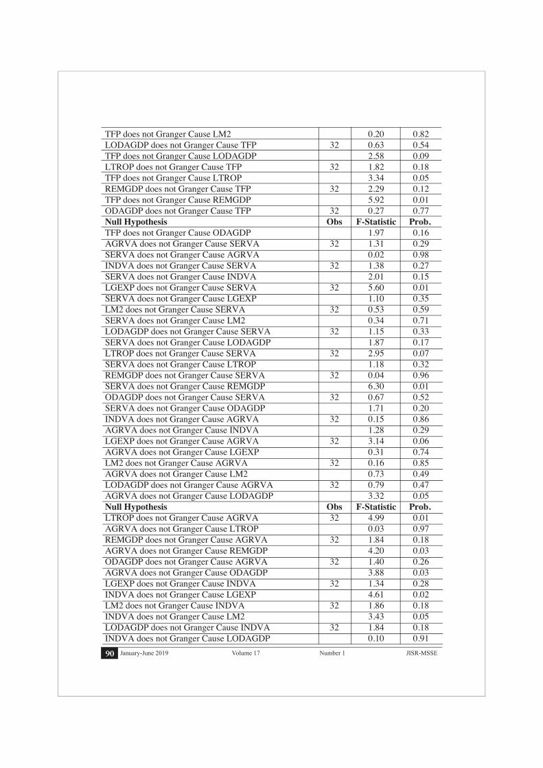
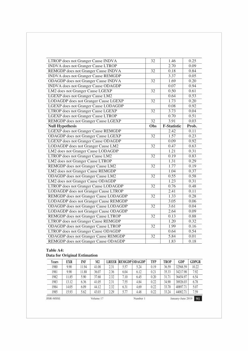
Table A3:Pairwise Granger Causality Tests

Null Hypothesis Obs F-Statistic Prob. SERVA does not Granger Cause TFP 32 0.92 0.41 TFP does not Granger Cause SERVA 4.62 0.02 AGRVA does not Granger Cause TFP 32 0.55 0.59 TFP does not Granger Cause AGRVA 2.51 0.10 INDVA does not Granger Cause TFP 32 0.35 0.71 TFP does not Granger Cause INDVA 2.97 0.07 LGEXP does not Granger Cause TFP 32 0.78 0.47 TFP does not Granger Cause LGEXP 0.99 0.38 LM2 does not Granger Cause TFP 32 0.31 0.74

TFP SERVA AGRVA INDVA LGEXP LM2 LODAGDP LTROP REMGDP ODAGDPTFP 1.00 0.84 -0.83 -0.33 -0.38 0.19 -0.77 -0.14 0.08 -0.83SERVA 0.84 1.00 -0.78 -0.60 -0.40 0.07 -0.54 -0.28 0.20 -0.60AGRVA -0.83 -0.78 1.00 0.01 0.40 -0.35 0.62 0.13 0.22 0.71INDVA -0.33 -0.60 0.01 1.00 0.29 0.33 0.18 0.45 -0.49 0.14LGEXP -0.38 -0.40 0.40 0.29 1.00 -0.20 0.36 0.64 0.01 0.30LM2 0.19 0.07 -0.35 0.33 -0.20 1.00 -0.35 0.23 -0.37 -0.38LODAGDP -0.77 -0.54 0.62 0.18 0.36 -0.35 1.00 0.14 0.15 0.97LTROP -0.14 -0.28 0.13 0.45 0.64 0.23 0.14 1.00 -0.17 0.08REMGDP 0.08 0.20 0.22 -0.49 0.01 -0.37 0.15 -0.17 1.00 0.20ODAGDP -0.83 -0.60 0.71 0.14 0.30 -0.38 0.97 0.08 0.20 1.00

TFP1 MISAL1 ODAGDP REMGDP FDIGDP LTROP LM2 Mean 1.65 0.08 2.79 4.36 1.00 3.53 3.75 Median 1.41 0.09 2.30 3.72 0.61 3.53 3.76 Maximum 3.11 0.34 6.45 9.65 4.59 3.66 3.90 Minimum 0.76 -0.15 1.14 1.16 0.08 3.34 3.62 Std. Dev. 0.78 0.12 1.42 2.42 1.12 0.07 0.08 Skewness 0.50 -0.13 0.94 0.65 2.20 -0.26 0.18 Kurtosis 1.81 2.28 3.04 2.47 7.01 2.89 1.81 TFP1 MISAL1 ODAGDP REMGDP FDIGDP LTROP LM2Jarque-Bera 3.42 0.82 4.98 2.76 50.22 0.41 2.20 Probability 0.18 0.66 0.08 0.25 0.00 0.82 0.33 Sum 56.14 2.64 94.88 148.36 34.01 119.90 127.64 Sum Sq. Dev. 19.83 0.51 66.52 192.62 41.40 0.19 0.19 Observations 34 34 34 34 34 34 34


TFP does not Granger Cause LM2 0.20 0.82 LODAGDP does not Granger Cause TFP 32 0.63 0.54 TFP does not Granger Cause LODAGDP 2.58 0.09 LTROP does not Granger Cause TFP 32 1.82 0.18 TFP does not Granger Cause LTROP 3.34 0.05 REMGDP does not Granger Cause TFP 32 2.29 0.12 TFP does not Granger Cause REMGDP 5.92 0.01 ODAGDP does not Granger Cause TFP 32 0.27 0.77 Null Hypothesis Obs F-Statistic Prob. TFP does not Granger Cause ODAGDP 1.97 0.16 AGRVA does not Granger Cause SERVA 32 1.31 0.29 SERVA does not Granger Cause AGRVA 0.02 0.98 INDVA does not Granger Cause SERVA 32 1.38 0.27 SERVA does not Granger Cause INDVA 2.01 0.15 LGEXP does not Granger Cause SERVA 32 5.60 0.01 SERVA does not Granger Cause LGEXP 1.10 0.35 LM2 does not Granger Cause SERVA 32 0.53 0.59 SERVA does not Granger Cause LM2 0.34 0.71 LODAGDP does not Granger Cause SERVA 32 1.15 0.33 SERVA does not Granger Cause LODAGDP 1.87 0.17 LTROP does not Granger Cause SERVA 32 2.95 0.07 SERVA does not Granger Cause LTROP 1.18 0.32 REMGDP does not Granger Cause SERVA 32 0.04 0.96 SERVA does not Granger Cause REMGDP 6.30 0.01 ODAGDP does not Granger Cause SERVA 32 0.67 0.52 SERVA does not Granger Cause ODAGDP 1.71 0.20 INDVA does not Granger Cause AGRVA 32 0.15 0.86 AGRVA does not Granger Cause INDVA 1.28 0.29 LGEXP does not Granger Cause AGRVA 32 3.14 0.06 AGRVA does not Granger Cause LGEXP 0.31 0.74 LM2 does not Granger Cause AGRVA 32 0.16 0.85 AGRVA does not Granger Cause LM2 0.73 0.49 LODAGDP does not Granger Cause AGRVA 32 0.79 0.47 AGRVA does not Granger Cause LODAGDP 3.32 0.05 Null Hypothesis Obs F-Statistic Prob. LTROP does not Granger Cause AGRVA 32 4.99 0.01 AGRVA does not Granger Cause LTROP 0.03 0.97 REMGDP does not Granger Cause AGRVA 32 1.84 0.18 AGRVA does not Granger Cause REMGDP 4.20 0.03 ODAGDP does not Granger Cause AGRVA 32 1.40 0.26 AGRVA does not Granger Cause ODAGDP 3.88 0.03 LGEXP does not Granger Cause INDVA 32 1.34 0.28 INDVA does not Granger Cause LGEXP 4.61 0.02 LM2 does not Granger Cause INDVA 32 1.86 0.18 INDVA does not Granger Cause LM2 3.43 0.05 LODAGDP does not Granger Cause INDVA 32 1.84 0.18 INDVA does not Granger Cause LODAGDP 0.10 0.91


1986 16.65 3.51 47.43 2.20 5.27 4.15 0.22 34.57 46423.59 5.50 1987 17.40 4.68 42.78 2.15 4.41 3.08 0.22 34.24 49419.00 6.45 1988 18.00 8.84 44.02 2.14 3.52 4.31 0.23 35.26 53187.33 7.63 1989 20.54 7.84 45.20 2.11 3.61 4.37 0.23 35.63 55825.30 4.96 1990 21.71 9.05 43.46 2.08 3.44 3.06 0.23 38.91 58314.32 4.46 1991 23.80 11.79 46.76 2.07 2.53 3.56 0.25 35.56 61265.94 5.06 1992 25.08 9.51 51.31 2.07 2.39 2.26 0.25 37.89 65987.03 7.71 1993 28.11 9.97 47.20 2.06 2.15 2.30 0.25 38.75 67146.92 1.76 1994 30.57 12.37 35.90 2.06 2.51 3.17 0.25 35.33 69656.48 3.74 1995 31.64 12.34 33.67 2.06 2.74 1.38 0.25 36.13 73113.25 4.96 1996 36.08 10.37 37.84 2.04 2.23 1.77 0.26 38.33 76656.75 4.85 1997 41.11 11.38 39.36 2.05 1.66 1.71 0.25 36.85 77434.35 1.01 1998 45.05 6.23 40.03 2.06 2.15 1.94 0.24 34.01 79409.11 2.55 1999 49.50 4.14 43.11 2.02 1.42 1.26 0.24 32.32 82315.59 3.66 2000 53.65 4.37 41.50 2.01 1.16 1.14 0.25 28.13 85822.30 4.26 2001 61.93 3.15 39.02 1.97 1.23 3.19 0.25 30.37 87523.72 1.98 2002 59.72 3.29 40.79 1.99 1.62 3.44 0.25 30.54 90345.86 3.22 2003 57.75 2.91 43.88 1.97 3.75 1.49 0.25 32.84 94724.31 4.85 Years EXR INF M2 LREER REMGDP ODAGDP TFP TROP GDP GDPGR 2004 58.26 7.45 39.85 1.97 3.90 1.72 0.26 30.30 101704.14 7.37 2005 59.51 9.06 40.66 1.99 3.60 1.78 0.28 35.25 109502.10 7.67 2006 60.27 7.92 43.31 2.00 3.68 2.18 0.27 35.68 116266.64 6.18 2007 60.74 7.60 45.31 1.99 4.20 1.98 0.28 32.99 121885.60 4.83 2008 70.41 20.29 41.37 1.98 4.84 1.27 0.27 35.59 123959.36 1.70 2009 81.71 13.65 38.98 1.98 5.52 2.30 0.27 32.07 127469.47 2.83 2010 85.19 13.88 39.14 2.00 6.73 2.43 0.26 32.87 129517.50 1.61 2011 86.34 11.92 39.19 2.01 7.28 2.62 0.27 32.94 133125.78 2.75 2012 93.40 9.69 42.75 2.02 8.86 1.46 0.27 32.81 138471.99 3.51 2013 101.63 7.69 45.66 2.01 9.54 1.49 0.28 33.34 146876.62 4.37 2014 101.10 7.19 45.76 2.04 9.65 1.50 0.28 31.00 151600.10 4.74 2015 102.77 2.54 43.57 2.08 9.53 0.94 0.30 28.05 157293.21 5.54

Years EXR INF M2 LREER REMGDP ODAGDP TFP TROP GDP GDPGR 1980 9.90 11.94 41.08 2.31 5.57 5.24 0.19 36.59 32568.59 10.22 1981 9.90 11.88 36.07 2.36 6.04 6.12 0.21 35.33 34217.98 7.92 1982 11.85 5.90 37.68 2.32 7.10 6.45 0.20 31.71 36454.97 6.54 1983 13.12 6.36 41.05 2.31 7.55 4.84 0.22 34.90 38926.03 6.78 1984 14.05 6.09 44.12 2.32 6.31 4.69 0.22 33.70 40897.71 5.07 1985 15.93 5.62 43.03 2.29 5.77 4.48 0.22 33.24 44002.71 7.59

LTROP does not Granger Cause INDVA 32 1.46 0.25 INDVA does not Granger Cause LTROP 2.70 0.09 REMGDP does not Granger Cause INDVA 32 0.18 0.84 INDVA does not Granger Cause REMGDP 3.37 0.05 ODAGDP does not Granger Cause INDVA 32 1.69 0.20 INDVA does not Granger Cause ODAGDP 0.07 0.94 LM2 does not Granger Cause LGEXP 32 0.50 0.61 LGEXP does not Granger Cause LM2 0.64 0.53 LODAGDP does not Granger Cause LGEXP 32 1.73 0.20 LGEXP does not Granger Cause LODAGDP 0.08 0.92 LTROP does not Granger Cause LGEXP 32 3.73 0.04 LGEXP does not Granger Cause LTROP 0.70 0.51 REMGDP does not Granger Cause LGEXP 32 3.91 0.03 Null Hypothesis Obs F-Statistic Prob. LGEXP does not Granger Cause REMGDP 2.42 0.11 ODAGDP does not Granger Cause LGEXP 32 1.57 0.23 LGEXP does not Granger Cause ODAGDP 0.09 0.92 LODAGDP does not Granger Cause LM2 32 0.47 0.63 LM2 does not Granger Cause LODAGDP 1.21 0.31 LTROP does not Granger Cause LM2 32 0.19 0.83 LM2 does not Granger Cause LTROP 1.31 0.29 REMGDP does not Granger Cause LM2 32 1.77 0.19 LM2 does not Granger Cause REMGDP 1.04 0.37 ODAGDP does not Granger Cause LM2 32 0.55 0.58 LM2 does not Granger Cause ODAGDP 1.23 0.31 LTROP does not Granger Cause LODAGDP 32 0.76 0.48 LODAGDP does not Granger Cause LTROP 2.41 0.11 REMGDP does not Granger Cause LODAGDP 32 1.33 0.28 LODAGDP does not Granger Cause REMGDP 3.05 0.06 ODAGDP does not Granger Cause LODAGDP 32 3.61 0.04 LODAGDP does not Granger Cause ODAGDP 2.64 0.09 REMGDP does not Granger Cause LTROP 32 0.13 0.88 LTROP does not Granger Cause REMGDP 1.20 0.32 ODAGDP does not Granger Cause LTROP 32 1.99 0.16 LTROP does not Granger Cause ODAGDP 0.64 0.54 ODAGDP does not Granger Cause REMGDP 32 5.84 0.01 REMGDP does not Granger Cause ODAGDP 1.83 0.18

Table A4:Data for Original Estimation


1986 16.65 3.51 47.43 2.20 5.27 4.15 0.22 34.57 46423.59 5.50 1987 17.40 4.68 42.78 2.15 4.41 3.08 0.22 34.24 49419.00 6.45 1988 18.00 8.84 44.02 2.14 3.52 4.31 0.23 35.26 53187.33 7.63 1989 20.54 7.84 45.20 2.11 3.61 4.37 0.23 35.63 55825.30 4.96 1990 21.71 9.05 43.46 2.08 3.44 3.06 0.23 38.91 58314.32 4.46 1991 23.80 11.79 46.76 2.07 2.53 3.56 0.25 35.56 61265.94 5.06 1992 25.08 9.51 51.31 2.07 2.39 2.26 0.25 37.89 65987.03 7.71 1993 28.11 9.97 47.20 2.06 2.15 2.30 0.25 38.75 67146.92 1.76 1994 30.57 12.37 35.90 2.06 2.51 3.17 0.25 35.33 69656.48 3.74 1995 31.64 12.34 33.67 2.06 2.74 1.38 0.25 36.13 73113.25 4.96 1996 36.08 10.37 37.84 2.04 2.23 1.77 0.26 38.33 76656.75 4.85 1997 41.11 11.38 39.36 2.05 1.66 1.71 0.25 36.85 77434.35 1.01 1998 45.05 6.23 40.03 2.06 2.15 1.94 0.24 34.01 79409.11 2.55 1999 49.50 4.14 43.11 2.02 1.42 1.26 0.24 32.32 82315.59 3.66 2000 53.65 4.37 41.50 2.01 1.16 1.14 0.25 28.13 85822.30 4.26 2001 61.93 3.15 39.02 1.97 1.23 3.19 0.25 30.37 87523.72 1.98 2002 59.72 3.29 40.79 1.99 1.62 3.44 0.25 30.54 90345.86 3.22 2003 57.75 2.91 43.88 1.97 3.75 1.49 0.25 32.84 94724.31 4.85 Years EXR INF M2 LREER REMGDP ODAGDP TFP TROP GDP GDPGR 2004 58.26 7.45 39.85 1.97 3.90 1.72 0.26 30.30 101704.14 7.37 2005 59.51 9.06 40.66 1.99 3.60 1.78 0.28 35.25 109502.10 7.67 2006 60.27 7.92 43.31 2.00 3.68 2.18 0.27 35.68 116266.64 6.18 2007 60.74 7.60 45.31 1.99 4.20 1.98 0.28 32.99 121885.60 4.83 2008 70.41 20.29 41.37 1.98 4.84 1.27 0.27 35.59 123959.36 1.70 2009 81.71 13.65 38.98 1.98 5.52 2.30 0.27 32.07 127469.47 2.83 2010 85.19 13.88 39.14 2.00 6.73 2.43 0.26 32.87 129517.50 1.61 2011 86.34 11.92 39.19 2.01 7.28 2.62 0.27 32.94 133125.78 2.75 2012 93.40 9.69 42.75 2.02 8.86 1.46 0.27 32.81 138471.99 3.51 2013 101.63 7.69 45.66 2.01 9.54 1.49 0.28 33.34 146876.62 4.37 2014 101.10 7.19 45.76 2.04 9.65 1.50 0.28 31.00 151600.10 4.74 2015 102.77 2.54 43.57 2.08 9.53 0.94 0.30 28.05 157293.21 5.54

Years EXR INF M2 LREER REMGDP ODAGDP TFP TROP GDP GDPGR 1980 9.90 11.94 41.08 2.31 5.57 5.24 0.19 36.59 32568.59 10.22 1981 9.90 11.88 36.07 2.36 6.04 6.12 0.21 35.33 34217.98 7.92 1982 11.85 5.90 37.68 2.32 7.10 6.45 0.20 31.71 36454.97 6.54 1983 13.12 6.36 41.05 2.31 7.55 4.84 0.22 34.90 38926.03 6.78 1984 14.05 6.09 44.12 2.32 6.31 4.69 0.22 33.70 40897.71 5.07 1985 15.93 5.62 43.03 2.29 5.77 4.48 0.22 33.24 44002.71 7.59

Source: World Development Indicators (WDI) World Bank (2015)

Table A5:Data on Sector-wise Value-Added Statistics Years AGRVA INDVA SERVA TROP GEXP 1980 29.52 24.92 45.56 36.59 10.04 1981 30.83 22.60 46.57 35.33 10.16 1982 31.56 22.26 46.18 31.71 10.34 1983 30.26 22.07 47.67 34.90 11.42 1984 27.92 22.71 49.38 33.70 12.09 1985 28.54 22.47 49.00 33.24 12.10 1986 27.62 23.35 49.03 34.57 12.76 1987 26.25 24.02 49.73 34.24 13.53 Years AGRVA INDVA SERVA TROP GEXP 1988 26.02 24.38 49.60 35.26 15.51 1989 26.95 23.89 49.16 35.63 16.79


TFP2 MISAL1 ODAGDP REMGDP FDIGDP LTROP LM21981 2.083 0.202 6.117 6.041 0.316 3.565 3.6641982 2.357 0.258 6.448 7.099 0.175 3.457 3.7081983 2.154 0.125 4.839 7.553 0.076 3.552 3.7811984 2.303 0.185 4.691 6.311 0.136 3.517 3.6851985 2.201 0.231 4.480 5.766 0.299 3.504 3.7051986 2.300 -0.148 4.155 5.269 0.228 3.543 3.7681987 1.896 -0.019 3.083 4.413 0.262 3.533 3.8141988 1.498 0.081 4.313 3.520 0.351 3.563 3.7221989 1.413 0.078 4.371 3.613 0.377 3.573 3.6631990 1.132 -0.075 3.063 3.440 0.421 3.661 3.6671991 0.906 0.140 3.558 2.528 0.422 3.571 3.6681992 0.896 0.098 2.255 2.385 0.510 3.635 3.7551993 0.960 0.134 2.301 2.153 0.519 3.657 3.8211994 0.922 0.113 3.174 2.511 0.604 3.565 3.8231995 0.766 -0.146 1.377 2.744 0.988 3.587 3.774

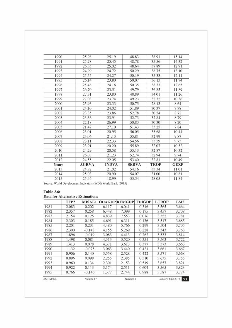
1990 25.98 25.19 48.83 38.91 15.14 1991 25.78 25.45 48.78 35.56 14.32 1992 26.35 25.02 48.64 37.89 12.91 1993 24.99 24.72 50.29 38.75 13.10 1994 25.55 24.27 50.19 35.33 12.11 1995 26.14 23.80 50.07 36.13 11.74 1996 25.48 24.16 50.35 38.33 12.65 1997 26.70 23.51 49.79 36.85 11.89 1998 27.31 23.80 48.89 34.01 11.26 1999 27.03 23.74 49.23 32.32 10.36 2000 25.93 23.33 50.75 28.13 8.64 2001 24.10 24.02 51.89 30.37 7.78 2002 23.35 23.86 52.78 30.54 8.72 2003 23.36 23.91 52.73 32.84 8.79 2004 22.18 26.99 50.83 30.30 8.20 2005 21.47 27.10 51.43 35.25 7.84 2006 23.01 20.95 56.05 35.68 10.44 2007 23.06 21.13 55.81 32.99 9.87 2008 23.11 22.33 54.56 35.59 9.75 2009 23.91 20.20 55.89 32.07 10.52 2010 24.29 20.58 55.13 32.87 10.32 2011 26.03 21.23 52.74 32.94 9.74 2012 24.55 22.05 53.40 32.81 10.49 Years AGRVA INDVA SERVA TROP GEXP 2013 24.82 21.02 54.16 33.34 11.01 2014 25.03 20.90 54.07 31.00 10.81 2015 25.46 18.99 55.54 28.05 11.84Source: World Development Indicators (WDI) World Bank (2015)

Table A6:Data for Alternative Estimations


1996 0.743 -0.078 1.774 2.233 1.203 3.646 3.8301997 0.742 0.137 1.715 1.658 0.925 3.607 3.875 TFP2 MISAL1 ODAGDP REMGDP FDIGDP LTROP LM21998 0.737 -0.046 1.936 2.150 0.637 3.527 3.8531999 0.838 0.176 1.261 1.424 0.646 3.476 3.8032000 0.529 0.341 1.138 1.161 0.359 3.337 3.6532001 0.340 0.090 3.186 1.228 0.438 3.413 3.6672002 0.008 0.204 3.438 1.617 0.911 3.419 3.7672003 0.084 -0.139 1.485 3.752 0.564 3.492 3.8382004 0.059 -0.021 1.717 3.898 1.099 3.411 3.8792005 0.082 -0.037 1.782 3.603 2.010 3.562 3.8962006 0.273 0.107 2.181 3.681 3.675 3.575 3.7972007 0.595 0.224 1.980 4.201 4.586 3.496 3.8592008 0.559 0.065 1.273 4.839 4.387 3.572 3.7742009 0.756 0.219 2.301 5.522 1.834 3.468 3.6962010 0.294 0.122 2.428 6.730 1.558 3.493 3.7172011 0.360 -0.004 2.616 7.279 0.983 3.495 3.6242012 0.204 -0.002 1.458 8.856 0.620 3.491 3.6892013 0.342 -0.052 1.489 9.536 0.890 3.501 3.7112014 0.192 0.077 1.500 9.648 1.007 3.439 3.690

Pairwise Granger Causality TestsDate: 10/25/16 Time: 11:09Sample: 1980 2015Lags: 2

Null Hypothesis: Obs F-Statistic Prob.

ODAGDP does not Granger Cause TFP01 34 3.04015 0.0633 TFP01 does not Granger Cause ODAGDP 2.89217 0.0716

Pairwise Granger Causality TestsDate: 10/25/16 Time: 11:11Sample: 1980 2015Lags: 2


LREER does not Granger Cause TFP11 34 3.92789 0.0309TFP11 does not Granger Cause LREER 2.20072 0.1289

Source: WDI & SBP


Pairwise Granger Causality TestsDate: 10/25/16 Time: 11:18Sample: 1980 2015 Lags: 2 Null Hypothesis: Obs F-Statistic Prob. GDPGR does not Granger Cause TFP01 34 8.14976 0.0016TFP01 does not Granger Cause GDPGR 1.57218 0.2248

Pairwise Granger Causality TestsDate: 10/25/16 Time: 11:11Sample: 1980 2015 Lags: 2


FIGDP does not Granger Cause TFP11 34 1.05289 0.3619TFP11 does not Granger Cause FIGDP 2.93092 0.0693

Pairwise Granger Causality TestsDate: 10/25/16 Time: 11:13Sample: 1980 2015 Lags: 2 Null Hypothesis: Obs F-Statistic Prob.

GDPGR does not Granger Cause TFP01 34 8.14976 0.0016TFP01 does not Granger Cause GDPGR 1.57218 0.2248

Pairwise Granger Causality TestsDate: 10/25/16 Time: 11:14Sample: 1980 2015 Lags: 3


GDPGR does not Granger Cause TFP01 33 9.80570 0.0002TFP01 does not Granger Cause GDPGR 2.37266 0.0934


REMGDP does not Granger Cause TFP01 34 0.31019 0.7357TFP01 does not Granger Cause REMGDP 1.13717 0.3346 ODAGDP does not Granger Cause TFP01 34 3.04015 0.0633TFP01 does not Granger Cause ODAGDP 2.89217 0.0716 BD does not Granger Cause TFP01 34 1.92133 0.1646TFP01 does not Granger Cause BD 1.48724 0.2427 GCEGDP does not Granger Cause TFP01 34 1.51062 0.2376TFP01 does not Granger Cause GCEGDP 1.97483 0.1570 LCPRS does not Granger Cause TFP01 34 0.37061 0.6935TFP01 does not Granger Cause LCPRS 1.22498 0.3085 REMGDP does not Granger Cause GDPGR 34 0.61409 0.5480GDPGR does not Granger Cause REMGDP 1.36816 0.2705 ODAGDP does not Granger Cause GDPGR 34 1.87474 0.1715GDPGR does not Granger Cause ODAGDP 3.30102 0.0511 BD does not Granger Cause GDPGR 34 0.14081 0.8692GDPGR does not Granger Cause BD 0.08937 0.9148 GCEGDP does not Granger Cause GDPGR 34 0.05892 0.9429GDPGR does not Granger Cause GCEGDP 2.72129 0.0826 LCPRS does not Granger Cause GDPGR 34 0.33791 0.7160GDPGR does not Granger Cause LCPRS 1.14918 0.3309 ODAGDP does not Granger Cause REMGDP 34 6.46218 0.0048REMGDP does not Granger Cause ODAGDP 0.74790 0.4823 BD does not Granger Cause REMGDP 34 0.16190 0.8513REMGDP does not Granger Cause BD 2.18940 0.1302 GCEGDP does not Granger Cause REMGDP 34 2.41117 0.1075REMGDP does not Granger Cause GCEGDP 3.28556 0.0517 LCPRS does not Granger Cause REMGDP 34 4.02853 0.0286REMGDP does not Granger Cause LCPRS 0.93464 0.4042 BD does not Granger Cause ODAGDP 34 0.15649 0.8559ODAGDP does not Granger Cause BD 1.01733 0.3741 GCEGDP does not Granger Cause ODAGDP 34 0.04978 0.9515ODAGDP does not Granger Cause GCEGDP 1.35156 0.2747


LCPRS does not Granger Cause ODAGDP 34 1.40375 0.2619ODAGDP does not Granger Cause LCPRS 1.32136 0.2824 GCEGDP does not Granger Cause BD 34 1.38818 0.2656BD does not Granger Cause GCEGDP 0.48546 0.6203 LCPRS does not Granger Cause BD 34 1.85507 0.1745BD does not Granger Cause LCPRS 2.00756 0.1526 LCPRS does not Granger Cause GCEGDP 34 0.10324 0.9022GCEGDP does not Granger Cause LCPRS 0.23453 0.7924 Null Hypothesis: Obs F-Statistic Prob. LREER does not Granger Cause TFP01 34 0.57342 0.5699TFP01 does not Granger Cause LREER 0.01526 0.9849


Documents

Dutch Disease as an impediment to Economic Growth of Pakistan