Embed Size (px)
Citation preview
Durham Research Online
Deposited in DRO:
15 June 2016
Version of attached �le:
Published Version
Peer-review status of attached �le:
Peer-reviewed
Citation for published item:
Lagos, C. D. P. and Theuns, T. and Schaye, J. and Furlong, M. and Bower, R. G. and Schaller, M. and Crain,R. A. and Trayford, J. W. and Matthee, J. (2016) 'The Fundamental Plane of star formation in galaxiesrevealed by the EAGLE hydrodynamical simulations.', Monthly notices of the Royal Astronomical Society.,459 (3). pp. 26323-32650.
Further information on publisher's website:
http://dx.doi.org/10.1093/mnras/stw717
Publisher's copyright statement:
This article has been accepted for publication in Monthly Notices of the Royal Astronomical Society c©: 2016 The
Authors Published by Oxford University Press on behalf of the Royal Astronomical Society. All rights reserved.
Additional information:
Use policy
The full-text may be used and/or reproduced, and given to third parties in any format or medium, without prior permission or charge, forpersonal research or study, educational, or not-for-pro�t purposes provided that:
• a full bibliographic reference is made to the original source
• a link is made to the metadata record in DRO
• the full-text is not changed in any way
The full-text must not be sold in any format or medium without the formal permission of the copyright holders.
Please consult the full DRO policy for further details.
Durham University Library, Stockton Road, Durham DH1 3LY, United KingdomTel : +44 (0)191 334 3042 | Fax : +44 (0)191 334 2971
http://dro.dur.ac.uk

MNRAS 459, 2632–2650 (2016) doi:10.1093/mnras/stw717Advance Access publication 2016 April 1
The Fundamental Plane of star formation in galaxies revealedby the EAGLE hydrodynamical simulations
Claudia del P. Lagos,1,2‹ Tom Theuns,3 Joop Schaye,4 Michelle Furlong,3
Richard G. Bower,3 Matthieu Schaller,3 Robert A. Crain,5 James W. Trayford3
and Jorryt Matthee4
1International Centre for Radio Astronomy Research (ICRAR), M468, University of Western Australia, 35 Stirling Hwy, Crawley, WA 6009, Australia2Australian Research Council Centre of Excellence for All-sky Astrophysics (CAASTRO), 44 Rosehill Street Redfern, NSW 2016, Australia3Institute for Computational Cosmology, Department of Physics, University of Durham, South Road, Durham DH1 3LE, UK4Leiden Observatory, Leiden University, PO Box 9513, NL-2300 RA Leiden, the Netherlands5Astrophysics Research Institute, Liverpool John Moores University, 146 Brownlow Hill, Liverpool L3 5RF, UK
Accepted 2016 March 23. Received 2016 March 22; in original form 2015 October 27
ABSTRACTWe investigate correlations between different physical properties of star-forming galaxies inthe ‘Evolution and Assembly of GaLaxies and their Environments’ (EAGLE) cosmologicalhydrodynamical simulation suite over the redshift range 0 ≤ z ≤ 4.5. A principal componentanalysis reveals that neutral gas fraction (fgas,neutral), stellar mass (Mstellar) and star formationrate (SFR) account for most of the variance seen in the population, with galaxies tracing a two-dimensional, nearly flat, surface in the three-dimensional space of fgas, neutral–Mstellar–SFR withlittle scatter. The location of this plane varies little with redshift, whereas galaxies themselvesmove along the plane as their fgas, neutral and SFR drop with redshift. The positions of galax-ies along the plane are highly correlated with gas metallicity. The metallicity can thereforebe robustly predicted from fgas, neutral, or from the Mstellar and SFR. We argue that the appear-ance of this ‘Fundamental Plane of star formation’ is a consequence of self-regulation, withthe plane’s curvature set by the dependence of the SFR on gas density and metallicity. Weanalyse a large compilation of observations spanning the redshift range 0 � z � 3, and findthat such a plane is also present in the data. The properties of the observed Fundamental Planeof star formation are in good agreement with EAGLE’s predictions.
Key words: stars: formation – ISM: evolution – galaxies: evolution – galaxies: formation –galaxies: ISM.
1 IN T RO D U C T I O N
The star formation rate (SFR) in a galaxy depends on the interplaybetween many physical processes, such as the rate at which thegalaxy’s halo accretes mass from the intergalactic medium, the rateof shocking and cooling of this gas on to the galaxy and the details ofhow a multiphase interstellar medium (ISM) converts gas into starsor launches it into a galactic fountain or outflow (see e.g. Benson &Bower 2010 and Somerville & Dave 2015 for recent reviews). Thecomplexity and non-linearity of these processes make it difficult tounderstand which processes dominate, and if and how this changesover time.
The identification of tight correlations between physical prop-erties of galaxies (‘scaling relations’) can be very valuable in re-ducing the apparent variety in galaxy properties, enabling the for-mulation of simple relations that capture the dominant paths along
� E-mail: [email protected]
which galaxies evolve. Recent efforts have been devoted to study-ing the SFR–stellar mass relation (e.g. Brinchmann et al. 2004;Noeske et al. 2007), stellar mass–gas metallicity relation (e.g.Tremonti et al. 2004; Lara-Lopez et al. 2010; Mannucci et al. 2010;Salim et al. 2014), and the stellar mass–gas fraction relation (e.g.Catinella et al. 2010; Saintonge et al. 2011). We begin by reviewingsome of these relations.
It has long been established that star-forming galaxies display atight correlation between SFR and stellar mass (Mstellar), and that thenormalization of this relation increases with redshift (z; e.g. Brinch-mann et al. 2004; Daddi et al. 2007; Noeske et al. 2007; Rodighieroet al. 2010). This ‘main sequence’ of star-forming galaxies has a1σ scatter of only ≈0.2 dex, making it one of the tightest knownscaling relations.
Lara-Lopez et al. (2010) and Mannucci et al. (2010) showed thatthe scatter in the Mstellar–gas metallicity (Zgas) relation (hereafter theMZ relation) is strongly correlated with the SFR, and that galaxiesin the redshift range z = 0 to z ≈ 2.5 populate a well-defined planein the three-dimensional space of Mstellar–Zgas–SFR. Mannucci et al.
C© 2016 The AuthorsPublished by Oxford University Press on behalf of the Royal Astronomical Society
at University of D
urham on June 15, 2016
http://mnras.oxfordjournals.org/
Dow
nloaded from
The fundamental plane of star formation 2633
(2010) noted that this relation evolves, breaking down at z � 3, withSalim et al. (2015) reporting even stronger evolution. The currentphysical interpretation of the MZ–SFR dependence is that whengalaxies accrete large quantities of gas, their SFR increases, andthe (mostly) low-metallicity accreted gas dilutes the metallicity ofthe ISM (e.g. Dave, Finlator & Oppenheimer 2012; De Rossi et al.2015). A corollary of this interpretation is that there should bea correlation between the scatter in the MZ relation and the gascontent of galaxies. Whether the residuals of the MZ relation aremore strongly correlated with the gas content than with the SFRwould depend on whether the gas metallicity is primarily set bythe dilution of the ISM due to accretion, or by the enrichment dueto recent star formation. In reality both should play an importantrole.
Hughes et al. (2013), Bothwell et al. (2013) and Lara-Lopez et al.(2013) show that the residuals of the MZ relation are also correlatedwith the atomic hydrogen (H I) content of galaxies, and that thescatter in the correlation with H I is smaller than in the correlationwith the SFR. Bothwell et al. (2016) extended the latter work toinclude molecular hydrogen (H2) and argue that the correlationbetween the residuals relative to the MZ fits are more stronglycorrelated with the H2 content than with the SFR of galaxies.
In parallel there have been extensive studies on the scaling re-lations between gas content, Mstellar and SFR. Local surveys suchas the Galex Arecibo SDSS Survey (GASS; Catinella et al. 2010),the CO Legacy Database for GASS (COLD GASS; Saintonge et al.2011), the Herschel Reference Survey (HRS; Boselli, Cortese & Bo-quien 2014a; Boselli et al. 2014b), the ATLAS3D (Cappellari et al.2011) and the APEX Low-redshift Legacy Survey for MOlecularGas (ALLSMOG; Bothwell et al. 2014), have allowed the explo-ration of the gas content of galaxies selected by Mstellar. Analysisof these data revealed that MH2/MH I correlates with Mstellar, andMH I/Mstellar anticorrelates with Mstellar (e.g. Catinella et al. 2010;Saintonge et al. 2011). Such local surveys also allow investigatinghow galaxy properties correlate with morphology: both MH I/Mstellar
and MH2/Mstellar decrease from irregulars and late-type galaxies toearly-type galaxies (Boselli et al. 2014b). In addition, the gas frac-tions decrease with increasing stellar mass surface density (Catinellaet al. 2010; Brown et al. 2015).
Surveys targeting star-forming galaxies at z > 0 allow one toinvestigate if z = 0 scaling relations persist, and how they evolve.The ratio MH2/Mstellar increases by a factor of ≈5 from z = 0 to2.5 at fixed Mstellar (e.g. Geach et al. 2011; Saintonge et al. 2011,2013; Tacconi et al. 2013; Bothwell et al. 2014; Santini et al. 2014;Dessauges-Zavadsky et al. 2015). Santini et al. (2014) presentedmeasurements of dust masses and gas metallicities for galaxies inthe redshift range 0.1 � z � 3. These authors also inferred gasmasses by assuming a relationship between the dust-to-gas massratio and the gas metallicity. The sample is biased to galaxies withrelatively high SFRs and dust masses, and thus most of the gasderived from dust masses is expected to be molecular. They showedthat the (inferred) gas fraction in galaxies correlates strongly withMstellar and SFR, with little scatter in gas fraction at a given Mstellar
and SFR. This behaviour is similar to that of the ISM metallicity.The correlation has not been confirmed yet with alternative tracersof molecular gas such as for example carbon monoxide.
More fundamental relations presumably exhibit smaller scatter.The Zgas–Mstellar and gas fraction–Mstellar correlations have a largerscatter (1σ scatter of ≈0.35 dex, e.g. Hughes et al. 2013, and≈0.5 dex; e.g. Catinella et al. 2010; Saintonge et al. 2011, re-spectively) than the SFR–Mstellar correlation (1σ scatter of ≈0.2dex; e.g. Brinchmann et al. 2004; Damen et al. 2009; Santini et al.
2009; Rodighiero et al. 2010). However, the scatter may of coursebe affected by measurement errors.
Although these relations provide valuable insight, ultimately theycannot by themselves distinguish between cause and effect. Cosmo-logical simulations of galaxy formation are excellent test beds sincethey allow modellers to examine causality directly. Provided thatthe simulations reproduce the observed scaling relations, they canbe used to build understanding of how galaxies evolve, and predicthow scaling relations are established, how they evolve, and whichprocesses determine the scatter around the mean trends.
In this paper we explore scaling relations between galaxies fromthe ‘Evolution and Assembly of GaLaxies and their Environments’(EAGLE; Schaye et al. 2015) suite of cosmological hydrodynamicalsimulations. The EAGLE suite comprises a number of cosmologicalsimulations performed at a range of numerical resolution, in peri-odic volumes with a range of sizes, and using a variety of subgridimplementations to model physical processes below the resolutionlimit. The subgrid parameters of the EAGLE reference model arecalibrated to the z = 0 galaxy stellar mass function, galaxy stellarmass–black hole (BH) mass relation and galaxy stellar mass–sizerelations (see Crain et al. 2015 for details and motivation). We usethe method described in Lagos et al. (2015) to calculate the atomicand molecular hydrogen contents of galaxies. The EAGLE refer-ence model reproduces many observed galaxy relations that werenot part of the calibration set, such as the evolution of the galaxystellar mass function (Furlong et al. 2015b), of galaxy sizes (Fur-long et al. 2015a), of their optical colours (Trayford et al. 2015) andof their atomic (Bahe et al. 2016) and molecular gas content (Lagoset al. 2015), amongst others.
This paper is organized as follows. In Section 2 we give a briefoverview of the simulation, the subgrid physics included in theEAGLE reference model and how we partition ISM gas into ionized,atomic and molecular fractions. We first present the evolution of gasfractions in the simulation and compare with observations in Section3. In Section 4 we describe a principal component analysis (PCA)of EAGLE galaxies and demonstrate the presence of a FundamentalPlane of star formation in the simulations. We characterize this planeand how galaxies populate it as a function of redshift and metallicity.We also show that observed galaxies show very similar correlations.We discuss our results and present our conclusions in Section 5.In Appendix A we present ‘weak’ and ‘strong’ convergence tests(terms introduced by Schaye et al. 2015), in Appendix B we presentadditional details on the PCA performed, and in Appendix C weshow how variations in the subgrid model parameters affect theFundamental Plane of star formation.
2 T H E E AG L E SI M U L AT I O N
The EAGLE simulation suite1 (described in detail by Schaye et al.2015, hereafter S15, and Crain et al. 2015, hereafter C15) consists ofa large number of cosmological hydrodynamical simulations withdifferent resolution, volumes and physical models, adopting thecosmological parameters of Planck Collaboration XVI (2014). S15introduced a reference model, within which the parameters of thesubgrid models governing energy feedback from stars and accretingBHs were calibrated to ensure a good match to the z = 0.1 galaxy
1 See http://eagle.strw.leidenuniv.nl and http://www.eaglesim.org/ for im-ages, movies and data products. A data base with many of the galaxy prop-erties in EAGLE is publicly available and described in McAlpine et al.(2015).
MNRAS 459, 2632–2650 (2016)
at University of D
urham on June 15, 2016
http://mnras.oxfordjournals.org/
Dow
nloaded from
2634 C. del P. Lagos et al.
Table 1. Features of the Ref-L100N1504 simulation used in this paper. Therow list: (1) comoving box size, (2) number of particles, (3) initial particlemasses of gas and (4) dark matter, (5) comoving gravitational softeninglength and (6) maximum proper comoving Plummer-equivalent gravitationalsoftening length. Units are indicated in each row. EAGLE adopts (5) as thesoftening length at z ≥ 2.8, and (6) at z < 2.8.
Property Units Value
(1) L (cMpc) 100(2) No. of particles 2 × 15043
(3) Gas particle mass (M�) 1.81 × 10⁶
(4) DM particle mass (M�) 9.7 × 10⁶
(5) Softening length (ckpc) 2.66(6) Max. gravitational softening (pkpc) 0.7
stellar mass function and the sizes of present-day disc galaxies. C15discussed in more detail the physical motivation for the subgridphysics models in EAGLE and show how the calibration of thefree parameters was performed. Furlong et al. (2015b) presentedthe evolution of the galaxy stellar mass function and found that theagreement with observations extends to z ≈ 7. The optical coloursof the z = 0.1 galaxy population and galaxy sizes are in reasonableagreement with observations (Furlong et al. 2015a; Trayford et al.2015).
In Table 1 we summarize technical details of the simulation usedin this work, including the number of particles, volume, particlemasses and spatial resolution. In Table 1, pkpc denotes proper kilo-parsecs.
A major aspect of the EAGLE project is the use of state-of-the-artsubgrid models that capture unresolved physics. We briefly discussthe subgrid physics modules adopted by EAGLE in Section 2.1,but we refer to S15 for more details. In order to distinguish modelswith different parameter sets, a prefix is used. For example, Ref-L100N1504 corresponds to the reference model adopted in a simu-lation with the same box size and particle number as L100N1504.We perform convergence tests in Appendix A. We present a com-parison between model variations of EAGLE in Appendix C.
The EAGLE simulations were performed using an extensivelymodified version of the parallel N-body smoothed particle hydrody-namics (SPH) code GADGET-3 (Springel 2005; Springel et al. 2008).Among those modifications are updates to the SPH technique, whichare collectively referred to as ‘Anarchy’ (see Schaller et al. 2015for an analysis of the impact that these changes have on the prop-erties of simulated galaxies compared to standard SPH). We useSUBFIND (Springel et al. 2001; Dolag et al. 2009) to identify self-bound overdensities of particles within haloes (i.e. substructures).These substructures are the galaxies in EAGLE.
Throughout the paper we make extensive comparisons betweenstellar mass, SFR, H I and H2 masses and gas metallicity. FollowingS15, all these properties are measured in spherical apertures of 30pkpc. The effect of the aperture is minimal as shown by Lagos et al.(2015) and S15.
2.1 Subgrid physics modules
(i) Radiative cooling and photoheating rates: cooling and heat-ing rates are computed on an element-by-element basis for gasin ionization equilibrium exposed to a UV and X-ray background(model from Haardt & Madau 2001) and to the cosmic microwavebackground. The 11 elements that dominate the cooling rate arefollowed individually (i.e. H, He, C, N, O, Ne, Mg, S, Fe, Ca, Si).(See Wiersma, Schaye & Smith 2009a, and S15 for details.)
(ii) Star formation: gas particles that have cooled to reach den-sities greater than n∗
H are eligible for conversion to star particles,where n∗
H is a function of metallicity, as described in Schaye (2004)and S15. Gas particles with nH > n∗
H are assigned an SFR, m�
(Schaye & Dalla Vecchia 2008):
m� = mg A (1 M� pc−2)−n( γ
Gfg P
)(n−1)/2, (1)
where mg is the mass of the gas particle, γ = 5/3 is the ratio ofspecific heats, G is the gravitational constant, fg is the mass fractionin gas (which is unity for gas particles) and P is the total pressure.Schaye & Dalla Vecchia (2008) demonstrate that under the assump-tion of vertical hydrostatic equilibrium, equation (1) is equivalent tothe Kennicutt–Schmidt relation, �� = A(�g/1 M� pc−2)n (Kenni-cutt 1998), where �� and �g are the surface densities of SFR andgas, and A = 1.515 × 10⁻⁴ M� yr−1 kpc−2 and n = 1.4 are cho-sen to reproduce the observed Kennicutt–Schmidt relation, scaledto a Chabrier initial mass function (IMF; Chabrier 2003). In EA-GLE we adopt a stellar IMF of Chabrier (2003), with minimumand maximum masses of 0.1 and 100 M�. A global temperaturefloor, Teos(ρ), is imposed, corresponding to a polytropic equation ofstate,
P ∝ ργeosg , (2)
where γ eos = 4/3. Equation (2) is normalized to give a temperatureTeos = 8 × 10³ K at nH = 10−1 cm−3, which is typical of the warmISM (e.g. Richings, Schaye & Oppenheimer 2014).
(iii) Stellar evolution and enrichment: stars on the asymptoticgiant branch, massive stars (through winds) and supernovae (SNe;both core collapse and Type Ia) lose mass and metals that are trackedusing the yield tables of Portinari, Chiosi & Bressan (1998), Marigo(2001) and Thielemann et al. (2003). Lost mass and metals are addedto the gas particles that are within the SPH kernel of the given starparticle (see Wiersma et al. 2009b and S15 for details).
(iv) Stellar feedback: the method used in EAGLE to representenergetic feedback associated with star formation (which we referto as ‘stellar feedback’) was motivated by Dalla Vecchia & Schaye(2012), and consists of a stochastic selection of neighbouring gasparticles that are heated by a temperature of 107.5 K. A fractionof the energy, fth, from core-collapse SNe is injected into the ISM30 Myr after the star particle forms. This fraction depends on thelocal metallicity and gas density, as introduced by S15 and C15. Thecalibration of EAGLE described in C15 leads fth to range from 0.3to 3, with the median of fth = 0.7 for the Ref-L100N1504 simulationat z = 0.1 (see S15).
(v) BH growth and AGN feedback: when haloes become moremassive than 1010 h−1 M�, they are seeded with BHs of mass105 h−1 M�. Subsequent gas accretion episodes and mergers makeBHs grow at a rate that is computed following the modified Bondi–Hoyle accretion rate of Rosas-Guevara et al. (2015) and S15. Thismodification considers the angular momentum of the gas, whichreduces the accretion rate compared to the standard Bondi–Hoylerate, if the tangential velocity of the gas is similar to, or larger than,the local sound speed. The Eddington limit is imposed as an upperlimit to the accretion rate on to BHs. In addition, BHs can grow bymerging.
For AGN feedback, a similar model to the stochastic model ofDalla Vecchia & Schaye (2012) is applied. Particles surroundingthe BH are chosen randomly and heated by a temperature �TAGN
= 108.5 K in the reference simulation (Table 1) and �TAGN = 109 Kin the recalibrated simulation (used in Appendix A).
MNRAS 459, 2632–2650 (2016)
at University of D
urham on June 15, 2016
http://mnras.oxfordjournals.org/
Dow
nloaded from

The fundamental plane of star formation 2635
2.2 Determining neutral and molecular gas fractions
We estimate the transitions from ionized to neutral, and from neutralto molecular gas following Lagos et al. (2015). Here we brieflydescribe how we model these transitions.
(i) Transition from ionized to neutral gas: we use the fitting func-tion of Rahmati et al. (2013a), who studied the neutral gas fractionin cosmological simulations by coupling them to a full radiativetransfer calculation with TRAPHIC (Pawlik & Schaye 2008). Thisfitting function considers collisional ionization, photoionization bya homogeneous UV background and by recombination radiation,and was shown to be a good approximation at z � 5. We adopt themodel of Haardt & Madau (2001) for the UV background. Note thatwe ignore the effect of local sources. Rahmati et al. (2013b) showedthat star-forming galaxies produce a galactic scale photoionizationrate of ∼10−13 s−1, which is of a similar magnitude as the UVbackground at z = 0, and smaller than it at z > 0, favouring ourapproximation. We use this function to calculate the neutral fractionon a particle-by-particle basis from the gas temperature and density,and the assumed UV background.
(ii) Transition from neutral to molecular gas: we use the modelof Gnedin & Kravtsov (2011) to calculate the fraction of molecularhydrogen on a particle-by-particle basis. This model consists of aphenomenological model for H2 formation, approximating how H2
forms on the surfaces of dust grains and is destroyed by the inter-stellar radiation field. Gnedin & Kravtsov (2011) produced a suiteof zoom-in simulations of galaxies with a large dynamic range inmetallicity and ionization field in which H2 formation was followedexplicitly. Based on the outcome of these simulations, the authorsparametrized the fraction of H2-to-total neutral gas as a functionof the dust-to-gas ratio and the interstellar radiation field. We usethis parametrization here to model the transition from H I to H2.We assume that the dust-to-gas mass ratio scales with the localmetallicity, and the radiation field with the local surface density ofstar formation, which we estimate from the properties of gas par-ticles (see equation 1). The surface densities of SFR and neutralgas were obtained using the respective volume densities and thelocal Jeans length, for which we assumed local hydrostatic equi-librium (Schaye 2001; Schaye & Dalla Vecchia 2008). Regardingthe assumption of the constant dust-to-metal ratio, recent work, forexample by Herrera-Camus et al. (2012), has shown that devia-tions from this relation arise at dwarf galaxies with low metallicity(� 0.2 z�). In our analysis, we include galaxies that are well re-solved in EAGLE, i.e. Mstellar > 109 M� (see S15 for details), andtherefore we expect our assumption of a constant dust-to-metal ratioto be a good approximation.
Lagos et al. (2015) also used the models of Krumholz (2013)and Gnedin & Draine (2014) to calculate the H2 fraction for in-dividual particles, finding similar results. We therefore focus hereon one model only. Throughout the paper we make use of the Ref-L100N1504 simulation and we simply refer to it as the EAGLEsimulation. If any other simulation is used we mention it explicitly.We also limit our galaxy sample to z < 4.5, the redshift regime inwhich the fitting function of Rahmati et al. (2013a) provides a goodapproximation to the neutral gas fraction.
3 T H E E VO L U T I O N O F G A S F R AC T I O N SIN EAGLE
In Lagos et al. (2015) we analysed the z = 0 H2 mass scalingrelations and Bahe et al. (2016) analysed H I mass scaling relations.
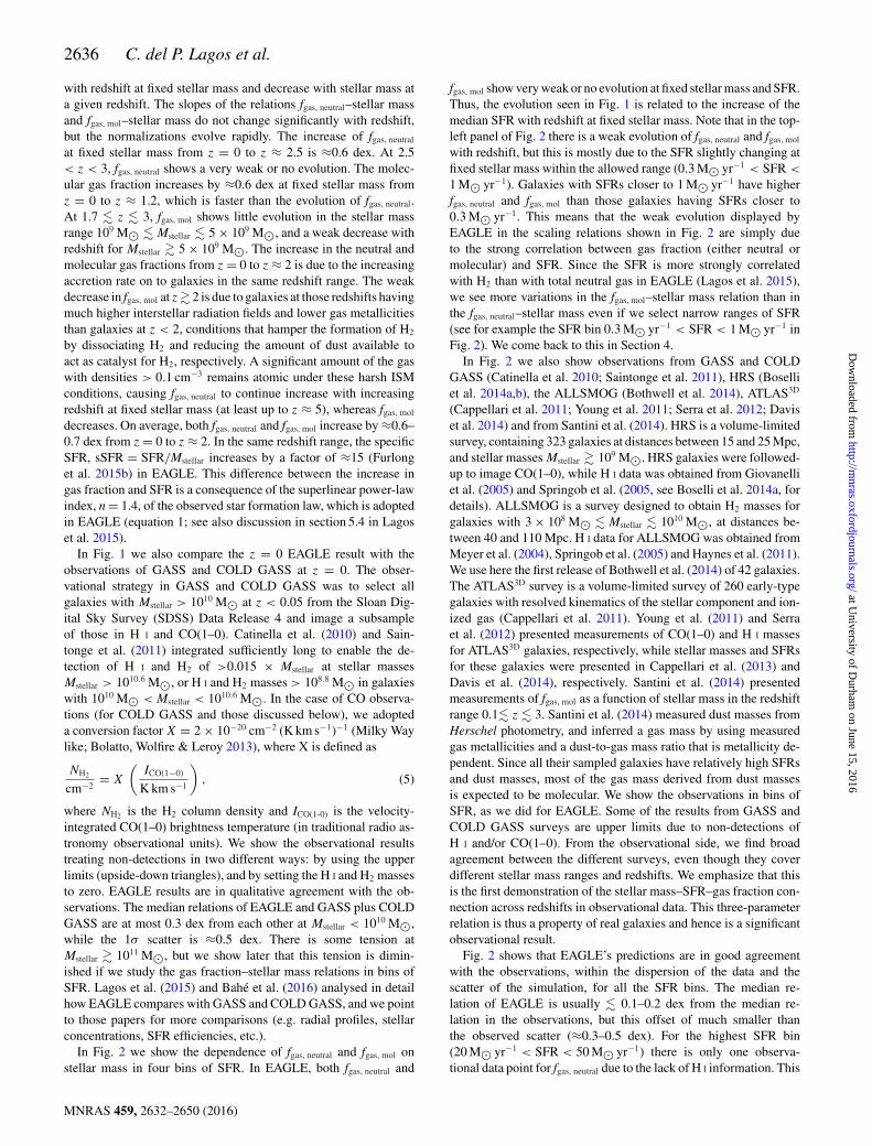
Figure 1. The neutral (equation 3; top panel) and molecular (equation 4;bottom panel) gas fractions as a function of stellar mass at z = 0, 0.5,1.2, 1.7, 2.5 and 3, as labelled, for the EAGLE simulation. Lines show themedian relations, and the hatched regions show the 16th–84th percentiles.For clarity, the latter are shown only for z = 0 and 1.7 galaxies. Solidlines show bins with >10 galaxies, while dotted lines show bins where thenumber of galaxies drops below 10. Observations at z = 0 from GASS andCOLD GASS are shown using two symbols: upside-down triangles show themedians if upper limits are taken for the non-detections, and triangles showthe median when we set H I and H2 masses to zero for the non-detections.The true median is bracketed by these two values. Error bars show the 1σ
scatter. EAGLE and the observations agree within 0.5 dex.
Here we show how these scaling relations evolve and compare withobservations. We define the neutral and molecular gas fractions as
fgas,neutral ≡ (MH I + MH2 )
(MH I + MH2 + Mstellar), (3)
fgas,mol ≡ (MH2 )
(MH2 + Mstellar). (4)
Note that we do not include the mass of ionized hydrogen in equa-tions (3) and (4) because it is hard to estimate observationally,which would make the task of comparing simulation with observa-tions difficult. Similarly, in equation (4) we do not include H I inthe denominator because for observations at z > 0 there is no H I
information.Fig. 1 shows fgas, neutral and fgas, mol as a function of stellar mass, for
all galaxies with Mstellar > 109 M� at redshifts 0 ≤ z ≤ 3 in EAGLE,to match the observed redshift range. Both gas fractions increase
MNRAS 459, 2632–2650 (2016)
at University of D
urham on June 15, 2016
http://mnras.oxfordjournals.org/
Dow
nloaded from
2636 C. del P. Lagos et al.
with redshift at fixed stellar mass and decrease with stellar mass ata given redshift. The slopes of the relations fgas, neutral–stellar massand fgas, mol–stellar mass do not change significantly with redshift,but the normalizations evolve rapidly. The increase of fgas, neutral
at fixed stellar mass from z = 0 to z ≈ 2.5 is ≈0.6 dex. At 2.5< z < 3, fgas, neutral shows a very weak or no evolution. The molec-ular gas fraction increases by ≈0.6 dex at fixed stellar mass fromz = 0 to z ≈ 1.2, which is faster than the evolution of fgas, neutral.At 1.7 � z � 3, fgas, mol shows little evolution in the stellar massrange 109 M� � Mstellar � 5 × 10⁹ M�, and a weak decrease withredshift for Mstellar � 5 × 10⁹ M�. The increase in the neutral andmolecular gas fractions from z = 0 to z ≈ 2 is due to the increasingaccretion rate on to galaxies in the same redshift range. The weakdecrease in fgas, mol at z� 2 is due to galaxies at those redshifts havingmuch higher interstellar radiation fields and lower gas metallicitiesthan galaxies at z < 2, conditions that hamper the formation of H2
by dissociating H2 and reducing the amount of dust available toact as catalyst for H2, respectively. A significant amount of the gaswith densities > 0.1 cm−3 remains atomic under these harsh ISMconditions, causing fgas, neutral to continue increase with increasingredshift at fixed stellar mass (at least up to z ≈ 5), whereas fgas, mol
decreases. On average, both fgas, neutral and fgas, mol increase by ≈0.6–0.7 dex from z = 0 to z ≈ 2. In the same redshift range, the specificSFR, sSFR = SFR/Mstellar increases by a factor of ≈15 (Furlonget al. 2015b) in EAGLE. This difference between the increase ingas fraction and SFR is a consequence of the superlinear power-lawindex, n = 1.4, of the observed star formation law, which is adoptedin EAGLE (equation 1; see also discussion in section 5.4 in Lagoset al. 2015).
In Fig. 1 we also compare the z = 0 EAGLE result with theobservations of GASS and COLD GASS at z = 0. The obser-vational strategy in GASS and COLD GASS was to select allgalaxies with Mstellar > 1010 M� at z < 0.05 from the Sloan Dig-ital Sky Survey (SDSS) Data Release 4 and image a subsampleof those in H I and CO(1–0). Catinella et al. (2010) and Sain-tonge et al. (2011) integrated sufficiently long to enable the de-tection of H I and H2 of >0.015 × Mstellar at stellar massesMstellar > 1010.6 M�, or H I and H2 masses > 108.8 M� in galaxieswith 1010 M� < Mstellar < 1010.6 M�. In the case of CO observa-tions (for COLD GASS and those discussed below), we adopteda conversion factor X = 2 × 10⁻²⁰ cm−2 (K km s−1)−1 (Milky Waylike; Bolatto, Wolfire & Leroy 2013), where X is defined as
NH2
cm−2= X
(ICO(1−0)
K km s−1
), (5)
where NH2 is the H2 column density and ICO(1-0) is the velocity-integrated CO(1–0) brightness temperature (in traditional radio as-tronomy observational units). We show the observational resultstreating non-detections in two different ways: by using the upperlimits (upside-down triangles), and by setting the H I and H2 massesto zero. EAGLE results are in qualitative agreement with the ob-servations. The median relations of EAGLE and GASS plus COLDGASS are at most 0.3 dex from each other at Mstellar < 1010 M�,while the 1σ scatter is ≈0.5 dex. There is some tension atMstellar � 1011 M�, but we show later that this tension is dimin-ished if we study the gas fraction–stellar mass relations in bins ofSFR. Lagos et al. (2015) and Bahe et al. (2016) analysed in detailhow EAGLE compares with GASS and COLD GASS, and we pointto those papers for more comparisons (e.g. radial profiles, stellarconcentrations, SFR efficiencies, etc.).
In Fig. 2 we show the dependence of fgas, neutral and fgas, mol onstellar mass in four bins of SFR. In EAGLE, both fgas, neutral and
fgas, mol show very weak or no evolution at fixed stellar mass and SFR.Thus, the evolution seen in Fig. 1 is related to the increase of themedian SFR with redshift at fixed stellar mass. Note that in the top-left panel of Fig. 2 there is a weak evolution of fgas, neutral and fgas, mol
with redshift, but this is mostly due to the SFR slightly changing atfixed stellar mass within the allowed range (0.3 M� yr−1 < SFR <
1 M� yr−1). Galaxies with SFRs closer to 1 M� yr−1 have higherfgas, neutral and fgas, mol than those galaxies having SFRs closer to0.3 M� yr−1. This means that the weak evolution displayed byEAGLE in the scaling relations shown in Fig. 2 are simply dueto the strong correlation between gas fraction (either neutral ormolecular) and SFR. Since the SFR is more strongly correlatedwith H2 than with total neutral gas in EAGLE (Lagos et al. 2015),we see more variations in the fgas, mol–stellar mass relation than inthe fgas, neutral–stellar mass even if we select narrow ranges of SFR(see for example the SFR bin 0.3 M� yr−1 < SFR < 1 M� yr−1 inFig. 2). We come back to this in Section 4.
In Fig. 2 we also show observations from GASS and COLDGASS (Catinella et al. 2010; Saintonge et al. 2011), HRS (Boselliet al. 2014a,b), the ALLSMOG (Bothwell et al. 2014), ATLAS3D
(Cappellari et al. 2011; Young et al. 2011; Serra et al. 2012; Daviset al. 2014) and from Santini et al. (2014). HRS is a volume-limitedsurvey, containing 323 galaxies at distances between 15 and 25 Mpc,and stellar masses Mstellar � 109 M�. HRS galaxies were followed-up to image CO(1–0), while H I data was obtained from Giovanelliet al. (2005) and Springob et al. (2005, see Boselli et al. 2014a, fordetails). ALLSMOG is a survey designed to obtain H2 masses forgalaxies with 3 × 10⁸ M� � Mstellar � 1010 M�, at distances be-tween 40 and 110 Mpc. H I data for ALLSMOG was obtained fromMeyer et al. (2004), Springob et al. (2005) and Haynes et al. (2011).We use here the first release of Bothwell et al. (2014) of 42 galaxies.The ATLAS3D survey is a volume-limited survey of 260 early-typegalaxies with resolved kinematics of the stellar component and ion-ized gas (Cappellari et al. 2011). Young et al. (2011) and Serraet al. (2012) presented measurements of CO(1–0) and H I massesfor ATLAS3D galaxies, respectively, while stellar masses and SFRsfor these galaxies were presented in Cappellari et al. (2013) andDavis et al. (2014), respectively. Santini et al. (2014) presentedmeasurements of fgas, mol as a function of stellar mass in the redshiftrange 0.1� z � 3. Santini et al. (2014) measured dust masses fromHerschel photometry, and inferred a gas mass by using measuredgas metallicities and a dust-to-gas mass ratio that is metallicity de-pendent. Since all their sampled galaxies have relatively high SFRsand dust masses, most of the gas mass derived from dust massesis expected to be molecular. We show the observations in bins ofSFR, as we did for EAGLE. Some of the results from GASS andCOLD GASS surveys are upper limits due to non-detections ofH I and/or CO(1–0). From the observational side, we find broadagreement between the different surveys, even though they coverdifferent stellar mass ranges and redshifts. We emphasize that thisis the first demonstration of the stellar mass–SFR–gas fraction con-nection across redshifts in observational data. This three-parameterrelation is thus a property of real galaxies and hence is a significantobservational result.
Fig. 2 shows that EAGLE’s predictions are in good agreementwith the observations, within the dispersion of the data and thescatter of the simulation, for all the SFR bins. The median re-lation of EAGLE is usually � 0.1–0.2 dex from the median re-lation in the observations, but this offset of much smaller thanthe observed scatter (≈0.3–0.5 dex). For the highest SFR bin(20 M� yr−1 < SFR < 50 M� yr−1) there is only one observa-tional data point for fgas, neutral due to the lack of H I information. This
MNRAS 459, 2632–2650 (2016)
at University of D
urham on June 15, 2016
http://mnras.oxfordjournals.org/
Dow
nloaded from

The fundamental plane of star formation 2637
Figure 2. The neutral (equation 3; top panels) and molecular (equation 4; bottom panels) gas fractions as a function of stellar mass in bins of SFR, as labelledin each panel. For EAGLE galaxies, lines show the medians, while the 16th–84th percentiles are shown as shaded regions (but only for z = 0 and 1.7 galaxies).We only show bins that have >10 galaxies. Symbols show the observational result of GASS and COLD GASS (Catinella et al. 2010 and Saintonge et al.2011; open circles), HRS (Boselli et al. 2014a; stars), ATLAS3D (Cappellari et al. 2011; Young et al. 2011; Serra et al. 2012; Davis et al. 2014; filled squares),ALLSMOG (Bothwell et al. 2014; filled circles) and Santini et al. (2014, open squares). Observations have been coloured according to their redshift followingthe same colour code we used for EAGLE galaxies (labelled in the right-hand panels). We see only weak evolution once the gas fraction–stellar mass relationis investigated in bins of SFR, with the remaining evolution being mostly due to evolution of the median SFR within each SFR bin. Overall, EAGLE agreeswell with the observations within 0.3 dex (with the scatter on the observations being of a similar magnitude).
MNRAS 459, 2632–2650 (2016)
at University of D
urham on June 15, 2016
http://mnras.oxfordjournals.org/
Dow
nloaded from

2638 C. del P. Lagos et al.
Table 2. Principal component analysis (PCA) of galaxies in the Ref-L100N1504 simulation. Galaxies with Mstellar > 109 M�, SFR > 0.01 M� yr−1,MH2 /(MH2 + Mstellar) > 0.01 and 0 ≤ z ≤ 4.5 were included in the analysis. The PCA was conducted with the variables: stellar mass, SFR, metallicityof the star-forming gas (ZSF, gas), molecular, atomic and neutral gas masses and the half-mass stellar radius r50, st. We adopt Z� = 0.0127. Beforeperforming the PCA, we renormalize all the components by subtracting the mean and dividing by the standard deviation (all in logarithm). In thetable we show the property each component relates to, but we remind the reader that we renormalize them before performing the PCA. The threefirst principal components account for 55 per cent, 24 per cent and 14 per cent, respectively, of the total variance, and therefore account together for93 per cent of the total variance. The first three PCA vectors are shown here.
(1) (2) (3) (4) (5) (6) (7)Comp. x1 x2 x3 x4 x5 x6 x7
Prop. log10
(MstellarM�
)log10
(SFR
M� yr−1
)log10
(ZSF,gas
Z�)
log10
(MH2M�
)log10
(MH I
M�)
log10
(Mneutral
M�)
log10
(r50,�
kpc
)
PC1 0.31 − 0.57 − 0.19 − 0.15 0.4 0.6 0.06PC2 0.46 0.04 − 0.31 − 0.51 0.22 − 0.61 0.09PC3 − 0.19 − 0.68 − 0.14 0.33 − 0.33 − 0.51 0.002
data point corresponds to the median of four galaxies belonging toGASS and COLD GASS. In the simulation there are no galaxieswith those SFRs at z = 0, which is due to its limited volume. GASSand COLD GASS are based on SDSS, which has a volume at z <
0.1 that is ≈10 times larger than the volume of the Ref-L100N1504simulation. Thus, the non-existence of such galaxies at z = 0 inEAGLE is not unexpected.
From Fig. 2 one concludes that there is a relation betweenfgas, neutral, stellar mass and SFR, and between fgas, mol, stellar massand SFR. These planes exist in both the simulation and the obser-vations, which is a significant result for EAGLE and observations.This motivates us to analyse more in detail how fundamental thesecorrelations are compared to the more widely-known scaling rela-tions introduced in Section 1. With this in mind we perform a PCAin the next section.
4 T H E F U N DA M E N TA L PL A N E O F S TA RF O R M AT I O N
4.1 A principal component analysis
With the aim of exploring which galaxy correlations are most funda-mental and how the gas fraction–SFR–stellar mass relations fit intothat picture, we perform a PCA over seven properties of galaxies inthe Ref-L100N1504 simulation. We do not include redshift in thelist of properties because we decide to only include properties ofgalaxies to make the interpretation of PCA more straightforward.However, we do analyse possible redshift trends in Section 4.2.We include all galaxies in EAGLE with Mstellar > 109 M�, SFR> 0.01 M� yr−1, Mneutral > 107 M� and at 0 ≤ z ≤ 4.5 in thePCA. Here Mneutral is the H I plus H2 mass. The PCA uses orthogo-nal transformations to find linear combinations of variables.
PCA is designed to return as the first principal component thecombination of variables that contains the largest possible varianceof the sample, with each subsequent component having the largestpossible variance under the constraint that it is orthogonal to theprevious components. In order to perform the PCA, we renormalizegalaxy properties in logarithmic space by subtracting the mean anddividing by the standard deviation of each galaxy property. Table 2shows the variables that were included in the PCA and shows thefirst three principal components. We apply equal weights to thegalaxies in the PCA, which is justified by the fact that the redshiftdistribution of galaxies with Mstellar > 109 M� is close to flat (seebottom panel of Fig. 5).
We find that the first principal component is dominated by thestellar mass, SFR and the neutral gas mass (and secondarily by
the atomic gas mass), with weaker dependences on the moleculargas mass and the gas metallicity. This component accounts for55 per cent of the variance of the galaxy population. The relationbetween the neutral gas fraction, SFR and stellar mass of galaxiesdefine a plane in the three-dimensional space, which we refer to as‘the Fundamental Plane of star formation’, that we explore in detailin Section 4.2. Since this plane accounts for most of the variance,it is one of the most fundamental relations of galaxies. This is animportant prediction of EAGLE.
The second principal component is dominated by the stellar mass,metallicity of the star-forming gas, and molecular and neutral gasmasses. This component is responsible for 24 per cent of the vari-ance of the galaxy population in EAGLE, and can be connectedwith the mass–metallicity relation and how its scatter is correlatedwith the molecular and neutral gas content. Note that molecular gasplays a secondary role compared to the neutral gas fraction. Thiswill be discussed in Section 4.3.
The third principal component shows a correlation between allthe gas components (molecular, atomic and neutral), SFR and sec-ondarily on stellar mass and gas metallicity. This principal compo-nent shows that galaxies tend to be simultaneously rich (or poor)in atomic and neutral (molecular plus atomic) hydrogen. Note thatthe half-mass radius does not strongly appear in the first three prin-cipal components. We find that r50, � appears in the fourth and fifthprincipal components, with dependences on the stellar mass andmolecular gas mass (no dependence of r50, � on gas metallicity isseen in our analysis).
We test how the PCA is affected by selecting subsamples ofgalaxies. Selecting galaxies with Mstellar > 1010 M� has the ef-fect of increasing the importance of the H2 mass and metallic-ity on the first principal component, while in the second prin-cipal component we see very little difference. However, we stillsee that the main properties defining the first principal compo-nent are the stellar mass, SFR and neutral gas mass. If instead,we select galaxies with Mstellar > 109 M� that are mostly passive(those with 0.001 M� yr−1 ≤ SFR ≤ 0.1 M� yr−1), we find thatthe first principal component changes very little, while in the secondprincipal component MH2 becomes as important as Mneutral. A se-lection of galaxies with Mstellar > 1010 M� and 0.001 M� yr−1 ≤SFR ≤ 0.1 M� yr−1 (which again correspond to mostly passivegalaxies), produces the PCA to give more weight to the gas metal-licity and the H2 mass in the first principal component, becomingmore dominated by the stellar mass, SFR, ZSF, gas and H2 and H I
masses. These tests show that the first principal component is al-ways related to the Fundamental Plane of star formation that weintroduce in Section 4.2 regardless of whether we select massive
MNRAS 459, 2632–2650 (2016)
at University of D
urham on June 15, 2016
http://mnras.oxfordjournals.org/
Dow
nloaded from

The fundamental plane of star formation 2639
galaxies only, passive galaxies or the entire galaxy population. Forgalaxies with SFRs � 0.1 M� yr−1, we see that the metallicity be-comes more prominent in the first principal component. The secondprincipal component in all the tests we did has the gas metallicityplaying an important role and therefore is always related to the MZrelation.
As an additional test to determine which gas phase is more impor-tant (neutral, atomic or molecular), we present in Appendix B threeprincipal component analyses, in which we include stellar mass,SFR, gas metallicity and H I, H2 or neutral gas mass. We find thatthe highest variance is obtained in the first principal component ofthe PCA that includes the neutral gas mass. If instead we includethe H I or H2 masses, we obtain a smaller variance on the first prin-cipal component. In addition, we find that the contribution of themetallicity of the star-forming gas in the first principal componentsof the PCA performed using the neutral or H I gas masses is negli-gible, while it only appears to be important if we use the H2 massinstead. This supports our interpretation that most of the variancein the galaxy population is enclosed in the ‘the Fundamental Planeof star formation’ of galaxies, and that the neutral gas mass is moreimportant than the H I or H2 masses alone. In the rest of this sectionwe analyse in detail the physical implications of the first two prin-cipal components presented in Table 2, which together account for79 per cent of the variance seen in the EAGLE galaxy population.
4.2 The Fundamental Plane of star formation
Here we investigate the dependence of the neutral and moleculargas fraction on stellar mass and SFR. We change from using gasmasses in Section 4.1 to gas fractions. The reason for this is thatthe scatter in the three-dimensional space of stellar mass, SFR andneutral gas fraction or molecular gas fraction is the least comparedto what it is obtained if we instead use gas masses or simply neutralor molecular gas mass to stellar mass ratios. We come back to thiswhen discussing equations (6) and (7).
In order to visualize a flat plane in a three-dimensional space,it helps to define vectors that are perpendicular and parallel to theplane, and plot them against each other in order to reveal edge-on andface-on orientations of the plane. This is what we do in this section.If we define a plane as ax + by + cz = 0, vector perpendiculars andparallel to the plane would be v⊥ = (a, b, c) and v‖ = (−b, −a, 0),respectively. We use these vectors later to show edge-on orientationsof the Fundamental Plane of star formation, which we introduce inequations (6) and (7).
Fig. 3 shows four views of the three-dimensional space of neutralgas fraction, stellar mass and SFR. In this figure we include allgalaxies in EAGLE with Mstellar > 109 M�, SFR ≥ 0.01 M� yr−1,and that are in the redshift range 0 ≤ z ≤ 4.5. We show the un-derlying redshift distribution of the galaxies by binning each planeand colouring bins according to the median redshift of the galaxies.Two of the views show edge-on orientations of the plane (i.e. withrespect to the best-fitting plane of equation 6 below), and the othertwo are projections along the axes of the three-dimensional space.One edge-on view (top-left panel) shows the neutral gas fraction as afunction of the combination of SFR and stellar mass of equation (6).For the second edge-on view (top-right panel), we use the perpen-dicular and parallel vectors defined above, with the plane beingdefined in equation (6).
Galaxies populate a well-defined plane, which shows little evo-lution. Galaxies evolve along this plane with redshift, in such a waythat they are on average more gas rich and more highly star-formingat higher redshift. When we consider the molecular gas fraction
instead of the neutral gas fraction, the situation is the same: galax-ies populate a well-defined plane in the three-dimensional space offgas, mol, stellar mass and SFR (shown in Fig. 4). This means that atfixed SFR and stellar mass, there is very little evolution in fgas, neutral
and fgas, mol. Hence, most of the observed trend of an increasingmolecular fraction with redshift (e.g. Geach et al. 2011; Saintongeet al. 2013) is related to the median SFR at fixed stellar mass in-creasing with redshift (e.g. Noeske et al. 2007; Sobral et al. 2014).We argue later that both the SFR and gas fraction are a consequenceof the self-regulation of star formation in galaxies.
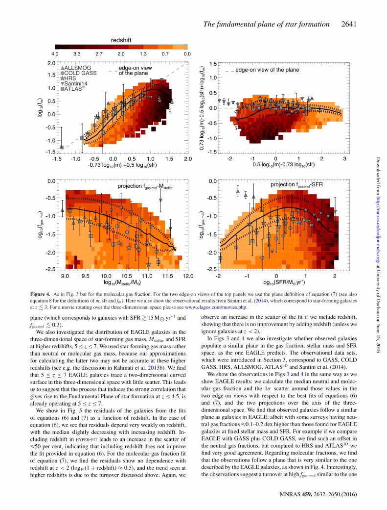
For both fgas, neutral and fgas, mol the relation is best described by acurved surface in three-dimensional space. Here we provide fits ofthe flat plane tangential to this two-dimensional surface at Mstellar =5 × 10¹⁰ M� and SFR = 2 M� yr−1, which we compute using theHYPER-FIT R package2 of Robotham & Obreschkow (2015). We referto the tangential plane fitted to the fgas,neutral–SFR–Mstellar relation as‘the Fundamental Plane of star formation’. For the fitting, we weigheach galaxy by the inverse of the number density in logarithmicmass interval in order to prevent the fit from being biased towardsthe more numerous small galaxies. The best-fitting planes are
0.85 log10(m) − 0.58 log10(sfr) + log10(fn) = 0, (6)
0.73 log10(m) − 0.50 log10(sfr) + log10(fm) = 0, (7)
where,
m = Mstellar
5 × 10¹⁰ M�, sfr = SFR
2 M� yr−1,
fn = fgas,neutral
0.046, fm = fgas,mol
0.026. (8)
The fits above are designed to minimize the scatter. The best fits ofequations (6) and (7) are shown as dashed lines in the top-left panelsof Figs 3 and 4, respectively. The standard deviations perpendicularto the planes calculated by HYPER-FIT are 0.17 dex for equation (6)and 0.15 dex for equation (7), while the standard deviations parallelto the gas fraction axis are 0.24 dex for equation (6) and 0.2 dex forequation (7). Although the scatter seen for the molecular gas fractionis slightly smaller than for the neutral gas fraction, the PCA points tothe latter as capturing most of the variance of the galaxy population.This is because the neutral gas fraction is more directly connectedto the process of gas accretion than the molecular gas fraction,and we discuss later that accretion is one of the key processesdetermining the existence of the fundamental planes. In addition,because SFR and the molecular gas mass are strongly correlated,only one of these properties is needed to describe most of thevariance among galaxy properties. We also analysed the correlationbetween fgas, neutral (fgas, mol) and sSFR, and found that the scatterincreases by ≈20 per cent (≈25 per cent) relative to the scattercharacterizing equation (6). We find that fitting planes to the three-dimensional dependency of gas mass–SFR–stellar mass or gas-to-stellar mass ratio–SFR–stellar mass (instead of gas fraction–SFR–stellar mass, as presented in equations 6 and 7) leads to an increasein the scatter relative to what is obtained around equations (6)and (7) of ≈20–30 per cent. We therefore conclude that the tightestcorrelations (i.e. least scatter) in EAGLE are those between gasfraction, stellar mass and SFR.
Note that there is a clear turnover at fgas, mol ≈ 0.3 (very clear ata y-axis value ≈0.7 in the top-left of Fig. 4), which is produced by
2 hyperfit.icrar.org/
MNRAS 459, 2632–2650 (2016)
at University of D
urham on June 15, 2016
http://mnras.oxfordjournals.org/
Dow
nloaded from

2640 C. del P. Lagos et al.
Figure 3. Four views of the distribution of galaxies in the three-dimensional space of neutral fraction, stellar mass and SFR. We include all EAGLE galaxieswith Mstellar > 109 M�, in the redshift range 0 ≤ z ≤ 4.5. The median and 16th and 84th percentiles are shown as solid and dotted lines, respectively, andare shown in all the panels. Filled squares are coloured according to the median redshift of galaxies in bins of the horizontal and vertical axis, as indicated inthe colour bar. The top panels show edge-on views of the fitted plane of equation (6), with the top-left panel showing normalized gas fraction as a function ofthe combination of SFR and stellar mass of equation (6) (see also equation 8 for the definitions of m, sfr and fn), while the top-right panel shows the vectorperpendicular to the plane, v⊥ = (a, b, c), as a function of a vector parallel to the plane, v‖ = (−b,−a, 0), where the plane is defined as ax + by + cz = 0(see equation 6). The bottom panels show two projections along the axes of the three-dimensional space that are nearly face-on views of the plane: fgas, neutral
versus stellar mass (left-hand panel) and fgas, neutral versus SFR (right-hand panel). The dashed lines in the top panels show edge-on views of the plane. Symbolsshow observations: squares correspond to GASS and COLD GASS, circles to HRS, squares to ATLAS3D, and triangles to the ALLSMOG survey, as labelledin the top-left panel. Observations follow a plane in the three-dimensional space of fgas, neutral, stellar mass and SFR that is very similar to the one predicted byEAGLE. For a movie rotating over the three-dimensional space please see www.clagos.com/movies.php.
galaxies with SFR � 15 M� yr−1. Most of the galaxies that producethis turnover are forming stars in an ISM with a very high medianpressure (SFR-weighted pressures of log10(〈P〉 k−1
B / cm−3 K) ≈6–7). The turnover is less pronounced in the neutral gas fractionrelation (top-left panel in Fig. 3). Most galaxies that lie around theturnover are at z � 2. The fact that we do not see such strongturnover in the neutral gas fraction is because galaxies with highSFRs have an intense radiation field that destroys H2 more effec-tively, moving the H I to H2 transition towards higher gas pressures.Thus, a significant fraction of the gas with densities nH � 1 cm−3
remains atomic at high-redshift. The effect of this on the H2 fractionis important, introducing the turnover at high H2 fractions seen inFig. 4.
For the neutral gas fraction we find that the fitted plane ofequation (6) is a good description of the neutral gas fractions of
galaxies in EAGLE (note that this is also true for the higher reso-lution simulations shown in Appendix A) at fgas, neutral � 0.5 (y-axisvalue ≈1 in the top-left of Fig. 3). However, at higher neutral gasfractions, the fit tends to overshoot the gas fraction by ≈0.1–0.2dex. The latter is not because the gas fraction saturates at ≈1, butbecause there is a physical change in the ratio of SFR to neutralgas mass from z = 0 towards high redshift, due to the superlinearstar formation law adopted in EAGLE and the ISM gas densityevolution. We come back to this point in Section 4.2.1. For themolecular gas fraction we find that the fit of equation (7) describesthe molecular gas fractions of EAGLE galaxies well in the regime0.02 � fgas,mol � 0.3 (−0.2 � log10(fm) � 1), while at lower and athigher fgas, mol the fit overshoots the true values of the gas fraction.At the high molecular gas fractions this is due to galaxies popu-lating the turnover discussed above, that deviates from the main
MNRAS 459, 2632–2650 (2016)
at University of D
urham on June 15, 2016
http://mnras.oxfordjournals.org/
Dow
nloaded from
The fundamental plane of star formation 2641
Figure 4. As in Fig. 3 but for the molecular gas fraction. For the two edge-on views of the top panels we use the plane definition of equation (7) (see alsoequation 8 for the definitions of m, sfr and fm). Here we also show the observational results from Santini et al. (2014), which correspond to star-forming galaxiesat z � 3. For a movie rotating over the three-dimensional space please see www.clagos.com/movies.php.
plane (which corresponds to galaxies with SFR � 15 M� yr−1 andfgas,mol � 0.3).
We also investigated the distribution of EAGLE galaxies in thethree-dimensional space of star-forming gas mass, Mstellar and SFRat higher redshifts, 5 ≤ z ≤ 7. We used star-forming gas mass ratherthan neutral or molecular gas mass, because our approximationsfor calculating the latter two may not be accurate at these higherredshifts (see e.g. the discussion in Rahmati et al. 2013b). We findthat 5 ≤ z ≤ 7 EAGLE galaxies trace a two-dimensional curvedsurface in this three-dimensional space with little scatter. This leadsus to suggest that the process that induces the strong correlation thatgives rise to the Fundamental Plane of star formation at z ≤ 4.5, isalready operating at 5 ≤ z ≤ 7.
We show in Fig. 5 the residuals of the galaxies from the fitsof equations (6) and (7) as a function of redshift. In the case ofequation (6), we see that residuals depend very weakly on redshift,with the median slightly decreasing with increasing redshift. In-cluding redshift in HYPER-FIT leads to an increase in the scatter of≈50 per cent, indicating that including redshift does not improvethe fit provided in equation (6). For the molecular gas fraction fitof equation (7), we find the residuals show no dependence withredshift at z < 2 (log10(1 + redshift) ≈ 0.5), and the trend seen athigher redshifts is due to the turnover discussed above. Again, we
observe an increase in the scatter of the fit if we include redshift,showing that there is no improvement by adding redshift (unless weignore galaxies at z < 2).
In Figs 3 and 4 we also investigate whether observed galaxiespopulate a similar plane in the gas fraction, stellar mass and SFRspace, as the one EAGLE predicts. The observational data sets,which were introduced in Section 3, correspond to GASS, COLDGASS, HRS, ALLSMOG, ATLAS3D and Santini et al. (2014).
We show the observations in Figs 3 and 4 in the same way as weshow EAGLE results: we calculate the median neutral and molec-ular gas fraction and the 1σ scatter around those values in thetwo edge-on views with respect to the best fits of equations (6)and (7), and the two projections over the axis of the three-dimensional space. We find that observed galaxies follow a similarplane as galaxies in EAGLE, albeit with some surveys having neu-tral gas fractions ≈0.1–0.2 dex higher than those found for EAGLEgalaxies at fixed stellar mass and SFR. For example if we compareEAGLE with GASS plus COLD GASS, we find such an offset inthe neutral gas fractions, but compared to HRS and ATLAS3D wefind very good agreement. Regarding molecular fractions, we findthat the observations follow a plane that is very similar to the onedescribed by the EAGLE galaxies, as shown in Fig. 4. Interestingly,the observations suggest a turnover at high fgas, mol similar to the one
MNRAS 459, 2632–2650 (2016)
at University of D
urham on June 15, 2016
http://mnras.oxfordjournals.org/
Dow
nloaded from

2642 C. del P. Lagos et al.
Figure 5. Top panel: residuals of simulated galaxies from equations (6)and (7) as a function of log10(1 + redshift). Here residuals are defined asax + by + cz, where a, b and c are defined in equations (6) and (7). Thesolid black line is the mean residual of galaxies with Mstellar > 109 M�from the fit of equation (6) to the Fundamental Plane, with the dashed linesindicating the 16th and 84th percentiles. The red long-dashed line and reddotted lines, are the corresponding median and percentiles residuals fromthe fit of equation (7). Note that the redshift at which the medians cross zerois set by the choice of normalization, and thus it has no physical meaning.Bottom panel: redshift distribution of the galaxies with Mstellar > 109 M�i,shown at the top panel.
displayed by EAGLE (see top-left panel of Fig. 4). This could pointto real galaxies forming stars in intense UV radiation fields, as wefind for EAGLE galaxies.
Overall, we find that the agreement with the observations is wellwithin the scatter of both the simulation and observations. Notethat galaxies in the observational sets used here were selected verydifferently and in some cases using complex criteria, which is easyto see in the nearly face-on views of the bottom panels of Figs 3 and4. For example, ATLAS3D and ALLSMOG differ by �1.5 dex inthe nearly face-on views. However, when the plane is seen edge-on,both observational data sets follow the same relations. This meansthat even though some samples are clearly very biased, like Santiniet al. (2014) towards gas-rich galaxies, when we place them in thethree-dimensional space of gas fraction, SFR and stellar mass, theylie on the same plane. The fact that observations follow a verysimilar plane in the three-dimensional space of gas fraction, SFRand stellar mass as EAGLE is remarkable.
4.2.1 Physical interpretation of the Fundamental Plane ofstar formation
We argue that the existence of the two-dimensional surfaces inthe three-dimensional space of stellar mass, SFR and neutral or
molecular gas fractions in EAGLE is due to the self-regulation ofstar formation in galaxies. The rate of star formation is controlledby the balance between gas cooling and accretion, which increasesthe gas content of galaxies, and stellar and BH-driven outflows, thatremove gas out of galaxies (see Booth & Schaye 2010, Schaye et al.2010, Lagos et al. 2011, Haas et al. 2013a for numerical experimentssupporting these views). In this picture, both the gas content and theSFR of galaxies change to reflect the balance between accretion andoutflows, and the ratio is determined by the assumed star formationlaw.
This interpretation is supported by the comparison of the refer-ence model we use here with model variations in EAGLE presentedin Appendix C. We show four models in which the efficiency ofAGN and stellar feedback is changed. We find that weakening thestellar feedback has the effect of changing the normalization of theplane, but most importantly, increasing the scatter around it, whilemaking feedback stronger tends to tighten the plane. The effectof AGN feedback is very mild due to most of the galaxies shownbeing on the main sequence of galaxies in the SFR–Mstellar plane,and therefore not affected by AGN feedback. A similar change inscatter is seen if we now look at models where the stellar feedbackstrength has a different scaling (i.e. depending on metallicity aloneor on the velocity dispersion of the dark matter). Both model vari-ations produce less feedback at higher redshift (z > 1; see fig. 5 inC15) compared to the reference model, which leads to both modelsproducing a more scattered ‘Fundamental Plane of star formation’at high redshift. If feedback was not sufficient to balance the gas in-flows, the scatter would increase even further, erasing the existenceof the Fundamental Plane of star formation discussed here.
We find that the curvature of the two-dimensional surface ismainly driven by how the gas populates the probability distributionfunction of densities in galaxies at different redshifts and how starformation depends on the density in EAGLE (see Section 2.1).Galaxies at high redshift tend to form stars at higher ISM pressuresthan galaxies at z = 0, on average (see fig. 12 in Lagos et al.2015), which together with the superlinear star formation law, leadto higher-redshift galaxies having higher star formation efficiencies(i.e. the ratio between the SFR and the gas content above the densitythreshold for star formation). In Appendix C we show that changingthe dependency of the SFR density on the gas density changes theslope of the plane significantly, supporting our interpretation.
4.2.2 Example galaxies residing in the Fundamental Plane of starformation
We select examples of galaxies of a similar stellar mass, SFR andneutral gas fraction at different redshifts to examine their similaritiesand differences. Fig. 6 shows the atomic and molecular columndensity maps and the optical gri images of four galaxies at z =0, 0.5, 1.0 and 2 with Mstellar ≈ 1.1 × 10¹⁰ M�, SFR ≈ 2 M� yr−1
and fgas, neutral ≈ 0.2. The optical images were created using radiativetransfer simulations performed with the code SKIRT (Baes et al. 2011)in the SDSS g, r and i filters (Doi et al. 2010). Dust extinctionwas implemented using the metal distribution of galaxies in thesimulation, and assuming 40 per cent of the metal mass is lockedup is dust grains (Dwek 1998). The images were produced usingparticles in spherical apertures of 30 pkpc around the centres ofsubhaloes (see Trayford et al. 2015, in preparation for more details).
At z = 0, SFR ≈ 2 M� yr−1 and fgas, neutral ≈ 0.2 are typicalvalues of galaxies with Mstellar ≈ 1010 M� in the main sequence ofstar formation. However, at higher redshifts, the normalization ofthe sequence increases, and therefore a galaxy with the stellar mass,
MNRAS 459, 2632–2650 (2016)
at University of D
urham on June 15, 2016
http://mnras.oxfordjournals.org/
Dow
nloaded from

The fundamental plane of star formation 2643
Figure 6. Visualization of four galaxies in EAGLE (at redshifts z = 0, 0.5, 1 and 2) which were chosen to have Mstellar ≈ 1010 M�, SFR ≈ 2 M� yr−1 andfgas, neutral ≈ 0.25. The redshift of each galaxy is shown in the H I and H2 maps. The H I and H2 maps are coloured by column density, according to the colourbars at the top, with column densities in units of cm−2. The right-hand panels show SDSS gri images, which were constructed using the radiative transfer codeSKIRT (Baes et al. 2011, see Trayford et al. in preparation for details). Particles are smoothed by 1 ckpc in the NH2 and NH I maps. H I and H2 maps have asize of 100 × 100 pkpc2, while the gri images are of 60 × 60 pkpc2 (scale that is shown in the middle panels as a white square frame). At the right of everyrow we show the integrated values for the stellar mass, SFR, neutral gas fraction, molecular gas fraction and the projected half-stellar mass radius. Masses andSFR were calculated in spherical apertures of 30 pkpc, while the radius is calculated using a 2D circular aperture of 30 pkpc (averaged over three orthogonalprojections).
SFR and neutral gas fraction above lies below the main sequence ofstar formation and is thus considered an unusually passive galaxy.None the less, it is illuminating to visually inspect galaxies of thesame properties at different redshifts.
We find that the z = 0 galaxy in Fig. 6 is an ordered disc (whichis a common feature of galaxies with these properties at z = 0),with most of the star formation proceeding in the inner parts of thegalaxy and in the disc (compare H2 mass with stellar density maps).
MNRAS 459, 2632–2650 (2016)
at University of D
urham on June 15, 2016
http://mnras.oxfordjournals.org/
Dow
nloaded from
2644 C. del P. Lagos et al.
However, in the z = 0.5 and 1 galaxies we see striking differences:the higher-redshift galaxies are smaller (see the values of their half-mass radius listed in Fig. 6), have more disturbed discs, have steeperH2 density profiles and are more clumpy. This is particularly evidentwhen we compare the z = 0 galaxy with its z = 1 counterpart withthe same integrated properties. The picture at z = 2 again changescompletely: the neutral gas of the z = 2 galaxy displays a veryirregular morphology with filaments at ≈50–100 pkpc from thegalaxy centre, which is much more evident in H I than in H2, butstill present in the latter. In the z = 2 galaxy, a significant fractionof the H2 is locked up in big clumps, which is in contrast with thesmooth distribution of H2 in the z = 0 galaxy.
Although galaxies follow a tight plane relating fgas, neutral, stellarmass and SFR with little redshift evolution, they can have strikinglydifferent morphologies even at fixed fgas, neutral, stellar mass andSFR. We analyse this in detail in an upcoming paper (Lagos et al.in preparation).
4.3 The mass–metallicity relation
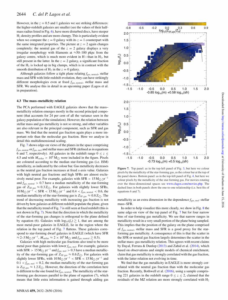
The PCA performed with EAGLE galaxies shows that the mass–metallicity relation emerges mostly in the second principal compo-nent (that accounts for 24 per cent of all the variance seen in thegalaxy population of the simulation). However, the relation betweenstellar mass and gas metallicity is not so strong, and other variablesare also relevant in the principal component, such as SFR and gasmass. We find that the neutral gas fraction again plays a more im-portant role than the molecular gas fraction. Here we analyse indetail this multidimensional scaling.
Fig. 7 shows edge-on views of the planes in the space comprisingfgas, neutral or fgas, mol and stellar mass and SFR (defined as in equations6 and 7, respectively). All galaxies in the redshift range 0 ≤ z ≤4.5 and with Mstellar > 109 M� were included in the figure. Pixelsare coloured according to the median star-forming gas (i.e. ISM)metallicity, as indicated by the colour bar. Gas metallicity decreasesas the neutral gas fraction increases at fixed x-axis value. Galaxieswith high neutral gas fractions and high SFRs are almost exclu-sively metal poor. For example, galaxies with SFR > 15 M� yr−1
and fgas, neutral > 0.7 have a median metallicity of the star-forminggas of ZSF,gas ≈ 0.3 Z�. For galaxies with slightly lower SFRs,10 M� yr−1 < SFR < 15 M� yr−1 and 0.4 < fgas, neutral < 0.6, themedian metallicity of the star-forming gas is ZSF,gas ≈ 0.8 Z�. Thetrend of decreasing metallicity with increasing gas fraction is notdriven by how galaxies at different redshift populate the plane, giventhat the metallicity trend of Fig. 7 is still seen at fixed redshift (this isnot shown in Fig. 7). Note that the direction in which the metallicityof the star-forming gas changes is orthogonal to the plane definedby equation (6). Galaxies with log10(fn) � 1, that are among themost metal-poor galaxies in EAGLE, lie in the region where therelation in the top panel of Fig. 7 flattens. These galaxies corre-spond to star-forming dwarf galaxies in EAGLE (which have SFR≈ 2–3 M� yr−1, Mstellar ≈ 2 × 10⁹ M� and fgas, neutral � 0.5).
Galaxies with high molecular gas fractions also tend to be moremetal poor than galaxies with lower fgas, mol. For example, galaxieswith SFR > 15 M� yr−1 and fgas, mol > 0.3 have a median metallic-ity of the star-forming gas of ZSF,gas ≈ 0.6 Z�. For galaxies withslightly lower SFRs, with 10 M� yr−1 < SFR < 15 M� yr−1 and0.1 < fgas, mol < 0.2, the median metallicity of the star-forming gasis ZSF,gas ≈ 1.2 Z�. However, the direction of the correlation hereis different to the one found for fgas, neutral. The metallicity of the star-forming gas decreases parallel to the plane of equation (7), whichmeans that little extra information is gained through adding gas
Figure 7. Top panel: as in the top-left panel of Fig. 3, but here we colourpixels by the metallicity of the star-forming gas, as the colour bar at the top ofthe panel shows. Bottom panel: as in the top-left panel of Fig. 4, but here wecolour pixels by the metallicity of the star-forming gas. For movies rotatingover the three-dimensional spaces see www.clagos.com/movies.php. Thedashed lines in both panels show the one-to-one relationship (i.e. best fits ofequations 6 and 7).
metallicity as an extra dimension in the dependence fgas, mol–stellarmass–SFR.
In order to help visualize this more clearly, we show in Fig. 8 thesame edge-on view of the top panel of Fig. 7 but for four narrowbins of star-forming gas metallicity. We see that narrow ranges inmetallicity result in a very small portion of the plane being sampled.This implies that the position of the galaxy on the plane comprisedof fgas, neutral, stellar mass and SFR is a good proxy for the star-forming gas metallicity. A consequence of this is that the scatter inthe SFR or neutral gas fraction largely determines the scatter in thestellar mass–gas metallicity relation. This agrees with recent claimsby Dayal, Ferrara & Dunlop (2013) and Zahid et al. (2014), whichbased on observations and simple models of chemical enrichment,claim that gas metallicity is strongly correlated with the gas fraction,with the latter relation not evolving in time.
We find that the gas metallicity in EAGLE is more strongly cor-related with the neutral gas fraction than with the molecular gasfraction. Recently, Bothwell et al. (2016), using a sample compris-ing 221 galaxies in the redshift range 0 ≤ z ≤ 2, claimed that theresiduals of the MZ relation are more strongly correlated with H2
MNRAS 459, 2632–2650 (2016)
at University of D
urham on June 15, 2016
http://mnras.oxfordjournals.org/
Dow
nloaded from

The fundamental plane of star formation 2645
Figure 8. As in the top panel of Fig. 7 but here we show four discrete binsin metallicity, as labelled. Galaxies in a narrow range of metallicity occupywell-defined regions of the Fundamental Plane of star formation.
than SFR. However, due to the lack of data, Bothwell et al. (2016)were not able to test whether atomic hydrogen or neutral hydrogenmasses are better predictions of the scatter than the H2 mass.
We use the HYPER-FIT R package of Robotham & Obreschkow(2015) to fit the dependence of ZSF, gas on stellar mass, SFR andfgas, neutral and find that the least scatter three-dimensional surfacehas a very weak dependence on stellar mass and SFR, and a strongdependence on fgas, neutral. This means that the metallicity of thestar-forming gas in galaxies can be predicted from the neutral gasfraction alone to within 40 per cent. We perform these fits inde-pendently of equations (6) and (7). The best fit between ZSF, gas andfgas, neutral is
log10
(ZSF,gas
Z�
)= −0.57 log10
(fgas,neutral
0.09
). (9)
The standard deviation perpendicular to the fitted relation ofequation (9) is 0.17 dex, while the standard deviation parallel tothe metallicity axis is 0.19 dex. We find that the metallicity canalso be predicted from a combination of the stellar mass and SFR,although with a slightly larger scatter:
log10
(ZSF,gas
Z�
)= 0.2 + 0.45 log10(m)
− 0.37 log10(sfr), (10)
where m and sfr are defined in equation (8). The standard deviationperpendicular to the fitted relation of equation (10) is 0.19 dex,while the scatter parallel to the metallicity axis is 0.2 dex. From thestandard deviations above, we can say that equations (9) and (10)are similarly good representations of ZSF, gas in EAGLE galaxies.
We assess the performance of the fits of equations (9) and (10)and compare with the observations of Mannucci et al. (2010) inFig. 9. In EAGLE, deviations from equations (10) and (9) are seenat ZSF, gas � 3 Z� and ZSF, gas � 0.7 Z�. However, 73 per cent of thegalaxies at 0 ≤ z ≤ 4.5 have 0.7 Z� ≤ ZSF, gas ≤ 3 Z�, and thus thefits of equations (9) and (10) are good descriptions of the majority ofthe galaxies in EAGLE. We also show how observed galaxies popu-late the plane of equation (10). For this we took the tabulated resultsfor the dependence of gas metallicity on SFR and stellar mass fromMannucci et al. (2010) and show here four bins of stellar mass. Wefind that observed galaxies follow a plane in the three-dimensionalspace of metallicity, SFR and stellar mass that is very similar to theone that EAGLE galaxies follow. The agreement between observa-
Figure 9. Top panel: edge-on view of the plane of equation (10), comprisedof star-forming gas metallicity, SFR and stellar mass in EAGLE. The thicksolid line and the dotted lines show the median and 1σ scatter, respectively,of all galaxies with Mstellar > 109 M� and SFR> 0.01 M� yr−1. We alsoshow the results for EAGLE galaxies in narrow bins of stellar masses in linesas labelled in the bottom panel. Observations at z = 0 from Mannucci et al.(2010) are shown for the same three bins of stellar mass we used for EAGLE.Observations are shown as symbols (labelled at the top-left corner). EAGLEgalaxies with Mstellar > 1010 M� and the observations agree to within 0.15dex, while lower-mass galaxies show discrepancies with the observations(up to ≈0.4 dex). To convert the observations of Mannucci et al. fromoxygen abundance to metallicity, we adopted a solar oxygen abundance of12 + log10(O/H)� = 8.69 and Z� = 0.0127. Bottom panel: as in the toppanel, but here we show an edge-on view of the relation between star-forminggas metallicity and neutral gas fraction (equation 9).
tions and EAGLE galaxies with Mstellar � 1010 M� is good (devia-tions are of �0.15 dex). However, galaxies with Mstellar < 1010 M�in the observations have metallicities that are ≈0.3–0.4 dex lowerthan EAGLE galaxies of the same stellar mass. This is consistentwith the discrepancies seen in the comparison presented in S15 be-tween the predicted MZ relation in EAGLE and the observations ofTremonti et al. (2004). S15 show that this is related to the resolutionof the simulation, as the higher resolution run that is recalibratedto reach a similar level of agreement with the z = 0.1 stellar massfunction and size–stellar mass relation, displays an MZ relation inmuch better agreement than the simulation we use here. The effectthis discrepancy has on the results presented in Fig. 9 is minimal be-cause the fit of equation (10) was calculated using the inverse of thenumber density as weight, and therefore low-mass galaxies, whichdisplay the largest discrepancies with the observed metallicity ofgalaxies, do not significantly skew the fit.
MNRAS 459, 2632–2650 (2016)
at University of D
urham on June 15, 2016
http://mnras.oxfordjournals.org/
Dow
nloaded from

2646 C. del P. Lagos et al.
5 C O N C L U S I O N S
We have studied the evolution of the gas fraction and the multidi-mensional dependence between stellar mass, SFR, gas fraction andgas metallicity in the EAGLE suite of hydrodynamical simulations.We use the gas phase transitions from ionized to neutral, and fromneutral to molecular, implemented on a particle-by-particle basesin post-processing by Lagos et al. (2015). The post-processing isdone using the fitting functions of Rahmati et al. (2013a) for thetransition from ionized to neutral gas, and of Gnedin & Kravtsov(2011) for the transition from neutral to molecular gas.
We summarize our main results below.
(i) We find that at fixed stellar mass, both the neutral and molec-ular gas fractions increase with redshift. In the case of the neutralgas fraction, this increase is a factor of ≈5 between z = 0 and ≈2.5,while the same increase is seen in the molecular gas fraction overa shorter time-scale, from z = 0 to z ≈ 1.5. The gas fractions athigher redshifts plateaus or even decreases. The sSFR on the otherhand increases by a factor of ≈15 over the same redshift interval.The difference is due to high-z galaxies having higher SFR/MH2
and SFR/Mneutral than z = 0 galaxies, which in turn is caused by thesuperlinear star formation law adopted in EAGLE and the highergas pressure at high redshift.
(ii) The evolution of the gas fraction is related to that of theSFR and the stellar mass. Galaxies show little evolution in their gasfraction at fixed stellar mass and SFR. This is a consequence ofgalaxies in EAGLE following with little scatter a two-dimensionalsurface in the three-dimensional space of stellar mass, SFR andneutral (or molecular) gas fraction. We term the plane tangentialto this surface at the mean location of galaxies the ‘FundamentalPlane of star formation’, and provide fits derived from EAGLE inequations (6) and (7). These two-dimensional surfaces are also seenin a compilation of observations of galaxies at 0 ≤ z ≤ 3 that wepresented here. Observed and simulated galaxies populate the three-dimensional space of SFR, stellar mass and gas fractions in a verysimilar manner. A PCA analysis reveals that the relation betweenthe neutral gas fraction, stellar mass and SFR contains most of thevariance (55 per cent) seen in the galaxy population of EAGLE,and therefore is one of the most fundamental correlations, whichwe term the ‘Fundamental Plane of star formation’.
(iii) We attribute the existence of the two-dimensional surfacesabove to the self-regulation of star formation in galaxies: SFR is setby the balance between the accretion and outflow of gas. We suggestthat the curvature of the plane in EAGLE is set by the model of starformation adopted, and affected by the relation between the ISMpressure and the SFR in EAGLE. We base these arguments onthe analysis of how the plane changes when we change the SNeand AGN feedback strength, the equation of state imposed on theunresolved ISM and the power-law index in the star formation lawadopted in EAGLE (Appendix C).
(iv) The positions of galaxies in the two-dimensional surfacein the space of gas fraction, SFR and stellar mass are very wellcorrelated with gas metallicity. The metallicity of the star-forminggas can therefore be predicted from the stellar masses and SFRsof galaxies, or from the neutral gas fraction of galaxies alone, towithin ≈40 per cent. This relation between metallicity, stellar mass,SFR and neutral gas fraction appears in the PCA in the secondcomponent, and contributes 24 per cent to the variance seen in thegalaxy population in EAGLE.
(v) The neutral gas fraction is more strongly correlated withthe scatter in the stellar mass–metallicity (MZ) relation than themolecular gas fraction. Upcoming surveys will be able to test these
predictions, as they will increase the number of galaxies sampledin their H I content by a factor of ≈100 (see for instance theaccepted proposals of the ASKAP H I All-Sky Survey,3 WAL-LABY, and the Deep Investigation of Neutral Gas Origins survey,4
DINGO; Johnston et al. 2008). Similarly, the Atacama Large Mil-limeter Array (ALMA5) and the NOrthern Extended MillimeterArray (NOEMA6) will be able to carry out a similar task but for H2
in galaxies.
This is the first time it has been shown in simulations and a largecompilation of observations that the stellar mass, SFR and gas frac-tion (either neutral or molecular) of galaxies follow a well-definedsurface in the three-dimensional space of stellar mass, SFR and neu-tral (or molecular) gas fraction. The fidelity to which EAGLE pre-dictions describe the observations is remarkable, particularly sincewe focused on galaxy properties that were not used to constrain anyof the free parameters in the subgrid models.
AC K N OW L E D G E M E N T S
We thank Luca Cortese, Matt Bothwell, Paola Santini and TimDavis for providing observational data sets, and Aaron Robotham,Luca Cortese and Barbara Catinella for useful discussions.CdPL is funded by a Discovery Early Career Researcher Award(DE150100618). CdPL also thanks the MERAC Foundation for aPostdoctoral Research Award. This work used the DiRAC DataCentric system at Durham University, operated by the Institutefor Computational Cosmology on behalf of the STFC DiRACHPC Facility (www.dirac.ac.uk). This equipment was funded byBIS National E-infrastructure capital grant ST/K00042X/1, STFCcapital grant ST/H008519/1, and STFC DiRAC Operations grantST/K003267/1 and Durham University. DiRAC is part of the Na-tional E-Infrastructure. Support was also received via the Interuni-versity Attraction Poles Programme initiated by the Belgian SciencePolicy Office ([AP P7/08 CHARM]), the National Science Foun-dation under grant no. NSF PHY11-25915, and the UK Scienceand Technology Facilities Council (grant numbers ST/F001166/1and ST/I000976/1) via rolling and consolidating grants awardedto the ICC. The research was supported in part by the EuropeanResearch Council under the European Union‘s Seventh Frame-work Programme (FP7/2007-2013)/ERC grant agreement 278594-GasAroundGalaxies.
R E F E R E N C E S
Baes M., Verstappen J., De Looze I., Fritz J., Saftly W., Vidal Perez E.,Stalevski M., Valcke S., 2011, ApJS, 196, 22
Bahe Y. M. et al., 2016, MNRAS, 456, 1115Benson A. J., Bower R., 2010, MNRAS, 405, 1573Bolatto A. D., Wolfire M., Leroy A. K., 2013, ARA&A, 51, 207Booth C. M., Schaye J., 2010, MNRAS, 405, L1Boselli A., Cortese L., Boquien M., 2014a, A&A, 564, A65Boselli A., Cortese L., Boquien M., Boissier S., Catinella B., Lagos C.,
Saintonge A., 2014b, A&A, 564, A66Bothwell M. S., Maiolino R., Kennicutt R., Cresci G., Mannucci F., Marconi
A., Cicone C., 2013, MNRAS, 433, 1425Bothwell M. S. et al., 2014, MNRAS, 445, 2599Bothwell M. S., Maiolino R., Peng Y., Cicone C., Griffith H., Wagg J., 2016,
MNRAS, 455, 1156
3 http://www.atnf.csiro.au/research/WALLABY/proposal.html4 http://askap.org/dingo5 http://almaobservatory.org/6 http://iram-institute.org/EN/noema-project.php
MNRAS 459, 2632–2650 (2016)
at University of D
urham on June 15, 2016
http://mnras.oxfordjournals.org/
Dow
nloaded from

The fundamental plane of star formation 2647
Brinchmann J., Charlot S., White S. D. M., Tremonti C., Kauffmann G.,Heckman T., Brinkmann J., 2004, MNRAS, 351, 1151
Brown T., Catinella B., Cortese L., Kilborn V., Haynes M. P., Giovanelli R.,2015, MNRAS, 452, 2479
Cappellari M. et al., 2011, MNRAS, 413, 813Cappellari M. et al., 2013, MNRAS, 432, 1862Catinella B. et al., 2010, MNRAS, 403, 683Chabrier G., 2003, PASP, 115, 763Crain R. A. et al., 2015, MNRAS, 450, 1937 (C15)Daddi E. et al., 2007, ApJ, 670, 156Dalla Vecchia C., Schaye J., 2012, MNRAS, 426, 140Damen M., Labbe I., Franx M., van Dokkum P. G., Taylor E. N., Gawiser
E. J., 2009, ApJ, 690, 937Dave R., Finlator K., Oppenheimer B. D., 2012, MNRAS, 421, 98Davis T. A. et al., 2014, MNRAS, 444, 3427Dayal P., Ferrara A., Dunlop J., 2013, MNRAS, 430, 2891De Rossi M. E., Theuns T., Font A. S., McCarthy I. G., 2015, MNRAS, 452,
486Dessauges-Zavadsky M. et al., 2015, A&A, 577, A50Doi M. et al., 2010, AJ, 139, 1628Dolag K., Borgani S., Murante G., Springel V., 2009, MNRAS, 399, 497Dwek E., 1998, ApJ, 501, 643Furlong M. et al., 2015a, preprint (arXiv:1510.05645)Furlong M. et al., 2015b, MNRAS, 450, 4486Geach J. E., Smail I., Moran S. M., MacArthur L. A., Lagos C. d. P., Edge
A. C., 2011, ApJ, 730, L19Giovanelli R. et al., 2005, AJ, 130, 2598Gnedin N. Y., Draine B. T., 2014, ApJ, 795, 37Gnedin N. Y., Kravtsov A. V., 2011, ApJ, 728, 88Haardt F., Madau P., 2001, in Neumann D. M., Tran J. T. T., eds, XXIst
Moriond Astrophysics Meeting, Recent results of XMM-Newton andChandra, Clusters of Galaxies and the High Redshift Universe Observedin X-rays, CEA, Saclay, p. 64
Haas M. R., Schaye J., Booth C. M., Dalla Vecchia C., Springel V., TheunsT., Wiersma R. P. C., 2013a, MNRAS, 435, 2931
Haas M. R., Schaye J., Booth C. M., Dalla Vecchia C., Springel V., TheunsT., Wiersma R. P. C., 2013b, MNRAS, 435, 2955
Haynes M. P. et al., 2011, AJ, 142, 170Herrera-Camus R. et al., 2012, ApJ, 752, 112Hughes T. M., Cortese L., Boselli A., Gavazzi G., Davies J. I., 2013, A&A,
550, A115Johnston S. et al., 2008, Exp. Astron., 22, 151Kennicutt R. C., Jr, 1998, ApJ, 498, 541Krumholz M. R., 2013, MNRAS, 436, 2747Lagos C. D. P., Lacey C. G., Baugh C. M., Bower R. G., Benson A. J., 2011,
MNRAS, 416, 1566Lagos C. d. P. et al., 2015, MNRAS, 452, 3815Lara-Lopez M. A. et al., 2010, A&A, 521, L53Lara-Lopez M. A. et al., 2013, MNRAS, 433, L35McAlpine S. et al., 2015, Astron. Comput., 15, 72Mannucci F., Cresci G., Maiolino R., Marconi A., Gnerucci A., 2010,
MNRAS, 408, 2115Marigo P., 2001, A&A, 370, 194Meyer M. J. et al., 2004, MNRAS, 350, 1195Noeske K. G. et al., 2007, ApJ, 660, L43Pawlik A. H., Schaye J., 2008, MNRAS, 389, 651Planck Collaboration XVI, 2014, A&A, 571, A16Portinari L., Chiosi C., Bressan A., 1998, A&A, 334, 505Rahmati A., Pawlik A. H., Raicevic M., Schaye J., 2013a, MNRAS, 430,
2427Rahmati A., Schaye J., Pawlik A. H., Raicevic M., 2013b, MNRAS, 431,
2261Richings A. J., Schaye J., Oppenheimer B. D., 2014, MNRAS, 442, 2780Robotham A. S. G., Obreschkow D., 2015, PASA, 32, e033Rodighiero G. et al., 2010, A&A, 518, L25Rosas-Guevara Y. M. et al., 2015, MNRAS, 454, 1038Saintonge A. et al., 2011, MNRAS, 415, 32Saintonge A. et al., 2013, ApJ, 778, 2
Salim S., Lee J. C., Ly C., Brinchmann J., Dave R., Dickinson M., SalzerJ. J., Charlot S., 2014, ApJ, 797, 126
Salim S., Lee J. C., Dave R., Dickinson M., 2015, ApJ, 808, 25Santini P. et al., 2009, A&A, 504, 751Santini P. et al., 2014, A&A, 562, A30Schaller M., Dalla Vecchia C., Schaye J., Bower R. G., Theuns T., Crain
R. A., Furlong M., McCarthy I. G., 2015, MNRAS, 454, 2277Schaye J., 2001, ApJ, 562, L95Schaye J., 2004, ApJ, 609, 667Schaye J., Dalla Vecchia C., 2008, MNRAS, 383, 1210Schaye J. et al., 2010, MNRAS, 402, 1536Schaye J. et al., 2015, MNRAS, 446, 521 (S15)Serra P. et al., 2012, MNRAS, 2823Sobral D., Best P. N., Smail I., Mobasher B., Stott J., Nisbet D., 2014,
MNRAS, 437, 3516Somerville R. S., Dave R., 2015, ARA&A, 53, 51Springel V., 2005, MNRAS, 364, 1105Springel V., White S. D. M., Tormen G., Kauffmann G., 2001, MNRAS,
328, 726Springel V. et al., 2008, MNRAS, 391, 1685Springob C. M., Haynes M. P., Giovanelli R., Kent B. R., 2005, ApJS, 160,
149Tacconi L. J. et al., 2013, ApJ, 768, 74Thielemann F.-K. et al., 2003, in Hillebrandt W., Leibundgut B., eds, From
Twilight to Highlight: The Physics of Supernovae. Springer-Verlag,Berlin, p. 331
Trayford J. W. et al., 2015, MNRAS, 452, 2879Tremonti C. A. et al., 2004, ApJ, 613, 898Wiersma R. P. C., Schaye J., Smith B. D., 2009a, MNRAS, 393, 99Wiersma R. P. C., Schaye J., Theuns T., Dalla Vecchia C., Tornatore L.,
2009b, MNRAS, 399, 574Young L. M. et al., 2011, MNRAS, 414, 940Zahid H. J., Dima G. I., Kudritzki R.-P., Kewley L. J., Geller M. J., Hwang
H. S., Silverman J. D., Kashino D., 2014, ApJ, 791, 130
A P P E N D I X A : ST RO N G A N D W E A KC O N V E R G E N C E T E S T S
S15 introduced the concept of ‘strong’ and ‘weak’ convergencetests. Strong convergence refers to the case where a simulation isrerun with higher resolution (i.e. better mass and spatial resolution)adopting exactly the same subgrid physics and parameters. Weakconvergence refers to the case when a simulation is rerun with higherresolution but the subgrid parameters are recalibrated to recover,as far as possible, similar agreement with the adopted calibrationdiagnostic (in the case of EAGLE, the z = 0.1 galaxy stellar massfunction and disc sizes of galaxies).
S15 introduced two higher-resolution versions of EAGLE, bothin a box of (25 cMpc)3 and with 2 × 7523 particles, Ref-L025N0752and Recal-L025N0752 (Table A1 shows some details of these sim-ulations). These simulations have better spatial and mass resolutionthan the intermediate-resolution simulations by factors of 2 and 8,respectively. In the case of Ref-L025N0752, the parameters of thesubgrid physics are kept fixed (and therefore comparing with thissimulation is a strong convergence test), while the simulation Recal-L025N0752 has four parameters whose values have been slightlymodified with respect to the reference simulation (and thereforecomparing with this simulation is a weak convergence test).
Here we compare the results presented throughout the paperobtained using the Ref-L100N1504 simulation with the resultsof the higher-resolution simulations Ref-L025N0752 and Recal-L025N0752.
Fig. A1 shows the neutral gas fraction as a function of the neutralgas fraction calculated from the stellar masses and SFRs of galaxies(i.e. applying equation 6). We show the relation for the simulations
MNRAS 459, 2632–2650 (2016)
at University of D
urham on June 15, 2016
http://mnras.oxfordjournals.org/
Dow
nloaded from

2648 C. del P. Lagos et al.
Table A1. EAGLE simulations used in this appendix. The columns list: (1) the name of the simulation, (2) comoving box size, (3) number of particles,(4) initial particle masses of gas and (5) dark matter, (6) comoving gravitational softening length, and (7) maximum proper comoving Plummer-equivalent gravitational softening length. Units are indicated below the name of column. EAGLE adopts (6) as the softening length at z ≥ 2.8, and (7)at z < 2.8. The simulation Recal-L025N0752 has the same masses of particles and softening length values than the simulation Ref-L025N0752.
(1) (2) (3) (4) (5) (6) (7)Name L No. of particles Gas particle mass DM particle mass Softening length Max. gravitational softeningUnits (cMpc) (M�) (M�) (ckpc) (pkpc)
Ref-L025N0376 25 2 × 3763 1.81 × 10⁶ 9.7 × 10⁶ 2.66 0.7Ref-L025N0752 25 2 × 7523 2.26 × 10⁵ 1.21 × 10⁶ 1.33 0.35
Figure A1. Strong and weak convergence tests. Top panel: the neutral gasfraction of galaxies, defined as in equation (3), in the simulations Ref-L025N0376, Ref-L025N0752 and Recal-L025N0752 at z = 0, as a functionof the neutral gas fraction calculated from the stellar masses and SFRs ofgalaxies by applying equation (6). We include all galaxies with Mstellar >
109 M�. Lines with error bars show the medians and the 16th and 84thpercentiles, respectively. The dotted line shows the relation fgas, neutral ≡fneutral, fit. Bottom panel: as in the top panel but at z = 1.2.
Ref-L025N0376, Ref-L025N0752 and Recal-L025N0752 at z = 0and 1.2. We find that Ref-L025N0376 follows the same relationas Ref-L100N1504, showing that the box size has no effect on theresults. The higher-resolution runs are very similar, both in terms ofthe median and the scatter of the relation. Deviations of the high-resolution runs from the Ref-L025N0376 simulation are of �0.2dex at z = 0 and of �0.1 dex at z = 1.2, with the largest valuescorresponding to galaxies with fgas, neutral �0.25.
In the case of the molecular gas fraction (Fig. A2), we find thatdeviations of the high-resolution runs from the Ref-L025N0376simulations are � 0.1 dex at z = 0 and � 0.25 dex at z = 1.2. Thescatter of the relations does not vary with resolution. Galaxies show-ing the largest variations with resolution are those that have fgas, mol
� 0.1 at z � 1 that populate the turnover of the relation betweenmolecular fraction, stellar mass and SFR. Interestingly, we find thatRecal-L025N0752 deviates more from Ref-L025N0376 than Ref-
Figure A2. As in Fig. A1 but for the molecular gas fraction, defined as inequation (4). We use equation (7) to calculate the molecular gas fractionfrom the stellar masses and SFRs of galaxies.
L025N0752 in the metrics used here. This is due to gas metallicitiesin Recal-L025N0752 being on average a factor of ≈2 lower thanthe gas metallicities in Ref-L025N0376 and Ref-L025N0752 (seeS15 for details). This influences the density threshold for star for-mation and explicitly enters in the second principal component ofSection 4.1.
We conclude that there is good convergence of the results for thegas fractions with the numerical resolution.
A P P E N D I X B : PR I N C I PA L C O M P O N E N TA NA LY S I S
Here we perform three principal component analyses over stellarmass, SFR, metallicity of the star-forming gas and H I, H2 or totalneutral gas mass. We do this with the aim of studying how muchthe variance contained in the first and second principal componentschange if only one gas phase mass is included. If the ‘FundamentalPlane of star formation of galaxies’ is indeed responsible for mostof the variance seen in the galaxy population, we should find stellarmass, SFR and neutral gas mass in the first principal component,
MNRAS 459, 2632–2650 (2016)
at University of D
urham on June 15, 2016
http://mnras.oxfordjournals.org/
Dow
nloaded from

The fundamental plane of star formation 2649
Table B1. PCA of galaxies in the Ref-L100N1504 simulation. Galaxies with Mstellar > 109 M�, SFR < 0.01 M� yr−1 and MH2 /(MH2 + Mstellar) >
0.01 and in the redshift range 0 ≤ z ≤ 4.5 were included in the analysis. The PCA was conducted with the variables stellar mass, SFR, metallicity ofthe star-forming gas and H I, H2 or total neutral gas mass. Here we show the first two principal components for each PCA together with the variancethey are responsible for.
(1) (2) (3) (4) (5) (6)Vector x1 x2 x3 x4
Property Variance MstellarM�
SFRM� yr−1
ZSF,gasZ�
MH2M�
PC1 59 per cent 0.49 0.5 0.58 0.4PC2 35 per cent 0.59 −0.24 0.21 −0.74
Property MstellarM�
SFRM� yr−1
ZSF,gasZ�
MH I
M�PC1 58 per cent 0.28 0.76 0.06 −0.59PC2 34 per cent 0.6 0.18 −0.63 0.45
Property MstellarM�
SFRM� yr−1
ZSF,gasZ�
MneutralM�
PC1 61 per cent 0.36 0.69 0.05 −0.62PC2 34 per cent 0.62 0.03 −0.71 0.34
and being responsible for the largest variance compared to principalcomponent vectors we obtain if we were to use atomic or moleculargas masses instead.
The three PCA are shown in Table B1. In the first PCA (whichuses MH2 ), the first principal component (PC1) has a strong contri-bution from the gas metallicity, which we do not see in PC1 whenMH I or Mneutral are used instead of MH2 . We see that PC1 in the caseMneutral is used has the largest variance, which is what we expectedif the Fundamental Plane of star formation introduced in Section 4.2was indeed responsible for most of the variance seen in the galaxypopulation. This confirms the analysis presented in Section 4. Weagain see that the metallicity of the star-forming gas has a largeweight in the second principal component in the three case weanalyse here.
APPENDIX C : EFFECTS O F SUBGRIDM O D E L L I N G O N T H E FU N DA M E N TA L PL A N EO F S TA R F O R M AT I O N
One of the main advantages of the EAGLE hydrodynamical simu-lation suite is that it includes a series of runs in which the subgridmodels and model parameters are varied, in addition to the refer-ence run that we analysed in Sections 3 and 4. C15 introduced nineruns in which the parameters of the reference model are altered (seetable 1 in C15). Here we show how the Fundamental Plane of starformation in EAGLE is affected by changes in the stellar and AGNfeedback strength and model, in the polytropic index of the equationof state applied to gas particles that have temperatures below an im-posed temperature floor, and in the power-law index adopted in thestar formation law (see Section 2.1 for details). We use the modelsof Table C1 to study how the relation between neutral gas fraction,SFR and stellar mass changes under changes in the parameters ofthe subgrid physics.
We find that changing the strength of stellar feedback (WeakFBand StrongFB; top panel in Fig. C1) has a mild effect on the nor-malization of the Fundamental Plane of star formation. Weakerfeedback produces higher neutral gas fractions at fixed stellar massand SFR with respect to the reference model (and the opposite istrue for stronger feedback). Under self-regulation of star formation,weaker feedback would produce lower outflow rates, which in turnproduces higher gas fraction and SFRs compared to stronger feed-back. Note that the median relations in the models with weak/strongstellar feedback are almost parallel to each other which supports our
Table C1. Variations of the reference model studied here. These variationswere run in the L025N0376 set-up (a simulation in a cubic volume oflength 25 cMpc on a side, using 3763 particles of dark matter and an equalnumber of baryonic particles; see Table A1 for more details). The referencemodel has the following parameter values: fth, max = 3.0, fth, min = 0.3(govern the stellar feedback strength), log10(�TAGN/K) = 8.5 (governs theAGN feedback strength), γ eos = 4/3 (governs the relation between pressureand density for gas particles with temperatures below Teos = 8 × 10³ K),and a power-law dependence in the star formation law of n = 1.4. In thebottom two models, the scaling of fth is changed to depend on the velocitydispersion of the DM (FBσ ) and on the gas metallicity alone (FBZ). In thereference model, fth depends on gas metallicity and density. See Section 2.1for a description of the subgrid models and more details on the parametersincluded in EAGLE.
(1) (2)Model Parameters changed
WeakFB fth,max = 1.5, fth,min = 0.15StrongFB fth, max = 6, fth, min = 0.6AGNTd8 log10(�TAGN/K) = 8AGNTd9 log10(�TAGN/K) = 9eos1 γ eos = 1eos5/3 γ eos = 5/3KSNormHi n = 4.8KSNormLow n = 0.48Model fth-scalingFBσ σ 2
DMFBZ ZSF, gas
interpretation that the curvature of the Fundamental Plane of starformation is set by the physics of star formation (i.e. how the gasgets converted into stars), while the normalization is set by theself-regulation of star formation. The effect of the self-regulationis suggested by the change in the scatter of the Fundamental Planewhen different feedback strengths are adopted. A weaker feed-back produces larger scatter, consistent with the less efficient self-regulation. A change in the scatter is also seen if we change themodel of stellar feedback (FBZ and FBσ models), where both leadto an increase in the scatter, due to the change in the time-scaleof self-regulation. Regarding the curvature, we see that changingthe index in the equation of state imposed on the unresolved ISM,γ eos (next-to-bottom panel in Fig. C1), does not change the nor-malization of the Fundamental Plane of star formation, but changesthe slope. For example, model eos5/3 produces a slightly steeper
MNRAS 459, 2632–2650 (2016)
at University of D
urham on June 15, 2016
http://mnras.oxfordjournals.org/
Dow
nloaded from
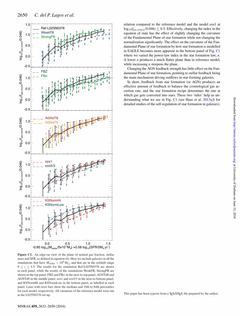
2650 C. del P. Lagos et al.
Figure C1. An edge-on view of the plane of neutral gas fraction, stellarmass and SFR, as defined in equation (6). Here we include galaxies in all thesimulations that have Mstellar > 109 M� and that are in the redshift range0 ≤ z ≤ 4.5. The results for the simulation Ref-L025N0376 are shownin each panel, while the results of the simulations WeakFB, StrongFB areshown in the top panel, FBZ and FBσ in the next-to-top panel, AGNTd8 andAGNTd9 in the middle panel, eos1 and eos5/3 in the next-to-bottom panel,and KSNormHi and KSNormLow in the bottom panel, as labelled in eachpanel. Lines with error bars show the medians and 16th to 84th percentilesfor each model, respectively. All variations of the reference model were runin the L025N0376 set-up.
relation compared to the reference model and the model eos1 atlog10(fgas,neutral/0.046) � 0.5. Effectively, changing the index in theequation of state has the effect of slightly changing the curvatureof the Fundamental Plane of star formation while not changing thenormalization significantly. The effect on the curvature of the Fun-damental Plane of star formation by how star formation is modelledin EAGLE becomes more apparent in the bottom panel of Fig. C1where we varied the power-law index in the star formation law, n.A lower n produces a much flatter plane than in reference model,while increasing n steepens the plane.
Changing the AGN feedback strength has little effect on the Fun-damental Plane of star formation, pointing to stellar feedback beingthe main mechanism driving outflows in star-forming galaxies.
In short, feedback from star formation (or AGN) produces aneffective amount of feedback to balance the cosmological gas ac-cretion rate, and the star formation recipe determines the rate atwhich gas gets converted into stars. These two ‘rules’ help us un-derstanding what we see in Fig. C1 (see Haas et al. 2013a,b fordetailed studies of the self-regulation of star formation in galaxies).
This paper has been typeset from a TEX/LATEX file prepared by the author.
MNRAS 459, 2632–2650 (2016)
at University of D
urham on June 15, 2016
http://mnras.oxfordjournals.org/
Dow
nloaded from

![arXiv:1606.02009v2 [cs.CV] 23 May 2017Salman Khan1; 2, Xuming He3y, Fatih Porikli , Mohammed Bennamoun4 Ferdous Sohel5 and Roberto Togneri4 1Data61-CSIRO, Canberra, Australia 2Australian](https://img.dokumen.tips/doc/110x75/5f8c8f959b6d0833d7742158/arxiv160602009v2-cscv-23-may-2017-salman-khan1-2-xuming-he3y-fatih-porikli.jpg)