Embed Size (px)
Citation preview

Durham E-Theses
Dissecting the theories of lanthanide magnetic
resonance
FUNK, ALEXANDER,MAX
How to cite:
FUNK, ALEXANDER,MAX (2014) Dissecting the theories of lanthanide magnetic resonance, Durhamtheses, Durham University. Available at Durham E-Theses Online: http://etheses.dur.ac.uk/10905/
Use policy
The full-text may be used and/or reproduced, and given to third parties in any format or medium, without prior permission orcharge, for personal research or study, educational, or not-for-pro�t purposes provided that:
• a full bibliographic reference is made to the original source
• a link is made to the metadata record in Durham E-Theses
• the full-text is not changed in any way
The full-text must not be sold in any format or medium without the formal permission of the copyright holders.
Please consult the full Durham E-Theses policy for further details.
Academic Support O�ce, Durham University, University O�ce, Old Elvet, Durham DH1 3HPe-mail: [email protected] Tel: +44 0191 334 6107
http://etheses.dur.ac.uk

Dissecting the theories of lanthanide
magnetic resonance
Alexander Max Funk
A thesis submitted for the degree of Doctor of Philosophy
Department of Chemistry
Durham University
2014

Dissecting the theories of lanthanide magnetic resonance by Alexander M. Funk
i
Abstract
The NMR relaxation and chemical shift behaviour of isostructural series of macrocyclic
lanthanide(III) complexes has been investigated.
The 1H, 31P and 19F longitudinal relaxation rates of multiple series of lanthanide(III)
complexes (Tb, Dy, Ho, Er, Tm, Yb) have been measured in solution at five magnetic field
strengths in the range 4.7 to 16.5 Tesla. The electronic relaxation time, T1e, is a function
of both the lanthanide(III) ion and the local ligand field. Analysis of the field-dependent
nuclear relaxation rates, based on Solomon-Bloembergen Morgan theory, describing
the paramagnetic enhancement of the nuclear relaxation rates, has allowed reliable
estimates of the electronic relaxation times, T1e. It has been shown that in systems of
high symmetry, the electronic relaxation times are directly proportional to the ligand
field and that in some cases changing the ligand field can have a greater effect on the
nuclear relaxation rates than lanthanide selection.
The chemical shift data for the series of lanthanide(III) complexes were analysed. The
pseudocontact shift of lanthanide(III) complexes is described by Bleaney’s theory of
magnetic anisotropy. Most of the assumptions in this theory were shown to be
questionable. In particular for systems in low symmetry significant deivations between
the experimental chemical shifts and those predicted by theory were found.
The low symmetry systems exhibit crystal field splittings of the same order of magnitude
as the spin-orbit coupling. The possibility of a mixing of the electronic energy levels of
the lanthanide(III) ion has to be considered. The effect of the coordination environment
on the magnetic susceptibility was investigated using a variety of methods. Significant
deviation (10 – 20%) from the theoretical values was observed in systems of low
symmetry.
These investigations show that paramagnetic relaxation enhancements and magnetic
susceptibility are dependent on the ligand field. Applying this knowledge allows the
design of more efficient paramagnetic probes, as needed in PARASHIFT magnetic
resonance.

Dissecting the theories of lanthanide magnetic resonance by Alexander M. Funk
ii
Declaration
The work described herein was carried out in the Department of Chemistry, University
of Durham between October 2011 and December 2014. All the work is my own, no part
has previously been submitted for a degree at this or any other university
Statement of Copyright
The copyright of this thesis rests with the author. No quotations should be published
without prior consent and information derived from it must be acknowledged.

Dissecting the theories of lanthanide magnetic resonance by Alexander M. Funk
iii
Acknowledgments
I would like to thank my supervisors Prof. David Parker and Dr. Alan Kenwright for the
continuous support and guidance.
I also would like to thank the solution state NMR service (Dr. Alan Kenwright, Katherine
Heffernan, Ian McKeag and Dr. Juan Aguilar) for letting me steal their beloved magnets
so frequently.
There are a few people that I have to thank to guided my way towards chemistry and
then NMR spectroscopy. Namely, Dr. Derek Craston, Prof. Gareth Morris, Dr. Günter
Funk and the rest of Mikromol.
I have to, of course, show my greatest thanks to the busy chemists that were so kind to
let me borrow their complexes for this analysis. In no particular order: James, Kanthi,
Peter, Emily, Brian and Katie.
Naturally, I would also like to thank the rest of the DP group and further friends for the
comradery and friendships. In particular, I like to thank all the chemists, geologists,
museum studies people that made my stay in Durham much more pleasant. Special
mention goes to Martina, Valentina and Mickaële for the Vic Wednesdays and Sam,
Katie, Bryonie and, of course, Colleen for the Sunday walks.
Finally I would like to thank my parents and also Colleen for the love and support.

Dissecting the theories of lanthanide magnetic resonance by Alexander M. Funk
iv
List of Abbreviations
12N4 1,4,7,10-tetraazacyclododecane
9N3 1,4,7 –triazacyclononane
BM Bohr magneton BMS Bulk magnetic susceptibility shift BRW Bloch-Redfield Wansgness BZ Benzyl CEST Chemical exchange saturation transfer DFT Density functional theory DOMTA 1,4,7,10-tetraazacyclododecane-1,4,7,10-tetraacetamide DOTA 1,4,7,10-tetraazacyclododecane-1,4,7,10-tetraacetic acid DOTAM 1,4,7,10-tetrakis(carbamoylmethyl)-1,4,7,10-tetraazacyclododecane DOTMA Tetramethyl-1,4,7,10-tetraazacyclododecane-1,4,7,10-tetraacetic acid
DOTP 1,4,7,10-tetraazacyclododecane-1,4,7,10-tetra(methylene phosphonic acid)
dpa Dipicolinic acid gDOTA 1,4,7,10-tetraazacyclododecane -1,4,7,10-tetrapentancedioic acid HSQC Heteronuclear single quantum coherence spectroscopy MHz Megahertz MRI Magnetic resonance imaging nm nanometer NMR Nuclear magnetic resonance NMRD Nuclear magnetic resonance dispersion ns nanosecond NSF Nephrogenic systemic fibrosis PARACEST Paramagnetic chemical exchange saturation transfer ppm Parts per million ps picosecond py pyridine SAP Square antiprism SBM Solomon-Bloembergen Morgan SQUID Superconducting quantum interference device TCF Time correlation function tert tertiary TSAP Twisted square antiprism ZFS Zero field splitting

Dissecting the theories of lanthanide magnetic resonance by Alexander M. Funk
v
Table of Content
1. Introduction ______________________________________________________________ 1
1.1 Lanthanides in magnetic resonance – a historical perspective ____________________ 2
1.2 Lanthanide properties and their influence in magnetic resonance _________________ 3
1.2.1 Magnetic susceptibility and the paramagnetic shift _________________________ 7
1.2.2 Paramagnetic relaxation enhancement __________________________________ 10
1.3. Applications of lanthanide(III) complexes in magnetic resonance ________________ 11
1.3.1 Lanthanide complexes in biomedical imaging _____________________________ 12
1.3.2 Paramagnetic relaxation and shift probes ________________________________ 15
1.3.3 Paramagnetic protein tags ____________________________________________ 16
1.4. Designing paramagnetic probes___________________________________________ 18
1.4.1 Theoretical framework _______________________________________________ 18
1.4.1.1 Bleaney’s theory of magnetic anisotropy _____________________________ 18
1.4.1.2. Solomon-Bloembergen Morgan theory ______________________________ 22
1.4.2. Practical aspects of designing paramagnetic probes _______________________ 24
1.4.2.1 Lanthanide(III) ion selection _______________________________________ 24
1.4.2.2 Impact of ligand design on MR properties ____________________________ 26
1.5. Aims & Objectives _____________________________________________________ 28
1.5.1 Investigating the electronic relaxation times ______________________________ 28
1.5.1.1 Electronic relaxation rate studies ___________________________________ 28
1.5.1.2 Electronic relaxation times estimation through nuclear relaxation _________ 31
1.5.2 Investigating the pseudocontact shift ___________________________________ 34
1.5.2.1 The limitations of Bleaney’s theory of magnetic anisotropy ______________ 34
1.5.2.2 Shift behaviour in isostructural series of lanthanide(III) complexes_________ 35
2. Electronic relaxation times estimated through analysis of nuclear relaxation rates ____ 37
2.1 Parameters influencing the nuclear relaxation rates ___________________________ 38
2.1.1 Relaxation behaviour in isostructural series of lanthanide(III) complexes _______ 44
2.1.1.1 Characterisation by relaxation and shift behaviour _____________________ 45
2.1.2 Control experiments ________________________________________________ 47
2.1.2.1 Effect of the temperature _________________________________________ 48
2.1.2.2 Effect of the internuclear distance __________________________________ 49
2.1.2.3 Confirmation of the variation of R1 with r ____________________________ 51
2.1.2.4 Variation of τR and solvent viscosity _________________________________ 52
2.1.2.5 Error Analysis in R1 and determination of fitting errors __________________ 54
2.2 Estimated electronic relaxation time, T1e data ________________________________ 55
2.2.1 The C3 symmetric series ______________________________________________ 61
2.2.1.1 Global fitting analysis of [Ln.L1-3] ____________________________________ 62
2.2.1.2 Comparison of 31P and 1H resonance analysis for [Ln.L2] _________________ 66
2.2.1.3 Single resonance fitting analysis of [Ln.L1-3] ___________________________ 69

Dissecting the theories of lanthanide magnetic resonance by Alexander M. Funk
vi
2.2.2 High symmetry cyclen based complex systems ____________________________ 70
2.2.2.1 Analysis of [Ln.gDOTA]5- and [Tm.DOTMA]- ___________________________ 76
2.2.2.2 Assessment of the direct proportionality of T1e to 𝐵02 __________________ 78
2.2.3 Low symmetry cyclen-based systems ___________________________________ 80
2.2.3.1 Carboxylate pyridyl complexes _____________________________________ 83
2.2.3.2 Phosphinate pyridyl complexes ____________________________________ 88
2.2.3.3 Direct comparison of carboxylates and phosphinates ___________________ 91
2.2.3.3.1 Comparison using single resonance fitting ________________________ 92
2.2.3.3.2 Comparison of [Ln.L7] and [Ln.L8] ________________________________ 93
2.2.3.3.3 Comparison of [Ln.L6C] and [Ln.L6] _______________________________ 95
2.2.3.3.4 Comparison of [Ln.L10] and [Ln.L11] ______________________________ 96
2.2.3.3.5 Overview of the changes between carboxylate and phosphinate based
complexes _________________________________________________________ 97
2.3 The influence of the higher order crystal field parameters ______________________ 98
2.3.1 Using time correlation functions to simulate T1e __________________________ 100
2.4 Summary & Conclusions ________________________________________________ 104
2.4.1 The impact on ligand design and lanthanide(III) selection __________________ 104
2.4.2 The impact of large crystal field splitting parameters on the total angular
momentum, J _________________________________________________________ 105
3. The discrepancies in Bleaney’s theory of magnetic anisotropy ____________________ 108
3.1 Bleaney’s theory of anisotropy ___________________________________________ 109
3.1.1 Assumptions in Bleaney’s theory and its limitations _______________________ 110
3.2 Control experiments ___________________________________________________ 111
3.2.1 Determining the temperature dependence______________________________ 112
3.2.2 The contact shift contribution ________________________________________ 116
3.3 Pseudocontact shift data _______________________________________________ 118
3.3.1 The C3 symmetric series of complexes __________________________________ 119
3.3.2 The C4 symmetric complexes _________________________________________ 126
3.3.3 Phosphinate complexes _____________________________________________ 129
3.3.4 Analysis of tBu resonances in related pyridyl complexes ____________________ 132
3.3.5 Analysis of the CF3 reporter group _____________________________________ 135
3.5 Summary & Conclusions ________________________________________________ 136
4. The effect of J-mixing on the magnetic susceptibility ____________________________ 142
4.1 The occurrence of J-mixing ______________________________________________ 144
4.2 Ways of estimating the effective magnetic moments of lanthanide(III) ions ________ 145
4.2.1 Fitting of nuclear relaxation data ______________________________________ 146
4.2.1.1 Estimated values of µeff though relaxation rate fitting __________________ 148
4.2.1.1.1 The special case of [Ln.L8] ____________________________________ 151

Dissecting the theories of lanthanide magnetic resonance by Alexander M. Funk
vii
4.2.2 The bulk magnetic susceptibility shift (BMS) method ______________________ 153
4.2.2.1 Bulk magnetic susceptibility shift (BMS) data _________________________ 154
4.2.3 SQUID measurements ______________________________________________ 156
4.3. Summary & Conclusions _______________________________________________ 158
5. Conclusions & Final remarks ________________________________________________ 161
5.1 Nuclear relaxation rate phenomena _______________________________________ 162
5.2 Magnetic susceptibility and anisotropy ____________________________________ 164
6. Experimental ___________________________________________________________ 165
6.1 General Procedures ____________________________________________________ 166
6.1.2 Synthesis & Origin of complexes ______________________________________ 166
6.1.3 General NMR procedures____________________________________________ 169
6.2 Relaxation data analysis ________________________________________________ 169
6.2.1 Error Analysis _____________________________________________________ 171
6.3 Pseudocontact shift analysis _____________________________________________ 172
6.3.1 Variable temperature NMR studies ____________________________________ 173
6.4 Bulk magnetic susceptibility measurements ________________________________ 173
6.5 SQUID magnetic susceptibility measurements _______________________________ 174
7. References______________________________________________________________ 176
Appendices ________________________________________________________________ A1
Appendix 1 : List of examined complexes _______________________________________ A1
Appendix 2 : Electronic Relaxation times estimated through analysis of nuclear relaxation
rates ___________________________________________________________________ A3
Appendix 3 : The discrepancies in Bleaney’s theory of magnetic anisotropy ___________ A26
Appendix 4 : The effect of J-mixing on the magnetic susceptibility __________________ A38
Appendix 5 : List of publications _____________________________________________ A44

Chapter 1 : Introduction
1
1. Introduction

Chapter 1 : Introduction
2
1.1 Lanthanides in magnetic resonance – a historical perspective
Paramagnetic lanthanide ions have unique properties that make them particularly
valuable in NMR spectroscopy. In the early days of NMR spectroscopy, when magnets
with lower magnetic field strengths were more common, the limited shift dispersion of
the NMR spectrum was enhanced by using lanthanide shift reagents. These
paramagnetic agents extended the chemical shift of the spectrum.
It was established as early as the 1950’s that the influence of unpaired electrons extends
the chemical shift range, and also enhances the nuclear relaxation rates by providing
additional relaxation pathways.1–3 The effect of unpaired electron density on shift and
relaxation properties was studied extensively and most of the theories postulated in
these early days are still in use today. For example, Bleaney’s theory of magnetic
anisotropy for the pseudocontact shift and the Solomon-Bloembergen Morgan
equations that rationalise paramagnetic relaxation enhancements.1,2,4,5
Figure 1 : Examples of images obtained from contrast enhanced MRI images. Arrows highlight arthritis. Taken from [6].
The interest in lanthanides as shift reagents started to ease with the introduction of
multidimensional NMR and the availability of high-field superconducting magnets. The
spectral resolution problem seemed to have found a solution.

Chapter 1 : Introduction
3
However, with the introduction of magnetic resonance imaging (MRI) came the rise of
contrast agents. Again, the modest sensitivity at lower magnetic field strengths could
be enhanced by modifying the rate of relaxation of the observed water signal, leading
to enhanced contrast in those regions of interest, where the paramagnetic lanthanide
contrast agent was located (Figure 1).7
The following introduction will focus on the physical basis of these paramagnetic NMR
properties and will cover the basic properties of lanthanide complexes that determine
the local magnetic susceptibility and the overall relaxation enhancement. In addition,
further detail will be given concerning the modern uses of complexes of lanthanide(III)
ions in magnetic resonance.
1.2 Lanthanide properties and their influence in magnetic resonance
The special properties of the 4f orbitals contribute to the overall chemical and physical
behaviour of the lanthanides. The seven 4f orbitals have a small radial extension and are
normally described as ‘core-like’. The gadolinium(III) ion is a special case among the
lanthanide series. Its seven unpaired electrons contribute to a half filled shell of
electrons, which renders the electron distribution isotropic.8
The lanthanide electronic energy levels and the respective emission spectral properties
are thought to be well understood. Commonly, the energy levels of lanthanide(III) ions
are expressed using the Russell-Saunders coupling scheme of the total angular
momentum. Here, the total spin, S, and the total orbital angular momentum, L, are
combined to give the total angular momentum, J, and the respective energy levels. In
Russel-Saunders coupling, these quantum numbers are combined to create the overall
term symbol of the lanthanide(III) ion in the following form:
(2S+1)LJ
On binding to a complex, the lanthanide electron cloud around the ion is disturbed by
the ligand. The symmetry around the ion is destroyed and the energy levels are split.

Chapter 1 : Introduction
4
This crystal field splitting is generally assumed to be smaller than the spin-orbit coupling,
as defined by Russell-Saunders coupling scheme (Figure 2).8
Figure 2 : Electronic energy levels of a model Eu(III) system and emission spectrum of a model complex (H2O, 295 K) with the ΔJ = 0 and ΔJ = 1 transitions highlighted.
The electronic energy levels of the lanthanide(III) ions are split first by the electron-
electron repulsion, and then further divided into J energy levels by virtue of spin orbit
coupling. Finally, the crystal field splits these J states into further 2J+1 states. An
example for the splitting of the electronic properties of the later lanthanide(III) ions can
be found in Table 1. The crystal field splitting is quantified by a series of parameters in
the form of 𝐵𝑞𝑘.
The splitting of energy levels can be directly observed, in certain cases, by examination
of the emission spectrum. For example, the ΔJ = 1 band in the emission spectrum of
Eu(III) complexes is split into two peaks, A1g and E (Figure 2). Binnemans showed that,
to a good approximation, the splitting of these two energy levels is directly correlated
to the second order crystal field splitting parameter, 𝐵02.9,10

Chapter 1 : Introduction
5
Table 1 : Selected electronic properties of lanthanide(III) ions
Ln3+ J Crystal field
splitting levels (2J+1)
µeff / BM
(theo)a
Eu 0 1 3.5
Tb 6 13 9.8
Dy 15/2 16 10.3
Ho 8 17 10.4
Er 15/2 16 9.4
Tm 6 13 7.6
Yb 7/2 8 4.5
aTaken from [11], quoted at 298 K.
The crystal field interactions arise from electrostatic interactions between the ligands
and the lanthanide(III) ions, which come from interactions between the 4f electrons
with the lattice of the complex.
The crystal field splitting parameters come in the form of 𝐵𝑞𝑘, which are derived from
the spherical tensor operators, 𝐶𝑞(𝑘)
. The tensor operators are directly linked to the Cn
site symmetry of the complex and depend on the coordinates of the 4f electrons. The
second order crystal field splitting parameter, 𝐵02, is mentioned above, but for the
lanthanides k and q can vary to provide a large number of splitting parameters. The two
parameters k and q are the rank and component labels of a tensor. They are heavily
dependent on the symmetry of the crystal field and its corresponding irreducible
representations (Mulliken symbols). In the lanthanide series, they relate directly to the
total angular momentum, J, (Table 1).
The rank label, k, has allowed values from 0 to 7. However, these values can be split into
even and odd numbers of k. The even numbers are responsible for the crystal field
splitting. They are associated with the electrostatic interactions of electrons in specific
orbitals. For example, the value k = 0 describes the contribution of the s-orbital. The odd

Chapter 1 : Introduction
6
numbers are associated the intensities of induced electric dipole transitions. Therefore,
only values of k of 2, 4 and 6 are considered here, because the contribution of rank zero
is negligible to the overall crystal field splitting.
The component label, q, is defined by the point group symmetry (e.g. C2h, C2v, D2h) of
the lanthanide complex. The allowed values range from (–k) to (k).10
The complexity of this parameter set increases with reducing symmetry. So, for
example, in a C4 symmetric complex, the parameters describing the ligand field
interactions are only 𝐵02, 𝐵0
4, 𝐵44, 𝐵0
6, 𝐵46. However, in complexes of lower symmetry
higher order parameters will play a more important role, and their relative value and
sign can vary dramatically, with up to 27 possible parameters in use.12,13
Figure 3 : Archetypal ligands for many of the lanthanide(III) complexes used: 9N3 (left) and 12N4 (middle) and [Ln.DOTA]- (right).
Due to the core-like nature of the 4f orbitals and the large ionic radii, the lanthanide(III)
ions prefer coordination numbers of 8 or 9. In most cases, macrocyclic complexes are
used to satisfy the demand for these high coordination numbers.
In this discussion, these complexes are based on 9N3 and 12N4 systems (Figure 3). In
some cases, these ligands cannot saturate the coordination number of the
lanthanide(III) ion. In such cases, there are water molecules directly bound to the
lanthanide(III) ion. The number of water molecules can be estimated and is labelled the
common hydration number, q. The lanthanide contraction causes the ionic radius to
decrease across the lanthanide series and the hydration number may also decrease, as
the coordination demand diminishes. The lanthanide contraction is due to poor
shielding of the nuclear charge, which causes the 4f electrons to be closer to the
nucleus.8

Chapter 1 : Introduction
7
Figure 4 : Diastereoisomers of the 12N4 based [Ln.DOTA] complexes.14
The archetypal example of a lanthanide(III) complex is [Ln.DOTA]-. There are two main
elements of chirality that define this system, relating to the sign of the ring NCCN and
the NCCO dihedral angles (Figure 4). There are two different macrocyclic ring
conformations possible in C4 symmetry, giving λλλλ or δδδδ stereoisomers. Additionally,
there are two conformations for the acetate arms, Δ and Λ, resulting in four possible
stereoisomers, existing as two enantiomeric pairs. These complexes are described as a
twisted square antiprismatic (TSAP, Δ / δδδδ) or a monocapped square antiprismatic
geometry (SAP, Δ / λλλλ).15,16
Generally, both diastereoisomers are observable in the NMR spectrum. The ratio
between them can vary from ligand to ligand.
1.2.1 Magnetic susceptibility and the paramagnetic shift
Another important property that affects the paramagnetic NMR spectrum is the
magnetic susceptibility. In a magnetic field, the electron spin of the unpaired electrons

Chapter 1 : Introduction
8
is forced to precess along the orientation of the magnetic field. This leads to the Zeeman
splitting of the energy levels and the induction of localised magnetic moments. When
the contribution of the electron orbital magnetic moment is considered, the magnetic
susceptibility behaves in an anisotropic way, at least for non - Gd lanthanide(III) ions.17,18
The magnetic susceptibility anisotropy has a direct effect on the chemical shift in an
NMR spectrum of lanthanide(III) complexes, with the exception of Gd(III), due to the
isotropic nature of its electron density. Overall, three contributions to the observed shift
can be considered: a diamagnetic contribution, the contact shift and the pseudocontact
shift.
𝛿𝑜𝑏𝑠 = 𝛿𝑑𝑖𝑎 + 𝛿𝑐𝑜𝑛𝑡𝑎𝑐𝑡 + 𝛿𝑝𝑠𝑒𝑢𝑑𝑜
The diamagnetic term is the change of the shift of the ligand resonances that occurs on
coordination of the free ligand to the lanthanide(III) ion. This is accompanied by small
structural changes that will contribute to the shift difference of the complex to the free
ligand (diamagnetic contribution). This term is commonly assessed by examining the
diamagnetic analogues of the lanthanide(III) ions. (e.g. the Y(III), La(III) or Lu(III)
analogues of a complex).19

Chapter 1 : Introduction
9
Figure 5 : Model paramagnetic NMR spectrum of a C4 symmetric Yb(III) complex, with shifted resonances highlighted (295 K, D2O, 9.4 T).19
The contact and pseudocontact shifts are based on magnetic susceptibility anisotropy
and provide a much bigger contribution to the total observed shift. An example of the
large shift contribution is given in Figure 5. The contact shift is only relevant for
resonances coordinated to the lanthanide(III) ion and is of diminishing size at distances
larger than 4.0 Å from the paramagnetic centre. Its contribution arises from the
unpaired electrons sharing electron density through chemical bonds. There are two
possible ways that the electron density is shared: either by some degree of covalency in
the bond or by spin-polarisation from the core-like 4f orbitals. Experimentally, the
strength of the contribution decreases for a given resonance, the more donors there are
directly bound to the lanthanide(III) ion.20
The final contribution to the overall shift is the pseudocontact shift. Here, the magnetic
field induces a dipolar interaction between the nucleus and the unpaired electron. The
static magnetic moment is anisotropic and behaves differently depending on its
orientation with the average dipolar interactions. This effect is strongly influenced by
the shape and distribution of the f-electron cloud of the lanthanide(III) ion.2 The

Chapter 1 : Introduction
10
pseudocontact shift is, therefore, different for every lanthanide(III) ion. The
pseudocontact shift is discussed in more detail in section 1.4.1.1
1.2.2 Paramagnetic relaxation enhancement
The standard NMR experiment and classical relaxation theory will only be covered
briefly here, but can be found in any standard NMR textbook.21,22 In most paramagnetic
relaxation studies, the relaxation rates, R1 and R2, are analysed instead of relaxation
times, T1 and T2, which are simply correlated in an inverse relationship. R1 is the
longitudinal and R2 is the transverse relaxation rate and are commonly quoted in s-1.
The unpaired electrons of the lanthanide(III) ion provide the nuclei with additional
relaxation pathaways, leading to much faster nuclear relaxation rates than in a standard
diamagnetic system. There a number of paramaters that influence the paramagnetic
relaxation enhancements of ligand resonances. The main contributions are associated
with the internuclear distance, r, of the ligand resonance to the lanthanide(III) ion, the
effective magnetic moment of the lanthanide(III) ion, µeff, the rotational correlation
time, τR and the electronic relaxation time, T1e.1,4,23 The effect of the internuclear
distance, the magnetic field strength and the rotational correlation time was simulated
for Figure 6 and is further discussed in section 1.4.1.2.

Chapter 1 : Introduction
11
Figure 6 : 3D simulation of the variation of 19F relaxation rates, R1 and R2, with magnetic field, B0, distance of the CF3 label, r , and rotational correlation time, τR, of a model complex (T1e = 0.2, µeff = 10 BM, 298 K).11
Overall, this leads to much shorter nuclear relaxation times for the observed
resonances. In paramagnetic systems, the relaxation rates, R1 and R2, are of the order
of 102 - 103 s-1, for a nucleus 4 to 7 Å from the lanthanide(III) ion, and, in some cases,
even faster, depending on the resonance and the lanthanide(III) ion involved.24.
1.3. Applications of lanthanide(III) complexes in magnetic resonance
Lanthanide complexes have found extensive applications in magnetic resonance. There
are hundreds of Gd(III) based contrast agents that have been characterised, and nearly
a dozen have been clinically approved and are used in hospitals daily. Tens of millions
of MRI scans taken each year are assisted by administration of a Gd(III) contrast agent.
But not only Gd(III) is used, the lanthanide(III) ions of the second half of the 4f series
have also been extensively studied. The Gd(III) complexes provide much faster
relaxation enhancements, but lack the large chemical shifts differences that occur with
some of the other lanthanide(III) ions 7

Chapter 1 : Introduction
12
1.3.1 Lanthanide complexes in biomedical imaging
Gd(III) contrast agents in MRI provide the biggest class of lanthanide agents currently in
use. The main requirement for these complexes is a hydration number of greater than
zero. High kinetic stability of the complexes is critical, whilst lanthanide(III) complexes
are inert, but free lanthanide(III) ions are much more dangerous, with an IC50 value of
around 0.1 mM kg-1.24,25
Indeed, the cause of the debilitating disease, nephrogenic systemic fibrosis (NSF) has
been directly linked to the premature dissociation of Gd(III) ions from their complexes
with DTPA-based ligands, notably in patients where a compromised renal system led to
longer retention and slower clearance of the complex, after their MRI scan.26
Figure 7 : Structures of the contrast agents [Gd.DOTA]- (commercial name: DOTAREM, left) and [Gd.DTPA]2- (commercial name: Magnevist, right)
Gd(III) complexes are mostly used in these contrast agents due to their superior
relaxation enhancements compared to complexes of the other lanthanide(III) ions
(Figure 7). Generally, Gd(III) complexes provide much faster relaxation enhancement
than the other lanthanide(III) ions, due to the much larger electronic relaxation times,
T1e (104 ps versus 0.1 -1 ps). The enhanced electronic relaxation times promote nuclear
relaxation much more efficiently than for the other lanthanide(III) ions. Indeed, ligand
resonances may be observed only at lower magnetic field strengths, due to the severe
line broadening that is correlated to very fast transverse relaxation rates, R2.7,24,27,28

Chapter 1 : Introduction
13
Figure 8 : A typical 1H NMRD profile showing the behaviour of the relaxivity with magnetic field strength showing the best fit (line) to the data points (283-310 K). Taken from [29].
In contrast-enhanced MRI, the Gd(III) based contrast agents are used to enhance the
relaxation rate of the bound water molecule. A fast water exchange rate ensures that
the rate of relaxation of the bulk water around the complex is significantly enhanced.
As a consequence of a faster longitudinal relaxation rate, application of a T1-weighted
spin echo pulse sequence leads to enhanced image contrast. The enhancement of the
relaxation rate of the water molecules and other molecules around the contrast agent
is the relaxivity and is commonly expressed in mM-1 sec-1 .
The relaxivity of potential contrast agents is often measured by using an NMR dispersion
(NMRD) profile, which involves measuring the relaxivity at varying magnetic field
strengths (Figure 8). In addition to the inner sphere contribution to the relaxivity
described above, the contrast agent can enhance the relaxivity of water molecules
through H-bonding (outer sphere relaxivity).7 The relaxivity is described in equation (1):
𝑟1𝑝 = 𝑅1𝑝
[𝑐] (1)
,where r1p is the relaxivity in mM-1 sec-1, R1p is the relaxation rate and [c] is the local
concentration of the Gd(III) complex. The relaxation rate can be modified by changing
the hydration number, q, varying the overall size of the complex and thereby changing
the molecular tumbling time, τM, by modifying the electronic relaxation time, T1e, and,
of course, it is dependent on the local concentration. Current research focuses on
optimising these parameters to modify the relaxivity of Gd(III) complexes.30–33
0,01 0,1 1 10 1000
2
4
6
8 10 °C
18
25
37
r 1p /
mM
-1 s
-1
Proton Larmor Frequency / MHz

Chapter 1 : Introduction
14
Additionally, the complexes can be modified chemically to permit specific targeting, for
example, measure ion concentrations34, enzyme activity35, pH36, temperature37 and the
relative concentration of other chemical species7,32,33,38. There is also a variety of bio-
activated molecules that only increase the relaxivity under specific conditions.7,35
Another application is the extension of chemical exchange saturation transfer
experiment (CEST) to include paramagnetic species (PARACEST). In CEST the relative
intensity of the water signal (or another exchangeable proton) is reduced by selectively
applying a pulse and saturating the resonance in exchange with the water.39
Figure 9 : Structure of the common PARACEST agent [Ln.DOTAM]3+ of which multiple derivatives are in use, in which prototopic exchange occurs for the NH and the OH protons.40
In PARACEST, the normal range of CEST is extended by increasing the shift range of the
resonance undergoing exchange, typically with the bulk water signal. This allows an
increased sensitivity over the standard CEST experiment. Additionally, shorter
acquisition times lead to a shorter experiment time for PARACEST agents. However, the
sensitivity of this method is rather limited and local complex concentrations of > 2 mM
are required for practical MR imaging experiments, hence the restricted use so far.39,41,42

Chapter 1 : Introduction
15
1.3.2 Paramagnetic relaxation and shift probes
Contrast agents are mainly used to enhance the relaxivity of the water signal. However,
the enhanced relaxation and shift of the ligand nuclei in a paramagnetic lanthanide(III)
complex is another property that can be exploited in biomedical imaging. By shifting the
resonances of interest away from the busy diamagnetic range and by enhancing their
relaxation rates, the ligand resonances can be observed using short acquisition times
and without the interference from the large signals due to water. In other cases, even
19F or 31P probe resonances have been used. In the former case there is a zero
background signal.11,37,43–46
Figure 10 : Change in the chemical shift of the CH3 (major and minor) resonance of [Tm.DOTMA]- at the six stated temperatures. (16.5 T, D2O).
Similar to the Gd(III) contrast agents, the complexes have been modified for specific
targeting and other applications.34 The signal intensity is, again, highly dependent on
the local concentration of the complexes. This problem is overcome in part by using
highly symmetrical complexes, for example [Ln.DOTP]5- or [Ln.DOTMA]-.47,48

Chapter 1 : Introduction
16
The pseudocontact shift is temperature-dependent typically varying as 1 / T2 (K) and
can, therefore, be used directly to measure the temperature in vivo. It is desirable to
analyse shifted complexes to maximise the shift in frequency per Kelvin (Figure 10). A
recent example involves the use of [Tm.DOTMA]-, which has successfully been used to
map temperature changes in a human brain.20,47–50
Figure 11 : Structure of the relaxation agents possessing a 19F receptor group. The two complexes differ in form of their anionic donor group and in their hydration number.23
The paramagnetic relaxation enhancements and the shift range of lanthanide(III)
complexes have been exploited to design fast-relaxing complexes containing 19F
receptor groups (Figure 11). In MRI, a 1H / 19F probe can be used to switch from the
crowded 1H spectral range to the 19F spectrum.43,44,51 However, the 19F nucleus has a
limited sensitivity in MRI. Here, the sensitivity issue is overcome by using the enhanced
relaxation of the paramagnetic complex. By carefully designing the complexes, the
relaxation enhancement and the observable shift can be tuned to maximise the
sensitivity increase.23 The paramagnetic relaxation enhancement and how it can be
tuned will be discussed further in section 1.4.1.2.
1.3.3 Paramagnetic protein tags
The relaxation and shift enhancements not only have an advantage in biomedical
imaging but also offer assistance in the NMR analysis of protein structures.52
Lanthanides have no function in living biological systems, and either need to be
substituted into binding sites for endogenous metals (e.g. Ca2+) or need to be introduced

Chapter 1 : Introduction
17
by using complex tags. In recent years, tags using lanthanide(III) ions have gained
popularity.18,52,53 In most cases, the lanthanide(III) tags are covalently linked to the
protein. Due to the close proximity of the lanthanide(III) to the protein, the resonances
of the protein are perturbed in terms of their shift and relaxation rates.
The large pseudocontact shifts caused by lanthanide(III) ions, e.g. Dy(III), Tm(III), and
their associated relaxation enhancements can affect nuclei up to 40 Å away from the
lanthanide ion(III). Well known macrocyclic lanthanide(III) complexes have been
modified to contain a cysteine- or amide active group, which can be covalently linked to
the protein (Figure 12).18,54
Figure 12 : Structures of C1 (left) and ClaNP-5 (right), which are currently employed in protein tagging55,56
There are a few methods to investigate the structure of proteins. A common method
employed by Otting and also Luchinat, is to make a series of isostructural complexes and
examine the differences in the shift induced by different lanthanide(III) ions using 15N
HSQC spectra, in comparison to a diamagnetic analogue. The main problem with using
lanthanide tags, however, is that it is not known how the paramagnetic tag perturbs the
structure of the biomolecules. Additionally, it is not always guaranteed that a given
lanthanide(III) complex will form an isostructural series. Therefore, the nature of the
complexes has to be considered carefully.52,53,57–59

Chapter 1 : Introduction
18
1.4. Designing paramagnetic probes
1.4.1 Theoretical framework
The following sections will examine the theoretical framework that is necessary to
understand the theories underpinning the pseudocontact shift and paramagnetic
relaxation enhancements. The pseudocontact shift was famously rationalised in
Bleaney’s theory of magnetic anisotropy (1972).2 The relaxation enhancements are
commonly explained with reference to Solomon-Bloembergen Morgan equations.4,5
1.4.1.1 Bleaney’s theory of magnetic anisotropy
The magnetic susceptibility anisotropy is responsible for the contact and pseudocontact
shift (equation 2 and 3) in a paramagnetic NMR spectrum of a lanthanide(III) complex.2,3
𝛿𝑝𝑠𝑒𝑢𝑑𝑜 = 𝐶𝐽𝜇𝐵
2
60 (𝑘𝑇)2 [(3𝑐𝑜𝑠2𝜃−1)
𝑟3 𝐵02 + √6
(𝑠𝑖𝑛2𝑐𝑜𝑠2𝜑)
𝑟3 𝐵22 ] (2)
𝐶𝐽 = 𝑔𝐽2⟨𝐽‖𝛼‖ 𝐽⟩𝐽(𝐽 + 1)(2𝐽 − 1)(2𝐽 + 3) (1 + 𝑝) (3)
,where θ and r define the polar coordinates and internuclear distance to the
lanthanide(III) ion, CJ is the Bleaney constant, µB is the Bohr magneton, 𝐵02 and 𝐵2
2 are
second order crystal field splitting parameters, ⟨𝐽‖𝛼‖ 𝐽⟩ is a numerical coefficient, J is
the total spin orbit coupling and g the electron g-factor. The Bleaney constant varies
with the electronic configuration of the lanthanide(III) ions. Table 2 contains some
electronic properties, including a normalised value for the Bleaney constant. In this
theory, only the second-rank crystal field splitting parameters, 𝐵02 and 𝐵2
2 are
considered.2
By selecting a specific lanthanide(III) ion, it is possible to influence the direction and the
magnitude of the pseudocontact shift through the Bleaney constant. However, as can

Chapter 1 : Introduction
19
be seen from equation (2) there are more factors influencing the overall pseudocontact
shift. Another major issue is the location of the nucleus of interest with respect to the
principal (or easy) axis of the magnetic field, i.e. the internuclear distance and the polar
coordinates. It is assumed that the easy axis of magnetisation follows the direction of
the symmetry element.
Table 2 : Overview of Bleaney constants, and the electronic properties of selected lanthanide(III) ions
Ln3+ J <J|α| J> CJ CJ normalised
Tb 6 0.0101 -157.5 -87
Dy 15/2 -0.0076 -181 -100
Ho 8 -0.0022 -71.2 -39
Er 15/2 0.0025 58.8 33
Tm 6 0.0101 95.3 53
Yb 7/2 0.0318 39.2 22
The geometrical term consists of two parts: one describing position and another
describing distance. The position of the nucleus with respect to the magnetic principal
axis contributes to the sign of the overall term. For example, depending on whether
3𝑐𝑜𝑠2𝜃 ≤ 1, the resonance may shift in a certain direction while if 3𝑐𝑜𝑠2𝜃 ≥ 1, it shifts
in the other direction. However, the maximum values for the angle term may only vary
between (2) and (-2). The distance dependence provides this term with a magnitude. It
is based on a dipolar interaction; therefore the dependence of the internuclear distance
is r-3. Combining these two effects will provide the term with a sign and magnitude
depending on the polar coordinates of the resonance (Figure 13).

Chapter 1 : Introduction
20
Figure 13 : Graphical depiction of [Ln.DOTA]-, where the geometrical term in red indicates a negative shift value and purple indicates a positive value. Colour intensities correlate to shift strength. Taken from [23].
The last term that determines the pseudocontact shift relates to the local ligand field
described by various crystal field splitting parameters. In his theory, Bleaney only
considered the second order parameters. However, in Bleaney’s theory the crystal field
splitting is always assumed to be smaller than kT (205 cm-1 at 298 K). The overall crystal
field splitting parameters, however, have been estimated to be up to
± 2000 cm-1.10,12,60 Again, this term can contribute with a sign and with magnitude to
the overall pseudocontact shift. A selection of the crystal field splitting parameters from
the literature can be found in Table 3.

Chapter 1 : Introduction
21
Table 3 : Overview of reported crystal field splitting parameters for Eu(III) complexes of stated ligands.19,23,61
Ligand ΔJ = 1 splitting /cm-1 sign 𝐴02 /cm-1 𝐵0
2 /cm-1
aqua 16920 16880 - 40 133
NTA 16900 16840 + 60 200
NOTA 16930 16790 + 140 467
(NTA)2 16900 16800 + 100 333
DOTA 16990 16920 16800 - 190 633
(DPA)3 16930 16820 - 110 367
HEDTA 16930 16870 16790 + 140 467
CyDTA 16910 16820 + 90 300
EDTA 16950 16870 - 80 267
DTPA 26960 16810 - 150 500
TETA 17020 16840 16790 + 230 767
aFor the C symmetric systems two isomers are present giving rise to the observed transitions, two of which overlap. Data is given for major isomer. bValues of 𝐵0
2 were estimated using the approximation of 𝐵02 =
10
3 𝑥 Δ𝐽 = 1
splitting (vide infra: see chapter 3) of the Eu(III) emission spectrum. The associated error of this measurement is ±40 cm-1
.9
As can be seen, the values of 𝐵02 can vary from 133 to 767 cm-1, which might be even
further enhanced by higher order parameters that are not considered here. The values
for the crystal field splitting parameters were estimated using a method developed by
Binnemans9. In his later work, Binnemans investigated this splitting further and
concluded that the crystal field spitting might be even larger than estimated here. He
showed that the splitting of the ΔJ = 1 level is correlated to the 𝐵02 parameter by a factor
of 4.05. A few studies have tried to incorporate the higher order crystal field splitting
parameters into the theory of magnetic anisotropy, but still reported a significant
deviation between experimental and theoretical values.3,62

Chapter 1 : Introduction
22
1.4.1.2. Solomon-Bloembergen Morgan theory
The relaxation rate, R1, of a paramagnetic resonance follows Bloch-Redfield Wangsness
theory (BRW) and is commonly described by Solomon-Bloembergen Morgan theory
(SBM) (equation 4 and 5). One of the main assumptions is that the coupling between
spin and lattice is smaller than the reciprocal of the rotational correlation time, the so-
called Redfield limit (R1 << 1 / T1e). The lanthanide(III) complexes used here, should all
fall below the Redfield limit.1,4,5,23
𝑅1 =2
15 (
µ0
4π)
2
γN
2 𝑔𝐿𝑛2 µ𝐵
2 𝐽 (𝐽 + 1)
𝑟6 [3
𝑇1𝑒
1 + 𝜔𝑁2 𝑇1𝑒
2 + 7𝑇2𝑒
1 + 𝜔𝑒2 𝑇2𝑒
2 ]
+2
5(
μ0
4π)
2 𝜔𝑁2 µ𝑒𝑓𝑓
4
(3kB𝑇)2 𝑟6[3
𝜏𝑟
1 + 𝜔𝑁2 𝜏𝑟
2] (4)
𝑅2 =2
15 (
µ0
4π)
2
γN
2 𝑔𝐿𝑛2 µ𝐵
2 𝐽 (𝐽 + 1)
𝑟6 [2𝑇1𝑒
3
2
𝑇1𝑒
1 + 𝜔𝑁2 𝑇1𝑒
2 +13
2
𝑇2𝑒
1 + 𝜔𝑒2 𝑇2𝑒
2 ]
+2
5(
μ0
4π)
2 𝜔𝑁2 µ𝑒𝑓𝑓
4
(3kB𝑇)2 𝑟6[2𝜏𝑟
3
2
𝜏𝑟
1 + 𝜔𝑁2 𝜏𝑟
2] (5)
where γN is the gyromagnetic ratio, g the Landé g-factor, J the total spin orbit coupling,
r the internuclear distance to the lanthanide centre, T1e and T2e the longitudinal and
transverse electronic relaxation times, ωN and ωE the nuclear and electronic Larmor
frequency, 𝜇𝐵2 J(J+1) the effective magnetic moment, from now on called µeff, and τR is
the rotational correlation time.
There are two main contributions, the dipolar and the Curie term. In the dipolar term,
the spin transitions induced by the unpaired electrons are described. The dipolar
pathway is described by a dipolar interaction between the unpaired electron and the
nucleus. When point-dipoles are considered, there are anisotropic fluctuations around
the nucleus of interest, leading to a relaxation pathway based on the rotation of the

Chapter 1 : Introduction
23
molecule. Normally, an overall correlation time of 1
𝜏𝑆=
1
𝑇1𝑒+
1
𝜏𝑅 is considered to
describe this process. However, in the case of the fast relaxing lanthanides (Tb(III),
Dy(III), Ho(III), Er(III), Tm(III) and Yb(III)) the electronic relaxation rate is much faster than
the rate of rotation, which means, at least in the dipolar term, that the rotational
correlation time can be neglected. The electronic relaxation times, T1e and T2e can be
assumed to be of the same order of magnitude and are hereafter considered to be of
the same magnitude.11 The physical mechanisms describing electronic relaxation times
are not well understood. However, it is commonly assumed that they are a consequence
of magnetic field fluctuations induced by collisions of solvent molecules perturbing the
electron cloud of the complex. Such collisional processes typically occur at a rate of
1013 s-1.63,64
Curie relaxation arises from the rotational variation of the direction in the average
induced magnetic dipole moment. It is mainly modulated by the effective magnetic
moment and the rotational correlation time.
Figure 14 : Simulation of the variation of the 1H NMR relaxation rate of a nucleus with field in a model complex system (295K, T1e = 0.5 ps, τr = 250 ps, µeff = 10 BM, r= 6 Å).
The relaxation rates are proportional to the magnetic field strength. At lower field
strengths the dipolar term is dominant, but at higher fields the Curie term is dominant,
due to the 𝜔𝑁2 µ𝑒𝑓𝑓
4 term. As these terms are additive, this leads to a slight slowing of the
increase of the relaxation rate at higher field strengths, as shown in Figure 14. Here the
variation of R1 with B0 is described, in 1H NMR for a resonance 6 Å away from an idealised

Chapter 1 : Introduction
24
lanthanide centre (295 K). In this simulation, it is assumed that T1e = 0.5 ps, µeff = 10 BM
and τR = 250 ps.
1.4.2. Practical aspects of designing paramagnetic probes
There are certain practical aspects that facilitate the efficient design of non-Gd(III) based
paramagnetic probes. It is highly desirable for the ratio of R1 /R2 to be as close to unity
as possible. Under these conditions, line broadening is minimised for a given maximal
enhancement of R1. Additionally, for efficient use of the short times the R1 should be
around 100 to 200 s-1 at 7 T. Relaxation rates of that magnitude allow signal intensity to
be acquired using modified ultrafast gradient spin-echo sequences, which can provide
high signal-to-noise ratio increases, of the order of 15 to 25:1 over diamagnetic
analogues.11,23,43,51
1.4.2.1 Lanthanide(III) ion selection
The selection of the lanthanide(III) ion has a significant impact on the relaxation and
shift behaviour. The Bleaney constant, CJ, gives a good indication about the magnitude
and sign of the pseudocontact shift. It is highly desirable to have the resonance as far
away as possible from the diamagnetic range and Dy(III), Tb(III) and Tm(III) systems
commonly provide the best shift range of all lanthanide(III) ions, as they possess the
highest magnetic susceptibility. The Bleaney constant for Tm(III) is only +55 compared
to the normalised values of -100 and -89 of Dy(III) and Tb(III). However, it has been
reported that the Tm(III) resonances in certain complexes shift much more than the
Bleaney constant would suggest.49,65

Chapter 1 : Introduction
25
Of course, the relaxation rate enhancement has to be considered too. Due to its lower
magnetic moment, Tm(III) systems give rise to smaller relaxation rate enhancements
and in normal circumstances, it is a less attractive candidate.
Figure 15 : Simulation of the nuclear relaxation rate R1 (s-1), with internuclear distance (Å) of a hypothetical 1H resonance in idealised systems with Dy(III) (blue) and Tm(III) (red) at three different magnetic field strengths (4.7, 7 and 9.4 T) (295 K, T1e = 0.5 and 0.3 ps, τR =250 ps).
The dependence of R1 and R2 on the magnetic susceptibility is particularly significant at
higher magnetic field strengths. This renders Dy(III) an ideal candidate for use as a
paramagnetic probe (Figure 15). At a distance of 6 – 7 Å, the relaxation rate is enhanced
to values in the range of 100 – 200 s-1. At closer distances, the broadening of the signals
caused by enhanced R2 values makes data acquisition in imaging and spectroscopy more
difficult. At larger distances from the paramagnetic centre, the resonance of interest
may not be at a fixed distance, because of local conformational mobility, making the
‘effective’ distance shorter than may be surmised in a ‘static’ structural analysis (e.g. X-
ray data). Furthermore, dynamic conformational exchange may lead to uncertainty
broadening. Figure 15 shows not only the effect of lanthanide selection, but also the
effect of variation of the internuclear distance on the nuclear relaxation rates. The r -6
dependence leads to a significant increase in R1 at smaller distances.
The electronic relaxation time, T1e, also varies amongst the lanthanide(III) ions. While
T1e has a diminishing effect at higher magnetic field strengths, due to the dominance of
the Curie term, it has a major influence in the field range of 0.1 to 7 Tesla. This range

Chapter 1 : Introduction
26
includes the clinical imaging instruments. At lower fields, T1e significantly perturbs the
nuclear relaxation rates, R1, by almost an order of magnitude as seen in Figure 16.
Figure 16 : Simulation of the dependence of R1 on T1e at a variety of fields (295 K, µeff = 10 BM, r = 6.5 Å, τR = 250 ps).
The expected T1e values range from 0.1 to around 1 ps for the fast relaxing lanthanide(III)
ions.20,28,66–68 At field strengths between 1.5 and 7 Tesla, the nuclear relaxation rate can
be enhanced by almost an order of magnitude over the expected range of the electronic
relaxation time. Such an analysis highlights the importance of the electronic relaxation
time, especially at the field strengths relevant for biomedical MRI. However, the
physiochemical mechanistic basis of electronic relaxation is largely unknown and it is
not yet possible to predict a T1e value from ligand design.
1.4.2.2 Impact of ligand design on MR properties
The main factor that needs to be considered in ligand design is the dependence of shift
and relaxation, of a given resonance, on the internuclear distance, r, from the
lanthanide(III) centre. The immediate impact of the internuclear distance on R1 was
shown above (Figure 15). An additional factor that has to be considered is the rotational
correlation time, τr. It is directly linked to the overall size of the complex and is often
estimated using Stokes-Einstein theory for an idealised spherical object.69 However, as
Chapter 1 : Introduction
27
most biomedical probes are based on 12N4 macrocyclic systems, the rotational
correlation time will usually lie in the range of 120 to 300 ps. The correlation times that
are estimated by NMRD fitting experiments are always much smaller than the true
volumes. This discrepancy occurs, because the measurement of the water relaxation
relates to the Gd-OH2 vector, whose motion is not normally efficiently coupled to that
of the whole molecule. Indeed, Szabo et al, showed that there are localised rotational
correlation times in molecules.70,71
In terms of the correlation time experienced by the resonances and its effect on
relaxation, the resonances closest to the paramagnetic centre should experience a
rotational correlation time that is closest to the true value of the complex. In this
situation, these atoms (e.g. 31P centres in a phosphinate complex) are rigidly linked to
the lanthanide(III) centre and must lie close to the barycentre of the molecule.
Resonances further away from the paramagnetic centre will experience more degrees
of freedom, which will lead to more localised and shorter apparent rotational
correlation times.70
Figure 17 : Simulation of the dependence of the 1H NMR R1 and R2 values in an idealised complex on the rotational correlation time, τR, at different field strengths (295 K, µeff = 10 BM, T1e = 0.5 ps, r = 6.5 Å)
The effect of the variation of the rotational correlation time on R1 and R2, is shown in
Figure 17. In particular, an increasing effect on R2 is visible. It can be seen that depending
on the size of the molecule, the R1 / R2 ratio changes significantly. Rotational correlation

Chapter 1 : Introduction
28
times of the order of 200 - 300 ps should give the best results in terms of the balance
between relaxation enhancements and the maximisation of R1 / R2.
1.5. Aims & Objectives
1.5.1 Investigating the electronic relaxation times
The electronic relaxation times can have a significant impact on the nuclear relaxation
rates of lanthanide(III) complexes. Understanding the principles and mechanism
underpinning electronic relaxation will benefit our understanding of the use of
lanthanide(III) ions in magnetic resonance. Paramagnetic probes for biomedical imaging
and even paramagnetic protein tags will also benefit from this knowledge. In each case,
the nuclear relaxation rates play an important role, and by predicting electronic
relaxation times, a more efficient design of probes may be possible. To an extent, this
thinking also applies to the series of Gd(III)-based contrast agents, notably when used
at low magnetic field strengths.
1.5.1.1 Electronic relaxation rate studies
Lanthanide(III) electronic relaxation times have been investigated only a few times using
NMR spectroscopy. The earliest reports by Alsaadi, Rossotti and Williams66,67 focused
on measuring the relaxivity of the water resonances at low magnetic field strengths. By
estimating the magnetic moment and the internuclear distance, they estimated the
electronic correlation time for a variety of aqua-cations and ligand complexes of varying
speciation. No clear correlation was found in the four systems investigated, but a
general order of T1e values for the lanthanides was established, Tb(III) > Dy(III) > Ho(III).
They concluded that the electronic correlation times are much shorter than the Gd(III)
analogues. Additionally, it was stipulated that the changes in the correlation time arose
from perturbation of the crystal field due to vibrations of the water molecule.

Chapter 1 : Introduction
29
A similar approach was used by Bertini and Luchinat in 1993.28 In their study, the range
of magnetic fields in a standard NMRD experiment was extended from 50 MHz to 600
MHz. As a large range of magnetic fields strengths were used, it was possible to analyse
the dipolar and the Curie term independently. However, while a lot of data points were
analysed in the lower field range, there were only three fields measured between 100
and 600 MHz (Figure 18). This limited the quality of the data analysis and the fitting of
curves at higher fields was not rigorously undertaken. The values calculated follow
similar trends to those observed by Alsaadi et al. Luchinat and Bertini concluded that
the ground state splitting of the energy levels due to the crystal field is the main
determinant of the electronic relaxation times.
Aime et al. used a different method to estimate electronic relaxation times by
measuring the longitudinal relaxation rates at a single field strength, but the transverse
relaxation rates at three different field strengths. The differences between the values
were used to calculate the internuclear distance and the electronic relaxation times. The
electronic relaxation times for [Ln.DOTA]- complexes of Tb(III), Dy(III) and Ho(III), were
estimated with values for Ho(III) being the lowest.68
Such a study was extended to the [Ln.DOTP]5- series by Ren and Sherry. However, their
study was limited to higher field strengths to examine the effect of the Curie term and
how the ligand field influences the overall dipolar shift. The T1e values they observed
mostly fell in the range of 0.4 – 0.8 ps, much higher than values found in earlier studies,
especially for [Tm.DOTP]5- (1.34 ps).20
Figure 18 : Field independence of the relaxation rate of the lanthanide aqua ions at lower fields, as examined by Bertini and Luchinat. Taken from [28].

Chapter 1 : Introduction
30
Finally, the most recent study on the electronic relaxation times of lanthanides was
reported by Fries et al during the first few months of this PhD project. Here, they
calculated the electronic relaxation times using an analytical Redfield theory and a
numerical Monte-Carlo simulation. In their calculations using Redfield theory, they
assumed the zero-field splitting (ZFS) due to the ligand field to be the main cause of
electronic relaxation.72,73 The authors used time correlation functions of the electronic
spin, as they reflect fluctuations caused by the ZFS. In their approach using Monte-Carlo
methods, the authors also investigated the impact of the static and transient ligand field
of lanthanide(III) complexes, which are disturbed by solvent collisions.
They directly correlated the fluctuations in the transient ligand field to the crystal field
splitting parameters. However, they neglected the influence of any of the higher order
terms. In addition the ligand field splitting used in their simulations is around
200 cm-1 in each case, which is comparatively small in size. Overall, an inverse
proportionality between T1e and 𝐵02 was concluded. Additionally, it was suggested that
the difference between lanthanides is due to the splitting of their J energy levels. These
hypotheses do not follow the trends observed in earlier studies
Table 4 : Calculated values for the electronic relaxation times in the literature.20,28,66–68,72
Ln3+
T1e /ps
Alsaadi
[Ln.(dpa)3]3-
Bertini
[Ln.(H2O)9]3+
Aime
[Ln.DOTA]-
Sherry
[Ln.DOTP]5-
Friesa
Eu - - 0.30 - -
Tb 0.29 - 0.25 0.69 0.21
Dy 0.45 0.39 0.27 0.82 -
Ho 0.17 0.27 -. 0.54 -
Er 0.32 0.31 - 0.85 0.35
Tm 0.16 n.d. - 1.54 0.11
Yb 0.10 0.22 - 0.28 -
aThe values of Fries are computed for a model complex with a ligand field splitting of 200 cm-1; other values are estimated based on experimental measurement

Chapter 1 : Introduction
31
An overview of all the available data sets in the literature is provided in Table 4 and
the underlying trends reported by the groups can be seen.
1.5.1.2 Electronic relaxation times estimation through nuclear relaxation
In 2009 Kuprov and Parker reported calculations and simulations that allow estimation
of the internuclear distances by measuring the nuclear relaxation rates of ligand
resonances at different magnetic field strengths and fitting the data to the Solomon-
Bloembergen Morgan equations.11 Due to the dependence of the nuclear relaxation
rates on the nuclear Larmor frequency, it is possible to create a data set that allows
fitting of parameters using standard minimisation techniques. This technique can be
slightly modified to calculate the electronic relaxation times. With the help of X-ray
structural analysis and DFT calculations to assess molecular volume, estimates can be
made for the internuclear distance and the rotational correlation times (Figure 19). The
effective magnetic moment is believed to be a well understood quantity in the
lanthanide(III) ions and, therefore, estimates from the literature values can be used. This
only leaves the electronic relaxation times as an unknown in the Solomon-Bloembergen
Morgan equations.11,23
Figure 19 : Crystal structure of RRR-Λ- [Ce.L2] (120K).29
Based on the work, a Matlab™ algorithm was written with the help of Dr. Ilya Kuprov. A
Levenberg-Marquardt minimisation of the least squares function is used to fit nuclear
relaxation rate data for sets of ligand resonances of paramagnetic lanthanide(III)
complexes, measured at the five different magnetic fields strengths: 4.7, 9.4, 11.7, 14.1
and 16.5 Tesla available at Durham Unversity.
Chapter 1 : Introduction
32
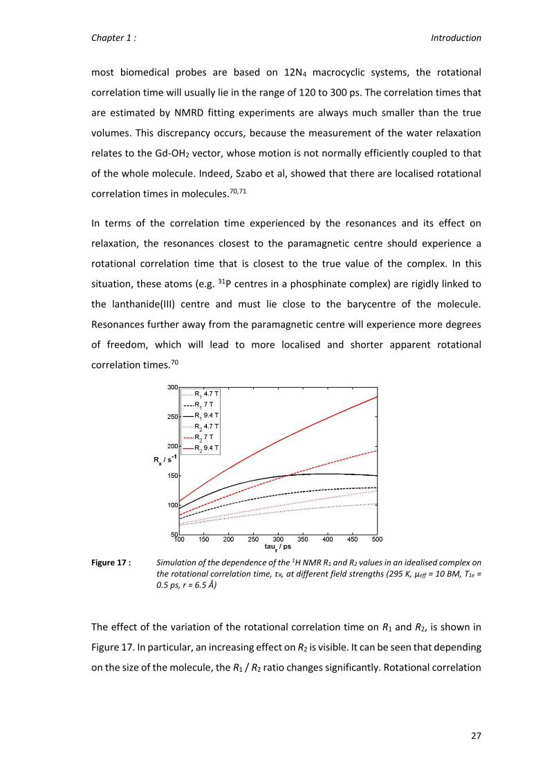
To extend the data sets, isostructural series of lanthanide(III) complexes are used, so
that the rotational correlation time and the internuclear distance can be taken as global
variables and are assumed to be the same across a complex series of lanthanides. Even
though the lanthanide contraction is present across the 4f series, the effect can be
neglected when looking at internuclear distances, as the change in ionic radius is of the
order of 0.05 Å from Tb(III) to Yb(III) and this is a relatively small change compared to
other errors.15
Scheme 1 : Structures of the isostructural series of lanthanide(III) complexes studied in this thesis.

Chapter 1 : Introduction
33
A wide range of complex series was used to gain insight into the factors that influence
the rate of electronic relaxation (Scheme 1). The complexes [Ln.L1-3] are C3 symmetric
and adopt a tricapped trigonal prismatic coordination geometry with no bound water.
They only differ in the anionic donor group (carboxylate, phosphinate and amide
respectively), creating a different ligand field at the metal centre.74
The cationic complex [Ln.L4(OH2)]3+ (from here on labelled as [Ln.L4]3+) has a hydration
number of one and adopts a C4 symmetric monocapped SAP coordination geometry.15
The phosphinate complex [Ln.L5]- also has a C4 symmetric coordination geometry.
However, it has no bound water molecule and forms a TSAP complex.75 The remaining
complexes lack Cn time-average symmetry and form a SAP coordination environment,
with the exception of [Ln.L9]+, which forms C2 symmetric SAP complexes. Again, the main
differences between these complexes are the differences between the anionic donor
groups. The series of complexes [Ln.L7], [Ln.L8] and [Ln.L10], [Ln.L11] are direct analogues
of each other and should behave similarly as only their anionic donor groups change.46,61
The main difference between the carboxylate and the phosphinate complex series,
apart from donor atom polarizability and size, is the common hydration number of one
and zero.
Some of the complexes possess heteroatoms (19F, 31P), allowing multinuclear NMR
analysis. Therefore, wherever possible, multiple resonances were analysed. The analysis
was limited to resonances at an intermediate distance to the paramagnetic
lanthanide(III) ions. Too short a distance will lead to severe line broadening and too long
a distance introduces more degrees of freedom to the resonance of interest.11
Overall, this selection of isostructural series of lanthanide complexes permits a wide
overview of electronic relaxation times, in different environments, from the
symmetrical C3 and C4 systems to the low symmetry complex series.
A few more individual complexes (e.g. [Ln.gDOTA]5-, [Tm.DOTMA]-) were analysed and
will be shown and described as appropriate.

Chapter 1 : Introduction
34
1.5.2 Investigating the pseudocontact shift
The magnetic anisotropy of lanthanide(III) complexes is another quantity that, when
modified correctly, can enhance a paramagnetic probe or contrast agent significantly.
For example, in PARACEST the sensitivity of the technique is directly linked to the shift
difference of the resonance in exchange. Investigations in the true behaviour of
magnetic susceptibility would not only benefit our understanding and design of
PARACEST agents, but also benefit in the design of paramagnetic probes for biomedical
imaging and protein tagging, as larger pseudocontact shifts are desirable in these
systems.
1.5.2.1 The limitations of Bleaney’s theory of magnetic anisotropy
Bleaney’s theory of magnetic anisotropy is widely accepted and is normally used to
estimate the pseudocontact shift of paramagnetic lanthanide(III) complexes. However,
there are a few assumptions that do not allow accurate determination of the
pseudocontact shift. First of all, a point dipole approximation is used, which is known to
be an inaccurate depiction. Binnemans et al. have carried out extensive studies on
magnetic anisotropy, and highlighted the many discrepancies of Bleaney’s theory.76
They showed that Dy(III) is not always the lanthanide(III) ion that exhibits the highest
magnetic anisotropy, as the Bleaney coefficient would indicate, but depending on the
coordination environment, Tb(III) and even Tm(III) can surpass Dy(III) in the magnitude
of magnetic anisotropy. This would indicate a much higher dependence on the ligand
field than suggested by Bleaney.77 Another of Bleaney’s initial assumptions is the
temperature independence of certain parameters. Several studies investigated the
variation of shift with T in detail, seeking to explain the deviation from the proposed
1 / T2, but no conclusive results were reached.62,76,77
Bleaney had also underestimated the ligand field contribution to the overall dipolar
shift. In his original proposal2, Bleaney assumed that the overall ligand field was of the
order of 100 cm-1 (vs 205 cm-1 for kT at 298 K) and that it would tend to be cancelled out

Chapter 1 : Introduction
35
by the (kT) term. Such a situation arises for systems with small ligand field splitting.
However, much bigger ligand fields have been observed of up to 2000 cm-1, which is of
the same order of magnitude as the splitting of the electronic energy levels due to spin-
orbit coupling. Additionally, Bleaney only considered the second rank crystal field
splitting parameters, 𝐵02 and 𝐵2
2 and ignored higher order parameters. Again, the higher
order parameters associated with multiple electrostatic interactions, may contain a
significant part of the overall crystal field. In particular, this is the case for the low
symmetry systems as the higher order parameters are likely to play an even more
important role. While the sign of the magnetic anisotropy is correctly predicted by
Bleaney’s theory, the magnitude and differences are difficult to quantify, due to the
approximations made.9,12,77
1.5.2.2 Shift behaviour in isostructural series of lanthanide(III)
complexes
In some cases it is not possible to explain the difference in the dipolar shift, by simply
looking at the relative 𝐵02 values postulated by Bleaney’s theory. An extensive study
reported by Sherry and Ren et al. showed that the experimental values of the dipolar
shift may deviate significantly from theoretical predictions.78
The isostructural series of lanthanide(III) complexes presented in Scheme 1 create the
perfect opportunity to investigate pseudocontact shift behaviour in a large series of
related systems. For resonances that are further than 4.5 Å away from the paramagnetic
centre, there is a vanishing small contact contribution that can be neglected. Comparing
a resonance to a diamagnetic analogue (e.g. Y(III)), allows the pseudocontact shift to be
estimated, independent of the contact and diamagnetic contributions.
Of course, the ionic radius of the lanthanide ions decreases across a lanthanide series
due to lanthanide contraction. This contraction will slightly change the internuclear
distance and the angle with respect to the magnetic principal axis. However, the

Chapter 1 : Introduction
36
resonances under investigation each possess big pseudocontact shifts and the
differences due to these changes will be small.
A numerical method can be employed to predict the shift by Bleaney’s theory, by
comparing the shift values for every complex in a series to the value of the Yb(III)
analogue. The Yb(III) ion possess the smallest magnetic susceptibility among all the
lanthanides in the second half of the 4f series and it is generally regarded as the
lanthanide(III) ion which is best characterised by Bleaney’s theory.10,76 Additionally, a
linear correlation should be observed between the values of the Bleaney constant and
the true pseudocontact shift.
The complexes in Scheme 1 also present a variety of different types of symmetry. In Cn
symmetry, the crystal field splitting is dominated by 𝐵02, which can be estimated for
every complex using the method developed by Binnemans et al.10 However, the crystal
field splitting is expected to be much more complicated for the low symmetry systems,
due to the influence of the higher order parameters. These higher order terms are not
considered by Bleaney’s theory. Consequently, these low symmetry systems should
show interesting behaviour in terms of the pseudocontact shift.

Chapter 2: Electronic relaxation times through analysis of nuclear relaxation rates
37
2. Electronic relaxation times estimated through
analysis of nuclear relaxation rates

Chapter 2: Electronic relaxation times through analysis of nuclear relaxation rates
38
By measuring nuclear relaxation rates of ligand resonances as a function of the magnetic
field, it is possible to estimate the electronic relaxation times of lanthanide(III)
complexes. The nuclear relaxation data is fitted to the Solomon-Bloembergen Morgan
equations, obtaining estimates of, not only the electronic relaxation times, but also the
internuclear distances, the effective magnetic moments and the rotational correlation
times.
2.1 Parameters influencing the nuclear relaxation rates
The method of fitting the nuclear relaxation rates at different fields was developed by
Kuprov and Parker in 2009.23 The measured nuclear relaxation rates were measured at
4.7, 9.4, 11.7, 14.1 and 16.5 Tesla and can be fitted to the Solomon-Bloembergen
Morgan equations for the longitudinal relaxation rate, R1 (equation 4) or the transverse
relaxation rate, R2 (equation 5):
𝑅1 =2
15 (
µ0
4π)
2
γN
2 𝑔𝐿𝑛2 µ𝐵
2 𝐽 (𝐽 + 1)
𝑟6 [3
𝑇1𝑒
1 + 𝜔𝑁2 𝑇1𝑒
2 + 7𝑇2𝑒
1 + 𝜔𝑒2 𝑇2𝑒
2 ]
+2
5(
μ0
4π)
2 𝜔𝑁2 µ𝑒𝑓𝑓
4
(3kB𝑇)2 𝑟6[3
𝜏𝑟
1 + 𝜔𝑁2 𝜏𝑟
2] (4)
𝑅2 =2
15 (
µ0
4π)
2
γN
2 𝑔𝐿𝑛2 µ𝐵
2 𝐽 (𝐽 + 1)
𝑟6 [2𝑇1𝑒
3
2
𝑇1𝑒
1 + 𝜔𝑁2 𝑇1𝑒
2 +13
2
𝑇2𝑒
1 + 𝜔𝑒2 𝑇2𝑒
2 ]
+2
5(
μ0
4π)
2 𝜔𝑁2 µ𝑒𝑓𝑓
4
(3kB𝑇)2 𝑟6[2𝜏𝑟
3
2
𝜏𝑟
1 + 𝜔𝑁2 𝜏𝑟
2] (5)
There are a few underlying assumptions in SBM theory. Similar to Bleaney’s theory of
magnetic anisotropy, a point-dipole approximation is assumed. Additionally, the zero-
field splitting (ZFS) of the energy levels is neglected in the dipolar term. However, Bertini
and Luchinat28 proposed a variant of the SBM equations that incorporated the static

Chapter 2: Electronic relaxation times through analysis of nuclear relaxation rates
39
ZFS. Inclusion of this modified term led to electronic relaxation times 2 -3 times faster
than those calculated previously.
As can been seen in equation 4 and 5, the two terms (dipolar and Curie) are additive
and independent of each other. Therefore, no cross-relaxation is allowed.
Lastly, the rotational correlation time is treated as isotropic and is assumed to be the
same for each resonance. However, Szabo et al.70,71 introduced the effect of localised
rotational correlation times, which might also have an effect here and will be discussed
later (chapter 2.2.1.2).
The sets of measured relaxation rates were fitted using a Levenberg-Marquardt
minimisation technique, which allows ‘fixing’ of individual parameters to specific values,
thereby taking the parameter out of the estimation process. By fixing a parameter the
minimisation procedure is greatly simplified. Of course, it is necessary to know a
reasonable value for the fixed parameter with confidence. For example, the
temperature during the measurement is a fixed quantity, as it can easily be controlled
and was measured accurately during each measurement in this work (see below, section
2.1.2).
The Levenberg-Marquardt minimisation technique cannot distinguish between global
and local minima. Therefore, the quality of the initial estimates of the parameters
involved in the fitting is important, to avoid being trapped in a false, local minimum. The
parameters that need to be estimated for the fitting are: the internuclear distance, r,
the rotational correlation time, τR, the effective magnetic moment, µeff, and the
electronic relaxation time, T1e.
The experimental relaxation data can either be fitted on a peak by peak basis (single
resonance fitting) or a common resonance across the isostructural series can be fitted
on a global level (global fitting). The method is applicable for analysis of R1 and R2 data
sets, but in this discussion the focus will be on the analysis of the longitudinal relaxation
rates, R1. The nuclear relaxation rates of the ligand resonances of eleven isostructural
series of lanthanide(III) complexes and a few more connected complexes were

Chapter 2: Electronic relaxation times through analysis of nuclear relaxation rates
40
measured for the Tb(III), Dy(III), Ho(III), Er(III), Tm(III) and Yb(III) analogues. In some
cases data for the Eu(III) analogues were also analysed (Scheme 2).
Scheme 2 : Structures of the isostructural series of lanthanide(III) complexes studied in this thesis.
Various techniques were used to estimate the parameters involved in the fitting of the
nuclear relaxation rates. The electronic relaxation times of these complexes are, of
course, unknown, but can be roughly estimated from prior literature studies. The
observed range of the electronic relaxation times is thought to be between 0.1 and

Chapter 2: Electronic relaxation times through analysis of nuclear relaxation rates
41
1 ps. It is expected that the electronic relaxation times will vary according to the nature
of the lanthanide(III) ion. From the reported literature, initial estimates can be obtained
and it was noted that Tb(III) and Dy(III) complexes gave higher electronic relaxation
times than the remaining lanthanide(III) ions.28,66–68,72
The effective magnetic moment, µeff, is commonly regarded as being independent of
the coordination environment of the lanthanide(III) ions and, therefore, can be
estimated easily from literature studies.23,79 These values are most commonly measured
from magnetic susceptibilities of solid-state samples.12
The global fitting procedure analyses common ligand resonances within an isostructural
series of lanthanide(III) complexes, but requires a few assumptions to be made. First of
all, the internuclear distances across a series are assumed not to change within their
respective errors. It is appreciated that the lanthanide contraction means that the ionic
radius of the lanthanide(III) ion decreases, but the expected decrease is contained
within the estimated errors. A similar concept applies to the molecular volume of a
complex and, therefore, its rotational correlation time. The internuclear distances, r,
can be estimated from solid-state X-ray diffraction structures. There is often a slight
difference between the solid and solution state structures, due to the greater
conformational mobility in solution, but the distances obtained from the crystal
structures provide the best initial estimates. The origin of differences between solid and
solution-state estimates is discussed further in section 2.1.2.
Figure 20: Views of the X-ray structures of the two diasteroisomers of [Eu.L3]3+: S-Δ-(λλλ) (left) and R-Λ-(δδδ) right (120 K).74

Chapter 2: Electronic relaxation times through analysis of nuclear relaxation rates
42
Most of the complexes presented here have published X-ray crystallographic structures
available. Structures of [Ln.L1]80, [Ln.L2]29 and [Ln.L5]-75 have been reported previously.
The series of [Ln.L3]3+ complexes were published74 during the course of the work
presented here (Figure 20). Additionally, X-ray structures are available for almost the
whole series of lanthanide(III) complexes of [Ln.L4]3+.15
An isostructural series of complexes based on crystallographic analyses provides an
excellent opportunity to investigate the effect of the lanthanide contraction. Due to the
monotonic decrease in ionic radius, it is expected that the internuclear distances will
decrease across the series. The whole 4f series was investigated, but only the second
half, from Tb(III) to Yb(III), is of interest in this study (Table 5).
Table 5: Variation of the internuclear distance, r, in X-ray structures across the series of lanthanide(III) complexes of [Ln.L4]3+ (120 K).19
Ln3+ r / Å
Hax Heq Hax’ Heq’ CHCO’ CHCO
Pr 3.79 4.43 3.75 4.44 3.71 4.36 Nd 3.77 4.41 3.73 4.42 3.70 4.33 Sm 3.74 4.38 3.71 4.40 3.69 4.31 Eu 3.75 4.38 3.71 4.40 3.66 4.31 Gd 3.74 4.38 3.70 4.39 3.67 4.28 Dy 3.73 4.37 3.69 4.37 3.67 4.26 Yb 3.68 4.35 3.65 4.33 3.55 4.24
While the internuclear distances across a whole series (La(III) to Yb(III)) can decrease by
up to 0.1 Å, the distances within the latter half of the 4f series decrease by less than
0.05 Å.81 The limited decrease of the internuclear distance, r, allows it to be used as a
global fitting variable across a series from Tb(III) to Yb(III).
This type of analysis can be extended to the estimates of the rotational correlation time,
τR, as it is dependent on the overall size of the complex. According to the Stokes-Einstein

Chapter 2: Electronic relaxation times through analysis of nuclear relaxation rates
43
Law (equation 6), the main factor determining τR is the hydrodynamic radius, rH,
(Figure 21).69
𝜏𝑅 = 1
6𝐷=
4𝜋𝑟𝐻3𝜂
3𝑘𝑇 (6)
where D is the rotational diffusion constant and η is the viscosity of the solvent.
Figure 21: Illustration of the X-ray structure of [Gd.L4]3+ with the estimation of the hydrodynamic radius highlighted (120 K).19
Assuming a spherical model, it is possible to estimate the rotational correlation time, τR,
of a complex series by measuring the distance of the nucleus furthest away from the
paramagnetic centre and calculating the volume of the model sphere. The measured
difference in the hydrodynamic radius from [Gd.L4]3+ (7.15 Å) to [Yb.L4]3+ (7.04 Å) was in
a similar range to the decrease in the internuclear distance and contributes to an overall
variation of the rotational correlation time of less than 5%. The limited decrease of the
hydrodynamic radius associated with the lanthanide contraction permits the use of a
common τR parameter, across the latter half of the series.

Chapter 2: Electronic relaxation times through analysis of nuclear relaxation rates
44
2.1.1 Relaxation behaviour in isostructural series of lanthanide(III)
complexes
A variety of parameters influence the nuclear relaxation rates of a paramagnetic
lanthanide(III) complex. In an isostructural series, however, the majority of parameters
do not change across the series. As discussed above, the internuclear distance and the
rotational correlation times can safely be assumed to be constant. The two main
parameters that change between the lanthanide(III) ions are the effective magnetic
moment, µeff, and the electronic relaxation time, T1e. Each of these parameters is
important in the Solomon-Bloembergen Morgan equations via the Curie and the dipolar
term respectively.
In the relaxation experiment undertaken here, the nuclear relaxation rates are
measured as a function of the magnetic field, ranging from relatively low magnetic field
strengths (4.7 – 9.4 T) to the high field range (9.4 – 16.5 T). Due to the dependence of
the Curie term on 𝜇𝑒𝑓𝑓4 𝜔𝑁
2 , the Curie terms becomes increasingly important at higher
magnetic field strengths. Therefore, at higher field strengths it can be expected that the
nuclear relaxation rates follow the order of µeff. At lower magnetic field strengths, it is
expected for T1e to have a dominant influence on the nuclear relaxation rates, which
might alter the order of nuclear relaxation rates from the one observed at the higher
field strengths.
Table 6 : Overview of the measured 1H relaxation rate, R1, of and the observed shift of the CH3 resonances (9.4 T) of [Ln.L4]3+ (295 K, D2O).
Ln3+ δH / ppm R1
a / s-1
4.7 T 9.4 T 11.7 T 14.1 T 16.5 T
Tb 20.8 66 101 114 125 131
Dy 24.4 76 126 144 160 171
Ho 12.9 52 97 115 130 137
Er -4.5 30 56 69 78 85
Tm -13.1 18 28 33 36 38
Yb -3.9 7.6 6.8 7.1 7.2 7.2 aThe experimental error estimated for the measurement of R1 values is less than 5%.

Chapter 2: Electronic relaxation times through analysis of nuclear relaxation rates
45
The differences in the nuclear relaxation rates between the lanthanide(III) ions in an
isostructural series are due to the variation of values for T1e and µeff of the different
lanthanide(III) ions. Table 6 shows an overview of the relaxation and shift behaviour for
the CH3 resonance of [Ln.L4]3+. At high magnetic field strengths, the order of the nuclear
relaxation rates follows the order of magnetic moments ([Dy, Ho] > Tb > Er > Tm >> Yb).
The only exceptions are the values of Tb(III) and Ho(III), which are close despite the
differences of more than 1 BM in µeff. At lower magnetic field strengths, the order
dictated by the effective magnetic moment can change since the nuclear relaxation
rates are influenced more strongly by the electronic relaxation times. Measuring the
electronic relaxation times will provide a better understating of the nuclear relaxation
behaviour at lower magnetic field strengths. The issue is of particular relevance to
selecting probes in biomedical imaging, where fields of 1.5 and 3 T are commonly used.
Figure 22 highlights the R1 vs T1e behaviour from the simulation shown earlier (Figure
16), clearly showing the key role played by T1e variation at 1.5 to 3 T in the modulation
of R1.
Figure 22 : Simulation of the dependence of R1 on T1e at a variety of fields for an idealised lanthanide(III) probe (295 K, µeff = 10 BM, r = 6.5 Å, τR = 250 ps).
2.1.1.1 Characterisation by relaxation and shift behaviour
In an isostructural series, it is important to confidently assign the 1H NMR resonances to
allow the use of the global fitting procedure. Due to the distance dependence of the
longitudinal (R1) and transverse (R2) relaxation rates, it is easy to map the structure of a

Chapter 2: Electronic relaxation times through analysis of nuclear relaxation rates
46
lanthanide(III) complex by considering their relative relaxation enhancements and by
reference to published X-ray structures (Figure 15).
The effect of the internuclear distance on the nuclear relaxation rates is still constrained
by the lanthanide(III) ion, its associated effective magnetic moment and the individual
electronic relaxation times. Therefore, the steepness of the measured distance
dependence varies according to the nature of the lanthanide(III) ion. However, in a
comparative analysis of the relaxation rates across different lanthanide(III) ions, it is
possible to differentiate between different resonances, by virtue of their shift and
relative relaxation rates.
The Yb(III) ion has a small effective magnetic moment (4.5 BM) and, coupled with low
estimated electronic relaxation times, low nuclear relaxation rates are observed. The
slow transverse relaxation rates, together with a smaller observed shift range than for
the other lanthanide(III) ions, make a full characterisation of the 1H NMR spectrum of a
Yb(III) complex relatively straightforward, which is normally not possible for the other
lanthanide(III) ions.
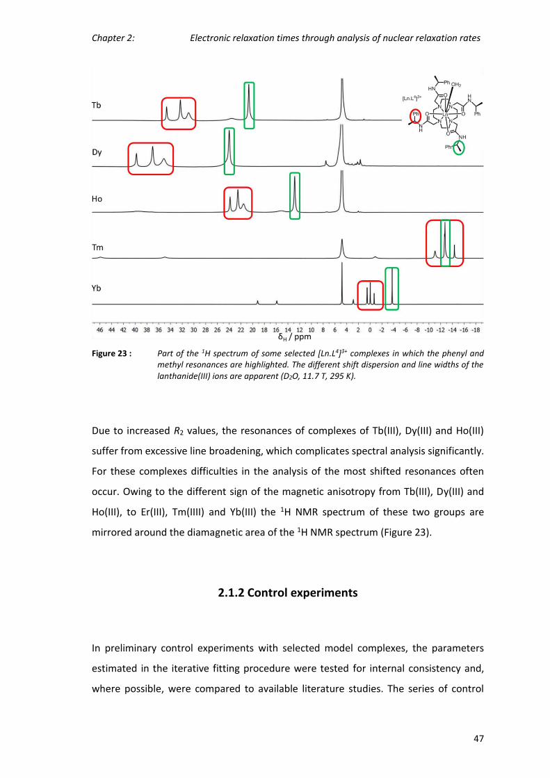
Chapter 2: Electronic relaxation times through analysis of nuclear relaxation rates
47
Figure 23 : Part of the 1H spectrum of some selected [Ln.L4]3+ complexes in which the phenyl and methyl resonances are highlighted. The different shift dispersion and line widths of the lanthanide(III) ions are apparent (D2O, 11.7 T, 295 K).
Due to increased R2 values, the resonances of complexes of Tb(III), Dy(III) and Ho(III)
suffer from excessive line broadening, which complicates spectral analysis significantly.
For these complexes difficulties in the analysis of the most shifted resonances often
occur. Owing to the different sign of the magnetic anisotropy from Tb(III), Dy(III) and
Ho(III), to Er(III), Tm(IIII) and Yb(III) the 1H NMR spectrum of these two groups are
mirrored around the diamagnetic area of the 1H NMR spectrum (Figure 23).
2.1.2 Control experiments
In preliminary control experiments with selected model complexes, the parameters
estimated in the iterative fitting procedure were tested for internal consistency and,
where possible, were compared to available literature studies. The series of control

Chapter 2: Electronic relaxation times through analysis of nuclear relaxation rates
48
experiments include investigations into the estimated values of the effective magnetic
moment, the rotational correlation time and the internuclear distance.
2.1.2.1 Effect of the temperature
In the standard experiment, the nuclear relaxation rates were measured at constant
temperature across all five different fields (295 K). This is important as in the Solomon-
Bloembergen Morgan equations (4 and 5) there are a few parameters that are
influenced by the temperature. There is a direct dependence of the nuclear relaxation
rates to temperature in the Curie term (1 / T2), but the rotational correlation time is also
influenced by the temperature (1 / T).
Figure 24: Variation of the nuclear relaxation rate, R1, of the 31P resonance of [Tm.L2] with the temperature(16.5 T, CD3OD).
The nuclear relaxation rate of the 31P resonance of [Tm.L2] was measured at different
temperatures. A linear variation was found at 16.5 Tesla between R1 and 1 / T2 (Figure
24). However, the magnetic field strength needs to be considered carefully in this study,
due to the increasing influence of the Curie term at higher magnetic field strengths.
390
400
410
420
430
440
450
460
470
0,1090 0,1100 0,1110 0,1120 0,1130 0,1140 0,1150 0,1160
R1
/ s-1
T-2 x 10⁻³

Chapter 2: Electronic relaxation times through analysis of nuclear relaxation rates
49
2.1.2.2 Effect of the internuclear distance
The fitting algorithm can be modified to allow fixing of individual parameters. The
possibilities of fixing the effective magnetic moment, the rotational correlation and the
internuclear distance were investigated in order to minimise the errors of the fitting
procedure. Fixing the effective magnetic moment allows calculation of the electronic
relaxation times, the internuclear distances and the rotational correlation times. To
show the validity and accuracy of the estimated values, the internuclear distances can
be compared to values found in the X-ray crystallographic structures. Confidence in
these values will also establish confidence in the estimated values of the electronic
relaxation times.
For the C3 symmetric isostructural series of complexes based on triazacyclononane
([Ln.L1-3]), the relaxation rate data for each separate common resonance were
minimised, holding the relevant µeff to their literature values and varying T1e, τR and r.
A very good agreement was found between the internuclear distances estimated
through single resonance fitting and the X-ray data (Table 7).

Chapter 2: Electronic relaxation times through analysis of nuclear relaxation rates
50
Table 7: Calculated average internuclear distances, r, across the C3 complex series using single fitting with a fixed µeff (295 K, CD3OD, [Ln.L1] in D2O) compared with the X-ray data (120 K).
Calculated r / Å X-ray dataa
[Ln.L1] [Ln.L2] [Ln.L3]3+ [Ln.L2] [Ln.L3]3+
Hax 4.33 ±0.14 4.34 ±0.10 4.45 ±0.02 4.12 4.06
Hax’ 3.78 ±0.10 3.97 ±0.01 3.87 ±0.01 3.45 3.42
Heq 4.49 ±0.03 4.54 ±0.01 4.55 ±0.02 4.30 4.28
Heq’ 4.40 ±0.03 4.55 ±0.01 4.53 ±0.02 4.30 4.23
pyCHN 4.45 ±0.10 4.45 ±0.10 4.71 ±0.01 4.30 4.31
pyCHN’ 3.92 ±0.10 3.48 ±0.04 3.50 ±0.01 3.50 3.50
pyH3 5.56 ±0.01 6.00 ±0.20 5.50 ±0.03 5.53 5.45
pyH4 6.33 ±0.02 7.33 ±0.40 6.43 ±0.01 6.36 6.26
pyH5 5.40 ±0.20 5.99 ±0.20 5.72 ±0.01 5.59 5.48 aObtained from [29,74,80].
Table 7 shows the average values of the internuclear distance over the isostructural
series of [Ln.L1], [Ln.L2] and [Ln.L3]3+. A slight deviation was expected due to the
differences between solid and solution state structures. The only resonances that seem
to deviate from the expected value are the pyH4 resonance of [Ln.L2] and the pyCHN’
value of [Ln.L1], which can only be attributed to an error in the R1 measurements.
Overall, the difference between the estimation through the fitting procedure and the X-
ray structures gives considerable confidence in the single resonance fitting method with
a fixed value for µeff.

Chapter 2: Electronic relaxation times through analysis of nuclear relaxation rates
51
Table 8: Calculated average internuclear distances, r, across the [Ln.L4]3+ series, using a single fitting method with a fixed µeff (295 K, D2O) compared to the X-ray crystallographic data (120 K).
r / Åa X-raya
Hax 3.90 ±0.01 3.73
Hax’ 3.57 ±0.01 3.69
Heq 4.48 ±0.11 4.37
Heq’ 4.48 ±0.10 4.37
CHCO 4.40 ±0.19 4.26
CHCO’ 3.75 ±0.01 3.67 aObtained from [19]
A similar comparative analysis was undertaken for the [Ln.L4]3+ systems. Again, the
estimated distances are in very good agreement with the solid-state data. The estimated
distances for the ring protons do not change significantly for the remaining 12N4 based
complexes ([Ln.L5]- to [Ln.L11], see Appendix 2).
2.1.2.3 Confirmation of the variation of R1 with r
To check the internal consistency of the estimated distances, the nuclear relaxation
rates of sets of individual resonances in a given complex were compared to the X-ray
crystallographic distances. Over multiple resonances, the direct dependence of the
nuclear relaxation rates on 1 / r6 should be visible for all resonances analysed in a given
lanthanide(III) complex. The relaxation rates for five different [Ln.L2] complexes were
measured (295 K, 4.7 T) and the variation of R1 with the internuclear distance, r taken
from the X-ray structures was analysed (Figure 25). The intercept of each graph should
go through 1 s-1, which is the theoretical diamagnetic contribution.

Chapter 2: Electronic relaxation times through analysis of nuclear relaxation rates
52
Figure 25 : Dependence of the relaxation rate, R1, on the lanthanide to 1H internuclear distance, r, taken from X-ray structures for the [Ln.L2] series (295 K, CD3OD).82
Figure 25 shows that the nuclear relaxation rates and the estimated internuclear
distances faithfully follow the expected dependence of 1/r6, for a variety of
lanthanide(III) ions.
2.1.2.4 Variation of τR and solvent viscosity
The second parameter that is calculated in any single resonance fitting procedure with
a fixed µeff, is the rotational correlation time, τR. The solubility of [Ln.L4]3+ allows the
analysis of the nuclear relaxation rates in different solvents. The different viscosities of
solvents will give rise to different rotational correlation times and, consequently, lead
to modulation of the nuclear relaxation rates. The 1H NMR relaxation rates for ligand

Chapter 2: Electronic relaxation times through analysis of nuclear relaxation rates
53
resonances were measured in deuterated water, methanol and acetonitrile (Table 9,
and Appendix 2, SI-Table 30 -31).
Table 9 : Variation of calculated T1e and τR values with different solvents for [Ln.L4]3+, at 295 K using a single fitting procedure with a fixed value of µeff.
Ln3+ D2O CD3OD MeCN
τR / ps τR / ps τR / ps
Tba 340.0 257.0 184.0
Dy 329.0 248.8 x
Ho 359.0 257.0 x
Tm 381.0 265.0 x
Yb 343.1 237.9 139.0
Total τR 350 ±28 253.1 ±17 161.5 ±12
ηrel 1.00 0.60 0.36 aThe τR values are an average of at least 6 measured resonance per lanthanide(III) ion., with a standard deviation of 10 ps in each case.
The estimated internuclear distances were within their respective errors and the fitted
electronic relaxation times were also independent of the nature of the solvents. The
rotational correlation time is the only parameter that changes between the three
measurements and it followed the trends of the viscosity relatively well.
In the global fitting procedure a fixed value for the internuclear distance is used to
minimise the error of the calculations. The agreement between the solid and solution
state structures was shown above, which allows for the internuclear distances to be
fixed to the values from the X-ray crystallographic studies. The effective magnetic
moments are calculated using this method, and the estimated values are close to the
literature values. An extensive analysis of the calculated effective magnetic moments
will be given in chapter 4 and in the individual analyses of the complexes below (section
3.3.1 to 3.3.3).
These control experiments substantiate the validity of this experimental technique. The
two computational methods used here: single resonance fitting using a fixed µeff value
and global fitting using a fixed value of r were each shown to give reasonably accurate
values for each parameter.

Chapter 2: Electronic relaxation times through analysis of nuclear relaxation rates
54
2.1.2.5 Error Analysis in R1 and determination of fitting errors
Each R1 relaxation measurement was repeated at least three times and the mean value
recorded. The number of transients used in the measurements was determined by the
signal-to-noise ratio and therefore primarily by the concentration of the complex
solution and the linewidth of the resonance of interest. This concentration was kept
constant across the different experiments and was typically in the range of 0.2 to 1 mM.
In each case, the signal analysed was fully recovered during the inversion-recovery
sequence.
An experiment was performed to calculate the error associated with the temperature
variation between the spectrometers. The relaxation rate of [Tm.L2] was measured at
five different temperatures (295 – 303 K in 2 K steps). For each measurement, the
temperature was also determined using the temperature calibration sample (ethylene
glycol). According to the Solomon-Bloembergen Morgan equations, the temperature
dependence of the relaxation rate, R1, is 1 / T2. At a variation of 0.5 K the error was
found to be less than 1.3 %. This was assumed to be similar for each complex studied
(calculated from Figure 24).
An error analysis was undertaken to determine the fitting errors. The experimental
errors of the measured relaxation rates were combined and used to perturb the
relaxation rates for each complex at each field. These perturbed rates, together with
the unperturbed relaxation rates were used in a statistical error analysis to obtain the
error values for the individual parameters (µeff, r, τr and T1e) estimated in the fitting
process.

Chapter 2: Electronic relaxation times through analysis of nuclear relaxation rates
55
Table 10 : Variation of the fitting results when perturbing the experimental nuclear relaxation data within their respective errors for the global fitting of the Heq’ resonance of [Ln.L4]3+ (295 K, D2O).
µeff / BM τR /
ps T1e / ps
Eu Tb Dy Ho Tm Yb Eu Tb Dy Ho Tm Yb
2.990 8.909 10.325 9.951 7.578 4.344 335.3 0.141 0.564 0.382 0.281 0.262 0.200
2.836 8.898 10.320 9.946 7.568 4.311 334.9 0.101 0.567 0.380 0.278 0.256 0.183
2.979 8.917 10.330 9.956 7.587 4.379 335.6 0.176 0.568 0.386 0.285 0.267 0.216
2.865 8.903 10.323 9.949 7.574 4.328 335.3 0.122 0.568 0.381 0.280 0.259 0.192
2.937 8.911 10.327 9.953 7.592 4.361 335.4 0.159 0.569 0.384 0.283 0.265 0.208
An example for the perturbations and the resulting estimated parameters is given in
Table 10.
2.2 Estimated electronic relaxation time, T1e data
The nuclear relaxation rates of selected ligand resonances, in each series of
lanthanide(III) complexes, were measured at five different field strengths. Using the
fitting methods described previously (section 2.1), up to four parameters were
estimated (µeff, τR, r and T1e) for the lanthanide(III) ions of eleven different complexes.
However, in most cases, some parameters were ‘fixed’ to a set value and were,
therefore, taken out of the minimisation process. The main procedure for estimating
the parameters of the Solomon-Bloembergen Morgan equation involved the global
fitting of one or more common resonances across the isostructural series of
lanthanide(III) complexes. The analysis has been limited to the very fast relaxing
lanthanide(III) ions: Tb(III), Dy(III), Ho(III), Er(III), Tm(III) and Yb(III). The main motivation
for this analysis is the estimation of the electronic relaxation times, T1e, of individual
lanthanide(III) complexes in a given isostructural series.
Details of the physical basis of electronic relaxation are uncertain. In previous studies, it
was postulated that the zero field splitting (ZFS) of the electronic energy levels due to
the J energy levels and the ligand field were in some way responsible for the

Chapter 2: Electronic relaxation times through analysis of nuclear relaxation rates
56
modulation.28,66,68,82 In addition, it was proposed by Bertini et al.28 that the modulation
of the nuclear relaxation rates by the electronic relaxation arises from solvent collisions
that disturb the ligand field of the complex. Such a process is limited by vibrational
motion and therefore sets the lower limit for the electronic relaxation times to 0.1 ps.
The expected range of electronic relaxation times can be estimated, from prior
literature studies, is in the range of 0.1 ps to 1 ps.
An overview for all estimated parameters using the global fitting procedure with a fixed
value of the internuclear distance, r, from X-ray crystallographic data can be found in
Table 11 and 12. A brief summary of how the estimated values were obtained in section
2.1. Hereafter, the data for each series is divided into different categories, for more
specific comment and analysis.

Chapter 2: Electronic relaxation times through analysis of nuclear relaxation rates
57
Table 11 : Calculated electronic relaxation times, T1e ,a effective magnetic moments, µeff and rotational correlation times, τr derived using global fitting with a fixed internuclear distance, r (295K, [Ln.L1], [Ln.L4]3+, [Ln.L5]- in D2O, [Ln.L2,3] in CD3OD.
Ln3+
[Ln.L1] [Ln.L2] [Ln.L3]3+ [Ln.L4]3+ [Ln.L5]-
1H 1H 31P 1H 1H 1H
µeff/ BM T1e / ps µeff/ BM T1e / ps µeff/ BM T1e / ps µeff/ BM T1e / ps µeff/ BM T1e / ps µeff/ BM T1e / ps
Tb 9.65 ±0.02 0.26 ±0.03 8.76±0.03 0.21 ±0.04 8.75 ±0.04 0.28 ±0.01 9.81 ±0.03 0.29 ±0.03 9.23 ±0.01 0.57 ±0.01 9.64 ±0.01 0.31 ±0.01
Dy 10.47 ±0.01 0.28 ±0.02 9.50 ±0.03 0.32 ±0.03 9.72 ±0.05 0.26 ±0.01 9.92 ±0.03 0.25 ±0.03 10.30 ±0.01 0.42 ±0.01 10.56 ±0.01 0.41 ±0.01
Ho 10.44 ±0.01 0.17 ±0.02 10.48 ±0.01 0.11 ±0.02 9.39 ±0.04 0.13 ±0.01 10.32 ±0.02 0.23 ±0.03 9.91 ±0.01 0.31 ±0.01 10.29 ±0.01 0.31 ±0.01
Er 9.23 ±0.02 0.23 ±0.03 9.55 ±0.02 0.26 ±0.03 8.50 ±0.04 0.31 ±0.01 8.88 ±0.03 0.26 ±0.04 X X 9.48 ±0.01 0.57 ±0.01
Tm 7.43 ±0.01 0.08 ±0.02 8.21 ±0.03 0.09 ±0.04 6.76 ±0.03 0.06 ±0.02 7.77 ±0.02 0.13 ±0.03 7.57 ±0.01 0.28 ±0.01 9.07 ±0.01 0.83 ±0.01
Yb 4.27 ±0.02 0.09 ±0.04 4.72 ±0.03 0.12 ±0.06 3.84 ±0.03 0.07 ±0.01 4.55 ±0.04 0.14 ±0.04 4.34 ±0.03 0.21 ±0.02 4.27 ±0.05 0.24 ±0.02
τR / ps 132 ±1 186 ±6 328 ±15 184 ±1 293 ±1 230 ±1
aThe estimates of the following resonances were analysed : [Ln.L1] = pyH3,4, [Ln.L2] =Hax, Hax’,, pyH3,5, [Ln.L3]3+ = pyH3,4, [Ln.L4]3+ = Heq, Heq’, [Ln.L5]- = Heq, Heq’, Me.

Chapter 2: Electronic relaxation times through analysis of nuclear relaxation rates
58
Table 12: Calculated electronic relaxation times, T1e ,a effective magnetic moments, µeff and rotational correlation times, τr using global fitting with a fixed internuclear distance, r, for the lower symmetry complexes[Ln.L6-11] (295 K, D2O).
Ln3+
[Ln.L6] [Ln.L7] [Ln.L8] [Ln.L9]+ [Ln.L10] [Ln.L11]
1H+19F 1H 1H 1H 1H 1H
µeff/ BM T1e / ps µeff/ BM T1e / ps µeff/ BM T1e / ps µeff/ BM T1e / ps µeff/ BM T1e / ps µeff/ BM T1e / ps
Tb 9.23 ±0.04 0.44 ±0.03 9.89 ±0.03 0.71 ±0.05 8.74 ±0.06 0.57 ±0.04 10.23 ±0.03 0.91 ±0.04 9.47 ±0.02 0.55 ±0.02 9.63 ±0.01 0.69 ±0.01
Dy 9.88 ±0.03 0.40 ±0.02 10.44 ±0.03 0.55 ±0.03 9.44 ±0.05 0.45 ±0.03 10.78 ±0.03 0.88 ±0.04 10.00 ±0.01 0.43 ±0.01 9.80 ±0.01 0.47 ±0.03
Ho 9.74 ±0.03 0.33 ±0.02 10.02 ±0.02 0.26 ±0.03 9.73 ±0.04 0.39 ±0.04 9.97 ±0.03 0.24 ±0.02 9.97 ±0.01 0.19 ±0.01 10.67 ±0.01 0.48 ±0.03
Er 9.58 ±0.03 0.63 ±0.03 9.18 ±0.02 0.17 ±0.04 9.62 ±0.04 0.97 ±0.06 X X 9.30 ±0.01 0.12 ±0.01 9.45 ±0.01 0.62 ±0.02
Tm 8.21 ±0.03 0.30 ±0.03 8.21 ±0.06 0.40 ±0.03 9.36 ±0.05 0.48 ±0.03 7.80 ±0.04 0.15 ±0.05 8.02 ±0.01 0.26 ±0.02 7.50 ±0.01 0.32 ±0.02
Yb 4.55 ±0.12 0.36 ±0.04 4.56 ±0.07 0.28 ±0.03 4.57 ±0.07 0.51 ±0.03 4.67 ±0.23 0.14 ±0.04 4.65 ±0.03 0.15 ±0.03 X X
τR / ps 260 ±2 196 ±4 263 ±4 288 ±4 182 ±1 227 ±1
aThe following resonances were analysed : [Ln.L6] = CF3, Me, [Ln.L7,8,9] = tBu, [Ln.L10] = pyH6, Heq, Heq’, [Ln.L11] = Me

Chapter 2: Electronic relaxation times through analysis of nuclear relaxation rates
59
The large amount of data presented in Table 11 and 12 is difficult to digest. However, a
few general observations can be made first.
Interestingly, the range of T1e values experienced by a lanthanide(III) ion across all the
isostructural series is larger than the range of T1e values seen within a particular
isostructural series. In other words, the coordination environment of the lanthanide(III)
ion seems to have an bigger effect on T1e than the nature of the individual lanthanide(III)
ion. These differences can be attributed to the change in the ligand field between the
isostructural series. Therefore, in some cases, ligand design has a bigger impact on the
electronic relaxation times than lanthanide(III) ion selection.
The assumption of a correlation between the ligand field and the electronic relaxation
times provides a starting point for this discussion. The lanthanide series [Ln.L1] to [Ln.L11]
were categorised by their dependence on the crystal field splitting parameters, 𝐵𝑞𝑘.
These were estimated using the emission spectra of the Eu(III) analogue of each
analysed series. The method proposed by Binnemans et al.9 allows the analysis of the
splitting of the ΔJ = 1 band to estimate the second order crystal field splitting parameter
𝐵02. There are other parameters influencing the crystal field (e.g. 𝐵0
4 and 𝐵06), but only
the second rank parameter can be estimated easily.9,10 It has been found that 𝐵02 > 𝐵2
2
for these systems reported to date.83
In the axially symmetric systems ([Ln.L1-5]), the second order crystal field splitting
parameters will be the dominant term in the observed crystal field splitting of a
complex.10 Comparing the differences between 𝐵02 and the estimated value of the
electronic relaxation times of the lanthanide(III) in isostructural series of [Ln.L1-5] should
indicate how well the parameters correlate. In the other systems ([Ln.L6-11]), the higher
order parameters are more influential due to the reduced symmetry, which makes a
direct comparison of 𝐵02 difficult, but does allow for an assessment of the possible role
of the higher order parameters in more detail overall.
𝛿𝑝𝑠𝑒𝑢𝑑𝑜 = 𝐶𝐽𝜇𝐵
2
60 (𝑘𝑇)2[(3𝑐𝑜𝑠2𝜃 − 1)
𝑟3𝐵0
2 + √6(𝑠𝑖𝑛2𝑐𝑜𝑠2𝜑)
𝑟3𝐵2
2 ] (2)

Chapter 2: Electronic relaxation times through analysis of nuclear relaxation rates
60
Additionally, the overall crystal field splitting can be estimated by comparing the NMR
observed shift range, e.g. in the 1H NMR spectrum of each complex. According to
Bleaney’s theory of magnetic anisotropy (equation 2), the pseudocontact shift is directly
proportional to the second order crystal field splitting parameters, 𝐵02 and 𝐵2
2. The
influence is highlighted in Figure 26, which shows how the ligand field variation leads to
an increase in the shift range of the Yb(III) analogue of [Ln.L1-3].
Figure 26 : 1H NMR spectrum of [Yb.L1] (upper), [Yb.L2] and [Yb.L3]3+ (lower) showing the variation
of shift dispersion with 𝐵02 (295K, 9.4 T, CD3OD, [Ln.L1] in D2O).74
The 9N3 based systems ([Ln.L1-3]) were analysed first (section 2.2.1) due to their low
crystal field splitting, followed by the cyclen-based complexes of [Ln.L4]3+ and [Ln.L5]-,
which possess time average C4 symmetry (section 2.2.2). The remaining six low
symmetry complexes were analysed, but were further sub-divided into carboxylate
(section 2.2.3.1) and phosphinate (section 2.2.3.3) series, because of the major
𝐵02 = 110 cm-1

Chapter 2: Electronic relaxation times through analysis of nuclear relaxation rates
61
differences between them. The latter are 8-coordinate systems, usually in a TSAP
geometry whereas the former adopt a 9 coordinate (q=1) SAP coordination geometry.
2.2.1 The C3 symmetric series
The first three isostructural lanthanide complex series form a small series by
themselves. [Ln.L1], [Ln.L2] and [Ln.L3]3+ are all based on a C3 symmetric 9N3 system with
pyridine side-arms. The difference between the three systems is the nature of the
oxygen donor. In [Ln.L1] the anionic donor is carboxylate group, whilst in [Ln.L2] there
are phosphinate groups. In [Ln.L3]3+ there is a neutral amide carbonyl donor with a chiral
substituent. These different donor groups alter the ligand field experienced by the metal
ions and the crystal field splitting increases from [Ln.L1] to [Ln.L3]3+. The variation in
crystal field splitting can be tentatively attributed to the differing polarizability of the
donor oxygen atoms.
Scheme 3 : Structures and 1H labels for the C3 symmetric complexes [Ln.L1], [Ln.L2] and [Ln.L3]3+.
The crystal field splitting parameters have different signs depending on the coordination
environment. The three 9N3 systems analysed here each possess a positive sign of the
second rank crystal field splitting parameter, 𝐵02. In contrast, the sign of the 𝐵0
2
parameter for every complex in the 12N4 systems was found to be negative, as analysed
through the Eu(III) emission spectrum.74,82

Chapter 2: Electronic relaxation times through analysis of nuclear relaxation rates
62
Figure 27 : Annotated 1H NMR spectrum of (S)-[Yb.L3]3+ in CD3OD, (295 K, 9.4 T). Unassigned resonances relate to the minor isomer.
For the three 9N3 systems, the entire 1H NMR spectrum was analysed and assigned using
relaxation and shift data. An example is given for [Yb.L3]3+ (Figure 27); the same
assignment method was used for the lanthanide(III) complexes of [Ln.L1] and [Ln.L2].
2.2.1.1 Global fitting analysis of [Ln.L1-3]
The pyridyl resonances are analysed in this section and were compared across each
series. More common resonances were also analysed and the full data is available in
Appendix 2 (SI-Table 1 -23). Each set gave consistent trends in the range and order of
values for µeff and T1e.

Chapter 2: Electronic relaxation times through analysis of nuclear relaxation rates
63
The experimental nuclear relaxation rate values, R1, and the simulated fitting curves
from the iterative minimisation process are shown in Figure 28 and are comparable
across all three series.
The differences in the measured R1 values can be directly attributed to the variation in
the estimated T1e values. The increase of R1 with the nuclear Larmor frequency reveals
itself in the steady increase of R1 with increasing magnetic field strength (equation 4).
𝑅1 =2
15 (
µ0
4π)
2
γN
2 𝑔𝐿𝑛2 µ𝐵
2 𝐽 (𝐽 + 1)
𝑟6 [3
𝑇1𝑒
1 + 𝜔𝑁2 𝑇1𝑒
2 + 7𝑇2𝑒
1 + 𝜔𝑒2 𝑇2𝑒
2 ]
+2
5(
μ0
4π)
2 𝜔𝑁2 µ𝑒𝑓𝑓
4
(3kB𝑇)2 𝑟6[3
𝜏𝑟
1 + 𝜔𝑁2 𝜏𝑟
2] (4)
Generally, the R1 data and the fitting curves tend to level off slightly at high magnetic
field strengths as the contribution of the Curie term diminishes when 𝜏𝑅
1+ 𝜔𝑁2 𝜏𝑅
2 tends to
dispersion, i.e.as 𝜔𝑁2 𝜏𝑅
2 becomes much larger than 1. This effect is most evident for
[Ln.L2] (Figure 28, top right).

Chapter 2: Electronic relaxation times through analysis of nuclear relaxation rates
64
Figure 28 : Relaxation data (data points) and best global fit (lines) for the pyH3 resonance for [Ln.L1] (left), [Ln.L2] (right) and [Ln.L3]3+ (bottom) with a fixed internuclear distance, r, of 5.6 Å (295 K, CD3OD, [Ln.L1] in D2O).

Chapter 2: Electronic relaxation times through analysis of nuclear relaxation rates
65
As expected, at higher magnetic field strengths, the Curie term is dominant and
therefore, the relative size of the effective magnetic moment, µeff, is the main driving
force behind the rise in the nuclear relaxation rates. However, the influence of the
electronic relaxation times is directly apparent in the fitting curves of the lanthanide(III)
ions at lower magnetic field strengths.
Seemingly small changes in the electronic relaxation times have a significant impact on
the behaviour of the nuclear relaxation rates. For example, the T1e values of the Tb(III)
analogues range from 0.21 ([Tb.L2]) to 0.29 ps ([Tb.L3]3+). Figure 28 shows how these
changes affect the nuclear relaxation rates for these complexes. In [Tb.L2] the relaxation
rates are as low as the rates of [Tm.L2] despite the theoretical difference in effective
magnetic moments of almost 2 BM. This is due to the low electronic relaxation time
(T1e = 0.21 ps). Interestingly, the nuclear relaxation rates of [Tb.L3]3+ are among the
fastest (T1e = 0.29 ps), even competing with [Ho.L3]3+, which possesses a larger effective
magnetic moment. The nuclear relaxation rates of [Ln.L1] cannot be compared directly
to the other two series, due to the different solvents used.
Table 13 : Calculated electronic relaxation times, T1e, effective magnetic moments, µeff and rotational correlation times, τr using global fitting with a fixed internuclear distance, r, (295K, [Ln.L1] in D2O, [Ln.L2,3] in CD3OD).
Ln3+
[Ln.L1] [Ln.L2] [Ln.L3]3+b
1H 1H 1H
µeff/ BM T1e / ps µeff/ BM T1e / ps µeff/ BM T1e / ps
Tb 9.65 ±0.02 0.26 ±0.03 8.76 ±0.03 0.21 ±0.04 9.81±0.03 0.29 ±0.03
Dy 10.47 ±0.01 0.28 ±0.02 9.50 ±0.03 0.28 ±0.03 9.92 ±0.03 0.25 ±0.03
Ho 10.44 ±0.01 0.17 ±0.02 10.48 ±0.01 0.14 ±0.02 10.32 ±0.02 0.23 ±0.03
Er 9.23 ±0.02 0.23 ±0.03 9.55 ±0.02 0.32 ±0.03 8.88 ±0.03 0.26 ±0.04
Tm 7.43 ±0.01 0.08 ±0.02 8.21 ±0.03 0.12 ±0.04 7.77 ±0.02 0.13 ±0.03
Yb 4.27 ±0.02 0.09 ±0.04 4.72 ±0.03 0.12 ±0.06 4.55 ±0.04 0.14 ±0.04
τR / ps 132 ±1 186 ±6. 184 ±1
𝐵02/ cm-1 a 75 110 235
aThe estimated error of the 𝐵02 measurement is ±40 cm-1.bpyH4 resonance data shown here, as
irregularities were found in Dy(III) analogue when analysing pyH3.

Chapter 2: Electronic relaxation times through analysis of nuclear relaxation rates
66
Another complex that stands out is [Er.L2]. The high electronic relaxation times
estimated for [Er.L2] are quite surprising. The nuclear relaxation rates are as high as the
values of the Ho(III) analogue, even though there is a difference of 1 BM in µeff. However,
similar behaviour was observed in every phosphinate based lanthanide(III) complex
series. This phenomenon will be discussed in more detail in section 2.2.3.2.
Generally, the electronic relaxation times increase from [Ln.L1] to [Ln.L3]3+ and seem to
follow a specific trend ([Tb, Dy] > Er > Ho > [Tm, Yb]). This sequence closely follows the
order of T1e values in literature studies.28,66,68 The only exception is the case of [Er.L2]
The steady increase in T1e values also follows the small increase in their 𝐵02 parameters.
However, the changes in crystal field splitting and the electronic relaxation times are
comparatively small in each of these three complex systems (Table 15). Therefore, more
complexes showing a wider range of values for both parameters need to be analysed in
order to establish this correlation.
2.2.1.2 Comparison of 31P and 1H resonance analysis for [Ln.L2]
In the [Ln.L2] series multiple nuclei were analysed. In addition to the 1H NMR resonances
analysed, the relaxation rates of the 31P resonances were also measured. The values for
the electronic relaxation times and the effective magnetic moment were in a similar
range and within two standard deviations of the values analysed when the 1H
resonances measured (Figure 29).

Chapter 2: Electronic relaxation times through analysis of nuclear relaxation rates
67
Figure 29 : Relaxation rate data (data points) and best global fit (lines) for the 31P resonance of [Ln.L2] (295 K, CD3OD).
The main differences between the estimated values from 1H and 31P analysis arise from
differences in the rotational correlation times (204 and 329 ps respectively). The 31P
atom is much closer to the paramagnetic lanthanide(III) ion than the pyridyl 1H
resonances analysed here. The 31P resonance is closely anchored in the centre of the
complex and has limited degrees of freedom. It can be assumed that the 31P resonance
lies close to the barycentre of the complex and its motion is, therefore, coupled more
strongly to the overall molecular rotational motion. The pyridyl 1H resonances have an
increased distance from the paramagnetic centre. These resonances being in a less rigid
local environment are, therefore, subject to localised rotational correlation times, and
give rise to smaller apparent values for τR.70,71 Overall, the nature of the nucleus does
not seem to affect the estimated values of T1e significantly (Table 11), and the estimated
values are within two standard deviations of each other.
Generally, the values of the rotational correlation time follow the increased molecular
volume of lanthanide(III) complexes increasing from 132 ±1 ps for [Ln.L1] to 185 ±2 ps
for [Ln.L2-3].
The last remaining parameter that can be estimated by iterative fitting is the effective
magnetic moment. The estimated values of µeff agree very well with the literature values
(Table 14). In fact, they deviate by less than 5% of the theoretical value, with the

Chapter 2: Electronic relaxation times through analysis of nuclear relaxation rates
68
exception of [Er.L3]3+. A full discussion of the issues in calculating effective magnetic
moments is given in chapter 4.
Table 14 : Overview of estimated values of the effective magnetic moments, µeff, for [Ln.L1], [Ln.L2] and [Ln.L3]3+ and the theoretical values taken from the literature (295K, [Ln.L2,3] in CD3OD, [Ln.L1] in D2O).
Ln3+ µeff / BMa
[Ln.L1] [Ln.L2] [Ln.L3]3+ theo11
Tb 9.65 ±0.02 8.76 ±0.03 9.59 ±0.03 9.8
Dy 10.47 ±0.01 9.50 ±0.03 10.09 ±0.03 10.3
Ho 10.44 ±0.01 10.48 ±0.01 10.31 ±0.02 10.4
Er 9.23 ±0.02 9.55 ±0.02 8.80 ±0.03 9.4
Tm 7.43 ±0.01 8.21 ±0.03 7.77 ±0.02 7.6
Yb 4.27 ±0.02 4.72 ±0.03 4.56 ±0.04 4.5
Being able to calculate the effective magnetic moments in such good agreement with
the literature, gives further confidence in the use of the single resonance fitting analysis
method. Using a fixed value of the effective magnetic moment, the validity of this
method has already been discussed above, by comparing the internuclear distances
estimated through single resonance fitting to the X-ray crystallographic studies.

Chapter 2: Electronic relaxation times through analysis of nuclear relaxation rates
69
2.2.1.3 Single resonance fitting analysis of [Ln.L1-3]
Figure 30 : Relaxation data (points) and best single fit (lines) for [Tm.L1] using a fixed value of µeff of 7.6 BM (295 K, D2O).
The global fitting procedure requires a common resonance to be analysed across the
whole isostructural series. This procedure sometimes proved to be difficult due to
severe line broadening and overlap of signals.
The dependence of R1 on the internuclear distance, r, is evident in single resonance
fitting. Figure 30 shows clearly the enhanced R1 values of the ring protons (Hax, Heq), over
the more distant pyridyl resonances. In single resonance fitting, the nuclear relaxation
rates of multiple resonances were measured as a function of the magnetic field
strength, and the estimated parameters were combined to obtain averaged values of
the electronic relaxation time, the rotational correlation time and the internuclear
distance across the isostructural series (Table 15).
The order of the electronic relaxation times is consistent with the global fitting
procedure. There is only a small variation in the T1e values between the two procedures,
but, overall, the values agree within their respective errors.

Chapter 2: Electronic relaxation times through analysis of nuclear relaxation rates
70
The fitting curves and relaxation data for the main 1H resonances of [Tm.L1] also behave
similarly (Figure 30). The estimated rotational correlation times also agree with the
values estimated using the global fitting method.
Table 15 : Overview of the single fitted electronic relaxation times following analysis of the pyH3 resonance of the C3 symmetric systems, ([Ln.L1] in D2O, [Ln.L2,3] in CD3OD, 295 K).
Ln3+ T1e / psa
[Ln.L1] [Ln.L2] [Ln.L3]3+
Tb 0.24 ±0.03 0.27 ±0.02 0.32 ±0.02
Dy 0.24 ±0.02 0.30 ±0.04 0.35 ±0.03
Ho 0.15 ±0.02 0.18 ±0.07 0.21 ±0.03
Er 0.23 ±0.03 0.31 ±0.06 0.35 ±0.04
Tm 0.08 ±0.02 0.09 ±0.02 0.10 ±0.02
Yb 0.07 ±0.03 0.11 ±0.03 0.12 ±0.03
τR / ps 135 ±8 190 ±17 188 ±9
𝐵02 /cm-1 75 110 228
aThe shown values are an average of at least 6 resonances (Appendix 2, SI-Table 1 - 23).
Inspection of the data in Table 15 reveals a direct proportionality between the electronic
relaxation times and the second order crystal field splitting parameters. However, the
increases in both T1e and 𝐵02 are rather small. To fully establish the correlation between
these two parameters, the remaining axially symmetric systems were taken into
consideration. Their ligand field is much bigger than those reported for the 9N3 systems,
and should, theoretically, give rise to larger electronic relaxation times.
2.2.2 High symmetry cyclen based complex systems
The remaining two highly symmetrical systems, [Ln.L4]3+ and [Ln.L5]-, were analysed
together with selected related complexes currently of interest in the literature:
[Ln.gDOTA]5- 19 and [Tm.DOTMA]-.49 The sign of their second order crystal field splitting
parameters is inverted compared to the 9N3 systems, which leads to an inverted 1H NMR
spectrum seen, for example, in the relative shift of the equatorial ring protons

Chapter 2: Electronic relaxation times through analysis of nuclear relaxation rates
71
(Figure 27 and Figure 31). Of course, there are structural differences between the C3 and
C4 symmetric series and thus, resonances cannot be compared directly across every
isostructural series.
Scheme 4 : Structures of the C4 symmetric tetra-amide complex [Ln.L4]3+ and tetra-methyl phosphinate complex [Ln.L5]-.
The 1H NMR spectra of the [Ln.L5]- complexes are similar in form (Figure 31) to the
[Ln.L4]3+ spectra shown earlier (Figure 23).
Figure 31 : Annotated 1H NMR spectrum of [Yb.L5]- (D2O, 295 K, 9.4 T). Not assigned resonances relate to a minor isomer.

Chapter 2: Electronic relaxation times through analysis of nuclear relaxation rates
72
The two C4-symmetric systems possess higher crystal field splitting values (-470 and
-700 cm-1 for [Ln.L4]3+ and [Ln.L5]- respectively) than the 9N3 systems. Bearing this in
mind, a different behaviour of the T1e values would be predicted. The curves for the best
global fit and the experimental relaxation data is shown in Figure 32.

Chapter 2: Electronic relaxation times through analysis of nuclear relaxation rates
73
Figure 32 : Relaxation data (data points) and best global fit (top, lines) and single fit (bottom, lines) for [Ln.L4]3+ (left) and [Ln.L5]- (right) (295 K, in D2O) Single fitting for [Tm.L4]3+ and [Tm.L5]- shown.

Chapter 2 : Electronic relaxation times through analysis of nuclear relaxation rates
74
At lower magnetic field strengths, the rate of nuclear relaxation mirrors the order of the
electronic relaxation times, while at higher fields, the values follow the order of the
effective magnetic moment. It was not possible to include the [Er.L4]3+ resonance into
the analysis using the global fitting method, as the common resonance was not
measurable. However, it was possible to include other [Er.L4]3+ resonances in the single
fitting procedure. Table 16 gives an overview over the estimated parameters using the
global fitting procedure.
Table 16 : Overview of the estimated values of the electronic relaxation times, T1e and the effective magnetic moments of [Ln.L4]3+ and [Ln.L5]- in comparison to literature, (295 K, D2O).
Ln3+ [Ln.L4]3+ [Ln.L5]- theo11
µeff / BM T1e / ps µeff / BM T1e / ps µeff / BM
Tb 9.23 ±0.01 0.57 ±0.01 9.64 ±0.01 0.31 ±0.01 9.8
Dy 10.30 ±0.01 0.42 ±0.01 10.56 ±0.01 0.41 ±0.01 10.3
Ho 9.91 ±0.01 0.31 ±0.01 10.29 ±0.01 0.31 ±0.01 10.4
Er x x 9.48 ±0.01 0.57 ±0.01 9.4
Tm 7.57 ±0.01 0.28 ±0.01 9.07 ±0.01 0.83 ±0.01 7.6
Yb 4.34 ±0.03 0.21 ±0.02 4.27 ±0.05 0.24 ±0.02 4.5
τR / ps 293 ±1 230 ±1
𝐵02 / cm-1 -470 -700
The values of the electronic relaxation times between these two systems behave
significantly differently. In fact, the estimated values of T1e for [Ln.L5]- behave similar to
[Ln.L2], where the Er(III) analogue had shown an increased value of T1e and an enhanced
nuclear relaxation rate compared to the other lanthanide(III) ions. Here, the Tb(III),
Dy(III) and Ho(III) values of T1e do not follow the changes observed to [Ln.L4]3+, and not
showing the increase of T1e with 𝐵02, observed in the previous systems. However, the
remaining [Ln.L5]- complexes follow the increase reported for the [Ln.L1-3] series. These
anomalies with Dy(III) and Ho(III) are, in fact, observed in all phosphinate based systems,
and are tentatively ascribed to a greater influence of the higher order crystal field
splitting parameters (𝐵04 and 𝐵0
6) (see section 2.2.3.2).
The electronic relaxation times for [Tm.L5]- are amongst the highest values estimated
across all series. Additionally, the estimated effective magnetic moment, µeff, shows the

Chapter 2 : Electronic relaxation times through analysis of nuclear relaxation rates
75
biggest deviation from the expected literature value. The overall fitting curve of [Tm.L5]-
does not correspond well to the measured data. Its shape is significantly different than
observed in the other complexes.
Generally, the effective magnetic moments of [Ln.L4]3+ and [Ln.L5]- follow the literature
values closely (Figure 31), with the exception of the aforementioned [Tm.L5]- complex.
In light of the good agreement, a single resonance fitting procedure was employed to
estimate the electronic relaxation times, the internuclear distances and the rotational
correlation times. Indeed a good agreement was found comparing the two procedures
(Figure 32 (bottom) and Table 17), even for [Tm.L5]-. Additionally, estimated parameters
for [Er.L4]3+ were obtained. The estimated T1e value for [Er.L4]3+ is in a similar range (0.31
ps) than for the Er(III) analogues obtained earlier, but are much smaller than those
observed in the phosphinate series.
Table 17: Single fitting values for C4 symmetric complexes [Ln.L4]3+ and [Ln.L5]- using a fixed effective magnetic moment, µeff, (295 K, D2O).
Ln3+ T1e /psa
[Ln.L4]3+ [Ln.L5]-
Tb 0.54 ±0.06 0.30 ±0.01
Dy 0.43 ±0.03 0.41 ±0.01
Ho 0.34 ±0.01 0.35 ±0.01
Er 0.31 ±0.09 0.56 ±0.02
Tm 0.21 ±0.02 0.39 ±0.01
Yb 0.17 ±0.03 0.23 ±0.02
τR / ps 353 ±30 234 ±2
𝐵02 /cm-1 -470 -700
aThe shown values represent an average of at least 6 resonances (Appendix 2, SI-Table 24 -39)
The estimates for the rotational correlation time are larger than for the 9N3
counterparts. The larger size of the 12N4 system creates a larger hydrodynamic radii
and, thus, bigger rotational correlation times. The [Ln.L4]3+ series is one of the biggest
complex series analysed (353 ps). The [Ln.L5]- complex is more compact and is only
marginally bigger (234 ps) than the 9N3 based complexes (< 200 ps).
In the [Ln.L5]- complexes an increase in the electronic relaxation times was noted with
increasing crystal field splitting only for the last three complexes (Table 17). Moreover,

Chapter 2 : Electronic relaxation times through analysis of nuclear relaxation rates
76
a different behaviour was observed in the behaviour of the electronic relaxation times
of the phosphinate system, where the order of the electronic relaxation times was
particularly different compared to [Ln.L1-4].
2.2.2.1 Analysis of [Ln.gDOTA]5- and [Tm.DOTMA]-
To complement the study of the highly symmetrical systems, two well-known
complexes were investigated ([Ln.gDOTA]5- and [Tm.DOTMA]-).49 These two systems
experience high crystal field splitting parameters (≈ 700 cm-1).19 By comparing the data
with the previous five systems, it should be possible to further the link between the
crystal field splitting and the electronic relaxation times.
Scheme 5 : Structures of (S)-[Ln.gDOTA]5- (left, middle) and [Ln.DOTMA]- (right) and unpublished X-ray structure of [Tm.gDOTA]5- (left).
For [Ln.gDOTA]5-, the Er(III), Tm(III) and Yb(III) complexes were examined and for
[Ln.DOTMA]- only the Tm(III) analogue was analysed. An isostructural series does not
occur with these two systems.19 The analysis of these complexes is limited to the single
resonance fitting procedure, examining the most distant CH3 group resonance in
[Tm.DOTMA]- and the diastereotopic CH2 resonances in the carboxylate side chain in
[Ln.gDOTA]5- (Figure 33).

Chapter 2 : Electronic relaxation times through analysis of nuclear relaxation rates
77
Figure 33 : Relaxation data (data points) and best single resonance fit (lines) of [Tm.gDOTA]5- (left) and [Tm.DOTMA]- (right), (295 K, in D2O). In [TmDOTMA]- the major species is TSAP, q=0, minor is SAP q=1.
Each complex possesses a large crystal field splitting, with the highest values of 𝐵02
among all series analysed (comparable to [Ln.L5]-). However, the T1e values are not as
high as those values observed for some of the phosphinate complex series ([Ln.L5]-). This
further suggests that the phosphinate systems behave anomalously (Table 18).
Table 18 : Estimated values of the electronic relaxation time of [Ln.gDOTA]5-, [Ln.DOTMA]-, [Ln.L4]3+ and [Ln.L5]- using single resonance fitting with a fixed µeff, (295 K, D2O).
Ln3+ [Ln.L4]3+ [Ln.gDOTA]5- [Ln.DOTMA]- [Ln.L5]-
T1e / ps
Er 0.31 ±0.09 0.46 ±0.02 x 0.56 ±0.02
Tm 0.21 ±0.02 0.34 ±0.02 0.30 ±0.02 0.39 ±0.01
Yb 0.17 ±0.03 0.36 ±0.01 x 0.23 ±0.02
τR / ps 353 ±30 290 ±5 272 ±4 234 ±2
𝐵02a/ cm-1 -470 -700 -700 -700
aThe values of the ΔJ = 1 transition of the Eu(III) emission spectrum were taken from [19].
The electronic relaxation times estimated for these two complex series follow the
increase observed in T1e with increasing size of the 𝐵02 parameter observed in the other
highly symmetrical systems. The order of T1e observed across the lanthanide(III) ions
observed in [Ln.L1-4] was maintained.

Chapter 2 : Electronic relaxation times through analysis of nuclear relaxation rates
78
The rotational correlation times correspond well to the different sizes of the two
complex series, with [Ln.gDOTA]5- having the slightly larger hydrodynamic radius and
therefore rotational correlation time than [Ln.DOTMA]-, as revealed in Table 18. The
internuclear distances estimated in this fitting procedure were compared to those
available from X-ray structures and good agreement was found (Appendix 2, SI-Table
67). For example, the CH3 group in [Tm.DOTMA]- is 5.2 Å from the Tm(III) ion in the
minor species as analysed from the X-ray structure, and the estimated distance from
the single fitting procedure was 5.1 ±0.02 Å.49 The two isomers of [Tm.DOTMA]- were
analysed from the mixture that was present. The electronic relaxation time (0.23 ps) of
the minor 9-coordinate isomer (SAP) was found to be slightly smaller than the value of
the major 8-coordinate isomer (0.30 ps, TSAP). These two values also follow the
variation in 𝐵02, as the shift of the CH3 group in the minor isomer is smaller (-67 ppm)
compared to the shift in the major species (-104 ppm) and therefore it can be assumed
to possess a smaller crystal field splitting.
2.2.2.2 Assessment of the direct proportionality of T1e to 𝑩𝟎𝟐
In their original proposal, Fries and Belorizky72 proposed an inverse proportionality
between the electronic relaxation times, T1e, and the second order crystal field splitting
parameter, 𝐵02. In his study, however, the authors neglected to consider the different
sizes and signs of the higher order parameters, which could lead to additional
complications.
Indeed, a direct proportionality of T1e with 𝐵02 can be proposed on the basis of this thesis
in complexes of high symmetry. The isostructural series in Table 19 are ordered by the
size of the second order crystal field splitting parameter. A correlation between the
second order crystal field splitting parameters and the electronic relaxation times can
be postulated.

Chapter 2 : Electronic relaxation times through analysis of nuclear relaxation rates
79
Table 19 : Overview of all electronic relaxation times, T1e, estimated for the highly symmetrical complex series using single resonance fitting with a fixed µeff (295 K, D2O, [Ln.L2,3] in CD3OD).b
Ln3+ T1e / psb
[Ln.L1] [Ln.L2] [Ln.L3]3+ [Ln.L4]3+ [Ln.DOTMA]- [Ln.gDOTA]5- [Ln.L5]-a
Tb 0.24 0.27 0.32 0.54 0.30
Dy 0.24 0.30 0.35 0.43 0.41
Ho 0.15 0.18 0.21 0.34 0.35
Er 0.23 0.31 0.35 0.31 0.46 0.56
Tm 0.08 0.09 0.10 0.21 0.30 0.34 0.39
Yb 0.07 0.11 0.12 0.17 0.36 0.23
𝐵02 / cm-1 75 110 228 -470 -700 -700 -700
aThe phosphinate complex [Ln.L5]- shows the greatest deviations, compared to other systems. bErrors are omitted, but were shown previously.
The T1e values of the Tb(III), Dy(III) and Yb(III) analogues of [Ln.L5]- show the only
exception to this trend. The remaining values of the electronic relaxation time increase
with an increasing crystal field splitting parameter. The relatively low values of T1e for
[Tb.L5]- and [Dy.L5]- are common among all phosphinate systems and will be discussed
in section 2.2.3. It is proposed that higher order crystal field splitting parameters (𝐵04
and 𝐵06) may have a bigger contribution to the overall crystal field in the phosphinate
systems, thereby leading to variation in T1e values for individual lanthanide(III) ions
compared to [Ln.gDOTA]5- and [Tm.DOTMA]-, even though they share a similar size of
𝐵02.
The order of the estimated electronic relaxation times, first observed in the C3
symmetric complex series is maintained for most of the high symmetry systems
([Tb,Dy] > Er > Ho >[Tm.Yb]).
Overall, a direct proportionality was shown in these high symmetrical systems.
However, the influence of the higher order crystal field splitting parameters may lead
to some deviation in strong ligand fields. The influence of these higher order parameters
were investigated further using low symmetry systems. Crystal field theory dictates a
greater influence of the higher order parameters in complexes of low symmetry.
Accordingly, the study was extended to systems in lower symmetry.76

Chapter 2 : Electronic relaxation times through analysis of nuclear relaxation rates
80
2.2.3 Low symmetry cyclen-based systems
The remaining complex series studied are in low symmetry, with the exception of
[Ln.L9]+, which possesses C2 symmetry, but was included due to the structural
similarities to [Ln.L7] and [Ln.L8]. The six complex series analysed here are based on the
12N4 system with a pyridine side arm that contains different substituents. For example,
[Ln.L6] contains a meta-CF3 reporter group and an electron withdrawing chlorine atom
in the 5 position of the pyridine ring. The complexes [Ln.L7-9] each have a tert-butyl
group in the meta position and differ in the nature of the anionic oxygen donor group:
(carboxylate ([Ln.L7]) and phosphinate ([Ln.L8])) and in their symmetry ([Ln.L9]+). The
complexes [Ln.L10] and [Ln.L11] are the carboxylate and phosphinate analogues of a
ligand containing an electron-withdrawing nitro group in the para position.
Depending on the point group of the complexes, more parameters are involved in the
overall crystal field splitting of a complex. In these systems, the second order crystal
field parameter, 𝐵02, is no longer expected to be the dominant contribution to the crystal
field splitting anymore. Indeed, an increased influence of the higher order crystal field
splitting parameters (e.g. 𝐵04 and 𝐵0
6) can be expected.10
Scheme 6: Structures of the low symmetry complex series [Ln.L6] to [Ln.L11].

Chapter 2 : Electronic relaxation times through analysis of nuclear relaxation rates
81
For each series, an overview of the estimated electronic relaxation times, rotational
correlation times and effective magnetic moments derived from relaxation analysis
using the global fixing procedure is given in Table 20. The second order crystal field
splitting parameters are also quoted in each case. It is clear that the size of the estimated
values of T1e do not follow the estimated 𝐵02 values as closely as was observed in the
high symmetry systems. The order of the estimated T1e values between lanthanide(III)
ions was not retained from that seen in the high symmetry systems. In addition, it seems
to differ from series to series.

Chapter 2: Electronic relaxation times through analysis of nuclear relaxation rates
82
Table 20: Calculated electronic relaxation times, T1e, effective magnetic moments, µeff and rotational correlation times, τr using global fitting with a fixed internuclear distance, r, at 295K of the low symmetry systems of [Ln.L6] to [Ln.L11] (D2O, 295 K).a
Ln3+ [Ln.L6] [Ln.L7] [Ln.L8] [Ln.L9]+ [Ln.L10] [Ln.L11]
19F+ 1H 1H 1H 1H 1H 1H
µeff/ BM T1e / ps µeff/ BM T1e / ps µeff/ BM T1e / ps µeff/ BM T1e / ps µeff/ BM T1e / ps µeff/ BM T1e / ps
Tb 9.23 ±0.04 0.44 ±0.03 9.89 ±0.03 0.71 ±0.05 8.74 ±0.06 0.57 ±0.04 10.23 ±0.03 0.91 ±0.04 9.55 ±0.02 0.55 ±0.02 9.63 ±0.01 0.69 ±0.01
Dy 9.88 ±0.03 0.40 ±0.02 10.44 ±0.03 0.55 ±0.03 9.44 ±0.05 0.45 ±0.03 10.78 ±0.03 0.88 ±0.04 10.01 ±0.01 0.44 ±0.01 9.80 ±0.01 0.47 ±0.03
Ho 9.74 ±0.03 0.33 ±0.02 10.02 ±0.02 0.26 ±0.03 9.73 ±0.04 0.39 ±0.04 9.97 ±0.03 0.24 ±0.02 9.99 ±0.01 0.19 ±0.01 10.67 ±0.01 0.48 ±0.03
Er 9.58 ±0.03 0.63 ±0.03 9.18 ±0.02 0.17 ±0.04 9.62 ±0.04 0.97 ±0.06 X X 9.32 ±0.01 0.12 ±0.01 9.45 ±0.01 0.62 ±0.02
Tm 8.46 ±0.03 0.30 ±0.03 8.21 ±0.06 0.40 ±0.03 9.36 ±0.05 0.48 ±0.03 7.80 ±0.04 0.15 ±0.05 8.03 ±0.01 0.26 ±0.02 7.50 ±0.01 0.32 ±0.02
Yb 4.55 ±0.12 0.36 ±0.04 4.56 ±0.07 0.28 ±0.03 4.57 ±0.07 0.51 ±0.03 4.67 ±0.23 0.14 ±0.04 4.66 ±0.03 0.15 ±0.03 X X
τR / ps 260 ±2 196 ±4 263 ±4 288 ±4 182 ±1 227 ±1
𝐵02 / cm-1 -550 -455 -570 -355 x x
aThe common resonances used in the analysis are : [Ln.L6] CF3 and PCH3 , [Ln.L7-9] = tBu, [Ln.L10] = pyH6, [Ln.L11] = PCH3

Chapter 2: Electronic relaxation times through analysis of nuclear relaxation rates
83
The higher order crystal field splitting parameters cannot be estimated easily by
interpretation of the emission spectrum of the Eu(III) analogue. However, the overall 1H
NMR chemical shift range of a complex can give an indication about the crystal field
splitting experienced by a lanthanide(III) complex. While Bleaney’s theory of magnetic
anisotropy only considers the second order crystal field splitting parameters 𝐵02 and 𝐵2
2,
it is clear from the literature and the discussion presented here that it is reasonable to
hypothesise that the higher order parameters may play an important role in the
pseudocontact shift (section 2.3 and chapter 3).
Over the next few pages, the six remaining series will be analysed in groups as no clear
trends can be observed from looking at the very large amount of data. First, the
carboxylate complexes will be assessed ([Ln.L7,9,10]), then, the focus will shift to the
phosphinate complexes ([Ln.L6,8,11]), before finishing with a comparison of the systems
that are structurally closely related, e.g. ([Ln.L6,6C],[Ln.L7,8] and [Ln.L10,11]).
2.2.3.1 Carboxylate pyridyl complexes
The three carboxylate systems are structurally closely related. In particular [Ln.L7-9]
(Scheme 7).
Scheme 7 : Structures of the low symmetry, carboxylate based systems [Ln.L7], [Ln.L9]+ and [Ln.L10].

Chapter 2: Electronic relaxation times through analysis of nuclear relaxation rates
84
Figure 34 : Relaxation data (data points) and best global fit (lines) for the carboxylate complex series [Ln.L7] (upper left), [Ln.L9]+ (upper right, tBu resonance) and [Ln.L10] (bottom, pyH6) using a fixed r (6.5 and 5.6 Å respectively),(295 K, D2O).

Chapter 2: Electronic relaxation times through analysis of nuclear relaxation rates
85
Consideration of the data in Table 21 shows that in the carboxylate series, the order of
the electronic relaxation times of the lanthanide(III) ions is mostly retained compared
to the systems in high symmetry.
Table 21 : Calculated electronic relaxation times, T1e, effective magnetic moments, µeff and rotational correlation times, τr using global fitting with a fixed internuclear distance, r, at 295K of the low symmetry systems of [Ln.L7], [Ln.L9]+ and [Ln.L10] (D2O, 295 K).
Ln3+ [Ln.L7] [Ln.L9]+ [Ln.L10]
µeff/ BM T1e / ps µeff/ BM T1e / ps µeff/ BM T1e / ps
Tb 9.89 ±0.03 0.71 ±0.05 10.23 ±0.03 0.91 ±0.04 9.47 ±0.02 0.55 ±0.02
Dy 10.44 ±0.03 0.55 ±0.03 10.78 ±0.03 0.88 ±0.04 10.00 ±0.01 0.43 ±0.01
Ho 10.02 ±0.02 0.26 ±0.03 9.97 ±0.03 0.24 ±0.02 9.97 ±0.01 0.19 ±0.01
Er 9.18 ±0.02 0.17 ±0.04 xa x 9.30 ±0.01 0.12 ±0.01
Tm 8.21 ±0.06 0.40 ±0.03 7.80 ±0.04 0.15 ±0.05 8.01 ±0.01 0.26 ±0.02
Yb 4.56 ±0.07 0.28 ±0.03 4.67 ±0.23 0.14 ±0.04 4.65 ±0.03 0.15 ±0.03
τR / ps 196 ±4 288 ±4 182 ±1
𝐵02 / cm-1 -455 -355 x
aIt was not possible to use the data of [Er.L9]+ in global fitting procedure, but it was analysed using single resonance fitting (0.20 ps ±0.05)
Tb(III) and Dy(III) complexes provided the highest values of the electronic relaxation
times. Through the combination of these large estimated T1e values and the large values
of µeff of these two lanthanide(III) ions, these complexes possess the highest nuclear
relaxation rates amongst the carboxylate based systems. The Tm(III) and Yb(III)
complexes also show increased values in each series relative to the other lanthanide(III)
ions and the systems studied previously. The estimated T1e values of Er(III) and Ho(III)
are in the range of the C4 symmetric tetra-amide complex [Ln.L4]3+.
Generally, the T1e values of the lanthanide(III) ions follow the order : [Tb, Dy,] > Tm >
[Ho, Yb] > Er in these low symmetry carboxylate based systems. It seems that the
introduction of low symmetry influences every lanthanide(III) ion differently. In
particular Ho(III) and Er(III) seem to be affected to a different degree than the remaining
lanthanide(III) ions, which alters the order of estimated T1e values significantly from the
complex series analysed previously.
Normally, Ho(III) complexes are among the fastest relaxing systems due to the high
effective magnetic moment of the Ho(III) ion (10.4 BM). But here, even its high value of

Chapter 2: Electronic relaxation times through analysis of nuclear relaxation rates
86
µeff does not compensate for the low electronic relaxation times (Figure 34). A similar
effect is observed with the Er(III) analogues. The nuclear relaxation rates were as low as
those observed for the Tm(III) complexes, despite the difference of almost 2 BM in the
theoretical values of the effective magnetic moments.
The values of 𝐵02 derived from the Eu(III) complex analysis decrease from [Ln.L7] to
[Ln.L9]+, while the estimated T1e values of Tb(III) and Dy(III) show a significant increase.
In particular, the estimated T1e values for Tb(III) and Dy(III) are among the highest values
encountered for these two lanthanide(III) ions. The values for Ho(III) experience a slight
increase. It was not possible to fit the nuclear relaxation rates of [Er.L9]+. However, single
resonance fitting allowed a value of 0.20 ±0.05 ps to be estimated, which is the same as
the value for [Er.L7]. In addition, both [Tm.L9]+ and [Yb.L9]+ also experience a small
decrease in their estimated T1e values. The order of the estimated electronic relaxation
times of the high symmetry complex series is mostly maintained for this series
([Tb, Dy] > [Er, Ho] >[Tm, Yb]), with only [Er.L9]+ having a slightly deviated value, but this
could be presumably attributed to the larger estimated error.

Chapter 2: Electronic relaxation times through analysis of nuclear relaxation rates
87
Figure 35 : Annotated 1H NMR spectrum of [Yb.L10]. Unassigned resonances are due to the minor isomer (D2O, 295 K, 16.5 T).
Generally, the second half (Er(III), Tm(III) and Yb(III)) of the fast relaxing lanthanide(III)
ions shows a decreasing T1e value with decreasing 𝐵02, while the others (Tb(III), Dy(III)
and Ho(III)) show an increase in values. Intriguingly, this trend follows the sign of the
magnetic anisotropy of these lanthanide(III) ions. Overall, this is another indication that
different lanthanide(III) ions are affected differently by reducing the symmetry of the
point group of the complex.
The other carboxylate system, [Ln.L10] (example in Figure 35) behaved in a very similar
way. The estimated T1e values for [Ho.L10] and [Er.L10] were of comparable size to the
previous carboxylates.
It is tempting to hypothesise that the higher order ligand field parameters may be
exerting a big influence in these low symmetry systems. There is no clear correlation
between the crystal field splitting and the electronic relaxation times from these three

Chapter 2: Electronic relaxation times through analysis of nuclear relaxation rates
88
systems. However, it can be hypothesised that the higher order terms can affect each
lanthanide(III) ion differently. The phosphinate complexes studied earlier ([Ln.L3]3+ and
[Ln.L5]), had already shown some anomalous behaviour in, for example, the Er(III)
analogues. By extending the study to additional phosphinate complexes, further
information on this aspect can be gained.
2.2.3.2 Phosphinate pyridyl complexes
For [Ln.L6], the 19F resonances of the CF3 group and the proton P-Me resonances were
analysed. Similar to the observation made in [Ln.L2], no significant deviation in
estimated parameters was found, whether analysing the 19F or the 1H resonances of the
complex (Appendix 2, SI-Table 39 -47)
Scheme 8 : Structures of the low symmetry phosphinate complexes [Ln.L6,8,11].

Chapter 2: Electronic relaxation times through analysis of nuclear relaxation rates
89
Figure 36 : Relaxation data (points) and best global fit (lines) of [Ln.L6] (top left), [Ln.L8] (top right) and [Ln.L11] (bottom centre) using a fixed r of 6.1 Å (CF3), 6.5 Å (tBu) and 4.8 Å (CH3) respectively (D2O, 295 K)

Chapter 2 : Electronic relaxation times through analysis of nuclear relaxation rates
90
For these sets of phosphinate complexes, the calculated T1e, µeff and τR values are given
in Table 22, based on the experimental data presented in Figure 36. The Ho(III), Er(III),
Tm(III) and Yb(III) analogues seem to have enhanced electronic relaxation times, similar
to the values of [Ln.L5]-, while, the values for the Tb(III) and Dy(III) complexes fall within
the range of estimated T1e values.
Table 22 : Calculated electronic relaxation times, T1e, effective magnetic moments, µeff and rotational correlation times, τr using global fitting with a fixed internuclear distance, r, at 295K of the low symmetry systems of [Ln.L6], [Ln.L8] and [Ln.L11] (D2O, 295 K).
Ln3+ [Ln.L6] [Ln.L8] [Ln.L11]
µeff/ BM T1e / ps µeff/ BM T1e / ps µeff/ BM T1e / ps
Tb 9.23 ±0.04 0.44 ±0.03 8.74 ±0.06 0.57 ±0.04 9.63 ±0.01 0.69 ±0.01
Dy 9.88 ±0.03 0.40 ±0.02 9.44 ±0.05 0.45 ±0.03 9.80 ±0.01 0.47 ±0.03
Ho 9.74 ±0.03 0.33 ±0.02 9.73 ±0.04 0.39 ±0.04 10.67 ±0.01 0.48 ±0.03
Er 9.58 ±0.03 0.63 ±0.03 9.62 ±0.04 0.97 ±0.06 9.45 ±0.01 0.62 ±0.02
Tm 8.46 ±0.03 0.30 ±0.03 9.36 ±0.05 0.48 ±0.03 7.50 ±0.01 0.32 ±0.02
Yb 4.55 ±0.12 0.36 ±0.04 4.57 ±0.07 0.51 ±0.03 x x
τR / ps 260 ±2 263 ±4 227 ±1
𝐵02/ cm-1 -550 -570 x
Complexes of lanthanide(III) ions with comparatively low effective magnetic moments,
notably Er(III) and Tm(III)), possess higher electronic relaxation times. Thus, at lower
magnetic field strengths, these systems possess very similar nuclear relaxation rates to
the lanthanide(III) ions with the highest values of µeff (Dy(III), Ho(III)).
In these systems, the Er(III) complex stands out. It is the fastest relaxing example in
[Ln.L6] and [Ln.L8] and this is directly attributable to high T1e values (0.63 and 0.97 ps
respectively). A similar trend can be seen with [Ln.L11], abeit it is not as pronounced as
in the other two systems. The electronic relaxation time of [Er.L11] is also large, but is
slightly smaller than for [Dy.L11].
This high electronic relaxation time seems to counterbalance the differences in the
effective magnetic moments, especially for [Ln.L6] and [Ln.L8]. Therefore, the nuclear
relaxation rates at low field are very similar range for most of the lanthanide(III) ions.
The Er(III) analogues differ, by showing a further enhancement in [Ln.L6,8].

Chapter 2 : Electronic relaxation times through analysis of nuclear relaxation rates
91
The order of electronic relaxation times of lanthanide(III) ions calculated in the
phosphinate series of complexes is : Er > Tb > [Dy, Ho, Tm, Yb].
The values of the estimated effective magnetic moments will be discussed in more detail
in chapter 4. However, it should be noted that the estimated value for [Tm.L8] is
exceptional. Similar to [Tm.L5]- the value is significantly higher than would be expected.
With a value of 9.36 BM, it shows the highest deviation from the literature value (7.6
BM) encountered across all series. Its relaxation data fitting curve, however, does not
show anomalous behaviour. Indeed, the nuclear relaxation rates seem comparatively
slow (Figure 36).
Overall, the trends observed with these phosphinate based complexes are similar to
those observed in the high symmetry phosphinate complex series ([Ln.L2] and [Ln.L5]-).
2.2.3.3 Direct comparison of carboxylates and phosphinates
Owing to structural similarities of [Ln.L6-11], a direct comparison of common resonances
across different series was made.
The tBu receptor group is a common resonance in [Ln.L7-9] and their rate data were
analysed. There will be small structural differences between each series that might alter
the Ln(III)-tBu internuclear distances, r. For example, the phosphinate anionic donor
groups of [Ln.L8] are bulkier than the carboxylate groups of [Ln.L7]. Additionally, [Ln.L9]+
is the C2 symmetric analogue of [Ln.L7], which will increase the overall bulk of the
complex.
The 19F resonance of the CF3 receptor group of [Ln.L6] was compared to two complexes
of a carboxylate analogue [Ln.L6C].

Chapter 2 : Electronic relaxation times through analysis of nuclear relaxation rates
92
2.2.3.3.1 Comparison using single resonance fitting
The single resonance fitting procedure was used to allow a direct comparison of the
common resonances.
The values of the electronic relaxation times using the single resonance fitting agree
well with the global fitting data. The average internuclear distances calculated for the
tBu receptor group using the single resonance fitting procedure are in very good
agreement, across each isostructural series (6.7 ±0.1, 6.6 ±0.5 and 6.6 ±0.1 Å for [Ln.L7],
[Ln.L8] and [Ln.L9]+ respectively).
Table 23 : The electronic relaxation times calculated using single resonance fitting with a fixed µeff (295 K, D2O).
Ln3+ T1e / psa
[Ln.L6] [Ln.L7] [Ln.L8] [Ln.L9]+ [Ln.L10] [Ln.L11]
Tb 0.49 ±0.04 0.68 ±0.03 0.64 ±0.04 0.70 ±0.03 0.55 ±0.02 0.59 ±0.01
Dy 0.41 ±0.03 0.54 ±0.03 0.59 ±0.04 0.68 ±0.02 0.45 ±0.02 0.50 ±0.02
Ho 0.41 ±0.03 0.29 ±0.03 0.52 ±0.03 0.34 ±0.03 0.20 ±0.02 0.33 ±0.03
Er 0.58 ±0.02 0.22 ±0.04 0.85 ±0.02 0.20 ±0.05 0.14 ±0.02 0.66 ±0.03
Tm 0.25 ±0.02 0.29 ±0.04 0.31 ±0.02 0.20 ±0.05 0.23 ±0.03 0.25 ±0.01
Yb 0.37 ±0.04 0.22 ±0.05 0.46 ±0.01 0.15 ±0.03 0.13 ±0.04 x
τR / psb 241 ±13 197 ±7 271 ±12 242 ±6 186 ±9 229 ±2
𝐵02 / cm-1 -550 -455 -570 -355 x x
aThe common resonances used are : [Ln.L6] = CF3, PCH3, [Ln.L7-9] = tBu, [Ln.L10] = average of at least 6 resonances, [Ln.L11] = CH3.
Naturally, a big deviation in the estimated internuclear distance across a series in the
global fitting procedure, leads to a deviation in the estimated parameters in the single
resonance fitting procedure, as the estimated internuclear distance is a globally fixed
parameter. For example, the [Tm.L8] and, even the [Tb.L8] complex showed a large
variation in the internuclear distance from the expected value of 6.6 Å. The estimated
values were 5.8 and 7.1 Å respectively, representing the biggest deviations experienced
in this work in estimating internuclear distances. As was found with the tetra-
phosphinate complexes, [Ln.L5]- these values do not seem to be estimated accurately
with the methods used. Such behaviour might be due to the considerable variation of
the effective magnetic moment with the ligand field. This concept will be discussed in

Chapter 2 : Electronic relaxation times through analysis of nuclear relaxation rates
93
chapter 4. Generally, the fitting procedure showed greater deviation for [Ln.L8] than for
any other series (even compared to [Ln.L5]-), creating doubt about the applicability of
the Solomon- Bloembergen Morgan theory for these systems.
The estimated rotational correlation times follow predictable trends between the
carboxylate and phosphinate groups. The phosphinate complexes have an increased
rotational correlation times (196 and 263 ps for [Ln.L7] and [Ln.L8] respectively)
attributed to the greater bulk of the phosphinate groups. Introducing two coordinate
pyridyl moieties increases the bulk of the complexes, and, therefore the rotational
correlation times (288 ps).
2.2.3.3.2 Comparison of [Ln.L7] and [Ln.L8]
Figure 37 : Relaxation data (points) and best single fit (lines) for the tBu resonance of [Ln.L7] (left) and [Ln.L8] (right), with a fixed µeff, (295 K in D2O).

Chapter 2 : Electronic relaxation times through analysis of nuclear relaxation rates
94
In [Ln.L7] and [Ln.L8] the nuclear relaxation rates at lower field behave very differently
to each other. In the phosphinate analogues, the R1 values at lower fields are much
closer to each other, with [Dy.L8] and [Tb.L8] possessing lower nuclear relaxation rates
compared to the carboxylate analogues. The remaining lanthanide(III) complexes have
an increased rate of relaxation, in particular, the aforementioned rates of [Er.L8]
increase significantly. This complex is the fastest relaxing example in this series (Figure
37).
Table 24: The electronic relaxation times calculated for [Ln.L7,8], using single resonance fitting with a fixed µeff, (295 K, D2O)
Ln3+ T1e / ps
[Ln.L7] [Ln.L8]
Tb 0.68 ±0.03 0.64 ±0.04
Dy 0.54 ±0.03 0.59 ±0.04
Ho 0.29 ±0.03 0.52 ±0.03
Er 0.22 ±0.04 0.85 ±0.02
Tm 0.29 ±0.04 0.31 ±0.02
Yb 0.22 ±0.05 0.46 ±0.01
τR / ps 197 ±7 271 ±12
𝐵02 / cm-1 -455 -570
The estimated T1e values of Dy(III) (change of +0.05 ps) and Tb(III) (-0.04 ps) and Tm(III)
do not change significantly, while Ho(III) (+0.23 ps), Er(III) (+0.63 ps) and Yb(III) (+0.24
ps) values increase dramatically. As observed with [Ln.L5]-, the effect on nuclear
relaxation rates is dramatic even in the high field regime, where it can have as big an
influence as the effective magnetic moment in determining nuclear relaxation rates.
Overall, the effect of the different anionic donor groups on the electronic relaxation
times cannot be neglected, even though their effect on the second order crystal field
splitting parameters is apparently relatively small.

Chapter 2 : Electronic relaxation times through analysis of nuclear relaxation rates
95
2.2.3.3.3 Comparison of [Ln.L6C] and [Ln.L6]
Figure 38 : Structures, comparison of nuclear relaxation rates (points) and best single fit (lines) for the CF3 resonance of [Ln.L6] and [Ln.L6C] (295 K, D2O) and estimated electronic relaxation times using the mentioned fitting procedure.
With [Ln.L6], the Er(III) analogue has the highest nuclear relaxation rates at low magnetic
field strengths amongst all lanthanide(III) ions (shown in Figure 36). However, only the
Dy(III) and Tm(III) analogues were compared here. The estimated T1e values for [Dy.L6]
do not vary (+0.04 ps), while the phosphinate [Tm.L6] has slightly enhanced values
compared to the carboxylate analogue (+0.11 ps). The underlying trends observed in
[Ln.L7,8] are also observable in these two complex systems.
Ln3+ T1e / ps
[Ln.L6] [Ln.L6C]
Tb 0.49 ±0.04
Dy 0.46 ±0.03 0.42 ±0.02
Ho 0.41 ±0.03
Er 0.58 ±0.02
Tm 0.25 ±0.02 0.14 ±0.02
Yb 0.37 ±0.04

Chapter 2 : Electronic relaxation times through analysis of nuclear relaxation rates
96
2.2.3.3.4 Comparison of [Ln.L10] and [Ln.L11]
Figure 39: Relaxation data (points) and best global fitting (lines) for the pyH6 resonance of [Ln.L10] (left) and the CH3 resonance of [Ln.L11] (right) (D2O, 295K)
A common resonance could not be analysed between these two systems, so a direct
comparison of the fitting curves is not possible. The T1e values of the Dy(III) analogues
increase slightly between [Ln.L10] and [Ln.L11] (+0.14 ps), but the Tb(III) values do not
change significantly (+0.03 ps). In addition, the estimated T1e values of the Tm(III)
complexes (+0.06 ps) only show a slight increase. However, both Ho(III) (+ 0.29 ps) and
Er(III) (+0.5 ps) again show a remarkable increase in the relaxation rates in the
phosphinate systems.

Chapter 2 : Electronic relaxation times through analysis of nuclear relaxation rates
97
2.2.3.3.5 Overview of the changes between carboxylate and
phosphinate based complexes
The differences in T1e values between carboxylate and phosphinate analogues are
tabulated below (Table 25). For a given lanthanide(III) ion, changes in T1e are broadly
similar in every case. The changes in the estimated electronic relaxation times are, in
parts, remarkably similar across all six series.
Table 25 : Overview of the changes in electronic relaxation times, T1e between carboxylate and phosphinate analogues, using single resonance fitting data with a fixed µeff, (295 K, D2O).
Ln3+ ΔT1e / ps
[Ln.L6] - [Ln.L6c] [Ln.L8] - [Ln.L7] [Ln.L11] - [Ln.L10]
Tb x -0.04 ±0.05 +0.04 ±0.02
Dy +0.04 ±0.04 +0.05 ±0.05 +0.05 ±0.03
Ho x +0.23 ±0.04 +0.13 ±0.04
Er x +0.63 ±0.05 +0.52 ±0.04
Tm +0.11 ±0.03 +0.02 ±0.05 +0.02 ±0.03
Yb x +0.24 ±0.05 x
The most dramatic variation is shown by the Er(III) complexes. Here, the faster nuclear
relaxation rates of the phosphinate systems are directly attributable to the large
increase in T1e. It is apparent that each lanthanide(III) ion is affected to a different
degree.
The [Tb.L7,8] example is the only one with a decrease in estimated electronic relaxation
times. However, with the exception of the values where a significant change can be
observed, the differences are within their respective errors.
The behaviour of the Yb(III) complexes has been rarely mentioned in this discussion. Due
to the combination of a low effective magnetic moment (4.3 BM) and its low electronic
relaxation times, the nuclear relaxation rates hardly increase as a function of the
magnetic field strength.

Chapter 2 : Electronic relaxation times through analysis of nuclear relaxation rates
98
The main difference between the carboxylate and phosphinate series is that the former
are 9-coordinate complexes with a capping axial water in a SAP coordination geometry.
The phosphinate complexes, on the other hand, are 8-coordinate (q=0) complexes in a
TSAP coordination environment.
The complex series [Ln.L9]+ should, in theory, be treated differently due to its C2
symmetry, but was analysed here due to the structural similarities. The para 4-nitro
group in [Ln.L10] and [Ln.L11] slightly alters the electron density distribution in the
pyridine ring and makes the pyN a weaker, thereby altering the ligand field experienced
by the lanthanide(III) ions.
Comparing the estimated data of the low symmetrical systems with the second order
crystal field splitting parameters led to inconclusive results. However, it is hypothesised
that the electronic relaxation times show a different dependence on changes in the
coordination environment according to the nature of the lanthanide(III) ion.
2.3 The influence of the higher order crystal field parameters
The direct proportionality of the second order crystal field splitting parameter with T1e
in high symmetrical systems was noted in section 2.2.2.2.
The NMR pseudocontact shift is linked to the second order crystal field splitting
parameters by Bleaney’s theory of magnetic anisotropy. However, Binnemans in
particular9,10,76,77 has shown that the influence of higher order parameters in the
pseudocontact shift cannot be neglected. The most shifted resonances analysed are the
ring protons, normally 3.6 to 4.5 Å away from the paramagnetic centre. At this distance,
the contact shift contribution is likely to be very small and these nuclei are not directly
coordinated to the lanthanide(III) ion. Measuring the overall shift range can give a rough
estimate of the overall crystal field splitting, assuming an additive nature of the higher
order parameters to the pseudocontact shift.

Chapter 2 : Electronic relaxation times through analysis of nuclear relaxation rates
99
The analysis of the shift range cannot be performed for all lanthanide(III) ions. Given the
large enhancements of R2 to the ring protons, in, for example the lanthanide(III) ions
that possess a high magnetic moment (Tb(III), Dy(III) Ho(III) and Er(III)), it is often not
possible to observe the resonances of every ring proton, especially at high field.
Therefore, this analysis is confined to the Tm(III) and Yb(III) analogues of the complexes.
Figure 40 : The correlation between the estimated T1e values with the overall shift range (●) and the second order crystal field splitting parameter (x) for the Tm(III) complexes, with the highly symmetrical systems highlighted (Appendix 2, SI-Table 68).
The estimated electronic relaxation times and crystal field splitting parameters were
plotted with the observable shift range for Tm(III) (Figure 40). In the highly symmetrical
complex series, it is possible to see an increase in the crystal field splitting parameter,
the overall shift range and the electronic relaxation time in [Ln.L1] to [Ln.L5]-,
[Ln.gDOTA]5-, [Ln.DOTMA]- and even [Ln.L9]+. The correlation over all complexes shows
an R2 values of 0.82 for the correlation between the electronic relaxation time and the
crystal field splitting parameters, and 0.89 for the overall shift range.
The values of the Yb(III) complexes are less well correlated with R2 values consisting of
0.47 and 0.60 for crystal field splitting and shift range respectively (Appendix 2, SI-Figure
2 and SI-Table 69). In a few cases, a linear trend is observable in the shift range of
selected complexes ([e.g. [Ln.L1-3]).
R² = 0.82
R² = 0.89
0
100
200
300
400
500
600
700
800
900
0
100
200
300
400
500
600
700
800
0,05 0,15 0,25 0,35 0,45
/ cm
-1
Δδ
/ p
pm
T1e / ps
𝐵02

Chapter 2 : Electronic relaxation times through analysis of nuclear relaxation rates
100
2.3.1 Using time correlation functions to simulate T1e
In an attempt to rationalise the influence of the higher order parameters, a
collaboration with Pascal Fries (Grenoble) was initiated with the intention of revisiting
his previous simulations (Chapter 1, Section 1.4.3.1).63,72 It was reasoned that with the
extensive available data for [Ln.L1,2] and [Ln.L4,6] and the knowledge of the likely
influence of the higher order parameters, neglected in the original study, more reliable
results should emerge.
The electronic energy levels of the lanthanide(III) ions are split by the spin-orbit coupling
and then sub-divided by the crystal field splitting into (2J+1) levels (Figure 41) causing
the overall zero-field splitting (ZFS) of the energy levels.
Figure 41 : Electronic energy levels of a model Eu(III) system.
This zero-field splitting splitting is considered to influence the electronic relaxation
times,28,72 which requires consideration of various crystal field splitting parameters and
the total angular momentum. While an inverse correlation between the crystal field
splitting and the electronic relaxation times was proposed by Fries, a connection to the
total angular momentum cannot be made here and indeed is not noted in the literature
either.66–68,78

Chapter 2 : Electronic relaxation times through analysis of nuclear relaxation rates
101
Fries revisited his original calculations with data obtained in this work. The simulations
were repeated using varying higher order crystal field splitting parameters to ensure an
fuller description of the influence of the ligand field and the spin-orbit coupling on the
electronic relaxation times.
The details of the computation at work are discussed in the 2013 paper, but a brief
description will be given here.63
In this work the main causes of electronic relaxation are described to arise from random,
time-dependent fluctuations acting on the ground state energy levels. These
fluctuations consist of the sum of a time average static ligand field and of the residual
fluctuating transient ligand field. The static ligand field is due to the Brownian
movement and rotation of the complexes and consequently modulated by the
rotational correlation time. The transient ligand field is due to distortions and vibrations
caused by solvent collisions, which leads to a modulation due to the electronic
relaxation time.
By including the effect of J degeneracy and the impact of the crystal field splitting
parameters it was possible to estimate weighting factors within the Redfield limit (R1 <<
1 / T1e) that almost follow the experimental sequence of the estimated T1e values of the
lanthanide(III) ions (Table 26).
Table 26: Weighting relaxation factors showing the effect of different order of the crystal field parameters on the different lanthanide(III) ions.
Tb Dy Ho Er Tm Yb
𝑊2𝑅𝑒𝑑𝑓𝑖𝑒𝑙𝑑
2.16 1.30 0.18 0.21 2.16 7.75
𝑊4𝑅𝑒𝑑𝑓𝑖𝑒𝑙𝑑
0.28 0.98 0.45 0.55 2.01 8.85
𝑊6𝑅𝑒𝑑𝑓𝑖𝑒𝑙𝑑
0.19 1.57 4.7 6.28 4.69 7.31
∑ 𝑊𝑘𝑅𝑒𝑑𝑓𝑖𝑒𝑙𝑑
𝑘=2,4,6 2.63 3.85 5.33 7.04 8.86 23.91
𝑔𝐿𝑛2 𝐽(𝐽 + 1)
∑ 𝑊𝑘𝑅𝑒𝑑𝑓𝑖𝑒𝑙𝑑
𝑘=2,4,6
0.36 0.29 0.21 0.13 0.06 0.01

Chapter 2 : Electronic relaxation times through analysis of nuclear relaxation rates
102
The combined weighting factor 𝑔𝐿𝑛
2 𝐽(𝐽+1)
∑ 𝑊𝑘𝑅𝑒𝑑𝑓𝑖𝑒𝑙𝑑
𝑘=2,4,6
is hypothesised to be directly
proportional to the electronic relaxation time.
The values for Er(III) are underestimated and those for Ho(III) are overestimated, leading
to slight change in the order of the estimated T1e values. These two lanthanide(III) ions
were highlighted earlier to be those that are most affected by the change of
coordination environment, and therefore are likely difficult to rationalise.
In this first theoretical approach, the order of the electronic relaxation times was
calculated using a simplified Redfield theory. A full computational method was used to
simulate actual values of the electronic relaxation times by computing the static and
transient fluctuations to validate the experimental values. These Monte-Carlo
simulations were based on the numerical solution of the Schrödinger equation to obtain
the evolution operator of the electronic states of the J ground multiplet as a function of
the random rotational (Curie relaxation) and vibrational modes (electronic relaxation)
of the complex.
𝑇1𝑒𝑒𝑓𝑓
= ∫ 𝐺∥𝑛𝑜𝑟 (𝑡) 𝑑𝑡
∞
0
,where 𝐺∥𝑛𝑜𝑟 is the normalised longitudinal time correlation function (TCF), which is
estimated through the size of the transient ligand field and can therefore be used to
simulate T1e values.
Figure 42 : Time evolution of 𝐺∥𝑛𝑜𝑟𝑚 of a model Ho(III) complex induced by various transient ligand
field terms, Hlig,T of fixed magnitude (320 cm-1) and a lower limit of the vibrational correlation time τV,2 = 0.1 ps 2z,4z,6z are axial Hamiltonians of pure order, R is the result of Redfield theory.
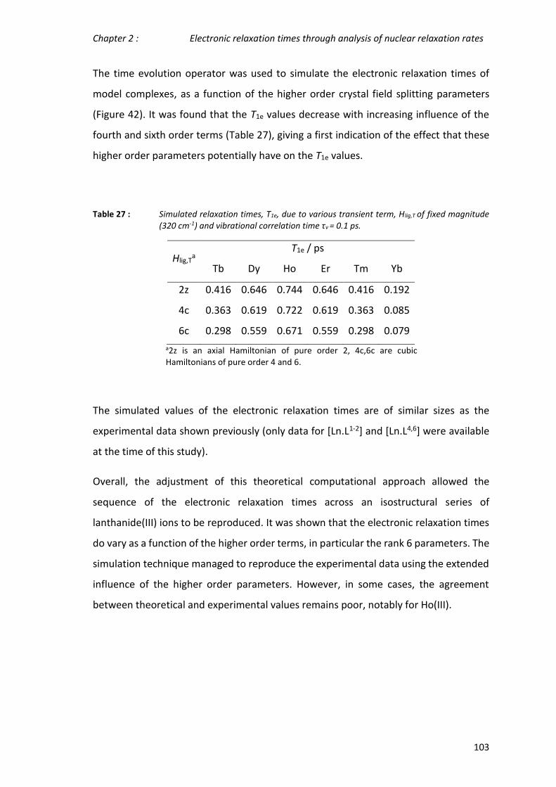
Chapter 2 : Electronic relaxation times through analysis of nuclear relaxation rates
103
The time evolution operator was used to simulate the electronic relaxation times of
model complexes, as a function of the higher order crystal field splitting parameters
(Figure 42). It was found that the T1e values decrease with increasing influence of the
fourth and sixth order terms (Table 27), giving a first indication of the effect that these
higher order parameters potentially have on the T1e values.
Table 27 : Simulated relaxation times, T1e, due to various transient term, Hlig,T of fixed magnitude (320 cm-1) and vibrational correlation time τv = 0.1 ps.
Hlig,Ta
T1e / ps
Tb Dy Ho Er Tm Yb
2z 0.416 0.646 0.744 0.646 0.416 0.192
4c 0.363 0.619 0.722 0.619 0.363 0.085
6c 0.298 0.559 0.671 0.559 0.298 0.079
a2z is an axial Hamiltonian of pure order 2, 4c,6c are cubic Hamiltonians of pure order 4 and 6.
The simulated values of the electronic relaxation times are of similar sizes as the
experimental data shown previously (only data for [Ln.L1-2] and [Ln.L4,6] were available
at the time of this study).
Overall, the adjustment of this theoretical computational approach allowed the
sequence of the electronic relaxation times across an isostructural series of
lanthanide(III) ions to be reproduced. It was shown that the electronic relaxation times
do vary as a function of the higher order terms, in particular the rank 6 parameters. The
simulation technique managed to reproduce the experimental data using the extended
influence of the higher order parameters. However, in some cases, the agreement
between theoretical and experimental values remains poor, notably for Ho(III).

Chapter 2 : Electronic relaxation times through analysis of nuclear relaxation rates
104
2.4 Summary & Conclusions
The estimated electronic relaxation times of the lanthanide(III) ions, generally, follow
the trends first observed by Alsaadi in 1980.66,67 It was found that a change in the
symmetry of the complexes and the different anionic donor groups affect the electronic
relaxation times of the lanthanide(III) ions to different degrees, depending on the
lanthanide(III) ion itself. Especially, complexes Ho(III) and Er(III) were affected by the
changes in the coordination environment.
2.4.1 The impact on ligand design and lanthanide(III) selection
Prior to this thesis, there were only a few literature values available for the electronic
relaxation time of lanthanide(III) ions in solution.20,28,66–68
In the systems presented here, the electronic relaxation time not only has a dominant
effect at low magnetic field strengths, as suggested by simulations and consistent with
the Solomon-Bloembergen Morgan equations (Figure 43), but an effect on the R1 values
at higher magnetic field strengths is also visible. Therefore, even the lanthanide(III) ions
with comparatively low magnetic moments (e.g. Er(III), Tb(III)) possess nuclear
relaxation rates as high as those with higher effective magnetic moments (Tb(III), Dy(III)
and Ho(III)).
Consequently, the consideration of the electronic relaxation times is not only important
for paramagnetic probes to be used at low magnetic field strengths (e.g. contrast and
shift agents for MRI), but, potentially, in probes that are designed to be used at higher
magnetic field strengths (e.g. in protein tagging).53,55,61,84
The extensive datasets presented here enhance our capability to estimate electronic
relaxation times, and also to predict nuclear relaxation times by considering the
coordination environment, its symmetry and their combined impact on the local ligand
field.

Chapter 2 : Electronic relaxation times through analysis of nuclear relaxation rates
105
Figure 43 : Simulation of the dependence of R1 on T1e at a variety of fields (295 K, µeff = 10 BM, r = 6.5 Å, τR = 250 ps).
The selection of lanthanide(III) ions has to be considered more carefully in paramagnetic
probe design. Normally, Dy(III) is considered to provide the ideal relaxation and shift
properties among the non-Gd(III) based agents.23 Depending on the coordination
environment, this thinking has to be revised. By introducing a high symmetry element,
e.g. [Ln.L7] to [Ln.L9]+, the nuclear and electronic relaxation times of Tb(III) and Dy(III)
were significantly increased, while the values for the other lanthanide(III) ions
decreased. However, by changing the anionic donor groups from carboxylate to
phosphinate based systems, the nuclear and electronic relaxation times of Er(III) were
increased the most, while Tb(III) and Dy(III) relaxation times did not vary.
2.4.2 The impact of large crystal field splitting parameters on the total
angular momentum, J
In the axially symmetric lanthanide(III) complexes, the estimated electronic relaxation
times increase as a function of the second order crystal field splitting parameters. It is
proposed herein that the electronic relaxation time is directly influenced by the crystal
field splitting parameters. In highly symmetrical systems, the estimated values of the

Chapter 2 : Electronic relaxation times through analysis of nuclear relaxation rates
106
electronic relaxation times of the lanthanide(III) ions follow the order: [Tb, Dy, Er] > Ho
> [Tm, Yb].
However, in low symmetry systems the order is different, presumably due to the greater
influence of the higher order crystal field splitting parameters. Here, electronic
relaxation times and the nuclear relaxation rates of, for example, the Er(III) and Ho(III)
complexes are influenced more than for the other lanthanide(III) ions. This behaviour
was attributed to the crystal field splitting influencing the individual lanthanide(III) ions
differently. It was not possible to quantify the influence of the higher order parameters,
but the effects of different anionic donor groups was used to show how different ligand
field strengths can influence the electronic relaxation times.
The crystal field in the cyclen-based complexes assessed here, measured in the form of
the 𝐵02 parameters, is relatively large (700 cm-1). It can be assumed that for the low
symmetry system, the higher order parameters contribute significantly more to the
overall crystal field splitting. In addition, the 𝐵02 value estimated here was calculated via
the method developed originally by Binnemans9. However, Binnemans himself revised
his method, proposing that the method underestimates the size of the parameter.10 In
the original proposal, the ΔJ=1 splitting of the Eu(III) emission spectrum was multiplied
by a factor of 3.33. This calculation was later revised with a factor of 4.05, which will
increase all the 𝐵02 by a common factor of 1.2. Therefore, the actual size of the second
order crystal field splitting parameters is not easy to estimate and, therefore, could lie
in between these two factors.
Considering the low symmetry systems, where the higher order parameters can
contribute significantly to the overall crystal field splitting, the size of the ligand field is
of similar magnitude (500 – 1000 cm-1) to the spin orbit coupling. This correspondence
leads to J-mixing of states associated with less well defined electronic energy levels of
the lanthanide(III) ions. It can be safely assumed that the zero field splitting due to the
total angular momentum and the crystal field splitting parameters lead to a complicated
splitting of the energy levels and that this splitting modulates the electronic relaxation
times. J-mixing can also affect the magnetic properties of the lanthanide(III) ions in
terms of the magnetic susceptibility of a given complex. This phenomenon might explain

Chapter 2 : Electronic relaxation times through analysis of nuclear relaxation rates
107
the behaviour of the nuclear relaxation rates at the high field regime. This aspect will be
further discussed in chapter 3 and 4.

Chapter 3 : The discrepancies in Bleaney’s theory of magnetic anisotropy
108
3. The discrepancies in Bleaney’s theory of
magnetic anisotropy

Chapter 3 : The discrepancies in Bleaney’s theory of magnetic anisotropy
109
Bleaney’s theory of magnetic anisotropy was first postulated in 19722 and is still widely
accepted as the most useful description of the theory of magnetic susceptibility
anisotropy for lanthanide(III) complexes. Over the years, many discrepancies in the
original theory have been discussed. Of these, the discussions by Binnemans et al.10,76,77
are most pertinent and relate to the validity of the key assumptions, also to be discussed
herein.
The various isostructural series of lanthanide(III) complexes studied for their relaxation
behaviour in chapter 2 provide a good starting point for an experimental investigation
into the theory of magnetic anisotropy and its effects on the pseudocontact shift in
solution-state NMR spectroscopy.
3.1 Bleaney’s theory of anisotropy
The magnetic susceptibility anisotropy arises from the crystal field splitting of the
ground state J energy levels of the lanthanide(III) ions and the related thermal
population of low lying levels. Bleaney’s theory of magnetic anisotropy is based on the
temperature expansion of the magnetic susceptibility. In axially symmetric systems, the
magnetic susceptibility is different along the three quantization axes (x, y and z), leading
to anisotropic behaviour described by equation (7):
Δ𝜒 = −𝑁𝐴
𝜇𝐵2
20(𝑘𝐵𝑇)2 𝐵0
2(1 + 𝑝)𝐶𝐽 (7)
where Δχ is the change in the magnetic susceptibilities along the directions of Cartesian
coordinates (χx,χy,χz), NA is the Avogadro number, µB is the Bohr magneton, kB is the
Boltzmann constant and 𝐵02 is the second order crystal field splitting parameter. The
term (1+p) corresponds to the thermal population of the lanthanide ion and the CJ is the
Bleaney constant, which is given by equation (3):
𝐶𝐽 = 𝑔𝐽2⟨𝐽‖𝛼‖ 𝐽⟩𝐽(𝐽 + 1)(2𝐽 − 1)(2𝐽 + 3) (3)

Chapter 3 : The discrepancies in Bleaney’s theory of magnetic anisotropy
110
where ⟨𝐽‖𝛼‖ 𝐽⟩ is a numerical coefficient, J is the spin-orbit coupling and gJ is the
electron g-factor. The magnetic anisotropy was, largely, assumed to be independent of
the coordination environment of the lanthanide(III) complex, which would lead to a
specific order of the magnetic anisotropy, among any given series of lanthanide(III)
complexes (Table 28).
Table 28 : Overview of Bleaney constants, and the electronic properties of selected lanthanide(III) ions.2
Ln3+ J ⟨𝐽‖𝛼‖ 𝐽⟩ CJ CJ normaliseda
Tb 6 0.0101 -157.5 -87
Dy 15/2 -0.0076 -181.0 -100
Ho 8 -0.0022 -71.2 -49
Er 15/2 0.0025 58.8 33
Tm 6 0.0101 95.3 53
Yb 7/2 0.0318 39.2 22 aThe normalised values are normally quoted.
3.1.1 Assumptions in Bleaney’s theory and its limitations
In his paper B. Bleaney opens his discussion with the following statement,
“We consider first the magnetic moment of a rare earth ion as arising from its ground J
manifold, whose 2J+1 levels are split by the ligand field by varying amounts which
overall do not exceed kT in energy[…]”85
In wavenumbers, kT corresponds to a size of 205 cm-1 at 295 K. The aqua-complexes
originally investigated by Bleaney have a smaller crystal field splitting (<100 cm-1), but
many lanthanide(III) complexes possess a splitting due to the crystal field of up to
1000 cm-1.12,19,49,78 Therefore this assumption is hardly valid for such lanthanide(III)
complexes.
In addition, it was assumed that the main contribution to the crystal field splitting arises
from the second rank parameters 𝐵02 and 𝐵2
2, in which 𝐵22 is generally found to be much

Chapter 3 : The discrepancies in Bleaney’s theory of magnetic anisotropy
111
smaller than 𝐵02 (e.g. 110 vs 20 cm-1)10,83. However, the higher rank crystal field splitting
parameters can vary significantly in size from 𝐵02 and were completely neglected in
Bleaney’s theory of magnetic anisotropy. Depending on the symmetry of the
lanthanide(III) complex, the higher order parameters (e.g. 𝐵04, 𝐵0
6) can provide a major
contribution to the overall crystal field splitting. Golding et al. attempted to incorporate
higher order parameters into the theory, albeit with limited success.3
Implicitly, Bleaney assumed a point electron at the centre of the paramagnetic
lanthanide(III) ion. The electron cloud of the 4f electrons of the lanthanide(III) ions can
be much better described by a spherical or elliptical model using the spherical
distribution of the 4f orbitals, as simulated by Rinehart and Long when assessing the
behaviour of single-molecule magnets.86
Some of these discrepancies in Bleaney’s theory were first highlighted by Binnemans et
al.10,76,77 A theory of magnetic anisotropy should ideally be able to predict the magnetic
anisotropy of lanthanide(III) complexes in isostructural series, where kT is greater than
the crystal field splitting terms, 𝐵02 and 𝐵2
2.
3.2 Control experiments
A few control experiments were performed first to assess the extent to which variations
in the pseudocontact shift conform to Bleaney’s theory. By varying the temperature and
measuring the pseudocontact shift, it was possible to investigate first the influence of T
on the magnetic anisotropy. If additional terms with higher order parameters were
present, the overall temperature dependence should change, as different power terms
in temperature would be introduced.

Chapter 3 : The discrepancies in Bleaney’s theory of magnetic anisotropy
112
3.2.1 Determining the temperature dependence
The temperature dependence proposed by Bleaney’s theory was 1 / T2 and can easily
be investigated by variable temperature NMR spectroscopy.
Scheme 9 : Structure of [Ln.L4]3+ and labelling scheme of the 1H resonance.
A wide range of complexes was analysed for their temperature dependence. Almost all
complexes were investigated in the range from 298 to 323 K, but only a few examples
are shown (further examples are given in Appendix 3). The behaviour of [Tm.L4]3+ was
analysed over a much wider temperature ranging from 241 to 319 K (Figure 44).

Chapter 3 : The discrepancies in Bleaney’s theory of magnetic anisotropy
113
Figure 44 : Variation of the chemical shift of various resonances of [Tm.L4]3+ with 1 / T2 from 241 to 319 K, (CD3OD, 11. 7 T). A steeper gradient indicates a bigger shift in ppm / K (Hax = 1.32, PhH = 0.16, PhH2 = 0.15, paraH = 0.17, CH3 = 0.11).

Chapter 3 : The discrepancies in Bleaney’s theory of magnetic anisotropy
114
A good correlation between chemical shift data and the inverse temperature squared
was found in all cases. Depending on the polar coordinates of a resonance and,
consequently, the internuclear distance to the paramagnetic centre and the angle to the
principal magnetic axis of the complex, the temperature gradients of the resonances are
different. A steeper gradient leads to a bigger shift per unit temperature (ppm / K).
The axial cyclen ring protons normally have the highest temperature gradient compared
to the other resonances owing to their proximity to the lanthanide(III) ion and the large
(3cos2θ-1) term. A steeper temperature gradient is desirable in probes that are designed
to measure temperature in vivo. Commonly, the CH3 resonance of [Tm.DOTMA]- has
been used to map temperature.47,50 Its temperature gradient of 0.62 ppm / K is not
necessarily the highest observed in the 1H NMR spectrum of [Tm.DOTMA]-, but
combined with its high signal intensity over the other resonances, it constitutes a useful
probe for measuring temperatures in vivo (Appendix 3, SI-Table 87).
The variation of pseudocontact shift with temperature can be complicated as multiple
factors can influence the shifts. The aromatic and the methyl resonances in [Tm.L4]3+ are
clustered in the area of (-11) to (-14) ppm at room temperature. With decreasing
temperatures, however, the proton resonances show slightly different temperature
gradients, which leads to the resonances being in a different order to that observed at
room temperature (Figure 45).

Chapter 3 : The discrepancies in Bleaney’s theory of magnetic anisotropy
115
Figure 45 : Illustration of part of the 1H NMR spectrum of [Tm.L4]3+ at varying temperatures, (CD3OD, 11.7 T). The aromatic and CH3 resonances are shown.
The complex [Ln.L4]3+ possesses time-averaged C4 symmetry and has second order
crystal field splitting parameter (-450 cm-1) of moderate size. The temperature
dependence of the phosphinate systems that were hypothesised to have a significant
contribution from higher order crystal field parameters (see chapter 2) were also
investigated. As an example, the behaviour of [Dy.L8] is presented in Figure 46.

Chapter 3 : The discrepancies in Bleaney’s theory of magnetic anisotropy
116
Figure 46 : Illustration of part of the 1H NMR spectrum showing the tBu resonance of [Dy.L8] at varying temperatures (D2O, 16.5 T). Major (SAP, q=0) and minor (TSAP, q=1) isomers are shown, in the ratio of 4:1 that did not change with temperature.
The higher order parameters should, in theory, provide additional terms with a higher
order T dependence, which may alter the temperature dependence from the predicted
1 / T2 behaviour proposed in Bleaney’s theory. However, no such behaviour was found
and a linear trend was still observed for the chemical shift vs 1 / T2. Previous literature
studies also proved to be inconclusive on this issue.3,76 In addition, McGarvey concluded
for the 1 / T2 term to be the dominant one.62
3.2.2 The contact shift contribution
The observable shift consists of three different contributions. The contact shift, the
diamagnetic shift and the pseudocontact shift.
𝛿𝑜𝑏𝑠𝑣 = 𝛿𝑐𝑜𝑛𝑡𝑎𝑐𝑡 + 𝛿𝑑𝑖𝑎 + 𝛿𝑝𝑠𝑒𝑢𝑑𝑜

Chapter 3 : The discrepancies in Bleaney’s theory of magnetic anisotropy
117
Resonances were measured in comparison to a diamagnetic reference complex, namely
the Y(III) analogue, to allow examination of the diamagnetic contribution to the
observable shift. Additionally, only resonances with an internuclear distance of greater
than 4.5 Å from the paramagnetic lanthanide(III) ion were considered in order to
exclude any possibility of a contact shift contribution, as it is a diminishing contribution
at larger distances.23 However, for nuclei that are directly linked to the lanthanide(III)
ion via a covalent bond, the influence of the contact shift can be quite drastic. The 31P
resonances in [Ln.L2] have an internuclear distance to the lanthanide(III) centre of about
3.7 Å (X-ray, 120 K)29 and are also directly linked to the lanthanide(III) ion via the oxygen
σ-bond. The variation of the observed 31P NMR shift for the [Ln.L2] series is given in Table
29.
Table 29 : Overview of the observed chemical shifts of the 31P resonance of [Ln.L2] (CD3OD, 11.7 T).
Ln3+ δP / ppm ΔδP / ppma CJ <Sz> CJ / <Sz>
Ce 27.8 4.0 -6.3 0.98 6.4
Pr 31.3 7.5 -11 2.97 3.7
Nd 21.0 -2.8 -4.2 4.49 0.9
Sm 31.4 7.6 -0.7 -0.06 11.7
Eu 16.6 -7.2 4 -10.68 0.4
Tb -35.7 -59.5 -87 -31.82 2.7
Dy -15.9 -39.7 -100 -28.55 3.5
Ho -24.6 -48.4 -39 -22.63 1.7
Er -10.5 -34.3 33 -15.37 2.1
Tm 8.4 -15.4 53 -8.21 6.4
Yb 17.7 -6.1 22 -2.54 8.5 aThe change in the observed shift is compared to the Y(III) analogue (+23.8 ppm).
The expectation value <Sz> gives an indication of the strength of the contact shift for a
lanthanide(III). In addition calculating the ratio of the Bleaney constant of the
expectation values allows quantification of the effect of the pseudocontact shift over
the contact shift. A small value will indicate a big influence of the contact shift , if
present. Both Tm(III) and Yb(III) show big values for the ratio indicating a diminishing
effect even when the contact shift is present. However, Eu(III) and Nd(III) would show a
big influence. The similar ratio for Tb(III) and Dy(III) should be noted.

Chapter 3 : The discrepancies in Bleaney’s theory of magnetic anisotropy
118
.
The changes in the shift do not follow the magnitude or even the sign of the Bleaney
constant. The importance of analysing resonances with a sufficiently large internuclear
distance and no direct coordination to the lanthanide(III) ion is emphasised.
3.3 Pseudocontact shift data
Chemical shift data for resonances that are ≥ 4.5 Å from the paramagnetic centre were
analysed to avoid any contact shift contribution, using a wide variety of isostructural
lanthanide(III) complexes. The isostructural series were split into groups, similar to the
classification used in chapter 2. First, the three C3-symmetric complex that possess a
small crystal field splitting series were analysed ([Ln.L1-3]). The study was then extended
to other highly symmetric complex series, e.g. [Ln.L4]3+.
Due to the peculiar relaxation behaviour of the phosphinate complexes ([Ln.L2,5,6,8,11]),
they were analysed separately. Finally, the complexes containing the tBu reporter group
([Ln.L7-9]) and related derivatives will be discussed to allow further insight into
perturbations created by varying ligand fields.
In theory, the magnitude of the measured second order crystal field splitting parameter,
𝐵02, can give an indication as to how closely these systems may follow the pseudocontact
shifts predicted by Bleaney’s theory (Table 30), assuming that 𝐵02 > 𝐵2
2.

Chapter 3 : The discrepancies in Bleaney’s theory of magnetic anisotropy
119
Table 30 : Overview of the isostructural series [Ln.Lx] by the analysis of the estimated second order
crystal field splitting parameters, 𝑩𝟎𝟐 (derived from the ΔJ = 1 splitting of Eu(III) emission
spectrum), 295 K.
[Ln.Lx] 𝐵02 / cm-1 a
[Ln.L1] +75
[Ln.L2] +110
[Ln.L3]3+ +235
[Ln.L4]3+ -470
[Ln.L5]- -700
[Ln.L6] -550
[Ln.L7] -455
[Ln.L8] -570
[Ln.L9]+ -355 aAssociated error in the estimation of 𝐵0
2 is ±40 cm-1.
3.3.1 The C3 symmetric series of complexes
The three complexes ([Ln.L1-3]) differ in the constitution of the oxygen donor. The ligand
field in these three 9N3 systems is comparatively small and is less than ([Ln.L1-2]) or of
the same order as kT ([Ln.L3]3+). Due to the Cn symmetry of these three systems, the
second order crystal field splitting parameter, 𝐵02, should characterise the overall crystal
field splitting of each complex. Bearing this in mind, it was expected that the
pseudocontact shifts of these three complexes would follow Bleaney’s theory relatively
well.

Chapter 3 : The discrepancies in Bleaney’s theory of magnetic anisotropy
120
Scheme 10 : Structures of the three C3 symmetric, 9N3 based complex series [Ln.L1-3] with assignment of the pyridyl resonances.
The imposed distance constraint (r ≥ 4.5 Å) and the compact nature of the 9N3
complexes limits the analysis of the pseudocontact shift to the common pyridyl
resonance (labelled pyH3, pyH4 pyH5).
Of course, a correct NMR assignment of the ligand resonances is of utmost importance
in this analysis. Due to the discrepancies in the theory, it was not regarded as sufficient
to assign the ligand resonances of the complexes based on trends in chemical shift data
alone. However, the relaxation rates and their dependence on the internuclear distance,
r, allow accurate mapping of the lanthanide(III) complexes. In the fitting procedure
presented, the estimated internuclear distances together with the availability of the X-
ray structures allow a full and self-consistent assignment of the 1H NMR resonances in
each complex (Table 31).

Chapter 3 : The discrepancies in Bleaney’s theory of magnetic anisotropy
121
Table 31 : Overview of the chemical shift of the pyridyl resonance (pyH3,4,5) of [Ln.L1-3] with estimated average internuclear distances through single fitting analysis (295 K, [Ln.L1] in D2O, [Ln.L2,3] in CD3OD) and X-ray structural analysis (120 K).
1H
δH / ppm
pyH3 pyH4 pyH5
[Ln.L1] [Ln.L2] [Ln.L3]3+ [Ln.L1] [Ln.L2] [Ln.L3]3+ [Ln.L1] [Ln.L2] [Ln.L3]3+
Tb 0.1 -7.1 -11 4.9 -2.3 -3.2 4.1 -1.3 -4.4
Dy 9.4 -1.4 1.9 10.6 1.4 5.0 11.0 2.7 3.0
Ho 3.9 2.3 -5.5 6.2 4.1 -0.4 6.5 5.5 0.5
Er 8.3 13.6 8.2 7.9 11.9 7.9 6.3 12.6 8.2
Tm 14.2 18.6 23 13.5 16.4 19.6 14.2 17.8 19.2
Yb 9.5 10.7 11.6 9.1 10.3 11.2 8.8 10.7 11.4
Average
r /Åa 5.56 5.71 5.50 6.28 6.58 6.46 5.72 5.66 5.50
X-ray r /
Åc 5.40 5.53 5.48 6.22 6.36 6.26 5.50 5.59 5.45
𝐵02 /
cm-1 b 75 110 235
aAverage over all 6 lanthanide(III) ions examined. bRespective errors of around 40 cm-1. cX-ray data taken from [29,74,80]
According to Bleaney’s theory the variation of the pseudocontact shift should be
proportional to the second order crystal field splitting parameter. The illustration in
Figure 47 shows the behaviour of the pyH3 resonance of each lanthanide(III) complex of
the three series with increasing 𝐵02.

Chapter 3 : The discrepancies in Bleaney’s theory of magnetic anisotropy
122
Figure 47 : Illustration of the pyH3 resonances of the series of [Ln.L1-3], taken from NMR data (295
K, 9.4 T, [Ln.L1] in D2O, [Ln.L2,3] in CD3OD). Sizes of 𝑩𝟎𝟐 are highlighted. CJ values follow
Tb(-89) , Dy(-100), Ho(-49), Er(+33) , Tm(+55), Yb(+22).
A general increase of the pseudocontact shit is evident from [Ln.L1] to [Ln.L3]3+ with
increasing 𝐵02. However, the order and strengths of the magnetic anisotropies of some
lanthanide(III) ions show irregularities. In particular, Er(III) stands out due to the almost
total absence of a pseudocontact shift in both [Er.L1] and [Er.L3]3+. The complex [Dy.L1]
also shows unexpected behaviour due to the variable sign of the shift change. This is the
only case observed where the sign of a pseudocontact shift value does not follow the
trend of the sign of the Bleaney constant.
The chemical shifts of the pyH3 resonance do not follow the predicted values of the
magnetic anisotropy. The expected order of Dy(III) > Tb(III) >> Ho(III) is not maintained
in each series. The Tb(III) complexes always give rise to the biggest pseudocontact shift
and every Dy(III) complex behaves in an anomalous way. It is surprising that even in
these systems with a small ligand field, the order of magnetic anisotropy predicted by

Chapter 3 : The discrepancies in Bleaney’s theory of magnetic anisotropy
123
Bleaney’s theory is not followed. The shift behaviour of pyH4 and pyH5 in these
complexes behave similarly (selected 1H NMR and data in Appendix 3).
To investigate the extent to which the pseudocontact shifts differ from the expected
strengths of the magnetic anisotropy from the Bleaney constant, CJ, the two parameters
were plotted against each other. A linear relationship was added as a visual aid, which
assumes ideal behaviour for the Yb(III) analogues and extrapolates the predicted shift
from the Yb(III) analogues projects. The Yb(III) analogue was selected because it has the
lowest magnetic susceptibility and is generally assumed to be the lanthanide(III) ion
whose behaviour can be predicted most accurately in terms of shift and
relaxation.19,87,88

Chapter 3 : The discrepancies in Bleaney’s theory of magnetic anisotropy
124
Figure 48 : Correlation of the pseudocontact shift data of the pyH3 resonance of [Ln.L1,2,3] with the Bleaney constant, CJ (295 K, 9.4 T, [Ln.L2,3] in CD3OD, [Ln.L1] in D2O).

Chapter 3 : The discrepancies in Bleaney’s theory of magnetic anisotropy
125
Figure 48 illustrates the behaviour of the chemical shift anisotropy of each
lanthanide(III) ion in the three 9N3 systems. Data for the pyH3 resonances are shown
here, but similar analyses were performed for the pyH4 and pyH5 resonances (Appendix
3, SI-Figure 3 - 9), and gave rise to the same sort of plot.
As indicated by Figure 47, the sizes of the magnetic anisotropy hardly follow the sizes
and sequence for the lanthanide(III) ions predicted by Bleaney’s theory. If the theory is
followed, a linear trend should be observed between the pseudocontact shift and the
Bleaney constant.
Notwithstanding the sign of the Bleaney constant, the sequence for the strength of the
magnetic anisotropy and therefore the pseudocontact shift should follow the order:
Dy > Tb >> Tm > Ho >> Er > Yb. This sequence is not conserved at all within these three
systems. In every cases, the Tb(III) systems possess the largest magnetic anisotropy,
while Tm(III) and Dy(III) have a similar size of shift followed by Ho(III) and Yb(III). The
behaviour of the Er(III) analogues is curious in both [Ln.L1] and [Ln.L3]3+, as there is little
or no apparent pseudocontact shift.
The pyridine ring is directly coordinated to the lanthanide(III) ion. This could indicate a
contribution of the contact shift to the overall observable shift of the pyridyl
resonances. However, as it was indicated in Table 29, both Tb(III) and Dy(III) have similar
ratios of CJ / <Sz>, which would indicate a similar overall shift behaviour. This is not
observed in the data present here.
The discrepancies in Bleaney’s theory were highlighted earlier and it was expected that
in these low ligand field systems the experimental data should be relatively well
behaved with respect to the theory. It was found that even in these systems the theory
fails to describe the magnetic anisotropy in terms of magnitude, although, the sign of
the shift is correctly predicted in all cases with the exception of [Dy.L1]. However, a
general increase of the overall pseudocontact shifts can be observed with increasing 𝐵02.
A linear variation was not observed, indicating that additional terms are required in
order to describe the pseudocontact shift.

Chapter 3 : The discrepancies in Bleaney’s theory of magnetic anisotropy
126
3.3.2 The C4 symmetric complexes
The tetra-amide complex series [Ln.L4]3+ has multiple resonances with an internuclear
distance to the paramagnetic centre of ≥ 4.5 Å, allowing consideration of the observable
shift without a contact shift contribution.
Scheme 11 : Structure of the tetra-amide complex S-[Ln.L4]3+.
Among the isostructural series studied here, the [Ln.L4]3+ series possess an average
strength crystal field splitting (-470 cm-1). Similar to [Ln.L1-3], it can be assumed that the
higher order 𝐵𝑞𝑘 parameters do not play a significant role due to high symmetry. The
plots of the pseudocontact shifts of individual resonances against the Bleaney constant
of the [Ln.L4]3+ series (Figure 49) show a reasonably good agreement with the theory.

Chapter 3 : The discrepancies in Bleaney’s theory of magnetic anisotropy
127
Figure 49 : Correlation of the pseudocontact shift of the CH3 (top left), PhH (top right), PhH2 (bottom left) and paraH (bottom right) against the Bleaney constant, CJ (295 K, 9.4 T, D2O).

Chapter 3 : The discrepancies in Bleaney’s theory of magnetic anisotropy
128
With the exception of the phenyl ring paraH resonance, every pseudocontact shift
measured follows the sequence and magnitude predicted by Bleaney’s theory relatively
closely. The deviation from the fitted line is relatively small compared to the 9N3 series
of complexes. Overall, the magnetic anisotropy is described relatively well.
The estimated second order crystal field splitting parameter, 𝐵02, is roughly twice the
size of the value that Bleaney estimated as a maximum in his theory (470 vs
215 cm-1). However, it seems the theory describes the [Ln.L4]3+ series much more
accurately than the 9N3 systems [Ln.L1-3], notwithstanding the bigger crystal field
splitting.
In the [Ln.DOTMA]- series, there are two major isomers in solution, whose relative
proportion and hydration number changes as the size of the lanthanide(III) ion
decreases across the lanthanide series. Thus, the Eu(III) and Tb(III) form a 9 coordinate,
q = 1 complex in aqueous solution with a monocapped twisted square antiprismatic
structure (TSAP) and square-antiprismatic (SAP) isomers. As the size of the
lanthanide(III) ion decreases, the major (TSAP) isomer becomes 8-coordinate (q = 0).
However, the minor isomer does not change hydration number across the series and
was therefore analysed here.49 The Yb(III) analogue does not form this isomer, but
[Eu.DOTMA] was analysed instead.
Figure 50 : Correlation of the pseudocontact shift of the minor isomer (SAP, q=1) of the CH3 resonance of R,S - [Ln.DOTMA]- against the Bleaney constant, CJ (295 K, 9.4 T, D2O).89

Chapter 3 : The discrepancies in Bleaney’s theory of magnetic anisotropy
129
The second order crystal field splitting parameter of [Ln.DOTMA]- is one of the biggest
observed (-700 cm-1, major isomer). The pseudocontact shifts of [Ln.DOTMA]- do not
follow the expected trend (Figure 50). A linear correlation could be made between
Eu(III), Er(III) and Tb(III), but Ho(III) and especially Tm(III) show much larger
pseudocontact shifts.
The Tm(III) and Yb(III) analogues also share a common major isomer (TSAP, q=0). Their
respective pseudocontact shifts (102.8 and 13.5) differ by a factor of > 7 (more than 100
ppm). Such a shift variation does not correlate with their normalised CJ values of +53
and +22.
3.3.3 Phosphinate complexes
The tetra-methylphosphinate complex series [Ln.L5]- also possess time average C4
symmetry and normally might be analysed together with the other highly symmetrical
complexes. However, as pointed out in the chapter 2, section 2.2.3.2, it is more
appropriate to analyse the various phosphinate complex series as a group, as they are
each octadentate (q = 0) systems, lacking the axial water found in [Ln.L4]3+, and in the
minor isomer of [Ln.DOTMA]-.
Scheme 12 : Structures of the 8-coordinate phosphinate based complexes: [Ln.L5,6,8]
The pseudocontact shift data for these complexes is summarised in Figure 51.

Chapter 3 : The discrepancies in Bleaney’s theory of magnetic anisotropy
130
Figure 51 : Variation of the pseudocontact shift of [Ln.L5]- (CH3), [Ln.L6] (CF3) and [Ln.L8] of the tBu resonances against the Bleaney constant, CJ (295 K, 9.4 T, D2O).

Chapter 3 : The discrepancies in Bleaney’s theory of magnetic anisotropy
131
The pseudocontact shifts for these systems do not correlate well with the Bleaney
constant, CJ, in each of the phosphinate complexes, including the [Ln.L2] resonances
shown earlier. In particular, the Tm(III) complexes show larger shifts than predicted. The
Tb(III) and Dy(III) complexes possess similar shifts. The expected linear trend is not
followed. Additionally, the Ho(III) and Er(III) analogues seem to have switched order in
terms of the size of the magnetic anisotropy.
Out of all the phosphinate based systems, the [Ln.L6] complex series follows the theory
most faithfully, exemplified by looking at the P-CH3 resonance (Figure 52), but the
characteristic switch of the order for Ho(III) and Er(III) is still present.
Figure 52 : Correlation of the pseudocontact shift of the CH3 resonance for [Ln.L6] against the Bleaney constant, CJ (295 K, 9.4 T, D2O).
The 1H NMR shift of the PCH3 resonances of [Ln.L5]- is less shifted than the mean P-CH3
resonance shifts in the other low symmetry complexes (e.g. [Tm.L5]- = -27.2,
[Tm.L6] = -52.8, [Ln.L11] = -55.4 Appendix 3, SI-Table 78 -85). Even though the [Ln.L5]-
series possesses one of the highest crystal field splitting parameters (-700 cm-1), it can
be assumed that due to the low symmetry in the other complexes, their higher order
crystal field splitting parameters may be larger and could contribute more to the overall
crystal field splitting, leading to a bigger overall shift than for [Ln.L5]-.

Chapter 3 : The discrepancies in Bleaney’s theory of magnetic anisotropy
132
Overall, these phosphinate systems, do not follow the sequence and magnitudes of the
expected pseudocontact shifts according to Bleaney’s theory of magnetic anisotropy.
Similar observations can be made for [Ln.L11] (Appendix 3, SI-Figure 11 and SI-Table 85).
3.3.4 Analysis of tBu resonances in related pyridyl complexes
The tBu reporter group is useful for 1H NMR studies, as the three methyl groups are
homotopic and isochronous.46 A wide range of derivatives of complexes was available
to analyse. In each case, relaxation analysis had established that the tBu-Ln(III)
distance was 6.6 ±0.2 Å.
Scheme 13 : Structures of the complexes [Ln.L7-9].
The structural similarities allow a direct comparison of the shift behaviour of the tBu
resonance. The second order crystal field splitting parameters of [Ln.L7-8] were
estimated to be in a similar range (-550 and -570 cm-1 respectively), while the estimated
parameter for [Ln.L9]+ is somewhat small (355 cm-1). The splitting of the ΔJ = 1 band of
[Eu.L7S] is the same as [Eu.L7]. An illustration of part of the 1H NMR spectra for selected
Dy(III) complexes is given in Figure 53.

Chapter 3 : The discrepancies in Bleaney’s theory of magnetic anisotropy
133
Figure 53 : Illustration of part of the 1H NMR spectrum of [Ln.L7], [Ln.L8] and [Ln.L8CO2], (295 K 9.4 T, D2O). Major (SAP) and minor isomer (TSAP) of the tBu resonance highlighted. No values
of 𝐵02 was estimated for [Ln.L8CO2]. The changes in hydration number should be noted.
The behaviour of these complexes is exceptional. From [Dy.L7] to [Dy.L8] the tBu shift
changes by almost 60 ppm, even though the splitting of the Eu(III) emission spectrum is
roughly the same. The introduction of the 4-carboamide group further enhances the
shift of [Dy.L8CO] compared to [Dy.L8]. This can be attributed to the effect the different
distribution of the electron density of the pyridine ring has on the ligand field. The py-
Dy(III) interaction is perturbed by the ligand field and changes the observable shift
slightly. The large changes in the observable shift of carboxylates and phosphinates are
too extreme to be able to correlate them with the changes in the splitting due to 𝐵02,
derived from the Eu(III) optical spectral analysis.
A full overview of the shift data of the complexes containing the tBu reporter group is
given in Table 32. The much bigger shift of the 8-coordinate phosphinate complexes can
be observed across the whole series.

Chapter 3 : The discrepancies in Bleaney’s theory of magnetic anisotropy
134
Table 32 : Chemical shift data of the tBu resonance of [Ln.L7,7S,8,9] and the Bleaney constant, CJ, for comparison (295 K, 9.4 T, D2O).
Ln3+ δH / ppma
CJ [Ln.L7] [Ln.L7S]b [Ln.L8] [Ln.L9]+
Tb -11.6 -55.8 -76.9 -7.2 -89
Dy -20.5 -58.9 -75.0 -17.8 -100
Ho -7.4 -26.3 -31.8 -7.0 -49
Er 7.0 x 38.2 3.4 33
Tm 10.8 44.3 67.0 6.2 55
Yb 6.3 x 16.3 9.1 22
ppm / K 0.1 0.3 0.4 0.1
𝐵02 / cm-1 -550 -550 -570 -350
aMajor isomer shown here, minor isomer data available in Appendix 3, SI-Table 82 bMeasured at pD = 8.
The measured temperature gradient follows the strength of the pseudocontact shift; a
larger gradient was observed for the more shifted resonances.
Comparing [Ln.L7] and [Ln.L7S], the shifts are quite different, even though they possess
the same splitting of ΔJ = 1 band in the Eu(III) emission spectrum. The pseudocontact
shifts for the tBu resonance in [Ln.L9]+ are relatively small, when compared to [Ln.L7].
Such behaviour is most likely linked to the ligand field changes, as a neutral pyridyl
donor replaces a carboxylate oxygen and the 𝐵02 values of -550 and -350 cm-1 are
consistent with this interpretation. The Er(III) analogue is hardly shifted, similar to
observation made in [Er.L1,3]. In this complex, the Yb(III) analogue also shows surprising
behaviour. Its observed shift is not only larger than the Er(III) and Tm(III) analogues of
[Ln.L9]+, but also [Yb.L7]. Overall the shift behaviour of [Yb.L9]+ is highly irregular, and
represents the only case where an Yb(III) complex behaves in such a way.
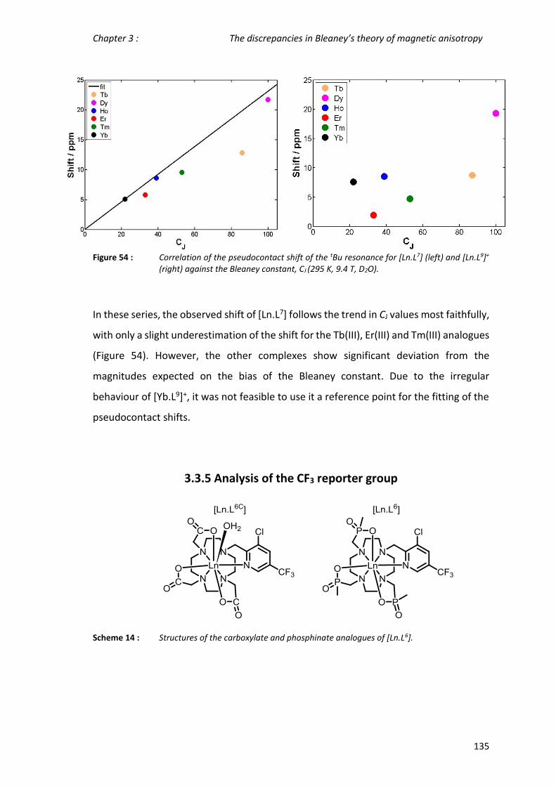
Chapter 3 : The discrepancies in Bleaney’s theory of magnetic anisotropy
135
Figure 54 : Correlation of the pseudocontact shift of the tBu resonance for [Ln.L7] (left) and [Ln.L9]+ (right) against the Bleaney constant, CJ (295 K, 9.4 T, D2O).
In these series, the observed shift of [Ln.L7] follows the trend in CJ values most faithfully,
with only a slight underestimation of the shift for the Tb(III), Er(III) and Tm(III) analogues
(Figure 54). However, the other complexes show significant deviation from the
magnitudes expected on the bias of the Bleaney constant. Due to the irregular
behaviour of [Yb.L9]+, it was not feasible to use it a reference point for the fitting of the
pseudocontact shifts.
3.3.5 Analysis of the CF3 reporter group
Scheme 14 : Structures of the carboxylate and phosphinate analogues of [Ln.L6].

Chapter 3 : The discrepancies in Bleaney’s theory of magnetic anisotropy
136
The 19F shift behaviour of the CF3 resonance in [Ln.L6] was compared to the carboxylate
analogue of the complex ([Ln.L6C]). The large shift differences observed between [Ln.L7]
and [Ln.L8] were also observed in [Ln.L6] (δF = -162.4 ppm) and [Ln.L6C] (δF = -115.1 ppm).
The very large shift difference between analogous carboxylate and phosphinate
complexes is evident and cannot be rationalised easily. It can be postulated that
differences in oxygen polarizability and the change in coordination number, have a
major effect on the overall crystal field splitting. Yet, a more fundamental
reconsideration may be required to rationalise the dramatic differences in shift
behaviour.
3.5 Summary & Conclusions
There are a number of assumptions in Bleaney’s theory of magnetic anisotropy that
could easily be held responsible for the significant differences between the
experimental and theoretical NMR shift data shown here. The main assumptions involve
the crystal field splitting parameters and their influence on the J energy levels. The
original underestimation of the second order crystal field splitting parameters
(𝐵02 << 205 cm-1) and the exclusion of the higher order parameters (e.g. 𝐵0
4, 𝐵06) could
be one of the causes for the big deviations observed.
The overall correlation between the shift range and the 𝐵02 in the axially symmetric
systems is given below (Figure 55). But, even here, the linear dependence, as suggested
by Bleaney, is not limited (R2 ≈ 0.85). Both Tm(III) and Yb(III) analogues behave similarly.

Chapter 3 : The discrepancies in Bleaney’s theory of magnetic anisotropy
137
Figure 55 : Correlation of the total 1H NMR shift range of the Tm(III) and Yb(III) analogues of the axially symmetric systems [Ln.L1-5,9], [Ln.DOTMA]- and [Ln.gDOTA]5- (295 K, 9.4 T, [Ln.L2,3] in CD3OD]) with the second order crystal field splitting parameter, 𝐵0
2, measured for the Eu(III) analogue.
For those complexes possessing a 𝐵02 value of 700 cm-1 ([Ln.L5]-, [Ln.DOTMA] and
[Ln.gDOTA]5-) differences in the spectral behaviour are possibly due to the influence of
the higher order parameters. These parameters should not be neglected in any theory
that describes the pseudocontact shift. Such a contribution was also suggested earlier
by Golding3.
Binnemans76,77 also suggested that the local magnetic anisotropy is modulated by the
shape and degree of distortion of the coordination polyhedron in a series of
lanthanide(III) complexes. An analysis of the twist angle of the mean plane of the 9N3
ring with reference to the three oxygen donor atoms in the X-ray structures of the C3
symmetric complexes ([Ln.L1-3]) was undertaken. There was no correlation between the
twist angles (22 ± 2° in all each system) and the measured magnetic anisotropy (Figure
56), showing that polyhedral distortion does not explain the observed shift variation.74
R² = 0.83
R² = 0.74
0
100
200
300
400
500
600
700
800
0 100 200 300 400 500 600 700 800
Δδ
H/
pp
m
/ cm-1
Tm
Yb
𝐵02

Chapter 3 : The discrepancies in Bleaney’s theory of magnetic anisotropy
138
Figure 56: Views of the X-ray structures of the two diasteroisomers of [Eu.L3]3+: S-Δ-(λλλ) (left) and R-Λ-( δδδ) right (120 K). highlighted the measured twist angles of the O and N planes. No difference in twist angles between Eu(III) and Yb(III) structures was observed. Taken from [74].
The final assumption made by Bleaney concerns the electron distribution. The point-
dipole approximation does not represent the overall electron cloud very well, in
particular in these anisotropic lanthanide(III) complexes. Rinehart and Long86 simulated
the quadrupole moment of the 4f electron cloud using the angular dependence of the
4f orbitals whilst investigating the single molecule magnet behaviour of lanthanide(III)
ions (Figure 57).
Figure 57 : Simulations of the shape of the 4f orbitals (left) and quadrupole approximations of the 4f electron cloud for lanthanide(III) ions (right), based on the total angular momentum, J, the Stevens coefficient and the 4f orbital radius. Taken from [86].
The electron density varies from oblate (in Tb(III), Dy(III), and Ho(III) ions) to prolate
(Er(III), Tm(III) and Yb(III)) explaining the signs of the magnetic anisotropy, as predicted
by Bleaney. The Er(III) case stands out as rather curious as it almost possesses an
isotropic electron distribution, which could explain the lack of pseudocontact shift in
many of the Er(III) analogues analysed here.

Chapter 3 : The discrepancies in Bleaney’s theory of magnetic anisotropy
139
Sessoli et al.90 have recently measured and calculated the position of the easy (principal)
axis of magnetisation in the C4 symmetric [Ln.DOTA]- series. The easy axis of
magnetisation is the energetically favoured direction of the spontaneous
magnetisations and is considered to be parallel to the direction of the C4- symmetry axis
(along axially bound water) in Bleaney’s theory. Their calculations showed that the easy
axis of magnetisation changes steadily from the equatorial plane (90° to axial donor,
H2O) to the axial plane (along axial donor group) from Tb(III) to Yb(III) (Figure 58). Such
behaviour would indicate that the cone of highest anisotropy is not always along the
direction of the axial donor molecule, but will change across the series, according to the
electron density of the ligand. However, an irregularity was found for Er(III), as their
experimental data deviated significantly from the simulation.
Figure 58 : Experimental (angle-resolved magnetometry,pink) and calculated (quantum chemistry simulation, blue) easy axis of magnetisation across the series of [Ln.DOTA]- viewed perpendicular (top) and parallel (bottom) to the four-fold symmetry axis (2 K). Taken from [90].
Due to the changes in the position of the axis of magnetisation the magnetic anisotropy
might be much more complex than anticipated by Bleaney, as the angular reference
point in the (3cos2θ-1) term changes from one lanthanide(III) ion to another
(Figure 58).90,91
Most of the investigations concerning these phenomena originate from studies
optimising the single-molecule magnet behaviour of the lanthanide(III) ions, which
favours a small energy gap between the electronic energy levels. Sessoli and Long both

Chapter 3 : The discrepancies in Bleaney’s theory of magnetic anisotropy
140
concluded that a minimum energy gap (for optimum SMM behaviour) is achieved for
oblate ions when the ligand electron density is focused equatorially, while for prolate
ions, axial ligand electron density is favoured. This effect could be rationalised to
determine the differences in the crystal field splitting across a series of lanthanide(III)
ions, as the paramagnetic electron clouds all interact differently with the ligand electron
density.91
Following this consideration, a maximum energy gap between the J-sub levels is
observed in systems with high crystal field splitting ([Ln.L4-11)]. Therefore prolate ions
(Er, Tm, Yb) may be expected to have the highest magnetic anisotropy in ligand systems
possessing equatorial electron density.86 This is the case for complex systems that have
a hydration value of 0, as there is no contribution from the axial donor group. It is,
indeed, these q = 0 systems, for which the biggest deviations are found with prolate
ions. For example, with Tm(III) systems, where very high pseudocontact shifts were
observed in the phosphinate based complexes and also in q = 0 isomer of
[Tm.DOTMA]-. It is suggested that the magnetic anisotropy in the prolate ions (Er, Tm,
Yb) is much more dependent on the ligand field in these cases, compared to their oblate
counterparts (Tb, Dy, Ho).
In combination with the change in the easy axis of magnetisation across the
lanthanide(III) series, this effect could help to rationalise the pseudocontact shift
behaviour of lanthanide(III) complexes.
On a final note, the size of the crystal field splitting parameters can be of similar
magnitude to the spin-orbit coupling term, which will lead to an effect called J-
mixing.77,92 The uncertainty about the splitting of the energy levels is increased and J
cannot be assumed to be a “good” quantum number anymore. The magnitude of the
Bleaney constant, CJ, is directly connected to these J terms and energy levels. If the
values differ from the theory, the actual Bleaney constant will deviate significantly. Such
behaviour could, at least in part, explain the behaviour of the low symmetry complexes
that possess an overall crystal field energy (-700 cm-1 in 𝐵02, higher in 𝐵0
4 and 𝐵06) of
similar size to the spin orbit coupling (1000 – 2000 cm-1 from Eu(III) to Yb(III)).

Chapter 3 : The discrepancies in Bleaney’s theory of magnetic anisotropy
141
In conclusion, it seems that Bleaney theory has outlived its usefulness and the
limitations highlighted in this work suggest that a better theory of magnetic anisotropy
is required that is more firmly based on the effect of the local ligand, the symmetry and
the relative position of the easy axis of magnetisation.

Chapter 4 : The effect of J-mixing on the magnetic susceptibility
142
4. The effect of J-mixing on the magnetic
susceptibility

Chapter 4 : The effect of J-mixing on the magnetic susceptibility
143
In lanthanide electronic structure theory, the contribution of the spin-orbit coupling to
the splitting of the electronic energy levels has generally been assumed to be much
larger than splitting due to the ligand field. The ligand field and its associated crystal
field splitting has been assumed to be an order of magnitude smaller than the spin-orbit
coupling term and is largely neglected when considering the overall splitting of the
electronic energy levels of the lanthanide(III) ions (Figure 2).2,10
It was made apparent in the previous chapters that the crystal field spitting parameters
can vary significantly for each complex series. Several second order crystal field splitting
parameters, 𝐵02, have been estimated by analysis of the splitting of the ΔJ = 1 band in
the Eu(III) emission spectrum using the method postulated by Binnemans et al9. These
values range from 75 – 700 cm-1, but larger values (up to 1000 cm-1) have been reported
in the literature.10 The size of the crystal field splitting changes across a series of
lanthanide(III) ions due to their different electron clouds and their differing interactions
with the ligand field.10,86 Only the second-order parameter, 𝐵02, is readily obtained by
direct analysis of the Eu(III) emission spectrum. However, depending on the symmetry
of the complex, more parameters will contribute to the overall crystal field splitting. In
particular, for the low symmetry systems, it is presumed that the higher order
parameters have a much more significant contribution.10
The 𝐵02 terms estimated in this thesis were determined using the method developed
originally by Binnemans9. However, Binnemans has revised his analysis, stating that the
method underestimates the size of the parameter.10 In the original proposal, the
splitting of the two transitions in the ΔJ = 1 manifold in the Eu(III) emission spectrum
was multiplied by a factor of 3.33. This was later revised with a factor of 4.05, which will
increase all the 𝐵02 terms by a common factor of 1.2. Therefore, the actual size of the
second order crystal field splitting parameters might be systematically underestimated
in all of the estimations given here and could lie in between the two values. A good
agreement was found in the solid-state between 𝐵02 values derived by iterative spectral
analysis and the separation of the main two bands in the ΔJ = 1 region (585 – 605 nm)
(Figure 59).

Chapter 4 : The effect of J-mixing on the magnetic susceptibility
144
Figure 59 : Correlation of the splitting of the ΔJ =1 band of the Eu(III) emission spectrum of different lanthanide(III) compounds and complexes in the solid-state with the second order crystal field splitting parameter 𝐵0
2. It was proposed that the splitting corresponds to 4.05 times 𝐵0
2.Taken from [10].
4.1 The occurrence of J-mixing
In the most frequently used theories of lanthanide magnetism, it is assumed that the
magnetic susceptibility is independent of the coordination environment of the
lanthanide(III) complexes. Such an assumption requires that the size of the crystal field
splitting is almost an order of magnitude smaller than the spin orbit coupling.10,93
In the systems investigated here, the estimated values of 𝐵02 alone are, in some cases,
almost of the same order of magnitude as the spin-orbit coupling. A large crystal field
splitting results in more overlap between the energy levels split by the total angular
momentum, J, leading to less defined energy levels for the lanthanide(III) ions. This
concept has been reported before.92 Generally, it is assumed that complexes of low
symmetry are more prone to J-mixing.10,92 Experimentally, this effect can lead to
changes in the relative intensities of the various ΔJ = n bands (n = 0 – 4) in , for example,
the Eu(III) emission spectrum.94–96
For the case of J-mixing, the total spin orbit coupling, J, is not considered to be a ‘good’
quantum number anymore. A variety of properties are directly linked to the electronic

Chapter 4 : The effect of J-mixing on the magnetic susceptibility
145
energy levels of the lanthanide(III) ions and their respective J values. In both chapters 2
and 3 of this thesis, the effect of the crystal field splitting on paramagnetic relaxation
and the magnetic susceptibility anisotropy was highlighted.
The magnetic susceptibility anisotropy showed great variation with the crystal field
splitting and it can be postulated that the overall magnetic susceptibility could also be
affected due to its dependence on J. In classical lanthanide magnetism theory, as
originally proposed by Landé97, the effective magnetic moment, µeff is defined as:
𝜇𝑒𝑓𝑓 = 𝑔𝐽 √𝐽(𝐽 + 1) (8)
𝑔𝐽 = 𝐽(𝐽 + 1) + 𝑆(𝑆 + 1) − 𝐿(𝐿 + 1)
2𝐽(𝐽 + 1) (9)
where gJ is the Landé factor (defined in equation 9), S is spin-spin coupling, L is the orbit-
orbit coupling, and J is the total angular momentum or spin-orbit coupling. According to
these theories the values of the magnetic susceptibility will change on consideration of
J-mixing and may be expected to deviate from the ‘free-ion’ values.92,93,97
4.2 Ways of estimating the effective magnetic moments of
lanthanide(III) ions
Three different methods were used to investigate the influence of the coordination
environment on the magnetic susceptibility: firstly, fitting of nuclear relaxation data
(section 4.2.1); secondly, NMR investigations using the bulk magnetic susceptibility shift
(section 4.2.2), lastly measurements in the solid-state using a SQUID magnetometer
(section 4.2.3). The fitted data of the nuclear relaxation rates provides the biggest data
set available, while the other two methods were employed for only a few selected
complexes.

Chapter 4 : The effect of J-mixing on the magnetic susceptibility
146
4.2.1 Fitting of nuclear relaxation data
Measuring the nuclear relaxation rates, R1, at different magnetic field strengths allows
the estimation of the effective magnetic moments of the lanthanide(III) ions, amongst
other parameters, through the fitting of the data to equation 4. The method was
explained in detail in chapter 2.
𝑅1 =2
15 (
µ0
4π)
2
γN
2 𝑔𝐿𝑛2 µ𝐵
2 𝐽 (𝐽 + 1)
𝑟6 [3
𝑇1𝑒
1 + 𝜔𝑁2 𝑇1𝑒
2 + 7𝑇2𝑒
1 + 𝜔𝑒2 𝑇2𝑒
2 ]
+2
5(
μ0
4π)
2 𝜔𝑁2 µ𝑒𝑓𝑓
4
(3kB𝑇)2 𝑟6[3
𝜏𝑟
1 + 𝜔𝑁2 𝜏𝑟
2] (4)
A fixed internuclear distance, r, was used to calculate the effective magnetic moments
either in a global way or using single resonance fitting of individual complexes in a few
selected cases (e.g. [Ln.DOTMA]-, [Ln.gDOTA]5-). It was shown that the estimated
internuclear distances are in good agreement with values derived from solid state X-ray
structures determinations (chapter 2, section 2.1).

Chapter 4 : The effect of J-mixing on the magnetic susceptibility
147
Scheme 15 : Overview of the structures of [Ln.L1-11], [Ln.DOTMA]- and [Ln.gDOTA]5-.
In addition to the eleven isostructural series of lanthanide(III) complexes studied before,
[Tm.DOTMA]- and certain complexes of [Ln.gDOTA]5- were also analysed (Scheme 15).
Only a few examples of the latter case could be analysed due to the change in hydration
number across the lanthanide(III) series.19

Chapter 4 : The effect of J-mixing on the magnetic susceptibility
148
4.2.1.1 Estimated values of µeff though relaxation rate fitting
The eleven isostructural series of lanthanide((III) complexes provide a wide range of
different crystal field splittings. An overview of the estimated effective magnetic
moments using this method is presented in Table 33. In the procedure, the internuclear
distance, r , is fixed while the remaining parameters are minimised. However, only the
estimated values of µeff are discussed here, the integrity of the other parameters was
discussed in chapter 2, section 2.2.

Chapter 4 : The effect of J-mixing on the magnetic susceptibility
149
Table 33 : Overview of the estimated effective magnetic moments of the lanthanide(III) series [Ln.L1-11] using a fixed internuclear distance, r. (295 K, all in D2O, except [Ln.L2,3] in CD3OD).b
µeff / BMc
Ln3+ [Ln.L1] [Ln.L2] [Ln.L3]3+ [Ln.L4]3+a [Ln.L5]- [Ln.L6] [Ln.L7] [Ln.L8] [Ln.L9]+ [Ln.L10] [Ln.L11] [Ln.gDOTA]a Lit11
Tb 9.65±0.02 9.40±0.03 9.59±0.03 9.23±0.01 9.64±0.01 8.79±0.04 9.87±0.03 8.74±0.06 10.23±0.03 9.55±0.02 9.63±0.01 9.17±0.12 9.8
Dy 10.47±0.01 10.21±0.03 10.09±0.03 10.30±0.01 10.56±0.01 9.44±0.03 10.44±0.03 9.44±0.05 10.78±0.03 10.01±0.01 9.80±0.01 x 10.3
Ho 10.40±0.01 10.22±0.01 10.31±0.02 9.91 ±0.01 10.29±0.01 9.32±0.03 10.02±0.02 9.73±0.04 9.97±0.03 9.99±0.01 10.67±0.01 x 10.4
Er 9.23±0.02 9.05±0.02 8.80±0.03 8.82±0.50 9.48±0.01 9.17±0.02 9.18±0.02 9.62±0.04 8.33±0.03 9.32±0.01 9.45±0.01 9.5 ±0.41 9.4
Tm 7.43±0.01 7.66±0.03 7.77±0.02 7.57±0.01 9.07±0.01 8.13±0.06 8.21±0.06 9.36±0.05 7.80±0.04 8.03±0.01 7.50±0.01 8.95±0.22 7.6
Yb 4.27±0.02 4.36±0.03 4.56±0.03 4.34±0.03 4.27±0.05 4.46±0.07 4.56±0.07 4.57±0.07 4.67±0.10 4.66±0.03 x 4.48±0.31 4.5
𝐵02 /
cm-1 75 110 228 -470 -700 -550 -450 -570 -355 x x 700
aNo global fitting was possible for [Ln.gDOTA]5- , [Tm.DOTMA]- and [Er.L4]3+ so an average over multiple resonances using fixed r single resonance fitting is shown. bThe estimated value for [Tm.DOTMA]- is 7.94 ± 0.2 BM from analysis of the R1 data of the CH3 resonance. cThe estimates of the following resonances were analyse for the stated complexes : [Ln.L1] = pyH3,4, [Ln.L2] =Hax, Heq, pyH3,5, Heq, [Ln.L3]3+ = pyH4, [Ln.L4]3+ = Heq, Heq’, [Ln.L5]- = Heq, Heq’, Me, [Ln.L6] = CF3, Me, [Ln.L7,8,9] = tBu, [Ln.L10] = pyH6, Heq, Heq’, [Ln.L11] = Me.

Chapter 4 : The effect of J-mixing on the magnetic susceptibility
150
A wide range of estimated values was observed in the fitting procedure. Generally, the
estimated values show a deviation of around 10 % with respect to their respective
theoretical values and in some special cases a deviation of beyond 20 % is observed.
The three C3 symmetric complex series [Ln.L1-3] show a variation of less than 2 % with
respect to the theoretical values, with the exception of [Er.L3]3+, which shows one of the
lowest values encountered for an Er(III) analogue (8.83 BM, ‒6 % deviation). The C4
symmetric complex series [Ln.L4]3+ follows the theoretical values closely, but shows a
slightly bigger deviation in Tb(III), Ho(III) and Er(III) (≥ 5 % ). Each of these systems are
considered to possess a small ligand field. The values for the highly symmetrical
complexes [Tm.DOTMA]- and [Ln.gDOTA]5- mostly follow the previous systems in good
agreement, despite the much bigger crystal field splitting parameter, 𝐵02. However, the
complex [Tm.gDOTA]5- shows a significant increase in µeff to 8.95 BM (+18 % deviation
from free ion value).
The [Ln.L5]- complex series is also one of the highly symmetric systems, but showed
some deviation in the electronic relaxation behaviour. This behaviour was postulated to
be connected to the impact of significant higher order crystal field splitting parameters
in chapter 2, section 2.2.2.2. A bigger deviation can be observed, in particular for
[Tm.L5]- (9.07 BM, +19 %), which is one of the biggest deviations encountered, together
with [Tm.L8] (+24 %).
The calculated µeff values of the C2 symmetric [Ln.L9]+ complexes show a bigger deviation
than observed in the other high symmetry complexes. Indeed, some of the highest
values were observed for [Tb.L9]+ (10.23 BM). This value is still in good agreement
(≈5 %) with the theoretical free ion value. Surprisingly, this is one of only a few cases
where the value of a Tb(III) analogue is higher than the theoretical value.
Generally, the complexes in low symmetry show a much wider range of estimated
values. An overview of the range of µeff values across every series is given in Table 34.

Chapter 4 : The effect of J-mixing on the magnetic susceptibility
151
Table 34 : Overview of the range of estimates µeff (BM) using globally fitted nuclear relaxation values and fixed values for the internuclear distances, 295 K.
Ln3+
µeff / BM
Range Theoretical Biggest deviation
Tb 8.74 – 10.23 9.8 11 %
Dy 9.44 – 10.78 10.3 8 %
Ho 9.32 – 10.67 10.4 11 %
Er 8.33 – 9.62 9.4 11 %
Tm 7.43 – 9.36 7.6 24 %
Yb 4.27 – 4.67 4.5 5 %
The complexes of Dy(III), Ho(III) and Er(III) often show a lower than expected estimated
effective magnetic moment, especially in the phosphinate based complexes, while the
remaining lanthanide(III) ions show larger estimated values. These phosphinate
complexes are all 8-coordinate systems that do not possess an axial coordinated water
(or solvent) molecule. The overall deviation is around 10 % in most lanthanide(III) ions,
but each lanthanide(III) ion shows its biggest deviation in different series.
However, the behaviour of the Tm(III) analogues is particularly interesting, as the
estimated µeff values are almost all higher than the theoretical value. In the high
symmetry complexes the µeff values of the Tm(III) analogues fall in the range 7.43-7.80
BM, while almost all other complexes give an estimated µeff of > 8 BM, with the highest
value (9.36 BM) being observed in [Ln.L8] (+24 %).
4.2.1.1.1 The special case of [Ln.L8]
The behaviour of [Ln.L8] is quite remarkable and the estimated effective magnetic
moments show the highest deviations in this series. It is, in particular, the complexes
[Tm.L5]- and [Tm.L8] that stand out, with values of 9.07 and 9.36 BM respectively. These
high values are rather surprising and are consistent with the high the nuclear relaxation
rates observed at the high field regime (Figure 60).

Chapter 4 : The effect of J-mixing on the magnetic susceptibility
152
Figure 60 : Nuclear relaxation rate data (points) and best global fit (lines) of the tBu resonance of [Ln.L8], using a fixed internuclear distance, r (6.6 Å) (295K, D2O).
At higher field strengths (> 9.4 Tesla), the nuclear relaxation rates are heavily dependent
on the Curie term and its dependence on the fourth power of the effective magnetic
moments, µeff (equation 4). Thus, it is highly surprising that the tBu resonance of [Tm.L8]
relaxes as fast as the Dy(III) analogue and much faster than [Tb.L8], despite the
differences of 2 – 3 BM between these lanthanide(III) ions.
𝑅1 =2
15 (
µ0
4π)
2
γN
2 𝑔𝐿𝑛2 µ𝐵
2 𝐽 (𝐽 + 1)
𝑟6 [3
𝑇1𝑒
1 + 𝜔𝑁2 𝑇1𝑒
2 + 7𝑇2𝑒
1 + 𝜔𝑒2 𝑇2𝑒
2 ]
+2
5(
μ0
4π)
2 𝜔𝑁2 µ𝑒𝑓𝑓
4
(3kB𝑇)2 𝑟6[3
𝜏𝑟
1 + 𝜔𝑁2 𝜏𝑟
2] (4)
Of course, in chapter 2 the effect of the electronic relaxation times was highlighted in
detail. The effect can be observed at low magnetic field strengths (e.g. the high R1 of
[Er.L8] in Figure 60, 4.7 T), but the behaviour observed at high field strengths cannot
purely be dominated by the electronic relaxation times.
The [Er.L8] complex also has one the high estimated values for the effective magnetic
moment across the whole [Ln.L8] series (9.62 BM) compared to the relatively low values
Chapter 4 : The effect of J-mixing on the magnetic susceptibility
153
for Dy(III) (9.44 BM) and Ho(III) (9.73 BM). Therefore, the fast relaxation rates of both
Er(III) (9.62 BM) and Tm(III) (9.36 BM) complexes can be rationalised by the high values
of µeff and T1e, in contrast to the lower values for the other lanthanide(III) ions. However,
such behaviour cannot be defined as classical behaviour and the high values of µeff and
T1e could be associated with the coordination environment of the [Ln.L8] complexes. The
other phosphinate complexes behave in a similar way, albeit not so clearly as with
[Ln.L8].
In summary, the estimated effective magnetic moments here show a small range of
values for the complexes with low crystal field splittings, e.g. [Ln.L.1-4,9], but show
significant deviation in the low symmetry, large crystal field splitting systems. In
particular, the phosphinate based systems, for which the higher order parameters are
assumed to be large, showed greater deviation than the high symmetry complexes, in
particular for the Tm(III) examples. Such behaviour could be a first indication that there
is significant contribution from J-mixing to the electronic energy levels of lanthanide(III)
complexes that possess large crystal field splittings.
4.2.2 The bulk magnetic susceptibility shift (BMS) method
Another method based on solution-state NMR was employed to estimate the effective
magnetic moment of the lanthanide(III) complexes. The observable shift of the
resonances of paramagnetic lanthanide(III) complexes is considered to be made up of
the diamagnetic, contact and pseudocontact terms:
𝛿𝑜𝑏𝑠𝑣 = 𝛿𝑐𝑜𝑛𝑡𝑎𝑐𝑡 + 𝛿𝑑𝑖𝑎 + 𝛿𝑝𝑠𝑒𝑢𝑑𝑜
However, there is one more contribution to the shift that has been neglected so far. By
addition of a paramagnetic molecule, the magnetic susceptibility of the molecule
changes the observed chemical shift, this effect is the bulk magnetic susceptibility shift
(BMS).98,99 In comparison to the other contributions, the BMS in dilute samples in
solution is small and was, therefore, not considered so far. The BMS is mainly modulated

Chapter 4 : The effect of J-mixing on the magnetic susceptibility
154
by the concentration of the complex solution and the magnetic susceptibility of the
lanthanide(III) ion (equation 10). 79,84
∆𝛿 =1000 𝑀 𝜒𝑀
𝑝𝑎𝑟𝑎
3 (10)
,where Δδ is the change in shift due to the BMS, M is the concentration of the complex
solution and 𝜒𝑀𝑝𝑎𝑟𝑎is the molar magnetic susceptibility. The difference in the shift is
measured through a coaxial insert NMR tube containing tert-butanol as a reference. The
effective magnetic moment of the lanthanide(III) complex, µeff, can be directly
associated with 𝜒𝑀𝑝𝑎𝑟𝑎 via equation 11:
𝜇𝑒𝑓𝑓2 =
𝜒𝑀𝑝𝑎𝑟𝑎 3𝑘𝐵𝑇
𝑁𝐴𝜇0 (11)
,where µ0 is the Bohr magneton, NA is Avogadro’s number, kB is the Boltzmann constant
and T the absolute temperature.
In recent years, the BMS method has been used to determine the concentration of the
paramagnetic ions in solution100, and also to estimate the effective magnetic moments
of metalloproteins.84 The concentration of the lanthanide(III) ions in the samples herein
was measured accurately using ICP-MS, which allows determination of the effective
magnetic moment by equations 10 and 11.
4.2.2.1 Bulk magnetic susceptibility shift (BMS) data
The BMS values were measured in D2O at three different temperatures and at three
different concentrations to allow the creation of a larger dataset. Due to the rather low
concentrations of complexes used, the errors in the calculations are rather large. As well
as a selection of the complexes analysed before, the benzyl analogue of [Ln.L5]- was also
examined here (Scheme 16).75,88

Chapter 4 : The effect of J-mixing on the magnetic susceptibility
155
Scheme 16 : Structure of [Ln.L5Bz]-.75,101
An overview of the calculated effective magnetic moments estimated at 295 K is given
in Table 35. The effective magnetic moments were calculated at two more
temperatures; only the values at 295 K are shown here (Appendix 4, SI-Table 88-100).
Table 35 : Overview of the estimated magnetic moments calculated using the BMS (295 K, D2O, 11.7 T).
µeff / BM
Ln3+ [Ln.L2] [Ln.L5]- [Ln.L10] [Ln.gDOTA]5- [Ln.DOTMA]- [Ln.L5Bz]- Lit
Gd 8.36 ±0.53 7.96 ±0.94 x 7.64 ±0.40 x 8.00 ±1.05 8.0
Tb x 9.33 ±1.06 8.48 ±0.70 x x x 9.8
Dy 11.21 ±0.64 10.23 ±1.012 9.40 ±0.57 x x x 10.3
Ho 10.93 ±0.73 11.93 ±0.72 9.26 ±0.68 x x x 10.4
Er 9.65 ±0.60 9.68 ±0.72 8.23 ±0.83 8.85 ±1.71 x x 9.4
Tm 7.82 ±0.69 7.66 ±0.70 x 7.13 ±1.58 7.10 ±1.53 x 7.8
Yb 4.02 ±0.53 4.77 ±0.71 4.17 ±0.90 4.72 ±1.70 x x 4.5
𝐵02 / cm-1 110 -700 x -700 -700 -700
The C3 symmetric tri-phosphinate complex series [Ln.L2] shows the smallest deviations
from the theoretical data, with higher effective magnetic moments in the Dy(III) and
Ho(III) analogues, but good agreement with the remaining complexes (overall < 10 %
deviation) and relatively small respective errors. The complexes in the phosphinate
series [Ln.L5] behave in a similar way. The estimated value for the Dy(III) analogue is
much closer to the literature values for this complex series, but the Ho(III) analogue
shows an even larger increase than in [Ln.L2] (≈ +15 %).
The remaining complex series show significant deviations, but also much higher error
values (10 – 20 %). Generally, the values of the Gd(III) analogues are well behaved across
each series (< 5 % deviation). The changes across the different series for a specific

Chapter 4 : The effect of J-mixing on the magnetic susceptibility
156
lanthanide(III) ion are in a similar range to the ranges observed in the fitting method.
However, the values tend to be lower than the theoretical values, which was only
observed for the first half of the lanthanide(III) series in the fitting procedure.
Interestingly, both [Tm.gDOTA]5- and [Tm.DOTMA]- have the same crystal field splitting
and both posess a similar calculated effective magnetic moment (7.10 vs 7.13 BM, both
‒10 % with respect to literature value). The high associated experimental error for each
of these complexes should be noted (≈ 22 %).
Overall, the calculated effective magnetic moments show a broad range in the
complexes presented here. However, the calculated values produced significant
associated errors typically in the range of 10 – 20%, which is the about the same size as
the observed deviation from the literature values. Even when this method was
employed in the literature to estimate the concentration of lanthanide(III) complexes in
solution, the estimated errors that were given were of a similar magnitude.100 It is
concluded that this method of analysis is useful for estimating Gd(III) concentrations in
solution, but is less generally applicable for the series of Tb(III) to Tm(III).
4.2.3 SQUID measurements
Complementary measurements of the magnetic susceptibility on a solid-state SQUID
(superconducting quantum interference device) magnetometer were performed by Dr.
Johan Buurma at Durham University.
A SQUID magnetometer contains a coil containing at least two Josephson junctions.
Josephson junctions consist of two superconductors separated by a thin non-
superconducting layer that allows the transfer of electrons and therefore produces a
voltage. These Josephson junctions are heavily modulated by nearby magnetic fields
and therefore the observed voltage is a function of the magnetic field and in our case,
also of the magnetic susceptibility of the lanthanide(III) sample.102

Chapter 4 : The effect of J-mixing on the magnetic susceptibility
157
In a standard SQUID experiment, the magnetic susceptibility (in emu) is measured over
a wide range of temperatures (1.8 to 300 K) and the Curie-Weiss law is used to fit the
data (equation 12):
𝜒−1 = 𝑇 − 𝜃
𝐶 (12)
,where, χ-1 is the inverse magnetic susceptibility, C is the lanthanide specific Curie
constant in emu K / mole, T is the absolute temperature and θ is the Weiss constant in
Kelvin. The inverse molar magnetic susceptibility is plotted against the temperature to
obtain the Curie constant from the fit to the line. The effective magnetic moment can
then easily be calculated. An example of such a fitting is given below (Figure 61).
Figure 61 : Plot of the inverse susceptibility against the temperature range of [Gd.L5Bz]- . The gradient of the fitted line is C-1 in emu-1 K-1 mol, which can then be converted by 𝜇𝑒𝑓𝑓 =
√8𝐶 in BM.
Only a few lanthanide(III) complexes were analysed using the SQUID magnetometer.
The complexes and their calculated effective magnetic moments are presented in Table
36.
y = 0.11x - 0.06R² = 1.00
0
5
10
15
20
25
30
35
40
0 50 100 150 200 250 300
χ M-1
/ m
ol /
em
u
T / K

Chapter 4 : The effect of J-mixing on the magnetic susceptibility
158
Table 36 : Overview of calculated effective magnetic moments, µeff, calculated from the measured magnetic susceptibility over the range of 1.8 to 300 K.
Complex µeff / BM
calc theo
[Gd.L5Bz] 8.4 ±0.1 8.0
[Gd.L4]3+ 7.5 ±0.1
[Tm.DOTMA]- 6.8 ±0.6 7.8
[Tm.L11]a 7.5 ±1.2
aThe complex [Tm.L11] showed big deviation from the expected mass in accurate mass measurement. The Tm(III) concentration is scaled using the calculated degree of purity from elemental analysis and ICP-MS data. Actual calculated value in the experiment is 2.8 BM. The error was increased accordingly.
Each of the analysed complexes showed a deviation from the theoretical values. The
two Gd(III) effective magnetic moments deviate by around 6 % from the theoretical
values. However, the two Tm(III) examples show a much bigger deviation, but with
higher associated error. Overall, the few selected complexes shown here show a slight
variation of the calculated effective magnetic moments with the coordination
environment. The isotropic Gd(III) has no orbital contribution to the total angular
momentum, J, and should therefore be solely dependent on the spin S. It is surprising
that the apparent values deviate so significantly. Evidently, many more examples need
to be analysed to create a bigger data set.
4.3. Summary & Conclusions
Three independent methods were employed to measure the magnetic susceptibility of
selected lanthanide(III) complexes and calculate their effective magnetic moments. A

Chapter 4 : The effect of J-mixing on the magnetic susceptibility
159
deviation of 10 – 20 % from the expected literature values was observed, suggesting a
dependence of the magnetic susceptibility on the coordination environment of the
lanthanide(III) complexes that goes against conventional thinking. This conclusion is
consistent with the observations made in chapter 3, considering the magnetic
susceptibility anisotropy in NMR.
Few complexes were analysed using multiple methods. Looking at the values calculated
over the three methods will give an indication of overall consistency. An overview is
given in Table 37.
Table 37 : Calculated effective magnetic moments, µeff, using the three methods (R1 fitting, BMS and SQUID) employed here (295 K).
Complex µeff / BM
Fitting BMS SQUID
[Gd.L5Bz] n.d. 8.0 ±1.1 8.4±0.1
[Tm.L11] 7.5 ±0.1 n.d. 7.5 ±1.2
[Tm.DOTMA]-a 7.9±0.4 7.1±0.7 6.8±0.6
aFitting value of [Tm.DOTMA]- was calculated through single resonance fitting.
With the exception of [Tm.DOTMA]- the values show a reasonable agreement. In
particular, the estimates of the fitting and the SQUID measurements of [Tm.L11] show
the same value despite the large error associated with the SQUID measurement caused
by the inhomogeneity of the sample.
The estimated values of the [Ln.L1-11] series, through the fitting of the nuclear relaxation
data, provide the largest data set. The low ligand field, high symmetry systems behave
classically in their magnetic susceptibility, while the higher ligand field systems show
some variation to the theoretical values, but usually smaller than 10 %. However, it
seems that some lanthanide(III) ions are affected more than others. It can be assumed

Chapter 4 : The effect of J-mixing on the magnetic susceptibility
160
that the variations are associated with the changes in the coordination environment and
the introduction of J-mixing in systems of low symmetry and a high ligand field.
The electronic energy levels and also the electron distribution in the clouds are different
for each lanthanide(III) ion, suggesting that the magnetic susceptibility is affected
differently for each lanthanide(III) ion. The complexity of the electronic energy levels is
shown in Figure 62.93,103
Figure 62 : Part of the energy level diagram of the lanthanide(III) aqua ions. The levels responsible for the luminescence are highlighted in red and blue. Taken from [103].
The lanthanide(III) energy levels shown here exclude any splitting derived from the
crystal field splitting. A much more complex structure is expected, especially when J-
mixing of the energy levels is introduced. Full understanding of the splitting behaviour
of the lanthanide(III) complexes in low symmetry systems, or generally in systems
possessing a large crystal field splitting, should reveal the effect on the magnetic
susceptibility, the magnetic anisotropy, but also the behaviour of the nuclear and
electronic relaxation rates analysed in chapter 2.

Chapter 5 : Future work & conclusions
161
5. Conclusions & Final remarks

Chapter 5 : Future work & conclusions
162
A variety of isostructural series of lanthanide(III) complexes was analysed for their
solution state NMR relaxation properties and their magnetic behaviour. The nuclear
relaxation rates, the pseudocontact shifts and the effective magnetic moments were
analysed independently. In all three discussions, it was suggested that the coordination
environment and its effect on the electronic energy levels of the lanthanide(III) have an
effect on these properties though the crystal field splitting.
5.1 Nuclear relaxation rate phenomena
𝑅1 =2
15 (
µ0
4π)
2
γN
2 𝑔𝐿𝑛2 µ𝐵
2 𝐽 (𝐽 + 1)
𝑟6 [3
𝑇1𝑒
1 + 𝜔𝑁2 𝑇1𝑒
2 + 7𝑇2𝑒
1 + 𝜔𝑒2 𝑇2𝑒
2 ]
+2
5(
μ0
4π)
2 𝜔𝑁2 µ𝑒𝑓𝑓
4
(3kB𝑇)2 𝑟6[3
𝜏𝑟
1 + 𝜔𝑁2 𝜏𝑟
2] (4)
Solomon-Bloembergen Morgan theory (equation 4) is commonly used to describe the
paramagnetic relaxation enhancements of nuclear relaxation rates for ligand
resonances of lanthanide(III) complexes. The nuclear relaxation data measured in this
work followed this theory quite closely, using the global and single fitting procedure.
The key variable parameters, however, showed significant variation, influencing the
nuclear relaxation rates of some complexes to a degree that was highly unexpected. In
particular, the behaviour of Er(III) and Tm(III) systems was highlighted. It was concluded
that the surprisingly high values in the effective magnetic moments and the electronic
relaxation times are associated with the crystal field splitting induced by the ligand field
of the complexes.
The fitting procedure assumed that the electronic relaxation times, T1e and T2e, are
identical. A detailed investigation to fully see if the two parameters deviate significantly
from each other would benefit this discussion.
A connection between the electronic relaxation times and the crystal field splitting was
proposed. Especially in systems of high symmetry, a correlation between the electronic

Chapter 5 : Future work & conclusions
163
relaxation time, T1e and 𝐵02 was apparent. However, in the low symmetry systems there
was little evidence that this correlation was not maintained.
Figure 63 : Extrapolation of the nuclear relaxation rates, R1, with the field strength of [Ln.L8] using the parameters estimated in the global fitting procedure, but extended to low magnetic field strengths (see Table 12 for data).
This study was mainly conducted on large magnetic field strength and could be
extended to include more field strengths in the low field regime, as indicated by Figure
63.
To fully understand how the crystal field splitting parameters modulate the electronic
relaxation times, it is necessary to fully characterise said parameters. There are a very
limited number of methods that allow a full analysis of the crystal field splitting
parameters. A few methods use the optical emission spectra and relative position and
intensity of the transitions of the lanthanide(III) electronic energy levels. However, such
a procedure is rarely performed for all lanthanide(III) complexes, due to the great the
complexity of the energy levels for some metal ions.104–107 Gaining insight of the crystal
field splitting parameters, especially the higher order parameters and how the crystal
field splitting changes across an isostructural series, will provide the means to postulate
an accurate theory of the underlying mechanism of electronic relaxation of
lanthanide(III) ions and will allow an easier design and application of paramagnetic
probes.
Chapter 5 : Future work & conclusions
164
5.2 Magnetic susceptibility and anisotropy
A similar observation was made for the magnetic susceptibility and the magnetic
anisotropy. The effect of J-mixing was introduced and its effect was postulated to have
an effect on the electronic energy levels in systems of low symmetry. However, the
study is in need of more experimental data. While a big database of values was
presented for the fitting of the nuclear relaxation data, the BMS and SQUID studies were
limited scope, but could easily be extended. Especially, analysing a full isostructural
series of lanthanide(III) complexes using the SQUID method would benefit the
discussion of J-mixing greatly. The series that already showed the biggest deviations, for
example, [Ln.L5] or [Ln.L8], would be ideal candidates.
In addition, the modulation of the pseudocontact shift with the coordination
environment was shown to highlight the discrepancies in Bleaney’s theory of magnetic
anisotropy. Insight was gained into the chemical shift behaviour and how to easily
modulate the pseudocontact shift. Such observations will be of benefit in designing
simple lanthanide(III) tags for protein analysis and for PARASHIFT agents.46,61 The
highest magnetic anisotropy was found to occur in systems possessing no directly bound
water. An attempt was made to rationalise the anomalous shift behaviour of the
lanthanide(III) ions depending on the shape of the electron clouds and the changing
orientation of the easy axis of magnetisation.86,90,91 Further investigations into the
behaviour of the prolate / oblate lanthanide(III) ions with changing hydration number,
q, and ligand fields would allow to back these postulations with more experimental data.
The theory to describe the magnetic anisotropy is need of complete revision. The
original Bleaney theory is not capable of describing the complex prolate / oblate
structure of the electron clouds using a point dipole approximation.
Recently, progress has been made by Dr. Ilya Kuprov by eliminating the point dipole
approximation and using elliptical electron clouds instead.108 This is a good first move,
but is only a small step towards a descriptive theory of the magnetic anisotropy of the
lanthanide(III) ions.

Chapter 6 : Experimental
165
6. Experimental
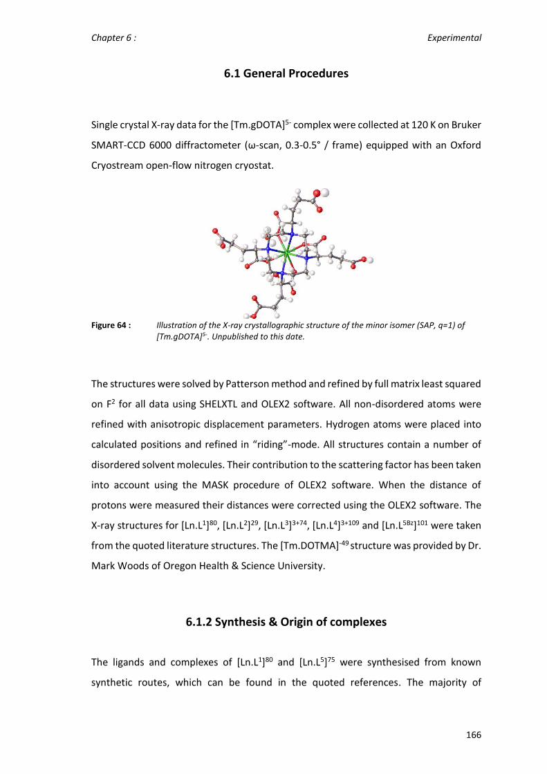
Chapter 6 : Experimental
166
6.1 General Procedures
Single crystal X-ray data for the [Tm.gDOTA]5- complex were collected at 120 K on Bruker
SMART-CCD 6000 diffractometer (ω-scan, 0.3-0.5° / frame) equipped with an Oxford
Cryostream open-flow nitrogen cryostat.
Figure 64 : Illustration of the X-ray crystallographic structure of the minor isomer (SAP, q=1) of [Tm.gDOTA]5-. Unpublished to this date.
The structures were solved by Patterson method and refined by full matrix least squared
on F2 for all data using SHELXTL and OLEX2 software. All non-disordered atoms were
refined with anisotropic displacement parameters. Hydrogen atoms were placed into
calculated positions and refined in “riding”-mode. All structures contain a number of
disordered solvent molecules. Their contribution to the scattering factor has been taken
into account using the MASK procedure of OLEX2 software. When the distance of
protons were measured their distances were corrected using the OLEX2 software. The
X-ray structures for [Ln.L1]80, [Ln.L2]29, [Ln.L3]3+74, [Ln.L4]3+109 and [Ln.L5Bz]101 were taken
from the quoted literature structures. The [Tm.DOTMA]-49 structure was provided by Dr.
Mark Woods of Oregon Health & Science University.
6.1.2 Synthesis & Origin of complexes
The ligands and complexes of [Ln.L1]80 and [Ln.L5]75 were synthesised from known
synthetic routes, which can be found in the quoted references. The majority of

Chapter 6 : Experimental
167
complexes and their synthetic procedures have been published before or during the
course of this PhD: [Ln.L1] 80 and [Ln.L5]- 75 were synthesised from known routes, [Ln.L2]
prepared by Dr. James Walton29, [Ln.L3]3+ prepared by Emily Neil74, [Ln.L4]3+ was
complexed from the ligand provided by Dr. Kanthi Senanayake109, [Ln.L5Bz]- was available
from previous synthesis by Dr. Kanthi Senanyake75 , [Ln.L6]110, [Ln.L7], [Ln.L7S] and [Ln.L9]+
prepared by Dr. Peter Harvey46, [Ln.L10] prepared by Dr. Brian McMahon61.
[Tm.DOTMA]- was provided by Dr. Mauro Botta49 and [Ln.gDOTA]5- was synthesised
from known routes with the help of Dr. Neil Sim111. The complex series [Ln.L8], [Ln.L8CO]
and [Ln.L11] are unpublished to this date and were prepared by Dr. Kanthi Senanayake
at Durham University. An overview of the structures is given in Scheme 17.

Chapter 6 : Experimental
168
Scheme 17 : Structures of all complexes analysed in this discussion.

Chapter 6 : Experimental
169
6.1.3 General NMR procedures
1H, 19F and 31P NMR spectra were obtained at 295 K (unless stated otherwise) on Varian
spectrometers operating at 4.7, 9.4, 11.7, 14.1, 16.5 Tesla, specifically on a Mercury 200
spectrometer (1H at 200.057 MHz, 19F at 188.242 MHz, 31P at 80.985 MHz), a Mercury
400 spectrometer (1H at 399.97 MHz, 19F at 376.331 MHz, 31P at 161.910 MHz), a Varian
Inova-500 spectrometer (1H at 499.78 MHz, 19F at 470.322 MHz, 31P at 202.340 MHz), a
Varian VNMRS-600 spectrometer (1H at 599.944 MHz, 19F at 564.511 MHz, 31P at
242.862 MHz) and a Varian VNMRS-700 spectrometer (1H at 700.000 MHz, 19F at
658.658 MHz, 31P at 283.365 MHz). Commercially available deuterated solvents were
used.
The operating temperature of the spectrometers was measured with the aid of an
internal calibration sample of neat ethylene glycol for high temperature studies. A
calibration sample of neat methanol was used for low temperatures studies. The
operating temperature of each spectrometer was measured before each set of
measurements of relaxation data.
The 19F and 31P relaxation data were measured without proton decoupling. The 31P
chemical shifts are reported relative to 85 % phosphoric acid. The 19F chemical shifts are
reported relative to fluorotrichloromethane.
The recorded free induction decays were processed using backward linear prediction,
optimal exponential weighting, zero-filling, Fourier transform, phasing and baseline
correction (by Whittaker smoothing), if necessary.
6.2 Relaxation data analysis
The nuclear relaxation times of the nuclei of interest were measured at the five different
fields mentioned above. The T1 values were measured using the inversion-recovery
technique. At first a crude T1 value was obtained, which was then used as the initial
guess in multiple repeat experiments. The incremented delay time was set to show full

Chapter 6 : Experimental
170
inversion and full recovery to equilibrium of the signal, which is roughly achieved at five
times the T1 value.
The line width and T2 data were obtained by Lorentzian line fitting. Due to the broad
nature of the resonances, the field inhomogeneity is negligible and it can be assumed
that in the absence of exchange broadening the T2* measured from the line width
corresponds to the actual T2 value.24
The lanthanide(III) complexes of [Ln.L2] and [Ln.L3]3+ were analysed in CD3OD, the
remaining complexes series were analysed in D2O solutions, unless stated otherwise.
The concentration of a sample was kept constant throughout a series of measurements,
which was in the range of 0.1 to 1 mM. An additional experiment was performed on
[Ln.L4]3+ to study the effect of different solvents on R1 and T1e. The longitudinal nuclear
relaxation rates varied as a function of the solvent, as the viscosity affected the
rotational correlation time, τR. However, the electronic relaxation times did not vary
with solvent within their estimated experimental errors (Table 38).
Table 38 : Estimated values of the electronic relaxation times of [Ln.L4]3+ using single resonance fitting (fixed µeff) in three different solvents (295 K).
Ln3+ D2O CD3OD MeCN
T1e / ps T1e / ps T1e / ps
Tb 0.54 ±0.06 0.50 ±0.05 0.52 ±0.07
Dy 0.43 ±0.03 0.41 ±0.04
Ho 0.34 ±0.01 0.22 ±0.06
Tm 0.20 ±0.02 0.19 ±0.04
Yb 0.17 ±0.03 0.16 ±0.03 0.15 ±0.03
τR / ps 350 ±28 253 ±17 162 ±12
For each complex studied, the 1H, 19F and 31P relaxation data measured and used for all
complexes can be found in Appendix 2.
The measured nuclear relaxation data was fitted by using a modified Matlab algorithm
originally written by Dr. Ilya Kuprov of Southampton University (original code shown in
Appendix 2, A24). The algorithm uses the Solomon-Morgan-Bloembergen equations (4)
to fit the measured relaxation data using the Matlab internal Levenberg-Marquardt

Chapter 6 : Experimental
171
minimisation of the non-linear squares error function. The results were analysed
iteratively. It was assumed that the longitudinal and transverse electronic relaxation
times were of a similar magnitude.
𝑅1 =2
15 (
µ0
4π)
2
γN
2 𝑔𝐿𝑛2 µ𝐵
2 𝐽 (𝐽 + 1)
𝑟6 [3
𝑇1𝑒
1 + 𝜔𝑁2 𝑇1𝑒
2 + 7𝑇2𝑒
1 + 𝜔𝑒2 𝑇2𝑒
2 ]
+2
5(
μ0
4π)
2 𝜔𝑁2 µ𝑒𝑓𝑓
4
(3kB𝑇)2 𝑟6[3
𝜏𝑟
1 + 𝜔𝑁2 𝜏𝑟
2] (4)
Some parameters were used globally for every lanthanide(III) complex in the series and
others were used for each complex individually. The rotational correlation time, τr, was
considered not to vary across a given series of complexes. An estimate for τr was
determined by the Stokes-Einstein Law. An estimate of the hydrodynamic radius, r, was
made by inspecting the X-ray data; in each case a reasonable agreement was found
(± 0.2 Å). DFT calculations were performed by Dr. Ilya Kuprov for further analysis of
internuclear distances and rotational correlation times.11 A full discussion is provided in
chapter 2, section 2.1.
The magnetic moments estimated for the fitting were taken from literature.11 The
majority of the global fitting curves and the nuclear relaxation data are shown in the
main chapters or in the Appendix 2.
6.2.1 Error Analysis
Each relaxation measurement was repeated at least three times and the mean value
recorded. The number of transients used in the measurements was determined by the
signal-to-noise ratio and also by the linewitdh of the resonance of interest. In each case,
the signal was fully recovered during the inversion-recovery sequence.
An experiment was performed to calculate the error associated with the temperature
variance of the spectrometers. The relaxation rate of [Tm.L1] was measured at five

Chapter 6 : Experimental
172
different temperatures (295 – 303 K in 2 K steps). At each measurement, the
temperature was also determined by using the temperature calibration sample
(ethylene glycol). According to the Solomon-Morgan-Bloembergen equations, the
temperature dependence of the relaxation rate, R1, is 1 / T2. At a variation of 0.5 K the
error was found to be less than 1.3 %. This was assumed to be similar for each complex
studied (Appendix 2, SI-Table 16).
A statistical error analysis was undertaken to determine the fitting errors. The
experimental errors of the measured relaxation rates were combined and used to
perturb the relaxation rates for each complex at each field. These perturbed rates
together with the unperturbed relaxation rates were used in a statistical error analysis
to obtain the error values for the individual parameters (µeff, r, τr and T1e) calculated in
the fitting process.112 An example of the obtained estimates is given inTable 10.
6.3 Pseudocontact shift analysis
The 1H NMR spectra for the complexes [Ln.L1-5,10] were fully characterised and analysed.
The full shift data can be found in the data tables in Appendix 3. The complex series
[Ln.L6-9,11] were only partially analysed as the attention was given to specific reporter
groups (e.g. tBu, CF3), due to varying amounts of available sample material and more
difficult analysis in the low symmetry complexes.
The accurate measurement of the chemical shift of a given resonance was performed
on the 9.4 Tesla Mercury 400 spectrometer, unless stated otherwise.
The observed shifts were tested for changes due to the bulk magnetic susceptibility shift
of the lanthanide(III) complexes. Using a coaxial insert tube containing a tert-butanol
reference (1%), it was found that over the concentration range used here (0.1 – 1 mM),
the BMS alteration to the observable shift was less than 0.2 ppm. The data is given in
Appendix 4. Considering that the observed shift range can vary from +500 ppm to -
500ppm in these paramagnetic complexes, this small effect can be largely neglected at
the concentrations used here.

Chapter 6 : Experimental
173
6.3.1 Variable temperature NMR studies
The variable temperatures 1H and 19F NMR resonances (D2O except [Ln.L2] and [Ln.L3]3+
(CD3OD)) of most complexes were measured as a function of the temperature on the
Varian VNMRS-600 spectrometer, with a few exceptions run on the Varian VNMRS-700
spectrometer, as stated in the discussion. However, the VT experiments on [Tm.L4] were
performed on the Varian Inova-500 spectrometer, due to restrictions for lowering the
temperature on the other high field spectrometers. In each measurement, the
temperature was measured with the internal calibration standard (ethylene glycol or
methanol) to ensure accurate temperature measurements. The error for the shift per
unit Kelvin was calculated using linear regression.
6.4 Bulk magnetic susceptibility measurements
The 1H NMR (D2O, except CD3OD for [Ln.L2]) spectra for the bulk magnetic susceptibility
(BMS) measurements were recorded at 295, 300 and 305 K using a coaxial insert
reference tube. A solution of D2O and tert-butanol (1%) was placed in the coaxial insert
tube, while the solution of the paramagnetic complexes was placed in the outer tube.
The sample was shimmed and locked to the D2O signal.
∆𝛿 =1000 𝑀 𝜒𝑀
𝑝𝑎𝑟𝑎
3 (10)
𝜇𝑒𝑓𝑓2 =
𝜒𝑀𝑝𝑎𝑟𝑎
3𝑘𝐵𝑇
𝑁𝐴𝜇0 (11)
The 1H NMR spectrum revealed the BMS shift between the diamagnetic reference and
the paramagnetic sample of the tert-butanol signal. From the BMS shift, the magnetic
susceptibility and the effective magnetic moment were calculated, as described in the
main text above (chapter 4, section 4.2.2 , and using equation 10 and 11). The
concentrations of each complex used in the calculations were obtained from ICP-MS
analysis of the complexes. The errors were calculated by performing repeat
measurements and the associated error was carried through the calculations. The

Chapter 6 : Experimental
174
temperature error, as shown above, was smaller than the experimental error. An
example for the estimation of the errors is given in Table 39, which was then combined
with the error of the concentration measurement.
Table 39 : Example of the error analysis for [Gd.L5Bz]- (three different temperatures for three different runs) used to estimate the experimental error (11.7 T, D2O).
T Δδ / ppm 𝜒𝑀𝑝𝑎𝑟𝑎/ m3 mol-1 µeff / BM
Run 1
295 K 0.15 3.64 8.30
300 K 0.14 3.56 8.29
305 K 0.14 3.49 8.27
Run 2
295 K 0.14 3.56 8.22
300 K 0.14 3.49 8.20
305 K 0.14 3.39 8.15
Run 3
295 K 0.12 3.54 8.19
300 K 0.14 3.46 8.17
305 K 0.14 3.41 8.18
6.5 SQUID magnetic susceptibility measurements
The SQUID measurements were performed by Dr. Johan Buurma in the Durham
University Chemistry department. The instrument used is Quantum Design RC- SQUID
magnetometer operating from 1.8 to 300 K. The samples were measured at a magnetic
field strength of 0.5 T.
A diamagnetic correction was performed on the structure of the complexes, but was
found to be negligible, as the lanthanide(III) ion moment is large (< 2% error).
The Curie constant was determined independently and was found to be in agreement
with the calculation derived from the Curie-Weiss fit. The absence of hysteresis was

Chapter 6 : Experimental
175
noted and it was concluded that were no ferromagnetic impurities. Example data for
[Gd.L5Bz] is given in Figure 61, similar behaviour was observed in the other samples.
A variety of experiments was performed to establish the consistency of the experiment.
For example, the [Gd.L5Bz] sample was prepared with different weights, and the
experiment was run at different induced magnetic field strengths. In every case the
calculated values were consistent, within the estimated error
𝜒−1 = 𝑇 − 𝜃
𝐶 (12)
The principal error of the measurement comes from the statistical error in the Curie
Weiss fit (from equation (12) and was determined using linear regression.

Dissecting the theories of lanthanide magnetic resonance References
176
7. References
(1) Bloembergen, N.; Morgan, L. O. J Chem Phys 1961, 34, 842–850. (2) Bleaney, B. J Magn Reson 1972, 8, 91–100. (3) Golding, R. M.; Pyykkö, P. Mol. Phys. 1973, 26, 1389–1396. (4) Solomon, I. Phys Rev 1955, 99, 559–565. (5) Bloembergen, N. J Chem Phys 1957, 27, 572–573. (6) McQueen, F. M. Rheumatology 2000, 39, 700–706. (7) Caravan, P.; Ellison, J. J.; McMurry, T. J.; Lauffer, R. B. Chem Rev 1999, 99, 2293–2352. (8) Kaltsoyannis, N.; Scott, P. The f elements; Oxford Chemistry Primers; Oxford University
Press: New York, 1999. (9) Binnemans, K.; Görller-Walrand, C. Chem. Phys. Lett. 1995, 245, 75–78. (10) Görller-Walrand, C.; Binnemans, K. In Handbook on the Physics and Chemistry of Rare
Earths; Karl A. Gschneidner, J. and L. E., Ed.; Elsevier, 1996; Vol. Volume 23, pp. 121–283. (11) Chalmers, K. H.; De Luca, E.; Hogg, N. H. M.; Kenwright, A. M.; Kuprov, I.; Parker, D.;
Botta, M.; Wilson, J. I.; Blamire, A. M. Chem Eur J 2010, 16, 134–148. (12) Newman, D. J.; Ng, B. Crystal field handbook /edited by D.J. Newman and Betty Ng;
Cambridge University Press: Cambridge, 2000. (13) Duan, C.-K.; Tanner, P. A. J. Phys. Chem. A 2010, 114, 6055–6062. (14) Carr, R. Lanthanide Complexes as Chiral Probes Exploiting Circularly Polarized
Luminescence. Doctoral, Durham University, 2014. (15) Parker, D.; Puschmann, H.; Batsanov, A. S.; Senanayake, K. Inorg Chem 2003, 42, 8646–
8651. (16) Walton, J. W.; Bari, L. D.; Parker, D.; Pescitelli, G.; Puschmann, H.; Yufit, D. S. Chem
Commun 2011, 47, 12289–12291. (17) Bertini, I.; Luchinat, C.; Parigi, G. Prog. Nucl. Magn. Reson. Spectrosc. 2002, 40, 249–273. (18) Bertini, I.; Calderone, V.; Cerofolini, L.; Fragai, M.; Geraldes, C. F. G. C.; Hermann, P.;
Luchinat, C.; Parigi, G.; Teixeira, J. M. C. FEBS Lett. 2012, 586, 557–567. (19) S. Dickins, R.; Parker, D.; I. Bruce, J.; J. Tozer, D. J Chem Soc Dalton Trans 2003, 1264–
1271. (20) Ren J, S. A. J Magn Reson B 1996, 111, 178–182. (21) Keeler, J. Understanding NMR Spectroscopy; John Wiley & Sons Ltd: Chichester, England,
2005. (22) Levitt, M. Spin Dynamics; John Wiley & Sons Ltd.: Chichester, 2001; Vol. 1. (23) Harvey, P.; Kuprov, I.; Parker, D. Eur J Inorg Chem 2012, 12, 2015–2022. (24) Bertini, I.; Luchinat, C.; Parigi, G. Solution NMR of Paramagnetic Molecules; Current
Methods in Inorganic Chemistry; Elsevier Science B.V.: Amsterdam, 2001; Vol. 2. (25) Sigel, A.; Sigel, H. Metal Ions in biological systems; The lanthanides and their
interrelations with biosystems; Marcel Dekker, Inc.: Netherlands, 2003; Vol. 40. (26) Thomsen, H. S. Radiol. Clin. North Am. 2009, 47, 827–831. (27) Kowalewski, J.; Luchinat, C.; Nilsson, T.; Parigi, G. J Phys Chem A 2002, 106, 7376–7382. (28) Bertini, I.; Capozzi, F.; Luchinat, C.; Nicastro, G.; Xia, Z. J Phys Chem 1993, 97, 6351–6354. (29) Walton, J. W.; Carr, R.; Evans, N. H.; Funk, A. M.; Kenwright, A. M.; Parker, D.; Yufit, D. S.;
Botta, M.; De Pinto, S.; Wong, K.-L. Inorg. Chem. 2012, 51, 8042–8056. (30) Aime, S.; Botta, M.; Fasano, M.; Crich, S. G.; Terreno, E. J. Biol. Inorg. Chem. 1996, 1, 312–
319. (31) Botta, M. Eur. J. Inorg. Chem. 2000, 399–407. (32) Geraldes, C. F. G. C.; Laurent, S. Contrast Media Mol. Imaging 2009, 4, 1–23.

Dissecting the theories of lanthanide magnetic resonance References
177
(33) Geraldes, C. F. G. C.; Urbano, A. M.; Alpoim, M. C.; Sherry, A. D.; Kuan, K.-T.; Rajagopalan, R.; Maton, F.; Muller, R. N. Magn. Reson. Imaging 1995, 13, 401–420.
(34) Caravan, P. Chem. Soc. Rev. 2006, 35, 512–523. (35) Nivorozhkin, A. L.; Kolodziej, A. F.; Caravan, P.; Greenfield, M. T.; Lauffer, R. B.; McMurry,
T. J. Angew. Chem. Int. Ed. 2001, 40, 2903–2906. (36) Aime, S.; Barge, A.; Delli Castelli, D.; Fedeli, F.; Mortillaro, A.; Nielsen, F. U.; Terreno, E.
Magn. Reson. Med. 2002, 47, 639–648. (37) Langereis, S.; Keupp, J.; van Velthoven, J. L. J.; de Roos, I. H. C.; Burdinski, D.; Pikkemaat,
J. A.; Grüll, H. J. Am. Chem. Soc. 2009, 131, 1380–1381. (38) Heffern, M. C.; Matosziuk, L. M.; Meade, T. J. Chem. Rev. 2014, 114, 4496–4539. (39) Liu, G.; Song, X.; Chan, K. W.; McMahon, M. T. NMR Biomed 2013, 26, 810–828. (40) Li, A. X.; Wojciechowski, F.; Suchy, M.; Jones, C. K.; Hudson, R. H. E.; Menon, R. S.; Bartha,
R. Magn. Reson. Med. 2008, 59, 374–381. (41) Vinogradov, E.; Sherry, A. D.; Lenkinski, R. E. J. Magn. Reson. 2013, 229, 155–172. (42) Vinogradov, E.; Soesbe, T. C.; Balschi, J. A.; Dean Sherry, A.; Lenkinski, R. E. J. Magn.
Reson. 2012, 215, 64–73. (43) Chalmers, K. H.; Kenwright, A. M.; Parker, D.; Blamire, A. M. Magn Reson Med 2011, 66,
931–936. (44) Chalmers, K. H.; Botta, M.; Parker, D. J Chem Soc Dalton Trans 2011, 40, 904–913. (45) Meyerspeer, M.; Robinson, S.; Nabuurs, C. I.; Scheenen, T.; Schoisengeier, A.; Unger, E.;
Kemp, G. J.; Moser, E. Magn Reson Med 2012, 1713–1723. (46) Harvey, P.; Blamire, A. M.; Wilson, J. I.; Finney, K.-L. N. A.; Funk, A. M.; Senanayake, P. K.;
Parker, D. Chem Sci 2013, 4, 4251–4258. (47) Hekmatyar, S. K.; Hopewell, P.; Pakin, S. K.; Babsky, A.; Bansal, N. Magn Reson Med 2005,
53, 294–303. (48) Geraldes, C. F. G. C.; Sherry, A. D.; Kiefer, G. E. J Magn Reson 1992, 97, 290–304. (49) Aime, S.; Botta, M.; Garda, Z.; Kucera, B. E.; Tircso, G.; Young, V. G.; Woods, M. Inorg.
Chem. 2011, 50, 7955–7965. (50) Pakin, S. K.; Hekmatyar, S. K.; Hopewell, P.; Babsky, A.; Bansal, N. NMR Biomed 2006, 19,
116–124. (51) Schmid, F.; Höltke, C.; Parker, D.; Faber, C. Magn. Reson. Med. 2013, 69, 1056–1062. (52) Keizers, P. H. J.; Ubbink, M. Prog. Nucl. Magn. Reson. Spectrosc. 2011, 58, 88–96. (53) Madl, T.; Güttler, T.; Görlich, D.; Sattler, M. Angew. Chem. Int. Ed. 2011, 50, 3993–3997. (54) Otting, G. J. Biomol. NMR 2008, 42, 1–9. (55) Graham, B.; Loh, C. T.; Swarbrick, J. D.; Ung, P.; Shin, J.; Yagi, H.; Jia, X.; Chhabra, S.;
Barlow, N.; Pintacuda, G.; Huber, T.; Otting, G. Bioconjug. Chem. 2011, 22, 2118–2125. (56) Keizers, P. H. J.; Saragliadis, A.; Hiruma, Y.; Overhand, M.; Ubbink, M. J. Am. Chem. Soc.
2008, 130, 14802–14812. (57) Otting, G. Annu. Rev. Biophys. 2010, 39, 387–405. (58) Madl, T.; Bermel, W.; Zangger, K. Angew. Chem. Int. Ed. 2009, 48, 8259–8262. (59) Downing, A. K. Protein Nuclear Magnetic Resonance Techniques; Springer Science &
Business Media, 2004. (60) Berry, M. T.; Schwieters, C.; Richardson, F. S. J Chem Phys 1988, 122, 105–124. (61) Gempf, K. L.; Butler, S. J.; Funk, A. M.; Parker, D. Chem Commun 2013, 49, 9104–9106. (62) McGarvey, B. R. J. Magn. Reson. 1969 1979, 33, 445–455. (63) Fries, P. H.; Belorizky, E. J Chem Phys 2007, 126, 204503–204513. (64) Goldman, M. J Magn Reson 2001, 149, 160–187. (65) Zuo, C. S.; Mahmood, A.; Sherry, A. D. J Magn Reson 2001, 151, 101–106. (66) Alsaadi, B. M.; Rossotti, F. J. C.; Williams, R. J. P. J Chem Soc Dalton Trans 1980, 2147–
2150.

Dissecting the theories of lanthanide magnetic resonance References
178
(67) Alsaadi, B. M.; Rossotti, F. J. C.; Williams, R. J. P. J Chem Soc Dalton Trans 1980, 2151–2154.
(68) Aime, S.; Barbero, L.; Botta, M.; Ermondi, G. J Chem Soc Dalton Trans 2 1992, 225–228. (69) Einstein, A. Ann. Phys. 1905, 322, 549–560. (70) Wittebort, R. J.; Szabo, A.; Gurd, F. R. N. J Am Chem Soc 1980, 102, 5723–5728. (71) Lipari, G.; Szabo, A. J Am Chem Soc 1982, 104, 4546–4559. (72) Fries, P. H.; Belorizky, E. J Chem Phys 2012, 136, 074513–10. (73) Fries, P. H.; Belorizky, E. J Chem Phys 2005, 123, 124510–124515. (74) Neil, E. R.; Funk, A. M.; Yufit, D. S.; Parker, D. Dalton Trans 2014, 5490–5504. (75) Broan, C. J.; Cole, E.; Jankowski, K. J.; Parker, D.; Pulukkody, K.; Boyce, B. A.; Beeley, N. R.
A.; Millar, K.; Millican, A. T. Synthesis 1992, 1992, 63–68. (76) Mironov, V. S.; Galyametdinov, Y. G.; Ceulemans, A.; Görller-Walrand, C.; Binnemans, K. J
Chem Phys 2002, 116, 4673–4685. (77) Mironov, V. S.; Galyametdinov, Y. G.; Ceulemans, A.; Görller-Walrand, C.; Binnemans, K.
Chem. Phys. Lett. 2001, 345, 132–140. (78) Ren, J.; Zhang, S.; Dean Sherry, A.; Geraldes, C. F. G. C. Inorganica Chim. Acta 2002, 339,
273–282. (79) Evans, D. F. J. Chem. Soc. Resumed 1959, 2003–2005. (80) Nocton, G.; Nonat, A.; Gateau, C.; Mazzanti, M. Helv. Chim. Acta 2009, 92, 2257–2273. (81) Shannon, R. D. Acta Crystallogr. Sect. A 1976, 32, 751–767. (82) Funk, A. M.; Fries, P. H.; Harvey, P.; Kenwright, A. M.; Parker, D. J Phys Chem A 2013, 117,
905–917. (83) Kang, J.-G.; Kim, Tack-Jin. Bull Korean Chem Soc 2005, 26, 1057–1064. (84) Bertini, I.; Luchinat, C.; Turano, P.; Battaini, G.; Casella, L. Chem. – Eur. J. 2003, 9, 2316–
2322. (85) Bleaney, B. J Magn Reson 1972, 8, 94. (86) Rinehart, J. D.; Long, J. R. Chem. Sci. 2011, 2, 2078–2085. (87) Aime, S.; Botta, M.; Ermondi, G. Inorg Chem 1992, 31, 4291–4299. (88) Aime, S.; Botta, M.; Parker, D.; Williams, J. A. G. J Chem Soc Dalton Trans 1995, 2259–
2266. (89) Di Pietro, S.; Piano, S. L.; Di Bari, L. Coord. Chem. Rev. 2011, 255, 2810–2820. (90) Boulon, M.-E.; Cucinotta, G.; Luzon, J.; Degl’Innocenti, C.; Perfetti, M.; Bernot, K.; Calvez,
G.; Caneschi, A.; Sessoli, R. Angew. Chem. Int. Ed. 2013, 52, 350–354. (91) Cucinotta, G.; Perfetti, M.; Luzon, J.; Etienne, M.; Car, P.-E.; Caneschi, A.; Calvez, G.;
Bernot, K.; Sessoli, R. Angew. Chem. Int. Ed. 2012, 51, 1606–1610. (92) Souza, A. S.; Couto dos Santos, M. A. Chem. Phys. Lett. 2012, 521, 138–141. (93) Jensen, J.; Mackintosh, A. R. Rare Earth Magnetism; The international series of
mongraphs of physics; Clarendon Press: Oxford, 1991. (94) Ma, C.-G.; Brik, M. G.; Kiisk, V.; Kangur, T.; Sildos, I. J. Alloys Compd. 2011, 509, 3441–
3451. (95) Auzel, F.; Malta, O. L. J. Phys. 1983, 44, 201–206. (96) Malta, O. L.; Antic-Fidancev, E.; Lemaitre-Blaise, M.; Milicic-Tang, A.; Taibi, M. J. Alloys
Compd. 1995, 228, 41–44. (97) Ashcroft, N. W.; Mermin, N. D. Solid state physics; Saunders College, 1976. (98) Evans, D. F.; James, T. A. J. Chem. Soc. Dalton Trans. 1979, 723–726. (99) Sur, S. K. J. Magn. Reson. 1969 1989, 82, 169–173. (100) Corsi, D. M.; Platas-Iglesias, C.; Bekkum, H. van; Peters, J. A. Magn. Reson. Chem. 2001,
39, 723–726. (101) Aime, S.; Batsanov, A. S.; Botta, M.; Dickins, R. S.; Faulkner, S.; Foster, C. E.; Harrison,
A.; Howard, J. A. K.; Moloney, J. M.; Norman, T. J.; Parker, D.; Royle, L.; Williams, J. A. G. J. Chem. Soc. Dalton Trans. 1997, 3623–3636.

Dissecting the theories of lanthanide magnetic resonance References
179
(102) Lacheisserie, E. du T. de; Gignoux, D.; Schlenker, M. Magnetism: Materials and Applications; Springer Science & Business Media, 2005.
(103) Bünzli, J.-C. G.; Piguet, C. Chem. Soc. Rev. 2005, 34, 1048–1077. (104) Kim, J.-G.; Yoon, S.-K.; Sohn, Y.; Kang, J.-G. J Alloys Compd 1998, 274, 1–9. (105) Kang, J.-G.; Na, M.-K.; Yoon, S.-K.; Sohn, Y.; Kim, Y.-D.; Suh, I.-H. Inorg Chim Acta 2000,
310, 56–64. (106) Gruber, J. B.; Leavitt, R. P.; Morrison, C. A.; Chang, N. C. J Chem Phys 1985, 82, 5373–
5378. (107) Liusen, H.; Michael, F. R.; Chang-Kui, D.; Shangda, X.; Min, Y. J. Phys. Condens. Matter
2011, 23, 045501. (108) Charnock, G. T. P.; Kuprov, I. Phys. Chem. Chem. Phys. 2014, 16, 20184–20189. (109) Dickins, R. S.; Howard, J. A. K.; Maupin, C. L.; Moloney, J. M.; Parker, D.; Riehl, J. P.;
Siligardi, G.; Williams, J. A. G. Chem Eur J 1999, 5, 1095–1105. (110) Harvey, P. Paramagnetic Probes for Magnetic Resonance. Doctoral, Durham
University, 2013. (111) Woods, M.; Aime, S.; Botta, M.; Howard, J. A. K.; Moloney, J. M.; Navet, M.; Parker, D.;
Port, M.; Rousseaux, O. J. Am. Chem. Soc. 2000, 122, 9781–9792. (112) Motulsky, H.; Christopoulos, A. Fitting Models to Biological Data Using Linear and
Nonlinear Regression: A Practical Guide to Curve Fitting; Oxford University Press, 2004.

Dissecting the theories of lanthanide magnetic resonance Appendices
A
Appendices
The following appendices contain all the relaxation and shift data that lead to the values
presented in the main text. The Appendices follow the order of the lanthanide(III) series
for each discussion chapter.
Appendix 1 : List of complexes used A2
Appendix 2 : Electronic relaxation times through the analysis of nuclear
relaxation rates
[Ln.L1]
[Ln.L2]
[Ln.L3]3+
[Ln.L4]3+
[Ln.L5]-
[Ln.L6] + [Ln.L6C]
[Ln.L7]
[Ln.L8]
[Ln.L9]+
[Ln.L10]
[Ln.L11]
[Ln.gDOTA]5-
[Tm.DOTMA]-
Shift ranges
Fitting algorithm
A4
A6
A9
A11
A13
A15
A17
A17
A18
A18
A21
A22
A23
A23
A24

Dissecting the theories of lanthanide magnetic resonance Appendices
A
Appendix 3 : The discrepancies in Bleaney’s theory of magnetic resonance
[Ln.L1]
[Ln.L2]
[Ln.L3]3+
[Ln.L4]3+
[Ln.L5]-
[Ln.L6]
[Ln.L7-9]
[Ln.L10]
[Ln.L11]
[Tm.DOTMA]-
A27
A28
A30
A31
A32
A33
A34
A35
A36
A37
Appendix 4 : The effect of J-mixing on the magnetic susceptibility
[Ln.L2]
[Ln.L5]- + [Ln.L5Bz]-
[Ln.L10]
[Ln.gDOTA]5-
[Ln.DOTMA]-
A39
A40
A41
A42
A43
Appendix 5 : List of publications A44

Dissecting the theories of lanthanide magnetic resonance Appendix 1
A1
Appendix 1 : List of examined complexes

Dissecting the theories of lanthanide magnetic resonance Appendix 2
A2
SI-Figure 1 : Structures of all complexes examined in this discussion

Dissecting the theories of lanthanide magnetic resonance Appendix 2
A3
Appendix 2 : Electronic Relaxation times estimated
through analysis of nuclear relaxation rates

Dissecting the theories of lanthanide magnetic resonance Appendix 2
A4
SI-Table 1 : 1H nuclear relaxation rates,R1, and single fitting values (µeff = 9.8 BM) for [Tb.L1] (295 K, D2O).
1H R1/ s-1 Fitting values
4.7 T 9.4 T 11.7 T 14.1 T 16.5 T r / Å τR / ps T1e / ps
pyH4 44 ±3 85 ±5 131 ±21 152 ±7 177 ±12 6.48 196.5 0.19 pyH3 108 ±6 195 ±5 258 ±5 316 ±9 390 ±15 5.58 124.0 0.29 Hax’ 499 ±57 1027 ±55 1484 ±86 1639 ±149 1957 ±166 4.36 229.7 0.20 Heq 392 ±25 768 ±25 995 ±41 1268 ±50 1465 ±43 4.55 172.2 0.27 Hax 465 ±28 869 ±45 1155 ±59 1398 ±39 1607 ±50 4.51 195.3 0.30
pyCHN’ 403 ±11 714 ±45 1002 ±21 1346 ±30 1575 ±54 4.34 107.5 0.21
SI-Table 2 : 1H nuclear relaxation rates,R1, and single fitting values (µeff = 10.3 BM) for [Dy.L1] (295 K, D2O).
1H R1/ s-1 Fitting values
4.7 T 9.4 T 11.7 T 14.1 T 16.5 T r / Å τR / ps T1e / ps
pyH5 125 ±6 238 ±6 314 ±6 395 ±12 503 ±9 5.31 85.4 0.23 pyH4 64 ±2 126 ±1 164 ±2 211 ±3 258 ±3 6.15 121.6 0.26 pyH3 130 ±7 255 ±3 347 ±6 414 ±20 513 ±11 5.58 151.5 0.28 Heq 435 ±32 776 ±33 1252 ±37 1576 ±243 1787 ±42 4.50 156.3 0.20
SI-Table 3 : 1H nuclear relaxation rates,R1, and single fitting values (µeff = 10.4 BM) for [Ho.L1] (295 K, D2O).
1H R1/ s-1 Fitting values
4.7 T 9.4 T 11.7 T 14.1 T 16.5 T r / Å τR / ps T1e / ps
pyH5 91 ±6 210 ±6 305 ±26 382 ±13 509 ±26 5.21 75.8 0.12 pyH4 48 ±2 103 ±2 142 ±5 184 ±3 232 ±6 6.16 100.5 0.17 pyH3 92 ±11 298 ±27 283 ±51 423 ±51 538 ±51 5.47 125.1 0.18
pyCHN 362 ±10 819 ±30 1245 ±32 1556 ±43 1777 ±60 4.55 193.4 0.12

Dissecting the theories of lanthanide magnetic resonance Appendix 2
A5
SI-Table 4 : 1H nuclear relaxation rates,R1, and single fitting values (µeff = 9.4 BM) for [Er.L1] (295 K, D2O).
1H R1/ s-1 Fitting values
4.7 T 9.4 T 11.7 T 14.1 T 16.5 T r / Å τR / ps T1e / ps
pyH3 87 ±5 176 ±8 233 ±13 284 ±27 358 ±48 5.52 130.3 0.22 pyH4 39 ±2 68 ±3 88 ±4 119 ±2 140 ±3 6.34 105.5 0.24 pyH5 84 ±5 181 ±8 223 ±10 272 ±10 325 ±10 5.89 199.4 0.25 Heq 365 ±30 667 ±19 1137 ±47 1352 ±58 1666 ±196 4.40 148.1 0.17 Heq’ 389 ±20 657 ±48 1085 ±51 1281 ±67 1597 ±67 4.21 107.7 0.18
SI-Table 5: 1H nuclear relaxation rates,R1, and single fitting values (µeff = 7.6 BM) for [Tm.L1] (295 K, D2O).
1H R1/ s-1 Fitting values
4.7 T 9.4 T 11.7 T 14.1 T 16.5 T r / Å τR / ps T1e / ps
CHN’ 414 ±7 989±44 1431±33 1872±321 2295±108 3.48 132.5 0.07 pyH3/5 25 ±1 61 ±0.3 84 ±0.2 108 ±0.3 134 ±0.5 5.63 140.5 0.08 pyH4 12 ±0.2 27 ±0.2 37 ±0.1 48 ±0.2 60 ±0.3 6.36 116.6 0.09 Hax’ 400±19 971±51 1433±52 1745±143 2159±69 3.57 164.2 0.07 CHN 102±85 209 ±8 311 ±8 362 ±19 471 ±21 4.55 122.5 0.11 Heq 82 ±12 201 ±5 282 ±1 365 ±2 454 ±3 4.57 133.5 0.07 Heq’ 94 ±1 226 ±4 321 ±2 415 ±3 515 ±3 4.47 132.0 0.07 Hax 116 ±2 277 ±5 390 ±3 510 ±3 636 ±9 4.29 121.5 0.07
SI-Table 6 1H nuclear relaxation rates,R1, and single fitting values (µeff = 4.5 BM) for [Yb.L1] (295 K, D2O).
1H R1/ s-1 Fitting values
4.7 T 9.4 T 11.7 T 14.1 T 16.5 T r / Å τR / ps T1e / ps
pyCHN’ 89 ±1 159 ±2 210 ±3 257 ±4 311 ±4 3.41 134.7 0.06 pyH3 5.7 ±0.2 9.5 ±0.5 12.5 ±0.1 12.8 ±0.7 18.6 ±0.2 5.46 112.4 0.07 pyH4 3.1 ±0.1 4.8 ±0.2 5.8 ±0.1 7.4 ±0.4 8.4 ±0.1 6.29 128.7 0.10 pyH5 5.4 ±0.1 9.4 ±0.4 12.0 ±0.1 15.4 ±0.7 17.8 ±0.1 5.45 13.5 0.06 CHN 27 ±3 34 ±2 46 ±1 61 ±1 54 ±1 4.42 99.9 0.11 Heq 21 ±1 32 ±1 42 ±1 52 ±1 62 ±1 4.34 92.5 0.07 Heq’ 23 ±1 36 ±1 48 ±1 59 ±1 70 ±1 4.33 112.1 0.08 Hax 29 ±1 44 ±1 59 ±1 73 ±1 88 ±1 4.01 79.4 0.06
SI-Table 7 : Individual estimated values of the effective magnetic moment, µeff, the electronic relaxation time, T1e and the rotational correlation time, τR, using global fitting procedures for the quoted resonances of [Ln.L1] (295 K, D2O).
Ln3+ pyH3 pyH4
µeff / BM T1e / ps µeff / BM T1e / ps
Tb 9.63 0.29 9.67 0.24 Dy 10.38 0.29 10.56 0.28 Ho 10.55 0.18 10.34 0.17 Er 9.46 0.22 9.01 0.23
Tm 7.49 0.08 7.37 0.08 Yb 4.34 0.07 4.20 0.11
τR / ps 135.3 129.5

Dissecting the theories of lanthanide magnetic resonance Appendix 2
A6
SI-Table 8 : 1H nuclear relaxation rates, R1, and single fitting values (µeff = 9.8 BM) for [Tb.L2] (295 K, CD3OD).
1H R1/ s-1 Fitting values
4.7 T 9.4 T 11.7 T 14.1 T 16.5 T r / Å τR / ps T1e / ps
Hax’ 571 ±18 1178 ±12 1528 ±14 1834 ±22 2208 ±24 4.27 86.7 0.26 Hax 526 ±7 1090 ±11 1357 ±5 1687 ±15 2057 ±26 4.30 160.3 0.27 CHN 384 ±11 809 ±12 1022 ±6 1298 ±26 1550 ±26 4.50 164.8 0.24 PhH’ 34 ±1 69 ±1 89 ±1 107 ±1 127 ±1 6.88 194.8 0.27 PhH 14 ±0.1 27 ±1 35 ±1 41 ±1 49 ±1 8.08 196.5 0.31 pyH5 89 ±1 181 ±1 234 ±1 287 ±3 330 ±6 5.87 206.6 0.25 pyH4 43 ±1 87 ±1 109 ±1 133 ±1 153 ±1 6.68 214.9 0.28 pyH3 97 ±2 199 ±2 252 ±2 305 ±3 351 ±6 5.81 220.63 0.26 Heq 388 ±6 806 ±13 1031 ±12 1143 ±31 1471 ±27 4.59 189.6 0.29 CHN’ 1877 ±63 3253 ±125 4572 ±82 5848 ±230 6784 ±183 3.52 159.2 0.29
SI-Table 9 : 1H nuclear relaxation rates, R1, and single fitting values (µeff = 10.3 BM) for [Dy.L2] (295 K, CD3OD).
1H R1/ s-1 Fitting values
4.7 T 9.4 T 11.7 T 14.1 T 16.5 T r / Å τR / ps T1e / ps
Hax’ 787 ±25 1608 ±16 2058 ±7 2546 ±20 2895 ±71 4.22 212.8 0.28 Hax 710 ±27 1484 ±9 1848 ±5 2312 ±13 2593 ±45 4.30 225.6 0.27 PhH’ 46 ±1 93 ±1 131 ±4 149 ±2 182 ±2 6.69 19.5 0.26 PhH 20 ±1 37 ±1 52 ±1 59 ±1 72 ±1 7.81 181.0 0.32 pyH5 136 ±2 261 ±5 310 ±16 414 ±13 459 ±12 5.73 187.0 0.36 pyH3 150 ±2 282 ±5 344 ±7 455 ±7 518 ±11 5.59 213.6 0.35
SI-Table 10 : 1H nuclear relaxation rates, R1, and single fitting values (µeff = 10.4 BM) for [Ho.L2] (295 K, CD3OD).
1H R1/ s-1 Fitting values
4.7 T 9.4 T 11.7 T 14.1 T 16.5 T r / Å τR / ps T1e / ps
PhH 25 ±3 55 ±1 68 ±1 84 ±2 98 ±2 7.46 206.8 0.26 pyH5 94 ±4 199 ±10 278 ±19 394 ±25 482 ±25 5.21 72.4 0.12 pyH4 44 ±2 102 ±4 141 ±5 170 ±4 203 ±4 6.58 199.5 0.17 pyH3 92 ±4 218 ±13 299 ±8 382 ±8 433 ±16 5.78 207.0 0.14 Heq’ 458 ±7 1076 ±26 1367 ±37 1658 ±36 2166 ±38 4.38 135.9 0.23

Dissecting the theories of lanthanide magnetic resonance Appendix 2
A7
SI-Table 11 : 1H nuclear relaxation rates, R1, and single fitting values (µeff = 9.4 BM) for [Er.L2] (295 K, CD3OD).
1H R1/ s-1 Fitting values
4.7 T 9.4 T 11.7 T 14.1 T 16.5 T r / Å τR / ps T1e / ps
CHN’ 1893 ±32 3562 ±104 4391 ±44 5408 ±194 6592 ±271 3.43 181.6 0.24 pyH5 98 ±1 182 ±2 233 ±4 280 ±3 327 ±6 5.73 192.0 0.31 pyH3 107 ±2 192 ±2 245 ±3 295 ±3 343 ±6 5.69 188.3 0.33 pyH4 49 ±1 88 ±1 108 ±1 131 ±1 151 ±1 6.53 198.2 0.36 PhH’ 33 ±1 58 ±1 74 ±1 90 ±1 104 ±1 6.93 182.8 0.35 Hax 485 ±11 917 ±11 1184 34± 1427 ±39 1662 ±64 4.37 194.1 0.29 Heq 381 ±9 731 ±12 938 ±31 1120 ±33 1319 ±52 4.54 195.3 0.29 CHN 434 ±12 802 ±18 1048 ±30 1252 ±29 1473 ±49 4.45 185.5 0.30 Hax’ 553 ±14 1033 ±16 1314 ±31 1586 ±26 1832 ±13 4.30 200.0 0.31
SI-Table 12 : 1H nuclear relaxation rates, R1, and single fitting values (µeff = 7.6 BM) for [Tm.L2] (295
K, CD3OD).
1H R1/ s-1 Fitting values
4.7 T 9.4 T 11.7 T 14.1 T 16.5 T r / Å τR / ps T1e / ps
CHN’ 574±10 1304±35 1700±26 2133±16 2544±88 3.51 182.0 0.11 pyH3 30±1 69±0.3 92±1 116±1 139±1 5.68 174.1 0.10 pyH5 28±1 65±0.4 86±1 109±1 130±0.4 5.75 177.2 0.10 pyH4 13±0.4 31±0.2 40±0.2 50±0.2 56±0.1 6.61 243.9 0.08 Hax’ 517±18 1390±53 1550±26 1806±91 2459±25 3.56 178.6 0.14 CHN 120±1 287±3 398±2 495±1 558±13 4.49 227.2 0.06 Heq 104±1 244±2 333±1 415±1 475±12 4.63 215.1 0.08 Heq’ 114±1 261±3 360±2 442±1 504±14 4.59 221.6 0.08 Hax 133±2 323±3 430±3 542±1 631±6 4.42 205.0 0.08
SI-Table 13 : 1H nuclear relaxation rates, R1, and single fitting values (µeff = 4.5 BM) for [Yb.L2] (295 K, CD3OD).
1H R1/ s-1 Fitting values
4.7 T 9.4 T 11.7 T 14.1 T 16.5 T r / Å τR / ps T1e / ps
CHN’ 104 ±1 193 ±1 243 ±3 283 ±1 326 ±1 3.45 228.7 0.07 pyH3/5 6.2 ±0.1 10.5 ±0.5 12.7 ±0.1 15.0 ±0.1 17.1 ±0.1 5.68 214.3 0.09 pyH4 4.3 ±0.1 5.7 0.2± 6.5 ±0.1 7.4 ±0.1 8.3 ±0.1 6.58 193.2 0.18 CHN 23 ±2 43 ±1 54 ±1 66 ±1 79 ±1 4.34 161.4 0.07 Heq 23 ±2 37 ±1 46 ±1 55 ±1 63 ±1 4.57 174.1 0.10 Heq’ 27 ±1 42 ±1 52 ±1 62 ±1 70 ±1 4.51 178.4 0.11 Hax 33 ±1 51 ±1 64 ±1 75 ±1 87 ±1 4.34 162.2 0.11

Dissecting the theories of lanthanide magnetic resonance Appendix 2
A8
SI-Table 14 : 31P nuclear relaxation rates of [Ln.L2] used for global fitting (295 K, CD3OD).
Ln3+ δH / ppm R1/ s-1
4.7 T 9.4 T 11.7 T 14.1 T 16.5 T
Eu 16.6 2.5±0.1 7.5±0.2 10.5±0.1 13.9±0.1 18.1±0.1 Tb -35.7 242±3 603±11 824±4 1071±9 1322±11 Dy -15.9 332±10 876±15 1213±7 1619±27 1978±18 Ho -24.6 247±3 701±21 1026±3 1341±18 1709±19 Er -10.5 248±6 533±10 745±3 963±13 1202±10 Tm 8.4 64±1 194±6 271±2 358±3 463±3 Yb 17.7 11±0.3 24±0.4 34±0.2 42±0.2 54±0.1
SI-Table 15 : Individual estimated values of the effective magnetic moment, µeff, the electronic relaxation time, T1e and the rotational correlation time, τR, using global fitting procedures for the quoted resonances of [Ln.L2] (295 K, CD3OD).
Ln3+ Hax Heq pyH3 pyH5 31P
µeff / BM
T1e / ps
µeff / BM
T1e / ps
µeff / BM
T1e / ps
µeff / BM
T1e / ps
µeff / BM
T1e / ps
Tb 9.81 0.22 8.73 0.19 8.31 0.21 8.19 0.21 8.75 0.28 Dy 10.48 0.31 9.39 0.24 9.16 0.33 8.98 0.23 9.72 0.26 Ho 10.27 0.15 8.98 0.11 11.04 0.16 11.64 0.14 9.39 0.13 Er 9.28 0.27 8.29 0.24 10.18 0.38 10.43 0.41 8.50 0.31
Tm 7.34 0.10 8.92 0.16 8.22 0.09 8.34 0.13 6.76 0.06 Yb 4.15 0.14 5.25 0.13 4.67 0.11 4.80 0.12 3.84 0.07 τR / ps
207 130 203 131 328
SI-Table 16 31P relaxation rates at a range of temperature K for [Tm.L2], (CD3OD, 16.5 T, 1 mM).
R1 / s-1 T 1 / T2 x 10-3
463 295 0.0115 446 297 0.0114 426 299 0.0112 413 301 0.0111 397 302 0.0109

Dissecting the theories of lanthanide magnetic resonance Appendix 2
A9
SI-Table 17 : 1H nuclear relaxation rates,R1, and single fitting values (µeff = 9.8 BM) for [Tb.L3]3+ (295 K, CD3OD).
1H R1/ s-1 Fitting values
4.7 T 9.4 T 11.7 T 14.1 T 16.5 T r / Å τR / ps T1e / ps
Hax’ 793 ±45 1471 ±41 1828 ±25 2230 ±31 2574 ±58 4.18 198.1 0.35 Heq 336 ±7 668 ±28 880 ±20 999 ±36 1204 ±33 4.75 214.2 0.28 CH3 53 ±1 96 ±1 122 ±1 147 ±1 170 ±1 6.57 196.2 0.36 H 95 ±2 169 ±2 210 ±1 262 ±3 305 ±4 5.93 169.2 0.37
PhH 23 ±1 40 ±1 50 ±1 59 ±1 67 ±2 7.70 221.6 0.41 pyH4 46 ±3 93 ±1 122 ±1 148 ±2 168 ±3 6.56 220.0 0.24 pyH5 115 ±2 216 ±6 294 ±4 361 ±6 400 ±16 5.67 210.4 0.27 pyH3 122 ±3 226 ±4 305 ±7 365 ±8 433 ±10 5.59 174.4 0.30
SI-Table 18 : 1H nuclear relaxation rates,R1, and single fitting values (µeff = 10.3 BM) for [Dy.L3]3+ (295 K, CD3OD).
1H R1/ s-1 Fitting values
4.7 T 9.4 T 11.7 T 14.1 T 16.5 T r / Å τR / ps T1e / ps
PhH 23 ±1 40 ±3 49 ±1 61 ±2 69 ±3 7.89 195.5 0.45 PhH’ 29 ±1 53 ±2 70 ±1 84 ±1 99 ±2 7.40 180.5 0.36 pyH4 59 ±3 114 ±5 141 ±6 176 ±5 212 ±5 6.49 158.2 0.35 pyH3 94 ±3 187 ±5 249 ±15 315 ±10 385 ±22 5.79 133.5 0.26
SI-Table 19 : 1H nuclear relaxation rates,R1, and single fitting values (µeff = 10.4 BM) for [Ho.L3]3+ (295 K, CD3OD).
1H R1/ s-1 Fitting values
4.7 T 9.4 T 11.7 T 14.1 T 16.5 T r / Å τR / ps T1e / ps
Hax’ 721 ±51 1544 ±24 2299 ±123 2494 ±116 3252 ±93 4.15 173.6 0.21 Heq 328 ±7 830 ±37 1026 ±19 1216 ±31 1647 ±99 4.59 135.2 0.22 Heq’ 448 ±13 1044 ±47 1359 ±30 1531 ±66 1864 ±150 4.56 248.5 0.18 CH3 50 ±1 113 ±2 145 ±1 178 ±2 226 ±10 6.41 145.5 0.24 H 81 ±1 184 ±2 240 ±4 296 ±2 362 ±19 5.97 163.6 0.24
PhH’ 20 ±1 47 ±1 63 ±1 72 ±1 95 ±6 7.45 159.8 0.22 pyH3 112 ±4 262 ±10 378 ±6 405 ±9 475 ±46 5.67 238.5 0.15

Dissecting the theories of lanthanide magnetic resonance Appendix 2
A10
SI-Table 20 : 1H nuclear relaxation rates,R1, and single fitting values (µeff = 9.4 BM) for [Er.L3]3+ (295 K, CD3OD).
1H R1/ s-1 Fitting values
4.7 T 9.4 T 11.7 T 14.1 T 16.5 T r / Å τR / ps T1e / ps
pyH4 36 ±2 61 ±3 93 ±7 108 ±7 122 ±7 6.65 144.1 0.29 PhH 18 ±1 30 ±1 40 ±1 46 ±1 54 ±1 7.75 189.8 0.38 CH3 52 ±1 85 ±1 107 ±1 132 ±2 153 ±2 6.47 160.2 0.40
SI-Table 21 : 1H nuclear relaxation rates,R1, and single fitting values (µeff = 7.6 BM) for [Tm.L3]3+ (295
K, CD3OD).
1H R1/ s-1 Fitting values
4.7 T 9.4 T 11.7 T 14.1 T 16.5 T r / Å τR / ps T1e / ps
CHN’ 566±20 1413±97 1718±20 2088±43 2482±76 3.53 239.3 0.09 pyH3 31±0.3 75±2 105±1 125±2 149±2 5.62 213.9 0.07 pyH4 18±0.4 40±2 53±1 63±1 73±1 6.36 234.4 0.11 PhH’ 6±0.1 13±0.1 16±0.1 20±0.1 24±0.2 7.68 179.4 0.15 PhH 4±0.1 8±0.1 10±0.1 12±0.2 15±0.2 8.27 150.7 0.19
H 22±0.1 50±0.4 65±0.3 82±1 97±1 6.71 186.5 0.15 CH3 14±0.1 29±0.1 37±0.1 46±0.2 54±0.1 6.05 185.6 0.11 CHN 80±1 202±6 256±3 314±4 363±3 4.84 246.4 0.07 Heq 118±3 283±5 366±4 443±4 512±8 4.58 242.7 0.08 Heq’ 130±24 327±10 411±9 501±6 580±9 4.48 251.8 0.07 Hax 158±2 377±9 479±5 589±4 699±5 4.36 212.6 0.10
SI-Table 22 : 1H nuclear relaxation rates,R1, and single fitting values (µeff = 4.5 BM) for [Yb.L3]3+ (295 K, CD3OD).
1H R1/ s-1 Fitting values
4.7 T 9.4 T 11.7 T 14.1 T 16.5 T r / Å τR / ps T1e / ps
pyH3 7.4 ±1 12.0 ±1 15.3 ±1 17.4 ±1 20.6 ±1 5.47 160.6 0.09 pyH5 7.9 ±1 12.3 ±1 15.8 ±1 17.8 ±1 21.2 ±1 5.51 170.8 0.11 pyH4 5.0 ±1 7.3 ±1 8.6 ±1 10.1 ±1 10.7 ±1 6.23 211.2 0.15 CHN 19 ±1 29 ±1 39 ±1 46 ±1 53 ±1 4.67 156.0 0.10 Heq 30 ±1 43 ±1 56 ±1 65 ±1 74 ±1 4.46 157.2 0.12 Heq’ 34 ±1 48 ±1 63 ±1 73 ±1 83 ±1 4.38 153.7 0.12 Hax 43 ±1 62 ±1 78 ±1 89 ±1 102 ±1 4.26 166.3 0.14

Dissecting the theories of lanthanide magnetic resonance Appendix 2
A11
SI-Table 23 : Individual estimated values of the effective magnetic moment, µeff, the electronic relaxation time, T1e and the rotational correlation time, τR, using global fitting procedures for the quoted resonances of [Ln.L3]3+ (295 K, CD3OD).
Ln3+ pyH3 pyH4
µeff / BM T1e / ps µeff / BM T1e / ps
Tb 10.03 0.32 9.59 0.27 Dy 9.76 0.20 10.09 0.29 Ho 10.32 0.25 10.31 0.21 Er 8.95 0.30 8.80 0.22
Tm 7.76 0.11 7.77 0.15 Yb 4.53 0.10 4.56 0.17
τR / ps 173.0 196.0
SI-Table 24 : 1H nuclear relaxation rates,R1, and single fitting values (µeff = 9.8 BM) for [Tb.L4]3+ (295 K, D2O).
1H R1/ s-1 Fitting values
4.7 T 9.4 T 11.7 T 14.1 T 16.5 T r / Å τR / ps T1e / ps
Hax’ 3020 ±82 379 ±172 5527 ±41 6050 ±168 6693 ±398 3.58 268.9 0.63 CHCO’ 2699 ±83 4088 ±339 4588 ±23 4940 ±116 5263 ±186 3.66 289.4 0.55 paraH 48 ±1 75 ±1 85 ±1 92 ±1 101 ±2 7.13 350.3 0.55 PhH’ 76 ±1 121 ±1 135 ±1 148 ±1 161 ±2 6.58 358.4 0.52 PhH 224 ±1 363 ±1 407 ±1 429 ±3 477 ±15 5.47 386.6 0.46 CH3 66 ±1 101 ±1 114 ±1 125 ±1 131 ±1 6.77 382.2 0.53 Heq’ 708 ±12 1111 ±7 1275 ±5 1405 ±6 1554 ±33 4.55 316.9 0.56 Hax 1453 ±12 2205 ±145 2840 ±8 3136 ±23 3420 ±58 3.99 272.3 0.53
SI-Table 25 : 1H nuclear relaxation rates,R1, and single fitting values (µeff = 10.3 BM) for [Dy.L4]3+ (295 K, D2O).
1H R1/ s-1 Fitting values
4.7 T 9.4 T 11.7 T 14.1 T 16.5 T r / Å τR / ps T1e / ps
Hax’ 3117 ±98 6114 ±128 6916 ±171 7722 ±268 9381 ±827 3.50 266.7 0.41 paraH 53 ±1 92 ±1 103 ±1 115 ±1 125 ±1 7.07 360.2 0.43 PhH’ 83 ±1 146 ±1 166 ±1 184 1± 198 ±2 6.51 376.0 0.38 CH3 76 ±1 126 ±1 144 ±1 160 2± 171 ±2 6.70 360.1 0.47 Heq’ 785 ±11 1374 ±10 1600 ±8 1799 17± 2016 ±85 4.49 301.8 0.46 Heq 762 ±10 1379 ±13 1602 ±12 1784 ±20 1981 ±66 4.48 329.5 0.39 Hax 1769 ±52 3038 ±71 3633 ±47 3959 ±51 4448 ±57 3.93 314.6 0.46

Dissecting the theories of lanthanide magnetic resonance Appendix 2
A12
SI-Table 26 : 1H nuclear relaxation rates,R1, and single fitting values (µeff = 10.4 BM) for [Ho.L4]3+ (295 K, D2O).
1H R1/ s-1 Fitting values
4.7 T 9.4 T 11.7 T 14.1 T 16.5 T r / Å τR / ps T1e / ps
CHCO’ 1955 ±321 3715 ±121 4590 ±53 5214 ±241 6231 ±319 3.76 230.2 0.39 paraH 37 ±1 71 ±1 72 ±1 93 ±1 98 ±1 7.45 307.0 0.43 PHH’ 189 ±8 356 ±3 388 ±3 443 ±3 461 ±6 6.85 305.4 0.41 CH3 52 ±1 97 ±1 115 ±1 130 ±1 137 ±1 6.94 369.2 0.29 Heq’ 613 ±9 1185 ±12 1406 ±11 1595 ±12 1707 ±46 4.57 358.3 0.27 Heq 612 ±9 1185 ±6 1410 ±14 1590 ±12 1708 ±47 4.57 360.6 0.26
SI-Table 27 : 1H nuclear relaxation rates,R1, and single fitting values (µeff = 9.4 BM) for [Er.L4]3+ (295 K, D2O).
1H R1/ s-1 Fitting values
4.7 T 9.4 T 11.7 T 14.1 T 16.5 T r / Å τR / ps T1e / ps
PhH 33 ±1 60 ±3 77 ±1 88 ±1 97 ±2 7.01 270.8 0.30 paraH 20 ±1 35 ±2 45 ±1 51 ±1 57 ±1 7.68 256.9 0.34
CH3 30 ±1 56 ±1 69 ±1 78 ±1 85 ±1 7.12 312.3 0.27
SI-Table 28 : 1H nuclear relaxation rates,R1, and single fitting values (µeff = 7.6 BM) for [Tm.L4]3+ (295 K, D2O).
1H R1/ s-1 Fitting values
4.7 T 9.4 T 11.7 T 14.1 T 16.5 T r / Å τR / ps T1e / ps
Heq’ 253 ±1 468 ±8 521 ±1 584 ±3 617 ±2 4.35 439.0 0.14 Heq 248 ±1 453 ±7 506 ±1 566 ±3 601 ±1 4.39 421.5 0.16 CH3 18 ±1 28 ±1 33 ±1 36 ±1 38 ±1 7.14 341.1 0.33
CHCO 201 ±1 364 ±2 421 ±1 472 ±1 518 ±7 4.60 334.1 0.22 CHCO’ 597 ±12 1052 ±14 1186 ±1 1354 ±4 1426 ±6 3.86 365.9 0.22
Hax 536 ±2 999 ±15 1187 ±7 1316 ±2 1412 ±7 3.84 376.6 0.16
SI-Table 29 : 1H nuclear relaxation rates,R1, and single fitting values (µeff = 4.5 BM) for [Yb.L4]3+ (295 K, D2O).
1H R1/ s-1 Fitting values
4.7 T 9.4 T 11.7 T 14.1 T 16.5 T r / Å τR / ps T1e / ps
Hax’ 163 ±1 242 ±1 271 ±1 298 ±1 312 ±1 3.53 353.6 0.15 Heq’ 51 ±1 69 ±1 77 ±1 84 ±1 87 ±1 4.45 312.1 0.21 Heq 50 ±1 67 ±1 75 ±1 82 ±1 85 ±1 4.48 299.3 0.22
PhH’’ 11 ±1 15 ±1 18 ±1 19 ±1 20 ±1 5.65 310.2 0.18 CHCO 41 ±1 56 ±1 62 ±1 68 ±1 69 ±1 4.59 346.5 0.20 CHCO’ 106 ±1 157 ±1 173 ±1 190 ±1 196 ±1 3.78 393.8 0.14
Hax 98 ±1 148 ±1 169 ±1 186 ±1 192 ±1 3.79 372.8 0.13

Dissecting the theories of lanthanide magnetic resonance Appendix 2
A13
SI-Table 30 : Nuclear relaxation rates, R1, and single fitted values (µeff = 9.8 BM) for [Tb.L4]3+ (295 K, CD3OD).
1H R1 / sec-1 Fitted values
4.7 9.4 11.7 14.1 16.5 r / Å τR / ps T1e / ps
CHCO 860 ±48 1371 ±55 1728 ±24 1979 ±41 2040 ±48 4.32 303.66 0.44 CHCO’ 2283 ±159 3480 ±318 4604 ±217 5071 ±112 5970 ±376 3.65 208.2 0.53
CH3 60 ±0.3 98 ±2 114 ±0.3 135 ±0.1 145 ±0.1 6.76 275.5 0.51 Heq’ 634 ±32 1028 ±28 1227 ±11 1414 ±4 1594 ±9 4.55 248.4 0.52
SI-Table 31: Nuclear relaxation rates, R1, and single fitted values (µeff = 9.8 BM) for [Tb.L4]3+ (295 K, ACN).
1H R1 / sec-1 Fitted values
4.7 9.4 11.7 14.1 16.5 r / Å τR / ps T1e / ps
CH3 58 ±0.2 89 ±0.5 109 ±0.1 129 ±0.5 149 ±0.3 6.74 192.7 0.57 Heq 483 ±11 869 ±50 926 ±14 1026 ±8 1335 ±156 4.72 214.4 0.56 Heq’ 539 ±7 878 ±44 1089 ±14 1313 ±13 1587 ±53 4.87 145.0 0.45
SI-Table 32 : Individual estimated values of the effective magnetic moment, µeff, the electronic relaxation time, T1e and the rotational correlation time, τR, using global fitting procedures for the quoted resonances of [Ln.L4] (295 K, D2O).
Ln3+ Heq Heq’
µeff / BM T1e / ps µeff / BM T1e / ps
Tb 9.55 0.57 8.91 0.56 Dy 10.27 0.46 10.32 0.38 Ho 9.87 0.34 9.95 0.28 Tm 7.57 0.30 7.58 0.26 Yb 4.33 0.22 4.34 0.20
τR / ps 301 335
SI-Table 33 : 1H nuclear relaxation rates,R1, and single fitting values (µeff = 9.8 BM) for [Tb.L5]- (295 K, D2O).
1H R1/ s-1 Fitting values
4.7 T 9.4 T 11.7 T 14.1 T 16.5 T r / Å τR / ps T1e / ps
CHPO 609 ±9 1296 ±22 1577 ±20 1833 ±15 2205 ±55 4.29 230.4 0.27 CH3 413 ±5 791 ±5 991 ±4 1156 ±15 1304 ±14 4.68 253.5 0.31 Heq 496 ±8 992 ±19 1210 ±12 1431 ±21 1620 ±37 4.51 256.2 0.29 Heq’ 491 ±6 977 ±19 1171 ±12 1366 ±12 1609 ±38 4.53 236.5 0.32

Dissecting the theories of lanthanide magnetic resonance Appendix 2
A14
SI-Table 34 : 1H nuclear relaxation rates,R1, and single fitting values (µeff = 10.3 BM) for [Dy.L5]- (295 K, D2O).
SI-Table 35 : 1H nuclear relaxation rates,R1, and single fitting values (µeff = 10.4 BM) for [Ho.L5]- (295 K, D2O).
1H R1/ s-1 Fitting values
4.7 T 9.4 T 11.7 T 14.1 T 16.5 T r / Å τR / ps T1e / ps
CH3 519 ±18 921 ±17 1124 ±21 1446 ±62 1685 ±52 4.62 154.8 0.41 Heq 606 ±28 1176 ±25 1503 ±27 1820 ±88 2108 ±88 4.48 204.4 0.33 Heq’ 598 ±34 1203 ±27 1533 ±33 1841 ±74 2098 ±78 4.49 230.4 0.30
SI-Table 36 : 1H nuclear relaxation rates,R1, and single fitting values (µeff = 9.4 BM) for [Er.L5]- (295 K, D2O).
1H R1/ s-1 Fitting values
4.7 T 9.4 T 11.7 T 14.1 T 16.5 T r / Å τR / ps T1e / ps
Heq’ 720 ±21 1080 ±7 1303 ±11 1519 ±6 1733 ±34 4.38 210.3 0.58 Heq 700 ±26 1051 ±13 1295 ±20 1546 ±9 1735 ±52 4.36 199.7 0.54 CH3 488 ±17 694 ±7 850 ±3 985 ±3 1106 ±5 4.72 215.7 0.64
CHPO 581 ±14 942 ±13 1130 9± 1290 ±6 1474 ±20 4.49 239.1 0.49
SI-Table 37 : 1H nuclear relaxation rates,R1, and single fitting values (µeff = 7.6 BM) for [Tm.L5]- (295
K, D2O).
1H R1/ s-1 Fitting values
4.7 T 9.4 T 11.7 T 14.1 T 16.5 T r / Å τR / ps T1e / ps
Heq’ 751±38 1143±12 1260±15 1388±10 1483±25 3.90 344.4 0.39 Heq 739±21 1116±16 1248±19 1365±12 1450±32 3.91 349.4 0.39 CH3 446±40 665±2 745±3 831±5 894±5 4.27 302.3 0.43
CHPO 394±9 632±6 732±7 808±3 900±6 4.26 288.8 0.35
1H R1/ s-1 Fitting values
4.7 T 9.4 T 11.7 T 14.1 T 16.5 T r / Å τR / ps T1e / ps
CHPO 1021 ±42 1907 ±34 2158 ±53 2551 ±63 2903 ±99 4.24 265.3 0.44 CH3 639 ±17 116 ±12 1377 ±8 1658 ±35 1797 ±43 4.58 249.8 0.43 Heq 736 ±23 1364 ±56 1734 ±33 1976 ±43 2375 ±190 4.39 210.8 0.39 Heq’ 707 ±23 1359 ±30 1638 ±28 1950 ±48 2388 ±152 4.37 182.1 0.40

Dissecting the theories of lanthanide magnetic resonance Appendix 2
A15
SI-Table 38 : 1H nuclear relaxation rates,R1, and single fitting values (µeff = 4.5 BM) for [Yb.L5]- (295 K, D2O).
1H R1/ s-1 Fitting values
4.7 T 9.4 T 11.7 T 14.1 T 16.5 T r / Å τR / ps T1e / ps
CHPO’ 202 ±2 249 ±1 278 ±1 311 ±1 339 ±2 3.58 162.5 0.25 Heq’ 59 ±1 73 ±1 83 ±1 91 ±1 98 ±1 4.42 196.4 0.26 Heq 57 ±1 72 ±1 82 ± 90 ±1 97 ±1 4.43 206.3 0.25 CH3 37 ±1 47 ±1 53 ±1 58 ±1 63 ±1 4.76 204.8 0.25
CHPO 41 ±1 55 ±1 62 ±1 69 ±1 75 ±1 4.60 206.1 0.22 Hax 127 ±1 174 ±1 198 ±1 219 ±1 240 ±1 3.78 226.2 0.21 Hax’ 136 ±1 190 ±1 217 ±1 245 ±1 271 ±1 3.69 205.8 0.19
SI-Table 39 : Individual estimated values of the effective magnetic moment, µeff, the electronic relaxation time, T1e and the rotational correlation time, τR, using global fitting procedures for the quoted resonances of [Ln.L5] (295 K, D2O).
Ln3+ CH3 Heq Heq’
µeff / BM T1e / ps µeff / BM T1e / ps µeff / BM T1e / ps
Tb 10.43 0.34 9.29 0.29 9.20 0.29 Dy 11.34 0.58 10.18 0.35 10.14 0.32 Ho 11.06 0.37 9.91 0.29 9.92 0.27 Er 9.85 0.70 9.31 0.48 9.28 0.53
Tm 9.30 0.98 8.93 0.74 8.97 0.75 Yb 4.46 0.26 4.18 0.23 4.17 0.24
τR / ps 232 233 231
SI-Table 40 : 1H nuclear relaxation rates,R1, and single fitting values (µeff = 9.8 BM) for [Tb.L6] (295 K, D2O).
1H R1/ s-1 Fitting values
4.7 T 9.4 T 11.7 T 14.1 T 16.5 T r / Å τR / ps T1e / ps
CH3’ 440 ±29 727 ±31 864 ±31 945 ±32 1078 ±21 4.85 288.4 0.49 CH3 600 ±25 1015 ±54 1163 ±30 1279 ±124 1448 ±44 4.60 311.6 0.47
SI-Table 41 : 1H nuclear relaxation rates,R1, and single fitting values (µeff = 10.3 BM) for [Dy.L6] (295 K, D2O).
1H R1/ s-1 Fitting values
4.7 T 9.4 T 11.7 T 14.1 T 16.5 T r / Å τR / ps T1e / ps
CH3’’ 750 ±37 1403 ±98 1606 ±50 1899 ±188 2105 ±78 4.46 284.3 0.40 CH3’ 493 ±20 943 ±17 1061 ±20 1216 ±14 1395 ±10 4.78 294.1 0.40 CH3 638 ±49 1205 ±53 1410 ±23 1659 ±21 1863 ±43 4.55 270.6 0.39

Dissecting the theories of lanthanide magnetic resonance Appendix 2
A16
SI-Table 42 : 1H nuclear relaxation rates,R1, and single fitting values (µeff = 10.4 BM) for [Ho.L6] (295 K, D2O).
1H R1/ s-1 Fitting values
4.7 T 9.4 T 11.7 T 14.1 T 16.5 T r / Å τR / ps T1e / ps
CH3’ 380 ±8 734 ±11 826 ±8 986 ±195 1111 ±12 5.00 274.4 0.41
SI-Table 43 : 1H nuclear relaxation rates,R1, and single fitting values (µeff = 9.4 BM) for [Er.L6] (295 K, D2O).
1H R1/ s-1 Fitting values
4.7 T 9.4 T 11.7 T 14.1 T 16.5 T r / Å τR / ps T1e / ps
CH3’ 470 ±22 696 ±16 872 ±31 932 ±46 1027 ±55 4.75 294.2 0.54 CH3 481 ±18 694 ±15 874 ±33 963 ±48 1042 ±56 4.75 276.3 0.58
SI-Table 44 : 1H nuclear relaxation rates,R1, and single fitting values (µeff = 7.6 BM) for [Tm.L6] (295 K,
D2O).
1H R1/ s-1 Fitting values
4.7 T 9.4 T 11.7 T 14.1 T 16.5 T r / Å τR / ps T1e / ps
CH3’ 169±9.0 284±9.0 375±3.8 419±6.0 459±6.4 4.73 264.9 0.24 CH3 253±11.3 447±10.8 520±11.8 578±6.2 646±10.1 4.47 309.2 0.26
SI-Table 45 : 1H nuclear relaxation rates,R1, and single fitting values (µeff = 4.5 BM) for [Yb.L6] (295 K, D2O).
1H R1/ s-1 Fitting values
4.7 T 9.4 T 11.7 T 14.1 T 16.5 T r / Å τR / ps T1e / ps
CH3’’ 32 ±2 36 ±2 38 ±1 39 ±1 40 ±1 5.21 284.9 0.40 CH3’ 40 ±2 49 ±2 53 ±1 58 ±1 61 ±1 4.83 192.9 0.34 CH3 40 ±2 45 ±2 47 ±1 48 ±1 51 ±1 5.01 271.2 0.39
SI-Table 46 : 19F nuclear relaxation rates of the CF3 resonance for [Ln.L6] used in global fitting (295 K, D2O)
Ln3+ δH / ppm R1/ s-1
4.7 T 9.4 T 11.7 T 14.1 T 16.5 T
Tb -158.4 56±1 89±1 117±3 133±1 150±4 Dy -162.4 64±2 114±1 142±1 166±1 192±1 Ho -107.8 67±1 129±1 154±2 189±1 218±1 Er -16.9 94±1 136±1 175±1 188±1 219±3 Tm 17.1 59±1 107±1 132±2 152±1 173±1 Yb -41.5 14.2±0.5 15.1±0.1 17.3±1.1 18.0±0.1 19.4±0.3
SI-Table 47 : Individual estimated values of the effective magnetic moment, µeff, the electronic relaxation time, T1e and the rotational correlation time, τR, using global fitting procedures for the quoted resonances of [Ln.L6] (295 K, D2O).
Ln3+ CF3 CH3
µeff / BM T1e / ps µeff / BM T1e / ps
Tb 8.57 0.38 9.88 0.50 Dy 9.15 0.36 10.60 0.43 Ho 9.48 0.32 10.00 0.35 Er 9.39 0.65 9.77 0.60
Tm 8.92 0.36 7.99 0.23 Yb 4.69 0.43 4.41 0.28
τR / ps 240 280

Dissecting the theories of lanthanide magnetic resonance Appendix 2
A17
SI-Table 48 : 19F nuclear relaxation rates of the CF3 resonance of the carboxylate analogue [Ln.L6C] used in single fitting (295 K, D2O)
Ln3+ R1 / s-1 Fitting values
4.7 T 9.4 T 11.7 T 14.1 T 16.5 T r / Å τR / ps T1e / ps
Dy 70 ±1 132 ±1 158 ±2 197 ±1 233 ±2 6.36 189.9 0.42
Tm 27 ±1 54 ±2 71 ±1 90 ±2 113 ±3 5.65 112.1 0.14
SI-Table 49 : 1H nuclear relaxation rates of the tBu resonance for [Ln.L7] used in global fitting (295 K, D2O).
Ln3+ δH / ppm R1/ s-1
4.7 T 9.4 T 11.7 T 14.1 T 16.5 T
Tb -11.6 72±1 104±2 128±1 146±1 169±1 Dy -20.5 73±1 124±1 149±1 170±1 210±2 Ho -7.4 45±1 89±1 118±1 144±1 169±1 Er 7.0 29±1 59±1 80±1 97±1 120±1 Tm 10.8 31±1 54±1 64±1 71±1 82±1 Yb 6.3 6.4±0.1 7.6±0.3 8.6±0.1 9.5±0.1 10.7±0.1
SI-Table 50 : 1H nuclear relaxation rates of the tBu resonance for [Ln.L8] used in global fitting (295 K, D2O).
Ln3+ δH / ppm R1/ s-1
4.7 T 9.4 T 11.7 T 14.1 T 16.5 T
Tb -75.9 53±2 81±2 91±1 102±1 113±1 Dy -75.0 59±1 96±1 114±1 132±1 150±1 Ho -31.8 61±2 100±1 127±1 147±1 166±1 Er 38.2 88±2 120±2 135±1 152±1 169±1 Tm 67.0 55±1 97±1 115±1 129±1 142±1 Yb 16.3 10.7±0.1 11.4±0.7 11.6±0.6 12.0±0.1 12.4±0.3

Dissecting the theories of lanthanide magnetic resonance Appendix 2
A18
SI-Table 51 : 1H nuclear relaxation rates of the tBu resonance for [Ln.L9]+ used in global fitting (295 K, D2O).
Ln3+ δH / ppm R1/ s-1
4.7 T 9.4 T 11.7 T 14.1 T 16.5 T
Tb -7.2 103±1 151±1 169±1 188±1 207±2 Dy -17.8 119±1 174±1 203±1 230±1 256±1 Ho -7.0 56±1 102±2 138±2 156±1 177±4 Er 3.4 19±1 41±5 53±7 71±9 81±12 Tm 6.2 21±1 40±1 51±1 59±1 68±1 Yb 9.1 4.7±0.2 7.1±0.1 8.3±0.2 9.6±0.3 10.5±0.2
SI-Table 52 : 1H nuclear relaxation rates,R1, and single fitting values (µeff = 9.8 BM) for [Tb.L10] (295 K, D2O).
1H R1/ s-1 Fitting values
4.7 T 9.4 T 11.7 T 14.1 T 16.5 T r / Å τR / ps T1e / ps
pyH5 165 ±18 258 ±6 317 ±2 378 ±9 410 ±21 5.69 240.0 0.53 pyH6 175 ±6 281 ±6 334 ±7 370 ±5 428 ±8 5.67 260.2 0.55 Heq1 756 ±39 1201 ±49 1452 ±32 1682 ±32 1889 ±41 4.42 238.8 0.54
CHCO1 746 ±35 1179 ±37 1463 ±31 1647 ±22 1826 ±23 4.44 262.9 0.52 Heq2 577 ±27 894 ±17 1079 ±14 1293 ±9 1518 ±8 4.57 175.1 0.56 Heq3 675 ±39 1037 ±47 1256 ±13 1476 ±13 1693 ±12 4.51 207.0 0.59 Heq4 541 ±28 834 ±9 1060 ±13 1196 ±16 1375 ±16 4.67 221.6 0.55

Dissecting the theories of lanthanide magnetic resonance Appendix 2
A19
SI-Table 53 : 1H nuclear relaxation rates,R1, and single fitting values (µeff = 10.3 BM) for [Dy.L10] (295 K, D2O).
1H R1/ s-1 Fitting values
4.7 T 9.4 T 11.7 T 14.1 T 16.5 T r / Å τR / ps T1e / ps
pyH5 182 ±9 329 ±12 384 ±3 459 ±4 531 ±8 5.64 226.2 0.47 pyH6 169 ±7 311 ±8 374 ±2 444 ±4 530 ±6 5.63 119.5 0.44 Heq1 841 ±17 1512 ±36 1883 ±73 2230 ±39 2690 ±152 4.28 180.1 0.43 Heq2 595 ±11 974 ±13 1232 ±10 1476 ±13 1800 ±28 4.53 143.2 0.47 Heq3 707 ±15 1247 ±31 1485 ±14 1777 ±8 2086 ±25 4.49 203.8 0.48 Heq4 552 ±23 928 ±8 1232 ±7 1449 ±24 1714 ±12 4.61 176.6 0.43
SI-Table 54 : 1H nuclear relaxation rates,R1, and single fitting values (µeff = 10.4 BM) for [Ho.L10] (295 K, D2O).
1H R1/ s-1 Fitting values
4.7 T 9.4 T 11.7 T 14.1 T 16.5 T r / Å τR / ps T1e / ps
pyH5 110 ±3 242 ±2 318 ±3 400 ±9 431 ±12 5.79 250.1 0.18 pyH6 102 ±3 239 ±3 317 ±8 385 ±6 464 ±6 5.74 196.4 0.18 Heq1 410 ±7 992 ±24 1178 ±28 1649 ±62 1852 ±85 4.54 186.8 0.19 Heq2 353 ±9 837 ±22 1079 ±15 1284 ±29 1625 ±58 4.66 176.7 0.22 Heq3 400 ±7 955 ±14 1194 ±12 1507 ±128 1823 ±25 4.57 181.9 021
SI-Table 55 : 1H nuclear relaxation rates,R1, and single fitting values (µeff = 9.4 BM) for [Er.L10] (295 K, D2O).
1H R1/ s-1 Fitting values
4.7 T 9.4 T 11.7 T 14.1 T 16.5 T r / Å τR / ps T1e / ps
Hax1 711 ±30 1861 ±47 2184 ±64 2857 ±96 3736 ±97 3.68 113.2 0.15 Hax2 835 ±29 1731 ±41 2464 ±57 3282 ±126 3902 ±120 3.67 126.6 0.15 Hax3 829 ±34 1915 ±105 2570 ±60 3278 ±137 3722 ±292 3.78 26.8 0.14 Heq1 277 ±7 645 ±75 894 ±23 1037 ±16 1359 ±51 4.45 149.0 0.16 Heq2 284 ±4 677 ±51 891 ±24 1062 ±15 1387 ±82 4.43 145.7 0.17 pyH6 65 ±1 139 ±16 209 ±4 256 ±6 313 ±8 5.66 150.2 0.14 Heq’ 253 ±12 535 ±11 806 ±11 963 ±44 1142 ±101 4.60 189.6 0.13
CHCO 243 ±3 573 ±10 780 ±16 1000 ±18 1265 ±35 4.42 121.7 0.13 CHCO2 306 ±9 739 ±32 1013 ±28 1263 ±41 1482 ±66 4.41 199.7 0.12

Dissecting the theories of lanthanide magnetic resonance Appendix 2
A20
SI-Table 56 : 1H nuclear relaxation rates,R1, and single fitting values (µeff = 7.6 BM) for [Tm.L10] (295 K, D2O).
1H R1 / s-1 Fitting values
4.7 T 9.4 T 11.7 T 14.1 T 16.5 T r / Å τR / ps T1e / ps
Heq1 265 ±+ 474 ±23 559 ±6 679 ±13 825 ±55 4.26 148.2 0.26 Heq2 270 ±5 425 ±17 582 ±23 680 ±26 773 ±30 4.33 181.6 0.26 Heq3 277 ±4 438 ±12 597 ±20 695 ±23 768 ±4 4.35 207.2 0.27 Heq4 230 ±5 366 ±13 513 ±17 574 ±34 699 ±46 4.38 153.0 0.25 Heq’1 255 ±6 449 ±28 548 ±20 644 ±42 794 ±56 4.29 149.1 0.26 pyH6 79 ±4 141 ±3 185 ±7 245 ±14 265 ±11 5.13 177.9 0.19
Heq’2 238 ±9 389 ±27 493 ±4 572 ±30 646 ±32 4.49 211.8 0.29 pyH4 37 ±1 71 ±1 91 ±4 118 ± 140 ±1 5.62 129.8 0.17
CHCO1 168 ±5 322 ±3 368 ±4 447 ±13 558 ±27 4.54 142.7 0.24 CHCO2 184 ±2 315 ±7 421 ±14 505 ±8 570 ±9 4.55 192.9 0.22 CHCO3 181 ±2 311 ±9 405 ±9 485 ±14 541 ±10 4.60 207.6 0.24 CHCO’1 546 ±12 894 ±67 1080±86 1340±91 1528±85 3.87 165.5 0.29 Hax’1 457 ±9 909 ±13 1059±66 1378±42 1702±57 3.72 129.2 0.18 Hax’2 454 ±10 778 ±77 1061±61 1355±59 1545±76 3.80 147.3 0.19
CHCO’2 321 ±4 655 ±45 836 ±24 969 ±17 1095±43 4.06 267.2 0.15 Hax’3 409 ±7 738 ±39 1062±29 1258±24 1439±53 3.88 192.9 0.17
SI-Table 57 : 1H nuclear relaxation rates,R1, and single fitting values (µeff = 4.5 BM) for [Yb.L10] (295 K, D2O).
1H R1/ s-1 Fitting values
4.7 T 9.4 T 11.7 T 14.1 T 16.5 T r / Å τR / ps T1e / ps
Hax1 115 ±8 195 ±7 256 ±7 293 ±5 335 ±2 3.45 216.0 0.08 Hax2 133 ±7 222 ±9 284 ±7 333 ±6 482 ±7 3.38 194.7 0.09
CHCO’ 151 ±14 236 ±7 305 ±7 341 ±5 386 ±6 3.41 220.3 0.11 Hax3 109 ±8 183 ±6 248 ±7 277 ±4 329 ±1 3.46 193.0 0.08 Hax4 201 ±6 284 ±9 366 ±6 406 ±16 492 ±14 3.21 119.6 0.12 Heq1 67 ±2 96 ±3 111 ±2 124 ±1 137 ±1 4.13 228.3 0.18 Heq2 70 ±2 92 ±1 130 ±1 142 ±1 153 ±2 3.96 161.3 0.13 pyH6 9.7 ±1 14.0 ±1 19.1 ±1 21.7 ±1 24.6 ±1 5.32 151.2 0.12 Heq4 69 ±3 99 ±3 128 ±2 136 ±3 155 ±2 4.01 223.1 0.15 Heq’1 52 ±4 71 ±4 96 ±2 110 ±3 123 ±1 4.11 163.0 0.13 Heq’2 58 ±4 69 ±5 96 ±4 112 ±6 125 ±1 4.16 171.9 0.16 Heq’3 45 ±8 53 ±4 75 ±11 83 ±9 96 ±5 4.23 113.8 0.14 Heq’4 47 ±9 75 ±2 87 ±10 109 ±2 134 ±2 3.95 127.6 0.09 pyCHN 63 ±4 80 ±1 97 ±4 115 ±1 125 ±2 4.13 141.5 0.18 CHCO1 46 ±2 65 ±1 87 ±12 97 ±4 110 ±1 4.21 181.4 0.13 CHCO2 45 ±6 59 ±2 73 ±2 83 ±2 91 ±3 4.39 171.8 0.18 CHCO3 48 ±4 61 ±2 78 ±2 85 ±2 93 ±2 4.40 189.6 0.19 Hax’2 80 ±5 157 ±7 207 ±5 244 ±3 271 ±7 3.52 253.4 0.05 Hax’3 71 ±3 123 ±3 156 ±7 175 ±5 207 ±9 3.76 213.4 0.09

Dissecting the theories of lanthanide magnetic resonance Appendix 2
A21
SI-Table 58 : Individual estimated values of the effective magnetic moment, µeff, the electronic relaxation time, T1e and the rotational correlation time, τR / ps using global fitting procedures for the quoted resonances of [Ln.L10] (295 K, D2O).
Ln3+ pyH6 Heq Heq2
µeff / BM T1e / ps µeff / BM T1e / ps µeff / BM T1e / ps
Tb 9.64 0.61 9.64 0.54 9.12 02.50 Dy 10.23 0.48 10.02 0.41 9.75 0.41 Ho 10.03 0.15 9.95 0.20 9.94 0.21 Er 9.14 0.06 9.52 0.14 9.25 0.15
Tm 8.66 0.20 7.75 0.32 7.64 0.25 Yb 4.59 0.12 4.59 0.17 4.78 0.17
τR / ps 215 172 167
SI-Table 59 : 1H nuclear relaxation rates,R1, and single fitting values (µeff = 9.8 BM) for [Tb.L11] (295 K, D2O).
1H R1/ s-1 Fitting values
4.7 T 9.4 T 11.7 T 14.1 T 16.5 T r / Å τR / ps T1e / ps
CH3-1 712 ±25 1169 ±34 1367 ±46 1621 ±47 1986 ±35 4.36 161.9 0.52 CH3-2 486 ±9 736 ±12 842 ±28 998 ±84 1082 ±73 4.86 263.1 0.65 pyH5 231 ±5 362 ±12 427 ±23 510 ±12 562 ±7 5.41 237.1 0.57 CH3-3 685 ±13 1079 ±32 1134 ±43 1425 ±53 1486 34± 4.59 286.7 0.64
SI-Table 60 : 1H nuclear relaxation rates,R1, and single fitting values (µeff = 10.3 BM) for [Dy. L11] (295 K, D2O).
1H R1/ s-1 Fitting values
4.7 T 9.4 T 11.7 T 14.1 T 16.5 T r / Å τR / ps T1e / ps
CH3-1 603 ±63 1032 ±115 1284 ±78 1636 ±86 1932 ±54 4.46 139.4 0.41 CH3-2 447 ±23 676 ±125 812 ±56 1013 ±46 1198 ±79 4.85 140.8 0.58
SI-Table 61 : 1H nuclear relaxation rates,R1, and single fitting values (µeff = 10.4 BM) for [Ho. L11] (295 K, D2O).
1H R1/ s-1 Fitting values
4.7 T 9.4 T 11.7 T 14.1 T 16.5 T r / Å τR / ps T1e / ps
CH3-1 533 ±49 953 ±162 1209 ±34 1415 ±58 1540 ±68 67.7 4.72 0.39 CH3-2 286 ±10 586 ±33 751 ±52 874 ±60 1015 ±43 36.2 5.06 0.27

Dissecting the theories of lanthanide magnetic resonance Appendix 2
A22
SI-Table 62 : 1H nuclear relaxation rates,R1, and single fitting values (µeff = 9.4 BM) for [Er. L11] (295 K, D2O).
1H R1/ s-1 Fitting values
4.7 T 9.4 T 11.7 T 14.1 T 16.5 T r / Å τR / ps T1e / ps
CH3-2 404 ±16 584 ±31 671 ±25 806 ±22 865 ±25 4.92 247.3 0.67 CH3-1 450 ±17 634 ±47 793 ±49 886 ±19 1044 ±45 4.77 197.2 0.67
SI-Table 63 : 1H nuclear relaxation rates,R1, and single fitting values (µeff = 7.6 BM) for [Tm.L11] (295 K, D2O).
1H R1/ s-1 Fitting values
4.7 T 9.4 T 11.7 T 14.1 T 16.5 T r / Å τR / ps T1e / ps
Heq 260 ±4 476 ±8 569 ±11 619 ±26 757 ±32 4.39 235.7 0.27 CH3-1 157 ±2 276 ±4 335 ±5 368 ±8 411 ±8 4.81 303.3 0.24 CHCO 336 ±13 606 ±35 716 ±21 810 ±60 957 ±12 4.22 233.6 0.27 CH3-2 239 ±2 426 ±4 502 ±5 545 ±10 620 ±6 4.49 314.4 0.24 Heq 230 ±4 413 ±14 515 ±5 595 ±13 682 ±17 4.44 229.8 0.24
SI-Table 64 : 1H nuclear relaxation rates,R1, and single fitting values (µeff = 9.4 BM) for [Er.gDOTA]5- (295 K, D2O).
1H+ R1/ s-1 Fitting values
4.7 T 9.4 T 11.7 T 14.1 T 16.5 T r / Å τR / ps T1e / ps
C2H 76 ±2 121 ±3 140 ±2 155 ±1 174 ±4 6.40 292.4 0.52 C2H’ 116 ±4 188 ±3 229 ±9 251 ±3 269 ±5 5.89 326.4 0.41 CH 198 ±5 352 ±13 393 ±16 468 ±7 539 ±8 5.31 213.2 0.46
SI-Table 65 : 1H nuclear relaxation rates,R1, and single fitting values (µeff = 7.6 BM) for [Tm.gDOTA]5-
(295 K, D2O).
1H+ R1/ s-1 Fitting values
4.7 T 9.4 T 11.7 T 14.1 T 16.5 T r / Å τR / ps T1e / ps
CH’ 288 ±20 432 ±15 487 ±16 533 ±4 560 ±24 4.56 352.4 0.38 C2H’ 54 ±2 85 ±1 94 ±3 105 ±1 1131 ± 5.99 327.1 0.36 C2H 81 ±2 133 ±24 158 ±1 168 ±1 184 ±2 5.48 349.0 0.28 CH 189 ±3 298 ±4 333 ±4 364 ±3 382 ±4 4.85 349.8 0.34
SI-Table 66 : 1H nuclear relaxation rates,R1, and single fitting values (µeff = 4.5 BM) for [Yb.gDOTA]5- (295 K, D2O).
1H+ R1/ s-1 Fitting values
4.7 T 9.4 T 11.7 T 14.1 T 16.5 T r / Å τR / ps T1e / ps
Heq’ 84 ±10 98 ±4 106 ±3 109 ±1 114 ±3 4.38 241.5 0.38 Heq 82 ±10 95 ±3 102 ±3 108 ±1 112 ±3 4.37 254.2 0.35

Dissecting the theories of lanthanide magnetic resonance Appendix 2
A23
SI-Table 67 : 1H nuclear relaxation rates,R1, and single fitting values (µeff = 7.6) for [Tm.DOTMA]-
(295 K, D2O).
1H R1 / s-1 Fitting values
4.7 T 9.4 T 11.7 T 14.1 T 16.5 T r / Å τR / ps T1e / ps
CH3 major 143 ±2 243 ±3 275 ±2 306 ±1 342 ±1 4.98 305 0.30 CH3 minor 114 ±4 191 ±7 235 ±5 260 ±6 284 ±5 5.14 272 0.30
SI-Table 68 : Comparison of the Tm(III) observable shift range ΔδH, the crystal field splitting
parameters, 𝐵02, and the electronic relaxation times, T1e (single fitting), ordered by
increasing shift range, 295 K, D2O ([Ln.L2-3] in CD3OD).
[Ln.Lx] Tm3+
ΔδH / ppm 𝐵02 / cm-1 T1e / ps
1 70 75 0.08 2 112 110 0.09 3 150 228 0.10
11 355 x 0.25 9 380 -355 0.20
DOTMA 423 -700 0.30 8a >427 -570 0.31 4 454 -470 0.21 7 480 -455 0.29
gDOTA 499 -700 0.31 10 507 x 0.23 6 545 -550 0.25 5 681 -700 0.39
aThe full spectral range was not observable for [Tm.L8]

Dissecting the theories of lanthanide magnetic resonance Appendix 2
A24
SI-Figure 2 : The correlation between the estimated T1e values with the shift range (●) and the second order crystal field splitting parameter (x) for the Yb(III) complexes, with the highly symmetrical systems highlighted
SI-Table 69 : Comparison of the Yb(III) observable shift range ΔδH, the crystal field splitting parameters, 𝐵0
2, and the electronic relaxation times, T1e (single fitting), ordered by increasing shift rang (295 K, D2O ,[Ln.L2-3] in CD3OD).
[Ln.Lx]
Yb3+ ΔδH / ppm 𝐵0
2 / cm-1 T1e / ps
1 16 75 0.07 2 34 110 0.11 3 41 228 0.12 5 150 -700 0.23 9 158 -355 0.15 4 169 -470 0.17
gDOTA 173 -700 0.36 8 192 -570 0.46 7 195 -455 0.22
10 202 x 0.23 6 212 -550 0.25
The fitting algorithm for a single fit all vary is shown on the following pages, a modified
version was used for fixing individual values and for global fitting:
function fitter_r1 data=[x x x x x]; fields=[4.7 9.4 11.7 14.1 16.5]; guess=[x1 x2 x3 x4]; ls_err(guess,fields,data) options=optimset('Display','iter'); answer=fminsearch(@(x)ls_err(x,fields,data),guess,options) hold on
R² = 0.47
R² = 0.60
0
100
200
300
400
500
600
700
800
900
0
50
100
150
200
250
300
0,05 0,15 0,25 0,35 0,45
/ cm
-1
Δδ
/ p
pm
T1e / ps
𝐵02

Dissecting the theories of lanthanide magnetic resonance Appendix 2
A25
plot(fields,data,'ro'); field_grid=linspace(4.7,16.5,100); rates=zeros(size(field_grid)); for n=1:numel(field_grid) rates(n)=R1(answer(1),answer(2),field_grid(n),answer(3),answer(4)) end plot(field_grid,rates,'r-'); end function err=ls_err(guess,fields,data) err=0; for n=1:numel(fields) err=err+(data(n)-R1(guess(1),guess(2),fields(n),guess(3),guess(4)))^2; end end function R1=R1(mu_eff,r,B,tau_r,tau_e) mu0=4*pi*1e-7; r=r*1e-10; mu_eff=mu_eff*9.274e-24; tau_r=tau_r*1e-12; tau_e=tau_e*1e-12; gamma_F=2.5181e8; gamma_e=1.760860e11; k=1.3806503e-23; T=295; omega_F=gamma_F*B; omega_e=gamma_e*B; tau_rpe=1/(1/tau_r+1/tau_e); R1=(2/15)*((mu0/(4*pi))^2)*((gamma_F^2)*(mu_eff^2)/(r^6))*(7*tau_rpe/(1+(omega_e^2)*(tau_rpe^2))+3*tau_rpe/(1+(omega_F^2)*(tau_rpe^2)))+(2/5)*((mu0/(4*pi))^2)*((omega_F^2)*(mu_eff^4)/(((3*k*T)^2)*(r^6)))*(3*tau_r/(1+(omega_F^2)*(tau_r^2))); end;

Dissecting the theories of lanthanide magnetic resonance Appendix 3
A26
Appendix 3 : The discrepancies in Bleaney’s theory
of magnetic anisotropy

Dissecting the theories of lanthanide magnetic resonance Appendix 3
A27
SI-Figure 3 : 1H NMR spectrum of [Er.L1] (295 K, D2O).
SI-Figure 4 : Correlation of the pseudocontact shift data of the pyH4 resonance for [Ln.L1] with the Bleaney constant, CJ (295 K, 9.4 T, D2O).
SI-Figure 5: Correlation of the pseudocontact shift data of the pyH5 resonance for [Ln.L1] with the
Bleaney constant, CJ (295 K, 9.4 T, D2O).

Dissecting the theories of lanthanide magnetic resonance Appendix 3
A28
SI-Table 70 : 1H NMR chemical shift data for the resonances of [Ln.L1] (295 K, 9.4 T, D2O)
Ln3+ Δδ / ppm
Hax Hax’ Heq Heq’ CHN CHN’ H3 H4 H5
Tb -5.2 x x x x x 0.1 4.9 4.1 Dy -13.6 26.5 x -4.9 -24.0 -29.4 9.4 10.6 11.0 Ho x x x x 2.0 -9.0 3.9 6.2 6.5 Er x -5.6 -1.2 -8.6 1.9 12.4 8.3 7.9 6.3 Tm 11.5 -35.9 -13.1 -15.2 5.6 34.7 14.2 13.5 14.2 Yb 5.8 -4.8 0.6 -1.8 4.2 11.1 9.5 9.1 8.8
SI-Figure 6 : Correlation of the pseudocontact shift data of the pyH4 resonance for [Ln.L2] with the
Bleaney constant, CJ (295 K, 9.4 T, CD3OD).

Dissecting the theories of lanthanide magnetic resonance Appendix 3
A29
SI-Figure 7 : Correlation of the pseudocontact shift data of the pyH5 resonance for [Ln.L2] with the
Bleaney constant, CJ (295 K, 9.4 T, CD3OD).
SI-Table 71 : 1H NMR chemical shift data for the resonances of [Ln.L2] (295 K, 9.4 T, CD3OD)
Ln3+ δH / ppm
Hax Hax’ Heq Heq’ CHN CHN’ H3 H4 H5 ph ph’ 31P
Tb 30.9 47.7 -11.6 x 19.2 -38.1 -7.1 -2.3 -1.3 13.2 14.7 -35.7 Dy 29.5 20.1 -6.2 x x -23.8 -1.4 1.4 2.7 10.8 x -15.9 Ho 15.4 13.8 -2.4 -2.7 6.6 -8.4 2.3 4.1 5.5 9.0 x -24.6 Er 35.8 -32.2 -13.5 x -17.7 35.8 13.6 11.9 12.6 3.2 1.0 -10.5 Tm 11.4 -56.9 -22.7 -23.0 -21.7 54.6 18.6 16.4 17.8 6.5 1.0 8.4 Yb 6.6 -13.7 -3.4 5.2 -0.6 20.7 10.7 10.3 10.7 5.2 3.8 17.7
SI-Table 72 : Variation of the chemical shift of the 31P resonance of [Tm.L2] with temperature over the given range (16.5 T, CD3OD).
T / K δH / ppm
295 7.4 297 7.5 299 7.6 301 7.7 303 7.8
ppm / K 0.1

Dissecting the theories of lanthanide magnetic resonance Appendix 3
A30
SI-Figure 8 : Correlation of the pseudocontact shift data of the pyH4 resonance for [Ln.L3]3+ with the
Bleaney constant, CJ (295 K, 9.4 T, CD3OD).
SI-Figure 9 : Correlation of the pseudocontact shift data of the pyH5 resonance for [Ln.L3]3+ with the Bleaney constant, CJ (295 K, 9.4 T, CD3OD).

Dissecting the theories of lanthanide magnetic resonance Appendix 3
A31
SI-Table 73 : 1H NMR chemical shift data for the resonances for [Ln.L3]3+ (295 K, 9.4 T, CD3OD)
Ln3+ Δδ / ppm
Hax Hax’ Heq Heq’ CHN CHN’ pyH3 pyH4 pyH5 PhH PhH’ CH3 H
Tb x 57.5 29.9 23.9 x -45.5 -11.0 -3.2 -4.4 4.5 2.0 8.6 5.8 Dy 22.5 x 18.2 11.1 x x 1.9 5.0 3.0 6.5 6.2 x -1.5 Ho -3.7 47.3 23.3 22.6 x -32.0 -5.5 -0.4 0.5 5.5 5.1 7.2 5.8 Er 3.6 -5.1 -8.8 x 1.8 12.8 8.2 7.9 8.2 x x 0.9 x Tm 11.3 -79.8 -29.0 -30.5 -22.0 70.4 23.0 19.6 19.2 10.4 10.8 -7.5 9.3 Yb 8.9 -18.8 -4.2 -6.7 -2.8 22.3 11.6 11.2 11.4 7.6 8.2 -1.1 x
SI-Table 74 : Variation of the chemical shift of the quoted resonance for [Yb.L3]3+ with temperature over the given range (16.5 T, D2O).
T / K δH / ppm
pyH3 pyH4 pyH5 Hax
298 12.3 12.0 11.7 -23.6 313 12.0 11.8 11.5 -20.8 323 11.8 11.7 11.4 -19.2
3333 11.6 11.6 11.3 -17.8 343 11.5 11.5 11.3 -16.5 353 11.4 11.5 11.2 -15.3
ppm / K n.d. n.d. n.d. -0.2
SI-Table 75 : 1H NMR chemical shift data for the resonances for [Ln.L4]3+ (295 K, 9.4 T, D2O).
Ln3+ Δδ / ppm
Hax Hax’ Heq Heq’ CHCO CHCO’ paraH PhH’ PhH CH3
Tb -341.7 223.9 x -88.5 61.8 112.3 34.9 32.5 31.1 20.8 Dy -400.4 270.8 -91.0 -95.0 87.5 137.8 40.4 37.6 35.6 24.4 Ho -202.4 137.5 -49.8 -51.2 39.7 70.8 24.0 22.7 15.1 12.9 Er 89.5 -73.5 15.0 x -39.2 -42.0 -0.2 -0.8 -1.6 -4.5 Tm 225.5 -182.6 34.9 45.9 -82.7 -95.7 -14.8 x -11.4 -13.1 Yb 103.3 -66.2 15.7 19.0 -28.4 -34.5 -0.8 0.1 2.7 -3.9

Dissecting the theories of lanthanide magnetic resonance Appendix 3
A32
SI-Table 76 : Variation of the chemical shift of the quoted resonance for [Tm.L4]3+ with temperature over the given range (16.5 T, D2O).
T / K δH / ppm
Heq’ Heq paraH PhH’’ CHCO CHCO’ Hax
298 45.3 34.5 -12.2 -12.0 -80.0 -92.4 -176.9 303 44.0 33.5 -11.7 -11.3 -77.6 -89.8 -171.6 308 42.8 32.6 -11.3 -10.7 -75.4 -87.3 -166.5 313 41.6 31.6 -10.8 -10.1 -73.3 -84.7 -161.6 318 10.5 30.8 -10.4 -9.4 -71.2 -82.3 -156.7 323 39.5 30.0 -9.9 -8.8 -69.1 -79.9 -152.1
ppm / K -0.2 -0.2 0.1 0.1 0.4 0.5 1.0
SI-Table 77 : Variation of the chemical shift of the quoted resonance for [Tm.L4]3+ with temperature over the given range (11.7, CD3OD).
T / K δH / ppm
Heq’ Heq PhH PhH2 paraH CH3 CHCO CHCO’ Hax
241 69.7 54.1 -22.2 -21.7 -23.7 -18.7 -118.7 -137.9 -269.1 251 64.4 49.9 -19.9 -19.6 -21.2 -17.1 -110.0 -127.9 -249.1 261 59.8 46.3 -17.8 -17.8 -19.0 -15.4 -102.2 -118.5 -230.9 273 55.6 43.0 -15.9 -15.9 -17.0 -14.3 -95.1 -110.2 -214.5 283 51.8 40.0 -14.2 -14.5 -15.2 -13.2 -88.7 -102.7 -199.6 298 46.9 36.1 -12.0 -12.5 -12.8 -11.6 -80.3 -92.7 -180.0 308 44.0 33.8 -10.7 -11.4 -11.4 -10.7 -75.4 -87.1 -168.7 319 41.4 31.8 -9.5 -10.3 -10.2 -9.8 -70.9 -81.7 -158.3
ppm / K -0.4 -0.3 0.2 0.2 0.2 0.1 0.6 0.7 1.4
SI-Table 78 : 1H NMR chemical shift data for the resonances for [Ln.L5]- (295 K, 9.4 T, D2O).
Ln3+ Δδ / ppm
Hax Hax’ Heq Heq’ CHPO CHPO’ CH3
Tb 190.2 380.0 -105.8 -166.1 135.1 -450.0 42.1 Dy 320.3 163.0 -87.6 -93.5 115.2 -428.7 35.0 Ho 151.4 79.1 -42.7 -44.5 52.0 -198.7 15.7 Er -93.8 -185.2 26.7 43.4 -79.2 260.0 -14.4 Tm -193.7 -374.9 71.0 91.3 -154.7 305.6 -27.2 Yb -30.9 -59.3 17.7 13.2 -24.7 90.9 -3.4

Dissecting the theories of lanthanide magnetic resonance Appendix 3
A33
SI-Table 79 : Variation of the chemical shift of the quoted resonance for [Tm.L5]- with temperature over the given range (16.5 T, D2O).
T / K δH / ppm
Hax CHPO CH3 Heq’ Heq
298 -189.9 -151.9 -26.8 89.8 69.7 301 -186.4 -149.1 -26.4 88.2 68.5 304 -182.8 -146.3 -25.9 86.7 67.3 307 -179.3 -143.5 -25.4 85.2 66.1 310 -175.8 -140.8 -25.0 83.7 65.0 313 -172.5 -138.2 -24.5 82.3 63.9 316 -169.2 -135.6 -24.1 80.9 62.8 319 -165.8 -133.1 -23.7 79.5 61.7 321 -162.9 -130.8 -23.3 78.1 60.6
ppm / K 1.2 0.9 0.2 -0.5 -0.4
SI-Table 80 : 1H NMR chemical shift data for the resonances of [Ln.L6]- (295 K, 9.4 T, D2O).
Ln3+ Δδ / ppm
CH3 CH3’ CH3’’ 19F
Tb 26.0 58.1 124.6 -158.4 Dy 71.4 89.9 113.5 -162.4 Ho 15.3 45.2 -107.8 Er -37.2 -40.1 -16.9 Tm -36.7 -37.1 -84.5 17.1 Yb -6.9 -15.3 -29.8 -41.5
SI-Table 81 : Variation of the chemical shift of the quoted resonance of [Dy.L6] with temperature over the given range (16.5 T, D2O).
T / K δF / ppm
major minor difference
298 -160.8 -167.3 6.5 303 -158.3 -164.7 6.4 308 -155.7 -161.9 6.2 310 -154.7 -160.9 6.2 313 -153.4 -159.6 6.2 318 -151.1 -157.2 6.1 323 -148.8 -154.7 5.9
ppm / K 0.5 0.5 n.d.

Dissecting the theories of lanthanide magnetic resonance Appendix 3
A34
SI-Table 82 : Overview of the chemical shift data of the major and minor isomer of the tBu receptor
group in different complex series (295 K, D2O).
Ln3+ δH / ppm
[Ln.L7] [Ln.L7S] [Ln.L8] [Ln.L8CO] [Ln.L8] major minor major minor major minor major minor major minor
Tb -11.6 -22.5 -75.9 -76.9 -75.9 -76.9 -55.8 58.3 -7.2 x Dy -20.5 x -75.0 -78.7 -75.0 -78.7 -58.9 -35.3 -17.8 x Hp -7.4 -14.8c -31.8 -33.7 -31.8 -33.7 -26.3 -20.3 -7.0 -11.7 Er 7.0 20.0 38.2 40.1 38.2 40.1 x x 3.4 3.8 Tm 10.8 52.3 67.0 68.3 67.0 68.3 44.3 51.3 6.2 15.5 Yb 6.3 x 16.3 18.1 16.3 18.1 x x 9.1 13.4
SI-Table 83 : Variation of the chemical shift of the tBu resonance of [Dy.L7-9] with temperature over the given range (16.5 T, D2O).
T / K δH / ppm
[Dy.L7] [Dy.L7S] [Dy.L8] [Dy.L8CO] [Dy.L9]
298 -20.2 -57.6 -73.1 n.d. -17.3 303 -19.6 -56.2 -71.2 -75.7 -16.8 308 -19.0 -54.8 -69.4 -74.1 -16.2 313 -18.5 -53.5 -67.6 -71.9 -15.7 318 -18.0 -52.2 -65.9 -70.5 -15.3 323 -17.5 -50.9 -64.3 n.d. -14.8
ppm / K 0.1 0.3 0.4 0.4 0.1

Dissecting the theories of lanthanide magnetic resonance Appendix 3
A35
SI-Figure 10 : Correlation of the pseudocontact shift data of the pyH6 resonance for [Ln.L10] with the
Bleaney constant, CJ (295 K, 9.4 T, D2O).
SI-Table 84 : 1H NMR chemical shift data for the quoted resonances of [Ln.L10] (295 K, 9.4 T, D2O).
Ln3+ Δδ / ppm
Hax Hax’ Heq Heq’ CHCO CHCO’ H4 H5 H6
Tb -348.3 230.9 -134.4 -38.1 x 179.0 17.0 -0.7 -36.9 Dy -424.2 380.4 -188.7 -57.6 x 19.3 x -47.4 -70.5 Ho -209.2 161.3 -84.2 -29.8 x 142.2 8.2 -3.5 -22.2 Er 123.6 -62.1 25.9 -7.3 x -57.1 x 8.3 23.4 Tm 254.5 -177.5 62.6 14.3 x -127.2 -17.4 x 28.3 Yb 93.1 -66.2 30.8 9.35 x -61.7 x 6.1 21.3

Dissecting the theories of lanthanide magnetic resonance Appendix 3
A36
SI-Figure 11 : Correlation of the pseudocontact shift data of the CH3 resonance for [Ln.L11] with the
Bleaney constant, CJ (295 K, 9.4 T, D2O).
SI-Table 85 : 1H NMR chemical shift data for the quoted resonances of [Ln.L11] (295 K, 9.4 T, D2O).
Ln3+ Δδ / ppm
CH3 CH3’ CH3’’
Tb 117.2 57.9 45.8 Dy 71.1 55.4 46.3 Ho 67.2 36.2 Er -37.1 -35.1 Tm -77.5 -51.6 -37.6 Yb

Dissecting the theories of lanthanide magnetic resonance Appendix 3
A37
SI-Table 86 : Chemical shift data for the CH3 resonances of [Ln.DOTMA]- (295 K, 9.4 T, D2O).
Ln3+ δH / ppm
major minor
Tb 61.6 67.8 Ho 35.8 42.5 Er -43.7 -28.0
Tm -104.0 -67.0 Yb -14.7 x
SI-Table 87 : Variation of the chemical shift of the CH3 resonances of [Tm.DOTMA]- with the
temperature over the given range (16.5 T, D2O).
T / K δH / ppm
CH3 majora
CH3 minor
ΔCH3
298 -104.3 -65.8 38.5 303 -101.0 -64.6 36.3 308 -97.7 -63.5 34.2 313 -94.6 -62.5 32.2 318 -91.7 -61.5 30.2 323 -88.9 -60.7 28.2
ppm / K 0.6 0.2 0.4
aThe major isomer is an 8-coordinate
complex, whilst the minor isomer is 9-
coordinate (q=1)

Dissecting the theories of lanthanide magnetic resonance Appendix 4
A38
Appendix 4 : The effect of J-mixing on the
magnetic susceptibility

Dissecting the theories of lanthanide magnetic resonance Appendix 4
A39
The data used for the global fitting procedure can be found in Appendix 1. The SQUID measurements were performed by Dr. Johan Buurma at Durham University.
SI-Table 88 : Concentration (highest dilution factor) and bulk magnetic susceptibility data (CD3OD, 11.4 T) of [Ln.L2].
Ln3+ C / µM 295 K 300 K 305 K
Δδ / ppm
XMpara /
m3 mol-1 µeff / BM
Δδ / ppm
XMpara /
m3 mol-1 µeff / BM
Δδ / ppm
XMpara /
m3 mol-1 µeff / BM
Gd 1407.4 0.14 3.86 8.6 0.14 3.76 8.5 0.14 3.67 8.5 Dy 1323.4 0.18 6.77 11.3 0.17 6.58 11.3 0.17 6.47 11.3 Ho 584.8 0.13 6.57 11.2 0.13 6.41 11.1 0.12 6.31 11.1 Er 1040.3 0.17 4.76 9.5 0.16 4.67 9.5 0.16 4.56 9.5
Tm 647.8 0.07 3.02 7.6 0.07 2.93 7.5 0.07 2.89 7.5 Yb 1357.5 0.04 0.88 4.1 0.04 0.86 4.1 0.04 0.84 4.1 Gd 1407.4 0.14 3.86 8.6 0.14 3.76 8.5 0.14 3.67 8.5
SI-Table 89 : Concentration (medium dilution factor) and bulk magnetic susceptibility data (CD3OD, 11.4 T) of [Ln.L2].
Ln3+ C / µM 295 K 300 K 305 K
Δδ / ppm
XMpara /
m3 mol-1 µeff / BM
Δδ / ppm
XMpara /
m3 mol-1 µeff / BM
Δδ / ppm
XMpara /
m3 mol-1 µeff / BM
Gd 1474.7 0.18 3.60 8.3 0.17 3.50 8.2 0.17 3.42 8.2 Dy 1001.8 0.22 6.44 11.1 0.21 6.29 10.9 0.21 6.14 11.0 Ho 779.7 0.16 6.00 10.7 0.15 5.89 10.6 0.15 5.73 10.6 Er 1254.3 0.21 4.93 9.7 0.20 4.81 9.6 0.20 4.71 9.6
Tm 886.2 0.10 3.22 7.8 0.09 3.15 7.7 0.09 3.08 7.8 Yb 1810.0 0.05 0.83 4.0 0.05 0.80 3.9 0.05 0.78 3.9 Gd 1474.7 0.18 3.60 8.3 0.17 3.50 8.2 0.17 3.42 8.2
SI-Table 90 : Concentration (lowest dilution factor) and bulk magnetic susceptibility data (CD3OD, 11.4 T) of [Ln.L2].
Ln3+ C / µM 295 K 300 K 305 K
Δδ / ppm
XMpara /
m3 mol-1 µeff / BM
Δδ / ppm
XMpara /
m3 mol-1 µeff / BM
Δδ / ppm
XMpara /
m3 mol-1 µeff / BM
Gd 9166.2 0.53 3.59 8.3 0.52 3.51 701 0.54 3.68 8.5 Dy 6301.5 0.67 6.69 11.3 0.66 6.54 11.1 0.64 6.38 11.2 Ho 4644.4 0.49 6.32 11.0 0.48 6.18 10.8 0.47 6.04 10.9 Er 4001.0 0.63 5.05 9.8 0.63 5.05 9.8 0.61 4.82 9.7
Tm 4562.2 0.30 3.43 8.1 0.30 3.35 8.0 0.29 3.28 8.0 Yb 3710.1 0.15 0.84 4.0 0.15 0.82 4.0 0.15 0.82 4.0 Gd 9166.2 0.53 3.59 8.3 0.52 3.51 701 0.54 3.68 8.5

Dissecting the theories of lanthanide magnetic resonance Appendix 4
A40
SI-Table 91 : Concentration (highest dilution factor) and bulk magnetic susceptibility data (D2O, 11.4
T) of [Ln.L5]-.
Ln3+ C / µM
295 K 300 K 305 K Δδ / ppm
XMpara /
m3 mol-1 µeff / BM
Δδ / ppm
XMpara /
m3 mol-1 µeff / BM
Δδ / ppm
XMpara /
m3 mol-1 µeff / BM
Gd 562.8 0.06 3.36 8.0 0.06 3.30 8.0 0.06 3.30 8.1 Tb 326.0 0.04 4.45 9.2 0.03 4.32 9.1 0.03 4.20 9.1 Dy 240.0 0.05 5.75 10.4 0.05 5.75 10.5 0.04 5.50 10.4 Ho 218.3 0.05 7.28 11.8 0.05 7.15 11.7 0.05 7.15 11.8 Er 529.1 0.08 4.76 9.5 0.08 4.71 9.5 0.08 4.65 9.6 Tm 541.6 0.06 3.21 7.8 0.06 3.16 7.8 0.06 3.16 7.9 Yb 520.1 0.02 1.21 4.8 0.02 1.21 4.8 0.02 1.15 4.8
SI-Table 92 : Concentration (medium dilution factor) and bulk magnetic susceptibility data (D2O, 11.4 T) of [Ln.L5]-.
Ln3+ C / µM
295 K 300 K 305 K Δδ / ppm
XMpara /
m3 mol-1 µeff / BM
Δδ / ppm
XMpara /
m3 mol-1 µeff / BM
Δδ / ppm
XMpara /
m3 mol-1 µeff / BM
Gd 756.8 0.08 3.33 8.0 0.08 3.29 8.0 0.08 3.21 7.9 Tb 311.5 0.05 4.82 9.6 0.05 5.11 9.9 0.05 4.72 9.6 Dy 313.8 0.06 5.64 10.4 0.06 5.54 10.3 0.06 5.45 10.3 Ho 281.9 0.07 7.66 12.1 0.07 7.55 12.1 0.07 7.45 12.1 Er 645.7 0.11 5.30 10.0 0.11 5.20 10.0 0.11 5.06 9.7 Tm 701.5 0.07 3.04 7.6 0.08 3.34 8.0 0.08 3.29 8.0 Yb 693.5 0.03 1.17 4.7 0.03 1.17 4.75 0.03 1.17 4.8
SI-Table 93 : Concentration (lowest dilution factor) and bulk magnetic susceptibility data (D2O, 11.4 T) of [Ln.L5]-.
Ln3+ C / µM 295 K 300 K 305 K
Δδ / ppm
XMpara /
m3 mol-1 µeff / BM
Δδ / ppm
XMpara /
m3 mol-1 µeff / BM
Δδ / ppm
XMpara /
m3 mol-1 µeff / BM
Gd 2270.3 n.d. n.d. n.d. n.d. n.d. n.d. n.d. n.d. n.d. Tb 943.8 0.14 4.51 9.3 0.14 4.42 9.2 0.14 4.42 9.3 Dy 987.7 0.18 5.41 10.1 0.17 5.29 10.1 0.17 5.16 10.0 Ho 864.0 0.22 7.57 12.0 0.21 7.43 12.0 0.21 7.33 12.0 Er 2179.2 0.35 4.87 9.5 0.34 4.69 9.5 0.33 4.58 9.5
Tm 2290.9 0.23 3.03 7.6 0.22 3.00 7.6 0.23 2.96 7.6 Yb 2141.1 0.09 1.22 4.8 0.09 1.2 4.8 0.09 1.20 4.9

Dissecting the theories of lanthanide magnetic resonance Appendix 4
A41
SI-Table 94 : Concentration and bulk magnetic susceptibility data (D2O, 11.4 T) of [Ln.L5Bz]-.
Ln3+ C / µM 295 K 300 K 305 K
Δδ / ppm
XMpara /
m3 mol-1 µeff / BM
Δδ / ppm
XMpara /
m3 mol-1 µeff / BM
Δδ / ppm
XMpara /
m3 mol-1 µeff / BM
401.3 0.15 3.64 8.30 0.14 3.56 8.29 0.14 3.49 8.27 Gd 325.0 0.16 3.04 7.60 0.16 2.97 7.57 0.16 2.91 7.56
1451.2 0.56 3.46 8.10 0.54 3.38 8.07 0.53 3.30 8.04
SI-Table 95 : Concentration (highest dilution factor) and bulk magnetic susceptibility data (D2O, 11.4
T) of [Ln.L10].
Ln3+ C / µM 295 K 300 K 305 K
Δδ / ppm
XMpara /
m3 mol-1 µeff / BM
Δδ / ppm
XMpara /
m3 mol-1 µeff / BM
Δδ / ppm
XMpara /
m3 mol-1 µeff / BM
Tb 728.0 0.09 3.75 8.43 0.09 3.71 8.46 0.09 3.63 8.43 Dy 877.1 0.13 4.31 9.04 0.12 4.24 9.04 0.12 4.14 9.01 Ho 1003.3 0.15 4.52 9.25 0.15 4.43 9.24 0.15 4.34 9.22 Er 683.3 0.08 3.56 8.21 0.08 3.51 8.23 0.08 3.42 8.19 Yb 586.7 0.01 0.51 3.11 0.01 0.51 3.14 0.01 0.51 3.17
SI-Table 96 : Concentration (medium dilution factor) and bulk magnetic susceptibility data (D2O, 11.4
T) of [Ln.L10].
Ln3+ C / µM
295 K 300 K 305 K
Δδ / ppm
XMpara / m3
mol-1
µeff / BM
Δδ / ppm
XMpara / m3
mol-1
µeff / BM
Δδ / ppm
XMpara
/ m3 mol-1
µeff / BM
Tb 1116.5 0.14 3.84 8.54 0.14 3.76 8.52 0.14 3.68 8.49 Dy 1202.8 0.20 4.86 9.60 0.19 4.69 9.51 0.19 4.61 9.51 Ho 1530.0 0.23 4.53 9.27 0.23 4.43 9.24 0.22 4.35 9.24 Er 1036.3 0.12 3.59 8.25 0.12 3.53 8.25 0.12 3.47 8.25 Yb 399.9 0.02 1.13 4.62 0.02 1.13 4.66 0.01 1.05 4.54

Dissecting the theories of lanthanide magnetic resonance Appendix 4
A42
SI-Table 97 : Concentration (lowest dilution factor) and bulk magnetic susceptibility data (D2O, 11.4 T) of [Ln.L10].
Ln3+ C / µM
295 K 300 K 305 K
Δδ / ppm
XMpara / m3
mol-1
µeff / BM
Δδ / ppm
XMpara / m3
mol-1
µeff / BM
Δδ / ppm
XMpara
/ m3 mol-1
µeff / BM
Tb 2308.0 0.29 3.80 8.48 0.29 3.72 8.47 0.28 3.64 8.45 Dy 2668.1 0.40 4.45 9.19 0.39 4.36 9.17 0.38 4.28 9.16 Ho 3762.0 0.49 3.88 8.57 0.46 3.66 8.40 0.45 3.60 8.40 Er 2466.7 0.26 3.14 7.71 0.25 3.08 7.70 0.25 3.02 7.69 Yb 1521.0 0.04 0.73 3.72 0.04 0.71 3.70 0.04 0.69 3.68
SI-Table 98 : Concentration (highest dilution factor) and bulk magnetic susceptibility data (D2O, 11.4
T) of [Ln.gDOTA]5-.
Ln3+ C / µM
295 K 300 K 305 K Δδ / ppm
XMpara /
m3 mol-1 µeff / BM
Δδ / ppm
XMpara /
m3 mol-1 µeff / BM
Δδ / ppm
XMpara /
m3 mol-1 µeff / BM
Gd 541.8 n.d. n.d. n.d. n.d. n.d. n.d. n.d. n.d. n.d. Er 119.6 0.02 3.76 8.45 0.02 3.76 8.52 0.01 3.51 8.30 Tm 139.3 0.01 2.80 7.29 0.01 2.80 7.35 0.01 2.80 7.41 Yb 113.9 0.01 1.32 5.00 0.01 1.32 5.04 0.01 1.32 5.08
SI-Table 99 : Concentration (medium dilution factor) and bulk magnetic susceptibility data (D2O, 11.4
T) of [Ln.gDOTA] 5-.
Ln3+ C / µM
295 K 300 K 305 K
Δδ / ppm
XMpara / m3
mol-1
µeff / BM
Δδ / ppm
XMpara / m3
mol-1
µeff / BM
Δδ / ppm
XMpara
/ m3 mol-1
µeff / BM
Gd 628.6 n.d. n.d. n.d. n.d. n.d. n.d. n.d. n.d. n.d. Er 172.5 0.02 4.17 8.90 0.02 4.00 8.78 0.02 3.83 8.66 Tm 213.1 0.02 2.39 6.74 0.02 2.39 6.79 0.02 2.225 6.64 Yb 185.4 0.01 1.29 4.95 0.01 1.13 4.67 0.01 1.13 4.71

Dissecting the theories of lanthanide magnetic resonance Appendix 4
A43
SI-Table 100 : Concentration (highest dilution factor) and bulk magnetic susceptibility data (D2O, 11.4 T) of [Ln.gDOTA] 5-.
Ln3+ C / µM
295 K 300 K 305 K
Δδ / ppm
XMpara / m3
mol-1
µeff / BM
Δδ / ppm
XMpara / m3
mol-1
µeff / BM
Δδ / ppm
XMpara
/ m3 mol-1
µeff / BM
Gd 4536.7 0.47 3.07 7.64 0.45 3.17 7.82 0.49 3.25 7.98 Er 374.0 0.05 4.09 8.81 0.05 4.01 8.7 0.05 4.01 8.87 Tm 434.1 0.04 2.56 6.96 0.04 2.49 6.93 0.03 2.35 6.79 Yb 423.9 0.02 1.06 4.49 0.02 1.6 4.52 0.02 1.06 4.56
SI-Table 101 : Concentration and bulk magnetic susceptibility data (D2O, 11.4 T) of [Ln.DOTMA]-.
Ln3+ C / µM
295 K 300 K 305 K
Δδ / ppm
XMpara / m3
mol-1
µeff / BM
Δδ / ppm
XMpara / m3
mol-1
µeff / BM
Δδ / ppm
XMpara
/ m3 mol-1
µeff / BM
Tm 4226.6 0.38 2.6 7.10 0.39 3.28 7.95 0.41 3.46 8.23

Dissecting the theories of lanthanide magnetic resonance Appendix 4
A44
Appendix 5 : List of publications

Dissecting the theories of lanthanide magnetic resonance Appendix 4
A45
Funk A.M., Harvey P., Kenwright A. M., Parker D.,Lanthanide paramagnetism may be
dependent on coordination environment: erbium and thulium complexes that show NMR
relaxation rates faster than dysprosium and terbium analogues, Chem. Comm., 2015,
submitted.
Funk A. M., Finney K. N. A., Harvey P, Kenwright A. M., Rogers N. J., Senanayake P. K., Parker
D., Critical analysis of the limitations of Bleaney’s theory of magnetic anisotropy in
paramagnetic lanthanide coordination complexes, Chem. Sci., 2015, submitted.
Neil E. R.; Funk A. M.; Yufit D. S.; Parker D. Synthesis, Stereocontrol and structural studies of highly luminescent chiral tris-amide-pyridyltriazacyclononane lanthanide complexes, Dalton. Trans., 2014, 43, 5490-5504.
Gempf K. L; Butler S. J; Funk A. M.; Parker D., Direct and selective tagging of cysteine residues in peptides and proteins with 4-nitropyridyl lanthanide complexes, Chem. Comm., 2013, 49, 9104- 9106.
Harvey P.; Blamire A. M.; Wilson J. I.; Finney K. N. A.; Funk A. M.; Senanayake P. K; Parker D., Moving the goal posts: enhancing the sensitivity of PARASHIFT proton magnetic resonance imaging and spectroscopy, Chem. Sci., 2013, 4, 4251-4258.
Funk A. M.; Fries P. H; Harvey P.; Kenwright A. M.; Parker D., Experimental Measurement and Theoretical Assessment of Fast Lanthanide Electronic Relaxation in Solution with Four Series of Isostructural Complexes, J. Phys. Chem. A, 2013, 117, 905-917.
Walton J. W.; Carr R.; Evans N. H.; Funk A. M.; Kenwright A. M.; Parker D.; Yufit. D. S; Botta M.;
De Pinto S.; Wong K-L., Isostructural Series of Nine-Coordinate Chiral Lanthanide Complexes
Based on Triazacyclononane, Inorg. Chem., 2012, 51, 8042-8056.