Embed Size (px)
Citation preview

Durham E-Theses
AN EMPIRICAL INVESTIGATION OF THE
BEHAVIOUR OF FOREIGN INVESTORS IN
EMERGING MARKETS
IKIZLERLI, DENIZ
How to cite:
IKIZLERLI, DENIZ (2010) AN EMPIRICAL INVESTIGATION OF THE BEHAVIOUR OF FOREIGN
INVESTORS IN EMERGING MARKETS , Durham theses, Durham University. Available at DurhamE-Theses Online: http://etheses.dur.ac.uk/391/
Use policy
The full-text may be used and/or reproduced, and given to third parties in any format or medium, without prior permission orcharge, for personal research or study, educational, or not-for-pro�t purposes provided that:
• a full bibliographic reference is made to the original source
• a link is made to the metadata record in Durham E-Theses
• the full-text is not changed in any way
The full-text must not be sold in any format or medium without the formal permission of the copyright holders.
Please consult the full Durham E-Theses policy for further details.

Academic Support O�ce, Durham University, University O�ce, Old Elvet, Durham DH1 3HPe-mail: [email protected] Tel: +44 0191 334 6107
http://etheses.dur.ac.uk
2

I
AN EMPIRICAL INVESTIGATION OF THE BEHAVIOUR
OF FOREIGN INVESTORS IN EMERGING MARKETS
DENIZ IKIZLERLI
PhD THESIS
2010
UNIVERSITY OF DURHAM

II
An Empirical Investigation of the Behaviour of Foreign
Investors in Emerging Markets
By
Deniz Ikizlerli
Supervisors
Professor Phil Holmes
Dr Keith Anderson
Submitted for the
Degree of Doctor of Philosophy (PhD) in Finance
Durham Business School
University of Durham
March 2010

III
Dedicated toTo my Mother

IV
Author’s Declaration
I declare that no part of the material contained in this thesis has been previously
submitted, either in whole or in part, for a degree in this or in any other university.
The copyright of this thesis lies with its author, and no quotation from it and no
information derived from it may be published without his prior permission in writing. In
addition, any quotation or information from this thesis must be properly acknowledged.
Deniz Ikizlerli

V
Abstract
An Empirical Investigation of the Behaviour of Foreign
Investors in Emerging Markets
Using monthly data of foreign flows on Istanbul Stock Exchange (ISE), the thesis finds thatin contrast to most of the available theory and repeated previous findings on other markets,foreign investors act in a contrarian manner with respect to past local returns in ISE, howeveronly in rising markets. The findings do not support the price pressure hypothesis; instead theprice impact is permanent supporting the base-broadening and information hypotheses. Theanalysis on individual stocks suggests no evidence of informed trading, suggesting that,foreigners have no particular advantage in terms of domestic information in the ISE.Employing daily trading data from five emerging stock markets, namely the Jakarta StockExchange, Korea Stock Exchange (KOSPI), Stock Exchange of Thailand (SET), TaiwanStock Exchange, and the Kosdaq Stock Market, this thesis documents that that in four out offive markets global risk appetite affects equity flows to emerging markets. Furthermore,foreigners’ trading with respect to local return is found to be different across high and lowrisk appetite levels in Indonesia, Kosdaq and the Kospi markets. Their trading with respect tolocal return is also found to be different across high and low states of the economy in KOSPIand SET. Finally, using a daily dataset from the Stock Exchange of Thailand, this thesisinvestigates whether foreigners react differently on the announcement of macroeconomicnews, compared to local investors. It also addresses some serious econometric issues thathave affected other papers in this area. Under this improved model, many reactions turn outnot to be significant, particularly since the 1997-8 crisis. However, on hearing inflation news,foreigners do react in the opposite way to local individual investors. They will therefore tendto reduce any locally-induced volatility.

VI
Acknowledgement
I am deeply grateful to my principal supervisor, Professor Phil Holmes for his
continuous support throughout my study. His detailed review, constructive criticism and
expert guidance have been of great value in this thesis. I am also indebted to my second
supervisor, Dr Keith Anderson, for his valuable advice and sincere help. Without their
support and constant guidance I could not have completed this thesis.
In addition to my supervisors, I want to express my deep gratitude to my family
especially to my mom for her unconditional support and great patience during my study. She
was always there to listen when it was most required. I also want to thank my brothers, Sunay
Ikizlerli and Bulent Ikizlerli, for their endless support since the start of my thesis.
Finally, I am forever indebted to my twin brother, Nehir ikizlerli, who has been with
me at all times. He makes my life easier and without him, it would have been impossible for
me to pursue a PhD degree in the UK.
I would like to finish this acknowledgement with an excellent quatrain poem by
Yunus Emre in my own language.
İlim ilim bilmektir,
İlim kendin bilmektir
Sen kendini bilmezsin,
Ya nice okumaktır.
Deniz Ikizlerli
March 2010

VII
Table of Contents
Chapter 1: Introduction .........................................................................................................11.1 Background to the Research ............................................................................................21.2. Justification for Research................................................................................................61.3. Aims and Summary of the Thesis .................................................................................131.4. Structure of the Thesis ..................................................................................................16
Chapter 2: Foreigners' Trading and Returns in Istanbul Stock Exchange ....................182.1 Introduction ...............................................................................................................192.2 Literature Review......................................................................................................21
2.2.1 Shortcomings of previous studies and motivation: ...........................................272.3 Data ..........................................................................................................................292.4 Methodology: ............................................................................................................352.5 Descriptive Statistics .................................................................................................392.6 Results .......................................................................................................................44
2.6.1 The response of net flows ..................................................................................462.6.1.1 The Relation of Foreigners’ Trading to Past Local Returns: ........................462.6.1.2 Response of net flows to a shock in net flows: .............................................572.6.1.3 Response of net flows to a shock in global returns:......................................582.6.1.4 Variance Decomposition:...............................................................................61
2.6.2 The Impact of Foreigners’ Trading on Domestic Equity Prices .........................632.6.3 Foreigners’ Trading in Individual Stocks ...........................................................67
2.7 Conclusion.................................................................................................................72Appendix A2............................................................................................................................75
A2.1 .....................................................................................................................................75A2.2......................................................................................................................................75A2.3......................................................................................................................................76A2.4:.....................................................................................................................................83
Chapter 3: Global Risk Appetite and Foreigners’ Trading..............................................913.1 Introduction ...............................................................................................................923.2 Literature review .......................................................................................................96
3.2.1 Shortcomings of previous studies and motivation: .............................................1033.3 Data: ........................................................................................................................1053.4 Key changes in the five South-east Asian stock markets........................................110
3.4.1 Thailand: ..........................................................................................................1103.4.2 Korea (Kospi and Kosdaq indices) ..................................................................1103.4.3 Indonesia ..........................................................................................................111

VIII
3.4.4 Taiwan..............................................................................................................1113.5 Methodology: ..........................................................................................................112
3.5.1 Reaction to lagged local return conditional on the state of the economy.........1173.5.1.1 Classification of economic states ................................................................118
3.5.2 Reaction to lagged local return conditional on the state of the global conditions1223.7.2.1 Classification of states of the global risk appetite .......................................123
3.6 Descriptive Statistics...............................................................................................1253.7 Results .....................................................................................................................133
3.7.1 Impulse Response Analysis.............................................................................1383.7.2 The impact of broad market returns on foreigners’ trading. ............................1393.7.3 The impact of global risk appetite on foreigners’ trading................................1433.7.4 The impact of local exchange rate on foreigners’ trading. ..............................1473.7.5 The impact of local return on foreigners’ trading. ...........................................1503.7.6 The impact of local return on foreigners’ trading at different global risk appetitelevels. .............................................................................................................................1533.7.7 The impact of local return on foreigners’ trading at different states of theeconomy.........................................................................................................................158
3.8 Conclusion...............................................................................................................162Chapter 4: How Do Different Players in the Stock Market React to MacroeconomicNews? ....................................................................................................................................167
4.1 Introduction .............................................................................................................1684.2 Theoretical background...........................................................................................174
4.2.1 Empirical literature on market reactions to macroeconomic news ..................1754.2.2 Literature on trading behaviour of different types of investors .......................1804.2. 3 Shortcomings of previous studies and motivation: ..........................................187
4.3 Data: ........................................................................................................................1924.4 Methodology ...........................................................................................................198
4.4.1 Reaction to economic announcements.............................................................1984.4.1.1 Preliminary analysis:....................................................................................1994.4.1.2 Seemingly unrelated regressions: ................................................................214
4.4.1.2.1 Preliminary analyses ..............................................................................2154.4.2 Reaction to economic announcements conditional on the state of the economy........................................................................................................................................219
4.4.2.1 Classification of economic states..................................................................2194.4.3 Reaction to economic announcements conditional on the state of the market .221
4.4.3.1 Classification of the states as Bull and Bear markets ...................................2224.4.4 Reaction to economic announcements before, during, and after the crisis period........................................................................................................................................223

IX
4.5 Descriptive statistics ..............................................................................................2244.6 Empirical Results: ..................................................................................................233
4.6.1 Response to macroeconomic announcements..................................................2334.6.2 Response to macroeconomic announcements conditional on the state of theeconomy.........................................................................................................................2364.6.3 Response to macroeconomic announcements conditional on the state of themarket ............................................................................................................................2424.6.4 Response to economic announcements across sub-periods. ............................2474.6.5 Response distinction of investors to same economic announcements..............252
4.7 Discussion:.............................................................................................................2564.8 Conclusion .............................................................................................................257
Appendix A4:.........................................................................................................................264A4.1 Converting Analysts’ Expectations Frequency......................................................264A4.2...................................................................................................................................266
A4.2.1 SUR model.........................................................................................................266
A4.2.2 Generalized least squares ................................................................................267Chapter 5: Concluding Remark .............................................................................................269
5.1 Motivations and contributions ...............................................................................2705.2 Summary of the Results .........................................................................................2755.3 Implications............................................................................................................282
5.3.1 Researchers: .......................................................................................................2825.3.2 Policymakers......................................................................................................2835.3.3 Investors.............................................................................................................284
5.4. Possible Future Research ........................................................................................285Bibliography ........................................................................................................................287

X
List of Tables
Table 2.1: Unit root test for purchase…………………………………………………….…..32
Table 2.2: Unit root test for sale………………………………………………….…………..33
Table 2.3: Unit root test for net purchase…………………………………………………….33
Table 2.4: Number of stocks listed on ISE………………………………………………..…34
Table 2.5 Summary statistics……………………………………………………………..….39
Table 2.6 Summary statistics in the first period (1997-2002)…………………………….….41
Table 2.7 Summary statistics in the second period (2003-2008)…………………………….42
Table 2.8 Summary statistics of returns in Falling and Rising markets……………………...43
Table 2.9 Vector Autoregression of Flows and Returns…………………………………..…44
Table 2.10 Regression of monthly net flows on weekly returns……………………………..53
Table 2.11: Decomposition of forecast error variance for the net flow……………………...62
Table 2.12 The price impact of the net purchases of foreign investors………………………64
Table 2.13: Net buy differences of foreigners…………………………………………….….69
Table 2.14: Impulse responses in individual stock VAR’s using relative net flows andabnormal returns……………………………………………………………………….……..71
Table 2.15 Regression of t-statistics on market capitalization……………………………….70
Table A2.1 VAR lag order selection criteria…………………………………………...…….75
Table A2.2 VAR residual portmanteau tests for autocorrelation………………………….....76
Table 3.2: Correlations Between inflows into Different Markets…………………….……107
Table 3.3: VAR lag order selection criteria (01/06/2001-16/05/2008)……………………..115
Table 3.4: The correlations between VIX and S&P 500 returns………………………...….117
Table 3.5 Summary statistics of net flows / Market Capitalization by country…………….125
Table 3.6 Summary statistics of Local Return by country………………………………….126
Table 3.7 Summary statistics of Local Exchange rate by country……………………….....127
Table 3.8 Summary statistics of VIX……………………………………………………….128
Table 3.9 Summary statistics of S&P 500…………………………………………..………129
Table 3.10 Summary statistics of returns in High and Low Global risk appetite levels…....131
Table 3.11 Summary statistics of returns in High and Low Local economic states………..132
Table 3.12 Vector Autoregression of Returns and Net Flows by Country…………………136
Table 4.1: Annual number of stocks listed in SET…………………………………….……196
Table 4.2: Macroeconomic Announcements (Actual Announcements)………………..….201
Table 4.3 Correlations Between Investor Sentiment and Same Day Local Return………...203
Table 4.4 Heteroskedasticity test in the IV regression…………………………….......……207

XI
Table 4.5: Cumby-Huizinga autocorrelation test in IV………………………………….….208
Table 4.6: Diagnostic tests for instrument relevance, instrument exogeneity andendogeneity……………………………………………………………………..…………..212
Table 4.7 Heteroskedasticity test: White (cross of all variables)…………………………...216
Table 4.8 Breusch-Godfrey LM test for autocorrelation………………………………..…..216
Table 4.9 Test for equality of variances between residuals…………………………...……218
Table 4.10 Autocorrelation test in the system residuals………………………………….…218
Table 4.11 Summary statistics for BSI (Buy-Sell imbalance) of different types ofinvestors…………………………………………………………………………………….225
Table 4.12 Summary statistics of series (Specification 6)………………………………….228
4.13 Summary Statistics of Macroeconomic Surprise Series Across Economic States…….229
4.14 Summary statistics of macroeconomic surprise series across states of the market…....230
Table 4.15 Summary statistics of Macroeconomic surprises across crisis periods…………231
Table 4.16 Responses of different types of investors to macroeconomic announcements fromFebruary 1995 through May 2008…………………………………………………………..236
Table 4.17 Responses of different types of investors to macroeconomic announcementsduring high and low states of the economy…………………………………………………241
Table 4.18 Responses of different types of investors to macroeconomic announcementsduring bull and bear states of the market……………………………………………...……246
Table 4.19 Responses of different types of investors to macroeconomic announcementsacross sub-periods………………………..…………………………………………………251
Table 4.20 Summary statistics of the response distinctions among investors aroundmacroeconomic announcements………………………………………………………........255
Table A4.1: Thailand consumer price index…………………………………………..……265
Table A4.2: Summary statistics of monthly macroeconomic surprises………………….....266

XII
List of Figures
Figure 2.1: Monthly Net Purchases by Foreigners ..................................................................34Figure 2.2: Impulse Response of Net Inflow to a Shock in Domestic Return.........................47Figure 2.3: Impulse Response of Net Inflows to a Shock in Domestic Return in different subperiods:.....................................................................................................................................51Figure 2.4: The Differential Response of Net Inflows to a Shock in Domestic Returns inRising and Falling Markets......................................................................................................53Figure 2.5: Differential Responses of Inflows and Outflows to a Shock in Local Returns.....56Figure 2.6: The Break-Down of Inflows and Outflows in Rising and Falling Markets ..........57Figure 2.7: Impulse Response of Net flows to a Shock in Net Inflow: ...................................59Figure 2.8: Response of net flows to a shock in global return.................................................60Figure 2.9: The Differential Response of Net Flows to a Positive Shock in Global Return inRising and Falling Global Markets ..........................................................................................61Figure 2.10: Impulse Response of Domestic Return to a Shock in Net Inflows .....................65Figure A2.1: Impulse Response of Net Inflows to a Shock in Domestic Returns...................77Figure A2.2: The Differential Response of Net Inflows to a Shock in Domestic Returns inRising and falling markets .......................................................................................................78Figure A2.3: Differential Responses of Inflows and Outflows to a Shock in Local Returns..79Figure A2.4: The Break-Down of Inflows and Outflows in Rising and Falling Markets .......80Figure A2.5: Impulse Response of Net Flows to a Shock in Net Flows .................................81FigureA2.6: Response of net flows to a shock in global returns .............................................81Figure A2.7: The Differential Response of Net Flows to a Positive Shock in Global Returnsin Rising and Falling Global Markets ......................................................................................82Figure A2.8: Impulse Response of Domestic Return to a Shock in Net Inflows ....................83Figure A2.9: Impulse Response of Net Inflows to a Shock in Domestic Returns...................84Figure A2.10: The Differential Response of Net Inflows to a Shock in Domestic Returns inRising and Falling Markets......................................................................................................85Figure A2.11: Differential Responses of Inflows and Outflows to a Shock in Local Returns 86Figure A2.12: The Break-Down of Inflows and Outflows in Rising and Falling Markets .....87Figure A2.13: Impulse Response of Net Flows to a Shock in Net Flows ...............................88Figure A2.14: Response of net flows to a shock in global returns ..........................................88Figure A2.15: The Differential Response of Net Flows to a Positive Shock in Global Returnsin Rising and Falling Global Markets ......................................................................................89Figure A2.16: Impulse Response of Domestic Return to a Shock in Net Inflows ..................90Figure 3.1: Natural log of industrial production, actual and bounds. ....................................120Figure 3.2 historical VIX index values (06/2001-05/2008)...................................................124Figure 3.3 VAR Impulse Responses of Net Inflows to a positive shock in U.S. Returns .....142Figure 3.4 VAR Impulse Responses of Net Inflows to a negative shock in VIX index........146

XIII
Figure 3.5: VAR Impulse Responses of Net Inflows to a positive shock in exchange rate .149Figure 3.6: VAR Impulse Responses of Net Inflows to a positive shock in local return .....152Figure 3.7: VAR Impulse Responses of Net Inflows to a positive shock in local return at lowand high periods of global risk Appetite................................................................................156Figure 3.8: VAR Impulse Responses of Net Inflows to a positive shock in local return at lowand high economic states. ......................................................................................................160Figure 4.1: Natural log of Industrial production, actual and bounds (trend +0.062 and trend -0.0665) ...................................................................................................................................220

1
Chapter 1: Introduction

2
1.1 Background to the Research
Capital flows to emerging economies demonstrated a fluctuating nature through the
last four decades. In the beginning of this period, they first reached high levels during the
1970’s but largely dropped due to a severe debt crisis in the early1980’s. In the early 1990’s
international capital flows to developing countries began to increase again after those
emerging countries liberalized their financial markets (Phylaktis, 2006). This process of
financial liberalization covers banking sector reforms, foreign exchange reforms, bond
markets and equity markets liberalization. 1
One strand of literature turns its attention to equity market liberalization which is also
the focus of this thesis, mainly because, equity market liberalization made it possible for
international investors to invest in emerging markets where previously they could not invest
(Stulz, 1999). This essentially arises as a result of the political decision taken by a country’s
government. In this context, in a fully liberalized equity market, foreign investors are allowed
to buy local shares in that stock market and local investors can similarly buy foreign shares in
other liberalized stock markets.
While it is widely documented that these emerging markets have initially benefitted
from liberalization efforts, they also have experienced severe financial crises in their
economies, which are associated with sudden reversals of international portfolio flows (for
example; Mexico and Turkey in 1994, Southeast Asian countries in 1997, Russia in 1998,
Brazil in 1999, and Argentina and Turkey in 2001). These crises of the 1990s revealed the
1 This thesis covers five emerging countries’ equity markets namely; Turkey, South Korea, Indonesia, Thailandand Taiwan. The official stock market liberalization has taken place in August 1999 for Turkey, in January 1992for South Korea, in September 1989 for Indonesia, in December 1988 for Thailand and in January 1991 forTaiwan. However, since all these markets, but Turkey liberalized their stock markets gradually chronology ofregulations on foreign investment is also given in a detailed way for these markets in the third chapter.

3
financial dependence of these emerging countries on international portfolio flows. Therefore,
there is a growing body of research aimed at understanding characteristics and transmission
mechanisms of these capital flows to provide necessary information for policy makers when
attempting to stabilize their markets.
On this basis, a lot of efforts have already been conducted in this direction in various
branches of finance literature. For example, one strand of literature gives particular mention
to the joint dynamic relationship between equity flows and local equity returns due to the
rapid rise of cross-border equity investments. The research in this literature mainly explores
this relationship in three aspects: First, it investigates whether equity flows are determined by
local past returns, in other words, whether international investors are feedback traders in local
emerging markets. In this context, studies such as Brennan and Cao (1997) employing
quarterly data; Stulz (1999), Bekaert, Harvey, and Lumsdaine (2002), Kim and Wei (2002),
and Dahlquist and Robertsson (2004) employing monthly data; Karolyi (2002) employing
weekly data; and Choe, Kho, and Stulz (1999), Froot, O’Connel, and Seasholes (2001),
Griffin, Nardari, and Stulz (2004), and Richards (2005), employing daily data, find strong
evidence of positive correlation between current foreign flows and lagged local equity returns
which suggests that international investors follow momentum trading strategies.2 The finding
of positive feedback trading by foreigners seems to be a uniform result, with few exceptions,
irrespective of the frequency of data used.
The second issue investigated in this relationship is the impact of these equity flows
on local returns. All previous studies [for example, Clark and Berko (1997), Froot et al
2 This is not the momentum in context of Jegadesh and Titman (1993). Foreign investors here focus on totalmarket movements rather than individual stocks and use recent local market returns as information signals forexpected return as they have an informational disadvantage in emerging markets.

4
(2001) and Richards (2005)] uniformly find that foreigners’ net buying increases stock prices.
The question then arises as to whether this effect is temporary or permanent. While a
temporary price increase might be the reflection of a pure price pressure, a permanent one
might be the reflection of risk sharing benefits of stock market liberalization, such as base-
broadening [Bekaert and Harvey (1995 and 2000), Henry (2000), Kim and Singal (1997) and
Dahlquist and Robertsson (2004)] or information revelation (see Froot and Ramodorai,
2001). Froot et al (2001), employing daily data, find some evidence of the price pressure
hypothesis, while Clark and Berko (1997) and Dahlquist and Robertsson (2004), using
monthly data, find no such evidence. Related to this issue, some studies such as Clark and
Berko (1997), Dahlquist and Robertsson (2004), and Richards (2005) also provide estimates
of the price impact of foreign purchases on local shares. For example, using monthly data of
foreign purchases of Mexican stocks Clark and Berko (1997) find that unexpected foreign
purchases that amount to 1 percent of market capitalization are associated with a price
increase of about 13 percent. Dahlquist and Robertsson (2004), employing monthly data,
document that net foreign inflows equivalent to 1% of total market capitalization are
associated with a 10% price increase in Sweden market. Furthermore, Richards (2005),
employing daily data from six Asia-Pacific emerging markets, documents a 38% price
increase that is associated with net foreign purchases equivalent to1% of market
capitalization.
While analyzing the dynamic relationship from these two aspects, some studies such
as Griffin et al (2004) and Richards (2005) also consider to what extent the equity flows are
determined by global factors, since foreign investors demand for local emerging market
stocks might be affected after a shock in broad markets due to rebalancing their equity
portfolios across markets (Kodres and Pritsker, 2002). Griffin et al (2004), employing daily

5
data from nine emerging markets, and Richards (2005), using daily data from 6 Pacific
emerging markets, find that, besides local market returns, lagged returns in mature markets,
in particular the S&P500, are useful in explaining equity flows towards emerging markets.
As a third issue, this strand of literature focuses on the predictive power of foreigners’
trades, examining whether they contain any private or superior information. Studies such as
Brennan and Cao (1997) and Griffin et al (2004), relating location to the issue of
informedness in their models, assume that foreigners are at an informational disadvantage
relative to locals in emerging markets. On the contrary, Bailey, Mao, and Sirodom (2007)
provide evidence from Thailand and Singapore that foreign investors have superior
information processing ability. Furthermore, Grinblatt and Keloharju (2000) find that foreign
investors in Finland achieve superior performance over local investors, even after adjusting
for momentum.
Apart from the above, this thesis is also related to a second main strand of literature
that investigates the trading behaviour of different types of investors around different types of
news releases. For example, Lee (1992) investigates the reactions of small traders and
institutional traders around various types of earnings announcements. Hirshleifer, Myers,
Myers, and Teoh (2008) examine the trading behaviour of individual investors in response to
extreme surprises in quarterly earnings to see whether it is the source of post-earnings
announcement drift (PEAD). Etter, Rees, and Lukawitz (1999) investigate the speed in
processing of new information for the case of annual earnings announcements by individual
and institutional investors. Yuan (2007) investigates the impact of market wide attention
grabbing events on the trading behaviour of individual and institutional investors, and
Schmitz (2007) analyze the reaction of individual investors to corporate news in the media.

6
There are many studies similar to those mentioned above related to this literature but
two studies have diverged from all these studies by means of analyzing the impact of
macroeconomic news on investors, which is also the focus of this thesis in its fourth chapter.
The first one is the study by Nofsinger (2001) who examines the reaction of institutional and
individual investors around macroeconomic news releases for NYSE stocks. The second one
is the study by Errenburg, Kurov, and Lasser (2006) who analyze the effect of
macroeconomic announcements on the trading behaviour of exchange locals and off-
exchange traders in the S&P 500 index futures contracts. In the first study, both individual
and institutional investors are found to increase their purchases to abnormally high levels
during good news and individual investors are found to have significantly higher purchase
rates relative to institutions. In the second study, local traders (off-exchange traders) are
found to buy (sell) stocks after the good news and sell (buy) stocks after bad news and also
local traders are found to react to macroeconomic news releases faster than off-exchange
traders. It is clear from both studies that different types of investors behave differently in
response to macroeconomic news.
1.2 Justification for Research
The above cited literatures summarize previous studies and research issues as a
background for the research. Before moving to the contributions made in this thesis it would
be useful to present its empirical chapters briefly. In the first empirical chapter the thesis
investigates the trading behaviour of foreign investors with respect to local return employing
structural VAR model on a monthly data for Istanbul stock market. In the second one, the
thesis also mainly examines the effect of global risk appetite on the net purchases of foreign

7
investors using similar methodology on a daily data from five emerging Pacific markets
namely Kospi, Kosdaq, Indonesia, Thailand and Taiwan. In the third empirical chapter, the
thesis investigates the behaviour of three different groups of investors – local private
investors, local institutions and foreigners- with respect to local macroeconomic
announcements employing a different approach rather than VAR approach on a daily data
from Thailand.
Based on this, the chapters of this thesis make the following contributions:
As mentioned above, studies in the first strand of literature (e.g. Clark and Berko (1997),
Dahlquist and Robertsson (2004), Griffin et al (2004) and Richards, (2005)) have addressed
the following questions: i) Do foreign investors follow momentum or positive feedback
trading strategies? ii) What is the magnitude of the impact of foreign flows on domestic stock
returns? Is the contemporaneous impact to be explained by price pressure hypothesis or by
information? iii) Does foreigners’ trading contain superior information?
With the exception of Slovenia included in Griffin et al (2004)3, the EEMENA
(Eastern Europe, Middle East, North Africa) region has been surprisingly neglected in this
line of literature, even though it hosts those emerging economies that are most dependent on
foreign capital inflows. An empirical characterization of the interaction between foreign
flows and emerging stock market returns would not be general enough without including the
emerging economies with large current account deficits in the EEMENA region. The Istanbul
Stock Exchange (ISE) is the largest and deepest stock market in the EEMENA region which
was ranked 7th among all world emerging markets in terms of total value of shares traded in
2007. Therefore, chapter (2) addresses the above questions for the Turkish stock market,
3 The Slovenia market is so small that Griffin et al. (2004) mostly ignored it in reaching their main conclusions.

8
since it would be an interesting avenue to add to this literature.
As another contribution chapter 2 also incorporates methodological improvements
compared to previous studies specifically regarding the third question addressed in previous
studies that is whether foreigners’ trading contains superior information, we set up a new,
simple approach to test the predictive content of foreign flows in individual stocks. It
employs the VAR methodology, for the first time in the literature, using returns and net flows
defined in relative terms. Defining individual stock returns and flows relative to the market
permits a better measurement of the cross-sectional predictive content, and the VAR
methodology helps single out the predictive power of the surprise component of net foreign
flows in individual stocks, while the net buy difference methodology widely used in the
related literature does not distinguish between expected and surprise components. Thus, the
approach employed in chapter 2 provides a more efficient procedure to detect informed
trading by an investor group in individual stocks.
In addition, while analyzing the joint dynamic relationship of equity flows and local
return, chapter 3, employing five Asia Pacific emerging markets, focuses on a different
factor, which has not been studied before, as a potential push factor that can affect foreigners
demand for stocks in emerging markets. As noted above in explaining the foreign equity
flows to emerging markets some studies consider global factors as the potential push factor.
For example, Bekaert et al (2002) consider the world interest rate as an exogeneous variable
and Griffin et al (2004) and Richards (2005) employ broad market stock returns as potential
determinants of capital equity flows.
However, in terms of global factors, it is rather interesting that no study in this line of

9
research has studied the effects of global risk appetite on equity flows to emerging markets.
What is particularly interesting to note is that another strand of literature that investigates the
factors that affect emerging market bond spreads gives considerable attention to this factor.
However, it is worth pointing out that portfolios of international investors not only consist of
emerging market bonds, but also emerging market stocks as well, and as the risk tolerance of
an investor decreases he/she wants to shift his/her portfolio to a more conservative allocation.
International investors might start with establishing a goal of some certain percent of foreign
stocks in his/her portfolio. However, whatever the mix, if his/her appetite for risk increases or
decreases the percentage of his/her portfolio devoted to foreign stocks can also be changed in
order to adapt to his/her new investment plan. In this context, if the risk appetite of
international investors is constantly changing then their portfolios should also be rebalanced
constantly in order to meet their risk tolerance. The balance we are referring to here is the
ratio of foreign stocks held by international investors in their total portfolios.
In view of this, from an investor perspective, this factor deserves particular
consideration especially given the recent ongoing credit crisis or subprime panic started in the
USA which gives rise to money outflows from almost every emerging stock markets.
Therefore, chapter 3 provides the first evidence about the impact of global risk appetite on the
behaviour of foreign investors in emerging markets.
Moreover, chapter 3 examines whether foreigners’ trading strategies with respect to
local returns vary with the changing global and local conditions. For example, in terms of
global conditions, no study has investigated whether foreigners’ trading strategies with
respect to emerging market return has been different at the different global risk appetite
levels. On this basis, chapter 3 looks at whether the trading strategy (with respect to local

10
return) followed by foreigners at times when the global risk appetite is high is similar to the
trading strategy followed by foreigners at times when the global risk appetite is low. No
previous study has tried to answer this question. However, the answer to this question is of
great importance to policy makers, because, all previous studies uniformly documented that
foreigners engage in positive feedback trading strategies with respect to local returns and
positive feedback trading is also known to have the potential to push prices away from
fundamentals. Therefore, if foreigners are found to pursue different trading strategies at
different global risk appetite levels regulators can benefit from this information and introduce
different measures at different times to stabilize the market.
Furthermore, apart from global conditions, chapter 3 also investigates the interaction
between foreigners’ trading and emerging stock market returns in terms of local conditions.
In previous studies such Brennan and Cao (1997) and Griffin et al (2004) foreign investors
are suggested to chase recent local market returns due to being informationally disadvantaged
compared to local investors. In this respect, chapter (3) seeks to document whether foreigners
chase recent local returns irrespective of the economic conditions in the emerging country.
Specifically, chapter (3) examines whether the trading strategy with respect to local return
followed by foreigners at times when the local economy is in the high growth period is
similar to the trading strategy followed by foreigners at times when the economy is in the low
growth period. It is useful to see whether foreign investors engage in different trading
strategies with respect to local return at different points in the business cycle since the answer
to this question is of great importance to academicians. If we find no difference in their
trading strategies across different economic states, our finding can be regarded as strong
evidence that supports a model of Brennan and Cao (1997) which suggests that foreign
investors use recent returns as information signals as they have an informational disadvantage

11
in emerging markets. In other words, foreign investors can be suggested to use only recent
returns as their only information signals about the expected return of the local market and that
is why they are positive feedback traders irrespective of the local conditions. However, if we
find differences in trading behaviours across states of the economy, foreign investors can be
thought to use other information sources as information signals at different states of the
market rather than chasing the past prices to form expectations about the expected return.
Furthermore, the answer to this question should also be an issue of great concern to regulators
in order to be successful at providing market stability when introducing measures.
In addition, the contributions of this thesis are also related with the second literature
cited above which examines the trading patterns of investors around different types of news
releases. Many studies in this strand of literature investigate the reaction of investors to
similar type of news such as earnings announcements and corporate news, but two of them
differ from those by analyzing the reaction of investors around macroeconomic
announcements.
Both studies have analyzed the differential impact of macroeconomic news on
different groups of investors. The first one, Nofsinger (2001), looked at the reaction of
institutional and individual investors around macroeconomic news releases for NYSE stocks.
However, his study aggregated all news announcements, and only looked at stocks over a
three-month period starting from 1 November 1990 and ending in 31 January 1991. The
second study is that of Erenburg, Kurov, and Lasser (2006). They looked at how
macroeconomic announcements affect the trading behavior of exchange locals and off-
exchange traders in S&P 500 index futures contracts. They found that local traders reacted
more quickly to macroeconomic news releases than off-exchange traders, i.e. they bought

12
futures more quickly after good news and sold them more quickly after bad. However, both
studies either have shortcomings in their methodologies or need to be extended in other ways.
Chapter 4 differs from these two studies in important ways.
Firstly, Nofsinger (2001) uses a very short sample period (three months from
November 1990 to January 1991) and a sample of only 144 NYSE stocks. He also uses a
single dummy variable that aggregates information for 17 different macroeconomic types of
news release. He is not therefore able to resolve which macroeconomic news releases have a
significant effect on which types of investors. Furthermore, he decides whether the
macroeconomic news is good or bad by calculating the adjusted returns. Because of this, he
cannot determine whether a specific macro announcement is good or bad if it is released at
the same time as other announcements. Chapter 4 uses forecast data from an international
economic survey organization so that it can calculate surprises, and separate the effects of
macroeconomic news that gets announced simultaneously.
Secondly, chapter 4 solves the endogeneity problem that affects both Nofsinger
(2001) and Erenburg et al (2006). Previous studies of emerging markets, such as Griffin et al
(2004) and Richards (2005), have found significant evidence of a correlation between net
purchases (which can be considered as a proxy for investor sentiment) and contemporaneous
local market returns. However, if the market return is influenced by the macroeconomic
announcements, and macroeconomic announcements affect net purchases (investor
sentiment) of investors, this apparent correlation could be spurious, due to picking up the
correlation between net purchases (investor sentiment) and domestic return. Any model not
taking this endogeneity problem into account is incomplete. Chapter 4 tests for this
endogeneity in same-day returns to decide whether we need to use instrumental variables or

13
GMM estimation methods. It turns out that local return is exogeneous, and chapter 4
therefore includes it as a control variable in order to get unbiased estimates of the impact of
macroeconomic news. Moreover, chapter 4 investigates the reaction of foreign investors to
local macroeconomic news releases in emerging markets which has not been analyzed before
in the literature.
Two further innovations in the fourth chapter should also be highlighted. Firstly,
many studies have shown investors’ net purchases to be affected by other independent
variables, such as lagged market returns and lagged net purchases (Richards, 2005). Chapter
4 therefore includes these as control variables to get unbiased estimates of the effect of
macroeconomic news. Secondly, many studies such as McQueen and Roley (1993) and Li
and Hu (1998) have investigated the response of stock prices over different stages of the
business cycle, since investors can consider the same type of news to be bad in some stages
of the business cycle and good in others. Chapter 4 takes different states of the economy into
consideration, to see whether the reactions of investors to macroeconomic news are different
at different points of the business cycle. Chapter 4 also takes different states of the stock
market into account. Investor reaction can be different in bull and bear market periods (see
for example, Hardouvelis and Theodossiou, 2002). Thus, chapter 4 is extending the literature
in this area in a number of important ways.
1.3 Aims and Summary of the Thesis
This thesis aims at contributing to the empirical literature by investigating the
behaviour of foreign investors in emerging stock markets in two dimensions. As a first

14
dimension, it analyzes the interaction between foreigners’ trading and stock returns in various
aspects such as whether foreign investors pursue positive feedback trading strategies, what is
the magnitude of the impact of foreign flows on domestic stock returns and whether their
trading contains superior information. The first part of the thesis, addressing these questions
for the Turkish stock market employing monthly data, finds that, in contrast to most of the
available theory and similar previous findings for other markets, foreign investors act in a
contrarian manner with respect to past local returns in the ISE, however only in rising
markets. This rules out sentiment trading and naive momentum trading, although the same
foreigners exhibit positive feedback trading with respect to global returns. The price pressure
hypothesis is rejected. Although foreigners do not appear to have any local information
advantage, this thesis documents evidence of predictive ability driven by push factors and
uniquely accompanied by contrarian trading. Hence, the results of this thesis contradict the
previous conclusions that foreigners are uninformed positive feedback traders. Rather, they
are a heterogeneous group dominated by sophisticated investors, who can rationally adjust
their trading style.
Later on, this thesis, employing daily data from five emerging markets, focuses on
global risk appetite as a potential push factor for foreign equity flows to emerging markets
and finds that, in four out of five markets, global risk appetite has a significant impact on
foreigners’ demand in emerging stock markets. Furthermore, this thesis also investigates how
foreigners behave with respect to local return at different risk appetite levels. Regarding this
issue the thesis finds different cumulative impulse responses for foreign inflows across high
and low risk appetite levels in Indonesia, Kosdaq and Kospi markets. These findings are of
interest to policymakers since foreigners are found to pursue different trading strategies at
different global risk appetite levels. Regulators can benefit from this information and

15
introduce different measures at different times to stabilize their markets.
In a similar vein, this thesis also looks at the foreigners’ trading with respect to local
returns at different states of the local economy and finds that the cumulative impulse response
of foreign equity flows to a shock in local returns are different across two states in KOSPI
and Thailand markets. Thus, it is not likely to support the model of Brennan and Cao (1997)
which suggests that foreign investors use recent returns as information signals about the
expected return of the local market as they have an informational disadvantage in emerging
markets. In contrast, our finding regarding these two markets suggests that foreigners do not
follow positive feedback trading strategies irrespective of the local economic conditions.
Finally, as a second dimension, this thesis focuses on the reaction of three different
investor groups- local private investors, local institutions and foreign investors - in terms of
momentum or contrarian trading strategy around local macroeconomic news. Using daily
trading data of three investor groups from Thailand stock market, this thesis finds that in
many cases, particular group of investors does not appear to be following either a momentum
or contrarian trading strategy to any significant degree. In particular, none of the three types
of news releases investigated (local private investors, local institutions and foreigners), since
the end of the 1997-8 crisis period have had a significant effect on any of the groups’ trading
behaviour, except that local institutions react in a contrarian manner to trade balance news.
However, foreigners do show a momentum reaction to inflation news, whereas local private
investors show a contrarian spirit. In this case foreigners will tend to reduce any volatility
induced by the contrarian trading of the locals. This behavior is, however, concentrated in
bear markets for both groups.

16
1.4 Structure of the Thesis
The structure of the remainder of this thesis is organized as follows: chapter 2
investigates the dynamic interaction between foreigners’ trading and stock returns in the
Istanbul stock exchange. The main questions of interest to this chapter are i) whether
foreigners engage in feedback trading strategies with respect to local return in the Istanbul
stock exchange ii) the magnitude of the impact of foreign flows on domestic stock returns iii)
whether foreigners’ trading contains superior information. While addressing the third
questions above chapter 2 also sets up a new approach to test the predictive content of foreign
flows in individual stocks.
Chapter 3 examines the impact of global risk appetite on equity flows to emerging
markets which to our knowledge has not been done before. In analyzing the relationship the
chapter employs daily data from five East Asia pacific emerging markets. Furthermore,
chapter 3 also investigates whether foreigners’ trading strategies with respect to local return
change with different global and local conditions. In this respect, it looks at whether their
trading strategies with respect to local return are different across high and low global risk
appetite levels. In a similar vein, chapter 3 also takes different states of the local economy
into consideration and examines whether the trading strategies of foreigners with respect to
local return are different at different points in the business cycle.
Chapter 4 analyzes the trading behavior of foreigners in emerging markets in a
different context. It looks at the reaction of investors around local macroeconomic news and
tries to find whether foreigners react differently on the announcement of macroeconomic
news, compared to local institutions or private investors. The chapter employs a dataset from

17
the Stock Exchange of Thailand. It also addresses some serious econometric issues that have
affected other papers in this area. The chapter similarly investigates the reactions of investors
at different time periods relating to the states of the economy, stock market and financial
crisis.
Finally, the thesis ends with Concluding Remarks in which implications of the
findings and potential areas for future research are discussed.

18
Chapter 2: Foreigners' Trading and Returns in Istanbul Stock Exchange

19
2.1 Introduction
Many emerging economies have been dependent on international portfolio capital
inflows, sudden reversals of which have been associated with severe destabilizing effects.
Hence, policy makers and researchers have been interested in understanding the nature of
those flows and their impact on domestic financial markets. One strand of this literature
studies the joint dynamics of foreign investment flows and equity returns. Recent studies in
this line of research (e.g. Clark and Berko, 1997), Dahlquist and Robertsson (2004), Griffin et
al (2004) and Richards, (2005)) have addressed the following questions: i) Do foreign
investors pursue momentum or positive feedback trading strategies? ii) What is the
magnitude of the impact of foreign flows on domestic stock returns? Is the contemporaneous
impact to be explained by the price pressure hypothesis or by information? That is, is the
impact temporary or permanent? iii) Does foreigners’ trading contain superior information,
i.e., predictive value?
With the exception of Slovenia included in Griffin et al (2004), the EEMENA
(Eastern Europe, Middle East, North Africa) region has been surprisingly neglected in this
line of literature, even though it hosts those emerging economies that are most dependent on
foreign capital inflows.4 An empirical characterization of the interaction between foreign
flows and emerging stock market returns would not be general enough without including the
emerging economies with large current account deficits in the EEMENA region. The Istanbul
Stock Exchange (ISE), the largest and deepest stock market in the EEMENA region, would
4 While Froot et al. (2001) cover a large number of host countries, their data is limited to only one particularcustodian. Similarly, studies using data obtained from the source country (e.g. Bekaert et al., 2002) employingTIC data from US cover a large number of countries. However, such data may contain measurement errors asthey do not include all foreign flows. As Pavabutr and Yan (2008) suggest, foreign investment flows data shouldbe collected from destination.

20
therefore be an interesting avenue to add to this literature. The ISE was ranked 7th among all
world emerging markets in terms of total value of shares traded in 2007. Moreover, Turkish
markets possessed some interesting characteristics such as persistent high inflation, very high
real interest rates, political turnovers, and volatility, particularly during the first half of our
sample period. Finally, a dramatic improvement in political stability and macroeconomic
performance in the second half also enables a comparison of foreign flows dynamics under
different regimes.
As a second contribution, regarding the third question addressed in previous studies,
that is whether foreigners’ trading contains superior information, our study sets up a new,
simple approach to test the predictive content of foreign flows in individual stocks. We
employ the VAR methodology using returns and net flows defined in relative terms.
individual stock returns and flows relative to the market, which to our knowledge has not
been done before, permits a better measurement of cross-sectional predictive content, and the
VAR methodology helps single out the predictive power of the surprise component of net
foreign flows in individual stocks, while the net buy difference methodology widely used in
related literature does not distinguish expected and surprise components. Thus, our approach
provides a more efficient procedure to detect informed trading by an investor group in
individual stocks.
In the next section, we provide a review of the literature addressing the three issues
mentioned above, together with their theoretical background. Sections 2.3 and 2.4 present the
data and descriptive statistics, respectively. In section 2.5 we outline the methodology
employed in this study. Section 2.6 presents the results, and section 2.7 summarizes the main
conclusion.

21
2.2 Literature Review
There are various strands in the economics and finance literature that investigate
capital flows to emerging markets. One strand of literature studies the investment behaviour
of international investors by analyzing the joint dynamics of equity flows and equity returns.
The first question examined in these studies is whether equity flows are determined by past
returns, and more specifically, whether international investors are feedback traders.
Brennan and Cao (1997) employing quarterly data and Stulz (1999), Bekaert et al
(2002), Kim and Wei (2002), and Dahlquist and Robertsson (2004) employing monthly data,
find strong evidence of positive correlation between current foreign flows and lagged local
equity returns which suggests that international investors pursue momentum trading
strategies. Karolyi (2002), who studies Japanese markets using weekly data, also finds
evidence of momentum trading among foreign investors during and after the Asian financial
crisis. Choe et al (1999), Froot et al (2001), Griffin et al (2004), and Richards (2005), using
daily data, study the joint dynamics of capital flows and stock returns, and conclude that
international investors are positive feedback traders. Similarly, Grinblatt and Keloharju
(2000) find strong evidence of momentum trading by foreigners in individual stocks (i.e.
buying past winners and selling past losers). As seen from the examples of existing research
summarised above, irrespective of the frequency of data used, the results are unanimous,
supporting the hypothesis that foreign traders follow a positive feedback strategy , with only
very few exceptions.
The above results raise the question of why international investors are positive
feedback traders. In this respect, many economists such as Griffin et al (2004) suggest that

22
the expectations of foreign investors regarding the local market returns are more extrapolative
than local investors, because they are less informed. The model of Brennan and Cao (1997)
predicts foreign investors will use recent returns as information signals, as they have an
informational disadvantage in emerging markets. A more behavioural interpretation is that
foreign traders’ sentiment is affected by past returns. An alternative explanation examined by
Bohn and Tesar (1996) and Bekaert et al (2002) is that international investors are “expected
return chasers”. Bohn and Tesar (1996) study an aggregate US portfolio with the international
portfolio choice models, and find that foreign portfolio investment in the aggregate US
portfolio is primarily driven by time-varying opportunities: US investors tend to enter the
markets that have high expected returns and flee from markets that have low expected
returns. However, Bekaert et al (2002), employing 20 emerging equity markets and using
dividend yield as a proxy for expected returns in the local market, find no evidence of
expected return chasing. The model of Griffin et al (2004) incorporates portfolio rebalancing
effects, which suggest that global investors might increase their allocations to emerging
markets following increases in their home markets. In contrast, Richards (2005) concludes
that positive feedback trading observed in his sample is likely to be due to behavioural factors
or foreigners extracting information from recent returns rather than portfolio rebalancing.
The second question addressed in these studies focuses on the impact of flows on
returns. All studies (for example, Clark and Berko, 1997), Froot et al, 2001, Dahlquist and
Robertsson, 2004, and Richards 2005) uniformly find that foreigners’ net buying raises stock
prices. Then, an issue of particular interest is whether the effect is temporary or permanent. If
the price increase is temporary, it may reflect pure price pressure. If it is permanent, it may be
a reflection of risk sharing benefits of stock market liberalization, i.e. base-broadening [see
Bekaert and Harvey, 1995, 2000, Henry, 2000, Kim and Singal, 1997 and Dahlquist and

23
Robertsson 2004] or information revelation (Froot and Ramodorai, 2001). The latter
encompasses a proposition that foreign net purchases incorporate fundamental prospects,
making the effect of equity flows on returns permanent.
Studies employing daily data such as Froot et al (2001) focusing on 28 emerging
markets, Edelen and Warner (2001) focusing on U.S. equity mutual funds, Froot and
Ramadorai (2001), focusing on 25 emerging markets and Richards (2005) focusing on 6
emerging markets, find some evidence for the price pressure hypothesis. On the other hand,
the findings of studies employing monthly data are mixed. Clark and Berko (1997) and
Dahlquist and Robertson (2004) find no evidence of price pressure in their studies, while
Bekaert et al (2002) report that only a very small portion of returns due to flow shocks are
reversed subsequently.
Only a few studies provide estimates of the price impact of foreign purchases. Those
we are aware of are Clark and Berko (1997), Dahlquist and Robertsson (2004), and Richards
(2005). Using monthly data of foreign purchases of Mexican stocks from January 1989 to
March 1996, Clark and Berko (1997) find that unexpected foreign purchases that amount to 1
percent of market capitalization are associated with a price increase of about 13 percent.
Studying the investment behaviour and impact of foreign investors on the Swedish market
subsequent to liberalization using monthly data, Dahlquist and Robertsson (2004) document
that net foreign inflows equivalent to 1% of total market capitalization are associated with a
10% price increase. Finally, Richards (2005), employing daily data from six Asia-Pacific
emerging markets, finds that net foreign purchases equivalent to 1% of market capitalization
are associated with a median of a 38% cumulative price increase. In reporting price impact,
several studies make a useful distinction between the expected and surprise components of

24
foreign flows. Most of the price impact comes from the surprise component (Richards, 2005).
On daily data from Thailand, Pavabutr and Yan (2007) show that the expected component,
which is associated with positive feedback trading, has an insignificant price impact.
In analyzing these two questions, it is necessary to consider to what extent the capital
flows are determined by global factors in order to adequately describe the relationship
between foreign flows and local returns. Foreign investors might affect emerging markets by
responding to a shock in broad markets by rebalancing their equity portfolios across markets
(Kodres and Pritsker, 2002). Thus, net inflows may be partly explained by the inclusion of
broader global market returns. Richards (2005), focusing on six Pacific emerging markets
using daily data, employs several broad markets indices such as MSCI-world, MSCI-
emerging market, S&P500 and NASDAQ. He finds that, in addition to local market returns,
lagged returns in mature markets, in particular in the S&P500, are useful in explaining equity
flows into emerging markets. He further suggests that those push factors have a larger role
than implied by previous work. Griffin et al (2004) also document similar evidence for the
nine emerging markets, that is, lagged North American returns are useful in explaining the
net inflows towards emerging markets.
Another related issue is whether net flows react differently to up and down market
movements. Griffin et al (2004) investigate this issue and find that net flows are affected
differently by positive and negative lagged local returns only in South Africa and Slovenia
and the asymmetries are found to be of opposite sign. Similarly, they also look at whether
positive shocks to lagged U.S return have stronger effect on subsequent net flows than
negative U S shocks have on net flows and find no evidence except of Slovenia.

25
The third question analyzed is whether foreigners’ trades contain private or superior
information, or in other words, whether foreigners’ trades have predictive power. Foreign
flows generally come from professionally managed, institutional investors, who are likely to
be informed traders. On the other hand, based on previous evidence that relates location to
informedness, models such as Brennan and Cao (1997) and Griffin et al (2004) assume that
foreigners have informational disadvantages compared to domestic investors. Yet, it is also
plausible to believe that global institutional investors can invest in information sources,
thanks to their size, global experience, talent and resources. For example, Barron and Ni
(2008) find that “portfolio managers with larger portfolio size acquire information about the
foreign asset”. They may even have advantages in analyzing push factors, especially at times
when domestic markets are highly influenced by global factors. Seasholes (2002) suggests
that some foreigners have an information advantage.
Bailey et al (2007) examining Thailand and Singapore provide evidence that foreign
investors have superior information processing ability. Furthermore, Grinblatt and Keloharju
(2000) report superior performance of foreign investors over local investors in Finland even
after adjusting for momentum.
The information content of foreigners’ trading is particularly interesting when
considered in combination with the findings of positive feedback trading by foreigners. For
example, Griffin et al (2004) find that the one-day-ahead predictive ability of foreigners’ net
purchases is mainly due to past flows signalling future flows, and remain committed to their
view that foreign investors do not possess an information advantage. Using monthly data
from Sweden, Dahlquist and Robertsson (2004, p 630) conclude that “foreigners are
uninformed feedback traders”. Richard (2005), employing daily data from six pacific

26
emerging markets, finds that a substantial part of the price impact of inflows is completed the
day after the inflow, and suggests that it would be difficult to economically exploit the
apparent predictability using the information contained in foreigners’ trading. The only paper
to suggest significant predictive power of foreign flows is Froot et al (2001). However, their
findings are disputed by Richards (2005) due to problems in the inferred dates of trades.
The analysis of the predictive power of foreigners’ trades also focuses on stock
selection performance. By looking at buy ratio differences of future winning vs. losing
stocks, Grinblatt and Keloharju (2000) find that foreign investors exhibit the highest
performance among investor groups in their detailed data on Finland. Dahlquist and
Robertsson (2004), using a similar methodology, report no profitable stock selection ability
on the part of foreigners in Sweden. Lin and Swanson (2003), using daily data from Taiwan,
find that foreign investors exhibit superior performance in the short-term, but inferior
performance in the longer term, and that short-term superior performance is attributable to
price momentum of winner-portfolios.
As can be understood from the above literature the analysis of the predictive ability of
foreigners’ trading in individual stocks has traditionally been based on the buy ratio
difference methodology, first employed by Grinblatt and Keloharju (2000). Such
methodology, however, is not sufficiently informative. Many studies find a stronger
predictive ability of surprise net buys, which cannot be singled out under the net buy
difference methodology. Although the VAR methodology is much more informative, it is
interesting that no study has employed the VAR in the analysis of predictive content of
foreigners’ trading in individual stocks.

27
2.2.1 Shortcomings of previous studies and motivation
Given the above literature this study now presents shortcomings of the previous
studies and motivation with their stated hypotheses.
As is mentioned in the literature review, almost all studies, with few exceptions and
irrespective of the frequency of data used, document positive feedback trading strategies by
foreign investors in emerging markets. However, as mentioned previously the EEMENA
(Eastern Europe, Middle East, North Africa) region, which is heavily dependent on foreign
capital inflows, has been surprisingly neglected in this line of literature. This study therefore
aims at contributing to this literature by providing evidence from The Istanbul Stock
Exchange (ISE), the largest and deepest stock market in the EEMENA region, to see whether
positive feedback trading of foreign investors in emerging markets is a widespread
phenomenon. On this basis the first hypothesis can be stated as:
Hypothesis (1): Foreign investors are found to engage in positive feedback trading in the
ISE.
Many studies on emerging markets, for example, Clark and Berko (1997), Froot et al
(2001), Dahlquist and Robertsson (2004), and Richards (2005) documented significant
correlation between net purchases of investors and contemporaneous local returns. They
uniformly find that foreigners’ net purchases raise stock prices in emerging markets. To this
end, this study also tests whether this is the case for the ISE as well. Thus, related hypothesis
can be stated as:
Hypothesis (2): Net purchases of foreign investors are found to impact equity prices.

28
After testing the impact of foreign net purchases on equity prices (conditional on the
statistical significance of the impact) the question of interest to us is now whether this impact
is temporary or permanent in the ISE. If the price increase is temporary, it may reflect pure
price pressure. If it is permanent, it may be a reflection of risk sharing benefits of stock
market liberalization, i.e. base-broadening, see Bekaert and Harvey (1995, 2000), Henry
(2000), Kim and Singal (1997) and Dahlquist and Robertsson (2004), or information
revelation (see Froot and Ramodorai, 2001). Our interest is focused on the latter to see
whether foreigners have prospects about fundamental for the ISE which make the impact of
equity flows on returns permanent.
On this basis, a related hypothesis can be stated as;
Hypothesis (3): If hypothesis 2 holds, then net purchases of foreign investors have long-lived
(permanent) effect on prices.
If foreigners are found to have predictive ability for the market or in other words if
they have fundamental prospects about the local stock market it should manifest itself in
individual stocks as well. As noted above the analysis of whether foreigners are informed in
individual stocks is tested by looking at buy ratio differences of future winning vs. losing
stocks. However, many studies find a stronger predictive ability of surprise net buys, which
cannot be singled out under the net buy difference methodology. This study employs the
VAR methodology, using returns and net flows defined in relative terms, which is much more
informative since it helps single out the predictive power of the surprise component of net
foreign flows in individual stocks. As a result, by employing our VAR model, we test
whether foreigners are informed in individual stocks.
In this respect, a related hypothesis can be stated as;
Hypothesis (4): Foreign investors are informed in individual stocks.

29
In a nutshell this study makes the following contributions:
- Provides evidence from a different region to see whether positive feedback trading of
foreign investors in emerging markets is a widespread phenomenon
- Provides evidence from a different region about the magnitude of the price impact of
foreigners’ trading and tests whether this effect is permanent or temporary.
- Provides a new approach for testing the predictive content of foreign flows in individual
stocks.
2.3 Data
On a monthly basis, Istanbul Stock Exchange (ISE) collects reports from all its
members such as banks and brokerage houses that show stock market transactions realized on
behalf of and on the account of foreign banks, foreign brokerage houses or foreign
individuals. These data were obtained directly from the ISE, which include monthly
purchases and sales by foreign investors for all firms listed.
Foreign flows data compiled at the destination market in this way enable a rigorous analysis
of foreign investors’ trading patterns, the impact of their trades on stock returns, and the
information contained in their trades. ISE started to publish this kind of data in January 1997;
hence our sample starts in January 1997 and goes through December 2008. We use “net
purchase” and “net inflow” interchangeably as a measure of purchases minus sales by
foreigners. We normalize a raw variable of net purchases by dividing by the
contemporaneous market capitalization, following other studies such as Bekaert et al (2002),
Dahlquist and Robertson (2004), Griffin et al (2004) and Richards (2005). Such

30
normalization is useful to determine how important the net demand is compared to the total
supply of available shares (Griffin et al., 2004).
After dividing by the contemporaneous total market capitalization, purchases
(inflows) and sales (outflows) are found to be trend stationary as shown in Table 2.1 and
Table 2.2 respectively after employing unit root tests. We reject the null hypothesis of unit
root in favour of the trend stationary alternative hypothesis using the ADF as can be seen in
panel B of each table. In contrast, the null hypothesis of unit root is rejected for net purchases
which can be seen in Table 2.3. Therefore, unlike net purchases, purchases and sales are
replaced by their detrended series which are residuals from the regressions of purchases and
sales on time.
The core of our analysis involves an examination of the joint dynamics of market-
wide aggregated net flows and market returns. For the local market returns, we use the ISE
all-share index which includes all companies listed on the ISE except investments trusts.
Market returns are computed by taking the first difference of the log monthly closing values
of the all-share index in local currency, adjusted for stocks splits and dividend payments.
There are currently 328 companies listed on the ISE. Our sample begins with 228
companies as of January 1997 and in the first four years it reached a number of 316
(December 2000). Due to the currency crisis experienced in late 2000 and early 2001, from
that point onwards, the number of listed companies was observed to decrease and returned off
to its previous level at the end of 2006 as shown in Table 2.4. Net purchases by foreigners as
a percentage of total market capitalization throughout our sample period are shown in Figure
2.1. Except for 1999, in the first four years net purchases were negative. Following 2002,

31
they began to increase and reached 4.51 billion dollars in 2007. Foreigners’ average share in
trading volume climbed from around 6% in the early parts of our sample period to as high as
25% in the last two years.
We also use global returns variable to control for nondomestic information that might
affect foreign investors. For example, they might invest more in emerging stock markets
following increases in their home markets due to portfolio rebalancing effects (Griffin et al.,
2004). Thus, net flows may be partly explained by the inclusion of monthly returns on broad
markets. For the sake of generality, we use the MSCI World Index, composed by Morgan
Stanley Capital International to measure the common performance of developed equity
markets, as a proxy for global returns. It is an equity market index of 1500 world stocks
which is consisted of 23 developed market country indices.5
5 As of June 2007 developed market country indices included in the MSCI World Index are as follows:Australia, Austria, Belgium, Canada, Denmark, Finland, France, Germany, Greece, Hong Kong, Ireland, Italy,Japan, Netherlands, New Zealand, Norway, Portugal, Singapore, Spain, Sweden, Switzerland, the UnitedKingdom, and the United States.

32
Table 2.1: Unit root test for purchase
Panel A: unit root test of purchase with only constantNull Hypothesis: purchase has a unit rootExogenous: ConstantLag Length: 7 (Automatic based on SIC, MAXLAG=13)
----------------------------------------------------------------------------------------------------------------t-Statistic prob*
--------------------------------------------------------------------------------------------------------------------------------------Augmented Dickey-Fuller test statistic -1.275 0.639--------------------------------------------------------------------------------------------------------------------------------------Test critical values: 1% level -3.477
5% level -2.88210% level -2.578
----------------------------------------------------------------------------------------------------------------Panel B: unit root test of PURCHASE with constant and linear trendNull Hypothesis: PURCHASE has a unit rootExogenous: Constant, Linear TrendLag Length: 0 (Automatic based on SIC, MAXLAG=13)
----------------------------------------------------------------------------------------------------------------t-Statistic prob*
---------------------------------------------------------------------------------------------------------------------------------------Augmented Dickey-Fuller test statistic -8.167 0.00---------------------------------------------------------------------------------------------------------------------------------------Test critical values: 1% level -4.023
5% level -3.44110% level -3.145
This table shows unit root test for purchases which is normalized by the contemporaneous market capitalization.ADF (Augmented Dickey-Fuller) test is employed as a unit root test. In Panel A, ADF test is estimated thatincludes only constant in the test regression. In Panel B, ADF test is estimated including constant and lineartrend in the test regression. Automatic lag length selection is employed in both tests using a SchwarzInformation Criterion with a maximum lag length of 13. * denotes associated one-sided p- value for the ADFtest statistic.

33
Table 2.2: Unit root test for sale
Panel A: unit root test of sale with only constantNull Hypothesis: sale has a unit rootExogenous: ConstantLag Length: 2 (Automatic based on SIC, MAXLAG=13)
t-Statistic prob*--------------------------------------------------------------------------------------------------------------------------------------Augmented Dickey-Fuller test statistic -2.743 0.069--------------------------------------------------------------------------------------------------------------------------------------Test critical values: 1% level -3.477
5% level -2.88210% level -2.578
----------------------------------------------------------------------------------------------------------------Panel B: unit root test of SALE with constant and linear trendNull Hypothesis: SALE has a unit rootExogenous: Constant, Linear TrendLag Length: 0 (Automatic based on SIC, MAXLAG=13)
----------------------------------------------------------------------------------------------------------------t-Statistic prob*
---------------------------------------------------------------------------------------------------------------------------------------Augmented Dickey-Fuller test statistic -8.529 0.00---------------------------------------------------------------------------------------------------------------------------------------Test critical values: 1% level -4.023
5% level -3.44110% level -3.145
This table shows unit root test for sale which is normalized by the contemporaneous market capitalization. ADF(Augmented Dickey-Fuller) test is employed as a unit root test. In Panel A, ADF test is estimated that includesonly constant in the test regression. In Panel B, ADF test is estimated including constant and linear trend in thetest regression. Automatic lag length selection is employed in both tests using a Schwarz Information Criterionwith a maximum lag length of 13. * denotes associated one-sided p- value for the ADF test statistic.
Table 2.3: Unit root test for net purchase
Null Hypothesis: net purchase has a unit rootExogenous: ConstantLag Length: 0 (Automatic based on SIC, MAXLAG=13)
t-Statistic prob*-------------------------------------------------------------------------------------------------------------------------------------Augmented Dickey-Fuller test statistic -9.441 0.00-------------------------------------------------------------------------------------------------------------------------------------Test critical values: 1% level -3.478
5% level -2.88210% level -2.578
This table shows unit root test for net purchases which is normalized by the contemporaneous marketcapitalization. ADF (Augmented Dickey-Fuller) test is employed as a unit root test. ADF test is estimated thatincludes only constant in the test regression with automatic lag length selection based on Schwarz InformationCriterion with a maximum lag length of 13. * denotes associated one-sided p- value for the ADF test statistic.

34
Table 2.4: Number of stocks listed on ISE
Year number of companies1996 2281997 2591998 2781999 2862000 316
2001 3112002 2892003 2852004 2972005 3042006 3162007 3192008 317
This table shows the number of stocks listed on the Istanbul stock exchange (ISE) at the end of each year.
Figure 2.1: Monthly Net Purchases by Foreigners
This figure shows monthly net purchases by foreigners as a ratio of market capitalization. The x-axis shows the144 months in our sample and the y-axis shows foreigners’ net purchases in each month as a ratio of marketcapitalization
-0.015
-0.01
-0.005
0
0.005
0.01
0.015
1997
-119
97-6
1997
-11
1998
-419
98-9
1999
-219
99-7
1999
-12
2000
-520
00-1
020
01-3
2001
-820
02-1
2002
-620
02-1
120
03-4
2003
-920
04-2
2004
-720
04-1
220
05-5
2005
-10
2006
-320
06-8
2007
-120
07-6
2007
-11
2008
-420
08-9
Net
flow
time

35
2.4 Methodology
We analyze our research questions by employing the Vector Autoregression (VAR)
methodology, which enables us to study the dynamic relationship between flows and returns.
In particular, this framework has the ability to separate temporary and permanent price effects
induced by foreign investors. Since previous studies have found that broad market returns are
a determinant of net inflows for a typical emerging country, we augment our bivariate- VAR
model with the world market returns that are affected only by their own lags. This enables a
more accurate characterization of the joint dynamic relationship between flows and domestic
returns. Thus, we follow Cushman and Zha (1997) and Zha (1999) structural VAR (SVAR)
models. The advantage of utilizing this specification instead of a conventional VAR is that
none of the lags of equity flows and local returns affect the world returns, but
contemporaneous values of them are affected by the instantaneous and lag values of world
returns. Thus, world returns are treated as an exogenous variable. The identified VAR model
of Cushman and Zha (1997) and Zha (1999) can be specified as:
(t)(t)wA(L) (1)
Where A(L) is an n x n matrix polynomial in the lag operator L, w(t) is the n x 1 observation
vector, and (t) is the n x 1 vector of structural disturbances. The model is shown in
Equation 2:
)t(w)t(w
)t(w2
1
)L(A)L(A)LA
)L(A22
1211
0(
)t()t(
)t(2
1
(2)
Where the assumptions are that )t( is uncorrelated with past w(t – k ) for k >0, and the
coefficient matrix of L0, A0, is non-singular. The block exogeneity is represented by A21(L),
which is zero, and implies that second block w2(t) is exogenous to the first block both
contemporaneously and for lagged values. As the standard inference procedure of the

36
Maximum Likelihood Estimation (MLE) of VAR model is not applicable to structural VAR
(SVAR) with block exogeneity, we compute MLE and inference for the first block using the
modified error bands of Sims and Zha (1999) with the standard Choleski normalization.
Vectors are defined as w1 = [net flow, local return]' and w2 = [MSCI-world return].
The lag order of SVAR is 1 as suggested by both Akaike and Hannan-Quinn information
criteria (which can be seen in Appendix A2.1). Since residual portmanteau test for
autocorrelation up to 12 lags shows no evidence of autocorrelation problem (as can be seen in
the Appendix A2.2), we keep the lag order as suggested by these criteria. The system is
estimated via seemingly unrelated regressions (SUR), since the right-hand side variables
explaining global returns are different. Using actual trade by trade data the contemporaneous
causality is assumed to run from net purchases to prices but not vice versa. As Richards
(2005) states that this is a standard assumption starting with Hasbrouck (1991) in the
empirical literature. Therefore, in the first block, following the same assumption in the
literature, we place the net flows first in the order, which implies that net flows have
contemporaneous effect on local returns but not vice versa, local returns can only have effects
on equity flows with a lag. In other words, current returns can only affect future flows and
returns.
Furthermore, since most of the price impact comes from the surprise component as is
mentioned in studies such as Richards (2005) and Pavabutr and Yan (2007) we decompose
net inflows into expected and surprise components to compare their effects on domestic
returns. Similar to that of Richards (2005), expected flow is defined as the fitted value from
the net flow equation in our three-variable SVAR model including only predetermined
variables at the end of the previous month. Then, unexpected (surprise) flow is constructed as
actual flow minus expected flow. Efficient markets hypothesis would suggest that stock

37
returns should react to the surprise component, not the expected component. In the final part
of our analysis, we employ data on the 36 most active individual stocks, which have been
included in the ISE-50 index for a sufficiently long time period and obviously, which are the
most liquid ones. The analysis of the style and predictive ability of foreigners’ trading in
individual stocks has traditionally been based on the buy ratio difference methodology, first
introduced by Grinblatt and Keloharju (2000). Such a methodology, however, is not
sufficiently informative. Many studies find a stronger predictive ability of surprise net buys,
which cannot be singled out under the net buy difference methodology. Although the VAR
methodology is much more informative, surprisingly, we do not find any paper employing
VAR in the analysis of the predictive content of foreigners’ trading in individual stocks.6 We
set up a new, simple approach using relative returns and relative net flows. We employ
“relative net flows” and “relative returns” rather than just net flows and returns since equity
flows can be quite substantial at some times than at others. In a similar vein, some stock
prices can increase/decrease substantially during the bull/bear market periods without heavy
involvement of foreigners in both buying and selling waves. Given this, to obtain the
unbiased result regarding the issue of whether foreigners are truly informed in individual
stocks both net purchases of foreigners in these stocks and related returns should be removed
from the market trend. Hence, in what follows, we first compute monthly abnormal returns,
implied by a single-index model. Abnormal returns are defined as the residuals of the
regression Ri,t = αi + βiRm,t + εi,t where Ri,t and Rm,t are the log returns in month t of stock i
and the ISE-all-share index, respectively. Then, for each month, we obtain the relative net
buys for each stock as the residuals of the regression NFi,t = λ0,i + λ1,iNFt + vi,t where is NFi,t
is foreigners’ net purchases of stock i during month t and NFt is foreigners’ marketwide-
6 Dahlquist and Robertsson (2004) employ stock returns and net flows in their VARX model to measure theprice impact. However, their procedure may be prone to biases as cross-sectional dependencies are neglected.

38
aggregated net purchases during month t (both normalized by market capitalization).7 In this
way, we obtain a series of relative measures of net buys and returns for each stock (vi,t and
εi,t, respectively). Then, we estimate a bivariate VAR model with these two endogenous
variables. The exogenous variable (global returns) is not included in the system as it is
already accounted for in computing relative returns. This VAR is run for each stock
separately. We first implement the buy difference methodology, and then revert to our VAR
model. A comparison of results under both methodologies enables us to assess whether
failure to employ surprise net buys makes a significant difference. Our approach of modelling
abnormal returns as a function of relative net flows permits a better measurement of cross-
sectional predictive content. This may be used as an efficient procedure to detect informed
trading in individual stocks: if the surprise component identified by this VAR model suggests
some predictive ability, one may conclude that some foreigners may be trading using firm-
specific private information. Thus, our procedure can distinguish between market-wide and
firm-specific informed trading.
We also include the USD/TL exchange rate in our VAR anlaysis. The lagged
exchange rate had a significant coefficient suggesting that exchange rate sometimes leads
flows and stock market returns. However, since its impact on return-flow dynamics was
negligible and the lead-lag relationship is outside the focus of this study, it is only included as
a robustness check in appendix A2.4.
7 Subtracting the cross-sectional average normalized net buy would be a simpler way of obtaining relative netflows. However, it would result in biases as the float rates are not uniform across stocks.
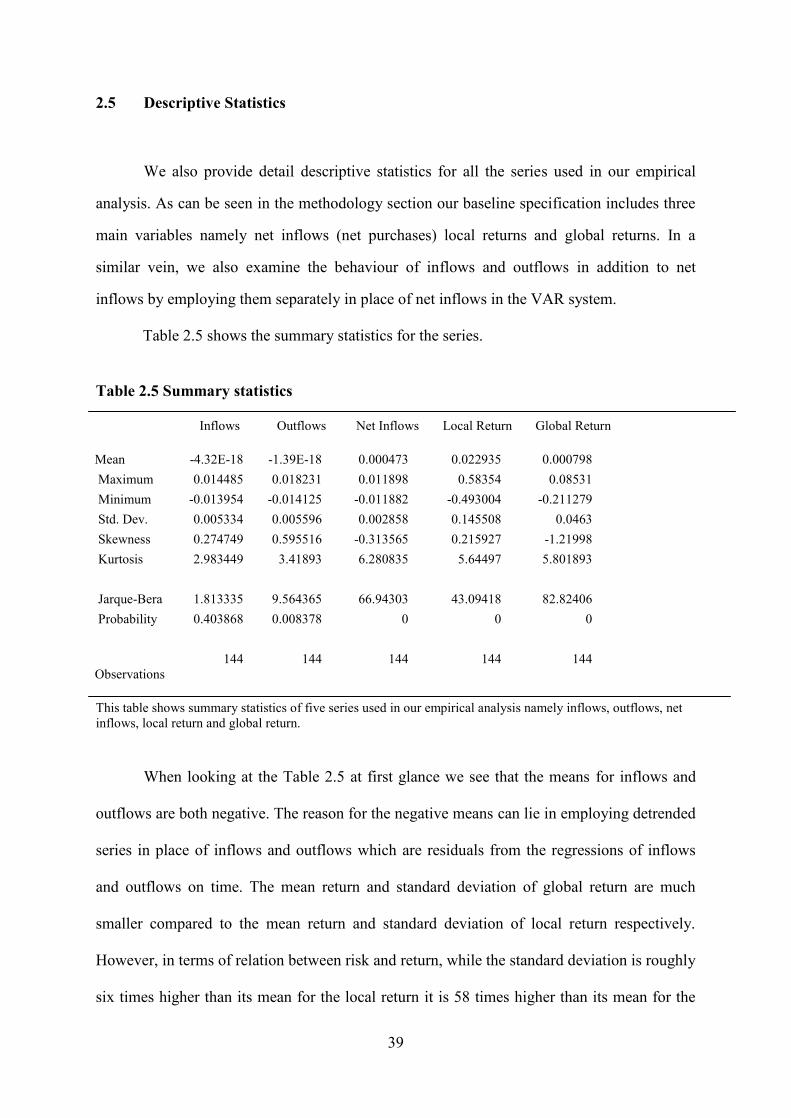
39
2.5 Descriptive Statistics
We also provide detail descriptive statistics for all the series used in our empirical
analysis. As can be seen in the methodology section our baseline specification includes three
main variables namely net inflows (net purchases) local returns and global returns. In a
similar vein, we also examine the behaviour of inflows and outflows in addition to net
inflows by employing them separately in place of net inflows in the VAR system.
Table 2.5 shows the summary statistics for the series.
Table 2.5 Summary statistics
Inflows Outflows Net Inflows Local Return Global Return
Mean -4.32E-18 -1.39E-18 0.000473 0.022935 0.000798Maximum 0.014485 0.018231 0.011898 0.58354 0.08531Minimum -0.013954 -0.014125 -0.011882 -0.493004 -0.211279Std. Dev. 0.005334 0.005596 0.002858 0.145508 0.0463Skewness 0.274749 0.595516 -0.313565 0.215927 -1.21998Kurtosis 2.983449 3.41893 6.280835 5.64497 5.801893
Jarque-Bera 1.813335 9.564365 66.94303 43.09418 82.82406Probability 0.403868 0.008378 0 0 0
Observations144 144 144 144 144
This table shows summary statistics of five series used in our empirical analysis namely inflows, outflows, netinflows, local return and global return.
When looking at the Table 2.5 at first glance we see that the means for inflows and
outflows are both negative. The reason for the negative means can lie in employing detrended
series in place of inflows and outflows which are residuals from the regressions of inflows
and outflows on time. The mean return and standard deviation of global return are much
smaller compared to the mean return and standard deviation of local return respectively.
However, in terms of relation between risk and return, while the standard deviation is roughly
six times higher than its mean for the local return it is 58 times higher than its mean for the

40
global return case. According to the risk-return trade-off, expected return for investing in
global market indices is not high enough to justify its risk compared to the expected return
investing in Istanbul stock market index.
When looking at skewness values, we see that the distributions of net flows and
global return are negatively skewed (left tail heavier than the right tail) while the distributions
of other series are positively skewed (right tail of the distribution is dominant) indicating that
they are non-symmetric, since a distribution that is symmetrical should have a skewness
value of zero or near zero.
In terms of kurtosis, a normal distribution has a kurtosis value of 3. If the kurtosis
value exceeds 3, the distribution is peaked (leptokurtic) relative to the normal; if the kurtosis
value is less than 3 then it indicates a flat (platykurtic) distribution relative to the normal.
When looking at the Table 2.5 we see that apart from inflows and outflows other three series
exhibit high level of kurtosis, which indicates that these series are leptokurtic. The leptokurtic
series is characterised by very frequent medium or large changes than implied by the normal
distribution.
When looking at the Jarque-Bera test statistics, which is used for testing whether the
series is normally distributed, we reject the hypothesis of normal distribution for all series,
except for inflows at the 1% level. However, this is not uncommon in asset returns especially
for high frequency return data. Fama (1965) was among the first to document evidence that
the stock returns are not normally distributed.8
8 The distribution of security returns is assumed to have no effect on t-statistics in the empirical literature due toits asymptotic properties. Lehman (1986) shows that, asymptotically, sample t-statistics are valid regardless ofthe underlying distribution.

41
In addition, as will be seen in the following section, we conduct further robustness
checks to investigate whether our inferences change. For example, we divide our sample into
two parts, with December 2002 being the break point. The earlier part of our sample period is
characterized by persistent macroeconomic and political instability and the later part showed
a significant improvement in stability. Table 2.6 and Table 2.7 show summary statistics of the
series used in the first and second period, respectively.
Table 2.6 Summary statistics in the first period (1997-2002)
Net Inflows Local Return Global Return
Mean -0.000276 0.036327 0.000223Maximum 0.005801 0.58354 0.08531Minimum -0.011882 -0.493004 -0.144471Std. Dev. 0.002764 0.180613 0.049477Skewness -1.104172 0.168379 -0.613888Kurtosis 6.180843 4.444235 2.961972
Jarque-Bera 44.35885 6.506031 4.463775Probability 0 0.038657 0.107326
Observations 71 71 71This table shows summary statistics of three series used in our baseline specification namely net inflows, localreturn and global return.
When looking at the Table 2.6 and Table 2.7 we see that while the mean for inflows is
negative in the first half it appears to be positive in the second half, which confirms a
remarkable increase in foreign investment due to an improvement in stability in Turkey.
Standard deviations of inflows and global return are almost same in both periods, whereas the
standard deviation of local return is lower in the second half possibly reflecting positive
relation between risk and return since local return also appears to be lower compared to first
period.

42
Table 2.7 Summary statistics in the second period (2003-2008)
Net Inflows Local Return Global Return
Mean 0.001201 0.009909 0.001356Maximum 0.011898 0.236478 0.08286Minimum -0.0067 -0.25481 -0.211279Std. Dev. 0.002776 0.099936 0.043324Skewness 0.372042 -0.529817 -2.06692Kurtosis 5.80991 3.403219 10.29489
Jarque-Bera 25.69981 3.909793 213.8415Probability 0.000003 0.141579 0
Observations 73 73 73This table shows summary statistics of three series used in our baseline specification namely net inflows, localreturn and global return.
In terms of skewness, while net inflows and global return are moderately negatively
skewed in the first half we see more pronounced negative skewness for global return in the
second half.
In terms of kurtosis, net inflows are leptokurtic in both periods. Local return is
moderately leptokurtic in the first half, whereas it is not in the second period. While the
kurtosis value of global return is near 3 in the first half it is considerably high (leptokurtic) in
the second period with the value of over than 10.
When looking at the Jarque-Bera test statistics we reject the hypothesis of normal
distribution for inflows in both periods at the 1% level. For local return, while we can reject
the null of normality at the %5 level in the first period we cannot reject it even at the 10%
level in the second half. However, the case is opposite for global return. That is, we cannot
reject the null of normality in the first half, whereas it is strongly rejected in the second
period.

43
Furthermore, as a robustness check, we also partition the data for up and down past
local and global market returns by using dummy variables. Table 2.8 shows summary
statistics of the returns data used in our analysis which are partitioned by the previous
month’s return.
Table 2.8 Summary statistics of returns in Falling and Rising markets
Down Local Markets Up Local Markets Down Global Markets Up Global Markets
-0.042557 0.065492 -0.017001 0.0177990 0.58354 0 0.08531
-0.493004 0 -0.211279 00.078353 0.097057 0.032580 0.021744
-2.919147 2.479285 -2.872492 1.13388413.9866 10.85376 13.28743 3.37888
928.7469 517.6135 833.0158 31.717950 0 0 0
144 144 144 144
This table shows summary statistics of four return series used in our empirical analysis
Since we partition the data for negative and positive values the means and skewness
values for the generated series are of the expected signs as can easily be seen from the Table
2.8. They are either negatively or positively skewed. When looking at the kurtosis values the
case is different for up global markets compared to other three series. While these three series
are pretty leptokurtic the up global markets is not. It has a kurtosis value near 3 which is very
close to normal distribution. As a last, when looking at the Jarque-Bera test statistics we
reject the hypothesis of normal distribution for all series at the 1% level showing that all
series are not normally distributed.
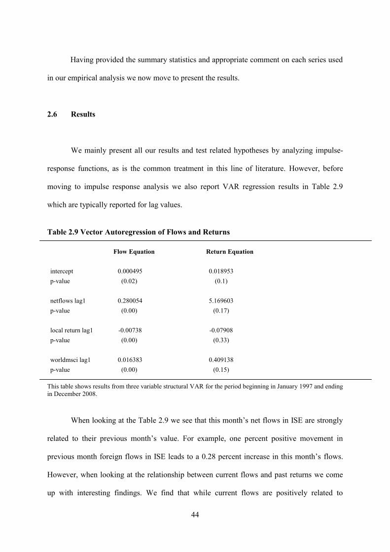
44
Having provided the summary statistics and appropriate comment on each series used
in our empirical analysis we now move to present the results.
2.6 Results
We mainly present all our results and test related hypotheses by analyzing impulse-
response functions, as is the common treatment in this line of literature. However, before
moving to impulse response analysis we also report VAR regression results in Table 2.9
which are typically reported for lag values.
Table 2.9 Vector Autoregression of Flows and Returns
Flow Equation Return Equation
intercept 0.000495 0.018953p-value (0.02) (0.1)
netflows lag1 0.280054 5.169603p-value (0.00) (0.17)
local return lag1 -0.00738 -0.07908p-value (0.00) (0.33)
worldmsci lag1 0.016383 0.409138p-value (0.00) (0.15)
This table shows results from three variable structural VAR for the period beginning in January 1997 and endingin December 2008.
When looking at the Table 2.9 we see that this month’s net flows in ISE are strongly
related to their previous month’s value. For example, one percent positive movement in
previous month foreign flows in ISE leads to a 0.28 percent increase in this month’s flows.
However, when looking at the relationship between current flows and past returns we come
up with interesting findings. We find that while current flows are positively related to

45
previous month’s global returns they are negatively related to previous month’s local return.
In other words, an increase in previous’ months local return leads to a decrease in current
foreign flows.
Table 2.9 also presents the return equation of the VAR which examines the
relationship between current market returns and past foreign flows as well as lagged returns.
When looking at the t-statistics we see that none of lag variables are statistically significant.
Foreign flows are not significant predictors of current returns at lag 1. This result shows that
there is no Granger bi-causality between the two variables. However, there may still be
instantaneous granger causality between the two when there is strong contemporaneous
correlation between net flows and local returns. Table 2.12, in section 2.6.2, shows this fairly
strong contemporaneous correlation between net flows and local returns. What all this means
is that increased net purchases of foreigners lead to a larger price increase, but this impact is
only contemporaneous and transitory as it dies out rather quickly. This issue will also be
analyzed in a more detailed way via impulse response functions in the following section.
Impulse response functions (IRF) show the dynamic behaviour of a variable due to a
shock in another variable in the system. In all IRF graphs to follow, the black line in the
middle represents a point estimation of impulse responses. Since it is not possible to know the
coefficients of the VAR with certainty, computing standard errors for impulse responses is a
common procedure in VAR analysis. Monte Carlo simulation procedure of Sims and Zha
(1999) is used in computing confidence bands for impulse responses. A 90% confidence
interval is constructed with 5000 replications, which is shown by the upper and lower blue
lines. Statistical significance is implied when neither of the confidence bands crosses the x-

46
axis. If, to the contrary, the x-axis falls within the confidence bands then the null hypothesis
that a shock has no effect cannot be rejected.
2.6.1 The response of net flows
2.6.1.1 The Relation of Foreigners’ Trading to Past Local Returns
We test hypothesis one by studying the response of net purchases (normalized by the
total market capitalization) to innovations in domestic returns. Responses of net purchases are
calculated up to five months, and it can easily be seen in Figure 2 that the total effect is
completed within five months. As stated previously, the common assumption is that flows
have contemporaneous effect on domestic returns, but not vice versa, therefore domestic
returns affect equity flows with a lag. This can be seen in the response of net inflows in
period 0.
The cumulative response of net purchases to a one standard deviation innovation in
domestic return is negative. Lag responses are negative and statistically significant up to the
third period. The cumulative response corresponds to -0.1028% of the market capitalization.
The bulk of the effect is observed in the first period with 81.5% of the total effect. For
example, the estimate of –0.0838% for the period 1 in Figure 2 shows that a 10% (0.69 of
monthly standard deviation) price increase of the local market is associated with a decrease
in foreigners’ net purchases by 0.0578% (0.000838*0.69) of the market capitalization in the
subsequent month. Using the market capitalization at the midpoint of our sample period, this
figure would be equivalent to about US$ 231 million.
This estimate can be compared with estimates of earlier papers. Dahlquist and
Robertsson (2004), studying the Swedish market on a monthly basis, report a 0.043%

47
increase in the subsequent month’s net inflows for a similar innovation (10%) in domestic
returns. The response has the opposite sign with respect to our results. Although results of
studies using monthly and daily data should not be directly compared to each other, we can
also mention that Richards (2005) estimates the median cumulative impulse response for six
Asia-Pacific markets to be about 0.0039%, again an opposite sign compared to our results.
Figure 2.2: Impulse Response of Net Inflow to a Shock in Domestic Return
This figure shows impulse response of net inflow to a shock in domestic Return. The vertical axis showsnormalized net purchases (as a percentage of market capitalization per month). The horizontal axis shows timescale which is expressed in months. The black line in the middle represents the impulse responses, and the upperand lower blue lines represent the 90% error bands. The scale corresponds to the normalized net purchases (as aratio of the market capitalization) that would result from a one standard deviation innovation in domestic return.(Full-sample standard deviation of monthly returns is 14.5%.)
Regarding the hypothesis one, the intriguing key difference in our results is that
monthly net purchases are found to be negatively affected by past monthly returns, which
suggests that foreign investors exhibit negative feedback trading in the ISE. This finding from
a different region sheds new light on the issue of whether foreign investors’ pursuing positive
feedback trading strategies is a general phenomenon.
Net
flo
w
Time (month)

48
We are not aware of many studies that have documented significant evidence of
negative feedback trading by foreign investors.9 For example, Stulz (1999), Bekaert et al
(2002), Kim and Wei (2002), and Dahlquist and Robertsson (2004), employing monthly data,
find strong evidence of positive correlation between current foreign flows and lagged local
equity returns.10 Furthermore, Karolyi (2002) who studies Japanese markets using weekly
data also finds evidence consistent with momentum trading among foreign investors during
and after the Asian financial crisis. Choe et al (1999), Froot et al (2001), Griffin et al
(2004),11 and Richards (2005),12 using daily data, also conclude that international investors
are positive feedback traders in these emerging markets.
Our finding is also in striking contrast to most of the available theory. The models of
Brennan and Cao (1997) and Griffin et al (2004) both predict high domestic returns to be
associated with positive net flows. The intuition is that foreign investors are less informed
(this is also a reason for them to exhibit home bias), hence their expectations are more
extrapolative. Brennan and Cao further explain that public news causes larger shifts, which
are correlated with current returns, in foreigners’ expectations. Their model allows for the
possibility of contrarian trading by foreigners only where foreigners have no information
9 One exception may be Swanson and Lin (2003) who, using monthly data from 1988 to 2002, report a negativerelation between net flows and past returns for 4 out of the 8 Asian countries they study. However, that studysuffers from several methodological drawbacks such as using only US flows, not employing VAR methodology,not controlling for global returns, and first-differencing flows rather than normalizing them by marketcapitalization.10 Clark and Berko (1997), using monthly data on Mexico from 1989 to 1996, fails to find any relation betweenflows and past domestic returns. However, this study does not employ VAR methodology, and the specific testdoes not control for global returns.11 The results of Griffin et al. (2004) on Slovenia suggest significant negative feedback trading. While Griffin etal. (2004) questioned the legitimacy of reporting results on Slovenia due to the small size (add partialrestrictions as another concern), we find this result interesting as Slovenia is another EEMENA country withcurrent account deficit.12 Richards’ (2005) results on KSE (Korea) suggest negative feedback trading with respect to domestic return,but not statistically significant at the 10% level. Richards interprets his overall results as evidence of positivefeedback trading. Furthermore, our own analysis using daily data from 2001 to 2009 and the same methodologyas Richards’ suggests significant positive feedback trading in the KSE. Hence, Richards’ finding on KSE wassample-specific and confined to his short (1999-2002) sample period, and Korea is not an exception to positivefeedback trading.

49
disadvantage to begin with, but then domestic investors receive a more precise signal.
However, this is not consistent with our findings, presented later, which suggest that
foreigners’ surprise trades contain some predictive ability. The only theory consistent with
our finding is that of Hau and Rey (2004) who suggest that foreigners take portfolio
rebalancing action following increases of host-market equity prices to bring their portfolio
back into proper relationship (previously stated weight targets). While foreign investors are
trying to bring the portfolio weights into a proper relationship, their trading can appear as if
they pursue contrarian strategy. Note, however, that Hau and Rey’s theory relies on managing
exchange rate exposure and applies to large host markets rather than emerging markets.
Moreover, it is silent on the predictive power of net flows. Another possible explanation for
the negative feedback trading may be foreign investors’ perceptions on valuations. In an
environment where fundamentals are very volatile, informed trading by sophisticated traders
taking advantage of fluctuations associated with extreme sentiment may seem like contrarian
trading. We favour this explanation, which would also be supported by the high standard
deviation of monthly local returns as well as by additional findings presented below.
Moreover, in the light of findings of positive feedback trading with respect to domestic
returns in other markets, portfolio rebalancing does not seem to be the universal explanation.
It must be that foreign investors are able to rationally adjust their trading style according to
specific factors of the country in question. Specifically, the instability of fundamentals or
extreme sentiment trading by domestic investors in Turkey (or perhaps both) may have
rationally led foreigners to pursue contrarian behaviour.
To investigate this possibility further, we divide our sample into two parts, with
December 2002 being the break point. The earlier part of our sample period, shown in Panel
A in figure 2.3, is characterized by persistent macroeconomic and political instability,

50
whereas the later part, shown in Panel B in figure 2.3, showed a significant improvement in
stability. Results suggest that the finding of negative feedback trading is robust (even though
it is not significant after the first subsequent period for the 2003-2008 sample period) in both
subsamples. Further, the negative relation between net flows and past returns is stronger in
the 1997-2002 period as compared to 2003-2008. Given that the standard deviation of
monthly returns fell from 18.2% in the pre-2003 period to 9.6% in the post-2003 period, the
decrease in foreigners’ tendency to negative-feedback trade suggests that foreigners may
rationally be adapting their trading style to the changing degree of stability of the
fundamentals.
We conduct further robustness checks to investigate our finding that seems to suggest
contrarian trading by foreigners. Previous studies except Griffin et al (2004) ignore potential
asymmetries in foreigners’ trading in up and down markets. However, one may argue that if,
for some reason, foreign investors react differently to market’s up movements compared to
down-, then ignoring asymmetries might produce biased coefficients. Therefore, we partition
the data for up and down past market returns by using a dummy variable, and re-run our
impulse-response analysis.
We find that while return shocks in rising markets significantly decrease subsequent
foreign net purchases (as shown in Panel A, Figure 2.4), shocks in falling markets are found
to have no significant effect on foreign investors’ net trading (Panel B). The observed
asymmetry is robust to subsample variation. This observed significant asymmetry warns
against the sensitivity of our results to the sign of past local market return. However, our
finding is again surprising given that most of the existing theories on positive feedback

51
trading would predict a positive relation between lagged returns and foreign inflows,
particularly in rising markets.
Figure 2.3 Impulse Response of Net Inflows to a Shock in Domestic Return in differentsub periods:
Panel A: Response of net flows to a shock in domestic returns in the first period (1997-2002)
Panel B: Response of net flows to a shock in domestic returns in the second period (2003-2008)
This figure shows impulse responses of net inflows to a shock in domestic return in different sub periods. PanelA and Panel B show the response of net flows to a shock in domestic returns in the first (1997-2002) and secondperiod (2003-2008) respectively. The vertical axis shows normalized net purchases (as a percentage of marketcapitalization in each month). The horizontal axis shows time scale which is expressed in months. The black linein the middle represents the impulse responses, and the upper and lower blue lines represent the 90% errorbands.
Net
flo
w
Time (month)
Net
flo
w
Time (month)

52
Further, behavioural theories predict more positive feedback trading when the market
is rising where sentiment traders may dominate than when the market is falling where
fundamentals prevail. Models based on less-informedness of foreigners (Brennan and Cao,
1997; Griffin et al 2004) predict symmetric positive-feedback-trading by foreigners. Hence,
our evidence of contrarian trading only in rising markets contradicts with the view that
foreigners are uninformed and, strictly, that they are more prone to sentiment.
Our interpretation of the asymmetry is as follows: Foreigners take advantage of
excessive bullish sentiment among local traders by selling to them after price increases, while
market falls are generally triggered by bad news symmetrically perceived by two types of
traders rather than by sentiment (we present our anecdotal observations in the final section).13
One possibility is that foreign investors may pursue positive feedback trading over
horizons shorter than the frequency of data in our study, and then become contrarian over
longer horizons exceeding a month. To investigate this possibility, we follow the suggestion
of Warther (1995), which was also implemented by Clark and Berko (1997), and regress
monthly net flows on returns during the last 2 weeks of the month (W2) and those during the
period covering the first two weeks of the current month and last week of the previous month
(W1). Positive feedback trading requires the coefficient of W1 to be greater than the
coefficient of W2. However, results reported in Table 2.10 show just the opposite: The
coefficient of W2 is more than double that of W1. Furthermore, only the coefficient of W2 is
statistically significant. Thus, there is no evidence of positive feedback trading at the weekly
horizon, either. Our result is similar to that of Clark and Berko (1997) on Mexico. The only
possibility for positive feedback trading remains at the daily and intraday horizons.
13 Our inference is symmetrically consistent with the findings from Asia that foreigners acted as liquidityproviders during the crisis in 1997, when sentiment among domestic investors was extremely bearish (see Choeet al., 1999).

53
Table 2.10 Regression of monthly net flows on weekly returns
Variable Coefficient t- statistic
Constant 0.0003 0.91W1 0.0044 1.48W2 0.0111 5.80
This table shows the regression of monthly net flows on weekly returns. W1 denotes the period covering thefirst two weeks of the current month and last week of the previous month. (W2) denotes the period during thelast 2 weeks of the month. The t-values are corrected for heteroskedasticity and autocorrelation with Newey-West procedure.
Figure 2.4 The Differential Response of Net Inflows to a Shock in Domestic Returns inRising and Falling Markets
Panel A Response of net flows to a shock in domestic returns in rising markets
Panel B Response of net flows to a shock in domestic returns in falling markets
This figure shows the differential response of net inflows to a shock in domestic returns in rising and fallingmarkets. Panel A and Panel B show the response of net flows to a shock in domestic returns in rising and fallingmarkets respectively.The vertical axis shows normalized net purchases (as a percentage of market capitalizationin each month). The horizontal axis shows time scale which is expressed in months. The black line in the middlerepresents the impulse responses, and the upper and lower blue lines represent the 90% error bands.
Net
flo
w
Time (month)
Net
flo
w
Time (month)

54
Additionally, as returns relevant to foreign investors are foreign currency
denominated returns, a robustness check with US$ returns is also warranted. Using US$
domestic returns, which can be found in appendix A2.5, we also obtained qualitatively the
same results.
A complementary step is to relate inflows and outflows separately to past returns.
Hence, we repeat the same VAR impulse response analysis using inflows and outflows
normalized by market capitalization, instead of net flows. The resulting impulse response
functions are portrayed in Figure 2.5. Interestingly, both inflows and outflows respond
positively (the former insignificantly) to past return shocks, unlike net flows which respond
negatively. However, as the positive response of outflows is much stronger than inflows, the
net flows exhibit negative correlation with past returns.14
The only study that employs inflows and outflows separately in the VAR framework
is Dahlquist and Robertsson (2004). They find that inflows positively respond to returns,
while outflows do not significantly vary. Hence, both buying and selling behaviour of
foreigners in Sweden differ from that in Turkey. The difference is consistent with the view
that foreigners are able to adjust their trading style rationally according to the stability of
fundamentals. In our case, where the behaviour of net flows suggests negative feedback
trading, the positive response of inflows to past returns suggests that some positive feedback
buyers coexist with informed (or, using more accurate terminology, rational) profit takers. In
other studies where positive feedback trading was reported, a corresponding insight remains
to be specified. Given the result in figure 2.5, a further decomposition of inflows and
14 Another study that relates inflows and outflows separately to past returns is Swanson and Lin (2003). Despitethe methodological imperfections mentioned earlier, they obtain the same findings as we do, thus the discoveryof this pattern should be credited them.

55
outflows in rising and falling markets is warranted. Figure 2.6 shows the VAR impulse-
response results on data partitioned by the previous month’s return.
Panel A suggests that inflows do not respond to the magnitude of positive local
returns, while panel C shows that outflows significantly increase with the magnitude of
positive returns. Panel B implies more (less) inflows following smaller (larger) price
decreases. Panel D similarly implies more (less) outflows following smaller (larger) price
decreases. That is, foreigners tend to buy and sell less following large negative returns, which
is fairly consistent with well-known findings on price-volume relationship (i.e.; volume tends
to shrink following sharp falls). The responses to positive returns, however, suggest that
foreigners, while increasing their sales, do not increase their purchases with positive returns.

56
Figure 2.5 Differential Responses of Inflows and Outflows to a Shock in Local Returns
Panel A: Response of outflows to a shock in local returns
Panel B: Response of inflows to a shock in local returns
This figure shows differential Responses of Inflows and Outflows to a Shock in Local Returns. The vertical axisshows normalized sales and purchases (as a percentage of market capitalization in each month) in Panel A andPanel B respectively. The horizontal axis shows time scale which is expressed in months. Black line in themiddle represents the impulse responses, and the upper and lower blue lines represent the 90% error bands
Ou
tflo
wIn
flo
w
Time (month)
Time (month)

57
Figure 2.6: The Break-Down of Inflows and Outflows in Rising and Falling Markets
A. The Response of Inflows in Rising Markets B. The Response of Inflows in Falling Markets
C. C. The Response of Outflows in Rising Markets D. The response of Outflows in Falling Markets
This figure shows the Break-Down of Inflows and Outflows in Rising and Falling Markets. The vertical axisshows normalized purchases (as a percentage of market capitalization in each month) in Panel A and Panel Band shows normalized sales in Panel C and Panel D. The horizontal axis shows time scale in all panels which isexpressed in months. In all panels, the black line in the middle represents the impulse responses, and the upperand lower blue lines represent the 90% error bands.
2.6.1.2 Responses of net flows to a shock in net flows
All studies in this line of research have included past flows as a main determinant of
current flows. Furthermore, studies such as Froot et al (2001), Griffin et al (2004) and
Richards (2005) also reported high persistency in equity flows to emerging markets.
Therefore, we also show the graph of the impulse responses function of net flows to a shock
Infl
ow
s
Infl
ow
sTime (month) Time (month)
Ou
tflo
ws
Ou
tflo
ws
Time (month) Time (month)

58
in net flows in figure 2.7, which is estimated from the VAR model described previously, to
better understand the dynamic nature of equity flows. The figure shows that the cumulative
response of net flows to a one standard deviation innovation in net flows is positive. All lag
responses are positive, however statistically significant only for the first period. A 1% shock
in net flows (equivalent to 3.51 standard deviations) corresponds to a cumulative response of
0.95%. 76% of the total effect is observed in the first period. Since the sign of the lag
responses do not change, we find persistence in net flows. However, the persistence we
observe in ISE is short-lived compared to Dahlquist and Robertsson (2004) who report high
persistence in equity flows in Sweden.15 One explanation of the difference may be the
instability of fundamentals in Turkey. Another possibility is that, in some other markets,
persistence could be overestimated due to liberalization effects. Turkey liberalized its equity
market in August 1989 and our data set starts in January 1997. Therefore, our analysis is not
blurred by the initial impact of liberalization (i.e. one-time portfolio rebalancing by
international investors) as documented in Bekaert et al (2002) and Dahlquist and Robertsson
(2004).
2.6.1.3 Responses of net flows to a shock in global returns
We also look at the responses of net flows to a shock in global return due to two
reasons. First, as mentioned in Griffin et al (2004) foreign investors might invest more in
emerging stocks following increases in their home markets due to portfolio rebalancing
effects. Second, foreigners might extract information from global returns about prospects for
emerging markets (Richards, 2005). Now when we move to the responses of net flows which
are shown in figure 2.8 we see that the response at the first and second lags are significantly
15 Froot et al. (2001) and Richards (2005) also report high persistence, however as they use daily data, theirfindings are not directly comparable to ours.

59
positive (marginally so at the second lag), and insignificant thereafter. Thus, foreigners’
responses to global returns are strikingly different from that to domestic returns. Specifically,
they do exhibit positive feedback trading with respect to global returns. Our result is
consistent with Richards (2005). Positive feedback trading with respect to global returns may
be consistent with portfolio rebalancing or a belief in spill-over effects from the global
economy.
The evidence that foreigners respond in different ways to past domestic and global
returns, at the same time in the same market, is noteworthy. Specific characteristics of the
Turkish economy, mentioned previously, may have led foreigners to suspect the
sustainability of positive domestic returns and thus to respond to domestic factors differently.
Figure 2.7: Impulse Response of Net flows to a Shock in Net Inflow
This figure shows the impulse response of net inflow to a shock in net inflow. The vertical axis showsnormalized net purchases (as a percentage of market capitalization). The horizontal axis shows time scale inmonths. The impulse-response is shown with 90% confidence intervals derived from a Monte Carlo simulation.Note that the number at period 0 is just the standard deviation of net flows.
Net
flo
ws
Time (month)

60
A partitioning in rising and falling global markets portrayed in Figure 2.9 below
suggests another interesting asymmetry. The responses to positive global returns
(significantly positive in the contemporaneous period) becomes negative at lags 2 and 3 in
rising global markets. However, it remains significantly positive at lags 1 and 2, in the case of
falling global markets. This suggests positive feedback trading in falling markets, but not in
rising markets (in contrast, some profit taking tendency). This is a new finding which is not
consistent with behavioural (sentiment) theories that predict more positive feedback trading
following price increases.
Figure 2.8: Response of net flows to a shock in global return
This figure shows response of net flows to a shock in global return The vertical axis shows normalized netpurchases (as a percentage of market capitalization). The horizontal axis shows time scale in months. Theimpulse-response is shown with 90% confidence intervals derived from a Monte Carlo simulation.
Net
flo
ws
Time (month)

61
Figure 2.9 The Differential Response of Net Flows to a Positive Shock in Global Returnin Rising and Falling Global Markets
Panel A: Impulse Responses in Rising Global Markets Panel B: Impulses Response in Falling Global Markets
This figure shows responses of net flows to a positive shock in global return in rising and in falling globalmarkets. Panel A and Panel B show Impulse Responses of net flows in Rising and falling Global Marketsrespectively. The vertical axis shows normalized net purchases (as a percentage of market capitalization in eachmonth). The horizontal axis shows time scale which is expressed in months. The black line in the middlerepresents the impulse responses, and the upper and lower blue lines represent the 90% error bands.
2.6.1.4 Variance Decomposition
The system dynamics can also be traced with a decomposition of forecast error
variance for the net inflows into its own, domestic and global return shocks in the VAR
model. Results in Table 2.10 suggest that at the one month horizon 7.6% of the forecast error
variance can be traced to innovations in global return. At the two month horizon, the
proportion that can be traced to domestic returns is 8.35%, while the proportion traced to
global returns decreases only slightly. At the three months horizon, the proportion due to
shocks in local returns increases to 8.74%. The proportions remain fairly stable thereafter.
Our results with this method indicate that local returns account for a slightly larger proportion
of the forecast error variance in net flows than global returns do. We are aware of only two
studies reporting variance decomposition results: Karolyi’s (2002) results on Japan are not
Net
flo
ws
Net
flo
ws
Time (month) Time (month)

62
comparable to ours as he does not include global returns. Richards (2005), using daily data,
finds that, as the median value for six Pacific markets, domestic (US) returns account for
3.3% (6.1%) of the variance in net inflows. In 3 cases (Indonesia, Philippines and Thailand)
domestic returns are more important, while in Taiwan and Korea (KSE) US returns are
dramatically more important. In our sample, the portion of the variance accounted for by
domestic returns is higher compared to the median of 6 Asia-Pacific markets.
Apart from this, regression analysis suggests that 33.4% of the total variation in net
flows can be accounted for by these 3 variables, and 26.7% of it can be predicted using
variables known at the end of the previous period. Hence, a nontrivial portion of variation in
net foreign flows is predictable using past local and global returns and past flows.
Table 2.11: Decomposition of forecast error variance for the net flow
Forecast Horizon Std Error Global Return Net Flow Local Return---------------------------------------------------------------------------------------------------------------------------------------
1 0.00258 7.60 92.4 0.002 0.00277 7.52 84.13 8.343 0.00278 7.48 83.78 8.744 0.00278 7.48 83.77 8.755 0.00278 7.48 83.77 8.756 0.00278 7.48 83.77 8.757 0.00278 7.48 83.77 8.758 0.00278 7.48 83.77 8.759 0.00278 7.48 83.77 8.75
10 0.00278 7.48 83.77 8.75___________________________________________________________________________The table provides the decomposition of forecast error variance in net flows due to shocks in each of thevariables in the system. Forecast horizon refers to the number of months. Forecast horizon 1 corresponds to thecontemporaneous month. The second column in the table shows the standard error of the forecast for netinflows. The remaining three columns show the percentage of the variance of the error made in forecasting netflows due to a specific shock (i.e. error term in global return, net flow, and local market return equations,respectively) at a given horizon. Numbers in each row add up to 100%. The figure for local returns at forecasthorizon 1 is 0 by ordering assumption.

63
2.6.2 The Impact of Foreigners’ Trading on Domestic Equity Prices
In this section we test whether foreigners’ net purchases increase equity prices.
Conditional on the statistical significance, we provide an estimate of the magnitude of price
impact of foreigners’ net purchases, and also find out whether this price impact is temporary
or permanent. The analysis starts with a simple bivariate regression of domestic returns on
net inflows (seen in the first panel in Table 2.11) showing fairly strong contemporaneous
correlation between net flows and local returns, with a t-statistic of 5.27. However, as net
flows are significantly positively related to global returns (t=5.00, R2=12.7%, univariate
regression of net flows on global returns not reported in the table), most of this
contemporaneous relationship is due to the positive relation between net flows and global
returns. When our exogenous variable, global returns, is included, the R2 of the return
equation increases substantially from 16.4 to 32.9% percent (second panel in Table 2.11).
The significance of the coefficient on net flows decreases only slightly, which shows that net
purchases still remain a significant determinant of local returns.
We also decompose the net inflows into expected and unexpected components,
following other papers such as Richards (2005), to compare their effects on local returns. The
third panel shows regression of domestic returns on a constant, unexpected flows, expected
flows, and the exogenous control variable. While the coefficient on unexpected net flows is
found to be significant the expected net flows is not. This is consistent with Warther’s (1995)
argument and Richards’ (2005) results in five of six Pacific emerging markets.

64
Table 2.12 The price impact of the net purchases of foreign investors
Regression of domestic returns on a constant and net flows (with t statistics in parantheses)
Coefficient on net flows: 20.64 R2 = 16.4%(3.63)
Regression of domestic returns on a constant, net flows, and control variable (MSCI world index returns)
Coefficient on net flows: 12.82 R2 = 32.9%(2.38) R2 with only MSCI-world return = 27.3%
Coefficient on MSCI-world return: 1.36(4.7)
Regression of domestic returns on a constant, unexpected flow,expected flow, and control variable (MSCI worldindex returns)
Coefficient on unexpected flows: 12.45 R2 = 34.5%(3.18)
Coefficient on expected flows: 13.06(1.59)
Coefficient on MSCI-world return: 1.35(6.06)
Number of Observations: 143
The first panel shows the results of regression of monthly returns in ISE on only a constant and net inflows. Theregression in the second panel includes the control variable, broad market returns. The regression in the thirdpanel decomposes net inflows into expected and unexpected flows, with expected flows defined as the fittedvalue from the bivariate-VAR described previously, including only those variables pre-determined at the end ofthe previous domestic trading month. t-statistics are shown in parentheses. Domestic return is defined as thereturns of the ISE all-share-index.
In testing the hypothesis two the relevant impulse response function is the response of
domestic returns to innovations in net flows, which is estimated from the SVAR model
described previously and illustrated in Figure 2.10. Estimation is based on the same
identification assumptions as before.
The contemporaneous and lag responses and the cumulative impact are positive.
Regarding the hypothesis two, foreigners’ net purchases are found to increase equity prices
since instantaneous and lag responses up to the second lag are statistically significant. The
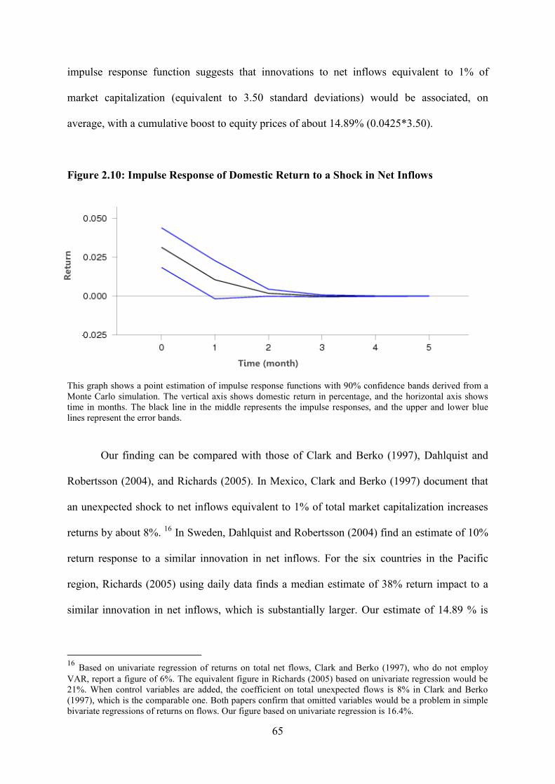
65
impulse response function suggests that innovations to net inflows equivalent to 1% of
market capitalization (equivalent to 3.50 standard deviations) would be associated, on
average, with a cumulative boost to equity prices of about 14.89% (0.0425*3.50).
Figure 2.10: Impulse Response of Domestic Return to a Shock in Net Inflows
This graph shows a point estimation of impulse response functions with 90% confidence bands derived from aMonte Carlo simulation. The vertical axis shows domestic return in percentage, and the horizontal axis showstime in months. The black line in the middle represents the impulse responses, and the upper and lower bluelines represent the error bands.
Our finding can be compared with those of Clark and Berko (1997), Dahlquist and
Robertsson (2004), and Richards (2005). In Mexico, Clark and Berko (1997) document that
an unexpected shock to net inflows equivalent to 1% of total market capitalization increases
returns by about 8%. 16 In Sweden, Dahlquist and Robertsson (2004) find an estimate of 10%
return response to a similar innovation in net inflows. For the six countries in the Pacific
region, Richards (2005) using daily data finds a median estimate of 38% return impact to a
similar innovation in net inflows, which is substantially larger. Our estimate of 14.89 % is
16 Based on univariate regression of returns on total net flows, Clark and Berko (1997), who do not employVAR, report a figure of 6%. The equivalent figure in Richards (2005) based on univariate regression would be21%. When control variables are added, the coefficient on total unexpected flows is 8% in Clark and Berko(1997), which is the comparable one. Both papers confirm that omitted variables would be a problem in simplebivariate regressions of returns on flows. Our figure based on univariate regression is 16.4%.
Ret
urn
Time (month)

66
higher than that of those two using monthly data (which should not be directly compared with
Richards (2005) who employs daily data).17
Having documented the statistical significance of the price impact we now test,
hypothesis three, whether net inflows have a long-lived (permanent) effect on prices or a
temporary effect consistent with the price pressure hypothesis. The price pressure hypothesis
suggests a negative relation between the current inflows and subsequent returns which
implies that net inflows exert temporary contemporaneous pressure on equity prices, and
subsequent returns exhibit reversals as prices return to their fundamental values. The
alternative is that the contemporaneous effect is not reversed over time, consistent with the
information hypothesis and/or the base broadening hypothesis. To display the response of
returns to a shock in net flows more precisely, we present impulse responses calculated up to
nine months in Table 2.12. The price effect dies out quite quickly as the largest effect is
observed in the instantaneous period with a positive sign (72% of the total effect). The total
effect is completed within eight months but it can easily be seen that practically the bulk of
the impact is completed within three months. There are no significant negative lags; in other
words, prices are not observed to return to their previous levels. Therefore, regarding the
hypothesis three, we find no evidence to support the price pressure hypothesis. On the
contrary, our findings support a permanent effect of net flows on stock prices, which can
represent a decrease in the cost of capital as suggested by Bekaert et al (2002) and Dahlquist
and Robertsson (2004). Given the evidence presented in the next section, our results are
consistent with both the base-broadening and information hypotheses.
17 Richards (2005) discusses the reasonableness of his much larger estimates in detail (p.24-25). However, amajor source of difference could be the frequency of analysis, and it is interesting to note that Richards did notmention this. It may be that net flows exhibit negative serial correlation at some lags within a month, so thatprice impacts during the month may cancel out to produce a lower estimate of the contemporaneous priceimpact with monthly data.

67
Table 2.12: Response of domestic return to a shock in net flows
Period Domestic return
0 0.030535131 0.010298742 0.001581453 0.000153144 0.000005495 -0.000001356 -0.000000367 -0.000000058 -0.00000000
First column shows periods in months. Second column shows the point estimates of the impulse responsecoefficients of domestic return portrayed in Figure 2.10. The immediate response of domestic return is seen inperiod 0. As previously mentioned, a common assumption is that flows have contemporaneous effect ondomestic returns but not vice versa.
2.6.3 Foreigners’ Trading in Individual Stocks
The results presented in Table 2.12 and Figure 2.10 also imply statistical evidence of
predictive ability of a modest degree, as shocks to foreigners’ net purchases are followed by
positive returns in the two subsequent periods at borderline levels of significance. This
suggests that net inflows reveal or contain information about future equity prices. However, if
foreigners have private domestic information, it should manifest itself in the stock selection
ability in addition to market-wide timing. Hence, a useful complement of our analysis would
be an assessment of relative performance of stocks which foreigners have most bought or
sold. For this purpose, we use monthly data of net purchases by foreigners in individual
stocks. We include 36 most active (in terms of trading volume) stocks in our analysis.
First, we implement a version of the buy difference methodology, introduced by
Grinblatt and Keloharju (2000) and also implemented by Dahlquist and Robertsson (2004),
which involves computing foreigners’ net buy differences in winning vs. losing stocks for

68
each month. Specifically, for each month, we subtract foreigners’ net buys in the 5 most
losing stocks from their net buys in the 5 most gaining stocks, which gives the “net buy
difference” for the particular month. A positive net buy difference implies that foreigners
bought winners more than losers. In this way, we calculate foreigners’ net buy difference, in
past, current and future months, of the top and bottom performers. Positive buy differences in
previous months imply superior stock selection ability, while positive buy differences in
future months imply positive feedback trading.
The results can be seen in Table 2.13. The significantly positive buy difference in
month 0 confirms the contemporaneous price impact on an individual stock basis. However,
regarding the hypothesis four, the absence of significantly positive buy differences at lags -5
to -1 (at leads 1 to 3) implies no stock selection ability (no positive feedback trading). In
particular, the negative buy differences at months from -1 through -4 suggest that foreigners
were not able to forecast future months’ extreme performers. The positive number in month 1
suggests some small degree of momentum trading, however the negative numbers in months
2 and 3 are consistent with our previous market-wide finding of contrarian trading. It is also
interesting to note that evidence of contrarian trading has weakened in the post-2003
subsample, as was the case with the market-wide results.
These results can be compared to those of Dahlquist and Robertsson (2004), who
obtain significant positive figures in contemporaneous and previous month’s return, which
suggests momentum trading in cross-sectional sense, and numbers close to zero in preceding
months which is consistent with no evidence of informed trading. Our results suggest poorer
performance; the tendency of momentum trading in month 1 is much weaker; and our finding
of contrarian trading in months 2 and 3 is again unique.

69
Table 2.13: Net buy differences of foreigners
Full Sample 1997-2002 2003-2008
Lead/Lag Avg.Net Buy Diff t-value Avg Net Buy Diff Avg Net Buy Diff
-5 0.0028 0.83 0.0096 -0.0029-4 -0.0027 -0.77 -0.0067 0.0007-3 -0.0048 -1.59 -0.0021 -0.0071-2 -0.0010 -0.29 0.0023 -0.0038-1 -0.0051 -1.42 -0.0060 -0.00420 0.0590 12.58*** 0.0488 0.06831 0.0039 1.01 0.0025 0.00532 -0.0070 -1.82 -0.0106 -0.00373 -0.0031 -0.81 -0.0072 0.0008
Stocks are ranked in terms of their return in month 0, and top and bottom 15% quintiles are identified. Thenumbers represent the difference of foreigners’ net buys in the top quintile minus net buys in the bottom quintilein each of the months from -5 through +3, averaged over the sample period. The t-value corresponds to the testof the null hypothesis that the mean of the net buy difference is 0. The two columns on the right show sub-sample results. *,**,*** denote significance at the 10%, 5% and 1% level respectively.
Then, we revert to our VAR model using relative net flows and relative (abnormal)
returns. As mentioned before the buy ratio difference methodology is not sufficiently
informative. Many studies find a stronger predictive ability of surprise net buys, which
cannot be singled out under the net buy difference methodology. On this basis, our VAR
approach is much more informative. Therefore, a comparison of results under both
methodologies enables us to assess whether failure to employ surprise net buys makes a
significant difference. The estimation results of this VAR model are presented in Table 2.14
which shows impulse responses of returns to past net flows. The first column shows 36 most
active stocks (in terms of trading volume) in the ISE. Other two columns show the impulse
response coefficients of related stock returns for the first and second lags. The results in Panel
A suggest little evidence of predictive ability on the part of foreigners, as there are very few
significantly positive coefficients. In only 6 out of 35 stocks foreigners net purchases are
found to predict next month returns. Thus, the inference on predictive ability under VAR

70
methodology is not much different from that under the net buy difference methodology. In
other words, the surprise component does not have significantly different predictive content.
In addition, Table 2.15 Shows that predictive performance does not vary with the size
of the firm, as t-values reported in Table 2.15 are not significantly correlated with market
capitalization. Overall, regarding the hypothesis four, results in this section suggest that
foreigners do not have private information concerning individual stocks in the ISE.
Table 2.15 Regression of t-statistics on market capitalization
Variable Coefficient t- statistic
Constant 0.923 6.7Market cap -0.009 -0.7
This table shows regression of t-statistics on market capitalization for 36 firms.

71
Table 2.14: Impulse responses in individual stock VAR’s using relative net flows andabnormal returns
LAG1 LAG2STOCKS Coefficient st error t-stat Coefficient st error t-stat
AEFES -0.00803 0.01340 -0.60 0.00176 0.00651 0.27AKBNK -0.00533 0.01653 -0.32 0.00160 0.00157 1.02AKGRT -0.00362 0.01804 -0.20 0.00033 0.00118 0.28ALARK -0.01634 0.01805 -0.91 -0.00057 0.00259 -0.22ARCLK -0.03188 0.01819 -1.75* 0.00446 0.00513 0.87ANSGR -0.02470 0.01783 -1.39 0.00315 0.00382 0.82AYGAZ 0.00009 0.01565 0.01 0.00006 0.00103 0.06BAGFS -0.03985 0.01823 -2.19** -0.00168 0.00509 -0.33DOHOL 0.03668 0.02134 1.72* 0.00749 0.00606 1.24DYHOL 0.04573 0.02311 1.98** 0.00448 0.00676 0.66ECILC -0.00300 0.01946 -0.15 -0.00011 0.00152 -0.07ENKAI -0.02135 0.01642 -1.30 0.00053 0.00275 0.19EREGL -0.00994 0.01731 -0.57 -0.00204 0.00330 -0.62GARAN -0.00205 0.01936 -0.11 -0.00049 0.00241 -0.20GUBRF -0.00869 0.02326 -0.37 0.00015 0.00128 0.12HURGZ -0.00320 0.02215 -0.14 0.00064 0.00188 0.34IHLAS 0.02778 0.02205 1.26 0.00509 0.00518 0.98ISCTR 0.01955 0.01834 1.07 -0.00123 0.00278 -0.44KCHOL -0.02353 0.01777 -1.32 0.00386 0.00430 0.90KRDMD -0.01310 0.02659 -0.49 -0.00754 0.00993 -0.76MIGRS -0.00007 0.01304 -0.01 0.00009 0.00065 0.14NTHOL 0.03746 0.02333 1.61 0.01219 0.00878 1.39PETKM 0.01155 0.01862 0.62 0.00297 0.00410 0.72PTOFS -0.01346 0.01925 -0.70 0.00280 0.00486 0.58SAHOL -0.00383 0.01713 -0.22 0.00057 0.00291 0.19SISE -0.01492 0.01752 -0.85 -0.00325 0.00406 -0.80SKBNK 0.01044 0.02174 0.48 0.00230 0.00456 0.50TCELL 0.04491 0.02070 2.17** -0.00861 0.00786 -1.10THYAO 0.00875 0.01880 0.47 -0.00169 0.00373 -0.45TOASO -0.00713 0.01898 -0.38 -0.00077 0.00238 -0.32TRKCM 0.01527 0.01589 0.96 0.00367 0.00460 0.80TSKB -0.04163 0.02001 -2.08** -0.00033 0.00557 -0.06TUPRS -0.01422 0.01674 -0.85 0.00183 0.00252 0.73ULKER 0.01908 0.01941 0.98 0.00499 0.00739 0.68VESTL -0.00850 0.01685 -0.50 0.00102 0.00154 0.66YKBNK 0.00924 0.02094 0.44 -0.00001 0.00159 -0.01
This table shows impulse responses of returns to past net flows. The first column shows 36 most active stocks(in terms of trading volume) in the ISE. Other two columns show the impulse response coefficients of relatedstock returns for the first and second lags.

72
2.7 Conclusion
The previous empirical work on the joint dynamics of foreign flows and stock market
returns surprisingly neglects the EEMENA region where economies most dependent on
foreign investment inflows are located. Therefore, the results of this study on the ISE, the
largest market in the EEMENA region, are likely to make a key contribution to whether the
findings of extant studies can be generalized into an empirical characterization of the
interaction between foreign investors’ trading and emerging stock market returns. Extant
empirical evidence in this field has so far suggested that foreign investors are positive
feedback traders, which has been used as a justification for the argument that foreign
portfolio flows may destabilize local markets. Our findings suggest that foreigners are
negative feedback (contrarian) traders in the ISE. This is in stark contrast with previous
empirical results and most of the existing theories that previously seemed consistent with
empirical evidence.
The finding of negative feedback trading is robust to sub-sample variation, though we
observe a moderation in the degree of contrarian behaviour post 2003. As stability in
economic and financial conditions has significantly improved since 2003 in Turkey, our
interpretation is that extremely volatile economic conditions dictated negative feedback
trading especially before 2003, and that foreigners as a group are sufficiently sophisticated to
alter their style in line with the changing degree of stability in fundamentals. The same
foreigners over the same sample period exhibit positive feedback trading with respect to past
global returns, which, unlike domestic returns, exhibit persistence. Hence, foreign investors

73
seem to be able to rationally adjust their trading style rather than naively pursuing a specific
feedback trading strategy.
Our intriguing finding motivated us to perform a full exploration: Contrarian trading
is asymmetrically driven by up-markets only. Our interpretation of this new finding is that
foreign investors take advantage of extreme bullish sentiment among domestic investors. This
interpretation is also supported by the fact that the post-2003 period, when the tendency of
negative feedback trading by foreigners moderated, is characterized by less participation by
domestic individual investors. Both inflows and outflows respond positively to past local
returns, while net flows respond negatively, because outflows increase much more than
inflows do following positive returns. This suggests that the group of foreigners may include
some positive feedback buyers, while the majority acts as contrarian profit takers.
We estimate the price impact of foreign net flows as higher than that for Mexico and
Sweden at a monthly frequency. We confirm that the impact of surprise flows is more
significant than that of expected flows. We find no evidence that prices return to their
previous levels. Therefore, our findings do not support the price pressure hypothesis, instead
the price impact is permanent which supports the base-broadening and information
hypotheses. We find statistically borderline-significant evidence of the predictive ability of
net foreign flows. However, the analysis on individual stocks suggests no evidence of
informed trading. Hence, foreigners seem to have no particular advantage in domestic
information, yet their advantage in analyzing push factors and their sophistication lend them
predictive ability with respect to local market returns.

74
Our anecdotal observations around significant information events are particularly
consistent with sophisticated timing. For example, in 1999, significant foreign inflows
preceded the IMF agreement and the launch of EU full membership process in December,
after which domestic investors became extremely optimistic and foreigners heavily sold into
this exaggerated bullish sentiment in early 2000. This was, of course, followed by the
banking crisis in November 2000.
In sum, we show that previous findings that foreign investors are positive feedback
traders may not necessarily be a general phenomenon. Rather, they can rationally adopt a
contrarian style if market conditions justify it. By doing so, they may curb extreme sentiment
fluctuations among domestic investors. This raises serious doubts about the previously
widespread stereo-typing of foreigners as uninformed positive feedback traders and the
justifiability of policies to restrict their trading (including the so-called “smart restrictions”).
The comprehensive exploration presented in this study challenges some previously
well established findings towards a general characterization of foreign investors’ trading
behaviour. Since this study is so far the only major analysis of this type from the EEMENA
region which, in contrast to many Asian markets or Sweden, is highly dependent on foreign
inflows, several intriguing questions arise: Is foreigners’ negative feedback trading confined
to Turkey or common to all high external deficit economies in the EEMENA region? That is,
is it driven by unique characteristics of Turkey such as a high degree of instability and local
investors being excessively vulnerable to bullish sentiment, or solely by large external
deficits? Answers to these questions in order to reach a generalized theory of the interaction
between foreigners’ trading and returns in emerging markets and more appropriate policy

75
guidelines with regard to regulation of foreign portfolio flows (“hot money”) are left to future
studies on more EEMENA emerging markets.
Appendix A2
A2.1 VAR lag order selection
Below is the table that shows suggested lag lengths by various information criteria.
Table A2.1 VAR lag order selection criteria
Lag LOGL LR FPE SIC HQ
0 684.8784 NA 1.49E-07 -9.999496* -10.024921 694.0535 17.9454* 1.38E-07* -9.989935 -10.06622*2 694.4465 0.756976 1.46E-07 -9.851223 -9.9783583 698.3142 7.337409 1.46E-07 -9.763613 -9.9416014 699.3123 1.864035 1.53E-07 -9.6338 -9.8626425 700.8925 2.904742 1.58E-07 -9.512548 -9.7922446 701.8778 1.782206 1.66E-07 -9.382548 -9.7130977 703.5343 2.94761 1.71E-07 -9.262418 -9.6438218 704.9146 2.415609 1.78E-07 -9.138228 -9.570484
This table shows the VAR lag order suggested by information criteria. LOGL and LR denote loglikelihood andsequential modified likelihood ratio test respectively. FPE denote final prediction error. AIC and HQ denoteAkaike information criteria and Hannan-Quinn information criteria respectively. * indicates lag order selectioncriterion.
A2.2 VAR residual portmanteau tests for autocorrelation
Below is the portmanteau test applied to VAR residuals up to 12 lags to see whether
there is evidence of autocorrelation.
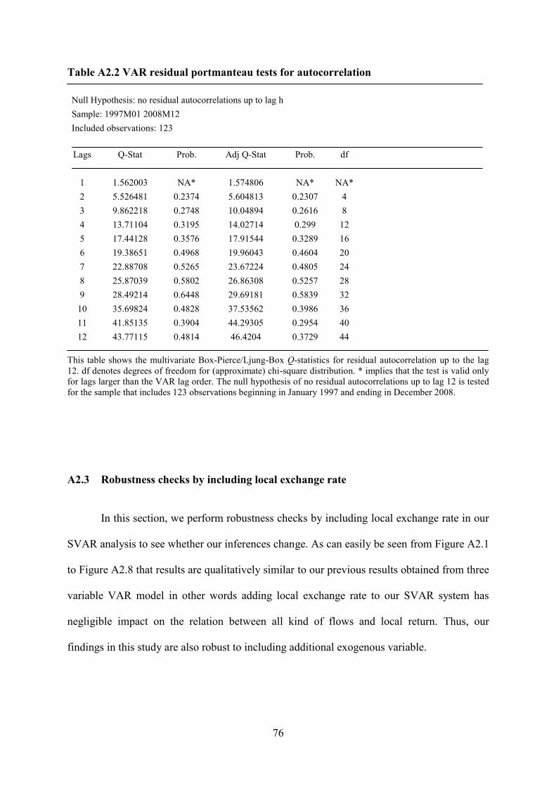
76
Table A2.2 VAR residual portmanteau tests for autocorrelation
Null Hypothesis: no residual autocorrelations up to lag hSample: 1997M01 2008M12Included observations: 123
Lags Q-Stat Prob. Adj Q-Stat Prob. df
1 1.562003 NA* 1.574806 NA* NA*2 5.526481 0.2374 5.604813 0.2307 43 9.862218 0.2748 10.04894 0.2616 84 13.71104 0.3195 14.02714 0.299 125 17.44128 0.3576 17.91544 0.3289 166 19.38651 0.4968 19.96043 0.4604 207 22.88708 0.5265 23.67224 0.4805 248 25.87039 0.5802 26.86308 0.5257 289 28.49214 0.6448 29.69181 0.5839 32
10 35.69824 0.4828 37.53562 0.3986 3611 41.85135 0.3904 44.29305 0.2954 4012 43.77115 0.4814 46.4204 0.3729 44
This table shows the multivariate Box-Pierce/Ljung-Box Q-statistics for residual autocorrelation up to the lag12. df denotes degrees of freedom for (approximate) chi-square distribution. * implies that the test is valid onlyfor lags larger than the VAR lag order. The null hypothesis of no residual autocorrelations up to lag 12 is testedfor the sample that includes 123 observations beginning in January 1997 and ending in December 2008.
A2.3 Robustness checks by including local exchange rate
In this section, we perform robustness checks by including local exchange rate in our
SVAR analysis to see whether our inferences change. As can easily be seen from Figure A2.1
to Figure A2.8 that results are qualitatively similar to our previous results obtained from three
variable VAR model in other words adding local exchange rate to our SVAR system has
negligible impact on the relation between all kind of flows and local return. Thus, our
findings in this study are also robust to including additional exogenous variable.

77
Figure A2.1 Impulse Response of Net Inflows to a Shock in Domestic Returns
The vertical axis shows normalized net purchases (as a percentage of market capitalization per month). Thehorizontal axis shows time scale which is expressed in months. The black line in the middle represents theimpulse responses, and the upper and lower blue lines represent the 90% error bands. The scale corresponds tothe normalized net purchases (as a ratio of the market capitalization) that would result from a one standarddeviation innovation in domestic return. (Full-sample standard deviation of monthly returns is 14.5%.)
Net
flo
ws
Time (month)

78
Figure A2.2 The Differential Response of Net Inflows to a Shock in Domestic Returns inRising and falling markets
A: Response of net flows to a shock in domestic returns in rising markets
B: Response of net flows to a shock in domestic returns in falling markets
This figure shows impulse response of net inflows to a shock in domestic return in different sub periods. PanelA and Panel B show the response of net flows to a shock in domestic returns in the first (1997-2002) and secondperiod (2003-2008) respectively. The vertical axis shows normalized net purchases (as a percentage of marketcapitalization in each month). The horizontal axis shows time scale which is expressed in months. The black linein the middle represents the impulse responses, and the upper and lower blue lines represent the 90% errorbands.
Net
flo
ws
Time (month)
Net
flo
ws
Time (month)

79
Figure A2.3 Differential Responses of Inflows and Outflows to a Shock in Local Returns
A: Response of outflows to a shock in local returns
B: Response of inflows to a shock in local returns
This figure shows differential Responses of Inflows and Outflows to a Shock in Local Returns. The vertical axisshows normalized sales and purchases (as a percentage of market capitalization in each month) in Panel A andPanel B respectively. The horizontal axis shows time scale which is expressed in months. Black line in themiddle represents the impulse responses, and the upper and lower blue lines represent the 90% error bands
Ou
tflo
ws
Time (month)
Infl
ow
s
Time (month)

80
Figure A2.4 The Break-Down of Inflows and Outflows in Rising and Falling Markets
A. The Response of Inflows in Rising Markets B. The Response of Inflows in FallingMarkets
C. The Response of Outflows in Rising Markets D. The response of Outflows in FallingMarkets
This figure shows the Break-Down of Inflows and Outflows in Rising and Falling Markets. The vertical axisshows normalized purchases (as a percentage of market capitalization in each month) in Panel A and Panel Band shows normalized sales in Panel C and Panel D. The horizontal axis shows time scale in all panels which isexpressed in months. In all panels, the black line in the middle represents the impulse responses, and the upperand lower blue lines represent the 90% error bands.
Infl
ow
s
Infl
ow
sTime (month) Time (month)
Ou
tflo
ws
Ou
tflo
ws
Time (month) Time (month)

81
Figure A2.5 Impulse Response of Net Flows to a Shock in Net Flows
This figure shows impulse response of net flows to a shock in net flows. The vertical axis shows normalized netpurchases (as a percentage of market capitalization). The horizontal axis shows time scale in months. Theimpulse-response is shown with 90% confidence intervals derived from a Monte Carlo simulation. Note that thenumber at period 0 is just the standard deviation of net flows.
FigureA2.6 Response of net flows to a shock in global returns
This figure shows response of net flows to a shock in global return The vertical axis shows normalized netpurchases (as a percentage of market capitalization). The horizontal axis shows time scale in months. Theimpulse-response is shown with 90% confidence intervals derived from a Monte Carlo simulation.
Net
flo
ws
Time (month)
Net
flo
ws
Time (month)

82
Figure A2.7 The Differential Response of Net Flows to a Positive Shock in GlobalReturns in Rising and Falling Global Markets
Panel A: Impulse Response in Rising Global Markets
Panel B: Impulse Response in Falling Global Markets
This figure shows responses of net flows to a positive shock in global return in rising and in falling globalmarkets. Panel A and Panel B show Impulse Responses of net flows in Rising and falling Global Marketsrespectively. The vertical axis shows normalized net purchases (as a percentage of market capitalization in eachmonth). The horizontal axis shows time scale which is expressed in months. The black line in the middlerepresents the impulse responses, and the upper and lower blue lines represent the 90% error bands.
Net
flo
ws
Time (month)
Net
flo
ws
Time (month)

83
Figure A2.8 Impulse Response of Domestic Return to a Shock in Net Inflows
This graph shows a point estimation of impulse response functions with 90% confidence bands derived from aMonte Carlo simulation. The vertical axis shows domestic return in percentage, and the horizontal axis showstime in months. The black line in the middle represents the impulse responses, and the upper and lower bluelines represent the error bands.
A2.4 Robustness check by employing US dollar
As a complementary robustness check we performed our analyses employing US$
returns in place of local currency denominated return since dollar return may be more
relevant to foreign investors. In a similar vein, as can be seen from graph A2.9 to graph
A2.16 we obtained qualitatively the same results. The resulting impulse response functions
are similar.
Ret
urn
Time (month)

84
Figure A2.9 Impulse Response of Net Inflows to a Shock in Domestic Returns
The vertical axis shows normalized net purchases (as a percentage of market capitalization per month). Thehorizontal axis shows time scale which is expressed in months. The black line in the middle represents theimpulse responses, and the upper and lower blue lines represent the 90% error bands. The scale corresponds tothe normalized net purchases (as a ratio of the market capitalization) that would result from a one standarddeviation innovation in domestic return. (Full-sample standard deviation of monthly returns is 14.5%.)
Net
flo
ws
Time (month)

85
Figure A2.10 The Differential Response of Net Inflows to a Shock in Domestic Returnsin Rising and Falling Markets
A: Response of net flows to a shock in domestic returns in rising markets
B: Response of net flows to a shock in domestic returns in falling markets
This figure shows impulse response of net inflows to a shock in domestic return in different sub periods. PanelA and Panel B show the response of net flows to a shock in domestic returns in the first (1997-2002) and secondperiod (2003-2008) respectively. The vertical axis shows normalized net purchases (as a percentage of marketcapitalization in each month). The horizontal axis shows time scale which is expressed in months. The black linein the middle represents the impulse responses, and the upper and lower blue lines represent the 90% errorbands.
Net
flo
ws
Time (month)
Net
flo
ws
Time (month)

86
Figure A2.11 Differential Responses of Inflows and Outflows to a Shock in LocalReturns
A: Response of outflows to a shock in local returns
B: Response of inflows to a shock in local returns
This figure shows differential Responses of Inflows and Outflows to a Shock in Local Returns. The vertical axisshows normalized sales and purchases (as a percentage of market capitalization in each month) in Panel A andPanel B respectively. The horizontal axis shows time scale which is expressed in months. Black line in themiddle represents the impulse responses, and the upper and lower blue lines represent the 90% error band
Ou
tflo
ws
Time (month)
Infl
ow
s
Time (month)

87
Figure A2.12 The Break-Down of Inflows and Outflows in Rising and Falling Markets
A. The Response of Inflows in Rising Markets B. The Response of Inflows in FallingMarkets
C. The Response of Outflows in Rising Markets D. The response of Outflows in FallingMarkets
This figure shows the Break-Down of Inflows and Outflows in Rising and Falling Markets. The vertical axisshows normalized purchases (as a percentage of market capitalization in each month) in Panel A and Panel Band shows normalized sales in Panel C and Panel D. The horizontal axis shows time scale in all panels which isexpressed in months. In all panels, the black line in the middle represents the impulse responses, and the upperand lower blue lines represent the 90% error bands.
Infl
ow
s
Infl
ow
s
Time (month) Time (month)
Ou
tflo
ws
Ou
tflo
ws
Time (month) Time (month)

88
Figure A2.13 Impulse Response of Net Flows to a Shock in Net Flows
The vertical axis shows normalized net purchases (as a percentage of market capitalization). The horizontal axisshows time scale in months. The impulse-response is shown with 90% confidence intervals derived from aMonte Carlo simulation. Note that the number at period 0 is just the standard deviation of net flows.
Figure A2.14 Response of net flows to a shock in global returns
This figure shows response of net flows to a shock in global return The vertical axis shows normalized netpurchases (as a percentage of market capitalization). The horizontal axis shows time scale in months. Theimpulse-response is shown with 90% confidence intervals derived from a Monte Carlo simulation.
Net
flo
ws
Time (month)
Net
flo
ws
Time (month)
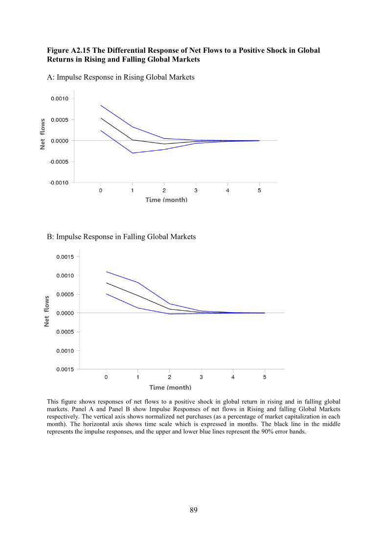
89
Figure A2.15 The Differential Response of Net Flows to a Positive Shock in GlobalReturns in Rising and Falling Global Markets
A: Impulse Response in Rising Global Markets
B: Impulse Response in Falling Global Markets
This figure shows responses of net flows to a positive shock in global return in rising and in falling globalmarkets. Panel A and Panel B show Impulse Responses of net flows in Rising and falling Global Marketsrespectively. The vertical axis shows normalized net purchases (as a percentage of market capitalization in eachmonth). The horizontal axis shows time scale which is expressed in months. The black line in the middlerepresents the impulse responses, and the upper and lower blue lines represent the 90% error bands.
Net
flo
ws
Time (month)
Net
flo
ws
Time (month)

90
Figure A2.16 Impulse Response of Domestic Return to a Shock in Net Inflows
This graph shows a point estimation of impulse response functions with 90% confidence bands derived from aMonte Carlo simulation. The vertical axis shows domestic return in percentage, and the horizontal axis showstime in months. The black line in the middle represents the impulse responses, and the upper and lower bluelines represent the error bands.
Ret
urn
Time (month)

91
Chapter 3: Global Risk Appetite and Foreigners’ Trading

92
3.1 Introduction
Many emerging countries have experienced severe financial crises in their economies
due to sudden reversals of capital inflows. Hence, the question of what determines these
capital flows to emerging countries has received widespread attention in the economics and
finance literature. One important strand of literature focuses on equity flows and tries to
determine key drivers motivating these equity flows to emerging markets. The literature tries
to answer this question by investigating the joint dynamic relationship between equity flows
and local returns. The studies in this literature, mainly investigate this relationship in two
ways. First, they investigate whether equity flows are determined by local past returns, that is,
whether international investors are feedback traders. Second, they focus on the impact of
equity flows on local returns. While analyzing the dynamic relationship from these two
aspects, some studies such as Bekaert et al (2002), Griffin et al (2004), and Richards (2005)
also consider some global factors as global determinants of international capital flows, since
what is documented in many studies with regard to financial crises is that they tend to cluster.
Therefore, the spill-over of sovereign financial crises is not generally accepted to be fully
explained by domestic fundamentals alone.
On this basis, in terms of global factors, Bekaert, Harvey, and Lumsdaine (2002)
consider the world interest rate as an exogeneous variable and Griffin et al (2004) and
Richards (2005) employ broad market stock returns as potential determinants of capital
equity flows. However, in terms of global factors, it is rather interesting to note that no study
in this line of research has studied the effects of global risk appetite on equity flows to
emerging markets. One possible explanation about the reason for the lack of the empirical
studies may be sourced from the belief that funds could not be shifted so quickly
internationally on a daily basis to reflect variations in the risk appetite level.

93
Here, what is particularly interesting to note is that another strand of literature that
investigates the factors that affect emerging market bond spreads (mostly on a daily basis)
gives considerable attention to this factor. However, it is worth pointing out that portfolios of
international investors not only consist of emerging market bonds, but also emerging market
stocks as well and as the risk tolerance of an investor decreases he/she wants to shift his/her
portfolio to a more conservative allocation. International investors might start with
establishing a goal of some certain percent of foreign stocks in his/her portfolio. However,
whatever the mix, if his/her appetite for risk increases or decreases, the percentage of his/her
portfolio devoted to foreign stocks can also be changed in order to adapt to his/her new
investment plan. In this context, if the risk appetite of international investors is constantly
changing then their portfolios should also be balanced constantly in order to meet their risk
tolerance. The balance we are referring to here is the ratio of foreign stocks held by
international investors in their total portfolios. Given the above, from an investor perspective,
this factor deserves particular consideration especially given the recent ongoing credit crisis
or subprime panic started in the USA which causes reversal of capital flows from almost
every emerging stock market. Therefore, this study is the first to provide evidence about the
impact of global risk appetite on the behaviour of foreign investors in emerging markets.
As a second point, our study also diverges from all previous studies by providing a
comprehensive exploration of the return-flow dynamics. The interaction between foreigners’
trading and emerging stock market returns has not been analyzed so far while taking the
changing global and local conditions into consideration. In other words we are not aware of
any study that has examined whether foreigners’ trading strategies with respect to local return
vary with changing global and local conditions. For example, in terms of global conditions,

94
no study has investigated whether foreigners’ trading strategies with respect to emerging
market returns has been different at different global risk appetite levels. On this basis, our
study looks at whether the trading strategy (with respect to local return) followed by
foreigners at times when the global risk appetite is high is similar to the trading strategy
followed by foreigners at times when the global risk appetite is low. No previous study has
tried to answer this question so far in this line of research. However, the answer to this
question is of great importance to policy makers, because, all previous studies uniformly
documented that foreigners engage in positive feedback trading strategies with respect to
local returns, and positive feedback trading is also known to have the potential to push prices
away from fundamentals. Therefore, if foreigners are found to pursue different trading
strategies at different global risk appetite levels regulators can benefit from this information
and introduce different measures at different times to stabilize the market.
As a third point, apart from global conditions, this study also investigates the
interaction between foreigners’ trading and emerging stock market returns in terms of local
conditions. In previous studies, such as Brennan and Cao (1997) and Griffin et al (2004),
foreign investors are suggested to chase recent local market returns due to being
informationally disadvantaged compared to local investors. In this respect, our study seeks to
document whether foreigners chase recent local returns irrespective of the economic
conditions in the emerging country. On this basis, we analyze whether the trading strategy
with respect to local return followed by foreigners at times when the local economy is in a
high growth period is similar to the trading strategy followed by foreigners at times when the
economy is in a low growth period. It is useful to see whether foreign investors engage in
different trading strategies with respect to local return at different points in the business
cycle, since the answer to this question is of great importance to academicians. If we find no

95
difference in their trading strategies across different economic states, our finding can be
regarded as strong evidence that supports a model of Brennan and Cao (1997) which suggests
that foreign investors use recent returns as information signals, as they have an informational
disadvantage in emerging markets. In other words, foreign investors may use only recent
returns as information signals about the expected return of the local market and that is why
they are positive feedback traders irrespective of the local conditions. However, if we find
differences in trading behaviours across states of the economy, foreign investors can be
thought to use other information sources as information signals at different states of the
market rather than chasing the past prices to form expectations about the expected return. It is
here important to note that this thesis, in chapter two, documents different behavioural pattern
for foreign investors in up and down markets in the ISE which shows that foreigners chasing
past returns may not be a general phenomenon. On this basis, the answer to this question
should also be an issue of great concern to regulators in order to be successful at stabilizing
market when introducing measures.
We try to answer the above questions by employing daily trading data from five
emerging stock markets. The markets we analyze are as follows: the Jakarta Stock Exchange,
the Korea Stock Exchange, the Stock Exchange of Thailand, the Taiwan Stock Exchange, and
the Kosdaq Stock Market.
The rest of the chapter is organized as follows: in section 3.2 we provide a review of
the literature addressing the issues mentioned above, together with their theoretical
backgrounds, and we state our hypotheses regarding our research questions. Section 3.3
describes the data. Section 3.4 and 3.5 presents descriptive statistics and also key changes in
the five South-east Asian stock markets respectively. Section 3.6 outlines the methodology

96
employed in this study. Section 3.7 presents results, and section 3.8 summarizes main
conclusion.
3.2 Literature review
In the early 1990s, many developing countries began to liberalize their stock markets.
The restrictions on foreign ownership were relaxed, which usually went hand in hand with
sound macroeconomic and trade reforms. Following these liberalization processes many
emerging countries suffered from financial crises due to sudden capital outflows from their
markets. Therefore, foreigners’ trades are mainly viewed to have a strong influence on equity
prices, and their trading has been closely watched by local market participants. One line of
research studies the joint dynamic relationship between foreign equity flows and local
returns. Early studies in this literature mainly explore whether the trading of foreign investors
is affected by past local returns, because, many academics argue that the trades of foreign
investors are usually influenced by past returns, that is, they buy when prices have risen and
sell when they have fallen. Such behaviour is known as positive feedback trading, and it has
also been shown by theoretical models that investors who pursue positive feedback strategies
can have a destabilizing impact on stock markets. It is therefore of crucial importance to
understand how they trade and their impact on equity prices.
In a similar vein, Clark and Berco (1997), one of the earliest studies in this literature,
test whether current equity flows are caused by past returns in emerging markets, in other
words, whether foreigners pursue any trading strategy in the Mexican stock market. The
study uses monthly data from January 1989 to March 1996 and finds no evidence that
foreigners chase recent prices. Similarly, Choe, Kho, and Stulz (1999) investigate the trades

97
of foreign investors in the Korea stock market for the pre-crisis and during the crisis periods
to see whether they destabilize the stock market. They use daily data beginning on December
2, 1996 and ending on December 27, 1997. In the pre-crisis period, the study finds that
foreign investors tend to follow herding and momentum trading strategy. However, during
the crisis period, the study finds no evidence of herding and positive feedback trading by
foreign investors. Surprisingly, foreign investors are found to sell more in a booming market
relative to bear market periods. This does not accord with the general view that foreigners
flee from emerging equity markets which are crashing. Similar to the study of Choe, Kho,
and Stulz (1999), Kim and Wei (2002) explore the behaviour of foreign investors in terms of
feedback and herding trading in the Korean stock market. The study, analyzing three different
groups of foreign investors, finds no statistical evidence of momentum or contrarian
strategies for any group of foreign investors. However, Kim and Wei (2002) find evidence of
herding behaviour for each type of foreign investor. Furthermore, they find that foreign
individuals tend to herd more than foreign institutions.
Similarly, Grinblatt and Keloharju (2000), analyzing stock investments in the Finnish
stock market from December 1994 through December 1996, document significant evidence
of momentum trading by foreigners. Another recent study is provided by Dahlquist and
Robertson (2004) who study the investment behaviour of foreign investors in the Swedish
market subsequent to the liberalization period. The study, analyzing the period 1993–1998 on
a monthly basis, documents that foreigners tend to pursue a momentum trading investment
style in the Swedish market.
The same issues were also analyzed using larger data sets. For example, Brennan and
Cao (1997), employing quarterly data between the first quarter of 1989 and last quarter of

98
1994, investigate net purchases of US investors in 16 emerging markets and find strong
evidence of positive correlation between current net purchases of US investors and lagged
local equity returns. This suggests that US investors pursue momentum trading strategies in
these emerging markets. Another study by Froot, O'Connell, and Seasholes (2001), which
uses the largest data set in this literature, investigates international equity flows into and out
of 28 emerging countries. The study uses daily data that begins on August 1, 1994 and goes
through December 31, 1998 provided by State Street Bank & Trust, a custodian bank. It finds
very strong evidence that foreign investors follow momentum trading strategies.
In addition, Borensztein and Gelos (2003) contribute to this literature by using a novel
database provided from eMergingPortfolio.com that covers, on a monthly basis, about 80
percent of equity funds worldwide with a focus on emerging markets for the period January
1996 to December 2000. It is the first study on a global scale that aims to document the
behaviour of mutual funds. The study is interested in whether there is evidence of herding
among these emerging market mutual funds during turbulent and during tranquil times and
whether these funds systematically pursue positive feedback or momentum strategies.
Borensztein and Gelos (2003) find some evidence of herding behaviour among mutual funds,
which is statistically significant, but smaller than expected. They also find some evidence that
emerging market mutual funds tend to pursue positive feedback trading. In sum, herding and
momentum trading seems to be an observed fact among emerging market funds.
While analyzing the dynamic relationship from these two points of view, some studies
also consider some global and local factors as determinants of international capital flows. The
earliest study in that respect is undertaken by Chuhan, Claessens, and Mamingi (1998) who
examine the factors that motivate US equity and bond flows to nine Latin American and nine

99
Asian countries. The study uses monthly data beginning in January 1988 and ending in
September 1992. They attempt to understand to what extent the capital inflows are
determined by global factors and to what extent by country-specific factors. The two key
global variables employed in the study are US interest rates and US industrial production.
The study also includes the country's credit rating, the secondary market price of a country's
debt, the price-earnings ratio, and the domestic stock market return as explanatory variables
for country specific factors. The study finds that both global and country-specific factors have
significant value in explaining these capital inflows. The empirical results suggest that the
slowdown in the US economy and drop in US interest rates have almost a similar significant
effect as country-specific factors in explaining the flows to the Latin American countries.
However, for the Asian countries it appears that country-specific factors have nearly three to
four times more significant effects compared to global factors in explaining these flows.
Chuhan et al (1998) also find evidence that bond and equity flows have different sensitivities
towards explanatory variables. Equity flows appear to be more sensitive relative to bond
flows to US industrial activity and US interest rates. As expected, equity flows are also found
to be more sensitive than are bond flows to a country's price-earnings ratio and the return on
domestic stock markets.
Given the results above, a point worth mentioning here is that the study by Chuhan et
al (1998) employs a panel regression approach rather than the VAR approach, which is not
common in this literature due to the endogenous relationship between foreign equity flow and
local market returns. A critical point here to note is that following this study no subsequent
work, which investigates the effects of global factors on equity flows, has employed the same
approach in this literature which implicitly calls their findings into question For example,
later on, Bekaert, Harvey, and Lumsdaine (2002) examine the behaviour of US equity flows
100
to 20 emerging markets using a vector-autoregressive (VAR) framework as a main tool, as in
Froot et al (2001), but include two additional variables besides their bivariate VAR model for
portfolio flows and local asset returns. As a first variable Bekaert et al (2002) add a world
interest rate that has been thought to have a significant effect on capital flows. As a second
variable, they add local dividend yields as a measure for the cost of capital, since it is
believed to capture permanent price effects better than average returns. Bekaert et al (2002)
find that a shock to world interest rate has no contemporaneous effect on net equity flows.
However, after one period, small increases generally appear in net equity flows subsequent to
a negative shock. In addition, the hypothesis that capital flows are driven by changes in
expected returns or past returns, in other words whether foreign investors are “return chasers”
or “momentum traders” is examined and they find evidence of momentum trading rather than
return chasing.
Another study by Karolyi (2002) investigates whether foreign trading activity in
Japan worsened the impact of the Asian crisis on Japanese markets, or whether it just
reflected typical momentum trading behaviour. The data come from weekly reports that
include the yen value of aggregate purchases and sales of Japanese stocks by foreigners. In
terms of local factors, besides local returns, the study considers currency returns and employs
a tri-variate vector auto-regression (VAR) model to test the joint dynamics of foreign
portfolio flows and equity market and currency returns. The study finds consistent evidence
of momentum trading among foreign investors during and after the Asian financial crisis.
Fluctuations in the yen/dollar returns and Nikkei index are both found to have a significant
impact on foreign net purchases. Karolyi (2002) finds no evidence that foreign net purchases
have a significant impact on stock prices. The study concludes that foreign trading activity
did not destabilize the markets during the Asian financial crisis.

101
Even though the study by Froot et al (2001) was the most comprehensive one that has
been done so far, since their data set captures only custodian clients from State Street and
only uses bivariate VAR between equity flows and local returns, Griffin, Nardari, and Stulz
(2004) attempt to document whether their results can be valid for foreign investors in general
when including mature market returns. Their sample consists of precise daily data of all
foreign investors in nine emerging markets that begin from January 1996 for Korea,
Indonesia, and South Africa, 1997 for Taiwan and Thailand, 1998 for India, Sri Lanka, and
Slovenia, and 1999 for the Philippines. The daily analysis for all countries ends on February
23, 2001 except for Slovenia which ends on January 31, 2001. Griffin et al (2004) find that in
addition to local market returns, lagged returns in mature markets such as the USA are
helpful in explaining equity flows into emerging countries. Even though local market returns
are found to have an economically significant effect on flows, equity flows are found to be
more responsive to past US returns compared to local returns. The results are also robust after
controlling for exchange rate effects. On the other hand, the study finds very limited evidence
that foreign investors follow past local and international returns when testing the prediction
of their model at the weekly frequency.
Another study by Richards (2005), which is very close in design to the paper by
Griffin et al (2004), documents the similar evidence. It uses daily data over 1999-2002 of all
foreign investors’ net purchases in six Asian equity markets. The five markets (namely the
Jakarta Stock Exchange, the Korea Stock Exchange, the Philippine Stock Exchange, the
Stock Exchange of Thailand, and the Taiwan Stock Exchange) that were also studied by
Griffin et al (2004)) are studied in this paper in addition to the Kosdaq Stock Market. The
foreign returns are found to have more significant explanatory power than local returns on

102
equity flows and the study considers possible explanations for these findings similar to those
of Griffin et al (2004). Richards (2005) suggests that it is not likely to be due to
microstructure effects or portfolio rebalancing effects of which the latter are implicitly
modeled in Griffin et al (2004) study. Instead, he suggests that broad market shocks are of
central importance to foreign investors while revising their expectations for emerging
markets. He supports his suggestion with a consistent finding about the returns relationship
between US technology stocks and the technology-oriented Korean and Taiwanese markets.
He finds that the returns on US technology stocks have more explanatory power on inflows
into these two markets, which can be viewed as news about fundamentals. He suggests that it
may also be due to behavioural reasons rather than extracting rational information.
Finally, after having summarized all the relevant studies in the literature, in terms of
global factors, it is interesting to note that no study in this line of research has studied the
effects of global risk appetite on equity flows to emerging markets. However, one strand of
literature that investigates the factors that affect emerging market bond spreads, gives
considerable attention to this factor. For example, McGuire and Schrijvers (2003), employing
25 emerging country bond data, examine whether there are common forces that affect
movements in emerging market bond spreads. The study applies principal factor analysis to
investigate the common sources of variation in bond spreads and finds one single significant
factor that drives most of the variation in bond spread changes. The study also documents a
high correlation between this common factor and changes in investors’ appetite for risk and
concludes that changes in investors’ attitudes towards risk play an important role in
explaining the common variation in emerging market bond spreads.

103
Rozada and Yeyati (2008) examine the variability in emerging market bond spreads to
see whether exogenous factors explain a substantial part of this variability. The study,
employing bond data from 33 emerging markets, finds that global factors such as investors’
appetite for risk (proxied by high yield corporate bonds), global liquidity (proxied by the
yield of US Treasury notes, 10 year constant maturity) and contagion (such as the Russian
default) explain a large portion of the variability in these emerging market bond spreads.
Ciarlone, Piselli, and Trebeschi (2008) analyze to what extent changes in emerging
market bond spreads can be attributed to specific factors, rather than to global factors. The
study employs factor analysis and finds a single common factor that can explain a large part
of the correlation between emerging market bond spreads. This single common factor is also
found to be sensitive towards the movements in the degree of investors risk aversion and
volatility in financial markets.
Finally, Herrero and Ortiz (2005) investigate whether global risk aversion has
significant explanatory power in explaining Latin American bond spreads, after accounting
for the effect of its main determinants such as US economic growth and the US long term
interest rates. The study finds significant evidence that global risk aversion is positively
related to Latin American bond spreads and its impacts on bond spreads is found to vary
across countries and through time.
3.2.1 Shortcomings of previous studies and motivation
Given the above literature review, this study presents shortcomings of previous
studies and its motivations with their stated hypotheses.

104
It is clear from the above review that no study has investigated the effects of global
risk appetite on equity flows to emerging markets, whereas it is of central importance in the
literature that investigates the factors that affect emerging market bond spreads. This is a very
interesting point as portfolios of international investors not only consist of emerging market
bonds but also emerging market stocks. Therefore, this factor should also attract the attention
of professionals and practitioners especially given the recent ongoing global credit crisis
started in the USA which led to a sudden stop or reversal of capital inflows in almost every
emerging stock market. In view of this, we test whether global risk appetite has a significant
effect on equity flows to emerging markets. Thus, our first hypothesis can be stated as below:
Hypothesis (1): global risk appetite has a significant effect on the trading behaviour of
foreign investors in emerging markets.
Previous studies have not investigated the dynamic relationship between the
foreigners’ trades and local returns while taking into account global risk appetite. If
foreigners’ trades are thought to be affected by the global risk conditions then it is possible
that they follow different trading strategies at different global risk appetite levels. Then, a
natural question to ask of our foreigners’ trading data is whether there is any evidence of
foreigners following different trading strategy in any of the high and low risk appetite periods
when compared with the whole period.
On this basis, our second hypothesis can be stated as:
Hypothesis (2): the trading strategies that foreigners follow in high and low global risk
appetite levels are different from each other.

105
In a similar vein, it is clear from the literature review that previous studies have not
provided any evidence about how foreigners behave with respect to local returns at different
points in the local business cycle. It is possible that their trading strategies can differ across
high and low growth periods if they use other sources as information signals rather than
chasing past prices, because investors are found to consider the same type of news to be bad
in some stages of the business cycle and good in others (see eg., McQueen and Roley, 1993;
Li and Hu, 1998). If they differed it would be highly relevant for regulators while introducing
measures to enhance the stability of the stock market. In order to examine this issue our third
hypothesis can be stated as:
Hypothesis (3): The trading strategies that foreigners follow in high and low states of the
local economy are different from each other.
In a nutshell, our study makes the following contributions:
- We provide the first evidence about the effect of global risk appetite on the net
purchases of foreign investors in emerging stock markets.
- We provide the first evidence about whether foreigners engage in different trading
strategies with respect to local returns at high and low global risk appetite levels.
- We provide the first evidence about whether foreigners follow different trading
strategies with respect to local returns at different states of the economy.
3.3 Data
We investigate the trading behaviour of foreign investors in five emerging markets.
The markets are the Jakarta Stock Exchange (JSE), the Korea Stock Exchange (KOSPI), the

106
Stock Exchange of Thailand (SET), the Taiwan Stock Exchange (TSE), and the Kosdaq
Stock Market. All markets except for the Kosdaq are main boards. Kosdaq is the second
board in South Korea, but its market capitalization is much higher than many main boards in
emerging markets. Richard (2005) also analyzes the same five boards. In order to investigate
trading behaviour of foreign investors in more detail there is clearly a need for actual trading
data. Our study uses daily purchases and sales values for foreign investors in these five stock
markets. Daily purchases and sales values for foreign investors are obtained from the related
exchanges and from CEIC (data company), a secondary provider. The available data begin in
January 1995 for Thailand and Indonesia, 1999 for Kosdaq, 2000 for Taiwan and 2001 for
the KOSPI index. The end date for daily analysis is May 15, 2008 for all markets. However,
we prefer the observation period to be the same across all markets in order to make the
analysis homogeneous. Therefore, our observation period starts in June 2001 for all markets.
Daily net purchases of investors ( tf ) are expressed in terms of percent of the previous day’s
market capitalization.
)( tt sellbuy 100tf × (1)
( 1) ttalizationmarketcapi
Daily market capitalization data for each market are obtained from Datastream. We
use the term “net purchases” as a measure of purchases minus sales. Net purchases are
normalized by dividing by the related previous day’s market capitalizations as in Griffin et al
(2004) and Richards (2005). Such normalization is useful to understand how important is the
net demand compared to total supply of available shares (Griffin et al., 2004). We use this
measure as a direct indicator of net investor demand for all stocks in these five stock markets.
The results of Augmented Dickey-Fuller unit root tests of the normalized five variables
corresponding to each market are shown in Table 3.1.

107
Correlations between net inflows into different markets are also reported in Table 3.2.
Since there are five market returns we have ten pair of correlations and nine out of these ten
correlations are found to be positive. The coefficients of pair-correlations among four
markets, namely; the KSE, KOSDAQ, TWSE and THAILAND are found to be more than
0.20. From these correlations there is some prima facie evidence that there are some common
factors that primarily drive these net flows. This will be tested formally in the next section.
Table 3.2: Correlations Between inflows into Different Markets
KSE KOSDAQ TSE JXS SETKorea (KSE) 0.34 0.4 0.02 0.25Korea (Kosdaq) 0.34 0.2 -0.03 0.13Taiwan (TSE) 0.4 0.2 0.03 0.32Indonesia (JSX) 0.02 -0.03 0.03 0.07Thailand (SET) 0.25 0.13 0.32 0.07
This table reports the correlations between daily net inflows into different markets. Net inflows are normalizedby the previous-day market capitalization.
Daily return data for local market indices are collected from Datastream. Since recent
comprehensive studies such as Griffin et al (2004) and Richard (2005) find that net foreign
equity flows to emerging markets give more significant response to past US returns relative
to local market returns in most emerging markets they investigated, we employ the S&P 500
return index as a proxy for the global factor obtained from http://finance.yahoo.com/ which is
adjusted for stock splits and dividends. The S&P 500 market returns are measured as the
daily log-differenced change in the price index.
We also use daily exchange rate changes as a possible determinant of net foreign
equity flows to emerging market as in Griffin et al (2004), since a depreciation of the local
currency can lead to more foreign inflows. Data for exchange rates for countries are obtained

108
from Datastream except for Indonesia, which is obtained from the central bank of Indonesia.
Since in this study we also explore the effects of global risk appetite on the behaviour of
foreign investors in emerging markets, as a proxy for risk appetite, we use the VIX (the
Chicago Board Options Exchange Volatility Index) obtained from the CBOE which is
commonly treated as a quick and easy proxy for risk appetite in many studies such as
Ciarlone, Piselli, and Trebeschi (2008) and Rozada and Yeyati (2008). It is often referred to
as the fear index. Investors buy and sell S&P 500 index options to change the amount of risk
to which they are exposed. It measures the cost of using options as insurance against declines
in the S&P 500. A change in global risk appetite is measured as the daily log-differenced
change in the VIX index.

109
Table 3.1: Unit root test for normalized net flows
Null Hypothesis: Normalized net flows has a unit rootExogeneous: constant--------------------------------------------------------------------------------------------------------------------------------------------------------------------------------------------------------------------------
Thailand Korea Kosdaq Indonesia Taiwanstat Prob* stat Prob* stat Prob* stat Prob* Stat Prob*
Augmented Dickey-Fuller test statistic: -17,878 0.00 -13.485 0.00 -19.998 0.00 -38.719 0.00 -15.104 0.00--------------------------------------------------------------------------------------------------------------------------------------------------------------------------------------------------------------------------Test critical values: 1% level -3.478
5% level -2.88210% level -2.578
This table shows unit root test for net flows in each market normalized by the contemporaneous market capitalization. ADF (Augmented Dickey-Fuller) test is employed as a unitroot test. ADF test is estimated that includes only constant in the test regression with automatic lag length selection based on Schwarz Information Criterion with a maximum laglength of 24. * denotes associated one-sided p- value for the ADF test statistic. Lag lengths of 0, 2, and 3 are selected for Indonesia, Taiwan and Kospi respectively and lag lengths of1 are selected for Thailand and Kosdaq automatically based on the Schwarz Information Criterion.

110
3.4 Key changes in the five South-east Asian stock markets
A chronology of regulations on foreign investment is also given below for each
country to see the key changes in these markets in terms of foreign investment opportunities.
3.4.1 Thailand
According to IFC (International Finance Corporation), Thailand officially liberalized
its stock market in December 1988. Before that time, it was not possible for international
investors to invest directly in Thai stocks. In 1995, the ratio of foreign ownership in Thai
companies was restricted to a maximum of 49%, except for financial institutions. The limit
was 25% for financial companies, which was then gradually lifted to 49%, beginning in June
1997 on a case-by-case basis. The SET eased the trading of shares among foreign investors
that exceeded their foreign ownership limit by carrying out these trades on a special foreign
board. However, in 2001, the SET issued a new trading instrument called NVDR (Non-
Voting Depository Receipt) which allows foreigners to buy more than 49% of the shares
while receiving all financial benefits except for voting rights.
3.4.2 Korea (Kospi and Kosdaq indices)
Foreign investors were officially allowed to invest in the Korean stock market in
January 1992. Initially, foreigners were permitted to own up to 10% of Korean companies in
aggregate. This limit was raised to 12% in December 1994, to 15% in July 1995 and to 18%
in May 1996. Then foreign ownership was again relaxed to 20% in September 1996 and to
23% in May 1997. Restrictions on foreign ownership were lifted on Korean stocks in May
1998, except for some specific industries, such as the Korea Electric Power Corp (KEPCO),

111
the steel industry (POSCO), mining, air transportation and information and communication
which were restricted to a limit of 30%, 30%, 49.99%, 49.99%, and 33% respectively. Unlike
other industries, radio broadcasting and television broadcasting later on were completely
closed to foreign investment in 2002.
3.4.3 Indonesia
Indonesia officially opened its stock market to foreigners in September 1989. As the
stock market was liberalized, foreign investors were allowed to purchase up to 49% of all
domestic companies excluding financial companies. The ownership limits in financial
companies were then raised to 49% as well in January 1992. In September 1997, the
authorities allowed foreigners to purchase unlimited shares of domestic firms excluding
banking shares. They then removed the barriers to foreigners in retail trade and wholesale
trade banks in March 1998 and April 1998 respectively. Like Korea, some sectors were
closed to foreigners in 2002. Some of these sectors are germ plasm cultivation, lumber
contractors, forest concessions, TV, radio, print media, film and cinema. Some of the
industries of which foreigners are allowed to own up to 45% are airport/seaport construction
and operation, transmission and distribution, electricity production, shipping, railway service,
drinking water, atomic power plants, and certain medical services.
3.4.4 Taiwan
Official stock market liberalization took place in January 1991. Qualified Foreign
Institutional Investors (QFII) were allowed to invest in Taiwan domestic shares up to no more
than 12% of the total market capitalization and no more than 6% of individual ownership.
The limit on foreign ownership then was raised to 20% in March 1996 and to 25% of the total

112
market capitalization in December 1996. Finally, QFII were permitted to buy up to 50% of
domestic listed companies in March 1999. Although heavy foreign investment was still
restricted in certain industries such as finance in 2003, these barriers are gradually coming
down.
3.5 Methodology
Within each country, we examine our research questions by using Vector
Autoregression (VAR) methodology, which enables us to study the dynamic relationship
between flows and returns. Apart from these two endogenous variables we try to document
the effects of global risk appetite on the equity flows and, since previous studies such as
Griffin et al (2004) and Richards (2005) strongly suggest the inclusion of broad market
returns as determinants of net inflows for a typical emerging country, we augment our
bivariate-VAR model with the global risk appetite and broad market return, both of which are
affected only by their own lags. This enables a more accurate characterization of the joint
dynamic relationship between flows and domestic returns. The advantage of utilizing this
specification instead of a standard VAR is that none of the lags of equity flows and local
returns affect the global risk appetite and broad market returns, but contemporaneous values
of them are affected by the instantaneous and lagged values of global risk appetite and broad
market returns. Thus, global risk appetite and broad market returns are treated as exogenous
variables. The system is estimated separately for each market as seemingly unrelated
regressions (SURs), since the right-hand side variables explaining global risk appetite and
global return are different. In line with the common treatment in the literature, net flows are
assumed to have a contemporaneous effect on local returns, but not vice versa. Local returns

113
can only have an effect on equity flows with a lag. In other words, current returns can only
affect future flows and returns.
Thus we follow Griffin et al (2004), which can be specified as:
(2))()()()()(
,
,1
1,
1,
2221
1211
,
,
,
,
rti
fti
titi
ti
ri
fi
ti
ti LArf
LbLbLbLb
rf
x
Where fi,t denotes the daily net foreign flows (buy value - sell value) normalized by previous-
day market capitalization, for country i. ri,t denotes the daily market returns for country i. The
α’s represent constant intercept terms, b(L) denotes a polynomial in the lag operator L, and
fti , and r
ti , are zero-mean error terms that are assumed to be intertemporally uncorrelated.
xt is a vector that includes daily broad market returns and global risk appetite as push
(sourced from outside of the country in question) factors and the local exchange rate as a pull
(sourced from inside of the country in question) factor which are all considered to be
exogenously determined.
A point worth mentioning here is that since all Asian-Pacific countries are in different
time zones relative to the USA, the Pacific exchanges are closed when the US market opens
for the day. Therefore, we employ the previous overnight S&P 500 returns and global risk
appetite levels in our VAR rather than the same day value. Furthermore, since every market
has specific holidays it is inevitable that we have missing observations. Following Richards
(2005) we deal with this problem in such a way that if there is no trading for the emerging
market in question, that day is omitted and the price change is calculated from the last time
that the market was open. This way, continuous series of foreign inflows and local returns are
obtained for the emerging market. In a similar vein, we also eliminate any day when the US

114
market is closed and we aggregate net purchases of foreigners where the local market was
open while the US market closed.
Having specified the model and given details about how to deal with the missing
observations in the VAR framework, we now move to determine the number of lags to
include in the VAR equations for the five markets. On this basis, table 3.4 below shows the
optimal lag length for the five markets as suggested by both the Schwarz criterion (SIC) and
the Hannan–Quinn information criterion (HQC).
As can easily be seen from table 3.5 the Hannan–Quinn information criterion (HQC)
suggests the optimal lag lengths of one for Indonesia, two for KOSDAQ, three for Taiwan
and Thailand and four for KOSPI. Since we have large sample sizes the degrees of freedom is
not a concern. Therefore, we choose a common lag length of four lags for all five markets, as
done in Richards (2005) and Griffin et al (2004), which also homogenises the analysis across
markets. Following griffin et al (2004), the lag length of the exogeneous variables are also
restricted to be the same as the endogenous variables across markets.

115
Table 3.3: VAR lag order selection criteria (01/06/2001-16/05/2008)
KOSPI KOSDAQ
Lag SC HQ Lag SC HQ
0 -18.29139 -18.29552 0 -18.26413 -18.268251 -18.55905 -18.57143 1 -18.47014 -18.482492 -18.585* -18.60613 2 -18.47331* -18.4939*3 -18.58532 -18.61421 3 -18.46187 -18.490694 -18.57747 -18.6146* 4 -18.4493 -18.486365 -18.56436 -18.60976 5 -18.43739 -18.482686 -18.55362 -18.60728 6 -18.42055 -18.474077 -18.54216 -18.60407 7 -18.40555 -18.467318 -18.52552 -18.59568 8 -18.39336 -18.463369 -18.51016 -18.58857 9 -18.37893 -18.45716
10 -18.49807 -18.58474 10 -18.36266 -18.4491311 -18.48522 -18.58014 11 -18.34902 -18.4437212 -18.47062 -18.57379 12 -18.33223 -18.43517
INDONESIA TAIWAN
Lag SC HQ Lag SC HQ
0 -8.88272* -8.886869 0 -18.46652 -18.470641 -8.876804 -8.88922* 1 -18.79862 -18.810972 -8.863166 -8.883871 2 -18.82748* -18.848083 -8.849126 -8.878113 3 -18.82746 -18.8563*4 -8.835697 -8.872966 4 -18.81648 -18.853555 -8.825551 -8.871102 5 -18.80029 -18.84566 -8.808866 -8.862699 6 -18.78383 -18.837387 -8.793304 -8.855418 7 -18.77197 -18.833768 -8.775825 -8.846221 8 -18.75477 -18.82489 -8.758774 -8.837452 9 -18.74209 -18.82036
10 -8.742071 -8.829031 10 -18.7275 -18.81411 -8.729114 -8.824356 11 -18.71196 -18.806712 -8.712735 -8.816259 12 -18.69595 -18.79893
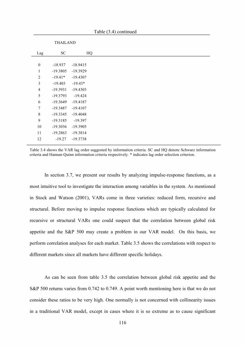
116
Table (3.4) continued
THAILAND
Lag SC HQ
0 -18.937 -18.94151 -19.3805 -19.39292 -19.41* -19.43073 -19.403 -19.43*4 -19.3931 -19.43035 -19.3793 -19.4246 -19.3649 -19.41877 -19.3487 -19.41078 -19.3345 -19.40489 -19.3185 -19.397
10 -19.3036 -19.390511 -19.2863 -19.381412 -19.27 -19.3738
Table 3.4 shows the VAR lag order suggested by information criteria. SC and HQ denote Schwarz informationcriteria and Hannan-Quinn information criteria respectively. * indicates lag order selection criterion.
In section 3.7, we present our results by analyzing impulse-response functions, as a
most intuitive tool to investigate the interaction among variables in the system. As mentioned
in Stock and Watson (2001), VARs come in three varieties: reduced form, recursive and
structural. Before moving to impulse response functions which are typically calculated for
recursive or structural VARs one could suspect that the correlation between global risk
appetite and the S&P 500 may create a problem in our VAR model. On this basis, we
perform correlation analyses for each market. Table 3.5 shows the correlations with respect to
different markets since all markets have different specific holidays.
As can be seen from table 3.5 the correlation between global risk appetite and the
S&P 500 returns varies from 0.742 to 0.749. A point worth mentioning here is that we do not
consider these ratios to be very high. One normally is not concerned with collinearity issues
in a traditional VAR model, except in cases where it is so extreme as to cause significant

117
estimation problems. With a VAR, we are generally interested in the overall behaviour of the
model rather than in the individual coefficient values, or the significance of individual
coefficients. A reasonable amount of correlation is to be expected in any VAR model, almost
by definition.
Table 3.4: The correlations between VIX and S&P 500 returns
Thailand -0.749Kosdaq -0.748Indonesia -0.748Taiwan -0.745Kospi -0.742
This table shows the correlations between VIX and S&P 500 returns in each sample. The S&P 500 marketreturns are measured as the daily log-differenced change in price index. VIX changes is also measured as thedaily log-differenced change in volatility index.
3.5.1 Reaction to lagged local returns conditional on the state of the economy
As a second point we explore whether foreign investors follow the same trading
strategy with respect to local returns, irrespective of local conditions. In other words, we look
at whether they engage in the same trading strategy across high and low state of the economy.
We look at this issue by estimating VAR regressions of flows on local return with dummy
variables. We construct two separate return series that correspond to the periods of high and
low economic growth as below.
r high, t = HIGH t r t
r low, t = LOW t r t
Where,
HIGHt = 1 if the local economic growth is in the high state at time t, and zero otherwise;

118
LOWt = 1 if the local economic growth is in the low state at time t, and zero otherwise;
We examine this issue by following the similar methodology in specification (2) but
replacing the new constructed local return series in place of the local return series. In other
words, we have two VAR system estimations. One includes high state returns in place of
local returns the other one includes low state returns in place of local returns. A point worth
clarifying here is that since we analyze the issue by looking at the cumulative impulse
responses in two different VAR systems, we do not employ wald tests as is typically
employed to determine whether the coefficients are significantly different in a classical linear
regression or in a system of regressions. Instead, we examine the cumulative impulse
responses of foreigners’ net purchases to an innovation in local returns individually in terms
of sign and significance criteria in the two different states of the economy.
3.5.1.1 Classification of economic states
In order to explore whether foreigners’ response to local return changes across
different stages of the local business cycle, we need to classify the different levels of
economic activity. To do so, we follow McQueen and Roley (1993) and use a seasonally
adjusted monthly industrial production index for each emerging country in identifying the
states of the local economy as a boom, recession and normal period.18 To obtain three
different states of the economy, we regress the actual log of industrial production on a
constant and trend. Then we add and subtract a constant from the trend to create the upper
and lower bounds as can be seen in figure 3.1 through figure 3.4. When the log of industrial
18 If the country in question was the USA other methods such as the NBER business cycle turning points or theexperimental coincident index which was constructed by Stock and Watson (1989) would easily be employed indetermining the state of the economy as alternative methods. However, for emerging markets, the McQueen andRoley (1993) methodology is the most applicable one.

119
production (LNIP) is above the upper bound about 25 percent of the time it is denoted as
"high" economic activity. When it is below the lower bound about 25 percent of the time it
indicates low economic activity. The remaining observations between the bounds denote
"Medium" economic activity.
We begin with Thailand, which is shown in figure 3.1. We construct the bounds for
the industrial production symmetrically. The deviations from the industrial production trend
are chosen as +0.0203 and – 0.0203 for the upper and lower bounds respectively, which puts
25 percent of the observations in the high state and 25 percent of the observations in the low
state. However, if the bounds for the industrial production were constructed symmetrically
for other markets the best approximations would be achieved, for Taiwan by the constants
between 0.0236 and 0.0239 which would put about 25 percent in the high state and about
16.7 percent in the low state, for Korea by the constants between 0.01297 and 0.01293 which
would put about 25 percent in the low state and about 26.2 percent in the low state, for
Indonesia by the constants between 0.0259 and 0.0264 which would put about 35.7 percent in
the high state and about 26.2 percent in the low state. Therefore, the bounds are not
constructed symmetrically for these markets. Instead the deviations from the industrial
production trend are chosen as, +0.0236 and – 0.013 for the upper and lower bounds
respectively for Taiwan, +0.013 and – 0.01297 for the upper and lower bounds respectively
for Korea, +0.043 and – 0.0284 for the upper and lower bounds respectively for Indonesia.
These constructed bounds put 25 percent of the observations in the high state and 25 percent
of the observations in the low state for these markets.

120
Figure 3.1: Natural log of industrial production, actual and bounds.
A: Natural log of industrial production, actual and bounds (Thailand).
B: Natural log of industrial production, actual and bounds (Taiwan).
4.5
4.6
4.7
4.8
4.9
5
5.1
5.2
5.3
5.420
01-
5
200
1-8
200
1-11
200
2-2
200
2-5
200
2-8
200
2-11
200
3-2
200
3-5
200
3-8
200
3-11
200
4-2
200
4-5
200
4-8
200
4-11
200
5-2
200
5-5
200
5-8
200
5-11
200
6-2
200
6-5
200
6-8
200
6-11
200
7-2
200
7-5
200
7-8
200
7-11
200
8-2
Ln o
f (I
P)
year
ln(IP)
upper
lower
4.2
4.3
4.4
4.5
4.6
4.7
4.8
200
1-6
200
1-9
200
1-12
200
2-3
200
2-6
200
2-9
200
2-12
200
3-3
200
3-6
200
3-9
200
3-12
200
4-3
200
4-6
200
4-9
200
4-12
200
5-3
200
5-6
200
5-9
200
5-12
200
6-3
200
6-6
200
6-9
200
6-12
200
7-3
200
7-6
200
7-9
200
7-12
200
8-3
Ln o
f (I
P)
year
lnip
upper
lower

121
C: Natural log of industrial production, actual and bounds (Indonesia).
D: Natural log of industrial production, actual and bounds (Korea).
Figure 3.1 shows actual log of industrial production with its constructed upper and lower bounds in panel A, B,C, and D for Thailand, Taiwan, Indonesia, and Korea respectively.The vertical axis shows natural log value ofindustrial production net purchases. The horizontal axis shows time scale beginning in June 2001 and ending inMay 2008. The blue line represents the actual log of industrial production, while red and blue line representupper and lower bounds respectively.
4.5
4.55
4.6
4.65
4.7
4.75
4.8
4.85
4.920
01-
620
01-
920
01-
1220
02-
320
02-
620
02-
920
02-
1220
03-
320
03-
620
03-
920
03-
1220
04-
320
04-
620
04-
920
04-
1220
05-
320
05-
620
05-
920
05-
1220
06-
320
06-
620
06-
920
06-
1220
07-
320
07-
620
07-
920
07-
1220
08-
3
Ln o
f (I
P)
year
ln
upper
lower
4.2
4.3
4.4
4.5
4.6
4.7
4.8
4.9
200
1-6
200
1-9
200
1-12
200
2-3
200
2-6
200
2-9
200
2-12
200
3-3
200
3-6
200
3-9
200
3-12
200
4-3
200
4-6
200
4-9
200
4-12
200
5-3
200
5-6
200
5-9
200
5-12
200
6-3
200
6-6
200
6-9
200
6-12
200
7-3
200
7-6
200
7-9
200
7-12
200
8-3
Ln o
f (I
P)
year
lnip
upper
lower

122
In order to find a proxy for the economic states several methods could be employed
when the country in question was the USA. For instance, we could use the experimental
coincident index (XRIC) which was constructed by Stock and Watson (1989). The XRIC
shows the probability that the economy is in recession. Furthermore, two alternative recession
dummies could also be employed for the USA. First, standard NBER business cycle turning
points could be employed which is commonly used in the literature. Second, we could also
use Chicago Fed National Activity Index (CFNAI) which is a principal component of 85
economic indicators.
However, when coming to emerging markets, we don’t have too many alternatives to
employ. The McQueen and Roley (1993) methodology, which identifies the states of the
local economy as a boom, recession and normal period via using industrial production, seems
to be the most applicable one.
3.5.2 Reaction to lagged local returns conditional on the state of global conditions
Another important issue is whether foreign investors react differently to local returns
across different global conditions. If risk tolerance of a global investor changes he/she may
follow a different trading strategy with respect to local returns to adopt to his/her new
investment plan that meets his/her new risk tolerance. We explore this issue by estimating
VAR regressions of flows on local returns with dummy variables. We construct two separate
return series that correspond to the periods of high and low global risk appetite levels as
below.

123
r high, t = HIGH t r t
r low, t = LOW t r t
Where,
HIGHt = 1 if the global risk appetite is in the high level at time t, and zero otherwise;
LOWt = 1 if the global risk appetite is in the low level at time t, and zero otherwise;
We examine this issue by again following the VAR methodology as in specification
(2), but using the newly constructed return series in place of the whole return series.
3.5.2.1 Classification of states of the global risk appetite
In order to investigate whether foreigners’ response to local return varies across
different global conditions, we need to classify the different levels of global risk appetite. We
use the VIX index to determine the global risk appetite levels. It is better to see the historical
levels of VIX to decide whether there is any upward or downward trend in our observation
period. This is important because, if there is any trend we will follow the McQueen and
Roley (1993) methodology and regress the actual log of the VIX value on a constant and
trend. Then we will add and subtract a constant from the trend to create the upper and lower
bounds as explained in the previous section to determine the economic states for each
country. But if there is no trend there will be no need to create the upper and lower bounds
following this method.
Before moving to the historical time series graph of the VIX it is useful to note that
we prefer the observation period to be the same across five markets in order to make the
analysis homogeneous. Therefore, the VIX period begins in June 2001 and ends in May 15,

124
2008 for all markets. Since every market has specific holidays we calculate related global risk
appetite levels for each market by taking this fact into consideration. However, this issue
makes a very small difference across countries. Therefore, for the sake of generality, we
show only historical time series graph of the VIX index when the US market is open between
June 2001 and May 15, 2008.
When looking at figure 3.2 we do not observe any trend in the historical VIX index
levels within our observation periods. Therefore the trending method, as was employed in the
previous section for determining the economic states, is not used to create the upper and
lower bounds. Instead, we determine the relative standing of each VIX value within our
observation period and denote “high” which has a value above the 75th percentile and denote
“low” which has a value below the 25th percentile.
Figure 3.2 Historical VIX index values (06/2001-05/2008)
Figure 3.2 shows VIX index values with its constructed upper and lower bounds.The vertical axis shows actualVIX values. The horizontal axis shows time scale beginning in June 2001 and ending in May 2008. The blueline represents the actual VIX values, while red and green line represent upper and lower bounds respectively.
5
10
15
20
25
30
35
40
45
50
6/1/01 6/1/02 6/1/03 6/1/04 6/1/05 6/1/06 6/1/07
Vix
val
ue
time
vix
upper bound
lower bound

125
3.6 Descriptive statistics
In this section, we provide detail summary statistics for all the series used in our
empirical analysis which includes five main variables namely net inflows, local returns, local
exchange rate, S&P 500 and VIX. Table 3.5 shows summary statistics of net flows for each
country in addition with the corresponding market capitalizations.
When looking at the Table 3.5 we see that the means of net inflows in each country
are positive showing that foreigners have been net buyer on the average since June 2001.
Standard deviation of net inflows relative to its mean is very high in the KOSPI market
compared to standard deviations in other markets. In other words, net inflows in the Kospi
markets experienced very high volatility during our observation period. In terms of skewness,
net inflows in Indonesia are strongly positively skewed, whereas net inflows in other markets
are slightly positively or negatively skewed.
Table 3.5 Summary statistics of net flows / Market Capitalization by country
THAILAND(SET) INDONESIA(JSE) TAIWAN(TSE) KOREA(KOSPI) KOREA(KOSDAQ)
mean 3.18E-05 0.000134 0.000104 1.44E-06 5.00E-05maximum 0.002991 0.007609 0.003575 0.002362 0.002835minimum -0.004663 -0.002607 -0.002929 -0.001945 -0.002932std.dev 0.000383 0.000489 0.000451 0.00041 0.000389skewness -0.359179 6.050968 -0.145205 0.756409 0.081829kurtosis 24.47175 68.71866 8.051955 6.879968 13.64756
Jarque-bera 31866.32 307740.5 1776.457 1200.264 7871.659probability 0 0 0 0 0
observation 1657 1654 1665 1661 1661
Market Capitalization 197129 211692 663716 1016005 106601

126
This table shows summary statistics of net inflows (divided by the market capitalization) and marketcapitalization in million USD dollar for each country. Observation period are the same for each market whichstarts in 01/06/2001 and goes through 16/05/2008.
For the kurtosis values, all net inflow series exhibit high levels of kurtosis showing
that all series are leptokurtic. Especially net flows in Indonesia are very leptokurtic with the
kurtosis value of 68 which shows that net inflows series in Indonesia is characterised by very
frequent large changes than implied by the normal distribution. When looking at the Jarque-
Bera test statistics we strongly reject the hypothesis of normal distribution for net inflows in
all markets.
When looking at the summary statistics for the local returns reported in Table 3.6 the
standard deviation of returns look quite similar. However, when comparing them with their
mean values the standard deviation of Kosdaq return is much higher than its mean compared
to those in other markets. In terms of risk-return trade-off the Kosdaq market is highly risky
market relative to its expected return.
Table 3.6 Summary statistics of Local Return by country
THAILAND INDONESIA TAIWAN KOSPI KOSDAQ
mean 0.000682 0.001142 0.00037 0.000671 9.48E-05maximum 0.105954 0.076231 0.056126 0.077013 0.077678minimum -0.15155 -0.108531 -0.069123 -0.10862 -0.10704std.dev 0.012966 0.014043 0.014153 0.015774 0.016632skewness -0.676151 -0.641818 -0.124087 -0.451525 -0.730475kurtosis 17.36974 8.119796 4.918156 6.075759 7.507739
Jarque-bera 14382.63 1920.021 259.5257 711.1706 1558.688probability 0 0 0 0 0
observation 1657 1654 1665 1661 1666
This table shows summary statistics of local return for each country. Observation period are the same for eachmarket which starts in 01/06/2001 and goes through 16/05/2008.

127
For skewness values, all return series are slightly negatively skewed. In terms of
kurtosis, all series have high kurtosis values indicating that all series are leptokurtic. When
coming to the Jarque-Bera test statistics the hypothesis of normal distribution for local return
in all markets are strongly rejected at the 1% level.
When looking at the summary statistics for local exchange rates in Table 3.7 it is
clearly seen from the mean values that all currencies, on the average, are appreciated against
USD dollar during our observation period. Standard deviations are quite similar.
In terms of skewness values exchange rate return series are slightly positively skewed except
for the Indonesian market which is moderately negatively skewed. When coming to kurtosis
values we see that all series have high kurtosis values showing leptokurtic characteristics.
Jarque-Bera test statistics show that we can strongly reject the null hypothesis of normal
distribution for all exchange return series at the 1% level.
Table 3.7 Summary statistics of Local Exchange rate by country
THAILAND INDONESIA TAIWAN KOSPI KOSDAQ
mean -0.000216 -9.19E-05 -6.74E-05 -0.000107 -0.000103maximum 0.042103 0.05382 0.018477 0.033237 0.033237minimum -0.042551 -0.061976 -0.01557 -0.017334 -0.017334std.dev 0.003162 0.006696 0.002529 0.003809 0.003793skewness 0.428199 -0.851826 0.186027 0.609997 0.640039kurtosis 45.11136 22.07358 10.26358 8.742642 8.737947
Jarque-bera 122486.8 25272 3669.796 2385.356 2399.223probability 0 0 0 0 0
observation 1657 1654 1665 1661 1666
This table shows summary statistics of local exchange rate for each country. Observation period are the same foreach market which starts in 01/06/2001 and goes through 16/05/2008.

128
Table 3.8 Summary statistics of VIX
THAILAND INDONESIA TAIWAN KOSPI KOSDAQ
mean -0.000625 5.71E-05 0.000102 -4.74E-05 -4.74E-05maximum 0.496008 0.496008 0.496008 0.496008 0.496008minimum -0.299872 -0.299872 -0.299872 -0.299872 -0.299872std.dev 0.05748 0.058374 0.057853 0.058442 0.058442skewness 0.624104 0.635534 0.640688 0.632775 0.632775kurtosis 8.571421 8.258473 8.015536 8.237364 8.237364
Jarque-bera 2250.672 2016.995 1859.078 2002.995 2006.526probability 0 0 0 0 0
observation 1657 1.654 1665 1661 1661
This table shows summary statistics of VIX for each country. Observation period are the same for each marketwhich starts in 01/06/2001 and goes through 16/05/2008.
The VIX period begins in June 2001 and ends in May 15, 2008 for all markets and
every market has specific holidays. Even though, this issue makes small differences across
countries we, nevertheless, report the summary statistics for VIX values which is included in
each market own VAR regression.
For example, when looking at the VIX mean values in Table 3.8 while it is positive in
Indonesia and Taiwan it is negative for other three markets. Standard deviations are almost
similar across markets. For skewness values, VIX series are moderately positively skewed in
all markets. In terms of kurtosis, VIX series in all markets are leptokurtic with having quite
similar kurtosis values. Finally, Jarque-Bera test statistics show that the hypothesis of normal
distribution for VIX series in all markets can be strongly rejected at the 1% level.

129
Table 3.9 Summary statistics of S&P 500
THAILAND INDONESIA TAIWAN KOSPI KOSDAQ
mean 7.56E-05 2.71E-05 3.93E-05 6.85E-05 6.85E-05maximum 0.055744 0.055744 0.055744 0.055744 0.055744minimum -0.050468 -0.050468 -0.042423 -0.050468 -0.050468std.dev 0.010631 0.010626 0.010516 0.010646 0.010646skewness 0.068828 0.069042 0.125094 0.070078 0.070078kurtosis 5.569753 5.56822 5.348124 5.546178 5.546178
Jarque-bera 457.2338 455.8716 386.8545 450.0387 450.0387probability 0 0 0 0 0
observation 1657 1654 1665 1661 1661
This table shows summary statistics of S&P 500 for each country. Observation period are the same for eachmarket which starts in 01/06/2001 and goes through 16/05/2008.
The period also begins for S&P 500 series in all markets in June 2001 and ends in
May 15, 2008. We similarly report the summary statistics for S&P 500 values which is
included in each market own VAR regression due to having specific holidays.
When looking at the standard deviations of S&P 500 series in Table 3.9 they have
quite similar values in all markets. However, when comparing them with the corresponding
mean values the S&P 500 series in the Indonesian market seems to be much riskier in terms
of risk-return trade-off relative to S&P 500 series in other markets.
When looking at the skewness values, they are nearly symmetrical around the mean in
all markets. For the kurtosis values, the S&P 500 series are leptokurtic in all five markets.
Finally, Jarque-Bera test statistics show that we can strongly reject the null of normality for
the S&P 500 series in all markets at the 1% level.
When looking at the summary statistics of local returns in high and low global risk
appetite levels in Table 3.10 the first outstanding difference in return series across two risk

130
appetite levels is the means. The mean returns for all markets are negative when the global
risk appetite is low, whereas they are positive when the global risk appetite is high. Standard
deviations are quite similar across two risk appetite levels. In terms of skewness, while the
return series in Thailand and Kosdaq are negatively skewed in the high global risk appetite
levels it is negatively skewed only in Indonesia when the risk appetite is low. Other return
series are either slightly positive or slightly negative across two risk appetite levels. For
kurtosis, in both risk appetite levels, all return series are highly leptokurtic. It is also worth to
note that return series for Thailand in the high risk appetite levels is extremely high
leptokurtic with the kurtosis value of 229 compared to those in other markets.
When coming to normality test, Jarque-Bera test statistics show that we can strongly
reject the null of normality for the return series in both risk appetite levels at the 1% level.

131
Table 3.10 Summary statistics of returns in High and Low Global risk appetite levels
High risk appetite
Thailand Indonesia Taiwan Kospi Kosdaq
Mean 0.000243 0.000688 0.000369 0.000413 0.000499Maximum 0.105954 0.030767 0.029698 0.040345 0.040351Minimum -0.15155 -0.0404 -0.032536 -0.030239 -0.085669Std. Dev. 0.00648 0.005188 0.004073 0.004865 0.006081Skewness -5.128051 0.756885 0.364738 0.201041 -2.145607Kurtosis 229.1335 14.67214 15.43218 15.88816 43.02172
Jarque-Bera 3537803 9547.05 10759.46 11507.01 112465.6Probability 0 0 0 0 0
Observations 1657 1654 1665 1661 1666
Low Risk Appetite
Thailand Indonesia Taiwan Kospi Kosdaq
Mean -0.000114 -0.0003 -0.000176 -2.55E-05 -0.000256Maximum 0.043341 0.076231 0.056126 0.077013 0.077678Minimum -0.044066 -0.108531 -0.059493 -0.10862 -0.10704Std. Dev. 0.006553 0.008552 0.009385 0.010631 0.011105Skewness -0.096352 -1.631312 0.264148 -0.731829 -0.754857Kurtosis 15.16099 34.76073 12.85862 21.31179 20.80851
Jarque-Bera 10213.11 70252.88 6762.091 23355.31 22173.23Probability 0 0 0 0 0
Observations 1657 1654 1665 1661 1666
Table 2.6 shows Summary statistics of returns in high and low global risk appetite levels. Observation period arethe same for each market which starts in 01/06/2001 and goes through 16/05/2008.

132
Table 3.11 Summary statistics of returns in High and Low Local economic states
High Economic states
Thailand Indonesia Taiwan Kospi Kosdaq
Mean 0.000172 6.54E-05 -2.10E-05 2.66E-05 3.90E-05Maximum 0.046916 0.044291 0.054189 0.073635 0.053552Minimum -0.045751 -0.108531 -0.069123 -0.059007 -0.101109Std. Dev. 0.006195 0.007084 0.007462 0.007795 0.008682Skewness -0.001495 -2.136434 -1.01734 -0.31945 -2.735899Kurtosis 15.38657 44.96636 22.36258 19.77129 33.83253
Jarque-Bera 10650.4 122632.6 26296.54 19494.89 68069Probability 0 0 0 0 0
Observations 1666 1654 1665 1661 1666
Low economic states
Thailand Indonesia Taiwan Kospi Kosdaq
Mean 0.000185 0.000529 0.000311 0.00036 0.000167Maximum 0.105954 0.054287 0.056126 0.057421 0.061334Minimum -0.15155 -0.065152 -0.040634 -0.074187 -0.088658Std. Dev. 0.007287 0.006613 0.007101 0.007229 0.007922Skewness -3.730933 -0.364628 0.884743 -0.344088 -1.022941Kurtosis 146.1867 26.92804 18.39942 21.96453 27.10049
Jarque-Bera 1427075 39494.95 16668.96 24923.78 40610.1Probability 0 0 0 0 0
Observations 1666 1654 1665 1661 1666
Table 2.6 shows Summary statistics of returns in high and low local economic states. Observation period are thesame for each market which starts in 01/06/2001 and goes through 16/05/2008.
When looking at the summary statistics of local returns across high and low economic
states in Table 3.11 the mean returns for all markets are positive in both economic states
except Taiwan. The mean of the return series is negative for Taiwan in the high economic
states. Standard deviations of return series are quite similar in both economic states. In terms
of skewness, in a similar vein, all series have negative skewness values in both economic

133
states except for Taiwan. It has positive skewness value in the low economic state. When
comparing the skewness values of the return series they are strongly negatively skewed in
Indonesia and Kosdaq in the high economic state and in Thailand in the low economic state.
Other return series are moderately or slightly skewed. When coming to kurtosis, all return
series are highly leptokurtic regardless of the economic states. Thailand has the highest
kurtosis value with the 146 in the low economic state.
Finally, Jarque-Bera test statistics show that the null hypotheses of normal distribution
for return series in all markets are strongly rejected at the 1% level in both economic states.
3.7 Results
VAR results are first presented in Table 3.12 and next we study our research
questions by employing the impulse response functions (IRF), which are useful for analyzing
the interactions between variables in a VAR model.
When looking at the Table 3.12 flows regressions in Panel A display several findings.
First, apart from Indonesia, net flows are strongly related to their past values. For instance,
one percent increase in yesterday’s foreign flows in Kosdaq market leads to a 0.349 percent
increase in today’s flows. First lag coefficients are ranging from 0.035 to 0.349 across five
markets. The impact of past flows decreases quickly at lag2 in all markets except for
Indonesia. It increases in Indonesia at lag 2 though insignificant. Past flows is only significant
at lag four in Indonesia. For the other markets, the impact of past flows persists out to lag 4.

134
Second, foreign flows are also highly influenced by the previous day’s local return.
For example, one percent increase in yesterday’s Kosdaq market return leads to a 0.0032
percent increase in today’s flows. Foreign flows in all markets are highly sensitive to
yesterday’s local returns, but this impact dies out quickly. The impact of lag 2 returns is also
small and negative in three out of five markets.
Third, foreign flows are also related to Global risk appetite and S&P 500 returns. It is
worth to mention that we employ the previous overnight S&P 500 returns and global risk
appetite levels in our VAR rather than the same day values since the Pacific exchanges are
closed when the US market opens for the day. Therefore, lag 1 is actually not the previous
overnight variable values in our analysis. The response of flows to a shock in previous
overnight S&P 500 returns and global risk appetite will be analyzed in depth via impulse
response functions in the following section.
When turning to coefficients on S&P 500 returns we see that flows in all five markets
are negatively related to S&P 500 returns at lag 1 though only in two out five markets are
significant. The effect of S&P 500 on flows is smaller and also insignificant at longer lags for
all markets. In a similar vein, flows in four markets are negatively related to global risk
appetite at lag 1. The coefficients on global risk appetite at lag 1 are significant in two out of
five markets. A point worth mentioning is that low values in the VIX index imply a high
global risk appetite, whereas high values imply a low global risk appetite. In other words,
foreign flows decrease following a decrease in yesterday’s global risk appetite levels. When
coming to exchange rate, flows are significantly negatively related with the exchange rate
only in Taiwan. It is useful to note that an increase in the exchange rate corresponds to a

135
depreciation of the local currency. In this respect, foreign flows decrease following a
depreciation in local currency yesterday in Taiwan. The effect of exchange rate on flows is
insignificant at longer lags for all markets.
Our interest is focused on the behaviour of foreign flows rather than returns.
Nevertheless, Table 3.12 also displays return equation of the VAR which investigates the
relationship between current market returns and past foreign flows, past returns and as well as
lagged of other variables.
When looking at the table 3.12, we find that foreign flows are significant predictors of
local returns at lag 1 for four markets except Indonesia. This shows that foreigners are buying
before price increases. The impact of foreign flows on current returns is small and
insignificant at longer lags. However, in Taiwan lagged two periods foreign flows are
negative and significant.
When looking at the past local returns all local returns are significant at lag 1. Returns
in Kospi, Taiwan and Thailand are negatively related, whereas returns in Indonesia and
Kosdaq are positively related. At longer lags, local returns are sometimes negatively and
sometimes positively related to current returns. Lagged three-period returns for Taiwan and
lagged four-period returns for Kospi, Kosdaq and Taiwan are significant.
Moving to coefficient on the S&P 500 returns we find that they are only significant in
Indonesia at lag 1. However, at lagged two and three periods coefficients on the S&P 500 in
three out of five markets are significant. When looking at the coefficients on the global risk
appetite we see that for two out of five markets they are significant at lags 1 and at lags 2.

136
Finally, when looking at the exchange rate we find that local exchange rate is
significant predictor for current return in Taiwan at lag 1. However, the exchange rate is also
significant at lagged two-and three periods in Kospi.
Table 3.12 Vector Autoregression of Returns and Net Flows by Country
Indonesia Kospi Kosdaq Taiwan Thailand
Panel A: Flow Equations
intercept 1.08E-02 0.00 2.0E-05 4.56E-05 1.21E-05p-value (0.00) (0.98) (0.00) (0.00) (0.11)
netflows lag1 0.0352 0.3122 0.3493 0.3259 0.3251p-value (0.15) (0.00) (0.00) (0.00) (0.00)netflows lag2 0.0385 0.1273 0.0938 0.0472 0.1343p-value (0.11) (0.00) (0.00) (0.08) (0.00)netflows lag3 0.0282 0.0881 0.0535 0.1094 0.09p-value (0.25) (0.00) (0.04) (0.00) (0.00)netflows lag4 0.0618 0.0866 0.039 0.0559 0.0626p-value (0.01) (0.00) (0.11) (0.02) (0.01)
returns lag1 0.2206 4.5E-03 3.27E-03 3.62E-03 7.21E-03p-value (0.01) (0.00) (0.00) (0.00) (0.00)returns lag2 0.0338 -2.0E-04 -1.96E-03 5.81E-04 -8.94E-04p-value (0.71) (0.72) (0.00) (0.39) (0.19)returns lag3 0.1078 -1.6E-03 -6.53E-04 1.22E-03 -7.13E-04p-value (0.23) (0.00) (0.23) (0.07) (0.3)returns lag4 -0.1072 -1.1E-03 1.96E-04 -1.23E-03 -2.16E-03p-value (0.24) (0.05) (0.72) (0.06) (0.00)
sp500 lag1 -0.2428 -4.1E-03 -4.68E-04 -1.65E-03 -3.17E-03p-value (0.15) (0.00) (0.69) (0.18) (0.00)sp500 lag2 0.0598 -2.0E-04 -6.41E-04 8.57E-04 -3.40E-04p-value (0.72) (0.85) (0.59) (0.48) (0.74)sp500 lag3 0.3332 1.00E-04 5.55E-04 -1.94E-04 8.73E-04p-value (0.05) (0.92) (0.64) (0.87) (0.41)sp500 lag4 0.1633 1.10E-03 1.41E-03 1.96E-04 1.01E-03p-value (0.34) (0.33) (0.23) (0.87) (0.34)

137
VIX lag1 -0.0368 -7.00E-04 1.00E-05 -1.95E-04 -3.92E-04p-value (0.24) (0.00) (0.95) (0.36) (0.04)VIX lag2 -0.001 -2.00E-04 -2.74E-04 -2.38E-04 -1.69E-04p-value (0.97) (0.2) (0.21) (0.26) (0.39)VIX lag3 0.0536 -1.00E-04 3.13E-04 8.15E-05 5.43E-05p-value (0.09) (0.55) (0.15) (0.7) (0.77)VIX lag4 0.0422 1.00E-04 3.00E-05 -3.88E-04 1.19E-04p-value (0.18) (0.34) (0.87) (0.06) (0.53)
FX lag1 0.1075 -5.00E-04 1.61E-04 -0.0135 1.18E-03p-value (0.56) (0.79) (0.94) (0.00) (0.62)FX lag2 0.063 1.30E-03 -1.12E-03 -4.21E-03 1.77E-03p-value (0.73) (0.54) (0.62) (0.2) (0.46)FX lag3 -0.1881 -2.80E-03 -1.12E-03 2.57E-03 4.19E-03p-value (0.3) (0.17) (0.66) (0.44) (0.07)FX lag4 0.0347 2.90E-03 -6.85E-04 -1.35E-03 7.31E-04p-value (0.84) (0.15) (0.75) (0.68) (0.75)
Panel B: Return Equations
intercept 0.0011 0.0008 0.000005 0.0003 0.0007p-value (0.00) (0.02) (0.98) (0.39) (0.00)
netflows lag1 0.0046 2.725 2.5279 3.906 2.86p-value (0.49) (0.02) (0.03) (0.00) (0.01)netflows lag2 -0.0045 -1.2427 -0.699 -4.375 -0.735p-value (0.5) (0.31) (0.57) (0.00) (0.55)netflows lag3 -0.0012 0.0198 -0.196 1.503 -1.43p-value (0.85) (0.84) (0.87) (0.16) (0.23)netflows lag4 0.0024 0.058 0.635 -0.667 1.154p-value (0.71) (0.55) (0.57) (0.49) (0.27)
returns lag1 0.0855 -0.0606 0.06 -0.086 -0.0817p-value (0.00) (0.01) (0.01) (0.00) (0.00)returns lag2 -0.0398 -0.1059 0.014 -0.015 -0.0034p-value (0.11) (0.00) (0.57) (0.57) (0.9)returns lag3 0.0412 -0.0179 0.006 0.0624 0.014p-value (0.1) (0.51) (0.79) (0.02) (0.62)returns lag4 -0.02 -0.0775 -0.052 -0.049 -0.018p-value (0.42) (0.00) (0.04) (0.05) (0.49)
Table (3.12) continued

138
sp500 lag1 -0.117 -0.0391 -0.0115 0.028 -0.0714p-value (0.01) (0.49) (0.84) (0.56) (0.1)sp500 lag2 0.1778 0.0926 0.0776 0.093 0.0979p-value (0.00) (0.1) (0.17) (0.05) (0.02)sp500 lag3 0.02 0.1554 0.102 0.01 0.114p-value (0.67) (0.00) (0.07) (0.83) (0.01)sp500 lag4 0.019 0.1403 0.0509 0.0038 -0.044p-value (0.68) (0.01) (0.36) (0.93) (0.32)
VIX lag1 -0.0117 -0.023 0.01 0.007 -0.022p-value (0.18) (0.01) (0.28) (0.4) (0.00)VIX lag2 0.0158 -0.0185 -0.0032 -0.0008 0.0026p-value (0.07) (0.05) (0.75) (0.92) (0.74)VIX lag3 -0.0048 0.00484 0.008 0.0002 0.0016p-value (0.57) (0.61) (0.41) (0.97) (0.84)VIX lag4 -0.0028 0.0153 0.0004 -0.015 -0.0092p-value (0.74) (0.11) (0.96) (0.06) (0.25)
FX lag1 0.0431 0.0379 0.044 -0.3918 0.0918p-value (0.4) (0.71) (0.67) (0.00) (0.36)FX lag2 -0.0523 -0.017 0.1868 -0.1128 0.065p-value (0.31) (0.86) (0.08) (0.39) (0.52)FX lag3 -0.0673 0.0198 -0.1946 -0.067 0.0656p-value (0.18) (0.84) (0.07) (0.61) (0.36)FX lag4 0.0109 0.058 0.1109 0.01 -0.033p-value (0.82) (0.55) (0.29) (0.93) (0.73)
This table shows VAR results based on specification (2) for five markets namely Indonesia, Kospi, Kosdaq,Taiwan and Thailand. *, **, and *** indicate significance at the 10, 5 and 1 percent levels, respectively.
3.7.1 Impulse response analysis
We test our hypotheses by analyzing impulse-response functions (IRF), as is the
common treatment in this line of literature. In all our IRF graphs to follow, they include a
point estimation of impulse response functions which is represented by the black line. We
also compute error bands for impulse responses using Monte Carlo simulation procedure of
Table (3.12) continued

139
Sims and Zha (1999), as was employed in previous chapter, represented by the upper and
lower blue lines.
3.7.2 The impact of broad market returns on foreigners’ trading
We first analyze the response of net inflows (normalized by the previous day’s market
capitalization) to innovations in the S&P 500 returns, since previous studies such as Griffin et
al (2004) and Richards (2005) document a significant response for foreign equity flows to
past US returns. Accordingly, as mentioned in section 3.6, our VAR system also includes
S&P 500 return as a determinant of net inflows for a typical emerging economy. On this
basis, figure 3.3 shows the accumulated effects of a one standard deviation innovation in the
S&P 500 return over a 20 day period. This will tell us how foreign inflows react over a 20
day period when giving a shock to the S&P 500 return in the system. Impulse response
functions start from period 0 as the US returns are assumed to have a contemporaneous effect
on net inflows in each market.
In four out of five markets we find that the accumulated effects of US return shocks
on net inflows are positive and significant out to 20 lags. In the fifth case (Indonesia)
although the point estimate is positive the cumulative response is not significant up to third
lag. However, from that point forwards it turns out to be significant and remains significant
thereafter. A shock in the S&P 500 returns has different impacts at different periods on
foreign flows. For example, the biggest impacts are observed in the contemporaneous periods
with 35%, 37%, 40%, 42% and 44% of the total effect for Indonesia, Kosdaq, Taiwan,
Thailand and Kospi respectively.

140
In the KOSPI case in figure 3.3, the estimate of 0.0102% for period 0 implies that for
an unanticipated one standard deviation increase (corresponding to 1.063%) in the previous
night S&P 500 return, foreign net inflows in KOSPI increase by 0.0102% of market
capitalization. Other estimates for the period 0 in other markets are interpreted similarly.
When coming to the cumulative responses they correspond to 0.54%, 1.01%, 2.31%, 2.34%
and 0.98% of market capitalization for Indonesia, Kosdaq, Kospi, Taiwan and Thailand
respectively. These ratios defined in percentages show how big an additional foreign demand
is compared to the total supply of available shares after a shock in the S&P 500.
Our median estimate for these five markets cannot be compared directly with the
median estimate of Richards (2005) that was obtained for six Asia-Pacific markets due to the
fact that our SVAR includes three exogeneous variables namely, US returns, VIX and the
local exchange rate compared to only one exogeneous variable, namely US returns, employed
in Richards (2005) study. Furthermore, our observation period starts in June 2001 and ends in
May 2008 whereas he studied the period between January 1999 and December 2002.
Therefore we do not compare our estimates with the estimate of Richards (2005). However,
to see whether our inferences change when including additional exogeneous variables we
estimate our SVAR regression with and without some of the exogeneous variables.
When including only one exogeneous variable namely US returns as employed in
Richards (2005), we find a median estimate of 3.89 % of market capitalization as a
cumulative response for net inflows in response to a 1% innovation in US returns, whereas
our median estimate is found to be 0.95% of the market capitalization to a similar innovation
in the US returns when including our additional exogeneous variables. Based on these results,
we can suggest that adding additional exogeneous variables changes the measured effect of

141
US returns on foreign inflows. Since both VIX and the local exchange rate are found
significant it justifies the need for using control variables.

142
Figure 3.3 VAR Impulse Responses of Net Inflows to a Positive Shock in U.S. Returns
Figure 3.3 shows VAR Impulse Responses of Net flows in five markets to a one standard deviation positiveshock in U.S. Returns. The markets namely Indonesia, Kosdaq, Taiwan, Kospi, and Thailand are portrayed inPanel A, B, C, D, and E respectively. The vertical axis in each panel shows normalized net purchases (as apercentage of previous day’s market capitalization). The horizontal axis shows time scale which is expressed indays. The black line in the middle represents the impulse responses, and the upper and lower blue lines representthe 90% error bands derived from a Monte Carlo simulation.
Net
flo
ws
Net
flo
ws
Time (day) Time (day)
Net
flo
ws
Net
flo
ws
Time (day) Time (day)
Net
flo
ws
Time (day)
Indonesia
Kosdaq
TaiwanKospi
Thailand

143
3.7.3 The impact of global risk appetite on foreigners’ trading
In this section, we analyze the impact of global risk appetite on net inflows. We test
the hypothesis one by studying the impulse response functions as is customary in this line of
research. It is useful to mention that we use the VIX index as a proxy for global risk appetite.
In terms of scores in the VIX index low values represent trader confidence, which is
generally associated with a low level of volatility, whereas high values correspond to the
opposite, since it is generally associated with a large amount of volatility sourced from
investor fear. On this basis, low values in the VIX index imply a high global risk appetite,
whereas high values imply a low global risk appetite. Therefore, we prefer to present our
results as the impulse response of a negative shock rather than positive shock in the VIX
index on foreign inflows in order to facilitate the analysis.
When we move to the response analysis in figure 3.4, regarding the hypothesis one,
we find that in four out of five markets the accumulated effects of a one standard deviation
negative shock in the VIX index on net inflows are positive and significant. However, for the
Indonesian case, the cumulative impulse response is positive and significant out to the third
lag but becomes insignificant thereafter. The question then arises as to what makes Indonesia
different. One explanation, which we find most consistent with the data, is that foreigners in
Indonesia are likely to overreact to a negative shock in the global risk appetite, resulting in a
high increase in net purchases followed by partial corrections. When we look at the impulse
response graphs we see that subsequent net inflows after the third lag exhibit partial reversals
making the cumulative response insignificant but still positive. We can regard this as
evidence of partial overreaction.

144
In addition, the cumulative impulse response of foreigners in Indonesia to a shock in
global risk appetite is just the opposite compared to that found to a shock in U.S returns. It is
positive and significant out to the third lag and remains positive but becomes insignificant
thereafter. In a similar vein, as mentioned previously, the impacts are different at each period
and we find the largest impacts in the contemporaneous periods with 30%, 31%, 35%, 40%
and 61% of the total impact for Kospi, Thailand, Taiwan, Kosdaq and Indonesia respectively.
For example in the Indonesian case, a one standard deviation negative shock in the previous
day’s VIX index leads to an increase in net inflows by 0.024% of market capitalization.
The cumulative responses of net inflows to a negative innovation in the VIX index are
0.39%, 1.6%, 2.4%, 3.3% and 4.6% of market capitalization for Indonesia, Kosdaq, Thailand,
Kospi and Taiwan, respectively. Moving from these results it is obvious that an increase in
global investor confidence creates relatively more foreign demand in Taiwan compared to the
total supply of available shares in respective local markets. As a result, regarding the
hypothesis one, it is clear that an increase in global risk appetite causes an increase in net
inflows to emerging markets which is consistent with our expectation. One explanation for
our finding is that since the risk appetite of international investors is constantly changing,
international investors continuously try to balance their portfolios in order to meet their risk
tolerance. In this scenario, they want to shift their portfolio to a more conservative allocation
following a decrease in their risk tolerance levels. In our research the question of interest to
us is actually whether the trading of international investors in emerging markets is affected by
the developments in global risk appetite even on a daily basis and our findings show that it is.
This finding is important because it is generally believed that international investors revise
their portfolios annually or quarterly rather than on a daily basis, which actually ignores the
impact of global risk appetite on the formation of portfolios on a daily basis. However, our

145
results reveal a different story about the formation and management of international
portfolios sourced from changing global risk appetite.
It is also worth mentioning that our SVAR model also includes the US returns and
local exchange rate as exogeneous variables in addition to global risk appetite. Therefore, our
findings shed new light on the issue of whether global risk appetite affects foreign inflows in
the presence of other exogeneous variables in emerging markets. Thus, our study documents
the first evidence about the impact of global risk appetite on foreigners’ trading in emerging
markets.

146
Figure 3.4 VAR Impulse Responses of Net Inflows to a negative shock in VIX index
Kosdaq
Thailand
Figure 3.4 shows VAR Impulse Responses of Net flows to a negative shock in VIX in five markets. Themarkets namely Indonesia, Kosdaq, Taiwan, Kospi, and Thailand are portrayed in Panel A, B, C, D, and Erespectively. The vertical axis in each panel shows normalized net purchases (as a percentage of previous day’smarket capitalization). The horizontal axis shows time scale which is expressed in days. The black line in themiddle represents the impulse responses, and the upper and lower blue lines represent the 90% error bandsderived from a Monte Carlo simulation.
Net
flo
ws
Net
flo
ws
Time (day) Time (day)
Net
flo
ws
Net
flo
ws
Time (day) Time (day)
Net
flo
ws
Time (day)
Indonesia
Taiwan Kospi

147
3.7.4 The impact of local exchange rate on foreigners’ trading
Exchange rate changes are known to have a contemporaneous correlation with local
equity markets. In a similar vein, net flows are also documented to have a contemporaneous
correlation with local return. However, if net inflows are influenced by the exchange rate then
the apparent correlation between net inflows and local returns could be proxying for the
correlation between the exchange rate and local return. Therefore, following Griffin et al
(2004), we also include exchange rate changes as an exogeneous variable in our SVAR
model. We investigate the response of net inflows to a one standard deviation positive shock
in the local exchange rate. Estimated impulse response functions are reported in figure 3.5.
The immediate impact can be seen in period 0 as the local exchange rate affects net inflows
contemporaneously in each market.
When we turn to analyze the responses of net inflows following a one standard
deviation shock in the exchange rate we come up with puzzling results. The accumulated
impulse responses of net inflows are negative in four out of five markets. In other words a
positive exchange rate shock, which corresponds to a depreciation of the local currency,
causes foreigners to sell their stocks. In the Kospi and Kosdaq markets the responses are
negative, but not statistically significant, but in Thailand and Taiwan the cumulative
responses are both negative and statistically significant. Only in Indonesia is the cumulative
response positive though not significant. These results may seem at first glance somewhat
puzzling, since they are not consistent with what is predicted. A depreciation of the local
currency is expected to increase foreign equity inflows as is found for Indonesia, though the
relationship is not statistically significant. However, it seems to us that more factors are at
work. These investors are actually equity investors. Therefore, it may be very reasonable for

148
them to specifically focus on stock prices rather than the change in the foreign exchange rate.
On this basis, a possible explanation for this response is foreign investors’ perceptions on the
stability of the local economy. In an environment where foreigners are at an informational
disadvantage relative to domestic investors they may use the exchange rate as a proxy for
local macroeconomic fundamentals and use these signals in making buy/sell decisions. In this
scenario, a depreciation of the local currency may signal negative conditions about the
economy which leads them to sell stocks.
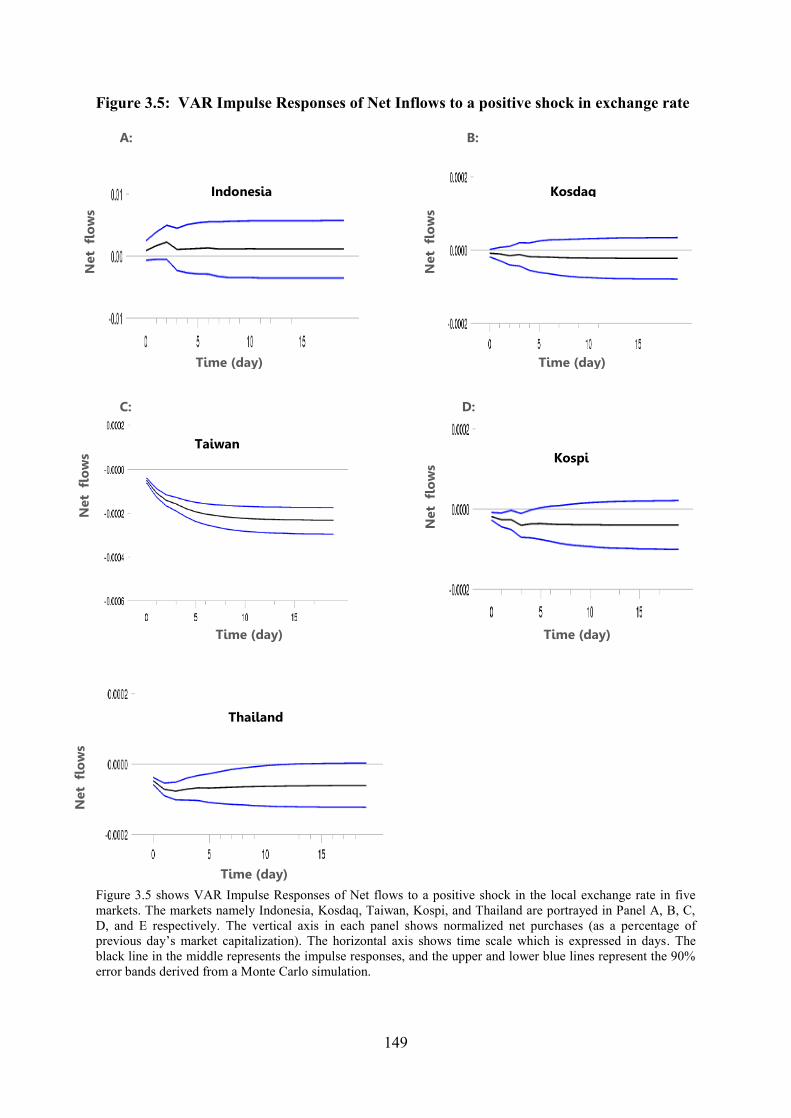
149
Figure 3.5: VAR Impulse Responses of Net Inflows to a positive shock in exchange rate
A: B:
C: D:
Figure 3.5 shows VAR Impulse Responses of Net flows to a positive shock in the local exchange rate in fivemarkets. The markets namely Indonesia, Kosdaq, Taiwan, Kospi, and Thailand are portrayed in Panel A, B, C,D, and E respectively. The vertical axis in each panel shows normalized net purchases (as a percentage ofprevious day’s market capitalization). The horizontal axis shows time scale which is expressed in days. Theblack line in the middle represents the impulse responses, and the upper and lower blue lines represent the 90%error bands derived from a Monte Carlo simulation.
Net
flo
ws
Net
flo
ws
Time (day) Time (day)
Net
flo
ws
Net
flo
ws
Net
flo
ws
Time (day)
Time (day) Time (day)
Thailand
TaiwanKospi
Indonesia Kosdaq

150
3.7.5 The impact of local returns on foreigners’ trading
The main question investigated in this line of research is whether foreign equity flows
are determined by past local returns. In other words, whether foreign investors engage in
positive feedback trading strategies with respect to local return. Therefore, in this sub-section,
our research does not differ from previous studies by examining the relationship between
foreign inflows and local return, since all previous studies, with few exceptions, have already
documented positive feedback trading for foreign investors in emerging markets. The key
contributions of our work regarding the behaviour of foreign investors with respect to local
return will be presented in the following sections. However, since in the following sections
we will investigate the interaction between foreign inflows and local returns, taking the
changing global and local conditions into consideration, it is useful here to examine the
relationship between foreigners’ trading and local returns for the whole sample as a starting
point for our analysis. Thus, in this section we study the response of net purchases of
foreigners to innovations in local returns. The cumulative responses of net purchases to
innovations in local returns are portrayed in figure 3.6. Impulse response functions for net
inflows start at period 1 rather than period 0 as we place the net purchases of foreigners first
in the order which indicates that net purchases of foreigners contemporaneously affect local
returns, but not vice versa. This way, local returns can only affect net purchases with a lag.
When we move to the results we find that in three markets, namely Indonesia,
Thailand and Taiwan, the cumulative responses of net inflows to a one standard deviation
shock in local returns are both positive and statistically significant. In the Kosdaq and Kospi
markets the cumulative responses of net inflows are also positive, but not statistically
significant. However, while in the first three lags for the Kosdaq market and four lags for the

151
Kospi market the cumulative responses are found to be statistically significant, they become
insignificant thereafter, but remain positive out to 20 lags. Since local return affects net
inflows with a one period lag, the biggest impact on net flows can be observed in the first
period with 43%, 67% and 87% of the total impact for Taiwan Indonesia and Thailand
respectively. Since accumulated total impacts of local returns on net inflows decrease after
the first and second periods for Kosdaq and Kospi, respectively, the impacts of local returns
on net inflows in their first periods exceed the total impact. The cumulative responses of net
inflows to a one standard deviation shock in local returns correspond to 0.29%, 0.43%,
0.48%, 0.91% and 0.98% of market capitalization for Kosdaq, Indonesia, Kospi, Thailand
and Taiwan respectively. Given these results it is obvious that a one standard deviation
increase in yesterday’s local returns leads to a relatively large increase in foreign demand in
Taiwan compared to the total supply of available shares in the respective local markets.
It is clear from these estimates that the cumulative median impact of US returns on
net inflows is much higher than the cumulative median impact of local returns on net inflows,
with the estimates of 0.95% versus 0.48% of market capitalization. This finding is similar to
those of Griffin et al (2004) and Richards (2005) who examine foreigners’ trading in
emerging markets on a daily basis. Finally, our results support the notion that foreign
investors are positive feedback traders with respect to local return.

152
Figure 3.6 VAR Impulse Responses of Net Inflows to a Positive Shock in Local Return
A: B:
C: D:
Figure 3.6 shows VAR Impulse Responses of Net flows to a positive shock in local return in five markets. Themarkets namely Indonesia, Kosdaq, Taiwan, Kospi, and Thailand are portrayed in Panel A, B, C, D, and Erespectively. The vertical axis in each panel shows normalized net purchases (as a percentage of previous day’smarket capitalization). The horizontal axis shows time scale which is expressed in days. The black line in themiddle represents the impulse responses, and the upper and lower blue lines represent the 90% error bandsderived from a Monte Carlo simulation.
Net
flo
ws
Net
flo
ws
Time (day) Time (day)
Net
flo
ws
Net
flo
ws
Time (day) Time (day)
Net
flo
ws
Time (day)
IndonesiaKosdaq
TaiwanKospi
Thailand
153
3.7.6 The impact of local returns on foreigners’ trading at different global riskappetite levels
In section 3.8.4, similar to the findings of previous studies we find that foreign
investors follow positive feedback trading strategies with respect to local return. The
contribution of this section lies in being the first attempt to relate foreigners’ trading
strategies to global risk appetite. To this end, we classify levels of global risk appetite as
“high” and “low”. We then estimate our impulse response functions for foreign net flows to a
one standard deviation shock in local return in the high and low risk levels separately. The
hypothesis two is tested by looking at the cumulative impulse responses in these two different
VAR systems in terms of sign and significance criteria in the two different levels of global
risk appetite. As mentioned before, since we are dealing with cumulative impulse responses
in two different systems we do not employ wald tests as is typically employed to determine
whether the coefficients are significantly different in a classical linear regression or in a
system of regressions. With a VAR, we are generally interested in the overall behaviour of
the model rather than in the individual coefficient values, or the significance of individual
coefficients.
We report the cumulative responses of foreign inflows to a shock in local returns in
figure 3.7. Responses in both high and low risk appetite levels are portrayed side by side.
Regarding the hypothesis two, when looking at the impulse response graphs we come up with
interesting results. A first point to mention is that in three out of five markets namely
Indonesia, Kosdaq and Kospi the cumulative responses of foreign inflows to a one standard
deviation shock in local return are different across high and low risk appetite levels. For
example, in Kosdaq, while the cumulative impulse response of foreign inflows is negative
with borderline significance in high levels of global risk appetite, it is found to be positive

154
and statistically significant in low global risk appetite levels. This implies that foreign
investors are positive feedback traders at times when the global risk appetite is low and
negative feedback traders at times when the global risk appetite is high. Given this finding,
the question then arises as to what might be the cause of this behavioural difference in the
Kosdaq market. One explanation is that foreigners use recent local returns as information
signals only at times when they have a low appetite for risk, whereas they use other
information sources as information signals for expected return of the local market at times
when they have a high appetite for risk. The reason for this kind of behaviour can lie in an
ambition to earn money when they have a high appetite for risk. Thus, they may prefer to use
other information sources rather than just chasing recent returns.
Similar responses are also found for foreign inflows in Kospi although they are
insignificant. Since Kosdaq and Kospi are the two stock markets in South Korea, it is not
surprising that we obtain the same behaviours for foreigners in Kospi market. However, when
looking at the case of Indonesia the result is puzzling, because, our finding is just the opposite
behaviour compared to that found in the Kosdaq and Kospi markets. That is to say, the
cumulative impulse responses of foreign inflows to a shock in local returns in Indonesia is
found to be positive, with borderline significance in high risk appetite levels, while it is found
to be negative though insignificant in low risk appetite levels. In other words, foreign
investors act in a contrarian style with respect to local returns when their risk appetite is low
and act in a momentum manner when their risk appetite is high.
One possible explanation for the negative feedback trading in Indonesia when
foreigners are risk averse may result from foreign investors’ perceptions on valuations. When
foreigners are more risk averse they may be more sensitive about pricing the assets and they

155
may have weaker extrapolative expectations for that local market than those they have when
they are less risk averse. That may be why foreigners are positive feedback traders when they
are less risk averse since they have stronger extrapolative expectations for that local market
than those they have when they are more risk averse.
However, in terms of foreign investors, a question still remains as to what makes
Indonesia different from Kospi and Kosdaq. One possible explanation for this difference is
that since Korea market is nearly five times as big as Indonesia’s in terms of market
capitalization global institutional investors can prefer to invest relatively more in Korea
compared to Indonesia, and it is also plausible to believe that global institutional investors
can invest in information sources, thanks to their size, global experience, talent and resources
which renders them to be at an informational advantage relative to locals. Therefore,
foreigners in Korea may not be more sensitive about pricing the local assets when global risk
appetite is low compared to foreign investors in Indonesia. In this scenario, foreigners in
Korea may even have advantages in analyzing push factors, especially at times when
domestic markets are highly influenced by global factors, in other words when the global risk
appetite is high, compared to foreigners in Indonesia.
When we move to the reactions of foreigners following a shock in local returns in the
Taiwan and Thailand markets we find positive cumulative impulse responses for foreign
flows in each market at both risk appetite levels. In Taiwan, both responses are positive with
borderline significance levels, whereas in Thailand despite having positive responses in both
risk appetite levels it is found to be statistically significant only in the low risk appetite level.
Given the above, our results for Thailand and Taiwan demonstrate that foreigners in these
markets use recent local returns as the only information signal. In other words they have

156
extrapolative expectations about the expected returns of the local market irrespective of their
risk tolerance levels.
Figure 3.7 VAR Impulse Responses of Net Inflows to a positive shock in local return atlow and high periods of global risk Appetite.
A LOW GRA B HIGH GRA
Net
flo
ws
Net
flo
ws
Time (day) Time (day)
Net
flo
ws
Net
flo
ws
Time (day) Time (day)
Net
flo
ws
Net
flo
ws
Time (day) Time (day)
Kospi Kospi
KosdaqKosdaq
Indonesia Indonesia

157
Figure (3.7) continued
Panel A and B, in figure 3.7, show VAR impulse responses of net inflows to a positive shock in local return infive markets at low and high periods of global risk appetite respectively. The markets are Indonesia, Kosdaq,Taiwan, Kospi, and Thailand. The vertical axis in each panel shows normalized net purchases (as a percentageof previous day’s market capitalization). The horizontal axis shows time scale which is expressed in days. Theblack line in the middle represents the impulse responses, and the upper and lower blue lines represent the 90%error bands derived from a Monte Carlo simulation.
Net
flo
ws
Net
flo
ws
Time (day) Time (day)
Net
flo
ws
Net
flo
ws
Time (day) Time (day)
ThailandThailand
Taiwan Taiwan

158
3.7.7 The impact of local returns on foreigners’ trading at different states of theeconomy
Having documented that foreign investors engage in positive feedback trading
strategies with respect to local returns, we now look at whether foreigners chase recent local
returns irrespective of economic conditions in the emerging country. To do so, we classify
levels of economic activity as “boom”, “recession” and “normal” periods and we similarly
estimate the response of foreign flows to innovation in local returns in boom and recession
periods. Our interest, in this section, is focused on the trading differences with respect to local
return across two states of the economy. We test the hypothesis three by looking at the
cumulative impulse responses in these two different VAR systems in terms of sign and
significance criteria in the two different states of the economy.
The cumulative impulse response functions of net inflows to a one standard deviation
shock in local returns are shown in figure 3.8. Regarding the hypothesis three, we find that in
two out of five markets namely KOSPI and Thailand the cumulative impulse response
functions for foreign flows are different. For example, in Kospi, while the response is
positive and statistically significant in the low state of the economy it is found to be negative
in the high state of the economy, though insignificant. In Thailand, unlike Kospi, the
cumulative impulse response of foreign flows is negative, but very close to zero, in low states
while it is found to be positive in the high state of the economy, though both cumulative
responses are not statistically significant. It is also worth noting that we find different
responses for foreign flows in the Kosdaq when comparing the responses for the whole
period. The cumulative impulse response of foreign flows to a shock in local returns is found
to be negative in both states of the economy, whereas we find a positive cumulative impulse
response function for foreign flows for the whole period.

159
In the content of Taiwan and Indonesia we find no difference in cumulative impulse
response functions across two states of the economy. In Taiwan, the cumulative responses are
both positive and insignificant in both states of the economy. When we come to Indonesia the
responses are found to be positive in both states of the economy, though a significant
response is found only in the high state of the economy.
To sum up, since we find no significant differences in trading behaviours across states
of the economy, our results can be regarded as evidence that supports the model of Brennan
and Cao (1997). This suggests that foreign investors use recent returns as information signals
for that local market, as they have an informational disadvantage in emerging markets. Our
finding demonstrates that their model works irrespective of local conditions.
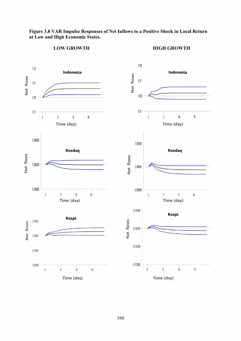
160
Figure 3.8 VAR Impulse Responses of Net Inflows to a Positive Shock in Local Returnat Low and High Economic States.
LOW GROWTH HIGH GROWTH
Figure (3.8) continued
Net
flo
ws
Net
flo
ws
Time (day) Time (day)
Net
flo
ws
Net
flo
ws
Time (day) Time (day)
Net
flo
ws
Net
flo
ws
Time (day) Time (day)
KospiKospi
Kosdaq Kosdaq
Indonesia Indonesia

161
Figure (3.8) continued
Panel A and B, in figure 3.8, show VAR impulse responses of net inflows to a positive shock in local return infive markets at low and high states of the economy respectively. The markets are Indonesia, Kosdaq, Taiwan,Kospi, and Thailand. The vertical axis in each panel shows normalized net purchases (as a percentage ofprevious day’s market capitalization). The horizontal axis shows time scale which is expressed in days. Theblack line in the middle represents the impulse responses, and the upper and lower blue lines represent the 90%error bands derived from a Monte Carlo simulation.
Net
flo
ws
Net
flo
ws
TaiwanTaiwan
Time (day) Time (day)
Net
flo
ws
Net
flo
ws
ThailandThailand
Time (day) Time (day)

162
3.8 Conclusion
This study is the first to investigate the impact of global risk appetite on equity flows
to emerging markets. This issue is of great concern to both academicians and policy makers,
especially given the recent ongoing credit crisis or subprime panic started in the USA which
led to capital outflow from almost every emerging stock market. Taken together, the findings
in this chapter show that global risk appetite is also an important factor, in addition to local
and global returns, that affects net purchases of foreigners in emerging markets. It is not
likely to obtain unbiased estimates of the variables included in the regression in the absence
of global risk appetite. Moreover, two further innovations, in this chapter, suggest different
implications for policy makers at different times, which show the importance of the
innovations we have introduced in terms of regulators in the emerging markets.
Now, when we move to the analysis of foreigners’ trading in a more detailed way we
find that in four out of five markets the cumulative responses of foreign inflows to a one
standard deviation negative shock in the VIX index are positive and significant. In the fifth
(Indonesian) case, the cumulative response is also found to be positive out to 20 lags, but
only significant up to the third lag and becomes insignificant thereafter. The most likely
reason for this difference, which we find most consistent with the data, is that foreigners in
Indonesia are likely to overreact to a negative shock in the global risk appetite, resulting in
high increase in net purchases followed by partial corrections. When looking at the impulse
response graphs we see that subsequent net inflows after the third lag exhibit partial reversals
making the cumulative response insignificant but still positive, which can be regarded as
evidence of partial overreaction.

163
We also examine the effects of US returns on net inflows to emerging markets. In a
similar vein, in four out of five markets the cumulative responses to a positive shock in the
US returns are positive and significant out to 20 lags. In the Indonesian case, while the
cumulative response is positive up to 20 lags, statistical significance is found after the third
lag.
When we move to analysis of foreigners’ trading with respect to local returns we find
that cumulative responses are positive and significant in Indonesia, Thailand and Taiwan
showing that foreigners are positive feedback traders. In Kosdaq and Kospi markets
cumulative responses of foreign inflows are also positive though insignificant. Similar to
previous findings as in Griffin et al (2004) and Richards (2005) we find that the impact of US
returns has much more influence on the trading decisions of foreign investors compared to
the impact of local returns on their trading.
We also include the foreign exchange rate into the VAR system and find some
interesting results. For example, the accumulated effects of a positive shock in the exchange
rate, corresponding to a depreciation of the local currency, are negative in four out of five
markets. In the Kospi and Kosdaq markets the accumulated impacts are not statistically
significant, but in Thailand and Taiwan they are. The results may appear at first glance as
puzzling, but one possible explanation for this response is that in an environment where
foreigners use the exchange rate as a proxy for local macroeconomic fundamentals, and in a
context where a depreciation of the local currency signals negative conditions about the
economy, foreign investors use this as an informational signal and sell their stocks.
As a second innovation, our study also investigates the interaction between foreign
flows and emerging stock market returns, while taking the global risk appetite into

164
consideration. We examine how foreigners behave with respect to local return at different
risk appetite levels. We find different cumulative impulse responses for foreign inflows
across high and low risk appetite levels in Indonesia, Kosdaq and Kospi markets. For
example, we find that foreigners behave in a momentum style with respect to local return at
times when the global risk appetite is low and in a contrarian style when the global risk
appetite is high. Similar behaviour is also found for foreigners in Kospi, although it is
insignificant. A possible explanation for this difference is that foreigners use recent local
returns as information signals only at times when they have a low appetite for risk, whereas
they use other information sources as information signals for expected returns on the local
market at times when they have a high appetite for risk. The reason for this kind of behaviour
can lie in an ambition to earn money when they have a high appetite for risk. Thus, they may
prefer to use other information sources rather than just chasing recent returns.
However, we document completely opposite behaviour for foreigners in Indonesia.
The cumulative impulse response is positive at high risk appetite levels with borderline
significance, whereas it is negative at low risk appetite levels though insignificant. One
possible explanation for the negative feedback trading in Indonesia when foreigners are risk
averse may result from foreign investors’ perception on valuations. When foreigners are more
risk averse they may be more sensitive about pricing the assets and they may have weaker
extrapolative expectations for that local market than those they have when they are less risk
averse. That may be why foreigners are positive feedback traders when they are less risk
averse since they have stronger extrapolative expectations for that local market than those
they have when they are more risk averse.
165
However, in terms of foreign investors, a question still remains as to what makes
Indonesia different from Kospi and Kosdaq markets. One possible explanation for this
difference is that since Korea is nearly five times as big as Indonesia in terms of market
capitalization global institutional investors may prefer to invest more in Korea compared to
Indonesia, and it is also plausible that global institutional investors can invest in information
sources, thanks to their size, global experience, talent and resources which renders them to be
at an informational advantage relative to locals. Therefore, foreigners in Korea may not be
more sensitive about pricing the local assets when global risk appetite is low compared to
foreign investors in Indonesia. In this scenario, foreigners in Korea may even have
advantages in analyzing push factors, especially at times when domestic markets are highly
influenced by global factors, in other words when the global risk appetite is high, compared
to foreigners in Indonesia.
From a policy making point of view our finding about these three markets especially
for Kosdaq is of high relevance for regulators when introducing necessary measures to
enhance stability of the market.
Finally, as a third innovation, when we analyze foreigners’ trading with respect to
local returns under different states of the local economy we find that the cumulative impulse
response of foreign flows to a shock in local returns are different across the two states in
KOSPI and Thailand. In KOSPI the cumulative response is found to be positive and
significant in the low state of the economy, whereas it is negative and very close to zero
though insignificant in the high state of the economy. The responses are found to be opposite
when looking at Thailand. That is to say the cumulative response is found to be negative in
the low state of the economy and positive in the high state of the economy, though both

166
responses are insignificant. At this point, since we find different behaviours in our VAR
model for these two markets it is not likely to support the model of Brennan and Cao (1997)
which suggests that foreign investors use recent returns as information signals about the
expected return of the local market as they have an informational disadvantage in emerging
markets. In contrast, our finding regarding these two markets suggests that foreigners do not
follow positive feedback trading strategies irrespective of local economic conditions.

167
Chapter 4: How Do Different Players in the Stock Market React to MacroeconomicNews?

168
4.1 Introduction
Do foreigners react differently on the announcement of macroeconomic news,
compared to local institutions or private investors? This question should be of great
importance to stock market regulators. It is often argued that foreigners cause large and
unpredictable currency flows and movements in share prices. However, if foreigners react in
the opposite way to locals, then it could be argued that they have a calming effect on the local
market, rather than increasing volatility. Any argument in favor of exchange controls or
limits on foreign shareholdings would then become more difficult to support. This study is
the first empirical research in the literature that looks at the reaction of foreign investors to
local macroeconomic announcements in emerging markets.
According to the Dividend Discount Model, share prices should be based on the sum
of the expected future dividend flows, discounted back to the present. Thus share prices
should be affected by news that is likely to change future dividends or discount rates.
Macroeconomic conditions are a major determinant of these, so it is unsurprising that many
studies have looked at macroeconomic news announcements as a likely source of price
changes (see, for example, McQueen and Roley, 1993, and Flannery and Protopapadakis
2002).
An equally popular area of research has been the trading behavior of different groups
of investors. As Rubinstein (1993) stated, people reading the same news items can come to
different conclusions. Much work in behavioral finance has shown that private investors are
more prone to behavioral biases and more likely to act in a contrarian manner.

169
However, there has been little research into how different groups of market
participants behave when they learn of macroeconomic news announcements. Financial
economists should be greatly concerned with whether players in the stock market react
differently to news announcements, since it is the trading of these market participants that
changes share prices and moves them to new equilibria.
As far as we know, there have only been two studies that have analyzed the
differential impact of macroeconomic news on different groups of investors. Nofsinger
(2001) looked at the reaction of institutional and individual investors around macroeconomic
news releases for NYSE stocks. However, his study aggregated all news announcements, and
only looked at stocks over a three-month period starting from 1 November 1990 and ending
in 31 January 1991.
The only other study we have found is that of Erenburg, Kurov, and Lasser (2006).
They looked at how macroeconomic announcements affect the trading behavior of exchange
locals and off-exchange traders in S&P 500 index futures contracts. They found that local
traders reacted more quickly to macroeconomic news releases than off-exchange traders, i.e.
they bought futures more quickly after good news and sold them more quickly after bad.
However, both studies either have some shortcomings in their methodology or need to
be extended in different aspects. Our study differs from above two studies in the following
ways.

170
First, a potential shortcoming with respect to Nofsinger’s (2001) study is related with
the methodology that the study has used due to having a short sample period. Nofsinger
(2001) implements an aggregated approach by constructing a single dummy variable that
aggregates information for 17 different macroeconomic news releases over 63 days.
Therefore, the question of which macroeconomic news releases (individually) have a
significant effect on (buying or selling) behaviour of different types of investors remains an
unresolved issue. In addition, the second drawback of the study is that it determines whether
the macroeconomic news is good or bad by calculating the adjusted returns. However, in this
way, it is not possible to determine whether a specific macro announcement is good or bad if
it is released concurrently with the other announcements. Therefore, our study addresses
these issues by using forecast data coming from an international economic survey
organization which allows us to calculate surprises and separate the effects of
macroeconomic variables that gets announced simultaneously.
Second, the main shortcoming of the previous studies is that they do not take the
same-day correlation between investors’ purchases and local returns into consideration while
investigating reactions of different types of investors around macroeconomic announcements.
However, previous studies for emerging markets, (e.g., Griffin et al, 2004; Richards, 2005)
have found significant evidence of correlations between net purchases (which can be
considered as investor sentiment) of market participants and contemporaneous local market
returns. Therefore, one could argue that any model not taking this correlation into account is
incomplete since if domestic market returns are influenced by the macroeconomic
announcement releases there is a risk that macroeconomic announcements can be found to
have an effect on net purchases (investor sentiment) of investors, but this might be spurious
due to picking up the correlation between net purchases (investor sentiment) and domestic

171
return. Furthermore, this correlation can also be sourced from possible endogeneity
relationship between investors’ purchases and local return, and if endogeneity is present, it
will not be possible to obtain unbiased and consistent estimates due to the regressor- error
correlation. In such cases, Instrumental variables (IV) or GMM method provide a general
solution in obtaining consistent estimator. Therefore, unlike both studies, the main
distinguishing feature of our paper is that we initially test for the endogeneity of the same-day
returns in these equations in a very detailed way in order to decide whether there is need to
resort to IV or GMM estimation methods. If local returns are found to be endogenous one
should proceed with the IV/GMM methods. However, if it is not found to be endogenous this
time local returns should be included as an exogenous variable in these equations in order to
obtain unbiased estimates of the impact of the macroeconomic news. Therefore, both studies
are incomplete in this sense.
Third, many studies, for emerging markets, have documented significant correlation
between net purchases of investors and other independent variables. For example, Richards
(2005) has found significant evidence of correlation between net purchases of investors and
lagged local market returns and the study has also documented substantial autocorrelation in
net purchases of market participants as well. Thus, unlike methodology of both studies,
lagged net purchases and lagged local returns are used as control variables to obtain unbiased
estimates of the impact of the macroeconomic news.
Fourth, many studies, such as McQueen and Roley (1993) and Li and Hu (1998), have
investigated the response of stock prices over different stages of the business cycle since
investors can consider the same type of news to be bad in some stages of the business cycle
and good in others. Therefore, unlike both studies, we also take different states of the

172
economy into consideration to see whether the reactions of investors to macroeconomic news
are different at different points in the business cycle.
Fifth, unlike both studies, we also take different states of the stock market into
account since investor reaction can be different in bull and bear market periods (see for
example, Hardouvelis and Theodossiou, 2002).
Furthermore, our work is also related to another literature that investigates the trading
behaviour of foreign investors in emerging markets. Our research will also be the first study
in the literature that examines the reaction of foreign investors to local macroeconomic
announcements in emerging markets.
By analyzing the above issues, our study is of certain relevance to academics, since
our results can provide useful insights on market efficiency and price discovery, because,
according to the efficient market theory, at any given time prices should reflect all available
information regarding a particular stock. Only new and unpredictable component of
information is expected to move asset prices. Since unexpected component of
macroeconomic news is used in our study as “news” it enables us to see which type of
investor’s trading behaviour acts as catalysts in the price discovery process or helps to
facilitate to gain market efficiency. This issue is important not only to academicians but also
to regulators especially in terms of obtaining information about foreign investors. The
behaviour of foreigners around macroeconomic announcements in emerging markets has not
been investigated so far in the literature. Therefore, this new findings can shed some light on
the issue about whether they trade on announced public information or completely have non-
fundamental motives.

173
In sum, we seek to determine what types of macroeconomic news cause market
participants to buy and / or sell shares and whether investors have different trading patterns
around macroeconomics news releases in the Stock Exchange of Thailand (SET). The choice
of Thailand is not arbitrary. To our knowledge amongst all emerging markets in the world,
Thailand, Taiwan, and South Korea are the only markets that provide daily detailed trading
data (purchases and sales) for three different types of investors namely; local individuals,
local institutional and foreign investors. However, with respect to foreign investors, during
our observation period, regulations on foreign investment in these markets have changed
frequently. For example, in the beginning of our observation period, the ratio of foreign
ownership limit was 49% for Thailand and 12% for Korea and Taiwan. Although barriers
were gradually coming down in these markets foreign investment was still restricted or
completely closed for certain industries in Korea and Taiwan stock markets. However, in
2001, the SET issued a new trading instrument called NVDR (Non-Voting Depository
Receipt) which allows foreigners to invest more than 49% of the shares with receiving all
financial benefits except for voting rights. Given this flexibility in Thailand stock market, it
enables us to explore the trading patterns of foreign investors more accurately relative to
foreign investors in Korean and Taiwan stock markets.
The rest of the chapter is organized as follows: in section 4.2 we provide a review of
the literature addressing the issues mentioned above and state our hypotheses regarding our
research questions. Sections 4.3 and 4.4 describe the data and methodology employed in this
study respectively. Sections 4.5 and 4.6 present descriptive statistics and results, respectively,
and section 4.7 summarizes main conclusion.

174
4.2 Theoretical background
Academics have long thought that arrival of new information should have significant
effect on asset prices due to the basic premise of efficient market theory (EMT). Therefore,
many studies both theoretical and empirical have investigated the impact of “new
information” on stock prices. The information variable is considered to include both a private
and a public component. With respect to private information, firm-specific news is
considered to be the main source of information that affects stock prices. With respect to
public information, macroeconomic announcements are thought to be excellent candidates by
which public information arrives.
This study examines the trading behaviour of foreigners, local individuals, and local
institutional investors around macroeconomic news releases in the Stock Exchange of
Thailand (SET). Thus, our work has its origins in two different literatures: first, an extensive
literature that investigates the effects of macroeconomic announcements on asset prices.
Second, a growing literature that examines the trading behaviour of different types of
investors. We seek to link these two different literatures by the questions addressed in this
study. Since there are numerous studies in both two literatures we present a brief overview of
some important studies in each literature which we regard as influential to our research
questions. With respect to first literature, it is also useful to note that while a voluminous
literature can be found for the role of scheduled macroeconomic information releases on the
volatility of asset prices in various asset markets we prefer to provide a brief review of some
important papers that focus on mean rather than volatility of returns since this study deals
with mean changes in investor sentiment of each investor group.

175
4.2.1 Empirical literature on market reactions to macroeconomic news
According to the basic assumption of efficient market theory, only new and
unanticipated part of the information can affect asset prices. Failure to distinguish between
expected and unexpected part of the announcement would tend to bias the news effect on
stock prices. Early studies which take this issue into consideration begin with Pearce and
Roley (1985), who use survey expectations data provided by Money Market Services (MMS)
for the expected portion of these macroeconomic announcements, while investigating the
daily response of S&P 500 index to macroeconomic announcements to examine whether the
result supports the efficient market hypothesis. The sample period starts on September 29,
1977, and ends on October 15, 1982. Six macroeconomic announcements (namely narrowly
defined money stock, Consumer Price Index, Producer Price Index, unemployment rate,
industrial production, and Federal Reserve's discount rate) are considered as fundamental
public information signal about the economy. Money announcement surprises are found to
have significant effect on equity prices. The study finds little evidence of association between
stock prices and surprises in both inflation and real activity. Additionally, the study finds that
anticipated portion of the economic announcements have no effect on stock prices that
supports efficient markets view. Jain (1988) extends Pearce and Roley (1985) work by
employing hourly stock returns data for US market to obtain more precise estimates for
equity price responses. The sample period employed in the study begins at the start of 1978
and ends at the close of 1984. Jain (1988) finds that surprises of money supply
announcements have significant negative effects on equity prices. Jain (1988) documents
more strong relationship (high t statistics) for the surprises of money supply announcements
than those of Pearce and Roley (1985) study. Additionally, he finds that inflation related
announcement surprises have significant effect on stock prices which was found to have no

176
effect on equity prices in the study of Pearce and Roley (1985). Hardouvelis (1987)
investigates the responses of four representative equity price indexes (namely the S&P 500
(large companies), the AMEX (small companies), NYSE (financial companies) and Value
Line Index) to 15 macroeconomic announcements with distinguishing monetary news from
nonmonetary news. The study employs two sub periods. The first sub period begins on
October 11, 1979, and ends on October 5, 1982 and the second sub period begins on October
6, 1982 and ends on August 16, 1984. Hardouvelis (1987) finds that equity prices react
primarily to monetary announcements. NYSE Financial index is observed to be the most
sensitive index to monetary announcements among all four stock prices indexes.
Above studies find little evidence of correlation between surprise component of
macroeconomic news and stock prices. In previous studies the response of stock prices is
assumed to be the same over different states of the economy. However investors can
consider the same type of news to be bad in some stages of the business cycle and good in
others, therefore it may not be possible to obtain the unbiased estimates of the impact of the
surprise component since it is expected to bias toward zero. Therefore, McQueen and Roley
(1993) investigate the daily response of S&P 500 to macroeconomic news over different
states of the economy. Response of stock prices is allowed to vary over different stages of the
business cycle to be able to provide unbiased estimator and identify good news and bad news
across different states of the economy. They find that real activity news, which is higher than
expected, is associated with lower stock prices in a strong economy, whereas the same
surprise results in higher stock prices when the economy is weak. Thus, their finding helps to
explain why some macroeconomic news is found to have insignificant effect on stock prices
in previous studies.

177
Similar to McQueen and Roley (1993), Li and Hu (1998) also examine the reactions
of four stock markets (namely, the S&P 500, the Dow Jones Industrial Index, the Russell
1000 and the Russell 2000 Index) to macroeconomic announcements conditional on the state
of the economy. The study finds that the responses of stock market to the same
macroeconomic announcements vary across different states of the economy. Furthermore,
once the response coefficients are allowed to vary across different economic states more
macroeconomic variables are observed to be significant which have received little attention in
earlier studies. The study also investigates whether small firms and large firms react
differently to macroeconomic surprises and find that small caps respond differently to
surprises in a relative set of macroeconomic announcements both in terms of magnitude and
signs. In this sense, recent study of Boyd, Hu, and Jagannathan (2005) that explores the short
run reaction of US stock prices to the arrival of unemployment news between February 1957
and December 2000 also documents that on average, equity prices react positively to an
announcement of rising unemployment when the economy is in an expansion, and negatively
when the economy is in a contraction.
Another study by Flannery and Protopapadakis (2002) looks at this issue in terms of
multifactor asset pricing models. They argue that previous studies may have failed to find
evidence of significant relation between stock prices and some macroeconomic news if the
market response to surprises in economic announcements is time varying. Therefore,
Flannery and Protopapadakis (2002) extend earlier studies by estimating a GARCH model in
which any macroeconomic announcement series is identified as a potential risk factor that
either impacts stock returns or increases conditional volatility of stock returns. The study uses
value-weighted daily return of NYSE- AMEX-NASDAQ indexes and also extensive data set
including 17 macroeconomic announcements. They find that six of the 17 economic

178
announcement surprises have significant effect on either returns or conditional volatility of
returns. Similar to previous studies, Kim and Kow (2005) look at the same issue in Japanese
market. They investigate the effects of announcement releases of 16 macroeconomic
variables on returns and volatility in the stock, debt and foreign exchange markets of Japan.
The study finds that macroeconomic news has significant effect on both return and volatility
of return in all three markets in Japan. The debt market is found to be more sensitive to
macroeconomic news compared to other two markets. Volatility in three financial markets is
found to increase after the release of the announcements. While inflation related news is
found to drive volatilities in foreign exchange and debt market, it is the growth related news
that causes the stock market to react more sensitive.
Empirical research in this field has mostly documented evidences for mature markets.
Few studies examined the effect of economic announcements on markets prices in emerging
countries. Andritzky, Bannister, and Tamirisa (2007) extend the literature by investigating the
impact of economic announcements on emerging bond prices both in terms of level and
volatility for 12 developing countries. The sample period employed in the study begins on
January 5, 1998 and goes through July 15, 2004. To a great extent, the results are found to be
consistent with those documented for mature markets. The study finds no evidence of a
systematic effect of macroeconomic announcements on the level of emerging bond spreads
but they are found to have a significant impact on the volatility of bond spreads.
Announcements in these emerging markets are also documented to have varying effects
depending on their characteristics. Individual macroeconomic announcements are found to
have less effect in relatively more transparent countries.

179
All above studies have used daily data and relatively smaller set of macroeconomic
announcements. The study of Balduzzi, Elton, and Green (2001) adds to the literature by
employing high frequency stock data to examine the effects of 26 macroeconomic
announcements on the prices of U.S Treasury bonds. Intraday price information allows the
study to analyze the impact of economic news on prices of government bonds at very short
intervals which helps to examine how quickly public information is incorporated into bond
prices. Balduzzi et al (2001) find that several economic news releases have significant impact
on the prices of bonds and these impacts vary significantly depending on maturity. The price
adjustment to news releases is found to take place within one minute or less after the release
of economic news. In addition, the study finds that surprises in economic variables have
significant effect on price volatility. Since bid-ask spreads are found to reverse quickly to
their previous normal levels the study suggests that public information is rapidly incorporated
into prices.
Here, it is worth noting that while using intraday data has advantages it has also some
disadvantages. In one sense, while analyzing the prices at very short intervals allows a
researcher to investigate how quickly information is incorporated into prices, in another
sense, investors can also be thought to need some time to process the information for sound
decisions. Therefore, studies having different frequency of data can make complementary
contribution over each other.
Finally, it is clear from the above literature review that work into the impact of
macroeconomic announcements have been confined to stocks and bonds prices. Given the
importance of the investor behaviour differences in determining the asset prices there is

180
clearly a need to examine the impacts of macroeconomic announcements on the behaviour of
market participants.
4.2.2 Literature on trading behaviour of different types of investors
Heterogeneity of agents is accepted as the most plausible explanation for trade in the
economics and finance literature. In most of the early models of trade such as Pfleiderer
(1984), and Kyle (1985), it is assumed that agents have identical interpretation of
information. A notable exception compared to early studies is Rubinstein (1993) who states
that: “In almost all models of economic theory, behavioural differences among consumers are
attributed to differences in preferences or in the information they possess. In real life,
differences in consumer behaviour are often attributed to varying intelligence and ability to
process information. Agents reading the same morning newspapers with the same stock price
lists will interpret the information differently” (p 473). Later on, Kandel and Pearson (1995)
address the issue of whether the assumption that agents have identical interpretations is
appropriate by investigating the relation between trading volume and returns of stocks around
anticipated public announcements in US market. The study finds economically and
statistically positive association between abnormal trading volume and quarterly earnings
announcements even when there is no change in price level. They argue that their finding is
consistent with the view of Rubinstein (1993) that agents have differential interpretations of
public information signals. On the other hand, they assert that it is also inconsistent with
traditional models of trade that assume that agents have homogeneous interpretations.
Another study by Bamber, Barron, and Stober (1999) test the argument, that whether
Kandel and Pearson (1995) findings can be attributed to differential interpretation, by

181
exploring the direct relationship between differential interpretations and trading volume in
the US market (NYSE/AMEX). The sample period employed in the study begins from the
first quarter of 1984 and goes through to the last quarter of 1994. They document direct
evidence that supports Kandel and Pearson’s (1995) argument that trading associated with
small price changes shows investors’ differential interpretation of public information. As a
result, differential interpretation is found to play significant role in speculative trading. This
differential interpretation of investors can be sourced from differences in endowments,
differences in preferences (i.e., risk appetite) or differences in information. Thus, information
announcement is expected to generate price and volume changes due to trading through time
by heterogeneous participants trying to understand beliefs of each other since market
participants try to understand each others’ beliefs while forming their own beliefs. Trading
volume jumps as different market participants rebalance their portfolios in response to their
own beliefs and their perception of others which then leads to changes in the levels to re-
establish equilibrium pricing (Keem and Sheen, 2000). This observed trading volume
persistency occurs after information shocks realizations.
Trading of individual investors is generally thought to be more prone to psychological
bias compared to institutional trading in the behavioural finance literature. Therefore, many
studies began to investigate the reaction of institutional and individual investors separately to
different types of news releases. For example, Lee (1992) investigates intraday volume
reactions around various types of earnings announcements in the NYSE. The sample period
starts on January 4, 1988 and ends on December 30, 1988. Market orders placed less than
$10,000 are assumed as small traders. The study finds that two groups react differently to the
same earnings news when accepting trade size as a credible proxy for distinguishing small
traders from institutional traders. Small traders are found to be net buyers during the periods

182
of earnings announcements irrespective of the sign of the news, whereas institutional traders
involve in intense buying only subsequent to good news.
Hirshleifer et al (2008) examine the trading behaviour of U.S individual investors in
response to extreme surprises in quarterly earnings to see whether it is the source of post-
earnings announcement drift (PEAD). The sample period is January 1991 - December 1996.
They find no evidence that individual investors are the cause of PEAD. Individual investors
are found to be significant net buyers regardless of whether earnings surprises are positive or
negative. Etter et al (1999) investigate the speed in processing of new information for the
case of annual earnings announcements by individual and institutional investors. They use a
sample of non –US and non-Canadian firms that are listed on either NYSE or AMEX for the
period between 1983 and 1992. The study finds that Institutional investors seem to process
new information more rapidly than do individual investors. Yuan (2007) investigates the
impact of market wide attention grabbing events on the trading behaviour of US individual
and institutional investors for the sample period between January 1983 and December 2005.
High attention is found to cause individual investors to decrease their stock holdings
dramatically in good times and modestly increase their stock holdings in bad times.
Malmendier and Shanthikumar (2007) examine the trading reaction of U.S individual
and institutional investors to analysts’ recommendations for the sample period that begins on
October 29, 1993 and ends on December 31, 2002. Individual investors are found to follow
analysts’ recommendations literally. They display a positive abnormal response to both buy
and strong buy analysts’ recommendations and no response to hold recommendations.
Whereas, institutional investors display, a positive abnormal response to strong buy
recommendations, no response to buy recommendations and strong selling reaction to hold

183
recommendations. Schmitz (2007) analyze the reaction of individual investors to corporate
news in the media employing 125 companies in German market for the period between July
1998 and October 2006 and find that they react slightly slower to corporate news compared
to other market participants. Barber and Odean (2008) test the proposition that individual
investors buy only stocks that catch their attentions. They test this proposition for the US
market with the sample period from January 1991 through December 1996. Attention driven
buying behaviour of investors is tested by sorting stocks on attention grabbing events.
Proxies employed for attention grabbing events are stocks abnormal daily trading volume,
previous one day return and whether a firm is in that day’s news. They find that individual
investors exhibit attention driven buying behaviour by using these three proxies, whereas the
study finds no evidence of attention driven buying behaviour for institutional investors.
Another group of studies investigates trading decisions of institutional and individual
investors in different aspects. For example, Odean (1998) tests the disposition effect, the
tendency to sell winners too early and to hold losers too long, labelled by Shefrin and
Statman (1985), for the US market with the data beginning in January 1987 and ending in
December 1993 and finds that individual investors tend to realize their profits from winning
stocks and retain their losers. Genesove and Mayer (2001) document a similar behavioural
pattern, behaving in a loss-aversion fashion, for both individuals (owner-occupants) and
professional investors for the real estate market in USA. Heath, Huddart, and Lang (1999)
also find an evidence of disposition effect on the exercise decisions of employees for stock
options using exercise records of seven companies in the USA between August 2, 1985, and
December 23, 1994. Heisler, J (1994) and Locke and Mann (2000) document the same
evidence for the existence of disposition effect for small investors and professional investors
in the USA respectively. Apart from US markets, Shapira and Venezia (2001) also show that
184
disposition effect also exists among professional investors in Israel besides finding stronger
effect for individual investors for the period that begins on January 1, 1994 and goes through
the end of 1994.
There is also a growing body of research that investigates the relation between past
returns and individual and institutional trades. Badrinath and Wahal (2002) examine the
trading behaviour of 1200 institutions in all NYSE, AMEX NASDAQ firms for the period
between third quarter of 1987 and the third quarter of 1995 and find that institutions tend to
be positive feedback traders when they have new equity positions but negative feedback
traders both when they leave the previous equity positions and make adjustments to existing
holdings. Nofsinger and Sias (1999), investigating the cross-sectional relation between
changes in institutional ownership and equity returns in the US market for the period between
1977 and 1996, find that institutional investors follow momentum trading strategies, and this
momentum trading of institutions is largely found to be limited to small firms. In the study of
Lakonishok, Shleifer, and Vishny (1994) for the NYSE and AMEX market between the end
of April 1963 and end of April 1968 period, individual investors are posited to engage in
irrational momentum trading due to extrapolation of past growths. Jackson (2003)
investigates the behaviour of individual investors in Australia for the period that begins in
September 1991 and goes through December 2002 and finds that individual investors appear
to be contrarian traders at both aggregate market and cross sectional levels. They are also
found to be net buyers of equities with high recent volatility. Griffin, Harris, and Topaloglu
(2003) investigate the cross-sectional relation between individuals and institutions’ trading
and equity returns in Nasdaq 100 securities on both daily and intradaily basis from May 1,
2000 to February 28, 2001. They find a strong contemporaneous relationship between equity
returns and changes in institutional ownership at the daily level. Institutions are largely found

185
to follow past stock returns. The study finds that stocks in the top deciles based on the
previous days’ performance is 23.9% more likely to be purchased by institutions sold by
individuals.
There is also another growing literature that studies the relation between past returns
and foreign investors’ trades in emerging markets. Choe, Kho, and Stulz (1999) examine the
patterns of foreign investor trading in Korea market for the period that begins on November
30, 1996 and goes through the end of 1997 and find that foreign investors pursue momentum
trading and engage in herding before the Korean economic crisis. During the crisis, herding is
decreased and momentum trading by foreign investors is mostly disappeared. Grinblatt and
Keloharju (2000), examining the past return based behaviour of various investor types in
Finland market from December 27, 1994 to the end of December 1996, find that foreigners
tend to follow momentum strategies. The study finds significant relationship between the
sophistication of the investor type and the degree of contrarianism. While less sophisticated
local individuals are found to pursue contrarian strategies more sophisticated local
institutions tend to be momentum investors like foreign investors. Kim and Wei (2002)
investigate the trading patterns of foreign investors in different categories in Korea for the
period beginning on January 1, 1997 and ending on June 30, 1998. They find that foreigners
outside Korea are more likely to pursue momentum trading strategies and are more likely to
exhibit herding behaviour than the foreigners living in Korea. Dahlquist and Robertson
(2004) study the behaviour of foreign investors in Swedish market for the 1993 to 1998
period and find that foreign investors act as uninformed positive feedback traders. Griffin,
Nardari, and Stulz (2004) examine the equity flows (net purchase of foreign investors) to nine
emerging countries and find that foreigners tend to be momentum traders in these local
markets. Richards (2005) investigates the trading behaviour of foreign and domestic investors

186
in six Asian markets in the period January 1999 to September 2002. Foreign investors are
found to be positive feedback traders and local individuals appear to be contrarian traders.
Finally, apart from above studies, two studies investigate the reaction of investors
around macroeconomic news releases. The first study by Nofsinger (2001) examines the
trading behaviour of institutional and individual investors around macroeconomic and firm-
specific announcements for NYSE stocks. In this study, in terms of specific news, local
individuals are found to sell on good news rather than bad news which is in line with the
disposition effect. Unlike individual investors, institutions are found to buy and sell following
both good and bad news. In terms of macroeconomic news releases, although both
Individuals and institutions are found to increase their purchases subsequent to good
economic news, individuals are documented to have higher purchase rates compared to
institutions. In terms of selling behaviour, institutions are found to make significantly high
level of purchases during bad economic news, whereas individuals are not found to have
significantly high sales. The second study by Erenburg et al (2006) investigates the effect of
major macroeconomic announcements on the S&P 500 index futures. The study identifies
trader types as exchange local traders and off-exchange traders. Local traders are found to
react to macroeconomic news releases faster than off-exchange traders. That is they are found
to buy (sell) futures following good (bad) news faster than off-exchange traders. The study
also documents profitable strategy for local traders compared to off-exchange traders.
To sum up, only two papers have investigated the behaviour of investors around
macroeconomic announcements. However, both papers have not produced conclusive
evidence due to potential shortcomings in their methodology and also both studies need to be
extended in different aspects as well.

187
4.2. 3 Shortcomings of previous studies and motivation
In view of the two different literatures given above, it is rather surprising to note that
very little attention has been devoted to the analysis of investor behaviour around
macroeconomic news releases. To the best of our knowledge the only studies that we know of
that try to analyze the effect of macroeconomic news on different types of investors are the
ones of Nofsinger (2001) and Erenburg et al (2006) for NYSE stock market and Index futures
market of USA, respectively. However, since these two studies either have potential
drawbacks or need an extension in their methodologies they fall short of our goals in one way
or another.
For example, one potential drawback in Nofsinger (2001) study is the methodology
the study uses in investigating the reaction of institutional and individual investors around
macroeconomic news releases for NYSE stocks. The study uses a single dummy variable that
contains information from 17 different macroeconomic variables over 63 days. Therefore, it
is not possible to isolate the individual effect of specific macroeconomic announcement on
the behaviour of different types of investors. Since we employ forecast data about each
macroeconomic variable coming from an international economic survey organization our
methodology allows us to capture the effect of each macroeconomic announcement on the
trading behaviour of investors.
Another point that our research diverges from both studies is that both studies do not
take potential endogeneity issue (resulted from the mutual dependence of local returns and
investors’ purchases) into account while investigating the reaction of investors around
macroeconomic announcements. However, this may lead to biased coefficients due to the

188
potential same day correlation between foreigners’ purchases and local returns. In addition,
we also take different states of the economy into account in our study since the reactions of
investors to macroeconomic announcements can be different at different states of the
economy (see for example, McQueen and Roley, 1993). Similarly, we also take different
states of the stock market into account since behaviour of investors can change during bull
and bear market periods (Hardouvelis and Theodossiou, 2002). Finally, our work will also be
the first to study the behaviour of foreign investors around macroeconomic news in an
emerging country.
To sum up, given the above literature review and shortcomings of previous studies,
this chapter presents these important issues with their stated hypotheses.
This study will analyze aforementioned research questions such as how local
individual, local institutional and foreign investors behave (buy and / or sell shares in the
Stock Exchange of Thailand) around macroeconomic announcements and whether the
reactions of these investors to macroeconomic news are consistent with the stylized facts
documented regarding the behaviour of different types of investors in the literature. For
example, as mentioned in the literature review, a great deal of empirical evidence shows that
foreign and institutional investors exhibit momentum investment style, whereas individual
investors follow contrarian investment style with respect to past returns (see, e.g., Grinblat
and Keloharju, 2000, Kim and Wei, 2002, Dahlquist and Robertson, 2004, Griffin, Nardari,
and Stulz, 2004, and Richard 2005). In this context, momentum (contrarian) behaviour can be
translated into a tendency to buy (sell) stocks after positive news and sell (buy) stocks after
negative news around the macroeconomic announcement (Vieru, Perttunen, and Schadewitz,
2006).

189
Given the above, the behaviours with respect to macroeconomic announcements can
be formally stated as hypotheses as follows:
Hypothesis (1a): Local individuals sell on good macroeconomic news and buy on bad
macroeconomic news.
Hypothesis (1b): Local institutions sell on bad macroeconomic news and buy on good
macroeconomic news.
Hypothesis (1c): Foreign investors sell on bad macroeconomic news and buy on good
macroeconomic news.
While testing above hypotheses, the state of the economy can also be of certain
relevance to investors. Macroeconomic announcements affect asset prices if announcement
has new information that impacts discount rates or future dividend expectations. However,
the same type of news can be considered bad in some states and good in other states. For
example, McQueen and Roley (1993) find that an unexpected increase in industrial
production leads to a decline in stock prices in high state of the economy due to fears of an
overheating economy. In contrast, the study documents a different sign for the response
coefficient on the same macroeconomic news in the low state of the economy. Similarly,
while an unexpected decrease in unemployment is found to decrease stock prices in high state
of the economy, the study documents an increase in stock price for the same news in low
state of the economy.
For the reasons stated above, it would be useful to investigate whether investors tend
to exhibit same type of trading behaviours around macroeconomic announcements over
different states of the economy.

190
Given the above, the hypotheses can also be stated as below:
Hypothesis (2a): The behaviours of Local individual investors around macroeconomic
announcements are not same across different states of the economy.
Hypothesis (2b): The behaviours of Local institutional investors around macroeconomic
announcements are not same across different states of the economy
Hypothesis (2c): The behaviours of foreign investors around macroeconomic announcements
are not same across different states of the economy
Many studies have investigated the empirical link between investor reaction and the
recent direction of the stock market. For example, Goldberg and Vora (1981) find evidence of
stock return variation with the direction of stock market returns. Klein and Rosenfeld (1987)
document divergent results for the identical events during bull and bear markets. Bowman,
Robin, and Weintrop (1995) also find that recent underlying market conditions (bull/bear
markets) have influence on the event study results. In a more recent study, Docking and
Koch (2005) find that investors perceive good (bad) news as better (worse) news when the
recent direction of the stock market is down (up) and volatile. Given this finding, it would be
useful to investigate whether investors tend to exhibit the same type of trading behaviours
around macroeconomic announcements over different conditions of the stock market.
In view of the above, related hypotheses can be stated as below with respect to first
set of hypotheses regarding the momentum/contrarian investment style;
Hypothesis (3a): The behaviours of Local individual investors around macroeconomic
announcements are not same across bull and bear markets.
Hypothesis (3b): The behaviours of Local institutional investors around macroeconomic

191
announcements are not same across bull and bear markets.
Hypothesis (3c): The behaviours of foreign investors around macroeconomic announcements
are not same across bull and bear markets.
In principle, investors are expected to learn from their trading experiences which, in
turn, improve their trading skills. In this respect, one can argue that if investors lose money
by following momentum or contrarian strategies their trading pattern should not exist
persistently. However, this may not be the case due to two psychological biases, namely
investor overconfidence and self-attribution bias. Overconfident investors are the people who
overestimate their ability and who believe that they have superior ability than others at
choosing the best stocks. Those people, in general, have a tendency to attribute favorable
outcomes to their ability and unfavorable outcomes to external factors. This phenomenon is
known as self-attribution bias which hinders investors learning from their trading experiences
even if they lose money (Gervais and Odean, 2001). In view of the above, one could argue
that during our sample period there was a pervasive financial crisis in Pacific-Asia region
which could have changed the trading behaviour of investors. Therefore, as a robustness
check, it would be useful to investigate whether investors change their trading behaviours
after the crisis compared to pre-crisis period.
Given the above, related hypotheses can be stated as below:
Hypothesis (4a): The behaviours of Local individual investors around macroeconomic
announcements are not same across pre and post crisis periods.
Hypothesis (4b): The behaviours of Local institutional investors around macroeconomic
announcements are not same across pre and post crisis periods
Hypothesis (4c): The behaviours of foreign investors around macroeconomic announcements

192
are not same across pre and post crisis periods.
It is worth mentioning that hypothesis one is the main hypothesis that will be analyzed
throughout the study. In all sub-periods mentioned above, investor sentiment will be analyzed
with respect to the hypothesis one in addition to Wald tests that test for whether their
sentiment changes across sub-periods.
In a nutshell, our research makes the following contributions:
- The first study that investigates the behaviour of investors around macroeconomic
announcements taking into account the endogeneity issue (contemporaneous mutually
dependence of local return and investors sentiment).
- The first study in the literature that examines the reaction of foreign investors to local
macroeconomic news releases in emerging markets
- The first study in the literature investigating the reaction of different type of investors
to macroeconomic news releases that takes the states of the economy into
consideration.
- The first study in the literature that explores the behaviour of different types of
investors around macroeconomic announcements during bull and bear market periods.
4.3 Data
In order to investigate trading behaviour of investors in more detail there is clearly a
need for actual trading data. This study employs daily purchases and sales values for local
individuals, local institutions and foreign investors in Stock Exchange of Thailand (SET)
which allows us to test our hypotheses presented in section 4.2. There are three main investor
groups trading in the SET:

193
1. Local Individuals
2. Local Institutions
3. Foreign Investors
Daily purchases and sales values for local individuals, local institutions and foreign
investors are obtained from the SET. In our data set foreign investors are not divided into
individual and institutional parts. Our data start in February 1995 through May 2008. The
beginning of our sample is dictated by the availability of the investor transaction data. The
nature of our data allows us to examine the reaction of different types of investors to
macroeconomic announcements on a daily basis. On the one hand, using intraday data is not
consistent with the thought that investors need some time to process information for making
sound decision. On the other hand, using monthly or quarterly data might lead to a problem in
differentiating the impact of macroeconomic information from other information. Therefore,
our daily data are long enough to process the information for making decisions and are short
enough to differentiate the impact of economic information from other information.
The motivation of this study is to examine how different types of investors react to
macroeconomic news releases. In order to investigate this relationship, we need a proxy for
investor reaction as the dependent variable and news surprises proxies for the independent
variables. In this line of research, previous studies (eg., Lee, 1992, and Nofsinger 2001) have
developed some measures which are derived from actual trades of investors to capture their
behaviours during news releases. One of these measures which is called “buy-sell imbalance”
is as follows:

194
(1))()(
i,ti,t
i,ti,ti,t sellbuy
sellbuyBSI
Where, BSIit refers to “buy-sell imbalance” and buyit / sellit denote the total value of
shares (in local currency) purchased/sold by investor class i during day t. This measure, BSI,
is also used in the asset pricing literature (e.g., in Kumar and Lee, 2006 as a proxy for
investor sentiment). Therefore, we similarly employ this measure as a proxy for investor
sentiment while investigating the reaction of investors around macroeconomic news releases.
Another measure of BSI, which Lee (1992) named “abnormal order imbalance,
(ABSI), is also used in some studies such as Nofsinger (2001) and Vieru, Perttunen and
Schadewitz (2006) to investigate whether investors buy or sell shares more than usual around
news releases. This measure is defined as:
),BSI(EBSIABSI Where (.)E refers to expectation operator which is the time series
average of BSI in the pre-event period. For example, Vieru et al (2006) use 57 trading days
(t=-60,…-4) as the average (BSI) for the pre-event period while examining whether investors
behaviour on announcement days, (t = 0) differ from the pre-event period. However,
employing this measure as a proxy for investor reaction has some drawbacks in terms of the
information content, because, this measure as a proxy for investor reaction may not capture
the true response of investors around news releases due to the fact that investor sentiment
may have different trends during our observation period. It is these trends which our study
mainly wishes to investigate how investor sentiment changes relative to normal periods. For
example, many studies (e.g., Mc Queen and Roley, 1993; Adams, McQueen and Wood,
2004) document a different stock return response to the same macroeconomic news in
different state of the economy. In a similar vein, previous studies such as Goldberg and Vora

195
(1981), Klein and Rosenfeld (1987) and Weintrop (1995) also document different results for
the identical news during bull and bear markets. Furthermore, Pacific-Asia region
experienced a severe financial crisis during our observation period which could have altered
investor sentiment. Therefore, it may not be possible to examine how investors react to
macroeconomic news across different states of the economy or across different states of the
stock market. It may not be possible to compare how investor behave around macroeconomic
news releases across pre and post crisis periods either since the abnormal measure of BSI
cleans out these trends by subtracting the E (BSI) from BSI. Therefore, to sum up, we employ
BSI measure as was employed in Kumar and Lee (2006) rather than ABSI measure as a
proxy for investor sentiment.
For local market returns, we use SET Price index obtained from Datastream that
includes all common stocks listed on the Stock Exchange of Thailand. Local market returns
are computed by taking first difference of the logged daily SET price index that is readjusted
for stocks dividends. Trading on the SET is order-driven and fully computerized and opening
and closing prices are determined via call auctions in the SET.
There are currently 525 companies listed on the SET. Our sample begins with 389
companies as of January 1995 and reached 525 in May 2008. Table 4.1 shows the annual
number of stocks listed on the stock exchange of Thailand (SET) at the end of each year from
1995 to 2008. We include all stocks that have traded through our sample period. Stocks that
are now dead were included when they were alive.

196
Table 4.1: Annual number of stocks listed in SET
Year number of companies
1994 3891995 4161996 4541997 4311998 4181999 3922000 3812001 3852002 3982003 4202004 4632005 5042006 5182007 5232008 525
This table shows the annual number of stocks listed on the stock exchange of Thailand (SET) at the end of eachyear from 1995 to 2008.
We consider three scheduled macroeconomic announcements in our analysis (namely
industrial production, consumer prices, and trade balance) which we think are representative
of different aspects of the Thailand economy. Two of these announcements i.e. consumer
prices and trade balance are also studied in Wongswan (2006) as important macroeconomic
factors while analyzing the transmission of information originating from USA and Japan to
Thai and Korea stock markets. Besides these two factors we also include industrial
production as it is generally thought to be the most important indicator about economic
activity for any economy. Actual announcements are obtained from the government agencies
that published them. Sources of each announcement are given in table 4.2. For the anticipated
portion of these macroeconomic announcements we prefer to use survey expectations as in
most of the studies in this line of research rather than utilizing econometric estimates as
survey expectations are believed more accurately to reflect contemporary market sentiment
due to containing more recent information. Survey forecasts are also documented to be

197
unbiased and efficient compared to econometric estimates in many studies such as Pearce and
Roley (1985) and McQueen and Roley (1993). Therefore, most of the studies investigating
the impact of economic announcements commonly use survey data such as Ederington and
Lee (1993), McQueen and Roley (1993), Li and Hu (1998), Balduzzi et al (2001), Flannery
and Protopapadakis (2002) Beber and Brandt (2005) and Andritzky et al (2007).
Our expectation data comes from international economic survey organization called
“Consensus economics” that polls more than 180 prominent forecasters each month to obtain
their view and forecasts about the Asian economies. http://www.consensuseconomics.com
Median of analysts’ expectations about each macroeconomic variable is used as a measure of
the market’s expected value for that particular announcement. In this line of research, median
value is commonly preferred in place of mean value since market expectations may not be
represented truly in the existence of extreme values. We calculate “surprises” in
macroeconomic announcements by the difference between the actual data and the median of
analysts’ expectations. Since most of the economic variables have different units of
measurement, we employ standardized surprises of these macroeconomic announcements
while comparing the responses to different macroeconomic announcements. Standardization
is achieved by dividing the surprises by the standard deviation of each announcement
surprises across the sample as was done in Balduzzi et al (2001).
(2)i,t
i,ti,ti,t σ
AFE
Where, tiE , denotes the standardized surprise of announcement i, tiF , and tiA , denote the
median of the forecast survey and the actual released value for announcement i respectively.

198
This does not affect the explanatory power of the model or the statistical significance of the
estimated effects. On the contrary, by providing meaningful deflators it facilitates to compare
the quantitative importance of the estimated responses since a unit variance is guaranteed for
all surprises of the macroeconomic variables. The expectations of Consensus Economics,
Asia Pacific Consensus Forecasts, are made on a monthly basis but are reported as a year-on-
year growth rate. We follow Wongswan (2003) methodology and assumption to convert year-
on-year growth rate expectations to monthly expectations. Details of the conversion
methodology and related unbiased and efficiency tests can be found in appendix A4.1.
4.4 METHODOLGY
4.4.1 Reaction to economic announcements
Regarding the hypothesis one, we investigate whether investors have a tendency to
buy/sell stocks after positive/negative news with respect to their documented trading
strategies in the literature. Although our sample period covers roughly 13.5 years, how
market participants react to news is estimated only for 317 days on which an announcement
is made. In other words our base line equation is the conditional mean equation of BSI
measure (which is used as a proxy for investor sentiment or investor reaction) conditioned on
days on which an announcement is released. There may also be more than one announcement
on some days. Our study is inspired by the seminal works of Mc Queen and Roley (1993),
who examine the reaction of stock returns to macroeconomic announcements and Nofsinger
(2001) who investigates the trading behaviour of individuals and institutions around news
releases. Since our work has its origins in two different literatures we accommodate their
models by the following specification. In this specification, we have investor reaction or

199
investor sentiment proxy as the dependent variable and macroeconomic news surprises
proxies as the independent variables for each investor type.
(3)tutit eIS bx
Where,
itIS = investor reaction or investor sentiment (proxied by “buy-sell imbalance” measure) of
investor group i on that particular day t (the day on which an announcement is made).
utx 1x3 vector of unexpected (surprise) components of economic announcements (Inflation,
Industrial production and trade balance) calculated as the standardized difference between the
actual announcement values and the median value of analysts’ expectations.
et = error term, α is a scalar and b is vector of coefficients.
4.4.1.1 Preliminary analysis
In this section, we try to augment equation (3) with several potential independent
variables as a control variable to obtain unbiased estimates of the impact of the
macroeconomic news. On this basis, we begin with the day of the week effect since trading
volume of different types of investors may be different on different day of the week. For
example, Kallunki and Martikainen (1997) examine the behaviour of small and large
investors in different days of the week for the stock market of Finland. In the study, while
small investors are found to be more willing to sell in the beginning of the week big investors
are found to increase their buy orders. In view of this, we also examine whether
macroeconomic announcements in Thailand are clustered on certain days of the week which
can be seen in table 4.2.

200
Table 4.2 shows the total number of announcements, their respective start dates and
end dates, the total number of announcements released on each day of the week and the
sources of each announcement. All announcements, Consumer Price Index (CPI), Industrial
Production Index (IPI) and Trade Balance (TB), are made on a monthly basis and released
when the market is open. When we look at the table we see that the number of inflation
announcements for each day is quite similar for Tuesday through Friday within the range of
22-30, whereas the number increases to 59 for Monday. The numbers of industrial production
and trade balance announcements, they are released at the same time, have a little bit reversal
pattern. They are very similar for Monday through Thursday within the range of 22-27.
However, the numbers increase to 69 for Friday. We also test for the equality of means for all
announcements across the days of the week and find that the null hypothesis that all
weekdays have equal means is strongly rejected at the 0.00001 level which can be seen in
table 4.2. These results strongly suggest the modification of specification (3) with the day of
the week effect observed in Thailand market. Therefore, we augment our specification with
the day of the week effect as below:
(4)tutit eIS dbx
Where, d = 1 x 4 vector of day-of-the-week dummy variables for Monday through Thursday.
All the other variables and coefficients are defined similarly as in equation (3).

201
Table 4.2: Macroeconomic Announcements (Actual Announcements)
Announcement No of Ann Start Date End Date Monday Tuesday Wednesday Thursday Friday Source
Consumer Price Index (CPI) 160 01/02/1995 02/05/2008 59 30 27 22 22 MoC
Industrial Production Index (IPI) 159 28/02/1995 30/04/2008 20 21 27 22 69 BoT
Trade Balance (TB) 159 28/02/1995 30/04/2008 20 21 27 22 69 BoT
Null hypothesis: fridaythursdaywendesdaytuesdaymonday
F test :Prob : 0.0001***
The table shows the total number of announcements, start and end dates, day distribution, and the sources of each announcement. Source is the reporting agency whereNESDB represents the National Economic and Social Development Board. MoC represents Ministry of Commerce. BoT represents bank of Thailand. CPI, IPI, and TBannouncements are made on a monthly basis. The table also shows the test for the equality of means for all announcements across the days of the week with related F test andProbability values. Null hypothesis is that all week days have equal means. *** indicates significance at the 1 percent level.

202
Furthermore, it can be argued that our results could be driven by the correlation
between net purchases of investors and other independent variables that are not included in
our specification. For example, previous studies, for emerging markets, have found
significant evidence of correlations between foreigners’ purchases and lagged local market
returns and between foreigners’ purchases and lagged mature market returns. These studies
have also documented substantial positive autocorrelations in daily net purchases of foreign
investors as well. In preliminary analysis, the first two lags of net purchases of each investor
type are found to be significant in each equation. Similarly, previous day local market return
is also found to be significant in each equation while the previous day S&P 500 index return
is not. Therefore, unlike the studies of Nofsinger (2001) and Errenburg et al (2006), the first
two two lags of net purchases of investor group i and previous day local market return are
included as control variables so as to account for the movement in net purchases of investors.
Therefore, we augment our specification (4) with our control variables as below:
(5)ttutit eIS cybx
Where, y = 1x3 vector of variables (the first two lags of net purchases of investor group i and
previous day local market return) and c is vector of coefficients. All the other variables and
coefficients are defined similarly as in equation (4). A point worth clarifying here is that after
including three control variables none of the week days are found to be significant in any
equation. Therefore, they are excluded from the equations.
In addition to this, one could argue that our model is still incomplete in the sense that
investor sentiment and contemporaneous local market return can be correlated. Because,
previous studies for emerging markets (for example Richards, 2005) have found significant

203
evidence of correlations between net purchases (can be thought as investor sentiment) of
foreign investors and contemporaneous local market return. Therefore, if domestic market
returns are influenced by the macroeconomic announcement releases there is a risk that
macroeconomic announcements can be found to have effect on investor sentiment but this
might be spurious due to picking up the correlation between investor sentiment and domestic
returns. On this basis, we perform correlation analysis, as shown in table 4.3, to see whether
there is any correlation between different types of investors’ sentiment and same day local
returns.
Results in table 4.3 appear to be consistent with what is documented in the literature.
In other words, it is reasonable to include same-day return as a control variable in order to
avoid possible spurious correlation between investor reaction and macroeconomic
announcements. However, it is also likely to have a suspicion about whether the reactions
(proxied by “buy-sell imbalance”) of foreign investors and local individuals are
endogeneously related with the same day local returns. So, if endogeneity is present, it will
not be possible to obtain unbiased and consistent OLS estimates due to the regressor- error
correlation. In such cases, Instrumental variables (IV) or GMM method provides a general
solution in obtaining consistent estimator.
Table 4.3 Correlations Between Investor Sentiment and Same Day Local ReturnSame day local return
Foreign investors 0.37Local Institutions 0.015Local Individuals -0.40
This table shows the correlations between investor sentiment and same day local return in the SET for the period01/02/1995 – 30/04/2008.

204
In this setup, the information about the movements in explanatory variable (here, the
same-day returns) that is not correlated with the error term is gleaned from one or more
observable variables, called instrumental variables. However, the use of IV or GMM does
come with a price. Because, if the OLS estimator is unbiased and consistent it is inevitable to
lose efficiency when turning to IV or GMM estimation methods (Wooldridge 2003). It is
therefore very important to test for the endogeneity of the same-day returns in these equations
in order to decide whether there is a need to resort to IV or GMM estimation methods. To test
the endogeneity of local returns, we have to find a set of instrumental variables. The choice of
the suitable instruments is an important step. A valid instrument must satisfy two conditions.
First it must be correlated with the explanatory variable (same-day returns) that is causing the
problem known as instrument relevance. Second, it must be uncorrelated with the error term
known as instrument exogeneity. The instrument relevance is very crucial because if the
instruments are not correlated with the endogeneous regressors the IV estimator will suffer
from the same bias as that of OLS estimator. Another serious problem can also appear when
the instruments explain little variation in explanatory variable –which are called as weak
instruments- due to suffering from finite sample bias problems (Baum 2007). Similar to the
instrument relevance, instrument exogeneity is also a very important concept in IV
regression. In the case of single endogeneous variable, as in our case, when we have one
instrument the model is said to be exactly identified and it is not possible to test whether the
instrument is exogeneous. On the other hand, when the number of instrument is greater than
one, M, >1 the model is said to be overidentified and this time it is possible to test the M-1
overidentifying restrictions which provides information about the validity of the instruments.
Before searching candidate instruments for this purpose one has to know some
specialized terminology regarding the definitions of endogeneity and exogenity. For example,

205
in traditional usage in economics, a variable is endogeneous if it is determined within the
model and is exogeneous if it is determined outside the model. On this basis, we are inspired
by Richards (2005) which investigates the trading behaviour of foreign investors in six
pacific countries. In explaining local returns in emerging markets, the study uses same-day
returns of other countries in the same region as explanatory variables. The intuition is that
there may be some unobserved factors that affect all returns in the region. On this basis,
initially, the market returns in the same region can be thought as appropriate instruments for
local return in Thailand. For this purpose, the returns that we think of are as follows: Korea,
Indonesia, Taiwan, Philippines, Hon Kong, Japan, Australian and Singapore. In this scenario,
in terms of economics terminology, it is very reasonable to think of these market returns as
instruments because the returns in these markets are not expected to be determined by the
volume (net purchases of different types of investors) in the Thailand market. In other words,
since these are different markets, they are not expected to be determined in the context of our
model. However, in econometrics terminology, while related to this traditional definition, a
variable is said to be “endogeneous” if it is correlated with the error term and said to be
“exogeneous” if it is uncorrelated with the error term which can be determined by testing
overidentfying restrictions in this respect. However, as mentioned in Wooldridge (2002),
many authors such as Tauchen (1986), Altonji and Segal (1996), and Ziliak (1997) show that
using many overidentifying restrictions is not recommended due to rendering GMM
estimators to have very poor finite sample properties. Therefore, we prefer to choose three
markets out of eight (after preliminary tests), namely Taiwan, Indonesia and Singapore which
are found to have more strong correlations with the Thailand market returns compared to
others and which passed the first stage regression F statistic (will be mentioned later) with the
higher number.

206
After having determined the set of instruments to employ, a point worth mentioning
here is that the standard diagnostic tests for instrument relevance, instrument exogeneity
(overidentifying restrictions) and endogeneity are not valid in the presence of non iid errors in
IV regression. For example, the common approach when faced with unknown form
heterogeneity is to use Generalized Method of Moments (GMM) rather than IV since it is
more efficient. However in the presence of homoskedastic errors IV is preferable to GMM. It
is therefore important to check heteroskedasticity in the IV regression residuals to decide
whether to employ IV or GMM.
As mentioned in Baum (2003) that the standard tests such as Breusch-
Pagan/Godfrey/Cook- Weisberg and White/Koenker to detect heteroskedasticity in an OLS
regression can be valid tests in an IV regression only in the presence of heteroskedasticity in
that equation and nowhere else in the system. This requirement is relaxed in Pagan and Hall
(1983) test statistic which is designed specifically to detect heteroskedasticity in an IV
regression irrespective of the presence of heteroskedasticity elsewhere in the system. Given
the above, we perform Pagan-Hall test, as shown below in table 4.4, to see whether there is
heteroskedasticity in the residuals of IV regressions. 19
In table 4.4 it is seen that whether the disturbance is assumed to be normally
distributed or not doesn’t make any difference and in both test statistics we fail to reject the
null hypotheses that the errors are homoskedastic for both local individuals and foreigners.
Thus, we proceed with IV rather than GMM.
19 Here, it is also useful to note that since there is no correlation between local returns and the reaction of localinstitutions around macroeconomic announcements IV regression is not used for local institution regression.Therefore, Hausman endogeneity test and all other preliminary tests are reported only for local individuals andforeign investors.

207
Table 4.4 Heteroskedasticity test in the IV regression
IV Heteroskedasticity testHo: Disturbance is homoskedastic
Foreign investors
Pagan Hall general test statistic : 8.623 Chi-sq(9) P-value = 0.4728Pagan-Hall test w/assumed normality: 10.89 Chi-sq(9) P-value = 0.2828
Local individuals
Pagan Hall general test statistic: 5.371 Chi-sq(9) P-value = 0.8008Pagan-Hall test w/assumed normality: 9.259 Chi-sq(9) P-value = 0.4137
This table shows the results of heteroskedasticity test in the IV regression for foreign investors and localindividuals. The pagan hall statistic is distributed as χ2 with p degrees of freedom under the null hypothesis thatthe disturbances are homoskedastic irrespective of the presence of heteroskedasticity elsewhere in the system.The test statistic is also reported under the maintained hypothesis that the disturbances are normally distributed.
Similarly, we also check for serial independence in the residuals of IV regression to
see whether there is need to proceed with IV estimator that is robust to autocorrelation.
Similar to the heteroskedasticity tests, the standard tests for detecting autocorrelation such as
the Box-Pierce test, Breusch-Godfrey test and the Durbin’s h test are not valid in the presence
of endogeneous regressors. We follow Baum (2007) suggestion and employ the Cumby–
Huizinga test, as shown below in table 4.5, which is specifically designed to test
autocorrelation in an IV regression.
When looking at table 4.5, we see that the null hypothesis that the residuals are
nonautocorrelated is not rejected for foreign investors. However, we can reject the same null
hypothesis for local individuals at order 1…4 at the conventional 0.05 significance level.
Thus, it is clear that we have to use auotocorrelation robust IV estimator for local individuals.

208
Table 4.5: Cumby-Huizinga autocorrelation test in IVForeign investors
H0: errors nonautocorrelated at order 1..4Test statistic: 3.806 Under H0, Chi-sq(4) with p-value: .432
H0: errors nonautocorrelated at order 1..8Test statistic: 4.721 Under H0, Chi-sq(8) with p-value: .786
----------------------------------------------------------------------------------------------------------------
Local individuals
H0: errors nonautocorrelated at order 1..4Test statistic: 11.555 Under H0, Chi-sq(4) with p-value: .0209
H0: errors nonautocorrelated at order 1..8Test statistic: 14.735 Under H0, Chi-sq(8) with p-value: .0644
This table shows the results of Cumby-Huizinga test in the IV regression for foreign investors and localindividuals. The test statistic is distributed as χ2 with s degrees of freedom under the null hypothesis that theerrors are not correlated for lags q – (q+s). s denotes the number of lag orders to be tested and q denotes thelowest lag order to be tested.
Now, we can move to the diagnostic tests for instrument relevance, instrument
exogeneity and endogeneity for same-day return in the foreigners and local individuals
equations.
Table 4.6 below reports the results for foreigners and individuals equations in part A
and part B, respectively, obtained from Stata. When estimating IV regression in Stata with
enhanced routines it automatically reports underidentification test, weak identification test,
overidentifying restriction test and endogenous test together. Panel A reports the results of
underidentification tests. This test is an LM test which essentially tests the rank of a matrix.
The null hypothesis is that the equation is underidentified which means that the matrix is
rank-deficient. A rejection of the null hypothesis implies that the equation is identified that is
to say the matrix is full column rank. For foreigners’ equation the LM version of the

209
Anderson (1951) canonical correlations test is employed for this purpose and null hypothesis
is found to be strongly rejected which means that the equation is identified. However, as
mentioned before that in the presence of non-i.i.d errors all diagnostics are no longer valid.
Since local individuals’ equation is found to suffer from autocorrelation the Anderson LM
statistics is no longer valid. Therefore, we employ LM version of the Kleibergen-Paap (2006)
rk statistic for local individuals’ equation which is robust to autocorrelation (Kleibergen and
Paap (2006), and Kleibergen and Schaffer (2007)), and we see from panel A that we can
strongly reject the null hypothesis that the equation is underidentified for local individuals.
However, there may still be a weak instrument problem present. Therefore, Panel B,
reports weak identification tests for both foreigners and local individuals. As mentioned
before “weak identification” arises when our instruments are weakly correlated with the
endogenous regressor. Determining whether our instruments are weak has crucial importance
in choosing the right estimator since different estimators (e.g., the GMM continuously
updated estimator, CUE, and limited-information maximum likelihood, LIML) are
documented to be more robust in the presence of weak instruments than others (Baum et al.,
2007)). In the case of i.i.d errors an F version of the Cragg-Donald Wald statistic is employed
as a weak identification test. Critical values have been compiled by Stock and Yogo (2005).
Here, the null hypothesis that the equation is weakly identified is strongly rejected for
foreigners’ equation. Therefore, there is no need to resort to another estimator rather than IV
for foreigners’ equation. When we move to the same test for local individuals’ equation since
the i.i.d assumption is violated an F version of the Cragg-Donald Wald statistic is no longer
valid as a weak identification test. Instead, robust Kleibergen-Paap Wald rk F statistic is
employed and we find that the test can strongly reject its null that the equation is weakly
identified.

210
These two tests show that our instruments have passed the instrument relevance tests
in both foreigners and individuals’ equations. Now we move to the test of overidentifying
restrictions to determine whether our instruments are uncorrelated to the error term in other
words whether they are valid instruments. Panel C reports the Sargan-Hansen test which is a
test of overidentifying restrictions. The joint hypothesis is that the instruments are
uncorrelated with the disturbances and the model is correctly specified. A rejection of the null
hypothesis indicates that the instruments may not be truly exogenous or they might be
incorrectly excluded from the regression. Under conditional heteroskedasticity this test
statistic is commonly known as Hansen J statistic. But when the errors are homoskedastic the
Hansen J statistic test becomes Sargan’s statistic. Here, as can be seen in panel C that we fail
to reject the null hypothesis which implies that our instruments are valid instruments for
foreigners’ equation. When we apply the same test for local individuals’ equation it is useful
to note that when the errors are homoskedastic but autocorrelated Sargan statistic is still
consistent. Accordingly, employing the same sargan statistic we find that we fail to reject the
null hypothesis for local individuals’ equation which means that our instruments are valid
instruments for local return in individuals’ equation.
Finally, having confirmed that our instruments are valid instruments in terms of
relevance and exogeneity in both foreigners and local individuals’ equations, we now can
move to the test of endogeneity reported in panel D. In this test, the null hypothesis is that the
endogenous (suspected) regressor can be treated as exogenous. The endogeneity test is
essentially the difference of two Sargan-Hansen statistics. In one, the equation has smaller set
of instruments where suspected variable is treated as endogenous. In the other, the equation
has larger set of instruments where suspected variable is treated as exogenous. Under

211
homoskedastic errors this test statistic is numerically equal to Hausman test statistic
(Hayashi, 2000, pp. 233-34). When looking at Panel D it is clear that we fail to reject the null
hypothesis which implies that we can treat local returns as exogenous in foreigners’ equation.
In other words there is no need to use IV method rather than OLS estimation. When we look
at the same test employed for local individuals which is robust to autocorrelation we find that
the test fails to reject its null which implies that local returns can be treated as exogenous
variable in local individual’s equation.
Having tested the endogeneity of local returns appropriately, it is clear that local
returns have to be included in both of these equations as a control variable. Therefore, we
augment our specification (5) with the local return as a control variable as below:
(6)tttutit egzIS cybx
Where, z = local returns and g is the related coefficient on it. All the other variables and
coefficients are defined similarly as in equation (5). A point worth clarifying here is that the
local return is found to have no correlation with the institutional purchases. Therefore, local
returns are not included as a control variable in the institutions’ purchase equation.

212
Table 4.6: Diagnostic tests for instrument relevance, instrument exogeneity and endogeneity
PART A: FOREIGNERS PART B: LOCAL INDIVIDUALSIV (2SLS) estimation IV (2SLS) estimationEstimates efficient for homoskedasticity only Estimates efficient for homoskedasticity onlyStatistics consistent for homoskedasticity only Statistics robust to autocorrelation
kernel=Bartlett; bandwidth= 2Automatic bw selection according to Newey-West (1994)
Panel A: Underidentification tests Panel A: Underidentification testsHo: matrix of reduced form coefficients has rank=K1-1 (underidentified) Ho: matrix of reduced form coefficients has rank=K1-1 (underidentified)Ha: matrix has rank=K1 (identified) Ha: matrix has rank=K1 (identified)Anderson canon. corr. N*CCEV LM statistic: Chi-sq(3)=52.63 Kleibergen-Paap rk LM statistic: Chi-sq(3)= 51.05
p-val= 0.00 p-val= 0.00-------------------------------------------------------------------------------------------------------------------------------------------------------------------------------------------------------------------Panel B: Weak identification test Panel B: Weak identification testHo: equation is weakly identified Ho: equation is weakly identifiedCragg-Donald Wald F-statistic: 21.05 Kleibergen-Paap Wald rk F statistic: 20.31Stock-Yogo weak ID test critical values: Stock-Yogo weak ID test critical values:5% maximal IV relative bias: 13.91 5% maximal IV relative bias: 13.9110% maximal IV relative bias: 9.08 10% maximal IV relative bias: 9.08
20% maximal IV relative bias: 6.46 20% maximal IV relative bias: 6.4630% maximal IV relative bias: 5.39 30% maximal IV relative bias: 5.39---------------------------------------------------------------------------------------------------------------------------------------------------------------------------------------------------------------------Panel C: Overidentification test of all instruments Panel C: Overidentification test of all instrumentsHo: the instruments are valid instruments Ho: the instruments are valid instrumentsSargan statistic: 1.32 Sargan statistic: 0.43Chi-sq(2) P-Val = 0.51 Chi-sq(2) P-Val = 0.80---------------------------------------------------------------------------------------------------------------------------------------------------------------------------------------------------------------------Panel D: Endogeneity test Panel D: Endogeneity testEndogeneity test of endogenous regressors: 0.07 Endogeneity test of endogenous regressors: 0.08
Chi-sq(2) p-Val = 0.79 Chi-sq(2) p-Val = 0.78
Regressors tested: Local return Regressors tested: Local return
This table reports the diagnostic tests for instrument relevance, instrument exogeneity and endogeneity for same-day return in the foreigners and local individuals equations.Diagnostics tests for foreigners and local individuals are reported in part A and B respectively. Panel A reports the results of underidentification tests. The test is an LM test and thenull hypothesis is that the equation is underidentified. For foreigners’ equation the LM version of the Anderson (1951) canonical correlations test is reported. For local individuals’equation LM version of the Kleibergen-Paap (2006) rk statistic is reported which is robust to autocorrelation. Panel B, reports weak identification tests for both foreigners and localindividuals. The null hypothesis is that the equation is weakly identified .F version of the Cragg-Donald Wald statistic is reported as a weak identification test for foreigners, while

213
robust Kleibergen-Paap Wald rk F statistic is reported for local individuals. Critical values have been compiled by Stock and Yogo (2005). Panel C reports the Sargan-Hansen testwhich is a test of overidentifying restrictions. The joint hypothesis is that the instruments are uncorrelated with the disturbances and the model is correctly specified. Panel D showsthe test of endogeneity which is numerically equal to Hausman test statistic under homoskedastic errors. The null hypothesis is that the endogenous (suspected) regressor can betreated as exogenous.

214
4.4.1.2 Seemingly unrelated regressions
Having completed our preliminary analyses we end up with specification (6) and now
we have three separate equations to estimate for three different investor groups. It can be
thought that OLS estimation method can be employed separately to estimate these equations.
However, since all three regressions are conditional regressions (conditional on economic
announcements) the behaviours of investors are determined by exogenous shocks (news
surprises) which suggest that these equations are likely to be related through their error terms.
Furthermore, since these three types of market players trade with each other the correlation is
more likely to be present between the residuals. Therefore, we employ seemingly unrelated
regression (SUR) model known as Zellner estimation which is an application of generalized
least squares (GLS). Similar to OLS, all regressors are assumed to be independent in the SUR
method, but the correlations among the residuals in different equations are used by SUR
method to improve estimates. As it is mentioned in Greene (2007) that the higher correlations
there are between residuals of the equations, the grater is the gain in efficiency from using
GLS over OLS, since GLS use this information to improve estimates.
Additionally, there is also a gain in efficiency when the regressors are not the same in each
equation. In our case, by its nature, lag purchases of each investor are different in these
equations.
Furthermore, another reason why we do not prefer to employ single OLS equations is
that since we wish to examine whether the responses of different investors are different to the
same macroeconomic news we have to put restrictions on coefficients across equations and
this would only be possible when all parameters of the equations are estimated

215
simultaneously in the system. Therefore, we employ seemingly unrelated regression (SUR)
model which can estimate all the parameters simultaneously in the system while investigating
the reactions of investors around macroeconomic announcements.
It is useful to mention that the consistency of SUR approach is automatically
provided. Because, in our preliminary analyses we find that local returns can be treated as
exogeneous regressor in each equation. As SUR is just a variant of running OLS on each
equation, if all of the equations have suitably exogenous regressors, we may then easily apply
SURE, which assumes that each equation may be estimated consistently with OLS. However,
one could question the consistency of SUR method when using GLS rather than OLS. A first
point to note is that using GLS does not create a problem. Because, GLS after all is merely
OLS on transformed data. SUR makes use of the residual covariance matrix from our OLS
estimates to perform the GLS (Zellner) step. If each equation is consistently estimated by
OLS, SUR is appropriate, as it is based on residuals which are functions of the estimated
coefficients. If they are consistent, then any technique or test based on them is also consistent.
4.4.1.2.1 Preliminary analyses
Before estimating a SUR model it is useful to check the presence of heteroskedasticity
and autocorrelation within the equations (each equation within the system). Therefore,
initially each equation is estimated by OLS separately and we test each equation in turn to see
whether they contain heteroskedasticy or autocorrelation. The results of the
heteroskedasticity and autocorrelation tests are shown below in table 4.7 and table 4.8
respectively.

216
Table 4.7 Heteroskedasticity test: White (cross of all variables)
Statistic DF Pr > ChiSq
Foreigners 44.47 33 0.08
Local Individuals 39.74 33 0.19
Local Institutions 37.129 25 0.06
This table shows the results of White's (1980) heteroskedasticity test for foreigners, local individuals and localinstitutions’ equations. The null hypothesis is that the errors are homoskedastic against heteroskedasticity ofunknown. White's test statistic is asymptotically distributed as χ2 with degrees of freedom equal to the numberof slope coefficients (excluding the constant) in the test regression. DF denotes degrees of freedom.
Table 4.8 Breusch-Godfrey LM test for autocorrelation
Ho: no serial correlation up to lag order 5.
LM statistic Prob Chi-square(5)---------------------------------------------------------------------------------------------------------------------------------------
Foreigners 2.58 0.764Local individuals 10.316 0.067Local institutions 6.257 0.282
This table shows the results of Breusch-Godfrey LM test for autocorrelation in foreigners, local individuals andlocal institutions’ equations. The null hypothesis is that there is no serial correlation up to lag order five.Breusch-Godfrey LM test statistic is asymptotically distributed as χ2 with p degrees of freedom. p denotes thenumber of lag orders to be tested.
As can be seen in table 4.7 we fail to reject the null hypothesis that the errors are
homoskedastic for all investor types. In a similar vein, in table 4.8 the null hypothesis that
there is no serial correlation up to lag order 5 is not rejected at the conventional 0.05
signifcance level.
Given the above results, there is no need to correct for heteroskedasticity or
autocorrelation within the equations. However, there can still be need to correct for
heteroskedasticity or autocorrelation between equations. For example, in some softwares such
as E-views a typical SUR model is estimated that accounts for heteroskedasticity as a default,
because, heteroskedasticity is more likely to be present between equations than not.

217
Nevertheless, we also want to test the equality of the variances between the residuals of the
equations. Therefore, we initially extract the residuals after OLS regressions then we employ
three different methods for variance testing namely the Bartlett test, Levene test and Brown-
Forsythe (modified Levene) test. The null hypothesis in all these tests is that the variances in
these residuals are equal against the alternative that at least one of the residual has a different
variance. The results of the variance tests for each equation are shown in Table 4.9.
As can be seen from table 4.9 the null hypothesis that the variances of residuals are
equal is strongly rejected as expected. In a similar vein, we test for autocorrelation between
equations employing a Breusch-Pagan (1980) test that tests whether the variance-covariance
matrix is diagonal. Table 4.10 below shows the result of the Breusch-Pagan test and also
displays the correlation matrix of the residuals between equations which gives information
about the degree of contemporaneous correlation between the residuals. It can be seen that
there is a very high correlation between the residuals of foreigners and individuals equations
with the value of 0.69, and some correlation between the residuals of foreigners and
institutions and between the institutions and individuals equations with the value of 0.23 and
0.22, respectively. Furthermore, the null hypothesis that the disturbance variance-covariance
matrix is diagonal is strongly rejected.

218
Table 4.9 Test for equality of variances between residualsMethod df value probability-------------------------------------------------------------------------------------------------------------------------------------Bartlett 2 365.7474 0.000Levene (2, 951) 116.6611 0.000Brown-Forsythe (2, 951) 115.892 0.000
--------------------------------------------------------------------------------------------------------------------------------------Category statistics--------------------------------------------------------------------------------------------------------------------------------------
Mean Abs. Mean Abs.Variable Count Std. Dev. Mean Diff. Median Diff.
--------------------------------------------------------------------------------------------------------------------------------------RESFOR 318 0.1119 0.0872 0.0872RESINS 318 0.2095 0.1597 0.1596RESIND 318 0.0699 0.0497 0.0498
--------------------------------------------------------------------------------------------------------------------------------------All 954 0.1428 0.0989 0.0989
--------------------------------------------------------------------------------------------------------------------------------------Bartlett weighted standard deviation: 0.1429
This table shows the test for equality of variances between the residuals of OLS regressions. RESFOR,RESINS, RESIND denote residuals of foreigners, institutions, and individuals’ equations respectively. Bartlett,Levene and Brown-Forsythe (modified Levene) are three different tests employed for variance testing. The nullhypothesis in all these tests is that the variances in these residuals are equal against the alternative that at leastone of the residual has a different variance.
Table 4.10 Autocorrelation test in the system residuals
Correlation matrix of residuals:foreigners individuals institutions
foreigners 1Institutions -0.2327 1individuals -0.6945 -0.2258 1
---------------------------------------------------------------------------------------------------------------------------------------Breusch-Pagan test of independence: chi2(3) = 186.814, Pr = 0.0000
This table shows the correlation matrix of the residuals between equations and also performs a Breusch-Pagantest which tests whether the disturbance variance-covariance matrix is diagonal.
In the light of the above results we employ SUR method that accounts for
heteroskedasticity, autocorrelation and contemporaneous correlation in the errors across
equations using the nonlinear iterated SUR procedure. Details of the seemingly unrelated
regression methodology are explained in Appendix A4.2.

219
4.4.2 Reaction to economic announcements conditional on state of the economy
Regarding the hypothesis two, we explore whether reactions of investors to
macroeconomic news releases are the same across different states of the economy.
Specification (6) assumes that investors’ reactions to macroeconomic news are constant over
different economic sates. For reasons mentioned previously in section 4.2, the impact of
macroeconomic announcements on investor trading is allowed to vary over different states of
the economy. To do so, we specify our model as in McQueen and Roley (1993) and estimate
the conditional responses of different types of investors to economic announcements with the
following specification:
(7)tttLOW
tMEDIUM
tHIGH
tit egzLOWMEDIUMHIGHIS cybxbxbx ut
ut
ut
Where,
HIGHt = 1 if the economy is in the high stage of business cycle at time t, and zero
otherwise;
MEDIUMt = 1 if the economy is in the medium stage of business cycle at time t, and zero
otherwise
LOWt = 1 if the economy is in the low stage of business cycle at time t, and zero otherwise
All the other variables and coefficients are defined similarly as in specification (6).
4.4.2.1 Classification of economic states
In order to test the hypothesis that investors’ response to economic news varies across
different business conditions, we need to classify the different levels of economic activity.
We follow McQueen and Roley (1993) and use seasonally adjusted monthly industrial

220
production index in identifying the states of the economy as a boom, recession and normal
period as is explained in chapter 3. If the bounds for the industrial production were
constructed symmetrically the best approximations were achieved by the constants between
0.0615 and 0.0625 which would put about 28.3 percent of the observations in the high state
and about 25.1 percent in the low state. Therefore, the bounds are not constructed
symmetrically. Instead, the deviations from the industrial production trend are chosen +0.062
and – 0.0665 for the upper bounds and lower bounds respectively, shown below in figure 4.1,
which put 25 percent of the observations in the high state and 25 percent of the observations
in the low state.
Figure 4.1 Natural Log of Industrial production, Actual and Bounds (trend +0.062 andtrend -0.0665)
Figure 4.1 shows natural log of industrial production with its constructed upper and lower bounds forThailand.The vertical axis shows natural log value of industrial production. The horizontal axis shows timescale beginning in February 1995 and ending in May 2008. The blue line represents the natural log of industrialproduction, while red and blue line represent upper and lower bounds respectively.
4
4.2
4.4
4.6
4.8
5
5.2
5.4
199
5-2
199
5-7
199
5-12
199
6-5
199
6-10
199
7-3
199
7-8
199
8-1
199
8-6
199
8-11
199
9-4
199
9-9
200
0-2
200
0-7
200
0-12
200
1-5
200
1-10
200
2-3
200
2-8
200
3-1
200
3-6
200
3-11
200
4-4
200
4-9
200
5-2
200
5-7
200
5-12
200
6-5
200
6-10
200
7-3
200
7-8
200
8-1
Nat
ura
l lo
g o
f (I
P)
Month
ind
upper bound
lower bound

221
When comparing the economic states with those identified in the second chapter there
are some mismatches for some months for Thailand due to nature of the chosen methodology.
In this methodology economic states are identified in a relative manner within the time span.
Each high and low economic activity cannot exceed 25 percent of the total observations. In
this respect, upper and lower bounds created for that time span can differ from those bounds
created for other time span. However, the methodology is widely used in the literature due to
being accepted as consistent in itself.
4.4.3 Reaction to economic announcements conditional on states of the market
Regarding the hypothesis three, we explore whether investors continue to exhibit
same trading behaviour in the event of macroeconomic news releases across different states
of the stock market. Specification (6) assumes that investors’ trading strategies around
macroeconomic announcements are the same over different periods of the stock market.
However, Goldberg and Vora (1981) find evidence of stock return variation with the
direction of stock market returns. Furthermore, Klein and Rosenfeld (1987) document
divergent results for the identical events during bull and bear markets. Therefore, in order to
see whether the trading behaviour of investors around macroeconomic announcements are
same over different conditions of the stock market we specify our model that allows the
effects of macroeconomic announcements on investor trading to vary over different states of
the market. To do so, we use dummy variables that capture bull, bear and normal market
periods, as McQueen and Roley (1993) employed while determining the state of the
economy, using Hardouvelis and Theodossiou (2002) definition for the bull and bear market
periods.

222
To investigate this issue, we estimate the conditional responses of different types of
investors to economic announcements with the following specification:
(8)ttBEAR
tNORMAL
tBULL
tit egzBEARNORMALBULLIS cybxbxbx tut
ut
ut
Where,
BULLt = 1 if the stock market is in the bull market period at time t, and zero otherwise;
BEARt = 1 if the stock market is in the bear market period at time t, and zero otherwise
NORMALt = 1 if the stock market is the normal period at time t, and zero otherwise.
All the other variables are defined similarly as in specification (6).
4.4.3.1 Classification of the States as Bull and Bear Markets
The term “bull market” and “bear market” are used to refer to a period of consecutive
monthly increases and decreases in equity prices, respectively. The horizon should last
beyond one month, but there is no general accepted definition about how many consecutive
monthly equity returns a bull or bear period should contain. Following Hardouvelis and
Theodossiou (2002), we characterize a bull or bear market as the period whose horizon
contains at least three consecutive monthly changes in returns with the same algebraic sign.
Through our observation period, given the at least three month rule, there are 8 disjoint “bull”
periods which contain 37 monthly observations corresponding to a 23.4 percent of the
sample. The bear periods are found to be 6 and contain 28 monthly observations equivalent to
18.13% of the sample. The remaining periods which are called “normal” periods have at most
two consecutive monthly returns with the same algebraic sign and contain 95 (160-37-28)
months that correspond to 59.3% of the sample.

223
4.4.4 Reaction to Economic Announcements Before, During, and After the Crisis Period
Regarding the hypothesis four, we investigate whether investors continue to exhibit
same trading behaviour around macroeconomic announcements across different sub-periods.
As mentioned previously investors are expected to learn from their trading experiences. In
this context, if investors lose money by pursuing a specific strategy their trading patterns are
not expected to exist persistently. Moving from this view one could argue that during our
observation period there was a pervasive financial crisis in the region, which started in
Thailand on 2 July 1997 with the collapse of the Thai baht, could have altered fundamental
trading behaviour of investors leading to response distinctions across pre- and post-crisis
periods. For example, Choe, Kho and Stulz (1999), investigating the impact of foreigners on
equity returns in Korea, documented an increase in all mean and median net buy and net sell
order imbalances after the crisis. Therefore, we break up our observation period into three
sub-periods and check whether the response coefficients are stable across sub-periods. Our
baseline conditional mean equation for specification (6) is re-estimated with the following
specification.
(9)tPOST
tDURING
tPRIOR
tit egzPOSTDURINGPRIORIS cydbxbxbx ut
ut
ut
Where PRIOR, DURING, and POST are dummy variables for the pre-crisis period (prior to
May 1997), during crisis period (May 1997 to August 1998), and after the crisis period
(September 1998 to May 2008) respectively.
PRIORt = 1 if the time period corresponds to prior to may 1997, and zero otherwise;
DURINGt = 1 if the time period falls within May 1997 and August 1998 period, and zero
otherwise
POSTt = 1 if the time period corresponds to after August 1998, and zero otherwise

224
All the other variables and coefficients are defined similarly as in equation (6). Sub-periods
are constructed based on the timeline of events across Asia during the Asian crisis provided
from the website: http://www.pbs.org/wgbh/pages/frontline/shows/crash/etc/cron.html. We
also utilize Ellis and Lewis (2000) study in identifying the timing of important news during
Asia crisis.
4.5 Descriptive statistics
Before beginning the estimation of our multivariate models we also take a quick look
at the summary statistics for Buy-sell Imbalance (BSI) measure of different types of
investors. Table 4.11 shows summary statistics for full sample as well as, subsamples,
announcement and non-announcement days. It is seen in table 4.11 that the mean of BSI on
announcement and non-announcement days are strikingly different. For example, the mean
BSI for foreign investors on non-announcement days is +0.002516, which shows that they
have been net buyer on the average since February 1995, whereas it increases to a value of
+0.02816 on announcement days that is equivalent, roughly to ten times, a dramatic increase
of 1019%. However, the mean BSI for institutional investors on non-announcement days is -
0.01837 which shows that institutions have been net sellers on the average since February
1995. On announcement days the mean BSI for institutional investors decreases to a value of
-0.02362 equivalent to 0.286 % decrease in net sales. Similar to foreign investors, the mean
BSI for individual investors on non-announcement days is found to be +0.004474 which
shows that they have been net buyer on the average since February 1995. However, the mean
BSI for individuals turns out to be negative with a value of -0.00923 which shows a high
increase in net sales equivalent to 306%.

225
Accordingly, we also test for the equality of means of the BSI measures of different
types of investors across announcement and non-announcement days. It can be seen from
table 4.11 that the null hypothesis that the mean of BSI measure on announcement days is
equal to non-announcement days are strongly rejected with a p-value of 0.003 and 0.005 for
foreign investors and local individual investors respectively. However, the null hypothesis is
not rejected for local institutional investors with a p value of 0.69. These differences in the
means of BSI between announcement and non-announcement days point to the need of detail
investigation in terms of individual announcements.
Table 4.11 Summary statistics for BSI (Buy-Sell imbalance) of different types ofinvestors
A: Full Sample (3249 obs)Mean Minimum Maximum
Foreigners 0.00429 -0.5555 0.62387Local institutions -0.01732 -0.8774 0.88798Local individuals 0.00365 -0.6529 0.45922
-----------------------------------------------------------------------------------------------------------------------------------B: Announcement days (318 obs)
Mean Minimum MaximumForeigners 0.02816 -0.43326 0.54711Local institutions -0.02362 -0.80193 0.69902Local individuals -0.00923 -0.35026 0.38489
------------------------------------------------------------------------------------------------------------------------------------C: Non-Announcement days (2931 obs)
Mean Minimum MaximumForeigners 0.00252 -0.55552 0.623875Local institutions -0.01837 -0.81093 0.887987Local individuals 0.00447 -0.6529 0.384887
-------------------------------------------------------------------------------------------------------------------------------------Null hypothesis: NAA
Foreigners local institutions local individualsF test 8.77 0.158 7.77Prob 0.003*** 0.69 0.005***
This table shows Summary statistics for the BSI (Buy-Sell Imbalance = ( )( ) ) measures of Foreign,
Local institutional and Local individual investors for the period 01/02/1995 – 30/04/2008. A and NAdenote mean of BSI on announcement and non-announcement days respectively. The null hypothesis is that themean of BSI measure on announcement days is equal to non-announcement days .*** indicates significance atthe 1 percent level.

226
We also provide detail summary statistics for all the series used in this empirical
chapter. Summary statistics begin with Table 4. 12, which shows all series used in our
baseline specification (6). When looking at the Table 4.12 we see that foreign investors, on
the average, have been net buyer on the announcement days and on the related first previous
days which then they become net seller on the second previous days. In terms of individual
investors, while, on the average, they have been net seller on the announcement days they
become net buyer on the first and second previous days. However, institutional investors, on
the average, have been net seller both on the announcement days and on the related first and
second previous days.
The mean of same day local return, on the average, is positive, whereas it is negative
on the first previous day. While the means of the announcement surprise series for CPI and
TB are positive, it is negative for IP. Standard deviations of these fourteen series look quite
closer to each other with respect to their means except for Indivt-1, Foreignt-2 and Returnt-1.
These series have a bit high standard deviations compared to their means.
When coming to skewness, ten out of fourteen series are either slightly positively or
slightly negatively skewed. Same day and previous day’s return series are positively skewed,
whereas announcement surprise series for CPI and TB are negatively skewed. Of these two
announcement series TB series is highly negatively skewed with the skewness value of 15.
For the kurtosis values, same day and related first and second previous days of BSI
series for foreigners and institutions have closer kurtosis values compared to normal
distributions, whereas the BSI series on the same day and relative first and second previous
days for individuals are leptokurtic. Both same day and previous day’s returns and all three

227
announcement series are highly leptokurtic. It is also worth to mention that TB announcement
series are extremely leptokurtic with the value of 253.
Finally, when coming to normality test, Jarque-Bera test statistics show that we can
strongly reject the null of normality for ten out of fourteen series at the 1% level. Three out of
four series of which we cannot reject the null hypothesis are the three BSI series of
institutions and the same day BSI series of foreigners.

228
Table 4.12 Summary statistics of series (Specification 6)
Foreign Inst Indiv Foreignt-1 Instt-1 Indivt-1 Foreignt-2 Instt-2 Indivt-2 Return Returnt-1 CPI IP TBMean 0.0281 -0.0236 -0.0092 0.0113 -0.0121 0.0004 -0.0009 -0.0196 0.0055 0.0024 -0.0002 -0.0525 0.074 -0.04Maximum 0.5471 0.699 0.3848 0.5692 0.6967 0.3341 0.5692 0.6967 0.3341 0.1124 0.1009 1.351 3.124 1.868Minimum -0.4332 -0.8019 -0.3502 -0.3689 -0.694 -0.3502 -0.3536 -0.6545 -0.2411 -0.0456 -0.0485 -1.398 -4.928 -11.927Std. Dev. 0.1467 0.2325 0.089 0.145 0.2203 0.0869 0.1343 0.2145 0.0781 0.0188 0.0145 0.2554 0.7117 0.7073Skewness 0.1264 -0.1808 -0.0986 0.4007 -0.0576 0.012 0.3605 0.0313 0.3728 1.6402 1.0002 -1.6214 -0.382 -15.074Kurtosis 3.578 3.7393 5.4473 4.1272 3.4807 5.7248 3.7083 3.6248 5.497 10.668 11.007 14.207 16.471 253.14
Jarque-Bera 5.2754 8.9765 79.878 25.35 3.239 98.388 13.537 5.225 89.98 921.73 902.64 1803.6 2412.4 841144Probability 0.0715 0.0112 0 0 0.1979 0 0.0012 0.0733 0 0 0 0 0 0
Observations 318 318 318 318 318 318 318 318 318 318 318 318 318 318
This table shows summary statistics of the series used in specification (6). Foreign, Inst and Indiv denote BSI (Buy-Sell Imbalance = ( )( )) of foreign investors, local institutions andlocal individuals respectively. t-1 and t-2 subscripts denote the first and second previous days of BSI of the corresponding investors respectively. Return denotes the same day local return.Returnt-1 denotes previous days return of the SET. CPI, IP and TB denote the announcement surprise series for consumer price index, industrial production and trade balance respectively.

229
4.13 Summary Statistics of Macroeconomic Surprise Series Across Economic States
High growth medium growth low growthCPI IP TB CPI IP TB CPI IP TB
Mean 0.0002 -0.0440 0.0004 -0.0223 0.0579 -0.0025 -0.030 0.0609 -0.0379Maximum 1.00506 1.1584 0.1914 1.3510 3.1246 1.868 0.3256 3.0837 0.2855Minimum -0.2768 -4.9280 -0.3379 -1.3989 -3.6512 -2.5983 -1.2406 -0.6972 -11.927Std. Dev. 0.0790 0.380 0.0344 0.1906 0.4709 0.2219 0.1553 0.3700 0.6708Skewness 6.2130 -8.0799 -2.1183 -2.42 1.0061 -3.0941 -5.0945 5.3288 -17.587Kurtosis 86.687 94.957 44.684 30.787 27.957 77.639 32.96 35.677 312.21
Jarque-Bera 94844 115505 23261 10541 8306 74324 13270 15653 1283245Probability 0 0 0 0 0 0 0 0 0
Observations 318 318 318 318 318 318 318 318 318
Table 4.13 shows Summary statistics of the surprise series for CPI, IP and TB in high, medium and low growthperiods
Table 4.13 shows Summary statistics of the surprise series for CPI, IP and TB in high,
medium and low growth periods. When looking at the Table 4.13 the mean of CPI surprise
series is positive in the high growth period while it is negative in the medium and low growth
periods. The mean of TB also behaves in a similar vein. While it is positive when the
economy is in expansion period it is negative when the economy is in normal and recession
periods. However, the mean of IP surprises series behaved oppositely compared to the means
of CPI and TB surprises. It is negative in the high growth period, whereas it is positive in the
medium and low growth periods.
Standard deviations of these surprise series in three different economic states are quite
closer to each other with respect to their means except for the CPI surprise series in the high
growth. It has a very high standard deviation with respect to its mean.
In terms of skewness all surprise series are strongly either positively or negatively skewed
except for the IP surprise series in the medium growth which is moderately positively
skewed.

230
For the kurtosis values, all announcement surprise series are highly leptokurtic. It is
also noteworthy that TB surprise series is extremely leptokurtic with the value of 312.
Finally, based on Jarque-Bera test statistics the null hypothesis of normal distribution
is rejected for all series at the 1% level.
4.14 Summary statistics of macroeconomic surprise series across states of the market
Bull Period normal period bear periodCPI IP TB CPI IP TB CPI IP TB
Mean -0.0007 0.0586 -0.001 -0.0146 0.0209 -0.0359 -0.0368 -0.0048 -0.0030Maximum 1.0050 3.1246 0.3038 1.3510 3.121 1.868 0.0658 0.7506 0.3587Minimum -0.7381 -3.6512 -0.7667 -1.0689 -4.9280 -11.927 -1.3989 -1.3053 -0.4820Std. Dev. 0.0990 0.3891 0.0732 0.1551 0.5706 0.7017 0.1807 0.1767 0.0535Skewness 1.1762 0.4361 -4.3869 0.0319 -0.4624 -15.453 -5.7543 -1.8515 -4.2133Kurtosis 51.249 44.883 50.21 30.939 29.675 261.7 36.665 25.183 48.752
Jarque-Bera 30919 23253 30553 10342 9439.6 899504 16772 6701.8 28676Probability 0 0 0 0 0 0 0 0 0
Observations 318 318 318 318 318 318 318 318 318
Table 4.14 shows Summary statistics of the surprise series for CPI, IP and TB in Bull market, normal marketand bear market periods.
Table 4.14 shows Summary statistics of the surprise series for CPI, IP and TB in Bull
market, normal market and bear market periods. When looking at the Table 4.14 the mean of
IP surprise series is positive in the bull market and normal market periods, whereas it is
negative in the bear market period. However, the means of CPI and TB surprise series are
negative in all periods.

231
Standard deviations of announcement surprise series in three different economic states
are closer to each other compared to their means except for the CPI surprise series in the bull
market period. It has a very high standard deviation with respect to its mean compared to
other series. In terms of skewness TB surprise series are strongly negatively skewed in all
periods. except for the IP surprise series in the medium growth which is moderately
positively skewed. For CPI surprise series while it is distributed nearly symmetrical around
zero in the normal period it is moderately skewed in the bull market period, whereas it is
highly negatively skewed in the bear market period. For IP surprise series while it is slightly
positively skewed in the bull period it is slightly negatively skewed in the normal period.
However, it is negatively skewed in the bear market periods. For the kurtosis values, all
announcement surprise series are highly leptokurtic. Finally, when looking at the Jarque-Bera
test statistics we strongly reject the hypothesis of normal distribution for all surprise series in
all periods.
Table 4.15 Summary statistics of Macroeconomic surprises across crisis periods
pre-crisis crisis period post-crisisCPI IP TB CPI IP TB CPI IP TB
Mean -0.0023 -0.0535 -0.0015 -0.047 0.0114 -0.0036 -0.0028 0.1168 -0.03Maximum 0.265 0.7506 0.1914 0 3.0837 0.144 1.351 3.1246 1.868Minimum -0.2768 -4.928 -0.3379 -1.3989 -1.315 -0.553 -0.8198 -3.6512 -11.927Std. Dev. 0.0419 0.365 0.025 0.2018 0.2898 0.05 0.153 0.5273 0.705Skewness -1.299 -9.2267 -5.995 -4.7537 5.6987 -7.2109 2.1753 1.4066 -15.242Kurtosis 28.913 109.9 108.48 25.786 60.158 67.797 30.299 20.68 256.91
Jarque-Bera 8987.1 155944 149348 8077.4 45010 58388 10125 4246.6 866565Probability 0 0 0 0 0 0 0 0 0
Observations 318 318 318 318 318 318 318 318 318
Table 4.15 shows Summary statistics of the surprise series for CPI, IP and TB in the pre-crisis, crisis and post-crisis periods.

232
Table 4.15 shows Summary statistics of the surprise series for CPI, IP and TB in the
pre-crisis, crisis and post-crisis periods.When looking at the Table 2.11 the mean of IP
surprise series is negative in the pre-crisis periods, whereas it is positive in the crisis and
post-crisis periods. However, the means of CPI and TB surprise series are negative in all
three periods.
Standard deviations of surprise series in three different crisis periods look quite closer
to each other compared to their means except for the CPI surprise series in the post-crisis
period. It has a relatively high standard deviation with respect to its mean compared to other
series.
In terms of skewness, TB surprise series are highly negatively skewed in all periods.
For CPI surprise series it is moderately and highly negatively skewed in the pre-crisis and
crisis periods respectively while it is positively skewed in the post-crisis period. For IP
surprise series it is highly negatively skewed and highly positively skewed in the pre-crisis
and crisis periods respectively. However, it is moderately positively skewed in the post-crisis
period.
For the kurtosis values, all announcement surprise series are highly leptokurtic.
Especially IP and TB surprise series in the pre-crisis periods and TB surprise in the post-
crisis periods are extremely leptokurtic.
Finally, when coming to normality test based on the Jarque-Bera test statistics we
strongly reject the hypothesis of normal distribution for all surprise series in all periods.

233
4.6 Empirical Results
4.6.1 Response to macroeconomic announcements
Table 4.16 shows the responses of different types of investors to macroeconomic
announcements based on specification (6). The dependent variable is the BSI (Buy Sell
Imbalance) of the corresponding investor group. The sample period includes 318
announcement day observations for each investor group from February 1995 to May 2008.
CPI, IP, and TB denote consumer price index, industrial production and trade balance
respectively. Return t and Returnt-1 denote the same day and previous days return of SET
respectively. BSI t-1 and BSI t-2 denote the first and second previous days of BSI (Buy-Sell
imbalance) respectively. The parameters of the system are estimated by the non-linear
iterated seemingly unrelated regression (SUR) method that accounts for heteroskedasticity,
autocorrelation and contemporaneous correlation in the errors across equations.20 Response
coefficients are reported with their respective t-statistics in parentheses. *, **, and ***
indicate significance at the 10, 5 and 1 percent levels, respectively.
We now move to test the hypothesis discussed in section 4.2.3. In the hypothesis one,
momentum (contrarian) behaviour of investors with respect to past return is translated into a
tendency to buy (sell) stocks after good news and sell stocks after bad (good) news around
macroeconomic announcements. In this set up, local individual investors are expected to sell
after good macroeconomic news and buy after bad macroeconomic news, whereas local
institutional and foreign investors are expected to buy on good macroeconomic news and sell
on bad macroeconomic news. In this context, we come up with mixed findings, shown in
table 4.16, regarding the first set of hypotheses. However, before moving to test the
20 An estimate of Newey-West covariance matrix is computed to allow for serial correlation up to a movingaverage of order 4 and the results are qualitatively similar to adding some extra lags.

234
hypotheses, when taking a quick look at the table 4.16 we see that all investor groups respond
similarly to BSIt-1 and BSIt-2 which show positive autocorrelation up to two lags in BSI for all
investor groups. But, there are differences for other variables which will be discussed below.
When interpreting coefficients it is worth noting that when the actual data is higher than the
expected one it is good news for IP and TB, but not for inflation. Therefore, while positive
coefficients at IP and TB announcements correspond to good news it corresponds to bad
news for CPI announcements. A point also worth clarifying here is that we interpret the
behaviour of investors taking into account the statistical fact. Statistically speaking, if the
response of investor to any of the announcement is not found to be significant it means that
the response coefficients are not statistically different from zero hence there is no relationship
between the response of investor and announcement. Therefore, reactions of investors in this
analysis are not commented if the response coefficients are not statistically significant.
When moving to test the hypotheses for foreign investors, we find a significantly
positive relationship between the response of foreign investors and inflation announcements.
That is to say, they are found to buy/(sell) stocks after positive/(negative) inflation (CPI)
news which is consistent with the momentum trading behaviour with respect to
macroeconomic announcements. However, we find opposite behaviour for foreigners around
the industrial production announcements. They tend to sell/buy stocks in response to
positive/negative surprises about the economy which shows that they pursue contrarian
trading strategy around industrial production announcements which is not consistent with the
prediction in hypothesis (1a). Unlike foreign investors, when we come to individual
investors, we find that they give a significant response only around inflation announcements,
opposite to foreigners. They tend to be net sellers/(buyers) around a positive/(negative)

235
surprise in inflation announcements which shows that they pursue contrarian trading strategy
around inflation announcements which is also consistent with what is predicted for local
individuals in hypothesis (1c). Similar to local individuals, when we turn to test the behaviour
of local institutions around macroeconomic announcements we find that they give a
significant response only at trade balance announcements. They are found to be net
sellers/buyers around a positive/negative surprise in trade balance announcement suggesting
that they engage in a contrarian strategy around TB announcements, which is not in line with
the prediction for local individuals in hypothesis (1b).
As a result, it can be suggested that each macroeconomic announcement contains
information since we document significant reactions by at least one type of investors around
each announcement. It can then be said that inflation announcements attract the attention of
both foreigners and local individuals, while industrial production and trade balance
announcements attract the attention of only foreign investors and local institutions,
respectively.
Finally, apart from results regarding the macroeconomic announcements it is also
worth noting that all our control variables are found highly significant which justify the need
for using the control variables.

236
Table 4.16 Responses of different types of investors to macroeconomic announcementsfrom February 1995 through May 2008
Foreigners local institutions local individuals
intercept 0.021 -0.013 -0.005(2.9)*** (-1.14) (-1.37)
BSI t-1 0.302 0.405 0.274(6.85)*** (10.35)*** (5.79)***
BSI t-2 0.141 0.133 0.195(2.92)*** (2.31)** (3.37)***
Return t 1.713 Na -1.201(3.81)*** Na (-5.02)***
Return t-1 1.777 1.782 -1.225(2.51)** (1.92)* (-3.94)***
ANNOUNCEMENTS
Consumer Price Index (CPI) -0.039 0.034 0.051(-1.66)* -0.64 (2.43)**
Industrial Production (IP) -0.022 -0.008 0.009(-1.97)** (-0.64) -1.43
Trade Balance (TB) -0.001 -0.01 0.001(-0.16) (-2.18)** -0.87
Table 4.12 shows the estimation results for specification (6) estimated by non-linear iterated seeminglyunrelated regression method that allows for heteroskedasticity, autocorrelation and contemporaneous correlationbetween residuals. The sample period includes 318 announcement day observations for each investor categoriesfrom February 1995 to May 2008. Total system (balanced) observations are 954. Regression coefficients arereported with their respective t statistics in parentheses. Return denotes the same day local return. Returnt-1
denotes previous days return of SET. The dependent variable is the BSI (Buy-Sell Imbalance = ( )( )) ofthe corresponding investor group. BSI t-1 and BSI t-2 denote the first and second previous days of BSIrespectively. *, **, and *** indicate significance at the 10, 5 and 1 percent levels, respectively. Na is used forcontemporaneous return in the local institutions regression due to having no correlation between local returnsand the reaction of local institutions around macroeconomic announcements.
4.6.2 Responses to macroeconomic announcements conditional on states of theeconomy
Having obtained the results about how different players react to macroeconomic news
for the whole sample we now move to test the reaction of different players in subsamples. As
mentioned in the hypothesis two, since the same type of macroeconomic news can be
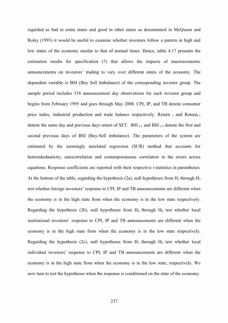
237
regarded as bad in some states and good in other states as documented in McQueen and
Roley (1993) it would be useful to examine whether investors follow a pattern in high and
low states of the economy similar to that of normal times. Hence, table 4.17 presents the
estimation results for specification (7) that allows the impacts of macroeconomic
announcements on investors’ trading to vary over different states of the economy. The
dependent variable is BSI (Buy Sell Imbalance) of the corresponding investor group. The
sample period includes 318 announcement day observations for each investor group and
begins from February 1995 and goes through May 2008. CPI, IP, and TB denote consumer
price index, industrial production and trade balance respectively. Return t and Returnt-1
denote the same day and previous days return of SET. BSI t-1 and BSI t-2 denote the first and
second previous days of BSI (Buy-Sell imbalance). The parameters of the system are
estimated by the seemingly unrelated regression (SUR) method that accounts for
heteroskedasticity, autocorrelation and contemporaneous correlation in the errors across
equations. Response coefficients are reported with their respective t-statistics in parentheses.
At the bottom of the table, regarding the hypothesis (2a), null hypotheses from H1 through H3
test whether foreign investors’ response to CPI, IP and TB announcements are different when
the economy is in the high state from when the economy is in the low state respectively.
Regarding the hypothesis (2b), null hypotheses from H4 through H6 test whether local
institutional investors’ response to CPI, IP and TB announcements are different when the
economy is in the high state from when the economy is in the low state respectively.
Regarding the hypothesis (2c), null hypotheses from H7 through H9 test whether local
individual investors’ response to CPI, IP and TB announcements are different when the
economy is in the high state from when the economy is in the low state, respectively. We
now turn to test the hypotheses when the response is conditioned on the state of the economy.

238
In the high state of the economy, we find significant relationship between the
response of foreign investors and the surprise component of the industrial production
announcements. Similar to the result obtained for the whole period, foreigners are found to
sell/buy stocks following a positive/negative surprise about the economy which shows that
they act in a contrarian manner around industrial production announcements which is also not
in line with the stated hypothesis since they are expected to behave in a momentum style
around macroeconomic announcements. In terms of CPI and TB announcements, we find no
significant response for foreigners to these announcements in the high state of the economy.
For local institutional investors, we come up with different findings in the high state
compared to low or medium state of the economy. For example, unlike the low or medium
state of the economy, we find significant reaction to both inflation and IP announcements in
the high state. In terms of inflation announcements, they tend to sell/buy stocks in response to
an increase/decrease in the inflation index which shows that they tend to follow the contrarian
trading strategy with respect to inflation announcements, inconsistent with the prediction of
hypothesis (1b). In terms of IP announcements, we find a positive significant response to IP
announcements in the high state of the economy. They are found to buy/sell stocks after
positive/negative surprises in IP announcements showing that they act in a momentum
manner around IP announcements in the high state of the economy. This behaviour is in line
with the prediction in hypothesis (1b). Similar to the whole period, local institutions are also
found to give significant reactions to TB announcements in the high state of the economy.
They tend to buy/(sell) stocks at good/(bad) surprises in TB announcements indicating that
they behave in a momentum style around TB announcements which is consistent with the
prediction in hypothesis (1b). For local individual investors, we find no statistically
significant reaction to any of the announcement in the high state of the economy.

239
When turning to the low growth period, we find no statistically significant response
for foreigners to any type of announcement. For local institutions, similar to the whole
period, we document statistically significant reaction around TB announcements. We find
that they sell/buy stocks following positive/negative surprises in the trade balance
announcements showing that they pursue contrarian trading around TB announcements,
which is not in line with the prediction in hypothesis (1b). For local individuals, we document
significant negative response to the surprises in inflation announcements. They tend to
sell/buy stocks in response to positive surprises about the inflation. This behaviour shows that
they pursue contrarian trading style which is consistent with the expectation in hypothesis
(1c).
In the medium growth economy, in terms of foreigners, the only significant reaction is
found for the inflation announcement, using the baseline specification (6), though less
significant. Foreigners are found to buy/sell stocks after positive/negative inflation news
showing that they behave in a momentum trading style consistent with the prediction in
hypothesis (1a). Similar to foreigners, local individuals are only found to give significant
reaction to the surprise component of the inflation news. They tend to sell/buy stocks
following good/bad news about inflation which shows that they engage in negative feedback
strategy which is also consistent with the prediction in hypothesis (1c). Apart from inflation
announcements, we find no significant response for local individuals to IP and TB
announcements in the medium state of the economy. Unlike foreigners and local individuals,
we find no significant evidence of response for local institutions to any type of announcement
in the medium state of the economy.

240
When moving to test the sub hypotheses from H1 through H9 that whether the state
dependent coefficients of each investor type for each economic announcement are
statistically the same, we cannot reject seven out of nine hypotheses. The only hypothesis
which is rejected at the 10% significance level is that the responses of institutional investors
to trade balance surprises are the same across high and low states of the economy (H6). A
possible explanation for insignificant results of sub hypotheses can be resulted from having
same level of uncertainty in the high and low state of the economy. Since the economy
includes higher uncertainty in the high and low states relative to normal states investors may
not receive precise signals during these periods as they receive in normal periods. Receiving
more mixed signals in these two states of the economy can hinder investors from acting
precisely as they behave in the same manner around macroeconomic announcements.
Finally, similar to the results obtained from specification (6), a point worth
mentioning here is that all our control variables are also found to be highly significant in
response of all types of investors.

241
Table 4.17 Responses of different types of investors to macroeconomic announcementsduring high and low states of the economy
Foreigners institutions individualsintercept 0.018 -0.01 -0.005
(2.69)*** (-0.85) (-1.44)BSI t-1 0.298 0.404 0.265
(6.65)*** (10.33)*** (5.73)***BSI t-2 0.144 0.135 0.196
(2.94)*** (2.28)** (3.39)***Return t 1.73 Na -1.22
(3.93)*** Na (-5.18)***Return t-1 1.68 1.683 -1.15
(2.37)*** (1.78)* (-3.73)***
Announcementshigh growth (boom)Consumer Price Index (CPI) 0.013 0.127 0.008
(0.15) (1.67)* (0.12)Industrial Production (IP) -0.053 0.03 0.01
(-3.31)*** (1.89)* (0.9)Trade Balance (TB) 0.08 0.577 -0.21
(0.42) (2.67)*** (-1.63)Low growth (recession)Consumer Price Index (CPI) -0.014 0.03 0.035
(-0.41) (0.48) (1.91)*Industrial Production (IP) -0.018 -0.024 0.015
(-1.09) (-0.94) (1.35)Trade Balance (TB) 0.001 -0.009 0.001
(0.84) (-4.05)*** (0.85)Medium GrowthConsumer Price Index (CPI) -0.068 0.023 0.068
(-2.05)** (0.27) (2.1)**Industrial Production (IP) -0.003 -0.025 0.006
(-0.31) (-1.35) (1.01)Trade Balance (TB) -0.015 -0.035 0.016
(-0.84) (-1.1) (1.39)----------------------------------------------------------------------------------------------------------------Foreigners Local Institutions Local Individualschi-square Prob chi-square Prob chi-square Prob
H1: bH=bL for CPI 0.09 0.76 H4: bH=bL for CPI 0.92 0.34 H7: bH=bL for CPI 0.15 0.70
H2: bH=bL for IP 2.17 0.14 H5: bH=bL for IP 2.81 0.10 H8: bH=bL for IP 0.12 0.73
H3: bH=bL for TB 0.17 0.67 H6: bH=bL for TB 7.43 0.00*** H9: bH=bL for TB 2.67 0.10
Table 4.13 shows the estimation results for specification (7) estimated by seemingly unrelated regressionmethod that allows for heteroskedasticity, autocorrelation and contemporaneous correlation in the residuals. The

242
sample period includes 318 announcement day observations for each investor categories from February 1995 toMay 2008. Total system (balanced) observations are 954. Regression coefficients are reported with theirrespective t statistics in parentheses. The dependent variable is the BSI (Buy-Sell Imbalance = ( )( )) ofthe corresponding investor group. BSIt-1 and BSIt-2 denote the first and second lag of BSI respectively. Returntand Returnt-1 denote the same day and previous day’s return of the SET respectively. *, **, and *** indicatesignificance at the 10, 5 and 1 percent levels, respectively. At the bottom of the table, null hypotheses from H1through H3 test whether foreign investors’ responses to CPI, IP and TB announcements in the high state aredifferent from the responses to CPI, IP, and TB announcements in the low state respectively. Null hypothesesfrom H4 through H6 test whether local institutions’ responses to CPI, IP and TB announcements in the high stateare different from the responses to CPI, IP, and TB announcements in the low state respectively. Nullhypotheses from H7 through H9 test whether local individuals’ responses to CPI, IP and TB announcements inthe high state are different from the responses to CPI, IP, and TB announcements in the low state respectively.Na is used for contemporaneous return in the local institutions regression due to having no correlation betweenlocal returns and the reaction of local institutions around macroeconomic announcements.
4.6.3 Responses to macroeconomic announcements conditional on the state of themarket
As mentioned in section 4.2.3, recent underlying market conditions (bull/bear
markets) were found to have different influences on stock returns. For example, Klein and
Rosenfeld (1987) document divergent results for the identical events during bull and bear
markets. In this context, it would be useful to examine whether investors exhibit the same
type trading behaviours around macroeconomic announcements over different conditions of
the stock market. Hence, table 4.18 shows the estimation results for specification (8) that
allows the effects of macroeconomic announcements on investor sentiment to vary over
different states of the market. The dependent variable is the BSI (Buy Sell Imbalance) of the
corresponding investor group. The sample period includes 318 announcement day
observations for each investor group and begins from February 1995 and goes through May
2008. CPI, IP, and TB denote consumer price index, industrial production and trade balance
respectively. Return t and Returnt-1 denote the same day and previous days return of SET
respectively. BSI t-1 and BSI t-2 denote the first and second previous days of BSI (Buy-Sell
imbalance) respectively. The parameters of the system are estimated by the non-linear
iterated seemingly unrelated regression (SUR) method that accounts for heteroskedasticity,

243
autocorrelation and contemporaneous correlation in the errors across equations. The response
coefficients are reported with their respective t-statistics in parentheses. At the bottom of the
table, null hypotheses from H10 through H12, regarding the hypothesis (3a), test whether
foreign investors’ responses to CPI, IP and TB announcements in the bull market periods are
different from the responses to CPI, IP, and TB announcements in the bear market periods
respectively. Null hypotheses from H13 through H15, regarding the hypothesis (3b), test
whether local institutions’ responses to CPI, IP and TB announcements in the bull market
periods are different from the responses to CPI, IP, and TB announcements in the bear market
periods respectively. Null hypotheses from H16 through H18, regarding the hypothesis (3c),
test whether local individuals’ responses to CPI, IP and TB announcements in the bull market
periods are different from the responses to CPI, IP, and TB announcements in the bear market
periods respectively.
We now turn to test our hypotheses after conditioning the response on the state of the
stock market. In the bull market periods, we find no significant response for any type of
investors to any announcement which is not consistent with the predictions, because investors
are expected to exhibit more momentum or contrarian behaviour around macroeconomic
announcements during bull market periods.
For the bear market periods we come up with significant findings for each investor
group. For example, of foreign investors, we document significant reaction to inflation
announcements. They tend to buy/sell stocks following good/bad news about the inflation
which indicates that they act in a momentum manner with respect to inflation
announcements, consistent with the prediction in hypothesis (1a). For local institutions, we
document significant response around trade balance announcements. They tend to sell/buy

244
stocks following good/bad news about the economy which indicates that they pursue
contrarian trading strategy around TB announcements in the bear market period which is not
in line with the prediction in hypothesis (1b). When turning to local individuals, we find
significant response around both inflation and trade balance announcements. They are found
to sell/buy stocks in response to good/bad news about inflation which suggests that they
pursue a contrarian trading strategy around inflation announcements, consistent with what is
predicted by hypothesis (1c). In a similar vein, we find strong evidence of a significant
relationship between reaction of local individuals and the surprise component of the trade
balance announcement, but in an opposite direction. They are found to buy/sell stocks at
good/bad trade balance news which suggests that they engage in a momentum trading
strategy which is not in line with the prediction in hypothesis (1c).
When moving to the analysis of normal market periods we come up with interesting
findings for foreigners and local individuals, because in our baseline specification (6) both
investors are found to give some significant responses to some type of macroeconomic
announcements. However, here, in terms of both investors we find no significant reaction to
any type of announcement. Unlike the findings for foreigners and local individuals, our
findings for local institutions are similar with what is found in our baseline specification (6).
In other words, they tend to sell/buy stocks on good/bad TB news showing that they follow
contrarian trading strategy with respect to TB announcements which is also not consistent
with the prediction in hypothesis (1b).
For testing the sub hypotheses, regarding the hypotheses (3a), 3(b), and (3c), from H10
through H18 that whether the market state dependent coefficients of each investor type for
each economic announcement are statistically same we find that three out of nine hypotheses

245
can be statistically rejected. The first two hypotheses are rejected for local institutions. First,
we find that the hypothesis that the responses of local institutions to CPI announcements in
the bull and bear market periods are the same (H13) can be rejected at the 0.05 significance
level. Second, the hypothesis that the responses of local institutions to TB announcements in
the bull and bear market periods are same (H15) can be rejected at the 0.01 significance level.
The third hypothesis is rejected for local individuals. Similar to the finding for local
institutions, we find that the hypothesis that the responses of local individuals to CPI
announcements in the bull and bear market periods are same (H13) can be rejected at the 0.05
significance level.
Finally, in a similar vein, it is also noteworthy that our control variables are found to
be highly significant explanatory variables as are found in specification (6) and specification
(7) for each equation in the system.

246
Table 4.18 Responses of different types of investors to macroeconomic announcementsduring bull and bear states of the economy.
Foreigners Institutions Individualsintercept 0.018 -0.017 -0.003
(2.64)*** (-1.46) (-0.93)BSI t-1 0.297 0.405 0.271
(6.65)*** (10.41)*** (5.92)***BSI t-2 0.137 0.131 0.195
(2.71)*** (2.27)** (3.28)***Return t 1.716 na -1.14
(2.39)** (-3.74)***Return t-1 1.815 1.663 -1.28
(4.05)*** (1.72)* (-5.67)***
Announcementsbull market periodsConsumer Price Index (CPI) -0.007 0.143 0.01
(-0.13) (1.55) (0.36)Industrial Production (IP) -0.005 0.001 0.001
(-0.49) (0.08) (0.15)Trade Balance (TB) -0.02 0.017 0.007
(-0.56) (0.22) (0.29)bear market periodsConsumer Price Index (CPI) -0.069 -0.087 0.095
(-3.85)*** (-1.24) (4.47)***Industrial Production (IP) -0.063 0.079 -0.006
(-1.28) (1.32) (-0.18)Trade Balance (TB) -0.062 -0.512 0.172
(-0.47) (-5.06)*** (1.72)*normal market periodsConsumer Price Index (CPI) -0.01 0.149 0.007
(-0.25) (1.45) (0.23)Industrial Production (IP) -0.02 -0.015 0.013
(-1.73) (-0.92) (1.61)Trade Balance (TB) 0.001 -0.008 0.008
(0.28) (-2.08)** (0.63)
Foreigners Local Institutions Local Individualschi-square Prob chi-square Prob chi-square Prob
H10: bBE=bBU for CPI 1.14 0.28 H13:bBE=bBUfor CPI 3.87 0.04** H16: bBE=bBU for CPI 5.62 0.02**
H11: bBE=bBU for IP 1.36 0.24 H14: bBE=bBU for IP 1.45 0.22 H17: bBE=bBU for IP 0.04 0.83
H12: bBE=bBU for TB 0.06 0.80 H15: bBE=bBU for TB 17.18 0.0*** H18: bBE=bBU for TB 2.55 0.11
Table 4.14 shows the estimation results for specification (8) estimated by seemingly unrelated regressionmethod that allows for heteroskedasticity, autocorrelation and contemporaneous correlation in the residuals. Thesample period includes 318 announcement day observations for each investor categories from February 1995 toMay 2008. Total system (balanced) observations are 954. Regression coefficients are reported with their

247
respective t statistics in parentheses. The dependent variable is the BSI (Buy-Sell Imbalance = ( )( ) ) ofthe corresponding investor group. BSIt-1 and BSIt-2 denote the first and second lag of BSI. Returnt and Returnt-1denote the same day and previous day’s return of SET respectively. *, **, and *** indicate significance at the10, 5 and 1 percent levels, respectively. At the bottom of the table, null hypotheses from H10 through H13 testwhether foreign investors’ responses to CPI, IP and TB announcements in the bear state are different from theresponses to CPI, IP, and TB announcements in the bull state respectively. Null hypotheses from H14 throughH16 test whether local institutions’ responses to CPI, IP and TB announcements in the bear state are differentfrom the responses to CPI, IP, and TB announcements in the bull state respectively. Null hypotheses from H17through H19 test whether local individuals’ responses to CPI, IP and TB announcements in the bear state aredifferent from the responses to CPI, IP, and TB announcements in the bull state respectively. Na is used forcontemporaneous return in the local institutions regression due to having no correlation between local returnsand the reaction of local institutions around macroeconomic announcements.
4.6.4 Responses to economic announcements across sub-periods
There was a pervasive financial crisis in Pacific-Asia region during our observation
period, which started in Thailand on 2 July 1997. As mentioned previously, if investors lose
money by engaging in a specific strategy their trading patterns are not expected to continue
persistently, since investors are expected to learn from their trading experiences. In this
context, the Asia crisis could have altered fundamental trading behaviour of investors which
can lead to different responses across pre- and post-crisis periods. Therefore regarding the
hypotheses (4a), (4b), and (4c), we now test whether investors continue to exhibit same
trading behaviours around macroeconomic announcements in the post-crisis period as were
found in the pre-crisis period.
Table 4.19 shows estimation results under specification (9) that allows the effects of
macroeconomic announcements on investor sentiment to vary over different sub-periods of
the crisis to see whether our inferences change through our observation period. The
dependent variable is the BSI (Buy Sell Imbalance) of the corresponding investor group. The
sample period includes 318 announcement day observations for each investor group and
begins from February 1995 and goes through May 2008. CPI, IP, and TB denote consumer

248
price index, industrial production and trade balance respectively. Return t and Returnt-1
denote the same day and previous days return of SET respectively. BSI t-1 and BSI t-2 denote
the first and second previous days of BSI (Buy-Sell imbalance), respectively. The parameters
of the system are estimated by the seemingly unrelated regression (SUR) method that
accounts for heteroskedasticity, autocorrelation and contemporaneous correlation in the errors
across equations. Response coefficients are reported with their respective t-statistics in
parentheses. At the bottom of the table, null hypotheses from H19 through H21, regarding the
hypothesis 4a, test whether foreign investors’ responses to CPI, IP and TB announcements in
the pre-crisis periods are different from the responses to CPI, IP, and TB announcements in
the post-crisis periods respectively. Null hypotheses from H22 through H24, regarding the
hypothesis 4b, test whether local institutions’ responses to CPI, IP and TB announcements in
the pre-crisis periods are different from the responses to CPI, IP, and TB announcements in
the post-crisis periods respectively. Null hypotheses from H25 through H27, regarding the
hypothesis 4c, test whether local individuals’ responses to CPI, IP and TB announcements in
the pre-crisis periods are different from the responses to CPI, IP, and TB announcements in
the post-crisis periods respectively. We now move to test the hypotheses mentioned in section
4.2. 3.
In the pre-crisis period, unlike the whole period, we find no significant response for
any type of investor around inflation announcements. However, all players are found to give
significant response around IP and TB announcements. For example, foreigners are found to
sell/buy on good/bad IP news while both local institutions and local individuals are found to
have opposite reaction to the same IP news in the pre-crisis period. This finding suggests that
while foreigners tend to pursue a contrarian trading strategy local institutions and local

249
individuals are found to follow a momentum trading strategy around inflation
announcements.
However, when we look at the post-crisis period we find no significant response from
foreigners and local individuals to any type of announcement. It is rather interesting since it is
the longest period including 72 % of the all observations. However, for local institutions,
similar to the findings in baseline specification (6), we find significant response around trade
balance announcements. They tend to sell/buy stocks after good/bad trade balance news
which shows that they behave in a contrarian manner with respect to TB announcements in
the post-crisis period which is not consistent with the stated hypothesis in (1b).
Finally, we move to the crisis period and find that inflation surprises have significant
effect on the trading behaviour of foreign investors. They are found to buy/sell stocks on
good/bad inflation news which suggests that they tend to follow momentum trading strategy
which is consistent with the prediction in hypothesis (1a). In terms of IP and TB
announcements they are not found to have significant affect on the sentiment of foreign
investors. Similar to foreign investors, we also find significant response of local individuals
to inflation announcements as well. They tend to sell on good inflation news and buy on bad
inflation news which shows that they behave in a contrarian manner, and is in line with the
stated hypothesis in (1c). Furthermore, local individuals are also found to react significantly
to TB announcements in the crisis period. They buy/sell stocks on good/bad trade balance
news showing an evidence of momentum trading strategy which is not consistent with the
predictions. As a last, similar to local individuals, we also find significant evidence of
response of local institutions to TB announcements, but with opposite sign in the crisis
period. They tend to sell/buy stocks after good/bad TB news which shows that they act in a

250
contrarian manner with respect to TB announcements which is not in line with what is
predicted in hypothesis (1b).
Finally, when we turn to test the sub hypotheses, regarding the hypothesis (4a), (4b),
and (4c), from H19 through H27 we come up with interesting findings especially in terms of IP
and TB announcements. We find that all three types of investors change their behaviours
around IP and TB announcements in the post-crisis period compared to pre-crisis period.
However, in terms of inflation announcements their responses are not found to change across
the pre- and post-crisis periods.
Finally, it is also worth noting that all our control variables are found highly
significant in each equation in the system as under previous specifications. Therefore, it is not
likely to obtain unbiased estimates of the impact of the macroeconomic news in the absence
of our control variables.

251
Table 4.19 Responses of different types of investors to macroeconomic announcementsacross sub-periods
Foreigners Institutions Individualsintercept 0.014 -0.011 -0.003
(2.2)** (-0.91) (-0.92)BS t-1 0.295 0.41 0.262
(6.91)*** (11.02)*** (5.8)***BS t-2 0.135 0.137 0.187
(2.81)*** (2.34)** (3.26)***Return t 1.69 Na -1.12
(2.4)** (-3.56)***Return t-1 1.71 1.49 -1.212
(3.18)*** (1.66)* (-4.54)***
Announcementspre-crisis periodsConsumer Price Index (CPI) -0.182 0.127 0.114
(-0.9) (0.54) (0.72)Industrial Production (IP) -0.06 0.025 0.015
(-4.69)*** (1.81)* (2.49)**Trade Balance (TB) 0.301 0.74 -0.415
(1.69)* (2.62)*** (-4.62)***
post-crisis periodsConsumer Price Index (CPI) 0.02 0.026 0.008
(0.52) (0.36) (0.4)Industrial Production (IP) -0.003 -0.012 0.002
(-0.36) (-0.93) (0.57)Trade Balance (TB) 0.001 -0.007 0.001
(0.19) (-2.12)** (0.72)crisis periodsConsumer Price Index (CPI) -0.073 0.036 0.07
(-2.54)** (0.47) (2.65)***Industrial Production (IP) -0.01 -0.022 0.018
(-0.72) (-0.56) (0.94)Trade Balance (TB) -0.13 -0.592 0.161
(-1.41) (-4.73)*** (2.34)**
Foreigners Local Institutions Local Individualschi-square Prob chi-square Prob chi-square Prob
H19: bPRE=bPOST for CPI 0.98 0.32 H22: bPRE=bPOST for CPI 0.17 0.67 H25:bPRE=bPOST for CPI 0.44 0.50
H20:bPRE=bPOST for IP 13.66 0.00*** H23: bPRE=bPOST for IP 3.3 0.06* H26: bPRE=bPOST for IP 2.82 0.09*
H21:bPRE=bPOST for TB 2.85 0.09* H24:bPRE=bPOST for TB 7.01 0.00*** H27:bPRE=bPOST for TB 21.42 0.00***

252
Table 4.15 shows the estimation results for specification (9) estimated by seemingly unrelated regressionmethod that allows for heteroskedasticity, autocorrelation and contemporaneous correlation. The sample periodincludes 318 announcement day observations for each investor categories from February 1995 to May 2008.Total system (balanced) observations are 954. Regression coefficients are reported with their respective tstatistics in parentheses. The dependent variable is the BSI (Buy-Sell Imbalance = ( )( ) ) of thecorresponding investor group. BSIt-1 and BSIt-2 denote the first and second lags of BSI respectively. Returnt andreturnt-1 denote the same day and previous day’s return in SET respectively. *, **, and *** indicate significanceat the 10, 5 and 1 percent levels, respectively. At the bottom of the table, null hypotheses from H19 through H21test whether foreign investors’ responses to CPI, IP and TB announcements in the pre-crisis period are differentfrom the responses to CPI, IP, and TB announcements in the post-crisis period respectively. Null hypothesesfrom H22 through H24 test whether local institutions’ responses to CPI, IP and TB announcements in the pre-crisis period are different from the responses to CPI, IP, and TB announcements in the post-crisis periodrespectively. Null hypotheses from H25 through H27 test whether local individuals’ responses to CPI, IP and TBannouncements in the pre-crisis period are different from the responses to CPI, IP, and TB announcements in thepost-crisis period respectively.
4.6.5 Responses variation of investors to same economic announcements
As a complementary, we now move to analyse whether the responses of investors are
different from each other around same macroeconomic announcements, because in order to
evaluate the issue from a comparative viewpoint, investors’ behaviours should be examined
simultaneously in the system rather than looking at their individual coefficients. Table 4.20
summarizes the results of the hypotheses that test whether there are statistically response
distinctions among different types of investors to same macroeconomic announcements.
Panel A shows the results that the responses of foreigners and local institutions to
corresponding macroeconomic announcement are same. CPI, IP, TB denote consumer price
index, industrial production and trade balance respectively. This study has investigated the
investor sentiment around macroeconomic announcements with four different specifications.
The first one is the base line specification including the whole sample and other ones are the
state-dependent specifications each of which includes three subsamples. Therefore, investor
sentiment around macroeconomic announcements has been examined from ten different
perspectives. Accordingly, in each panel in table 4.16, the left column represents these
perspectives. The rest three columns show the results for the corresponding announcements

253
namely CPI, IP and TB. For example, in panel A, the hypothesis that the responses of
foreigners and local institutions to industrial production announcements are same in the
whole period is rejected with a p-value of 0.03. Other results are interpreted similarly. Panels
B and C show the results of the tests for foreigners and local individuals and for local
institutions and local individuals, respectively, in the same manner. In order to test these
kinds of hypotheses we have to put restrictions on coefficients across equations since there
are three separate equations for each of the investor’s type. The parameters of the system are
estimated by seemingly unrelated regression (SUR) method that accounts for
heteroskedasticity, autocorrelation and contemporaneous correlation in the errors across
equations.
Having described the table 4.20, we now turn to interpret the results. As previously
mentioned in all specifications, foreigners and local institutions are found to pursue
momentum trading strategies, whereas local individuals pursue contrarian trading strategy
with respect to past returns. In this set up, having followed Vieru, Perttunen, and Schadewitz,
(2006), we translate momentum (contrarian) behaviour into a tendency to buy (sell) stocks on
good news and sell (buy) stocks on bad news. Given the above, accordingly, foreigners and
local institutions are expected to behave in the same manner, whereas the local individual’s
behaviour is expected to differ from them around macroeconomic announcements for all
specifications.
When turning to the panel A, in nine out of thirty cases, we find statistical response
distinction between foreigners and local institutions. In other words, for twenty one of the
thirty cases in panel A, our results are consistent with the prediction. Statistical response
distinctions are found for industrial production announcement observed in the high state of

254
the economy and the pre-crisis period. For trade balance announcement the response
distinction is observed in the whole period, high and low states of the economy, bear and
normal market periods and in the post- and crisis periods.
In the panel B, we find that the responses of foreigners and local individuals are
statistically different from each other in ten out of thirty cases. Or, put differently, in ten out
of thirty cases our results are in line with what is predicted. In four out of these ten cases a
response distinction is found for CPI news which is observed in the whole period, medium
growth, bear market period, and crisis period. In the second four out of ten cases we find that
the responses of foreigners and local individuals are different from each other for IP
announcements observed in the whole period, high growth, normal market period and pre-
crisis period, and in the last two out of these ten cases, a response distinction is also found for
TB news observed in the pre-crisis and crisis period.
Finally, in panel C, for nine out of thirty cases we find significant response
distinctions between local institutions and local individuals. That is to say, for nine out of
thirty cases our findings are consistent with the predictions. The first response difference is
found for inflation announcements which is observed in the bear market period, and the other
eight response differences are found for TB announcements observed in the whole period,
high growth period, low growth period, bear market period, normal market period, pre-crisis
period, post-crisis and the crisis period.

255
Table 4.20 Summary statistics of the response distinctions among investors aroundmacroeconomic announcements
Panel A Foreigners vs InstitutionsCPI IP TB
Whole period (6) 0.17 0.42 0.03**High growth (boom)(7) 0.21 0.00*** 0.09*Low growth (recesssion)(7) 0.55 0.88 0.00***Medium growth (7) 0.30 0.29 0.59Bull market period(8) 0.22 0.77 0.67Bear market period(8) 0.81 0.11 0.00***Normal market period(8) 0.18 0.67 0.05**Pre-crisis period(9) 0.22 0.00*** 0.31Post-crisis period(9) 0.94 0.60 0.06*Crisis period(9) 0.17 0.17 0.00***
Panel B Foreigners vs IndividualsCPI IP TB
Whole period (6) 0.03** 0.06* 0.63High growth (boom)(7) 0.97 0.01 0.34Low growth (recesssion)(7) 0.32 0.19 0.92Medium growth (7) 0.02** 0.54 0.27Bull market period(8) 0.82 0.69 0.62Bear market period(8) 0.00*** 0.46 0.30Normal market period(8) 0.79 0.07 0.91Pre-crisis period(9) 0.38 0.00*** 0.00***Post-crisis period(9) 0.82 0.65 0.83Crisis period(9) 0.00*** 0.38 0.06*
Panel C Institutions vs IndividualsCPI IP TB
Whole period (6) 0.80 0.27 0.05**High growth (boom)(7) 0.33 0.39 0.00***Low growth (recesssion)(7) 0.96 0.19 0.00***Medium growth (7) 0.66 0.15 0.18Bull market period(8) 0.17 0.97 0.89Bear market period(8) 0.03** 0.26 0.00***Normal market period(8) 0.24 0.16 0.05**Pre-crisis period(9) 0.97 0.54 0.00***Post-crisis period(9) 0.83 0.31 0.04**Crisis period(9) 0.68 0.82 0.00***
Table 4.16 provides the p-values of the hypotheses for the response distinctions among investors of thecorresponding macroeconomic announcement. CPI, IP, TB denote consumer price index, industrial productionand trade balance respectively. Panel A shows the results of the hypotheses that the responses of foreigners andlocal institutions to corresponding macroeconomic announcement are same. Panel B shows the results of thehypotheses that the responses of foreigners and local individuals to corresponding macroeconomicannouncement are same. Panel C shows the results of the hypotheses that the responses of local institutions and
256
local individuals to corresponding macroeconomic announcement are same. The number in brackets representsthe specifications as mentioned in methodology section. *, **, and *** indicate significance at the 10, 5 and 1percent levels, respectively.
4.7 Discussion
One may argue that using dummy variables rather than market expectations would be
more appropriate in analyzing the trading behaviour of market participants. However, it
seems that using dummy variables in this kind of analysis has more disadvantages if there are
more than one announcement releases at the same time. For example, in our case, the trade
balance and industrial production data are released at the same time by the Bank of Thailand.
Therefore, it would be impossible to separate the effects of those announcements if we used
dummy variables in place of the surprise parts of these macroeconomic announcements.
Additionally, according to the market efficiency hypothesis, only new and unpredictable
component of information is expected to move asset prices. The role of “new information” in
the test of market efficiency and in the formation of asset prices has strong intuitive appeal.
However, to explore this some references have to be created to capture the unexpected
component of the news. By its very nature, market participants are not always have the same
forecast for a particular variable and all surveys are made with only very few members of
market participants. We have no way of knowing which market participants have lower,
higher or exactly the same forecast compared to the market expected value for that particular
variable before the release of that announcement.
It is worth noting that the median of analysts’ expectations for a particular variable is
mostly known in advance by the market participants. Because, market professionals are
usually demanded to speak to media about market expectations regarding particular
forthcoming macroeconomic announcement. These market professionals are also subscribers

257
of economic survey organizations that produce these market expectations. Therefore, this
median of analysts’ expectations is generally released to the public before the release of
particular announcement. From that point onwards, this median of analysts’ expectation value
becomes market expected value de facto accepted by the market participants. Hence, after the
announcement is made the question then is whether market participants have the same
knowledge or beliefs about how such “new information” (the difference between the actual
data and the median of analysts’ expectations) will affect the opportunity set available. The
more the market participants have divergent beliefs about the implications of the new
information the more will be the increase in trading volume, because market participants try
to understand each others’ beliefs while forming their own beliefs. Trading volume jumps as
different market participants rebalance their portfolios in response to their own beliefs and
their perception of others about the implication of the new information on asset prices which
then leads to changes in the levels to re-establish equilibrium pricing (Keem and Sheen,
2000).
In the light of the above discussion, there is a strong case for taking the median of
analysts’ expectations as a reference point, rather than using dummy variables. Thus, our
study is the first to suggest and employ the median of analysts’ expectations as an
explanatory variable in the regression, while explaining the behaviour of different types of
investors around news releases.
4.8 Conclusion
This study has investigated the reactions of different types of investors to
macroeconomic announcements in the stock exchange of Thailand. Previous studies (e.g.,

258
Grinblat and Keloharju, 2000, Kim and Wei, 2002, Dahlquist and Robertson, 2004, Griffin,
Nardari, and Stulz, 2004, and Richard 2005) documented a number of empirical evidences
showing that foreign and local institutional investors act as momentum traders, whereas
individual investors act in a contrarian manner with respect to past returns. In this study,
following Vieru, Perttunen, and Schadewitz (2006), momentum (contrarian) behaviour is
translated into a tendency to buy (sell) stocks following good news and sell (buy) following
bad news around macroeconomic announcements. Based on this finding, we analyze whether
the responses of investors to economic announcements are in line with their stylized facts
documented with respect to past returns.
This study begins with analyzing investor’s reaction for the whole period as a base
line specification. We find that, on average, foreign investors buy stocks on good inflation
news and sell stocks on bad inflation news, which is consistent with the momentum
investment style. However, the same foreigners are found to behave in a different style
around IP announcements. We document that they tend to buy/sell on bad/good IP news,
indicating that they act in a contrarian manner around IP announcements which is not in line
with the prediction. In terms of local individuals, we document opposite behaviour compared
to foreigners around inflation announcements. We find that they sell/(buy) stocks after
good/(bad) inflation news suggesting evidence of negative feedback trading which is
consistent with what is predicted. Unlike foreigners and local individuals, when turning to the
reaction of local institutions we find no significant responses of them to inflation and IP
announcements, but trade balance. They are found to sell/(buy) stocks in response to
positive/(negative) news about trade balance which shows that they engage in a negative
feedback trading strategy around TB announcements.

259
However, when the investor response is conditioned on different states of the
economy, in contrast to the findings for the whole period, local institutions are now found to
give positive response to TB announcements in the high state of the economy. This indicates
that they act in a momentum manner with respect to TB news in the high state of the
economy which is consistent with the predictions. Besides TB news we also find significant
response for local institutions to both inflation and industrial production announcements in
the high state of the economy. They tend to buy/(sell) stocks on good/bad IP news which
shows that they pursue momentum trading strategy around IP announcements which is
consistent with the predictions. With respect to inflation announcements, local institutions are
found to behave oppositely compared to other two announcements. We find that they
sell/(buy) stocks following good/bad news about the inflation. When turning to foreign
investors, we find that they react significantly to only IP news in the high state of the
economy. They tend to sell/buy stocks on bad/(good) news about the economy indicating that
they behave in a contrarian investment style which is not consistent with what is predicted for
them. This finding is also similar to the finding found for the whole period. Unlike both
investors, we find no significant response of local individuals to any type of announcement in
the high state of the economy.
In the recession period, we come up with interesting findings for local institutions, as
they react completely opposite to IP and TB announcements compared to high state of the
economy. They tend to sell/(buy) stocks on good/bad news about IP and TB which shows that
they engage in a momentum investment style around these two announcements. It is worth
noting that dividing the whole period into sub-periods as high/low/medium is important,
because sometimes reactions of investors in one period can be concealed by their behaviours
in other periods, as is for local institutions in our case, by means of lowering the average

260
significance level. In terms of local individuals, we only find significant reaction to inflation
announcements as found for the whole period and in the boom period. They sell/(buy) stocks
following good/bad news about inflation showing that they act in a contrarian manner which
is in line with the predictions. For foreigners, we find no significant response to any type of
announcement in the recession period.
When we condition the responses of investors over different states of the stock
market, in contrast to the findings for the whole period, we find no significant reaction for
any type of investors to any announcement in the bull market periods which is in contrast to
the prediction since investors are expected to exhibit more momentum or contrarian
behaviour around macroeconomic announcements during the bull market period.
In the bear market period, local individuals give significant responses to inflation and
trade balance announcements. We find that they tend to sell/buy stocks following good/bad
inflation news in the bear market period, which shows that they engage in a contrarian trading
strategy, consistent with what is predicted. Local individuals also buy/(sell) stocks after
positive/negative TB news indicating that they act in a momentum manner with respect to TB
announcements which is not in line with the prediction. In the bear market period, unlike the
results for the whole period, foreigners are found to give significant response to only inflation
announcements. Similar to the findings found for the whole period they also pursue a
momentum trading strategy around inflation announcements. In a similar vein, local
institutions are also found to give significant reactions to TB announcements as is found for
the whole period. They tend to sell/(buy) stocks on good/(bad) TB news indicating that they
act in a contrarian manner which is not in line with the predictions in hypothesis (1b).

261
When the investor response is made conditional on crisis sub-periods to see whether
their behaviours have changed through time, we come up with some interesting results. For
example, unlike the results for the whole period, for local individuals we find significant
responses to IP and TB announcements in the pre-crisis period. They tend to buy/(sell) stocks
on bad/(good) IP news which shows that they behave as momentum traders around IP
announcements as predicted in the pre-crisis period, whereas they act in an opposite manner
around TB announcements indicating an evidence of contrarian trading which is not in line
with the prediction. For foreigners and local institutions, we find that both groups of investors
give significant reactions to IP and TB announcements in the pre-crisis period. On the IP
announcement days, foreigners sell/buy stocks on good IP news while local institutions react
oppositely. On the TB announcement days, both are found to react similarly i.e. they both
buy/sell stocks on good/bad TB news indicating that both pursue a momentum trading
investment style around TB announcements.
In the post-crisis period, the results are quite interesting. We find no significant
responses of foreigners and local individuals to any type of announcement. However, it is
here useful to mention that this period is the longest period which includes 72 % of all
observations. The only significant reaction is found for local institutions in this period, which
is similar to the findings for the whole period. That is, local institutions tend to sell/(buy)
stocks on good/(bad) TB news, suggesting that they engage in contrarian investment trading
in the post-crisis period, which is not consistent with what is expected for local institutions.
In the crisis period, the results for all players are completely similar to the findings for
the bear market period. That is, foreigners tend to buy/(sell) stocks on good/(bad) inflation
news showing adaptation of a momentum trading strategy around inflation announcements.

262
Local institutions are found to sell/(buy) stocks following good/(bad) TB news indicating a
contrarian trading strategy around TB announcements. Lastly, local individuals tend to
sell/buy stocks on good/bad inflation news showing a contrarian investment style around
inflation announcements while they buy/(sell) stocks following good/(bad) TB news
indicating a momentum investment style around TB announcements.
Having analyzed the behaviours of investors in sub-periods we test whether the
behaviours of investors in responding to the same economic announcements differ across
these sub-periods. When testing the differences in investor’s behaviour in high and low states
of the economy, we find that the reactions of local institutions to trade balance
announcements in the high and low states of the market are significantly different. In terms of
states of the stock market, the responses of local institutions to inflation news in the bear and
bull markets are significantly different from each other and their responses to TB news in the
bear and bull market periods are also statistically different. Furthermore, we find that the
reactions of local individuals to inflation news in the bear and bull markets are significantly
different as well.
As a last analysis, in the crisis sub-period, we come up with interesting results in
terms of IP and TB announcements. All three groups of players are found to change their
investment styles around IP and TB announcements in the post-crisis period compared to pre-
crisis period. However, in terms of inflation announcements their responses do not change
across pre- and post-crisis periods.
Finally, in order to summarize investor behaviours from a practical and comparative
perspective we also test whether the responses of investors are statistically different from

263
each other around the same macroeconomic announcements. We find that in nine out of thirty
cases the responses of foreign investors are statistically different from the responses of local
institutions which mean that in twenty one of thirty cases, our findings are in accordance with
the predictions. We find response distinctions at industrial production announcements
observed in the high state of the economy and pre-crisis period, at TB announcements
observed in the whole period, high and low states of the economy, bear and normal market
periods and in the post-crisis and crisis periods. When looking at the responses of foreigners
and local individuals, we find that in ten out of thirty cases their reactions are statistically
different from each other as predicted. In four out of ten cases we find the behaviour
differences in responding to inflation news observed in the whole period, medium growth,
bear market period and crisis period. In the second four out of ten cases, the response
distinction between foreigners and local individuals is found at IP announcements for the
whole period, high growth period, normal market period and pre-crisis period. For the
remaining cases, the statistical behaviour difference between foreigners and local individuals
is founded at TB announcements for the pre-crisis period and crisis period.
Lastly, when looking at the responses of local institutions and local individuals we
document only nine significant response distinction cases out of thirty. The first response
distinction is found at inflation announcements observed in the bear market period and the
other eight are found at TB announcements in the whole period, high growth period, low
growth period, bear market period, normal market period, pre-crisis period, post-crisis and
the crisis period.
It is worth mentioning that our study is the first to apply the SUR approach when
investigating the reaction of different players in the market. Our study is also the first to take

264
the endogeneity issue, i.e. mutual dependency between same day local return and investor
purchases, into consideration which all types of previous announcement studies, irrespective
of the type of the announcement, have suffered from.
Appendix A4
A4.1 Converting Analysts’ Expectations Frequency
Our market expectations are obtained from Consensus Economics: Asia Pacific
Consensus Forecasts. To our knowledge, Consensus Economics is the only international
economic survey organization that provides forecasts about principal macroeconomic
indicators for emerging countries in Asia Pacific region. The forecasts are made on a monthly
basis but reported on a year-on-year growth rate. This creates problem in computing monthly
surprises for each announcement. We follow Wongswan (2003) methodology and assumption
to convert year-on-year growth rate expectations to monthly expectations.
In this appendix, year-on-year growth rate expectations of economists’ will be
converted into monthly growth rate expectations. Consensus Economics defines average
year-on-year growth rate as growth rate of year average. Year average is defined as the mean
of monthly index of that year. Computation method is demonstrated in the table A4.1 below
using Thailand monthly consumer price index that begins from January 1999 goes through
December 2000.

265
Table A4.1: Thailand consumer price index
Year M1 M2 M3 M4 M5 M6 M7 M8 M9 M10 M11 M12
1999 96.5 96.6 96.4 96.1 95.7 95.6 95.8 96.2 96.3 96.4 96.5 96.8
2000 97.1 97.5 97.5 97.2 97.3 97.5 97.6 98.2 98.6 98.1 98.2 98.2
This table shows the Thailand monthly consumer price index that begins from January 1999 goes throughDecember 2000.
The mean monthly index, the year averages, for 1999 and 2000 are 96.2 and 97.7,
respectively. The average year-on-year growth rate is . .. x 100 = 1.56%. Analysts’
expectations are assumed to be distributed equally across all months in converting
expectations frequency. In Wongswan (2003) methodology, monthly growth rate
expectations are computed in four steps. In the first step, monthly averages are computed
across all years from historical data up to the sample in which the monthly expectation is
computed. Second, implied year average is computed from actual indices in the previous year
and analysts’ average year-on-year growth rate expectation for that year. Third, following the
assumption of equally distribution of analysts’ expectations across all months, monthly
expectation is computed using the implied year information. Finally, the implied sum of
indices for each month is computed using the information on three steps. Following this
methodology, analysts’ average year-on-year growth rate expectations are converted to
monthly growth rate expectations.
Summary statistics for monthly growth rate expectations that are converted from year-
on-year growth rate expectations are shown in table A4.2. Conversion methodology is
evaluated by testing for unbiasedness and efficiency of analysts’ expectations. Even though
median of analysts’ expectations are used, the test for unbiasedness is conducive to testing for

266
the validity of the conversion methodology. Analysts’ expectations predictability is tested by
running a first order autoregressive regression. Low regression R-square shows that there is
no Analysts’ expectations predictability. For efficiency of the monthly converted forecasts
each variable is tested whether 03.2,1, iii ccc for the below equation.
titititiitiiititi eAcAcAccFA ,3,3,2,2,1,1,0,,,
Where t,it,i FA and are actual and forecast values, respectively. The probability value for each
forecast is shown in the last column and is evidence that all monthly forecasts pass the
efficiency test at both %5 and %1 levels.
Table A4.2: Summary statistics of monthly macroeconomic surprises
Macro variable Mean St.Dev Min Max R-Square Prob (F stat)
Consumer Price Index -0.007 0.041 -0.489 0.055 0.0043 0.97
Trade Balance -0.588 7.935 -94.64 14.82 0.0008 0.86
Industrial Production 0.018 0.127 -0.629 0.399 0.056 0.33
This table shows the summary statistics for monthly growth rate expectations that are converted from year-on-year growth rate expectations. Regression R-square shows whether Analysts’ expectations have predictivepower.
A4.2 Seemingly unrelated regressions (SUR)
A4.2.1 SUR model
Following Greene (2008), the seemingly unrelated regressions (SUR) model is
specified as:
(A1),,......,1, Nii iii uXy
Where, u = [ ''' ,....,, N21 uuu ]´

267
E [u | N21 XXX ,.......,, ] = 0,
E [ 'nnuu | N21 XXX ,.......,, ] =
TnnI
When the disturbances are assumed to be uncorrelated across observations but
contemporaneously correlated across equations then we have that:
E [ 'kiuu | N21 XXX ,..,, ] = ,ki
Or
E [ 'kiuu | N21 XXX ,..,, ] = V =
III
IIIIII
N1
21
NNN2
2N22
1N1211
(A2)
ki is the covariance of the disturbances between the i th and k th equations (the only link
between i th and k th equations).
A4.2.2 Generalized least squares
Equation (A1) can be written as stacked model
N
2
1
y
yy
=
N
2
1
X00
0X000X
N
2
1
+
N
2
1
u
uu
= .uX (A3)
For the t th observation, the N x N covariance matrix of the disturbances is:

268
V =
NNN2N1
2N2221
1N2211
, (A4)
So, in equation (A2), if the disturbances are heteroskedastic and contemporaneouslycorrelated:
IV
and
.11 IV
denoting the i k th element of -1 by ij , the GLS (generalized least square) estimator is
found that:
yVXXVX 111 ']'[~
.)(']('[ -1 yIXIX 11
Finally, as a more general level, when the residuals are autocorrelated, heteroskedastic
and contemporaneously correlated then variance matrix of disturbances may be written:
(A5)
NN1N1
22222221
1112121111
NNN
NN
V
Where kj is an autocorrelation matrix for the k-th and j-th equations.

269
Chapter 5: Concluding Remarks

270
5.1 Motivations and contributions
Liberalization of emerging equity markets has transformed the global asset allocation
process by providing new unique opportunities for international investors. This liberalization
has started in the early 1990s and was characterised by relaxation of the restrictions on
foreign ownership and economic and trade reforms. However, despite a promising start of
this process, many emerging countries have experienced severe financial setbacks due to
sudden capital outflows from their markets. As a result, in the recent years academic research
investigating this subject has increased gradually in order to shed light on what policy makers
may do in their attempts to stabilize markets.
In order to provide empirical evidence of these discussed subjects from a broader
perspective, our research delves into the relationship between global capital flows and its
impact on emerging markets three-fold:
In the first stage, our analysis considers three main strands of the existing literature.
First we discuss the dynamic interaction between equity flows and local returns. Initially the
question of interest is whether equity flows are determined by local past returns, in other
words, whether international investors are feedback traders in local emerging markets.
Previous studies examining this relationship find strong evidence of positive correlation
between current foreign flows and lagged local equity returns, suggesting that international
investors follow a momentum trading strategy. The finding of positive feedback trading by
foreigners seems to be a pervasive, with few exceptions, irrespective of the frequency of data
used.

271
The second question of interest is the impact of these equity flows on local returns.
Previous studies find that foreigners’ net buying increases stock prices. However, then the
question of whether the effect is temporary or permanent arises. If the price increase is
temporary, it may reflect pure price pressure. On the other hand, if it is permanent, it may be
a reflection of risk sharing benefits of stock market liberalization, i.e. base-broadening or
information revelation. The existing literature reports inconclusive results employing data of
various frequencies, and thus leaves an important gap in financial research.
The third question of concern is whether foreigners’ trades contain private or superior
information, or whether foreigners’ trades have predictive power. While some studies
hypothesize that foreigners have an informational disadvantage in emerging markets, the
others suggest foreigners may have a better information network and processing abilities,
hence have an advantage instead. Further complicating the issue, previous empirical evidence
of this matter is not conclusive either.
In order to provide an answer towards to this third issue, this thesis sets up a new
approach to test the predictive content of foreign flows in individual stocks. Our analysis
employs the VAR methodology and uses returns and net flows defined in relative terms.
Thus, the approach employed in this thesis provides a more efficient procedure to detect
informed trading by an investor group in individual stocks.
Given the importance of the three questions, it is interesting to see that the EEMENA
(Eastern Europe, Middle East, North Africa) region has been surprisingly neglected in the
existing literature. Characteristically, the region hosts emerging economies that are the most
dependent on foreign capital inflows for fostering their economies. Moreover, an empirical

272
characterization of the interaction between foreign flows and emerging stock market returns
would not be general enough without including emerging economies with large current
account deficits in the EEMENA region. The Istanbul Stock Exchange (ISE), the largest and
deepest stock market within the region, would therefore be an interesting avenue to add to
this literature.
Furthermore, regarding the first question mentioned above some studies such as
Griffin et al (2004) and Richards (2005) also consider to what extent the equity flows are
determined by global factors, since foreign investors’ demand for local emerging market
stocks might be affected after a shock in broad markets due to their rebalancing of equity
portfolios across markets (Kodres and Pritsker, 2002) and find that, besides local market
returns, lagged returns in mature markets, in particular on the S&P500, are useful in
explaining equity flows towards emerging markets.
Given the above, this thesis focuses on an intriguing factor, which has not been
studied before, as a potential push factor that may affect foreigners’ demand for stocks in
emerging markets. Previously, no study in this line of research has studied the effects of
global risk appetite on equity flows to emerging markets, whereas it is of central importance
in the literature that investigates the factors affecting emerging market bond spreads. This is
an interesting point as portfolios of international investors not only consist of emerging
market bonds but also emerging market stocks. Therefore, this factor is also of potential
importance for the stock markets in developing countries, especially given the recent ongoing
credit crisis or subprime panic started in the USA, which gives rise to money outflow from
emerging stock markets. In view of this, this thesis investigates whether global risk appetite
has an effect on equity flows, in addition to US market returns.

273
Two further innovations are to be highlighted. First, our study looks at whether foreigners
follow the same trading strategies (with respect to local returns) across different global risk
appetite levels. Secondly, in terms of local conditions, this thesis investigates whether
foreigners engage in the same trading strategies (with respect to local return) across different
states of the local economy. In particular, it seeks to document whether or not foreigners
chase recent local returns irrespective of economic conditions in the emerging country.
Apart from the above literature this thesis is also related to another literature that
investigates the trading behaviour of different types of investors around different types of
news releases. Although there are many studies that analyze the reaction of various types of
investors to various types of news, two of them have diverged from all by analyzing the
impact of macroeconomic news on investor behaviour. Both studies have analyzed the
differential impacts of macroeconomic news on different groups of investors. The first one,
Nofsinger (2001), looked at the reaction of institutional and individual investors around
macroeconomic news releases for NYSE stocks, while the second study (Erenburg, Kurov,
and Lasser, 2006) looked at impacts of macroeconomic news on the trading behaviour of
locals and off-exchange traders. However, both studies have shortcomings in their
methodology and are needed to be extended in other ways. In order to resolve these
shortcomings, this thesis distinguishes itself from these two, in two important ways.
First, Nofsinger (2001) uses a very short sample period (three months from November
1990 to January 1991) and a sample of only 144 NYSE stocks. He also uses a single dummy
variable that aggregates information for 17 different macroeconomic types of news release.
He is not therefore able to resolve which macroeconomic news releases has a significant

274
effect on which types of investors. Furthermore, he decides whether the macroeconomic news
is good or bad by calculating the adjusted returns. Because of this, he cannot determine
whether a specific macro announcement is good or bad if it is released at the same time as
other announcements. These three weaknesses obviously create an important gap in the
literature. In order to overcome these weaknesses, this thesis uses forecast data from an
international economic survey organization which enables us to evaluate both the impact of
the surprises and distinguish the effects of macroeconomic news announced simultaneously.
Second, this thesis solves the endogeneity problem that affects both Nofsinger (2001)
and Erenburg et al (2006). Previous studies of emerging markets have found significant
evidence of correlation between net purchases (as a proxy for investor sentiment) and
contemporaneous local market returns. However, if the market returns are influenced by
macroeconomic announcements, and macroeconomic announcements affect net purchases
(investor sentiment) of investors, this apparent correlation could be spurious, due to picking
up the correlation between net purchases (investor sentiment) and domestic return. Any
model not taking this endogeneity problem into account would be inadequate. This thesis
tests for endogeneity in same-day returns to decide whether we need to use instrumental
variables or GMM estimation method. It turns out that local returns are exogenous, and this
thesis, therefore, includes it as a control variable in order to get unbiased estimates of the
impact of macroeconomic news.
In addition to the discussion above, there are two further innovations related to this
issue. First, many studies have shown investors’ net purchases to be affected by other
independent variables, such as lagged market returns and lagged net purchases (Richards,
2005). This thesis includes these as control variables to get unbiased estimates of the effect of

275
macroeconomic news. Second, many studies such as McQueen and Roley (1993) and Li and
Hu (1998), have investigated the response of stock prices over different stages of the business
cycle, since investors can consider the same type of news to be bad in some stages of the
business cycle and good in others. Reflecting these arguments, this thesis takes different
states of the economy into consideration, to see whether the reactions of investors to
macroeconomic news are different at different points in the business cycle. In addition to the
states of the macroeconomic conditions, this thesis also takes different states of the stock
market into account, as well (Hardouvelis and Theodossiou, 2002) since studies such as
Goldberg and Vora (1981) and Klein and Rosenfeld (1987) find an evidence of stock return
variation with the direction of stock market returns.
5.2 Summary of the Results
The empirical analyse of the thesis are presented in chapters 2, 3 and 4. Each chapter
starts with a review of related literature, and then discusses main shortcomings in previous
studies and contributions to be made. Building on the related literature, chapter 2 analyzes
the interaction between foreigners’ trading and stock returns, mainly addressing the
following three questions: i) Do foreign investors pursue momentum or positive feedback
trading strategies? ii) What is the magnitude of the impact of foreign flows on domestic stock
returns? and whether the contemporaneous impact is the result of the price pressure or
information? In other words, is the impact temporary or permanent? iii) Does foreigners’
trading reflects superior information, i.e., higher predictive value?
Previous empirical studies in this field have provided evidence that foreign investors
are positive feedback traders. These results have been used to support the argument that

276
foreign portfolio flows may destabilize local markets. Using monthly data of foreign flows
on the Istanbul Stock Exchange (ISE) and employing a structural VAR model, Chapter 2
reports results that are in contrast with that in the existing literature suggesting that foreigners
are negative feedback (contrarian) traders on the ISE. The finding of negative feedback
trading is robust to sub-sample variations, though we observe a moderation in the degree of
contrarian behaviour post 2003, when stability of economic and financial conditions in
Turkey has significantly improved. Our interpretation is that extremely volatile economic
conditions dictated negative feedback trading. In addition, our results also suggest that
foreigners as a group are sufficiently sophisticated to alter their style in line with the
changing degree of stability in fundamentals.
These intriguing results motivated us to perform further explorations. We find that
contrarian trading is asymmetrically driven by up-markets only. The logical interpretation of
the result is that foreign investors take advantage of extreme bullish sentiment among
domestic investors. This interpretation is supported by the fact that the post-2003 period is
characterized by less participation by domestic individual investors, while the tendency of
negative feedback trading by foreigners moderated. Both inflows and outflows respond
positively to past local returns, while net flows respond negatively because outflows are
much more responsive to positive returns than are inflows. This suggests that while the
majority of foreign investors act as contrarian profit takers, some of them may be positive
feedback buyers. Chapter 2 estimates the price impact of foreign net flows to be higher at
monthly frequency than that for Mexico and Sweden, two countries examined in the previous
studies. The chapter confirms that the impact of surprise flows is more significant than that of
expected flows. However, our results provided no evidence that prices return to their previous
levels. Therefore, our findings do not support the price pressure hypothesis; instead the price

277
impact is permanent supporting the base-broadening and information hypotheses. The
analysis of individual stocks suggests no evidence of informed trading, suggesting that
foreigners have no particular advantage in terms of domestic information.
In sum, Chapter 2 shows that the previous empirical literature suggesting that foreign
investors are positive feedback traders may not necessarily represent a general phenomenon.
On the contrary, they can rationally adopt a contrarian style should the market conditions
require. In addition, by doing so, they may curb extreme sentiment fluctuations among
domestic investors. These findings as a whole raise serious doubts about the previously
widespread stereo-typing of foreigners as uninformed positive feedback traders and the
justification of policies to restrict their trading (including the so-called “smart restrictions”).
In Chapter 3, this thesis focuses on mainly global risk appetite as a potential push
factor in explaining equity flows to emerging markets. Employing daily trading data from
five emerging stock markets, namely the Jakarta Stock Exchange, Korea Stock Exchange
(KOSPI), Stock Exchange of Thailand, Taiwan Stock Exchange, and Kosdaq Stock Market,
Chapter 3 investigates the dynamic interaction of local returns and equity flows, while taking
the global risk appetite into consideration. Local exchange rates are also included in the
analyses as a control variable.
The results show that in four out of five markets global risk appetite is found to affect
equity flows to emerging markets, which is consistent with our hypothesis. Our explanation
for this finding is that since their risk appetite is changing, international investors
continuously try to balance their portfolios in order to meet their risk tolerance. In this set up,
they want to shift their portfolio to a more conservative allocation following a decrease in

278
their risk tolerance levels. In our research the question of interest is whether the trading of
international investors in emerging markets is affected by the developments in global risk
appetite even on a daily basis and the findings show that it is. This is an important finding,
because it is generally believed that international investors revise their portfolios annually or
quarterly rather than on a daily basis. Inevitably the above mentioned general belief ignores
the impact of global risk appetite on the formation of portfolios on a daily basis. Our results
reveal a different story about the formation and management of international portfolios under
the influence of changing global risk appetite.
Examining the responses of net inflows following a change in the exchange rate, the
results provide rather puzzling outcome. We find that in general terms, a positive exchange
rate shock, which corresponds to a depreciation of the local currency, causes foreigners’
outflow from the local exchange. While in Thailand and Taiwan the responses are both
negative and statistically significant, in the Kospi and Kosdaq markets the responses are
again negative, but this time not statistically significant. Only in Indonesia is the response
positive, though not significant. These results may seem at first glance somewhat puzzling,
since they are not consistent with the original hypothesis. However, instead of a direct
rejection, a more in depth analysis suggests that more factors might be at work. In principal,
these investors are equity investors. Therefore, it may be more reasonable for them to focus
on stock prices specifically, instead of the impact of foreign exchange rate fluctuations on
stock values. On this basis, one possible explanation for this response is foreign investors’
perceptions on the stability of the local economy. In an environment where foreigners are at a
relative informational disadvantage to domestic investors, they may use the exchange rate as
a proxy for local macroeconomic fundamentals in their buy/sell decisions. In this set up, a

279
depreciation of the local currency may be regarded as a negative proxy about the
macroeconomic conditions, leading foreigners to selling stocks.
As a second innovation, Chapter 3 also investigates the interaction between foreign
flows and emerging stock market returns across varying global risk appetites. More
specifically, it examines how foreigners behave with respect to local returns at different
levels of risk appetite. Our results regarding this issue are also rather interesting. First, we
find different responses of foreign inflows across high and low risk appetite levels in
Indonesia, Kosdaq and the Kospi markets. For example, on Kosdaq, we find that foreigners
behave in a momentum style with respect to local returns at the time when the global risk
appetite is low and in a contrarian style at the time when the global risk appetite is high.
Given this finding, a possible explanation for this behavioural difference in the Kosdaq
market is that foreigners use recent local returns as information signals only at times when
they have a low appetite for risk, whereas they use other information sources as information
signals for expected return of the local market at times when they have a high appetite for
risk. The reason for this kind of behaviour can lie in an ambition to earn money when they
have a high appetite for risk. Thus, they may prefer to use other information sources rather
than just chasing recent returns.
Similar behaviour is also found for foreigners in Kospi, although this time
insignificant. On the other hand, in Indonesia we document completely the opposite
behaviour of foreigners. The cumulative impulse response is positive at high risk appetite
levels with borderline significance, whereas it is negative at low risk appetite levels, though
insignificant. One possible explanation for the negative feedback trading in Indonesia when
foreigners are risk averse may result from foreign investors’ perceptions on valuations. When

280
foreigners are more risk averse they may be more sensitive about pricing the assets and they
may have weaker extrapolative expectations for that local market than those they have when
they are less risk averse. That may be why foreigners are positive feedback traders when they
are less risk averse since they have stronger extrapolative expectations for that local market
than those they have when they are more risk averse. However, in terms of foreign investors,
a question still remains as to what makes Indonesia different from Kospi and Kosdaq. One
possible explanation for this difference is that since Korea is nearly five times as big as
Indonesia in terms of market capitalization global institutional investors may prefer to invest
more in Korea compared to Indonesia, and it is also plausible that global institutional
investors can invest in information sources, thanks to their size, global experience, talent and
resources which renders them to be at an informational advantage relative to locals.
Therefore, foreigners in Korea may not be more sensitive about pricing the local assets when
global risk appetite is low compared to foreign investors in Indonesia. In this scenario,
foreigners in Korea may even have advantages in analyzing push factors, especially at times
when domestic markets are highly influenced by global factors, in other words when the
global risk appetite is high, compared to foreigners in Indonesia.
Finally, as a third innovation, Chapter 3 analyzes foreigners’ trading with respect to
local returns under different states of the local economy. The chapter finds that the
cumulative impulse responses of foreign flows to a shock in local returns are different across
two states in KOSPI and the SET. In Kospi the cumulative response is found to be positive
and significant in low states of the economy, whereas it is negative and insignificant in the
high states of the economy. The responses are found to be opposite when looking at the
Thailand market, that is to say that the cumulative responses are found to be negative in the

281
low state of the economy, and positive in the high state of the economy, though both
responses are insignificant.
The results of our VAR model for these two markets are contradictory to the model of
Brennan and Cao (1997) which suggests that foreign investors exposed to an informational
disadvantage in emerging markets use recent returns as information signals about the
expected returns of the local markets. On the contrary, our results regarding these two
markets suggest that foreigners do not follow positive feedback trading strategies irrespective
of the local economic conditions.
Chapter 4 focuses on the behaviour of three different groups of investors – local
private investors, local institutions and foreigners – in the Thailand stock market around
regular macroeconomic news announcements. Many previous studies have reported that local
individual investors act in a contrarian manner with respect to past returns, but both local and
foreign institutional investors act as momentum traders. There has been a parallel literature
looking at the response of investors to various types of macroeconomic news. Several types
of macroeconomic news have been shown to affect stock and bond returns. However, to our
knowledge there have only been two papers (Nofsinger, 2001 and Erenburg, Kurov and
Lasser, 2006) that combine the two literatures to look at how macroeconomic announcements
affect the trading behaviour of different groups of investors. As it has been shown in chapter
4, the econometric problems in doing this are formidable, and both these recent papers have
been affected by econometric issues.
Chapter 4 addresses these serious econometric issues that have affected other papers
in this area. Under this improved model, our results show a much more complex story than

282
other authors have portrayed. Over our whole period, local individuals display a contrarian
response with respect to news on inflation, buying more when inflation is unexpectedly up.
However, when we divide into sub-periods, we find that this contrarian response stems
entirely from their trading response during ‘bad states of the world’: recession, a bear stock
market, or during the 16 months of the 1997-8 crisis. Local institutions show a significant
response only to trade balance news, but this is momentum-based during good states of the
world (booms, pre-crisis) and contrarian during bad states (recession, bear market, or during
the crisis). Foreigners showed quite the opposite response to local individual investors for
inflation news. Overall, they were momentum traders towards inflation, but this tended to be
concentrated during bad states of the world (bear market or during the crisis). For CPI news
at least, it is clear that the reaction of foreigners will tend to dampen any volatility caused by
individual local investors. Foreigners were also contrarian with regard to industrial
production news, but this was concentrated in good states (boom times or pre-crisis).
5.3 Implications
The empirical evidence documented in this thesis may provide useful insights for
researchers, policy makers, and investors.
5.3.1 Researchers
In chapter 2, this thesis provides a new approach for testing the predictive content of
foreign flows in individual stocks. By employing VAR methodology using returns and net
flows defined in relative terms for the first time in the literature, the approach presented in
this thesis provides more efficient procedure to detect informed trading by an investor group
in individual stocks.

283
In chapter 3, the thesis provides the first evidence about the effect of global risk
appetite on the net purchases of foreign investors in emerging stock markets. In a similar
vein, it also provides the first evidence about whether foreigners engage in different trading
strategies with respect to local return across different global risk appetite levels and across
different states of the local economy.
In chapter 4, this thesis is the first to investigate the reaction of different types of
investors to macroeconomic announcements in an emerging market. Whether foreigners react
differently than local individuals or local institutions to macroeconomic news should be of
great importance to market regulators as well as academics. If they show the opposite
response to locals, it could mean that foreigners are making the market more stable, rather
than destabilizing it with their huge investment flows.
Furthermore, this thesis also addresses some serious econometric issues that have
affected other papers in this area. To this end, the thesis improved the previous models.
5.3.2 Policymakers
The empirical evidence documented in this thesis is of relevance to policymakers. For
example, regarding chapter 3, from a policy perspective, they are of great importance since
all previous studies uniformly documented that foreigners engage in positive feedback
trading strategies with respect to local returns, and positive feedback trading is also known to
have the potential to push prices away from fundamentals. Therefore, if foreigners are found
to pursue different trading strategies at different global risk appetite levels and at different
economic states regulators can benefit from this information and introduce different measures

284
at different times to enhance market stability and to attract capital equity flows to their
emerging markets.
Furthermore, regarding chapter 4, whether foreigners react differently than local
individuals or local institutions to macroeconomic news should also be of great importance to
regulators. If foreigners often show the opposite response to locals, it could mean that
foreigners are making the market more stable, rather than destabilizing it with their huge
investment flows. In view of this, policy makers of the related markets can benefit from this
thesis’ findings to decide whether taxing the foreign equity flows in order to sustain stability
of their stock markets.
5.3.3 Investors
The empirical evidence documented in this thesis is important not only to researchers
and policy makers but also to local investors as well. As mentioned before foreign investors
are thought to engage in positive feedback trading strategies with respect to local returns in
emerging markets since they are believed to be at an informational disadvantage relative to
local investors in these markets. If local investors (mostly on the ISE) follow a trading
strategy based on this conventional wisdom they may lose money since it may not necessarily
be a general phenomenon as is documented in chapter 2. This thesis, using monthly data of
foreign flows on Istanbul Stock Exchange (ISE) and employing a structural VAR model,
shows that foreign investors act in a contrarian manner with respect to past local returns in
the ISE. Furthermore, if local investors on the ISE engage in any trading strategy based on
the belief that foreigners have superior ability than others at choosing the best stocks and
overestimate their ability they may lose money since chapter 2 suggests no evidence of

285
informed trading by foreigners in individual stocks, suggesting that foreigners have no
particular advantage in terms of local information.
5.4. Future Research
The comprehensive exploration presented in chapter 2 challenges some well
established findings towards a general characterization of foreign investors’ trading
behaviour. Since this study is so far the only major analysis of this type from the EEMENA
region which, in contrast to many Asian markets or Sweden, is highly dependent on foreign
inflows, several intriguing questions arise: Is foreigners’ negative feedback trading confined
to Turkey or common to all high external deficit economies in the EEMENA region? That is,
is it driven by unique characteristics of Turkey such as high degree of instability and local
investors being excessively vulnerable to bullish sentiment, or solely by large external
deficits? Answers to these questions in order to reach a generalized theory of interaction
between foreigners’ trading and returns in emerging markets and more appropriate policy
guidelines with regard to regulation of foreign portfolio flows (“hot money”) are left to future
studies on more EEMENA emerging markets.
In a similar vein, regarding chapter 3, analyzing emerging markets in different regions
will shed light on the issue of whether the impact of global risk appetite is confined to Asia-
Pacific region or common to all emerging markets.
For chapter 4, the trading data of each investor type for each firm are not available for
Thailand stock market. If the data are found, it will be very useful to investigate the same
issues at the individual firm level. For example, McQueen et al (1996) propose that investors

286
respond quickly to bad news releases by selling all types of firms but respond quickly to good
news releases only by purchasing large firms. The delayed reaction for buying small firms on
good news causes the correlation between small firm returns and lagged large firm returns.
On this basis, if this correlation exists in any market, by analyzing the trading data of
different types of investors in each firm we can test which type of investor appear to be net
buyers in large firms on good announcements days and which type of investors appear to be
net buyers in small firms on the day after the announcement and may offer different answers
to this matter.

287
Bibliography
Adabag, C., J. Ornelas, and V. Sarfatti, 2004. Behaviour and Effects of Foreign Investors onIstanbul Stock Exchange, SSRN working Paper, http://ssrn.com/abstract=656442
Adams, G., G. McQueen, and R. Wood, 2004. The Effects of Inflation News on HighFrequency Stock Returns, The Journal of Business 77, 547-574.
Aggarwal, R., and D. Schirm, 1992. Balance of trade announcements and asset prices:Influence on equity prices, exchange rates, and interest rates, Journal of InternationalMoney and Finance 11, 80-95.
Agudelo, D., 2006. Do Local or Foreign traders know more in an emerging market? Apossible solution to the puzzle, Working paper, Indiana University.
Äijö, J., 2008. Impact of US and UK macroeconomic news announcements on the returndistribution implied by FTSE-100 index options, International Review of FinancialAnalysis 17, 242-258.
Akar, C., 2008. Yabancılar Türkiye’de Pozitif Geri Besleme Sürecine Uygun DavranışlarGösterirler mi? İMKB Dergisi 39, 61-67.
Albuquerque, R., G. Bauer, and M. Schneider, 2005. International equity flows and returns: aquantitative equilibrium approach, SSRN working Paper,http://ssrn.com/abstract=472424.
Altonji, J., and L. Segal, 1996. Small-sample bias in GMM estimation of covariancestructures, Journal of Business & Economic Statistics 14, 353-366.
Lemanni, B., and J. Ornelas, 2007. Behavior and Effects of Equity Foreign Investors onEmerging Markets, SSRN working Paper, http://ssrn.com/abstract=1105719.
Almeida, A., C. Goodhart, and R. Payne, 1998. The effects of macroeconomic news on highfrequency exchange rate behaviour, The Journal of Financial and QuantitativeAnalysis 33, 383-408.
Andersen, T., and T. Bollerslev, 1998. Deutsche mark-dollar volatility: Intraday activitypatterns, macroeconomic announcements, and longer run dependencies, The Journalof Finance 53, 219-265.
Andersen, T., T. Bollerslev, F. Diebold, and C. Vega, 2007. Real-time price discovery inglobal stock, bond and foreign exchange markets, Journal of International Economics73, 251-277.
Anderson, K., J. Harris, and E. So, 2007. Opinion Divergence and the Post-EarningsAnnouncement Drift, SSRN working Paper, http://ssrn.com/abstract=969736.

288
Andritzky, J., G. Bannister, and N. Tamirisa, 2007. The impact of macroeconomicannouncements on emerging market bonds, Emerging Markets Review 8, 20-37.
Aragon, G., R. Bildik, M. Yavuz, I. Exchange, I. Borsasi, and I. Turkey, 2007. DoInstitutional Investors Have an Information Advantage? Working paper, Arizona StateUniversity.
Ayers, B., O. Li, and E. Yeung, 2009. Investor Trading and the Post Earnings AnnouncementDrift, SSRN working paper, http://ssrn.com/abstract=1270811.
Badrinath, S., and S. Wahal, 2002. Momentum trading by institutions, The Journal ofFinance 57, 2449-2478.
Bae, K., K. Ito, and T. Yamada, 2002. How Do Foreigners Profit from Local Investors?Evidence from Trades in the Japanese Stock Market, SSRN working Paper,http://ssrn.com/abstract=283184.
Bae, K., T. Yamada, and K. Ito, 2008. Interaction of investor trades and market volatility:Evidence from the Tokyo Stock Exchange, Pacific-Basin Finance Journal 16, 370-388.
Bailey, W., C. Mao, and K. Sirodom, 2007. Investment restrictions and the cross-border flowof information: Some empirical evidence, Journal of International Money andFinance 26, 1-25.
Balduzzi, P., E. Elton, and T. Green, 2001. Economic News and Bond Prices: Evidence fromthe US Treasury Market, Journal of Financial and quantitative Analysis 36.
Ball, R., and S. Kothari, 1991. Security returns around earnings announcements, AccountingReview, 718-738.
Bamber, L., O. Barron, and T. Stober, 1999. Differential interpretations and trading volume,Journal of Financial and quantitative Analysis 34, 369-386.
Barber, B., and T. Odean, 2008. All that glitters: The effect of attention and news on thebuying behavior of individual and institutional investors, Review of Financial Studies21, 785.
Barron, J., and J. Ni, 2008. Endogenous asymmetric information and international equityhome bias: The effects of portfolio size and information costs, Journal ofInternational Money and Finance 27, 617-635.
Barth, M., and X. Zhang, 1999. Foreign equity flows and the Asian financial crisis, FinancialMarkets and Development: The Crisis in Emerging Markets (Washington, BrookingsInstitution).
Bartolini, L., L. Goldberg, and A. Sacarny, 2008. How Economic News Moves Markets,Current Issues in Economics and Finance 14.

289
Batra, A., 2003. The Dynamics of foreign portfolio inflows and equity returns in India,Indian Council For Research On International Economic Relations, Working Paper109.
Baum, C. F., M. E. Schaffer, and S. Stillman, 2003. Instrumental variables and GMM:Estimation and testing, Stata Journal 3, 1–31.
Baum, C. F., 2007. Enhanced routines for instrumental variables/GMM estimation andtesting, Boston college economics working paper no: 667.
Beaver, W., 1968. The information content of annual earnings announcements, Journal ofAccounting Research 6, 67-92.
Beber, A., and M. Brandt, 2006. The effect of macroeconomic news on beliefs andpreferences: Evidence from the options market, Journal of Monetary Economics 53,1997-2039.
Becker, K., J. Finnerty, and K. Kopecky, 1993. Economic news and intraday volatility ininternational bond markets, Financial Analysts Journal 49.
Bekaert, G., 1995. Market integration and investment barriers in emerging equity markets,the world bank economic review 9, 75.
Bekaert, G., and C. Harvey, 1995. Time-varying world market integration, The Journal ofFinance 50, 403-444.
Bekaert, G., and C. Harvey, 1998. Capital flows and the behavior of emerging market equityreturns, NBER Working Paper.
Bekaert, G., and C. Harvey, 2000. Foreign speculators and emerging equity markets, TheJournal of Finance 55, 565-613.
Bekaert, G., and C. Harvey, 2002. Research in emerging markets finance: looking to thefuture, Emerging Markets Review 3, 429-448.
Bekaert, G., and C. Harvey, 2003. Emerging markets finance, Journal of Empirical Finance10, 3-56.
Bekaert, G., C. Harvey, and R. Lumsdaine, 2002. The dynamics of emerging market equityflows, Journal of International Money and Finance 21, 295-350.
Bekaert, G., C. Harvey, C. Lundblad, and C. Harvey, 2002. Equity market liberalization inemerging markets, SSRN working paper, http://ssrn.com/abstract=795345.
Bernard, V., K. Lakonishok, S. Penman, J. Ritter, T. Shevlin, and T. Stober, 1992. Stockprice reactions to earnings announcements: A summary of recent anomalous evidenceand possible explanations, Working paper No.703, The University of Michigan.

290
Bernard, V., and J. Thomas, 1989. Post-earnings-announcement drift: delayed price responseor risk premium? Journal of Accounting Research 27, 1-36.
Bikhchandani, S., and S. Sharma, 2000. Herd behavior in financial markets, IMF Staff papers47, 279-310.
Bohl, M., and J. Brzeszczy ski, 2006. Do Institutional Investors Destabilize Stock Prices?Emerging Market’s Evidence Against a Popular Belief, Journal of InternationalFinancial Markets, Institutions& Money 16, 370-383.
Bohl, M., and P. Siklos, 2008. Empirical evidence on feedback trading in mature andemerging stock markets, Applied Financial Economics 18, 1379-1389.
Bohn, H., and L. Tesar, 1996. Portfolio rebalancing or return chasing, American EconomicReview 86, 77-81.
Bollerslev, T., J. Cai, and F. Song, 2000. Intraday periodicity, long memory volatility, andmacroeconomic announcement effects in the US Treasury bond market, Journal ofEmpirical Finance 7, 37-55.
Bonser-Neal, C., S. Jones, D. Linnan, and R. Neal, 2002. Herding and feedback trading byforeign investors: The case of Indonesia during the Asian financial crisis, Workingpaper, Indiana University Kelley School of Business
Borensztein, E., and R. Gelos, 2003. Leaders and followers: emerging market fund behaviorduring tranquil and turbulent times, Emerging Markets Review 4, 25-38.
Borensztein, E., and R. Gelos, 2003. A Panic-Prone Pack? the Behavior of Emerging MarketMutual Funds, IMF Staff papers 50, 43-64.
Bowe, M., and D. Domuta, 2004. Investor herding during financial crisis: A clinical study ofthe Jakarta Stock Exchange, Pacific-Basin Finance Journal 12, 387-418.
Bowman, G. R., A. J. Robin, and J. Weintrop, 1995. The robustness of event studymethodologies to varying market conditions, Working paper, Auckland University,New Zealand.
Boyd, J., J. Hu, and R. Jagannathan, 2005. The stock market's reaction to unemploymentnews: Why bad news is usually good for stocks, The Journal of Finance 60, 649-672.
Brennan, M., and H. Cao, 1997. International portfolio investment flows, The Journal ofFinance 52, 1851-1880.
Brenner, M., P. Pasquariello, and M. Subrahmanyam, 2009. On the volatility andcomovement of US financial markets around macroeconomic news announcements,Journal of Financial and Quantitative Analysis, forthcoming.
Brooks, R., A. Patel, and T. Su, 2003. How the Equity Market Responds to UnanticipatedEvents*, The Journal of Business 76, 109-133.

291
Bruckner, R., P. Bawag, and Q. Solutions, 2006. On the Stability of Financial Markets andthe Role of the Rational International Investor, SSRN working paper,http://ssrn.com/abstract=910180.
Burch, T., and B. Swaminathan, 2002. Earnings news and institutional trading, SSRNworking paper, http://ssrn.com/abstract=355380.
Calvo, G., 1998. Capital flows and capital-market crises: the simple economics of suddenstops, Journal of applied Economics 1, 35-54.
Calvo, G., L. Leiderman, and C. Reinhart, 1996. Inflows of Capital to Developing Countriesin the 1990s, The Journal of Economic Perspectives 10, 123-139.
Campbell, J., T. Ramadorai, and A. Schwartz, 2009. Caught on tape: Institutional trading,stock returns, and earnings announcements, Journal of Financial Economics 92, 66-91.
Canto, B., and R. Kräussl, 2006. Stock market interactions and the impact of macroeconomicnews: evidence from high frequency data of European futures markets, SSRNworking paper, http://ssrn.com/abstract=925180.
Chaboud, A., S. Chernenko, E. Howorka, R. Iyer, D. Liu, and J. Wright, 2004. The high-frequency effects of US macroeconomic data releases on prices and trading activity inthe global interdealer foreign exchange market, Board of Governors of the FederalReserve System International Finance Discussion Papers 823.
Chaboud, A., S. Chernenko, and J. Wright, 2008. Trading activity and macroeconomicannouncements in high-frequency exchange rate data, Journal of the EuropeanEconomic Association 6, 589-596.
Chae, J., and J. Lewellen, 2005. Herding, Feedback Trading, and Stock Returns: Evidencefrom Korea, Working Paper, Dartmouth College.
Chambers, A., and S. Penman, 1984. Timeliness of reporting and the stock price reaction toearnings announcements, Journal of Accounting Research 22, 21-47.
Chan, K., A. Menkveld, and Z. Yang, 2007. The informativeness of domestic and foreigninvestors’ stock trades: Evidence from the perfectly segmented Chinese market,Journal of Financial Markets 10, 391-415.
Chan, W., 2003. Stock price reaction to news and no-news: Drift and reversal after headlines,Journal of Financial Economics 70, 223-260.
Chan, Y., A. Chui, and C. Kwok, 2001. The impact of salient political and economic news onthe trading activity, Pacific-Basin Finance Journal 9, 195-217.
Chang, C., 2009. Herding and the role of foreign institutions in emerging equity markets,Pacific-Basin Finance Journal.
Chao, C., and Y. Lu, 2009. The Effect of Market Information on the Trading Behavior ofInstitutional Investors and Individual Investors, Institutional investor 186, 253.

292
Chen, G., K. Kim, J. Nofsinger, and O. Rui, 2004. Behavior and performance of emergingmarket investors: Evidence from China, unpublished Washington State UniversityWorking paper (January).
Chen, Y., C. Wang, and F. Lin, 2008. Do Qualified Foreign Institutional Investors Herd inTaiwan's Securities Market?, Emerging Markets Finance and Trade 44, 62-74.
Choe, H., B. Kho, and R. Stulz, 1999. Do foreign investors destabilize stock markets? TheKorean experience in 1997, Journal of Financial Economics 54, 227-264.
Choe, H., B. Kho, R. Stulz, and K. Sinlim-Dong, 2001. Do domestic investors have morevaluable information about individual stocks than foreign investors? NBER WorkingPaper.
Chuhan, P., S. Claessens, and N. Mamingi, 1993. Equity and bond flows to Latin Americaand Asia: the role of external and domestic factors, Policy Research Working Paper1160.
Chuhan, P., S. Claessens, and N. Mamingi, 1998. Equity and bond flows to Latin Americaand Asia: the role of global and country factors, Journal of Development Economics55, 439-463.
Ciarlone, A., P. Piselli, and G. Trebeschi, 2009. Emerging markets’ spreads and globalfinancial conditions, Journal of International Financial Markets, Institutions &Money 19, 222-239.
Claessens, S., 1995. The emergence of equity investment in developing countries: overview,the world bank economic review 9, 1.
Clare, A., and R. Courtenay, 2001. Assessing the impact of macroeconomic newsannouncements on securities prices under different monetary policy regimes, Workingpaper series-bank of England.
Clark, J., and E. Berko, 1997. Foreign investment fluctuations and emerging market stockreturns, Federal Reserve Bank of New York Staff Papers 24.
Click, R., R. Moreno, and M. Spiegel, 2001. Financial crises in emerging markets, Financialcrises in emerging markets, 1.
Cohen, R., P. Gompers, and T. Vuolteenaho, 2002. Who underreacts to cash-flow news?Evidence from trading between individuals and institutions, Journal of FinancialEconomics 66, 409-462.
Comerton-Forde, C., and J. Yao, 2007. Investor Responses to Earnings Announcements aComparison of Chinese A and B Stock Markets, SSRN working paper,http://ssrn.com/abstract=1009442.
Covrig, V., S. Lau, and L. Ng, 2006. Do domestic and foreign fund managers have similarpreferences for stock characteristics? A cross-country analysis, Journal ofInternational Business Studies 37, 407-429.

293
Cragg, J. G., and S. G. Donald. 1993. Testing identifiability and specification in instrumentalvariables models, Econometric Theory 9, 222–240.
Cumby, R. E., and J. Huizinga. 1992. Testing the autocorrelation structure of disturbancesin ordinary least squares and instrumental variables regressions, Econometrica 60(1),185-195
Cushman, D., and T. Zha, 1997. Identifying monetary policy in a small open economy underflexible exchange rates, Journal of Monetary Economics 39, 433-448.
Dahlquist, M., and G. Robertsson, 2004. A note on foreigners’ trading and price effectsacross firms, Journal of Banking and Finance 28, 615-632.
Damodaran, A., 1989. The weekend effect in information releases: A study of earnings anddividend announcements, The Review of Financial Studies 2, 607-623.
Dey, M., and B. Radhakrishna, 2007. Who trades around earnings announcements? Evidencefrom TORQ data, Journal of Business Finance and Accounting 34, 269.
Docking, D., and P. Koch, 2005. Sensitivity of investor reaction to market direction andvolatility: dividend change announcements, Journal of Financial Research 28, 21-40.
Donohue, J., and K. Froot, 2002. The persistence of emerging market equity flows, NBERWorking Paper.
Dvorak, T., 2005. Do domestic investors have an information advantage? Evidence fromIndonesia, The Journal of Finance 60, 817-839.
Dvorák, T., 2001. Does foreign trading destabilize local stock markets, manuscript, WilliamsCollege.
Edelen, R., and J. Warner, 2001. Aggregate price effects of institutional trading: A study ofmutual fund flow and market returns, Journal of Financial Economics 59, 195-220.
Ederington, L., and J. Lee, 1993. How markets process information: News releases andvolatility, The Journal of Finance 48, 1161-1191.
Edison, H., and F. Warnock, 2008. Cross-border listings, capital controls, and equity flows toemerging markets, Journal of International Money and Finance 27, 1013-1027.
Erenburg, G., A. Kurov, and D. Lasser, 2006. Trading around macroeconomicannouncements: Are all traders created equal?, Journal of Financial Intermediation15, 470-493.
Ersoy-Bozcuk, A., M. Lasfer, and F. Crescent, 2001. The trading behaviour of UKinstitutional investors, SSRN working paper, http://ssrn.com/abstract=269736.

294
Etter, E., L. Rees, and J. Lukawitz, 1999. The usefulness to individual and institutionalinvestors of annual earnings announcements and SEC filings by non-US companies,Journal of International Accounting, Auditing and Taxation 8, 109-131.
Fama, F. Eugene, 1965. The Behaviour of Stock-Market Prices, Journal of Business, 38(1),pp. 34-105.
Ferrucci, G., F. am Main Germany, J. Cruces, and M. Buscaglia, 2003. Empiricaldeterminants of emerging market economies' sovereign bond spreads, SSRN workingpaper, http://ssrn.com/abstract=597422.
Flannery, M., and A. Protopapadakis, 2002. Macroeconomic factors do influence aggregatestock returns, Review of Financial Studies 15, 751.
Fleming, M., and E. Remolona, 1999. Price formation and liquidity in the US Treasurymarket: The response to public information, journal of finance, 1901-1915.
Foster, G., C. Olsen, and T. Shevlin, 1984. Earnings releases, anomalies, and the behavior ofsecurity returns, The Accounting Review 59, 574-603.
Francis, J., D. Pagach, and J. Stephan, 1992. The stock market response to earningsannouncements released during trading versus nontrading periods, Journal ofAccounting Research 30, 165-184.
Frenkel, M., and L. Menkhoff, 2002. Private capital flows to emerging markets, Finanzierungvon Entwicklung, 45-68.
Froot, K., and J. Donohue, 2004. Decomposing the persistence of international equity flows,Finance Research Letters 1, 154-170.
Froot, K., P. O’Connell, and M. Seasholes, 2001. The portfolio flows of internationalinvestors, Journal of Financial Economics 59, 151-193.
Froot, K., and T. Ramadorai, 2001. The information content of international portfolio flows,NBER working Paper 8472, National Bureau of Economic Research.
Froot, K., and T. Ramadorai, 2008. Institutional portfolio flows and internationalinvestments, Review of Financial Studies 21, 937.
Froot, K., and J. Tjornhom Donohue, 2002. The persistence of emerging market equity flows,Emerging Markets Review 3, 338-364.
Ganapolsky, E., and S. Schmukler, 1998. The impact of policy announcements and news oncapital markets: crisis management in Argentina during the tequila effect, POLICYRESEARCH WORKING PAPERS-WORLD BANK WPS.
Gazioglu, S., 2003. Capital flows to an emerging financial market in Turkey, InternationalAdvances in Economic Research 9, 189-195.

295
Gelos, R., 2004. Contagion and the Behavior of International Equity Funds, Sovereign riskand financial crises, 143.
Genesove, D., and C. Mayer, 2001. Loss Aversion and Seller Behavior: Evidence from theHousing Market*, Quarterly Journal of Economics 116, 1233-1260.
Gervais, S., and T. Odean, 2001. Learning to be overconfident, Review of Financial Studies14, 1.
Goetzmann, W., and M. Massa, 2002. Daily momentum and contrarian behavior of indexfund investors, Journal of Financial and quantitative Analysis 37, 375-389.
Goldberg, M. A., and a. Vora, 1981. the inconsistency of the relationship between securityand market returns, Journal of Economics and Business 33, 97-107.
Graham, M., J. Nikkinen, and P. Sahlström, 2003. Relative importance of scheduledmacroeconomic news for stock market investors, Journal of Economics and Finance27, 153-165.
Green, T., 2004. Economic news and the impact of trading on bond prices, journal of finance,1201-1233.
Griffin, J., J. Harris, and S. Topaloglu, 2003. The dynamics of institutional and individualtrading, The Journal of Finance 58, 2285-2320.
Griffin, J., F. Nardari, and R. Stulz, 2004. Are daily cross-border equity flows pushed orpulled?, Review of Economics and Statistics 86, 641-657.
Grinblatt, M., and M. Keloharju, 2000. The investment behavior and performance of variousinvestor types: a study of Finland's unique data set, Journal of Financial Economics55, 43-67.
Grinblatt, M., and M. Keloharju, 2001. What makes investors trade?, The Journal of Finance56, 589-616.
Gutierrez, R., and C. Prinsky, 2007. Momentum, reversal, and the trading behaviors ofinstitutions, Journal of Financial Markets 10, 48-75.
Hamao, Y., and J. Mei, 2001. Living with the" enemy": an analysis of foreign investment inthe Japanese equity market, Journal of International Money and Finance 20, 715-735.
Han Kim, E., and V. Singal, 2000. Stock Market Openings: Experience of EmergingEconomies, The Journal of Business 73, 25-66.
Hanousek, J., E. Ko enda, and A. Kutan, 2009. The reaction of asset prices to macroeconomicannouncements in new EU markets: Evidence from intraday data, Journal ofFinancial Stability 5, 199-219.
Hardouvelis, G., 1987. Macroeconomic information and stock prices, Journal of Economicsand Business 39, 131-140.

296
Hardouvelis, G., and P. Theodossiou, 2002. The asymmetric relation between initial marginrequirements and stock market volatility across bull and bear markets, Review ofFinancial Studies 15, 1525.
Hau, H., and Rey. H, 2004. Can Portfolio Rebalancing Explain the Dynamics of EquityReturns, Equity Flows, and Exchange Rates? The American Economic Review 94,126-133.
Heath, C., S. Huddart, and M. Lang, 1999. Psychological Factors and Stock OptionExercise*, Quarterly Journal of Economics 114, 601-627.
Heisler, J., 1994. Loss aversion in a futures market: An empirical test, Review of FuturesMarkets 13, 793-826.
Henry, P., 2000. Stock market liberalization, economic reform, and emerging market equityprices, The Journal of Finance 55, 529-564.
Herrero, A., and A. Ortiz, 2005. The role of global risk aversion in explaining LatinAmerican sovereign spreads, International Finance 503005.
Hirshleifer, D., J. Myers, L. Myers, and S. Teoh, 2008. Do individual investors cause post-earnings announcement drift? Direct evidence from personal trades, The AccountingReview 83, 1521.
Hirshleifer, D., J. Myers, L. Myers, and S. Teoh, 2008. Do individual investors cause post-earnings announcement drift? Direct evidence from personal trades, The AccountingReview 83, 1521.
Iihara, Y., H. Kato, and T. Tokunaga, 2001. Investors' Herding on the Tokyo StockExchange, International Review of Finance 2, 71-98.
Jackson, A., and B. Investors, 2003. The aggregate behaviour of individual investors, SSRNworking paper, http://ssrn.com/abstract=536942.
Jain, P., 1988. Response of hourly stock prices and trading volume to economic news,Journal of Business, 219-231.
Jennings, R., and L. Starks, 1986. Earnings announcements, stock price adjustment, and theexistence of option markets, journal of finance, 107-125.
Jiang, Y., 2006. INTERNATIONAL EQUITY FLOWS AND MARI (ET RETURNS: A CASESTUDY OF JAPANESE MARKET(SIMON FRASER UNIVERSITY).
Jo, G., 2002. Foreign Equity Investment in Korea, for presentation at the Association ofKorean Economic Studies.
Jones, C., O. Lamont, and R. Lumsdaine, 1998. Macroeconomic news and bond marketvolatility, Journal of Financial Economics 47, 315-337.

297
Kadiyala, P., and P. Rau, 2004. Investor Reaction to Corporate Event Announcements:Underreaction or Overreaction? The Journal of Business 77, 357-386.
Kalev, P., A. Nguyen, and N. Oh, 2008. Foreign versus local investors: Who knows more?Who makes more?, Journal of Banking and Finance 32, 2376-2389.
Kallunki, J., 1996. Stock returns and earnings announcements in Finland, EuropeanAccounting Review 5, 199-216.
Kallunki, J., and T. Martikainen, 1997. Trading patterns of small and large traders:Implications for the weekend effect in Finland, Applied Economics Letters 4, 595.
Kamesaka, A., J. Nofsinger, and H. Kawakita, 2003. Investment patterns and performance ofinvestor groups in Japan, Pacific-Basin Finance Journal 11, 1-22.
Kaminsky, G., R. Lyons, and S. Schmukler, 2001. Mutual fund investment in emergingmarkets: An overview, the world bank economic review 15, 315.
Kaminsky, G., R. Lyons, and S. Schmukler, 2004. Managers, investors, and crises: mutualfund strategies in emerging markets, Journal of International Economics 64, 113-134.
Kandel, E., and N. Pearson, 1995. Differential interpretation of public signals and trade inspeculative markets, The Journal of Political Economy 103, 831-872.
Kang, J., and R. Stulz, 1997. Why is there a home bias? An analysis of foreign portfolioequity ownership in Japan, Journal of Financial Economics 46, 3-28.
Kang, J., and R. Stulz, 1997. Why is there a home bias? An analysis of foreign portfolioequity ownership in Japan, Journal of Financial Economics 46, 3-28.
Kaniel, R., S. Liu, G. Saar, and S. Titman, 2008. Individual Investor Trading and ReturnPatterns around Earnings Announcements, SSRN working paper,http://ssrn.com/abstract=1342471.
Karataş, A., Dönmez Ç.A, and F. Kiraz, 2004. Performance analysis of foreign portfolioinvestors in Istanbul Stock Exchange, İktisat İşletme ve Finans 19.
Karolyi, G., 2002. Did the Asian financial crisis scare foreign investors out of Japan?,Pacific-Basin Finance Journal 10, 411-442.
Karpoff, J., 1987. The relation between price changes and trading volume: A survey, Journalof Financial and quantitative Analysis, 109-126.
Ke, B., and S. Ramalingegowda, 2005. Do institutional investors exploit the post-earningsannouncement drift? Journal of Accounting and Economics 39, 25-53.
Kim, E., and V. Singal, 1997. Are Open Markets Good for Foreign Investors and EmergingNations? Journal of Applied Corporate Finance 10, 18-32.
Kim, K., and J. Nofsinger, 2003. The behavior and performance of individual investors inJapan, Pacific Basin Finance Journal 11, 1-22.

298
Kim, O., and R. Verrecchia, 1997. Pre-announcement and event-period private information,Journal of Accounting and Economics 24, 395-419.
Kim, S., 1999. Do macro-economic news announcements a ect the volatility of foreignexchange rates? Some evidence from Australia, Applied Economics 31, 1511-1521.
Kim, S., and F. In, 2002. The influence of foreign stock markets and macroeconomic newsannouncements on Australian financial markets, Pacific-Basin Finance Journal 10,571-582.
Kim, S., M. McKenzie, and R. Faff, 2004. Macroeconomic news announcements and the roleof expectations: evidence for US bond, stock and foreign exchange markets, Journalof Multinational Financial Management 14, 217-232.
Kim, S., and J. Sheen, 2000. International linkages and macroeconomic news effects oninterest rate volatility—Australia and the US, Pacific-Basin Finance Journal 8, 85-113.
Kim, W., and S. Wei, 1999. Offshore investment funds: monsters in emerging markets?,NBER Working Paper.
Kim, W., and S. Wei, 2002. Foreign portfolio investors before and during a crisis, Journal ofInternational Economics 56, 77-96.
Kleibergen, F., and R. Paap. 2006. Generalized reduced rank tests using the singularvalue decomposition, Journal of Econometrics 127(1): 97–126.
Klein, A., and J. Rosenfeld, 1987. The influence of market conditions on event-studyresiduals, The Journal of Financial and Quantitative Analysis 22, 345-351.
Ko, K., K. Kim, and S. Cho, 2004. Performance of institutional and foreign investors in theJapanese and Korean stock markets, Unpublished working paper, Korea SecuritiesResearch Institute, Seoul, Korea.
Ko, K., K. Kim, and S. Cho, 2007. Characteristics and performance of institutional andforeign investors in Japanese and Korean stock markets, Journal of the Japanese andInternational Economies 21, 195-213.
Kodres, L., and M. Pritsker, 2002. A rational expectations model of financial contagion, TheJournal of Finance 57, 769-799.
Kothari, S., J. Lewellen, and J. Warner, 2006. Stock returns, aggregate earnings surprises,and behavioral finance, Journal of Financial Economics 79, 537-568.
Kumar, A., and C. Lee, 2006. Retail investor sentiment and return comovements, Journal offinance, 61, 2451.
Kutan, A., and T. Aksoy, 2004. Public Information Arrival and Emerging Markets Returnsand Volatility, Multinational Finance Journal 8, 227–245.

299
Kyle, A., 1985. Continuous auctions and insider trading, Econometrica 53, 1315-1335.Kyrolainen, P., and J. Perttunen, 2003. Investors' Activity and Trading Behaviour, SSRN
working paper, http://ssrn.com/abstract=302685.
Lai, H., and C. Chao, 2009. On the effect of public announcements in the trading patterns ofinvestors: Evidence of Taiwan, SSRN working paper,http://ssrn.com/abstract=1459038.
Lakonishok, J., A. Shleifer, and R. W. Vishny, 1994. Contrarian investment, extrapolation,and risk journal of finance 49, 1541-1578.
Lee, B., W. Li, and S. Wang, 2009. The dynamics of individual and institutional trading onthe Shanghai Stock Exchange, Pacific-Basin Finance Journal.
Lee, B., W. Li, and S. Wang, 2009. The dynamics of individual and institutional trading onthe Shanghai Stock Exchange, Pacific-Basin Finance Journal.
Lee, C., 1992. Earnings news and small traders, Journal of Accounting and Economics 15,265-302.
Lee, Y., J. Lin, and Y. Liu, 1999. Trading patterns of big versus small players in an emergingmarket: An empirical analysis, Journal of Banking and Finance 23, 701-725.
Lehmann, E.L., 1986. Testing Statistical Hypotheses, New York: Wiley.
Li, L., and Z. Hu, 1998. Response of the Stock Market to Macroeconomic AnnouncementsAcross Economic States, SSRN working paper, http://ssrn.com/abstract=882366.
Li, W., G. Rhee, and S. Wang, 2009. Differences in herding: Individual vs. institutionalinvestors in china, SSRN working paper, http://ssrn.com/abstract=1342209.
Lin, A., 2006. Has the Asian crisis changed the role of foreign investors in emerging equitymarkets: Taiwan's experience, International Review of Economics and Finance 15,364-382.
Lin, A., and C. Chen, 2006. The Impact of Qualified Foreign Institutional Investors onTaiwan’s Stock Market, Web Journal of Chinese Management Review 9, 1.
Lin, A., and P. Swanson, 2003. The Behavior and Performance of Foreign Investors inEmerging Equity Markets: Evidence from Taiwan, International Review of Finance 4,189-210.
Lin, A., and P. Swanson, 2008. Foreigners’ perceptions of US markets: Do foreigners exhibitherding tendencies?, Journal of Economics and Business 60, 179-203.
Locke, P., and S. Mann, 2000. Do professional traders exhibit loss realization aversion,working paper, The George Washington University
MacKinlay, A., 1997. Event studies in economics and finance, Journal of EconomicLiterature 35, 13-39.

300
Malmendier, U., and D. Shanthikumar, 2007. Are small investors naive about incentives?,Journal of Financial Economics 85, 457-489.
MÄNTTÄRI, H., 2005. Short-Term Price Behaviour and the Effect of Foreign Investors inFinnish Equity Markets (Helsingfors).
McGuire, P., and M. Schrijvers, 2003. Common factors in emerging market spreads, BISQuarterly Review, 65–78.
McQueen, G., and V. Roley, 1993. Stock prices, news, and business conditions, The Reviewof Financial Studies 6, 683-707.
Menkhoff, L., and M. Frenkel. Are Foreign Institutional Investors Good for EmergingMarkets?
Min, H., D. Lee, C. Nam, M. Park, and S. Nam, 2003. Determinants of emerging-marketbond spreads: Cross-country evidence, Global Finance Journal 14, 271-286.
Mitchell, M., and J. Mulherin, 1994. The impact of public information on the stock market,journal of finance, 923-950.
Mody, A., M. Taylor, and J. Kim, 2001. Modelling fundamentals for forecasting capital flowsto emerging markets, International Journal of Finance & Economics 6, 201-216.
Ng, L., and F. Wu, 2007. The trading behavior of institutions and individuals in Chineseequity markets, Journal of Banking and Finance 31, 2695-2710.
Nikkinen, J., M. Omran, P. Sahlström, and J. Äijö, 2006. Global stock market reactions toscheduled US macroeconomic news announcements, Global Finance Journal 17, 92-104.
Nikkinen, J., and P. Sahlström, 2004. Scheduled domestic and US macroeconomic news andstock valuation in Europe, Journal of Multinational Financial Management 14, 201-215.
Nofsinger, J., 2001. The impact of public information on investors, Journal of Banking &Finance 25, 1339-1366.
Nofsinger, J., and R. Sias, 1999. Herding and feedback trading by institutional and individualinvestors, The Journal of Finance 54, 2263-2295.
Odabasi, A., 1998. Security returns' reactions to earnings announcements: a case study on theIstanbul Stock Exchange, Review of Social, Economic and Administrative Studies 12,3-19.
Odean, T., 1998. Are investors reluctant to realize their losses?, The Journal of Finance 53,1775-1798.
Oh, N., and J. Parwada, 2007. Relations between mutual fund flows and stock market returnsin Korea, Journal of International Financial Markets, Institutions & Money 17, 140-151.

301
Oh, N., J. Parwada, and T. Walter, 2008. Investors' trading behavior and performance: onlineversus non-online equity trading in Korea, Pacific-Basin Finance Journal 16, 26-43.
Pagan, A. R., and D. Hall. 1983. Diagnostic tests as residual analysis, EconometricReviews 2(2): 159–218.
Park, Y., and I. Park, 2003. Who Destabilized the Korean Stock Market?, InternationalCapital Flows in Calm and Turbulent Times: The Need for New InternationalArchitecture, 195.
Patell, J., and M. Wolfson, 1984. The intraday speed of adjustment of stock prices to earningsand dividend announcements* 1, Journal of Financial Economics 13, 223-252.
Pavabutr, P., and H. Yan, 2007. The impact of foreign portfolio flows on emerging marketvolatility: evidence from Thailand, Australian Journal of Management 32, 345.
Pearce, D., and V. Roley, 1985. Stock prices and economic news, Journal of Business, 49-67.
Peress, J., 2008. Media coverage and Investors' Attention to Earnings Announcements,Working paper, London School of Economics.
Pfleiderer, P., 1984. The volume of trade and the variability of prices: A framework foranalysis in noisy rational expectations equilibria, Manuscript, Graduate School ofBusiness Stanford University.
Phylaktis, K., 2006. Emerging markets finance: Overview of the special issue, Journal ofInternational Money and Finance 25, 349-357.
Pirinsky, C., 2001. The investment performance and trading behaviour of institutionalinvestors (The Ohio State University).
Portes, R., and H. Rey, 2005. The determinants of cross-border equity flows, Journal ofInternational Economics 65, 269-296.
Portes, R., and H. Rey, 2005. The determinants of cross-border equity flows, Journal ofInternational Economics 65, 269-296.
Ramchander, S., M. Simpson, and M. Chaudhry, 2005. The influence of macroeconomicnews on term and quality spreads, Quarterly Review of Economics and Finance 45,84-102.
Ramchander, S., M. Simpson, and H. Thiewes, 2008. The effect of macroeconomic news onGerman closed-end funds, Quarterly Review of Economics and Finance 48, 708-724.
Ramnath, S., 2002. Investor and analyst reactions to earnings announcements of relatedfirms: An empirical analysis, Journal of Accounting Research 40, 1351-1376.
Returns, E., 2010. Herding by Foreign Investors and Emerging Market Equity Returns:Evidence from Korea, Working paper.

302
Richards, A., 2005. Big fish in small ponds: The trading behavior and price impact of foreigninvestors in Asian emerging equity markets, Journal of Financial and quantitativeAnalysis 40, 1–27.
Robitaille, P., and J. Roush, 2005. How do Brazilian Yield Spreads and Stock Prices Respondto FOMC Actions and US Macroeconomic Data Announcements (Mimeo, Board ofGovernors of the Federal Reserve System).
Robitaille, P., and J. Roush, 2006. How do FOMC actions and US macroeconomic dataannouncements move Brazilian sovereign yield spreads and stock prices?,International Finance Discussion Papers 868.
ROC, R., 2008. Foreigner Investors and Stock Volatility: Evidence from Taiwan, Informationand Management 19, 315-328.
Rozada, M., and E. L. Yeyati, 2008. Global Factors and Emerging Market Spreads, TheEconomic Journal 118, 533.
Rubinstein, A., 1993. On price recognition and computational complexity in a monopolisticmodel, The Journal of Political Economy 101, 473-484.
Sack, B., and E. Swanson, 2005. The sensitivity of long-term interest rates to economic news:Evidence and implications for macroeconomic models, The American EconomicReview 95, 425-436.
Samal, K., 1997. Emerging Equity Market in India: Role of Foreign Institutional Investors,Economic and Political Weekly, 2729-2732.
Schmitz, P., 2007. Market and individual investors reactions to corporate news in the media,SSRN working paper, http://ssrn.com/abstract=1004488.
Schuppli, M., and M. Bohl, 2009. Do foreign institutional investors destabilize China's A-share markets?, Journal of International Financial Markets, Institutions and Money.
Seasholes, M., 2000. Smart foreign traders in emerging markets, unpublished HarvardBusiness School working paper.
Shanthikumar, D., 2003. Small trader reactions to consecutive earnings surprises, Workingpaper.
Shapira, Z., and I. Venezia, 1998. Patterns of behavior of professionally managed andindependent investors, Working paper series-Newyork university, Salamon centers.
Shapira, Z., and I. Venezia, 2001. Patterns of behavior of professionally managed andindependent investors, Journal of Banking and Finance 25, 1573-1587.
Shefrin, H., and M. Statman, 1985. The disposition to sell winners too early and ride loserstoo long: Theory and evidence, The Journal of Finance 40, 777-790.
Shu, T., 2008. Does Positive-Feedback Trading by Institutions Contribute to Stock ReturnMomentum?, SSRN working paper, http://ssrn.com/abstract=831364.

303
Simpson, M., and S. Ramchander, 2004. An examination of the impact of macroeconomicnews on the spot and futures treasuries markets, Journal of Futures Markets 24, 453-478.
Sims, C., 1980. Macroeconomics and reality, Econometrica 48, 1-48.
Sims, C., and T. Zha, 1999. Error bands for impulse responses, Econometrica 67, 1113-1155.
Stock, J. H., J. H. Wright, and M. Yogo. 2002. A Survey of Weak Instruments and WeakIdentification in Generalized Method of Moments, Journal of Business & EconomicStatistics 20(4), 518–29.
Stock, J. H., and M. Yogo. 2005. Testing for Weak Instruments in Linear IV Regression.In Identification and Inference for Econometric Models: Essays in Honor of ThomasRothenberg, ed. D.W. Andrews and J. H. Stock, 80–108. Cambridge University Press.
Stoffman, N., 2007. Who Trades With Whom? Individuals, Institutions, and Returns, SSRNworking paper, http://ssrn.com/abstract=1029626.
Stulz, R., 1998. Equity Flows, Banks, and Asia, NBER Reporter, Winter 1999, 20-24.
Stulz, R., 1999. International portfolio flows and security markets, National Bureau ofEconomic Research.
Summers, L., 2000. International financial crises: causes, prevention, and cures, TheAmerican Economic Review 90, 1-16.
Swanson, P., and A. Lin, 2003. The role of US Investors in international equity marketinflows, outflows, and net flows for selected emerging asian markets, Journal ofEconomics and Finance 27, 300-320.
Swanson, P., and A. Lin, 2005. Trading behavior and investment performance of USinvestors in global equity markets, Journal of Multinational Financial Management15, 99-115.
Taechapiroontong, N., and P. Suecharoenkit, 2008. Trading performance of individual,institutional, and foreign investors: Evidence from the Stock Exchange of Thailand,SSRN working paper, http://ssrn.com/abstract=1254044.
Talpsepp, T., 2009. Reverse Disposition Effect of Foreign Investors, SSRN working paper,http://ssrn.com/abstract=1428405.
Tauchen, G., 1986. Statistical properties of generalized method-of-moments estimators ofstructural parameters obtained from financial market data, Journal of Business &Economic Statistics 4, 397-416.

304
Taylor, M., and L. Sarno, 1997. Capital flows to developing countries: long-and short-termdeterminants, the world bank economic review 11, 451.
Vega, C., 2006. Stock price reaction to public and private information, Journal of FinancialEconomics 82, 103-133.
Vieru, M., 2000. Essays on investors' trading policy around interim earnings announcementsin a thinly traded securities market (University of Oulu).
Vieru, M., J. Perttunen, and H. Schadewitz, 2005. Impact of Investors' Trading Activity toPost-earnings Announcement Drift, SSRN working paper,http://ssrn.com/abstract=691163.
Vieru, M., J. Perttunen, and H. Schadewitz, 2006. How investors trade around interimearnings announcements, Journal of Business Finance & Accounting 33, 145-178.
Wang, J., 2007. Foreign equity trading and emerging market volatility: Evidence fromIndonesia and Thailand, Journal of Development Economics 84, 798-811.
Wang, J., S. Australia, W. Meckling, and M. Jensen, 2000. Foreign trading and marketvolatility in Indonesia, SSRN working paper, http://ssrn.com/abstract=258773.
Warther, V., 1995. Aggregate mutual fund flows and security returns, Journal of FinancialEconomics 39, 209-235.
Welker, M., and H. Sparks, 2001. Individual, institutional, and specialist trade patterns beforeand after disclosure, Journal of Financial Research 24, 261.
Wermers, R., 1999. Mutual fund herding and the impact on stock prices, The Journal ofFinance 54, 581-622.
Wongswan, J., 2003. Transmission of information across international equity markets,working paper, Division of International Finance, Board of Governors of the FederalReserve System.
Wongswan, J., 2006. Transmission of information across international equity markets,Review of Financial Studies 19, 1157.
Wooldridge, J. M, 2002. Econometric Analysis of Cross Section and Panel Data. 1sted. Cambridge, MA: MIT Press.
Wooldridge, J. M, 2003. Introductory Econometrics: A Modern Approach. 2nd ed. NewYork: Thomson Learning.
Yang, J., 2002. The information spillover between stock returns and institutional investors'trading behavior in Taiwan, International Review of Financial Analysis 11, 533-547.
Yuan, Y., 2007. Attention and trading, SSRN working paper,http://ssrn.com/abstract=1105532.

305
Zha, T., 1999. Block recursion and structural vector autoregressions, Journal of Econometrics90, 291-316.
Ziliak, J., 1997. Efficient estimation with panel data when instruments are predetermined: anempirical comparison of moment-condition estimators, Journal of Business &Economic Statistics 15, 419-431.