Due Date Planning for Complex Product Systems

with Uncertain Processing Times

By: Dongping Song

Supervisor: Dr. C.Hicks and Dr. C.F.Earl

Dept. of MMM Eng.

Univ. of Newcastle upon Tyne

April, 1999

Overview

1. Introduction

2. Literature review

3. Leadtime distribution estimation

4. Due date planning

5. Industrial case study

6. Discussion and conclusion

7. Further work

Introduction

Production planning

Upper level

MIddle level

Lower level

Product due date planning

Stage due date planning

Scheduling

Sequencing

Uncertainty in processing• disrupt the timing of material receipt

• result in deviation of completion time from due date

2

3

1

+ =

Introduction• Complex product system

– Assembly and product structure– Uncertain processing times– Cumulative and interacting

• Problem : setting due date in complex product systems with uncertain processing times

Uncertainty in complex products

1

3

4 5

6 7

2

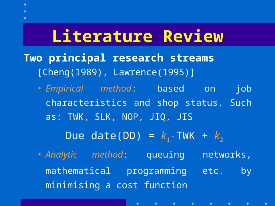
Literature ReviewTwo principal research streams

[Cheng(1989), Lawrence(1995)]

• Empirical method: based on job characteristics and

shop status. Such as: TWK, SLK, NOP, JIQ, JIS

Due date(DD) = k1TWK + k2

• Analytic method: queuing networks, mathematical

programming etc. by minimising a cost function

Literature Review

Limitation of above research

• Both focus on job shop situations

• Empirical - rely on simulation, time consuming

in stochastic systems

• Analytic - limited to “small” problems

Appr. procedure for product DDAnalytical / numerical

method

Moments of two-stageleadtime

Approximate leadtimedistribution

Product due dateplanning

Appr. procedure for stage DD

Analytical / numericalmethod

Moments of two-stageleadtime

Approximate leadtimedistribution

Stage due dateplanning

• Product structure

Simple Two Stage System

ComponentManufacturing

Assembly

11 12 1n

1

Planned start time S1, S1i

component 11

component 12

component 1n

assembly proc. time

assembly proc. time

component 1n

S 1S 11

S 12

S 1n

... ...

• Holding cost at subsequent stage• Resource capacity limitation• Reduce variability

Minimum processing time M1

Prob. density func.(PDF) Cumul. distr. func.(CDF) • Big variance may result in negative operation times

Analytical Result• CDF of leadtime W is:

FW(t) = 0, t<M1+S1;

FW(t) = F1(M1) FZ(t-M1) + F1FZ, t M1 + S1.where

F1 CDF of assembly processing time;

FZ CDF of actual assembly start time;

FZ(t)= 1n F1i(t-S1i)

convolution operator in [M1, t - S1];

F1FZ= F1(x) FZ(x-t)dx

Leadtime Distribution EstimationComplex product structure approximate method

Assumptions normally distributed processing times approximate leadtime by truncated normal distribution

(Soroush, 1999)

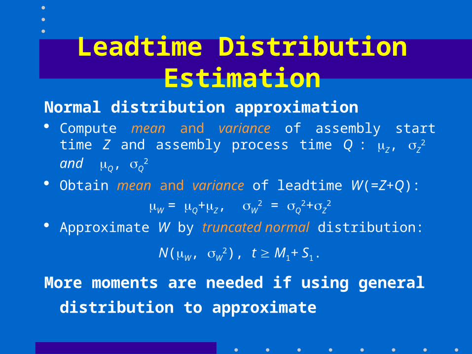
Leadtime Distribution Estimation

Normal distribution approximation Compute mean and variance of assembly start time Z and

assembly process time Q : Z, Z2 and Q, Q

2

Obtain mean and variance of leadtime W(=Z+Q):

W = Q+Z, W2 = Q

2+Z2

Approximate W by truncated normal distribution:

N(W, W2), t M1+ S1.

More moments are needed if using general

distribution to approximate

Due Date Planning• Achieve a specified probability

DD* by N(0, 1)

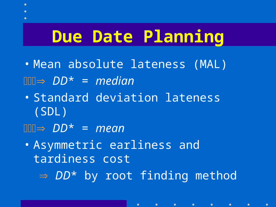
Due Date Planning

• Mean absolute lateness (MAL)

DD* = median

• Standard deviation lateness (SDL)

DD* = mean

• Asymmetric earliness and tardiness cost

DD* by root finding method

Industrial Case Study• Product structure

17 components 17 components

Stage 1

Stage 2

Stage 3

Stage 4

Stage 5

Stage 6 … … … …

System parameters setting

• normal processing times• at stage 6: =7 days for 32 components,

=3.5 days for the other two.

• at other stages : =28 days

• standard deviation: = 0.1

• backward scheduling based on mean data• planned start time: 0 for 32 components and 3.5 for

other two.

Simulation histogram & Appr. PDF

Simulation histogram & Appr. PDF

Product Due Date

Prob. 0.50 0.60 0.70 0.80 0.90

due simu. 150.86 152.11 153.44 155.26 157.46

date appr. 151.66 152.85 154.12 155.61 157.72

• Simulation verification for product due date to achieve specified probability

Stage Due Dates

Stage 6 5 4 3 2 1

Due Date 8 40 72 104 135 167

Prob.achievedin simul.

90.6%

88.3%

90.8%

89.9%

91.8%

89.9%

• Simulation verification for stage due dates to achieve 90% probability

Discussion

• Minimum processing time

• Production plan

• Stage due date

Conclusion

• Complex product systems with uncertainty

• A procedure to estimate leadtime distribution

• Approximate method to set due dates

• Used to design planned start times

Further Work

• Skewed processing times

• Using more general distribution to

approximate, like -type distribution

• Resource constraint systems