Embed Size (px)
Citation preview

DSGE models: problems and some personalsolutions
Fabio Canova
EUI and CEPR
March 2014

Outline of the talk
• Identification problems.
• Singularity problems.
• External information problems.
• Data mismatch problems.
• Model evaluation problems.

References
Canova, F. (2009) How much structure in empirical models, in Mills and Patterson, (eds.) Palgrave
Handbook of Econometrics II, Palgrave.
Canova, F. (2007) Methods for Applied Macroeconomic Research, Princeton University Press.
Canova, F. (2012) Bridging DSGE models and raw data, manuscript.
Canova, F. and Ferroni, F. (2011) Multiple filtering devices for estimating cyclical DSGE models, Quanti-
tative Economics.
Canova, F. and Paustian, M. (2011) Measurement with some theory: using sign restrictions to evaluate
business cycles models, Journal of Monetary Economics.
Canova, F. and Sala, L. (2009) Back to square one: identification issues in DSGE models, Journal of
Monetary Economics.
Canova, F., Ferroni, C. Matthes (2014) Choosing the variables to estimate DSGE models, Journal of Applied
Econometrics.
All available at http://www.eui.eu/Personal/Canova/

What are DSGE models?
[+1 + + −1 ++1 + ] = 0 (1)
+1 − − = 0 (2)
Their stationary (log-linearized) rational expectation solution is:
= +−1 + −1 + (3)
= −1 + (4)
where are functions of and are the
structural parameters.

Benchmark in academics for:
- Understanding generation and propagation of business cycles.
- Conduct policy analyses.
Popular in central banks/policy circles because:
- Give a coherent story with all general equilibrium interactions.
- Give sharp and easy to communicate optimal policy actions.
- Can use them to forecast (OK when compared to time series models).
- Same language and same tools of academics - no misunderstandings.

Big drive to use Bayesian methods. Why?
- Existence of specialized software (Dynare) makes estimation easy.
- Can incorporate external information in the form of a prior - sophisticated
interval calibration.
- Classical estimates make sense only if the model is (asymptotically) the
DGP of the data up to a set of serially correlated errors. Posterior estimates
valid even when the model is not the DGP; and in small samples.
- Estimates make (economic) sense (not always the case with classical
methods).

General problems
- The likelihood of a DSGE is generally ill-behaved.

- Severe population identification difficulties.
- Misspecification.
- Fundamental mismatch about the nature of the models and the data.
- General singularity issues.

1. Identification issues
• Crucial DSGE parameters face identification problems.
• Problems are compounded in large scale models.
• Standard fixup are problematic.
• Bayesian methods are a mixed blessing.

Where could identification problems be?
• The solution mapping, linking the to the (reduced form) coefficients ofthe decision rule (, etc.) Additional problem: numerical solution.
• The objective function mapping, linking the solution to the populationobjective function (likelihood or posterior) - multiple peaks, flat areas.
• The data mapping, linking the population to the sample objective func-tions - small samples, error in variables, omitted variables.

Example 1: Observational equivalence, under-identification
and weak identification
= 1 + 1+1 + 2( −+1) + 1 (5)
= 2 + 3+1 + 4 + 2 (6)
= 3 + 5+1 + 3 (7)
where is the output gap, the inflation rate, the nominal interest rate, 1 2 3iid contemporaneously uncorrelated shocks and 1 2 3 are constants. The solution is:⎡⎣
⎤⎦ =⎡⎣ 1
23
⎤⎦+⎡⎣ 1 0 2
4 1 240 0 1
⎤⎦⎡⎣ 123
⎤⎦ ≡ + (8)
where () function of .

• 1 3 5 disappear from the dynamics.
• Observational equivalence: can’t study determinate vs. indeterminatesolutions; Sticky vs. non-sticky information.
• Different shocks identify different parameters.
• ML and distance function (based on impulse responses) have differentidentification properties. Steady state information matters!

Example 2: RBC model: Distortions
0 0.2 0.4 0.6 0.8 10
0.1
0.2
0.3
0.4
0.5
0.6
0.7
0.8
0.9
1
a4
a2Distance − e3 shock
0.1
0.05
0.010.001
0 0.2 0.4 0.6 0.8 10
0.1
0.2
0.3
0.4
0.5
0.6
0.7
0.8
0.9
1
a4
a2
Distance − low a2
0.1
0.05
0.010.001
0 0.2 0.4 0.6 0.8 10
0.1
0.2
0.3
0.4
0.5
0.6
0.7
0.8
0.9
1
a4
a2
Likelihood
100
10
1
0 0.2 0.4 0.6 0.8 10
0.1
0.2
0.3
0.4
0.5
0.6
0.7
0.8
0.9
1
a4
a2
Likelihood − wrong calibration
100
10
1
0.5 1 1.50
0.1
0.2
0.3
0.4
0.5
0.6
0.7
0.8
0.9
k3
a3
Likelihood
10010
1
0.5 1 1.50
0.1
0.2
0.3
0.4
0.5
0.6
0.7
0.8
0.9
k3
a3
Posterior
100
10
1
Distance function, Likelihood and Posterior.

• Identification is local (depends on true parameter values, if they exist).
• Calibrating difficult parameters may lead to gross mistakes.
• Prior can cover up identification problems (convexify the likelihood).

Example 3: Standard NK model with frictions: wrong inference
Case 1 0.887 0.862 0.620 0.221max 0.979 0.910 0.884 0.980median 0.845 0.515 0.641 0.657min 0.034 0.015 0.028 0.009Case 5 0.887 0.862 0.620 0.221max 0.989 0.989 0.986 0.987median 0.873 0.406 0.906 0.563min 0.046 0.001 0.122 0.008
Population intervals producing objective functions in the 0.01 contour.
- Wrong inference (confuse price and wage indexation).
- Wrong policy advise.

What can one do to solve problems?
- Always use all possible information (add steady states or the covariance
matrix of the shocks information). Limited information procedures likely
to have worse identification properties.
- Partial identification problems (ridges) difficult to deal with. Need to
reparametrize the model.
- Add sufficient internal dynamics (see Sargent 1978).

2. Singularity issues
- DSGE models typically singular. Does it matter which variables are used
to estimate the parameters? Yes.
i) Omitting relevant variables may lead to distortions in parameter esti-
mates.
ii) Adding variables may improve the fit, but also increase standard errors
if added variables are irrelevant.
iii) Different variables may identify different parameters (e.g. with aggre-
gate consumption data and no data on who own financial assets may be
very difficult to get estimate the share of rule-of-thumb consumers).

Recall solution of example 1:⎡⎢⎣
⎤⎥⎦ =⎡⎢⎣ 1 0 24 1 240 0 1
⎤⎥⎦⎡⎢⎣ 123
⎤⎥⎦+
iv) Likelihood function may change shape depending on the variables used.
Multimodality may be present if important variables are omitted (e.g. if
is excluded in above example).
- Levin et al. (2005, NBER macro annual): habit in consumption is 0.30;
Fernandez Villaverde and Rubio Ramirez (2008, NBER macro annual):
habit in consumption is 0.88. Same model and same sample. But use
different data to estimate the model!

Guerron Quintana (2010); use Smets and Wouters model and different
combinations of observable variables.
Parameter Wage stickiness Price Stickiness Slope PhillipsData Median (90%) Median (90%) Median (90%)Basic 0.62 (0.54,0.69)0.82 (0.80, 0.85)0.94 (0.64,1.44)
Without C 0.80 (0.73,0.85)0.97 (0.96, 0.98)2.70 (1.93,3.78)Without Y 0.34 (0.28,0.53)0.85 (0.84, 0.87)6.22 (5.05,7.44)Without C,W0.57 (0.46,0.68)0.71 (0.63, 0.78)2.91 (1.73,4.49)Without R 0.73 (0.67,0.78)0.81 (0.77, 0.84)0.74 (0.53,1.03)


Solutions:
• Solve out variables from the FOC before you compute the solution.
Which variables do we solve out? Problem: solution is a restricted VARMA
- not a VAR.
• Add measurement errors to complete probability space. How many?
Where? Need to restrict time series properties of measurement error (see
Altug,1989, Ireland, 2004).
• Invent structural shocks. Nuisance parameter problem!

Canova, Ferroni and Matthes (2013):
• Use formal criteria to select variables to be used in estimation
1) Choose vector that maximize the identifiability of relevant parameters.
Use Komunjer and Ng (2011) tools. Compare the curvature of the convo-
luted likelihood in the singular and the non-singular systems in the dimen-
sions of interest to eliminate ties and explore weak identification issues
2) Choose vector that minimize the information loss going from the larger
scale to the smaller scale system. Information loss is measured by
(
−1 ) =L(| −1 )L(| −1 )
(9)

where L(| 1) is the likelihood of which are defined by
= + (10)
= + (11)
is an iid convolution error, the original set of variables and the
j-th subset of the variables producing a non-singular system.
• Apply procedures to SW model driven with 4 shocks and 7 potential
observables.

Unrest SW RestrSW Restr andVector Rank(∆) Rank(∆) Sixth Restr
186 188 185 188 185 188 185 188 185 188 185 188 185 188 185 187...
183 187 183 187 183 187 183 187 183 186Ideal 189 189
Rank conditions for all combinations of variables in the unrestricted SW model (columns 2) and in the
restricted SW model (column 3), where = 0025, = = 10, = 15 and = 018. The fourth
columns reports the extra parameter restriction needed to achieve identification; a blank space means that
there are no parameters able to guarantee identification.

0.65 0.7 0.75
−10
0
10
h = 0.710.55 0.6 0.65 0.7 0.75
−40
−20
0
ξp = 0.65
0.35 0.4 0.45 0.5 0.55
−10
0
10
γp = 0.47
1.6 1.8 2 2.2
−10
−5
0
5
10
σl = 1.92
1.8 2 2.2
−20
0
20
ρπ = 2.030 0.1 0.2
−50
0
50
ρy = 0.08
DGPoptimal
Likelihood curvature

Basic T=1500 Σ = 001 ∗ Order Vector Relative Info Vector Relative info Vector Relative Info
1 ( ) 1 ( ) 1 ( ) 12 ( ) 0.89 ( ) 0.87 ( ) 0.863 ( ) 0.52 ( ) 0.51 ( ) 0.514 ( ) 0.5 ( ) 0.5 ( ) 0.5
Ranking based on the information statistic. The first two column present the results
for the basic setup, the next six columns the results obtained altering some nuisance
parameters. Relative information is the ratio of the () statistic relative to the best
combination.

• How different are good and bad combinations?
- Simulate 200 data points from the model with four shocks and estimatestructural parameters using
(1) Model A: 4 shocks and ( ) as observables (best rank analysis).
(2) Model B: 4 shocks and ( ) as observables (best information analysis).
(3) Model Z: 4 shocks and ( ) as observables(worst rank analysis).
(4) Model C: 4 structural shocks, three measurement errors and ( ) as
observables.
(5) Model D: 7 structural shocks (add price and wage markup and preference shocks)
and ( ) as observables.

True Model A Model B Model Z Model C Model D 0.95 ( 0.920 , 0.975 ) ( 0.905 , 0.966 ) ( 0.946 , 0.958) ( 0.951 , 0.952 ) ( 0.939 , 0.943)* 0.97 ( 0.930 , 0.969 ) ( 0.930 , 0.972 ) ( 0.601 , 0.856)* ( 0.970 , 0.971 ) ( 0.970 , 0.972 ) 0.71 ( 0.621 , 0.743 ) ( 0.616 , 0.788 ) ( 0.733 , 0.844)* ( 0.681 , 0.684)* ( 0.655 , 0.669)* 0.51 ( 0.303 , 0.668 ) ( 0.323 , 0.684 ) ( 0.010 ,0.237 )* ( 0.453 , 0.780 ) ( 0.114 , 0.885)* 1.92 ( 1.750 , 2.209 ) ( 1.040 , 2.738 ) ( 0.942 , 2.133) ( 1.913 , 1.934 ) ( 1.793 , 1.864)* 1.39 ( 1.152 , 1.546 ) ( 1.071 , 1.581 ) ( 1.367 , 1.563) ( 1.468 , 1.496)* ( 1.417 , 1.444)* 0.71 ( 0.593 , 0.720 ) ( 0.591 , 0.780 ) ( 0.716 , 0.743 ) (0.699 , 0.701)* ( 0.732 , 0.746)* 0.73 ( 0.402 , 0.756 ) (0.242, 0.721)* ( 0.211 ,0.656 )* ( 0.806 , 0.839)* 0.65 ( 0.313 , 0.617)* ( 0.251 , 0.713 ) ( 0.512 , 0.616 )* ( 0.317 , 0.322)* ( 0.509 , 0.514)* 0.59 ( 0.694 , 0.745 ) ( 0.663 , 0.892)* ( 0.532 ,0.732 ) ( 0.728 , 0.729)* ( 0.683 , 0.690)* 0.47 ( 0.571 , 0.680)* ( 0.564 , 0.847)* ( 0.613 , 0.768 )* ( 0.625 , 0.628)* ( 0.606 , 0.611)* 1.61 ( 1.523 , 1.810 ) ( 1.495 , 1.850 ) ( 1.371 , 1.894 ) ( 1.624 , 1.631)* ( 1.654 , 1.661)* 0.26 ( 0.145 , 0.301 ) ( 0.153 , 0.343 ) ( 0.255 , 0.373 ) ( 0.279 , 0.295)* ( 0.281 , 0.306)* 5.48 ( 3.289 , 7.955 ) ( 3.253 , 7.623 ) ( 2.932 , 7.530 ) ( 11.376 , 13.897)* ( 4.332 , 5.371)* 0.2 ( 0.189 , 0.331 ) ( 0.167 , 0.314 ) ( 0.136 , 0.266 ) ( 0.177 , 0.198)* ( 0.174 , 0.199)* 2.03 ( 1.309 , 2.547 ) ( 1.277 , 2.642 ) ( 1.718 , 2.573 ) ( 1.868 , 1.980)* ( 2.119 , 2.188)* 0.08 (0.001 , 0.143 ) ( 0.001 , 0.169 ) ( 0.012 , 0.173) ( 0.124 , 0.162)* 0.87 ( 0.776 , 0.928 ) ( 0.813 , 0.963 ) ( 0.868 , 0.916 ) ( 0.881 , 0.886)*∆ 0.22 ( 0.001 , 0.167)* (0.010, 0.192)* ( 0.130 ,0.215 )* (0.235 , 0.244)* 0.46 ( 0.261 , 0.575 ) ( 0.382 , 0.460 ) ( 0.420 ,0.677 ) ( 0.357 , 0.422)* ( 0.386 , 0.455)* 0.61 ( 0.551 , 0.655 ) ( 0.551 , 0.657 ) ( 0.071 ,0.113 ) ( 0.536 , 0.629 ) ( 0.585 , 0.688)* 0.6 ( 0.569 , 0.771 ) ( 0.532 , 0.756 ) ( 0.503 ,0.663 ) ( 0.561 , 0.660 ) ( 0.693 , 0.819)* 0.25 ( 0.100 , 0.259 ) ( 0.078 , 0.286 ) ( 0.225 ,0.267 ) ( 0.226 , 0.265 ) ( 0.222 , 0.261 )

10 20 30 400
0.2
0.4
0.6
y
10 20 30 40
−0.2
−0.15
−0.1
−0.05
0
c
10 20 30 40
−1
−0.5
0i
10 20 30 40−0.04
−0.02
0
0.02
0.04
w
10 20 30 400
0.1
0.2
0.3
0.4
h
10 20 30 400
0.01
0.02
π
10 20 30 400
0.01
0.02
0.03
0.04
r
trueModel A InfModel A SupModel Z InfModel Z Sup
Responses to a goverment spending shock

10 20 30 40
0.2
0.4
0.6
y
10 20 30 40
0.1
0.2
0.3
0.4
c
10 20 30 400
0.5
1
1.5
i
10 20 30 40
0.05
0.1
0.15
0.2
0.25
0.3
w
10 20 30 40
−0.3
−0.2
−0.1
0
0.1
h
10 20 30 40
−0.06
−0.04
−0.02
0
π
10 20 30 40
−0.08
−0.06
−0.04
−0.02
0r
trueModel B InfModel B SupModel C InfModel C Sup
Responses to a technology shock

0 5 10 15 20 25 30 35 40−0.2
−0.15
−0.1
−0.05
0
0.05
y0 5 10 15 20 25 30 35 40
−20
−15
−10
−5
0
5x 10
−4
0 5 10 15 20 25 30 35 40−0.1
−0.05
0
0.05
h0 5 10 15 20 25 30 35 40
−2
−1
0
1x 10
−3
0 5 10 15 20 25 30 35 40−0.1
0
0.1
0.2
π0 5 10 15 20 25 30 35 40
−2
0
2
4x 10
−3
0 5 10 15 20 25 30 35 40−0.02
0
0.02
0.04
r
0 5 10 15 20 25 30 35 40−5
0
5
10x 10
−4
SWEst
Responses to an price markup shock

3. Practical issues
• How do you estimate DSGE models when:
a) the variables are mismeasured relative to the model quantities?
b) there are multiple observables that correspond to model quantities?
c) have information about variables not included in the model.

For a): add measurement errors to model variables
Observables 1. Model based quantities () = , is a selection
matrix.
1 = () + (12)
where is iid measurement error.
- Estimate 2 jointly.
- Use properties of 2 to assess misspecification.

- How do you measure hours? Use establishment survey series? Householdsurvey series? Employment?

• For b) Let 2 be a ×1 vector of observables and () be of dimension × 1 where dim(N) dim(k). Then:
2 = Λ1() + 1 (13)
where the first row of Λ1 is normalized to 1 and is iid measurement
error.
- Estimate 2Λ1 jointly. Λ1 = 2 measures the relative infor-
mational content of various indicators.
- Can reduce the noise (var[()] will be asymptotically of the order 1
time the variance obtained when only one indicator is used (see Stock and
Watson (2002)).
- Estimates of more precise, see Justiniano et al. (2012).

Many cases fit in c):
- Proxy measures for the unobservable states: commodity prices used asproxies for future inflation shocks, stock market shocks used as proxies forfuture technology shocks, see Beaudry and Portier (2006).
- Sometimes we have survey data, conjunctoral information providing in-formation for unobserved states (e.g. business cycles).
- Mixed frequency data
Specification:
3 = Λ2 + 2 (14)
where Λ2 is unrestricted and a ×1 vector of states and 3 are measuresof future states (inflation, output) at different horizons, financial informa-tion (oil prices, stock prices, term structure, etc.) or quarterly sampling ofe.g. monthly observation (see Foroni and Marcellino (2013)).

A. Tryphonides: How external information can contribute to structural
analysis?


4. Data mismatch issues
- Most of models available for policy are stationary and cyclical.
- Data is close to non-stationary; it has trends and displays breaks.
- How to we match models to the data?
a) Detrend actual data: the model is a representation for detrended data.
Problem: which detrended data is the model representing?

1965 1970 1975 1980 1985 1990 1995 2000 2005−8
−6
−4
−2
0
2
4
6GDP
LTHPFODBKCF

b) Take ratios in the data and in the model - will get rid of trends if
variables in the ratio are cointegrated. Problem: data does not seem to
satisfy balanced growth.
1950:1 1962:2 1974:4 1986:2 1998:4
0.57
0.58
0.59
0.6
0.61
0.62
0.63
c/y re
al
1950:1 1962:2 1974:4 1986:2 1998:40.04
0.06
0.08
0.1
0.12
0.14
i/y re
al
1950:1 1962:2 1974:4 1986:2 1998:40.52
0.54
0.56
0.58
0.6
0.62
0.64
c/y n
omina
l
1950:1 1962:2 1974:4 1986:2 1998:40.08
0.1
0.12
0.14
0.16
i/y n
omina
lReal and nominal Great ratios in US, 1950-2008.

c) Build-in a trend into the model. Detrend the data with model-based
trend. Problems: Specification of the trend is arbitrary (deterministic?
stochastic?); where you put the trend (TFP? preference?) matters for
estimation and inference.
• General problem: statistical definition of a cycle is different from the
economic definition. All statistical approaches are biased, even in large
samples.

0 0.5 1 1.5 2 2.5 3 3.50
1000
2000
3000
4000
5000
6000
7000
8000
9000
10000Ideal Situation
datacycle 1
Ideal case

0 0.5 1 1.5 2 2.5 3 3.50
1000
2000
3000
4000
5000
6000
7000
8000
9000
10000Non−cyclical has power at BC frequencies
datacycle 3
General case
- In developing countries most of cyclical fluctuations driven by trends(permanent shocks), see Aguiar and Gopinath (2007).

Example 4: The log linearized equilibrium conditions of basic NK model are:
= −
1− ( − −1) (15)
= + (1− ) (16)
= − + (17)
= −1 + (1− )( + ) + (18)
= (+1 + − +1) (19)
= ( + − + ) + +1 (20)
= −1 + (21)
where =(1−)(1−)
1−1−+, is the Lagrangian on the consumer budget constraint,
is a technology shock, a preference shock, is an iid monetary policy shock and
an iid markup shock.
Estimate this model with different detrending transformations. Do we get
different estimates?


2 4 6 8 10 12 14−0.1
0
0.1
0.2
0.3
y t
Preference Shocks
2 4 6 8 10 12 140
0.2
0.4
0.6
wt
2 4 6 8 10 12 140
0.05
0.1
0.15
0.2
π t
2 4 6 8 10 12 140
0.05
0.1
r t
2 4 6 8 10 12 140
0.5
1
Technology Shocks
2 4 6 8 10 12 14
−1
0
1
2 4 6 8 10 12 14
−0.2
−0.1
0
0.1
0.2
2 4 6 8 10 12 14
−0.4
−0.2
0
0.2
LT HP FOD BP Ratio 1 Ratio 2
Estimated impulse responses.

Two approaches to deal with mismatch problem:
1) Data-rich environment: Canova and Ferroni (2011). Let be the
actual data filtered with method and = [1
2 ]. Assume:
= 0 + 01() + (22)
where = 0 1 are matrices of parameters, measuring the bias and
correlation between the filter data and model based quantities (); are measurement errors and the structural parameters.
- Same setup as before: model based quantities are non-observable.
- Jointly estimate 2 and ’s. Can obtain a more precise estimates of
the unobserved () if measurement error is uncorrelated across filtering
methods.

2) Bridge cyclical model and the data (Canova, 2012)).
= + + () + (23)
where ≡ − ( ) the log demeaned vector of observables, =
− ( ), is the non-model component, () ≡ [ ]
0, is
a selection matrix, is the model based component, is a iid (0Σ)
(measurement) noise, () and are mutually orthogonal.
- Model (linearized) solution:
= ()−1 + () (24)
= ()−1 +() (25)
+1 = () + +1 (26)
() () () () functions of the structural parameters =
(1 ), = − ; = − ; and are the disturbances,
are the steady states of and .

-Non model-based component:
= 1−1 + −1 + ∼ (0Σ2) (27)
= 2−1 + ∼ (0Σ2) (28)
Σ2 0 and Σ2 = 0, is a vector of I(2) processes. 1 = 2 = Σ2 = 0,
and Σ2 0, is a vector of I(1) processes. 1 = 2 = Σ2 = Σ2 = 0,
is deterministic. 1 = 2 = Σ2 0 and Σ2 0 and22is large, is
smooth ( as in HP). 1 6= 2 6= or both, non-model based component
has power at particular frequencies
- Jointly estimate structural and non-structural parameters (1 2ΣΣ).

Advantages of suggested approach:
• No need to take a stand on the properties of the non-cyclical componentand on the choice of filter to tone down its importance - specification errors
and biases limited.
• Estimated cyclical component not localized at particular frequencies ofthe spectrum.
• Account for trend uncertainty in estimates of .
• Provides a measure of model misspecification.

DGP1: Trend is importantTrue value LT HP FOD BP Ratio1Flexible
0.50 0.04 0.08 0.00 0.11 0.05 0.04 0.70 0.00 0.00 0.00 0.01 0.07 0.10 0.30 0.00 0.04 0.00 0.06 0.04 0.06 0.70 0.05 0.05 0.01 0.06 0.13 0.01 1.50 0.00 0.00 0.00 0.01 0.02 0.00 0.40 0.17 0.20 0.17 0.19 0.15 0.00 0.75 0.03 0.04 0.03 0.03 0.02 0.03 0.50 0.00 0.04 0.00 0.00 0.00 0.07 0.80 0.03 0.05 0.00 0.05 0.00 0.05 1.12 1.60 0.45 3.89 0.64 8.79 1.00 0.50 1.47 0.01 3.18 0.03 0.02 0.16 0.10 1.37 0.03 3.75 0.03 0.00 0.00 1.60 13.1418.8117.6838.52 38.36 1.94
Total1 0.30 0.40 0.21 0.48 0.49 0.24Total2 17.9119.7928.7139.75 47.66 3.45
MSE. In DPG1 there is a unit root component to the preference shock and
= [11 19].

DGP2: Trend unimportantTrue value LT HP FOD BP Ratio1Flexible
0.50 0.04 0.11 0.17 0.12 0.12 0.06 0.70 0.01 0.00 0.00 0.03 0.08 0.17 0.30 0.00 0.05 0.00 0.06 0.02 0.07 0.70 0.05 0.05 0.04 0.05 0.13 0.02 1.50 0.00 0.00 0.00 0.00 0.01 0.00 0.40 0.16 0.21 0.08 0.19 0.15 0.00 0.75 0.03 0.04 0.02 0.05 0.04 0.03 0.50 0.00 0.04 0.00 0.00 0.01 0.08 0.80 0.04 0.05 0.03 0.03 0.00 0.06 1.12 10.41 0.87 2.80 0.69 9.43 0.97 0.50 9.15 0.06 1.91 0.06 0.01 0.17 0.10 9.35 0.00 1.05 0.03 0.00 0.00 1.60 10.4120.7220.3357.03 40.17 1.90
Total1 0.29 0.46 0.32 0.51 0.55 0.35Total2 39.6522.2026.4458.34 50.17 3.54
MSE. In DGP2 all shocks are stationary but there is measurement error and
=
[009 011] The MSE is computed using 50 replications.

- The true and estimated log spectrum and ACF close.
- Both true and estimate cyclical components have power at all frequencies.

5 10 150
0.1
0.2Preference
y t
5 10 150
0.1
0.2Technology
5 10 15−0.2
−0.1
0Monetary Policy
5 10 15−2
−1
0x 10
−3Markup
5 10 15−0.2
0
0.2
ω t
5 10 15−2
−1
0
5 10 15−2
−1
0
5 10 15−0.04
−0.02
0
5 10 150
0.01
0.02
π t
5 10 15−0.4
−0.2
0
5 10 15−0.1
−0.05
0
5 10 15−0.02
0
0.02
5 10 150
0.02
0.04
r t
5 10 15−0.4
−0.2
0
5 10 15−1
0
1
5 10 15−0.02
0
0.02
True Estimated
Model based IRF, true and estimated.
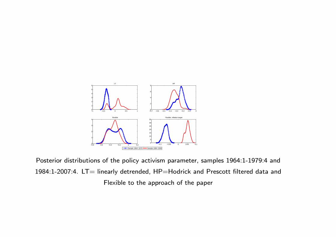
−1 −0.5 0 0.5 10
1
2
3
4
5
6LT
−0.7 −0.6 −0.5 −0.4 −0.3 −0.2 −0.1 00
2
4
6
8HP
−0.8 −0.6 −0.4 −0.2 0 0.20
1
2
3
4Flexible
−0.1 −0.05 0 0.05 0.10
5
10
15
20
25
30
35Flexible, inflation target
Sample 1964−1979 Sample 1984−2005
Posterior distributions of the policy activism parameter, samples 1964:1-1979:4 and
1984:1-2007:4. LT= linearly detrended, HP=Hodrick and Prescott filtered data and
Flexible to the approach of the paper

LT FOD FlexibleOutput InflationOutput InflationOutput Inflation
TFP shocks 0.01 0.04 0.00 0.01 0.01 0.19Gov. expenditure shocks 0.00 0.00 0.00 0.00 0.00 0.02Investment shocks 0.08 0.00 0.00 0.00 0.00 0.05
Monetary policy shocks 0.01 0.00 0.00 0.00 0.00 0.01Price markup shocks 0.75(*) 0.88(*) 0.91(*) 0.90(*) 0.00 0.21Wage markup shocks 0.00 0.01 0.08 0.08 0.03 0.49(*)Preference shocks 0.11 0.04 0.00 0.00 0.94(*) 0.00
Variance decomposition at the 5 years horizon, SW model. Estimates are obtained using
the median of the posterior of the parameters. A (*) indicates that the 68 percent highest
credible set is entirely above 0.10. The model and the data set are the same as in Smets
Wouters (2007). LT refers to linearly detrended data, FOD to growth rates and Flexible
to the approach this paper suggests.

5. Evaluation problems
- Validation problematic when the model is not the DGP of the data.
Standard econometric procedures inapplicable.
- Bridging procedure (Canova, 2012) can be used to measure how much
the model leaves unexplained without requiring the model to be the DGP.
Del Negro and Schorfheide (2004), (2006), Del Negro, et. al. (2006)
• Model can be used as a prior for the data.
• Can verify the quality of model’s restrictions by checking how much
simulated data must be added to a VAR to improve its fit.

Problems:
1) Condition on a single model. What if the model is wrong?
2) Look at the model as a whole: can’t measure discrepancy in one equa-
tion.
3) Not much to say about cyclical properties of the model.
Canova and Paustian (2011): address problems 1) and 2).

Basic idea:
- Find a set of robust dynamic implications in the model.
- Impose some of them on the data to identify shocks.
- Compare other dynamics implications of model and data in response to
robustly identified shocks.
- Use qualitative rather than quantitative evaluation. Can make the eval-
uation probabilistic.

Results with experimental data
- Can recognize qualitative features of the DGP with high probability.
- Can separate models which are close to each other with high probability.
- Can get a good handle of quantitative features of DGP if:
a) Restrictions are abundant (can’t be too agnostic).
b) Identified shocks have ”relative” large variance.
- Good even in small samples; median response tracks true one well.

Measuring the effects of government spending on consumption
- Models predict that consumption falls after increased government spend-
ing: negative wealth effect.
- VAR evidence generally the opposite: Blanchard and Perotti (2002),
Fatas and Mihov (2001), Perotti (2007), Pappa (2008).
- Gali et al. (2007): sticky prices and non-Ricardian consumers can produce
a rise in consumption following a government spending shock.
- Derive robust restrictions from this class of models. Check if conditioning
on the class of models, consumption increases or falls. (Test of sticky price
setup plus presence of rules of thumb consumers).

Robust restrictions: Gali et al (2007)
markupmonetaryspendingtechnology ? ? + - - - ? ? ? - + - - - + + - - + - ? ? - + - - ? +
Signs of impact response (105 draws, 95 % bands).

Question: Can the procedure recover the truth?
2 4 6 8 10 12 14 16 18 20 22 24
−0.8
−0.6
−0.4
−0.2
0
λ = 0
2 4 6 8 10 12 14 16 18 20 22 24
−0.5
0
0.5
1
λ = 0.8
97.5th−percentilemedian
2.5th−percentiletrue response
Consumption responses to government spending shock.

U.S. data: 1954:1-2007:1.
- Estimate a 5 variable VAR, ( ).
- Data is in log differences (except inflation in log levels).
- Identify spending shock ( 0 0 0 0) and generic
technology shock ( 0 0 0 0)

5 10 15 200
0.05
0.1
0.15
0.2
0.25
labor
5 10 15 20
−1.5
−1
−0.5
0
0.5
1
investment
5 10 15 20
0.02
0.04
0.06
0.08
0.1
0.12
0.14
inflation
5 10 15 200
0.1
0.2
0.3
0.4
0.5
consumption
5 10 15 20
0.2
0.4
0.6
0.8
1
spending
16th−percentilemedian84th−percentile
Response to a government spending shock in U.S. data, 1954-2007

Future challanges
- Dealing with time variations in the structure.
- Dealing with generic misspecification.
- Dealing with non-linear frameworks
Large Thanks for your attention and patience!