Drude Model

for dielectric constant of metals.

• Conduction Current in Metals• EM Wave Propagation in Metals• Skin Depth• Plasma Frequency

Ref : Prof. Robert P. Lucht, Purdue University

Drude model

Drude model : Lorenz model (Harmonic oscillator model) without restoration force(that is, free electrons which are not bound to a particular nucleus)

Linear Dielectric Response of Matter

Conduction Current in MetalsConduction Current in Metals

2

2

:

v

:

e

The current density is definedCJ N e with units of

s m

Substituting in the equation of motion we obtain

dJ N eJ Edt m

γ

⎡ ⎤= − ⎢ ⎥−⎣ ⎦

⎛ ⎞+ = ⎜ ⎟

⎝ ⎠

r r

rr r

The equation of motion of a free electron (not bound to a particular nucleus; ),

( : relaxation time )

2

2

14

0

1 10

r r rr uur r uur

ee e e

C

md r dr dvm Cr eE m m v eEdt dtdt

s

γτ

τγ

−

=

= − − − ⇒ + = −

= ≈Lorentz model(Harmonic oscillator model)

If C = 0, it is called Drude model

Conduction Current in MetalsConduction Current in Metals

( ) ( )

( )( ) ( ) ( )

0 0

00 0 0

:

exp exp

:

expexp exp exp

Assume that the applied electric field and the conduction current density are given by

E E i t J J i t

Substituting into the equation of motion we obtain

d J i tJ i t i J i t J i t

dt

ω ω

ωγ ω ω ω γ ω

= − = −

⎡ ⎤−⎣ ⎦ + − = − − + −

r r r r

rr r r

( )

( )

( )

( )

2

0

2

0 0

2

exp

exp :

e

e

e

N e E i tm

Multiplying through by i t

N ei J Em

N eor equivalently i J Em

ω

ω

ω γ

ω γ

⎛ ⎞= −⎜ ⎟⎝ ⎠

+

⎛ ⎞− + = ⎜ ⎟

⎝ ⎠⎛ ⎞

− + = ⎜ ⎟⎝ ⎠

r

r r

r r

Local approximation to the current-field relation

Conduction Current in MetalsConduction Current in Metals( )

( )

( )

2 2

0 :

:

1 /

, 1,

e e

For static fields we obtain

N e N eJ E E static conductivitym m

For the general case of an oscillating applied field

J E E dynamic conductivityi

For very low frequencies the dyn

ω ω

ω

σ σγ γ

σ σ σω γ

ω γ

=

⎛ ⎞= = ⇒ = =⎜ ⎟⎝ ⎠

⎡ ⎤= = =⎢ ⎥−⎣ ⎦

<<

r r r

r r r

.

,,

amic conductivity is purely real andthe electrons follow the electric field

As the frequency of the applied field increases the inertia of electrons introducesa phase lag in the electron response to the field andthe dynamic conducti

( )

.

, 1,90 .

vity is complex

For very high frequencies the dynamic conductivity is purely imaginaryand the electron oscillations are out of phasewith the applied field

ω γ >>

°

Propagation of EM Waves in Metals

Propagation of EM Waves in Metals

( )

( )

22

2 2 20

22

2 2 20

' :

1 1

1 /

:

1 11 /

Maxwell s relations give us the following wave equation for metals

E JEc t c t

But J Ei

Substituting in the wave equation we obtain

E EEc t c i t

The wave equation is s

ε

σω γ

σε ω γ

∂ ∂∇ = +

∂ ∂

⎡ ⎤= ⎢ ⎥−⎣ ⎦

⎡ ⎤∂ ∂∇ = + ⎢ ⎥∂ − ∂⎣ ⎦

r rr

r r

r rr

( )

( )

0

22 20

20 0

:

exp

11 /

atisfied by electric fields of the form

E E i k r t

where

k i cc i

ω

σ ω μωω γ ε μ

⎡ ⎤= ⋅ −⎣ ⎦

⎡ ⎤= + =⎢ ⎥−⎣ ⎦

rr r r

0 ,0 ≠= JP

Skin DepthSkin Depth

( )

( )

2

22 0

0 02

00 0 0

0

:

exp1 / 2

, exp exp cos sin 12 4 4 4 2

2R I R

Consider the case where is small enough that k is given by

k i i ic i

Then k i i i i

k k n

ω

σ ω μω πσ ω μ σ ω μω γ

σ ω μπ π π πσ ω μ σ ω μ σ ω μ

σ ω μ

⎡ ⎤ ⎛ ⎞= + ≅ =⎢ ⎥ ⎜ ⎟− ⎝ ⎠⎣ ⎦

⎡ ⎤⎛ ⎞ ⎛ ⎞ ⎛ ⎞ ⎛ ⎞≅ = = + = +⎜ ⎟ ⎜ ⎟ ⎜ ⎟ ⎜ ⎟⎢ ⎥⎝ ⎠ ⎝ ⎠ ⎝ ⎠ ⎝ ⎠⎣ ⎦

= = =

%

( ) ( ) ( )

20

0

0 0

2 2

, :

exp exp exp exp

R I

I R R

cc k n

In the metal for a wave propagating in the z directionzE E k z i k z t E i k z t

σ μ σω ω ωε

ω ωδ

⎛ ⎞ = = =⎜ ⎟⎝ ⎠

−

⎛ ⎞= − − = − −⎡ ⎤ ⎡ ⎤⎜ ⎟⎣ ⎦ ⎣ ⎦⎝ ⎠

r r r

20

0

27 1 1 7

21 2:

5.76 10 5.76 10 0.66

I

cThe skin depth is given byk

C sFor copper the static conductivity m mJ m

εδ δσ ω μ σ ω

σ δ μ− −

= = =

−= × Ω = × → =

−

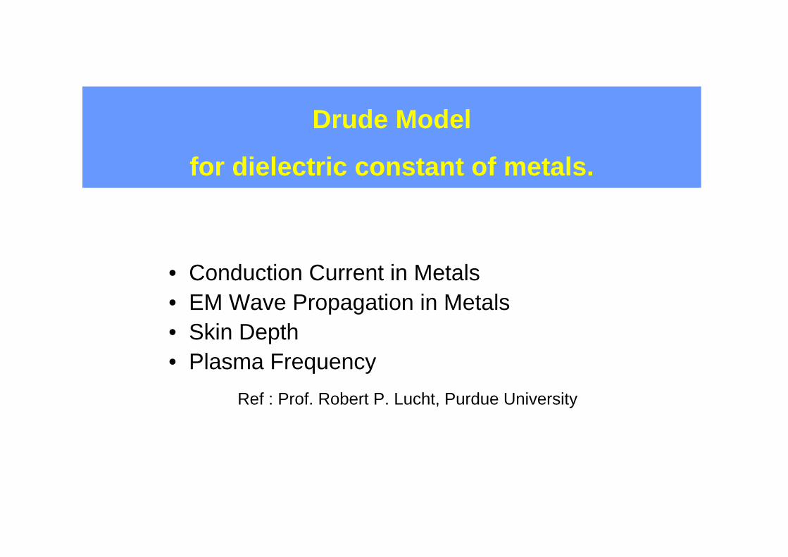
Plasma FrequencyPlasma Frequency

( )

( ) ( )

22 0

2

2 222 2 0 0

2

22 0

2

22 2 2

0

:

1 /

1 11 / 1 /

1

:

pe

Now consider again the general case

k ic i

c cc in k i iii i

cni

The plasma frequency is defined

N ec cm

σ ω μωω γ

σ μ σ μγω γω ω γ ω ω γ

γ σ μω ωγ

ω γ σ μ γγ

⎡ ⎤= + ⎢ ⎥−⎣ ⎦

⎧ ⎫ ⎧ ⎫⎪ ⎪ ⎪ ⎪= = + = +⎨ ⎬ ⎨ ⎬− −⎡ ⎤ ⎡ ⎤⎪ ⎪ ⎪ ⎪⎣ ⎦ ⎣ ⎦⎩ ⎭ ⎩ ⎭

= −+

⎛ ⎞= = ⎜ ⎟

⎝ ⎠

2

00

22

21

e

p

N em

The refractive index of the medium is given by

ni

με

ωω ωγ

=

= −+

If the electrons in a plasma are displaced from a uniform background of ions, electric fields will be built up in such a direction as to restore the neutrality of the plasma by pulling the electrons back to their original positions. Because of their inertia, the electrons will overshoot and oscillate around their equilibrium positions with a characteristic frequency known as the plasma frequency.

/ ( ) / : electrostatic field by small charge separation

exp( ) : small-amplitude oscillation

( ) ( ) 2 2 2

2 22

s o o o

o p

s p po o

E Ne x x

x x i t

d x Ne Nem e E mmdt

σ ε δ ε δ

δ δ ω

δ ω ωε ε

= =

= −

= − ⇒ − = − ⇒ ∴ =

Plasma Frequency Plasma Frequency

( / )

( )

2 2 22

2

22 2

2

1 11

1

o o

pR I

i c ccn ki i

n n ini

σ μ σ μ γω ω ω γ ω ωγ

ωω ωγ

⎛ ⎞= = + = −⎜ ⎟ − +⎝ ⎠

= + = −+

by neglecting , valid for high frequency ( ).

For , is complex and radiation is attenuated.

For , is real and radiation is not attenuated(transparent).

22

21 p

p

p

n

n

n

ωγ ω γ

ω

ω ω

ω ω

= − >>

<

>

Plasma Frequency Plasma Frequency

Plasma FrequencyPlasma Frequency

Born and Wolf, Optics, page 627.

ppc

cωπλλ 2

==

Plasma FrequencyPlasma Frequency

2

22

2

2 2

2 2

2 2 3 2

( )

( ) 1

( ) 2

1

R I

pR I

R I R I

p p

i n

n ini

n n i n n

i

ε ω ε ε

ωω ωγ

ω ω γω γ ω ωγ

= + =

= + = −+

= − +

⎛ ⎞ ⎛ ⎞= − +⎜ ⎟ ⎜ ⎟⎜ ⎟ ⎜ ⎟+ +⎝ ⎠ ⎝ ⎠

Dielectric constant of metal : Drude model

τγω 1=>>

2 2

2 3( ) 1/

p piω ω

ε ωω ω γ

⎛ ⎞ ⎛ ⎞= − +⎜ ⎟ ⎜ ⎟⎜ ⎟ ⎜ ⎟⎝ ⎠ ⎝ ⎠

Ideal case : metal as a free-electron gas

• no decay (infinite relaxation time)• no interband transitions

2

0 2( ) ( ) 1 pτγ

ωε ω ε ω

ω→∞→

⎛ ⎞⎯⎯⎯→ = −⎜ ⎟⎜ ⎟

⎝ ⎠

2

21 pr

ωε

ω= − 0

Note: SP is a TM wave!

Plasma waves (plasmons)

Plasmons

Plasmons in the bulk oscillate at ωp determined by the free electron density and effective mass

Plasmons confined to surfaces that can interact with light to form propagating “surface plasmon polaritons (SPP)”

Confinement effects result in resonant SPP modes in nanoparticles

+ + +

- - -

+ - +

k

Plasma oscillation = density fluctuation of free electrons

0

2

εω

mNedrude

p =

0

2

31

εω

mNedrude

particle =

Dispersion relation for EM waves in electron gas (bulk plasmons)

( )kω ω=

• Dispersion relation:

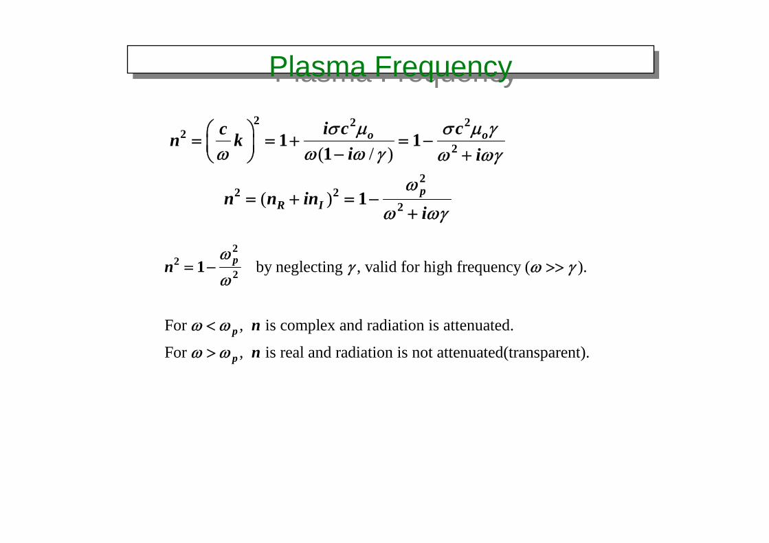
Dispersion relation of surface-plasmon for dielectric-metal boundaries

Dispersion relation for surface plasmon polaritons

TM waveεm

εd

xm xdE E= ym ydH H= m zm d zdE Eε ε=• At the boundary (continuity of the tangential Ex, Hy, and the normal Dz):

Z > 0

Z < 0

Dispersion relation for surface plasmon polaritons

zm zd

m d

k kε ε

=

xm xdE E=

ym ydH H=

xmmymzm EHk ωε=

ydd

zdym

m

zm HkHkεε

=

),0,( ziixii EiEi ωεωε −−),0,( yixiyizi HikHik−

xiiyizi EHk ωε=

xddydzd EHk ωε=

Dispersion relation for surface plasmon polaritons

• For any EM wave:2

2 2 2i x zi x xm xdk k k , where k k k

cωε ⎛ ⎞= = + ≡ =⎜ ⎟⎝ ⎠

m dx

m d

kc

ε εωε ε

=+

SP Dispersion Relation

1/ 2

' " m dx x x

m d

k k ikc

ε εωε ε

⎛ ⎞= + = ⎜ ⎟+⎝ ⎠

x-direction:

For a bound SP mode:

kzi must be imaginary: εm + εd < 0

k’x must be real: εm < 0

So,

1/ 22

' izi zi zi

m d

k k ikc

εωε ε

⎛ ⎞= + = ± ⎜ ⎟+⎝ ⎠

z-direction:2

2 2zi i xk k

cωε ⎛ ⎞= −⎜ ⎟⎝ ⎠

Dispersion relation:Dispersion relation for surface plasmon polaritons

' "m m miε ε ε= +

'm dε ε< −

2 22 2 zi i x x i x ik k i k k

c c cω ω ωε ε ε⎛ ⎞ ⎛ ⎞ ⎛ ⎞= ± − = ± − ⇒ >⎜ ⎟ ⎜ ⎟ ⎜ ⎟⎝ ⎠ ⎝ ⎠ ⎝ ⎠

+ for z < 0- for z > 0

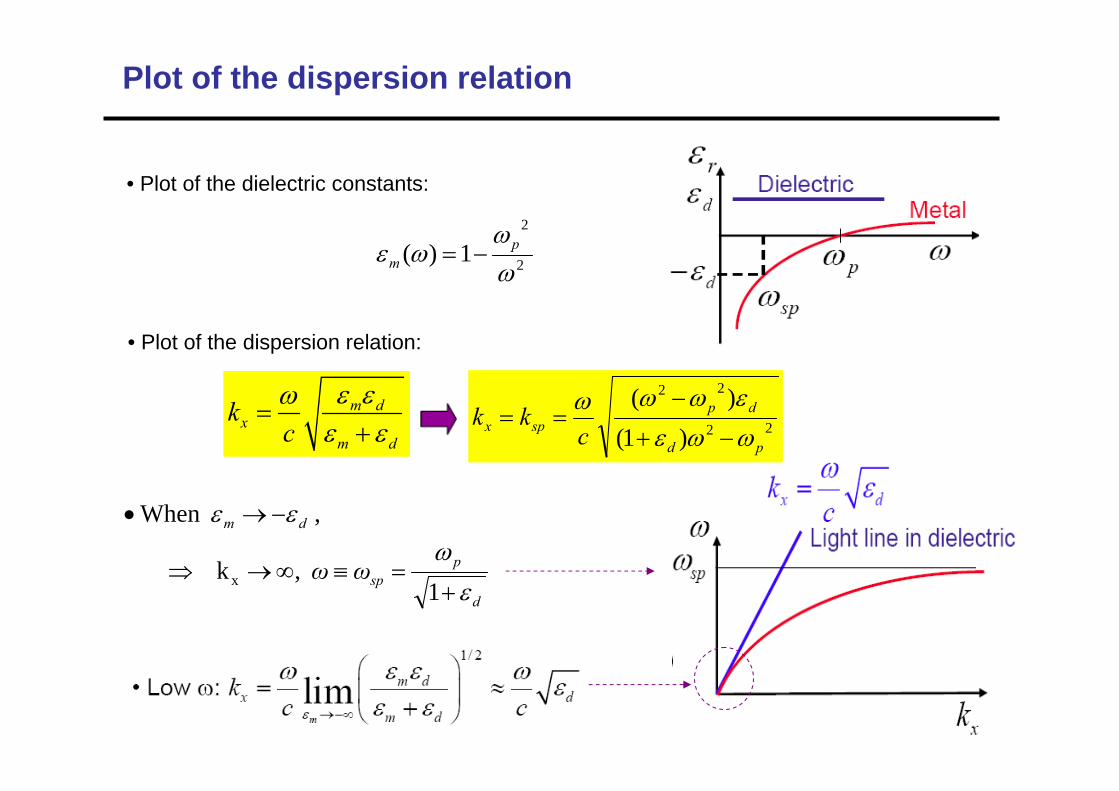
Plot of the dispersion relation

2

2

1)(ωω

ωε pm −=

m dx

m d

kc

ε εωε ε

=+

• Plot of the dielectric constants:

• Plot of the dispersion relation:

d

psp

dm

ωωε

ωεε

+=≡∞→⇒

−→•

1 ,k

, When

x

22

22

)1()(

pd

dpspx c

kkωωεεωωω

−+

−==

Surface plasmon dispersion relation:

2/1

⎟⎟⎠

⎞⎜⎜⎝

⎛+

=dm

dmx c

kεεεεω

ω

ωp

d

p

ε

ω

+1

Re kx

real kxreal kz

imaginary kxreal kz

real kximaginary kz

d

xckε

Bound modes

Radiative modes

Quasi-bound modes

Dielectric: εd

Metal: εm = εm' +

εm"

xz

(ε'm > 0)

(−εd < ε'm < 0)

(ε'm < −εd)

2 2 2 2p xc kω ω= +

Surface plasmon dispersion relation 1/ 22

izi

m d

kc

εωε ε

⎛ ⎞= ⎜ ⎟+⎝ ⎠