94

‘Driving’ IS projects Marta Fernández-Diego and Julián Marcelo-Cocho Departamento de Organización de Empresas Universidad Politécnica de Valencia, ES Abstract Using a didactical car-driving metaphor, this paper deals with a proactive way of ‘driving’ projects with high uncertainty. The centrality of problem complexity and problem uncertainty are demonstrated, the mapping of these to human cognition is reviewed, and the car-driving metaphor as ‘driving’ project management is developed. The MadPRYX ‘suite’ develops didactic car-driving models and practical scoreboard metrics, looking for successful equilibrium of effectiveness-efficiency, conditioned by the levels and types of complexity and uncertainty in the project process and its environment Keywords: Complexity, Effectiveness, Efficiency, Evolution, Project Management, Risk, Success, Uncertainty. 1. Complexity and Uncertainty in projects Complexity X and uncertainty Y are mega-factors, threats and contributors to project risk (risk of no meeting the project objectives and results). Indeed, they are essential characteristics of any project and their consideration is a necessary step for any decisive advance in a taxonomy, causality, and resolution of risk, the same as in other relevant managerial duties (Fernandez 2008). Furthermore, complexity X and uncertainty Y can be shown to be not only necessary but sufficient for

describing the risk of a project situation and its evolution within its environment (see Appendix). The proof begins by clarifying the underlying reasoning of important papers about project risk management based on ambiguous or fuzzy meanings of X and Y.9 Next, this paper contributes mainly to build some Advances in IS Project Management Research, Education, and Practice, showing didactic Models of Project Driving (Marcelo 1999), and the practical MadPRYX ‘suite’ of Methods for Adapting and Driving Projects by their Risks, Uncertainty Y, and Complexity X (Marcelo 2007).

Finally, the proof of sufficiency opens the use of both X and Y for an efficient generalization of the project concept in all sectors that currently study the theory of complexity (Wagensberg 1994) in the perspective of a theory of mega-complexity (combining the project complexity and the uncertainty born in its environment).

2. ‘Planning on the Left Side and Managing on the Right’

This classical figure of the brain (Mintzberg 1976) is based on the Hall Project Management Risk Model (Hall 1998).10 The Hall model, linking basic organizational and intellectual functions located in specific areas of the brain,

9 The INSEAD model (De Meyer 2002a 2002b) e.g. assumes X and Y being necessary but non sufficient conditions, since it shows two other risk mega-factors, ambiguity and chaos. But other well-known authors (Klir 1988) believe that ambiguity and chaos are only two types of uncertainty. 10 The use of brain maps for describing managerial functions has influential followers such as (Herrmann 1990) or (Webster 1999). In this paper, these maps have only been metaphorically taken, after confirmation of the level of support for the affirmations made by Hall by well known science publishers such as (Carter 1998). The quadrants indicate only complimentary functional areas in a brain totally interconnected, rather than tendencies or inclinations of any type.

95

covers six disciplines, Plan, Produce, Measure, iMprove, Discover , and Design (PPMMDD), installed in the four brain quadrants, covering dynamic/static and long-term/short-term functions and knowledge (see figure 1):11

FRONTALRIGHT BRAIN

dynamic

static

Oppor-tunity

Plan

State

Impact

Metrics

Objectives

Imaginaciónfuturo

IMprove Measure

Plan Produce

DiscoverDesignIMAGINEFUTURE

KNOWNLOGIC

UNKNOWNEMOTION

MEMORYPAST

Countermeasures

A

C D

FRONTALLEFT BRAIN

OCCIPITALRIGHT BRAIN

dynamic

static

OCCIPITALLEFT BRAIN

B

long term short term

Risk

Variance

long term short term

Fig. 1. Cerebral map showing 6 disciplines and 4 ’circuits’ (source: own development).

A. The frontal left brain quadrant A holds the logic of known, with influence on the ‘circuit’ PPM (Plan-Produce-Measure) which collects facts; analyses results; resolves problems in the short-term; reasons with the facts; understands the situation; and emphasizes the differences with respect to the plan.

B. The occipital left brain quadrant B holds the memory of the past, with influence on the ‘circuit’ MMP (Measure-iMprove-Plan) which offers a long-term perspective to foresee prospects in a consistent and programmed manner.

C. The occipital right brain quadrant C supports imagination of the future, with influence on the ‘circuit’ DDP (Discover-Design-Plan) which provides long-term perspective on the circumstances; capitalizes on opportunities and develops a prospective vision based on own discovery.

D. The frontal right brain quadrant D holds a sense of emotion regarding the unknown, with influence on the ‘circuit’ PPD (Plan-Produce-Discover) which provides a short-term perspective regarding parts of the plan and production to be investigated; explores the requirements or technologies and its possible impacts on the plan; resolves problems intuitively; observes signs of imminent change; tolerates ambiguity; integrates ideas; and defies established policy.

3. Strategy for driving projects by their risks

The ‘Project Driving’ concept (including Planning and Monitoring during Execution) goes a step further than the brain metaphor, using motor-racing metaphors when discussing the execution of project guidance: projects are vehicles, their development environment is a racing circuit, and project managers are drivers. x In ‘formula races’ we use delicate and complex machines with sophisticated features on specially

prepared circuits with predictable risks (including perhaps a ‘killer curve’). x In ‘rallies’ we use robust vehicles on approximate and uncertain routes, with the boulevard and the

crude animal path serving as road (such as the ‘Paris-Dakar’) full of predictable and unpredictable risks.

11 These four brain quadrants correspond to the four gnostic, temperamental and organizational ‘circuits’ MMP-PPM-PPD-DDP, related in this case to the driving of projects.

96

3.1. ‘Formula’ strategic model for driving projects

A single driver-manager can handle a highly complex project – providing the circuit only contains predictable variations (curves more or less risky), and providing that the environment does not contain unpredictable uncertainties (metaphorically, the circuit must be surrounded by an insurmountable crash barrier). Although the driver uses all of his or her mental capabilities, he is basically using short-term frontal

functions; whether to remember with the left hemisphere the logic of a ‘known circuit’; or to anticipate an unknown factor in the curve ahead using the right hemisphere and adapt driving to the circuit (the predictable reference that structures the whole project). In this way he can focus all his attention on indicators of the vehicle’s behaviour to guarantee the ‘success’ of the project (with policies and contingency plans to respond to predictable, but resolvable risk events such as breakdowns, punctures, fire, etc.).

3.2. ‘Rally’ strategic model for driving projects

Rally-style driving takes place on highly uncertain circuits and environments, with predictable and unpredictable risks, and requires two directors or at least, two functional directives (see figure 2).

(long-term) (short-term)

Improve

Plan

Discover

Produce

Design

Measure

Unknown

Emotion

LogicMemory

KnownPast

ImaginationFuture

(static)

(dynamic)

Fig. 2. ‘Rally’ driving, using both brain hemispheres (source: own development).

The co-driver monitors the circuit and its environment by reading a map. He tells the driver about the known risks on the circuit (predictable uncertainties) having acquired this information before the race as part of the planning process. In this way, he uses the functions of ‘memory of the past’ and ‘logic of known’ found in the left hemisphere of the brain.

The driver incorporates as ‘imagination of the future’ the preventive indications of the co-driver (predictable uncertainties); and performs the long-term manoeuvres (gear and speed changes). However, the driver uses the right cerebral hemisphere capabilities to handle the unknown (unpredictable uncertainties) that may arise, reacting with the brake and steering wheel.

Rally-style driving is best used in projects with great uncertainty, where the correlation of the functions of the driver and co-driver and the functions of both hemispheres are reflected and handled –

97

according to the resources and capabilities available - by a team of specialist managers; or by a single manager with an uncommon ability to realize both functions, but capable of differentiating and combining the roles of driver and co-driver.

4. Proactive project driving

When confronted by risk from an incident generated by environmental uncertainty (a ‘Murphy’), buffers of resources reserved for these risk situations allow the driver to continue. However, driving ‘by sight’ alone supposes not only a reactive step with respect to the project’s environment, but a proactive step with respect to the project itself;; learning to use a ‘map’ (project plan) when analyzing a situation, while resolving small and immediate incidents mechanically. The planning function, in a situation of high uncertainty Y, is converted in a sense into a series of

‘mappings’ that; firstly, shortens the trip to the immediate ‘journey’ ahead with a certain and precise objective (meaning a sub-project or prototype, hereby baptised ‘protoject’); and secondly, virtually achieves the objective and so places the ‘protoject’ in the context of the project. The breakdown of the project in tasks changes, to becoming a set of iterations, or ‘protojects’, that are structured according to the most convenient segments and milestones from the point of view of the resolution of uncertainties (that is, predictable incidents). The ‘danger map’ establishes the most dangerous areas and the most adequate driving measures (for example, speed limits, extra resources to climb ‘hills’, environmental attention frequency, reviews, etc.).

The monitoring function is based on a comparison between what is indicated on the ‘danger map’ (performed by the co-driver function or something like an audio GPS system), and what is ‘in sight’ in each planned interval of the ‘protoject’. This comparison requires the availability of a set of parameter measurers and measurement activators properly interrelated as a Balanced Scorecard; as well as interconnected between them (with measurement and action parameters adjustable as the project advances, in a similar way to automatic transmission or ‘softness’ of the suspension).

The ‘by sight driver’ must maintain global awareness of the project, as well as paying precise attention to the instruments and course, as suggested in the Theory of Constraints underlying the Critical Chain Project Management. The progressive depletion of the ‘major resource reserve’ (energy in the case of a vehicle) maintains a good level of efficiency in the project; while the ‘small reserves’ (including the activator’s space-time margins) enable rapid rectifications required by the relevant contingencies.

5. Risk Management and Project Success Factors

The study of Critical Risk Factors of a project parallels the study of its Critical Success Factors, taken as a result of fulfilling the objective in a way that can be factorized and measured with two criteria:

x Effectiveness is an ‘external’ criterion of result comparison with the objective established outside of the development of the project; a qualitative criterion (client satisfaction, for example) that implies sub-criteria which are difficult to validate and rarely validated.

x Efficiency is an ‘internal’ criterion of result comparison with some reference related to the limitation of resources used in the project, or with the causes of its potential defects. Its measurement is quantitative or qualitative, and more or less subjective; but it can be referenced to the degree of advancement achieved by the project, which can, in turn, be determined by material and immaterial resources used by the participants.

98

These two criteria are not independent, but rather di-synergic or negatively synergic. Efficiency is more controllable, but impacts effectiveness when certain resources are unavailable. Strategic ineffectiveness (abortive shortages) conditions the interest of any tactic efficiency. Even in well organized projects without abortive shortages, a risk of minor non-fulfilment may produce an impact that always requires an increase in resources (meaning a controlled reduction in global efficiency) in order to redirect the project towards the objective.

In general, to achieve a certain level of effectiveness (or a threshold of risk represented by a limited distance between the result and objective), the level of efficiency, or used resource, depends on the levels of uncertainty Y in the development process, until the maximum level of inefficiency implied in abandoning of the project. Before arriving at such an unsatisfactory decision, the lowest possible consumption of resources will minimize waste and reduce inefficiency.

6. Basic characteristics of the MadPRYX method

The MadPRYX method collects the two project guidance strategies of ‘formula’ and ‘rally’ – and works by means of functions included in every project management, represented as a sequence of stages, as in PMBoK (ANSI 2004):

x Initiating function includes search and selection of all the possible information about the project and its environment and establishes an external objective for the project; assuring its viability (in clarity, scope, and resources).

x Planning function proactively prepares contingency plans and safeguard policies to prevent predictable risks, and responds to the appearance with necessary resources (including buffers).

x Monitoring (of production) function reacts to alerts (established in previous functions) with planned countermeasures (the policies deduced in the contingency plans for predictable uncertainties), and responds to the appearance of these risks with generic resources (buffers and others); and resolves unpredictable uncertainty. This function has the necessary flexibility to respond to unpredictable errors using adaptive buffers such as learning.

x Executing function includes the tasks reserved for the project manager – handled in parallel with his task of monitoring the production team operations.

x Closing function gathers experiences and project metrics to prepare for the application of new parameters to successive projects - as learning for predictable risks.

During the executing and monitoring stages, given the constructive necessities of the content of the project, the previously listed functions can, in the case of a high complexity X, be reiterated with respect to the itemised modules or the prototypes designed to reduce the high level of uncertainty Y.

7. Conclusion

This paper deals with a proactive way of ‘driving’ projects with high uncertainty, providing increased control by deviating from the reference (i.e., moving from a previous plan to one more adaptable to the evolving situation). The MadPRYX ‘suite’ develops didactic car-driving models and practical scoreboard metrics, looking for successful equilibrium of effectiveness-efficiency, conditioned by the levels and types of complexity X and uncertainty Y in the project process and its environment.

A second perspective deals with ‘natural’ systems evolution (that is, projects ‘driven’ by their environment, with high uncertainty Y due to weakness or lack of internal objectives): the system S evolves looking for its minor dependency of environment E for avoiding danger to the complexity X of system S by a 'catastrophic’ deviation of the uncertainty Y due to environment E (not isolating

99

system S, but increasing its capacity to anticipate and/or reducing the system S impact on its environment E).

Appendix A. Sufficiency of Complexity and Uncertainty as Project Management risk factors

Risk - defined as a variable related with change - in any project (seen as a dynamic system S interfacing with its environment E) needs two and only two mega-factors, the complexity X of S and the uncertainty Y linked to relations between S and E. The proof will rely on two considerations: 1) The characterization of both factors X and Y by two shapes of the same entropic variable in the two

complementary sets S and E, embraceable by only one global entropic variable in the union ES of both sets, gathering both factors as instances of a mega-complexity Z.

2) The exhaustive ecosystem ES of the ‘universe’ embraced by S and its E. That property is needed only for the boundary relations between S and E, where the ‘distance’ to the boundary would weaken, like in the gravitational models.

A.1 Complexity, uncertainty, entropy and information

The proof starts from the Shannon axiom about the conceptual identification between uncertainty and a kind of entropy, in order to extend this axiom to a new analogy between the complexity of the system and another type of entropy. If p(i) in the Shannon formula measures the probability that an individual belongs to the species i, the System Entropy or ‘diversity’ AI (the amount of average information of S) provides a measurement of its complexity. We can define both concepts of System Complexity X and Environment Uncertainty Y based on two different kinds of the same entropy; with S and E considered separately; or altogether, based on a combined entropy of the combined ecosystem ES of S and E.

In order to coordinate these three entropies, the Information Theory can be applied to ecosystem ES in its part referred to the source, alternatively or jointly with Systems Theory, reconstructing all the Shannon arguments on this combination of Information and Systems Theories. The ‘ecomatic’ model starts therefore from a structure of three sets (E, S, ES) with the three types of entropy that measure the different amounts of structural information needed to describe the system E, its environment S and the relation between both. The omission of any evolution parameter, like time t, does not imply that the situation can not be modified, but only that the regime is considered stationary or non transitory: 1) The complexity X of system S is the entropy H of the structure (of states si) of S and measures in which degree

its alternatives can be reached:

),p(sS

n;logX[S]);p(slog)p(s-H[S]X[S]

i

2i2n i

d ¦ (1)

where S is the set of probabilities of the n states si of S. 2) The uncertainty Y of environment E is the entropy H of the structure (of states ei) of E and measures in which

degree its alternatives can be reached:

),p(eE

m;logY[E]);p(elog)p(e-H[E]Y[E]

j

2j2m j

d ¦ (2)

where E is the set of probabilities of the m states ej of E. 3) The average entropy H[S/E] of system S for a ‘standard’ state of environment E connects complexity and

uncertainty in the ecosystem ES:

)/ep(slog)/e)p(sp(e-

eS)p(eH[S/E]

ji2m n jij

jm j

¦ ¦¦

@ (>+ (3)

4) The transmission T[S,E] between S and E is the average amount of information trans-bordered, H[S] exits from

100

S, but H[S/E] will not arrive to E: S]T[E,H[E/S]-H[E]H[S/E]-H[S]E]T[S, (4)

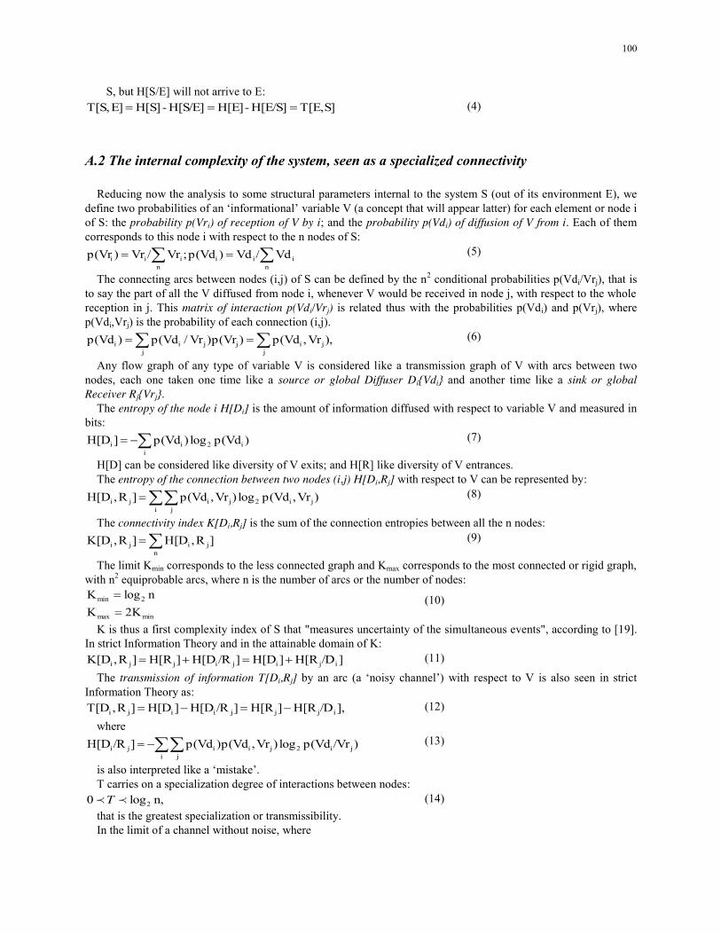
A.2 The internal complexity of the system, seen as a specialized connectivity

Reducing now the analysis to some structural parameters internal to the system S (out of its environment E), we define two probabilities of an ‘informational’ variable V (a concept that will appear latter) for each element or node i of S: the probability p(Vri) of reception of V by i; and the probability p(Vdi) of diffusion of V from i. Each of them corresponds to this node i with respect to the n nodes of S:

¦¦ n

iiin

iii Vd/Vd)p(Vd;Vr/Vr)p(Vr (5)

The connecting arcs between nodes (i,j) of S can be defined by the n2 conditional probabilities p(Vdi/Vrj), that is to say the part of all the V diffused from node i, whenever V would be received in node j, with respect to the whole reception in j. This matrix of interaction p(Vdi/Vrj) is related thus with the probabilities p(Vdi) and p(Vrj), where p(Vdi,Vrj) is the probability of each connection (i,j).

¦¦ j

jij

jjii ,)Vr,p(Vd)p(Vr)Vr/p(Vd)p(Vd (6)

Any flow graph of any type of variable V is considered like a transmission graph of V with arcs between two nodes, each one taken one time like a source or global Diffuser DiVdi and another time like a sink or global Receiver RjVrj.

The entropy of the node i H[Di] is the amount of information diffused with respect to variable V and measured in bits:

¦ i

i2ii )p(Vdlog)p(Vd]H[D (7)

H[D] can be considered like diversity of V exits; and H[R] like diversity of V entrances. The entropy of the connection between two nodes (i,j) H[Di,Rj] with respect to V can be represented by:

¦¦ i j

ji2jiji )Vr,p(Vdlog)Vr,p(Vd]R,H[D (8)

The connectivity index K[Di,Rj] is the sum of the connection entropies between all the n nodes:

¦ n

jiji ]R,H[D]R,K[D (9)

The limit Kmin corresponds to the less connected graph and Kmax corresponds to the most connected or rigid graph, with n2 equiprobable arcs, where n is the number of arcs or the number of nodes:

minmax

2min

K2KnlogK

(10)

K is thus a first complexity index of S that "measures uncertainty of the simultaneous events", according to [19]. In strict Information Theory and in the attainable domain of K:

]/DH[R]H[D]/RH[D]H[R]R,K[D ijijijji (11)

The transmission of information T[Di,Rj] by an arc (a ‘noisy channel’) with respect to V is also seen in strict Information Theory as:

],/DH[R]H[R]/RH[D]H[D]R,T[D ijjjiiji (12)

where

¦¦ i j

ji2jiiji )/Vrp(Vdlog)Vr,p(Vd)p(Vd]/RH[D (13)

is also interpreted like a ‘mistake’. T carries on a specialization degree of interactions between nodes:

n,log0 2%%T (14) that is the greatest specialization or transmissibility. In the limit of a channel without noise, where

101

,p)/Vrp(Vd ijji (15)

the ‘mistake’ disappears; or it equals the value H of the source of information if the transmission is lost in the channel:

)p(Vd)/Vrp(Vd iji (16)

The global ‘mini-complexity’ of system S is a type of internal complexity resumed as the duple <K,T> of connectivity K and specialization T of the S graph. K and T are associated in several ways, as Venn diagram shows easily (see figure 3).

K(Di,Rj)H(Di)

H(Di/Rj) T(Di,Rj)

H(Rj)

H(Rj/Di)

Fig. 3 Venn diagram for mini-complexity of system S (source: own development).

Thus:

],/RH[D]/DH[R]R,T[D]R,K[Dnlog2]H[R]H[D]R,T[D]R,K[D

jiijjiji

2jijiji

d (17)

TKthen ;0T-K As (18)

A.3. Interaction between the system S and its environment E

The partition of S into n components (or nodes) is initially arbitrary; but once conceived or made, the structural probabilities p(Vdi/Vrj),p(Vrj) remain completely defined. The real problem will only require adding some restrictions (inequations). E.g. we obtain stationary states related to activity V if the V flow disappears in each node of the graph (the node neither gains nor loses V); that is:

n ..., 1,i allfor )p(Vr)p(Vd ii (19) All this can now be applied if the ecosystem ES is considered like an isolated system, taking the environment E

like a node, node ‘0’. The uncertainty Y of E relating E (now node ‘0’) to the other nodes of S can be considered in this case as a special type of complexity (or relation <K,T> between nodes) included in a ‘mega-complexity’ Z of ES seen as an isolated system (see figure 4).

Ecosystem ES

EnvironmentE System S

External Entity

Node ’0’ Node 2

Node 3

Node 1

Vd2Vd3

Vd1

1Vr1

Vd0

Vr0

Vr2

Vr3

Fig. 4 Dual view of S+E or ES (source: own development).

Coming back to the modification scheme M of the ecosystem ES as the set of probabilities p(si/ej) and taking now the set of states of (E,S) as the variable V:

Z[M]H[M])/ep(slog)e,p(sE]K[S,H[S/E]H[E]S]K[E,

n mji2ji

¦¦ (20)

that is to say the ‘mega-complexity’ Z of the ecosystem ES. The matrix of conditional probabilities p(si/ej) resumes the interaction between S and E, transmitted by a ‘noisy

virtual channel’ acting as intermediate between two extreme values:

102

1) A ‘permeable channel’ where: H[S];T[S/E]0H[S/E] (21)

that is: ji if 1)/ep(sj;i if 0)/ep(s jiji % (22)

2) A ‘non permeable channel’ where: 0;T[S/E]H[S]H[S/E] (23)

that is: )p(s)/ep(s iji (24)

The conditional probability p(si/ej) means the probability that ‘informational variable’ si is seen in system S whenever environment E emits an ‘activity’ ej; that is to say the capacity of system S to perceive what happens in its environment E and the capacity to answer to the state of E.

A.4 ‘Ecosistemics’, evolution, adaptation and survival

Each type of System S (with its partition in an internal graph and related to its environment E) has some channel 'permeability' for each type of 'informational variable' V. The more interesting V is the 'auto-conscience’ of the system S, that is to say the information about its own mini-complexity X or about its mega-complexity Z –if it includes uncertainty and its relations with its environment E.12 The 'adaptive’ criterion is the core of the Evolution Theory of complex systems established experimentally

with biological populations of ecosystems ES. In these ecosystems, some characteristics constitute tactics of 'differentiability', like camouflage into environment E (a prey changing to non attractive colors to survive) or detaching out of E (a male changing to attractive colors to reproduce).

References

ANSI (2004) A Guide to the Project Management Body of Knowledge, PMBoK. PMI Carter R (1998) Mapping the Mind. The Orion Publishing Group Ltd. De Meyer A, Loch C, Pich M (2002 a) On Uncertainty, Ambiguity and Complexity in Project Management. INSEAD De Meyer A, Loch C, Pich M (2002 b) Managing Project Uncertainty: From Variation to Chaos. MIT Sloan Management Review Fernandez M, Marcelo J (2008) Project management, Complexity & Uncertainty. WCC Hall E (1998) Managing Risk. Methods for Software Systems Development. Software Engineering Series, Addison-Wesley Longman Herrmann N (1990) The Creative Brain. Brain Books Klir G, Folger T (1988) Fuzzy sets, uncertainty and information. Prentice Hall Marcelo J (2001) From Managing Risks in Projects to Managing Projects by their Risks [(RM PM) (PM RM)]. Tutorial imparted

at QUATIC 2001, 4th Encuentro para la Calidad en las TIC, Instituto Superior Técnico, Lisbon Marcelo J (2004) Risk in Systems and Projects with High Complexity and/or Uncertainty. Ph.D. dissertation. Universidad Politécnica de

Valencia Marcelo J (2007) Driving projects by their risks. Upgrade. CEPIS. http://www.upgrade-cepis.org/issues/2007/5/upgrade-vol-VIII-5.html.

Accessed 1 December 2007 Mintzberg H (1976) Planning on the Left Side and Managing on the Right. Harvard Business Review, July-August, p. 49 Wagensberg J (1994) Ideas about the complexity of the world. Tusquets Editores, Spain Webster G (1999) Managing Projects at Work. ISBN 0 566 07982 8

12 The accepted additivity of the different entropies and other dimensionally similar operands follows the traditional Boltzmann-Gibbs formulation of energy and entropy. The needed generalization of this formulation can be seen in C. Tsallis and E. Cured, “Generalized statistical mechanics: Connections with thermodynamics”, Journal of Physics, 1991.