Embed Size (px)
Citation preview
DRIVER POPULATION FACTORS
IN FREEWAY CAPACITY
Submitted to: Florida Department of Transportation
Center for Urban Transportation Research College of Engineering, University of South Florida
4202 E. Fowler Avenue, CUT 100 Tampa, Florida 33620-5675
Principal Authors:
J. John Lu, Ph.D., P.E. Weimin Huang
Edward A. Mierzejewski, Ph.D., P.E.
May 1997

Tf.OCNlCAL R.UORT DOCUME."'lTA1'10N PACt
I. fttpottHo. 1. ~Mention No. (NTIS) 3. R~IC~NCI.
WPI No. 0510759
4. T~WS!Itllilla $. R•POn D•c• Driver Population Factors In Freeway Capacity 5197
6. I'Wfoml~ ~Cion. Cedi
7. NJtllot'(.) a. Pcdormifle ~R.pon No.
J. John Lu. Ph.D., P.E .. Weimin Huang, and Edward A. Mierzejewski, Ph.D .. P. E. . t . P~~O~Nwn•.c!Ackh» 10 . v.b'klkllHo. (TRAJ$)
Center for Urban Transportation Research USF College of Engineering
11. COI'IW'td « Grvt No. 4202 E. Fowler Avenue. CUT 100 Tampa, FL 33620·5675 6·9875
11. spomomg ..aqoncy N...,.,• Olld Acli:hn 13. Typo of Rtp0tt Olld Ptriocl C:O¥w.cl
FOOT Department of Transportation Final Report 605 Suwannee Street 8/14195 . 5130/97 Tallahassee, FL 32399-0450
. t4, $potl101'1r1Q A9MCY Codl
1!1, ~*"'tntwy HotM
16. Ab.ncl
The methods contained in the Highway Capacity Manual are based on a traffic composition of local drivers familiar w~h roadway characteristics. The Manual allows for the incorporation of a driver population factor adjustment into freeway capacity calculations to reflect the influence of unfamiliar drivers. Unfortunately, the Manual offers very little guidance on the appropriate values of the factor.
This project used continuous count traffic data at a number of Florida freeway locations to estimate the appropriate values of the driver population factor. By relating speed-volume characteristics to measures of non~ocal driver populations, the importance of this factor was demonstrated. Estimates were made of the factor values based on a sample of locations in Florida.
l ' 17. l(eyW«ds 11. Ois".ritlutiM &.t~•mtnt i highway capacity, driver Report available to the public through the
characteristics. tourist travel National Technical Information Service (NTIS) I 5285 Port Royal Road • Springfield, Virginia 22161 '
(703) 487-4650 1&. s.o.,.rii)'C .. t.W.(ei'INt~ 20. Soo..rittCIM_,,(otthi•~l 21. No. of poget. .......
j unclassified unclassified
Form DOT F 1700.1 (8-72) Rt.prochtttion ot wmplettd page au1horiztd

DISCLAIMER
The opinions, findings, and conclusions expressed in this interim technical report are
those of the authors and not necessarily those of the State of Florida Department of
Transportation.
iii

ACKNOWLEDGMENTS
The authors express their sincere apprec1alion to the Florida Department of
Transportation for its support of this project. In particular, the assistance of the following
individuals is recognized: Douglas McLeod and Kurt Eichin of the Systems Planning
Office, Harshad Desai and Rick Reel of the Transportation Statistics Office, and Richard
Long of the Research Office. It was through their support and assistance that this project
became a reality.
iv

TABLE OF CONTENTS
LIST OF TABLES ................................................................................................................. vii LIST OF FIGURES ..................................... -.................................................................... viii
CHAPTER 1: .................... ......................................................................... ............................... ! Background ............... .......................... .................................................................... .......... I Research Problem Statement ..... ....................... ...... ........... ...... ... ............ .......................... 5 Study Performed ............................................................................ .......... ...... ................ ... 6 Scope of the Report .................................................................................... ...................... ?
CHAYI'ER 2: REVIEW OF PAST STUDIES ................................................................ 9 Capacity Analysis and the Highway Capacity Manual ........... ......................................... 9 Reviews of fw and t;w Adjustment Factors .......................................................... ....... .... ! 0 Past Studies of Driver Population Factors ...... .............. ... ............................................... 12 Other Related Studies ... ... ........... ... ................................................................................ . 15
CHAPTER 3 : PRINCIPLE USED IN THE PROJECT ............................................ 16 Definition of Non-Local Drivers .................... ... .............. ... ...... ... ... ... ............ ................. 16 Basic Concept ...... ... ...... ... ........... ... ... ............................................. ............................. ... . 16 Estimation of Non-Local Driver Population Levels ...................................................... .!? Principle ... ......... ...... ......... ... ... ....................................... .................................................. l8 Calibration of Population Adjustment Factors .. ........... ... ............................................... 22
CHAPTER 4: RESEARCH DATA SOURCE$ ........................................................... 24 Traffic Data ....... ............... .................................................................... ....................... .... 24 Tourist Survey ............................................................................................... ... .............. 26 Estimation of Non-Local Driver Population Levels Using Tourist Survey Data ........... 27 Estimation ofNon-Local Driver Population Levels Using Traffic Data ........................ 30
CHAPTER 5: DEVELOPMENT OF DRIVER POPULATION ADJUSTMENT FACTOR TABLE BASED ON TOURIST SURVEY DATA ...................................... 37
Modeling Procedure and Results .......... ................. ........... ... ......... ..................... ... ...... .... 37 More Generalized Results ............................................................. .................. ............ .... 45 Estimate of Driver Population Factors Based on Test Site 0130 .................................. 46 Discussion ........................................................................................ .............................. .4 7
CHAPTER 6: DEVELOPMENT OF A DRIVER POPULATION ADJUSTMENT FACTOR TABLE BASED ON TRAFFIC CHARACTERISTICS ............................ 49
Monthly Factors, Weekly Factors, and Daily Factors ..................................... ...... ........ .49 Monthly factor ........................................................... .......................... ........................ 49 Weekly factor .... ... ... ... ................................................... ... ... ... ..... ...... ............. ... .......... . 5! Daily factor .. , ................... ......... ......................... ........ ...... ........................................... . 52
v

TABLE OF CONTENTS (CONTINUED)
Correlation between monthly factor, weekly factor, and daily factor .............. ........... 53 Speed-Volume Models ....... , .......................................................................... ................. 54 Development of an Index ......................... ... ........... ... ... ... ... ... ...... .................................... 57
Model Specifications ........... ...... ........... ................. ...................................................... 51 Index calibration .................. .................................. , ....... ................................ .............. 57 Final index ............................................ ....................................................................... 58
Impact ofNon-Local Driver Population Levels on Speed-Volume Curves ........ ........... 59 Estimate of Driver Population Factors .......................................................................... 60 D
. . JSCUSSJOn ....................................... ............................ .................................................... 63
CHAPTER 7: SUMMARY, CONCLUSIONS, AND RECOMMENDATIONS ...................................................................................... 64 s l1llll1l ary .................................................................................................................... ..... 64 Conclusions .................................... ...... .......................................................................... 65 Recommendations ..................................... .......................................... ... ... ... .................. 68
REFERENCES ...................... ... ,_ .............................................................................................. 69
vi

LIST OF TABLES
Table 1-1: Adjustment Factors for Driver Populations (HCM 1994) ................................ .4
Table 1-2: Annual Vehicle-Mile Traveled in USA and Florida ......................................... 5
Table 2-1: Reconunended Population Adjustment Factors by Sharma ........................... l4
Table 4-1: FOOT Traffic Count Stations and AADT ...................................................... 26
Table 4-2: TIVD and 01 Values for the Orlando Area ................................................... 29
Table 4-3: MF, WF, and OF Values ................................................................................ 34
Table S-1: Regression Analysis Results (a & bin Eq. 5-1) (1-4, WB, Orlando, Site: 0 130) and Monthly Non-Local Driver Indices (DI) (Orlando ) ................................. .40
Table S-2: Maximum Service Volumes (pcphpl) for LOS B, C, and D and Different DI Values .......................................................................... ...... ........................... .47
Table S-3: Driver Population Adjustment Factors for Different Levels of Service, Based on Orlando Conditions ............................................................................................ 48
Table 6-1: Correlations between Factors ..... ., .................................................................. 54
Table 6-2: Speed-Volume Models at the Three Sites ...................................................... 55
Table 6-3: Index Model Specifications ........................................................ ... ............ ..... 57
Table 6•4: Index Model Calibration Results .................................................................... 58
Table 6-S: Maximum Service Volumes (pcphpl) for LOS B, C, and D and Different NDI Values ................................................... ........... ... ......... ............ ................... 61
Table 6-6: Driver Population Adjustment Factors for Different Levels ofService ......... 62
vii
LIST OF FIGURES
Figure 1-1: Speed-Flow Characteristics for Basic Freeway Sections (For Ideal Conditions): (a) Four Lane Freeways, (b) Six-or-More-Lane Freeways. (HCM 1994) ................................................................... ........................ ........................... ... 2
Figure 3-1: Impact of Non-Local Driver Population .................. ...... .............. ................. 19
Figure 3-2: Typical Relationship between Volume and Speed (1-4 WB Middle Lane, March 1995, Orlando) .......... ... .................. .................................... 20
Figure 3-3: Concept of Estimating fp .......... .................................................................... 21
Figure 3-4: Basic Principle of Developing Driver Population Adjustment Factors ....... . 23
Figure 4-1: Locations ofFDOT Traffic Count Stations ................... ... ............................ 25
Figure 4-2: DI Values for Different Months in Orlando Area ................. ........................ 30
Figure 4-3: MF Values for Different Months in Orlando Area (WB and Lane I Only) .................................................................................................. ..... 32
Figure 4-4: WF Values for Different Months in Orlando Area (WB and Lane I Only) .................................................... ......... ...... ................................... .33
Figure 4-S: OF Values for Different Months in Orlando Area (\VB and Lane I Only) .... ........................................... ........................................................ 33
Figure 5-1: Relationship between Volume and Speed (I-4 WB Lane I, January 1995, Orlando, Site: 0130) ....................... ......................................................................... 38
Figure 5-2: Relationship between Volume and Speed (1-4 WB Lane 2, October 1995, Orlando, Site: 0130) .................................................................................. .......... .... 38
Figure 5-3: Relationship between Volume and Speed (1-4 WB Lane 3, March 1995, Orlando, Site: 0 130) ............. ... ........... ... ........................................... .......... .......... ... 39
Figure S-4: Statistical Relationship between Parameter "b" and Monthly Non-Local Driver Index (DI) (I-4 WB, Orlando, Site: 0130) ....................................... .... .41
Figure S-S: Statistical Relationship between the Average Value of Parameter "b" and Monthly Non-Local Driver Index (DI) (with 2"'-order polynomial curve) .............. .43
viii

LIST OF FIGURES (CONTINUED)
Figure 5-6: Impact of Non-Local Driver Population on Average Operating Speed (1-4 WB, Orlando, Site: 0130) ........... .............. ...... ................. ... ... ... ...... ....... ... ... ............ .44
Figure 5-7: Impact ofNon-Local Driver Population on Average Operating Speed (1-4 Both Directions, Orlando, Site: 0130) ..................... ................................................ .45
Figure S-8: Estimation of Driver Population Adjustment Factors (1-4 Both Directions, Orlando, Site: 0130) ...... ................................................................ 46
Figure 6-1: Monthly Factors of Different Months at Sites 0130, 0171, and 0174 .......... 51
Figure 6-2: Weekly Factors of Different Months at Sites 0130, 0171, and 0174 ...... ..... .52
Figure 6-3: Daily Factors of Different Months at Sites 0130, 0171, and 0174 ............... 53
Figure 6-4: Impact ofNon-local Driver Population on Average Operating Speed ......... 60
Figure 6-5: Density Line for LOS C (14.92 pclkmlln) ................ .................................... 61
ix

CHAPTER 1: INTRODUCTION
Background
The capacity of a roadway facility is defmed as the maximum number of vehicles that can
be accommodated by the facility during a given time period. Capacity analysis of
freeways is one of the important procedures, as freeways generally carry a high
proportion of an area's traffic. Freeway capacity analysis procedures have been used to
evaluate level of service (LOS) of basic freeway segments, design number of freeway
lanes, and estimate the maximum service flow at prevailing conditions.
The Highway Capacity Manual (HCM) published by Transportation Research Board has
been the guidance for capacity analyses since it was first published in 1950 (HCM 1994).
The latest version of the HCM is the 1994 Update of the Third Edition (HCM 1994). The
HCM covers every major aspect in highway transportation, including freeways, rural
highways, urban streets, transit, bicycles, and pedestrians. In the freeway section, the
HCM includes basic freeway segments, weaving areas, ramps, ramp junctions, and
freeway systems. The generalized analysis approach in the HCM consists of three major
steps. The first step is to find the capacity of highway facilities under ideal conditions.
Second, the levels of service are used to represent different operating qualities and to
determine the maximum flow rates under these different levels of service. Finally,
adjustment factors are applied to the ideal conditions to adjust capacity and the maximum
flow rates at different levels of service to take account of capacity reductions caused by
prevailing (non-ideal) roadway and traffic conditions.
In the HCM, speed-volume models are used for the capacity analysis of the basic freeway
segments under ideal traffic and roadway conditions. Different curves are provided for
four-lane freeways and six-or-more-lane freeways at different free flow speeds. Figure I
I presents the speed-flow curves copied from the 1994 HCM. The capacity under ideal
conditions is 2,200 passenger car per hour per lane (pcphpl) for four-lane freeways and
2,300 pcphpl for six-or-more-lane freeways (HCM 1994).

Figure 1-1: Speed-Flow Characteristics for Basic Freeway Sections (For Ideal Conditions): (a) Four Laue Freeways,
(b) Sil:-or-More-Laoe Freeways. ( HCM 1994)
-" .... ... . ....... ...... ..... .... ....... , .. : ... ..... . . ... .. . . . ........ .. . · .. ~:a ,_ WPM : . Ba ~ .«:, , , : !300 ~J"-pi, ~ - • . , . ~ .. .. : , . . , .: .• . .. : ..
- lu .. ._ : · · · i.a.:o oc~ .. .. :. :
~:lw.~ : .-l&O~~··: ::: : : .. 1 .. - : . . . . . : ~:: E.vJ .. .. ; . ... .; . .. . . :. . . : .. . . .: . . . . .; . .... ; .. . .. :. .. . . :..~,.:: . .: . . a4SJ, .... ~ .. .. : .. ... : .... ~- · · · ·: · · · ·· : .. .. ~ ... .. ; ..... ; .... . ~· · ·· ·i·· · · · ; .. ~ . . . : ~~, · - · · : · · · ·: · · · · · ~ ·· ·· : ·· · -~ ·· · · · · · ·· ·· :·· · · ·: · · · · · :· · ··· : · · · ·r· · · · :·· eu- . · · ~ · · · · ; ..... :. .. ; ..... ; . . . . . :, . . . . ; . . . . .;. . .. .. : . . ... ; .. . i ,"E:· · · ···· ... \ . . . . . ' . . -·. . OM- · ·· ·' · · · · ··· ·· · ·· : ... . ... .. . ... . : . . ..... . . ... .. ... . . . G:,I: .. ..••
I • • • • • • • • u C • c ' . . . . . . . . ~;,, .. . l:l"~ . . . .. . .. . ... . . . . . .. . : . . . . : · .... .. .. . . : . . . . ·: · . . . ·:· . ... : . . . ;;·I •· .. - ~. c.. : • • • • • , o !t . : u; ····I' · ·. · · : · · · · ·:· · · · · .· · · · ·: · · · · ·:· · · · ·:· · · · ~ · · ::!:! ' · · ·: · :'~ 1·· ·· : · · · · : ,., . ·' · · · · ·>· · · · ·· · · · ~ · · ·· ·: · · -:·· · ·· : · · · ~ · · ··:- · ~':J ~ : : : ~· ~ ..... .. . : .. .. : ... ...... .. : .. · .. :· .. .. : .. .. ·: · .. ·j·
I · ·. ... .. . :· ·· ··. ·· ·· · .· · · · :· ·· . • . . . . , . • , , , · • ··, · · · · .· •
.~· --~--~--~--~--~~---r--,---~--r-~----_J ... . .. IOU:. fLOW R.lT.E TOR 15-loiiNUTt PtRIOO (PCPHPL)
(a)
,....1S-' · · · · · · ··· · · · ·· . . . . . ...... .. . .. . . ; ... . . . · . . . .. : I £, ' 1.0 """ •• "'' ;.;. Per. \300 ,c:;l:pt . . \
i~--~~.~:~::..:·_---------------:-·~;~"",~:"':~~ .. ·1
EH~ . ~~~~ I' <( • · ·: ~ .... ,
e~- :. . . . . . , I "~- h I - : ~ .. - ~ .
- !;!• I -c )<•
Q loo !!--~ !~--~ ~!-~ ._ ·c. ~
I•
L o
u ' . ~~r e ·: ~.~ N O • .:
"-
. Ill •• - ' '' ••• ' ' ' ' - •• '''' •• ~'' ••
!O!A, : :. cw hi~ (Cii I ~-"'-INtJi! P~_lj;.O ] (?~GH?!.)
(b)
2

Six levels of service, from LOS A to LOS F, are defined for freeways. LOS A represents
the best operations quality and LOS F the worst. LOS E is the situation where traffic
demand just reaches maximum facility capacity. As the traffic demand continues to
increase beyond the capacity, the LOS will degrade into tbe stop-and-go forced flow
condition of LOS F. The maximum number of vehicles that could pass a freeway section
in a unit time under each LOS is called the maximum service flow rate for that LOS,
except LOS F at which traffic conditions are unstable.
According to the HCM, the capacity of a basic freeway segment is based on the ideal
capacity that could only be observed under ideal roadway and traffic conditions. The
ideal roadway and traffic conditions for basic freeway segments are described as follows
(HCM 1994):
• Good weather,
• Good pavement conditions,
• No incident affecting traffic flow,
• Level terrain,
• 12-ft minimum lane widths,
• 6-ft minimum lateral clearance between the edge of the travel lane and the
nearest roadside or median obstacle or objective influencing traffic behavior,
• All passenger cars in the traffic stream, and
• A driver population dominated by regular and familiar users of the facility.
Capacity reductions of a basic freeway segment would be observed under prevail.ing
traffic and roadway conditions. To calculate capacity reductions due to prevailing
conditions, three adjustment factors, namely adjustment factors for lane widths and lateral
clearances (fw), adjustment factors for heavy vehicles (fHV), and adjustment factors for
driver populations (t;,) should be applied. This approach is mathematically described by
the following equation:
(1-1)
3

where
SF; = service flow rate for LOS i under prevailing roadway and traffic conditions
for N Janes in one direction, vph,
c; =the ideal capacity, 2200 pcphpl for 4-lane freeways or 2300 pcpbpl for 6-lane
freeways,
(v/c}. =maximum volwnelcapacity ratio for LOS i,
N = nwnber of lanes in one direction of the freeway,
f w = factor to adjust for the effects of restricted Jane widths and lateral clearances,
fHV =factor to adjust for the effects of heavy vehicles on the traffic stream. and
~ = factor to adjust for the effects of recreational or unfamiliar driver populations.
Among these three adjustment factors, there are specific definitions and clearly defined
calculation procedures for fw and fHV in the HCM, but only a very simple table is
presented for fP, as shown in Table 1-1. As noted in the 1994 HCM, the driver population
adjustment factor is said to range from 0.75 to 0.99 and is to be applied when there are
significant percentages of non-commuters in the traffic stream. Unfortunately, the HCM
offers little guidance on how to select appropriate values for this factor. As a result, the
driver population adjustment factor is commonly ignored. Without clear instruction on
selection of the driver population factor, significant bias may be introduced in capacity
analysis, particularly, in an area such as Florida with a significant percentage of tourism
traffic volume or non-commuters. Non-local drivers or non-commuters in the traffic
Table 1.1: Adjustment Fadors for Driver Populations (HCM 1994).
Traffic Stream Types Population Adjustment Factors
Weekday Commuters 1.00
Recreational or Other 0.75 - 0.99
4

stream may cause capacity reductions in several ways, including perception-reaction
time, car-following behavior, lane change and gap acceptance behavior, and driving
speed. As the percentage of non-local drivers or non-commuters increases, these factors
combine to contribute to the expected reduction in freeway capacity.
Research Problem Statement
Although the mileage of Interstate, Turnpike, and other fully access-controlled
expressways was only 1.7% of the total highway system in Florida in 1994,24.8% of the
total annual vehicle-mile-traveled took place on freeways in that year (HPMS 1994). A
safe and efficient freeway system is vital for the economy of Florida To achieve this
goal, traffic engineers should have a practical tool to perfonn freeway capacity analyses.
For decades, that "tool" has been the HCM. Applying adjustment factors is a very
important procedure in the analytical approach of the HCM.
Without appropriate definitions and practical calibration methods, it is difficult to make
reasonable estimates oft;, from the range of 0.75-1.00 as it appears in the HCM. This
defect is especially obvious in Florida. Many freeways in Florida have good geometric
desigJI, level terrain, and nonnal percentages of heavy vehicles, as shown in Table 1-2
(FHWA 1994). Such characteristics may result in the adjustment factors (fw and fuv)
approaching 1.0. On the other hand, Florida has many tourist attractions
Table J-2: Annual Vehicle-Mile Traveled in USA and Florida.
Passenger Cars Single-Unit 2-Axle
Freeway Types Motorcycles Buses & Other 2-Axle 6-Tire or More & (%) (%) 4-Tire Vehicles Combination Trucks
(%) (%)
Rural Nationwide 0.6 0.3 80.5 18.6 Interstate Florida 0.5 0.7 80.5 18.3
Urban Nationwide 0.4 0.2 91.8 7.6 Interstate florida 0.4 0.6 91.5 7.5
5
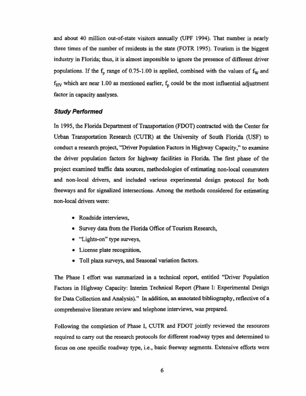
and about 40 million out-of-state visitors annually (UPF 1994). That number is nearly
three times of the number of residents in the State (FOTR 1995). Tourism is the biggest
industry in Florida; thus, it is almost impossible to ignore the presence of different driver
populations. If the fp range of 0.75-1.00 is applied, combined v.itb the values of fw and
fHV which are near 1.00 as mentioned earlier, t;, could be the most influential adjustment
factor in capacity analyses.
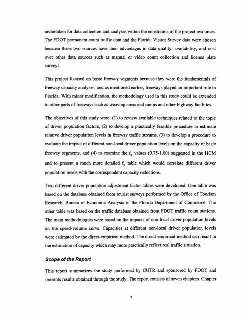
Study Performed
In 1995, the Florida Department of Transportation (FOOT) contracted with the Center for
Urban Transportation Research (CUTR) at the University of South Florida (USF) to
conduct a research project, "Driver Population Factors in Highway Capacity," to examine
the driver population factors for highway facilities in Florida. The first phase of the
project examined traffic data sources, methodologies of estimating non-local commuters
and non-local drivers, and included various experimental design protocol for both
freeways and for signalized intersections. Among the methods considered for estimating
non-local drivers were:
• Roadside interviews,
o Survey data from the Florida Office of Tourism Research,
o "Lights-on" type surveys,
o License plate recognition,
o Toll plaza surveys, and Seasonal variation factors.
The Phase I effort was summarized in a technical report, entitled ~Driver Population
Factors in Highway Capacity: Interim Technical Report (Phase 1: Experimental Design
for Data Collection and Analysis)." In addition, an annotated bibliography, reflective of a
comprehensive literature review and telephone interviews, was prepared.
Following the completion of Phase I, CUTR and FOOT jointly reviewed the resources
required to carry out the research protocols for different roadway types and determined to
focus on one specific roadway type, i.e., basic freeway segments. Extensive efforts were
6
undertaken for data collection and analyses within the constraints of the project resources.
The FOOT permanent count traffic data and the Florida Visitor Survey data were chosen
because these two sources have their advantages in data quality, availability, and cost
over other data sources such as manual or video count collection and license plate
surveys.
This project focused on basic freeway segments because they were the fundamentals of
freeway capacity analyses, and as mentioned earlier, freeways played an important role in
Florida. With minor modification, the methodology used in this study could be extended
to other parts of freeways such as weaving areas and ramps and other highway facilities.
The objectives of this study were: (I) to review available techniques related to the topic
of driver population factors, (2) to develop a practically feasible procedure to estimate
relative driver population levels in freeway traffic streams, (3) to develop a procedure to
evaluate the impact of different non-local driver population levels on the capacity of basic
freeway segments, and (4) to examine the fp values (0.75-1.00) suggested in the HCM
and to present a much more detailed fP table which would correlate different driver
population levels with the correspondent capacity reductions.
Two different driver population adjustment factor tables were developed. One table was
based on the database obtained from tourist surveys performed by the Office of Tourism
Research, Bureau of Economic Analysis of the Florida Depariment of Commerce. The
other table was based on the traffic database obtained from FOOT traffic count stations.
The main methodologies were based on the impacts of non-local driver population levels
on the speed-volume curve. Capacities at different non-local driver population levels
were estimated by the direct-empirical method. The direct-empirical method can result in
the estimation of capacity which may more practically reflect real traffic situation.
Scope of the Report
This report surnrnari2es the study performed by CUTR and sponsored by FOOT and
presents results obtained through the study. The report consists of seven chapters. Chapter
7

2 reviews past studies related to the topic of driver populations. Chapter 3 describes the
methodologies used in this project. Chapter 4 discusses the data resources used in the
project. Chapters 5 and 6 summarize the procedures developed through this study to
evaluate the impacts of non-local driver population levels on capacity reductions.
Chapters 5 and 6 present two different driver population adjustment tables obtained from
the study and based on the data collected in the study. The results shown in Chapter 5
were based on the tourist survey database, and the results shown in Chapter 6 were based
on the FDOT traffic count station database. Chapter 7 discusses conclusions, summaries,
and recommendations resulting from the srudy.
8
CHAPTER 2: REVlEW OF PAST STUDIES
Capacity Analysis and the Highway Capacity Manual
The earliest highway capacity studies dated back to the early 1920s when a capacity
analysis conunittee was set up by the Highway Research Board. In I 950, the first
Highway Capacity Manual was published by the Highway Research Board, and it quickly
became the standard for highway capacity analyses in the United States and many other
countries (HCM 1994).
In the 1960s, research attention was paid toward freeway capacity analyses along with the
construction of the Interstate Highway system throughout the nation (May 1990). In
1965, the second edition of HCM was published to replace the outdated I 950 HCM
(HCM 1994). The 1965 HCM included the level-of-service concept into the manual.
Since then, traffic has continued to grow at an even faster rate than new highway
construction, and as a result, traffic operations quality had become a major concern of
state and local transportation agencies and of the general public.
After rwo decades of comprehensive research, the third edition of HCM was published in
1985 by the Transportation Research Board. The 1985 HCM was viewed as a milestone
in the growing body of knowledge of highway capacity because of the extension into
facilities other than highways and the refinement on the LOS concept (HCM 1994). The
latest HCM is the I 994 Update of the third edition, marking another significant
achievement in highway capacity research (HCM 1994). In the freeway capacity analysis
sections of the 1994 HCM, fw and fHV tables were updated, and free flow speeds were
used instead of design speeds. The 1994 HCM included driver population factors for
freeways capacity analysis, but not for other facilities. It is possible that such factors
would be equally important for unintenupted flows on arterial as well as intersections.
The HCM covered every major aspects of highway transportation, including highways,
transit, pedestrians, and bicycles, and it plays an even more important role today because
9

transportation planners, designers, and operators are striving to maintain an efficient and
safe transportation system under more and more traffic demands and limited
infrastructure funding.
Reviews of fw and fHvAdjustment Factors
One of the most unarguable adjustment factors in the HCM is fw. and it has been in
practice for decades. Nowadays fw values are usually 1.00 in practice because new
highway construction normally has adequate lane widths and lateral clearances, and this
could also be the reason why very few recent reviews are available for fw studies
recently.
In the HCM, fHV is also a well developed adjustment factor with refined calibration
methods and detailed estimation. The most comprehensive ffiV study was documented in
a Federal Highway Administration report (FHW A 1982). Passenger Car Equivalents
(PCEs) were used to convert a traffic stream composed of a mixture of vehicle types into
an equivalent traffic stream composed exclusively of passenger cars. The fHV is computed
from such PCEs and the proportions of heavy vehicles in the traffic stream using the
following equation according to the HCM (HCM 1994):
where
(2-1)
E,., ~ = passenger car equivalent for trucks/buses and recreational vehicles,
respectively, and
P1, P, =proportion of trucks/buses and recreational vehicles respectively.
In this fHv study, vehicle classifications, headway, and speeds were collected in the field.
Then headway values of different vehicle types was compared with the standard headway
of passenger cars to determine the relative amounts of space coQSUmed by different
vehicle types. This approach is described by the following equation:
10

where
SH·· PCE, = ~
~ SHPCj (2-2)
PCEij =passenger car equivalent of vehicle type i in conditionj,
SHij = mean inter-vehicular spatial headway (measured from the vehicle type i's
rear bumper to the rear bumper of the leading vehicle) for conditionj, and
SHpq = mean inter-vehicular spatial headway (measured from a passenger car's
rear bumper to the rear bumper of the leading vehicle) for conditionj.
Another method used in the fHV study was to measure the equivalent delay. Drivers could
drive at any lawful speed except when they were obstructed by slower vehicles. PCEs
could be calculated from the different delay time of different vehicle types. This approach
is described by the following equation:
where
D,-Db PCE, = •J ase
~ Dbase
PCEij = passenger car equivalent of vehicle type i in condition j,
Dii = delay to passenger cars due to vehicle type i in condition j, and
Dbase = delay to standard passenger cars due to slower passenger cars.
(2-3)
These two methods are very effective for fHV estimation. Unfortunately, they are not
practical for ~ estimation due to the fact that it is much more difficult to determine the
driver type (driver population) than it is to determine the vehicle type. Manual surveys
and video taping could provide accurate information about vehicle type at a low cost and
sometimes even at a fast rate if image processing techniques are used. But these types of
observations offer little information about drivers. The license plate survey is not a
reliable source in detecting driver populations because this method could not identify
11

rental cars, most of which are driven by visitors. Rental cars could register in different
counties. It is also difficult to read customized license plates which are becoming more
and more popular in Florida. It is very difficult to record accurate driver information
without stopping traffic and doing conventional roadside interviews.
The conventional roadside interview is the only method to obtain direct information
about driver populations. This kind of survey is very costly, and in some locations such as
freeways, it is impractical to implement. The complexity and difficulty in driver
population estimation might be the reason why very limited research has been done.
Past Studies of Driver Population Factors
The Transportation Research Information Services (TRIS) is the Transportation Research
Board's bibliographic database; it is the most comprehensive and current source for
transportation information retrievals in the nation. The TRIS database contains document
abstracts describing the published literature of research on highway, transit, highway
safety, railroad, maritime and air transportation. In this study, the TRIS was searched to
find past studies related to driver populations. Only two articles were found from TRIS
with the topic keyword of"driver population factor." Both of the articles were written by
Sharma. One article (Sharma 1987) was based on his other article, "Road Classification
According to Driver Population" in the Transportation Research Record No. I 090
(Sharma 1986). The contents of his study will be discussed later in this section.
Telephone conversations with several members of the Transportation Research Board
Highway Capacity Committee confmned that very linle exists in the way of documented
studies of driver population factor.
Some earlier studies attempted to evaluate the impact of non-local drivers or non
commuters on freeway traffic capacity. The literature search undertaken as part of this
project found very little previous research to specifically quantify the magnitude of the
driver population factor. It appears that some of the early interest in the driver population
factor can be traced to a number of traffic engineers working in traffic operations at the
12

California Department of Transportation (Caltrans). In conversations with Caltrans traffic
engineers, they recalled that a number of studies were performed in the early 1970s on
California freeways and that field observations indicated substantially lower capacity
level involving high levels of recreational traffic. Based on telephone conversations
performed in the CUTR's project, several members of the Highway Capacity Committee
confirmed that the fp range 0.75-1.00 in the HCM was largely based on these anecdotal
reports. Unfortunately, the traffic studies performed by Caltrans in early 1970s took the
form of internal Caltrans working memos. Because the studies were done over twenty
years ago, it was impossible to locate the internal memos.
In the 1980s, researchers in Europe found controversial results about the driver
population factor as part of their comparisons of the HCM with European practical
experience (OECD 1983). In their studies, capacity drops to 17 percent were found on a
Sunday evening compared to an average week-day on a motorway near Marseille.
However, such capacity variations could not be found in other sites with similar traffic
and roadway conditions. The researchers also found different speed-volume patterns for
peak hour and off-peak traffic, but they did not examine the impacts on highway capacity.
In their report, the researchers agreed that the most significant external capacity factor
was the role of driving behavior, on which considerable research would be required.
More recently, Sharma (1986, 1987, and 1994) has shown considerable interest in the
driver population factor. His primaty contribution is in the area of classifying roadways in
terms of their traffic composition (1986). He developed a classification system that
characterized roads as ranging between the two extremes of urban commuter and highly
recreational. The driver population factor for urban commuter traffic would be 1.0 and for
highly recreational traffic would be 0.75 (1987). As shown in Table 2-1, he identified five
additional categories between those two extremes, and associated a different driver
population factor with each. Sharma's study defmed both trip purpose (e.g., commuter,
recreational) and trip length (e.g., urban, regional, and inter-regional) as the descriptors of
driver populations. Master traffic patterns of seasonal, daily, and hourly traffic variations
13

were built in his study to categorize roadway traffic streams in some study sites in
Alberta, Canada. The initial step was to group the roadway types by volume distribution
Table 2-1: Recommended Population Adjustment Factors by Sharma.
Traffic Stream Types Population Adjustment Factors
Urban Commuters 1.00
Regional Commuters 0.95
Regional Recreational and Commuters 0.90
Inter-Regional 0.85
Long Distance 0.85
Long Distance and Recreational 0.80
Highly Recreational 0.75
to provide typical flow patterns for each group. In the grouping process, a hierarchical
grouping method was used to compare the characteristics and to match them as closely as
possible. AU the sites in the study were classified into seven groups based on the seasonal
volume variations. His study then considered daily and hourly volume patterns, and also
examined the traffic variations between weekday volumes and Sunday volumes. Trip
purpose and trip length information was obtained from past origin-destination surveys in
the same sites to verify the proposed master traffic patterns. The two groups of trip
purpose including work business trips and recreational trips were used. Work business
trips were assumed to remain consistent over the year and recreational trips were assumed
to have seasonal variations.
Sharma's study used traffic characteristics to determine driver population. This method
could be called the indirect measurement because it utilized indicators to reflect driver
populations rather than trying to detennine driver population directly from traffic flows.
The indirect measurement is more practical and cost-effective compared with traditional
direct measurements such as roadside interviews and license plate surveys. But, the
specific techniques used in his study were too complicated for general practitioners, and
the assignment of fp values was purely judgmental based albeit logical. In his study, he
14

used the fp range of0.75 to LOO as included in the HCM. The fp values of0.75 and 1.00
were assigned for highly recreational highways and commuter highways, respectively.
The fP values for other highway types were scaled according to this range.
Other Related Studies
Traffic flow models are fundamental to capacity analyses because these models establish
a theoretical base for the understanding of traffic stream characteristics of the real world.
The basic findings were documented in the Traffic Flow Fundamentals (May 1990).
Speed-volume models were used in the HCM for freeway capacity analyses. According to
field observations, the general shape of the speed-volume data curve tended to be linear
regardless of the location for LOS A toE within North America (HCM 1994).
Schoen eta!. completed a Transportation Research Board project, NCHRP 3-45: Speed
Flow Relationships on Basic Freeway Segments (1995). Although they were unable to
address the factor of commuter vs. non-commuter traffic, they were able to provide some
interesting comparative data on the relationships between flow rates and average vehicle
speed in four different cities: San Diego, Sacramento, Seattle, and Des Moines. Although
these data are unrelated to the driver population factor, it was interesting to note
significantly different speed flow relationships among the four cities. It is believed that
comparisons of commuter facilities and recreational facilities would show similar shifts
in the speed-flow curves.
Speed-volume curves are used to evaluate external factors that affect roadway capacities
by many researchers. A recent study was performed by Brilon and Ponzlet (1996) to
evaluate the impacts of weather conditions and traffic mix on roadway capacities. They
found that under wet pavement conditions, traffic speed was lower as compared with
under dry pavement conditions. They also found that driving predominantly leisure
traffic, such as Sundays or during the summer vacation season, traffic speed was lower.
15

CHAPTER 3 : PRINCIPLE USED IN THE PROJECT
Definition of Non-Local Drivers
The driver population factor is designed to reflect the presence of non-commuters or
others unfamiliar with the roadway. There are a number of factors that might affect
roadway capacity, including trip purpose, driver age, and trip duration. One of the tasks
attempted in this study was to focus on the traffic effect of the driver's familiarity with the
road. The "driver's familiarity with the road" indicates the driver's level of knowledge of
the road in question, including location of signs and exits and characteristics of the road
(what's on the other side of the next overpass and which is the best lane to be in to avoid
bottlenecks, for example). lbis variable would be measured on a continuous scale, and
ideally would be based on objective measures rather than subjective opinions. Clearly,
"familiarity" with the road is an imprecise term. How to measure it is equally imprecise
and subject to interpretation. It might, for example, be defined: as "out-of-state" drivers,
out-of-county drivers, non-commuters, and other variants. In this report, the term "non
local drivers" is used to defme drivers who are not familiar with the freeway sections.
Basic Concept
The direct impact of non-local drivers is the capacity reduction. If freeway capacities
under different non-local driver population levels can be estimated, the impact of non
local driver population can, therefore, be assessed. Thus, with known non-local driver
population levels, the corresponding estimated capacity reduction could be used to
develop driver population adjustment factors. As summarized by Minderhord et al
(1997), practically, there are two ways to estimate roadway capacities: the direct
empirical and indirect-empirical methods. The direct-empirical method is based on the
estimation of capacity values at a specific test site using direct traffic observations from
the test site. Results obtained from the direct-empirical method can more practically
reflect real traffic capacity and level of service conditions. The basic variables to be
observed to directly estimate roadway capacity include (I) headway/density, (2) volume,
16

and (3) speed. Any two of these three variable types should be collected to estimate
maximum service flows at different levels of service.
Unlike the direct-empirical method, the indirect-empirical method is based on guidelines
or simulation models such as the Highway Capacity Manual and Highway Capacity
Software. To estimate capacity by the indirect-empirical method, field observations are
not necessary. Traffic and roadway conditions are needed as the inputs to the models.
Results obtained through guidelines or simulations may not practically reflect the real
roadway traffic service performance such as capacity and levels of service. The indirect
empirical method is usually used for planning purposes. To assess the impact of non-local
driver population on freeway capacity, the direct-empirical method is more adequate
because the capacity reductions due to different non-local driver population levels can be
directly measured. The indirect-empirical method is not able to reach such an accuracy
level. In this research study, the direct-empirical method was used.
Estimation of Non-Local Driver Population Levels
There are two ways to measure non-local driver population levels, namely direct and
indirect measurements. It is difficult to directly measure non-local driver population
levels using current survey methods such as vehicle license plate surveys and roadside
interviews. The result of the vehicle license plate survey is doubtful due to the fact that it
is impossible to identify rental cars which are usually driven by tourists. Other limitations
of license plate surveys include recognition of customized plates and identification of
plates issued by different states. Roadside interviews require stopping the freeway traffic
which is almost impossible, and certainly impractical. Besides, in practical applications,
transpottation planners and engineers may not be able to directly estimate the percentage
level of non-local driver population in the traffic stream. To be useful for practitioners,
estimates of fp should be made from readily available data parameters.
An indirect measurement would use indicators or descriptors to reflect non-local driver
population levels. The indirect measurement could be a practical solution to driver
population estimation. A feasible indirect measurement of non-local driver population
17

levels is to use the tourist survey data from the Florida Office of Tourism Research
(FOTR). The FOTR is the state's official research unit for tourism studies. The FOTR
develops a monthly series of estimates of air and auto visitors. Approximately I 0,000
face-to-face interviews are conducted each year with domestic tourists (US and
Canadian). The FOTR also publishes an annual Florida Visitor Srudy report containing a
summary of the visitor survey and other Florida tourism-related information from a
variety of sources. With the Florida tourist survey data, it is feasible to estimate the
monthly numbers of out-of-state visitors in popular tourist destinations, and these
numbers could be used to indirectly reflect non-local driver population levels in these
areas. Because such estimates are based on identified destinations, this method may not
generate satisfactory estimation for areas without tourist attractions.
Another feasible indirect measurement of non-local driver population levels is the
analysis of traffic flow characteristics such as hourly and monthly volume variations
which are strongly influenced by driver populations. Unlike the tourist survey data, this
measurement could be applied for not only the major tourist destinations, but also the
areas with few attractions because the estimation is based on the traffic flow itself.
Another advantage of this approach is that traffic characteristics such as speed, volume,
and classification are monitored continuously in many areas by transportation agencies.
Therefore, it is relatively easy to obtain current and accurate data.
The two indirect measurements (based on tourist survey data and traffic data) were
studied in the project. The driver population adjustment factors were separately
estimated. Details can be seen in Chapters 5 and 6, respectively.
Principle
Non-local drivers may have a certain impact on roadway capacity. The mam
characteristics reflecting non-local driver behavior are car-following behavior (headway),
gap acceptance behavior (lane change), traffic sign recognition behavior (total reaction
time), and vehicle speed. With these combined impacts included in capacity analysis, a
certain amount of capacity reduction is expected. This concept is shown in Figure 3-1
18

where the value 6C is the capacity reduction due to non-local driver population.
Mathematically, the non-local driver population factor can be used to adjust capacity
estimation by the following equation.
where
C=fpC* (3·1)
C = capacity under prevailing conditions including non-local driver population,
c• = capacity under prevailing conditions not including non-local driver
population, and
fp = non-local driver population adjustment fuctor.
Figure 3.1: Impact of Non-Local Driver Population.
Speed Free A ow Speed j(' . / Flow Curve (not including non-
¥ local driver population impact)
_. Aow Curve (including non-loc~l driver population impact) . .._.
• Capacity Reduction ~C
Density Line for Level of Service i
Traffic Aow Rate
Speed-volume models are widely used in capacity analyses. In field studies, the general
speed-volume curves tend to be linear regardless of locations for the entire range of LOS
A to E (HCM 1994). It is practically feasible to use linear models to fit the speed-volume
curves in the part of stable flow. Beyond LOS E, traffic flow becomes highly unstable
and not able to be estimated by regression models. For a freeway section under ideal
19

roadway and traffic conditions, speeds and volumes could be represented by a single
linear model for LOS A to E as shown in the following equation:
where
Speed= a + b x Volume
a = free flow speed, km per hour per lane,
b =coefficient,
Speed = ideal flow speed, km per hour per lane, and
Volume= ideal flow volume, passenger car per hour per lane.
(3-2)
Figure 3-2 presents speed-volume data obtained from a FDOT traffic count station
located on 1-4 west-bound near Orlando. Based on the data points shown in the figure, a
linear model can be used to fit these points. The equation of the model and corresponding
R' value are indicated in the figure.
Figure 3.2: Typical Relationsbip between Volume and Speed (1-4 WB Middle Lane, March 1995, Orlando).
120 .-------------------,
~ 100 c i'l 80 8. (I)
g,o 60 ·~
8- 40 ~ .., t 20
· > <
•
Speed= 104.95 - 3.786le-3Volume R"2 = 0.378
0~~~~~~--~~~~~~--~~~~
0 200 400 600 800 1000 i 200 1400 1600 1800 2000
Volume (pcph)
20
This linear model could also be applied for traffic streams under prevailing conditions
under which fw is negligible for freeways in Florida beeause of good geometric designs.
If the percentage of heavy vehicles is known, the volume (vph) ean be adjusted to the
passenger-car volume (pcphpl) using PCEs. With other conditions given, for a particular
site, the speed-volume curve is mainly affected by driver population characteristics.
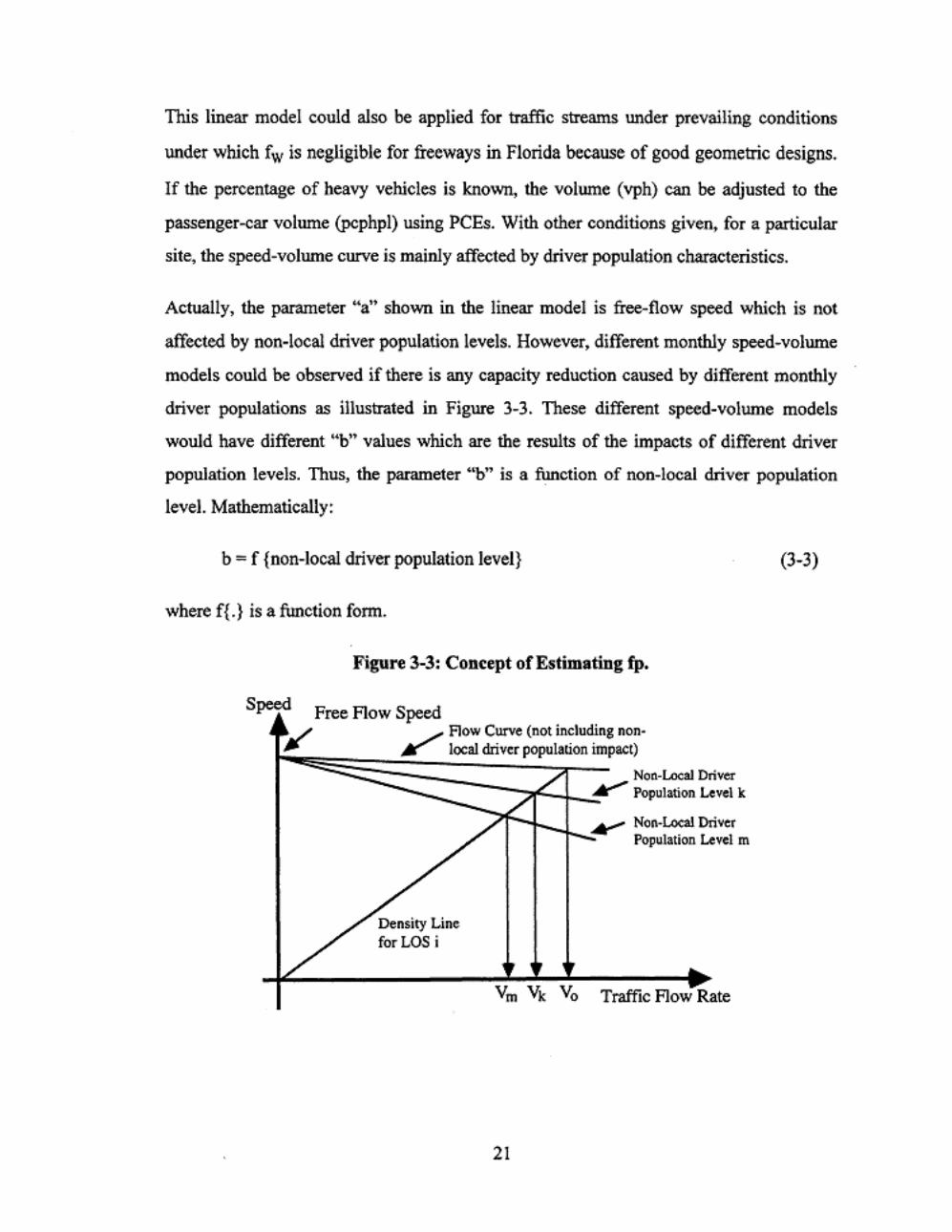
Actually, the parameter "a" shown in the linear model is free-flow speed which is not
affected by non-local driver population levels. However, different monthly speed-volume
models could be observed if there is any capacity reduction caused by different monthly
driver populations as illustrated in Figure 3-3. These different speed-volume models
would have different "b" values which are the results of the impacts of different driver
population levels. Thus, the parameter "b" is a function of non-local driver population
level. Mathematically:
b = f {non-local driver population level}
where f{.} is a function fonn.
Figure 3-3: Concept of Estimating fp.
Speed Free Flow Speed •. / _ ./ Row Curve (not including non8
r~ ... ,.'OO::::O~K~==~Ioc~al~dri;·v;e~r~ pop~ul~au[·o~n~im:pact) Non-Local Driver At"" Population Level k
......- Non-Loeal Driver Population Level m
Vm Vk Vo Traffic Flow Rate
21
(3-3)
In Figure 3-3, the density line represents a given LOS as defined by the HCM. According
to the 1994 HCM, the LOS is defined based on the traffic density. The traffic conditions
on the same density line should have the same level-of-service. Because the traffic
volwnes have already been transferred into the passenger car equivalents using fHV and fw
is negligible, the volume should be V • in the density line if there is no capacity reduction
caused by the non-local driver population. However, if non-local driver population level k
is observed, the resulting speed-volwne curve would intersect the density line at volwne
V 0 • The corresponding driver population adjustment factor, fpk• can be estimated
according to the following equation:
(3-4)
If non-local driver population level is further increased to level m, by the same concept,
the corresponding driver population adjustment factor fp.. can be estimated by the
following equation:
f. Vm pm = -v;;- (3-5)
Conceptually, a group of different non-local driver population levels would result in a
group of different speed-volume curves. For each specific speed-volume curve, a driver
population adjustment factor can be estimated. Thus, for each non-local driver population
level, a corresponding driver population adjustment factor can be estimated. 1his
conceptual method was used in this study.
Calibration of Population Adjustment Factors
There are two basic issues that had to be addressed in this study. First, from existing or
new traffic data (data type I which includes traffic flow rate, speed, and vehicle
classification), capacity reduction due to non-local driver population had to be identified
using statistical methods. Consequently, the adjustment factor fP can be estimated under
22

different conditions. Second, methods needed to be developed to estimate indices that
represent non-local driver population levels (data type II). A statistical analysis was
conducted to relate the adjustment factor f with the estimation of non-local driver p
population levels. A wide range of non-local driver population levels was needed so that
a reasonable calibration off can be reached. Figure 3-4 illustrates the principle involved p
in developing a driver population adjustment factor table.
Figure 3.4: Basic Principle of Developing Driver Population Adjustment Factors.
Data Type I D T U ata type
f p Estimation ,_ Estimation of Non-Local r- Driver Population Levels ,
I Statistical Analysis I
Final Products (Tables)
The relationships between traffic flow characteristics and driver population could be
estimated either by a cross-sectional study, comparing conditions at a variety of sites, or
by a longitudinal study at a particular site, over an extended time period.
23
CHAPTER 4: RESEARCH DATA SOURCES
Traffic Data
The FOOT permanent count traffic stations were a valuable source of freeway traffic data
in this study. These monitoring sites make use of inductive loop detectors. Data are stored
in roadside computers and transmitted to the FOOT central computer using a telemetry
system, with the data summarized in one hour time intervals. More than I 00 monitoring
sites are located throughout Florida, primarily on freeway sections and other principal
arterial highways along. the State Highway System. A significant number of the
monitoring sites include data regarding traffic volume, average vehicle speeds, vehicle
classification, and at selected weigh-in-motion sites, information about vehicle weights.
The historical traffic data collected at these stations are reported on a directional basis, for
each traffic lane, summarized in hourly intervals. The historical traffic data collected at
these stations in 1995 were the major data resource for this study.
There are many count stations along freeways in Florida, however, only ten stations
collected more than 200 days of speed, volume, and classification data for the year of
1995. Other sites could not supply sufficient records due to some problems such as
freeway construction or equipment failure. The locations of these ten stations are
presented in Figure 4-1 and Table 4-1. To evaluate the impacts of the non-local driver
population on freeway capacity, only the sites which experienced high traffic volumes
were selected for further analysis because high traffic volumes were essential to calibrate
speed-volume models.
The 1995 computerized traffic data from these ten sites was acquired from the FOOT.
These original data files were named according to the site, character (speed, volume, or
classification), traffic direction and date. The original database provided by FOOT had a
format that could not be used directly for analysis. A computer program using SAS
programming was developed to convert the original database into a readable format ready
for data analysis. Meanwhile, the vehicle classification data were employed to convert
24
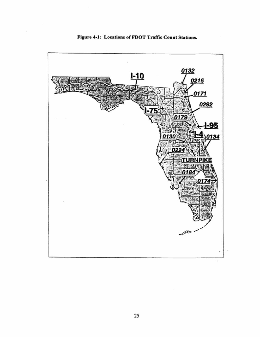
Figure 4-1: Locations ofFDOT Traffic Count Stations.
25
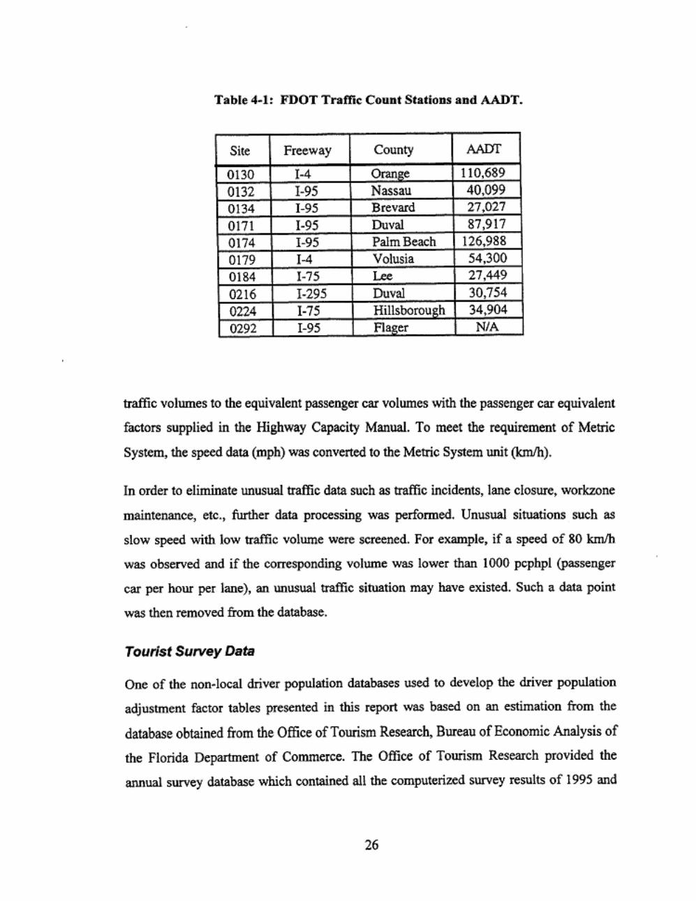
Table 4-1: FDOT Traffic CouDt StatloDs &Dd AADT.
Site Freeway County AAN
0130 1-4 Oran~~:e 110,689
0132 I-95 Nassau 40.099
0134 1-95 Brevard 27,027
0171 1-95 Duval 87,917
0174 1-95 Palm Beach 126.988
0179 1-4 Vol usia 54,300
0184 1-75 Lee 27,449
0216 1-295 Duval 30,754
0224 I-75 Hillsborou~b 34,904
0292 1-95 Aal!er N/A
traffic volwnes to the equivalent passenger car volwnes with the passenger car equivalent
factors supplied in the Highway Capacity Manual. To meet the requirement of Metric
System, the speed data (mph) was converted to the Metric System unit (kmlh).
In order to eliminate unusual traffic data such as traffic incidents, lane closure, worl<zone
maintenance, etc., further data processing was performed. Unusual situations such as
slow speed wilh low traffic volume were screened. For example, if a speed of 80 km/h
was observed and if the corresponding volume was lower than I 000 pcpbpl (passenger
car per hour per lane), an unusual traffic situation may have existed. Such a data point
was then removed from the database.
Tourist Survey Oats
One of the non-local driver population databases used to develop the driver population
adjustment factor tables presented in this report was based on an estimation from the
database obtained from the Office of Tourism Research, Bureau of Economic Analysis of
the Florida Department of Commerce . The Office of Tourism Research provided the
annual survey database which contained all the computerized survey results of 1995 and
26

monthly updates of their tourist swveys which were composed of air-visitor swveys and
auto-visitor surveys. Approximately I 0,000 person-to-person interviews were conducted
with out-of-state visitors (US and Canadian) each year by the Office of Tourism
Research. These visitors must have been in the state for at least one night and no more
than 180 nights to be classified as visitors. Commuters were not included in the surveys.
Swveys of air travelers were conducted in airport departure lounges for I!Ommercial
flights leaving Florida from thirteen major airports twice each month. Auto visitor
surveys were made on 27 roads near the Florida border each month. Only out-of-state
visitors were defined as tourists (visitors) in the swveys. On Interstate Highways (1-95, I
I 0, and l-75), swveys were conducted at the freeway rest areas closest to the Florida
border. Traffic was stopped on all other highways to interview visitors. Visitor
characteristics such as destinations, number of persons in a travel party, rental car usage,
vehicle occupancies and days of stays were recorded in the swveys.
In this study, the visitor-day was defined as the total number of days spent by a visitor
who had used a car in these areas during his/her stay. The definition of "the visitor who
had used a car" could be either an auto visitor or an air visitor who rented a car. The
visitor-day was established to better measure the impacts of visitors. It also changed the
number of visitors into the number of days they spent which should be more appropriate
in evaluations of these drivers' presence in traffic flows. The "visitor-day" is defined by
the following equation:
visitor-day= number of visitors x total days of stay
Estimation of Non-Local Driver Population Levels Using Tourist Survey Data
(4-1)
The tourist survey database was used to estimate non-local driver population levels. The
statewide tourist infonnation and the swvey database were used in the estimation of
monthly non-local driver population levels. The following equation was used to estimate
the total number of visitor-days in an area:
27
where
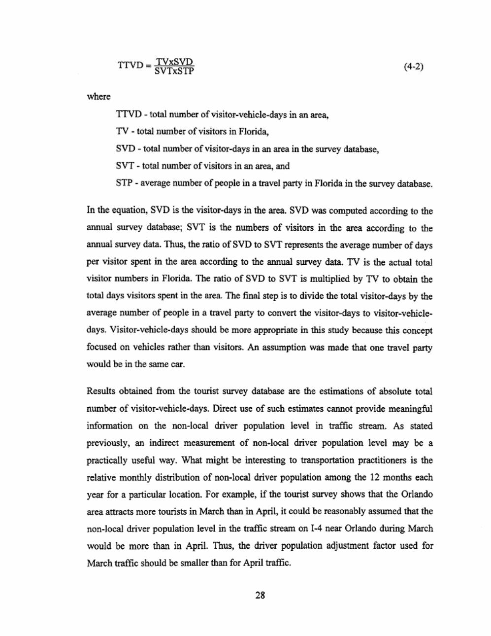
ITVD = TVxSVD SVTxSTP
TTVD -total number of visitor-vehicle-days in an area,
TV - total number of visitors in Florida,
SVD - total number of visitor-days in an area in the survey database,
SVT - total number of visitors in an area, and
(4-2)
STP - average number of people in a travel party in Florida in the survey database.
In the equation, SVD is the visitor-days in the area. SVD was computed according to the
annual survey database; SVT is the numbers of visitors in the area according to the
annual survey data. Thus, the ratio of SVD to SVT represents the average number of days
per visitor spent in the area according to the annual survey data. TV is the actual total
visitor numbers in Florida. The ratio of SVD to SVT is multiplied by TV to obtain the
total days visitors spent in the area. The final step is to divide the total visitor-days by the
average number of people in a travel party to convert the visitor-days to visitor-vehicle
days. Visitor-vehicle-days should be more appropriate in this study because this concept
focused on vehicles rather than visitors. An assumption was made that one travel party
would be in the same car.
Results obtained from the tourist survey database are the estimations of absolute total
number of visitor-vehicle-days. Direct use of such estimates cannot provide meaningful
information on the non-local driver population level in traffic stream. As stated
previously, an indirect measurement of non-local driver population level may be a
practically useful way. What might be interesting to transportation practitioners is the
relative monthly distribution of non-local driver population among the 12 months each
year for a particular location. For example, if the tourist survey shows that the Orlando
area attracts more tourists in March than in April, it could be reasonably assumed that the
non-local driver population level in the traffic stream on 1-4 near Orlando during March
would be more than in April. Thus, the driver population adjustment factor used for
March traffic should be smaller than for April traffic.
28
In the study, the estimate of non-local driver population levels by area and by month
developed from the tourist surveys was used as a proxy for direct observations of vehicles
in order to indirectly estimate the non-local driver population levels in the traffic stream.
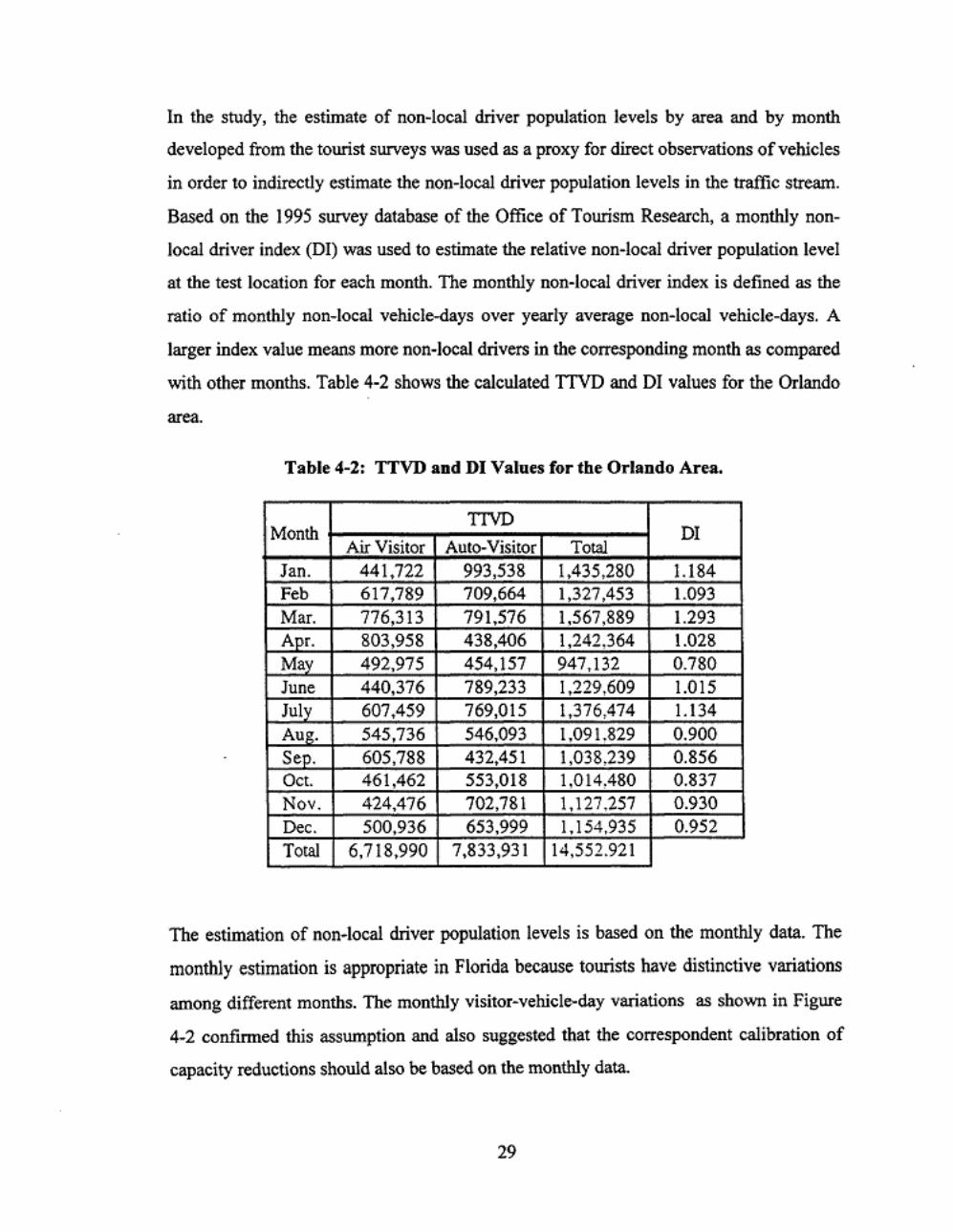
Based on the 1995 survey database of the Office of Tourism Research, a monthly non
local driver index (DI) was used to estimate the relative non-local driver population level
at the test location for each month. The monthly non-local driver index is defined as the
ratio of monthly non-local vehicle-days over yearly average non-local vehicle-days. A
larger index value means more non-local drivers in the corresponding month as compared
with other months. Table 4-2 shows the calculated TTVD and DI values for the Orlando
area.
Table 4-2: TTVD and DI Values for the Orlando Area.
Month TIVD
DI Air Visitor Auto-Visitor Total
Jan . 441,722 993,538 1,435,280 Ll84 Feb 617,789 709,664 1,327,453 1.093 Mar. 776,313 791,576 1.567,889 1.293 Apr. 803,958 438,406 1,242,364 1.028 May 492.975 454,157 947,132 0.780 June 440,376 789,233 1,229,609 1.015 July 607,459 769,015 1,376,474 1.134 Aug. 545,736 546,093 1.09 1,829 0.900 Sep. 605,788 432,451 1,038,239 0.856 Oct. 461,462 553,018 1,014.480 0.837 Nov. 424,476 702,781 1.127,257 0.930 Dec. 500,936 653,999 1.154.935 0.952 Total 6,718,990 7,833,931 14,552.921
The estimation of non-local driver population levels is based on the monthly data. The
monthly estimation is appropriate in Florida because tourists have distinctive variations
among different months. The monthly visitor-vehicle-day variations as shown in Figure
4-2 confirmed this assumption and also suggested that the correspondent calibration of
capacity reductions should also be based on the monthly data.
29

Figure 4-2: Dl Values for Different Moaths in Orlando Area.
1.5
1.4
1.3
1.2
1.1
-Cl 1.0
0.9
o.a
0.7
0.6
0.5 1 2 3 4 5 6 7 a 9 1 0 1 1 12
Month
Estimation of Non-Local Driver Population Levels Using Traffic Data
Another method for indirect measurement of non-local driver population levels is to look
at the traffic volume itself. Traffic data is relatively easier 1o obtain than the tourist data
because FDOT bas the full access to traffic count stations located on Florida freeways.
Traffic volumes vary at different locations and among different months in the same site.
It is also true that traffic volumes vary according to different hours and days of the week.
As evidenced by the literature reviews, particularly the work by Sharma (1986), the
volume variations have been used to estimate traffic characteristics. It is reas<lnable to
assume that these kinds of volume variations are associated with different non-local
driver population levels. For example, highways near tourist attractions have higher non
peak traffic volume than highways in business areas where most drivers are commuters
traveling during peak hours. Also, traffic volumes near tourist attractions are higher
during peak tourist seasons than the rest of the year. Using this concept, some indices can
be developed to indirectly indicate the relative distribution ofnon-local driver population
on a freeway section.
30

In this study, some indices were established to measure the traffic variations caused by
different driver population levels. These indices should correlate with volume variations
and driver population levels, and they also should have specific definitions and clear
calculation procedures so that they could be easily used by general practitioners. Three
different volume indices were established in this study, namely monthly factor (MF),
weekly factor (WF), and daily factor (OF).
MF is the ratio of the monthly average daily traffic (MADn to the annual average daily
traffic (AADn. It is believed that a major portion of the additional traffic observed
during peak seasons is made up of non-local drivers or tourists. WF is the ratio of
monthly average Sunday traffic (V """) to monthly average weekday traffic (V W<t). For
better comparison, the weekdays were defined as Tuesday, Wednesday, and Thursday to
eliminate recreational drivers as far as possible. OF is the ratio of monthly average
afternoon non-peak traffic (Vpm) to monthly average morning peak traffic (V ..,.). Visitors
would travel not only in peak hours but also in non-peak hours, and many visitors would
try to avoid peak traffic. As a result, non-peak hour traffic has more non-local drivers
than peak hour traffic. In this study 7am-8am was defined as the morning peak hour, and
I pm-2prn as the afternoon non-peak hour.
The speed-volume data obtained from FOOT traffic count stations was used to compute
MF, WF, and OF for each different site. All the abnormal observations and holidays were
deleted from the computation. The detailed definitions of MF, WF, and OF are shown as
follows.
MF - MAOT - AADT
Vt-2pm OF = V7 - 8am
31
(4·3)
(4-4)
(4·5)

where
VJ-2pm DF= V7-8am (4·6)
MF, WF, OF= monthly, weekly, and daily factors, respectively,
MADT = monthly average daily traffic,
AADT = annual average daily traffic,
V ~ = monthly average Sunday traffic,
V,.. =monthly average weekday (Tuesday, Wednesday and Thursday) traffic,
v,.,,.. = monthly average weekday afternoon non-peak hour (lpm-2pm) traffic,
and
V '"'"' = monthly average weekday morning peak hour (7am-8am) traffic.
The detailed calculation results are shown in Table 4-3 and graphically presented in
Figures 4-3, 4-4, and 4-5. In Table 4-3, MF and WF were based on daily directional
volumes, not hourly lane volumes. According to their definitions, higher MF, WF, and
DF could be the results of the higher level of non-local driver population.
Figure 4-3: MF Values for Different Months in Orlando Area (WB and Lane 1 only).
1.20.-----------------------, 1.15
1.10
1.05
1.00
0.95
0.90
0.85
32

1<.
:3:
"-Cl
Figure 4-4: WF Values for Different Months in Orlando Area (WB and Lane 1 Only).
·us
1.10
1.05
1.00
0 .95
0 .90
0 .85
0.80
0.75 1 2 3 4 5 6 7 8 9 10 1 1
Month
Figure 4-S: DF Values for Different Montbs in Orlando Area (WB and Lane l Only).
1.00
0.95
0.90
0.85
0.80
0.75
0 .70
0 .65
0.60 1 2 3 4 5 6 7 ·a· 9 10
Month
33
1 1
1 2
12
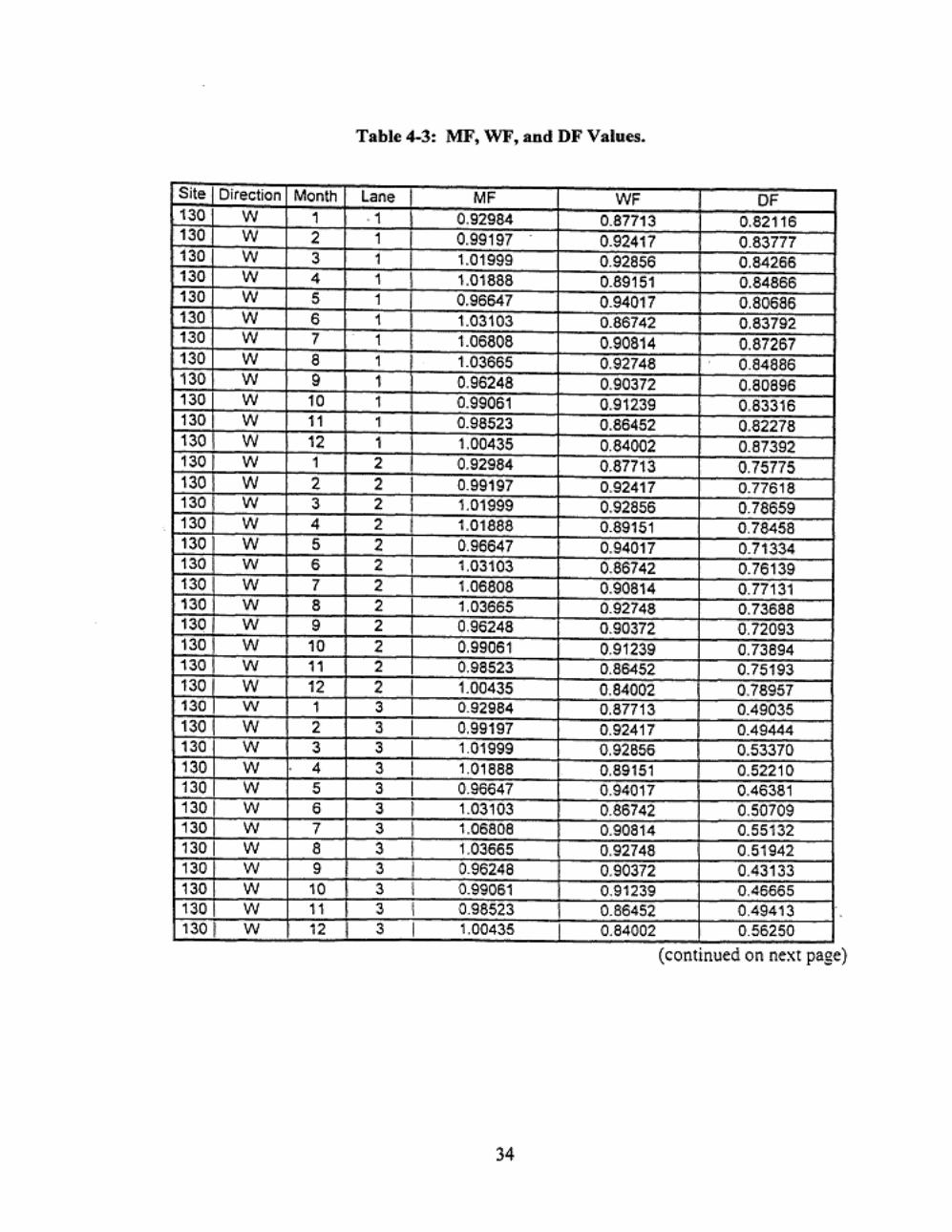
Table 4-3: MF, WF, and DF Values.
Site Direction Month Lane MF WF OF 130 w 1 . 1 0.92984 0.87713 0.82116 130 w 2 1 0.99197 . 0.92417 0.83777 130 w 3 1 1.01999 0.92856 0.84266 130 w 4 1 I 1.01888 0.89151 0.84866 130 w 5 1 0.96647 0.94017 0.80686 130 w 6 1 1.03103 0.86742 0.83792 130 w 7 1 1.06808 0.90814 0.87267 130 w 8 1 I 1.03665 0.92748 0.84886 130 w 9 1 0.96248 0.90372 0.80896 130 w 10 1 0.99061 0.91239 0.83316 130 w 11 1 0.98523 0.86452 0.82278 130 w 12 1 1.00435 0.84002 0.87392 13o I w 1 2 0.92984 0.87713 0.75775 130 I w 2 2 I 0.99197 0.92417 0.77818 130 I w 3 2 I 1.01999 0.92856 0.78659 130 w 4 2 1.01888 0.89151 0.78458 130 w 5 2 0.96647 0.94017 0.71334 130 w 6 2 I 1.03103 0.66742 0.76139 130 w 7 2 I 1.06808 0.90814 0.77131 130 w 8 2 I 1.03665 0.92748 0.73688 13Q w 9 2 0.96248 0.90372 0.72093 130 w 10 2 0.99061 0.91239 0.73894 130 w 11 2 0.98523 0.86452 0.75193 130 w 12 2 I 1.00435 0.84002 0.78957 130 w 1 3 I 0.92984 0.87713 0.49035 130 w 2 3 I 0.99197 0.92417 0.49444 130 w 3 3 I 1.01999 0.92856 0.53370 130 w 4 3 I 1.01888 0.89151 0.52210 130 w 5 3 I 0.96647 0.94017 0.46381 130 w 6 3 I 1.03103 0.86742 0.50709 130 w 7 3 I 1.06808 0.90814 0.55132 130 I w 8 3 I 1.03665 0.92748 0.51942 130 w 9 3 I 0.96248 0.90372 0.43133 130 w 10 3 I 0.99061 0.91239 0.46665 130 w 11 3 I 0.98523 0.86452 0.49413 130 I w 12 3 I 1.00435 0.84002 0.56250 .
(conttnued on next page)
34

Table 4-3: MF, WF, and DF Values (continued).
Site Direction Month Lane MF WF OF 171 N 1 1 0.93851 0.51433 0.71924 171 N 2 1 0.98652 0.57342 0.72244 171 N 3 1 1.07692 0.63853 0.78575 171 N 4 1 1.05429 0.61750 0.76084 171 N 5 1 1.01168 0.55605 0.73405 171 N 6 1 1.03375 0.55655 0.75432
171 N 7 1 0.99447 0.60251 0.80143
171 N 8 1 1.02060 0.57265 0.73567
171 N 9 1 0.95916 0.54995 0.70563 171 N 10 1 0.96073 0.55608 0.70205
171 N 11 1 0.97215 0.52639 0.75176 171 N 12 1 0.96407 0.54490 0.78873
171 N 1 2 0.93851 0.51433 0.56771
171 N 2 2 0.98652 0.57342 0.59595
171 N 3 2 1.07692 0.63853 0.69436
1'71 N 4 2 1.05429 0.61750 0.67175
171 • N 5 2 1.01168 0.55605 0.61759
171 N 6 2 1.03375 0.55655 0.62451
171 N 7 2 0.99447 0.60251 0.68129
171 N 8 2 1.02060 0.57265 0.61638
171 N 9 2 0.95916 0.54995 0.58207
171 N 10 2 0.96073 0.55608 0.58827
174 N 1 1 1.01433 0.64691 0.59672
174 N 2 1 1.07098 0.70993 0.59860
174 N 3 1 1.07834 0.71917 0.65017
174 N 4 1 1.04351 0.69725 0.58864
174 N 5 1 0.99870 0.67247 0.57560
174 N 6 1 0.99361 0.65349 0.59452
174 N 7 1 0.95242 0.69002 0.62706
174 N 8 1 0.94794 0.72865 0.59550
174 N 9 1 0.96124 0.62162 0.55585
174 N 10 1 0.96181 0.69095 0.57744
174 N 1 2 1.01433 0.64691 0.88448 .
174 N 2 2 1.07098 0.70993 0.89579
174 N 3 2 1,07834 0.71917 0.91554
174 N 4 2 1.04351 0.69725 0.84163
174 N 5 2 0.99870 0.67247 0.85076
174 N 6 2 0.99361 0.65349 0.89007
174 N 7 2 0.95242 0.69002 0.94062
174 N 8 2 0.94794 0.72865 I 0.87399
174 N 9 2 0.96124 0.62162 I 0.87650
174 N 10 2 0.96181 0.69095 0.86368
174 N 1 1 3 1.01433 0.64691 1.07869
(conttnued on next page)
35

Table 4-3: MF, WF, aod DF Values (eootioued).
Site Direction Month Lane MF WF OF 174 N 2 3 1.07098 0.70993 1.11648 174 N 3 3 1.07834 0.71917 1.08308 174 N 4 3 1.04351 0.69725 1.01571 174 N 5 3 0.99870 0.67247 1.09741 174 N 6 3 0.99361 0.65349 1.10434 . 174 N 7 3 0.95242 0.69002 1.15262 174 N 8 3 0.94794 0.72865 1.099<41 174 N 9 3 0.96124 0.62162 1.06768 174 N 10 3 0.96181 0.69095 1.07874 174 s 1 1 0.95063 0.67372 0.70013 174 s 2 1 1.07071 0.74638 0.67767 174 s 3 1 1.09665 0.76384 0.77191 174 s 8 1 0.94147 0.74025 0.84010 174 s 9 1 0.86861 0.64747 0.81804 174 s 11 1 1.05581 0.70305 0.96001 174 s 12 1 1.01383 0.68973 0.91887 174 s 1 2 . 0.95063 0.67372 0.84099 174 s 2 2 1.07071 0.74638 0.76833 174 s 3 2 1.09665 0.76384 0.74860 174 s 8 2 0.94147 0.74025 0.86793 174 s 9 2 0.86861 0.64747 0.84363 174 s 11 2 1.05581 0.70305 1.12907 174 s 12 2 1.01383 0.68973 0.99429 174 s 1 3 0.95063 0.67372 0.82355 174 s 2 3 1.07071 0.74638 0.81322 174 s 3 3 1.09665 0.76384 0.70444 174 s 8 3 0.94147 0.74025 0.69634 174 s 9 3 0.86861 0.64747 0.65268 174 s 11 3 1.05581 0.70305 0.90603 174 s 12 3 1.01383 •) .68973 0.84565
36

CHAPTER 5: DEVELOPMENT OF DRIVER POPULATION ADJUSTMENT FACTOR TABLE BASED
ON TOURIST SURVEY DATA
The purpose of the research effort swnmarized in this chapter was to evaluate the impact
of non-local driver population on freeway traffic capacity. Based on the results of the
evaluation, a driver population adjustment factor table was developed. Since the 1995
traffic database from FOOT traffic count stations included 12-month traffic data and the
survey database from the Office of Tourism Research provided information to estimate
monthly non-local driver indices which represented the relative non-local driver
population level for each month during 1995, the basic principle employed in the research
was to compare the volume-speed curve differences among the 12 months.
Tourist survey data and traffic count data were reviewed before further statistical analysis
was performed. It was found that some count stations did not show high traffic volumes,
and some areas did not present good tourist survey results. In the effort to develop driver
population adjustment factors based on the Office of Tourist Research data, the Orlando
area was selected because good tourist survey results were available and the whole year
traffic counts and high traffic volumes were included in the database. Conceptually, the
data set which covers one area is enough for the study purpose if the data set covers all
possible tourist seasons and all possible peak and non-peak seasons.
Modeling Procedure and Results
As stated in Chapter 3, a speed-volume curve under the condition of stable traffic can be
described by a linear equation. Practically, a driver population adjustment factor can be
applied only if the traffic is stable. The factor is meaningless if forced-flow traffic exists.
Therefore, to analyze the impact of non-local driver population on traffic capacity, the
linear equation can be used to represent speed-volume curves. To further confirm this
assumption, three speed-volume data sets were randomly selected from the database and
are shown in Figures 5-1, 5-2, and 5-3. From these figures, it can be concluded that a
37

~ -~ "" ~ "8 !:L "' "" = ·--e & 0
" "" .. -!I <
Figure 5-1: Relationship between Volume and Speed (1-4 WB Laue 1, January 1995, Orlando, Site: 0130).
1Wr-----~--~----------------------~
Speed = 96.04 - 4.3e-3Volume R"2 = 0.470
o~~~~~~~~~--~--~~~~~~
0 200 400 600 800 I 000 1200 1400 1600 1800 2000
120
100
80
60 r
40 r
20
Volume (pcph)
Figure 5-2: Relationship between Volume and Speed (1-4 WB L aue 2, October 1995, Orlando, Site: 0130).
Speed= 104.75- 2.9e-3Vo1ume R"2 = 0.215
o~~~-L~~~~~~~~~~~~~~
om 400 600 o 1~ 1200 1~160018002~
Volume (pcph)
38
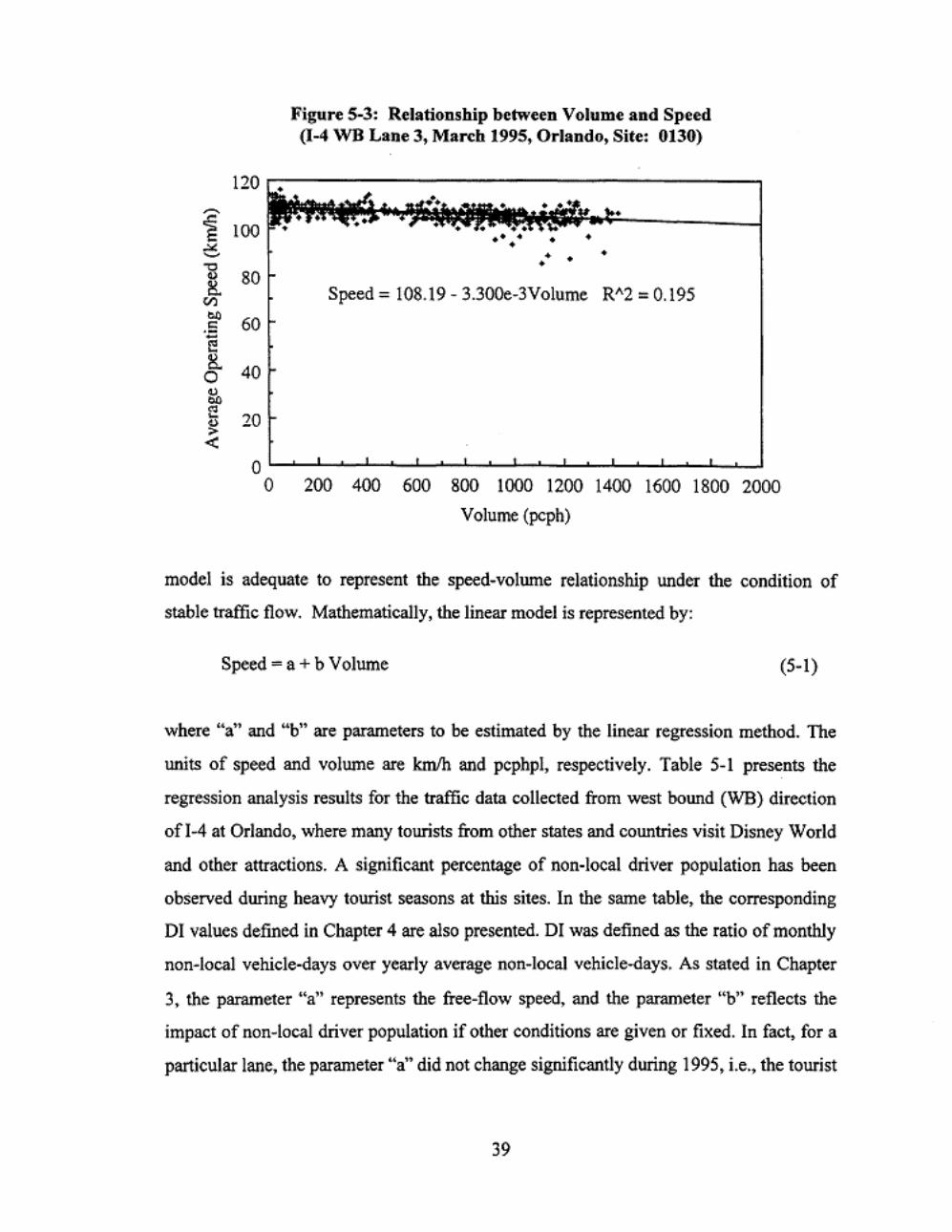
~ ~ 20 <
Figure S-3: Relationship between Volume and Speed (l-4 WB Lane 3, March 1995, Orlando, Site: 0130)
• • • •
Speed= 108.19 - 3.300e-3Volume R"2 = 0.195
o~~~-L~~~~~~~~~~L-~~_J
0 200 400 600 800 1000 1200 1400 1600 1800 2000
Volume (pcph)
model is adequate to represent the speed-volwne relationship under the condition of
stable traffic flow. Mathematically, the linear model is represented by:
Speed =a + b Volwne (5-1)
where "a" and "b" are parameters to be estimated by the linear regression method. The
units of speed and volwne are kmlh and pcphpl, respectively. Table 5-1 presents the
regression analysis results for the traffic data collected from west bound (WB) direction
ofl-4 at Orlando, where many tourists from other states and countries visit Disney World
and other attractions. A significant percentage of non-local driver population has been
observed during heavy tourist seasons at this sites. In the same table, the corresponding
01 values defined in Chapter 4 are also presented. 01 was defined as the ratio of monthly
non-local vehicle-days over yearly average non-local vehicle-days. As stated in Chapter
3, the parameter "a" represents the free-flow speed, and the param.eter "b'' reflects the
impact of non-local driver population if other conditions are given or fixed. In fact, for a
particular lane, the parameter "a" did not change significantly during 1995, i.e._, the tourist
39
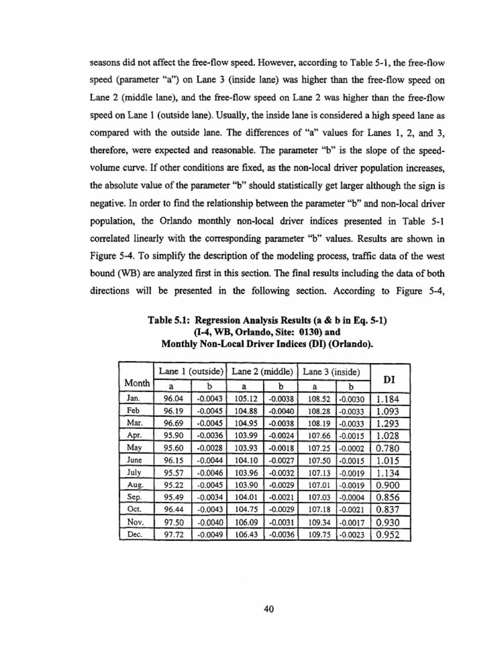
seasons did not affect the free-flow speed. However, according to Table 5-l, the free-flow
speed (parameter "a") on Lane 3 (inside lane) was higher than the free-flow speed on
Lane 2 (middle lane), and the free-flow speed on Lane 2 was higher than the free-flow
speed on Lane I (outside lane). Usually, the inside lane is considered a high speed lane as
compared with the outside lane. The differences of "a" values for Lanes I, 2, and 3,
therefore, were expected and reasonable. The parameter "b" is the slope of the speed
volume curve. If other conditions are fixed, as the non-local driver population increases,
the absolute value of the parameter "b" should statistically get larger although the sign is
negative. In order to fmd the relationship between the parameter "b" and non-local driver
population, the Orlando monthly non-local driver indices presented in Table 5-1
correlated linearly with the corresponding parameter "b" values. Results are shown in
Figure S-4. To simplify the description of the modeling process, traffic data of the west
bound (WB) are analyzed first in this section. The final results including the data of both
directions will be presented in the following section. According to Figure S-4,
Table 5.1: Regression Analysis Results (a & bin Eq. 5·1) (1-4, WB, Orlando, Site: 0130) and
Monthly Non-Local Driver Indices (DI) (Orlando).
Lane I (outside) Lane 2 (middle) Lane 3 (inside) DI Month a b a b a b
Jon. 96.04 ·0.0043 105.12 -0.0038 108.52 ·0.0030 1.184 Feb 96.19 ·0 .0045 104.88 ·0.0040 108.28 -0.0033 1.093 Mar. 96.69 ·0.0045 104.95 -0.0038 108.19 -0.0033 1.293 Apr. 95.90 ·0.0036 103.99 .().0024 107.66 -0.0015 1.028 May 95.60 ·0.0028 103.93 -0.0018 107.25 .().0002 0.780 June 96.15 -0.0044 104.10 -0.0027 107.50 -0.0015 1.015 July 95.57 -0.0046 103.96 ·0.0032 107.13 -0.0019 1.134 Aug. 95.22 ·0.0045 103.90 ·0.0029 107.01 -0.0019 0.900 . Sep. 95.49 -0.0034 104.01 ·0.0021 107.Q3 -0.0004 0.856 Oc<. 96.44 -0.0043 104.75 -0.0029 107.18 -0.0021 0.837 Nov. 97.50 -0.0040 106.09 ·0.0031 109.34 -0.0017 0.930 Dec. 97.72 ·0.0049 106.43 .().0036 109.75 ·0.0023 0.952
40

Figure S-4: Statistical Relationship between Parameter " b" and Montbly Non-Local Driver Index (DI) (1-4 WB, Orlando, Site: 0130).
0.000 • -0.001
..().002
:0 ' ~ -0.003 <> -., E ::
{;,! -0.004
·0.005
-0.006
-0.007 0.7
• Lane I
o Lane2
• Lane3
0.8
• • • • b = -·2.1076e·3 · 2.042le-3 DI R"2 = 0.275
b = 2.9630e-4 - 3.3207e-3 DI R"2 = 0.531
b = 2.9859e-3 · 4.910 le-3 DI R"2 = 0.580
0.9 1.0 1.1 1.2 1.3 Monthly !'<on-Local Driver Index (DI)
1.4
statistically, the parameter "b" values listed in Table 4-1 had a certain correlation with the
non-local driver populaJion levels. As the non-local driver population increased or as DI
increased, the absolute parameter "b" values of all three lanes increased correspondingly.
This confirmed that the parameter "b" could be used to reflect the impact of non-local
driver population on traffic capacity. The larger the absolute parameter "b" value, the
more the non-local driver population increased. In general, based on Figure 5-4, one can
demonstrate statistically that as the non-local driver population in the traffic stream
increases, traffic capacity decreases correspondingly.
Another important fact to be noted in Figure 5-4 is that the absolute "b" value results
from the outside lane (Lane I) were statistically larger than those from the middle lane
(Lane 2) and inside lane (Lane 3). The inside lane had the lowest absolute "b" values for
given monthly non-local driver indices. The main reason may be that most non-local
drivers who would cause the reduction in lane capacity might be traveling in the outside
lane with relatively slower operating speeds because these drivers were not familiar with
41

the roadway or they were not commuters. This category of drivers might choose the
middle lane too. However, fewer non-local drivers would choose the inside lane with
higher operating speeds, as compared with outside and middle lanes. This indicates that
non-local driver population may not distribute uniformly among lanes, and the impacts of
non-local driver population in different lanes may be different.
Although a linear equation was used in Figure 5-4, the rate of change of the parameter
"b" with respect to DI may not be constant in practical cases. This rate is relatively
smaller when DI is small than when DI is large. A second-order polynomial model could
be used to represent such a statistical relationship between "b" and 01. Meanwhile, to
represent statistically the impact of non-local driver population as a whole, the monthly
volume-speed curves from Lanes I, 2, and 3 were combined without distinguishing lanes.
Mathematically,
B(i) = bl(i)+b2~i)+b3(i) (5-2)
and
A(i) = al(i)+a2ji)+a3(i) (5-3)
where bl(i), b2(i), and b3(i) are the parameter "b" values for month i (i = I, 2, ... , 12),
representing Lanes I, 2, and 3, respectively, and al(i), a2(i), and a3(i) are the parameter
"a" values for month i, representing Lanes I, 2, and 3, respectively. In fact, A(i) is
monthly free-flow speed of the WB traffic. and is not affected by non-local driver
population. Therefore, an average value of A(i) (i =1 , 2, ... , 12) was used in this study, or
12
A= t~LA(i) j;:;}
Based on Table 4-1 , the value of A was calculated; A= !03 km/hour.
42
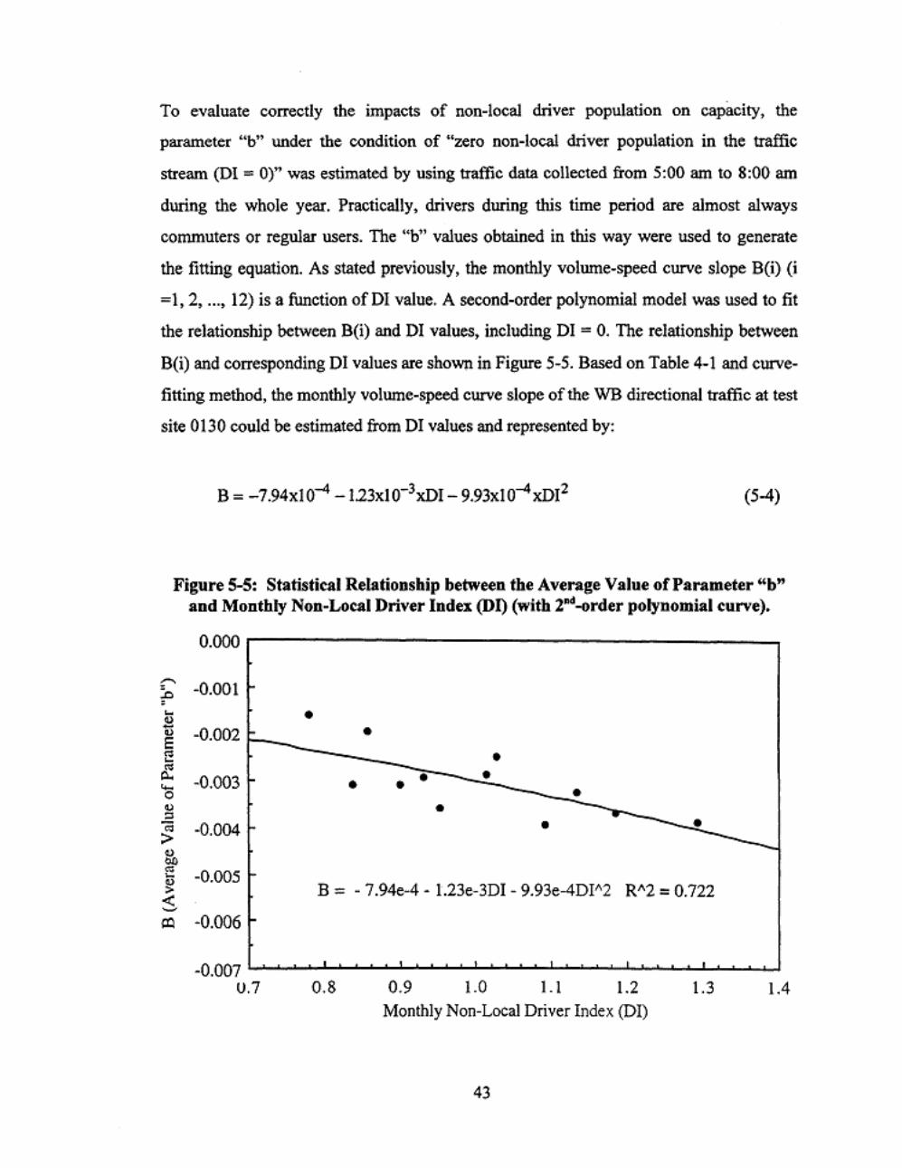
To evaluate correctly the impacts of non-local driver population on capacity, the
parameter "b" under the condition of "zero non-local driver population in the traffic
stream (Dl = 0)" was estimated by using traffic data collected from 5:00 am to 8:00 am
during the whole year. Practically, drivers during this time period are almost always
commuters or regular users. The "b" values obtained in this way were used to generate
the fining equation. As stated previously, the monthly volume-speed curve slope B(i) (i
=I, 2, ... , 12) is a function ofDI value. A second-order polynomial model was used to fit
the relationship between B(i) and DI values, including Dl = 0. The relationship between
B(i) and corresponding DI values are shown in Figure 5-5. Based on Table 4-1 and curve
fitting method, the monthly volume-speed curve slope of the WB directional traffic at test
site 0130 could be estimated from DI values and represented by:
(5-4)
Figure 5-S: Statistital Relationship between the Average Value of Parameter "b" and Monthly Non-Lotal Driver Index (DI) (with 2"-order polynomial curve).
0.000
~
' .J:> -0.001 ' -" iS -0.002 E
• • ., - • rf. -0.003 .... 0 • • • • • .. "' -;;; -0.004 > • • • 0 01)
e -0.005 r-~ < ~
B = - 7.94e-4- 1.23e-3DI- 9.93e-4Dl'2 R"2 = 0.722
lQ -0.006 r-
-0.007 ' 0 .7 0.8 0.9 1.0 1.1 1.2 1.3 1.4
Monthly Non-Local Driver Index (DI)
43

with a correlation coefficientof0.122 (R2 = 0.122). The final equation to characterize
the average impact of non-local driver population on the freeway segment (all lanes)
capacity can be expressed as follows:
Speed ~ A+ B Volume (5-5)
or
Based on Equation (5-6), with other prevailing conditions fixed, average operating speed
is a function of non-local driver population level and average lane volume. As non-local
driver population increases, the average operating speed decreases, resulting in decreased
capacity under prevailing conditions.
Figure S-6 presents a group of speed-volume curves with each curve representing a
particular monthly non-local driver index. nus figure, with data collected from 1-4 West
Bound in the Orlando area, is based on Equation (S-6). The impact of non-local driver
population can be assessed graphically by reviewing this figure.
Figure 5.6: Impact of Non-Local Driver Population on Avenge Operating Speed (1-4 WB, Orlando, Site: 0130).
105 01:0.0
~ 01=.6
01=.8
-.......:: ~ t;::; 01=1.0 - 01=1.2 ~-......... I-.... '""- • 01=1.4 r---..-- ..._........,
01=1.6 r----..: 01=1.8
........... 0 01=2.0 01=2.2
Dl=2.4
80 0 200 ~ ~ 8001~1D14001~1800~0
Volume (pcph)
44

~
More Generalized Results
The same procedure described previously was applied to the East Bound lanes of 1-4
located in Orlando to obtain more general speed-volume curves from the impacts of the
non-local driver population. In fact, for each direction of interstate freeway at each
location, a group of speed-volume curves similar to those in Figure 5-6 can be obtained to
represent the non-local driver population impacts on average lane capacity. According to
the study results, the difference between the two groups of speed-volume curves of both
directions was very small and can be even neglected. In this study, these curve groups
resulting from each direction of l-4 in Orlando were averaged. The final equation
representing speed-volume curves with the impact of non-local driver population is
presented below:
Speed= 102 + ( -6.82xl0-4 -1.75xl0-3xDI- 8.99xl0-4xDI2 ) Volume (5-7)
This equation represents a general situation, because the data used to develop the above
equation were collected from both directions of 1-4 at Orlando. Consequently, Figure 5-7
presents a group of speed-volume curves developed from the data.
!OS
Figure 5-7: Impact of Non-Local Driver Population on Average Operating Speed (1-4 Both Directions, Orlando, Site: 0130).
DI=O.O
] 100
~ Dl=.6
• DI=.8 ~
1 95 <I)
eJ) c -~ 0. 90 0
" bO e " > <
85
b
~ '-- ~:-, -...., /"--.._.......__, 0 ............. ---.. ~----~ ~ t'-----
.............
200 400 600 8001000120014001600 18002000
Volume (pcph)
45
0
DI=l.O
DI=1.2 DI=l.4
Dl=1.6 DI=l.8
Dl=2.0 Dl=2.2
Dl=2.4

Estimate of Driver Population Factors Based on Test Site 0130
According to 1994 HCM, freeway LOS is based on vehicle density. Under ideal
conditions, average vehicle operating speeds on basic freeway sections are relatively
insensitive to traffic flow rates up to LOS E. However, under prevailing conditions,
average operating speeds do decrease as traffic flow rates increase. This is true
particularly when a significant population of non-local drivers exists in the traffic. stream.
To quantify the impacts of non-local driver population on freeway capacity, average
service flow rates at LOS B, C, and 0 were assessed in this study. Based on the definition
and method of defining LOS on the speed-volume curve presented in 1994 HCM, a line
starting from the origin and crossing volume-speed curves can be used to fmd
corresponding volumes with given level of service. Figure 5-8 presents the volume-speed
curves based on Figure 5-7 and one density lines representing LOS C. The density lines
representing LOS B and 0 can also be plotted in the same figure with the same way.
Because these curves were obtained from the data collected at the given test site, the
differences between these curves can be related to different monthly non-local driver
105
Figure 5-8: Estimation of Driver Population Adjustment Factors (1-4 Both Directions, Orlando, Site: 0130).
~ •
.......; :--.. ...., --......._..........., ~ ...... ...., ................. r-....
'IS N (:i4 l\1' ~ :-----....,
" ·! .........., •
80 0 200 400 600 800 1000 1200 1400 1600 1800 200
.................. 0
Volume (pcph)
46
01=0.0
01=.6 01=.8
01=1.0 01=1.2 01=1.4
01=1.6
01=1.8 01=2.0
01=2.2 01=2.4
LOSC
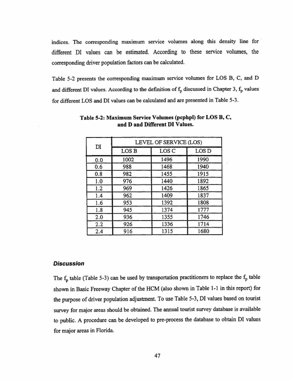
indices. The corresponding maximum service volumes along this density line for ·
different DI values can be estimated. According to these service volumes, the
corresponding driver population factors can be calculated.
Table 5-2 presents the corresponding maximum service volumes for LOS B, C, and 0
and different 01 values. According to the definition of~ discussed in Chapter 3, fp values
for different LOS and 01 values can be ealculated and are presented in Table 5-3.
Table S-2: Maximum Service Volumes (pcphpl) for LOS B, C, and D and Different Dl Values.
DI LEVEL OF SERVICE (LOS)
LOSB LOSC LOSO
0.0 1002 1496 1990 0.6 988 1468 1940 0.8 982 1455 1915 1.0 976 1440 1892 1.2 969 1426 1865 1.4 962 1409 1837 1.6 953 1392 1808 1.8 945 1374 1777 2.0 936 1355 1746 2.2 926 1336 1714 2.4 916 1315 1680
Discussion
The fp table (Table 5-3) can be used by transportation practitioners to replace the fp table
shown in Basic Freeway Chapter of the HCM (also shown in Table 1-1 in this report) for
the purpose of driver population adjustment. To use Table 5-3, DI values based on tourist
survey for major areas should be obtained. The annual tourist survey database is available
to public. A procedure can be developed to pre-process the database to obtain 01 values
for major areas in Florida.
47

Table S-3: Driver Population Adjustment Factors for Different Levels of Service, Based on Orlando Conditions
DI LEVEL OF SERVICE (LOS) Average LOSB LOSC LOSD
0.6 0.986 0.981 0.975 0.981 0.8 0.980 0.973 0.962 0.972 1.0 0.974 0.963 0.951 0.963 1.2 0.967 0.953 0.937 0.952 1.4 0.960 0.942 0.923 0.942 1.6 0.951 0.930 0.909 0.930 1.8 0.943 0.918 0.893 0.918 2.0 0.934 0.906 0.877 0.906 2.2 0.924 0.893 0.861 0.893 2.4 0.914 0.879 0.844 0.879
The results presented in this chapter are applicable to the areas with major tourist
attractions. For a particular area with DI value available, Table 5-3 can be used to find the
driver population adjustment factor to adjust freeway capacity in the area. If there is no
DI value for the particular area, DI value for au area with similar social/economic aod
tourist attraction scopes to that area could be used to adjust freeway capacity at that area.
The results might not be applicable to the areas with significant through traffic but few
tourist attractions because the areas with significant through traffic may not result in
adequate DI estimations. Only the areas with tourist traffic origins or destinations could
be considered for the application of the results presented in this chapter.
From Table 5-3, it can be concluded that non-local driver population may have more
impacts on the traffic stream with worse LOS as comparid with better LOS. In fact, as
traffic density increases, the interactions between vehicles may be more sensitive.
However, practically, the average fP values shown in Table 5-3 can be used without
distinguishing LOS.
48

CHAPTER 6: DEVELOPMENT OF A DRIVER POPULATION ADJUSTMENT FACTOR TABLE
BASED ON TRAFFIC CHARACTERISTICS
Infonnation on relative non-local driver population levels may be inferred from traffic
characteristics such as traffic variations among different months, different days, or
different hours. The basic assumption is that commuter traffic or regular local users of a
freeway section are relatively consistent and that monthly, daily, and hourly variations in
traffic are somewhat related to non local drivers. Based on such an assumption, the
monthly factor, weekly factor, and daily factor were developed in the study to indirectly
represent the relative non-local driver population levels in each month. The main benefit
of using these factors is that it is unnecessary to directly identifY non-local driver
population levels, a fonnidable task. Traffic data collected through traffic count stations
can be used to indirectly represent non-local driver population level.
As stated in Chapter 4, due to limitations associated with other traffic count stations, only
three sites were selected for this study. Two primary criteria limited the sites suitable for
analysis: (I) a requirement that at least 200 days of "good" data be available, and (2)
since the methodology was based on calibrating localized speed-volume curves, it was
necessary that high traffic volumes, in the LOS C,D, and E ranges be observable. The
three sites were 1-4 in Orlando (site 0130), 1-95 in West Palm Beach (site 0174), and 1-95
in Jacksonville (site 0171). Data from these sites cover almost the whole year traffic,
representing typical tourist seasons.
Monthly Factors, Weekly Factors, and Daily Factors
Monthly factor
Ideally, if there were no non-local drivers in the traffic stream, monthly average daily
traffic for each month would show modest variations, reflective of school closings and
family vacation schedules. However, since non-local driver population levels in different
49

months are quite different, monthly average daily traffic is also quite different
Conceptually, the following equation can be used to describe this difference:
where
MADTi = Vi + Ui (6-1)
MADTi =monthly average daily traffic for month i (i = I, 2, ... , 12)
Vi= proportion of MADTi for regular users or commuters for month i (i = I, 2,
... , 12)
Ui = proportion of MADTi for non-local driver population for month i (i = I, 2,
... , 12)
To analyze the relative non-local driver population levels in different months, Vi could be assumed constant across the 12 months, or
Vi = V (i=l,2, ... ,12) (6-2)
where V is a constant. Annual average daily traffic (AAD1) can be calculated by the
following equation:
12 12 12 12
AADT= AIMADTi = -h<IVi+ IUi) = v + lhiUi i:l i=l i=l i=l
(6-3)
According to the definition ofMF (monthly factor) defined in Chapter 4, MFi (i =1, 2, ... ,
12) ean be calculated by the following equation:
MFi = MAD'fi = v + YJ (i = I, 2, ... , 12) AAD V+...!..Lui
12 i•l
(6-4)
From the above equation, it can be understood that if the monthly average non-local
driver population level for a particular month is lower than the annual average non-local
driver population level, the monthly factor for this month should be less than I.
Otherwise, the monthly factor should be greater than I. The monthly factor is always
greater than 0. For practical application, monthly factor could be one of the indicators of
50
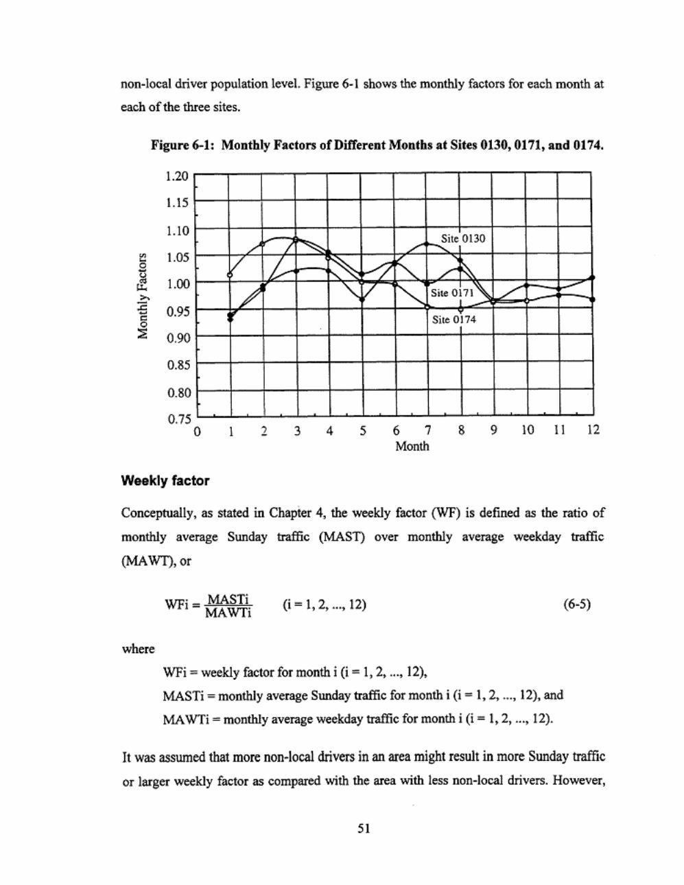
non-local driver population leveL Figure 6-1 shows the monthly factors for eacb month at
each of the three sites.
Figure 6-1: Monthly Factors of Different Monlbs at Sites 0130, 0171, and 0174.
~ ~
0 -<.>
!£ >. .c -c 0
::E
1.20
1.15
1.10
1.05
1.00
0.95
0.90
0.85
0.80
0.75 0
/ I ~ v t ~ ~ "
I 2 3 4
Site 0130
V/ ......... / ~
v f"._ Site 0:11'\. /
Site 0174
5 6 7 8 9 10 II 12 Month
Weekly factor
Conceptually, as stated in Chapter 4, the weekly factor (WF) is defined as the ratio of
monthly average Sunday traffic (MASl) over monthly average weekday traffic
(MAW!), or
where
WFl. = MASTi MAWTi
(i=l,2, ... ,12)
WFi =weekly factor for month i (i =I, 2, ... , 12),
MASTi = monthly average Sunday traffic for month i (i = I, 2, ... , 12), and
MA WTi - monthly average weekday traffic for month i (i = I, 2, .. . , 12).
(6-5)
It was assumed that more non-local drivers in an area might result in more Sunday traffic
or larger weekly factor as compared with the area with less non-local drivers. However,
51

some areas such as Orlando may attract non-local drivers during the whole week
including Sunday and weekdays in which case more non-local drivers may not
necessarily result in a larger weekly factor. Figure 6-2 presents weekly factors for each
month at the three sites.
Figure 6-2: Weekly Factors of Different Months at Sites 0130,0171, and 0174.
~ 0 u IZ ,., .:>< 8 ~
1.10
1.00
0.90
0.80
0.70
0.60
0.50
0.40
0.30 0
Daily factor
v v
I 2
/ ........ .
/
"
3 4 5
Site 0130
......... .
...... .......
"' / Site 0174-
/
Site 0171
6 7 8 9 10 I I 12 Month
The daily factor (DF) is defmed as the ratio of monthly average weekday afternoon non
peak traffic (I :00 pm - 2:00 pm, Monday, Tuesday, Wednesday, and Thursday only) to
monthly average weekday morning rush-hour traffic (7:00 am - 8:00 am, Monday,
Tuesday, Wednesday, and Thursday only), or
v· DF
. _ 11- 2pm ' - v· 17- Sam
(i = 1, 2, ... , 12) (6-6)
52

where
DFi ~daily factor for month i (i ~ I, 2, ... , 12),
Vi1_2pm =monthly average weekday afternoon non-peak traffic for month i (i = I,
2, ... , 12), and
Vi7_8am =monthly average weekday morning rush-hour traffic for month i (i = 1,
2, ... , 12).
Generally, morning rush-hour traffic consists of mostly commuters and regular user
traffic. However, during the afternoon non-peak time, the traffic has a h.igher proportion
of non-local driver traffic. Higher non-local driver population levels would result in
larger daily factors. The daily factor may be used as an indirect measure of non-local
driver population level. Figure 6-3 depicts daily factors for each month at the three sites.
Figure 6-3: Daily Factors of Different Months at Sites 0130, 0171, and 0174.
1.10
1.00
0.90
0.80
0.70
0.60
0.50
0.40
0.30 0
,/
I 2 3 4 5
53
.,... ......... Sice
00174
Sice ~B~.., Sice bm
6 7 8 9 10 II 12 Month

Correlation between monthly factor, weekly factor, and daily factor
To jointly use monthly factor, weekly factor, and daily factor to indirectly indicate non
local driver population levels, the three factors should not statistically correlate to each
other. Correlation analyses were performed in the study to confirm that there was no
statistical correlation between these factors. Table 6-1 presents R' values between
monthly factor, weekly factor, and daily factor. It can be seen that the correlation
coefficients between any pairs of factors were very small. This suggested all three factors
were independent from each other and could be used as independent variables in
regression analysis to develop an index indirectly representing non-local driver
population levels.
Table 6-1: Correlations Between Factors.
Factors R2
MF,WF 0.0153 MF,DF 0.0059 WF,DF 0.0166
Speed-Volume Models
Traffic data were collected from three sites including sites 0130, 0171, and 0174. As
stated in Chapter 3, the speed-volume curve can be represented by a linear model, or
Speed= a+ b x Volume (6-7)
where the parameter "a" is free-flow speed and the parameter "b" is affected by non-local
driver population level if other conditions are given. Table 6-2 presents the parameters
and corresponding R' values obtained from the data collected from the three sites. It can
be seen that some data were missing from the original database. This database was not
sufficient to include all data collected from each month and each lane. The results
presented in the rest of the Chapter were based on the data files that had sufficient volume
and speed data.
54
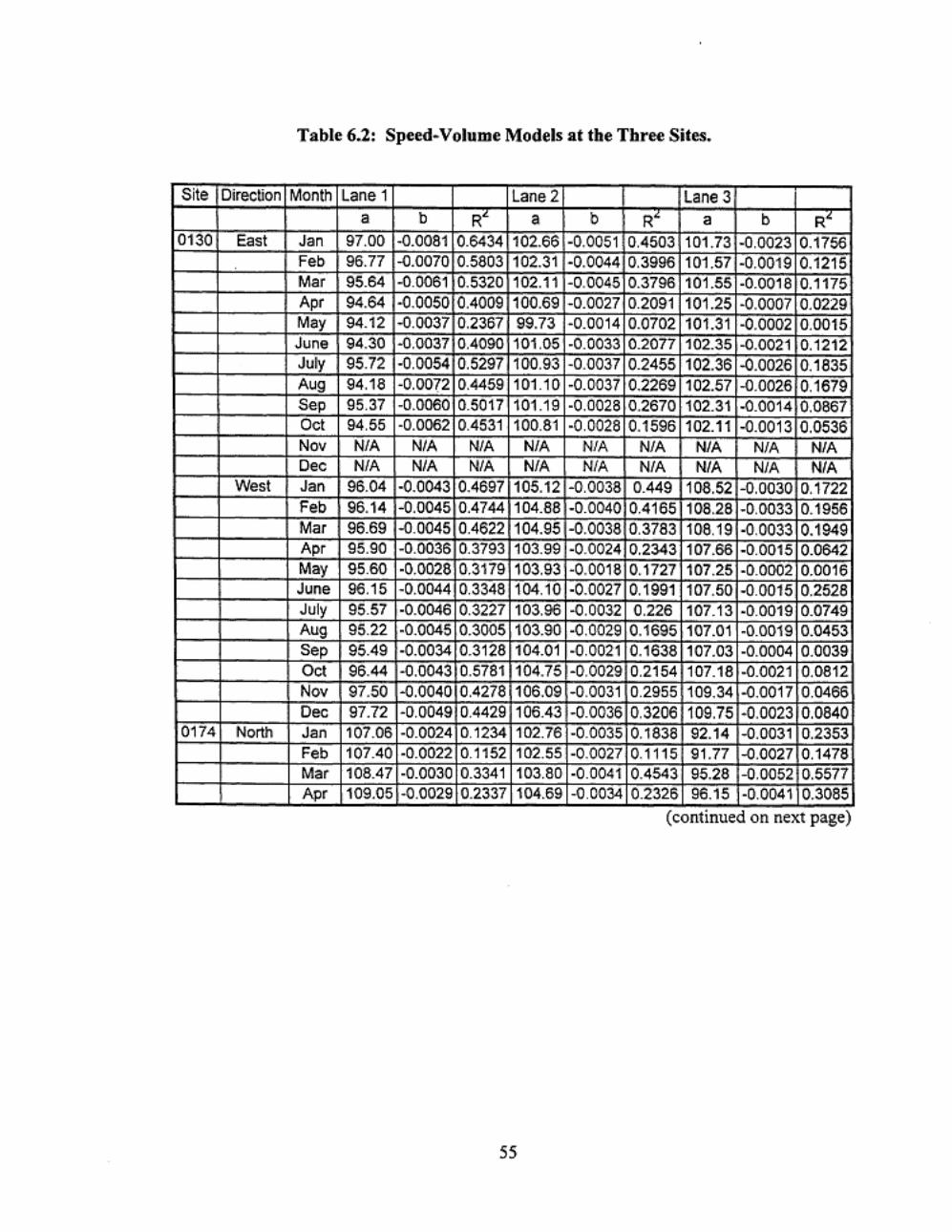
Table 6.2: Speed-Volume Models at tbe Three Sites.
Site Direction Month Lane 1 Lane 2 lane 3 a b R" a b R" a b R'
0130 East Jan 97.00 -0.0081 0.6434 102.66 -0.0051 0.4503 101.73 -0.0023 0.1756 Feb 96.77 -0.0070 0.5803 102.31 ·0.0044 0.3996 101 .57 -0.0019 0.1215 Mar 95.64 -0.0061 0.5320 102.11 -0.0045 0.3796 101.55 -0.0018 0.1175 Apr 94.64 -0.0050 0.4009 100.69 -0.0027 0.2091 101.25 -0.0007 0.0229 May 94.12 -0.0037 0.2367 99.73 -0.0014 0.0702 101.31 -0.0002 0.0015 June 94.30 -0.0037 0.4090 101.05 -0.0033 0.2077 102.35 -0 .0021 0.1212 July 95.72 -0.0054 0.5297 100.93 -0 .0037 0.2455 102.36 -0.0026 0.1835 Aug 94.18 -0.00(2 0.4459 101 .1 0 -0.0037 0.2269 102.57 -0.0026 0.1679 Sep 95.37 -0.0060 0.5017 101.19 -0.0028 0.2670 102.31 -0.0014 0.0867 Oct 94.55 -0.0062 0.4531 100.81 ·0.0028 0.1596 102.11 -0.0013 0.0536 Nov N/A N/A N/A N/A N/A N/A NIA N/A NIA Dec N/A N/A N/A N/A N/A N/A N/A N/A N/A
West Jan 96.04 -0.0043 0.4697 105.12 ·0.0038 0.449 108.52 -0.0030 0.1722 Feb 96.14 -0.0045 0.4744 104.88 -0.0040 0.4165 108.28 -0.0033 0.1956 Mar 96.69 -0.0045 0.4622 104.95 -0.0038 0.3783 108.19 -0.0033 0.1949 Apr 95.90 -0.0036 0.3793 103.99 -0.0024 0.2343 107.66 -0.0015 0.0642 May 95.60 -0.0028 0.3179 103.93 -0.0018 0.1727 107.25 -0.0002 0.0016 June 96.15 -0.0044 0.3348 104.10 ·0.0027 0.1991 107.50 -0.0015 0.2528 July 95.57 -0.0046 0.3227 103.96 ·0 .0032 0.226 107.13 -0.0019 0.0749 Aug 95.22 -0.0045 0.3005 103.90 -0.0029 0 .1695 107.01 -0.0019 0.0453 Sep 95.49 -0.0034 0.3128 104.01 -0.0021 0.1638 107.03 -0.0004 0.0039 Oct 96.44 -0.0043 0.5781 104.75 -0.0029 0.2154 107.18 -0.0021 0.0812 Nov 97.50 -0.0040 0.4278 106.09 -0.0031 0.2955 109.34 -0.0017 0.0466 Dec 97.72 ·0.0049 0.4429 106.43 -0.0036 0.3206 109.75 -0.0023 0.0840
0174 North Jan 107.06 -0.0024 0.1 234 102.76 -0.0035 0.1838 92.14 -0.0031 0.2353 Feb 107.40 -0.0022 0.1152 102.55 -0.0027 0.1115 91.77 -0.0027 0.1478 Mar 108.47 -0.0030 0.3341 103.80 -0.0041 0.4543 95.28 -0.0052 0.5577 Apr 109.05 -0.0029 0.2337 104.69 -0 .0034 0.2326 96.15 -0.0041 0.3085 .
(contmued on next page)
55

Table 6.2: Speed-Volume Models at tbe Three Sites (coDtinued).
Site Direction Month Lane 1 Lane2 Lane3 May 108.81 -0.0016 0.1126 104.86 -0.0022 0 .1 509 96.73 -0.0030 0.2255 June 108.45 -0.0025 0.1 694 104.49 ·0.0032 0.2188 97.19 -0.0046 0.4198 July 108.59 -0.0018 0.0837 104.50 -0.0025 0.1330 96.97 -0.0035 0.2749 Aug 107.72 -0.0019 0.0545 103.97 -0.0025 0.0867 96.55 -0.0035 0.2114 Sep 108.60 -0.0016 0.0594 104.74 -0.0021 0.0842 96.73 -0.0027 0.1209 Oct 107.44 -0.0017 0.0462 104.00 -0.0027 0.0949 96.07 -0.0031 0.1344 Nov 106.61 -0.0076 0.7482 103.90 -0.0040 0.4976 114.13 -0.0031 0.4078 Dec 106.39 -0.0077 0.7178 98.25 -0.0040 0.3098 114.70 -0.0032 0.3539
0174 South Jan 110.37 -0.0050 0.3661 110.76 -0.0077 0.5729 96.96 -0.0057 0.3574 Feb 110.29 -0.0040 0.2469 110.84 -0.0071 0.5920 96.48 -0.0046 0.2830 Mar 101.43 -0.0053 0.1 496 109.45 -0.0062 0.4019 105.97 -0.0045 0.1296 Apr 99.67 ·0.0067 0.6794 109.31 -0.0059 0.6843 110.93 -0.0042 0.3075 May NIA NIA NIA NIA NIA NIA NIA N/A N/A June NIA N/A NIA N/A NIA NIA NIA N/A N/A July NIA N/A- NIA N/A N/A NIA NIA N/A N/A Aug 98.25 -0.0050 0.3098 107.90 -0.0048 0.3220 109.09 ·0.0028 0.1141 Sep 97.94 -0.0042 0.2576 109.10 -0.0052 0.3226 108.85 -0.0022 0.1105 Oct 98.22 ·0.0041 0.2297 NIA N/A N/A 108.75 -0.0017 0 .0532 Nov 103.77 ·0.0070 0.4099 112.43 -0.0050 0 .1873 116.65 -0.0056 0.6330 Dec 105.89 -0.0074 0.4636 110.64 -0.0062 0 .4041 116.30 -0.0055 0 .4003
0171 North Jan 101.31 -0.005 0.5274 102.53 -0.0029 0.4015 NIA NIA N/A Feb 101.62 -0.0051 0 .5197 102.74 -0 .0029 0.3769 NIA NIA N/A Mar 102.79 -0.0063 0.5785 103.78 -0.0037 0.4574 NIA NIA N/A Apr 103.03 ·0.006 0.5239 104.29 -0.0038 0.4535 N/A N/A N/A May 102.76 -0.0056 0.5418 104.1 -0.0035 0.5007 NIA N/A N/A June 101.4 -0.005 0.4761 103.22 -0.0031 0.4469 N/A NIA N/A July 102.13 -0.005 0.4417 103.86 -0.0032 0.3976 NIA N/A N/A Aug 101.92 -0.0056 0.44 103.77 -0.0037 0.4019 N/A NIA NIA Sep 101.41 -0.0053 0.4322 103.79 -0.0039 0.4193 NIA NIA N/A Oct 100.77 -0.0046 0.3544 103.29 -0 .0033 0.3011 NIA N/A N/A Nov 102.05 -0.0055 0 .5377 103.43 -0 .0033 0.4240 NIA N/A N/A Dec 102.17 -0.0050 0.4763 103.44 -0.0029 0.3480 N/A N/A N/A
South Jan 115.20 -0.0130 0.8846 103.40 -0.0029 0.3470 NIA NIA N/A Feb 114.59 -0.0127 0.8619 103.74 -0.0028 0.3215 N/A NIA NIA
Mar 115.01 -0.0129 0.8374 103.60 -0.0028 0 .2921 NIA NIA N/A Apr 114.30 -0.0124 0.7970 103.78 -0.0030 0.2438 NIA NIA N/A
May 112.66 -0.0108 0.7731 103.96 -0.0027 0.2722 N/A NIA NIA June 114.07 -0.0118 0.7956 102.91 -0.0022 0.1916 N/A NIA NIA
July 114.65 -0 .0117 0.7451 103.03 -0.0023 0.1661 NIA NIA N/A Aug 114.59 -0.0123 0.7594 102.62 ·0.0026 0.1982 NIA NIA NIA
Sep 114.41 -0.0128 0.7878 103.21 -0 .0031 0 .2688 NIA N/A N/A
Oct 116.85 ·0.0143 0.7593 102.96 -0.0031 0.2331 NIA NIA NIA
Nov 118.85 ·0.0145 0.7711 104.10 -0.0032 0.3010 N/A N/A N/A
Dec 111.57 -0,0105 0.74401103.87 -0.0250 0.2109 NIA NIA N/A
56

Development of an Index
Model specifications
The monthly factor, weekly factor, and daily factor are related to non-local driver
population level. To indirectly represent the non-local driver population level, an index
was developed in the study. Several formats of the index were evaluated in the study.
Specifications of the index are presented in Table 6-3. To practically use the index, the
index format should be simple and easy to be implemented. The linear combination of
these factors to form the index would be a practically feasible way. Determination of the
final format would depend on the parameter sign of each factor and also the R' value of
each format.
Table 6-3: Index Model Specifications.
Format Dependent Variable
Independent Variables Index Model Formats
I b MF. WF. DF b=kO+ kl x MF+k2 x WK+ k3 xDF
2 b MF. WF b=kO +kl X MF +k2 X WK
3 b MF,DF b=kO+kl xMF+k3xDF
4 b WF.DF b = kO + k2 X WK + k3 " DF
Index calibration
The index should reflect the relative levels of non-local driver population. One reasonable
way to calibrate the index parameters (kO, kl, k2, and k3) was to correlate the index with
the parameter "b" shown in Equation 6· 7 because the parameter "b" reflec.ts the relative
levels of non-local driver population in the traffic streams. A linear regression analysis
was performed to calculate the parameters kO, kl, k2, and k3. The analysis was based on
the data shown in Tables 4-3 and 6-2, and results are presented in Table 6-4.
Conceptually, a reasonable index format should have negative signs for the parameters
associated with the factors because as the factors get larger, more non-local drivers may
exist in the traffic stream, resulting in smaller "b" value. This means that the parameters
57
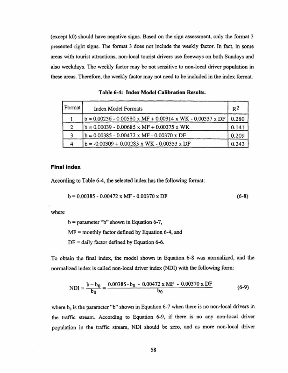
(except kO) should have negative signs. Based on the sign assessment, only the format 3
presented right signs. The format 3 does not include the weekly factor. In fact, in some
areas with tourist attractions, non-local tourist drivers use freeways on both Sundays and
also weekdays. The weekly factor may be not sensitive to non-local driver population in
these areas. Therefore, the weekly factor may not need to be included in the index format.
Table 6-4: Index Model Calibration Results.
Format Index Model Formats
I b = 0.00236- 0.00580 X MF + 0.00314 X WK - 0.00337 X DF
2 b = 0.00039 - 0.00685 X MF + 0.00375 X WK
3 b = 0.00385 - 0.004 72 x MF- 0.00370 x OF
4 b = -0.00309 + 0.00283 x WK - 0.00353 x OF
Final Index
According to Table 6-4, the selected index has the following format:
where
b = 0.00385 - 0.00472 x MF- 0.00370 x OF
b = parameter "b" shown in Equation 6-7,
MF =monthly factor defined by Equation 6-4, and
OF= daily factor defined by Equation 6-6.
R2
0.280
0.141
0.209
0.243
(6-8)
To obtain the fmal index, the model shown in Equation 6-8 was normalized, and the
normalized index is called non-local driver index (NDI) with the following form:
b-b0 0.00385-bo- 0.00472xMF- 0.00370xDF (6
_9)
NDI= bo = bo
where b0 is the parameter "b" shown in Equation 6-7 when there is no non-local drivers in
the traffic. stream. According to Equation 6-9, if there is no any non-local driver
population in the traffic stream, NDI should be zero, and as more non-local driver
58
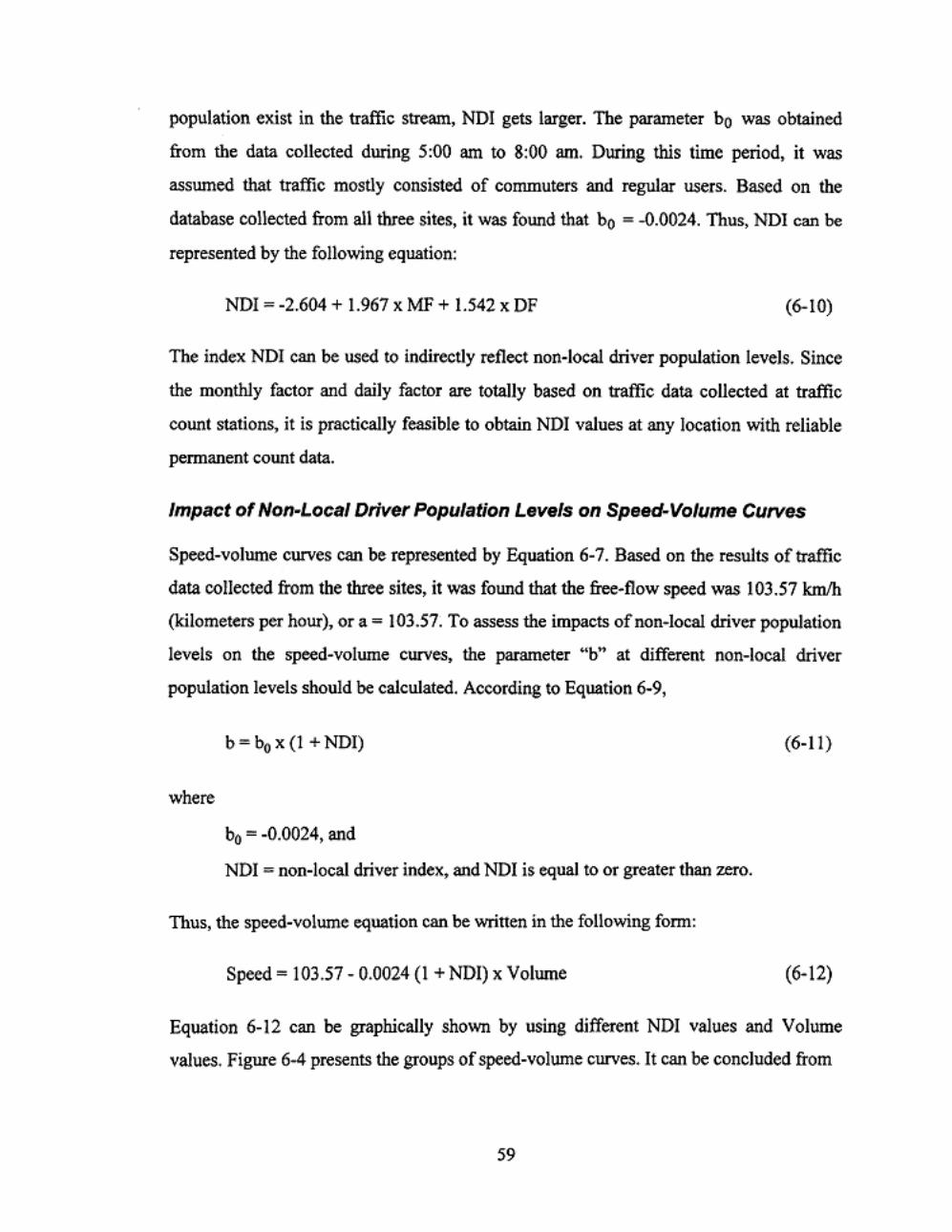
population exist in the traffic stream, NDI gets larger. The parameter bo was obtained
from the data collected during 5:00 am to 8:00 am. During this time period, it was
assumed that traffic mostly consisted of commuters and regular users. Based on the
database collected from all three sites, it was found that bo = -0.0024. Thus, NDI can be
represented by the following equation:
NDI ~ -2.604 + 1.967 X MF + 1.542 X DF (6-10)
The index ND! can be used to indirectly reflect non-local driver population levels. Since
the monthly factor and daily factor are totally based on traffic data collected at traffic
count stations, it is practically feasible to obtain NDI values at any location with reliable
permanent count data.
Impact of Non-Local Driver Population Levels on Speed-Volume Curves
Speed-volume curves can be represented by Equation 6-7. Based on the results of traffic
data collected from the three sites, it was found that the free-flow speed was I 03.57 kmlh
(kilometers per hour), or a= !03.57. To assess the impacts of non-local driver population
levels on the speed-volume curves, the parameter "b" at different non-local driver
population levels should be calculated. According to Equation 6-9,
b = b0 x (I + NDI) (6-11)
where
b0 = -0.0024, and
NDI = non-local driver index, and NDI is equal to or greater than zero.
Thus, the speed-volume equation can be written in the following form:
Speed= 103.57 • 0.0024 (1 + NDI) x Volume (6-12)
Equation 6-12 can be graphically shown by using different NDI values and Volume
values. Figure 6-4 presents the groups of speed-volume curves. It can be concluded from
59

this figure that as NDI increases (more non-local driver population in the traffic stream),
speed decreases if the same volume is to be maintained.
Figure 6-4: Impact of Non-L<Ical Driver Population on Average Operating Speed.
105r-.,-.~~~~ro~-r~~~~~~~ ~
] 100 1-t--r-+: ~
1 ~ 95~~-+~~~4-+-~
"" c
·~ 90 H-+-t-+-HH-++-+-~--1-....j....::: 8. 0
200GB D I~ ID IG 1~18002~
Volume (pcphpl)
Estimate of Driver Population Factors
NDI=Q NDI=0.2 NDI=0.4 NDI=Q.6
NDI=Q.S
" NDI=I.O NDI=1.2
• NDI=l.4 NDI=1.6
• NDI=I.8 a NDI=2.0
NDI=2.2 NDI=2.4
• NDI=2.6
It can be understood that as non-local driver population level increases, traffic volume or
flow rate is going to decrease if the same density is to be maintained. In this study, three
density lines which defme LOS B, C, and D, respectively were used to evaluate the
capacity reductions at different levels of non-local driver population (different NDI
values). Figure 6-5 presents the density line of LOS C. For the given density line, traffic
flow rates or volumes corresponding to different NDI values can be obtained by checking
the corresponding volume data at the intersects of the density line and the speed-volume
curves. Table 6-5 lists the volume data corresponding to different NDI values at LOS B,
C, and D. Based on this table, driver population adjustment factors, fP, can be estimated.
For example, to estimate fP value when NDI ~ 1.2 with given condition of LOS D, the
volume data at NDI = 0.0 and NDI ~ 1.2 should be checked. In this case, volume ~ 1963
for NDI = 0.0 and volume= 1862 for NDI = 1.2. Thus,
f. - 1862 - 0949 p- 1963 - . (NDI = 1.2)
60

Figure 6.5: Density Line for LOS C (14.92 pclkmlln).
II
-• •
80 l±t±t±ttt±±tt];~;!LJ 0 ~ G 8 B 1~1~1G 1~1BWOO
D
Volume (pcphpl)
Table 6-5: Maximum Service Volumes (pcphpl) for LOS B, C, and D aud Different NDI Values.
NDI LEVEL OF SERVICE (LOS)
LOSB LOSC LOSD
0.0 1005 1492 1963 0.2 1000 1482 1947 0.4 996 1472 1929 0.6 991 1462 1911 0.8 987 1452 1895 1.0 982 1442 1880 1.2 978 1432 1862 1.4 973 1423 18-17 1.6 969 1413 1831 1.8 965 1404 1816 2.0 96 1 1395 1800 2.2 956 1386 l i 87 2.4 952 1377 l'i71 2.6 948 1368 !'57
61
NDI=O NDI=0.2 NDI=0.4 NDI=0.6 ND1=0.8 NDI=l.O NDI=l.2 NDI=i.4 NDI=1.6 NDI=l.S NDI=2.0 NDI=2.2 NDI=2.4 NDJ=2.6
LOSC
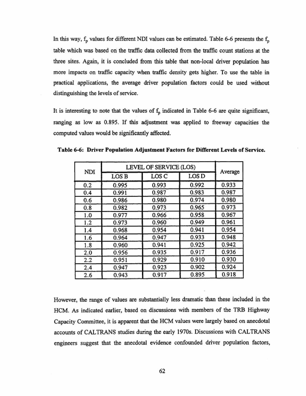
In this way, fp values for different NDI values can be estimated. Table 6-6 presents the t;, table which was based ori the traffic data coUected from the traffic count stations at the
three sites. Again, it is concluded from this table that non-local driver population has
more impacts on traffic capacity when traffic density gets higher. To use the table in
practical applications, the average driver population factors could be used without
distinguishing the levels of service.
It is interesting to note that the values of fp indicated in Table 6-6 are quite significant,
ranging as low as 0.895. If this adjustment was applied to freeway capacities the
computed values would be significantly affected.
Table 6-6: Driver Population Adjustment Factors for Different Levels of Service.
NDI LEVEL OF SERVICE (LOS)
Average LOSB LOSC LOSD
0.2 0.995 0.993 0.992 0.933 0.4 0.991 0.987 0.983 0.987 0.6 0.986 0.980 0.974 0.980 0.8 0.982 0.973 0.965 0.973 1.0 0.977 0.966 0.958 0.967 1.2 0.973 0.960 0.949 0.961 1.4 0.968 0.954 0.941 0.954 1.6 0.964 0.947 0.933 0.948
1.8 0.960 0.941 0.925 0.942 2.0 0.956 0.935 0.917 0.936 2.2 0.951 0.929 0.910 0.930 2.4 0.947 0.923 0.902 0.924 2.6 0.943 0.917 0.895 0.918
However, the range of values are substantially less dramatic than these included in the
HCM. As indicated earlier, based on discussions with members of the TRB Highway
Capacity Committee, it is apparent that the HCM values were largely based on anecdotal
accounts of CAL TRANS studies during the early 1970s. Discussions with CAL TRANS
engineers suggest that the anecdotal evidence confounded driver population factors,
62
vehicle classification factors, and perhaps highway grade factors to read a factor as low as
0.75. If our estimates of fp were observed, in conjunction with high levels of heavy duty
vehicles and lower design standards, a combined factor of0.75 is within reason.
Discussion
The driver population adjustment factor table obtained from this study and presented in
this chapter is totally based on traffic data collected from traffic count stations. FOOT has
full accessibility to obtain traffic data from their traffic count stations. This table has
more practical potentials to be used by transportation practitioners as compared with the
driver population adjustment factor table presented in Chapter 5.
To use this driver population adjustment factor table, the monthly factor and weekly
factor for a particular location and during a particular time period should be obtained.
FDOT can use the traffic data collected from the traffic count station at the particular site
to calculate the monthly factor and weekly factor according to the definitions of the two
factors. After obtaining the monthly factor and weekly factor, the practitioner can use
Equation 6-10 to calculate the NDI value. Finally, the £;, value can be checked by using
Table 6-6.
Traffic data collected from the three sites were not I 00 percent comprehensive. Because
of roadway construction or some other unusual activities occurred, traffic data in some
months were not included in the database obtained from FDOT. Results based on such
incomplete database may not fully represent the practical situation. To develop better
models based on a completed database, field data collection should be better controlled,
and a new database would be necessary. However, the methodologies used in this study
can be fully applied to obtain better models.
63

CHAPTER 7: SUMMARIES, CONCLUSIONS, AND RECOMMENDATIONS
Summary
This study was performed to develop a driver population factor table to be used by
transportation practitioners in transportation planning and design. The main objectives
were:
I. Conduct literature and information search on past studies related to the subject
area. The main information resources included information databases searched
through computer network, technical papers reviewed in the study, expert
comments obtained through telephone conversations;
2. Assess methodologies which could be used to evaluate the impacts of non-local
driver population on roadway capacities;
3. Design experiments for the data collection of non-local driver population
information and capacity reduction due to non-local driver population;
4. Assess study data resources and collect data to be used in the study. The data
sources used in this study to develop driver population adjustment factor tables
included (I) tourist survey database developed by the Office of Tourism Research,
Bureau of Economic Analysis of the Florida Department of Commerce and (2)
traffic database developed by FOOT to include traffic data collected from FOOT's
traffic count stations;
5. Develop indices used to indirectly represent non-local driver population levels.
The indices developed through this objective were based on the data sources from
the Office ofTourism Research and FDOT; and
64

6. Evaluate the impacts of non-local driver population on freeway capacity and
develop driver population adjustment factor tables based on tourist survey
database and traffic database.
This study was divided into two phases. Phase I consisted of the study objectives I to 4.
Phase I results were summarized in an interim report. Phase ll focused on study
objectives 5 and 6 . This report summarizes the study results related to objectives 5 and 6.
In this study, two main methods of developing driver population adjustments were
attempted. This first way was to use data to estimate non-local driver population levels
and corresponding capacity reductions caused by non-local driver population. Based on
the estimations of non-local driver population levels and capacity reductions, a driver
population adjustment factor table was developed and presented in this report.
In the second way, the concept of monthly factor, weekly factor, and daily factor was
developed. These factors were considered as the candidates to indirectly reflect non-local
driver population levels. An index called non-local driver index (NDI) was developed to
linearly combine the monthly factor and daily factor. Based on the NDI model
specifications and assessment, the monthly factor and daily factor were selected and
included in the NDI model. Similar to the first way, capacity reductions corresponding to
different NDI values were estimated. Thus, a driver population adjustment factor table
was developed and presented in the report.
Conclusions
The population factor is an important adjustment factor in freeway capacity analyses.
Unfortunately, the HCM provides little guidance on how to choose appropriate fp values.
The fP values recommended in the HCM need to be verified. Past studies were not able to
supply adequate solutions to deal with this problem.
Unlike roadway geometric and heavy vehicle percentage, it is much more difficult to
measure driver populations than other external capacity factors such as lane widths and
65
clearances (fw). and vehicle types (fi!V). Traditional direct measurements such as roadside
interviews and license plate surveys are practically not feasible for driver population
estimation.
There are many elements and considerations associated with driver populations, including
trip purpose, trip origin and destination, familiarity, driver age, etc. In Florida, the
dominate element is the familiarity with highway facilities. In this study, non-local driver
population levels were used to represent different driver populations in freeway traffic in
Florida.
Tourist survey data and traffic volume variations are the two indirect measurements
which are capable of providing reasonable driver population estimation. Tourist survey
data maintained by the Office of Tourism Research could supply acceptable driver
population estimation for freeway sections with adjacent tourist attractions. Monthly
factors and daily factors computed according to traffic volume variations could provide
reasonable information about driver populations for any freeway sections in Florida.
Freeway traffic data are collected continuously by the Florida Department of
Transportation. Transportation engineers could have easy access to historical freeway
traffic data.
Freeway capacity reductions could be estimated from the linear speed-volume models.
High traffic volumes are essential in the speed-volume modeling process. It is difficult to
develop speed-volume models under low traffic volumes. In the speed-volume models,
mixed traffic volumes were transferred to passenger cars to take account of capacity
reductions caused by heavy vehicles. Therefore, different speed-volume lines could be
observed if there is any capacity reduction caused by different driver populations. Density
lines were used to compute actual fP values.
Two driver population adjustment factor tables were developed through this study and
presented in this report. The first table was obtained based on the tourist survey database.
To use the table, a driver index (DI) should be obtained for a particular area. Dl values
66

can be calculated from the tourist survey database maintained by the Office of Tourism
Research. The Office of Tourism annually updates its tourist survey database. The second
table was obtained based on the data collected from FOOT traffic count stations. To use
the table, the monthly factor and daily factor should be calculated from the database
maintained by FOOT. According to the monthly factor and daily factor, an index called
non-local driver index (NDI) can be calculated. With the given NDI value, a driver
population adjustment factor can be checked from the table. FOOT has full accessibility
to the FDOT database, it may be more practically feasible for FOOT to use the second
table as compared with the first table.
Indirect measurements of non-local driver population levels such as the indices DI and
NOI are practically useful to transportation practitioners. It is relatively easier for
transportation practitioners to obtain the indirect measurements such as DI and NDI than
the absolute percentage of non-local driver population in the traffic streams. In fact, when
a transportation practitioner is going to estimate the driver population adjustment factor
for planning or design purposes, this practitioner may not be able to know the information
on the absolute percentage of non-local driver population. However, this practitioner is
able to know the monthly factor and daily factor for the particular location and the
particular time period. Therefore, the indirect measurements developed in this study will
be practically applicable.
The models developed through this study were based on 1995 databases. As stated in
previously chapters, these databases were not complete. Some data from some locations
and collected in some months were not included in the databases. Consequently, the
models may not be as perfect as they should be because of the incomplete databases.
However, the modeling procedures developed through this study provide a practically
feasible way to develop driver population adjustment factor tables. In future, if new data
are collected, better models can be obtained by using the same modeling procedures.
As noted in Tables 5-3 and 6-6, based on our limited data sample, t;, values as low as .85
to .9 are justified in areas with high non-local driver populations.
67

Recommendations for Future Research
The results obtained through this study and presented in this report can only be
considered preliminary fmdings. While the results are very promising, they are based on a
limited sample of sites. Their statistical robustness could be increased by additional
replications. During the course of this project, efforts have been underway that are
dramatically improving the reliability of FOOT's permanent count traffic data.
To reliably and efficiently use the results obtained from the study, a follow-up new
research study is strongly recommended. In the new study, more FDOT traffic count
stations should be used to collect better and more complete longitudinal traffic data in
terms ofhigb traffic volume, shorter time interval (such as IS-minute interval), consistent
12-month-data-collection period, no construction activities around the station sites, and
more widely distributed locations.
An additional area suggested for future research is to examine the influence of driver
population factor in more complex freeway sections, particularly weaving sections. It
would be expected that the influence of non-familiar drivers would be more severe in
complex weaving sections than on basic freeway sections.
68
REFERENCES
Brilon W. and M. Ponzlet, "Variability of Speed-Flow Relationships on German
Autobahns," Transportation Research Record No. 1555, 1997, pp. 91-97.
FHWA, Highway Statistics 1994, FHWA-PL-95-042, Federal Highway Administration,
Washington, D.C, 1994.
FHW A, Passenger Car Equivalents for Rural Highways, FHW AIRD-821132, Federal
Highway Administration, Washington, D. C., 1982.
FOTR, Florida Visitor Study, Florida Office of Tourism Research, Florida Department of
Commerce, Tallahassee, Florida, 1995.
Highway Capacity Manual, Transportation Research Boan:l, Special Repon 209, 1994.
HPMS Universe Totals, Florida Department of Transportation, Tallahassee, Florida,
1994.
May, A. D., Traffic Flaw Fundamentals, Prentice-Hall, Inc., Englewood Cliffs, New
Jersey, 1990.
Minderhoud, M. M., "An Assessment of Roadway Capacity Estimation Methods,"
presented at the 76th Annual Meeting of Transportation Research Board, Washington,
D. C., 1997.
NCHRP 3-45, Speed-Flow Relationships for Basic Freeway SegmentS, Transportation
Research Board, May, 1995.
OECD, Traffic Capacity of Major Routes, Road Transportation Research, Organization
for Economic Co-operation and Development, Paris, France, July 1983.
69
Sharma, S. C. L , et a!, "Driver Population Factor in the New Highway Capacity
Manual," Journal a/Transportation Engineering, Vol. 113, No.5, 1987, pp. 575-579.
Sharma, S. C. L., et a!, "Road Classification According to Driver Population,"
Transportation Research Record No. 1090, 1986, pp. 61-69.
Sharma, S. C. L., et al, "Seasonal Traffic Counts for a Precise Estimation of AADT," ITE
Journal, Vol. 64, No.9, 1994, pp. 21-28.
UPF, Florida Statistical Abstract. University Press of Florida, Gainesville, Florida, 1995.
70