Embed Size (px)
Citation preview
i
Academic Year 2016-17
DRIP IRRIGATION TECHNOLOGY IN
HARD ROCK FARMING AREAS.
TESTING JEVONS PARADOX IN
KARNATAKA, INDIA
Kabbur, Rashmi
Promotor: Prof. Dr.ir. Stijn Speelman
Thesis submitted in the partial fulfilment of the requirement for the joint academic degree programme
of International Master in Rural Development (IMRD) from Ghent University (Belgium), Agro-campus
Ouest (France), Humboldt University of Berlin (Germany), Slovak University of Agriculture in Nitra
(Slovakia) and University of Pisa (Italy) in collaboration with Can Tho University (Vietnam), China
Agricultural University (China), Escuela Superior Politecnica del Litoral (Ecuador), Nanjing Agricultural
University (China), University of Agricultural Sciences Bengaluru (India), University of Pretoria (South
Africa).

ii
This thesis was elaborated and defended at Ghent University, Faculty of Bioscience Engineering, Department of Agricultural Economics, within the
framework of the European Erasmus Mundus Joint Master Degree “International Master of Science in Rural Development" (Course N° 2015-1700 / 001 - 001)
Certification
It is a unpublished M.Sc. report and is not prepared for further distribution. The author and the promoter give the permission to use this thesis available for consultation and to copy parts of it for personal use. Every other use is
subjected to the copyright laws; more specifically the source must be extensively specified when using results from this thesis.
The Promoter(s) The Author
Prof. Dr. ir. Stijn Speelman Rashmi Shivamurthy Kabbur
(Name(s) and Signature (s)) (Name and Signature)
Thesis online access release
I hereby authorize the IMRD secretariat to make this thesis available online on the IMRD website.
The Author
Rashmi Shivamurthy Kabbur
(Name and Signature)
iii
Acknowledgement
I place my deep sense of gratitude with at most sincerity and heartfelt respect to
my promoter Prof. Dr. ir. Stijn Speelman. For his valuable teaching, guidelines
and cooperation throughout my study programme. My special thanks to my
tutor Gonzalo Gabriel Villa-Cox for his consistence assistance and
encouragement at every stage of my research work. I am grateful to my friends
Preetham, Raghavendra, Amurutha, Sandhya, Tim, Khin, Lavanya, Deepu
Swamy, Vijay Kumar, Goldi, Sathish Kumar, Veerabhadrappa and not only for
their help during data collection but also for the moral support. My sincere
gratitude to farmer Prasad and his family for their hospitality and assistance
during my research survey. Without their friendly support and generosity my
research work would not have been completed. My study would not be
complete without thanks to my family for their unconditional support during
this programme.
At last but not least, I also want to dedicate my gratitude to the sampled farmers
of Chikkaballapura district for sharing their valuable time and relevant
information required by this study.
iv
Abstract
Technology inventions are often increases resource use efficiency. However, the increased
resource use efficiency not always leads to resource conservation. It may open a way to raise
resource consumption due to reduced cost of production. This study aims to test Jevons
paradox in drip irrigation technology of hard rock areas of Karnataka, India. Chikkaballapura
district of Karnataka was chosen as study area. Farmers were chosen by purposive random
sampling. Data was collected from 109 drip irrigated farmers and 76 flood irrigated farmers
with structured questionnaire through face to face interview. For well failure intensity
between drip and flood irrigated farmers is assessed by negative binomial distribution. The
results indicated probability of well failure is 0.43 under drip irrigation against 0.31 in flood
situation. In addition, for every 100 drilling efforts, there were 43 and 31 failures in drip and
flood irrigation respectively. Secondly, Jevons paradox in drip irrigation is analysed by
propensity score matching. The probit model depicts that loan amount, average power of
pump used to lift groundwater affects significantly on drip adoption at 5 percent and distance
between borewell to the nearest water source, isolation distance between two borewell and
caste influences drip implementation significantly at 10 percent. The mean groundwater use
by drip farmers is 6.71, 12.66 and 12.85 acre-inch significantly less than flood irrigated
farmers by radius, kernel and nearest neighbour matching methods respectively. Therefore,
from the study results concludes that drip technology contributing to reduce groundwater use
and there was no rebound or Jevons paradox in the case drip technology of irrigation in hard
rock areas of Karnataka, India.

v
Contents
1 Introduction ………………………………………………………………………………. 1
1.1 Background…………………………………………………………………..………. 1
1.2 Introduction of drip Technology…………………………………………..….……… 2
1.3 Jevons paradox and its relevance to the study………………...……………..…….......3
1.4 Problem statement…………………………………………………….……..…….......5
1.5 Research gap …………………………………………...…………………..…….…...6
1.6 Research objectives ……………………………………………………….…..……....7
1.7 Limitation of the study …………………………………………………….…..……...7
2. Review of Literature ……..………………………………………………………..…….. 9
2.1 Groundwater exploitation and well failure in India ……………………………………... 9
2.1.1 Groundwater status before green revolution in India (before 1960s)……………….. 9
2.1.2 Groundwater status after green revolution in India ……………………………........10
2 .1.3 Groundwater status after 2000s onwards …………………………………………. 13
2.1.4 Extent of over-exploitation of groundwater and its consequences in India ……….. 14
2.2 Probability of well failure in India …………………………………………………….. 16
2.3 Emergence of water saving technologies in India ………………………………….…... 17
2.3.1 Importance of water saving technologies in India ……………………………..….. 17
2.3.2 Water saving technologies adopted in India ………………………………….….... 17
2.3.3 Emergence of micro-irrigation technology in India ……………………………..... 18
2.3.4 Factors determine drip irrigation adoption in India ………………………….…..... 19
2.3.5 Drip irrigation method as a water saving technology …………………………...… 20
2.4 Jevons Paradox in technology innovation and its relevance to drip irrigation ………..... 21
3. Methodology ………………………………………………………………..………..…. 23
3.1 Description of the study area ………………………………….………………...….…. 23
3.1.1 Agriculture profile of Karnataka state in India ……………..…………...……..… 23
3.1.2 Groundwater status and it’s exploitation in Karnataka …………...……………… 24
3.1.3 Agriculture profile of Chikkaballapura district of Karnataka, India …….……….. 25
3.1.4 Groundwater use in Chikkaballapura district of Karnataka ………………….…... 27
3.2 Sampling procedure ……………………………………………………………..……… 27
3.3 Analytical tools employed ………………………………………………….…….…….. 28
3.3.1 Negative binominal distribution ……………………………………………..….... 29
3.3.2 Propensity Score Matching …………………………………………...….………. 29
vi
3.2.2.1 Measurement of groundwater used in conventional irrigation system ….... 33
3.2.2.2 Measurements of groundwater used in drip irrigation system …….….….. 33
4. Results and Discussion …………………………………………………..……………... 35
4.1 Socio-economic features of sample farmers in the study area ………………..………... 35
4.2 Cropping pattern of the study area …………………………………………………..…. 38
4.3 Bore well failure and its reasons in the study area ……………………………………... 39
4.3.1 General profile of bore well irrigation in the study area, 2015-16 ………...….…. 39
4.3.2 Probability of bore well failure in the study area …………………………....…... 41
4.3.3 Reasons for borewell failure in the study area …………………………...…..….. 44
4.4 Testing of Jevons paradox in drip technology of irrigation in the study area ………….. 45
4.4.1 Estimation of probit model …................................................................................. 45
4.4.2 Propensity scores and average treatment estimation ………………….…...…….. 48
5. Conclusion and Recommendation ……………………………………………….……. 52
5.1 Introduction ……………………………………………….…………….…………….... 52
5.2 Major findings of the study ……………………….…………………….……………… 53
5.3 Recommendations ……………………………………….………………………………54
6. References ……………………………………………………………………...……….. 56
A Appendices ……………………………………………………………………………… 66
A.1 Photos of drip and flood irrigation method ………………………………………….… 66
A.1a Drip irrigation method ………………………………………………….………… 66
A.1b Flood irrigation method ……………………………………………………………67
A.2 Questionnaire used for the research data collection …..………………………..……… 68
A.3 Pictures from data collection ……………………………………………………….….. 79

vii
List of Tables
Table 1: Annual compound growth rate of net irrigated area in India (%)…………………. 12
Table 2: Comparative status of over-exploitation of groundwater in India from 1995 to
2011…………………………………………………………………………………………..15
Table 3: Description of independent variables used for probit analysis ……..…………….. 31
Table 4: Social characteristics of farmers following drip and flood irrigation in the study area,
2015-16……..………………………………………………………………………………. 36
Table 5: Economic characteristics of drip and flood irrigated farmers in the study area, 2015-
16……………………………………………………………………………………………..37
Table 6: Irrigation Intensity of the farmers following drip and flood irrigation in the study
area …………………………………………………………………………………..……... 39
Table 7: Borewell profile of the study area…………………………………………………. 40
Table 8: Probability of well success and failure in drip and flood irrigated farmers in the
study area…………………………………………………………………………….……… 43
Table 9: Reasons for borewell failure in the study area in 2015-16…………..….………… 44
Table 10: Estimates of endogenous variable with instrumental and other independent
variables of drip adoption in the study area……………………………………...…….…… 46
Table 11: Estimates of probit regression on drip irrigation adoption in the study area……...47
Table 12: Blocks/Cells for Treated and Control Groups to check balancing property
…….………………………………………………………………………………………... 48
Table13: Average treatment effect based on different matching method …………………...50

viii
List of Figures
Figure1: Percent share of irrigation to the total water used in selected countries, 1995…..... 11
Figure 2: Net irrigated area (000’ hectares) over the years in India………………………… 11
Figure 3: Percent share of different irrigation source to total net irrigated area, 1960-61, 2000-
01 and 2012-13 ………………………………………………………...…………………… 13
Figure 4: Comparative water use efficiency between micro and surface irrigation …...…… 18
Figure 5: Share of different sources to net irrigated area (%) between 2001-02 and 2010-11 in
Karnataka ………………………………………………………………………..…………. 24
Figure 6: Map showing study area in Karnataka state of India ……………..………….…... 26
Figure 7: Cropping pattern of Chikkaballapura district 2012-13, Karnataka………………..27
Figure 8: Proportion of farmers share based on farm size, Chikkaballapura ………………. 28
Figure 9: Cropping pattern of drip and flood irrigated farmers in the study region, 2015-16
……………………………………………………………………………………..…..……. 38
Figure 10: Frequency distribution of well failure to get a success among farmers following
drip and flood irrigation in the study area…………………………………………………... 41
Figure 11: Difference in well failure occurrence between drip and flood irrigation condition
of the study area ………………………………………………………………………….… 42
Figure 12: Probability of well success in the study area ……………….……………………43
Figure 13: Matching pattern between farmers practicing drip (treated) and flood (control)
irrigation in the study area ……………………………………………..…………………... 49

ix
List of Abbreviations
BCM – Billion Cubic Meters
CGWB – Central Ground Water Board
CIA – Central Intelligence Agency
CSO – Central Statistical Organization
DSAL – Digital South Asia Library
FAO – Food and Agriculture Organization
GDP – Gross Domestic Product
GGGI - Global Green Growth Institute
GOI- Government of India
GOK- Government of Karnataka
GPH – Gallons Per Hour
GSDP – Gross State Domestic Product
GWF - Ground Water Foundation
ICAR – Indian Council for Agriculture Research
IMF – International Monetary Organization
INR – Indian Rupees
IWMI- Intenational Water Managemnet Institute
KINSPARC – Kalyani Institute for Study, Planning and Action for Rural Change
NABARD - National Bank for Agriculture and Rural Development
PMKSY- Pradhan Manthri Krishi SinchaiyeeYojna
RBI – Reserve Bank of India
SANDRP - South Asia Network on Dams, Rivers and People
WRI- Water Resource Institute
1
INTRODUCTION
1.1 Background
India is one of the fastest growing economies in the world (World Bank, 2017); with a
growth rate of 7.5 percent in 2015 (IMF, 2016). The country ranks second in terms of
population, next to China. Despite this, 22 percent of Indians are living under the world
poverty line of $1.25 per person per day (RBI, 2016). Further, agriculture is playing an
important role in the upliftment of rural livelihoods and it accounts for 50 percent of total
employment in the country (CIA, 2017). In fact, in 2013-14, agriculture and allied sectors
contributed 17.32 percent to the country’s GDP (CSO, 2015).
India’s population explosion is leading to enormous increase in the demand for food while
per capita arable land decreased from 0.34 to 0.12 hectare during the period 1961 to 2014
(World Bank, 2016). This in turn increases demand for water exponentially, being an
essential resource for growing food. Meanwhile, current water supply capacity cannot follow
the same trend. In addition, the resulting water scarcity problem will threaten the rural
livelihoods and overall food security in the country.
Seckler and others (1999) indicated that, by the end of 2025, one third of world population
will face an absolute water scarcity. South Asia, Middle East and Sub- Saharan Africa would
be the worst sufferers as they are home to larger proportion of world’s poor population. In
addition, a country named under water stressed category if it has less than 1700 cubic meter
water per person per year (Seckler, Baker, & Amarasinghe, 1999). According to the 2011
census, India had 1000 cubic meter water per person per year. But when looking back to
1951; India had annually 3000 to 4000 cubic meter water per person (Luthra & Kundu,
2013); which in fact underlies the decadal rate of water availability reduction of 15 percent
(2001-2011) (Suhag, 2016). One of the main reasons for drastic reduction in water
availability is open access to groundwater; i.e. anyone can pump water under his/her own
land (Kirit, 2013). The largest ground water dependent agro-economies are in South and East
Asia; being India and China, the largest groundwater-users in the world (Foster & Shah,
2012).
Presently, India ranks first in groundwater consumption, next to United Sates and European
Union. The country is currently using 89 percent of groundwater for irrigation, 9 percent for
drinking and 2 percent for industrial use (Suhag, 2016). There was a fall in the ground water
level in major parts1 of India except of a few regions
2 (CGWB, 2014). One plausible cause
for this trend was introduction of electric pumps augmented by electricity subsidies from the
state Governments; which in turn reduced cost associated to the use of diesel and fuel pumps.
(Foster & Shah, 2012). The Central Groundwater Year Book, 2010-11 mentioned that the
1 Karnataka, Tamil Nadu, Andhra Pradesh, Orissa, South Gujarat and North Eastern states
2 Madhya Pradesh, Uttar Pradesh, Bihar, Jharkhand, West Bengal, South Rajasthan
3 In the case of total vegetable and fruit production, it stands fifth and third position
respectively (GOI, 2015)
4 Bagalkot, Bengaluru urban, Vijayapur, Chamarajnagar, Chitradurga, Haveri, Mandya, Davangere, Kodagu,
2 Madhya Pradesh, Uttar Pradesh, Bihar, Jharkhand, West Bengal, South Rajasthan

2
number of overexploited groundwater plots were higher in South Indian states such as
Karnataka, Andhra Pradesh, Tamil Nadu, Punjab, Rajasthan, Gujarat and Haryana (CGWB,
2011). Poor aquifer properties (particularly in hard rock areas) and difficulties for
groundwater recharge in these areas which results to water stress conditions.
Since the end of the green revolution, age of bore well in hard rock areas of the country has
reduced drastically, mainly because of groundwater over exploitation. Thus, post green
revolution can be called as ‘over groundwater exploitation period’. Because farmers are not
strict in maintaining isolation distance between bore wells as they have small farms. The
probability of well failure is increasing along with rise in quantity of ground water extraction
which in turn increases the cost of irrigation by repeated cost of drilling new bore well/s
(Chandrakanth, 2015). A shift to high value crops, free electricity for pumping water, coupled
with policy instruments such as credit facilities, incentives to modern technologies will lead a
way to increase groundwater extraction. In addition, unsustainable extraction of groundwater
caused well failure in Karnataka (Nagaraj & Chandrakanth, 1997). Thus, well failure has
become an important issue in groundwater irrigation agriculture of the country, particularly in
the southern parts of Karnataka.
1.2 Introduction of drip technology
In order to fulfil the country’s food grain demand and export demand, India has to produce
not less than 500 million tons by 2050 (GOI, 2001). Under this circumstance, best possible
solutions are; reducing water losses and increasing water productivity rather than increasing
area under irrigation (FAO, 2012) Thus, inventions of low cost water saving technologies are
inevitable for the sustainable growth of India (Saksena, 1995). Accordingly, drip irrigation
technologies were invented in the 1970s from developed countries like Israel (Chandrakanth,
2009). Drip irrigation technology has been documented to increase water use efficiency with
about 40 to 80 percent and to be responsible for increased yield levels, reduced tillage
requirements compared to other irrigation methods (Sivanappan, 1994). A study on
comparative analysis of drip and flood irrigation methods analysed under field experiments
indicated that, more efficient use of water generates higher crop yield under drip condition
(Erankia, El-Shikha, Hunsaker, Bronsonb, & Landis, 2017). Another study used quadratic
equation to assess vegetable yield from the drip irrigation water application at field level. The
results depicted that water application by drip technology has significant influence on
vegetables yield and earns increased net returns. The study suggested that drip irrigation is
profitable but farmers must be able afford the initial investment (Kuscu, Cetin, & Ahmet,
2009). Another study by Drija and Salagean (2012) concluded that, drip irrigation has
increased production, lowered water use and increased net returns even though it requires
high initial investment than flood irrigation (Drija & Salagean, 2012).
The drip technology has positive economic implications on yield and reduces water use per
acre for crop production (Sivanappan, 1994; Narayanamoorthy, 2004; Dhawan, 2000). There
are some impediments for adoption of water saving technologies. Especially, for the small
and marginal farmers as they constitute a large part of the country’s farmers (Reddy, 2016).
The high initial investment is a hurdle for them to adopt. Thus, there is a need to promote drip
irrigation method to reach resource poor farmers (Singh , 2006). For cotton production it was

3
proven that the technology consumes less water (about 81 cm) and resulted in a higher yield
of 1890 kg/ha compare to 1257 kg/ha with 203 cm of water under flood irrigation
(Narayanmoorthy, 2008). Net Present Value (NPV) and Benefit Cost Ratio (BCR) are higher
to the famers with subsidy compared to farmers without subsidy (Narayanmoorthy, 2008). In
addition, it also indicates that drip irrigation require less energy and reduce water
consumption as compared to flood irrigation (Narayanmoorthy, 2008). Farmers are able to
extend the irrigated area under drip irrigation with the same amount of water used for the
flood method (Narayanmoorthy, 2008). Extension of irrigated area yield more income to
cover the initial investment cost (Reddy, 2016). Moreover, if extension of area under
irrigation with saved water, then it will leads to unsustainable use of groundwater and make
the technology inefficient to serve its purpose.
The state Governments of India is encouraging these technologies by giving subsidy and
institutional credit. In particular, Government of India launched various schemes such as
Centrally Sponsored Scheme on micro irrigation (CSS) in 2006 which was later upgraded to
National Mission on Micro Irrigation (NMMI) in 2013-14. Recently, in 2015 under Pradhan
Manthri Krishi SinchaiyeeYojna (PMKSY), the Government released subsidy of INR 107.5
million for micro irrigation integration (Ministry of Water Resource, 2016). The Government
investments make these technologies cheaper than other irrigation methods, which in turn
increases the area under micro irrigation at the compound growth rate (CGR) of 9.8 percent
between 2005 and 2015 (GGGI, 2015). Consequently, the share of drip and sprinkler
irrigation in 2015 to total irrigated area under micro irrigation was 43.4 and 56.6 percent,
respectively. In addition, the area under drip irrigation (9.85%) increased more rapidly than
sprinkler irrigation (6.60%) between 2012 and 2015 (Balyan, 2016). No doubt, the policy
intervention is helping farmers to gain high net returns and productivity with less water but
not always the efficiency of technology will results in the conservation of resource rather it
can lead to more extraction (Young, Charles, Hall, & Lopez, 1998; Polimeni, Raluca, &
Polimeni, 2006). For example, increased efficiency of coal in industries led to produce more
goods with same amount of coal, which in turn increases the goods production by using more
coal and finally it effects in increase consumption of coal (Jevons W. S., 1865).This is known
as the Jevons Paradox in economics.
1.3 Jevons paradox and its relevance to the study
Economic efficiency is a condition where resources are allocated optimally to serve each
individual or entity or objective in the best way and to minimise waste or inefficiency (Alain,
2004). In production, it indicates that goods are produced at the lowest possible cost.
Moreover, in physical terms, it means that production attained at the lowest possible quantity
of input (Alain, 2004). Thus, the efficient technologies produce more goods per unit of
resources or inputs. Furthermore, it saves the resource. It has been proven in many parts of
countries e.g. Spain that to adopting modern irrigation technologies (Gomez & Dinisio,
2015), decreased water consumption in irrigation with restricting area under irrigation in
Europe (Berbel & Mateos, 2014).Thus, Government will encourage these technologies with
policy intervention such as subsidies and others. But the efficiency not always leads to
resource conservation (Jevons W. S., 1865). As consider another corner of the efficient

4
technologies, there is an ongoing debate especially, in the case of environmental economics.
For example, in Scotland technologies are adopted for efficient use of energy as a concern of
environmental sustainability, but as a response to efficiency gain ratio of GDP to CO2 falls
(Hanley, Macgregor, Swales, & Turner, 2009). In another case of green irrigation practices, if
economy adopted high efficient irrigation technologies, this actually increases the
unsustainable use of water in the economy rather than saving it (Gomez & Dinisio, 2015). In
energy consumption, there can be other factors which influence the efficiency of energy
consumption such as population growth, affluence, energy consumption per person and
others (Young, Charles, Hall, & Lopez, 1998). Thus , it has been shown that technological
inventions are correct and will lead to efficiency gain only when they offsets population
growth but this is far from reality (Polimeni, Raluca, & Polimeni, 2006). Therefore, invention
of technologies makes the resource cheaper, which in turn increases demand for the resource
finally increases use of the resource rather than conserving it (Polimeni, Raluca, & Polimeni,
2006).
The rebound effect of technology can be interpreted as if the efficiency increased by ‘x’
percent then the resource consumption may increase or decrease by ‘x’ percent. For example,
energy efficiency increased by 6 percent which lead to increase in energy consumption by 4
percent (Yorka & McGeeb, 2015). This is termed as rebound effect. Furthermore, rebound
effect of technological efficiency will lead to counterproductive results of the technology’s
real purpose. This is called Jevons Paradox. The Paradox occur, when rebound effect is 100
percent, for instance if the energy efficiency rise by 6 percent which cause an effect to
increase in energy consumption by 2 percent. Furthermore, the energy efficient technologies
are not reduced the energy consumption rather it increased the use by 2 percent than the
earlier level. Thus, the economic loss of benefit is 120 percent (Yorka & McGeeb, 2015).
In this study, drip irrigation is operating as a technological invention in the field of
agriculture, preferably in irrigation. On one hand, world population is growing rapidly and on
the other hand food demand is also increasing at fast rate (FAO, 2009). Thus, irrigation is
important to fulfil not only food demand but many other requirements as well since water is a
basic necessity for all. Government of India is promoting the technology with the goal to
increase water use efficiency as it saves water by reducing quantity to be consumed. Finally,
it leads to water conservation as India is a water stressed country being the second largest
populated country in the world (Seckler, Baker, & Amarasinghe, 1999). Irrigation is an
important tool to address food security of the country. However, some studies on irrigation
modernisation showed that irrigation modernisation and technology adoption sometimes lead
to rebound effect by increasing consumption of water which happened in the case of Western
Kansas (Pfeiffer & Cynthia, 2013). Furthermore, in California the state subsidised to convert
traditional irrigation system in to efficient irrigation (nozzle drippers) technologies because of
depletion in groundwater table. But the technology effect negate because farmers ended up in
increase more area under irrigation with groundwater (Cynthia, 2013). In Morocco, a study
on three cases of drip irrigation adoption indicated that water and energy efficiency did not
lead to water saving rather it results in water extraction (Guy, Jack, Abdelouahid, Ahmed, &
El Houssine, 2015). Technical innovations appear to be efficient at theoretical and conceptual
level but may lead to contradict results in practice. In addition, water efficient innovations
5
and water saving may not go hand in hand. Thus, the study main concern is to analyse
whether drip intervention in irrigation is leading to water conservation or not? Is there any
contradicting effect of drip irrigation on groundwater extraction? Perhaps, it can provide
suitable answers to all these concerns.
1.4 Problem statement
Karnataka is one among those Indian states that have the largest area under micro irrigation
(GGGI, 2015). It ranks fifth in area under horticulture crops3 (DES, 2011). Hence, irrigation
plays an important role in the state. The major source for irrigation is groundwater (36.30 %),
followed by canals (32.84%); whereas open wells (12.23 %) and tanks (5.92 %) accounts for
less than 20 percent (CGWB, 2014). In recent years, there has been a significant increase in
net irrigated area of the state; which spanned from 0.22 million ha in 1990-91 to 34.90 lakh
ha in 2008-11 (CGWB, 2014). In addition, the state is significantly important because of the
large proportion of hard rock area and except coastal parts all other areas of the state receive
less than 75cm annual rainfall (CGWB, 2014). According to the Central Groundwater Report
2014, it was placed under considerable groundwater fluctuation rates, where the observed
groundwater decline was more than 4m and it was also under the category of over exploited
groundwater area (CGWB, 2014). As per the study of Global Green Growth Institute in 2010,
1.1 million irrigation wells irrigated 51 percent of the net irrigated area in the state. In
addition, each of surface (tank, canal, open wells) and groundwater resource irrigate 50
percent of the total irrigated area in the state (GGGI, 2015). In terms of availability of
renewable water resource, there was an existence gap of 0.18 m ha in general against 0.78 m
ha in groundwater (GOI, 2015). This drift will threaten the future agriculture development in
the state. Thus, increased water use efficiency methods and inventions are inevitable for the
future agriculture prosperity of the state (GGGI, 2015). This makes Karnataka relevant to
study.
In Karnataka, 80 percent of the area is categorised as highly water stressed (WRI, 2016).
Bore well failure in the state is significantly increasing over the years. In the past, electricity
was provided free of cost to farmers for irrigation. This led to decreases in cost of irrigation
and on the other hand increases the demand for irrigation. Finally, it end up with less
interference distance between bore well will results in early and premature failure of bore
wells in the state (Nagaraj & Chandrakanth, 1997). The social cost of irrigation increases
with increase in negative externality due to less well interference distance (Chandrakanth,
2015). Despite of this, the state is the largest producer of coffee and cocoa and ranks third in
sugarcane and plantation crops production in the country (GOI, 2015). This makes the state to
be placed in unique position with respect to water resource management in comparison to rest
of the country. As per the report from National Bank for Agriculture and Rural Development
(NABARD), per year number of households is expected to increase by 1.79 percent between
2012-13 and 2016-17. In contrast to this, the area under food grains will decline at 0.56
percent (GGGI, 2015). This necessitate the use and encouragement of water saving and
3 In the case of total vegetable and fruit production, it stands fifth and third position
respectively (GOI, 2015)
6
efficient technologies that yield more crops per drop in the state. Micro irrigation is the most
adopted technology in the state as water saving and adoption is encouraged by Government
support. The technology reduces loss of fertilizer by 18 to 24 percent, reduces labour
requirement, and reduces irrigation cost by 40-45 percent. The technology has higher water
use efficiency of 40 to 80 percent compare to other irrigation methods, increases yield levels,
reduces tillage requirement compared to other irrigation methods (Sivanappan, 1994).
The state implemented micro irrigation scheme for horticultural crops in 1991-92 and also for
agricultural crops from 2003-04 to decrease ground water exploitation by increasing water
use efficiency. Since from 2014 onwards, the state Government offered 90 percent subsidy to
all kind of farmers in the state (GOK, 2014).
But, net irrigated area per well in the state has increased from 1.1 ha in 1991-91 to 1.5 ha in
2011-12. The number of bore well and net irrigated area under tubewells was grown at the
annual compound growth rate of 3.61 and 4.42 percent from 1991-91 to 2011-12,
respectively (GOK, 2014). However, the growth can also be explained by other variables
such as increase in population, food demand and others. Apparently, the figures depict
increasing water exploitation in the state even though micro irrigation technology is playing
as a water saving element. Furthermore, it indicates that drip intervention in irrigation may
not end up with decrease in water consumption rather it may leads to exploitation of
groundwater in the region. In that case, exploitation in turn augmented with Government
supports such as subsidies and other infrastructures. However, some studies indicated that
drip irrigation is economically viable without Government subsidy (Narayanamoorthy, 2004)
and the technology adoption is coupled with the state Governmental support. It may lead to
over ground water exploitation and threatens the future food security and environmental
balance in the area. Nevertheless, Government and environmentalist generally assume that
efficiency gain by technology will reduces the consumption of the resource, ignoring the
possibility of paradox arising (Alcott, 2015). Thus, there can be occurrence of rebound effect
of drip technology, which leads to raise demand for groundwater than the earlier level of its
use in the hard rock area of Karnataka state of India.
1.5 Research gap:
Jevons paradox concept is attempted only by a few authors in India, preferably in the field of
irrigation. However, it is also not well addressed by past literatures for example one study
used the dummy regression to analyse the effect between farmers practicing flood and drip
irrigation, where farmers were chosen purposively (Patil, Chandrakanth, Mahadev, &
Manjunatha, 2015). In addition, it violates the assumption of normal distribution because
sample was not completely random. Thus, estimators may be inefficient because of selection
bias. Some studies emphasised only on relation between technological efficiency and its
adverse effect. For example technology introduction at green revolution period contributed to
agriculture productivity gain but at the cost of land degradation and water exploitation in
India (Singh R. B., 2000). Another study on electrification and technology adoption in
agriculture analysed with computable general equilibrium model using macro level data. The
study concluded that technological progress increases agricultural wages, income and rent for
arable land which increase the deforestation rate in the country (Foster & Mark, 2003). In

7
another case panel data regression was used at macro level and showed that technological
intervention in Indian states is leading to expand area under cultivation rather than decreasing
it (Amarendra & Narayanan, 2013). As indicated above, the studies analysed technology
effects are at macro level with a few works at micro level or farm level. Only a finger count
of studies which attempted to assess Jevons paradox in the country. Thus, the present study
interested to address the research gap in drip irrigation technology and its effect on
groundwater use. The theoretical concept behind the study: people are rational, always trying
to optimise profit at the lowest possible cost of production. Drip technology of irrigation
results in production of more crop per drop. Moreover, drip technology adoption is a profit
gaining instrument to farmers rather than a water saving element. Whilst drip innovation
reduces cost of groundwater use, it also increases demand for water extraction. Ultimate
results will be increased groundwater extraction. The study is based on a comparative
analysis of groundwater use with and without drip irrigation adoption in hard rock areas of
Karnataka, India. As mentioned above previous studies addressed the Jevons paradox by
linear regression model for purposeful sampled data for comparative analysis. The data will
not be random so, it violates the basic assumption of regression. The study is making an
attempt to use matching estimator to overcome the disadvantages of past studies and to avoid
selection bias.
1.6 Research objectives
The main objective of the study is to test the Jevons paradox in drip irrigation technology in
hard rock areas of Karnataka, India.
Specifically the study aims:
1. To Estimate the probability of well failure on farms with and without drip irrigation.
2. To assess the existence of Jevons paradox in drip irrigation technology of the study area.
Specific hypothesis of the study are as follows:
Null hypothesis:
1. Probability of well failure is same under both drip and flood irrigation
2. Mean groundwater used for crop cultivation in drip and flood irrigation is same
Alternative hypothesis
1. Probability of well failure is differ between drip and flood irrigation
2. Mean groundwater used is varies between drip and flood irrigation
1.7 Limitation of the study
Though the study tries to be comprehensive in its scope, there are few limitations intrinsic to
it. The research carried out under time and other resource constraints. The study was
conducted only in Chikkaballapura district of Karnataka, India. The study is based on the
primary data collected for the period of 2015 to 2016 crop year. Thus, the study is based on
cross sectional data and not able to address the time effect. It is based on crop cultivation of
crop year 2015-16.

8
Presentation of the study:
The study is presented under the following chapters
Introduction: In this introductory chapter, the nature and importance of research
problem, research gap, specific objectives and hypotheses of the study has been
presented.
Review of Literature: It deals with the review of the relevant concepts and past studies
useful to the present study.
Methodology: This chapter highlights overview of the study area, the nature and
sources relevant data collected for the research and the analytical tools employed for
evaluating objectives of the study.
Results and Discussion: The results of the study and their analysis have been
presented in this chapter in the form of tables and discussed with past literature results
Conclusion and recommendation: Brief summary of the main findings of the study
along with policy implications drawn from the findings have been presented.
References: The list of the referred books, journals, reports, reports, websites,
documents from websites are presented in this section.
9
II REVIEW OF LITERATURE
Considering the objectives of the study, relevant past studies are reviewed.The salient
findings are summarized and presented below. For detail and clear presentation, these
reviewed past studies are presented under the following subheadings:
2.1 Groundwater exploitation and ground well failure in India
2.1.1 Groundwater status before green revolution in India (before 1960s)
Earlier to 1800s Kings were the initiators of irrigation investment in India. They were
constructing a huge irrigation system and managed with bureaucratic power. In addition, river
basins were the important source of irrigation at time of British India. British East India
Company made a significant change in irrigation system; it constructed irrigation structures
in line with river basins (Alferd, 1891). According to the Indian Easement Act of 1882,
groundwater belongs to the land owner as it is attached to land property. Thus, it is private
property rather than an open access resource (GOI, 1882). During British India 1900
(consists of India, Pakistan, Bangladesh), only 14 percent of the cropped area was irrigated
(DSAL, 1905). In the same period India had 12 million hectare of area under irrigation, it was
more compared to 3 million hectare in USA, 2 million hectare in Egypt and rest of the world
(Alferd, 1891). Furthermore, British India was the number one in terms of area under
irrigation in the world. Canal irrigation was the predominate method of irrigation during the
British period and also profitable one. The investment made on canal irrigation yielded 8 to
10 percent profit consistently till the end of 1945 (Shah, 2007). The irrigation system was
managed by fee collected from farmers for irrigation at village level and bureaucracy played
a significant role. Irrigation fee collected was 10-12 percent of the value of output. Moreover,
irrigation fee or tax was the major source of income to the Government (Shah, 2007).
Enormous increase in agriculture production and income was noticeable achievement of
irrigation at colonial period (Naz, Saravanan, & Subramanian, 2010). Gujarat state of British
India renowned for well irrigation, during 1930s 78 percent of the state’s irrigated area by
wells and canal irrigation was merely 10 percent (Desai, 1948). North- West parts of India
had significant initiation of groundwater by bullock powered lifts in small private open wells.
However, the high cost per unit of water lifted was an obstacle for the groundwater
development as compare to canal irrigation (Shah, 2007). Furthermore, irrigation was
considered as a profitable instrument in agriculture even before green revolution. In addition,
before the green revolution groundwater use was known to irrigated agriculture in India but at
limited scope. Moreover, groundwater as a source of irrigation was less developed compare
to canal or any other irrigation source. Thus, in this period groundwater is not at the risk of
exploitation.
In India, after the green revolution dramatic changes occurred in irrigation agriculture. This
was the period where important changes and the introduction of technology such as drip,
sprinkler and other elements had taken place in agriculture. Irrigation is treated as a tool for
increasing food production to fulfil the demand of rapid growing population. But at the end of
20th
century irrigation has grown into a new phase of groundwater exploitation period.
Furthermore, this development drives to think about water saving technologies. In addition,
at the beginning of 21st century is called as ever green revolution period, policies made to
10
promote water saving technologies such as drip, sprinkler, watershed management and many
others to conserve groundwater. Thus, detail explanation of groundwater status and
exploitation in India is reviewed in following sub headings:
2.1.2 Groundwater status after green revolution in India
On one hand India experienced a population explosion in 1960s. On the other hand land to
man ratio declined from 0.4 ha / person in 1900 to 0.1 ha / person in 2000 (World Bank,
2016). As a result, farmers adopted intensification and diversification at farm level to
maximize their benefits (IWMI, 2009). Groundwater has been taking an important role in
Indian agriculture since the green revolution. In addition, green revolution led a way for
introduction of high yielding varieties; these are sensitive to water stress and nutrient
deficiency. Thus, irrigation and fertilizer management is taken as a crucial part in cultivation
of crops. Moreover, this was encouraged by government funding to drill public bore well.
From mid 1960s to 2000s net irrigated area under surface water source was reduced very
drastically by 23 percent (Bhaduri, Upali, & Shah, 2014). This was because of improper
execution of irrigation projects and lack of organisational efforts in surface method of
irrigation (Gulati, Meinzen-Dick, & Raju, 1999). Moreover, groundwater irrigation increased
at rapid rate, but this was not because of decreased irrigated area under surface source rather
it was due to population pressure on agriculture (Bhaduri, Upali, & Shah, 2014).
Furthermore, the Government emphasised to invest more in agriculture, preferably on
irrigation infrastructure.
This in turn increased the farmers’ interest to adopt technologies such as high yielding
varieties, chemical fertilizer use, and many other agriculture innovations (Das, 1999). As a
result, on the one hand groundwater development improved in 1960 and over 1980, on the
other hand consistency of agriculture production increased in India (Gleick, 2004).
Groundwater became an essential element for crop production and to make efficient use of
green revolution technologies such as high yielding varieties, fertilizers, pesticides and other
products. As a result, water use for irrigation took a trajectory growth not only in India but
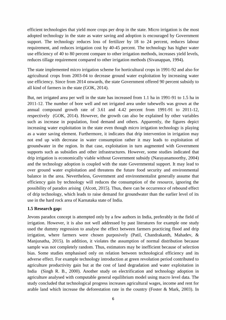
also the worldwide. Figure 1 represents the allocation of irrigation water out of total water
used in selected countries. Figures depicts that, more than 80 percent of total water used to
for irrigation in developing countries such as India, China and Egypt against the developed
countries such as Netherlands, France, and UK were using less than 30 percent. It concludes
that developing and agrarian economies uses more water for irrigation compare to other ones.
At present, India is the highest water user for irrigation in the world. India was one of the
agrarian economies at green revolution period. The agriculture and allied sectors share was
42.56 to 27.13 percent to the country’s total GDP for the period 1960 to 1996 respectively
(Planning Comission, 2017). By the end of 2000, availability of annual renewable water per
person was less than 500 m3, which was less than many parts of the world, namely United
States, Europe, Central Asia, and some parts of Africa (Carmen, 2000).
Groundwater occupied the large share among the various sources of irrigation in India, in
2000 groundwater accounted 35 percent share to the total irrigated area. Number of
groundwater abstraction structures has increased in India from 1 million in 1950 to 17 million
11
in 1997. In addition, irrigation potential with groundwater has increased from 6 million
hectares (M ha) to 36 M ha for the same period (Igor & Lorne, 2004).
Figure 1: Percent share of irrigation to the total water used in selected countries, 1995
Source: Saeijs & Van, 1995
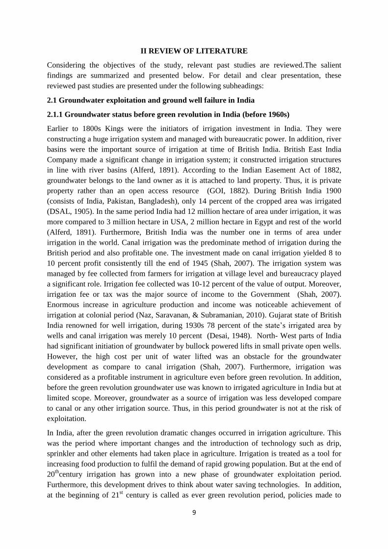
Figure 2 indicates trend in growth of net irrigated area between period 1960-61 and 2011-12
in India. At the beginning of green revolution 1960-61, canals were the major source of
irrigation while area under bore well irrigation was negligible.
Figure 2: Net irrigated area (000’ hectares) over the years in India
Source: Ministry and Farmers Welfare.
0
10
20
30
40
50
60
70
80
90
100
India China Egypt Netherlands France UK
Per
cen
t o
f to
tal
use
0
10000
20000
30000
40000
50000
60000
70000
80000
1960-6
1
1962-6
3
1964-6
5
1966-6
7
1968-6
9
1970-7
1
1972-7
3
1974-7
5
1976-7
7
1978-7
9
1980-8
1
1982-8
3
1984-8
5
1986-8
7
1988-8
9
1990-9
1
1992-9
3
1994-9
5
1996-9
7
1998-9
9
2000-0
1
2002-0
3
2004-0
5
2006-0
7
2008-0
9
2010-1
1
2012-1
3
Net
irr
igate
d a
rea (
'000 h
a)
Net irrigated area by tubewells ( in ' 000 Hectares)
Net irrigated area by canals ( in ' 000 Hectares)
Total Net Irrigated Area (in ' 000 Hectares)
12
Since after1966-67, groundwater source was taking an exponential growth, while the area
under canal source was not decreasing but the growth was less than the groundwater source.
In addition, decreasing trend in area under canal irrigation was noticeable after 2000-01.
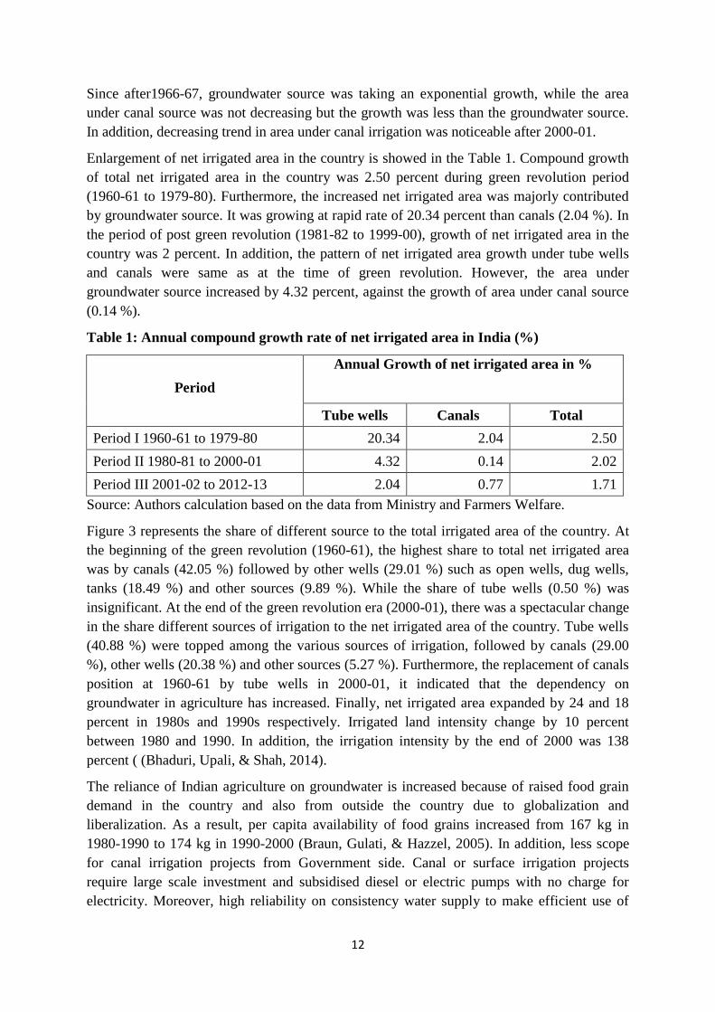
Enlargement of net irrigated area in the country is showed in the Table 1. Compound growth
of total net irrigated area in the country was 2.50 percent during green revolution period
(1960-61 to 1979-80). Furthermore, the increased net irrigated area was majorly contributed
by groundwater source. It was growing at rapid rate of 20.34 percent than canals (2.04 %). In
the period of post green revolution (1981-82 to 1999-00), growth of net irrigated area in the
country was 2 percent. In addition, the pattern of net irrigated area growth under tube wells
and canals were same as at the time of green revolution. However, the area under
groundwater source increased by 4.32 percent, against the growth of area under canal source
(0.14 %).
Table 1: Annual compound growth rate of net irrigated area in India (%)
Period
Annual Growth of net irrigated area in %
Tube wells Canals Total
Period I 1960-61 to 1979-80 20.34 2.04 2.50
Period II 1980-81 to 2000-01 4.32 0.14 2.02
Period III 2001-02 to 2012-13 2.04 0.77 1.71
Source: Authors calculation based on the data from Ministry and Farmers Welfare.
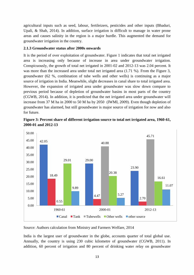
Figure 3 represents the share of different source to the total irrigated area of the country. At
the beginning of the green revolution (1960-61), the highest share to total net irrigated area
was by canals (42.05 %) followed by other wells (29.01 %) such as open wells, dug wells,
tanks (18.49 %) and other sources (9.89 %). While the share of tube wells (0.50 %) was
insignificant. At the end of the green revolution era (2000-01), there was a spectacular change
in the share different sources of irrigation to the net irrigated area of the country. Tube wells
(40.88 %) were topped among the various sources of irrigation, followed by canals (29.00
%), other wells (20.38 %) and other sources (5.27 %). Furthermore, the replacement of canals
position at 1960-61 by tube wells in 2000-01, it indicated that the dependency on
groundwater in agriculture has increased. Finally, net irrigated area expanded by 24 and 18
percent in 1980s and 1990s respectively. Irrigated land intensity change by 10 percent
between 1980 and 1990. In addition, the irrigation intensity by the end of 2000 was 138
percent ( (Bhaduri, Upali, & Shah, 2014).
The reliance of Indian agriculture on groundwater is increased because of raised food grain
demand in the country and also from outside the country due to globalization and
liberalization. As a result, per capita availability of food grains increased from 167 kg in
1980-1990 to 174 kg in 1990-2000 (Braun, Gulati, & Hazzel, 2005). In addition, less scope
for canal irrigation projects from Government side. Canal or surface irrigation projects
require large scale investment and subsidised diesel or electric pumps with no charge for
electricity. Moreover, high reliability on consistency water supply to make efficient use of
13
agricultural inputs such as seed, labour, fertileizers, pesticides and other inputs (Bhaduri,
Upali, & Shah, 2014). In addition, surface irrigation is difficult to manage in water prone
areas and causes salinity in the region is a major hurdle. This augmented the demand for
groundwater irrigation in the country.
2.1.3 Groundwater status after 2000s onwards
It is the period of over exploitation of groundwater. Figure 1 indicates that total net irrigated
area is increasing only because of increase in area under groundwater irrigation.
Conspicuously, the growth of total net irrigated in 2001-02 and 2012-13 was 2.04 percent. It
was more than the increased area under total net irrigated area (1.71 %). From the Figure 3,
groundwater (62 %, combination of tube wells and other wells) is continuing as a major
source of irrigation in India. Meanwhile, slight decreases in canal share to total irrigated area.
However, the expansion of irrigated area under groundwater was slow down compare to
previous period because of depletion of groundwater basins in most parts of the country
(CGWB, 2014). In addition, it is predicted that the net irrigated area under groundwater will
increase from 37 M ha in 2000 to 50 M ha by 2050 (IWMI, 2009). Even though depletion of
groundwater has alarmed, but still groundwater is major source of irrigation for now and also
for future.
Figure 3: Percent share of different irrigation source to total net irrigated area, 1960-61,
2000-01 and 2012-13
Source: Authors calculation from Ministry and Farmers Welfare, 2014
India is the largest user of groundwater in the globe, accounts quarter of total global use.
Annually, the country is using 230 cubic kilometre of groundwater (CGWB, 2011). In
addition, 60 percent of irrigation and 80 percent of drinking water relay on groundwater
42.05
29.00
23.90
18.49
4.47 2.70
0.55
40.88
45.71
29.01
20.38
16.61
9.89
5.27
11.07
0.00
5.00
10.00
15.00
20.00
25.00
30.00
35.00
40.00
45.00
50.00
1960-61 2000-01 2012-13
Canal Tank Tubewells Other wells other source

14
(World Bank , 2012). Number of bore wells increased from 0.1 million in 1960 to 25 million
in 2010 (Chandrakanth, 2015). As a result of continuous increase in groundwater extraction
and the use is not only for the irrigation but also for other purposes such as industries,
drinking etc. This ended up in depletion of groundwater resource all over the country.
According to national assessment of 2004, 29 percent of groundwater blocks were reported as
semi-critical, critical and over-exploited in the country. If the present trend of groundwater
use continues which leads to critical condition of 60 percent aquifers in the country (World
Bank , 2012).
2.1.4 Extent of groundwater over-exploitation and its consequences in India
Continuous increasing in scope for groundwater not only led to increase in area under
irrigation but also had consequences on groundwater resource degradation (Chandrakanth,
2015). Groundwater is an important natural resource of every nation. Preferably, for the
tropical countries namely India as agriculture is gambling with the monsoons in the country.
Furthermore, the country has to feed the 1.3 billion people. Moreover, this dependency ended
up in exploitation of groundwater resource in the country. India is exploiting annually 245
BCM, which is more than China’s (135 BCM) annual withdrawal of groundwater (SANDRP,
2016). Aquifer is a rock situated under the ground, which transmits the water to wells. The
countries groundwater system is divided into two, namely hard-rock aquifers of peninsular
India and alluvial aquifers of Indo-Gangetic plains. Hard-rock areas aquifers shares 65
percent of the country’s surface area, major parts of this situated in peninsular India
(Chandrakanth, 2015). The range of exploitation varies across the country because of
different aquifer system (Suhag, 2016). Places falls under the Gangetic- Alluvial plains for
example Bihar was entirely safe compare to western Indus alluvial regions such as Punjab
where 75 percent of regions were over exploited. In addition, states of hard rock areas such as
Gujarat, Haryana, Karnataka, Tamil Nadu, Rajasthan and Andhra Pradesh also showed sign
of over exploitation (Sundarajan, Patle, Trishikhi, & Purohit, 2017). Finally, 15 states out of
30 states and 2 out of 8 Union territories of India are classified under over- exploited category
(SANDRP, 2016).
Table 2 represents the severity of groundwater exploitation for the different periods from
1995 to 2011. At 1995, less than 10 percent of districts need the recommendations for future
groundwater use. In addition, only 3 percent of country’s districts were over exploited. But
the figures after 2000 onwards depicts that groundwater exploitation widens in the country.
Furthermore, more than 25 percent of the country’s area has to take measures for
groundwater conservation. By the end of 2011, 15 percent of India’s area has marked under
over-groundwater exploitation. Among Indian states, the over-exploitation of groundwater
topped in Northern-Western plain (72.56 %) followed by Western arid region (37.23 %) and
Southern peninsular India (22.2 %) (CGWB, 2014) In addition, at the over exploited regions,
there was a significant fall in aquifers property before and after monsoons arrival. Moreover,
over the year groundwater development was raising at 4 times in all over the country
(Sundarajan, Patle, Trishikhi, & Purohit, 2017). In addition, the declined water yield of the
bore wells, it has been recorded in 56 percent of bore wells from 2003 to 2013. Preferably, in
the case of hard rock areas such as Tamil Nadu (76 %), Kerala (71 %), Karnataka (69 %) and

15
Haryana (65 %) bore well yield declined significantly (CGWB, 2014). Between period 2002
and 2012, it has been noted that farmers were pumping out groundwater 8 percent. It was
more than average annual rate of groundwater replenished; this caused a drop of water table
at the rate more than 1.5 meters per year (Postel, 2015).
Table 2: Comparative status of groundwater over-exploitation in India from 1995 to
2011
Level of
Groundwater
Development
Explanation
% of
districts in
1995
% of
district in
2004
% of
district in
2009
% of
district in
2011
0 – 70 %
Areas which have ground
water potential for
development
92.00 73.00 72.00 71.00
70 – 90 %
Areas where cautious ground
water development is
recommended
4.00 9.00 10.00 10.00
90 – 100 %
Areas which need intensive
monitoring and evaluation
for ground water
development
1.00 4.00 4.00 4.00
>100 %
Areas where future ground
water development is linked
with water conservation
measures
3.00 14.00 14.00 15.00
Source: CGWB, 2014.
Depletion of natural resource disturbs the ecosystem balances and leads to negative
consequences on environment. Groundwater is an important and fundamental environmental
resource and extensive demanded one from mankind. Continuous increasing in extraction of
groundwater has negative effects such as drinking water problem, increasing the water
extraction cost, frequent well failure, reducing command area of well, increasing inequity for
assessing well water and in addition ecological degradation such as soil salinity, decreasing
groundwater table (Kumar M. D., 2007; Kumar, Singh, & Sharma, 2005). In addition,
insufficient availability of water per head per year, for example amount of annual per capita
availability was decreased from 6042 cubic meter in 1947 to 1545 cubic meter in 2011
(Vishwa, 2014). Degradation of groundwater quality is another important outcome of
groundwater depletion. For example, 82 percent of area in Karnataka and Tamil Nadu is
under high groundwater development. The areas are suffering from salinity and water quality
problems (Sundarajan, Patle, Trishikhi, & Purohit, 2017).
South West and Central India has water tables at lower or deeper level. Especially, in the case
of Southern region 30 percent of groundwater table is situated at the depth of more than 60
meters (Singh P. , 2015). Depletion of the water table makes farmers to drill deepened bore
16
well. In addition, deepened drillings increases the cost of drilling and cost of irrigation
(Viswanathan, Kumar, & Narayanamoorthy, 2016). In addition, the over-exploitation adds
more to the groundwater extraction cost, because well has to drill deep and it requires more
fixed cost for drilling and adds more to maintenance cost for pumping water (Nagaraj &
Chandrakanth, 1997). The growth of shallow and deep tube wells in 1980s was 7.2 and 5.3
percent respectively while growth of dug wells was 1.8 percent (Nagaraj, Chandrakanth, &
Gurumurthy, 1994). A study indicated that over the years bore wells of 10 meter and more
depth has increased compared to the ones of less than 10 meter depth. Preferably, tubewells
with more than 60 meter increasing at rapid rate compares to the bore wells of depth between
10 to 60 meters. Meanwhile, the decreased share of bore well depth less than 10 meter
(Singh P. , 2015). The water which is extracted from deeper depths usually evidence the
contamination with high fluoride level, arsenic content and other harmful chemicals
(Wyrwoll, 2012). Poor quality of bore well water not only affecting crop yield but also causes
diseases to human (Reddy & Gunasekar, 2013). All kind of water bodies are related to each
other, thus groundwater overuse which is ending up in drying of surface water bodies such as
lakes, rivers, ponds and other water bodies (GWF, 2017).
2.2 Probability of well failure in India
Poor aquifer property coupled with exploitation of groundwater will augmented the problem
of well drying and failure in the country. Groundwater depletion and poor water table
development cause the wells to dry up and failure of bore wells at initial and pre-mature
stages. Well failure is serious outcome of groundwater overuse and hurdle to the farmers’
income in India. Especially, in hard rock areas of the country such as Karnataka, Tamil Nadu,
and Andhra Pradesh etc. Probability of getting a successful bore well is very low in the case
of peninsular hard-rock areas (Nagaraj, Marshal, & Sampath, 1999). At the beginning of
green revolution, bore wells drilled were not lost after 20 years age, but since after 2000 bore
well’s life is becoming shorter less than 8 years and even failures at drilling (Nagaraj,
Chandrakanth, & Gurumurthy, 1994). The failures is adding cost to the farmers cost of
production and reduces their net income. The cost of production or irrigation cost increase
with increase in number of well failures. A study indicated that the average rate of well
failure in Tamil Nadu state of India was 47 percent for open wells and 9 percent for tube
wells. In addition, the total cost of depletion of new wells varies from Rs. 1999 to Rs. 90975,
respectively (Palanisami, Vidhyavathi, & Ranganathan, 2008). Depletion of groundwater
table lead a way for resource rich farmers to invest more on deepening and drilling additional
bore well and is coupled with installation of high powered submersible pump to lift water
from more depth. Furthermore, this raises the question of equality and equity with respect to
resource poor farmers for accessing groundwater (Nagaraj & Chandrakanth, 1997). Excessive
and continuous pumping in a bore well is causing to dry up neighboring bore well, where
bore wells shared common aquifer because of well interference. In addition, less isolation
distance between wells is leading to initial and pre-mature failure of bore wells in hard rock
areas of India. For example, in Karnataka probability of well failure was estimated with
negative binomial distribution. The probability of well failure was 40 percent, that means for
every 100 wells drilled there was 40 percent possibility of well failure (Chandrakanth, 2015).
Another study indicated that growth of number of wells is not ended up in increasing area
17
under irrigation due to rise in number of well failure. In addition, less discharge from bore
well, failure in successful installation of bore well, seasonal failure of open wells augmented
the extra burden on farmers (Bassi, Vijayshankar, & Kumar, 2008). Furthermore, small
farmers are the worst sufferer’s due to well failure (Anantha & Raju, 2008). However, the
extent of failure varies with level of ground water development in the region (Nagaraj,
Chandrakanth, & Gurumurthy, 1994).
Therefore, well failure is one of main outcome of groundwater overuse. This study is making
a modest attempt to find the bore well failure and its probability in the study area. According
to the past studies negative binomial distribution methodology is captured to find out extent
of tube wells failure in the study area.
2.3 Emergence of water saving technologies in India
2.3.1 Importance of water saving technologies in India
If the above trend of groundwater extraction continues, it will leave the future generation
without sufficient water. By end of 2025, annual per capita availability of water decrease to
1399 cubic meters against the availability of 1588 cubic meter in 2011 (WRI, 2016). India is
the second largest country in terms of population and food security is an important addressing
issue in the country. In addition, an estimate indicates that India population will be 1.6 billion
at the end of 2050 (Sinead, 2014; Balyan, 2016). As population grows, the demand for
groundwater also increases. It has been estimated that 30 percent will be decline in
groundwater availability per person in the country by 2050 (Upali, Shah, Hugh, & Anand,
2007). In addition, an estimate shows that share of groundwater in to the total irrigated area
will decreases from 60 percent in 2012 to 51 percent 2025. Therefore, efficiency of
groundwater irrigation should be increase to 75 percent by 2025 from water use efficiency of
60 percent in 2006 (Upali, Shah, Hugh, & Anand, 2007). As a result, it will threaten the
country’s future food security. Thus, it is important to increase water use efficiency rather
than increasing area under irrigation without compromising crop productivity. The
government intended to develop and promote of high water use efficient technologies and
irrigation methods.
2.3.2 Water saving technologies adopted in India
Water efficient technologies are looking from the side of water saving in India. ‘More crops
per drop’ will solve the food security problem on one way and conserve water/groundwater
resource on another way. Hence, it necessitates the adoption of new innovative products to
reduce water usage. Flood irrigation is the conventional irrigation practice in the country’s
agriculture, where water efficiency is less than other methods. Among conventional methods
of irrigation water use efficiency was 35 to 40 percent (Narayanmoorthy, Indian Water
Policy at the Crossroads: Resources, Technology and Reforms, 2016). In India, different
kinds of water saving technologies are recognized. Namely, moisture storage pits: increase
groundwater table, raises irrigation activity and increases farm productivity. Rain water
harvesting: increases groundwater table and decreases run-off in the farm. Zero tillage
practice: is also aiming at conserving soil, water and ecosystem with little interference of
tillage practices. It has been proved that 25 percent saving of irrigation water from zero
18
tillage and grain yield increases more than 50 percent (KINSPARC, 2009). On-farm rain
water management: is excavating small ponds to collect rain water. This will help in
recharging groundwater table and also useful for raising second crop after rainy season.
Watershed management is also to conserve and to recharge groundwater. However, all these
were not appreciated by farmers even though encouragement from government side. The
governmental programmes such as in 1992 initiated rainwater harvesting programme to
recharge groundwater, watershed programmes to conserve soil and water and many other.
But, these are failing to achieve 100 percent of their targets because of poor response from
end users (farmers).
2.3.3 Emergence of micro-irrigation technology in India
Micro-irrigation is seen as a boom for water saving by increasing water use efficiency.
Sprinkler and drip are the main elements of micro irrigation that have been operating in
Indian irrigation sector. In addition, to having high water use efficiency, the technologies
increase crop yield at reduced cost of cultivation compare to conventional irrigation methods
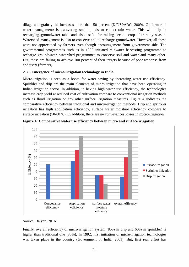
such as flood irrigation or any other surface irrigation measures. Figure 4 indicates the
comparative efficiency between traditional and micro-irrigation methods. Drip and sprinkler
irrigation has high application efficiency, surface water moisture efficiency compare to
surface irrigation (50-60 %). In addition, there are no conveyances losses in micro-irrigation.
Figure 4: Comparative water use efficiency between micro and surface irrigation
Source: Balyan, 2016.
Finally, overall efficiency of micro irrigation system (85% in drip and 60% in sprinkler) is
higher than traditional one (35%). In 1992, first initiation of micro-irrigation technologies
was taken place in the country (Government of India, 2001). But, first real effort has
0
10
20
30
40
50
60
70
80
90
100
Conveyance
efficiency
Application
efficiency
surfece water
moisture
effciency
overall efficency
Eff
icie
ncy
(%
)
Surface irrigation
Sprinkler irrigation
Drip irrigation

19
established in 2006 through government launched centrally sponsored programme for micro-
irrigation. It was upgraded in 2013-14 as National Mission on Micro Irrigation (NMMI)
(Goverment of India, 2015). In 2015, it was merged with National Mission for Sustainable
Agriculture (NMSA). Pradhan Mantri KrushiSinchayee Yojana (PMKSY) was launched in
2015 and is an ongoing project in the country. The programme aimed to create infrastructure
to adopt micro-irrigation technology and subsidy being the main element of the programme.
Furthermore, Government of India has been making continuous effort to encourage farmers
to adopt micro irrigation technology to save groundwater or to reduce groundwater use
(Goverment of India, 2015).
Noticeable growth of area under micro-irrigation has taken place in India (Narayanamoorthy,
2004).in addition, appreciable growth of area under micro-irrigation is noticeable since after
2005. The area was increased from 3.09 million hectare in 2005 to 7.73 million hectare 2015
at the rate of 9.6 percent. However, the country’s penetration in micro irrigation technologies
was 5.5 percent less than the rest of the world such as Israel, USA, Russia, Spain and China
(Balyan, 2016). In 2015, the share of drip and sprinkler to the country’s total micro irrigation
area was 43.6 and 56.4 percent respectively. But, growth of drip irrigation was 9.85 percent
against 6.6 percent in sprinkler irrigation for the period 2012-2015. The area under drip
irrigation showed a tremendous growth. It is evident by increased area under micro irrigation
from 40 ha in 1960 to 3.37 million hectare in 2015. Indian states such as Maharashtra (94000
ha), Karnataka (66000 ha) and Tamil Nadu (55000 ha) have larger area under drip irrigation
than rest of the country (ICAR, 2015). Moreover, drip irrigation method (85 %) has high
water use efficiency compares to sprinkler irrigation (60 %). In addition, sprinkler method
has limited scope under windy weather and undulating topography. Furthermore, drip
irrigation (9.85 %) is growing faster than sprinkler irrigation (6.6 %) from field crops to
perennial plantations. In the country, Karnataka state is situated in the southern peninsular
region with more area under drip than sprinkler. It makes more sense to analyse the research
objects under drip irrigation technology than sprinkler one. Thus, the main focus of study is
testing the Jevons paradox in drip irrigation rather sprinkler irrigation.
2.3.4 Factors determining drip irrigation adoption in India
Installations of micro-irrigation depend on various factors and vary with different climatic
conditions (Dhawan, 2000). A study indicated that family size and demographic structure,
human capital, ownership on agro wells, depth of well, cropping pattern, other socio-
economic variables such as caste, poverty index, off-farm and non-farm economic variables
are important to determine the adoption of micro-irrigation (Regassa, Upadhyay, & Nagar,
2005). The results of a logit function indicate that the deeper the well, the higher will be the
probability to adopt, and also the higher the share of fruits, vegetables and commercial crops
the higher the probability of drip adoption and also socio-economic variables had significant
effect on technology adoption (Regassa, Upadhyay, & Nagar, 2005). In another case, it
depends on type of crop grown and better suited for horticulture crops than field crops. In
addition, range of physical, socio-economical and financial variable decides the crop and its
area under irrigation through micro-irrigation (Dhawan, 2000). Age of the farmers, farm size,
wider crops, and non-farm income has positive effect on drip technology adoption in India.

20
The size of farm indicates wealth of a farmer. However, small and marginal farmers
enthusiastic to adopt drip technology but they need support for initial investment (Goyal,
2015). Government subsidy is also one of the important factors for having micro-irrigation
technology. The results showed that years of extra subsidy offered from the government
showed higher percentage of drip and sprinkler adoption compare to the year without subsidy
(Viswanathan, Kumar, & Narayanamoorthy, 2016; Kumar, Hugh, Sharma, Upali, & Singh,
2008). However, some studies disproved effect of subsidy in drip implementation
(Narayanamoorthy, 2004 & 2008; Sivanappan, 1994). In another study indicated the other
factors with above factor of drip adoption such as power of pump owned and years of
schooling of household head, dependency ratio influences the adoption. Furthermore, caste,
poverty index and share of area under vegetables, power of pump owned had positive and
significant effect on probability of adoption while area under cereals had negative and
significant effect on adoption (Namara, Nagar, & Upadhyay, 2007).
2.3.5 Drip irrigation method as a water saving technology
Micro-irrigation is a method where water is supplied directly to the root system in the form of
droplets. The previous section dealt with the advantages of micro-irrigation over flood
method. Preferably, drip irrigation results in very high water use efficiency of about 90 to 95
percent (ICAR, 2015). Furthermore, it saves water by 40 to 80 percent and yield will
increase up to 100 percent in different crops (Narayanamoorthy, 2004). Drip irrigation is
proved as a technically feasible and socially acceptable type of micro irrigation not only for
large farmers but also for the small farmers in India (Sivanappan, 1994). In addition, more
benefits of micro-irrigation realised in semi-arid and arid region especially in wide spaced
crops (Kumar, Hugh, Sharma, Upali, & Singh, 2008). It saves energy requirement (30.5 %),
reduces fertilizer consumption (28.5 %), productivity increases in fruits (42.4 %) and
vegetable crops (52.7 %), and reduces irrigation cost (31.9 %) (Balyan, 2016). For example,
cost of cultivation of drip adopted farmers in coconut and banana crop was 9.1 and 56.4
percent respectively less than the non-adopters (Goyal, 2015). In another situation, micro-
irrigation in tomato saved 21 percent of water and increased yield by 27 percent (Dalvia,
Tiwarib, Pawadea, & Phirkea, 1999). Water saving in micro-irrigation varies across the crops
from 12 to 79 percent and increase in yield varies from 12 to 179 percent (Narayanamoorthy,
2004). It has been proved that incremental benefit-cost ratio for different crops varies from
1.35 to 13.35 excluding water saving and with water saving ratio is 2.78 to 32.32
(Sivanappan, 1994). An estimate indicated that water saving by drip irrigation was noted as
11.271 million hectare meter and which can potentially irrigate area of 11.22 million hectare
under flood method of irrigation or 24.12 million hectare by drip method (Narayanamoorthy,
2004). Since, the study emphasis on further enlargement of irrigated area by saved water, it
deviates the technology as profit rising element rather than water saving one. A study
indicated that 3 percent increase in the ground water use over the total mean annual
extraction after the technology adoption. In other parts of the world, micro-irrigation
technology adoption leads to increase in the average area under irrigation (Pfeiffer &
Cynthia, 2013). This contradict findings are placed the drip irrigation under debate of water
saving technology or water exploiting element?
21
2.4 Jevons Paradox in technology innovation and its relevance to drip irrigation
The reviewed literature indicates the positive and potential effect of drip technology.
However, the studies are looking technology from one face as water saving technology rather
than the income earning one. Drip irrigation method is not only a saving technology
meanwhile it is increasing the farmers’ income by decreasing cost of cultivation of crops and
increasing the crop productivity. The increased efficiency lead to decrease in irrigation cost,
in the other words it decreases the price of groundwater. As price of groundwater goes down,
it increases the quantity demanded. Efficiency can lead to more use of groundwater to
produce larger quantity of crop than initial production level this is termed as rebound effect
of drip technology. In addition, Governmental support to promote water efficient
technologies can couple the problem of groundwater exploitation rather than conservation.
Furthermore, technology is not always lead to reduce consumption of resource units. This is
the situation of Jevons paradox. There is a chance of occurrence of the paradox in the study
area.
Occurrence of Jevons paradox is not new to agriculture field. Agricultural land intensification
and increased productivity may lead to increase in land use to produce more units in order to
earn higher profit (Lambin & Meyfroidt, 2011). Agriculture intensification is necessary to
promote food security on one way meanwhile decreases pressure on land. But, this is may
also lead to increases pressure on forest land without complementary policies (Ceddiaa,
Sedlaceka, Bardsleyb, & Gomez-y-Palomac, 2013). It is again proved that land
intensification will not lead to decline pressure on land use at national level over the year
(Rudela, et al., 2009). A study indicated that conservation, simplification, pricing and
innovations can only serve for shorter term. However, in long term these can result contradict
results (Tainter, 2011). Modernisation of economy is employing the energy efficient
technologies to reduce resource use but it has been proved that there is linear relationship
between resource use and economic growth and agriculture production for all years for Costa
Rica, Korea, Mexico, the Netherlands and the United States (Young, Charles, Hall, & Lopez,
1998). Similar results were recorded in the case of West Europe, Middle East, South Africa,
and in some Asian countries. In addition, a study showed the positive association between
energy consumption and economic growth over the years with energy efficient technologies
(Polimeni, Raluca, & Polimeni, 2006).
Some literature proved that the existence of Jevons paradox in irrigation technologies or
irrigation modernization. A study indicated that actually objective of irrigation modernization
is to increase efficiency without compromising farm income. But, contradict results recorded
in the case of irrigation technologies (Gomez & Dinisio, 2015). In another case, dropped
nozzles implemented to increase irrigation efficiency and to save groundwater in Western
Kansas. The results indicated that groundwater consumption did not decreased rather it
increased the use due to change in cropping pattern (Pfeiffer & Cynthia, 2013). Similar
results also found in Europe after irrigation technologies promoted by European Commission.
In addition, it also indicated that drip and sprinkler irrigation will reduce water consumption
only if restriction imposed on new irrigated area (Berbel & Mateos, 2014). In the case
Northern Basin of Australia, a study concluded that greater the technology change in
22
irrigation higher will be the consumptive demand for land and water because farmers switch
to perennial crops with government incentives (Loch & Adamson, 2015). However, some
studies disproved the existence of the paradox. For instance, in the case of irrigation
modernization in Spain depicted that the country saved 12 percent water from modernization
of irrigation methods ( (Dumont, Mayer, & Lopez, 2013). Similar results are recorded with
dummy regression for farmers practicing flood and drip irrigation. The results represent that
thearea under drip irrigation was not increased thus there is no existence of rebound or Jevons
paradox in drip irrigation technology in India (Patil, Chandrakanth, Mahadev, & Manjunatha,
2015).
The above literature indicates that very few studies carried out on drip irrigation and the
Jevons paradox. There are limitations; some studies attempted using macro level data but
limited scope at farm level studies. The present study is an attempt to test rebound or Jevons
paradox in drip irrigation technology of hard rock areas of India by using micro level data.
The study main focus is to analyse whether water consumption is increased in the case of drip
irrigation farmer or not by comparing with control group or farmers following conventional
irrigation method.

23
III METHODOLOGY
In this chapter, a brief description of study area, sampling method and tools employed
for data analysis are presented under the following heads.
3.1 Description of the study area
3.2 Sampling Procedure
3.3 Analytical techniques
3.1 Description of the study area
The study is based hard rock areas of Karnataka state of India. Karnataka state is one among
30 states of India. It has 30 districts, 270 towns and 29406 villages (GOI, 2015). Bangalore is
the capital city of the state. The city is one of the largest metropolitan cities in India (GOI,
2015). In India, the state stands at 8th
position in terms of population (Census of India, 2011).
Kannada is the most spoken language in the state. The state is one among the rapid growing
states of India with the GSDP growth of 8.2 percent in 2010-11, which was more than the
country’s growth rate (GOI, 2015). Out of total GSDP, 16 percent was contributed by
agriculture and its related sectors.
The state is chosen for the study, because groundwater status is at the critical limit. Rainfall
occurrence is erratic in the state. Rainfall varies across the state from 569 mm in East to
4029 mm in west parts of the state. The annual rainfall in the state is 1138 mm (Water
Resources Department, 2002; Chandrakanth, 2009). This lead to more dependency on
groundwater in the state compare to rest of the country. The most parts of Karnataka4,
groundwater quality declined to critical level (CGWB, 2014). In addition, it created the
serious water problems ranges from 50-79 percent. Out of which, fluoride, arsenic and other
contaminations are noticeable (Parisaramahiti, 2017). Nonetheless, water resource is very
important for the state, preferably groundwater as it is playing an important role in the state
agriculture production. Furthermore, the state is one of the fast-growing economies in the
country (IBEF, 2010). The agriculture snapshot of the state is presented as below.
3.1.1 Agriculture profile of Karnataka state in India
The state is blessed with tropical climate and has into three seasons, rainy or monsoon (June
to October), winter (November to January) and dry or summer (February to May).
Agriculture is the lifeblood of rural people in the region. According to the 2011 census, the
state agriculture supports 13.74 million workers, out of which 26.61 percent were cultivars
and 25.67 percent were agricultural workers. Furthermore, it provides employment to more
than 50 percent of the state population (Census Population, 2011). The south-west monsoons
are playing a vital role in cultivation of crops. In addition, the state is placed at 7th
position in
terms of geographical area in India. Area under agriculture cultivation accounts to 64.5
percent to the total geographical area (GOI, 2015). In addition, out of total land under
cultivation 26.5 percent was the area under irrigation (Bhende, 2013).
4 Bagalkot, Bengaluru urban, Vijayapur, Chamarajnagar, Chitradurga, Haveri, Mandya, Davangere, Kodagu,
Kolar, Raichur, and Koppal Districts.
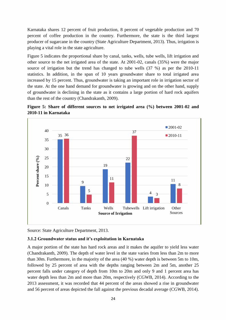
24
Karnataka shares 12 percent of fruit production, 8 percent of vegetable production and 70
percent of coffee production in the country. Furthermore, the state is the third largest
producer of sugarcane in the country (State Agriculture Department, 2013). Thus, irrigation is
playing a vital role in the state agriculture.
Figure 5 indicates the proportional share by canal, tanks, wells, tube wells, lift irrigation and
other source to the net irrigated area of the state. At 2001-02, canals (35%) were the major
source of irrigation but the trend has changed to tube wells (37 %) as per the 2010-11
statistics. In addition, in the span of 10 years groundwater share to total irrigated area
increased by 15 percent. Thus, groundwater is taking an important role in irrigation sector of
the state. At the one hand demand for groundwater is growing and on the other hand, supply
of groundwater is declining in the state as it contains a large portion of hard rock aquifers
than the rest of the country (Chandrakanth, 2009).
Figure 5: Share of different sources to net irrigated area (%) between 2001-02 and
2010-11 in Karnataka
Source: State Agriculture Department, 2013.
3.1.2 Groundwater status and it’s exploitation in Karnataka
A major portion of the state has hard rock areas and it makes the aquifer to yield less water
(Chandrakanth, 2009). The depth of water level in the state varies from less than 2m to more
than 30m. Furthermore, in the majority of the area (40 %) water depth is between 5m to 10m,
followed by 25 percent of area with the depths ranging between 2m and 5m, another 25
percent falls under category of depth from 10m to 20m and only 9 and 1 percent area has
water depth less than 2m and more than 20m, respectively (CGWB, 2014). According to the
2013 assessment, it was recorded that 44 percent of the areas showed a rise in groundwater
and 56 percent of areas depicted the fall against the previous decadal average (CGWB, 2014).
35
9
19
22
4
11
36
5
11
37
3
8
0
5
10
15
20
25
30
35
40
Canals Tanks Wells Tubewells Lift irrigation Other
Sources
Per
cen
t sh
are
(%
)
Source of Irrigation
2001-02
2010-11
25
According to the dynamic report on groundwater of Karnataka 2014, represents that 80
percent of the areas were over exploited (CGWB, 2014). In the state 10 areas categorized as
critical, 17 as semi-critical and 127 named as safe with respect to groundwater use (Girish,
2009). Furthermore, in 2014 out of 174 taluks of the state 90 were reported as groundwater
overused areas (Shivaraj, 2014).
Karnataka state is one of the largest state having area under micro-irrigation (0.94 m ha) in
India (GGGI, 2015). The state is the fourth largest state in area under drip irrigation (0.39 m
ha) next to Maharashtra (0.88 m ha), Andhra Pradesh (0.84 m ha) and Gujarat (0.42 m ha)
(GGGI, 2015). The state Government is promoting micro-irrigation with an objective to
reduce the groundwater consumption for irrigation. The Government attempted micro-
irrigation development at various levels. Agriculture and horticulture are two main key
sectors in promoting micro-irrigation, preferably drip method through subsidized
programmes (GOI, 2015).
In order to fulfil the research objective, Chikkaballapura district of Karnataka state has
chosen as sample district. Figure 6 depicts the study area.
3.1.3 Agriculture profile of Chikkaballapura district of Karnataka, India:
Chikkaballapura district of Karnataka state is placed in southern part. It is newly formed
district since 2007 and previously it was under Kolar district. The district has 6 taluks
namely, Chikkaballapura, Gauribidanur, Shidlaghatta, Chintamani, Gundibanda and
Bagepalli. According to the 2011 census, the district has 1513 villages (Directorate of Census
Operations, 2011). In addition, population of the district was 1.25 million and 298 persons
were living per square meter (Kallapur, 2012). The district achieved gross domestic product
of INR 3.5 billion in 2012-13 and same year annual per capita income in the district was INR
44183 (UASB, 2014). Furthermore, the area is just 50 km away from metropolitan city
Bangalore. It is also well connected with highways (Bangalore-Hyderabad) and railways.
Thus, there is a huge scope for horticulture crops such as vegetables, flower, fruits and other
crops. Livestock has emerged as an important subsidiary occupation of farmers and other
members in the district.
The total geographical area of the district is 0.40 m ha; area under crop cultivation shares the
highest (52 %), followed by other uncultivated land (33 %) and forest land (12 %). Red-
loamy, red-sandy and mixed red are the major soil types in the region. The normal annual
rainfall was 677 mm but actual received was 424 mm in 2012-13. Net cultivated area was
0.19 m ha, out of which 27 percent was under irrigation (GOK, 2016). The major crops in the
area are ragi, maize, oilseeds, fruits, vegetables, fruits and commercial crops. Figure 7
represents the cropping pattern of the study area. In crop year 2012-13, crop cultivation was
dominated with cereals (60 %) followed by oilseeds (13 %), pulses (7 %) and least by
commercial crops5 (0.09 %) (UASB, 2014).
5 Seasonal flower crops such as Marigold, Gladiolus and commercial crops such as cotton, sugarcane and other
crops

26
Figure 6: Map showing study area in Karnataka state of India
Source: Author

27
Figure 7: Cropping pattern of Chikkaballapura district 2012-13, Karnataka.
Source: UASB, 2014; GOI, 2015.
3.1.4 Groundwater use in Chikkaballapura district of Karnataka
Groundwater is playing a vital role in irrigated agriculture of the district. Net groundwater
availability in the region was 28426 ha m, existing groundwater available for all uses was
40060 ha m and the available resources for future was 1699 ha m. Groundwater levels varies
from 1.8m to 11.35m in pre-monsoon against deviations of 0.87m to 13.35m in post-
monsoon seasons (Ministry of Water Resources, 2012). Decadal mean water depth fluctuates
from 0-2 m and 2-4 m during pre-monsoon and post-monsoons, respectively. Bore wells are
the sole source of irrigation; they accounts for 99 percent of net irrigated area in the region.
There were 29985 irrigation tube wells, the ratio of gross irrigated area to bore well was 1.90
ha (Ministry of Water Resources, 2012). Groundwater development in the district was 141
percent. Thus, groundwater is over-utilized. There were 345 dug wells and 930 bore wells
dried in 2005-06 (Kallapur, 2012). The major groundwater problems in the area are water
level depletion, decreased bore well yield and water contamination fluoride and nitrate
(Ministry of Water Resources, 2012).
3.2 Sampling procedure:
As indicated in the previous sections the research is aimed to test the effect of drip irrigation
on groundwater use in the study area. This is done by analysing drip irrigation adoption effect
on groundwater use with conventional irrigation method (flood irrigation). Therefore, drip
irrigated and conventional farmers are the specific respondents of the study. The pictures of
drip and flood irrigation method of the study area are reported in Appendix A.1. The criteria
used to categorize between the farmers following drip and flood irrigation were based on the
share of drip irrigated area out of total irrigated area of the farmer. Therefore, a purposive
random sampling technique was employed to choose respondents for the research.
60% 7%
13%
0%
20%
Cereals Pulses Oilseeds Commercial crops Others

28
Figure 8: Proportion of farmers share based on farm size, Chikkaballapura for the year
2016-17
Source: Authors calculation; Government of Karnataka, 2016.
The data collection pertains to the crop year 2015-16, preferably on social-economic
characteristics of the respondents, determinants of drip technology adoption, well failure,
cropping pattern, quantity of water pumped and other relevant sections. The questionnaire
used for the research data collection is presented in Appendix A.2 .To concise the research
and to avoid the size effect of farm, data was collected only from marginal (<1 ha), small (1
to 2 ha) and semi-medium farmers (2 to 4 ha). Face-to-face interviews were conducted with
well structured questionnaires. Total farmers interviewed are 185, out of which 109 farmers
adopted drip irrigation and 76 are following conventional flood irrigation method. Data
collection photos are indicated in Appendix A.3.
Balancing the sample data with the population characters is the most important features has to
be taken care in every research. Thus, during data collection proportion of farm size of
different category of farmers was tried to maintain with the official district statistics. Figure 8
depicts the share of different categories of farmers (based on land holdings) to the total
cultivated area. It represents that the share pattern is similar in both primary and secondary
survey. Marginal and small farmers have the higher share than semi-medium farmers in both
surveys.
3.3 Analytical tools employed:
The analytical tools and techniques employed for assessing the objectives of the study
are briefly summarized below:
26.69 27.75
23.79
16.37
5.40
38.00
46.05
15.95
0.00 0.00
<1ha 1 to 2 ha 2 to 4 ha 4 to 6 >6
Per
cen
t sh
are
farm size (ha)
District data Sampled data
29
3.3.1 Negative binominal distribution:
Well failure is the major outcome of groundwater exploitation in the region. The chances of
getting well successes or failures depend on the level of groundwater development in the
region. However, well failure also depends on the point of drilling and criteria behind the
chosen point of drilling. Moreover, the option to go for drilling/s is independent from farmer
to farmer.
In the theory of probability distribution and statistics, consider a random experiment with two
outcomes namely success and failure. The experiment has a possibility of getting each at one
time. It is same for each independent trial are called ‘Bernoulli trails’ (Christian, 2007). It is
fundamental and simple concept in probability of random experiments. It is true when the
outcomes are mutually exclusive. If the probability of success of a trial is ‘p’, then the
probability of failure is 1-p. For example, in the case of tossing a coin, there are only two
chances head or tail and only one at a time.
Negative binominal distribution is the special case of Bernoulli trials, where each trial with a
probability of success (Walck, 2007). But, experiment has to pass number of failures to get a
fixed number of successes. A variance which is greater than its mean is a unique feature of
this distribution. In the case of bore well drilling, drilling activity is independent from farmer
to farmers. There are two outcomes for each trial, one is getting water and another is end up
without water. Since from 2000 onwards, due to over-utilization of groundwater, to get
successful drilling farmers has sustained some number of failures. Consider ‘n’ number of
bore well drilling trials. The ‘n’ number of trials has ‘x’ number of failure followed to ‘r’
successes.
Thus, the probability of well success is deriving from following formula:
P (X=x) = (x+r-1) C (r-1) pr q
x
Where, the probability of well success:
p = (mean of x / variance of x), and
q=1-p is probability of well failure
Recursive formula of the distribution is as follows:
P(x+r) = [(x+r) / (x+1)] q P(x);
P (X=0) = P (0) = pr ;
In this study, x is taken value from 0 to 6, for each value of x; number of farmers were
recorder and is taken as ‘f’ frequency for each value of x from 0 to 6. Mean and variance of x
are calculated from x observation and corresponding frequency of ‘f’ for each value of x.
Probability of well success and failure are calculated using the above formulae.
3.3.2 Propensity score Mmatching:
In the study, the treatment group is defined as the farmers who adopt drip irrigation
technology in the cultivation of crops to reduce the groundwater use. Hence, there are two
groups: one is farmers adopted drip irrigation (treated group) and another is farmers followed

30
flood irrigation method (control group). The study aimed to analyse the effect of drip
irrigation on groundwater use by comparing the treated and controlled group. Thus,
Propensity Score Matching (PSM) is employed and the detail explanation of the procedure
followed during the research analysis is briefed as below:
Propensity Score Matching (PSM) is an analytical technique used to find the effect of an
intervention programme or innovation or technology or any other intervention by matching
the certain characters of treatment and controlled groups in a non randomised experiment
(Austin, 2011). It is a widely used method to find the causal effect of a treatment, referred to
as Average Treatment Effect (ATE), when the sampling frame is not completely randomised.
It has wider applications in observational studies. It is aimed to minimize inefficiency and
selection bias of the estimated ATE rather than simply comparing the treatment and
controlled without considering the necessary features. Furthermore, this tool analyses the
treatment and non-treatment effect by considering set of individual characters for both group
as constant.
Two main procedures in PSM are:
Firstly, estimation of probit regression model by considering the binary action of treated
(farmers following drip irrigation, X=1) and non-treated conditions (farmers following flood
irrigation, X=0). The main assumption of PSM is adoption or non-adoption of the technology
is guided by certain characteristics ‘S’.
Therefore, propensity score is M(s) on the treated action=1 by considering the ‘S’
characteristics are constant for both group.
) [1]
In the study ‘S’ is defined as follows:
1. Socio- economic characteristics consider for the analysis are age of farmers, education
of farmer, family size, caste6 of farmers, credit access (Loan amount with the banks),
and farm size.
2. Crop cultivations taken into account are: percent share of perinneal crop/s area to the
gross cropped area, Crop type (seasonal or perinneal) and market access (total
distance from famer’s village to their product markets).
3. Irrigation system features reflected by average depth of bore well drilled, Average
distance to the nearest water source from farmer’s bore well and Average interference
distance between two neighbouring bore wells of the famer.
The details of dependent variables are listed in below Table 3.
6 Caste is a hereditary class of Hindu society distinguishable by relative degree of ritual purity. In India,
education and job opportunities are based on caste reservation system. Scheduled Caste (SC) and Scheduled
Tribe (SC) are historically considered as disadvantaged people and have higher reservation than Other
Backward Classes (OBC) and general category (Mehbubul, 2010).

31
Table 3: Description of independent variables used for probit analysis
Sl.
No.
Variable Name Variable
type
Unit of
measurement
Variable description
1 Percent area under
plantation crop Continuous Percentage
Share of perennial crop out of total
gross cropped area of a farmer
2 Crop type Dummy Code
Crop type grown by farmers
1= plantation crop, 2 = seasonal crop
3 Age Continuous Years Age of the farmer
4 Year of education Continuous Years
Year of schooling of farmer
considered as year of education
5 Total distance to
market Continuous Kilo meter
Total distance to their products
markets from farmer’s village
6 Family size Continuous Number Family size of a farmer
7 Average power of
pump used to lift
groundwater
Continuous Horse power Average power of pump used by
farmer to lift groundwater from well
8 Average distance to
water source Continuous Meter
Average distance to the nearest water
source from farmer’s bore well
9 Average distance
between two
neighbouring bore
wells
Continuous Meter
Average interference distance
between two neighbouring bore wells
of the famer
10 Distance to loan
institution Continuous Kilo meter
Distance from farmers’ village to
bank institution where they borrowed
loan
11 Loan amount Continuous INR
Amount borrowed by farmer from
bank/s
12 Number of milk
yielding animals Continuous Number
Number of milk yielding animals
owned by farmer
Source: Author
Consider XR represents the farmers having drip irrigation, and XO indicates farmers following
flood irrigation (without drip), and is binary dependent variable in the model of interest.
Thus, the resulting equations for the probability of drip adoption at all variables allocated
optimally are XR (Si) and XO (Si). Where, ‘Si’ denotes the other independent variables of the
model, where ‘i’ indicates farmer.
In addition, ‘↋R’ and ‘↋O’ are the error terms represent the additive effect of omitted variable
on drip technology adoption of the farmer. Therefore, the probability of adopting drip
technology by farmers is given by below specified model:
- ↋ -↋ [2]
Nonetheless, one of the main assumptions behind PSM is that treatment assignment is
independent conditional on observed characteristics ‘S’ (as stated above). As the loan amount
borrowed by the farmer explains other factors includes in the model [2] and other omitted
variables such as capital assets, social variables etc. In this regard, following (Gabriel, 2017),
32
there is an endogeneity problem associated with loan access and technological adoption in the
context irrigation. Thus, a similar approach is conducted to estimate the propensity scores by
using instrumental variables in a linear probit model with drip irrigation adoption as a
dependent variable.
Instrumental variable is the common approach to overcome the endogeneity, preferable in the
case of casual effect estimation (Freedman & Sekhon, 2010). Distance to loan institution
from farmer’s village is an important variable which decides the easiness of credit of access
and explains the loan amount borrowed by farmers. The easier the access, the more will be
the transactions with bank/s, it increases the financial inclusion and helps to create good
relationship with bank to utilise the bank services. Another important variable which explains
loan amount borrowed is the total distance to credit market. The lesser the distance to product
market, higher the marketing opportunities to the farmer. It also reduces the transportation
cost, increases accessibility to inputs, guides crop choice, widens choices of crops more
preferably perishables such as vegetables, fruits, flowers and other commercial crops. For
such crops farmers need investments in inputs such as seeds, fertilizers, labour, green house
structures, irrigation infrastructure. It will increase the requirement of finance. It can lead to
loans from banks. Distance to market and total distance to product market are correlated with
loan amount. Relevance of instrumental variables is tested by correlation and results are
presented in Appendix A.3.Thus, distance to loan institution and total distance to product
markets are chosen as the instrumental variables for loan amount borrowed by farmers from
bank/s. Let put distance to loan institution and total distance to market as Zi. Where, Zi should
be correlated with Li and exogenous from error term ‘↋’. Now the model of Li will be the
function of Ni independent variables except the loan amount borrowed by farmer from bank/s
and instrumental variables Zi and model is specified as below:
Thus, Si is redefined as Ni by removing endogenous variable loan amount borrowed by
farmer from bank/s. Then, the probability of drip adoption is estimated with two linear
equations and is presented below:
v [3]
In model [3] Zi represent the instrumental variable/s which should explains the loan amount
and uncorrelated with the error term ‘v’.
Let Lip
is the predict value of Li obtained from model [3].
Therefore, the new model with correction of endogeneity is presented below:
1 ↋ [4]
Where, ↋ represents the error term of the model [4].
Model [4] is the linear probability model estimated with two stage regression (2SLS).
After getting propensity scores from the model [4] and [1], a further step is to find the
average treatment effect of drip irrigation on quantity of groundwater used by the farmers.

33
The second part of the PSM deals with the specific interest of the study. It is to find the effect
of drip irrigation on quantity of irrigation water used for crop cultivation. Therefore, the
dependent variable is the quantity of water used per farm.
The quantity of groundwater used is calculated both for drip irrigated and non-drip irrigated
or controlled farmers and the method is explained as below:
3.2.2.1 Measurement of groundwater use in conventional irrigation system:
Groundwater used per farmer to each crop was calculated by using following formula:
Groundwater used for each crop per year (acre inches) = [(area irrigated per each crop) *
(frequency or number irrigation per month) * (duration of irrigation given to crop in months)
* (number of hours given to each irrigation) * (Average yield of bore well in gallons per
hour)] / 22611.
Where, 22611 is a factor to convert from gallon per hour to acre inches.
Groundwater used per farmer (acre inches) = Sum of groundwater used per each crop
Groundwater used per acre per farmer (acre inches) = (sum of groundwater used per each
crop / gross irrigated area per year).
3.2.2.2 Measurements of groundwater used in drip irrigation system:
Groundwater used per farmer to each crop was calculated by using following formula:
Groundwater used for each crop per year (acre inches) = [(number of drippers or emitters per
cropped area) * (groundwater discharge per emitter in litres per hour) * (frequency or number
irrigation per month) * (duration of irrigation given to crop in months) * (number of hours
given to each irrigation)]/ 4.5/ 22611.
Where, 4.5 is a factor to convert from litres per hour to gallon per hour
Groundwater used per farmer (acre inches) = Sum of groundwater used per each crop
Groundwater used per acre per farmers (acre inches) = (sum of groundwater used per each
crop / gross irrigated area per year)
The ultimate objective of the research is to measure the effect of drip irrigation (X) on
quantity of groundwater used (Y). It will give the treatment effect by balancing the treated
and controlled farmers with ‘Ni’ and Zi characters consider as constant. Therefore, model [5]
indicates the effect of drip irrigation groundwater used by farmers for crop cultivation.
[5]
Actual outcome of the treatment can be derived from model [6] :
i - [6]
Where, i represent each farmer
For each farmer, effect of drip irrigation on quantity of water used is defined as:
i
34
The Average treatment effect (ATE) is defined as is the average effect at the population level
of moving entire population from untreated to treated (Austin, 2011).
ATE can be representing as below:
Average effect of drip technology on amount of groundwater pumped for crop cultivation
over conventional method of irrigation will decide, whether the technology reduced the water
consumption or else it is extracting more water than conventional one.
Average treatment effect is estimated with different matching methods using STATA
software and is detailed below:
1) Radius matching: a radius with the highest propensity scores will create and is called
caliper. It matches treated and controlled units which fall under the propensity scores
within the radius.
2) Kernel matching: this narrates the estimation of weights to each controlled unit based
on the difference between propensity scores of treated and controlled units. The lesser
distance between propensity score more will be the weight of that unit. In other
words, higher the weight nearer the controlled unit to treated ones. The matching is
based on the weights.
3) Nearest neighbourhood matching: it is a type of matching used. According to this, it
matches the treated and control units with nearest propensity scores and it will drop
the non-similar scores treated and controlled units.
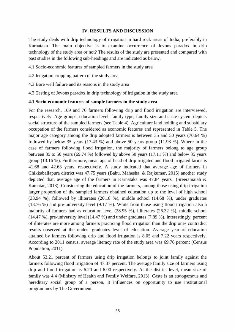
35
IV. RESULTS AND DISCUSSION
The study deals with drip technology of irrigation in hard rock areas of India, preferably in
Karnataka. The main objective is to examine occurrence of Jevons paradox in drip
technology of the study area or not? The results of the study are presented and compared with
past studies in the following sub-headings and are indicated as below.
4.1 Socio-economic features of sampled farmers in the study area
4.2 Irrigation cropping pattern of the study area
4.3 Bore well failure and its reasons in the study area
4.3 Testing of Jevons paradox in drip technology of irrigation in the study area
4.1 Socio-economic features of sample farmers in the study area
For the research, 109 and 76 farmers following drip and flood irrigation are interviewed,
respectively. Age groups, education level, family type, family size and caste system depicts
social structure of the sampled farmers (see Table 4). Agriculture land holding and subsidiary
occupation of the farmers considered as economic features and represented in Table 5. The
major age category among the drip adopted farmers is between 35 and 50 years (70.64 %)
followed by below 35 years (17.43 %) and above 50 years group (11.93 %). Where in the
case of farmers following flood irrigation, the majority of farmers belong to age group
between 35 to 50 years (69.74 %) followed by above 50 years (17.11 %) and below 35 years
group (13.16 %). Furthermore, mean age of head of drip irrigated and flood irrigated farms is
41.68 and 42.63 years, respectively. A study indicated that average age of farmers in
Chikkaballapura district was 47.75 years (Babu, Mahesha, & Rajkumar, 2015) another study
depicted that, average age of the farmers in Karnataka was 47.84 years (Sreeramaiah &
Kamatar, 2013). Considering the education of the farmers, among those using drip irrigation
larger proportion of the sampled farmers obtained education up to the level of high school
(33.94 %); followed by illiterates (20.18 %), middle school (14.68 %), under graduates
(13.76 %) and pre-university level (9.17 %). While from those using flood irrigation also a
majority of farmers had as education level (28.95 %), illiterates (26.32 %), middle school
(14.47 %), pre-university level (14.47 %) and under graduates (7.89 %). Interestingly, percent
of illiterates are more among farmers practicing flood irrigation than the drip ones contradict
results observed at the under -graduates level of education. Average year of education
attained by farmers following drip and flood irrigation is 8.05 and 7.22 years respectively.
According to 2011 census, average literacy rate of the study area was 69.76 percent (Census
Population, 2011).
About 53.21 percent of farmers using drip irrigation belongs to joint family against the
farmers following flood irrigation of 47.37 percent. The average family size of farmers using
drip and flood irrigation is 6.20 and 6.00 respectively. At the district level, mean size of
family was 4.4 (Ministry of Health and Family Welfare, 2013). Caste is an endogamous and
hereditary social group of a person. It influences on opportunity to use institutional
programmes by The Government.
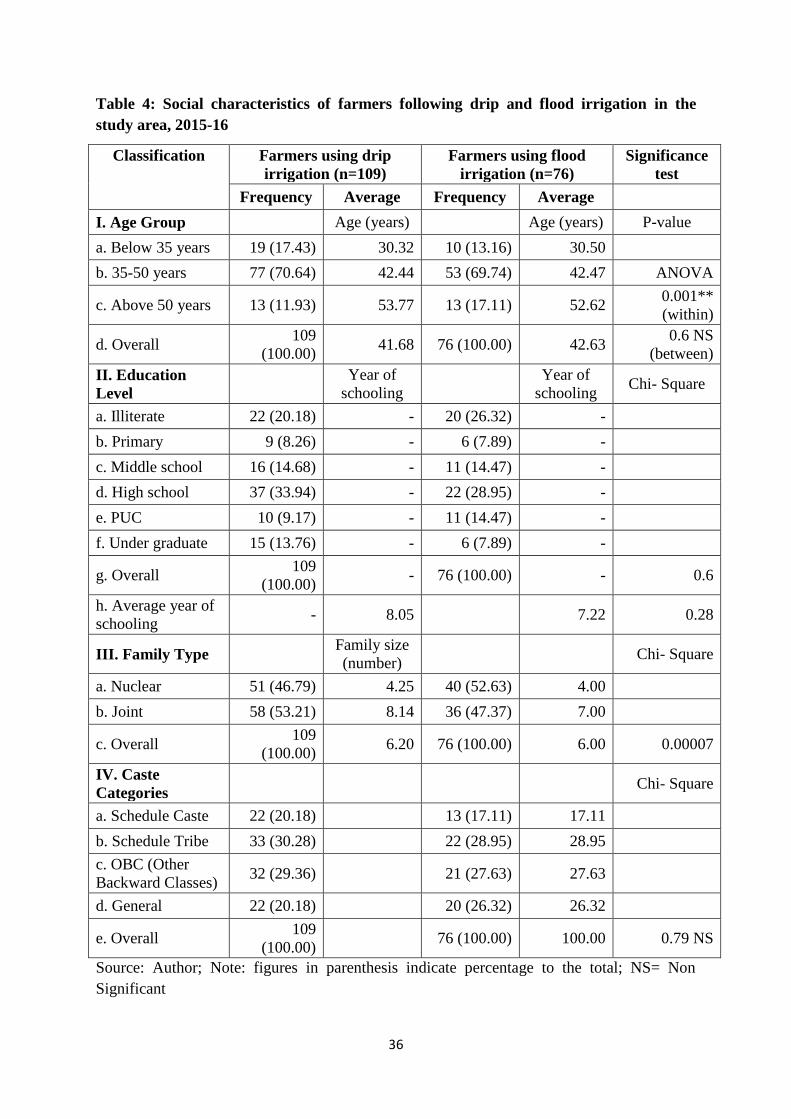
36
Table 4: Social characteristics of farmers following drip and flood irrigation in the
study area, 2015-16
Classification Farmers using drip
irrigation (n=109)
Farmers using flood
irrigation (n=76)
Significance
test
Frequency Average Frequency Average
I. Age Group Age (years) Age (years) P-value
a. Below 35 years 19 (17.43) 30.32 10 (13.16) 30.50
b. 35-50 years 77 (70.64) 42.44 53 (69.74) 42.47 ANOVA
c. Above 50 years 13 (11.93) 53.77 13 (17.11) 52.62 0.001**
(within)
d. Overall 109
(100.00) 41.68 76 (100.00) 42.63
0.6 NS
(between)
II. Education
Level
Year of
schooling
Year of
schooling Chi- Square
a. Illiterate 22 (20.18) - 20 (26.32) -
b. Primary 9 (8.26) - 6 (7.89) -
c. Middle school 16 (14.68) - 11 (14.47) -
d. High school 37 (33.94) - 22 (28.95) -
e. PUC 10 (9.17) - 11 (14.47) -
f. Under graduate 15 (13.76) - 6 (7.89) -
g. Overall 109
(100.00) - 76 (100.00) - 0.6
h. Average year of
schooling - 8.05 7.22 0.28
III. Family Type Family size
(number) Chi- Square
a. Nuclear 51 (46.79) 4.25 40 (52.63) 4.00
b. Joint 58 (53.21) 8.14 36 (47.37) 7.00
c. Overall 109
(100.00) 6.20 76 (100.00) 6.00 0.00007
IV. Caste
Categories Chi- Square
a. Schedule Caste 22 (20.18) 13 (17.11) 17.11
b. Schedule Tribe 33 (30.28) 22 (28.95) 28.95
c. OBC (Other
Backward Classes) 32 (29.36) 21 (27.63) 27.63
d. General 22 (20.18) 20 (26.32) 26.32
e. Overall 109
(100.00) 76 (100.00) 100.00 0.79 NS
Source: Author; Note: figures in parenthesis indicate percentage to the total; NS= Non
Significant

37
However, debate of equality among all caste groups is an ongoing issue in India. In the case
of drip, the majority of farmers belong to schedule tribe (30.28 %), followed by Other
Backward Class (OBC) (29.36 %) and each of schedule caste and general category shares
20.18 percent. Consider flood irrigation, similar pattern follow except general and scheduled
caste shares 26.32 and 17.11 percent respectively. The district census statistics of the study
area indicates that schedule caste and schedule tribe shares 24.9 and 12.5 percent respectively
(Census of India, 2011).
Among sampled farmers, the major share is by marginal farmers (farm size <1 ha) followed
by small farmers (farm size between 1 and 2 ha) and semi-medium farmers (farm size >2 ha).
Table 5: Economic characteristics of farmers following drip and flood irrigation in the
study area, 2015-16
Classification
Farmers using drip
irrigation
Farmers using drip
irrigation
Significance
test
Frequency Average Frequency Average P- value
I. Land holding Land holding
(ha)
Land holding
(ha)
a. Land holdings <
1ha 58 (53.21)
0.76 44 (57.89)
0.76
b. Land holding 1 to 2
ha 38 (34.86)
1.49 30 (39.47)
1.25 ANOVA
c. Land holding >2 ha 13 (11.93) 2.18
2 (2.63) 2.15
0.008
(within)
d. Overall 109
(100.00) 2.97
76 (100.00) 2.48
0.33
(between)
f. Rainfed land
holding 66 (60.55)
0.60 42 (55.26)
0.44 0.03 (within)
g. Irrigation land
holding size -
2.38 -
2.04 0.21
(between)
V. Subsidiary
occupation Chi- Square
a. Livestock activities 89 (81.65) - 50 (65.79) -
b. Self-employment
(shop, auto) 7 (6.42) - 8 (10.53) -
c. Wages and salary
(includes private,
government and
agriculture labour)
2 (1.83) - 4 (5.26) -
d. Not working 11 (10.09) - 14 (18.42) -
e. Overall 109
(100.00) - 76 (100.00) - 0.09
Source: Author; Note: figures in parenthesis indicate percentage to the total.
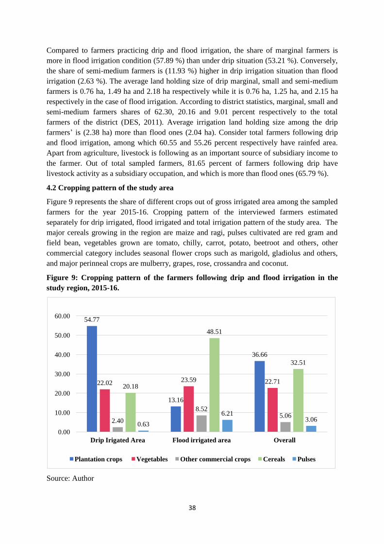
38
Compared to farmers practicing drip and flood irrigation, the share of marginal farmers is
more in flood irrigation condition (57.89 %) than under drip situation (53.21 %). Conversely,
the share of semi-medium farmers is (11.93 %) higher in drip irrigation situation than flood
irrigation (2.63 %). The average land holding size of drip marginal, small and semi-medium
farmers is 0.76 ha, 1.49 ha and 2.18 ha respectively while it is 0.76 ha, 1.25 ha, and 2.15 ha
respectively in the case of flood irrigation. According to district statistics, marginal, small and
semi-medium farmers shares of 62.30, 20.16 and 9.01 percent respectively to the total
farmers of the district (DES, 2011). Average irrigation land holding size among the drip
farmers’ is (2.38 ha) more than flood ones (2.04 ha). Consider total farmers following drip
and flood irrigation, among which 60.55 and 55.26 percent respectively have rainfed area.
Apart from agriculture, livestock is following as an important source of subsidiary income to
the farmer. Out of total sampled farmers, 81.65 percent of farmers following drip have
livestock activity as a subsidiary occupation, and which is more than flood ones (65.79 %).
4.2 Cropping pattern of the study area
Figure 9 represents the share of different crops out of gross irrigated area among the sampled
farmers for the year 2015-16. Cropping pattern of the interviewed farmers estimated
separately for drip irrigated, flood irrigated and total irrigation pattern of the study area. The
major cereals growing in the region are maize and ragi, pulses cultivated are red gram and
field bean, vegetables grown are tomato, chilly, carrot, potato, beetroot and others, other
commercial category includes seasonal flower crops such as marigold, gladiolus and others,
and major perinneal crops are mulberry, grapes, rose, crossandra and coconut.
Figure 9: Cropping pattern of the farmers following drip and flood irrigation in the
study region, 2015-16.
Source: Author
54.77
13.16
36.66
22.02 23.59 22.71
2.40
8.52 5.06
20.18
48.51
32.51
0.63
6.21 3.06
0.00
10.00
20.00
30.00
40.00
50.00
60.00
Drip Irigated Area Flood irrigated area Overall
Plantation crops Vegetables Other commercial crops Cereals Pulses
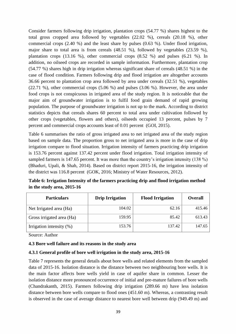
39
Consider farmers following drip irrigation, plantation crops (54.77 %) shares highest to the
total gross cropped area followed by vegetables (22.02 %), cereals (20.18 %), other
commercial crops (2.40 %) and the least share by pulses (0.63 %). Under flood irrigation,
major share to total area is from cereals (48.51 %), followed by vegetables (23.59 %),
plantation crops (13.16 %), other commercial crops (8.52 %) and pulses (6.21 %). In
addition, no oilseed crops are recorded in sample information. Furthermore, plantation crop
(54.77 %) shares high in drip irrigation whereas significant share of cereals (48.51 %) in the
case of flood condition. Farmers following drip and flood irrigation are altogether accounts
36.66 percent to plantation crop area followed by area under cereals (32.51 %), vegetables
(22.71 %), other commercial crops (5.06 %) and pulses (3.06 %). However, the area under
food crops is not conspicuous in irrigated area of the study region. It is noticeable that the
major aim of groundwater irrigation is to fulfil food grain demand of rapid growing
population. The purpose of groundwater irrigation is not up to the mark. According to district
statistics depicts that cereals shares 60 percent to total area under cultivation followed by
other crops (vegetables, flowers and others), oilseeds occupied 13 percent, pulses by 7
percent and commercial crops accounts least of 0.01 percent (GOI, 2015).
Table 6 summarises the ratio of gross irrigated area to net irrigated area of the study region
based on sample data. The proportion gross to net irrigated area is more in the case of drip
irrigation compare to flood situation. Irrigation intensity of farmers practicing drip irrigation
is 153.76 percent against 137.42 percent under flood irrigation. Total irrigation intensity of
sampled farmers is 147.65 percent. It was more than the country’s irrigation intensity (138 %)
(Bhaduri, Upali, & Shah, 2014). Based on district report 2015-16, the irrigation intensity of
the district was 116.8 percent (GOK, 2016; Ministry of Water Resources, 2012).
Table 6: Irrigation Intensity of the farmers practicing drip and flood irrigation method
in the study area, 2015-16
Particulars Drip Irrigation Flood Irrigation Overall
Net Irrigated area (Ha) 104.02 62.16 415.46
Gross irrigated area (Ha) 159.95 85.42 613.43
Irrigation intensity (%) 153.76 137.42 147.65
Source: Author
4.3 Bore well failure and its reasons in the study area
4.3.1 General profile of bore well irrigation in the study area, 2015-16
Table 7 represents the general details about bore wells and related elements from the sampled
data of 2015-16. Isolation distance is the distance between two neighbouring bore wells. It is
the main factor affects bore wells yield in case of aquifer share in common. Lesser the
isolation distance more pronounced occurrence of initial and pre-mature failures of bore wells
(Chandrakanth, 2015). Farmers following drip irrigation (289.66 m) have less isolation
distance between bore wells compare to flood ones (451.60 m). Whereas, a contrasting result
is observed in the case of average distance to nearest bore well between drip (949.49 m) and

40
flood irrigation farmers (1021.93 m). In addition, t-test result indicates that no significance
difference between farmers following drip and flood irrigations with respect to isolation
distance and distance to nearest water source. Mean drilling depth of bore well of farmers
following drip irrigation is 843.38 feet against 784.95 feet under flood irrigation. There is no
statistical significant difference between two groups (t-statistic 1.58, P < 0.05). A study
indicated that due to over-exploitation of the groundwater resource led to rapid growth of
shallow and deep bore wells and deep drilling decreases the life of the bore well (Nagaraj,
Marshal, & Sampath, 1999). Another work indicated that deepened drilling increases the cost
of drilling and probability of well failure (Bassi, Vijayshankar, & Kumar, 2008). The district
groundwater development level (141 %) alarmed the groundwater resource over exploitation.
The results of the study narrate that high horse power pump used by farmers following drip
irrigation (14.16 hp) compare to the flood irrigation (13.66 hp). Horse power of the pump
used to lift the water from the bore well is directly proportional to the depth of bore well
(FAO, 2007). Mean well yield of the tube well is 1.50 inch (1500 GPH) in drip irrigation
while it was 1.62 inch under flood irrigation (1620 GPH). The deviation of well yield
between drip and flood is statistically significant at 10 percent. According to district
groundwater information booklet of 2012 reported that average well yield in the district
varies between 0.5 to 20 m3
per hour (Ministry of Water Resources, 2012). Whereas, decline
in water yield of the bore well was observed and 57 percent of the various regions of the
country showed this trend between 2003-13 (CGWB, 2014).
Table 7: Bore well profile of the study area
Particulars
Farmers
following drip
irrigation
Farmers
following
flood
irrigation
T-test
Average isolation distance between two bore well
(m) 289.66 451.60 -1.16 NS
Average distance from bore well to nearest water
source (m) 949.49 1021.93 -0.70 NS
Average drilling depth of bore well (feet) 843.38 784.95 1.58 NS
Average power of pump used (HP) 14.16 13.66 0.70 NS
Average bore well yield (inch) 1.50 1.62 -1.89*
Average age of the bore well (years) 7.57 8.72 -1.65*
Average number of functional borewells 1.50 1.40 1.60 NS
Average number of failures at drilling 2.69 1.82 4.26***
Mean annual cost of repairs and maintenance per
borewell (INR) 15973.68 13298.11 2.39***
Source: Author; Note: *** significant < 1 percent; * significant < 10 percent; NS- non-
significant.
Mean age of bore well is 7.57 years under drip irrigation against the 8.72 years in the case of
flood situation. The mean difference is statistically significant at 10 percent. A study reported

41
that since after the green revolution average life of a borewell was less than 8 years while was
more twenty years before the revolution (Nagaraj, Chandrakanth, & Gurumurthy, 1994) .
Farmers used to have more than one borewell in order to fulfil the water requirement of crops
all around the year. The average number of functional bore wells under drip irrigation are
1.50 whereas 1.40 in flood irrigation. Average number of failed drillings under drip is 2.69
compared to 1.82 failures under flood irrigation and it is significant at 1 percent. Farmers
have to spend a certain amount per year for renewing pump oil and other costs on repairs if
any. Mean annual repair and maintenance cost of bore well is INR 15973.68 in the case of
farmers following drip irrigation against INR 13298.11 under flood irrigation and the mean
difference is significant at 1 percent. A study indicates that cost of maintainace and repairs
increases with depth of well drilling (Bassi, Vijayshankar, & Kumar, 2008).
4.3.2 Probability of bore well failure in the study area
Figure 10 indicates the proportion of farmers faced number of well failures in order to get a
success in the study region. In the case of drip irrigation, the number of bore well failures
ranges from 0 to 6 to get one successful bore well. Whereas, it varies from 1 to 5 under flood
irrigation. The majority of farmers practicing drip irrigation (29.36 %) get a successful bore
well at first attempt, followed by success at the cost of 1 drilling (25.69 %), after two failures
(18.35 %) and a success at fourth drilling (11.93 %). Whereas, the share of famers being
successful after 4 drilling (6.42 %), 6 failures (4.59 %) and 5 failures (3.67 %) is less than 15
percent of the total. Consider the flood irrigation, the highest number of farmers (34.21 %)
belongs to the category of getting successful well at the first drilling followed by success at
the cost of one drilling (21.05 %), success at third drilling (19.74 %), after 3 failures (14.47
%) and after 4 drillings (3.95 %) and at the six failures shares (6.58 %).
Figure 10: Frequency distribution of well failure to get a success among farmers
following drip and flood irrigation in the study area
Source: Author
29.36
25.69
18.35
11.93
6.42
3.67
4.59
34.21
21.05
19.74
14.47
3.95
6.58
0.00
0.00 5.00 10.00 15.00 20.00 25.00 30.00 35.00 40.00
0
1
2
3
4
5
6
Farmers following flood irrigation Farmers following drip irrigation
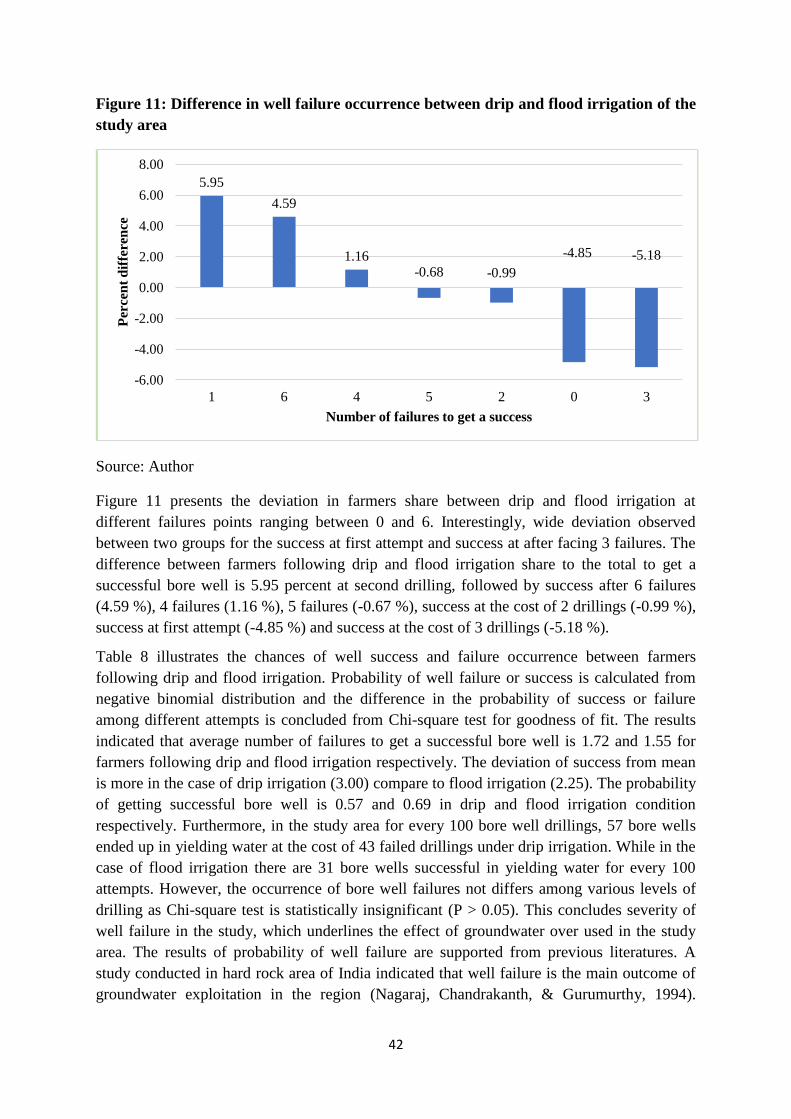
42
Figure 11: Difference in well failure occurrence between drip and flood irrigation of the
study area
Source: Author
Figure 11 presents the deviation in farmers share between drip and flood irrigation at
different failures points ranging between 0 and 6. Interestingly, wide deviation observed
between two groups for the success at first attempt and success at after facing 3 failures. The
difference between farmers following drip and flood irrigation share to the total to get a
successful bore well is 5.95 percent at second drilling, followed by success after 6 failures
(4.59 %), 4 failures (1.16 %), 5 failures (-0.67 %), success at the cost of 2 drillings (-0.99 %),
success at first attempt (-4.85 %) and success at the cost of 3 drillings (-5.18 %).
Table 8 illustrates the chances of well success and failure occurrence between farmers
following drip and flood irrigation. Probability of well failure or success is calculated from
negative binomial distribution and the difference in the probability of success or failure
among different attempts is concluded from Chi-square test for goodness of fit. The results
indicated that average number of failures to get a successful bore well is 1.72 and 1.55 for
farmers following drip and flood irrigation respectively. The deviation of success from mean
is more in the case of drip irrigation (3.00) compare to flood irrigation (2.25). The probability
of getting successful bore well is 0.57 and 0.69 in drip and flood irrigation condition
respectively. Furthermore, in the study area for every 100 bore well drillings, 57 bore wells
ended up in yielding water at the cost of 43 failed drillings under drip irrigation. While in the
case of flood irrigation there are 31 bore wells successful in yielding water for every 100
attempts. However, the occurrence of bore well failures not differs among various levels of
drilling as Chi-square test is statistically insignificant (P > 0.05). This concludes severity of
well failure in the study, which underlines the effect of groundwater over used in the study
area. The results of probability of well failure are supported from previous literatures. A
study conducted in hard rock area of India indicated that well failure is the main outcome of
groundwater exploitation in the region (Nagaraj, Chandrakanth, & Gurumurthy, 1994).
5.95
4.59
1.16 -0.68 -0.99
-4.85 -5.18
-6.00
-4.00
-2.00
0.00
2.00
4.00
6.00
8.00
1 6 4 5 2 0 3
Per
cen
t d
iffe
ren
ce
Number of failures to get a success
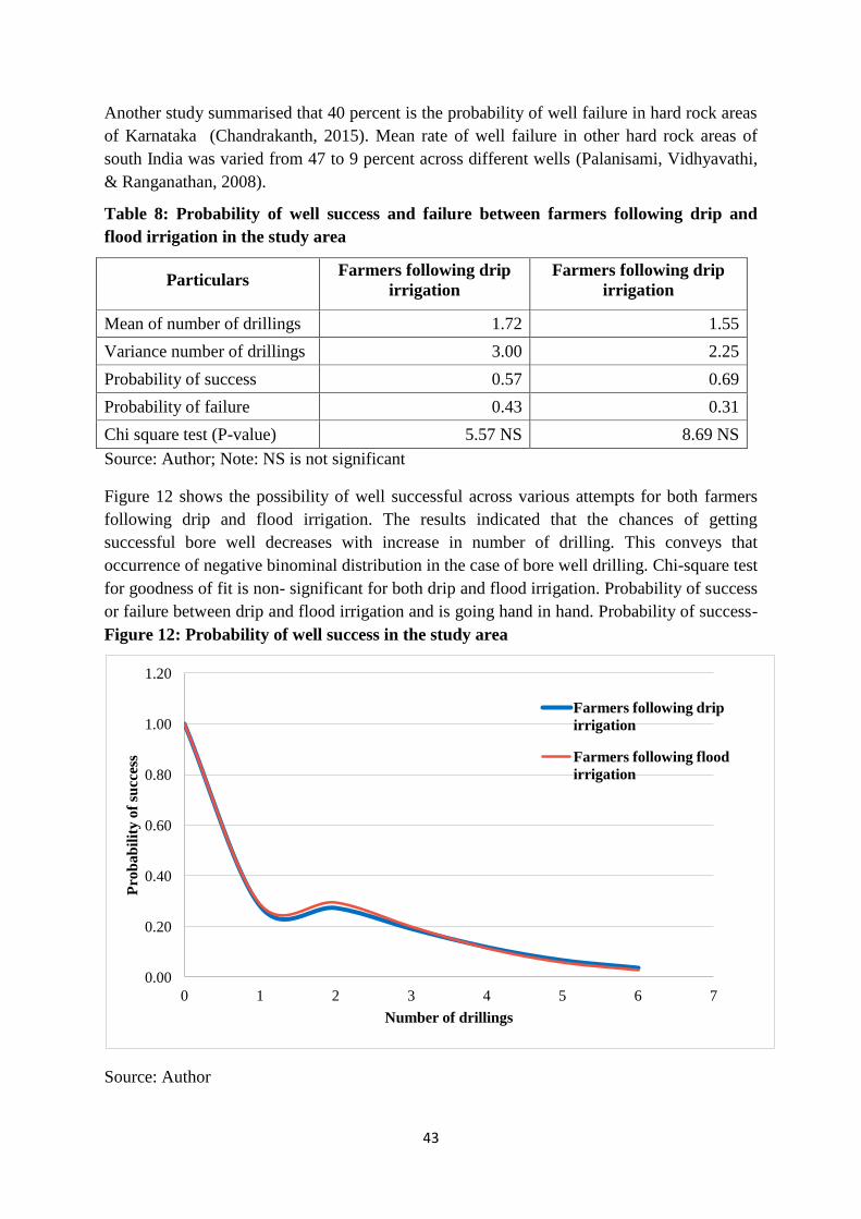
43
Another study summarised that 40 percent is the probability of well failure in hard rock areas
of Karnataka (Chandrakanth, 2015). Mean rate of well failure in other hard rock areas of
south India was varied from 47 to 9 percent across different wells (Palanisami, Vidhyavathi,
& Ranganathan, 2008).
Table 8: Probability of well success and failure between farmers following drip and
flood irrigation in the study area
Particulars Farmers following drip
irrigation
Farmers following drip
irrigation
Mean of number of drillings 1.72 1.55
Variance number of drillings 3.00 2.25
Probability of success 0.57 0.69
Probability of failure 0.43 0.31
Chi square test (P-value) 5.57 NS 8.69 NS
Source: Author; Note: NS is not significant
Figure 12 shows the possibility of well successful across various attempts for both farmers
following drip and flood irrigation. The results indicated that the chances of getting
successful bore well decreases with increase in number of drilling. This conveys that
occurrence of negative binominal distribution in the case of bore well drilling. Chi-square test
for goodness of fit is non- significant for both drip and flood irrigation. Probability of success
or failure between drip and flood irrigation and is going hand in hand. Probability of success-
Figure 12: Probability of well success in the study area
Source: Author
0.00
0.20
0.40
0.60
0.80
1.00
1.20
0 1 2 3 4 5 6 7
Pro
bab
ilit
y o
f su
cces
s
Number of drillings
Farmers following drip
irrigation
Farmers following flood
irrigation

44
-varies from 1 to 0.03 for farmers practicing drip and flood irrigation for different number of
attempts, respectively. The probability of well failure is more under drip irrigation than flood
condition. Therefore, the first research null hypothesis that tube well failures same in both
drip and flood irrigation is dropped and alternative hypothesis is accepted. It concludes the
severity of groundwater overused in the study area.
4.3.3 Reasons for bore well failure in the study area
Table 9 describes the causes of groundwater depletion in the study area from the primary
interview from the farmers following irrigation. Based on the sampled data analysis, out of
total sample 80.54 percent of farmers expected that a decrease in the quantum rainfall is the
main reason for groundwater depletion followed by wells with no specific isolation distances
(63.24 %), regular cut of electricity (62.70 %), tanks without proper de-siltation (59.46 %),
irrigation tanks with irregular fill (55.68 %), cultivation of water demanding crops (49.19 %),
adoption of high power submersible and electric pumps (40.54 %), tube well location is out
of command area (37.30 %), drilling at out of point located by local diviner (36.76 %), and
drilling point was excluded from Geologist indication (28.11 %).
Interestingly, no one responded on supply side elements of groundwater such as groundwater
recharge efforts from them, water conservation structures such as farm pond, rainwater
harvesting and other water conservation practices in the farm. However, there are cultivation
practices to conserve water namely mulching, zero tillage, use of anti-transparent. Also, self
responsibility in reducing unnecessary water losses in public or private places and other
practices.
Table 9: Reasons for bore well failure in the study area in 2015-16
Sl. No. Reasons Percent of respondents
(Total respondents 185)
1 Decreasing quantum of rainfall 80.54
2 Densely spaced wells 63.24
3 Frequent power cuts/load shedding 62.70
4 Tanks not desilted-poor groundwater recharge 59.46
5 Irrigation tanks are not regularly filled up 55.68
6 Water Intensive crops 49.19
7 Use of high HP pumps 40.54
8 Well is located outside the command area 37.30
9 Did not drilled at the point shown by local diviner 36.76
10 Did not drilled at the point shown by Geologist 28.11
Source: Author
Therefore, it represents the lack of self-responsibility from farmers’ side in water
conservation, on the other hand it also shows farmers still has to realise the importance of
water for now and in concern to future generation. A study results indicated that extensive
pumping of water to grow profitable crops led to groundwater overuse (Sandra, 2015).

45
Another study concluded that increases in importance to groundwater irrigation to fulfil food
demand of rapid growing population (Braun, Ashok, & Peter, Indian Agriculture and Rural
Development: Strategic Issues and Reform Options, 2005). Stabilized water supply is
essential for the potential use of inputs such as seed, labour, fertilizers and others. In addition,
requirement of large investment for canal irrigation lead to broaden the scope for
groundwater irrigation (Anik, Upali, & Tushaar, 2014). This, demand side interests neglect
the supply side elements of groundwater resources. Furthermore, it ended up in overuse of
groundwater in many parts of India and the study area is not an exceptional from this.
4.4 Testing of Jevons paradox in drip technology of irrigation in the study area
4.4.1 Estimation of probit model
Table 10 summarises the first part of 2SLS estimation for instrumental variables selection.
The findings depicts that caste categories and distance to loan institution made significant
effect on loan amount borrowed by the farmers at 1 percent significance level. It also
explained by farm size, percentage of area under perinneal crops, crop type (plantation=1,
seasonal=0), mean distance to nearest water source from farmer’s bore well, total distance to
product market significantly at 5 percent level of significance. Whereas, the mean power of
pump used to lift groundwater affected significantly at 10 percent level. The model is
significant according to Wald test of exogeneity as chi square test is significant (P <0.05).
This validates the use of instrumental variables distance to loan institution and total distance
to product markets for the loan amount borrowed by farmers from bank/s. in addition,
distance to loan institution/s and total distance to product markets are correlated with the loan
amount borrowed by the farmer. It depicts the relevance of these variables with the loan
amount borrowed. Therefore, total distance to market and distance to loan institution selected
as instrumental variables as other variables are in the main equation to assess the
determinants of drip adoption.
In the situations, distance to loan institution from farmer’s village is an important variable
which decides the easiness of credit access. Easier the access more will be the transactions
with the bank, increases the financial inclusion and help to create good relationship with
bank, to update knowledge about bank services, Governmental programmes. Thus, distance
to loan institution/s explains the total amount borrowed by farmer. Furthermore, it is not
related with other factors, which determines the drip implementation by the farmers.
Therefore, it is uncorrelated with other independent variables included in the model and error
term of omitted variables of model. Another one more important variable which explains loan
amount borrowed is the total distance to product market from farmer’s village. The lesser
distance to product market, increases the marketing opportunities. It also reduces the
transportation cost, greater accessibility to inputs, it guides the best crop choice, wider
choices of crops to cultivate, more preferably perishables such as vegetables, fruits, flowers
and other commercial crops. For such crops farmers need to investment on inputs such as
seeds, fertilizers, labour, green house structures which will lead to borrow loans from banks.
However, lesser distance to product markets also increases the financial liquidity of the
farmers which may reduces the dependency on loan amount. Nonetheless investment on
inputs is the initial cause for the further earnings from the crop cultivation. Moreover,

46
irrigation and land development infrastructures are the base for wider crop choices, which
requires long term investment.
Table 10: Estimates of endogenous variable with instrumental and other independent
variables of drip adoption in the study area.
Sl. No. Independent variable - loan amount of the farmers with the bank/s (in INR)
1 Dependent variables Coefficient
2 Farm size 13380.57**
3 % of plantation area 849.2594**
4 Crop type (Seasonal=0, Perinneal=1) -55915.78**
5 Age 1395.421
6 Family size -2223.864
7 Average power of pump used to lift groundwater -2068.109*
8 Average distance between two neighbouring bore wells -20.82957
9 Average distance to the nearest water source from farmer’s bore
well -19.50998**
10 Number of milk yielding animals 5735.854
11 d1 caste (Scheduled tribe) 54098.11**
12 d2_caste (Other backward classes) 58514.52***
13 d3 caste (General) 105838.5**
14 Years of education received 6360.721***
15 Years of education received * d1 caste -4439.619
16 Years of education received * d2 caste -4291.399
17 Years of education received * d3 caste -10254.6**
18 Distance to loan institution 4444.527***
19 Total distance to product market -234.4584**
20 Intercept -39138.87
21 Athrho -1.29069
22 Insigma 11.2925
23 Wald test of exogeneity 10.57
24 Prob> chi2 0.0011
Source: Author; Note: *** < 0.01 significance level and ** <0.05 significance level
Secondly, Table 11 shows the results of the probit for drip technology (farmers following
drip=1, farmers following flood= 0) by linear probit model of 2SLS. The model significant as
Chi-square test probability is less than 0.05 P-value. The results showed that loan amount
borrowed from banks made high significant effect on farmer’s action for drip technology
adoption. In detail, probability of drip adoption will increases by 0.00123 percent for every-
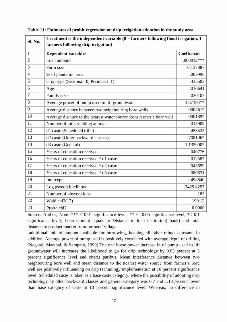
47
Table 11: Estimates of probit regression on drip irrigation adoption in the study area.
Sl. No. Treatment is the independent variable (0 = farmers following flood irrigation, 1
farmers following drip irrigation)
1 Dependent variables Coefficient
2 Loan amount .000012***
3 Farm size 0.137887
4 % of plantation area .003996
5 Crop type (Seasonal=0, Perinneal=1) .435503
6 Age -.016641
7 Family size .030107
8 Average power of pump used to lift groundwater .037194**
9 Average distance between two neighbouring bore wells .000461*
10 Average distance to the nearest water source from farmer’s bore well .000189*
11 Number of milk yielding animals .013909
12 d1 caste (Scheduled tribe) -.453525
13 d2 caste (Other backward classes) -.708106*
14 d3 caste (General) -1.135900*
15 Years of education received .040776
16 Years of education received * d1 caste .012587
17 Years of education received * d2 caste .043659
18 Years of education received * d3 caste .080631
19 Intercept -.498840
20 Log pseudo likelihood -2429.8297
21 Number of observations 185
22 Wald chi2(17) 199.12
23 Prob> chi2 0.0000
Source: Author; Note: *** < 0.01 significance level, ** < 0.05 significance level, *< 0.1
significance level; Loan amount equals to Distance to loan institution( bank) and total
distance to product market from farmers’ village
-additional unit of amount available for borrowing, keeping all other things constant. In
addition, Average power of pump used is positively correlated with average depth of drilling
(Nagaraj, Marshal, & Sampath, 1999).The one horse power increase in of pump used to lift
groundwater will increases the likelihood to go for drip technology by 0.03 percent at 5
percent significance level and citeris paribus. Mean interference distance between two
neighbouring bore well and mean distance to the nearest water source from farmer’s bore
well are positively influencing on drip technology implementation at 10 percent significance
level. Scheduled caste is taken as a base caste category, where the possibility of adopting drip
technology by other backward classes and general category was 0.7 and 1.13 percent lower
than base category of caste at 10 percent significance level. Whereas, no difference in

48
adoption of drip between scheduled class and scheduled tribe. This is because schedule caste
and schedule tribe are considered as the most disadvantaged social groups in India. Thus,
there are many Governmental programmes to support them economically such as
scholarships to students, reservation in education institutes and in government jobs, subsidy
to the initial investment such as drip adoption, green house construction, special assistance
through public distribution programmes and many other (Sekhri, 2011; Nair, 2017)While in
the case of other backward and general category people receives less institutional supports
than Scheduled Caste (SC) and Scheduled Tribes (ST). However, drip adoption is not
influenced by type of crop, area under plantation crops, farm size, family size, age of the
farmer and education of the farmer.
Some literature indicated that power of pump used to lift water, year of schooling,
dependency ratio (Namara, Nagar, & Upadhyay, 2007), age of farmer, farm size, wider crops
and non-farm income (Goyal, 2015) made a positive and significant effect on drip
technology adoption. But, area under cereals had a negative effect on drip technology
(Namara, Nagar, & Upadhyay, 2007). In addition, possibility of drip adoption increases with
increase in depth of bore well, higher share of fruits, vegetables, plantation crops more the
rate of adoption and socio-economic variables made and significant effect on drip technology
implementation (Regassa, Upadhyay, & Nagar, 2005). Furthermore, crop cultivation
elements, physical, socio-economical and financial variables decide the micro irrigation
implementation (Dhawan, 2000).
4.4.2 Propensity scores and average treatment estimation
Table 12 presents the distribution of propensity scores over 4 blocks namely 0.008, 0.2, 0.4,
0.6 and 0.8. In each block, certain units of controlled units (farmers practicing flood irrigated)
matched with treated units (farmers adopting drip irrigation). Propensity scores estimated
indicates the all the factors and elements considered during drip technology adoption. Thus, it
avoids the selection bias.
Table 12: Blocks/Cells for Treated and Control Groups to check balancing property
Sl No. Inferior of block of
propensity scores
Controlled
units Treated units Sub total
1 0.008 25 2 27
2 0.2 23 11 34
3 0.4 7 13 20
4 0.6 10 23 33
5 0.8 5 60 65
Grand total 70 109 179
Note: the common support option has been selected, Balancing property satisfied
In the matching, a treatment unit should be match with more than one controlled units.
However, one to one matching is preferred commonly as it is difficult find in real situation

49
(Glazerman, Levy, & Myers, 2003). The results indicate that range of controlled units
matched varies from five to 25 of each block, while it is between two and 60 among treated
units. Where in the case of total number of matched controlled units are 70 out of 76
observations with the 109 treated units. The total number of observation considered for
estimating propensity scores are 179.
Common support is the main assumption of propensity score matching i.e., certain number of
propensity scores of controlled units should be similar with the treated ones. It is difficult in
real condition but at least there must be some overlap between controlled and treated units
scores are preferable. Common support option has been selected in STATA software based
on the results obtained indicates that the balancing property of the score is satisfied. Figure 13
describes the distribution of propensity scores between controlled units (farmers following
flood irrigation = 0) and treated units (farmers adopting drip irrigation =1). Both histograms
indicate the region of overlap between farmers following drip and flood irrigation. Therefore,
the propensity scores are valid to estimate the average treatment effect of the drip technology
on groundwater use by the farmers.
Figure 13: Matching pattern between farmers practicing drip (treated) and flood
(control) irrigation in the study area.
Source: Author
Table 13 represents the average treatment effect on groundwater used by the famers for crop
cultivation. The results conclude that there is a significant difference between quantity of
water used between farmers practicing drip and flood irrigation to raise the crops. According
to radius matching, 62 of controlled units matched with 73 of treated units. The mean
difference in groundwater used is -6.715 acre-inch, in other words farmers adopting drip used
01
23
0 .5 1 0 .5 1
0 1
De
nsi
ty
Probability of positive outcomeGraphs by treatment

50
6.715 acre inch less groundwater than the farmers following conventional or flood irrigation
at 5 percent significance level. Considered kernel matching method, average difference of
groundwater used is -12.66 acre-inch. Mean difference summarised that farmers practicing
flood irrigation used 12.66 acre-inch of groundwater more than the farmers practicing drip
irrigation and it is significant at 5 percent level.
Table13: Average treatment effect based on different matching method
Matching method Matched
control
units
Matched
treated
units
ATT (Y1 –
Y0)
t-Statistic Confidence interval of
95 %
Radius 62 73 -6.715 -2.513 ** -12.724 to -0.618
Kernel 76 109 -12.666 -1.962** -39.317 to -4.461
Nearest
neighbourhood 28 109 -12.856 -1.838 * -44.424 to -5.028
Source: Author; Note: ** significance at< 5 percent; * significance at <10 percent
Where, the 76 units of controlled matched with 109 treated observations. The results of the
nearest neighbourhood type describes that average use of groundwater among treated group
(drip) is 12.856 acre inch lower than the controlled (flood) farmers at 10 percent significant
level with the matching of 28 units of controlled units with the 109 treated elements.
Finally, as per the results of radius and kernel matching the drip technology results in water
savings and it is in the way to serve its objective. Thus, there is no existence of rebound effect
or Jevons paradox in drip irrigation technology of the study area. Drip technology is in the
line of conservation of groundwater resources. Thus, the second research null hypothesis is
rejected and the alternative hypothesis that mean groundwater used in the case of drip is less
than flood irrigation. A study reported that drip and sprinkler irrigation will reduces the water
consumption under limitation of extension of area under irrigation (Berbel & Mateos, Does
investment in irrigation technology necessarily generate rebound effects? A simulation
analysis based on an agro-economic model, 2014). Another study in Spain showed that the
country saved 12 percent water from irrigation modernization (Loch & Adamson, 2015).
One more study in India also indicated that drip technology using less water than flood or
conventional irrigation system (Patil, Chandrakanth, Mahadev, & Manjunatha, 2015).
Even though there is no evidence of occurrence of Jevons or rebound effect in drip irrigation
technology. According to previous section results showed that there was no significance
difference in socio economic characteristics such as age, education, family size, land holding
and others between farmers following drip and flood irrigation. In addition, mean drilled
depth of bore well is more under drip than flood irrigation, average isolation distance
between two neighbouring bore well is less in drip against flood condition. In addition, bore
well yield is less in the case of farmers practicing drip than flood irrigation and statistically
significant. Mean number of failed drilling and repair and maintenance cost are significantly
more under drip than flood irrigation. Furthermore, intensity of well failure more in the case
of farmers following drip irrigation compared to flood ones. This illustrates that drip

51
irrigation can reduce the amount of water used for crop cultivation but is not only a sole
solution to conserve the groundwater resource. Thus, it is important to take key action in
other areas such as educating farmers regarding importance of water for future, conduct
trainings on groundwater recharge techniques such as rainwater harvesting, watershed
management and other elements. It is also need to make reach of real purpose of drip
technology i.e., it is to decrease water consumption not to increase area under irrigation or not
to gain profit to avoid occurrence of rebound effect in future. Some literature above indicated
that drip and sprinkler technology saves water only under the limitation on area under
irrigation (Berbel & Mateos, 2014). Thus, the institutional efforts are needed in this regard
without compromising food security of the country. It can be feasible to reallocate the drip
subsidy amount, considerably for drip irrigation on other hand for other groundwater
recharge and conservation programmes such as encouragement for zero tillage, rainwater
harvesting, on farm water reducing practices and other methods.

52
V CONCLUSION AND RECOMMENDATION
This chapter summarises and concludes the salient findings of the study on drip
irrigation technology in hard rock areas of India and testing of Jevons paradox in Karnataka,
India.
5.1 Introduction
Micro irrigation is a noticeable innovation in the field of irrigation. Preferably for the water
stressed and heavy populated countries such as India, China and other economies. However
the achievement of micro irrigation area in India is less compare to the rest of the world
namely Israel, USA, Spain, Russia and others. However, the continuous effort to promote
technologies is under process.
Overuse of groundwater has been rising as a challenging issue to the country with respect to
water management and food security. Groundwater depletion results in initial and pre- mature
failure of bore wells, deepened drillings coupled with installation of high powered pump to
lift water and increased in irrigation cost. Well failure is an important feature of groundwater
over exploitation in a region. Well failure is occurring in many parts of India, preferably in
hard rock areas of the country such as Karnataka, Tamil Nadu, Andhra Pradesh and others
parts. Thus, institutional efforts are framed to address groundwater depletion in concern of
the country’s future survival as water is an important constitute for life. One important among
those is encouragement to micro-irrigation technologies namely adoption of drip and
sprinkler irrigation. Micro-irrigation technology is an innovative method of supplying water
at the root zone of plant in the form of drop by drop. This pattern of irrigation reduces evapo-
transpiration losses, conveyance losses and other type of losses. Thus, efficiency of the
method is higher than the other conventional methods of irrigation such as flood irrigation,
ridge and furrow method, check and basin and many other methods. The main agenda of
micro irrigation is ‘more crops per drop’. In India, drip and sprinkler method has wider
adoption among various methods of micro irrigation. These methods do not only reducing
water consumption or increasing water use efficiency, but also lower labour requirement,
increases productivity and increases the net returns of the crop cultivation.
However, technology adoption and resource use efficiency have been subject for debate.
Technology not always opens a way to reduce resource consumption by enhancing resource
use efficiency. In detail, increase in resource use efficiency by technology, reduces the cost of
production, which in turn migh increases demand for the resource. It will end up in
consuming more units of the resources rather than conserving the resource. This is called as
the rebound effect or Jevons paradox in economics.
Therefore, present study aimed to assess whether the drip technology adoption in the study
area reduces the groundwater used for crop cultivation or it is ending up in increasing the
resource consumption.
Research objectives of the study:
1. To estimate the probability of well failure on farms with and without drip irrigation.

53
2. To test the hypothesis for Jevons paradox in drip irrigation technology of the study area.
5.2 Major findings of the study:
Consider Overall irrigation cropping pattern, the highest share in case of plantation
crops (36.66 %) followed by cereals (32.51 %), vegetables (22.71 %), other
commercial crops (5.06 %) and pulses (3.06 %) accounts least portion. It is noticeable
that share of food crops is insignificant.
It is noticeable that the share food crops is less under irrigation.
Irrigation cropping intensity of irrigated farmer’s is 147.65 percent. However, the
irrigation intensity of farmers following drip and flood irrigation is 153.76 and 137.42
percent, respectively. Thus, annual area cultivated is more under drip than under flood
irrigation.
Average number of functional bore wells is more under drip (1.50) irrigation than
flood (1.62) irrigation.
Mean number of failed drilling under drip and flood irrigation are 2.69 and 1.82
respectively. The difference is statistically significant at 1 percent.
Average annual cost of repairs and maintenance per bore well is INR 15973.68 in the
case of drip irrigation while it is INR 13298.11 under flood irrigation.
The mean number of drilling in the sampled farmers is higher in the case of drip
irrigation (1.72) compare to flood one (1.55). While contradict findings in the
variance of drilling between drip (3.00) and flood (2.25) situation. This satisfied the
unique feature (mean> variance) of negative binomial distribution.
The probability of well failure is 0.43 and 0.31 in the case of drip and flood irrigation
respectively.
Well failure results depicted that to get 100 successful bore well farmers has to
attempt 143 drillings under drip condition against 131 attempts under flood irrigation.
In addition, the drilling without yielding water are 43 and 31 under drip and flood
irrigation.
Furthermore, for every 100 drilling in the case of drip farmers will get 57 successful
bore wells while it is 69 in the case of flood irrigation.
The research first hypothesis is rejected and alternative hypothesis that the probability
of well failure high under drip irrigation than flood irrigation is accepted.
According farmers point of view, 80.54 percent out of total respondents expressed
that decreasing quantum of rainfall is the main reason for well failure followed by
densely spaced tubewells (63.24 %), frequent cut of electricity (62.70 %), improper de
silted tanks (59.46 %), irregular filled up of irrigation tanks (55.68 %), cultivation of
water intensive crops (49.19 %), use of high powered pump (40.54 %), location of
bore well outside command area (37.30 %), drilling at point indicated by local diviner
and deviation drilling point predicted by Geologist.
No farmer aware about their self-responsibility of groundwater recharge, reduced
water wastages in public and private places, lack of interest in water conservation
structures and other self responsibilities.
54
Estimation of probit model for drip technology adoption (drip = 1, flood = 0)
indicated that loan amount and average power of pump used to lift groundwater
explained drip implementation at 1 and 5 percent level of significance.
Increase in additional unit available of loan will going to increase possibility of
having drip irrigation by 0.0012 percent at 1 percent significance level and citeris
paribus. Similarly, one horse power increase in the pump used to lift water will
increases the chances of going for drip adoption by 0.03 percent at 5 percent level of
significance and keeping all other thing constant.
Average interference distance between two neighbouring bore well and mean distance
to the nearest water source from farmer’s bore well are positively influencing on drip
technology implementation at 10 percent significance level.
Scheduled class is the base caste category, the possibility of drip adoption by other
backward classes and general category was 0.7 and 1.13 percent lower than base
category at 10 percent significance level and citeris paribus. However, no difference
in adoption between scheduled class and scheduled tribe. Where the caste reservation
is the ongoing debate subject in the country.
Type of crop, area under plantation crops, farm size, farmer’s age and education of
the farmer have no influence on drip implementation.
The propensity scores blocks are divided into five, each block has certain
observations in both control and treated groups. Thus, balancing property of the
scores satisfied.
According to radius matching, 62 controlled and 73 treated observations are matched.
Mean use of groundwater in drip irrigation is 6.715acre-inch less than flood condition.
In kernel matching, 76 farmers following flood irrigation matched with 109 drip ones.
Average consumption of groundwater for crop cultivation in drip irrigation is
12.66acre-inch less than flood situation.
As per nearest neighbour method, 28 controlled farmers matched with 109 drip ones.
Mean groundwater used for crop grown in flood irrigation is 12.856 acre-inch more
than drip condition.
Thus, the research second objective mean groundwater used for crop cultivation same
under drip and flood irrigation was rejected and accepted the alternative hypothesis.
5.3 Recommendations:
More than 50 percent of the sampled farmers are illiterate and received just up to
primary school education and belongs to age group between 35 and 50. It necessitates
to enhance farmer’s knowledge with regard to current issues, agricultural
technologies, agriculture marketing opportunities, input and output prices. It is
necessary to arrange educational programmes such as farm schools, arranging
motivational agriculture dramas during off seasons, interaction sessions with
agriculture scientists and farmers and other agricultural events.
The main agenda of groundwater irrigation is to fulfil the demand of food grain
production. However, area under food crops is not appreciable under irrigation among
the sampled farmers. Although vegetables accounts more than 20 percent. Therefore,
55
there is a need to reallocate the area to different types of crops substantially. The
policies to address sustainable cropping pattern in the region are essential.
Well failure is the major problem in the study and indicated that 43 and 31 percent of
well failure under drip and flood irrigation, respectively. It depicts that groundwater
overuse in the area. Though the farmers expressed the reasons for the well failure only
on demand side such as reduced rainfall amount, densely spaced wells, improper
electricity supply, tanks with improper de siltation and others. However, farmers fail
to recognise their responsibilities such as groundwater recharge, rainwater harvesting,
cutting of unnecessary water loss in the area and other farmers’ initiations. Thus, it is
important to create cognizance about water conservation among farmers. Designing of
group discussions, campaign, and scene plays on water crisis and water management
practices.
It is worthful to take up in depth research in the study regarding water usage for
different purposes in households, local water supply system, assessment of people
concern to water wastage, ways to figure out water conservation in the study.
Caste is playing a significant role to some extent in adoption of drip irrigation
technology. It can create inequality in the social system and evades people to go for
technology implementation by social structure. It is important to provide more
opportunities to disadvantaged group than others. But, economic and financial
condition is the better way of measure one’s social disadvantage status rather than
caste. It is important to target the right group at right amount of institutional supports.
Therefore, restructuring of Government support schemes such as educational
opportunities, credit availability, subsidy for drip, easy access to bank services by
considering income level as a base to afford in the study area.
The study proved that drip irrigation is reducing the water consumption for crop
cultivation compare to flood or conventional irrigation. In concern to future
sustainability of the technology, it is necessary to limit the area under irrigation in the
study area as the area cropping intensity under drip more than flood irrigation.
Meanwhile, it is important to taken care of food security.
Though drip irrigation is saving water in the study, area under irrigation is more for
plantation, vegetable and commercial crops than food crops. Indicated that the
farmers in the study area accepted technology as profitable instrument rather than
water conservation tool. It is essential to make reach of drip technology goal to end
users (farmers). Thus, necessary to organise extension training programmes to farmers
for reaching the drip technology main objective and reason for providing subsidies is
to conserve water not to increase farmer’s profit in the study area.
Although drip irrigation reduces water consumption but is not only enough to evade
groundwater exploitation in the study area. Thus, it is feasible to reframe policies to
encourage farmers in rainwater harvesting, water reduction practices such as zero
tillage, mulching, anti-transparents use. For example providing direct payment for the
farmers, who following certain fixed area under zero tillage or giving subsidies to
anti-transparents. Also give a target amount of water to be saved per village by
offering incentives, which motivates the water conservation of the community. It not
only increases water saving and also builds social capital in the area.
56
VI REFERENCES
Alain, A. (2004). Economics. Navarra, Spain: Causeway Press.
Alcott, B. (2015). Jevons' Paradox. Ecological Economics , 9-21.
Alferd, D. (1891, February 9). Trove . Retrieved March 30, 2017, from National Library of
Australia Web Site: https://trove.nla.gov.au/newspaper/article/26771520
Amarendra, P. S., & Narayanan, K. (2013, January 17). Special Research Netwrok. Retrieved
March 30, 2017, from Special Research Netwrok Web Site:
https://papers.ssrn.com/sol3/papers.cfm?abstract_id=2202053
Anantha, K. H., & Raju, K. V. (2008). Groundwater Over-Exploitation, Costs and Adoption
Measures in the Central Dry Zone of Karnataka. Bangalore: Institute for Social and
Economic Change.
Austin, P. C. (2011). An Introduction to Propensity Score Methods for Reducing the Effects
of Confounding in Observational Studies. Multivariate Behavioral Research , 322-424.
Babu, P. B., Mahesha, M., & Rajkumar, B. J. (2015). Utilization of Benefits from
Government Programmes by Irrigated and Rainfed Farmers in Chikkaballapura District of
Karnataka- an Comparative Analysis. International Journal of Agricultural Science and
Research , 173-182.
Balyan, S. K. (2016). Accelerating growth of Indian agriculture: Micro irrigation an efficient
solution. New Delhi: Ministery of State and Farmers Welfare.
Bassi, N., Vijayshankar, P., & Kumar, D. M. (2008). Wells and Ill-fare: Impacts of Well
Failures on Cultivators in Hard Rock Areas of Madhya Pradesh. Proceedings of the 7th
Annual Partners Meet (pp. 310-330). Hyderabad: International Water Management Institute.
Berbel, J., & Mateos, L. (2014). Does investment in irrigation technology necessarily
generate rebound effects? A simulation analysis based on an agro-economic model.
Agricultural Systems , 25-34.
Bhaduri, A., Upali, A., & Shah, T. (2014, November 14). Groundwater Irrigation Expansion
in India:An Analysis and Prognosis. Retrieved March 21, 2017, from
http://publications.iwmi.org: http://publications.iwmi.org/pdf/H039616.pdf
Bhende, M. J. (2013, August). Institute for Social and Economic Change. Retrieved March
20, 2017, from Institute for Social and Economic Change Web Site:
http://www.isec.ac.in/Agri%20Profile-Karnataka.pdf
Braun, V. J., Gulati, A., & Hazzel, P. (2005). Indian Agriculture and Rural Development:
Strategic Issues and Reform Options. Washington D.C.: Intenational Food Policy Research.
Carmen, R. (2000, October). World Resources Institute. Retrieved April 02, 2017, from
World Resources Institute Web Site:
57
http://netedu.xauat.edu.cn/jpkc/netedu/jpkc2009/szylyybh/content/wlzy/4/Will%20There%20
Be%20Enough%20Water.pdf
Ceddia, M. G., Sedlacek, S., Bardsley, N. O., & Gomez-y-Paloma, S. (2013). Sustainable
agricultural intensification or Jevon’s paradox? The role of public governance in tropical
South America. Global Environmental Change , 1052-1063.
Census of India (2011). District Census Handbook Chikkaballapura. Bangalore: Directorate
of Census Operations.
Census Population (2011). Census2011. Retrieved May 3, 2017, from census2011 Web Site:
http://www.census2011.co.in/census/district/249-chikkaballapura.html
CGWB. (2011). Central Ground Water Board. Retrieved March 20, 2017, from Central
Ground Water Board Web Site:
http://cgwb.gov.in/documents/Ground%20Water%20Year%20Book-2010-11.pdf
CGWB. (2014). Dyanamc Ground Water Resources of India;. Faridabad: Ministry of Water
Resources.
Chandrakanth, M. G. (2009). Karnataka State Water Sector Reform: Current Status,
Emerging Issues and Needed strategies. Colombo: International Water Management
Institute;.
Chandrakanth, M. G. (2015). Water Resource Economic - Sustainable Use of Water for
Irrigation in India. New Delhi: Springer.
CIA. (2017, January 12). Central Intelligence Agency. Retrieved February 24, 2017, from
Central Intelligence Agency Web Site: https://www.cia.gov/library/publications/the-world-
factbook/geos/in.html
CSO. (2015). National Dairy Development Board. Retrieved February 02, 2017, from
National Dairy Development Board Web Site:
http://www.nddb.org/information/stats/GDPcontrib
Cynthia, Y. L. (2013, August 13). UC Davis’ Center for Watershed Sciences . Retrieved
February 28, 2017, from California Waterblog Web Site:
https://californiawaterblog.com/2013/08/13/paradox-on-the-plains-as-water-efficiency-
increases-so-can-water-use/
Dalvia, V. B., Tiwarib, K. N., Pawadea, M. N., & Phirkea, P. S. (1999). Response surface
analysis of tomato production under microirrigation. Agricultural Water Management , 11-
19.
Das, J. R. (1999). Geographical Unevenness of India's Green Revolution. Journal of
Contemporary Asia , 167-186.

58
DES. (2011). Karnataka State Department of Agriculture. Retrieved May 4, 2017, from
Karnataka State Department of Agriculture Web Site:
http://raitamitra.kar.nic.in/landholdings.html
Desai, M. B. (1948). The Rural Economy of Gujarat. Bombay: Oxford University Press.
Dhawan, B. D. (2000). Drip Irrigation: Evaluating Returns. Economic and Political Weekly ,
3775-3780.
Directorate of Census Operations (2011). District Census Handbook 2011- Chikkaballapura.
Bangalore: Census of India.
Drija, M., & Salagean, T. (2012). Economic Efficiency of Irrigation Regime of Tomatoes and
Cucumbers Crops Cultivated in of Protected Areas. Bulletin UASVM Horticulture , 421-423.
DSAL. (1905). Digital South Asia Library. Retrieved March 15, 2017, from Digital South
Asia Library Web Site: http://dsal.uchicago.edu/statistics/1894_excel/
Dumont, A., Mayer, B., & Lopez, E. G. (2013). Is rebound effct or Jevaons Paradox a useful
conccept for better management of water resources? insights from the irrigation
modernization in Spain. World Water Week (pp. 64-76). Stockhalm: Aquatic Procedia.
Erankia, P. L., El-Shikha, B. D., Hunsaker, D. J., Bronsonb, K. F., & Landis, A. E. (2017). A
Comparative Life Cycle Assessment of Flood and Drip Irrigation for Guayule Rubber
Production using Experimental Field Data. Industrial Crops and Products , 97-108.
FAO. (2012). Coping with water scarcity An action framework for agriculture and food
security. Rome: Food and Agriculture Organization of the United Nations (FAO).
FAO. (2007, May 24). Food and Agriculture Organization. Retrieved May 10, 2017, from
Food and Agriculture Organization Web Site:
http://www.fao.org/docrep/010/ah810e/AH810E04.htm
FAO. (2009, October 9). Food and Agriculture Organization. Retrieved April 20, 2017, from
Food and Agriculture Organization Web Site:
http://www.fao.org/fileadmin/templates/wsfs/docs/expert_paper/How_to_Feed_the_World_in
_2050.pdf
Foster, D. A., & Mark, R. R. (2003). Economic growth and the rise of forest. The Quarterly
Journal of Economics , 601-637.
Foster, S., & Shah, T. (2012). Groundwater Resources and Irrigated Agriculture – making a
beneficial relation more sustainable. Stockholm, Sweden: Global Water Partnership (GWP).
Freedman, A. D., & Sekhon, S. J. (2010). Endogeneity in Probit Response Models. Advance
Access publication , 138-150.

59
Gabriel, G. V.-C. (2017). Small-Mid Sized Farmer Irrigation Adoption in the Context Public
Provision of Hydric Infrastructure In Latin America and Caribbean. Water Resource
Management , 50-62.
GGGI. (2015). Implementation Roadmap for Karnataka Micro Irrigation. Seoul, Republic of
Korea: GGGI.
Girish, M. B. (2009, April 29). The Hindu. Retrieved May 01, 2017, from The Hindu Web
Site: http://www.thehindu.com/todays-paper/tp-national/tp-karnataka/Groundwater-
exploitation-hits-borewells-in-Bidar/article14878057.ece
Glazerman, S. D., Levy, M., & Myers, D. (2003). Nonexperimental versus experimental
estimates of earnings impacts. Annals of the American Academy of Political and Social
Science , 63-93.
Gleick, P. H. (2004). The World's Water 2004-05. Washington. D.C.: Island press.
GOI. (2015). Karnataka at a glance. New Delhi: Directarate of Economics and Statistics.
GOI. (2015, August). Pradhan Manthri Krishi Sinchayee Yojana. Retrieved February 26,
2017, from Pradhan Manthri Krishi Sinchayee Yojana Web Site:
http://pmksy.gov.in/microirrigation/Archive/August2015.pdf
GOI. (1882, February 17). Punjab Judicial Academy. Retrieved March 20, 2017, from Punjab
Judicial Academy Web Site:
http://www.pja.gov.pk/system/files/Easments%20Act%201882.pdf
GOI. (2001). Report of the Working Group on Minor Irrigation for formulation of the Tenth
Five Year Plan (2002-2007) Proposals. New Delhi: Ministry of Water Resources.
GOK. (2014). Area irrigated by various sources in Karnataka. Bangalore: Planning,
Programme Monitoring and Statistics Department.
GOK. (2016). Chikkaballapura District at a glance 2015-16. Chikkaballapura: District
Statistical officer.
GOK. (2014). Governement of India Finance Department. Retrieved February 21, 2017, from
Finance Department, Government of KarnatakaWeb Site:
http://finance.kar.nic.in/bud2014/bseng14.pdf. 2014.
Gomez, M. C., & Dinisio, P. B. (2015). Simple myths and basic maths about greening
irrigation. Water Resource Management , 4035-4044.
Goyal, R. M. (2015). Management, Performance, and Applications of Micro Irrigation
Systems. Oakville: Apple Academic Press.
Gulati, A., Meinzen-Dick, R., & Raju, K. V. (1999). From Top Down to Bottoms up:
Institutional Reforms in Indian canal irrigation. Delhi: Institute of Economic growth.

60
Guy, J., Jack, K., Abdelouahid, C., Ahmed, L., & El Houssine, E. M. (2015). The Water-
Food-Energy-Climate Nexus in Global Drylands: the Epitome of Twenty-First Century
Development? International Journal of Water Resources Development , 393-406.
GWF. (2017). Groundwater Organization. Retrieved March 22, 2017, from Groundwater
Organization Web Site: http://www.groundwater.org/get-informed/groundwater/overuse.html
Hanley, N., M. G., Swales, J. K., & Turner, K. (2009). Do Increase in Energy Efficiency
Improves Environmental Quality and Sustainability? Ecological Economics , 692-709.
IBEF. (2010, November). Indian Brand Equity Foundation. Retrieved April 22, 2017, from
Indian Brand Equity Foundation Web Site:
https://www.ibef.org/download/Karnataka_190111.pdf
ICAR. (2015). Indian Agricultural Research Institute. Retrieved April 21, 2017, from Indian
Agricultural Research Institute Web Site:
http://iari.res.in/?option=com_content&view=article&id=200&Itemid=577
Igor, S. Z., & Lorne, G. E. (2004). Groundwater Resource of the World and their Resource
Use. Paris: United Nations Educational, Scientific and Cultural Organization.
IMF. (2016, October). International Monetary Fund. Retrieved February 24, 2017, from
International Monetary Fund Web Site:
https://www.imf.org/external/pubs/ft/weo/2016/02/weodata/weorept.aspx?pr.x=54&pr.y=8&s
y=2016&ey=2020&scsm=1&ssd=1&sort=country&ds=.&br=1&c=534&s=PPPSH&grp=0&
a=
IWMI. (2009). Startegic analyses of the Nationa Riverl Linking Project (NRLP) of India.
Second National level Workshop on Strategic Issues in Indian Agriculture (p. 367). Colombo:
Intenational Water Managemnet Institute.
Jevons, W. S. (1865). Of the economy of fuel [excerpt from The Coal Question].
Organization & Environment , 99-104.
Kallapur, B. K. (2012). The Chickballapur District Ground Water Information Booklet.
Bangalore: Central Ground Water Board.
KINSPARC (2009, October). India Water Partnership. Retrieved March 12, 2017, from
India Water Partnership Web Site: http://www.cwp-
india.org/Reports/pdf/Water%20Saving%20Technologies%20in%20Eastern%20India.doc.pd
f
Kirit, S. P. (2013). India’s Water Crisis: Causes and Cures. Seattle: The National Bureau of
Asian Research for the Senate India Caucus.
Kumar, M. D. (2007). Groundwater Management in India: Physical, Institutional and Policy
Alternatives. Delhi: Sage Publications.
61
Kumar, M. D., Hugh, T., Sharma, R. B., Upali, A. A., & Singh, O. P. (2008). Reseach Gate.
Retrieved April 15, 2017, from Reseach Gate Web Site:
https://www.researchgate.net/publication/228894953_Water_Saving_and_Yield_Enhancing_
Micro_Irrigation_Technologies_in_India_When_and_where_can_they_become_best_bet_tec
hnologies
Kumar, R., Singh, R. D., & Sharma, K. D. (2005, September 10). Water resources of India.
Current Science , pp. 794-811.
Kuscu, H., Cetin, B., & Ahmet, T. (2009). ield and Economic Return of Drip‐irrigated
Vegetable Production in Turkey. New Zealand Journal of Crop and Horticultural Science ,
51-59.
Lambin, E. F., & Meyfroidt, P. (2011). Global land use change, economic globalization and
the looming land scarcity. Proceedings of the National Academy of Sciences , 3465-3472.
Loch, A., & Adamson, D. (2015). Drought and the rebound effect: a Murray–Darling Basin
example. Natural Hazards , 1429–1449.
Luthra, S., & Kundu, A. (2013, August 13). India’s Water Crisis: Causes and Cures.
Retrieved January 24, 2017, from http://www.nbr.org:
http://www.nbr.org/research/activity.aspx?id=356
Mehbubul, H. L. (2010). Rethinking Reservation in Higher Education in India. Indian Law
Institute Law Review , 25-53.
Ministry and Farmers Welfare (2014). Indiastat. Retrieved March 21, 2017, from Indiastat
Web Site:
http://www.indiastat.com/table/agriculture/2/irrigationbysource19502013/449345/10539/data
.aspx
Ministry of Health and Family Welfare (2013). District Level Household and Facility survey
-4 . Mumbai: International institute for population sciences .
Ministry of Water Resources (2012). Groundwater Information Booklet - Chikkaballapura
district, Karnataka. Bangalore: Central Ground Water Board.
Ministry of Water Resource (2016). Pradhan Mantri Krishi Sinchayee Yojana. Retrieved
March 21, 2017, from Pradhan Mantri Krishi Sinchayee Yojana Web Site:
http://pmksy.gov.in/AboutPMKSY.aspx
Nagaraj, N., Chandrakanth, M., & Gurumurthy. (1994). Borewell Failure in Drought-Prone
Areas of Southern India: A Case Study. Indian Journal of Agriculture Economics , 106-109.
Nagaraj, N., Marshal, W. F., & Sampath, R. K. (1999, July 2). Use., A Comparative Study of
Groundwater Institutions in the Western United States and Peninsular India for Sustainable
and Equitable Resource. Economic and Political Weekly , pp. 93-104.

62
Nagaraj, N., & Chandrakanth, M. G. (1997). Intra- and Inter-Generational Equity Effects of
Irrigation Well Failures: Farmers in Hard Rock Areas of India. Economic and Political
Weekly , 41-44.
Nair, S. (2017, April 18). Indian Express. Retrieved May 4, 2017, from Indian Express Web
Site: http://indianexpress.com/article/explained/bjps-obc-pitch-how-stronger-new-backward-
classes-panel-will-function-4617203/
Namara, R. E., Nagar, R. K., & Upadhyay, B. (2007). Economics, adoption determinants, and
impacts of micro-irrigation technologies: empirical results from India. Irrigation Science ,
283-297.
Narayanamoorthy, A. (2004). Impact Assessment of Drip Irrigation in India: The Case of
Sugarcane. Development Policy Review , 443-462.
Narayanmoorthy, A. (2008). Orebro University Business School. Retrieved 02 2017, 22, from
Econpapers Web site: http://econpapers.repec.org/paper/iwtconppr/h042297.htm
Narayanmoorthy, A. (2016). Indian Water Policy at the Crossroads: Resources, Technology
and Reforms. New Delhi: Springer International Publishing.
Naz, F., Saravanan, V., & Subramanian. (2010). Water Management across Space and Time
in India. Bonn: Department of Political and Cultural Change, University of Bonn.
Palanisami, K., Vidhyavathi, A., & Ranganathan, C. R. (2008). Wells for Welfare or Illfare?
Cost of Groundwater Depletion in Coimbatore, Tamil Nadu, India. Water Policy , 391-407.
Patil, K. K., Chandrakanth, M. G., Mahadev, G. B., & Manjunatha, A. (2015, July 28).
AgEcon Search. Retrieved April 02, 2017, from AgEcon Search Research in Agriculture and
Applied Economics Web Site:
http://ageconsearch.tind.io/record/200417/files/Kiran%20Patil-paper%20_1_.pdf
Parisaramahiti.(2017, March 1). Government of Karnataka. Retrieved April 23, 2017, from
Karnataka State Official Groundwater Web Site:
http://www.karnataka.gov.in/Parisaramahiti/Pages/Groundwater.aspx
Pfeiffer, L., & Cynthia, L. C. (2013, December 3). Department of Environmental Science and
Policy. Retrieved 11 27, 2016, from University of California Web Site:
http://www.des.ucdavis.edu/faculty/Lin/PfeifferLin_irrigationtechnology_paper.pdf
Planning Comission (2017, March 21). Statistics Times. Retrieved April 01, 2017, from
Statistic Times Web Site: http://statisticstimes.com/economy/sect-contribution-of-
india.phporwise-gdp
Polimeni, M. J., Raluca, & Polimeni, I. (2006). Jevons Paradox and myths of technological
liberation. Ecological Complexity , 344-353.
63
Postel, S. (2015, February 5). Water currents insight into the fresh water world. Retrieved
April 10, 2017, from http://voices.nationalgeographic.com:
http://voices.nationalgeographic.com/2015/02/03/indias-food-security-threatened-by-
groundwater-depletion/
RBI. (2016, September 16). RBI . Retrieved April 10, 2017, from RBI Web Site:
https://rbi.org.in/scripts/PublicationsView.aspx?Id=17295
Reddy, D. V., & Gunasekar, A. (2013). Chronic Kidney Disease in two Coastal Districts of
Andhra Pradesh, India: Role of Drinking Water. Environmental Geochemistry and Health ,
439-454.
Reddy, P. R. (2016). Is Micro Irrigation Viable in Helping Small and Marginal Farmers? -
Need for an in depth Scientific Study. Journal of Indian Geographics Union , 516-519.
Regassa, E. N., Upadhyay, B., & Nagar, R. K. (2005). Adoption and Impacts of
Microirrigation Technologies Empirical Results from Selected Localities of Maharashtra and
Gujarat States of India. Colombo: International Water Management Institute.
Rudela, K. T., Laura, S., Uriartec, B. L., Turner, I. I., Ruth, D., Deborah, L., et al. (2009).
Agricultural intensification and changes in cultivated areas, 1970–2005. Proceedings of the
National Academy of Sciences of the United States of America , 20675–20680.
Saeijs, H. F., & Van Berkel, M. (1995). Global Water Crisis, the Major Issue of the 21st
Century. European Water Pollution Control , 26-40.
Saksena, R. S. (1995). Micro irrigation in India – Achievement and Perspective. the Fifth
International Micro Irrigation Congress (pp. 353-358). Orlando, Florida: F. J. R. Lamm (ed).
SANDRP. (2016, January 1). South Asia Network on Dams, Rivers and People. Retrieved
March 26, 2017, from South Asia Network on Dams, Rivers and People Web Site:
https://sandrp.wordpress.com/2016/01/01/ground-water-crisis-deepened-in-india-in-2015/
Seckler, D., Baker, R., & Amarasinghe, U. (1999). Water Scarcity in the Twenty-First
Century. International Journal of Water Resources Development , 29-42.
Sekhri, S. (2011, March). University of Virginia. Retrieved May 6, 2017, from University of
Virginia: http://people.virginia.edu/~ss5mj/Peereffects_April12_2011.pdf
Shah, T. (2007). Past, Present and the Future of Canal Irrigation in India. Colombo:
International Water Management Institute.
Shivaraj, S. (2014, July 1). The Hindu. Retrieved April 12, 2017, from The Hindu Web Site:
http://www.thehindu.com/news/national/karnataka/groundwater-is-depleting-in-90-taluks-in-
karnataka/article6163912.ece
64
Sinead, L. (2014, June 04). Future Directions Organization. Retrieved March 24, 2017, from
Future Directions Organization Web Site:
http://www.futuredirections.org.au/publication/india-s-food-and-water-security/
Singh, G. (2006). Water Management - Vision for Sustainable Agriculture. Karnal: Central
Soil Salinity Research Institute.
Singh, P. (2015, May 1). Live Mint. Retrieved April 20, 2017, from Live Mint Web Site:
http://www.livemint.com/Opinion/v4nXpXNxSJtxQNlEbvtJFL/Indias-groundwater-
crisis.html
Singh, R. B. (2000). Environmental Consequences of Agricultural Development: a Case
Study from the Green Revolution State of Haryana, India. Agriculture, Ecosystems &
Environment , 97-103.
Sivanappan, R. K. (1994). Prospects of Micro-Irrigation in India. Irrigation and Drainage
Systems , 49-58.
Sreeramaiah, H., & Kamatar, M. (2013). Socio Economic Profile of Millet Growers in
Karnataka. Research Journal of Agricultural Sciences , 333-336.
State Agriculture Department (2013). State Agiculture Profile: Karnataka. Bangalore:
Karnataka State Agriculture Department.
Suhag, R. (2016). Overview of Ground Water in India. New Delhi: PRS Legislative
Research.
Sundarajan, K., Patle, A., Trishikhi, R., & Purohit, C. (2017, April 22). Research gate.
Retrieved March 19, 2017, from Research gate Web Site:
https://www.researchgate.net/publication/242177479_Groundwater_Exploitation_in_India_E
nvironmental_Impacts_and_Limits_to_Further_Exploitation_for_Irrigation
Tainter, A. J. (2011). Energy, complexity, and sustainability: A historical perspective.
Environmental Innovation and Societal Transitions , 89-95.
UASB. (2014). University of Agricultural Sciences Bangalore. Retrieved April 15, 2017,
from University of Agricultural Sciences Bangalore Web Site: http://e-
krishiuasb.karnataka.gov.in/ItemDetails.aspx?DepID=14&cropID=0&SubDepID=28#
Upali, A. A., Shah, T., Hugh, T., & Anand, B. K. (2007). Digital Library of the Commons.
Retrieved March 25, 2017, from Indiana University Web Site:
http://dlc.dlib.indiana.edu/dlc/bitstream/handle/10535/4012/RR123.pdf?sequence=1
Vishwa, M. (2014, July 27). Times of India. Retrieved April 05, 2017, from Indian Times
Web Site: http://timesofindia.indiatimes.com/india/Depleting-ground-water-levels-cause-of-
worry/articleshow/39079749.cms

65
Viswanathan, P. K., Kumar, M. D., & Narayanamoorthy, A. (2016). Micro Irrigation Systems
in India: Emergence, Status and Impacts. Singapore: Springer.
Walck, C. (2007). Hand Book on Statistical Distributions for Experimentalists. Stockholm:
University of Stockholm.
Water Resources Department (2002). Water Resoource Department, Government of
Karnataka . Retrieved April 20, 2017, from Water Resoource Department, Government of
Karnataka Web Site: http://waterresources.kar.nic.in/state_water_policy-2002.htm
World Bank (2012, March 6). World Bank. Retrieved April 20, 2017, from World Bank Web
Site: http://www.worldbank.org/en/news/feature/2012/03/06/india-groundwater-critical-
diminishing
World Bank (2016). Arable land (hectares per person). Retrieved February 24, 2017, from
http://data.worldbank.org: http://data.worldbank.org/indicator/AG.LND.ARBL.HA.PC
World Bank (2017, March 29). World Bank Organization. Retrieved May 23, 2017, from
World Bank Organization Web Site: http://www.worldbank.org/en/news/press-
release/2017/05/29/india-economic-fundamentals-remain-strong-investment-pick-up-needed-
sustained-growth-says-new-world-bank-report
WRI. (2016, June). Baseline water stress (withdrawals/available supply). Retrieved 12 24,
2016, from World Resources Institute Web Site:
http://www.wri.org/sites/default/files/Baseline_Water_Stress_-_China.pdf
Wyrwoll, P. (2012, July 30). Global Water Forum Organization. Retrieved March 24, 2017,
from Global Water Forum Organization Web Site:
http://www.globalwaterforum.org/2012/07/30/indias-groundwater-crisis/
Yorka, R., & McGeeb, J. A. (2015). Understanding the Jevons paradox. Environmental
Sociology , 1-11.
Young, K. J., Charles, A. S., Hall, G. L., & Lopez, L. (1998). Resource Use Rates and
Efficiency as Indicators of Regional Sustainability: An Examination of Five Countries.
Netherlands: Springer.
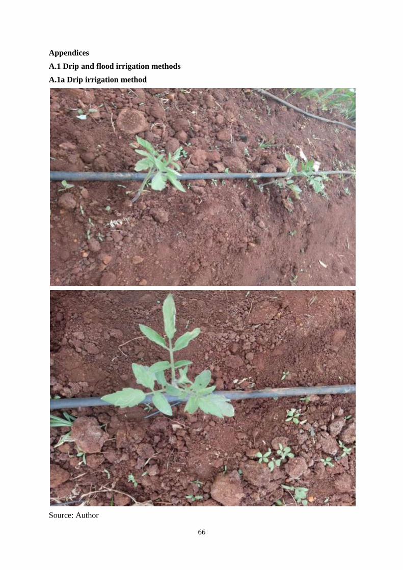
66
Appendices
A.1 Drip and flood irrigation methods
A.1a Drip irrigation method
Source: Author

67
A.1b Flood irrigation method
Source: Author

68
A.2: Questionnaire used for the research data collection
Questionnaire
Information sought for MSc. research in Rural Development by Rashmi.K.S. Faculty of
Bio-Science Engineering, University of Ghent, Belgium.
Title: “DRIP IRRIGATION TECHNOLOGY IN HARD ROCK FARMING AREAS.
TESTING JEVONS PARADOX IN KARNATAKA, INDIA.”
1. Name of the farmer: Date of data collection: - 02-2017
Address:
Mobile No:
Education:
1a. Is major part of your farm income shared from irrigated land – Yes / No
From how many years you are using drip/ flood irrigation………
2. Family details: Type of family: Nuclear / Joint
Household is a group of people who live together and take food from the same pot.
A household member is a person who lives in the household for at least six month and at least
three days in each week of those months.
B1 Household
members
No. 1 2 3 4 5
A. Male adults
(16 and above)
Relation to
respondent
Main
occupation
Education
B Female adults
(16 and above)
Relation to
respondent
Main
occupation
Education
C Girls under 16 Relation to
respondent
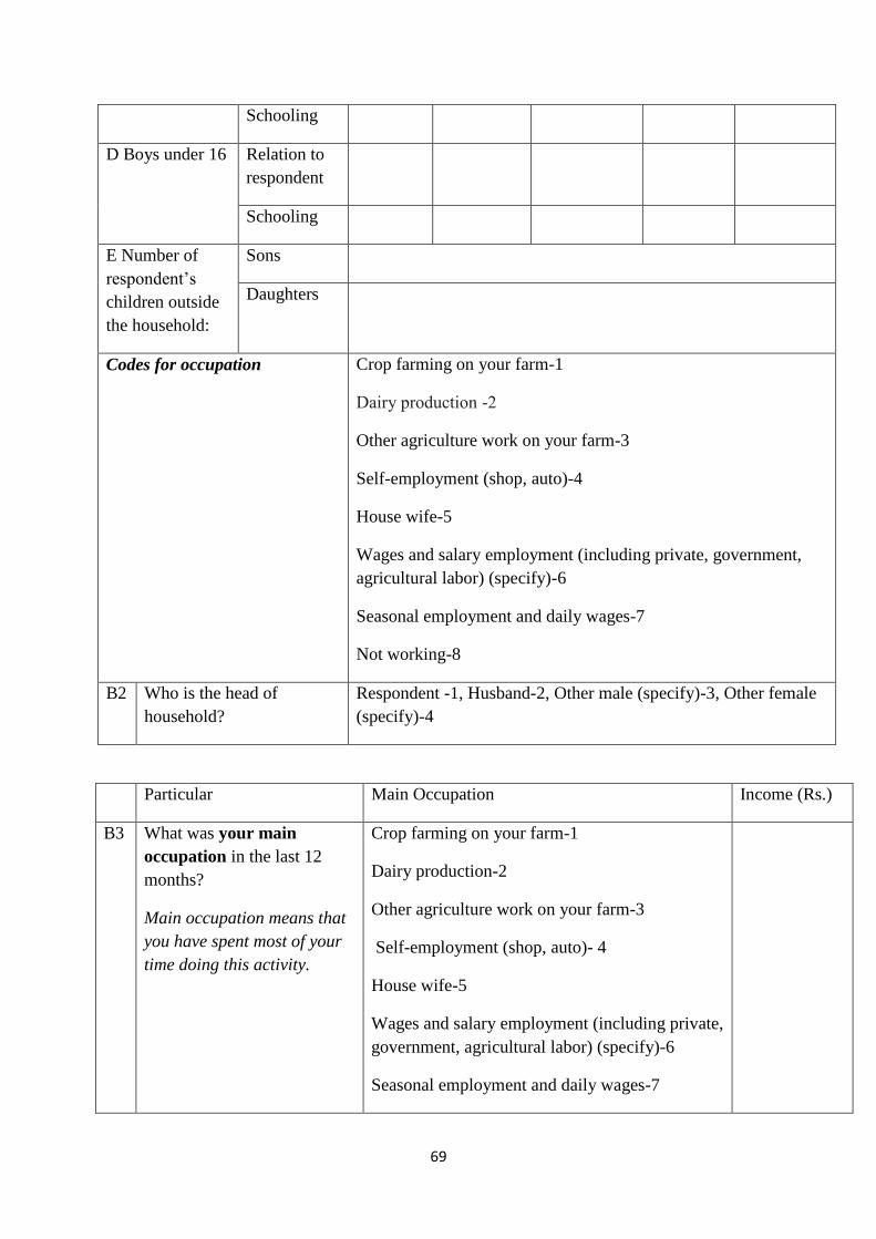
69
Schooling
D Boys under 16 Relation to
respondent
Schooling
E Number of
respondent’s
children outside
the household:
Sons
Daughters
Codes for occupation Crop farming on your farm-1
Dairy production -2
Other agriculture work on your farm-3
Self-employment (shop, auto)-4
House wife-5
Wages and salary employment (including private, government,
agricultural labor) (specify)-6
Seasonal employment and daily wages-7
Not working-8
B2 Who is the head of
household?
Respondent -1, Husband-2, Other male (specify)-3, Other female
(specify)-4
Particular Main Occupation Income (Rs.)
B3 What was your main
occupation in the last 12
months?
Main occupation means that
you have spent most of your
time doing this activity.
Crop farming on your farm-1
Dairy production-2
Other agriculture work on your farm-3
Self-employment (shop, auto)- 4
House wife-5
Wages and salary employment (including private,
government, agricultural labor) (specify)-6
Seasonal employment and daily wages-7

70
Not working-8
What is your subsidiary
occupation
Crop farming on your farm-1
Dairy production-2
Other agriculture work on your farm-3
Self-employment (shop, auto)-4
House wife-5
Wages and salary employment (including private,
government, agricultural labor) (specify)-6
Seasonal employment and daily wages-7
Not working-8
2b. Major crop: plantation/ field crop
If plantation crop, age of the orchard……… year
3. Credit details of the farmers
Credit type Amount (Rs.) Duration
of loan
(years)
Interest
(%)
Credit Institution Distance to
Institution
from Village
(km)
3. ASSET
A. Land Holdings
Sl.
No. Particulars Irrigation land Dry land
Irrigation Source (tank /
well)
1. Owned land (in acres)
2. Leased in land (in acres)
3. Leased out land (in acres)
4. Land value / acre (in rupees)
5. No. of fragments
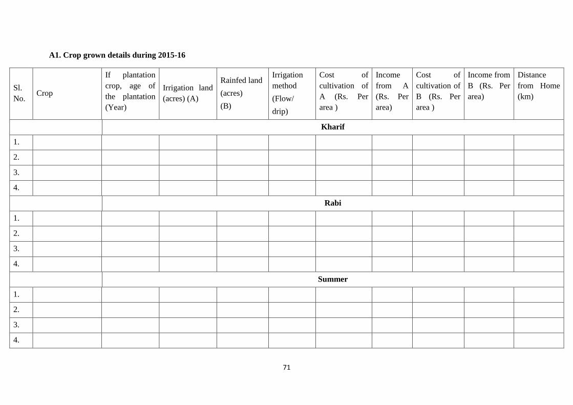
71
A1. Crop grown details during 2015-16
Sl.
No. Crop
If plantation
crop, age of
the plantation
(Year)
Irrigation land
(acres) (A)
Rainfed land
(acres)
(B)
Irrigation
method
(Flow/
drip)
Cost of
cultivation of
A (Rs. Per
area )
Income
from A
(Rs. Per
area)
Cost of
cultivation of
B (Rs. Per
area )
Income from
B (Rs. Per
area)
Distance
from Home
(km)
Kharif
1.
2.
3.
4.
Rabi
1.
2.
3.
4.
Summer
1.
2.
3.
4.

72
A2. Irrigated area details according to 2015-16:
Sl. No. Particulars In acres Income (Rs. Per total
area)
1. Total area cropped per year
2. Drip/flow irrigated area per season
3. Flow irrigated area per season
4. Drip irrigated area per year
5. Flood irrigated area per year
6. irrigated area per year before drip
irrigation
7. irrigated area per season before drip
irrigation
B. Farm Machinery, Implements
Sl. No. Name of the machinery No. Year of
Purchase
Book value
(Rs.)
Annual Income from hiring-
out machinery (Rs.)
1 Tractor (……. hp) with
accessories
2 Power tiller (……. hp)
with accessories
3 Any other machinery /
equipments
4 Bullock Cart
C. Livestock
Sl.
No. Particulars No.
Milk yield
from milch
animals
Income from sale of milk/
poultry/sheep/pigs / hire charges received
from draught animals per year
1 Draught animals
2
Milch animals
a. Local cow
b. Crossbred cow
c. She buffalo

73
3 Calves and Heifers
(below 1 year)
4 Sheep
5 Goats
6 Pigs
7 Poultry
4. Inventory-identification, reasons for functioning / non-functioning of bore wells
on the farm.
4a. Number of bore wells of the farmers
4b. Details about functional bore wells
Bore well
Location
and Identity in
the farm
Interference distance
from neighbour bore
well (m)
Distance from
water source
(pond, tank) (m)
Present Age
of the bore
well (Year)
1.
2.
3.
4.
5.
NOTE: For Identification write in farmers’ own description like ‘Raste Bhavi’; ‘Thotada
Bhavi’; ‘Mane bore’

74
5. Details of functional bore wells owned
Particulars Well No.1
Working /failed
Well No.2
Working /failed
Well No.3
Working /failed
Magnit
ude Investment Magnitude Investment Magnitude Investment
1.Year of drilling/digging
2. Drilling depth (ft)
3a. Diameter of well (inches)
3b. Dimension of dug well *
4. Casing Length (ft)
5. Length of pipes (delivery)
6. Pump HP / stages ex: 5/7
7. Pump placement depth (ft)
8. Pump house
9. Electrical installation cost
10. Other costs (specify)
11. H20 Storage structure (1)*
12. H20 Storage structure (2) *
Yield of the well
13. Year of construction
14. Drip irrigation area in
acres
Crop/s cultivated in drip
Particulars Mag. Invsmt (Rs.) Mag. Invsmt (Rs.) Mag. Invsmt (Rs.)
No. of pipes
Length of drip pipes in feet

75
Drippers at every ___ foot (every
1 or 1.5 feet etc)
No. of drips or holes per pipe
15. No. of emitters /no. of
drippers
No. of liters dripped per hour
(estimate this)
16. Year installed
17. Subsidy received
*Dimension: Length X Breadth X Depth; Groundwater quality: Good / Average / Poor
Is well failure common in the region? Yes / no
If yes, Reasons for well failure in the region:
1. Densely spaced Wells;
2. Initial failure;
3. Water intensive crops – name the crop;
4. Frequent power cuts/load shedding;
5. Decreasing number of rainy days
6. Ill-distributed rainfall;
7. Decreasing quantum of rainfall;
8. Tanks not desilted-poor Groundwater recharge;
10. Use of high HP pumps than needed;
11. Did not drill at the point shown by local diviner
12. Did not drill at the point shown by Geologist
13. Well is located outside command area of Irrigation tank;
14. Irrigation tanks are not regularly filled up;
15. Irrigation well is close to successful public drinking water well;
16. Siltation in bore well;
17. Any other specify

76
6. How wells are financed
Particulars Well no _____ Well no _____ Well no _____
Qty Funds(Rs.) Qty Funds (Rs.) Qty Funds (Rs.)
1. By sale of land
2. Sale of jewels (grams)
3. Sale of livestock (number)
4. From Dairy/ Poultry
5. Sale of trees (number)
6. Sale of Perennials
7. Savings from farm net returns
8. Relatives and friends
9. Borrowing from Banks / Cooperatives
10. Outstanding debt from well/s & IP set/s
7. How drip irrigation is financed
Particulars Land area ….. (acres)
Land area …..
(acres)
Land area …..
(acres)
Qty Funds (Rs.) Qty Funds (Rs.) Qty Funds (Rs.)
1. By government assistance
2. Own Finance
a. Savings
b. Returns from previous crop sale
c. Credit and interest rate
8. Crop wise Costs and returns from crop enterprises on the farm for the year 2015-16
Crop: Field or plantation
Season_____Crop______
Var___ Area______
Season_____Crop______
Var___ Area______
Season_____Crop______
Var___ Area______

77
I. If Flow irrigation
1.Frequency of irrigation
(once in)
2.Hours to irrigate this area
3. Hours of irrigation per time
4. Duration of irrigation (e.g.
Days/weeks/months)
Crop: Field or plantation
Season_____Crop______
Var___ Area______
Season_____Crop______
Var___ Area______
Season_____Crop______
Var ___ Area______
Quantity Value Quantity Value Quantity Value
II. If Drip Irrigation
1.No.of emitters in area
2. Discharge per emitter in
liters per hour
3. No. of hours of drip for
each irrigation
4. Frequency of drip irrigation
(once in)
If sprinkler irrigation add….as
above
5. Duration of irrigation (e.g.
Days/weeks/months)
1. man days of labor
2. woman days of labour
3.Bullock labour days
3.Machine hours
4.Seeds / planting material
5.Manure (cart loads)
6.Fertilizer type (Kg)
a)
b)
c)
7.PPCs: Liquid

78
8. PPCs Dust
9. Transport costs
Packing costs
Marketing costs
10. Main product (Qtl)
11. Price of main product
12. By product (Qtl)
13. Price of By product
9. Agriculture training
Training type Duration of Training
(days)
Place of training Sponsored institute
10. Agriculture Market access
Product sold Market accessing Distance from your
village (km)
Commission per….
79
A.3: Data collection photos
Photo 1
Source: Author
Photo 2
Source: Author
80
Photo 3
Source: Author
Photo 4
Source: Author

81
A.4: Correlation of Instrumental variables with loan amount borrowed by the famer
from bank/s
Particular
Loan amount
borrowed by farmer
from bank
Total distance to loan
institution from
farmer’s village
Total distance to
product market from
farmers village
Loan amount
borrowed by farmer
from bank
1.00 0.56 0.43
Total distance to loan
institution from
farmer’s village
0.56 1.00 0.03
Total distance to
product market from
farmer’s village
0.43 0.03 1.00
Source: Author