Embed Size (px)
Citation preview

drda: An R package for dose-response data analysis
Alina Malyutina
University of HelsinkiJing Tang
University of HelsinkiAlberto Pessia
University of Helsinki
Abstract
Analysis of dose-response data is an important step in many scientiĄc disciplines,including but not limited to pharmacology, toxicology, and epidemiology. The R packagedrda is designed to facilitate the analysis of dose-response data by implementing efficientand accurate functions with a familiar interface. With drda, it is possible to Ąt models bythe method of least squares, perform goodness of Ąt tests, and conduct model selection.Compared to other similar packages, drda provides, in general, more accurate estimates inthe least-squares sense. This result is achieved by a smart choice of the starting point in theoptimization algorithm and by implementing the Newton method with a trust region withanalytical gradients and Hessian matrices. In this article, drda is presented through thedescription of its methodological components and examples of its user-friendly functions.Performance is Ąnally evaluated using a real, large-scale drug sensitivity screening dataset.
Keywords: curve Ątting, dose-response, drug sensitivity, logistic function, nonlinear regression.
1. Introduction
Inferring dose-response relationships is indispensable in many scientiĄc disciplines. In cancerresearch, for example, estimating the magnitude of a chemical compound effect on cancer cellsholds substantial promise for clinical applications. The dose-response relationship is oftenmodeled via a nonlinear parametric function expressed as a dose-response curve. The Ąttingof a curve to dose-response measurements is often achieved by choosing the parameter valuesthat minimize the difference between the curve and the observations. Since conclusions aboutefficacy are based on the estimated dose-response curve, it is therefore of great importance todetermine the curve parameters as accurately as possible.
Currently, there are multiple R packages that provide tools for the dose-response Ątting,such as drc (Ritz, Baty, and Gerhard 2015), nplr (Commo and Bot 2016), and DoseFinding
(Bornkamp, Pinheiro, and Bretz 2019). The drc package contains various functions for non-linear regression analysis of biological assays. It allows the user to choose a nonlinear modelfor the dose-response curve Ątting from a wide spectrum of sigmoid functions, which are nor-mally used to capture the dose-response relationship as their S-shape is in line with empiricalobservations from experiments. The most common model is the 4-parameter generalizedlogistic function.
In the drc package, a user can specify initial model parameters to facilitate the optimizationprocess or rely on the default starter functions. The package also enables a user to set theweights for the observations to adjust the possible variance heterogeneity in the responsevalues. The parameter estimation procedure is achieved by the least squares method, using
2 drda: dose-response data analysis
a maximum likelihood approach with the default assumption of normality for inferentialpurposes.
In contrast to drc, the nplr package focuses only on generalized logistic models and does notallow to select the data distribution. As a new feature, the package facilitates the choiceof observation weights via implementing three options: residual-based, standard (or within-replicate variance-based), and general, which utilizes the Ątted response values. Additionally,the package provides conĄdence intervals on the predicted doses and the trapezoid and theSimpsonŠs rule (Abramowitz and Stegun 1965, Chapter 25) to evaluate the area under thecurve.
The DoseFinding package provides more Ćexibility than drc and nplr. It allows for the Ąttingof multiple linear and nonlinear dose-response models and to design dose-Ąnding experiments.Similarly to drc, it provides several options for the data distribution, but as default it usesassumption of normality with equal variance. Compared to drc and nplr, the DoseFinding
package utilizes a grid search as a starting point selection method in case the user did notspecify its own. It also applies boundaries to parameters of a nonlinear model either speciĄedby a user or through internal default settings.
To Ąnd the optimal parameter in a high-dimensional space, all packages apply iterative New-ton methods, which are widely used numerical procedures for Ąnding the minimum of adifferentiable function (Nocedal and Wright 2006). The drc package directly calls the R
optim() function that implements the Broyden-Fletcher-Goldfarb-Shanno (BFGS) method(Fletcher 2000) for unconstrained optimization, or limited-memory BFGS (L-BFGS-B), whichhandles simple box constraints for constrained optimization (Liu and Nocedal 1989). Thesetwo methods represent quasi-Newton methods, which are frequently used in cases when thefunction derivatives are not feasible or too complicated to obtain, as they utilize numericalapproximations of the functionŠs Hessian matrix. In contrast, the nplr package relies on thenlm() function, which uses the classic Newton approach. By default, both the gradient andHessian are approximated numerically, however the user can provide themselves the Ąrst andsecond analytical derivatives. The DoseFinding package applies different optimization rou-tines depending on the models of choice. For sigmoid and logistic models, which have twolinear and two nonlinear function parameters, the package performs numerical optimizationjust for nonlinear ones, while optimizing the linear parameters in every iteration of the al-gorithm. At its core, DoseFinding applies the R nlminb() function, using a quasi-Newtonalgorithm similar to the BFGS method utilized by drc.
While all packages have been extremely helpful with a wide range of real applications, wefound that they often present inconsistent results when applied to the same data with thesame logistic model. We introduce here the R package drda, which provides a novel and moreaccurate dose-response data analysis using logistic curves via: (i) applying a more advancedNewton method with a trust region; (ii) relying on analytical gradient and Hessian formulasinstead of numerical approximations; (iii) establishing a smart initialization procedure toincrease the chances of converging to the global solution; (iv) providing tools to compare theĄtted curve against a linear model or other logistic models; (v) computing conĄdence intervalsfor the estimated parameters and for the whole dose-response curve; (vi) implementing plotfunctionality to compare multiple models in a user-friendly way.
The most important feature of any optimization routine remains the closeness of its solutionto the true least square estimates. In case of biological assays, it depends on the ability of

Alina Malyutina, Jing Tang, Alberto Pessia 3
the Ątted curve to describe the dose-response data correctly. One of the main disadvantageswhen it comes to numerical optimization is the possibility of converging to a local optimuminstead of the correct answer we seek. This situation can easily happen when either thefunction is not well approximated by a quadratic shape in a neighborhood of the currentcandidate solution, or when the starting point is far from the global optimum (either thealgorithm is not able to converge in a reasonable number of steps or it simply converges to awrong solution). To cope with such scenarios, we implement here the Newton method with atrust region (Steihaug 1983), which has been shown to be a robust optimization technique formitigating issues usually encountered in unconstrained optimization problems. The methodis more stable than other Newton-based methods, especially for cases when it is problematicto approximate a function with a quadratic curve (Sorensen 1982). Additionally, drda usesa two-step initialization algorithm in order to ensure the right direction in the optimizationroutine. With our strategy, drda is able to Ąnd the true least squares estimate in problematiccases where the drc, nplr, and DoseFinding packages instead fail.
Once the least squares estimate is found, drda provides the user with routines for assessinggoodness of Ąt and reliability of the estimates. Assuming a Gaussian distribution with equalvariance for the observed data, it is possible to compare the Ątted model against, for example,a Ćat horizontal line or a logistic model with a different number of parameters. The drda
package provides the likelihood ratio test (LRT), the Akaike information criterion (AIC)(Akaike 1974), and the Bayesian information criterion (BIC) (Schwarz 1978) as a way tocompare the goodness of Ąt of competing models.
The paper is organized as follows: We Ąrst describe the methodological components of drda
in Section 2; show how the package is implemented in Section 3; include practical examples inSection 3.2; and provide a comparison of drda against packages DoseFinding, drc, and nplr
using a high-throughput dose-response dataset in Section 4. We conclude the article with asummary and discussion in Section 5.
2. Methodological framework
2.1. Generalized logistic function
Package drda implements the generalized logistic function as the core model for Ątting dose-response data. The generalized logistic function, also known as RichardsŠ curve (Richards1959), is the 5-parameter function
f(x;ψ) = α+ (β − α) (1 + ν exp¶−η(x− ϕ)♢)−1/ν (1)
solution to the differential equation
∂
∂xf(x;ψ) =
η
ν
1 −
f(x;ψ) − α
β − α
ν
(f(x;ψ) − α)
where ψ = (α, β, η, ϕ, ν)T .
Throughout this article, and in our package, we will use the convention β > α to avoididentiĄability issues. For example, when β < α, it is always possible to modify the remainingthree parameters to obtain an equivalent function. To have a sigmoidal curve, a common
4 drda: dose-response data analysis
requirement in dose-response data analysis, we will also assume that ν ≥ 0. When ν < 0, infact, the curve is unbounded or even complex.
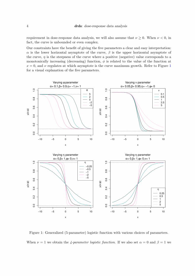
Our constraints have the beneĄt of giving the Ąve parameters a clear and easy interpretation:α is the lower horizontal asymptote of the curve, β is the upper horizontal asymptote ofthe curve, η is the steepness of the curve where a positive (negative) value corresponds to amonotonically increasing (decreasing) function, ϕ is related to the value of the function atx = 0, and ν regulates at which asymptote is the curve maximum growth. Refer to Figure 1for a visual explanation of the Ąve parameters.
−10 −5 0 5 10
0.0
0.2
0.4
0.6
0.8
1.0
Varying φ parameter
x
µ(x;ψ
)
α= 0.1,β= 0.9,η= −1,ν= 1
φ
520−2−5
−10 −5 0 5 10
0.0
0.2
0.4
0.6
0.8
1.0
Varying ν parameter
x
µ(x;ψ
)
α= 0.05,β= 0.95,η= −1,φ= 0
ν0.10.512.55
−10 −5 0 5 10
0.0
0.2
0.4
0.6
0.8
1.0
Varying η parameter
x
µ(x;ψ
)
α= 0,β= 1,φ= 0,ν= 1
η
−0.25−0.5−1−2−5
−10 −5 0 5 10
0.0
0.2
0.4
0.6
0.8
1.0
Varying η parameter
x
µ(x;ψ
)
α= 0,β= 1,φ= 0,ν= 1
η
0.250.5125
Figure 1: Generalized (5-parameter) logistic function with various choices of parameters.
When ν = 1 we obtain the 4-parameter logistic function. If we also set α = 0 and β = 1 we
Alina Malyutina, Jing Tang, Alberto Pessia 5
obtain the 2-parameter logistic function. When ν = 1 the parameter ϕ represents the valueat which the function is equal to its midpoint, that is (α+β)/2. In such a case, as a measureof drug potency, ϕ is also known as the half maximal effective log-concentration or log-EC50.As a a measure of antagonist drug potency, ϕ is also known as the half maximal inhibitory
log-concentration (log-IC50). When ν → 0 we obtain the Gompertz function, i.e.
limν→0
f(x;ψ) = α+ (β − α) exp ¶− exp¶−η(x− ϕ)♢♢
The Emax model (Macdougall 2006), often found in dose-response studies, is formally equiv-alent to the 4-parameter logistic function. The difference between the two models is simplythe parametrization of the scale used for the variable x. If the Emax model is deĄned as
y(D;λ) = E0 + EmaxDN
DN + EDN50
then the equivalent 4-parameter logistic function (ν = 1) is obtained by the transformationsD = ex, E0 = α, Emax = β − α, N = η, ED50 = eϕ.
2.2. Normal nonlinear regression
For a particular dose dk (k = 1, . . . ,m) let (yki, wki)T represent respectively the i-th observed
outcome and its associated positive weight. If observations have all the same importance, wesimply set wki = 1 for all k and i. We assume that each unit has expected value and variance
E[Yki♣dk,ψ] = µ(dk;ψ)
V[Yki♣wki, σ] =σ2
wki
where µ(dk;ψ) is a nonlinear function of the dose dk and a vector of unknown parametersψ. Parameter σ > 0 is instead the standard deviation common to all observations. Inour package, µ(dk;ψ) is simply the generalized logistic function (1) with the transformationx = log(dk).
By assuming the observations to be stochastically independent and Normally distributed, thejoint log-likelihood function is
l(ψ, σ) = −1
2
n log(2π) + n log(σ2) −m∑
k=1
nk∑
i=1
log(wki) +1
σ2
m∑
k=1
nk∑
i=1
wki(yki − yk)2+
+1
σ2
m∑
k=1
wk.(yk − µ(dk;ψ))2
where nk is the sample size at dose k, n =∑
k nk is the total sample size, yk = (∑
iwkiyki)/wk.is the weighted average corresponding to dose dk and wk. =
∑
iwki. Maximum likelihoodestimate ψ is obtained by minimizing the residual sum of squares from the means, i.e.
ψ = arg minψ∈Ψ
1
2
m∑
k=1
wk.(yk − µ(dk;ψ))2 = arg minψ∈Ψ
g(ψ) (2)

6 drda: dose-response data analysis
Maximum likelihood estimate of the variance is
σ2 =1
n
m∑
k=1
nk∑
i=1
wki(yki − µ(dk; ψ))2 =D2
n
while its unbiased estimate is
s2 =D2
n− p
where p is the total number of parameters estimated from the data.
For convenience from now on we will use the simpliĄed notation µk to denote the functionµ(dk;ψ). It is important to remember that µk will always be a function of a dose dk and aparticular parameter value ψ. We will also use the notation g(s) and g(st) to denote respec-tively the Ąrst- and second-order partial derivatives of function g(ψ), with respect Ąrst to ψsand then ψt.
Partial derivatives of the sum of squares g(ψ) are
g(s) =m∑
k=1
wk.(µk − yk)µ(s)k
g(st) =m∑
k=1
wk.
(µk − yk)µ(st)k + µ
(s)k µ
(t)k
The gradient and Hessian of g(ψ) are therefore
∇ψg =m∑
k=1
wk.(µk − yk)∇ψµk
Hψg =m∑
k=1
wk.
(µk − yk)Hψµk + (∇ψµk) (∇ψµk)T
From the previous expressions we can easily retrieve the observed Fisher information matrix,which is the negative Hessian matrix of the log-likelihood evaluated at the maximum likelihoodestimate, as
I(ψ, σ) =1
σ2
Hψg −2∇ψg/σ
−2 (∇ψg)T /σ q
(3)
where
q =3∑
k
∑
iwki(yki − µk)2
σ2− n
It is also worth noting that the (expected) Fisher information matrix is
I(ψ, σ) =1
σ2
∑
k wk. (∇ψµk) (∇ψµk)T
0
0 3∑
k
∑
iwki − n
(4)
2.3. Optimization by Newton method with a trust region
Closed-form formula of the maximum likelihood estimate ψ, that is the solution of equation(2), is in general not available for nonlinear regression models. We can, however, try tominimize numerically the sum of squares g(ψ).

Alina Malyutina, Jing Tang, Alberto Pessia 7
Suppose that our algorithm is at iteration t with current solution ψt. We want to Ąnd a newstep u such that g(ψt + u) < g(ψt). We start by illustrating the standard Newton method.We approximate our function by a second-order Taylor expansion, that is
g(ψt + u) ≈ g(ψt) + ∇Tψtu+
1
2uTHψt
u
The theoretical minimum is obviously attained when the gradient with respect to u is zero,that is ∇ψt
+ Hψtu = 0 or u = −H
−1ψt
∇ψt. The NewtonŠs candidate solution for iteration
t+ 1 is often presented asψt+1 = ψt − γH
−1ψt
∇ψt
where 0 < γ ≤ 1 is a modiĄer of the step size for ensuring convergence (Armijo 1966).
When the method converges the algorithm is quadratically fast, or at least superlinear (Bon-nans, Gilbert, Lemarechal, and Sagastizábal 2006): the closer g(ψ) is to a quadratic functionthe better its Taylor approximation, the better the algorithm convergence properties.
−6 −4 −2 0 2
0.0
0.2
0.4
0.6
0.8
1.0
1.2
log(dose)
Perc
ent via
bili
ty
True estimate
BFGS
A)
η
φ
0.2
0.4
0.6 0.8
1
1
1.5
3 3.4
−2.0 −1.5 −1.0 −0.5 0.0
−20
−10
010
20
B)
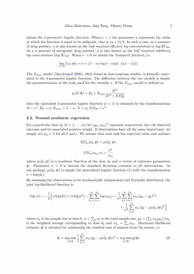
Figure 2: Problematic real data (cell line: BT-20, compound: BI-2536, dataset: CTRPv2)(Rees et al. 2016; Seashore-Ludlow et al. 2015; Basu et al. 2013)). A) 4-parameter logisticfunction as Ątted by the BFGS algorithm. Starting point ψ = (α, β, η, ϕ)T = (0, 1,−1, 0)T .B) Contour plot of the residual sum of squares g(ψ) with respect to parameters η and ϕ.Fixed parameters α = 0 and β = 1.
When the Hessian matrix is almost singular it is still possible to apply quasi-Newton methods(Luenberger and Ye 2008) to (try) avoid convergence problems. In our nonlinear regressionsetting, however, we might have the extra complication of an objective function far from aquadratic shape, so that the (quasi-)Newton method might fail to converge. Although this

8 drda: dose-response data analysis
situations can be thought to be rare, they are often encountered in real applications. Forexample, in Figure 2 we show a problematic surface that the quasi-Newton BFGS algorithm,as implemented by the base R function optim(), is not able to properly explore.
We will try to overcome the issues in the optimization by focusing our search only in aneighborhood of the current estimate, that is using a trust-region around the current solutionψt. The problem to solve is now
minu∈Rp
g(ψt) + ∇Tψtu+
1
2uTHψt
u s.t. ♣♣u♣♣ ≤ ∆t
where ∆t > 0 is the trust-region radius. Our implementation is based on the exposition ofNocedal and Wright (2006) and follows closely that of Mogensen and Riseth (2018). BrieĆy,at each iteration we compute the standard NewtonŠs step and accept the new solution ifit is within the trust-region. If the NewtonŠs step is outside the admissible region we tryan alternative step by a linear combination of the NewtonŠs step and the steepest descentstep, with the constraint that its length is exactly equal to the radius ∆t (dogleg method).This new alternative step is then accepted or rejected on the basis of the actual reduction inthe function value. The region radius ∆t+1 for iteration t + 1 is adjusted according to thelength and acceptance of the step just computed. For more details, we refer the reader to theextensive discussion found in Nocedal and Wright (2006).
2.4. Algorithm initialization
One of the major challenges in Ątting nonlinear regression models is choosing a good startingpoint for initializing the optimization algorithm. Looking at the example in Figure 2, thechoice of ψ0 = (0, 1,−1, 0)T made the BFGS algorithm converge to a local optimum while aglobal optimum might have been found if a better starting point was chosen.
First of all, we present the closed-form maximum likelihood estimates α and β when all otherparameters have been Ąxed. DeĄne hk = (1 + ν exp(−η(xk − ϕ)))−1/ν , where xk = log(dk),and assume it to be known. Our mean function is now
µk(α, β) = α+ (β − α)hk = (1 − hk)α+ hkβ
while the residual sum of squares becomes
g(α, β) =1
2
m∑
k=1
wk.(yk − (1 − hk)α− hkβ)2
with gradient
g(α) = −m∑
k=1
(1 − hk)wk.yk + αm∑
k=1
(1 − hk)2wk. + β
m∑
k=1
hk(1 − hk)wk.
g(β) = −m∑
k=1
hkwk.yk + αm∑
k=1
hk(1 − hk)wk. + βm∑
k=1
h2kwk.
It is easy to prove that the gradient is equal to zero for
α =
(∑
k h2kwk.
)
(∑
k(1 − hk)wk.yk) − (∑
k hk(1 − hk)wk.) (∑
k hkwk.yk)
(∑
k hk(1 − hk)wk.)2 − (
∑
k(1 − hk)2wk.)(∑
k h2kwk.
)
β =
(∑
k(1 − hk)2wk.
)
(∑
k hkwk.yk) − (∑
k hk(1 − hk)wk.) (∑
k(1 − hk)wk.yk)
(∑
k hk(1 − hk)wk.)2 − (
∑
k(1 − hk)2wk.)(∑
k h2kwk.
)
(5)
Alina Malyutina, Jing Tang, Alberto Pessia 9
Our initialization strategy is made of two steps. The Ąrst step is done by setting ν0 = 1and obtaining an initial guess for η0 and ϕ0, for example by choosing them at random or byevaluating the objective function on a small grid of values. We then evaluate the maximumlikelihood estimates (5) and set α0 = α and β0 = β. The second step is running the standardNewton method starting from ψ0. The solution just found is then passed to our trust regionimplementation for further reĄning.
When the likelihood function is well-behaved, the standard Newton method in the secondstep is very fast and efficient, and most of the times will converge to the global optimum.However, when the function is problematic, we sacriĄce speed for accuracy by supplying ourtrust region method with the local optimum found so far.
2.5. Statistical inference
When closed-form solutions of maximum likelihood estimates are missing, also closed-formexpressions of other inferential quantities are not available. Fortunately, we can still rely onasymptotic, large sample size considerations, to obtain approximate values of quantities ofinterest. Obviously, the larger the sample size the better the approximation.
Using either versions (3) or (4) of the Fisher information matrix we can calculate approximateconĄdence intervals. In fact, we can think of the Fisher information matrix as an approximateprecision matrix, so that we only have to invert the matrix and take diagonal elements asapproximate variance estimates. In our package we use the observed Fisher informationmatrix (3) because it is shown to perform better with Ąnite sample sizes (Efron and Hinkley1978). As an example, an approximate conĄdence interval for generic parameter ψj is
ψj ± tn−p,α
√
I(ψ, σ)−1
jj
where tn−p,α is the appropriate quantile of level α of a StudentŠs t-distribution with n −
p degrees of freedom and
I(ψ, σ)−1
jjis the j-th element in the diagonal of the inverse
observed Fisher information matrix. Using the Delta method we can compute approximatepoint-wise conĄdence intervals for the mean function
µ(dk; ψ) ± tn−p,α
√
s2
∇ψµkT
Hψf
−1
∇ψµk
or for a new, yet to be observed, value y(d)
µ(d; ψ) ± tn−p,α
√
s2
1 +
∇ψµT
Hψf
−1
∇ψµ
We can also construct a (conservative and approximate) conĄdence band over the whole meanfunction µ(·;ψ) with the correction proposed by Gsteiger, Bretz, and Liu (2011)
µ(d; ψ) ±
√
qp,αs2
∇ψµT
Hψf
−1
∇ψµ
where qp,α is the appropriate quantile of level α of a χ2-distribution with p degrees of freedom.
3. Using drda

10 drda: dose-response data analysis
3.1. General overview
The main function of drda is drda() with signature
drda(
formula, data, subset, weights, na.action, mean_function = "logistic4",
is_log = TRUE, lower_bound = NULL, upper_bound = NULL, start = NULL,
max_iter = 500
)
The Ąrst argument, formula, is a symbolic representation in the form y ~ x of the model tobe Ątted, where y is the vector of responses and x is the vector of log-doses.
data is an optional argument, typically a data.frame object, containing the variables in themodel. When data is not speciĄed, the variables are taken from the environment where thefunction is being called.
subset is a logical vector, or a vector of indices, specifying the portion of data to be used formodel Ątting.
weights is an optional argument that speciĄes the weights to be used for Ątting. Usuallyweights are used in situations where observations are not equally informative, i.e. when it isknown that some of the observations should have a smaller or larger impact on the Ąttingprocess. If the weights argument is not provided then the ordinary least squares method isapplied.
na.action deĄnes a function for handling NAs found in data. The default option is to usena.omit(), i.e. to remove all data points associated with the missing values.
mean_function argument speciĄes the model that should be estimated. In the current ver-sion of the package the argument can be any of Ślogistic5Š, Ślogistic4Š, Ślogistic2Š, orŚgompertzŠ. Each model is explained in detail in Section 2.1. By default, the 4-parameterlogistic function is chosen.
is_log is a logical indicator specifying if the x variable in the formula argument is alreadyon the log scale. The default value is TRUE, thus, if x is given on a natural scale, is_log
argument should be set to FALSE.
Arguments lower_bound and upper_bound are used for performing constrained optimiza-tion. They serve as the minimum and maximum values allowed for the model parameters.They are vectors of length equal to the number of parameters of the model speciĄed bythe mean_function argument. Values -Inf and Inf are allowed. The parameters for the5-parameter generalized logistic function are listed in the following order: α, β, η, ϕ, ν. Forthe other models the order is preserved but some of the parameters are excluded. Obvi-ously, values in upper_bound must be greater than or equal to the corresponding values inlower_bound.
start represents a vector of starting values for the parameters.
Finally, the max_iter argument sets the value for the maximum number of iterations in theoptimization algorithm.
After the call to drda(), all the common functions expected for a model Ąt are available:coef(), deviance(), logLik(), plot(), predict(), residuals(), sigma(), summary(),weights().
Alina Malyutina, Jing Tang, Alberto Pessia 11
To evaluate the efficacy of the treatment it is also possible to compute the normalized areaunder or above the curve. The functions are respectively
nauc(drda_object, xlim = c(-10, 10), ylim = c(0, 1))
naac(drda_object, xlim = c(-10, 10), ylim = c(0, 1))
The two-element vector xlim deĄnes the interval of integration, on the log-scale, with respectto x. The two-element vector ylim deĄnes the theoretical minimum and maximum valuesfor the response variable y. Therefore, xlim and ylim together deĄne a rectangle that ispartitioned into two regions by the dose-response curve. The normalized area under thecurve (NAUC) is deĄned as the area of the ŞlowerŤ rectangle region divided by the total areaof the rectangle. The normalized area above the curve (NAAC) is simply its complement, i.e.1 - NAUC.
When xlim and ylim are not explicitly chosen, the default values are set respectively toc(-10, 10) and c(0, 1). The xlim default value was chosen on the basis of dose rangesthat are commonly found in the literature, and made symmetric around zero so that NAUCand NAAC values are equal to 0.5 in the standard logistic model. In the majority of realapplications the response variable y is usually a relative measure against a control treatment,therefore the default value for ylim is chosen to be c(0, 1).
3.2. Usage examples
First of all, we load the package.
R> library(drda)
We then deĄne an example dataset to demonstrate how to use drda.
R> dose <- rep(c(0.0001, 0.001, 0.01, 0.1, 1, 10, 100), each = 3)
R> relative_viability <- c(
+ 0.877362, 0.812841, 0.883113, 0.873494, 0.845769, 0.999422, 0.888961,
+ 0.735539, 0.842040, 0.518041, 0.519261, 0.501252, 0.253209, 0.083937,
+ 0.000719, 0.049249, 0.070804, 0.091425, 0.041096, 0.000012, 0.092564
+ )
This example imitates an experiment where seven drug doses have been tested three timeseach. Relative viability measures have been obtained for each dose-replicate pair and, in thiscase, comprise 21 values in the (0, 1) interval. Note that any Ąnite real number is acceptedas a possible valid outcome.
Default fitting
The drda() function can be applied directly to the two variables via setting is_log to FALSE.
R> fit <- drda(relative_viability ~ dose, is_log = FALSE)
We can obtain exactly the same Ątting using the log-doses and ignoring the is_log argumentand storing the variables into a data frame.

12 drda: dose-response data analysis
R> log_dose <- log(dose)
R> test_data <- data.frame(d = dose, x = log_dose, y = relative_viability)
R> # the following calls are equivalent
R> fit <- drda(relative_viability ~ log_dose)
R> fit <- drda(y ~ d, data = test_data, is_log = FALSE)
R> fit <- drda(y ~ x, data = test_data)
To obtain summaries the user can apply the summary() function to the fit object.
R> summary(fit)
Call: drda(formula = y ~ x, data = test_data)
Pearson Residuals:
Min 1Q Median 3Q Max
-1.81632 -0.45751 -0.02341 0.20617 2.04357
Parameters:
Estimate Lower .95 Upper .95
Minimum 0.05207 -0.001967 0.106
Maximum 0.87914 0.828166 0.930
Growth rate -1.14335 -1.683129 -0.604
Midpoint at -2.11770 -2.476042 -1.759
Residual std err. 0.06541 0.042006 0.089
Residual standard error on 17 degrees of freedom
Log-likelihood: 29.688
AIC: -51.377
BIC: -47.199
Optimization algorithm converged in 20 iterations
The summary() function provides information about the Pearson residuals, parametersŠ andresidual standard error estimates, and their 95% conĄdence intervals. Together with the actualpoint estimate, the widths of conĄdence intervals are a good starting point for assessing thereliability of the model Ąt. The values of the log-likelihood function, AIC, and BIC are alsoprovided. Finally, the summary() function warns the user if the algorithm converges and ifso, in how many iterations.
Parameter estimates can be accessed using the coef() and sigma() functions, or by accessingthem directly.
R> coef(fit)
alpha beta eta phi
0.0520711 0.8791421 -1.1433476 -2.1177022

Alina Malyutina, Jing Tang, Alberto Pessia 13
R> fit$coefficients
alpha beta eta phi
0.0520711 0.8791421 -1.1433476 -2.1177022
R> sigma(fit)
[1] 0.06541385
R> fit$sigma
[1] 0.06541385
Since the model being Ątted is (1), it is important to note that the the coef() function alwaysreturns the parameter ϕ, in this case the log-EC50, regardless of the scale in which x waspassed to the function. The summary() function, however, will always print the estimate onthe same scale as the original x variable.
Our fit object can be further explored with all the familiar functions expected for a modelĄt:
R> deviance(fit)
[1] 0.07274253
R> residuals(fit)
1 2 3 4 5
-0.001531458 -0.066052458 0.004219542 -0.002202763 -0.029927763
6 7 8 9 10
0.123725237 0.055299691 -0.098122309 0.008378691 0.008888741
11 12 13 14 15
0.010108741 -0.007900259 0.133677782 -0.035594218 -0.118812218
16 17 18 19 20
-0.008068816 0.013486184 0.034107184 -0.011354510 -0.052438510
21
0.040113490
R> logLik(fit)
[1] 29.68848
R> predict(fit)

14 drda: dose-response data analysis
1 2 3 4 5 6
0.87889346 0.87889346 0.87889346 0.87569676 0.87569676 0.87569676
7 8 9 10 11 12
0.83366131 0.83366131 0.83366131 0.50915226 0.50915226 0.50915226
13 14 15 16 17 18
0.11953122 0.11953122 0.11953122 0.05731782 0.05731782 0.05731782
19 20 21
0.05245051 0.05245051 0.05245051
R> predict(fit, x = log(c(0.002, 0.2, 2)))
[1] 0.87156973 0.34872020 0.08403782
Model comparison and selection
The anova() function can be used to compare competing models within the same logisticfamily of models. The constant model, i.e. a Ćat horizontal line, is always included by defaultin the comparisons. When the model being Ątted is not the 5-parameter logistic function, thelatter is always included as the general reference model in the likelihood-ratio test.
R> fit_logi2 <- drda(y ~ x, data = test_data, mean_function = "logistic2")
R> anova(fit_logi2)
Analysis of Deviance Table
Model: 2-parameter logistic
Resid. Df Resid. Dev Df AIC BIC LRT
Constant model 20 2.87131 1 19.811 20.855 77.242
Estimated model 19 0.14354 2 -41.103 -39.014 14.328
Full model (logistic5) 16 0.07255 5 -49.431 -44.209
p-value
Constant model 0.0000000
Estimated model 0.0024909
Full model (logistic5)
Note that the p-value refers here to the likelihood-ratio test with a χ2-distribution asymptoticapproximation. In this particular case we are testing the null hypothesis that our 2-parameterlogistic function is equivalent, likelihood-wise, to the complete 5-parameter logistic function.The signiĄcant result indicates that the 2-parameter logistic function provides a worse Ąt forthe observed data compared to a 5-parameter logistic function.
R> fit_logi4 <- drda(y ~ x, data = test_data, mean_function = "logistic4")
R> fit_gompe <- drda(y ~ x, data = test_data, mean_function = "gompertz")
R> anova(fit_logi2, fit_logi4, fit_gompe)

Alina Malyutina, Jing Tang, Alberto Pessia 15
Analysis of Deviance Table
Model 1: Constant
Model 2: logistic2
Model 3: gompertz
Model 4: logistic4
Model 5: logistic5 (Full)
Model 4 is the best model according to the Akaike Information Criterion.
Resid. Df Resid. Dev Df AIC BIC LRT p-value
Model 1 20 2.87131 1 19.811 20.855 77.242 0.00000
Model 2 19 0.14354 2 -41.103 -39.014 14.328 0.00077
Model 3 17 0.07595 4 -50.472 -46.294 0.959 0.00000
Model 4 17 0.07274 4 -51.377 -47.199 0.054 0.81569
Model 5 16 0.07255 5 -49.431 -44.209
These results indicate the 4-parameter logistic function as the best Ąt for the data. Not onlythe model has the lowest AIC value, but the LRT is also not signiĄcant. Indeed, the data wasgenerated from a 4-parameter logistic function with ψ = (0.02, 0.86,−1,−2) and σ = 0.05.
Weighted fitting
In case when not all of the observations should be utilized equally in the model, the weightsargument can be provided to the drda() function. All the generic functions described aboveare also applicable to a weighted Ąt object.
R> weights <- c(
+ 0.990868, 1.095238, 0.974544, 0.973318, 1.107001, 1.012844, 1.052806,
+ 1.019427, 1.032544, 0.919827, 0.971385, 0.959019, 1.037789, 1.006835,
+ 0.969383, 0.935633, 1.016597, 1.011085, 0.982307, 1.066032, 0.959870
+ )
R> fit_weights <- drda(y ~ x, data = test_data, weights = weights)
R> summary(fit_weights)
Call: drda(formula = y ~ x, data = test_data, weights = weights)
Pearson Residuals:
Min 1Q Median 3Q Max
-1.79403 -0.46630 -0.01527 0.20625 2.03837
Parameters:
Estimate Lower .95 Upper .95
Minimum 0.05176 -0.00314 0.107
Maximum 0.87864 0.82776 0.930
Growth rate -1.13251 -1.66213 -0.603

16 drda: dose-response data analysis
Midpoint at -2.11178 -2.48430 -1.739
Residual std err. 0.06604 0.04241 0.090
Residual standard error on 17 degrees of freedom
Log-likelihood: 29.522
AIC: -51.045
BIC: -46.867
Optimization algorithm converged in 129 iterations
R> weights(fit_weights)
[1] 0.990868 1.095238 0.974544 0.973318 1.107001 1.012844 1.052806
[8] 1.019427 1.032544 0.919827 0.971385 0.959019 1.037789 1.006835
[15] 0.969383 0.935633 1.016597 1.011085 0.982307 1.066032 0.959870
R> residuals(fit_weights, type = "weighted")
1 2 3 4 5
-0.001008649 -0.068584002 0.004677024 -0.001524068 -0.030795978
6 7 8 9 10
0.125179424 0.058144516 -0.097689734 0.009903896 0.008004185
11 12 13 14 15
0.009427869 -0.008268459 0.134622275 -0.037250106 -0.118484884
16 17 18 19 20
-0.007781909 0.013621515 0.034319514 -0.010972588 -0.053849388
21
0.039578170
Constrained optimization
The drda() function allows the choice of admissible values for the parameters by setting thelower_bound and upper_bound arguments appropriately. Unconstrained parameters are setto -Inf and Inf respectively. While setting the constraints manually, one should be careful inchoosing the values as the optimization problem might become very difficult to solve withina reasonable number of iterations.
In the next example the lower bound and upper bound parameters are Ąxed to 0 and 1respectively, the growth rate is allowed to vary in [−5, 5], while the midpoint parameter isleft unconstrained.
R> lb <- c(0, 1, -5, -Inf)
R> ub <- c(0, 1, 5, Inf)
R> fit_cnstr <- drda(
+ y ~ x, data = test_data, lower_bound = lb, upper_bound = ub
+ )
R> summary(fit_cnstr)

Alina Malyutina, Jing Tang, Alberto Pessia 17
Call: drda(formula = y ~ x, data = test_data, lower_bound = lb, upper_bound = ub)
Pearson Residuals:
Min 1Q Median 3Q Max
-2.0063 -1.0462 0.2350 0.4621 1.0019
Parameters:
Estimate Lower .95 Upper .95
Minimum 0.00000 NA NA
Maximum 1.00000 NA NA
Growth rate -0.64049 -0.84055 -0.440
Midpoint at -2.42237 -2.87730 -1.967
Residual std err. 0.08692 0.05853 0.115
Residual standard error on 19 degrees of freedom
Log-likelihood: 22.552
AIC: -41.103
BIC: -39.014
Optimization algorithm converged in 13 iterations
Finally, it is possible to provide an explicit starting point using the start argument or changethe maximum number of iterations with the max_iter argument.
R> fit_cnstr <- drda(
+ y ~ x, data = test_data, lower_bound = lb, upper_bound = ub,
+ start = c(0, 1, -0.6, -2), max_iter = 10000
+ )
R> summary(fit_cnstr)
Call: drda(formula = y ~ x, data = test_data, lower_bound = lb, upper_bound = ub,
start = c(0, 1, -0.6, -2), max_iter = 10000)
Pearson Residuals:
Min 1Q Median 3Q Max
-2.0063 -1.0462 0.2350 0.4621 1.0019
Parameters:
Estimate Lower .95 Upper .95
Minimum 0.00000 NA NA
Maximum 1.00000 NA NA
Growth rate -0.64049 -0.84055 -0.440
Midpoint at -2.42237 -2.87730 -1.967
Residual std err. 0.08692 0.05853 0.115
18 drda: dose-response data analysis
Residual standard error on 19 degrees of freedom
Log-likelihood: 22.552
AIC: -41.103
BIC: -39.014
Optimization algorithm converged in 41 iterations
Basic plot functionality
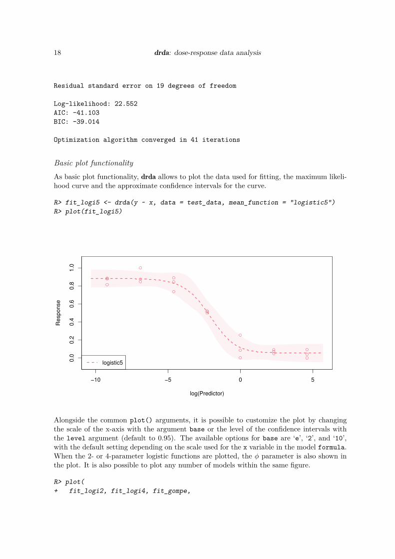
As basic plot functionality, drda allows to plot the data used for Ątting, the maximum likeli-hood curve and the approximate conĄdence intervals for the curve.
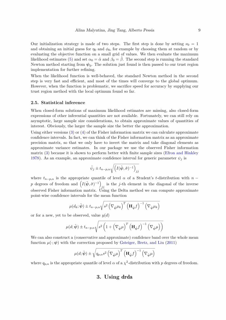
R> fit_logi5 <- drda(y ~ x, data = test_data, mean_function = "logistic5")
R> plot(fit_logi5)
log(Predictor)
Response
−10 −5 0 5
0.0
0.2
0.4
0.6
0.8
1.0
logistic5
Alongside the common plot() arguments, it is possible to customize the plot by changingthe scale of the x-axis with the argument base or the level of the conĄdence intervals withthe level argument (default to 0.95). The available options for base are ŚeŠ, Ś2Š, and Ś10Š,with the default setting depending on the scale used for the x variable in the model formula.When the 2- or 4-parameter logistic functions are plotted, the ϕ parameter is also shown inthe plot. It is also possible to plot any number of models within the same Ągure.
R> plot(
+ fit_logi2, fit_logi4, fit_gompe,

Alina Malyutina, Jing Tang, Alberto Pessia 19
+ base = "10", level = 0.9,
+ xlim = c(-10, 5), ylim = c(-0.1, 1.1),
+ xlab = "Dose", ylab = "Relative viability",
+ legend = c("2-param logistic", "4-param logistic", "Gompertz")
+ )
Dose
Rela
tive
via
bili
ty
10−4
10−3
10−2
10−1
100
101
102
0.0
0.2
0.4
0.6
0.8
1.0
2−param logistic
4−param logistic
Gompertz
Area-based metrics
To obtain a measure of treatment efficacy, functions nauc() and naac() compute respectivelythe normalized area under the curve and above the curve. Since our example data refers toviability data, we use here the NAAC measure: the closer the value to 1 the better thetreatment effect.
R> naac(fit_logi4)
[1] 0.6219635
To allow the values to be comparable between different compounds and/or studies, the func-tion sets a hard constraint on both the x and y variables (see Section 3.1). However, theintervals can be easily changed if needed.
R> naac(fit_logi4, xlim = c(-2, 2), ylim = c(0.1, 0.9))
[1] 0.9062705
20 drda: dose-response data analysis
Relative error
Statistic drda DoseFinding drc nplr
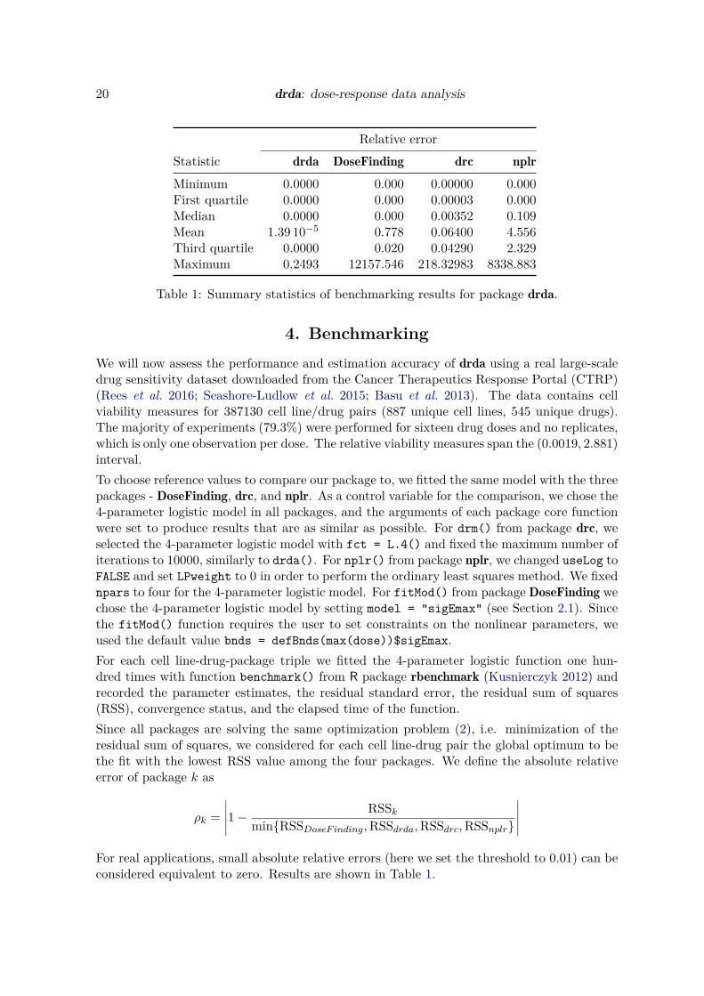
Minimum 0.0000 0.000 0.00000 0.000First quartile 0.0000 0.000 0.00003 0.000Median 0.0000 0.000 0.00352 0.109Mean 1.39 10−5 0.778 0.06400 4.556Third quartile 0.0000 0.020 0.04290 2.329Maximum 0.2493 12157.546 218.32983 8338.883
Table 1: Summary statistics of benchmarking results for package drda.
4. Benchmarking
We will now assess the performance and estimation accuracy of drda using a real large-scaledrug sensitivity dataset downloaded from the Cancer Therapeutics Response Portal (CTRP)(Rees et al. 2016; Seashore-Ludlow et al. 2015; Basu et al. 2013). The data contains cellviability measures for 387130 cell line/drug pairs (887 unique cell lines, 545 unique drugs).The majority of experiments (79.3%) were performed for sixteen drug doses and no replicates,which is only one observation per dose. The relative viability measures span the (0.0019, 2.881)interval.
To choose reference values to compare our package to, we Ątted the same model with the threepackages - DoseFinding, drc, and nplr. As a control variable for the comparison, we chose the4-parameter logistic model in all packages, and the arguments of each package core functionwere set to produce results that are as similar as possible. For drm() from package drc, weselected the 4-parameter logistic model with fct = L.4() and Ąxed the maximum number ofiterations to 10000, similarly to drda(). For nplr() from package nplr, we changed useLog toFALSE and set LPweight to 0 in order to perform the ordinary least squares method. We Ąxednpars to four for the 4-parameter logistic model. For fitMod() from package DoseFinding wechose the 4-parameter logistic model by setting model = "sigEmax" (see Section 2.1). Sincethe fitMod() function requires the user to set constraints on the nonlinear parameters, weused the default value bnds = defBnds(max(dose))$sigEmax.
For each cell line-drug-package triple we Ątted the 4-parameter logistic function one hun-dred times with function benchmark() from R package rbenchmark (Kusnierczyk 2012) andrecorded the parameter estimates, the residual standard error, the residual sum of squares(RSS), convergence status, and the elapsed time of the function.
Since all packages are solving the same optimization problem (2), i.e. minimization of theresidual sum of squares, we considered for each cell line-drug pair the global optimum to bethe Ąt with the lowest RSS value among the four packages. We deĄne the absolute relativeerror of package k as
ρk =
∣
∣
∣
∣
∣
1 −RSSk
min¶RSSDoseF inding,RSSdrda,RSSdrc,RSSnplr♢
∣
∣
∣
∣
∣
For real applications, small absolute relative errors (here we set the threshold to 0.01) can beconsidered equivalent to zero. Results are shown in Table 1.

Alina Malyutina, Jing Tang, Alberto Pessia 21
Overall, drda is Ćagged as the absolute best Ąt in 90.81% of cases. When we only considerthe cases for which ♣ρk♣ ≤ 0.01, the percentage raises to 99.96% (70.21% for DoseFinding,59.98% for drc, and 43.65% for nplr). When compared directly against the other packages,drda outperforms DoseFinding in 29.78% of the cases (worse for 0.033%), drc in 39.99% ofcases (worse for 0.004%), and nplr in 56.34% of the cases (worse for 0.016%).
The results show that drda provides more accurate, and thus more reliable, estimates of thedose-response relationship. The higher accuracy comes obviously at a computational cost, asmore steps are usually needed for exploring the parameter space. Our data analysis revealsthat fitMOD() and nplr() are the fastest functions to complete the Ąt. It took them lessthan a second to converge 95% of the times (mean of 0.62s and median of 0.61s for fitMOD();mean of 0.91s and median of 0.95s for nplr()). On average drda found the global optimum(or a very close solution) in 14.45 seconds (median of 9.6s). For completeness, drm() had anaverage of 9.87 seconds and a median of 3.27 seconds.
5. Summary and discussion
In this paper, we have introduced the drda package, aimed at evaluating dose-response rela-tionship to advance our understanding of biological processes or pharmacological safety. Thesetypes of experiments are of high importance in drug discovery, as they establish an essentialstep for subsequent therapeutic advances. An appropriate interpretation of the experimentaldata is grounded on a reliable estimation of the dose-response relationship. Therefore, it isimperative to provide advanced optimization methods that allow more accurate estimationof dose-response parameters, and the assessment of their statistical signiĄcance.
One of the main limitations of most optimization procedures is their convergence to localsolutions. The basic quasi-Newton methods applied to logistic curve Ątting are sensitive tothe selection of a starting point and to cases when data is non-informative. Our packageeffectively overcomes the convergence problem as we implement a Newton method with atrust region to achieve global convergence and improve it further with a double-step startingpoint initialization. The drda optimization routine also relies on analytical gradient andHessian to avoid numerical approximations. The package allows a user to further evaluatethe model Ątness further via the assessment of conĄdence intervals of the estimates, modelcomparisons, and advanced plot options.
We have compared our package with the three state-of-the-art packages - DoseFinding, drc,and nplr. Using a large-scale drug screening dataset, we have shown that drda has clearlyoutperformed the other three packages in terms of accuracy. Despite the fact that our pack-age is on average slower than the other three packages, its gain in accuracy is a favorablecompromise. For most, if not all, experimental applications, accuracy has a higher priority.The package is currently completely implemented in base R, therefore there are still many op-portunities for improving its performance, by, for example, refactoring core critical functionsin C or improving further the algorithm initialization. If a researcher is looking for a pack-age providing improved accuracy at a relatively low speed-cost, drda might provide a viableoption. The package can be downloaded from https://github.com/albertopessia/drda.
22 drda: dose-response data analysis
Acknowledgments
We thank CSC, the Finnish IT center for science, for the computational resources used toperform the simulations.
Research is supported by the European Research Council (ERC) starting grant, No 716063(DrugComb: Informatics approaches for the rational selection of personalized cancer drugcombinations).
References
Abramowitz M, Stegun IA (1965). Handbook of Mathematical Functions: with Formulas,
Graphs, and Mathematical Tables. Universitext, ninth reprint edition. Dover Publications,Mineola, NY, USA. ISBN 978-0-486-61272-0.
Akaike H (1974). ŞA new look at the statistical model identiĄcation.Ť IEEE Transactions on
Automatic Control, 19(6), 716Ű723. doi:10.1109/TAC.1974.1100705.
Armijo L (1966). ŞMinimization of functions having Lipschitz continuous Ąrst partial deriva-tives.Ť PaciĄc Journal of mathematics, 16(1), 1Ű3. doi:10.2140/pjm.1966.16.1.
Basu A, Bodycombe NE, Cheah JH, Price EV, Liu K, Schaefer GI, Ebright RY, StewartML, Ito D, Wang S, Bracha AL, Liefeld T, Wawer M, Gilbert JC, Wilson AJ, StranskyN, Kryukov GV, Dancik V, Barretina J, Garraway LA, Hon CSY, Munoz B, Bittker JA,Stockwell BR, Khabele D, Stern AM, Clemons PA, Shamji AF, Schreiber SL (2013). ŞAninteractive resource to identify cancer genetic and lineage dependencies targeted by smallmolecules.Ť Cell, 154(5), 1151Ű1161. doi:10.1016/j.cell.2013.08.003.
Bonnans JF, Gilbert JC, Lemarechal C, Sagastizábal CA (2006). Numerical optimization:
Theoretical and practical aspects. Universitext, second edition. Springer-Verlag, Heidelberg,Germany. ISBN 978-3-540-35445-1.
Bornkamp B, Pinheiro J, Bretz F (2019). DoseFinding: Planning and analyzing dose Ąnding
experiments. R package version 0.9-17, URL https://cran.r-project.org/package=
DoseFinding.
Commo F, Bot BM (2016). nplr: N-Parameter logistic regression. R package version 0.1-7,URL https://cran.r-project.org/package=nplr.
Efron B, Hinkley DV (1978). ŞAssessing the accuracy of the maximum likelihood estimator:Observed versus expected Fisher information.Ť Biometrika, 65(3), 457Ű483. doi:10.1093/
biomet/65.3.457.
Fletcher R (2000). Practical methods of optimization. Second edition. John Wiley & Sons,Chichester, UK. ISBN 978-0-471-49463-8.
Gsteiger S, Bretz F, Liu W (2011). ŞSimultaneous conĄdence bands for nonlinear regressionmodels with application to population pharmacokinetic analyses.Ť Journal of Biopharma-
ceutical Statistics, 21(4), 708Ű725. doi:10.1080/10543406.2011.551332.

Alina Malyutina, Jing Tang, Alberto Pessia 23
Kusnierczyk W (2012). rbenchmark: Benchmarking routine for R. R package version 1.0.0,URL https://CRAN.R-project.org/package=rbenchmark.
Liu DC, Nocedal J (1989). ŞOn the limited memory BFGS method for large scale optimiza-tion.Ť Mathematical programming, 45(1), 503Ű528. doi:10.1007/bf01589116.
Luenberger DG, Ye Y (2008). Linear and nonlinear programming. International Series inOperations Research & Management Science, third edition. Springer-Verlag, New York,NY, USA. ISBN 978-0-387-74502-2.
Macdougall J (2006). Analysis of dose-response studies Ů Emax model, pp. 127Ű145. Springer-Verlag, New York, NY, USA. ISBN 978-0-387-33706-7.
Mogensen PK, Riseth AN (2018). ŞOptim: A mathematical optimization package for Julia.ŤJournal of Open Source Software, 3(24), 615. doi:10.21105/joss.00615.
Nocedal J, Wright SJ (2006). Numerical optimization. Springer Series in Operations Researchand Financial Engineering, second edition. Springer-Verlag, New York, NY, USA. ISBN978-0-387-30303-1.
Rees MG, Seashore-Ludlow B, Cheah JH, Adams DJ, Price EV, Gill S, Javaid S, Coletti ME,Jones VL, Bodycombe NE, Soule CK, Alexander B, Li A, Montgomery P, Kotz JD, HonCSY, Munoz B, Liefeld T, Dančík V, Haber DA, Clish CB, Bittker JA, Palmer M, WagnerBK, Clemons PA, Shamji AF, Schreiber SL (2016). ŞCorrelating chemical sensitivity andbasal gene expression reveals mechanism of action.Ť Nature Chemical Biology, 12(2), 109Ű116. doi:10.1038/nchembio.1986.
Richards FJ (1959). ŞA Ćexible growth function for empirical use.Ť Journal of Experimental
Botany, 10(2), 290Ű301. doi:10.1093/jxb/10.2.290.
Ritz C, Baty F, Gerhard D (2015). ŞDose-response analysis using R.Ť PLoS ONE,10(e0146021), 1Ű13. doi:10.1371/journal.pone.0146021.
Schwarz G (1978). ŞEstimating the dimension of a model.Ť The Annals of Statistics, 6(2),461Ű464. doi:10.1214/aos/1176344136.
Seashore-Ludlow B, Rees MG, Cheah JH, Cokol M, Price EV, Coletti ME, Jones V, Body-combe NE, Soule CK, Gould J, Alexander B, Li A, Montgomery P, Wawer MJ, KuruN, Kotz JD, Hon CSY, Munoz B, Liefeld T, Dančík V, Bittker JA, Palmer M, Brad-ner JE, Shamji AF, Clemons PA, Schreiber SL (2015). ŞHarnessing connectivity in alarge-scale small-molecule sensitivity dataset.Ť Cancer Discovery, 5(11), 1210. doi:
10.1158/2159-8290.CD-15-0235.
Sorensen DC (1982). ŞNewtonŠs method with a model trust region modiĄcation.Ť SIAM
Journal on Numerical Analysis, 19(2), 409Ű426. doi:10.1137/0719026.
Steihaug T (1983). ŞThe conjugate gradient method and trust regions in large scale optimiza-tion.Ť SIAM Journal on Numerical Analysis, 20(3), 626Ű637. doi:10.1137/0720042.

24 drda: dose-response data analysis
Affiliation:
Alina Malyutina, Jing Tang, Alberto PessiaResearch Program in Systems Oncology (ONCOSYS)Faculty of MedicineUniversity of HelsinkiHaartmaninkatu 800290 Helsinki, FinlandE-mail:[email protected]
URL:helsinki.Ą/en/researchgroups/network-pharmacology-for-precision-medicine/software