Embed Size (px)
Citation preview

A pooled fund project administered by the Minnesota Department of Transportation
Authors: Hyunjun Oh, William Likos, Tuncer Edil
Drainability of Base Aggregate and Sand
Report No. NRRA202107

To request this document in an alternative format, such as braille or large print, call 651-366-4718 or 1-800-657-3774 (Greater Minnesota) or email your request to [email protected]. Please request at least one week in advance.

Technical Report Documentation Page 1. Report No. 2. 3. Recipients Accession No.
NRRA202107
4. Title and Subtitle 5. Report Date
Drainability of Base Aggregate and Sand August 2021 6.
7. Author(s) 8. Performing Organization Report No.
Hyunjun Oh, William J. Likos, Tuncer B. Edil 9. Performing Organization Name and Address 10. Project/Task/Work Unit No.
Department of Civil and Environmental Engineering University of Wisconsin-Madison 11. Contract (C) or Grant (G) No. Madison, WI 53706
(c)1003328 (wo)02 12. Sponsoring Organization Name and Address 13. Type of Report and Period Covered
Minnesota Department of Transportation Office of Research & Innovation
Final Report 14. Sponsoring Agency Code
395 John Ireland Boulevard, MS 330 St. Paul, Minnesota 55155-1899 15. Supplementary Notes
https://www.mndot.gov/research/reports/2021/NRRA202107.pdf 16. Abstract (Limit: 250 words)
Poor drainage of roadway base materials can lead to increased pore water pressure, reduction of strength and
stiffness, and freeze-thaw damage. Drainability is dependent on soil/aggregate physical properties that affect
water flow and retention in the porous matrix, notably including particle-size distribution, particle shape, fines
content, and density or porosity. The objective of this project was to quantitatively assess permeability and water
retention characteristics of soil and aggregates applicable to pavement applications and to evaluate and derive
predictive equations for indirect estimation of these properties. Samples of 16 materials used in transportation
geosystems were obtained and laboratory tests were conducted to determine grain size distribution, index
properties, saturated hydraulic conductivity, and soil-water characteristic curves. Results were analyzed to
examine applicability of estimation equations available in the literature and to develop dataset-specific equations
for the specific suite of materials. Procedures were provided to qualitatively assess base course drainability as
“excellent,” “marginal,” and “poor” from grain size properties, thereby offering rationale to reduce pavement life-
cycle costs, improve safety, realize material cost savings, and reduce environmental impacts.
17. Document Analysis/Descriptors 18. Availability Statement
Permeability coefficient, permeability, drainage, pavements, No restrictions. Document available from:
base course (pavements) National Technical Information Services,
Alexandria, Virginia 22312
19. Security Class (this report) 20. Security Class (this page) 21. No. of Pages 22. Price
Unclassified Unclassified 157 n/a

DRAINABILITY OF BASE AGGREGATE AND SAND
FINAL REPORT
Prepared by:
Hyunjun Oh
William J. Likos
Tuncer B. Edil
Department of Civil and Environmental Engineering
University of Wisconsin-Madison
August 2021
Published by:
Minnesota Department of Transportation
Office of Research & Innovation
395 John Ireland Boulevard, MS 330
St. Paul, Minnesota 55155-1899
This report represents the results of research conducted by the authors and does not necessarily represent the views or policies
of the Minnesota Department of Transportation or University of Wisconsin-Madison. This report does not contain a standard or
specified technique.
The authors, the Minnesota Department of Transportation, and University of Wisconsin-Madison do not endorse products or
manufacturers. Trade or manufacturers’ names appear herein solely because they are considered essential to this report.

ACKNOWLEDGMENTS
Financial support from the National Road Research Alliance (NRRA) is acknowledged and appreciated
(Permeability of Base Aggregate and Sand; Contract number 1003328.). The Minnesota, Wisconsin, and
Missouri departments of transportation collaborated in the selection and obtainment of the test
samples. Jie Yin, faculty in Civil Engineering and Mechanics at Jiangsu University, China, and Tyler Klink,
graduate research assistant at the Department of Civil and Environmental Engineering, University of
Wisconsin-Madison, contributed to the literature review. These efforts are gratefully acknowledged.

TABLE OF CONTENTS
CHAPTER 1: Introduction .......................................................................................................................... 1
1.1 Problem Statement .................................................................................................................................... 1
1.2 Research Benefits ....................................................................................................................................... 1
1.3 Methodology .............................................................................................................................................. 2
1.3.1 Literature Review ................................................................................................................................ 2
1.3.2 Laboratory Testing .............................................................................................................................. 2
1.3.3 Analysis ............................................................................................................................................... 3
1.4 Background ................................................................................................................................................. 4
1.4.1 Drainability as an Unsaturated Soils Problem..................................................................................... 4
1.4.2 Hydraulic Conductivity and Permeability (Lu and Likos, 2004) ........................................................... 5
1.4.3 Soil Water Characteristic Curve (Lu and Likos, 2004) ......................................................................... 6
1.4.4 Soil Water Characteristic Curve Modeling (Lu and Likos, 2004) ......................................................... 8
1.4.5 The van Genuchten (1980) SWCC Model (Lu and Likos, 2004) ......................................................... 10
1.4.6 The Hydraulic Conductivity Function (Lu and Likos, 2004) ............................................................... 10
1.4.7 Hydraulic Conductivity Function Modeling ....................................................................................... 14
1.4.8 Base Course Drainability ................................................................................................................... 14
CHAPTER 2: Materials and Methods ........................................................................................................ 16
2.1 Materials................................................................................................................................................... 16
2.2 Grain Size Analysis .................................................................................................................................... 21
2.3 Hydraulic Conductivity Testing ................................................................................................................. 23
2.4 Soil-Water Characteristic Curve Testing ................................................................................................... 26
CHAPTER 3: Experimental Results ........................................................................................................... 28
3.1 Hydraulic Conductivity ............................................................................................................................. 28
3.2 Soil-Water Characteristic Curves .............................................................................................................. 30
CHAPTER 4: Analysis ............................................................................................................................... 33

4.1 Hydraulic Conductivity and Index Properties ........................................................................................... 33
4.2 Soil Water Characteristic Curves and Index Properties ............................................................................ 38
4.3 Field Capacity, Effective Porosity and Minimum Saturation .................................................................... 40
4.4 Hydraulic Conductivity and SWCC Parameters ........................................................................................ 42
4.5 Hydraulic Conductivity Functions ............................................................................................................. 44
4.6 Saturated Hydraulic Conductivity Models ................................................................................................ 45
4.6.1 Models from the Literature .............................................................................................................. 45
4.6.2 Dataset Specific Models .................................................................................................................... 52
4.6.3 Performance Evaluation and Improvement of D10-Based Equation using Data from the Literature54
4.7 Soil-Water Characteristic Curve Models .................................................................................................. 57
4.7.1 Benson et al (2014) ........................................................................................................................... 57
4.7.2 Dataset Specific Models .................................................................................................................... 61
CHAPTER 5: Conclusions and Recommendations ..................................................................................... 66
5.1.1 Summary and Key Findings ............................................................................................................... 66
5.1.2 Qualitative Material Rating System for Base Course Drainability .................................................... 67
5.1.3 Recommendation 1: Qualitative Material Rating Based on Direct Measurements of Permeability
and Water Retention ......................................................................................................................... 68
5.1.4 Recommendation 2: Qualitative Material Rating Based on Grain Size Indices ................................ 69
5.1.5 Recommendation 3: Qualitative Material Rating Based on Percent Fines ....................................... 72
5.1.6 Comparison of Qualitative Drainability Approaches and Implementation ...................................... 73
REFERENCES ........................................................................................................................................... 75
APPENDIX A Case History Review
APPENDIX B Relationships between Minimum Saturations and Index Properties
APPENDIX C Empirical and Theoretical Relations for Estimating Hydraulic Conductivity
APPENDIX D Comparisons of Saturated Hydraulic Conductivities for 16 Samples Obtained from Experiments
and Estimations

LIST OF FIGURES
Figure 1.1 Schematic illustration of a pavement base system in the unsaturated condition. Pore pressure
at hydrostatic equilibrium varies from negative values (suction) above the water table to positive values
below the water table. Corresponding degree of saturation of the base material is quantified by the soil-
water characteristic curve. ...................................................................................................................... 5
Figure 1.2 Conceptual SWCC for coarse soil showing capillary, funicular, and pendular saturation regimes
(Lu and Likos, 2004). ................................................................................................................................ 7
Figure 1.3 Conceptual SWCC along hysteretic wetting and drying paths showing key points on the curve
used for modeling. .................................................................................................................................. 9
Figure 1.4 Conceptual distributions of pore water and pore air in a cross-sectional area of rigid soil
matrix during incremental desaturation process (Lu and Likos, 2004) .................................................... 12
Figure 1.5 (a) Conceptual soil-water characteristic curve and (b) hydraulic conductivity function
corresponding to saturation conditions for a rigid soil matrix shown in Figure 1.4 (Lu and Likos, 2004).. 13
Figure 2.1 17 coarse-grained samples: (a) 1 (SP-SM), (b) 2 (SW-SM), (c) 3 (SM), (d) 4 (GM), (e) 5 (SP), (f) 6
(GP), (g) 7 (SW), (h) 8 (SP), (i) 9 (GP), (j) 10 (SP), (k) 15 (GM), (l) 16 (SM), (m) A1 (GW-GM), (n) A2 (GP), (o)
A3 (SP), (p) A4 (GW-GM), and (q) A5 (GW-GM) ...................................................................................... 21
Figure 2.2 Particle-size distribution curves for 17 samples ..................................................................... 22
Figure 2.3 Constant head hydraulic conductivity test apparatus: (a) schematic and (b) photograph ....... 24
Figure 2.4 Large-scale hanging column apparatus: (a) schematic and (b) photograph ............................ 27
Figure 3.1 Hydraulic conductivity testing results for: (a) seven gravels and (b) nine sandy soils .............. 28
Figure 3.2 Soil-water characteristic curves for: (a) gravels regarding volumetric water content, (b) gravels
regarding degree of saturation, (c) sandy soils regarding volumetric water content, and (d) sandy soils
regarding degree of saturation. ............................................................................................................. 32
Figure 4.1 Relationships between experimentally obtained Ksat,avg values and (a) D10 in full range, (b) D10
in small range except three outliers, (c) D30, (d) multivariable on D10 and D30, (e) D50, and (f) D60............ 36
Figure 4.2 Relationships between experimentally measured Ksat,avg and (a) %retained gravels, (b) % fines,
(c) Cu, and (d) γd ..................................................................................................................................... 38
Figure 4.3 Relationship between air-entry pressure and uniformity coefficient ...................................... 39
Figure 4.4 Relationships between air-entry pressure and van Genuchten parameters: (a) α and (b) n.... 40
Figure 4.5 Relationship between 16 minimum saturations and % fines .................................................. 42

Figure 4.6 Relationships between van Genuchten parameters of Ksat,avg for 15 samples: (a) relationship
between van Genuchten parameter α and average Ksat,avg and (b) relationship between van Genuchten
parameter n and average Ksat,avg............................................................................................................. 43
Figure 4.7 Hydraulic conductivity functions using van Genuchten (1980) approach: (a) unsaturated
hydraulic conductivity functions for six gravels, and (b) unsaturated hydraulic conductivity functions for
nine sandy soils. .................................................................................................................................... 45
Figure 4.8 Comparisons of experimentally measured and estimated Ksat values for (a) 13 samples and (b)
11 samples ............................................................................................................................................ 48
Figure 4.9 Comparisons of estimated and measured Ksat for 11 samples excluding #4, #6, #9, A2, and A4
using (a) Alyamani and Sen (1993), (b) Beyer (1964), (c) Chapuis et al. (2005), (d) Harleman et al. (1963),
(e) Hazen-Original (1892), (f) Hazen-Modified, (g) Kozeny (1953), (h) Kozeny-Carman (Kozeny 1927,
1953; Carman1937, 1956), (i) Salarashayeri and Siosemarde (2012), (j) Sauerbrei (1932), (k) Slichter
(1899), (l) Terzaghi (1925), and (m) U.S. Bureau of Reclamation ............................................................ 51
Figure 4.10 Comparisons of Ksat values obtained from experiments and estimations using regression
equations based on (a) D10, (b) D30, (c) multivariable on D10 and D30, (d) D50, and (e) D60 ........................ 53
Figure 4.11 Comparisons of Ksat measurements and estimations obtained using eq. (4.2) for base
materials: (a) in full range and (b) in small range excluding #6, #9, and A2 ............................................. 56
Figure 4.12 Relationship between Ksat and D10 of 16 samples and recycled base materials ..................... 56
Figure 4.13 Comparisons of Ksat measurements and estimations obtained using eq. (4.7) for base
materials: (a) in full range and (b) in small range excluding #6, #9, and A2 ............................................. 57
Figure 4.14 Deriving new regression equations using experimental results of 15 samples: (a) relationship
between D60 and van Genuchten parameter α, (b) relationship between D60 and van Genuchten
parameter n, (c) relationship between Cu and normalized α, and (d) relationship between Cu and
normalized n ......................................................................................................................................... 59
Figure 4.15 Comparisons of van Genuchten parameters obtained from experiments and estimations: (a)
comparison of α parameters, (b) comparison of n parameters. ............................................................. 60
Figure 4.16 Relationships between experimentally obtained van Genuchten fitting parameters and index
properties: (a) relationship between α and D10, (b) relationship between n and D10, (c) relationship
between α and D30, (d) relationship between n and D30, (e) relationship between α and D50, (f)
relationship between n and D50, (g) relationship between α and γd, and (h) relationship between n and γd
.............................................................................................................................................................. 62
Figure 4.17 Comparisons of van Genuchten parameters obtained from experiments and pedotransfer
functions based on: (a) D10 for α parameter, (b) D10 for n parameter, (c) D30 for α parameter, (d) D30 for n

parameter, (e) D50 for α parameter, (f) D50 for n parameter, (g) γd for α parameter, and (h) γd for n
parameter ............................................................................................................................................. 65
Figure 5.1 Relations among hydraulic conductivity, minimum saturation and percent fines with
boundaries for “excellent” and “marginal” drainability. ......................................................................... 72

LIST OF TABLES
Table 2.1 Nominal designation and description of 17 soil samples ......................................................... 16
Table 2.2 Index properties of 17 samples ............................................................................................... 22
Table 2.3 Dry unit weight of the soil specimens in Ksat and SWCC tests................................................... 25
Table 3.1 Hydraulic conductivity testing results for seven gravels .......................................................... 29
Table 3.2 Hydraulic conductivity testing results for nine sandy soils ....................................................... 29
Table 3.3 Summary of SWCC parameters ............................................................................................... 32
Table 4.1 Index properties and dry unit weight (γd) of the soil specimens in permeameter .................... 33
Table 4.2 Field capacities, effective porosities, and minimum saturations for 16 samples ...................... 41
Table 4.3 Summary of Ksat,avg testing results and van Genuchten fitting parameters ............................... 43
Table 4.4 Summary of saturated hydraulic conductivity estimated using 13 applicable empirical
equations .............................................................................................................................................. 47
Table 4.5 Experimentally measured Ksat and D10 data of recycled base materials obtained from the
literature ............................................................................................................................................... 55
Table 5.1 Recommended material parameters for qualitative drainability assessment of pavement base
course materials .................................................................................................................................... 68
Table 5.2 Qualitative performance rating of materials based on measured permeability and water
retention ............................................................................................................................................... 69
Table 5.3 Qualitative performance rating of materials based on permeability and water retention
estimated from grain size distribution ................................................................................................... 70
Table 5.4 Qualitative performance rating of materials based on percent fines ....................................... 73
Table 5.5 Comparison of drainability assessments following three recommended approaches .............. 74

EXECUTIVE SUMMARY
Drainability is a material property that describes fluid flow and retention in porous material and is a
significant consideration in the design and long-term performance of pavement systems. Poor drainage
in roadway base materials, for example, can lead to problems including increased pore water pressure,
reduction of strength and stiffness, and freeze-thaw damage.
Base course drainability is dependent on soil/aggregate physical properties that affect water flow and
retention in the porous matrix, notably including particle-size distribution, particle shape, fines content,
and density or porosity. For unsaturated soil systems, both hydraulic conductivity and soil-water
retention characteristics are necessary to predict drainage behavior. In lieu of direct measurements of
these properties, empirical and theoretical relations are available and are often used to estimate them
from more easily obtained surrogate properties such as gradation and porosity. The accuracy and
applicability of such estimations, however, are uncertain and are often limited to the specific datasets
from which they were obtained.
The objective of this project is to provide rationale to assess the drainability of coarse soil/aggregate
materials applicable to pavement base course applications. Emphasis is placed on saturated hydraulic
conductivity and water retention, including evaluation of existing predictive equations for indirect
estimation of these properties from surrogate material properties (e.g., grain size distribution) and the
development of new correlation equations for the materials examined here.
Samples of 16 representative materials were obtained from National Road Research Alliance (NRRA)
stakeholders, including materials that are generally classified as gravels (7 samples) and sands (9
samples). Laboratory tests were conducted to determine grain size distribution, grain size index
properties, saturated hydraulic conductivity (Ksat), and soil-water characteristic curves (SWCCs). Key
findings from the experimental program included the following:
1) Measured Ksat of the 9 sandy materials is independent of hydraulic gradient (i) typical of field
conditions for pavement base applications (0.25 < i < 2.0). Measured Ksat of the 7 gravels
systematically decreases with increasing hydraulic gradient, potentially due to migration of fines
and the effects of turbulent flow.
2) Ksat for all the materials generally increases as % gravels and particle diameters corresponding to
10%, 30%, 50%, and 60% finer (D10, D30, D50, and D60, respectively) increases. Ksat generally
increases as % fines and dry unit weight (γd) of compacted samples decreases.
3) Ksat slightly increases with a decrease in uniformity coefficient (Cu), but the relationship is not
significantly correlated. Air-entry pressure determined from the measured soil-water
characteristic curves increases with an increase in Cu.
4) The van Genuchten (1980) SWCC parameters (α and n) increase with increases in D10, D30, D50,
D60, and % retained gravels and with decreases in % fines, Cu, and γd. Comparisons among the
experimentally measured Ksat values and the van Genuchten α and n parameters show a
proportional relationship.
5) Effective (drainable) porosities for the 16 samples ranges from 0.09 to 0.36 with an average of
0.24. Corresponding minimum saturation (Smin), which is achieved by gravity, ranges from 0.01

to 0.69 with an average of 0.25. These results are comparable to typical values for similar
materials in the literature.
Test results were analyzed to examine the accuracy and applicability of equations available in the
literature for estimating Ksat and SWCC parameters and to develop dataset-specific equations for the
suite of materials tested here. This analysis showed:
1) Estimated Ksat for materials that classified as poorly graded gravel (GP) are significantly higher
than the experimentally measured Ksat values. Measured Ksat for a subset of samples that
excludes the gravels is generally well estimated using the Harleman et al. (1963), Sauerbrei
(1932), and Chapuis (2004) empirical equations.
2) New dataset-specific regression equations to estimate Ksat are derived using the experimentally
obtained Ksat and grain size index properties (D10, D30, D50, D60). Measured Ksat values that are
overestimated using the existing equations are reasonably estimated with the new equations,
particularly using equations based on D10 and D30.
3) The van Genuchten (1980) SWCC fitting parameters α and n are estimated using regression
equations following procedures developed by Benson et al. (2014) for clean sands. Equations
based on D30 and Cu show the best performance.
A qualitative rating system for assessing base course drainability is provided by setting criteria for
saturated hydraulic conductivity (Ksat) and minimum saturation (Smin) at field capacity. The rating system
may be used to qualitatively assess the drainability of candidate base course material as “excellent,”
“marginal,” or “poor.” Three approaches to obtain hydraulic conductivity and water retention
characteristics are recommended:
1) Recommendation 1: Direct measurement of Ksat and Smin from laboratory tests.
2) Recommendation 2: Indirect estimation of Ksat and Smin from correlation to grain size
parameters. Application of this approach requires a measurement of grain size distribution to
obtain D30 and Cu using mechanical sieve analysis.
3) Recommendation 3: Indirect assessment of drainability from measured percent fines.
Application of this approach requires a measurement percent passing the #200 sieve using
mechanical sieve analysis.
While rigorous drainability analysis of in-situ pavement systems requires knowledge of material
properties, pavement system design, and site environmental conditions, the approaches recommended
in this research offer a rationale for material selection and quality assessment that will reduce pavement
life-cycle costs, improve safety, realize material cost savings, and reduce environmental impacts.

1
CHAPTER 1: INTRODUCTION
1.1 PROBLEM STATEMENT
Geosystems such as roadway base course and retaining wall backfills are designed to quickly drain
porewater to minimize elevated pore pressure, minimize freeze-thaw damage, and prevent loss of shear
strength and stiffness. Requirements for drainability vary depending on the specific requirements of the
structure. Simple and reliable tools capable of qualitatively estimating drainability for common
aggregate types used in transportation infrastructure can be useful in material selection and design and
to ensure longer-term performance.
Pavement base course layers are unsaturated under most field conditions, and thus both hydraulic
conductivity (K) and soil-water retention characteristics are necessary to evaluate drainage behavior.
Hydraulic conductivity and water retention characteristics, however, are not typically measured or used
explicitly in design. In lieu of direct measurements of these properties, empirical and theoretical
relations are available and often used to estimate saturated hydraulic conductivity (Ksat) and the soil-
water characteristic curve (SWCC) from more easily obtained surrogate material properties, notably
including grain size distribution and density, porosity, or void ratio. The accuracy and applicability of
such estimations, however, are uncertain and often limited to the specific datasets from which they are
obtained.
The objective of this study was to quantitatively determine hydraulic conductivity and water retention
characteristics for representative coarse-grained soil/aggregate materials applicable to pavement base
course applications and to evaluate and derive predictive equations for indirectly estimating Ksat and the
SWCC. Samples of 16 materials were obtained from National Road Research Alliance (NRRA)
stakeholders and tests were conducted to determine grain size distribution, grain size index properties
(e.g., D10, D30, D50, D60, Cu), Ksat and SWCCs. Test results were analyzed to examine the accuracy and
applicability of existing equations for estimating Ksat and SWCC parameters and to develop dataset-
specific equations for the suite of test materials obtained here.
1.2 RESEARCH BENEFITS
Anticipated research benefits of the project include the following:
Reduced Life-Cycle Costs
Improved Safety
Material Cost Savings
Construction Savings
Reduced Environmental Impacts

2
Drainability of pavement base and subbase is one of the main considerations in designing pavement
systems and in the post-construction performance and safety of the pavement structure. Poor drainage
of roadway base course and associated elevation of pore water pressure in the material will reduce
stiffness and strength, which can lead to surface rutting and cracking, and can lead to damage from
freeze/thaw processes. This can significantly reduce the pavement life cycle, increase maintenance
costs, and lead to poor roadway performance and safety. Developing more robust methods to assess
material drainability from surrogate material properties will thus reduce pavement life-cycle costs and
improve safety. Improved empirical approaches to estimate drainability will also potentially realize
material cost savings, construction savings, and reduce environmental impacts (e.g., material sourcing
and transport) by providing rationale to allow a wider range of locally available materials to be
considered for construction. Implementation of the results of this research will lead to improvement of
safety and reduction of maintenance and engineering costs associated with repairing roadways.
1.3 METHODOLOGY
1.3.1 Literature Review
A literature review focused on select case studies related to performance evaluation of geosystems such
as pavement base course, subbase, and retaining wall backfills. Case histories focused on evaluating
subsurface drainage systems based on literature reviews, surveys, experiments, numerical modeling,
and statistical analyses, with emphasis placed on research on pavement systems performed by the
Minnesota Department of Transportation (MnDOT) and partner entities. Synthesis of the case studies
provides a practical background for the project. Results from the case study literature review are
provided in Appendix A.
A second literature review was conducted to synthesize information on permeability of coarse
aggregates and sands, with emphasis on existing methods for estimating permeability from other index
properties. Approaches were subdivided into those that correlate saturated hydraulic conductivity to i)
grain size distribution, ii) void ratio, iii) compaction level, iv) fines content, and v) material type. Results
from this portion of the literature review are provided in Appendix C.
1.3.2 Laboratory Testing
A suite of coarse-grained samples was obtained from NRRA stakeholders to represent a range of
materials that have been used in (or have been considered for use in) transportation infrastructure
systems. Materials included 17 discrete samples ranging from poorly graded sand (SP), silty sand (SM),
well-graded sand (SW), poorly graded gravel (GP), silty gravel (GM), to well-graded gravel (GW). (16 of
the samples were used in the project). Materials were selected in partnership with NRRA
representatives from the Minnesota (MnDOT), Missouri (MoDOT), and Wisconsin (WisDOT)
Departments of Transportation.

3
Particle-size distributions of the samples were determined by standard sieve analysis (ASTM D422) and
hydrometer analysis (ASTM D7928). Materials were classified according to the ASTM D2487 unified soil
classification system (USCS). Saturated hydraulic conductivity values (Ksat) were determined for samples
compacted in a rigid-walled permeameter at dry density (𝛾𝑑) ranging from 15.6 kN/m3 to 20.1 kN/m3
using the constant head method (ASTM D2434). Hydraulic conductivity testing was repeated using five
hydraulic gradients (i = 0.25, 0.5, 1.0, 1.5, and 2.0) selected to represent a range of field conditions
typical for pavement base course applications and to quantify any effects of applied hydraulic gradient
on measured conductivity (e.g., from particle migration or turbulent effects). Average Ksat values from
tests spanning the range of gradients were calculated for subsequent modeling and analysis.
Soil water characteristic curves (SWCCs) were measured using the hanging column test apparatus (ASTM
D6836). Samples for SWCC testing were compacted to dry density values within 1% of values used in the
hydraulic conductivity tests. SWCCs were obtained along primary drying curves initiating at zero matric
suction () and full saturation (S) to matric suction of approximately 100 kPa. The highest suction
corresponded to degree of saturation ranging from near zero to 30%, depending on the material.
Measured SWCCs were fit to the commonly adopted van Genuchten (1980) SWCC model using least-
squared regression to calculate model parameters ( and n) used in subsequent analysis.
1.3.3 Analysis
Index properties obtained from the grain size distributions (D10, D30, D50, D60, % fines, % gravel) were
used to evaluate relationships between these properties and measured Ksat values. Air-entry pressures
determined from the SWCC measurements were related to index properties (e.g., grain size uniformity
coefficient, Cu) and to the van Genuchten (1980) model parameters. The SWCC model parameters were
then related to index properties including D10, D50, and % gravel, % fines, Cu, and dry unit weight,
unsaturated Ksat functions, and Ksat values obtained from the hydraulic conductivity measurements. The
SWCCs were also used to evaluate field capacity (θf) and minimum saturation (Smin).
Existing empirical and theoretical methods for estimating hydraulic conductivity identified in the
literature review were assessed for their applicability to the suite of specific materials tested here. The
experimentally obtained Ksat values and index properties were then considered to derive new equations
for estimating Ksat. Finally, a new suite of equations was developed for estimating the van Genuchten
SWCC parameters α and n from particle-size distribution data.
A qualitative rating system for assessing base course drainability is provided by setting criteria for
saturated hydraulic conductivity (Ksat) and minimum saturation (Smin) at field capacity. The rating system
may be used to qualitatively assess the drainability of candidate base course material as “excellent,”
“marginal,” or “poor.” Three approaches to obtain hydraulic conductivity and water retention
characteristics are recommended:
1) Recommendation 1: Direct measurement of Ksat and Smin from laboratory tests.
2) Recommendation 2: Indirect estimation of Ksat and Smin from correlation to grain size
parameters. Application of this approach requires a measurement of grain size distribution to
obtain D30 and Cu using mechanical sieve analysis.

4
3) Recommendation 3: Indirect assessment of drainability from measured percent fines.
Application of this approach requires a measurement percent passing the #200 sieve using
mechanical sieve analysis.
1.4 BACKGROUND
1.4.1 Drainability as an Unsaturated Soils Problem
Figure 1.1 is a conceptual illustration of a pavement base system illustrating the unsaturated state of the
system under typical field conditions. The water table is located at the interface of the base and
subgrade for illustration. Pore pressure in the base material at hydrostatic equilibrium varies from
negative values (suction) above the water table to positive values below the water table. Corresponding
degree of saturation of the base material is quantified by its soil-water characteristic curve. The
existence of negative pressure in the base material contributes to strength and stiffness, thus enhancing
its performance as a structural layer.
If a precipitation (or other wetting) event occurs that introduces water into the system, the pore
pressure profile will shift to toward more positive values as the wetting front passes through the system
until hydrostatic equilibrium is once again achieved, thus reducing effective stress in the material and
reducing corresponding strength and stiffness. The duration of this transient process is controlled by
both the hydraulic conductivity of the unsaturated soil system and the water retention characteristics,
as governed by the soil-water characteristic curve. Materials that do not freely drain (i.e., having low
hydraulic conductivity or high water retention capacity) will maintain elevated pore pressures for a
longer period and, if not fully drained, can be subject to freeze-thaw processes. Full assessment of
material drainability, and system performance, therefore, must take into consideration both the
hydraulic conductivity and water retention characteristics of the material. These material characteristics
depend on the properties of the soil/aggregate grains themselves (e.g., size, size distribution, shape),
their compaction characteristics (e.g., density, void ratio, porosity), and of the permeant fluid (viscosity,
density), and is referred to herein as “drainability.”

5
Figure 1.1 Schematic illustration of a pavement base system in the unsaturated condition. Pore pressure at
hydrostatic equilibrium varies from negative values (suction) above the water table to positive values below the
water table. Corresponding degree of saturation of the base material is quantified by the soil-water
characteristic curve.
1.4.2 Hydraulic Conductivity and Permeability (Lu and Likos, 2004)
Darcy’s law states that the discharge velocity of fluid from a porous medium, v, is linearly proportional
to the gradient in the relevant driving head, h, as follows:
𝑣 = −𝐾∇ℎ (1.1)
where 𝐾 = a proportionality term describing the conductivity of the porous medium [m/s]. The negative
sign preceding the right-hand side of eq. (1.1) indicates that fluid flow occurs from a location of
relatively high total head to a location of relatively low total head. Seepage velocity, vs, which describes
the average actual flow velocity through the pores of the medium, is the discharge velocity divided by
the medium porosity (i.e., vs = v/n).
The proportionality parameter K in eq. (1.1) describes the ability for a specific porous medium under
specific conditions to transmit a specific fluid. For the flow of pore water in soil/aggregate, the driving
gradient is the total hydraulic head and the constant of proportionality is the hydraulic conductivity (K).

6
Discharge velocity is proportional to the viscosity and density of the permeant fluid, being higher for
relatively high density or low viscosity fluids. These proportionalities are captured mathematically as
follows:
𝑣 ∝𝜌𝑔
𝜇 (1.2)
where 𝜌= the fluid density [kg/m3], 𝑔 = gravitational acceleration [m/s2], and = the dynamic (absolute)
fluid viscosity [Ns/m2].
Experimental results and theoretical considerations also reveal that discharge velocity is highly
dependent on pore size and pore-size distribution. Following Poiseuille’s law, the discharge velocity is
proportional to the square of the pore diameter d, or:
𝑣 ∝ 𝑑2 (1.3)
Combining the above two proportionalities with Darcy’s original observation that discharge velocity is
linearly proportional to the total head gradient leads to the following:
𝑣 = −𝐶𝑑2𝜌𝑔
𝜇∇ℎ (1.4)
where 𝐶 = a dimensionless constant related to the geometry of the soil pores. Comparing eq. (1.4) with
eq. (1.1) leads to:
𝐾 = (𝐶𝑑2) (𝜌𝑔
𝜇) (1.5)
If intrinsic permeability, k, is defined as follows:
𝑘 = 𝐶𝑑2 (1.6)
then, together with eq. (1.5), the relationship between intrinsic permeability and hydraulic conductivity
becomes:
𝐾 =𝜌𝑔
𝜇𝑘 (1.7)
Intrinsic permeability, or simply permeability, has units of length squared (m2) and is dependent only on
the pore size, pore geometry, and pore-size distribution. Permeability is the same for any porous
material regardless of the properties of the fluid being transmitted as long as the pore structure remains
unaltered.
1.4.3 Soil Water Characteristic Curve (Lu and Likos, 2004)
The soil-water characteristic curve (SWCC) is a fundamental constitutive relationship in unsaturated soil
mechanics. In general terms, the SWCC describes the relationship between soil suction and soil water

7
content. More specifically, the SWCC describes the thermodynamic potential of the soil pore water
relative to that of free water as a function of the amount of water adsorbed by the soil system. At
relatively low water content, the pore water potential is relatively low compared with free water and
the corresponding soil suction is high. At relatively high water content, the difference between the pore
water potential and the potential of free water decreases and the corresponding soil suction is relatively
low. When the potential of the pore water is equal to the potential of free water, the soil suction is
equal to zero. For soil with negligible amount of dissolved solutes, suction approaches zero as the
degree of saturation approaches unity.
The SWCC can describe either an adsorption (i.e., wetting) process or a desorption (i.e., drying) process.
Differentiation between wetting characteristic curves and drying characteristic curves is typically
required in order to account for the significant hysteresis that can occur between the two branches of
behavior. In general, more water is retained by a soil during a drying process than adsorbed by the soil
for the same value of suction during a wetting process.
Figure 1.2 conceptualizes the SWCC for a typical coarse-grained unsaturated soil (e.g., sand). As shown,
there are three general regimes of saturation: (1) a capillary regime where the soil remains saturated
under negative pore water pressure; (2) a funicular regime characterized by an unsaturated yet
continuous water phase; and (3) a pendular regime characterized by an isolated, discontinuous water
phase. Boundaries between the capillary and funicular regime and the funicular and pendular regime
are approximated by the air-entry and residual suction conditions, respectively.
Figure 1.2 Conceptual SWCC for coarse soil showing capillary, funicular, and pendular saturation regimes (Lu and
Likos, 2004).

8
1.4.4 Soil Water Characteristic Curve Modeling (Lu and Likos, 2004)
Experimental techniques for direct measurement of the SWCC provide a series of discrete data points
comprising the relationship between soil suction and water content. Subsequent application of these
measurements for predicting flow, stress, and deformation phenomena, however, typically requires that
measured characteristic curves be described in continuous mathematical form. Direct measurements
also remain a relatively demanding, and often expensive, endeavor. Due to the costs and complexities
associated with sampling, transporting, and preparing laboratory specimens or installing, maintaining,
and monitoring field instrumentation, the number of measurements which may be obtained for a given
site is often too small to adequately capture the spatial variability of soil properties and stress conditions
in the field. The available measurements often comprise only a small portion of the soil-water
characteristic curve over the wetness range of interest in practical applications. For all these reasons,
alternatives to direct measurements are desirable.
Numerous approaches have been proposed for mathematical representation (i.e., fitting) of the soil-
water characteristic curve. Commonly adopted approaches for geotechnical engineering applications
include the Brooks and Corey (1964) model, the van Genuchten (1980) model, and the Fredlund and
Xing (1994) model. Detailed reviews and analyses of these and several other models are also provided
by Leong and Rahardjo (1997), Singh (1997) and Sillers et al. (2001).
Parameters used in mathematical models for the SWCC include fixed points pertaining to water content
or suction at specific conditions (e.g., saturation, residual saturation, air-entry pressure) and two or
more empirical or semi-empirical fitting constants that are used to capture the general shape of the
curve between these fixed points. As illustrated on Figure 1.3, the saturated water content, s, describes
the point where all of the available pore space in the soil matrix is filled with water, usually
corresponding to the desorption branch of the curve. The air-entry, or “bubbling,” pressure, b,
describes the suction on the desorption branch where air first starts to enter the soil’s largest pores and
desaturation commences. The residual water contentr, describes the condition where the pore water
resides primarily as isolated pendular menisci and extremely large changes in suction are required to
remove additional water from the system. A consistent way to quantify the air-entry pressure and
residual water content is to construct pairs of tangent lines from inflection points on the characteristic
curve, as shown on the figure.
For modeling purposes, a dimensionless water content variable, may be defined by normalizing
volumetric water content with its saturated and residual values as follows:
𝛩 =𝜃−𝜃𝑟
𝜃𝑠−𝜃𝑟 (1.8)
Note that as volumetric water content 𝜃 approaches 𝜃𝑟 , the normalized water content 𝛩approaches
zero. As volumetric water content 𝜃 approaches 𝜃𝑠, the normalized water content 𝛩approaches unity.
If the residual water content 𝜃𝑟 is equal to zero, then the normalized water content 𝛩 is equal to the
degree of saturation 𝑆.

9
An “effective” degree of saturation, 𝑆𝑒, may also be normalized by the complete saturation condition (𝑆
= 1) and the residual saturation condition, 𝑆𝑟 , in a similar manner:
𝑆𝑒 =𝑆−𝑆𝑟
1−𝑆𝑟 (1.9)
where
𝛩 = 𝑆𝑒 (1.10)
If the residual saturation 𝑆𝑟 is equal to zero, then the effective degree of saturation 𝑆𝑒 is equal to the
degree of saturation 𝑆.
Fitting constants used in the various SWCC models are related to physical characteristics of the soil such
as pore size distribution and air-entry pressure. Models may be differentiated in terms of the number of
fitting constants used, most commonly being either two or three. Models incorporating three fitting
constants tend to sacrifice simplicity in their mathematical form, but generally offer a greater amount of
flexibility in their capability to accurately represent characteristic curves over a realistically wide range
of suction. Some form of iterative, non-linear regression algorithm is typically used to optimize the
fitting constants to measured data comprising the characteristic curve (e.g., van Genuchten et al., 1991;
Wraith and Or, 1998). Many of the two-constant models may be effectively optimized by visual
observation. At least five to ten measured pairs are typically required for a meaningful
mathematical representation. The accuracy of the models may be checked by calculating the root-mean-
square deviation (RMSD) between the measured and modeled values.
Figure 1.3 Conceptual SWCC along hysteretic wetting and drying paths showing key points on the curve used for
modeling.

10
1.4.5 The van Genuchten (1980) SWCC Model (Lu and Likos, 2004)
van Genuchten (1980) proposed a smooth, closed-form, three-parameter model for the soil-water
characteristic curve in the following form:
𝛩 = 𝑆𝑒 = [1
1+(𝑎𝜓)𝑛]
𝑚 (1.11)
where 𝑎, 𝑛, and 𝑚 are fitting parameters. The mathematical form of the VG model, which accounts for
an inflection point, allows flexibility over a wide range of suction and captures the sigmoidal shape of
the curve. Smooth transitions at the air-entry pressure and approaching the residual condition are more
effectively captured.
The suction term appearing on the right-hand-side of eq. (1.11) may be expressed in either units of
pressure (i.e., = kPa, as shown) or head (i.e., h = m). In the former case, the a parameter is designated
more specifically as , where has inverse units of pressure (kPa-1). In the latter case, the a parameter is
designated , where has inverse units of head (m-1). Both and are related to the air-entry
condition, where approximates the inverse of the air-entry pressure, and approximates the inverse
of the air-entry head (or the height of the capillary fringe.) The n parameter is related to the pore size
distribution of the soil and the m parameter is related to the overall symmetry of the characteristic
curve. The m parameter is frequently constrained by a direct relation to the n parameter as follows:
𝑚 = 1 −1
𝑛 (1.12a)
or
𝑚 = 1 −1
2𝑛 (1.12b)
Either of these constraints on the m parameter significantly reduces the flexibility of the VG model but
significantly simplifies it, thus resulting in greater stability during parameter optimization and permitting
closed-form solution of the hydraulic conductivity function (van Genuchten et al., 1991).
1.4.6 The Hydraulic Conductivity Function (Lu and Likos, 2004)
The hydraulic conductivity of unsaturated soil is a function of material variables describing the pore
structure (e.g., void ratio, porosity), the pore fluid properties (e.g., density, viscosity), and the relative
amount of pore fluid in the system (e.g., water content, degree of saturation). The “unsaturated
hydraulic conductivity function” specifically describes this characteristic dependence on the amount of
pore fluid in the unsaturated soil system.
Consider the conceptual model illustrated as Figure 1.4, which shows a series of cross-sectional areas for
a rigid mass of relatively coarse-grained soil (e.g., sand). The soil is initially saturated at condition (a) and
allowed to drain under increasing suction through conditions (b) and (c) to a residual condition at point

11
(d). The soil-water characteristic curve and hydraulic conductivity function corresponding to the four
saturation conditions are conceptualized as Figures 1.5(a) and (b), respectively. At condition (a), the soil
matrix is completely saturated and matric suction is zero. The saturated volumetric water content is
equal to about 0.34 and the saturated hydraulic conductivity is equal to about 2 X 10⁻³ cm/s, both
reasonable values for sand. The saturated hydraulic conductivity is a maximum for the system because
the cross-sectional area of pore space available for the conduction of water is at its maximum.
Conversely, the air conductivity at condition (a) is effectively zero. Between points (a) and (b), the soil
matrix sustains a finite amount of suction prior to desaturation at the air-entry pressure. The soil
remains saturated within this regime and the hydraulic conductivity may decrease only slightly as the
air-entry pressure is approached. Condition (b) represents the air-entry pressure, corresponding to the
point where air begins to enter the largest pores. A further increase in suction from this point results in
continued drainage of the system. At point (c), drainage under increasing suction has resulted in a
significant decrease in both the water content and hydraulic conductivity. The reduction in conductivity
continues with increasing suction as the paths available for water flow continue to decrease. The
reduction is initially relatively steep because the first pores to empty are the largest and most
interconnected and, consequently, the most conductive to water. At point (d), which occurs near the
residual water content, the pore water exists primarily in the form of disconnected menisci among the
soil grains. Here, the hydraulic conductivity reduces essentially to zero and pore water is transported
primarily through the vapor phase. Typical of many soils, the total change in the magnitude of hydraulic
conductivity from point (a) to point (d) is over six orders of magnitude.

12
Figure 1.4 Conceptual distributions of pore water and pore air in a cross-sectional area of rigid soil matrix during
incremental desaturation process (Lu and Likos, 2004)

13
Figure 1.5 (a) Conceptual soil-water characteristic curve and (b) hydraulic conductivity function corresponding to
saturation conditions for a rigid soil matrix shown in Figure 1.4 (Lu and Likos, 2004).

14
1.4.7 Hydraulic Conductivity Function Modeling
Numerous mathematical models have also been developed to model the unsaturated hydraulic
conductivity function from limited experimental data sets or predict the conductivity function from
more routinely obtained constitutive functions, most notably the soil-water characteristic curve.
Detailed summaries of various hydraulic conductivity models and modeling techniques include those
provided by Lu and Likos (2004). van Genuchten (1980) proposed a flexible closed-form analytical
equation for the relative hydraulic conductivity function as follows:
𝐾𝑟(𝜓) =[1−(𝛼𝜓)𝑛−1[1+(𝛼𝜓)𝑛]−𝑚]
2
[1+(𝛼𝜓)𝑛]𝑚/2 (1.13)
which allows the conductivity function to be estimated directly from a corresponding model of the soil-
water characteristic curve if the saturated hydraulic conductivity is known. Equation (1.13) may be
written in terms of effective water content Θ (or effective degree of saturation Se) as follows:
𝐾𝑟 = 𝛩0.5[1 − (1 − 𝛩1/𝑚)𝑚]2 (1.14)
1.4.8 Base Course Drainability
While saturated hydraulic conductivity and soil-water retention characteristics provide a baseline of
material properties that govern drainability of pavement systems, the drainability of systems in the field
depends on several factors:
1. Base course permeability, including both saturated hydraulic conductivity and the unsaturated
hydraulic conductivity function.
2. Effective porosity (ratio of the volume of the voids that can be drained under gravity flow to the
total volume of material.)
3. Drainage boundary conditions, including the cross-sectional geometry of the pavement system,
depth to the water table, side-slope geometry, and any installed drainage systems.
4. Environmental conditions, including surface water, groundwater, temperature, wind speed, and
relative humidity. The volume of infiltration into the pavement system will depend on factors
such as type and condition of surface, length and intensity of rainfall, properties of the drainage
layer, hydraulic gradient, time allowed for drainage and the drained area.
The American Association of State Highway and Transportation Officials (AASHTO) qualitatively classifies
drainage quality of material used in pavement structures from “excellent” to “very poor.” Excellent
drainage is achieved when 50% of the pore volume is drained within 2 hours after a cessation of a
precipitation event, whereas very poor drainage indicates that the material does not drain water
(AASHTO, 1998). The Federal Highway Administration (FHWA) describes drainability for an excellent
quality material equivalent to 0.353 cm/sec (1,000 ft/day) (FHWA, 1992), while a base layer that has a
coefficient of permeability (Ksat) of less than 0.017 cm/sec (48 ft/day) is practically impermeable
(McEnroe, 1994). Cedergren (1994) notes that in designing drainage layers, an open-graded base layer
consisting of open-graded aggregates (1.27 cm – 2.54 cm) should have a coefficient of permeability from

15
3.5 cm/sec (10,000 ft/day) up to 35 cm/sec (100,000 ft/day). There is also a tradeoff between strength
or stability of the base course and permeability; therefore, the material for the drainage layers should
have the minimum permeability for the required drainage application.
McEnroe (1994) notes that the best measure of the drainability of a granular base is the minimum
degree of saturation that can be achieved through gravity drainage in the field. This is related to the so-
called field capacity (f), which is the volumetric water content retained in the soil after excess water has
drained away under the influence of gravity and the rate of downward movement has decreased. Field
capacity is often estimated as the volumetric water content measured from an SWCC along a drainage
path at a suction of 33 kPa (e.g., Kern, 1995; Stephens et al., 1998; Pineda et al., 2018.) Richards and
Weaver (1944) noted that moisture equivalents (i.e., field capacity) of 71 coarse- and fine-grained soils
were most robustly correlated with the moisture retained at the moisture tension of 345 cmH2O (≈ 33
kPa).
An effective (or “drainable”) porosity (nd) is the total porosity (n) minus the field capacity (f):
𝑛𝑑 = 𝑛 − 𝜃𝑓 (1.15)
and the lowest degree of saturation that can be achieved in the field through gravity drainage (Smin) (i.e.,
at field capacity) is:
𝑆𝑚𝑖𝑛 = 1 −𝑛𝑑
𝑛=
𝜃𝑓
𝑛 (1.16)
Effective porosity and minimum saturation can be used as parameters in designing pavement structures,
such as computing time for 50% drainage of the permeable base course, calculating storage capacity of
the drainage layer, and estimating permeability (Guyer, 2018). Considering if a base material meets
performance goals in terms of drainage, however, ideally requires a drainage analysis specific for the
environmental conditions at the location (i.e.., design rainfall intensity and duration, water table
location), the pavement geometry (i.e., length and slope of drainage layer), and the material properties
of the base course (i.e., permeability and SWCC).

16
CHAPTER 2: MATERIALS AND METHODS
2.1 MATERIALS
A suite of coarse-grained samples was procured from NRRA stakeholders to represent a range of
materials that have been used in (or have been considered for use in) transportation infrastructure
systems. Materials included 17 discrete samples selected in partnership with NRRA representatives from
the Minnesota (MnDOT), Missouri (MoDOT), and Wisconsin (WisDOT) Departments of Transportation.
Materials were supplied as disturbed grab samples (transported in 5-gallon buckets or bags) that were
delivered to the UW-Madison testing laboratory.
Table 2.1 summarizes nominal designations for each material. Figure 2.1 is a series of photographs that
document observable features including color and general sample morphology for visual classification
and classification symbols obtained by Unified Soil Classification System (USCS), which will be further
described in the next section with particle-size distribution curves. In subsequent discussion, each
sample is denoted by sample number provided in Table 2.1.
Table 2.1 Nominal designation and description of 17 soil samples
Sample Number Sample
1 3149 Super Sand (MnDOT)
2 MN Class 5 (MnDOT)
3 1007 Type 5 DGB (MoDOT)
4 1007 Type 7 DGB (MoDOT)
5 1010 Man. Sand (MoDOT)
6 MCC Freeborn West Quarry Crushed Stone (WisDOT)
7 Lannon Lisbon Pit (North Ave.) Structural Backfill (WisDOT)
8 Lannon Lisbon Pit (Mukwonago) Structural Backfill (WisDOT)
9 Lannon Stone Product Chips (WisDOT)
10 Super Aggregate Pit Granular Backfill (WisDOT)
15 Bryan Redrock Class 5, MnDOT Pit 70006
16 Bryan Redrock Ball Diamond material, MnDOT Pit 70006
A1 1¼’’ Base (WisDOT)
A2 ¾’’ Washed (WisDOT)
A3 Manufactured Sand (WisDOT)
A4 ¾’’ Base Cs. (WisDOT)
A5* Breaker Run (limestone/dolomite) (WisDOT)
* Sample photo and particle-size distribution curve for A5 are available and included, but sample A5 was not used in hydraulic conductivity tests due to the sample’s large-particle fraction.

17
(a) (b)
(c) (d)
#1 (SP-SM) #2 (SW-SM)
#3 (SM) #4 (GM)

18
(e) (f)
(g) (h)
#5 (SP) #6 (GP)
#7 (SW) #8 (SP)

19
(i) (j)
(k) (l)
#9 (GP) #10 (SP)
#15 (GM) #16 (SM)

20
(m) (n)
(o) (p)
A1 (GW-GM) A2 (GP)
A3 (SP) A4 (GW-GM)

21
(q)
Figure 2.1 17 coarse-grained samples: (a) 1 (SP-SM), (b) 2 (SW-SM), (c) 3 (SM), (d) 4 (GM), (e) 5 (SP), (f) 6 (GP), (g)
7 (SW), (h) 8 (SP), (i) 9 (GP), (j) 10 (SP), (k) 15 (GM), (l) 16 (SM), (m) A1 (GW-GM), (n) A2 (GP), (o) A3 (SP), (p) A4
(GW-GM), and (q) A5 (GW-GM)
2.2 GRAIN SIZE ANALYSIS
Particle-size distributions were determined by standard sieve analysis (ASTM D422) and hydrometer
analysis (ASTM D7928) for fractions of samples passing the #200 sieve (0.075 mm). Figure 2.2 and Table
2.2 summarize particle-size distribution curves and corresponding index properties, respectively.
Reported index properties in Table 2.2 include grain size corresponding to 10% finer by mass (D10), 30%
finer (D30), 50% finer (D50) and 60% finer (D60). Coefficients of uniformity (Cu) and curvature (Cc) were
calculated from the following equations:
𝐶𝑢 =𝐷60
𝐷10 (2.1)
𝐶𝑐 =𝐷30
2
𝐷60×𝐷10 (2.2)
Samples were classified by the unified soil classification system (USCS) (ASTM D2487) and include eight
predominantly gravel materials, specifically: silty gravel with sand (GM), poorly graded gravel (GP), and
well-graded gravel with silt and sand (GW-GM). The remaining nine were predominantly sandy
materials, including: poorly graded sand with silt (SP-SM), poorly graded sand with silt and gravel (SP-
SM), silty sand with gravel (SM), poorly graded sand (SP), well-graded sand (SW), and silty sand (SM).
A5 (GW-GM)

22
Figure 2.2 Particle-size distribution curves for 17 samples
Table 2.2 Index properties of 17 samples
Specimen Particle Size Parameters
USCS D10 (mm) D30 (mm) D50 (mm) D60 (mm) Cu Cc
#1 0.09 0.30 0.46 0.55 5.9 1.8 SP-SM
#2 0.10 0.36 0.72 1.38 13.5 0.9 SW-SM
#3 0.03 0.36 2.28 3.65 114.8 1.1 SM
#4 0.05 2.50 4.90 7.09 154.1 19.2 GM
#5 0.27 0.52 0.90 1.26 4.8 0.8 SP
#6 5.85 7.70 10.90 14.00 2.4 0.7 GP
#7 0.22 0.72 1.70 2.20 10.1 1.1 SW
#8 0.18 0.45 1.30 1.82 10.1 0.6 SP
#9 5.00 6.60 8.05 8.95 1.8 0.97 GP
#10 0.20 0.33 0.53 0.72 3.6 0.8 SP
#15 0.04 1.58 6.35 9.50 256.8 7.1 GM
#16 0.02 0.13 0.44 0.79 46.9 1.3 SM
A1 0.13 1.82 7.00 9.92 76.3 2.6 GW-GM
A2 7.19 11.20 12.80 14.40 2 1.2 GP
A3 0.19 0.40 0.80 1.10 5.7 0.8 SP
A4 0.08 0.93 5.20 7.99 102.4 1.4 GW-GM
A5 0.20 23.00 35.80 42.50 212.5 62.2 GW-GM Note: D10, D30, D50, D60 = particle sizes corresponding to 10%, 30%, 50%, 60% finer, respectively; Cu = coefficient of
uniformity; Cc = coefficient of curvature; USCS = unified soil classification system

23
Uniformity coefficient (Cu) is a quantitative indicator of the breadth of the particle-size distribution. A
large Cu value indicates that the soil has a wide range of particle-size distribution, ranging from large to
small particles (e.g., SW). A low Cu value indicates that the soil has a narrow range of particle-size
distribution (e.g., SP). Some of the 17 soils had very high Cu (e.g., 256.8 Cu value for #15) primarily due to
the presence of large gravels and fine particles. Nominally, soils that have high Cu values may have lower
hydraulic conductivity than soils that have low Cu values, as liquid flow through the soil is predominantly
governed by the finer-grained fraction for well-graded materials. The effect of high Cu on measured
hydraulic conductivity is further discussed in Chapter 4.
2.3 HYDRAULIC CONDUCTIVITY TESTING
Saturated hydraulic conductivity values (Ksat) were determined for samples compacted in a rigid-walled
permeameter using the constant head method (ASTM D2434). Figure 2.3(a) is a schematic of the
constant head test apparatus, which includes a permeameter for the soil sample and water reservoir
system for applying water flow driven by a constant hydraulic gradient (i = ΔH/L). Figure 2.3(b) is a
photograph of the apparatus used in this series of tests. The system has been specifically designed for
application to relatively coarse-grained (e.g., sand or gravel) materials by using large-diameter tubing
and low-head-loss fittings intended to minimize system head losses that are not attributable to flow
through the (relatively low head loss) test material. The permeameter included a screen and rubber O-
rings to prevent particle loss and water leakage and consisted of acrylic cell to visually observe if the soil
sample includes air bubbles that can cause a potential error. Sample geometry included a height of
11.68 cm (4.6 in), diameter of 15.24 cm (6 in.), and corresponding cross-sectional flow area (A) of 182.41
cm2. Although the permeameter is designed to measure Ksat for gravels and sandy soils, the
permeameter was not applicable for A5 due to the predominance of large gravels (see Figure 2.1(q) and
Figure 2.2). Further discussion and analysis of sample A5 is not included in this report.

24
(a)
(b)
Figure 2.3 Constant head hydraulic conductivity test apparatus: (a) schematic and (b) photograph
25
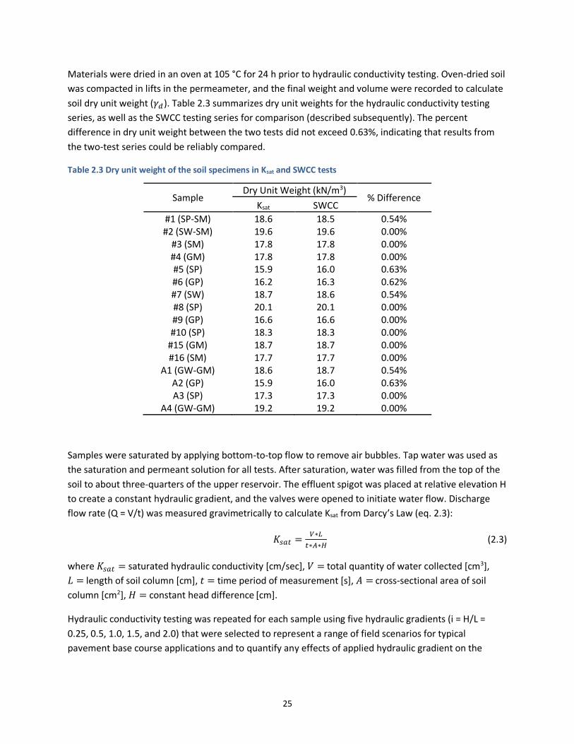
Materials were dried in an oven at 105 °C for 24 h prior to hydraulic conductivity testing. Oven-dried soil
was compacted in lifts in the permeameter, and the final weight and volume were recorded to calculate
soil dry unit weight (𝛾𝑑). Table 2.3 summarizes dry unit weights for the hydraulic conductivity testing
series, as well as the SWCC testing series for comparison (described subsequently). The percent
difference in dry unit weight between the two tests did not exceed 0.63%, indicating that results from
the two-test series could be reliably compared.
Table 2.3 Dry unit weight of the soil specimens in Ksat and SWCC tests
Sample Dry Unit Weight (kN/m3)
% Difference Ksat SWCC
#1 (SP-SM) 18.6 18.5 0.54% #2 (SW-SM) 19.6 19.6 0.00%
#3 (SM) 17.8 17.8 0.00% #4 (GM) 17.8 17.8 0.00% #5 (SP) 15.9 16.0 0.63% #6 (GP) 16.2 16.3 0.62% #7 (SW) 18.7 18.6 0.54% #8 (SP) 20.1 20.1 0.00% #9 (GP) 16.6 16.6 0.00% #10 (SP) 18.3 18.3 0.00%
#15 (GM) 18.7 18.7 0.00% #16 (SM) 17.7 17.7 0.00%
A1 (GW-GM) 18.6 18.7 0.54% A2 (GP) 15.9 16.0 0.63% A3 (SP) 17.3 17.3 0.00%
A4 (GW-GM) 19.2 19.2 0.00%
Samples were saturated by applying bottom-to-top flow to remove air bubbles. Tap water was used as
the saturation and permeant solution for all tests. After saturation, water was filled from the top of the
soil to about three-quarters of the upper reservoir. The effluent spigot was placed at relative elevation H
to create a constant hydraulic gradient, and the valves were opened to initiate water flow. Discharge
flow rate (Q = V/t) was measured gravimetrically to calculate Ksat from Darcy’s Law (eq. 2.3):
𝐾𝑠𝑎𝑡 =𝑉∗𝐿
𝑡∗𝐴∗𝐻 (2.3)
where 𝐾𝑠𝑎𝑡 = saturated hydraulic conductivity [cm/sec], 𝑉 = total quantity of water collected [cm3],
𝐿 = length of soil column [cm], 𝑡 = time period of measurement [s], 𝐴 = cross-sectional area of soil
column [cm2], 𝐻 = constant head difference [cm].
Hydraulic conductivity testing was repeated for each sample using five hydraulic gradients (i = H/L =
0.25, 0.5, 1.0, 1.5, and 2.0) that were selected to represent a range of field scenarios for typical
pavement base course applications and to quantify any effects of applied hydraulic gradient on the

26
measured hydraulic conductivity. Average Ksat values from test tests spanning the range of gradients
were calculated for subsequent modeling and analysis.
2.4 SOIL-WATER CHARACTERISTIC CURVE TESTING
Soil water characteristic curves (SWCCs) for the materials were measured using a hanging column test
apparatus (ASTM D6836). Figures 2.4(a) and (b) show a schematic and photograph of the testing
apparatus, respectively. The apparatus includes a large-diameter cell containing the compacted
specimen, a graduated outflow tube for measuring effluent water, and two reservoirs with a manometer
for applying suction pressure. Specimen diameter in the cell was 30.6 cm, while the specimen height
varied from 3.0 cm to 5.0 cm depending on grain size in order to maintain a representative grain size
distribution.
Samples for SWCC testing were compacted directly into the test cell to dry density values within 1% of
values used in the hydraulic conductivity tests (Table 2.3). The samples were saturated using tap water.
SWCCs were obtained along primary drying curves initiating at zero matric suction at full saturation to
matric suction of approximately 100 kPa. The highest applied suction corresponded to degree of
saturation ranging from near zero to 30%, depending on the material. Suction was applied in a series of
increments from 0.05 kPa to 100 kPa. The equilibrium position of the air-water interface in the
graduated outflow tube was measured to determine the volume of effluent for each increment and
calculate corresponding soil water content to produce the SWCC.
(a)

27
(b)
Figure 2.4 Large-scale hanging column apparatus: (a) schematic and (b) photograph

28
CHAPTER 3: EXPERIMENTAL RESULTS
3.1 HYDRAULIC CONDUCTIVITY
Figure 3.1 presents hydraulic conductivity results at each hydraulic gradient. Averages over the range of
gradient (Ksat,avg) are represented as dashed lines. Ksat values for the seven gravels and nine sandy soils
are tabulated in Table 3.1 and Table 3.2, respectively. Average Ksat for the gravels and the sandy soils
were 0.324 cm/sec and 0.014 cm/sec, respectively. While there was no significant effect of hydraulic
gradient on Ksat for the sandy soils (i.e., standard deviation was less than 1%), hydraulic gradient affected
Ksat measurements for the gravels (i.e., average standard deviation was 11.9%). Specifically, Ksat values
for the gravels decreased, except #15, with an increase in gradient from 0.25 to 2.0. This is potentially
due to effects of turbulent flow and/or migration and clogging of fines.
(a)
(b)
Figure 3.1 Hydraulic conductivity testing results for: (a) seven gravels and (b) nine sandy soils

29
Table 3.1 Hydraulic conductivity testing results for seven gravels
Sample Saturated Hydraulic Conductivity Ksat (cm/sec) Standard
Deviation Coefficient of
Variation i = 0.25 i =0.5 i = 1.0 i = 1.5 i = 2.0 Minimum Maximum Average
#4 (GM) 0.196 0.185 0.160 0.155 0.150 0.150 0.196 0.169 0.02 0.11
#6 (GP) 1.207 0.827 0.593 0.465 0.387 0.387 1.207 0.696 0.30 0.43
#9 (GP) 1.050 0.728 0.505 0.426 0.389 0.389 1.05 0.62 0.25 0.40
#15 (GM) 0.015 0.017 0.016 0.016 0.015 0.015 0.017 0.016 0.001 0.06
A1 (GW-GM) 0.034 0.032 0.030 0.028 0.025 0.025 0.034 0.03 0.003 0.10
A2 (GP) 0.874 0.612 0.493 0.434 0.396 0.396 0.874 0.562 0.17 0.31
A4 (GW-GM) 0.333 0.239 0.141 0.095 0.072 0.072 0.333 0.176 0.10 0.55
Table 3.2 Hydraulic conductivity testing results for nine sandy soils
Sample Saturated Hydraulic Conductivity Ksat (cm/sec) Standard
Deviation Coefficient of
Variation i = 0.25 i =0.5 i = 1.0 i = 1.5 i = 2.0 Minimum Maximum Average
#1 (SP-SM) 0.002 0.002 0.002 0.002 0.002 0.002 0.002 0.002 0 0.06
#2 (SW-SM) 0.003 0.003 0.003 0.003 0.003 0.003 0.003 0.003 0 0.06
#3 (SM) 0.007 0.008 0.007 0.007 0.007 0.007 0.008 0.007 0 0.04
#5 (SP) 0.050 0.048 0.048 0.049 0.050 0.048 0.05 0.049 0.001 0.01
#7 (SW) 0.021 0.023 0.024 0.025 0.025 0.021 0.025 0.024 0.002 0.08
#8 (SP) 0.005 0.005 0.005 0.005 0.005 0.005 0.005 0.005 0 0.04
#10 (SP) 0.015 0.017 0.016 0.016 0.015 0.015 0.017 0.016 0 0.02
#16 (SM) 0.0004 0.0004 0.0004 0.0005 0.0004 0.0004 0.0005 0.0004 0 0.05
A3 (SP) 0.030 0.025 0.019 0.019 0.019 0.019 0.030 0.022 0.005 0.20

30
3.2 SOIL-WATER CHARACTERISTIC CURVES
Figure 3.2 is a plot of soil-water characteristic curves (SWCCs) obtained from hanging column tests
(represented as symbols) and van Genuchten models (represented as solid lines). As summarized in
Table 3.3, fully saturated volumetric water contents (equivalent to porosity) varied from 0.23 m3/m3 to
0.39 m3/m3. As the applied suction pressure exceeded the air-entry pressure, the moisture content
began to decrease. Air-entry pressures for 16 samples were determined using a pair of two tangent lines
and ranged from 0.04 kPa (#4 GM) to 2.9 kPa (#2 SW-SM) with an average of 1.19 kPa (average of the
seven gravels = 0.61 kPa, average of the nine sands = 1.65 kPa). The matric suction gradually increased
with a decrease in the moisture. Then, the matric suction dramatically increased once the moisture
content reached a residual moisture content where the moisture is adsorbed on particle surfaces as thin
films due to short-ranged hydration mechanisms (Lu and Likos, 2004). Average residual water content
(r) for the seven gravels was 0.031, for the nine sands was 0.037, and the overall was 0.034. As
described in 1.4 Background (Lu and Likos, 2004), van Genuchten α parameter is inversely proportional
to the air-entry pressure and accordingly average van Genuchten α parameter for the seven gravels was
remarkably higher than the average for the nine sands (average α parameter for the seven gravels =
2.99, average α parameter for the nine sands = 0.45, the overall average = 1.56). Average van
Genuchten n parameter related to pore-size distribution for the seven gravels was 3.27, for the nine
sands was 2.72, and for the overall was 2.96.
(a)

31
(b)
(c)

32
(d)
Figure 3.2 Soil-water characteristic curves for: (a) gravels regarding volumetric water content, (b) gravels
regarding degree of saturation, (c) sandy soils regarding volumetric water content, and (d) sandy soils regarding
degree of saturation.
Table 3.3 Summary of SWCC parameters
Sample γd
(kN/m3) Air-Entry
Pressure (kPa)
van Genuchten (1980) SWCC Parameters
r s α n
#1 (SP-SM) 18.5 1.80 0.07 0.29 0.29 2.09
#2 (SW-SM) 19.6 2.90 0.07 0.24 0.20 3.16
#3 (SM) 17.8 0.59 0.00 0.32 0.77 1.23
#4 (GM) 17.8 0.04 0.00 0.32 13.26 1.17
#5 (SP) 16 0.45 0.03 0.38 1.07 2.31
#6 (GP) 16.3 0.46 0.03 0.37 1.57 6.48
#7 (SW) 18.6 1.70 0.04 0.28 0.38 3.45
#8 (SP) 20.1 0.80 0.00 0.23 0.57 2.24
#9 (GP) 16.6 0.30 0.03 0.36 1.93 3.97
#10 (SP) 18.3 2.10 0.04 0.30 0.29 4.62
#15 (GM) 18.7 2.10 0.00 0.28 0.20 1.20
#16 (SM) 17.7 2.60 0.08 0.32 0.16 1.65
A1 (GW-GM) 18.7 0.51 0.08 0.28 0.74 1.52
A2 (GP) 16 0.23 0.05 0.39 2.54 7.18
A3 (SP) 17.3 1.90 0.004 0.34 0.34 3.74
A4 (GW-GM) 19.2 0.60 0.03 0.26 0.65 1.40

33
CHAPTER 4: ANALYSIS
4.1 HYDRAULIC CONDUCTIVITY AND INDEX PROPERTIES
Index properties including D10, D30, D50, D60, % fines, % gravel, and Cu obtained from the particle-size
distribution curves were used along with as-compacted dry unit weights (γd) used during constant head
testing to evaluate relationships between these properties and measured Ksat values. Ksat for these
relationships is reported as Ksat,avg, representing an average of Ksat values under the five hydraulic
gradients. Table 4.1 summarizes Ksat,avg and the index properties for 16 samples.
Table 4.1 Index properties and dry unit weight (γd) of the soil specimens in permeameter
Sample Ksat,avg
(cm/sec) D10
(mm) D30
(mm) D50
(mm) D60
(mm) % Fines
% Retained Gravels
Cu γd
(kN/m3)
#1 (SP-SM) 0.002 0.09 0.30 0.46 0.55 8.8 0 5.9 18.6
#2 (SW-SM) 0.003 0.10 0.36 0.72 1.38 8.2 24.3 13.5 19.6
#3 (SM) 0.007 0.03 0.36 2.28 3.65 20.8 32.8 114.8 17.8
#4 (GM) 0.169 0.05 2.50 4.90 7.09 12.5 50.8 154.1 17.8
#5 (SP) 0.049 0.27 0.52 0.90 1.26 1.9 0.3 4.8 15.9
#6 (GP) 0.696 5.85 7.70 10.90 14.00 0.2 99.4 2.4 16.2
#7 (SW) 0.024 0.22 0.72 1.70 2.20 2 4.8 10.1 18.7
#8 (SP) 0.005 0.18 0.45 1.30 1.82 2.4 3.6 10.1 20.1
#9 (GP) 0.62 5.00 6.60 8.05 8.95 2.2 92.6 1.8 16.6
#10 (SP) 0.01 0.20 0.33 0.53 0.72 3.2 2.3 3.6 18.3
#15 (GM) 0.016 0.04 1.58 6.35 9.50 14.1 55.6 256.8 18.7
#16 (SM) 0.0004 0.02 0.13 0.44 0.79 23.4 0.1 46.9 17.7
A1 (GW-GM) 0.03 0.13 1.82 7.00 9.92 7.1 59 76.3 18.6
A2 (GP) 0.562 7.19 11.20 12.80 14.40 0.8 98.6 2 15.9
A3 (SP) 0.022 0.19 0.40 0.80 1.10 2.3 0.7 5.7 17.3
A4 (GW-GM) 0.176 0.08 0.93 5.20 7.99 9.9 51.9 102.4 19.2
Figure 4.1 plots relationships between Ksat,avg values and particle diameters corresponding to 10%, 30%,
50%, and 60% finer in each particle-size distribution curve. This includes a multivariable regression
(Figure 4.1d) on both D10 and D30. Even though there was a large gap of D10 data between the suite of
sandy soils and gravels, [Figure 4.1(a)] for D10 showed the most consistent single-variable regression
trend (i.e., the highest R-squared value). As the percent finer increased from D10 to D60, the gap in
particle diameters reduced with a decrease in the R-squared value. Generally, the relationships between
particle size and Ksat,avg showed similar trends. Ksat,avg increased with increases in the particle-size
parameters, due to general increases in pore sizes, particularly when the particle size was smaller than
4.75 mm. In other words, the presence of sands was more significant to Ksat,avg than gravels.

34
(a)
(b)

35
(c)
(d)

36
(e)
(f)
Figure 4.1 Relationships between experimentally obtained Ksat,avg values and (a) D10 in full range, (b) D10 in small
range except three outliers, (c) D30, (d) multivariable on D10 and D30, (e) D50, and (f) D60
Figure 4.2 is a series of relationships between Ksat and other index properties. In addition to the particle
size effects on Ksat,avg, % gravels, fines content, Cu, and dry unit weights correlated to Ksat,avg reflecting
pore structure changes. With a decrease in % gravels and increases in fines content and dry unit weight,

37
the pore space where liquid flow occurs can be expected to generally decrease, resulting in the decrease
in Ksat evident in the results. However, Ksat,avg only slightly decreased with an increase in Cu. That is, Cu
was not significantly correlated with Ksat,avg since samples including a significant percentage of small
particles can have both high and low Cu values depending on overall particle-size distribution.
(a)
(b)

38
(c)
(d)
Figure 4.2 Relationships between experimentally measured Ksat,avg and (a) %retained gravels, (b) % fines, (c) Cu,
and (d) γd
4.2 SOIL WATER CHARACTER ISTIC CURVES AND INDEX PROPERTIES
As described in the literature (e.g., Tinjum et al., 1997), shapes of the 16 SWCCs were dependent on the
particle-size distributions. For example, as shown in the experimentally obtained SWCCs (Figure 3.2),
matric suctions of #4, #15, A1, and A4 gravels, which had high Cu values (see Table 4.1), significantly

39
increased with a decrease in the moisture content (i.e., steep gradient of the SWCC slope), while only a
little matric suction increases (i.e., gentle slope) were required to remove the moisture in #6, #9, and A2
gravels, which had low Cu values. As well as the effect of Cu on the SWCC shape, the air-entry pressures
increased with an increase in Cu (Figure 4.3). These findings are interpreted to indicate that small
particles among the gravels (i.e., samples with high Cu) decreased the pore size, thus increasing air-entry
pressure and the matric suction at a given moisture content.
Figure 4.3 Relationship between air-entry pressure and uniformity coefficient
The van Genuchten (1980) fitting parameter α is inversely proportional to the air-entry pressure, and
van Genuchten fitting parameter n is related to pore size distribution (i.e., breadth of SWCC slope).
Figure 4.4 shows relationships between these two van Genuchten fitting parameters and air-entry
pressures obtained from the experimentally measured SWCCs (Table 3.3). In the analysis, #4 sample,
which had exceptionally higher α parameter (potentially due to experimental limitations), was excluded
to analyze the relationship in detail with a rescaled y-axis. Although R-squared values of the two
relationships were low, the trendlines were aligned well with the literature (e.g., Benson et al., 2014). As
the air-entry pressure increased, the parameters decreased.

40
(a) (b)
Figure 4.4 Relationships between air-entry pressure and van Genuchten parameters: (a) α and (b) n
4.3 FIELD CAPACITY, EFFECTIVE POROSITY AND MINIMUM SATURATION
Table 4.2 summarizes total porosity (n), field capacity (f), effective (drainable) porosity (nd), and
minimum saturation (Smin) for the 16 base materials used in this project. Field capacities were
determined using the SWCCs as volumetric moisture contents measured at 33 kPa (see background
section). Total porosity values were taken as saturated volumetric water contents (s) determined from
fitting the SWCCs with the van Genuchten (1980) model. Effective porosity and minimum saturation
were calculated using equations 1.15 and 1.16, respectively.
Tables A3 and A4 (Appendix A) represent typical effective porosities for a wider range of materials,
indicating a range from about 0.001 to 0.50 depending on soil type. Although the effective porosity for
#15 GM was exceptionally lower than other samples and the typical ranges, the 15 effective porosities
estimated here were generally in reasonable ranges. Minimum, maximum, and average effective
porosities for the 16 samples were 0.09 (#15 GM), 0.36 (#5 SP), and 0.24, respectively, and there was no
significant difference between averages for the seven gravels and the nine sands (average for the seven
gravels = 0.24, average for the nine sands = 0.23).

41
Table 4.2 Field capacities, effective porosities, and minimum saturations for 16 samples
Sample
Total Porosity
(n = s)
Field
Capacity (f) Effective
Porosity (nd) Minimum
Saturation (Smin)
#1 (SP-SM) 0.29 0.09 0.2 0.32
#2 (SW-SM) 0.24 0.08 0.17 0.31
#3 (SM) 0.32 0.15 0.16 0.48
#4 (GM) 0.32 0.11 0.2 0.35
#5 (SP) 0.38 0.03 0.36 0.08
#6 (GP) 0.37 0.03 0.35 0.07
#7 (SW) 0.28 0.03 0.25 0.10
#8 (SP) 0.23 0.002 0.22 0.01
#9 (GP) 0.36 0.02 0.34 0.06
#10 (SP) 0.3 0.04 0.26 0.14
#15 (GM) 0.28 0.19 0.09 0.69
#16 (SM) 0.32 0.17 0.15 0.53
A1 (GW-GM) 0.28 0.12 0.16 0.41
A2 (GP) 0.39 0.04 0.35 0.09
A3 (SP) 0.34 0.005 0.33 0.01
A4 (GW-GM) 0.26 0.10 0.17 0.36
Figure 4.5 presents a relationship between minimum saturation and % fines (%F) for the 16 samples. A
linear equation capturing this relation is in the form:
𝑆𝑚𝑖𝑛 = 0.025(%𝐹) + 0.062 (R2 = 0.75) (4.1)
As fines content increased, minimum saturation increased, due to potential decreases in pore sizes (i.e.,
increases in the matric suction), resulting in a decrease in the drainability of base materials. Similar
correlations between minimum saturation and index properties (D10, D30, D50, D60, Cu, % retained gravels)
were also explored, and these results are plotted in Appendix B. Minimum saturations decreased with
increases in D10, D30, and D50 and a decrease in Cu due to increases in pore spaces (i.e., a decrease in the
matric suction). Among the index properties, minimum saturations had relatively significant correlations
with D10 (R2 = 0.66) and Cu (R2 = 0.72). Overall, minimum saturations decreased (i.e., an increase in the
drainability) with decreases in % fines and Cu and an increase in D10.

42
Figure 4.5 Relationship between 16 minimum saturations and % fines
4.4 HYDRAULIC CONDUCTIVITY AND SWCC PARAMETERS
Experimentally measured Ksat,avg and van Genuchten parameters (α and n) of 15 samples (#4 was
excluded due to the exceptionally high α parameter) were compared to evaluate how the SWCC is
correlated to Ksat. The Ksat testing results and the two van Genuchten fitting parameters are summarized
in Table 4.3. Figure 4.6 presents relationships between the Ksat,avg and the two fitting parameters. When
the α and n parameters increased, Ksat increased. As described above, the high α and n parameters
indicate low air-entry pressure and SWCC breadth, respectively. Namely, Ksat increased with decreases in
the air-entry pressure and SWCC breadth (i.e., the decreased matric suction).

43
Table 4.3 Summary of Ksat,avg testing results and van Genuchten fitting parameters
Sample Ksat,avg
(cm/sec)
van Genuchten (1980) SWCC Parameters
r s α n
#1 (SP-SM) 0.002 0.07 0.29 0.29 2.09
#2 (SW-SM) 0.003 0.07 0.24 0.20 3.16
#3 (SM) 0.007 0.00 0.32 0.77 1.23
#4 (GM) 0.169 0.00 0.32 13.26 1.17
#5 (SP) 0.049 0.03 0.38 1.07 2.31
#6 (GP) 0.696 0.03 0.37 1.57 6.48
#7 (SW) 0.024 0.04 0.28 0.38 3.45
#8 (SP) 0.005 0.00 0.23 0.57 2.24
#9 (GP) 0.62 0.03 0.36 1.93 3.97
#10 (SP) 0.01 0.04 0.30 0.29 4.62
#15 (GM) 0.016 0.00 0.28 0.20 1.20
#16 (SM) 0.0004 0.08 0.32 0.16 1.65
A1 (GW-GM) 0.03 0.08 0.28 0.74 1.52
A2 (GP) 0.562 0.05 0.39 2.54 7.18
A3 (SP) 0.022 0.004 0.34 0.34 3.74
A4 (GW-GM) 0.176 0.03 0.26 0.65 1.40
(a) (b)
Figure 4.6 Relationships between van Genuchten parameters of Ksat,avg for 15 samples: (a) relationship between
van Genuchten parameter α and average Ksat,avg and (b) relationship between van Genuchten parameter n and
average Ksat,avg

44
4.5 HYDRAULIC CONDUCTIVITY FUNCTIONS
The unsaturated hydraulic conductivity function proposed by van Genuchten (1980) is one of the most
widely used equations in geotechnical engineering practice (Lu and Likos, 2004). The equation proposed
by van Genuchten (1980) describes a relationship between matric suction (ψ) and relative hydraulic
conductivity (Kr), which is defined as a ratio of unsaturated (KU) to saturated hydraulic conductivity (Ksat),
as described in 1.4.7 Hydraulic Conductivity Function Modeling chapter. Unsaturated hydraulic
conductivity functions for the 16 samples were calculated using eq. (1.13) and the experimentally
obtained data for Ksat and van Genuchten fitting parameters.
Figure 4.7 summarizes hydraulic conductivities as a function of the matric potential for the 16 samples.
Hydraulic conductivities of the samples that have a relatively high n fitting parameter were significantly
decreased (e.g., n parameter for #6 GP = 6.48, n parameter for #9 GP = 3.97, n parameter for #10 SP =
4.62, n parameter for A2 GP = 7.18) as the high n parameter indicates a narrow distribution of pore sizes
(Benson et al., 2014).
(a)

45
(b)
Figure 4.7 Hydraulic conductivity functions using van Genuchten (1980) approach: (a) unsaturated hydraulic
conductivity functions for six gravels, and (b) unsaturated hydraulic conductivity functions for nine sandy soils.
4.6 SATURATED HYDRAULIC CONDUCTIVITY MODELS
4.6.1 Models from the Literature
As summarized in Appendix C, there are a large number of empirical equations that may be used to
estimate Ksat. Most of the equations are based on soil physical properties, particularly particle-size
distributions (e.g., D10) that can be readily obtained by the sieve test.
13 applicable model equations were selected among the empirical equations described in Appendix C to
estimate Ksat values for the 16 samples. The selected empirical equations were primarily based on soil
porosity and index properties directly obtained from a particle-size distribution curve. The equations
used in this study were as follows: Alyamani and Sen (Equation C.21), Beyer (Equation C.12), Harleman
et al. (Equation C.11), original Hazen (Equation C.1a), modified Hazen (Equation C.1b), Kozeny (Equation
C.9), Kozeny-Carman (Equation C.10), Sauerbrei (Equation C.19), Slichter (Equation C.3), Terzaghi
(Equation C.5), U.S. Bureau of Reclamation (Equation C.20), Salarashayeri and Siosemarde (Equation
C.25), and Chapuis (Equation C.28).
Table 4.4 summarizes measured and estimated Ksat values for the 16 samples. Ksat values estimated for
#6, #9 and A2 gravels (poorly graded gravels, GP), only except two Ksat values estimated using Original

46
Hazen (C.1a) and Salarashayeri and Siosemarde (Equation C.25), were significantly higher than the
experimentally measured Ksat values. The three GPs had higher D10 values (D10 for #6 = 5.85 mm, D10 for
#9 = 5.00 mm, D10 for A2 = 7.19 mm) than other gravels (D10 values were less than 2.5 mm), and the high
D10 values caused the overestimations. Except the three GPs, the Ksat estimations were in reasonable
ranges showing low standard deviations (less than 3%).
Averages of Ksat values estimated using the empirical equations for each sample (i.e., Avg. row in Table
4.4) were compared to averages of the experimentally measured Ksat values under the five hydraulic
gradients (Figure 4.8). The solid line in the figure denotes 1:1 correspondence and the dashed lines
denote correspondence plus or minus 10%. The three GPs, #6, #9, and A2, were excluded in the analysis.
Ksat values for #4 and A4 gravels (GM and GW-GM, respectively) were significantly underestimated, as
highlighted in red [Figure 4.8(a)]. This suggests that the empirical equations considered may not be
applicable for estimating Ksat of gravels as estimation results for the five gravels out of total seven gravel
samples (#4, #6, #9, A2, A4) were exceptionally out of range. The two gravels, as well as the three GPs,
were excluded and the axes were rescaled in Figure 4.8(b) to compare the results in detail. Although #15
and A1 gravels (GM and GW-GM, respectively) were still underestimated as highlighted in red [Figure
4.8(b)], the estimations for #15 and A1 were in reasonable ranges compared to the estimations for other
five gravels as described above.
In addition to the comparisons of average Ksat values obtained from experiments and estimations, Ksat
values estimated using each of the empirical equations for the 11 samples that excluded the five outliers
(i.e., #4, #6, #9, A2, and A4 gravels) were individually compared to averages of experimentally measured
ksat values obtained under the five hydraulic gradients (Figure 4.9). The Ksat values were underestimated
when Ksat values were estimated using original Hazen (1892), Kozeny (1953), Kozeny-Carman (Kozeny,
1953; Carman, 1956), Slichter (1899), Terzaghi (1925), and U.S. Bureau of Reclamation, while the Ksat
values were overestimated when they were estimated using Alyamani and Sen (1993). Furthermore,
when Ksat values were estimated using Alyamani and Sen (1993), Beyer (1964), modified Hazen (1892),
Salarashayeri and Siosemarde (2012), the estimated ksat values were scattered. Overall, the Ksat
estimations were relatively well aligned with the experimentally measured Ksat values for aggregate base
and sand when Ksat values were estimated using Chapuis (2004), Harleman et al. (1963), and Sauerbrei
(1932).

47
Table 4.4 Summary of saturated hydraulic conductivity estimated using 13 applicable empirical equations
Method Saturated Hydraulic Conductivity (cm/sec)
#1 #2 #3 #4 #5 #6 #7 #8 #9 #10 #15 #16 A1 A2 A3 A4
M1 0.008 0.009 0.007 0.028 0.063 39.539 0.046 0.033 31.235 0.047 0.042 0.0004 0.071 60.103 0.038 0.037
M2 0.010 0.010 0.000 0.001 0.083 46.499 0.047 0.032 35.815 0.050 0.000 0.0002 0.008 72.582 0.042 0.002
M3 0.006 0.004 0.001 0.003 0.075 8.565 0.021 0.008 5.972 0.021 0.001 0.0005 0.009 12.985 0.029 0.003
M4 0.006 0.007 0.001 0.001 0.045 21.833 0.030 0.021 15.949 0.026 0.001 0.0002 0.011 32.981 0.024 0.004
M5 0.007 0.006 0.001 0.002 0.001 0.442 0.000 0.000 0.304 0.000 0.000 0.0000 0.000 0.701 0.000 0.000
M6 0.009 0.010 0.001 0.002 0.070 34.223 0.048 0.032 25.000 0.040 0.001 0.0003 0.017 51.696 0.037 0.006
M7 0.000 0.000 0.000 0.000 0.009 3.985 0.002 0.001 2.514 0.002 0.000 0.0000 0.001 6.782 0.003 0.000
M8 0.002 0.002 0.000 0.001 0.062 26.658 0.012 0.004 16.817 0.012 0.000 0.0001 0.004 45.370 0.018 0.001
M9 0.013 0.004 - - 0.024 0.538 - 0.002 0.505 0.025 - 0.0009 - 0.691 0.017 -
M10 0.008 0.005 0.001 0.030 0.069 22.092 0.020 0.005 14.761 0.015 0.003 0.0004 0.008 47.376 0.024 0.003
M11 0.001 0.001 0.000 0.000 0.032 13.960 0.008 0.003 9.091 0.008 0.000 0.0001 0.003 23.122 0.010 0.001
M12 0.002 0.001 0.000 0.001 0.040 17.614 0.009 0.002 11.399 0.009 0.000 0.0001 0.003 29.295 0.013 0.001
M13 0.002 0.003 0.000 0.045 0.007 4.930 0.008 0.003 3.524 0.003 0.001 0.0001 0.002 10.459 0.003 0.001
Avg. 0.006 0.005 0.001 0.008 0.047 17.499 0.021 0.012 12.613 0.021 0.004 0.0003 0.011 28.449 0.021 0.005
STDV 0.003 0.003 0.002 0.014 0.026 13.763 0.016 0.012 10.526 0.015 0.011 0.0002 0.017 21.717 0.013 0.009
Ksat,test 0.002 0.003 0.007 0.169 0.049 0.696 0.024 0.005 0.620 0.010 0.016 0.0004 0.030 0.562 0.022 0.176
% Diff. 93% 55% 148% 181% 5% 185% 10% 80% 181% 66% 123% 47% 93% 192% 8% 190%
Closest to Ksat
M13 M13 M1 M13 M4 M9 M3 M10 M9 M12 M10 M10 M6 M9 M4 M1
Note: M1 = Alyamani and Sen (1993), M2 = Beyer (1964), M3 = Chapuis et al. (2005), M4 = Harleman et al. (1963), M5 = Hazen-Original (1892), M6 = Hazen-Modified, M7 = Kozeny (1953), M8 = Kozeny-Carman (Kozeny 1927, 1953; Carman1937, 1956), M9 = Salarashayeri and Siosemarde (2012), M10 = Sauerbrei (1932), M11 = Slichter (1899), M12 = Terzaghi (1925), M13 = U.S. Bureau of Reclamation, STDV = Standard deviation, Ksat,test = Saturated hydraulic conductivity obtained from constant head tests, % Diff. = percentage difference between average of estimations obtained using 13 equations and average of measurements under five hydraulic gradients, Closest to Ksat = model which is the closest to experimentally obtained Ksat for each sample.

48
(a) (b)
Figure 4.8 Comparisons of experimentally measured and estimated Ksat values for (a) 13 samples and (b) 11
samples
(a) (b)

49
(c) (d)
(e) (f)

50
(g) (h)
(i) (j)

51
(k) (l)
(m)
Figure 4.9 Comparisons of estimated and measured Ksat for 11 samples excluding #4, #6, #9, A2, and A4 using (a)
Alyamani and Sen (1993), (b) Beyer (1964), (c) Chapuis et al. (2005), (d) Harleman et al. (1963), (e) Hazen-Original
(1892), (f) Hazen-Modified, (g) Kozeny (1953), (h) Kozeny-Carman (Kozeny 1927, 1953; Carman1937, 1956), (i)
Salarashayeri and Siosemarde (2012), (j) Sauerbrei (1932), (k) Slichter (1899), (l) Terzaghi (1925), and (m) U.S.
Bureau of Reclamation

52
4.6.2 Dataset Specific Models
As most Ksat values estimated using the 13 existing empirical equations for gravels did not reveal ideal
correspondence, regression equations shown with trendlines in Figure 4.1 from the specific dataset
considered here were used to estimate Ksat values for the 16 samples. The equations developed from
Figure 4.1 are as follows:
𝐾𝑠𝑎𝑡 = 0.0956 × 𝐷10 + 0.0322 (R2 = 0.89) (4.2)
𝐾𝑠𝑎𝑡 = 0.0684 × 𝐷30 − 0.004 (R2 = 0.85) (4.3)
𝐾𝑠𝑎𝑡 = 0.0286 + 0.0878 × 𝐷10 + 0.0058 × 𝐷30 (R2 = 0.89) (4.4)
𝐾𝑠𝑎𝑡 = 0.0032 × 𝐷502 + 0.0144 × 𝐷50 − 0.008 (R2 = 0.74) (4.5)
𝐾𝑠𝑎𝑡 = 0.0386 × 𝐷60 − 0.0566 (R2 = 0.60) (4.6)
where, 𝐾𝑠𝑎𝑡 = saturated hydraulic conductivity [cm/sec], 𝐷10, 𝐷30, 𝐷50, 𝐷60 = particle sizes
corresponding to 10%, 30%, 50%, 60% finer, respectively, in particle-size distribution curve [mm].
Figure 4.10 compares the estimated Ksat values from these equations and the experimentally measured
Ksat values. Outliers above the 10% lines are highlighted in red. While Ksat values estimated using the
existing empirical equations obtained from the literature showed unrealistic overestimations for the
three GPs (#6, #9, and A2) as described in Table 4.4, Ksat values estimated using the five dataset specific
regression equations demonstrated reasonable estimation results for the three samples, particularly
when they were estimated using the equation based on D10, D30, and the multivariable regression on D10
and D30 (i.e., the closest to the one-to-one line). However, #9 GP was greatly underestimated when
using the regression equations based on D50 and D60, and A2 GP.
(a) (b)
D10-Based Equation D30-Based Equation

53
(c) (d)
(e)
Figure 4.10 Comparisons of Ksat values obtained from experiments and estimations using regression equations
based on (a) D10, (b) D30, (c) multivariable on D10 and D30, (d) D50, and (e) D60
In addition to the improved Ksat estimations for the three GPs, the estimation results for #4 and A4
gravels, which were considerably underestimated with the existing model equations from the literature
[Figure 4.8(a)], were improved with the regression equations based on D30, D50, and D60. In contrast, the
equations based on D10 still underestimated Ksat values for #4 and A4 gravels, as well as #6 and #9
gravels, while other soils were slightly overestimated. As described in Appendix C, most of the existing
empirical equations were derived based on D10 (or less than D30). That is, Ksat values for #4 and A4
gravels were underestimated when the Ksat estimation equations were derived based on D10 (or less than
D30). These results suggest that pore structures of #4 and A4 gravels were not represented and governed
D10 & D30-Based Equation D50-Based Equation
D60-Based Equation

54
by the particle diameter corresponding to 10% and 30% finer in entire particle-size distributions of the
two gravels.
Although the dataset specific Ksat estimations improved the estimation results for #4 and A4 gravels, at
the same time, results were overestimated for #15 and A1 gravels. Moreover, the overall estimations
using the two equations based on D50, and D60 were scattered due to low R-squared values: 1) R-squared
value for relationship between Ksat and D10 = 89.4%, 2) R-squared value for relationship between Ksat and
D30 = 85.3%, 3) R-squared value for relationship between Ksat and multivariable on D10 and D30 = 89.4%,
4) R-squared value for relationship between Ksat and D50 = 74.0%, and 5) R-squared value for relationship
between Ksat and D60 = 60.1%. Consequently, among the regression equations, the equations based on
D10 and D30, particularly D10 that is one of the most broadly used parameters in the literature to estimate
Ksat, provided reasonable estimation results for gravels (i.e., aggregate base). The equation based on D30
provided generally reasonable estimation results and the equation based on D10 showed the best
estimation performance for large-sized gravels.
4.6.3 Performance Evaluation and Improvement of D1 0-Based Equation using Data from
the Literature
In this section, performance of eq. (4.2), which showed the most reliable estimation results (i.e., the
closest to the one-to-one line), was evaluated using Ksat and D10 data for a wider range of experimental
data. This included various recycled base materials obtained from the literature (Trzebiatowski and
Benson 2015, Cetin et al., 2021, Klink, 2021). In these three studies, laboratory tests were conducted to
measure Ksat values of recycled asphalt pavement (RAP) and recycled concrete aggregate (RCA) materials
widely used in pavement systems. Table 4.5 summarizes Ksat and D10 data obtained from the literature.
Figure 4.11 compares the experimentally measured Ksat and Ksat estimated using eq. (4.2) for the 16
samples used in this study and including the recycled base materials obtained from the literature. In the
full scale [Figure 4.11(a)], even though Ksat estimations for the recycled base materials were located
above the one-to-one line (i.e., overestimations), the estimation results were in reasonable ranges (e.g.,
inside the 10% lines). On the other hand, in the small scale [Figure 4.11(b)] excluding the three GPs,
most of estimation results particularly for the recycled base materials were located above 10% line. The
16 samples and recycled base materials had similar D10 values, but Ksat values of the recycled base
materials were generally lower than those of the 16 samples potentially due to different compaction
efforts and particle-size distributions (e.g., different % retained gravels). This difference in Ksat
measurements correspondingly results in the overestimations notwithstanding similar D10.

55
Table 4.5 Experimentally measured Ksat and D10 data of recycled base materials obtained from the literature
Source Sample D10 (mm) Ksat (cm/s) Note
Trzebiatowski and Benson
2015
PDF RAP 0.316 0.009 Compacted with standard Proctor
effort in compaction-mold permeameter
PDV RAP 0.4 0.0038
WSP RAP 0.16 0.0024
Lodi Gravel 0.089 0.000058
Cetin et al. 2021
Coarse RCA 0.37 0.000488
Compacted using light hammering
method (degree of compaction of 95%)
Fine RCA 0.135 0.00099
Limestone 0.038 0.000191
RCA+RAP 0.1 0.000479
Class 6 Aggregate
0.175 0.000491
Class 5Q Aggregate
0.4 0.000733
Sand Subgrade 0.048 0.000715
Klink (2021)
RCA DC-10 0.14 0.000412
Hand tampered in flexible wall
permeameter
RCA DC-1 0.20 0.000731
RCA DC-7 0.13 0.000111
RCA MC-1 0.25 0.001422
RCA DC-6 0.16 0.00036
RCA DC-8 0.56 0.005822
RCA RC-1 0.24 0.000502
RCA RC-2 0.23 0.002492
RAP DRAP-1 0.72 0.128839
RAP DRAP-2 0.61 0.117

56
(a) (b)
Figure 4.11 Comparisons of Ksat measurements and estimations obtained using eq. (4.2) for base materials: (a) in
full range and (b) in small range excluding #6, #9, and A2
To improve the estimation performance, eq. (4.2) was incorporated with Ksat and D10 data of the
recycled base materials. As mentioned above, most of the recycled base materials had similar D10 values
between 0 mm and 1 mm and lower Ksat values (Figure 4.12). With the additional data set of recycled
base materials, overall trend was same showing a slight change in the equation (eq. 4.7).
Figure 4.12 Relationship between Ksat and D10 of 16 samples and recycled base materials

57
𝐾𝑠𝑎𝑡 = 0.0999 × 𝐷10 + 0.0043 (R2 = 0.89) (4.7)
where, 𝐾𝑠𝑎𝑡 = saturated hydraulic conductivity [cm/sec], 𝐷10 = particle diameter corresponding to 10%
finer on the cumulative particle-size distribution curve [mm]. Ksat values for the 16 samples and recycled
base materials obtained from experiments and estimated using eq. (4.7) were compared in Figure 4.13.
Despite Ksat estimations for the #4 and A4 gravels were even lower when using eq. (4.7), overall
estimations for the recycled base materials were moved to the one-to-one line. Future, additional tests
are recommended to collect more Ksat data for the medium-sized gravels that have D10 between 2 mm
and 8 mm and accordingly improve reliabilities of the equation.
(a) (b)
Figure 4.13 Comparisons of Ksat measurements and estimations obtained using eq. (4.7) for base materials: (a) in
full range and (b) in small range excluding #6, #9, and A2
4.7 SOIL-WATER CHARACTERISTIC CURVE MODELS
4.7.1 Benson et al (2014)
Benson et al. (2014) performed hanging column tests (ASTM D6836) to measure SWCCs of sands having
a wide range of D50 and Cu and proposed pedotransfer functions (PTF) to estimate the van Genuchten
parameters α and n. For fitting parameters corresponding to drying SWCCs (i.e., those measured here).
Equations to estimate were proposed as:

58
𝛼 = 𝛼1𝑁𝛼 (4.8a)
where, 1 = derived from regression with grain size parameter D60, N = a normalized value derived
from regression with Cu. For the clean and uniform sands in Benson et al (2014):
𝛼1 = 1.354𝐷60 (4.8b)
𝑁𝛼 = 0.99𝐶𝑢−0.54 (4.8c)
Equations to estimate n were proposed as:
𝑛 = 𝑛1𝑁𝑛 (4.9a)
where, n1 = derived from regression with grain size parameter D60, Nn = a normalized n value derived
from regression with Cu. For the clean and uniform sands in Benson et al (2014):
𝑛1 = 14.4 exp(−0.434𝐷60) (4.9b)
𝑁𝑛,𝐶𝑢<2.2 = −0.542𝐶𝑢 + 1.542 (4.9c)
𝑁𝑛,𝐶𝑢≥2.2 = −0.0033𝐶𝑢 + 0.379 (4.9d)
Equations for estimating van Genuchten parameters were rederived using the procedures described in
Benson et al. (2014) with the experimental results for the 15 base aggregates and sands in this study.
Procedures for deriving the equations were as follows:
1) Experimentally obtained D60 and van Genuchten parameters α and n were plotted to derive
regression equations. Sample #4 was excluded due to the exceptionally high α.
2) Uniformity coefficients Cu were plotted with normalized van Genuchten parameters. Normalized
parameters are defined as ratios of the or n parameter for a given Cu to the or n parameter
for a nominally uniformly graded soil. In this study, Sample #9 (GP), which has the lowest Cu
value (Cu = 1.79), was used as the uniformly graded sample for normalizing the parameters.
Figure 4.14(a) and Figure 4.14(b) show relations between the α and n parameters and D60 and
corresponding regression equations. Figure 4.14(c) and Figure 4.14(d) show relations between the
normalized α and n parameters and Cu.

59
(a) (b)
(c) (d)
Figure 4.14 Deriving new regression equations using experimental results of 15 samples: (a) relationship
between D60 and van Genuchten parameter α, (b) relationship between D60 and van Genuchten parameter n, (c)
relationship between Cu and normalized α, and (d) relationship between Cu and normalized n
Resulting equations to estimate based on the materials in this study are:
𝛼 = 𝛼1𝑁𝛼 (4.10)
where

60
𝛼1 = 0.0104 × 𝐷602 − 0.0408 × 𝐷60 + 0.4617 (R2 = 0.59)
𝑁𝛼 = −0.12 ln(𝐶𝑢) + 0.7155 (R2 = 0.28)
Resulting equations to estimate n based on the materials in this study are:
𝑛 = 𝑛1𝑁𝑛 (4.11)
where
𝑛1 = 0.0763 × 𝐷602 − 0.88 × 𝐷60 + 3.7878 (R2 = 0.70)
𝑁𝑛 = 1.5107 × 𝐶𝑢−0.3187
(R2 = 0.79)
Figure 4.15 compares 15 sets of the van Genuchten parameters estimated using the new equations
(equations 4.10 and 4.11). As highlighted in Figure 4.14(a), some D60 values were not robustly correlated
with the experimentally obtained α, and these led to significant underestimations for α parameters of
#3, #5, #9, and A2, as well as general underestimations for other samples [Figure 4.15(a)]. In other
words, the air-entry pressure related to the α parameter may not be correlated well with D60. On the
other hand, even though n parameters for some samples were underestimated below the 10% line, the
estimated n parameters were generally well aligned with the experimentally obtained n parameters
[Figure 4.15(b)]. Namely, breadth of SWCC slope (related to the n parameter) was well represented with
D60.
(a) (b)
Figure 4.15 Comparisons of van Genuchten parameters obtained from experiments and estimations: (a)
comparison of α parameters, (b) comparison of n parameters.

61
4.7.2 Dataset Specific Models
Additional regression equations were derived with D10, D30, D50 and dry unit weight (γd) data for the 15
samples. To derive the equations, experimentally obtained van Genuchten parameters and the index
properties were plotted with trendlines (Figure 4.16). Figure 4.16 demonstrates that both α and n
parameters increased as the particle size (i.e., D10, D30, D50) increased and γd decreased. That is, the
increased pore sizes (caused by increases in D10, D30, and D50 and a decrease in γd) resulted in decreases
in the air-entry pressure and the gradient of SWCC (i.e., increases in α and n parameters).
(a) (b)
(c) (d)

62
(e) (f)
(g) (h)
Figure 4.16 Relationships between experimentally obtained van Genuchten fitting parameters and index
properties: (a) relationship between α and D10, (b) relationship between n and D10, (c) relationship between α
and D30, (d) relationship between n and D30, (e) relationship between α and D50, (f) relationship between n and
D50, (g) relationship between α and γd, and (h) relationship between n and γd

63
The regression equations for estimating α are as follows:
𝛼 = 0.0094 × 𝐷102 + 0.2039 × 𝐷10 + 0.4443 (R2 = 0.85) (4.12)
𝛼 = 0.0008 × 𝐷302 + 0.1843 × 𝐷30 + 0.3567 (R2 = 0.85) (4.13)
𝛼 = 0.0147 × 𝐷502 − 0.0309 × 𝐷50 + 0.4361 (R2 = 0.74) (4.14)
𝛼 = 0.1926 × 𝛾𝑑2 − 7.2573 × 𝛾𝑑 + 68.6876 (R2 = 0.68) (4.15)
The regression equations for estimating n are as follows:
𝑛 = 0.0723 × 𝐷102 + 0.1570 × 𝐷10 + 2.3413 (R2 = 0.69) (4.16)
𝑛 = 0.0419 × 𝐷302 + 0.0073 × 𝐷30 + 2.4052 (R2 = 0.65) (4.17)
𝑛 = 0.09 × 𝐷502 − 0.793 × 𝐷50 + 3.3674 (R2 = 0.73) (4.18)
𝑛 = 0.3442 × 𝛾𝑑2 − 13.087 × 𝛾𝑑 + 126.53 (R2 = 0.40) (4.19)
where, D10, D30, and D50 = particle diameters in mm corresponding to 10%, 30%, and 50% finer in the
particle-size distribution curve, respectively, γd = dry density in kN/m3. Using the equations above and
the 15-sample data, van Genuchten parameters were estimated. Similar to Figure 4.15(a), almost all
estimation results for α parameters were located below the one-to-one line (i.e., underestimation),
while estimation results for n parameters were in reasonable ranges. Among the n parameter
estimation results, the equations based on D30 showed the best performance (i.e., the estimated van
Genuchten parameters were the closest to the one-to-one line), and these results are interpreted to
reflect the highest R-squared values. That is, the performance improvements are expected with adding
robust data set that can increase the R-squared values.

64
(a) (b)
(c) (d)
D30-Based Equation D30-Based Equation
D10-Based Equation D10-Based Equation

65
(e) (f)
(g) (h)
Figure 4.17 Comparisons of van Genuchten parameters obtained from experiments and pedotransfer functions
based on: (a) D10 for α parameter, (b) D10 for n parameter, (c) D30 for α parameter, (d) D30 for n parameter, (e)
D50 for α parameter, (f) D50 for n parameter, (g) γd for α parameter, and (h) γd for n parameter
D50-Based Equation D50-Based Equation
γd-Based Equation γd-Based Equation

66
CHAPTER 5: CONCLUSIONS AND RECOMMENDATIONS
5.1.1 Summary and Key Findings
The objective of this project is to assess the drainability of coarse soil/aggregate materials applicable to
pavement base course applications. Emphasis is placed on saturated hydraulic conductivity and water
retention curves, including evaluation of existing predictive equations for indirect estimation of these
properties from surrogate material properties (e.g., grain size distribution) and the development of new
correlation equations from the materials examined here. Samples of 16 representative materials were
obtained from NRRA stakeholders, including materials that are generally classified as gravels (7 samples)
and sands (9 samples).
Laboratory tests were conducted to determine grain size distribution, grain size index properties,
saturated hydraulic conductivity (Ksat), and soil-water characteristic curves (SWCCs). Key findings from
the experimental program included the following:
1) Measured Ksat of the sandy materials was independent of applied hydraulic gradient (i) typical of
field conditions for pavement base applications (0.25 < i < 2.0). Measured Ksat of the gravels
systematically decreased with increasing hydraulic gradient, potentially due to migration of fines
and the effects of turbulent flow. Average Ksat values over the range of applied gradient was
calculated for subsequent analysis.
2) Ksat for all materials generally increased as % gravels and particle diameters corresponding to
10%, 30%, 50%, and 60% finer (D10, D30, D50, and D60, respectively) increased. Ksat generally
increased as % fines and dry unit weight (γd) decreased.
3) Ksat slightly increased with a decrease in uniformity coefficient (Cu), but the relationship was not
significantly correlated. Air-entry pressure on measured soil-water characteristic curves
increased with an increase in Cu.
4) The van Genuchten (1980) SWCC parameters (α and n) increased with increases in D10, D30, D50,
D60, and % retained gravels and with decreases in % fines, Cu, and γd. Comparisons among the
experimentally measured Ksat values and the van Genuchten α and n parameters showed a
proportional relationship.
5) Effective (drainable) porosities for the 16 samples ranged from 0.26 (#15 GM) to 0.59 (#5 SP)
with an average of 0.42 and were comparable to typical values obtained from the literature.
Test results were analyzed to examine the accuracy and applicability of equations available in the
literature for estimating Ksat and SWCC parameters for coarse materials and to develop dataset-specific
equations for the suite of materials tested here. This analysis showed:
1) Estimated Ksat for materials that classified as poorly graded gravel (GP) were significantly higher
than the experimentally measured Ksat values. Measured Ksat values for a subset of samples that
excluded the gravels were generally well estimated using the Harleman et al. (1963), Sauerbrei
(1932), and Chapuis (2004) empirical equations.
2) New dataset-specific regression equations to estimate Ksat were derived using the
experimentally obtained Ksat and index properties (D10, D30, D50, D60). Measured Ksat values that

67
were overestimated using the existing equations were reasonably estimated with the new
equations, particularly using single-variable equations based on D10 and D30.
3) The van Genuchten (1980) SWCC fitting parameters α and n were estimated using regression
equations obtained by following procedures developed by Benson et al. (2014). New dataset-
specific equations were derived using the Benson et al., (2014) approach. Equations based on
D30 and Cu showed the best performance.
5.1.2 Qualitative Material Rating System for Base Course Drainability
As noted in Section 1.4.8, the drainability of pavement systems in the field depends on several factors:
1) Base course permeability, including both saturated hydraulic conductivity and the unsaturated
hydraulic conductivity function.
2) Effective (drainable) porosity (ratio of the volume of the voids that can be drained under gravity
flow to the total volume of material.) Corresponding minimum saturation is the minimum
saturation that is achieved by gravity and can be estimated from the field capacity
corresponding to a suction value of 33 kPa.
3) Drainage boundary conditions, including the cross-sectional geometry of the pavement system,
depth to the water table, side-slope geometry, and any installed drainage systems.
4) Environmental conditions, including surface water, groundwater, temperature, wind speed, and
relative humidity. The volume of infiltration into the pavement system will depend on factors
such as type and condition of surface, length and intensity of rainfall, properties of the drainage
layer, hydraulic gradient, time allowed for drainage and the drained area.
Rigorous drainability analysis, therefore, requires knowledge of material properties, pavement system
design, and site environmental conditions, thereby allowing site-specific time-to-drainage analyses to be
conducted. In lieu of knowledge of system design parameters and site environmental conditions,
however, base course material properties may be used to screen candidate materials for drainability
performance. If saturated hydraulic conductivity (Ksat) and minimum saturation (Smin) are adopted as
screening parameters for base course material performance, criteria must be selected to quantify
acceptable ranges for these properties.
Table 5.1 summarizes recommended bounds for Ksat and Smin to meet qualitative drainability
assessments of “excellent,” “marginal,” and “poor.” The criteria for Ksat are based on Federal Highway
Administration (FHWA) guidance describing drainability for an excellent-quality material equivalent to
0.353 cm/sec (1,000 ft/day) (FHWA, 1992), while a base layer that has a coefficient of permeability (Ksat)
of less than 0.017 cm/sec (48 ft/day) is practically impermeable (McEnroe, 1994). Criteria for Smin are
based on characteristics of material that may be considered “freely draining” under gravity (McEnroe,
1994).

68
Table 5.1 Recommended material parameters for qualitative drainability assessment of pavement base course
materials
Qualitative Drainability
Hydraulic Conductivity
(cm/s)
Minimum Saturation
Excellent Ksat ≥ 0.35 Smin ≤ 0.10
Marginal 0.02 ≤ Ksat < 0.35 0.10 < Smin ≤ 0.30
Poor Ksat < 0.02 Smin > 0.30
Approaches for either direct measurement of Ksat and Smin (e.g., permeability and SWCC testing) or their
indirect estimation (e.g., based on grain size indices) must be adopted to apply the qualitative rating
system. Three recommendations for such approaches are summarized below.
5.1.3 Recommendation 1: Qualitative Material Rating Based on Direct Measurements of
Permeability and Water Retention
Table 5.2 summarizes ratings for each material examined in this study based on direct measurements of
Ksat and Smin. The experimentally obtained Ksat values for the 16 base aggregates and sands ranged from
0.0004 cm/sec (#16, SM) to 0.6957 cm/sec (#6, GP). The three GPs (#6, #9, and A2) satisfied the Ksat
criterion for “excellent” quality, five materials are designated “marginal,” and 8 materials are designated
as “poor.” Another 7 of the materials classify as “excellent” with respect to minimum water retention,
four as “marginal,” and five as “poor.” The overall ratings reflect the combination of the permeability
and water retention criteria.

69
Table 5.2 Qualitative performance rating of materials based on measured permeability and water retention
Sample Ksat
(cm/s) Minimum Saturation
Ksat Criterion Smin Criterion Overall Rating
#1 (SP-SM) 0.0021 0.32 Poor Marginal Poor-Marginal
#2 (SW-SM) 0.0027 0.31 Poor Marginal Poor-Marginal
#3 (SM) 0.0073 0.48 Poor Poor Poor
#4 (GM) 0.1693 0.35 Marginal Poor Marginal
#5 (SP) 0.0489 0.08 Marginal Excellent Marg - Excellent
#6 (GP) 0.6957 0.07 Excellent Excellent Excellent
#7 (SW) 0.0236 0.10 Marginal Excellent Marginal
#8 (SP) 0.0050 0.01 Poor Excellent Marginal
#9 (GP) 0.6196 0.06 Excellent Excellent Excellent
#10 (SP) 0.0104 0.14 Poor Marginal Poor-Marginal
#15 (GM) 0.0159 0.69 Poor Poor Poor
#16 (SM) 0.0004 0.53 Poor Poor Poor
A1 (GW-GM) 0.0298 0.41 Marginal Poor Poor-Marginal
A2 (GP) 0.5618 0.09 Excellent Excellent Excellent
A3 (SP) 0.0224 0.01 Marginal Excellent Marg - Excellent
A4 (GW-GM) 0.1759 0.36 Poor Marginal Poor-Marginal
5.1.4 Recommendation 2: Qualitative Material Rating Based on Grain Size Indices
If Ksat and the SWCC are not directly measured, then the empirical relations developed in this study can
be used to indirectly estimate Ksat and Smin and in turn be used in the qualitative rating system.
Correlation equations exhibiting the best fit are recommended. For the dataset here, an equation for
estimating Ksat using D30 showed an R2 value of 0.853 over a wide range of grain sizes and is
recommended:
𝐾𝑠𝑎𝑡 = 0.0684 × 𝐷30 − 0.004 (R2 = 0.85) (5.1)
Among the relationships between grain size index properties and the van Genuchten SWCC parameters
( and n), estimations using the Benson et al. (2014) approach with D30 and Cu (equations 5.2 and 5.3)
showed the best performance:
𝛼 = 𝛼1𝑁𝛼 (5.2a)
where
𝛼1 = 0.0008 × 𝐷302 + 0.1843 × 𝐷30 + 0.3567 (R2 = 0.85) (5.2b)
𝑁𝛼 = −0.12 ln(𝐶𝑢) + 0.7155 (R2 = 0.28) (5.2c)
And for the SWCC n parameter:

70
𝑛 = 𝑛1𝑁𝑛 (5.3a)
where
𝑛1 = 0.0419 × 𝐷302 + 0.0073 × 𝐷30 + 2.4052 (R2 = 0.65) (5.3b)
𝑁𝑛 = 1.5107 × 𝐶𝑢−0.3187
(R2 = 0.79) (5.3c)
Minimum saturation (Smin) can be estimated from the van Genuchten (1980) equation by setting matric
suction = 33 kPa and residual water content r = 0.:
𝑆𝑚𝑖𝑛 = [1
1+(𝛼33)𝑛]
1−1
𝑛≤ 1.0 (5.4)
Table 5.3 summarizes ratings of the 16 base course materials based on indirect estimates of Ksat and Smin
following these procedures. Example calculations are provided following the table for an “excellent” and
“poor” rated material. Two materials satisfy the Ksat criterion for “excellent” quality, 10 materials are
designated “marginal,” and four materials are designated as “poor.” Another 10 of the materials classify
as “excellent” with respect to minimum saturation, three as “marginal,” and three as “poor.” The overall
ratings reflect the combination of the permeability and water retention criteria.
Table 5.3 Qualitative performance rating of materials based on permeability and water retention estimated
from grain size distribution
Sample Ksat
(cm/s) Minimum Saturation
Ksat Criterion Smin Criterion Overall Rating
#1 (SP-SM) 0.017 0.13 Poor Excellent Marginal
#2 (SW-SM) 0.021 0.35 Marginal Excellent Marginal
#3 (SM) 0.021 (1.0) Marginal Poor Poor-Marginal
#4 (GM) 0.167 (1.0) Marginal Poor Poor-Marginal
#5 (SP) 0.032 0.08 Poor Excellent Marginal
#6 (GP) 0.523 0.00 Excellent Excellent Excellent
#7 (SW) 0.045 0.22 Marginal Excellent Marg - Excellent
#8 (SP) 0.027 0.25 Marginal Excellent Marg - Excellent
#9 (GP) 0.447 0.00 Excellent Excellent Excellent
#10 (SP) 0.019 0.05 Marginal Excellent Marg - Excellent
#15 (GM) 0.005 (1.0) Poor Poor Poor
#16 (SM) 0.120 0.78 Marginal Marginal Marginal
A1 (GW-GM) 0.023 (1.0) Marginal Marginal Marginal
A2 (GP) 0.060 0.01 Marginal Excellent Marg - Excellent
A3 (SP) 0.017 0.12 Poor Excellent Marginal
A4 (GW-GM) 0.021 (1.0) Marginal Marginal Marginal
Example for an “excellent” base course material
Considering sample #9 (GP), where D30 = 6.60 mm and Cu = 1.8 we have:

71
𝐾𝑠𝑎𝑡 = 0.0684 × 𝐷30 − 0.004 = 0.447 cm/s
𝛼1 = 0.0008 × 𝐷302 + 0.1843 × 𝐷30 + 0.3567 = 1.61
𝑁𝛼 = −0.12 ln(𝐶𝑢) + 0.7155 = 0.646
𝛼 = 𝛼1𝑁𝛼 = 1.04
𝑛1 = 0.0419 × 𝐷302 + 0.0073 × 𝐷30 + 2.4052 = 4.28
𝑁𝑛 = 1.5107 × 𝐶𝑢−0.3187 = 1.25
𝑛 = 𝑛1𝑁𝑛 = 5.36
And thus the estimated parameters are Ksat = 0.447 cm/s, = 1.04, and n = 5.36. The measured values
are Ksat = 0.620 cm/s, = 1.93, n = 3.97 for comparison.
Minimum saturation is then estimated as:
𝑆𝑚𝑖𝑛 = [1
1 + (𝛼33)𝑛]
1−1𝑛
= 2.05 𝑋 10−7
Thus, the estimated Ksat = 0.447 cm/s and the estimated Smin = 2.05 X 10⁻⁷, placing sample #9 into the
“excellent” drainability category for both permeability and water retention.
Example for a “poor” base course material
Considering sample #15 (GM), where D30 = 0.13 mm and Cu = 256.8 we have:
𝐾𝑠𝑎𝑡 = 0.0684 × 𝐷30 − 0.004 = 0.005 cm/s
𝛼1 = 0.0008 × 𝐷302 + 0.1843 × 𝐷30 + 0.3567 = 0.381
𝑁𝛼 = −0.12 ln(𝐶𝑢) + 0.7155 = 0.05
𝛼 = 𝛼1𝑁𝛼 = 0.019
𝑛1 = 0.0419 × 𝐷302 + 0.0073 × 𝐷30 + 2.4052 = 2.407
𝑁𝑛 = 1.5107 × 𝐶𝑢−0.3187 = 0.258
𝑛 = 𝑛1𝑁𝑛 = 0.62
And thus the estimated parameters are Ksat = 0.005 cm/s, = 0.019, and n = 0.62. The measured values
are Ksat = 0.016 cm/s, = 0.198, n = 1.201 for comparison.
Minimum saturation is then estimated as:

72
𝑆𝑚𝑖𝑛 = [1
1 + (𝛼33)𝑛]
1−1𝑛
= 1.41 ~ 1.0
Thus, the estimated Ksat = 0.005 cm/s and the estimated Smin = 1.0, placing sample #9 into the “poor”
drainability category for both permeability and water retention.
5.1.5 Recommendation 3: Qualitative Material Rating Based on Percent Fines
In lieu of either direct measurements or estimations of Ksat and Smin from grain size indices, percent fines
from mechanical grain size analysis can be used to establish acceptability bounds for “excellent,”
“marginal,” and “poor” drainage. Figure 5.1 is a plot of measured Ksat and Smin along with measured
percent fines. Boundaries for “excellent” and “marginal” drainability are established at percent fines of
less than 3% and less than 5%, respectively.
Figure 5.1 Relations among hydraulic conductivity, minimum saturation and percent fines with boundaries for
“excellent” and “marginal” drainability.
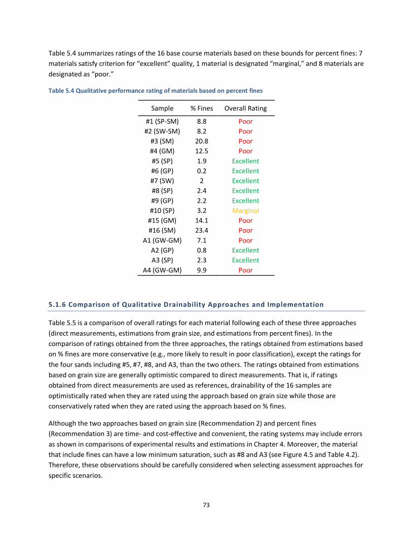
73
Table 5.4 summarizes ratings of the 16 base course materials based on these bounds for percent fines: 7
materials satisfy criterion for “excellent” quality, 1 material is designated “marginal,” and 8 materials are
designated as “poor.”
Table 5.4 Qualitative performance rating of materials based on percent fines
Sample % Fines Overall Rating
#1 (SP-SM) 8.8 Poor
#2 (SW-SM) 8.2 Poor
#3 (SM) 20.8 Poor
#4 (GM) 12.5 Poor
#5 (SP) 1.9 Excellent
#6 (GP) 0.2 Excellent
#7 (SW) 2 Excellent
#8 (SP) 2.4 Excellent
#9 (GP) 2.2 Excellent
#10 (SP) 3.2 Marginal
#15 (GM) 14.1 Poor
#16 (SM) 23.4 Poor
A1 (GW-GM) 7.1 Poor
A2 (GP) 0.8 Excellent
A3 (SP) 2.3 Excellent
A4 (GW-GM) 9.9 Poor
5.1.6 Comparison of Qualitative Drainability Approaches and Implementation
Table 5.5 is a comparison of overall ratings for each material following each of these three approaches
(direct measurements, estimations from grain size, and estimations from percent fines). In the
comparison of ratings obtained from the three approaches, the ratings obtained from estimations based
on % fines are more conservative (e.g., more likely to result in poor classification), except the ratings for
the four sands including #5, #7, #8, and A3, than the two others. The ratings obtained from estimations
based on grain size are generally optimistic compared to direct measurements. That is, if ratings
obtained from direct measurements are used as references, drainability of the 16 samples are
optimistically rated when they are rated using the approach based on grain size while those are
conservatively rated when they are rated using the approach based on % fines.
Although the two approaches based on grain size (Recommendation 2) and percent fines
(Recommendation 3) are time- and cost-effective and convenient, the rating systems may include errors
as shown in comparisons of experimental results and estimations in Chapter 4. Moreover, the material
that include fines can have a low minimum saturation, such as #8 and A3 (see Figure 4.5 and Table 4.2).
Therefore, these observations should be carefully considered when selecting assessment approaches for
specific scenarios.

74
Additional implementation into design software may also be considered. MnPAVE Flexible, for example,
consists of three design levels: basic, intermediate, and advanced. Design level is selected based on the
amount and quality of information known about the material properties, progressing from only general
knowledge in basic mode to advanced knowledge about material properties and environmental
operating range in advanced mode. By analogy, the three qualitative drainability approaches proposed
here can be considered as an input for: 1) advanced level when the rating system based on direct
measurements is applicable, 2) intermediate level when the rating system based on either grain size or
fines content is applicable, and 3) basic level when grain size index properties and fines content are not
available.
Table 5.5 Comparison of drainability assessments following three recommended approaches
Overall Rating
Sample Direct
Measurement Estimation from
Grain Size Estimation from
Percent Fines
#1 (SP-SM) Poor-Marginal Marginal Poor
#2 (SW-SM) Poor-Marginal Marginal Poor
#3 (SM) Poor Poor-Marginal Poor
#4 (GM) Marginal Poor-Marginal Poor
#5 (SP) Marg - Excellent Marginal Excellent
#6 (GP) Excellent Excellent Excellent
#7 (SW) Marginal Marg - Excellent Excellent
#8 (SP) Marginal Marg - Excellent Excellent
#9 (GP) Excellent Excellent Excellent
#10 (SP) Poor-Marginal Marg - Excellent Marginal
#15 (GM) Poor Poor Poor
#16 (SM) Poor Marginal Poor
A1 (GW-GM) Poor-Marginal Marginal Poor
A2 (GP) Excellent Marg - Excellent Excellent
A3 (SP) Marg - Excellent Marginal Excellent
A4 (GW-GM) Poor-Marginal Marginal Poor

75
REFERENCES
AASHTO. (1998). AASHTO guide for design of pavement structures. Washington, DC: American Association of State Highway and Transportation Officials.
AASHTO. (2007). Chapter 14 – Culvert inspection, material selection, and rehabilitation guideline. In Highway drainage guidelines (Fourth edition). Washington, DC: American Association of State Highway and Transportation Officials.
Alyamani, M. S., & Sen, Z. (1993). Determination of hydraulic conductivity from complete grain-size
distribution. Ground Water, 31(4), 551–555.
Barber, E. S., & Sawyer, C. L. (1952). Highway subdrainage. Public Roads, 26, 251–268.
Barr, D. W. (2001). Coefficient of permeability determined by measurable parameters. Ground Water,
39(3), 356–361.
Benson, C. H., Chiang, I., Chalermyanont, T., & Sawangsuriya, A. (2014). Estimating van Genuchten
parameters α and n for clean sands from particle size distribution data. Proceedings, From Soil
Behavior Fundamentals to Innovations in Geotechnical Engineering, M. Iskander, J. E.Garlanger,
& M. H.Hussein (Eds.): American Society of Civil Engineers (ASCE).
Beyer, W. (1964). Zur bestimmung der wasserdurchlassigkeit von kieson und sanduen aus der
kornverteilung [On the determination of hydraulic conductivity of gravels and sands from grain-
size distribution]. Wasserwirtschaft Wassertechnik, 14, 165–169.
Bouchedid, M. B., & Humphrey, D. N. (2005). Permeability of base material for Maine roads.
Transportation Research Record, 1936(1), 142–149.
Brooks, R. H., & Corey, A. T. (1964). Hydraulic properties of porous media (Hydrology paper No. 3, Civil Eng. Department). Fort Collins, CO: Colorado State University.
Campbell, G. S. (1985). Soil physics with basic. Amsterdam: Elsevier.
Campbell, G., & Shiozawa, S. (1992). Prediction of hydraulic properties of soils using particle size
distribution and bulk density data. Paper presented at the International Workshop on Indirect
Methods for Estimating the Hydraulic Properties of Unsaturated Soils, University of California
Press, Berkeley, CA.
Carman, P. C. (1937). Fluid flow through granular beds. Transactions, Institution of Chemical Engineers, 15, 150–166.
Carman, P. C. (1956). Flow of gases through porous media. London: Butterworths Scientific Publications.
Carsel, R. F., & Parrish, R. S. (1988). Variation within texture classes of soil water characteristics. Water Resource, 24, 755–769.

76
Carrier, W. D. (2003). Goodbye, Hazen; Hello, Kozeny-Carman. Journal of Geotechnical and
Geoenvironmental Engineering, 129(11), 1054–1056.
Cedergren, H. R. (1973). Development of guidelines for the design of subsurface drainage systems for highway pavement structural section (FHWA-RD-73-14. Office of Research), Washington, DC: Federal Highway Administration.
Cedergren, H. R. (1974). Drainage of highway and airfield pavements. New York: Wiley.
Cedergren, H. R. (1977). Seepage, drainage and flow nets. New York: Wiley.
Cedergren, H. R. (1994). America’s pavements: World’s longest bathtubs. Civil Engineering, 64, 56–58.
Celia, M. A., Bouloutas, E. T., & Zarba, R. L. (1990). A general mass-conserved numerical solution for the unsaturated flow equation. Water Resources Research, 26, 1483–1496.
Cetin, B., Coban, H., Edil, T., Ceylan, H., Likos, W., Zheng, J., Buss, A., (2021). Determining pavement design criteria for recycled aggregate base and large stone subbase (Final Report). St. Paul, MN: Minnesota Department of Transportation.
Chu, T. Y., Davidson, D. T., & Wickstrom, A. E. (1955). Permeability test for Sands ASTM Special Technical (Publication No. 1.63). Philadelphia, PA: American Society for Testing Materials.
Crank, J. (1984). Free and moving boundary value problems. Oxford, UK: Claredon Press.
Chapuis, R. P. (2004). Predicting the saturated hydraulic conductivity of sand and gravel using effective
diameter and void ratio. Canadian Geotechnical Journal, 41(5), 787–795.
Chapuis, R. P., Dallaire, V., Marcotte, D., Chouteau, M., Acevedo, N., & Gagnon, F. (2005). Evaluating the
hydraulic conductivity at three different scales within an unconfined sand aquifer at Lachenaie,
Quebec. Canadian Geotechnical Journal, 42, 1212–1220.
Domenico, P. A., & Schwartz, F. W. (1990). Physical and chemical hydrogeology. New York: Wiley.
Dungca, J. R., Galupino, J. G., Alday, J. C., Barretto, M. A. F., Bauzon, M. K. G., & Tolentino, A. N. (2018).
Hydraulic conductivity characteristics of road base materials blended with fly ash and bottom
ash. International Journal of GEOMATE, 14(44), 121–127.
Elhakim, A. F. (2016). Estimation of soil permeability. Alexandria Engineering Journal, 55(3), 2631–2638.
ERES. (1998). Evaluation of Unbonded Portland Cement Concrete Overlays (Final Report, NCHRP 10-41). Washington, DC: Transportation Research Board.
ERES. (1999). Pavement subsurface drainage design. (Reference manual ERES Project No. 99-035-E1). McLean, VA: U.S. Dept. of Transportation, Federal Highway Administration, National Highway Institute.
ERES. (2004). Guide for mechanistic-empirical design of new and rehabilitated pavement structures. Washington, DC: National Cooperative Highway Research Program, Transportation Research Board, National Research Council.

77
Espinoza, R. D., Bourdeau, P. L., & White, T. D. (1993). Pavement drainage and pavement shoulder joint evaluation and rehabilitation. Numerical analysis of infiltration and drainage in pavement systems. West Lafayette, IN: Purdue University.
Fair, G. M., & Hatch, L. P. (1933). Fundamental factors governing the stream-line flow of water through
sand. Journal of American Water Works Association, 25, 1551–1565.
FHWA. (1992). Drainable pavement systems: Participant notebook, demonstration project 87 (Publication No. FHWA-SA-92-008). Washington, DC: Federal Highway Administration (FHWA).
Fredlund, M. D., Wilson, G. W., & Fredlund, D. G. (2002). Use of the grain-size distribution for estimation
of the soil-water characteristic curve. Canadian Geotechnical Journal, 39(5), 1103–1117.
Fredlund, D. G., & Xing, A. (1994). Equations for the soil-water characteristic curve. Canadian
Geotechnical Journal, 31, 521–532.
Fu, H. Y., Wu, S. J., & Wang, G. Y. (2009). Experimental study of influence of compressive stress on water
permeability of sands soils (in Chinese). Rock and Soil Mechanics, 30(12), 3677–3681.
Ghanbarian-Alavijeh, B., Liaghat, A., Huang, G.-H., & Van Genuchten, M. T. (2010). Estimation of the van
Genuchten soil water retention properties from soil textural data. Pedosphere, 20(4), 456–465.
Green, R. E., & Corey, J. C. (1971). Calculation of hydraulic conductivity: A further evaluation of some predictive methods. Soil Science Society of America Journal, 35, 3–8.
Guyer, P. J. (2018). An introduction to subsurface drainage for pavements. El Macero CA: Guyer Partners
Hansen, V. E., Israelson, O. A., & Stingham, G. (1979). Irrigation principles and practice. New York: Wiley.
Harleman, D. R. F., Melhorn, P.F., & Rumer, R.R. (1963). Dispersion-permeability correlation in porous
media. Journal of the Hydraulic Division 89(2), 67–85.
Hazen, A. (1892). Some physical properties of sands and gravels, with special reference to their use in
filtration (24th annual report, 539–556). Boston, MA: Massachusetts State Board of Health.
James, L.G. (1988). Principles of farm irrigation system design. New York: Wiley.
Kern, J. S. (1995). Evaluation of soil water retention models based on basic soil physical properties. Soil Science Society of America Journal, 59(4), 1134–1141. https://doi.org/10.2136/sssaj1995.03615995005900040027x
Klink, T., (2021). Drainage characteristics of recycled materials for mechanically stabilized earth walls, (MS thesis). Madison, WI: University of Wisconsin-Madison.
Koerner, R. M. (1990). Designing with geosynthetics (Second edition). Englewood Cliffs, NJ: Prentice Hall.
Koenders, M. A., & Williams, A. F. (1992). Flow equations for particle fluid mixtures. Acta Mechanica,
92(1), 91–116.

78
Kozeny, J. (1927). Uber kapillare leitung des wassers in boden. Sitzungsber Akad (in German). Wiss. Wien
Mathematica Naturwiss K1, Abt.2a, 136, 271–306.
Kozeny, J. (1953). Das wasser im boden. grundwasserbewegung. Hydraulik, 380–445.
Kruger, E. (1918). Die grundwasserbewegung (in German). Internationale Mitteilungen fur Bodenkunde, 8, 105.
Krumbein, W. C., & Monk, G. D. (1943). Permeability as a function of the size parameters of
unconsolidated sands. Transactions of the American Institute of Mining, Metallurgical and
Petroleum Engineers, 151, 153–163.
Lenhard, R. J., Parker, J. C., & Mishra, S. (1989). On the correspondence between Brooks‐Corey and van
Genuchten models. Journal of Irrigation and Drainage Engineering, 115(4), 744–751.
Leong, E. C., & Rahardjo, H. (1997). Reviews of soil-water characteristic curve equations. Journal of
Geotechnical and Geoenvironmental Engineering, 123, 1106–1117.
LRRB. (2003). Effective methods to repair frost damaged roadways (Research implementation series Number 27). MN: Local Road Research Board.
Lu, C., Chen, X., Cheng, C., Ou, G., & Shu., L. (2012). Horizontal hydraulic conductivity of shallow
streambed sediments and comparison with grain-size analysis results. Hydrological Processes,
26, 454–466.
Lu, N., & Likos, W. J. (2004). Unsaturated soil mechanics. New York: Wiley.
Marianelli, F., & Durnford, D. S. (1998). Semi analytical solution to Richard’s equation for layered porous media. Journal of Irrigation and Drainage Engineering, 124, 290–299.
McEnroe, B. M. (1994). Drainability of granular bases for highway pavements. Transportation Research Record, 1434, 23–28.
MnDOT. (1994). Permeable aggregate base drainage systems - Design guidelines. St. Paul, MN: Materials Engineers Committee, Minnesota Department of Transportation.
MnDOT. (1995). Comparison of pavement drainage systems (Research report number Mn/RD–95/28). St. Paul, MN: Minnesota Department of Transportation.
MnDOT. (2002). Evaluation of water flow through pavement systems (Research report number Mn/RC–2002-30). St. Paul, MN: Minnesota Department of Transportation.
MnDOT. (2003a). Special practices for design and construction of subgrades in poor, wet and/or saturated soil conditions (Research report number Mn/RC–2003-36). St. Paul, MN: Minnesota Department of Transportation.
MnDOT. (2003b). Designing pavement drainage systems: The MnDRAIN Software (Research report number Mn/RC–2003-17). St. Paul, MN: Minnesota Department of Transportation.

79
MnDOT. (2009a). Evaluating roadway subsurface drainage practices (Research report number MN/RC 2009–08). St. Paul, MN: Minnesota Department of Transportation.
MnDOT. (2009b). Subsurface drainage manual for pavements in Minnesota (Research report number MN/RC 2009–17). St. Paul, MN: Minnesota Department of Transportation.
MnDOT. (2012). A Research plan and report on factors affecting culvert pipe service life in Minnesota (Research report number MN/RC 2012–27). St. Paul, MN: Minnesota Department of Transportation.
Mokwa, R. L., & Trimble, N. R. (2008). Permeability of coarse-grain soil from void space and pore
distribution. Paper presented at GeoCongress 2008, New Orleans, LA.
Moulton, L. K. (1980). Highway subsurface drainage design (FHWA-TS-80-224). Washington, DC: Office of Research and Development, Federal Highway Administration.
Navfac DM7. (1974). Design manual—Soil mechanics, foundations and earth structures. Washington, DC:
U.S. Government Printing Office.
NYDOT. (1973). Test procedures for specific surface analysis soil test procedures STP-1. New York: Soil Mechanics Bureau.
Oh, Y., Hamm, S., Chung, S. Y., & Lee, B. D. (2013). Characterizing hydraulic properties by grain-size analysis of fluvial deposits depending on stream path in Korea. Environmental Engineering Research, 18(3), 129–137, https://doi.org/10.4491/eer.2013.18.3.129
Pineda, M. C., Viloria, J., Martínez-Casasnovas, J. A., Valera, A., Lobo, D., Timm, L. C., Pires, L. F., &
Gabriels, D. (2018). Predicting soil water content at − 33 kPa by pedotransfer functions in
stoniness 1 soils in northeast Venezuela. Environmental Monitoring and Assessment, 190(161),
https://doi.org/10.1007/s10661-018-6528-3
Pravedny, G. H. (1966). Design and selection of grain size composition of filter beds for the transition
zones of large dams. Moscow: Energiia.
Rawls, W. J., Ahuja, L. R., Brakensiek, D. L., & Shirmohammadi, A. (1992). Soil water movement and infiltration. In Handbook of hydrology. New York: McGraw Hill.
Ren, X., Zhao, Y., Deng, Q., Kang, J., Li, D., & Wang, D. (2016). A relation of hydraulic conductivity — void
ratio for soils based on Kozeny-Carman equation. Engineering Geology, 213, 89–97.
Richards, L. A., & Weaver, L. R. (1944). Moisture retention by some irrigated soils as related to soil-moisture tension. Journal of Agricultural Research, 69(6), 215–235.
Robertson, P. K. (2010). Estimating in-situ soil permeability from CPT & CPTu. Paper presented at the
2nd International Symposium on Cone Penetration Testing, Huntington Beach, CA.
Rosas, J., Lopez, O., Missimer, T. M., Coulibaly, K. M., Dehwah, A. H. A., Sesler, K., & Mantilla, D. (2013).
Determination of hydraulic conductivity from grain-size distribution for different depositional
environments. Groundwater, 52(3), 399–413.

80
Salarashayeri, A. F., & Siosemarde, M. (2012). Prediction of soil hydraulic conductivity from particle-size
distribution. World Academy of Science Engineering and Technology, International Journal of
Geological and Environmental Engineering, 6(1), 16–20.
Seelheim, F. (1880). Methoden zur bestimmung der durchlässigkeit des bodens (in German). Zeitschrift
für Analytische Chemie, 19, 387–418.
Sillers, W. S., Fredlund, D. G., & Zakerzadeh, N. (2001). Mathematical attributes of some soil-water
characteristic curve models. Geotechnical and Geological Engineering, 19, 243–283.
Singh, V. P. (1997). Kinematic wave modeling in water resources: Environmental hydrology. New York:
Wiley.
Slichter, C. S. (1899). Theoretical investigation of the motion of ground waters. (U.S. Geological Survey
19th annual report, Part 2: 322). Reston, VA: USGS.
Smith, K. D., Mueller, A. L., Darter, M. I., & Peshkin, D. G. (1990). Performance of jointed concrete pavements, Volume II - Evaluation and modification of concrete pavement design and analysis models. McLean, VA: Federal Highway Administration.
Stephens, D. B., Hsu, K., Prieksat, M. A., Ankeny, M. D., Blandford, N., Roth, T. L., Kelsey, J. A., & Whitworth, J. R. (1998). A comparison of estimated and calculated effective porosity. Hydrogeology Journal, 6, 156–165, https://doi.org/10.1007/s100400050141
Terzaghi, C. (1925). Principles of soil mechanics. Engineering News Record, 95, 832.
Trzebiatowski, B., & Benson, C. (2005). Saturated hydraulic conductivity of compacted recycled asphalt
pavement. Geotechnical Testing Journal, 28(5), 514–519.
Tinjum, J., Benson, C., & Blotz, L. (1997). Soil-water characteristic curves for compacted clays. Journal of
Geotechnical and Geoenvironmental Engineering, 123(11), 1060–1069.
van Genuchten, M. T. (1980). A closed form solution for predicting the hydraulic conductivity of
unsaturated soil. Soil Science Society of America Journal, 11, 892–898.
van Genuchten, M. T., Leij, F. J., & Yates, S. R. (1991). The RETC code for quantifying the hydraulic
functions of unsaturated soils (Report IAG-DW 12933934). Riverside, CA: U.S. Department of
Agriculture, Agricultural Research Service.
Vauclin, M., Khanji, D., & Vachaud, G. (1979). Experimental and numerical study of a transient two
dimensional unsaturated-saturated water table recharge problem. Water Resources Research,
15(5), 1089–1101.
Vukovic, M., & A. Soro. (1992). Determination of hydraulic conductivity of porous media from grain-size
composition. Littleton, CO: Water Resources Publications.

81
Wan, L., Jiang, X. W., & Wang, X. S. (2010). A common regularity of aquifers: The decay in hydraulic
conductivity with depth (in Chinese). Geological Journal of China Universities, 16(1), 7–12.
Wang, J. P., François, B., & Lambert, P. (2017). Equations for hydraulic conductivity estimation from
particle size distribution: A dimensional analysis. Water Resources Research, 53(9), 8127–8134.
Wraith, J. M., & Or, D. (1998). Nonlinear parameter estimation using spreadsheet software. Journal of
Natural Resources and Life Sciences Education, 27, 13–19.
Zhang, G. L., & Wang, Y. J. (2014). Experimental investigation of hydraulic conductivity of sand under
high confining pressure (in Chinese). Yantu Lixue/Rock and Soil Mechanics, 35(10), 2748–2754.
Zienkiewicz, O. C., & Taylor, R. L. (1989). The finite element method (Fourth edition). New York: McGraw-
Hill.

APPENDIX A
CASE HISTORY REVIEW

A-1
Case histories summarized here were primarily focused on evaluating subsurface drainage systems
based on literature reviews, surveys, experiments, numerical modeling, and statistical analyses. Review
of these studies provides theoretical and practical background for the current research project.
Emphasis is placed on research on pavement systems performed by the Minnesota Department of
Transportation (MnDOT).
A.1 EVALUATION OF WATER FLOW THROUGH PAVEMENT SYSTEMS (MNDOT, 2002)
Pavement systems can be fully saturated only under very specific circumstances, such as surface
ponding where positive total heads are present and distributed in such a manner that saturation of the
pavement system is reached. Drainage design criteria used in the past has predominantly assumed the
flow of water through pavements and the drainage of pavement layers can be represented with
saturated flow. In this research project, unsaturated water flow in three testing sections, MnROAD Cell
33, Cell 34, and Cell 35, was numerically modeled using SEEP/W to represent the first step in the
development of a comprehensive approach considering the unsaturated soil condition. Results of the
SEEP/W modeling were compared with experimental results and analytical solutions calculated using
Drainage Requirements In Pavements (DRIP) from the Federal Highway Administration (FHWA).
Prior to modeling for the testing sections, experimental results and analytical solutions in Espinoza et al.
(1993) and Vauclin et al. (1979) were compared with SEEP/W predictions to evaluate use of SEEP/W for
modeling the water flow through soils and simplified pavement systems. Comparison of results for three
example cases showed that SEEP/W is a useful tool for the modeling of unsaturated flow through
layered systems under complex boundary conditions and material characterization.
For material properties of the three testing sections used in the modeling, soil-water characteristic
curves (SWCCs) and hydraulic conductivity functions (HCF) for base material, Class 6 special material,
and subgrade soil, R-12 silty clay, were measured using the suction plate testing (Figure A.1). The air-
entry pressures in SWCCs were shifted to 3 kPa for the modeling. A saturated hydraulic conductivity of
1.54E-6 m/s was obtained from Figure A.1(c). In addition, using automated time domain reflectometry
(TDR) probes, volumetric water contents were measured in the base layer at 0.13 m (101), 0.25 m (102),
and 0.38 m (103) depth. The measured TDR volumetric water contents were used as benchmarks for
adjusting laboratory-based unsaturated soil hydraulic properties.

A-2
(a)
(b)
(c)

A-3
(d)
Figure A.1 Material properties used in the modeling: (a) soil-water characteristic curve for base material (Class 6
special), (b) soil-water characteristic curve for subgrade soil (R-12 silty clay), (c) hydraulic conductivity curve for
base material (Class 6 special), and (d) hydraulic conductivity curve for subgrade soil (R-12 silty clay)
The three sections consisted of a layer of hot mix asphalt (i.e., impervious material), a Mn/DOT Class 6
Special base course (consisting of 100 percent crushed granite), and an R-12 silty clay subgrade (Figure
A.2). A time-dependent flux boundary condition was applied on the shoulder to simulate infiltration
from precipitation. Rain events (time-dependent flux condition) were applied on top of the base, and
the ones underneath the hot mix asphalt represent no infiltration through this material [Figure A.2(a)].
To represent real conditions more accurately, the subgrade layer was extended laterally 10 m beyond
the area covered by the asphalt and base layer [Figure A.2(b)]. To induce lateral and vertical drainage in
the system, points of total head equal to 0 m were applied at the bottom corners.
(a)

A-4
(b)
Figure A.2 Geometry and mesh used in the modeling: (a) section representing Cells 33, 34, and 35 and (b)
extended subgrade layer
Figure A.3 shows the measured TDR water contents for each cell. For a more detailed and definitive
comparison between measured and predicted results, the span of time from July 31st to September 30th,
2000 was chosen for this study. Although the range is 22 days shorter than the precipitation data, the
first 22 days established an initial volumetric water content baseline in the model.
(a)

A-5
(b)
(c)
Figure A.3 Volumetric water content obtained from TDR probes: (a) at Cell 33, (b) at Cell 34, and (c) at Cell 35
As volumetric water contents predicted from SWCCs [Figures A.1(a) and (b)] were slightly different from
the TDR field volumetric moisture contents due to limitations (e.g., the required empirical calibration of
results, differences in field and laboratory compaction processes), SWCCs were adjusted to fit the TDR
field data based on the air entry values, saturated volumetric water content, and the slope of the
SWCCs. After the calibrations, hydraulic conductivity curves were generated using the Green and Corey
(1971) formulation in SEEP/W. These procedures were used to simulate changes in volumetric water
contents for Cells 33, 34, and 35 at TDR locations 101, 102, and 103. Figure A.4 shows Cell 34 results as
examples, and the results were well aligned.

A-6
(a)
(b)
(c)
Figure A.4 Comparisons of volumetric water contents obtained at Cell 34: (a) TDR location 101, (b) TDR location
102, and (c) TDR location 103

A-7
In addition, sensitivity analyses were conducted using Cell 33 at TDR location 101 (as a representative
pavement configuration) for evaluating effects of : 1) the initial slope of the soil water characteristic
curve, 2) the air entry value of the Mn/DOT Class 6 Special crushed granite, 3) the saturated hydraulic
conductivity of the Mn/DOT Class 6 Special crushed granite, 4) the air entry value of the R-12 silty clay
subgrade soil, 5) the saturated hydraulic conductivity for the subgrade soil, 6) the type of granular base
material, 7) variations in infiltration characteristics, and 8) the water table location. The results indicated
that the most sensitive parameters were as follows: 1) the air entry value of the granular base course
material, 2) water table location, and 3) gradation and type of Mn/DOT Class granular base material.
Similarly, moderate sensitivity was observed with changes in saturated hydraulic conductivity of the
subgrade and time history of infiltration. Finally, the volumetric moisture content was found to be
relatively insensitive to changes in the initial slope of the soil water characteristic curve, the saturated
hydraulic conductivity of the granular base material, and the air entry value for the subgrade soil.
Lastly, in this research project, effects of edge and under drains on the water flow were evaluated. The
edge drain consists of coarse graded gravel surrounding a collector pipe in trench that is longitudinally
placed next to the outer traffic lane under the shoulder. The under drain consists of a layer of a woven
or non-woven geotextile that extends all the way under the traffic lanes to replace an equivalent sand
drainage layer. The numerical modeling for Cell 33 was used as a baseline with four drainage systems: 1)
the original pavement section for Cell 33 with a 0.02 m thick geotextile underdrain located between the
Mn/DOT Class 6 Special crushed granite base course and the subgrade soil, 2) modification of Case 1, in
which collector pipes were placed directly in the Mn/DOT Class 6 Special crushed granite coarse base
material under the shoulder, 3) a typical edge drain configuration from Cell 10, and 4) a combination of
an edge drain and a geotextile under drain system, in which the under drain now connects to a
backfilled trench containing a collector pipe. The main difference between Case 2 and Case 4 was that
the material around the collector pipe (Case 2) was Class 6 Special crushed granite, while the material
around the edge drain consisted of well-draining gravel (pea gravel). The results indicated that under
drains did not significantly improve the drainability of dense graded bases, while either collector pipes
or edge drains in combination with under drains was very effective to reduce the amount of moisture in
a Mn/DOT Class 6 Special crushed granite base course material. This was because of the effects of zero
head boundary conditions around the collector pipes and edge drains, which in combination with the
shortened drainage path due to the under drains affected the distribution of suctions significantly
throughout the base material, thus promoting better drainage.
A.2 DESIGN AND CONSTRUCTION OF SUBGRADES IN POOR, WET, AND/OR SATURATED
SOIL CONDITIONS (MNDOT, 2003A)
In constructions of pavement structures the subgrade soil helps resist the destructive effects of traffic
and weather (MnDOT, 2003a). For the subgrade, naturally occurring soils have been used due to various
benefits (e.g., cost-effective, easier access). However, the subgrade based on natural soil sometimes has
mechanically and physically poor conditions that should be improved. In this research project, literature

A-8
review, questionnaire directed to Minnesota state, county, and city highway engineers, and interviews
were thus conducted to provide enhanced methods for the subgrade.
MnDOT (2003a) summarizes various traditional subgrade enhancement choices: 1) surface (e.g.,
pavement) drainage of runoff and subsurface (e.g., embankment) drainage of infiltrated water, 2)
compaction using heavy equipment, 3) moisture content adjustment through mechanical or chemical
methods, 4) soil modification with cementing or drying agents (e.g., lime, fly ash, bituminous), 5) soil
stabilization with cementing or drying agents (e.g., Portland cement, lime, fly ash), 6) reinforcement and
separation using geosynthetics (e.g., geotextile, geogrid, geomembrane), and 7) substitution with
natural (granular, wood) or man-made materials (shredded tires, form). Compatibility with in-service
subgrade soil conditions, extent of improvement required, safety precautions or environmental
concerns, and construction requirements should be considered to appropriately select the enhancement
method.
Drainage refers to the removal of surface and/or subsurface water, such as drawdown of the water
table, intercepting lateral seepage above an impervious pavement layer, drain of infiltrating surface
water, and preventing capillary rise or collecting discharge from other drainage systems. Proper
drainage helps maintain the pavement strength due to a decrease in pore water pressure (i.e., increased
inter-particle friction) and minimizes frost heave and thaw weakening. The surface drainage is achieved
using storm sewers, ditches, culverts, or bridges, and the subsurface drainage is accomplished through
uses of permeable base, pipes, drains, and geosynthetics.
There are two common drainage systems for subgrade enhancement: longitudinal edge drains and
permeable base layer. Effectiveness and performance of the longitudinal drains and the permeable base
are dependent on filter materials, pipes, location of seepage area within the system, and soil
permeability. For example, permeable asphalt stabilized base (PASB), which has a permeability
coefficient of 300 m/day, drained the most water within 2 hours of the end of rainfall (MnDOT, 1995).
According to MnDOT (2003a), permeable bases may be treated with asphalt (2 – 5 % by weight) or
Portland cement (2 – 3 bags/cubic yard) for strength in construction. A separator layer should be
installed a minimum depth of 4 in. (102 mm) below the permeable base to prevent the migration of fine
aggregate particles. Aggregate should have a dense gradation, and there are uniformity requirements as
follows:
𝐷15
𝐷85 of
𝑓𝑖𝑙𝑡𝑒𝑟
𝑠𝑢𝑏𝑔𝑟𝑎𝑑𝑒 and
𝑏𝑎𝑠𝑒
𝑓𝑖𝑙𝑡𝑒𝑟≤ 5 (A.1)
𝐷50
𝐷50 of
𝑓𝑖𝑙𝑡𝑒𝑟
𝑠𝑢𝑏𝑔𝑟𝑎𝑑𝑒 and
𝑏𝑎𝑠𝑒
𝑓𝑖𝑙𝑡𝑒𝑟≤ 25 (A.2)
20 ≤𝐷60
𝐷10≤ 40 (A.3)
where 𝐷15 = Maximum particle size at which 15 percent of the aggregate is finer, 𝐷50 = Maximum
particle size at which 50 percent of the aggregate is finer, 𝐷85 = Maximum particle size at which 85
percent of the aggregate is finer.

A-9
For pavement applications in Minnesota, various geosynthetics are used as a separation of dissimilar
materials, a subgrade enhancement, a drainage application, and for filtration in the drainage system.
Specifically, geomembrane, which is a relatively impermeable barrier due to the low permeability of
water vapor for geomembrane (5 × 10-11 to 5 × 10-14 cm/s), is used for the separation between an
underlying fine-grained soil and an aggregate base or granular subbase. Geogrid is commonly used to
reduce deformation and improve the durability and lifespan of paved roads, primarily due to an increase
in stiffness and the load spreading ability of geogrids. Geonet, which is similar to the geogrid except
larger apertures, is used for drainage application. The drainage performance is dependent on the
thickness (ASTM D1777) and can be degraded over time due to clogging of soil particles, destruction at a
high temperature, and damages caused by chemical reactions. Lastly, in the drainage system, small
aperture of the geotextiles keeps large particles from entering the drainage layer or pipe, allowing some
of the small, suspended particles to pass without clogging.
There are three major design components for a geosynthetic drainage system: 1) maximum flow rate
necessary to drain area, 2) percent and size of fine-grained material, and 3) type of drain system to be
implemented. The maximum aperture of the geosynthetic must be smaller than the larger particles in
the soil, retaining a majority of the soil, and use of transmissivity values will help ensure adequate flow
with proper soil retention.
Table A.1 Typical values of transmissivity (in-plane drainage capability) of geotextiles (Koerner, 1990)
Type of Geotextile Transmissivity (m2/s) Permeability (m/s)
Nonwoven, heat-bonded 3.0 × 10⁻⁹ 6 × 10⁻⁶ Woven, slit-film 1.2 × 10⁻⁸ 2 × 10⁻⁵
Woven, monofilament 3.0 × 10⁻⁸ 4 × 10⁻⁵ Nonwoven, needle-punched 2.0 × 10⁻⁶ 4 × 10⁻⁴
*Values taken at applied normal stress of 40 kPa
In addition to the geosynthetics, shredded tires have been used as a lightweight fill and drainage layers
(hydraulic conductivity of tire shreds is 1 cm/sec). As tire shreds have a compacted dry density of one-
third to one-half of the compacted dry density of a typical soil, the tires are attractive lightweight fill for
construction on weak and compressible soils where slope stability or excessive settlement is concerned.
Due to the low thermal conductivity of tire shreds, the tires can be used as an insulating layer of 6 in.
(150 mm) to 18 in. (450 mm) thickness.
A.3 DESIGNING PAVEMENT DRAINAGE SYSTEMS: THE MNDRAIN SOFTWARE (MNDOT,
2003B)
Edge drain is a drainage used in a road system to remove moisture from the granular base through pipes
placed in a gravel trench. To evaluate a quality of the edge drain, for the first step, time to drain the
moisture from 100% to 85% saturation is calculated. The calculations are then used to evaluate the
drainage quality based on pavement rehabilitation manual guidance of federal highway administration
(e.g., excellent = less than 2 hours, good = 2 to 5 hours).

A-10
In this research project, MnDrain codes were outlined for a design of the edge drain. Figure A.5 shows
the drainage system used for developing MnDrain codes. The system consisted of two materials: fine
material that has a low saturated hydraulic conductivity and coarse material that has a relatively higher
saturated hydraulic conductivity.
Figure A.5 schematic layered drainage system
For the calculations, mixed form of Richard equations that describe the moisture migration in variably
saturated soil was solved using control volume finite element method (CVFE), which is a combination of
the finite element and finite volume methods.
𝜕𝜃
𝜕𝑡= ∇ ∙ (𝐾(ℎ)∇ℎ) +
𝜕𝐾
𝜕𝑧 (A.4)
where 𝜃 = moisture content (a function of pressure head), ℎ = pressure head (negative in the
unsaturated region), 𝐾 = hydraulic conductivity (a function of pressure head). The pressure head, ℎ, is
defined as follows:
ℎ =𝑃
𝛾 (A.5)
where 𝑃 = pressure, 𝛾 = specific weight of water. The pressure, 𝑃, is equal to the minus of the suction
pressure. In terms of the moisture content, the pressure head has three states: 1) ℎ ≥ 0 when all voids
are filled with moisture (𝜃 = 𝜃𝑠𝑎𝑡), 2) ℎ < 0 when all voids are filled by capillary action (the moisture
content is still 𝜃 = 𝜃𝑠𝑎𝑡), and 3) ℎ < 0 when 𝜃𝑟𝑒𝑠 < 𝜃(ℎ) < 𝜃𝑠𝑎𝑡 , where 𝜃𝑟𝑒𝑠 = residual moisture
content (ℎ → −∞).

A-11
In addition to Richard equation (Equation A.4), there are two auxiliary relationships among the moisture
content, hydraulic conductivity, and pressure head: Brooks Corey (1964) and van Genuchten (1980).
Brooks Corey (1964)
𝜃 = {(𝜃𝑠𝑎𝑡 − 𝜃𝑟𝑒𝑠)(ℎ/ℎ𝑑)−𝜆1 + 𝜃𝑟𝑒𝑠 , ℎ < ℎ𝑑
𝜃𝑠𝑎𝑡 , ℎ > ℎ𝑑 (A.6)
𝐾 = 𝐾𝑠𝑎𝑡 [𝜃−𝜃𝑟𝑒𝑠
𝜃𝑠𝑎𝑡−𝜃𝑟𝑒𝑠]
𝜆2
(A.7)
where 𝜆 = material constant.
van Genuchten (1980)
𝜃 = {𝜃𝑠𝑎𝑡−𝜃𝑟𝑒𝑠
(1+|𝛼ℎ|𝑛)𝑚 + 𝜃𝑟𝑒𝑠 ℎ < ℎ𝑑
𝜃𝑟𝑒𝑠 ℎ > ℎ𝑑
(A.8)
𝐾 = 𝐾𝑠𝑎𝑡 [𝜃−𝜃𝑟𝑒𝑠
𝜃𝑠𝑎𝑡−𝜃𝑟𝑒𝑠]
0.5[1 − (1 − [
𝜃−𝜃𝑟𝑒𝑠
𝜃𝑠𝑎𝑡−𝜃𝑟𝑒𝑠]
1/𝑚)
𝑚
]
2
(A.9)
where 𝛼, 𝑚, 𝑎𝑛𝑑 𝑛 = material parameters.
In this study, the Brooks Corey equations were used with an artificial relationship, 𝐶𝑣𝑎𝑙, to form a
solution of the non-linear equations resulting from a discretization of the equation:
𝜃 = {(𝜃𝑠𝑎𝑡 − 𝜃𝑟𝑒𝑠)(ℎ/ℎ𝑑)−𝜆1 + 𝜃𝑟𝑒𝑠 , 𝑓𝑜𝑟 ℎ < ℎ𝑑
𝐶𝑣𝑎𝑙(ℎ − ℎ𝑑) + 𝜃𝑠𝑎𝑡 , 𝑓𝑜𝑟 ℎ ≥ ℎ𝑑 (A.10)
If the constant 𝐶𝑣𝑎𝑙 is small enough (10-4 was used in this study), this extended definition has a minimal
impact on the results, allowing a continuous relationship between 𝜃 and ℎ throughout the solution.
According to MnDOT (2003b), a rapid change in the moisture content cannot be treated well using the
Richards equation (Equation A.4), possibly involving discontinuous hydraulic conductivity. The equation
A.4 was thus incorporated with a Kirchoff transformation (Crank, 1984) and can be rewritten as follows:
𝜕𝜃
𝜕𝑡= ∇2𝜑 +
𝜕𝐾
𝜕𝑧 (A.11)

A-12
where 𝜑 = ∫ −𝐾(𝛼)ℎ
0𝑑𝛼. The governing equation (Equation A.11) was solved using CVFE method, and
the first step was generating a mesh of triangular elements that covers the two-dimensional domain
with node points located at vertices (Figure A.6). An interface between two layers of material in the
drain lies along element edges.
Figure A.6 Basic components in a control volume finite element solution
In each element, an unknown 𝜑 is approximated by
𝜑(𝑥, 𝑧) = 𝑁1𝜑1 + 𝑁2𝜑2 + 𝑁3𝜑3 (A.12)
where 𝑁 = linear function of x and y arranged such that NP takes the value of unity at node P and
vanishes on the line segment opposite node P (Zienkiewicz and Taylor, 1989). Within this arrangement, a
control volume is constructed where the mid points of the element sides are connected to the element
centers. Balancing the fluxes across the faces of the control volumes arrives at an algebraic (discrete)
Equation A.11 as follows:
𝐴𝑃�̅�𝑃 − 𝐴𝑃�̅�𝑃,𝑜𝑙𝑑 = ∆𝑡 ∑ [𝑎𝐼(𝜑𝐼 − 𝜑𝑃) + 𝑆𝐼]𝐼 (A.13)
where 𝐼 = a counter over the nodes in the grid connected to node P, 𝑎𝐼 = coefficient, 𝑆𝐼 = contribution to
the source term that can be associated with node 𝐼. The Equation A.13 can be rewritten in terms of total
head.
𝐴𝑃�̅�𝑃 = 𝐴𝑃�̅�𝑃,𝑜𝑙𝑑 + ∆𝑡 ∑ 𝐾𝐼𝑒𝑎𝐼
𝑒(ℎ𝐼 − ℎ𝑃) + 𝑆𝐼𝐼 (A.14)

A-13
where the sum is over the nodes connected to node P, and each component in the sum includes
contributions from both the elements that share the common side between nodes P and I. The
discretized equation (Equation A.14) can be solved using the linearization introduced by Celia et al.
(1990).
A set of test problems was simulated using MnDrain software and commercial codes, and the results
were compared to verify the MnDrain codes (Figure A.7). Figure A.7(a) presents the results for draining a
layered column obtained from MnDrain software and Marianelli and Durnford solutions that the
accuracy is not lost in regions of rapid change in the solution fields (Marianelli and Durnford, 1998). The
result obtained from MnDrain reasonably predicted the sharp discontinuity at the layer interface
without leaking. In comparisons of the results for two-dimensional infiltration into a homogeneous
domain [Figure A.7(b)], the results were well aligned, clearly indicating that the correct treatment of
infiltration is implemented in MnDrain. The last test problem was designed to simulate drainage in a
two-dimensional layered system. The moisture contents at interfaces were calculated based on the
pressure [Figure A.7(d)], and the results were well aligned [Figure A.7(c)].
(a)

A-14
(b)
(c)
(d)
Figure A.7 Comparisons of simulation results for (a) draining a layered column, (b) infiltration into a two-
dimensional homogeneous domain, (c) boundary moisture profiles in two-dimensional layered domain, and (d)
pressure head history at layer interface in two-dimensional layered domain

A-15
Figure A.8 Schematic of edge drain system
Figure A.8 shows an edge drain system used for MnDrain solution domain. The geometry consists of an
initially saturated base, drain trench, and edge drain on a permeable sub-grade with an adjustable water
table height. Initial condition of the solution domain was fully saturated with h = 0. Most of the
boundary conditions are no flow conditions, except two boundary conditions: 1) The water table, at the
bottom of the domain, where a fixed pressure head of h = 0 is applied and 2) the drain pipe surface in
the trench where a review boundary condition is applied. In the initial stages of the calculation nodes on
the drainpipe, a fixed pressure head of h = 0 needs to be taken. If this condition leads to an influx of
moisture into the trench, this fixed head condition is replaced by a no flow condition at that node.
A.4 EFFECTIVE METHODS TO REPAIR FROST DAMAGED ROADWAYS (LRRB, 2003)
Cold weather in Minnesota is the only factor affecting pavement performance that human cannot
modify or mitigate. Regarding the cold weather, there are two natural phenomena that damage the
pavement system: 1) frost heave that is the expansion and heaving of frost-susceptible subgrade
materials as they freeze and 2) frost boil that is the subsequent weakening of those materials as they
thaw in spring, which decreases their load-carrying capacity. To provide effective methods to repair the
frost damaged roadways, local road research board (LRRB) conducted the literature review and e-mail
survey of local governments and developed worksheet and flow chart. To be specific, this research
report includes discussions for the mechanics of ground freezing and frost related roadway damage, the
environments in which such damage occurs, and measures to evaluate the contributing factors along
with recommendations to mitigate them and/or reduce the potential for additional roadway damage.
Subgrade composition, groundwater condition, and drainage quality are key components of the frost
related roadway damage, and the areas where the road damage occurs can be defined, in terms of the
three components, by three categories: non-uniform subgrades, subgrades near the groundwater,
subgrades within low areas. Typically, fine-grained soils, including lean and fat clay, silty clay, non-
plastic, fine sands with silt, and elastic silt, are considered as frost-susceptible soils due to the low
hydraulic conductivity and the high matric suction. That is, the non-uniform subgrade that locally
includes fine-grained soils can cause differential frost heaving and frost boils. Near the groundwater (or
local water features, such as lakes and swamps), the frost-susceptible soils also can be expanded due to
formations of ice lenses when frozen is largely affected by the capillary action. Lastly, the frost related

A-16
road damage can be occurred in subgrades within low areas where water is accumulated (e.g., the
accumulation of surface drainage in ditches at low points along a roadway passing through rolling
terrain).
There are various repair methods and alternatives to mitigate and repair the frost damage. To
appropriately select the treatment option, for the first step, prospective repair alternatives are needed
to be evaluated by four steps: 1) construction/maintenance history, 2) visual observation, 3) subgrade
evaluation (pavement deflection testing, penetration test borings or auger borings, dynamic cone
penetrometer testing), and 4) construction materials. After the assessment of site-specific issues, the
following repair methods should be uniquely selected for the site that has unique conditions:
1) Scarification, blending and re-compaction: suited for situations where subgrade uniformity
appears to be more critical than groundwater or surface drainage,
2) Removal, surface compaction and re-compaction: suited for frost heave rather than frost boil
repair where the loss of support to the paved surface is limited,
3) Removal and replacement: suited for non-uniform areas where both frost heaves and frost boils
are present and situations where the extent and/or magnitude of frost damage is strongly
influenced by shallow groundwater trapped in layered soils and present in low areas,
4) Northern Minnesota practice: cost-effective practice that uses woven or non-woven geotextile
covered with 8 to 12 inches of granular material,
5) Embankment modification: in shallow groundwater situations or in low areas, raising the
existing alignment provides sufficient clearance to i) reduce the impact that groundwater and
infiltrating subsurface drainage has on subgrade stability and pavement performance, ii) reduce
the extent to which excavations need to be advanced into wet, saturated or potentially unstable
materials, and iii) support pavement materials on a uniform cushion of higher quality material
than may have existed,
6) Transitions: material transitions (e.g., replacing weak or poorly draining subgrade materials with
higher strength or more free-draining subgrade materials) can cause unfavorable amounts of
differential frost heave. Tapering the edges of corrective excavations (e.g., 4:1 taper for general,
5:1 taper for a low-volume city street, 20:1 taper for highway repair) is thus required to reduce
potential differential movements,
7) Constructability – stabilization, separation and reinforcement: general subgrade or excavation
bottom stabilization can be achieved with the aid of chemical additives such as lime or fly ash,
which absorb excess moisture and facilitates compaction. Geosynthetics (e.g., non-woven and
woven geotextiles or geogrids) also can be placed over excavation bottoms to achieve subgrade
stability and limit the migration of fine-grained subgrade particles into coarse-grained backfills,
8) Considerations for alternative subgrade materials: other synthetic and structural products, such
as Geofoam®, shredded or chipped tires, wood chips, geocells, are available to help solve frost
damage problems.
Finally, there are two strategies to reduce and limit subgrade moisture: surface drainage and subsurface
drainage. The magnitude of subgrade heaving upon freezing and strength loss upon thawing can be
significantly reduced by surface drainage systems. The surface drainages in urban areas include storm

A-17
drainage systems and the installation of curb and gutter. In rural areas, pavements are sloped to drain
into ditches that ultimately carry water into streams, lakes, swamps or other low areas. Groundwater
movement and percolation of surface drainage into pavement subgrades can saturate and weaken the
subgrades. For outlets of water in the subgrade, drainpipes are installed below free-draining subbase
layers or below the aggregate base layer where a subbase is not provided.
A.5 EVALUATING ROADWAYS SUBSURFACE DRAINAGE PRACTICES (MNDOT, 2009A)
This research project evaluated the efficacy of drainage systems of roadway base materials in a newly
constructed eight-mile section of County Sate Aid Highway No. 35 (CSAH 35) in Nobles County, MN,
based on experiments. The experiments included three drainage treatments: 1) drains on the roadway
edge, 2) drains along the roadway centerline at depth of 2 ft., and 3) drains along the roadway
centerline at depth of 4 ft, and each of the configurations was replicated six times, with the outflow for
each replication outlet through a tipping-bucket flow monitoring system. The results were examined
whether the elevation of the roadway relative to the surrounding landscape or the orientation of the
drains at either side of the road had a significant impact on the efficacy of the drain. The CSAH 35 was
separated into 87 sections (500-feet long for each section), and the 87 sections were divided into three
sample populations: 1) 37 sections for relatively flat highway sections, 2) 23 sections for sloping section
(about 1% - 3% slope), and 3) 27 sections for culverts and/or road intersections. Among 37 sections in
the first population, 30 sections were randomly chosen for one of the three drainage treatments. From
the second population, 10 sections were chosen for edge drains.
Tipping bucket device was buried at or near ground level (for safety precaution) to directly monitor a
volume of the water flow. The results indicated edge drains collected much more water than the other
two centerline drains combined during the two-year period (2006-2007). Volumes collected during both
March and April were considerably higher than those of the other months. In result comparisons for the
effect of install elevations, in general, drains at the lower elevation had a higher drain volume during
March and April monitoring periods, but those during the rest of the year the drainage volumes did not
show the tendency that depends on the elevation.
In addition to the tipping bucket apparatus, EM38, which is an electromagnetic induction instrument,
was used to indirectly obtain relative moisture content of the subgrade material. Specifically, EM38
measured electrical conductivity of the subgrade, and then relative moisture content was estimated
based on soil texture, temperature, and differences in the electrical conductivity. The measurements
using EM38 were taken vertically and horizontally in five locations of each drain site: north of road,
north shoulder, center, south shoulder, and south of road. The key findings were as follows: 1) electrical
conductivities measured with the vertical orientation of the EM38 were higher than those measured
with the horizontal orientation; 2) electrical conductivities for the edge drains were higher than those
for the centerline drains (taken in selected days of July and August of 2006 and April of 2007), while
electrical conductivities for both 2 ft and 4 ft centerline drains were very close one to another. For the
measurements in May 2007, however, electrical conductivities were slightly higher for the 2 ft centerline

A-18
drainage, while those for both the edge drains and the 4 ft centerline drains were very similar; 3) the
measurements located away from the center of the road were higher than those obtained at the center,
except measurements taken for the 2 ft centerline on July 10, 2006, and both the 2 ft and 4 ft centerline
drains on July 11, 2006, where the higher measurements were obtained right in the center of the road;
4) as the centerline drain configurations have only one drain at each location, there is an uncertainty
about whether there is a difference between edge drains on one side of the road or the other.
Statistical analyses (ANOVA, t-test, F-test) were also conducted to: 1) compare the effectiveness of
drainage of base and subgrade materials where the drain configuration is either the conventional edge
drain or centerline drain, 2) compare the effectiveness of drainage of base and subgrade materials
where drain configuration is either the location of drains along the entire roadway or only in the low
points, and 3) assess the capability of EM38 to estimate relative moisture content of base and sub-grade
material for both unpaved and paved surfaces. The statistical results were as follows: 1) there were
differences between the edge drains and both the 4-ft and the 2-ft centerline drains, while there was no
significant difference between the two centerline drains. Consequently, edge drain is the recommended
drainage treatment because the edge drains collected much more water than the other two treatments;
2) in comparison of drainage orientation on the north and south side of the road, there was no
significant differences between drains located at either side of the road. These results indicate that
drains located at either side of the road collected approximately the same amount of water; therefore,
both locations must have drains installed; 3) there was no significant differences between drains located
at either high or low areas of the road. That is, both elevations must have drains installed as drains
placed in both high and low areas of the road collected similar amount of water; 4) there was statistical
difference between the means of the electrical conductivity measurements and the EM38 orientation;
5) there was no interaction between the drainage and the EM38 orientation; 6) there was statistical
difference between the means of the electrical conductivity measurements and the drainage.
In addition to the statistical analyses, unsaturated water flow through the three drainage configurations
was numerically modeled using COMSOL Multiphysics (based on Richards equation) to evaluate the
efficiency of alternative drain tile placement configurations with respect to volumes of water removed
and degree of reduction of water content beneath the pavement. Figure A.9 presents the model
geometries and boundary conditions used in the modeling. The predominant soil types found along CR
35 was found to be composed of Prinsberg Silty Clay Loam and Clarion Loam. Weather data was taken
from National Climatic Data Center. An average daily precipitation for the most rain intensive months
March-June 2007 was found to be 2.29 mm. For bottom boundary condition, constant head pressure
and impermeable condition were used. The initial conditions corresponded to a condition where the soil
is very close to saturation, a condition that might exist shortly after snowmelt or frost thawing in the
spring.

A-19
(a)
(b)
Figure A.9 Model geometries and boundary conditions for (a) edge drain and (b) centerline drain
The modeling results showed that the 4-ft depth centerline drain removes more of the infiltrated water
when the soil beneath the pavement subgrade is essentially impermeable. However, if the initial
conditions are drier, it turns out that the edge drain is the most effective for all conditions. For the case
where the lower boundary was not impermeable, the results showed that the edge drain is the most
effective to remove excess water. In the area where CR 35 was located, this impermeable condition was
probably more the rule than the exception.
Potential impact of crushed concrete used in base course materials on drain tile condition was also
evaluated because carbonate dissolution leads to deposits of carbonate onto the geofabric of the drain
tile, when overused, resulting in plugging the entries to the drain. Drain tile samples were collected
using a tracked backhoe, shovel, and hole saw at three locations on each of the roads and then analyzed
by visual inspections and measurements of the relative amount of carbonate precipitates on the fabric
and in the sand samples (using 1 M HCL solution). The acid test results indicated that, for the samples
from CR 35, all the geofabric samples and two of the three trench sand samples showed no
fizzing/bubbling action in response to application of the acid. For the trench sand sample that did show
some reaction to the application of the acid, the reaction was moderate. In all the samples from CR 32,
the results showed strong reaction to application of the acid. This strong reaction is an indication of
presence of calcium carbonate in both the geofabric samples as well as in the sand. As there was no
crushed concrete in the shoulder or in the base course material in CR 32 samples, no reaction with the

A-20
CR 32 was expected; however, the results were contrary. Moreover, more reaction was expected for the
samples from CR 35 because a significant amount of crushed concrete was used in the shoulder along
that roadway. It might be that there has not been sufficient time for migration of significant amounts of
calcium carbonate to the tile geofabric or the trench sand since the conditions for CR 35 have only been
in place for about 4 years.
In addition to the evaluation of crushed concrete on edge drain condition, in Chapter 8, open graded
base drainage systems were evaluated using EM 38 measurements and statistical analyses. Due to high
water table conditions in Worthington, MN, pavements were rapidly degraded (e.g., transverse cracks,
alligator cracking), and thus open graded base drainage systems were recently used to control the
potentially high-water table conditions. Moisture conditions beneath selected section of four residential
streets in the area were measured using EM 38 (five readings separated 7-8 ft apart) to evaluate the
performance of the current design in comparison to previous designs, and then the data was statistically
analyzed using ANOVA to discover existing differences between the two pavement conditions. The key
results were as follows: 1) for both vertical and horizontal orientations of the EM38, values collected on
July 20 (mid-summer) were lower than those collected on June 22 probably due to drier conditions
following drainage after spring. In terms of the orientation, electrical conductivities corresponding to the
vertical orientation were consistently higher than those corresponding to the horizontal orientation
because the vertical orientation reads to larger depths (i.e., more metallic utilities are sensed within the
vertical readings); 2) in a two-way ANOVA test for the drainage system and the EM 38 orientation, there
were differences i) between the means of the electrical conductivity measurements and the drainage
conditions and ii) between the means of the electrical conductivity measurements and the EM38
orientation. There was also interaction between the road and the EM38 orientation; 3) in two one-way
ANOVA tests for each of the EM 38 orientations using electrical conductivities from averages of the
cross sections and the five points in each cross section, the results indicated that the treatments (roads)
were different; 4) Turkey test results indicated that there was statistical difference among all the roads
compared, except those pairs located close to each other; 5) Scheffé test results showed i) statistical
differences among all comparisons for the June 22 readings, except those performed on roads located
close to each other, ii) difference for the July 20 readings only when comparing Cecillee Street vs.
Eckerson Drive and Pleasant Street vs. Spring Avenue for the vertical orientation, iii) and differences in
Eckerson Drive vs. Spring Avenue and Pleasant Street vs. Spring Avenue for the horizontal orientation. In
conclusion, Spring Avenue might be the road with a least effective drainage system, followed by Cecillee
Street. Both Pleasant Street and Eckerson Drive performed in a pretty similar way.
A.6 SUBSURFACE DRAINAGE MANUAL FOR PAVEMENTS IN MINNESOTA (MNDOT, 2009B)
Problems associated with rapid deterioration and unsatisfactory performance of pavement systems are
directly related to the accumulation of excessive moisture in subgrade and granular layers, and the
potential problems include 1) softening of the pavement layers and subgrade by becoming saturated
and remaining so for prolonged periods, 2) degradation of the pavement and subgrade material
qualities due to interaction with moisture, and 3) loss of bonding between pavement layers due to

A-21
saturation with moisture (ERES, 1998; ERES, 1999). More importantly, pavement failures can be
occurred due to the groundwater and seepage, such as piping, erosion, internal flooding, and excessive
uplift and seepage forces (Cedergren, 1973). Accordingly, proper design, construction, and maintenance
for drainage systems should take the following considerations: 1) sources of moisture in pavement (e.g.,
infiltration through edge and discontinuities of the pavement, capillary action and vapor movement,
seepage), and how to stop moisture from reaching the pavement subsurface, 2) distresses caused or
accelerated by excessive moisture in pavement systems, 3) types and components of drainage systems,
and 4) identifying the benefits and risks of providing subsurface pavement drainage. This manual
comprehensively presented the methods and procedures to be applied in assessing subsurface drainage
needs in pavements, selection of appropriate drainage systems, implementation of recommended
designs, as well as providing guidelines to practicing engineers in Minnesota for design, construction,
and maintenance of subsurface drainage systems, for both new and existing pavements. The manual
also included discussions and procedures on evaluation of cost effectiveness of subsurface drainage
systems.
First, the need (e.g., benefits, importance) for subsurface drainage systems was summarized. As
moisture infiltration through the pavement base layers is not easy to be prevented (by joint sealing or
other methods), incorporating drainable pavement systems (e.g., permeable base, separator layer, edge
drains, transverse drains) is important to remove any surface water which cannot be prevented from
entering the pavement structure. ERES (1999) described key factors to determine the need for
incorporation of a subsurface drainage system in new and/or existing pavement structures: 1) traffic
loads including volume and weight (axle), 2) factors that influence the amount of free water entering the
pavement system including climatic factors of rainfall and temperature (freezing and thawing), ground
water, roadway geometry, and pavement type and condition, 3) factors that increase potential for
moisture-related pavement damage, such as i) subgrade type, strength, and condition, ii) type of
pavement material used, and iii) design features (e.g., pavement thickness, shoulder design, etc.).
Three effective approaches to control and/or reduce moisture related pavement problems are: 1) to
provide adequate cross slopes and longitudinal slopes to quickly drain moisture from pavement surface,
thereby minimizing infiltration into the pavement structure, 2) to use material and design features, such
as stabilized cement (CTB) or lean concrete bases (LCB) in Portland cement concrete, also known as PCC
pavement, that are not sensitive to the effects of moisture, and 3) to remove moisture that enters the
pavement system promptly. Table A.2 summarizes pavement distresses caused by poor subsurface
drainage and appropriate drainage solutions (ERES, 1999).

A-22
Table A.2 Pavement distresses and appropriate drainage solutions
Distresses Affected by
Subsurface Other Design Features
Affecting the Performance Effective Drainage
AC Pavement on Granular
Base
Fatigue cracking Structural design (thickness of
asphalt bound layers) Edgedrains, permeable base*
Rutting Structural design, AC mix
design AC stripping AC mix design Permeable base*
Full-Depth AC Pavement
Transverse crack deterioration
Structural design Permeable base*
Fatigue cracking Structural design Edgedrains, permeable
base* Rutting Structural design, AC mix
design AC stripping AC mix design Permeable base*
JPCP
Pumping & faulting Dowel, base type, widened
slab Edgedrains, permeable
base*
Slab cracking Slab thickness, joint spacing,
PCC strength, tied PCC shoulder, base type
permeable base*, edgedrains
D-cracking Aggregate type and gradation,
mix design Daylighting, edgedrains,
permeable base*
JRCP/CRCP Crack deterioration
Steel design, slab thickness, base type
Edgedrains
D-cracking Aggregate type and gradation,
mix design Daylighting, edgedrains
*With edgedrain or daylighting
The geometry of a highway plays an important role in the design of a pavement drainage system. The
well-designed pavement would provide an effective method to prevent surface water from infiltrating
into the pavement system through cracks and joints. This can be accomplished by providing adequate
cross slopes and longitudinal slopes to quickly drain moisture from the pavement surface.
There are typically five subsurface drainage types: longitudinal edge drains, transverse and horizontal
drains, permeable bases, drainage blankets, and well systems. Groundwater control system (e.g., well
system) is designed to remove and/or control the flow of water, and infiltration control system (e.g.,
longitudinal edge drains) is designed to remove water that seeps into the pavement structural section.
Well-designed drainable pavement system should include: full-width permeable base, or non-erodible
base under the AC- or PCC-surfaced pavement, a separator layer under the permeable base to prevent
contamination from the subgrade materials, and longitudinal edge drains with closely spaced outlets, or
edge drains ‘daylighting’ directly into a side ditch.
The goal of drainage is to remove all drainable water in the pavement subbase layer as quickly as
possible. For Interstate highways and freeways, it is suggested that 50 percent of the drainable water be
drained within 2 hours. However, for highest class roads carrying very high volumes of traffic, a criterion

A-23
of draining 50 percent of drainable water in 1 hour is suggested (ERES, 1999). The time-to-drain design
approach considers both the flow capacity and the storage capacity of the permeable base. The time to
drain, t, is determined using equation:
𝑡 = 𝑇 × 𝑚 × 24 (A.15)
where 𝑡 = time-to-drain a specified percentage of drainable water (hours), 𝑇 = time factor, 𝑚 = ‘m’
factor (days).
Base materials are important in the subsurface drainage design. In past highway pavement
constructions, primary function of the base course was to provide uniform support without adequate
drainage, resulting in failure of the pavement due to pumping and erosion. Recently, the impermeable
bases have been replaced to permeable bases, which are open graded base materials (OGBM) to rapidly
drain infiltrated water from pavement structures, support pavement construction operations, and
provide necessary support for the pavement structure. Performance of the permeable base is
dependent on physical properties that govern permeability, effective porosity, and frost susceptibility,
and the physical properties include particle-size distribution, plasticity characteristics, soil classification,
dry density, void ratio, porosity, mineralogical composition, nature of the permeant, and degree of
saturation. For measuring the permeability, in situ and laboratory (if the field test is not feasible)
measurements are recommended. When determining permeability of coarse granular materials, Darcy’s
law may be invalid as water flow under nature conditions may become non-laminar. To evaluate the
permeability in turbulent flow at great hydraulic gradients, correction factors can be applied (Cedergren,
1977). The permeabilities have been often estimated empirically (Table A.3 and A.4).

A-24
Table A.3 Typical soil permeability (Carsel and Parrish, 1988; Domenico and Schwartz, 1990; Rawls et al., 1992)
Soil Type Saturated Hydraulic
Conductivity, Ks (ft/day)
Effective Porosity (mean)
Gravel 84 to 8400 0.42 Coarse Sand 0.24 to 1700 0.28
Medium Sand 0.12 to 140 0.3 Fine Sand 0.048 to 58 0.32
Loamy Sand 12 0.4 Sandy Loam 3.6 0.41
Loam 0.72 0.43 Silt, Loess 0.002 to 58 - Silt Loam 0.36 0.49
Till 0.55 to 2.9 - Clay 0.0012 to 2.9 0.39
Sandy Clay Loam 0.9 0.33 Silty Clay Loam 0.07 0.43
Clay Loam 0.2 0.39 Sandy Clay 0.1 0.32 Silty Clay 0.02 0.42
Limestone 0.29 to 5,600 - Limestone, Dolomite 0.00024 to 1.7 0.001 – 0.005
Sandstone 1.7 to 8.4 0.005 – 0.1 Siltstone 0.0036 to 2.9 -
Shale 0.0005 to 2.9 0.005 – 0.05
Table A.4 Typical soil permeabilities, apparent specific gravity, and effective porosity (Hansen et al., 1979; James
1988)
Soil Texture Representative
Saturated Hydraulic Conductivity, Ks (ft/day)
Range Saturated Hydraulic Conductivity,
Ks (ft/day)
Effective Porosity (%)
Sandy 4 2 to 20 0.23 Sandy Loam 2 1 to 6 0.22
Loam 1 0.6 to 1.6 0.16 Clay Loam 0.6 0.2 to 1.2 0.13 Silty Clay 0.2 0.02 to 0.4 0.11
Clay 0.4 0.1 to 0.8 0.09
Figure A.10 presents a chart to empirically estimate permeability of granular drainage and filter
materials (Moulton, 1980; NYDOT, 1973). The chart was developed by correlating statistically the
measured permeability for many samples with those properties known to exert an influence on
permeability (Barber and Sawyer, 1952; Chu et al., 1955). According to the test results, the most
significant properties are the effective grain size, D10 , the porosity, n, and the percent passing the No.

A-25
200 sieve, P200, and are known to explain over 91 percent of the variation in the coefficient of
permeability (Moulton, 1980). The prediction equation derived from the correlation is given by
𝑘 =6.214×10⁵(𝐷10)1.478(𝑛)6.654
(𝑃200)0.597 (ft/day) (A.16)
Figure A.10 Chart for estimating permeability of granular drainage and filter materials
In many practices, a new pavement layer is overlaid onto an existing distressed pavement. As the exiting
distressed pavement serves as the base course that possibly includes a significant amount of cracking
(i.e., high permeability) and/or fracture, in the design of subsurface drainage systems, the effective
permeability of the distressed pavement should be taken into account. Retrofitted edge drains placed
alongside the existing pavement collect water not only from the original base course (base material
underlying the existing pavement) and the subgrade material, but also from the fracture existing
pavement.
In addition to the permeability, the hydraulic conductivity of a block of fractured pavement (concrete or
asphalt) can be estimated by assuming that the flow in a single fracture is similar to the flow between
two parallel plates. Then, if the fractures are all aligned in the same direction at a uniform spacing, the

A-26
equivalent hydraulic conductivity of a length of fractured pavement flow is given by (Zimmerman and
Bodvarrson, 1996)
𝐾𝑓 = 3600𝑔𝑏3
𝑣𝑆 (A.17)
where 𝐾𝑓 = the equivalent saturated hydraulic conductivity facing in the fracture direction (in/hr), 𝑏 =
the mean width of fractures (in), 𝑆 = the spacing between fractures (in), 𝑔 = the acceleration of gravity
(ft/sec2), and 𝑣 = the kinematic viscosity of water (ft2/sec). The Equation A.17 can be used to estimate
the equivalent hydraulic conductivity in each of the fracture directions, transverse and longitudinal. It
should be noted that the equivalent hydraulic conductivity of the fractured pavement can be larger than
the hydraulic conductivity of typical base course materials.
Frost susceptibility of the subgrade soils and the depth of frost penetration are important in the
subsurface drainage design during periods of thawing (Moulton, 1980). This is because melt water from
thawing ice masses should be removed as rapidly as possible by suitable drainage layers to prevent a
saturation of the pavement structural section. These are essential factors in limiting both the duration
and magnitude of the reduction in supporting power of the subgrade, base, and subbase during periods
of spring thaw (Cedergren, 1973; Cedergren, 1974).
There are two main permeable base materials: stabilized and unstabilized. Both materials should consist
of durable, crushed, angular aggregate, passing number 4 sieve, with few or no fines (FHWA, 1992).
These should meet the FHWA requirements for a Class B aggregate in accordance with the AASHTO M
283-83 (FHWA, 1992), Coarse Aggregate of Highway and Airport Construction. The aggregates should
meet the AASHTO T 96-87 specifications for durability to abrasion wear due to freeze-thaw in
accordance with AASHTO T 104. In Minnesota, the specifications for an unstabilized base is represented
by the following gradation for percent passing: 1”, 100 %; ¾”, 65-100 %; 3/8”, 35-70 %; No. 4, 20-45 %;
No. 10, 8-25 %; No. 40, 2-10 %; No. 200, 0-3 %. For the stabilized base, a representative gradation for
percent passing is given by: 1 ½”, 100 %; 1”, 95-100; ½”, 25-60 %; No. 4, 0-10 %; No. 8, 0-5 %. As can be
seen from these two gradations, the gradation for the stabilized material is much coarser. The main
difference between the two types of base materials is in the size of the constituent aggregates.
Unstabilized materials contain high content of finer size aggregates, which provide stability through
increased aggregate interlock. However, this results in lower material permeability. Unstabilized
permeable bases generally have a permeability in the range of 1,000 to 3,000 feet per day (Moulton,
1980). The permeability of this material is approximately 1,400 ft/day. Because stabilized base materials
achieve stability through treatment with asphalt or concrete additives, the aggregates can have a larger
size, leading to higher permeabilities than those of the unstabilized materials. The permeability of this
gradation is approximately 6,800 ft/day. During construction, the coefficient of uniformity of greater
than 4 is recommended for the unstabilized permeable base courses to provide required stability for the
equipment and activities (Moulton, 1980).

A-27
Hard surfaced pavements typically divided into two categories: 1) flexible pavement that includes
conventional asphalt concrete (AC), full-depth AC, and AC rehabilitation and 2) rigid pavement that
includes jointed plain concrete pavement (JPCP), jointed reinforced concrete pavement (JRCP),
continuously reinforced concrete pavement (CRCP), and PCC rehabilitation. Drainage requirements are
unique for each of these types of pavement. Concrete, or rigid, pavements generally have lower
permeability than asphalt pavements, and will more effectively impede water infiltration into the
subgrade layer.
Usefulness and effectiveness of the subsurface drainage system depends on their performance.
However, performances of the many systems are lower than expectations due to poor design,
construction, and/or maintenance (ERES, 1999). Criteria for excellent drainage require that the
permeable aggregate base (PAB) layer be able to remove at least 50 percent of the drainable water from
the pavement structural section in less than two to three hours after cessation of the precipitation event
(MnDOT, 1994). To optimally perform the subsurface drainage systems, drainage materials are placed
well, stable, dry, free from loose material, and completed to true line and grade (Moulton, 1980). On
completion of construction of these drainage systems, inspection should be conducted to verify that
these conditions have been met. Necessary measures should be taken to prevent the intrusion of
foreign material into any portion of the drainage system due to construction operations and natural
rainfall events during and immediately following construction.
Lastly, a number of studies have reported on the cost-effectiveness of subsurface drainage systems in
addressing accelerated moisture related pavement deterioration problems. Smith et al. (1990)
compared cost and performance data and the results indicated that addition of a permeable base to be
cost-effective. This is because a minimum increase in AC pavement life of 4 years through use of a
permeable base, and a 50 percent increase in life of PCC pavement. Accurate comparison of costs of
different materials would require one to consider the real cost of the material in the pavement on a
yield basis. A general recommendation in the incorporation of subsurface drainage systems is that their
total costs should never exceed 2% of the total costs of installation of the pavement structure.
A.7 CULVERT PIPE SERVICE LIFE IN MINNESOTA (MNDOT, 2012)
Culvert is a structure that allows water flow under roads or other structures (e.g., railroad). Although the
culvert traditionally consists of concrete or metal pipes, alternative materials, such as coated metal,
have been introduced. As the current MnDOT Drainage Manual includes limited information on the pipe
selection, in this research project, literature, design/construction practices, available databases, and
manufacturer opinions were extensively reviewed to improve the guidance (Chapter 2 in the MnDOT
Drainage Manual) for practitioners in the selection of appropriate culvert pipe materials and life spans.
According to MnDOT (2012), there was huge disagreement in terms of compaction (i.e., whether
compaction requirements are being achieved). Poor compaction, as well as uneven bedding and
unexpected settling, causes joint separation, which is a structural pipe failure where the joints between

A-28
individual sections of pipe widen (AASHTO, 2007). AASHTO (2017) Chapter 14 described that placing
pipe in multiple stages should be avoided as getting consistent compaction at the transition is difficult.
MnDOT (2012) also indicated that there are several solutions to alleviate the concerns over inadequate
bedding and compaction practices: 1) more formal education for installers on pipe bedding, 2) using
rigid pipes that have less risk for compaction related issues, 3) recording installation, and 4) increase in
the penalty for a failed pipe. In addition, the construction inspectors have found that replacing organic
soils with select backfill helps reduce differential settlement, despite the soil replacement is not a
common practice.

APPENDIX B
RELATIONSHIPS BETWEEN MINIMUM SATURATION AND INDEX
PROPERTIES

B-1
Figure B.1 Relationship between minimum degree of saturation and D10
Figure B.2 Relationship between minimum degree of saturation and D30

B-2
Figure B.3 Relationship between minimum degree of saturation and D50
Figure B.4 Relationship between minimum degree of saturation and D60

B-3
Figure B.5 Relationship between minimum degree of saturation and Cu
Figure B.6 Relationship between minimum degree of saturation and % retained gravels

APPENDIX C
EMPIRICAL AND THEORETICAL RELATIONS FOR ESTIMATING
HYDRAULIC CONDUCTIVITY AND SOIL-WATER CHARACTERISTIC
CURVES

C-1
C.1 EMPIRICAL AND THEORETICAL RELATIONS FOR ESTIMATING HYDRAULIC
CONDUCTIVITY OF COARSE AGGREGATES AND SANDS
In this section, empirical equations to estimate Ksat are reviewed and summarized. Methods are
differentiated into those based on grain size (C.1.1), void ratio (C.1.2), fines content (C.1.4), and material
type (C.1.5). The formulations summarized here are neither comprehensive nor complete, but rather are
selected to represent a range of applicable approaches with primary applicability to coarse aggregates
and sands.
C.1.1 Methods based on Particle Size Distribution
Because the pore structure that governs moisture migration in soil and the particle-size distribution
(PSD) that bounds the pore structure are related, PSD has been extensively used in formulations to
estimate Ksat of coarse-grained soil.
Hazen (1892)
The classical Hazen formula (1892) provides an estimate of Ksat applicable to uniformly graded soils
(0.1mm < D10 < 3mm, uniformity coefficient < 5) via proportionality to d10 (grain size at 10% finer).
Equations C.1a and C.1b present the original Hazen and modified equations, respectively.
𝐾[𝑚/𝑠] = 𝛽𝑔
𝑣[1 + 10(𝑛 − 0.26)]𝑑10
2 (C.1a)
𝐾[𝑚/𝑠] = 𝛽𝐶𝑑102 (C.1b)
where 𝛽 = 6.54 × 10⁻⁴, 𝑔 = gravitational constant of the fluid, 𝑣 = kinetic viscosity of the fluid, 𝑛 =
porosity, 𝑑10 = effective particle diameter, 𝐶 = Hazen coefficient in 1/[cm·s].
Seelheim (1880)
Prior to Hazen (1892), Seelheim (1880) noted that Ksat (herein K) should be related to the squared value
of some of pore diameter and proposed an equation to estimate hydraulic conductivity based on
median particle diameter.
𝐾[𝑚/𝑠] = 3570𝑑502 (C.2)
where 𝑑50 = median particle diameter.

C-2
Slichter (1899)
Slichter (1899) performed experiments involving steady motion of groundwater and derived an equation
for soil permeability based on porosity and effective particle diameter.
𝐾[𝑚/𝑠] = 𝛽𝑔
𝑣𝑛3.287𝑑10
2 (C.3)
where 𝛽 = 0.01, 𝑔 = gravitational constant of the fluid, 𝑣 = kinetic viscosity of the fluid, 𝑛 = porosity,
𝑑10 = effective particle diameter (0.01 mm < 𝑑10 < 5 mm).
Kruger (1918)
Kruger (1918) proposed an empirical equation for medium-grain sands (Cu > 5) based on particle
gradation and porosity. Vukovic and Soro (1992) present the equation in different forms, including:
𝐾[𝑚/𝑠] = 𝛽𝑔
𝑣
𝑛
(1−𝑛)2 𝑑𝑒2 (C.4)
where 𝛽 = 4.3 × 10⁻⁵, 𝑔 = gravitational constant of the fluid, 𝑣 = kinetic viscosity of the fluid, 𝑛 =
porosity, 𝑑𝑒 = effective grain, 1
𝑑𝑒= ∑
∆g𝑖
𝑑𝑖
𝑛𝑖=1 , g𝑖 = the fractional percent weight retained on individual
sieves, 𝑑𝑖 = the mean grain diameter in mm of the corresponding fraction.
Terzaghi (1925)
Terzaghi (1925) proposed an equation based on porosity and effective particle size for large-grained
sands:
𝐾[𝑚/𝑠] = 𝛽𝑔
𝑣(
𝑛−0.13
√1−𝑛3 )
2
𝑑102 (C.5)
where 𝛽 = 10.7 × 10⁻³ for smooth grains and 6.1 × 10⁻³ for coarse grains, 𝑔 = gravitational constant
of the fluid, 𝑣 = kinetic viscosity of the fluid, 𝑛 = porosity, 𝑑10 = effective particle diameter.

C-3
Zunker (1932; from Lu et al. 2012)
Similar to Kruger (1918), Zunker (1932) proposed an equation based on porosity and effective particle
size.
𝐾[𝑚/𝑠] = 𝛽𝑧𝑔
𝑣
𝑛
(1−𝑛)2 𝑑𝑒2 (C.6)
where 𝛽 = 2.4 × 10⁻³ for uniform sand with smooth, rounded grains and 1.4 × 10⁻³ for uniform
composition with coarse grains, 1.2 × 10⁻³ for nonuniform composition, 0.7 × 10⁻³ for nonuniform
compositions, clayey, with grains, or irregular shape, 1
𝑑𝑒=
3
2
∆g1
𝑑1+ ∑ ∆g𝑖
(𝑑𝑖
g−𝑑𝑖
d
𝑑𝑖g
𝑑𝑖d𝑙𝑛
𝑑𝑖g
𝑑𝑖d
)𝑖=𝑛𝑖=2 , 𝑑1 = the largest
diameter of the finest fraction, ∆g1= the weight of the material of the finest fraction in parts of the total
weight, 𝑑𝑖g
and 𝑑𝑖d = maximum and minimum grain diameters of the fraction, respectively, ∆g𝑖
= the
fraction weight in parts of the total weight. Equation C.6 is applicable for fine and medium-grain sands.
Fair and Hatch (1933)
Fair and Hatch (1933) incorporated particle shape and packing factor as follows:
𝐾[𝑚/𝑠] = 𝛽𝜌𝑔
𝜇
𝑛3
(1−𝑛)2
1
𝑚(𝜃
100∑
𝑃𝑖𝑑𝑚𝑖
𝑖 ) (C.7)
where 𝛽 = 1, 𝑔 = gravitational constant of the fluid, 𝑣 = kinetic viscosity of the fluid, 𝑛 = porosity, 𝑚 =
packing factor, 5, 𝜃 = sand shape factor, 6 < 𝜃 < 7.7 (spherical to angular, respectively), 𝑃𝑖 = percentage
of sand held between adjacent sieves, 100 ∙ 𝑤𝑓𝑖, 𝑑𝑚𝑖 = geometric mean, √𝑑𝑠𝑖∙ 𝑑𝑠𝑖+1
, 𝑑𝑠𝑖 = the size of
the 𝑖 sieve.
Krumbein and Monk (1943)
Krumbein and Monk (1943) performed statistical analysis for unconsolidated sands using a
transformation of the grain-size distribution to a logarithmic frequency distribution.

C-4
𝐾[darcy] = 𝛽GM𝜉2𝑒−1.31𝜎𝜙 (C.8)
where 𝛽 = 760, GM𝜉 = geometric mean diameter in mm, 𝜎𝜙 = phi standard deviation, K = the constant
of proportionality in Darcy's original expression.
Kozeny (1953)
Kozeny (1953) proposed an equation for coarse-grained sands based on porosity and effective particle
diameter.
𝐾[𝑚/𝑠] = 𝛽𝑔
𝑣
𝑛3
(1−𝑛)2 𝑑102 (C.9)
where 𝛽 = 8.3 × 10⁻⁴, 𝑔 = gravitational constant of the fluid, 𝑣 = kinetic viscosity of the fluid, 𝑛 =
porosity, 𝑑10 = effective particle diameter.
Kozeny-Carman (Carman1937, 1956; Kozeny 1927, 1953)
Kozeny (1927) proposed an empirical equation modified by Carman (1937), which became the Kozeny-
Carman equation (Equation C.10) based on porosity and effective particle diameter applicable for silts,
sands, and gravelly sands (d10 < 3mm).
𝐾[𝑚/𝑠] = 𝛽𝜌𝑤𝑔
𝜇
𝑛3
(1−𝑛)2 𝑑102 (C.10)
where 𝛽 = 1/180, 𝑔 = gravitational constant of the fluid, 𝑣 = kinetic viscosity of the fluid, 𝑛 = porosity,
𝑑10 = effective particle diameter.
Harleman et al. (1963)
Harleman et al. (1963) performed experiments for single-phase flow dispersion and proposed an
equation:

C-5
𝐾[𝑚/𝑠] = 𝛽𝜌𝑔
𝜇𝑑10
2 (C.11)
where 𝛽 = 6.54 × 10⁻⁴, 𝑔 = gravitational constant of the fluid, 𝑣 = kinetic viscosity of the fluid, 𝑑10 =
effective particle diameter.
Beyer (1964)
Beyer (1964) proposed an empirical equation based on uniformity coefficient (1 < Cu < 20), as well as
effective particle diameter (0.06 mm < d10 < 0.6 mm).
𝐾[𝑚/𝑠] = 𝛽𝑔
𝑣log
500
𝐶𝑢𝑑10
2 (C.12)
where 𝛽 = 6 × 10⁻⁴, 𝑔 = the gravitational constant of the fluid, 𝑣 = kinematic viscosity of the fluid, 𝐶𝑢
= uniformity coefficient, 𝑑10 = effective particle diameter.
Pavchich (Pravedny 1966)
The Pavchich equation estimates Ksat of uniform sandy soils based on d17 (0.06mm < d17 < 1.5mm).
𝐾[𝑚/𝑠] = 𝛽𝑔
𝑣𝑑17
2 (C.13)
where 𝛽 = 0.35, 𝑔 = gravitational constant of the fluid, 𝑣 = kinetic viscosity of the fluid, 𝑑17 = particle
diameter corresponding to 17% finer on the cumulative grain-size distribution curve.
Pavchich (Pravedny 1966; from Oh et al., 2013)
Slightly different forms of The Pavchich equation have been described in the literature, and Oh et al.
(2013) describe the Pavchich equation regarding porosity, as well as d17.

C-6
𝐾[𝑚/𝑠] = 𝐶𝑢
1
3 ∗𝑔
𝑣∗
𝑛3
(1−𝑛)2 𝑑172 (C.14)
where 𝑔 = gravitational constant of the fluid, 𝑣 = kinetic viscosity of the fluid, 𝑑17 = particle diameter
corresponding to 17% finer on the cumulative grain-size distribution curve.
NAVFAC DM7 (1974; from Rosas et al., 2015)
Naval Facilities Engineering Command (NAVFAC) suggested a chart to estimate Ksat of clean sand and
gravel based on the effective particle diameter and void ratio. The chart demonstrates a linear
relationship between log(ksat) and log(d10) when: i) 0.1 mm < d10 < 2 mm, ii) 0.3 < e < 0.7, iii) 2 < Cu < 12,
and iv) d10/d5 >.
𝐾[𝑚/𝑠] = 𝛽101.291𝑒−0.6435𝑑10100.5504−0.2937𝑒
(C.15)
where 𝛽 = 1, 𝑒 = void ratio, 𝑑10 = effective particle diameter in mm.
Campbell (1985)
Campbell (1985) adopted the unsaturated hydraulic function to estimate unsaturated hydraulic
conductivity. The Ksat estimation is a function of moisture content as follows:
𝐾𝑠𝑎𝑡 = 𝐶(1.3/𝜌𝑏)1.3𝑏exp (−0.025 − 3.63𝑚𝑠 − 6.88𝑚𝑐) (C.16)
where 𝐶 = constant, 𝜌𝑏 = standard bulk density, 1.3 Mg/m3, 𝑏 = −20𝜓𝑒𝑠 + 0.2𝜎𝑔, 𝜓𝑒𝑠 = −0.05𝑑𝑔−1/2
,
𝑑𝑔 = exp (−0.025 − 3.63𝑚𝑠 − 6.88𝑚𝑐), 𝜎𝑔 = exp (13.32𝑚𝑠 + 47.7𝑚𝑐 − 𝑙𝑛2𝑑𝑔)1/2, 𝐾𝑢𝑛𝑠𝑎𝑡 =
𝐾𝑠𝑎𝑡(𝜓𝑒/𝜓)2+3/𝑏, 𝜓𝑒𝑠 = air-entry potential at standard bulk density, 𝑚𝑠 , 𝑚𝑐 = silt and clay fractions,
respectively, 𝑑𝑔 = geometric mean diameter, 𝜎𝑔 = geometric standard deviation

C-7
Campbell and Shiozawa (1992)
As the Campbell (1985) model was criticized by Buchan (1989) and Shiozawa and Campbell (1991),
Campbell and Shiozawa (1992) re-derived 𝑑𝑔 and 𝜓𝑒 with six soil data, and results showed higher
correlation. Values estimated from Campbell and Shiozawa (1992) gave substantially lower hydraulic
conductivity for fine textured soils than 𝐾𝑠𝑎𝑡 of Campbell (1985), but somewhat higher values for
coarse-textured soils.
𝐾𝑠𝑎𝑡[𝑚/𝑠] = 1.5 × 10⁻⁵exp (−7𝑚𝑠 − 16.7𝑚𝑐) (C.17)
where ln 𝑑𝑔 = −0.8 − 3.17𝑚𝑠 − 7.61𝑚𝑐, 𝜓𝑒 = −0.0003𝑑𝑔−3/2
.
Kozeny-Carman (Koenders and Williams, 1992)
Since Kozeny-Carman (1937) proposed the empirical equation, the Kozeny-Carman equation was
developed for densely packed bed that includes silts, sands, and gravelly sands as follows:
𝐾 =1
𝑣𝜒𝑛(
𝑛
1−𝑛)2𝑑50
2 (C.18)
where 𝑣 = fluid kinetic viscosity, 𝜒 = proportionality coefficient, 0.0035 ± 0.0005, 𝑑50 = median particle
diameter.
Sauerbrei (from Vukovic and Soro 1992)
Sauerbrei cited in Vukovic and Soro (1992) proposed an equation to estimate Ksat of sand and sandy clay
(d17 < 0.5 mm) based on porosity and d17.
𝐾[𝑚/𝑠] = 𝛽𝑔
𝑣
𝑛3
(1−𝑛)2 𝑑172 (C.19)
where 𝛽 = 3.75 × 10⁻³, 𝑔 = gravitational constant of the fluid, 𝑣 = kinetic viscosity of the fluid, 𝑛 =
porosity, 𝑑17 = particle diameter corresponding to 17% finer on the cumulative grain-size distribution
curve.

C-8
U.S. Bureau of Reclamation (from Vukovic and Soro 1992)
U.S. Bureau of Reclamation (USBR) cited in Vukovic and Soro (1992) described an empirical equation to
estimate Ksat of medium-grain sands (Cu < 5) based on d20.
𝐾[𝑚/𝑠] = 𝛽𝑔
𝑣𝑑20
2.3 (C.20)
where 𝛽 = 4.8 × 10⁻⁴, 𝑔 = gravitational constant of the fluid, 𝑣 = kinetic viscosity of the fluid, 𝑑20 =
particle diameter corresponding to 20% finer on the cumulative grain-size distribution curve in mm.
Alyamani and Sen (1993)
Alyamani and Sen (1993) conducted constant head permeability tests for 22 samples and proposed an
empirical equation using the intercept and slope of grain-size distribution:
𝐾[𝑚/𝑑] = 𝛽[𝐼0 + 0.025(𝑑50−𝑑10)]2 (C.21)
where 𝛽 =1300, 𝐼0 = the intercept in mm of the line formed by 𝑑50 [mm] and 𝑑10 [mm] with the grain-
size axis, 𝑑50 = median particle diameter, 𝑑10 = effective particle diameter.
Barr (2001)
Barr (2001) proposed a relation derived based on measurable parameters, such as fluid density and
viscosity, porosity, and average hydraulic pore radius. The pore radius was calculated using the particle-
size distribution assuming spherical particle shape, and the equation is as follows:
𝐾[𝑚/𝑠] = 𝛽𝜌𝑔
𝜇𝛼𝑚2 (C.22)
where 𝛽 = 0.2, 𝑔 = gravitational constant of the fluid, 𝑣 = kinetic viscosity of the fluid, 𝑚 = the
hydraulic radius, which is expressed as a ratio of effective porosity, α, to the surface area, 𝑆, 𝑆 =
𝐶𝑠𝑆0(1 − α), 𝐶𝑠 = a surface area adjusting parameter (1 < 𝐶𝑠 < 1.35), the surface area per unit mass of
solid material = 𝑆0 = ∑ 𝑆𝑜𝑖𝑖 , 𝑆𝑜𝑖 =3
𝑟𝑖𝑤𝑓𝑖, 𝑟 = the radius of the sphere representing the grain (sieve size)

C-9
in meters, 𝑤𝑓𝑖 = the weight fraction retained in sieve 𝑖, 𝜌 = the density of the fluid, 𝑔 = the gravitational
constant of the fluid, 𝜇 = the dynamic viscosity of the fluid.
Kozeny-Carman (Carrier, 2003)
Carrier (2003) who intensively compared the Hazen equation and the Kozeny-Carman equation modified
the Kozeny-Carman equation as follows:
𝐾 =𝑔
𝑣𝐶𝐾𝐶
6
𝑑𝑒𝑑𝑒
2 𝑛3
(1−𝑛)2 (C.23)
where 𝑔 = gravitational constant of the fluid, 𝑣 = kinetic viscosity of the fluid, 𝐶𝐾𝐶 = empirical constant,
480 ± 30, 𝑑𝑒 = uniform grain diameter, 𝑛 = porosity. Equation C.23 is not appropriate for clayey soils, but
applicable for silts, sands and gravel sands.
Zamarin (1928; from Lu et al., 2012)
Zamarin cited in Lu et al. (2012) calculated effective diameter, 𝑑𝑒, similar to the Kruger equation, and
proposed an equation to estimate Ksat as follows:
𝐾[𝑚/𝑠] = 𝛽𝑧𝑔
𝑣
𝑛3
(1−𝑛)2 𝑑𝑒2 (C.24)
where 𝛽 = 8.2 × 10⁻³, 𝑔 = gravitational constant of the fluid, 𝑣 = kinetic viscosity of the fluid, 𝑛 =
porosity, 1
𝑑𝑒=
3
2
∆g1
𝑑1+ ∑ ∆g𝑖
(𝑙𝑛
𝑑𝑖g
𝑑𝑖d
𝑑𝑖g
−𝑑𝑖d)𝑖=𝑛
𝑖=2 , 𝑑1 = the largest diameter of the finest fraction, ∆g1= the
weight of the material of the finest fraction in parts of the total weight, 𝑑𝑖g
and 𝑑𝑖d = maximum and
minimum grain diameters of the fraction, respectively, ∆g𝑖= the fraction weight in parts of the total
weight. Equation C.24 is applicable for large-grain sands.
Salarashayeri and Siosemarde (2012)
Salarashayeri and Siosemarde (2012) performed constant head tests to measure Ksat of 25 samples and
presented statistical analysis for the results. Equation C.25 obtained from multiple regressions on the
results describes the relationship between Ksat and the gradation.

C-10
𝐾𝑠𝑎𝑡 = 10.06 + 118.54(𝑑10) − 12.5(𝑑50) − 7.32(𝑑60) (C.25)
where 𝑑10 = effective particle diameter, 𝑑50 = median particle diameter, 𝑑60 = particle diameter
corresponding to 60% finer on the cumulative grain-size distribution curve.
Wang et al. (2017)
Wang et al. (2017) applied the dimensional analysis (Buckingham’s Π theorem) to analyze a relationship
between Ksat and particle-size distribution. In the analyses, effects of mean grain size, grain size
uniformity, and porosity were integrated. Then, regression analysis was conducted with 431 samples
collected from different depositional environments, and new equation for Ksat estimation was proposed
as follows:
𝐾 = 𝐶𝑊𝑔
𝑣𝑑10
2 (log 10𝑔𝑑60
3
𝑣2 )−1 (C.26)
where 𝐶𝑊 = fitting parameters, 2.9 x 10⁻³, 𝑔 = gravitational constant of the fluid, 𝑣 = kinetic viscosity
of the fluid, 0.89 x 10⁻⁶ m2/s at 25 ºC for water, 𝑑10 = effective particle diameter, 𝑑60 = particle
diameter corresponding to 60% finer on the cumulative grain-size distribution curve.
C.1.2 Methods based on Void Ratio
Carrier (2003)
In Carrier (2003), the Kozeny-Carman equation was compared to the Hazen equation and described for a
relationship between Ksat and the void ratio.
𝐾[𝑐𝑚/𝑠𝑒𝑐] = 1.99 ∗ 104(100%/{∑[𝑓𝑖/(𝐷𝑙𝑖0.404 ∗ 𝐷𝑠𝑖
0.595)]})2 ∗ (1
𝑆𝐹2) ∗ [𝑒3/(1 + 𝑒)] (C.27)
where 𝑓i = fraction of soil particles between two sieve sizes, larger (l)and smaller (s), 𝐷𝑎𝑣𝑒 𝑖 = average
particle size retained between sieves, 𝐷𝑙𝑖0.404 ∗ 𝐷𝑠𝑖
0.595, assuming the particle size distribution is log-linear
between each pair of sieve sizes, 𝑒 = void ratio, SF = shape factor.
Carrier (2003) noted that Equation C.27 is not appropriate for clayey soils, although it is applicable for
nonplastic silts. These conditions apply in silts, sands, and gravelly sands. However, turbulent flow and

C-11
the inertia term must be taken into account as the pore size and the velocity increase. The formula is
not appropriate if the particle size distribution has a long, flat tail in the fine fraction. The formula does
not explicitly account for anisotropy.
Chapuis (2004)
Chapuis (2004) compared two predictive methods—Hazen (Equation C.1) and NAVFAC (Equation C.15).
The Hazen equation was extended to any value of porosity that the soil can take when its maximum
value of porosity is known (i.e., combined with Kozeny-Carman equation), and the two equations were
then evaluated using published laboratory data for sand and gravels (0.13 mm < d10 < 1.98 mm, 0.4 < e <
1.5). Then, Equation C.28 was proposed based on a best fit equation in a graph of the logarithm of
measured Ksat versus the logarithm of 𝑑102 𝑒3/(1 + 𝑒).
𝐾[𝑐𝑚/𝑠𝑒𝑐] = 2.4622[𝐷102 ∗ 𝑒3/(1 + 𝑒)]0.7825 (C.28)
where 𝑑10 = in mm, 𝑒 = void ratio. The predictions of Equation C.28 were poor for crushed soils and
rocks (0.03 mm < d10 < 3 mm, 0.3 < e < 0.7).
Fu et al. (2009)
Fu et al. (2009) performed experiments to measure Ksat of sandy soils and clay under compressive
loading and unloading. According to Fu et al. (2009), permeability is a function of an interaction between
loading and pore ratio, and permeability of the soils that have low pressure compactness is much
smaller than that of the soils that have high pressure compactness although the permeability of clay that
has a high-pressure compaction is always smaller than that of the clay that has a low pressure
compaction. Equation C.29 describes the relationship between the pressure and the permeability.
𝑘[𝑐𝑚/𝑠𝑒𝑐] =(𝐴1−𝐴2)
1+𝑒𝑝−𝑥0
△𝑥
+ 𝐴2 (C.29)
where e = void ratio, 𝑝 = pressure, 𝐴1 = permeability coefficient at zero load, 𝐴2 = corresponding
permeability coefficient for ultimate load, 𝑥0 = corresponding pressure value when the curve has an
inflection point, ∆𝑥 = slope change at each point of the relationship curve.

C-12
Wan et al. (2010)
Wan et al. (2010) described Ksat of aquifers decreases with depth, and the negative exponential model
for the relationship between Ksat and the depth is as follows:
𝐾[𝑚/𝑠𝑒𝑐] = 𝑘0𝑒−𝐴𝑧 (C.30)
where 𝑘0 = surface permeability coefficient, A = attenuation coefficient, 𝑧 = depth in m.
Zhang and Wang (2014)
Zhang and Wang (2014) conducted static triaxial permeability tests to measure Ksat of coarse and fine
sands from a deep underground mine where high confining pressure is applied. The results indicated the
Ksat gradually decreases with increasing the confining pressure, while Ksat increases gradually with
increasing the hydraulic gradient under the same confining pressure. Equation C.31 describes an
exponential function for the relationship between Ksat and the confining stress.
𝐾[𝑐𝑚/𝑠𝑒𝑐] = 𝑘0𝑒−𝛼𝜎𝑛 (C.31)
where 𝑘0 = initial permeability coefficient, α = coefficient, σn = effective confining pressure.
Ren et al. (2016)
According to Ren et al. (2016), the classical Kozeny-Carman equation is not applicable for clayey soils,
and accordingly Ren et al. (2016) applied the effective void ratio concept to derive a new Ksat-void ratio
relationship based on the Poiseuille's law. The proposed equation (Equation C.32) showed a better
capability than other models to estimate measured Ksat of a wide range of soils from coarse-grained to
fine-grained.
𝐾 = 𝐶𝑒𝑡
3𝑚+3
1+𝑒𝑡
53
𝑚+1[(1+𝑒𝑡)𝑚+1−𝑒𝑡𝑚+1]
43
(C.32)

C-13
where et = total void ratio, m = a positive constant for a given soil, 𝐶 =1
𝐶𝐹
𝛾𝑤
𝜇𝜌𝑚2
1
𝑆𝑠2, CF = a dimensionless
shape constant, with a value about CF ≈ 0.2, Ss [m2/g]= the specific surface area of particles, 𝛾𝑤 = unit
weight of fluid [N/m3]; ρm [kg/m3] = particle density of soil, 𝜇 [N∙s/m2] = fluid dynamic viscosity.
Dungca et al. (2018)
Dungca et al. (2018) performed experiments to evaluate Ksat of road base materials blended with fly ash
and bottom ash and a multiple regression to predict Ksat at different percentage of bottom ash content
and void ratio (Equation C.33). Equation C.33 is applicable to estimate the vertical Ksat given the
percentage of bottom ash content and void ratio.
K[𝑐𝑚/𝑠𝑒𝑐] = 𝑒𝑥𝑝−14.2634+0.88735B+13.361e (C.33)
where B = percent bottom ash content, e = desired void ratio.
C.1.3 Methods based on Level of Compaction Effort
State of compaction is one of the key parameters affecting the permeability, primarily in terms of
changes in pore structures (e.g., size, shape, tortuosity). Mokwa and Trimble (2008) performed
permeability testing for measuring permeability of coarse-graded materials (crushed aggregates) and
proposed empirical equations for estimating the permeability based on gradation and relative
compaction (RC). Specifically, an equation based on pore parameters and the relative compaction (RC)
was developed by the data evaluation and logarithmic regression to estimate k for crushed base course
materials (Equation C.34).
ln 𝑘 [𝑐𝑚/𝑠𝑒𝑐] =1
0.17𝐹[
𝐺𝑠𝛾𝑤
𝑅𝐶𝛾𝑑𝑚𝑎𝑥− 1] − 10.77 (C.34)
where 𝑘 = permeability in cm/s, 𝐹 = the percent material finer than the No.10 sieve, 𝐺𝑠 = the specific
gravity, γ𝑤 = the unit weight of water in pcf, γdmax = the maximum unit weight in pcf, RC = the
relative compaction

C-14
C.1.4 Methods based on Fines Content
Bouchedid and Humphrey (2005) investigated permeabilities and gradations of subbase materials used
for Maine roads in eight field projects. Fines content of 70% was averagely increased after an average of
12 years, most likely due to a combination of degradations from compaction during construction and
passing vehicle, weathering from frost action, and infiltration of fines from the subgrade. Due to the
increase in fines content, the average permeability of the standard subbase (5.9 × 10⁻⁴ cm/s) was
significantly lower than FHWA recommendation (0.35 cm/s). For the empirical relationship between
fines content and the permeability, Bouchedid and Humphrey (2005) conducted multivariable
regression analysis and proposed an equation to estimate permeability of subbase material (Equation
C.35).
log(𝑘) [𝑐𝑚/𝑠𝑒𝑐] = −2.74487 − 0.0939125𝐹 − 0.00743402𝐶𝑢 (C.35)
where 𝐹 = the percent fines in percent, 𝐶𝑢 = coefficient of uniformity. Equation C.35 is applicable for
compacted aggregates that have rounded particle shape (not angular crushed aggregates), fines content
between 3% and 14%, and the coefficient of uniformity between 10 and 80.
C.1.5 Methods based on Material Type
Cone penetration test (CPT) is an in situ test for investigating soil properties and mapping soil profiles
(i.e., soil type), and the soil behavior chart obtained from the CPT has been used to estimate in situ
permeability (Robertson, 2010; Elhakim, 2016).
𝐹𝑜𝑟 1.0 < 𝐼𝑐 ≤ 3.27 , 𝑘[𝑚/𝑠𝑒𝑐] = 10(0.952−3.04𝐼𝑐) (C.36a)
𝐹𝑜𝑟 3.27 < 𝐼𝑐 ≤ 4.0 , 𝑘[𝑚/𝑠𝑒𝑐] = 10(−4.52−1.37𝐼𝑐) (C.36b)
𝐼𝑐 = [(3.47 − logQ𝑡𝑛)2 + (logF𝑟 + 1.22)2]0.5 (C.36c)
where 𝐼𝑐 = the soil behavior type index, Q𝑡𝑛 = [(𝑞𝑡 − 𝜎𝑣𝑜)/𝑃𝑎](𝑃𝑎/𝜎′𝑣𝑜)𝑛, F𝑟 = [𝑓𝑠/(𝑞𝑡 − 𝜎𝑣𝑜)]100%,
q𝑡 = CPT corrected cone resistance, f𝑠 = CPT sleeve friction, 𝜎𝑣𝑜 = in situ total vertical stress, 𝜎′𝑣𝑜 = in
situ effective vertical stress, n = 0.381(Ic)+0.05(𝜎′𝑣𝑜/Pa) −0.15, where n ≤ 1.0, 𝑃𝑎 = atmospheric
pressure in same units as q𝑡 , 𝜎𝑣𝑜, and 𝜎′𝑣𝑜. According to Elhakim (2016), 𝐼𝑐 is determined iteratively by
assuming a value of n to compute Qtn. When the soil becomes finer, 𝐼𝑐 increases resulting in a decrease
in the soil permeability. Equation C.36 is useful in providing a detailed permeability profile with depth

C-15
based on CPT results. The permeability values estimated from the CPT readings are approximately half
to one order of magnitude higher than the measured permeability using the falling head field test.

APPENDIX D
COMPARISONS OF SATURATED HYDRAULIC CONDUCTIVITIES
FOR 16 SAMPLES OBTAINED FROM EXPERIMENTS AND
ESTIMATIONS

D-1
Table D.1 Saturated hydraulic conductivity obtained from experiment and Alyamani and Sen (1993)
Sample
Ksat (cm/sec)
% Difference Experiment
Alyamani and Sen (1993)
#1 (SP-SM) 0.0021 0.0083 119.06%
#2 (SW-SM) 0.0027 0.0086 104.13%
#3 (SM) 0.0073 0.0070 4.79%
#4 (GM) 0.1693 0.0280 143.28%
#5 (SP) 0.0489 0.0625 24.48%
#6 (GP) 0.6957 39.5393 193.08%
#7 (SW) 0.0236 0.0461 64.57%
#8 (SP) 0.005 0.0330 147.31%
#9 (GP) 0.6196 31.2352 192.22%
#10 (SP) 0.0104 0.0467 127.20%
#15 (GM) 0.0159 0.0421 90.39%
#16 (SM) 0.0004 0.0004 10.45%
A1 (GW-GM) 0.0298 0.0707 81.38%
A2 (GP) 0.5618 60.1033 196.30%
A3 (SP) 0.0224 0.0381 51.98%
A4 (GW-GM) 0.1759 0.0367 130.97%

D-2
Table D.2 Saturated hydraulic conductivity obtained from experiment and Beyer (1964)
Sample Ksat (cm/sec) %
Difference Experiment Beyer (1964)
#1 (SP-SM) 0.0021 0.0098 129.18%
#2 (SW-SM) 0.0027 0.0096 111.85%
#3 (SM) 0.0073 0.0004 180.28%
#4 (GM) 0.1693 0.0006 198.51%
#5 (SP) 0.0489 0.0832 51.88%
#6 (GP) 0.6957 46.4989 194.10%
#7 (SW) 0.0236 0.0472 66.62%
#8 (SP) 0.005 0.0321 146.16%
#9 (GP) 0.6196 35.8147 193.20%
#10 (SP) 0.0104 0.0502 131.35%
#15 (GM) 0.0159 0.0002 194.25%
#16 (SM) 0.0004 0.0002 80.76%
A1 (GW-GM) 0.0298 0.0081 114.67%
A2 (GP) 0.5618 72.5822 196.93%
A3 (SP) 0.0224 0.0419 60.66%
A4 (GW-GM) 0.1759 0.0025 194.50%

D-3
Table D.3 Saturated hydraulic conductivity obtained from experiment and Chapuis (2004)
Sample
Ksat (cm/sec) %
Difference Experiment Chapuis (2004)
#1 (SP-SM) 0.0021 0.0057 91.71%
#2 (SW-SM) 0.0027 0.0042 43.66%
#3 (SM) 0.0073 0.0014 134.39%
#4 (GM) 0.1693 0.0025 194.13%
#5 (SP) 0.0489 0.0748 41.90%
#6 (GP) 0.6957 8.5648 169.95%
#7 (SW) 0.0236 0.0208 12.63%
#8 (SP) 0.005 0.0083 49.38%
#9 (GP) 0.6196 5.9724 162.40%
#10 (SP) 0.0104 0.0211 67.99%
#15 (GM) 0.0159 0.0013 170.00%
#16 (SM) 0.0004 0.0005 29.95%
A1 (GW-GM) 0.0298 0.0093 104.65%
A2 (GP) 0.5618 12.9845 183.41%
A3 (SP) 0.0224 0.0285 23.98%
A4 (GW-GM) 0.1759 0.0034 192.51%

D-4
Table D.4 Saturated hydraulic conductivity obtained from experiment and Harleman et al. (1963)
Sample Ksat (cm/sec) %
Difference Experiment Harleman et al. (1963)
#1 (SP-SM) 0.0021 0.0055 89.73%
#2 (SW-SM) 0.0027 0.0066 84.34%
#3 (SM) 0.0073 0.0006 167.52%
#4 (GM) 0.1693 0.0013 196.84%
#5 (SP) 0.0489 0.0448 8.75%
#6 (GP) 0.6957 21.8332 187.65%
#7 (SW) 0.0236 0.0303 24.92%
#8 (SP) 0.005 0.0207 122.09%
#9 (GP) 0.6196 15.9494 185.04%
#10 (SP) 0.0104 0.0255 84.18%
#15 (GM) 0.0159 0.0009 179.17%
#16 (SM) 0.0004 0.0002 75.83%
A1 (GW-GM) 0.0298 0.0108 93.73%
A2 (GP) 0.5618 32.9809 193.30%
A3 (SP) 0.0224 0.0235 4.87%
A4 (GW-GM) 0.1759 0.0039 191.36%

D-5
Table D.5 Saturated hydraulic conductivity obtained from experiment and Original Hazen (1892)
Sample Ksat (cm/sec) %
Difference Experiment Original Hazen (1892)
#1 (SP-SM) 0.0021 0.0066 103.89%
#2 (SW-SM) 0.0027 0.0055 68.45%
#3 (SM) 0.0073 0.0010 153.56%
#4 (GM) 0.1693 0.0020 195.35%
#5 (SP) 0.0489 0.0010 192.33%
#6 (GP) 0.6957 0.4422 44.56%
#7 (SW) 0.0236 0.0004 194.05%
#8 (SP) 0.005 0.0001 189.30%
#9 (GP) 0.6196 0.3039 68.38%
#10 (SP) 0.0104 0.0003 187.54%
#15 (GM) 0.0159 0.0000 199.74%
#16 (SM) 0.0004 0.0000 197.30%
A1 (GW-GM) 0.0298 0.0001 198.30%
A2 (GP) 0.5618 0.7007 22.00%
A3 (SP) 0.0224 0.0004 193.15%
A4 (GW-GM) 0.1759 0.0000 199.91%

D-6
Table D.6 Saturated hydraulic conductivity obtained from experiment and Modified Hazen (1892)
Sample Ksat (cm/sec) %
Difference Experiment Modified Hazen (1892)
#1 (SP-SM) 0.0021 0.0086 121.85%
#2 (SW-SM) 0.0027 0.0104 117.58%
#3 (SM) 0.0073 0.0010 151.33%
#4 (GM) 0.1693 0.0021 195.06%
#5 (SP) 0.0489 0.0702 35.80%
#6 (GP) 0.6957 34.2225 192.03%
#7 (SW) 0.0236 0.0475 67.27%
#8 (SP) 0.005 0.0324 146.52%
#9 (GP) 0.6196 25.0000 190.33%
#10 (SP) 0.0104 0.0400 117.46%
#15 (GM) 0.0159 0.0014 168.29%
#16 (SM) 0.0004 0.0003 34.52%
A1 (GW-GM) 0.0298 0.0169 55.25%
A2 (GP) 0.5618 51.6961 195.70%
A3 (SP) 0.0224 0.0369 48.81%
A4 (GW-GM) 0.1759 0.0061 186.63%

D-7
Table D.7 Saturated hydraulic conductivity obtained from experiment and Kozeny (1953)
Sample Ksat (cm/sec) %
Difference Experiment Kozeny (1953)
#1 (SP-SM) 0.0021 0.0003 143.72%
#2 (SW-SM) 0.0027 0.0002 167.90%
#3 (SM) 0.0073 0.0001 196.77%
#4 (GM) 0.1693 0.0001 199.71%
#5 (SP) 0.0489 0.0093 135.95%
#6 (GP) 0.6957 3.9852 140.55%
#7 (SW) 0.0236 0.0018 171.43%
#8 (SP) 0.005 0.0006 159.75%
#9 (GP) 0.6196 2.5140 120.91%
#10 (SP) 0.0104 0.0019 139.57%
#15 (GM) 0.0159 0.0001 198.70%
#16 (SM) 0.0004 0.0000 183.58%
A1 (GW-GM) 0.0298 0.0007 191.44%
A2 (GP) 0.5618 6.7824 169.40%
A3 (SP) 0.0224 0.0027 156.75%
A4 (GW-GM) 0.1759 0.0002 199.60%

D-8
Table D.8 Saturated hydraulic conductivity obtained from experiment and Kozeny-Carman
Sample Ksat (cm/sec) %
Difference Experiment Kozeny-Carman
#1 (SP-SM) 0.0021 0.0023 9.10%
#2 (SW-SM) 0.0027 0.0016 52.58%
#3 (SM) 0.0073 0.0004 179.34%
#4 (GM) 0.1693 0.0008 198.08%
#5 (SP) 0.0489 0.0624 24.20%
#6 (GP) 0.6957 26.6582 189.83%
#7 (SW) 0.0236 0.0121 64.10%
#8 (SP) 0.005 0.0037 28.78%
#9 (GP) 0.6196 16.8170 185.79%
#10 (SP) 0.0104 0.0124 17.38%
#15 (GM) 0.0159 0.0003 191.44%
#16 (SM) 0.0004 0.0001 110.96%
A1 (GW-GM) 0.0298 0.0044 148.97%
A2 (GP) 0.5618 45.3701 195.11%
A3 (SP) 0.0224 0.0182 20.87%
A4 (GW-GM) 0.1759 0.0012 197.33%

D-9
Table D.9 Saturated hydraulic conductivity obtained from experiment and Salarashayeri and Siosemarde (2012)
Sample
Ksat (cm/sec) %
Difference Experiment Salarashayeri and Siosemarde (2012)
#1 (SP-SM) 0.0021 0.0131 144.69%
#2 (SW-SM) 0.0027 0.0035 26.63%
#3 (SM) 0.0073 - -
#4 (GM) 0.1693 - -
#5 (SP) 0.0489 0.0243 67.19%
#6 (GP) 0.6957 0.5380 25.57%
#7 (SW) 0.0236 - -
#8 (SP) 0.005 0.0021 81.21%
#9 (GP) 0.6196 0.5053 20.31%
#10 (SP) 0.0104 0.0253 83.52%
#15 (GM) 0.0159 - -
#16 (SM) 0.0004 0.0009 77.55%
A1 (GW-GM) 0.0298 - -
A2 (GP) 0.5618 0.6909 20.61%
A3 (SP) 0.0224 0.0171 26.88%
A4 (GW-GM) 0.1759 - -

D-10
Table D.10 Saturated hydraulic conductivity obtained from experiment and Sauerbrei (1932)
Sample Ksat (cm/sec) %
Difference Experiment Sauerbrei (1932)
#1 (SP-SM) 0.0021 0.0078 114.91%
#2 (SW-SM) 0.0027 0.0047 54.63%
#3 (SM) 0.0073 0.0006 168.11%
#4 (GM) 0.1693 0.0298 140.05%
#5 (SP) 0.0489 0.0685 33.42%
#6 (GP) 0.6957 22.0922 187.79%
#7 (SW) 0.0236 0.0197 17.93%
#8 (SP) 0.005 0.0051 2.22%
#9 (GP) 0.6196 14.7614 183.89%
#10 (SP) 0.0104 0.0152 37.75%
#15 (GM) 0.0159 0.0029 138.34%
#16 (SM) 0.0004 0.0004 7.69%
A1 (GW-GM) 0.0298 0.0075 119.27%
A2 (GP) 0.5618 47.3758 195.31%
A3 (SP) 0.0224 0.0239 6.51%
A4 (GW-GM) 0.1759 0.0034 192.52%

D-11
Table D.11 Saturated hydraulic conductivity obtained from experiment and Slichter (1899)
Sample
Ksat (cm/sec) %
Difference Experiment Slichter (1899)
#1 (SP-SM) 0.0021 0.0015 35.88%
#2 (SW-SM) 0.0027 0.0011 86.33%
#3 (SM) 0.0073 0.0002 187.38%
#4 (GM) 0.1693 0.0005 198.84%
#5 (SP) 0.0489 0.0317 42.70%
#6 (GP) 0.6957 13.9599 181.01%
#7 (SW) 0.0236 0.0078 101.06%
#8 (SP) 0.005 0.0026 62.73%
#9 (GP) 0.6196 9.0906 174.48%
#10 (SP) 0.0104 0.0077 29.93%
#15 (GM) 0.0159 0.0002 194.49%
#16 (SM) 0.0004 0.0001 141.77%
A1 (GW-GM) 0.0298 0.0028 165.87%
A2 (GP) 0.5618 23.1215 190.51%
A3 (SP) 0.0224 0.0104 72.81%
A4 (GW-GM) 0.1759 0.0008 198.23%

D-12
Table D.12 Saturated hydraulic conductivity obtained from experiment and Terzaghi (1925)
Sample Ksat (cm/sec) %
Difference Experiment Terzaghi (1925)
#1 (SP-SM) 0.0021 0.0017 22.18%
#2 (SW-SM) 0.0027 0.0011 85.06%
#3 (SM) 0.0073 0.0003 184.85%
#4 (GM) 0.1693 0.0006 198.61%
#5 (SP) 0.0489 0.0402 19.60%
#6 (GP) 0.6957 17.6143 184.80%
#7 (SW) 0.0236 0.0089 90.78%
#8 (SP) 0.005 0.0024 69.75%
#9 (GP) 0.6196 11.3995 179.38%
#10 (SP) 0.0104 0.0090 13.95%
#15 (GM) 0.0159 0.0003 193.72%
#16 (SM) 0.0004 0.0001 131.56%
A1 (GW-GM) 0.0298 0.0032 161.41%
A2 (GP) 0.5618 29.2952 192.47%
A3 (SP) 0.0224 0.0129 54.13%
A4 (GW-GM) 0.1759 0.0008 198.09%

D-13
Table D.13 Saturated hydraulic conductivity obtained from experiment and U.S. Bureau of Reclamation
Sample
Ksat (cm/sec) %
Difference Experiment U.S. Bureau of Reclamation
#1 (SP-SM) 0.0021 0.0021 0.45%
#2 (SW-SM) 0.0027 0.0026 3.20%
#3 (SM) 0.0073 0.0001 192.53%
#4 (GM) 0.1693 0.0455 115.32%
#5 (SP) 0.0489 0.0066 152.65%
#6 (GP) 0.6957 4.9297 150.53%
#7 (SW) 0.0236 0.0079 99.37%
#8 (SP) 0.005 0.0033 42.10%
#9 (GP) 0.6196 3.5243 140.19%
#10 (SP) 0.0104 0.0032 106.87%
#15 (GM) 0.0159 0.0015 166.45%
#16 (SM) 0.0004 0.0001 148.84%
A1 (GW-GM) 0.0298 0.0024 169.82%
A2 (GP) 0.5618 10.4592 179.61%
A3 (SP) 0.0224 0.0033 148.81%
A4 (GW-GM) 0.1759 0.0013 197.15%