Embed Size (px)
Citation preview

Draft UK Air Quality Plan for
tackling nitrogen dioxide
Technical Report
May 2017

© Crown copyright 2017
You may re-use this information (excluding logos) free of charge in any format or
medium, under the terms of the Open Government Licence v.3. To view this licence
visit www.nationalarchives.gov.uk/doc/open-government-licence/version/3/ or email
This publication is available at www.gov.uk/government/publications
Any enquiries regarding this publication should be sent to us at
Joint Air Quality Unit
Area 2C
Nobel House
17 Smith Square
London
SW1P 3JR
Email: [email protected]
www.gov.uk/defra

Corrigendum
Amendment Justification
Page 77, Table 4.13
Public impact figure changed from
£2,700m to £1,900m.
Public cost incorrectly transposed from
modelling to this document. The previous
figure did not include the traffic flow
benefit of £718m set out on page 73. The
amendment reduces the net cost from
£2,700m to £1,900m.
Page 187, Table 10.1
Public impact figure changed from
£2,700m to £1,900m.
Public cost incorrectly transposed from
modelling to this document. The previous
figure did not include the traffic flow
benefit of £718m set out on page 73. The
amendment reduces the net cost from
£2,700m to £1,900m.
The amendments are highlighted in the main text.

Contents
Executive Summary ................................................................................................... 1
1. Introduction .......................................................................................................... 14
1.1 The air quality challenge ................................................................................. 14
1.2 Regulatory framework ..................................................................................... 17
1.3 Goal ................................................................................................................ 19
1.4 Uncertainty ..................................................................................................... 21
1.5 Actions to improve air quality .......................................................................... 22
2 Air quality assessment .......................................................................................... 23
2.1 Methods .......................................................................................................... 23
2.2 Results ............................................................................................................ 29
2.3 Discussion ...................................................................................................... 33
3. Option assessment ............................................................................................... 34
3.1 Introduction ..................................................................................................... 34
3.2 Identification of options for emission reduction ............................................... 36
3.3 Impact assessment methods .......................................................................... 43
3.4 Theoretical maximum technical potential of options ....................................... 55
3.5 Conclusion ...................................................................................................... 57
4. Clean Air Zones.................................................................................................... 58
4.1 Introduction ..................................................................................................... 58
4.2 Local measures .............................................................................................. 59
4.3 Charging zones ............................................................................................... 61
5. Measures to support Clean Air Zones .................................................................. 78
5.1 Introduction ..................................................................................................... 78

5.2 Retrofit ............................................................................................................ 78
5.3 Scrappage ...................................................................................................... 84
5.4 Ultra Low Emission Vehicles .......................................................................... 92
6. National measures ............................................................................................... 99
6.1 Introduction ..................................................................................................... 99
6.2 Speed limits .................................................................................................... 99
6.3 Government vehicles .................................................................................... 110
6.4 Measures to encourage behaviour change ................................................... 116
7 Distribution of effects across population groups .................................................. 128
7.1 Introduction ................................................................................................... 128
7.2 Health effect.................................................................................................. 128
7.3 Financial effect .............................................................................................. 132
7.4 Conclusion .................................................................................................... 145
8. Sensitivities and uncertainties ............................................................................ 146
8.1 Introduction ................................................................................................... 146
8.2 Uncertainties in the modelling of air quality .................................................. 147
8.3 Measure modelling uncertainties .................................................................. 156
8.4 Uncertainties in quantifying and valuing air quality impacts .......................... 165
8.5 Discussion .................................................................................................... 169
9. Future steps ....................................................................................................... 170
9.1 Developing the final Plan .............................................................................. 170
9.2 Evaluation of the final Plan ........................................................................... 177
9.3 Improving air quality evidence in the longer term.......................................... 179
9.4 Broader air quality strategy ........................................................................... 182
10. Conclusion ....................................................................................................... 184

10.1 Summary of results ..................................................................................... 184
10.2 Discussion .................................................................................................. 189
Annexes ................................................................................................................. 192
Annex A – Air quality model quality assurance ................................................... 192
Annex B – Fleet Adjustment Model..................................................................... 195
Annex C – Theoretical maximum technical potential .......................................... 215
Annex D – Clean Air Zones ................................................................................ 226
Annex E – Guidance on calibrated uncertainty language from the
Intergovernmental Panel on Climate Change ..................................................... 229
Annex F – Report on the outcomes of the Air Quality Review meeting .............. 231
Annex G – Reporting zone NO2 concentrations.................................................. 236
Annex H – Assessment of methodologies for interpolating trends in NO2
concentrations for non-modelled interim years ................................................... 238
Annex I – Glossary of terms ............................................................................... 243

1
Executive Summary
The air quality challenge
The quality of our air is important for public wellbeing. Over recent decades, air
quality has improved significantly. However, there is increasing evidence to suggest
that air quality can adversely affect health, the natural environment, and economic
performance. For example the Department of Health has identified air pollution as
one of the biggest health risks across the UK.
The most immediate action required on air quality is tackling the problem of nitrogen
dioxide (NO2) concentrations around roads - the only statutory air quality limit value
that the UK is currently failing to meet. There are a range of challenges associated
with tackling NO2, including:
Firstly, the uncertainty that is inherent to assessments of this kind. Some of
this relates to the need to model changes into the future, such as uncertainty
about how future vehicle standards will perform. Previous standards to control
emissions from cars have not performed as expected, which has led to
revised emission projections revealing more areas with high NO2 than
previously modelled.
Secondly, any plan to improve air quality is part of a wider landscape. Air
pollution is an unintended consequence of many everyday activities, including
driving and manufacturing. These activities cannot stop but the impacts on air
quality need to be reduced, which can create challenging trade-offs and mean
the impacts of actions need to be assessed closely.
Finally, air quality is often a local environment problem. This means that local
characteristics can affect local levels of air pollution. In these circumstances,
national modelling will not pick up all the local detail and so it is important that
local information and evidence are considered as part of decision making.
These challenges and uncertainties are discussed in this technical report and must
be borne in mind when considering the results of the analysis presented. It is
important that the development of options to address the high NO2 concentrations
follows an adaptive approach whereby actions can be adjusted in response to
emerging evidence.
This technical report presents the current evidence base for a range of versatile
policies aimed at improving NO2 concentrations as quickly as possible. In doing so, it
takes important steps towards building greater understanding of the impacts these

2
options could have on air pollution and the most effective ways of managing air
quality. By taking action to reduce NO2, it is also expected that this will have a
number of co-benefits including reducing other pollutants such as particulate matter.
Scale of the challenge
Under existing legislation, the annual average concentration of NO2 in the air needs
to be less than 40μg/m3 across a calendar year in each of the 43 air quality
assessment zones of the UK (Fig. Ex.1). The UK assesses air quality as well as
legal compliance with this obligation via a combination of monitoring data and
modelling.
The UK monitors air quality via a national network of over 200 monitoring stations.
This network is used to assess air quality in the immediate area and to provide
information to calibrate the modelling of concentrations of key pollutants in the
atmosphere. The modelling is also underpinned by knowledge of the location and
magnitude of pollution sources (including industrial, transport, and domestic
sources). For assessing NO2, the model provides the average annual concentration
at a 1km x 1km spatial scale across the whole of the UK and for approximately 9,000
urban major roads. Data from independent monitoring stations is used to validate
these results.
The same modelling system is used to project future levels of air pollution. This
estimation system is built upon a rigorous four-step process involving data collection,
modelling and analysis, calibration, and validation. This sequence of processes is
collectively referred to as the Pollution Climate Mapping (PCM) model, which
together with monitoring is used to assess compliance. Due to the large amount of
time required for a full assessment of the PCM model, its outputs have been adapted
to produce a rapid assessment tool. The simplified model, called the Streamlined
Pollution Climate Mapping (SL-PCM) model, allows the projection of air quality under
different policy interventions to support decision-making. The SL-PCM model
provides substantially faster analysis without a notable loss in integrity as it builds on
information previously prepared for and by the PCM model.

3
Figure Ex.1: UK air quality reporting zones, categorised into agglomeration and non-agglomeration
zones; and average NO2 concentrations (µg/m3) for each UK reporting zones in 2015
0 20 40 60 80 100 120
Greater London Urban Area
Glasgow Urban Area
Teesside Urban Area
North West & Merseyside
Southampton Urban Area
West Yorkshire Urban Area
West Midlands Urban Area
East Midlands
Nottingham Urban Area
South Wales
The Potteries
Tyneside
North East
West Midlands
Belfast Metropolitan Urban Area
Eastern
South East
Sheffield Urban Area
Yorkshire & Humberside
Greater Manchester Urban Area
Kingston upon Hull
Southend Urban Area
Bristol Urban Area
North Wales
Coventry/Bedworth
Portsmouth Urban Area
Cardiff Urban Area
North East Scotland
Liverpool Urban Area
South West
Central Scotland
Edinburgh Urban Area
Bournemouth Urban Area
Leicester Urban Area
Swansea Urban Area
Reading/Wokingham Urban Area
Birkenhead Urban Area
Northern Ireland
Brighton/Worthing/Littlehampton
Preston Urban Area
Blackpool Urban Area
Highland
Scottish Borders
Maximum annual mean NO2 concentration (µg/m3), 2015
Reporting zoneLegal obligationLegal obligation

4
Table Ex.2 presents the results of this modelling to show the projected number of
reporting zones not in compliance between 2017 and 2030. However, it is important
to stress that these estimates of future air quality are subject to a level of uncertainty.
Table Ex.2: Number of zonesI projected to be non-compliant with the limit
value for NO2 assuming no additional policy interventions to those currently
in placeII
Year 2017 2018 2019 2020 2021 2022 2023
No. of zones 37 36 34 31 22 18 9
Year 2024 2025 2026 2027 2028 2029 2030
No. of zones 3 3 3 1 1 1 1
I Out of the total 43 reporting zones.
II These projections are based on COPERT 5 emission factors. If Euro standards are less effective
than predicted (as has been the case with historical real-world operations), the number of non-
compliant zones will be higher.
Identifying options for improving air quality
Given the scale of the challenge, a diverse range of policy options to reduce NO2
concentrations were considered; a list of 60 possible options were narrowed down to
eight shortlisted options using the best available evidence and expert judgement.
The shortlisted options were considered to be the most effective options for reducing
NOx emissions according to three critical success factors: air quality impact, timing to
impact and deliverability.
To help prioritise and shape the eight options a high level assessment of the
theoretical maximum technical potential (MTP) was undertaken. The MTP indicates
the theoretical maximum reduction in NO2 concentration that could be the result of a
particular option. Crucially, this assessment fails to take account of potential real-
world constraints such as market capacity, practical deliverability and associated
costs of implementation. Thus, exploration of the MTP informed the scale of each
option that could feasibly be introduced.
This work fed into the process of identifying a range of feasible policy options. The
key conclusions from this analysis were that support for retrofitting vehicles,
scrappage, and Ultra Low Emission Vehicles would look to be targeted to focus
benefits in non-compliant areas and therefore maximise efficiency of the options. For
example, the MTP scrappage option looked at scrapping all pre-Euro 6 diesel cars.
This would involve scrapping almost a quarter of the UK car fleet, at a cost of £60
billion. Delivering and implementing a scheme of this scale was considered
infeasible given the number of vehicles involved. Instead, it was used as an initial
5
step in the process of defining more feasible variants of the shortlisted options to
take forward for further analysis.
Each of the shortlisted options can have notable overlaps. To reflect these
connections the list of options can be separated into three broad groups:
Clean Air Zones (CAZs): a CAZ defines an area where targeted action is
taken to improve air quality as well as being prioritised and coordinated in a
way that delivers improved health benefits and supports economic growth.
This option looks at expanding the number of CAZs to all areas of
exceedance where they could feasibly be implemented, reflecting the latest
evidence on emissions from diesel vehicles.
National actions to support Clean Air Zones: comprising national action
undertaken to aid the transition to effective CAZs.
Supplementary national options: to cover identified options that are
complementary to the improvements delivered through CAZs.
Assessing the shortlisted options
In addition to reducing NO2 concentrations, the options identified have a range of
additional impacts. The most significant impacts that have been assessed are: the
health improvements; public costs and benefits (including operating costs and traffic
flow improvements); costs to central Government (in setting up and running options);
greenhouse gas emissions; and the potential impact on economic growth. In order to
quantify these impacts, a cost-benefit analysis for each proposed option was
conducted over a ten-year appraisal period, consistent with Government appraisal
guidance.
As far as possible, the identified impacts were monetised using consistent valuation
approaches:
Health benefits have been valued to reflect the latest health evidence of the
impacts linked to NO2. A monetary value has been placed on health outcomes
associated with changes in air pollution emissions.
Wider societal impacts have been valued through several techniques tailored
to the specific nature of the impact (e.g. time saving). The most significant of
these uses the Fleet Adjustment Model (FAM), which quantifies the societal
costs and benefits associated with changes in the UK’s vehicle fleet
composition (number of vehicles by age, vehicle type, and fuel type).

6
Government costs associated with an option mainly reflect implementation
costs and have been estimated using available evidence and information from
similar schemes.
Changing levels of greenhouse gas (GHG) emissions have been valued using
the social cost of carbon following BEIS guidance. This is a comprehensive
estimate of the long-term damage done by a tonne of carbon dioxide (CO2)
emissions in a given year.
Economic growth potential has been assessed qualitatively as this stage by
identifying the likely short-term and long-term economic impacts (e.g.
employment, demand for services) of each option.
Clean Air Zones
Clean Air Zones (CAZs) are geographically defined areas in urban environments
where action is focused to improve air quality by encouraging any group of local
initiatives to improve air quality. They fall into two categories, non-charging and
charging. In non-charging CAZs, a range of local actions on any source of air
pollution could be instigated, such as car sharing, cycling schemes, or park and ride
schemes.
In addition to the actions described above, charging CAZs place additional access
restrictions on vehicles that do not meet the set standards of the zone by requiring
them to pay a charge to enter. Charges are not a required part of CAZ proposals, but
as part of the CAZ framework a consistent approach has been established for
charging zones entailing four classes of access restriction. These provide an
element of flexibility to tailor the framework to the problems faced in particular areas.
These different classes place constraints on different types of vehicles. To define
which vehicles face a charge, standards for each type of vehicle have been set
based on Euro standards. These standards define the acceptable limits for exhaust
emissions of new vehicles. The latest Euro 6 standard is projected to deliver a
significant reduction in NOx emissions from vehicles1. Purely for the purposes of this
analysis, it has been assumed that the CAZs include charging schemes – however
this would only be expected where equally effective alternatives are not identified.
1 It is noted that these assessments are based on the latest emission standards reflecting the recent
international evidence on the performance of Euro 6 in real world conditions.

7
National actions to support CAZs
It is recognised that the type of changes required to deliver compliance could
disproportionately impact a number of individuals. In order to mitigate these impacts
and support the transition to CAZs three national supporting options have been
considered: retrofit, scrappage and the support for Ultra Low Emission Vehicles
(ULEVs).
The retrofit option would entail the installation of selective catalytic reduction (SCR)
technology for buses and heavy goods vehicles (HGVs) and liquefied petroleum gas
(LPG) technology for black cabs. This policy considers retrofit for around 6,000
buses, 4,400 black cabs, and 2,000 HGVs by 2020. This is considered feasible given
current market capacity.
Retrofitting for buses is well established; however, there may be challenges in
successfully extending retrofitting to other types of vehicles in terms of both
technological capability and market capacity to meet required demand. Based on
previous schemes, which have proved to be successful in promoting retrofit, it is
envisaged that a retrofit grant scheme would need to be established where
organisations could bid for funding to retrofit vehicles with accredited technology.
The scrappage option assumes a national level scheme is introduced targeting
drivers of older diesel and petrol cars, which emit substantially more pollution per
kilometre than newer vehicles. It is assumed that around 15,000 vehicles (9,000
diesel and 6,000 petrol vehicles) are scrapped and replaced with new Battery
Electric Vehicles (BEVs) during a one-year scheme. A targeted scrappage scheme
of this type would improve air quality by amplifying fleet turnover so that highly
polluting vehicles are scrapped sooner than they would have been if no intervention
took place.
The promotion of Ultra Low Emission Vehicles (ULEVs) option would seek to
extend the existing plug-in car grant set up by Government which incentivises the
adoption of ULEVs, comprising both battery operated vehicles and plug-in hybrid
electric vehicles. By securing additional funding, it is envisaged that around 160,000
ULEVs would be purchased over a three-year period. As ULEVs have low NOx
emissions, air quality improvements stem from the assumption that each additional
ULEV is replacing a conventional car.
Promotion of ULEVs is expected to support economic growth in the short term by
encouraging the ULEV market and there is expected to be a substantial reduction in
greenhouse gas emissions. Despite this, the additional cost of the grant to
Government significantly overshadows the estimated benefits to society. However, it
should be noted that there are a range of non-monetised benefits (e.g. increased

8
public understanding, acceptance of electric vehicles) associated with the early
uptake of ULEVs that have not been considered as part of this assessment.
Supplementary national options
In addition to the improvements that can be delivered through adapting the UK Air
Quality Plan for tackling nitrogen dioxide (published in 2015) a range of
supplementary additional measures have been assessed. This is especially
important as not all areas in exceedance of NO2 concentration limit levels can be
readily addressed through Clean Air Zones. In these cases, options applied on a
national scale are required to help reduce NO2 concentrations or to reduce the
period of non-compliance. The options identified in this category are: introducing
speed limits on the strategic road network; improving the standard of Government
vehicle purchases; and encouraging changes in driving behaviour.
Speed related emission curves suggest that vehicles travelling at high speeds emit
greater levels of NOx the faster they travel. Therefore, there may be potential to
improve air quality by lowering speed limits. The speed limits option would seek to
tackle lengths of motorway experiencing poor levels of air quality. For this option, the
effect of reducing the motorway speed limit from 70 to 60mph has been simulated by
modelling a reduction in the average speed (by 10mph) of affected vehicles. This
change is assumed to have no impact on congestion, which is also a notable
determinant of air pollution. There is uncertainty in this area and the evidence would
benefit from further monitoring in real world conditions: for example, at sites where
variable speed limits are used already for traffic smoothing purposes, to understand
better the extent of the impact any change to speed limits might have on air quality.
The option to improve the standard of Government vehicles would involve updating
the Government Buying Standards for transport (GBS-T) to account for NOx and
PM impacts, in order to guide the procurement process. It is anticipated that this
option will gradually replace the Government fleet with cleaner vehicles with diesel
vehicles only being bought as a last resort. The policy is limited by the fact that low
NOx alternatives do not exist for certain specialist vehicles (e.g. fire engines) and
because it has only been applied to central Government.
Behavioural change has been considered through two indicative options: vehicle
labelling, which attempts to change consumer behaviour at the point of purchase;
and influencing driving styles, which could use education and technology to
encourage more environmentally friendly driving techniques.
Vehicle labelling would improve air quality by encouraging a shift of purchasing
behaviour away from new diesel vehicles to alternative vehicle types. This would
involve an expanded labelling system, which would include information on air
pollutants, in addition to already existing information on fuel consumption and carbon

9
dioxide emissions. The modelled scenario assumes a 0.5% shift in purchasing
decisions away from new diesel cars to new petrol cars annually. The cost to
Government of this option is assumed to be negligible as a labelling review is
already taking place.
Influencing driving styles would seek to tackle excessive speeds and harsh
acceleration, which are known to increase NOx emissions. It would teach and
reinforce economical driving practices through driving style training. The option
assumes that 100,000 drivers would be trained by 2019 with a percentage reduction
in distance travelled used as a proxy to estimate the impacts of the option. With both
options outlined to achieve behavioural change, it is important to recognise that there
are notable non-quantifiable benefits, but that these come with unpredictability in the
ability for Government to achieve the desired impact, as behavioural responses are
uncertain.
Summary of results
From the options considered, establishing Clean Air Zones (CAZs) is the most
effective way to bring the UK into compliance with NO2 concentration levels in the
shortest possible time (Table Ex.3).
For each option, the estimated air quality impact is presented for the first year of the
anticipated implementation of the policy to show the earliest point at which each
option will begin to have an impact. As the options have different implementation
dates and magnitudes of impact that are felt in varying proportions over time, the
total reduction in NOx emissions arising from each option over its ten year appraisal
period is also provided to enable a consistent comparison.
The ten-year appraisal period for each option is different according to their specific
start dates. The appraisal period generally begins in the year where the first actions
are taken to implement the policy option. However, air quality impacts may only be
exhibited after the start of the appraisal period for some options due to the setup
time involved with their implementation.

10
Table Ex.3: Summary of analysis results for each option to improve UK air quality
Brief description of option
First year NO2
concentration
reductionI
Total reduction in
NOx emissionsII
Net present
valueIII
Clean Air ZonesIV
Expansion from 5 CAZs, plus London, to a further 21
8.6µg/m3
in 2020 24kt
over ten years £1,100m
Retrofit Retrofitting of buses, HGVs and black cabs between now and 2020
0.09µg/m3
in 2019 10kt
over ten years £270m
Scrappage National scrappage to electric cars and vans
0.008µg/m3
in 2020 0.4kt
over ten years -£20m
Ultra Low Emission Vehicles (ULEVs) Provide additional support to purchasers of ULEVs
0.008µg/m3
in 2017 2kt
over ten years -£20m
Speed LimitsV
Reduce average speeds from 70 to 60mph on sections of motorways with poor air quality
Up to 2.5µg/m3 in 2021
Up to 0.05kt
over ten years -£25m to -£32m
Government Buying Standards Encouraging purchases of new petrol cars instead of diesel cars
0.0005µg/m3
in 2018 0.1kt
over ten years £0.13m
Vehicle Labelling Air quality emissions information on new car labels
0.004µg/m3
in 2018 0.7kt
over ten years £12m
Influencing Driving Style Training and telematics for 100,000 car and van drivers (<0.5% of fleet) by 2019
0.01µg/m3
in 2019 0.35kt
over ten years £12m
I Reduction in average NO2 concentrations in the first year where air quality impacts are expected to arise as a result of
the implementation of the option. This is relative to the baseline projection for the option in the particular year specified. II Total reduction in NOx emissions resulting from this policy option over its ten-year appraisal period. This is in
comparison to the baseline projection for the option over the same ten-year appraisal period. III
A discount rate is used to convert all costs and benefits to ‘present values’ so that they can be compared. The net
present value calculates the present value of the differences between the streams of costs and benefits associated
with the option. IV
Clean Air Zones are assumed to be implemented in 27 non-compliant areas in 2020. This represents the average
reduction in the maximum concentration for these areas in 2020. V Speed limit impacts are shown just for the <1% of motorway projected to be in exceedance in 2021. These impacts
cannot be extrapolated to other roads. All impacts related to air quality are expressed as ‘up to x’ because there is
uncertainty over the modelling approach in relation to vehicle speed. The air quality impact of this option is calculated
on the assumption that traffic on failing motorway links is travelling at the same speed as the national average (for the
type of motorway). It is possible that highly polluted motorway links are busier and more heavily congested, and that
average speeds on them are lower. In this case, a change in the speed limit may have little impact on air quality –
because cars are already travelling at speeds below the limit. Work is ongoing to improve our understanding of speeds
on these links.

11
UK compliance with annual NO2 limits is determined at a zonal level. Thus, the size
of the reduction in NO2 concentrations needed to bring forward compliance in non-
compliant zones will differ to varying degrees according to local circumstances.
Table Ex.4 displays the lowest concentration abatement required to deliver
compliance in zones estimated to have the lowest concentrations of NO2 above the
limit level in 2017 to 2021. Policy options that have impacts on air quality of this
magnitude will prove to be the most effective in tackling the air quality challenge.
Table Ex.4: Reduction in NO2 concentrations needed to bring the marginal
zoneI from non-compliance to compliance with annual NO2 limits in each year
(µg/m3)
Year 2017 2018 2019 2020 2021
Number of non-compliant zones 37 36 34 31 22
Concentration reduction needed to bring the zone
with the lowest average annual concentration
above the concentration limit into compliance
1.7 2.3 1.3 <0.1 0.7
I The non-compliant zone that, in a given year, is closest to the compliance boundary.
It is evident that only CAZs are expected to deliver a concentration reduction of
sufficient size to achieve the compliance of zones in the shortest time possible. This
is with the exception of a single non-compliant zone with the lowest estimated
concentration of NO2 in 2020. This zone contains a single non-compliant motorway
road link where it might be possible to achieve compliance by reducing speed limits,
through targeted retrofit, scrappage, or support for Ultra Low Emission Vehicles. The
results of the analysis set out in this technical report are being used to inform policy
development for the final UK Air Quality Plan for tackling nitrogen dioxide.
Distribution of effects across population groups
Whilst cost-benefit analysis allows a transparent assessment of the streams of costs
and benefits associated with an option, it does not show how different groups in
society may be affected. There is likely to be unequal health and financial
implications for diverse groups.
Studies provide evidence to suggest that the highest pollution concentrations occur
disproportionately amongst the most deprived areas, with inequality generally being
the greatest in urban areas with the highest levels of NO2 and PM. However, on
average, air quality is poor even in areas of London that are generally considered
affluent, such as Westminster. This accords with the overall national distribution of
air pollution with highest average levels in the South East and lowest in the North of
England, Scotland, Wales, and Northern Ireland.

12
CAZs will typically be implemented in cities experiencing high concentrations of NO2.
Specific groups within these urban populations, such as those heavily reliant on the
oldest cars or those who make frequent use of buses, may be impacted more by the
costs associated with CAZs.
Uncertainties
Uncertainty is inherent with any assessment of the future. Acknowledging the
inevitable uncertainties and its associated risks forms an important step in
understanding the relative strengths and weaknesses of the approach taken to
model air quality and assess the impacts of the proposed options.
The modelling uncertainties associated with the analysis undertaken can be broadly
categorised as: uncertainties in the modelling of air quality and resulting future
predictions, and uncertainties in the modelling of policy options to improve air quality,
including their influence on behaviour. In many cases, a number of assumptions
have been employed and an assessment into the robustness of these assumptions
allows an identification of the limitations of the results. An amount of noise surrounds
some of the measurements used to inform these assumptions, although this is
unlikely to drive fundamental changes in the nature of the proposed options. It is
assumed that real world emissions reflect the latest evidence on vehicle emissions.
However, there is considerable uncertainty about this and if standards are less
effective than predicted (as with historical real-world emissions), the impact of the
options could be greater than the estimates presented here. Further, there are
uncertainties surrounding the quantification and valuation of air quality impacts,
particularly on human health. The Committee on the Medical Effects of Air Pollutants
(COMEAP) continues to work on scientific evidence to achieve a better
understanding of this relationship.
Given this range of uncertainties, the aim of this report is to use the best evidence
and data sources currently available to help guide decision-making on appropriate
and proportionate assessments. The net present value estimates and cost-benefit
analysis aim to do this, but it should be recognised that these estimates are only as
robust as the inputs used to produce them. Thus, the values presented could change
substantially as new evidence emerges; including the potential to shift some
currently positive net present value estimates to negative estimates.
A notable part of this uncertainty is driven by the local circumstances in each area. In
order to improve this, locally led reviews to develop more specific modelling and
measures will be undertaken. The results of this local level assessment and
evidence will then be used to inform the national evidence base.
These inherent uncertainties provide motivation to continually develop the
knowledge, evidence, and monitoring of air quality so that an expanding high-quality
13
evidence base can be achieved. In doing so, uncertainties can be reduced in a multi-
faceted way, thus gradually building confidence in the way intervention options can
be implemented effectively.
Future steps
In light of the need to continually improve the air quality evidence base, a series of
actions will be taken to facilitate this requirement. Primarily, for the final UK Air
Quality Plan for tackling nitrogen dioxide, updated PCM modelled projections will be
available and will take account of the latest evidence. Further analysis of the final
package, combining different intervention scenarios, will provide greater insight into
the impacts of the options.
It is important that implementation of any of the measures outlined is accompanied
by a detailed system to assess performance, including comparisons to the progress
in areas where no action has been undertaken. Further consideration will also be
given to the more general evaluation methods, data collection requirements, and
stakeholder feedback mechanisms that will be necessary to conduct effective
evaluations of the package. The integration of these rigorous evaluation routes will
provide an adaptive approach whereby actions can be adjusted to respond to
emerging evidence appropriately.

14
1. Introduction
This technical report accompanies the consultation on the Draft UK Air Quality Plan
for tackling nitrogen dioxide (hereafter referred to as the ‘draft Plan’). It is intended to
support the consultation document and the draft Plan document.
1.1 The air quality challenge
There is increasing evidence that air quality has an important effect on public health
and on the environment. The Department for Health has identified air pollution as
one of the biggest health risks across the UK2. It has greatest effects on the elderly,
people with pre-existing lung and heart conditions, children, and people on lower
incomes3. Emerging evidence is linking cognitive decline and dementia with air
pollutants4 and it is plausible that these effects are linked to longer-term exposure.
There is still considerable uncertainty about the magnitude of health effects but the
balance of current evidence and most emerging research tends to increase the
evidence of pervasive effects of air pollution on human health.
In addition to affecting health, air quality also affects the environment. In 2013, 44%
of sensitive habitats across the UK were estimated to be at risk of significant harm
from acidity and 62% from nitrogen deposition5. It has also been found that ozone
(formed by the reaction between nitrogen oxides and non-methane volatile organic
compounds – see Box 1.1) has a number of effects including on human health
(respiration), ecosystems (reducing carbon uptake and biomass in sensitive plants
and trees) and on agriculture (where crop production has been found to be reduced
2 Department for Health, ‘Public Health Outcomes Framework Impact Assessment’, 2011
<https://www.gov.uk/government/uploads/system/uploads/attachment_data/file/485100/PHOF_IA_acc
.pdf >
3 World Health Organization, ‘Review of evidence on health aspects of air pollution – REVIHAAP
Project’, 2013 <http://www.euro.who.int/__data/assets/pdf_file/0004/193108/REVIHAAP-Final>.
4 M. C. Power et al., ‘Exposure to air pollution as a potential contributor to cognitive function, cognitive
decline, brain imaging, and dementia: A systematic review of epidemiological research’,
Neurotoxicology, 2016 Sep (2016), pp.235-253 <https://www.ncbi.nlm.nih.gov/pubmed/27328897>.
5 Based on a 2012-2014 three-year average. Department for Environment, Food & Rural Affairs,
‘Modelling and mapping of exceedance of critical loads and critical levels for acidification and
eutrophication in the UK 2013-2016’, 2016 <https://uk-air.defra.gov.uk/library/reports?report_id=925>.

15
by up to 9%)6. Further research is required to improve understanding of the human,
ecosystem, and agricultural health effects of air pollution, meaning the evidence is
therefore subject to change. Nevertheless, the evidence indicates that air pollution is
an important public health issue.
Pollution comes from many sources and there are several different air pollutants.
These pollutants behave differently when in the atmosphere and can undergo
chemical reactions with each other (Box 1.1).The main pollutants include nitrogen
oxides (NOx), particulate matter (PM10 and PM2.5), sulphur dioxide (SO2), ammonia
(NH3) and non-methane volatile organic compounds (NM-VOCs).
Box 1.1: An overview of the health effects of different pollutants
Nitrogen oxides (NOx)
NOx emissions are made up of both nitrogen dioxide (‘primary’ NO2) and nitric oxide (NO)
and are primarily formed from domestic (boilers, wood burners), industrial (manufacturing
and construction) and road transport (engines) combustion processes. NO reacts with
oxidants such as ozone to form NO2 in the atmosphere (‘secondary NO2’). Short-term
exposure to concentrations of NO2 higher than 200µg/m3 can cause inflammation of the
airways. NO2 can also increase susceptibility to respiratory infections and to allergens.
It has been difficult to identify and quantify the direct health effects of NO2 at ambient
concentrations because it is emitted from the same sources as other pollutants such as
particulate matter (PM). The evidence associating NO2 with health effects has strengthened
substantially in recent years. Studies have found that both day-to-day variations and long-
term exposure to NO2 are associated with increased mortality and morbidity.
Evidence from studies that have corrected for the effects of PM is suggestive of a causal
relationship, particularly for respiratory outcomes. The Committee on the Medical Effects of
Air Pollutants (COMEAP) continues to consider the estimate of the health impact of NO2.
Particulate matter (PM10 and PM2.5)
Primarily from combustion in industry and road transport, particularly from diesel vehicles
(PM10). Also formed by the chemical reaction of other pollutants, such as NO2 or ammonia
(NH3).
Fine particulate matter can penetrate deep into the lungs and research in recent years has
strengthened the evidence that both short-term and long-term exposure to PM2.5 are linked
with a range of negative health outcomes including (but not restricted to) respiratory and
cardiovascular effects. COMEAP estimated that the burden of anthropogenic particulate air
pollution in the UK in 2008 was an effect on mortality equivalent to nearly 29,000 deaths.
The burden can also be represented as a loss of life expectancy from birth of approximately
six months.
6 Ozone factsheets produced by the Natural Environment Research Council, Centre for ecology and
Hydrology and the Science & Technology Facilities Council are available at <http://www.ozone-
net.org.uk/factsheets>.

16
Sulphur dioxide (SO2)
Arises primarily as a result of fuel combustion from power stations (for heat and electricity)
and to a lesser extent, road transport. A respiratory irritant that can cause constriction of the
airways. People with asthma are considered to be particularly sensitive. Health effects can
occur very rapidly, meaning short-term exposure to peak concentrations can have
significant effects.
Ozone (O3)
A respiratory irritant formed by reactions between non-methane volatile organic compounds
and nitrogen oxides in the presence of sunlight. Short-term exposure to high ambient
concentrations of O3 can cause inflammation of the respiratory tract and irritation of the
eyes, nose, and throat. High levels may exacerbate asthma or trigger asthma attacks in
susceptible people and some non-asthmatic individuals may also experience chest
discomfort whilst breathing. Evidence is also emerging of negative health effects due to
long-term exposure. In addition, O3 is a greenhouse gas contributing to climate change.
Non-methane volatile organic compounds (NM-VOCs)
Emitted to air from the use of solvents (such as in paints, fuel and pesticides), extraction
and distribution of fossil fuels and from combustion processes primarily from domestic
wood burning, but are also emitted from diesel exhaust. Significantly, NM-VOCs react with
NOx in the presence of sunlight to form ground-level O3. The health effects of volatile
organic compounds themselves (putting aside their role in O3 formation) can vary greatly
according to the compound, which can range from being highly toxic to having no known
health effects.
Sources: Adapted from Air pollution in the UK 20157 and the National Atmospheric Emissions
Inventory webpages8.
Each of these pollutants is produced in different proportions by different sources and
up to 7.5% of the urban NOx in the UK can come from outside the UK. Many normal
activities contribute to poor air quality (Fig. 1.2) and therefore tackling air quality
means changing the way people have become used to living and working. Road
vehicles contribute about 80% of NO2 pollution at the roadside and growth in the
number of diesel cars9 has exacerbated this problem.
7 Department for Environment, Food & Rural Affairs, ‘Air pollution in the UK 2015’, 2016 <https://uk-
air.defra.gov.uk/library/annualreport/viewonline?year=2015_issue_1>.
8 National Atmospheric Emissions Inventory, Overview of air pollutants, <http://naei.defra.gov.uk/overview/ap-
overview>.
9 Department for Transport, ‘Vehicle Licensing Statistics: Quarter 4 (Oct – Dec) 2015’, 2016
<https://www.gov.uk/government/uploads/system/uploads/attachment_data/file/516429/vehicle-licensing-
statistics-2015.pdf>.

17
Figure 1.2: UK national average NOx roadside concentration apportioned by
source of NOx emissions, 2015
Note: The ‘Roadside Increment’ in the large pie chart is the estimate of the proportion of local NOx
roadside concentrations contributed by local traffic, which is shown in greater detail in the smaller pie
chart. NRMM = Non-Road Mobile Machinery; LGV = Light Goods Vehicles; HGVr = Rigid Heavy
Goods Vehicles; HGVa = Articulated Heavy Goods Vehicles.
1.2 Regulatory framework
The UK has national and international obligations that require us to reduce air
pollution10. The legal requirement for NO2 stipulates that the annual average
concentration of NO2 needs to be less than 40μg/m3 across a whole year within all
43 reporting zones of the UK (Fig. 1.3)11.
10 For UK legislation see the Air Quality Standards Regulations 2010 (SI 2010/1001), the Air Quality
Standards (Scotland) Regulations (SSI 2010/204), the Air Quality Standards (Wales) Regulations
2010 (SI 2010/1433) and the Air Quality Standards Regulations (Northern Ireland) 2010 (SR 2010 No
188), as amended.
11 This limit value of 40μg/m
3 is based on WHO air quality guidelines.
Regional backgound
Industry (inc energy)
Commerce
Domestic
Non-road transport
and NRMM
Road transport background
Other background
Cars (Petrol)
Cars (Diesel)
HGVr (Diesel)
HGVa (Diesel)
Buses (Diesel)
LGVs (Petrol)
LGVs (Diesel)
Motorcycles (Petrol)Taxis (Diesel)
Roadside Increment

18
Figure 1.3: UK air quality reporting zones; for monitoring and
reporting air pollution the UK is divided into agglomeration
zones (major urban areas) and non-agglomeration zones
The system currently used to report air quality information and to assess legal
compliance has been approved by the European Commission. In many other
European countries, compliance is measured using denser networks of monitoring
stations than are used in the UK, as these countries choose not to use
supplementary modelling for compliance reporting. Consequently, those countries
report empirical data whereas the UK reports the outputs of models alongside
monitoring data. The modelling approach is used in the UK because it provides a
more complete assessment of air quality and consistency for modelling future

19
scenarios of air quality integral to assessing the proposed measures presented in
this draft Plan.
The UK Government and its counterparts in Scotland, Wales, and Northern Ireland
have policy responsibility for air quality in England, Scotland, Wales, and Northern
Ireland respectively. However, air quality evidence remains UK-wide. In particular,
for compliance reporting a single assessment of air quality across the UK is made.
The devolved administrations and Local Authorities may supplement UK evidence
with evidence of their own. Modelling of options in the Technical Report is UK-wide.
Ultimately, the UK Government, the Scottish Government, the Welsh Government
and the Department of Agriculture, Environment and Rural Affairs in Northern Ireland
will each decide on the policies to introduce for exceedances in their areas.
In 2015 (the latest year for which a compliance assessment is available), 37 of the
43 air quality reporting zones exceeded the statutory annual mean limit for NO2 (Fig.
1.4).
1.3 Goal
The consultation, supported by this technical report, focuses on how to reduce
concentrations of NO2 quickly in those areas currently exceeding the limit so as to
meet legal limits in the shortest time possible. However, it is recognised that this
represents only a first step towards reducing air pollution because, for some
pollutants like NO2, there is currently no known lower limit to the adverse effects on
human health. Consequently, this technical report is structured to ensure that
evidence-based solutions are established quickly and that, by establishing these
solutions, data gathered is used continuously to refine the regulatory interventions
used to improve air quality. By improving concentrations of NO2, this draft Plan will
also help to reduce particulate matter (PM10 and PM2.5).

20
Figure 1.4: Maximum annual mean NO2 concentration (μg/m3) for each UK reporting
zone, 2015
0 20 40 60 80 100 120
Greater London Urban Area
Glasgow Urban Area
Teesside Urban Area
North West & Merseyside
Southampton Urban Area
West Yorkshire Urban Area
West Midlands Urban Area
East Midlands
Nottingham Urban Area
South Wales
The Potteries
Tyneside
North East
West Midlands
Belfast Metropolitan Urban Area
Eastern
South East
Sheffield Urban Area
Yorkshire & Humberside
Greater Manchester Urban Area
Kingston upon Hull
Southend Urban Area
Bristol Urban Area
North Wales
Coventry/Bedworth
Portsmouth Urban Area
Cardiff Urban Area
North East Scotland
Liverpool Urban Area
South West
Central Scotland
Edinburgh Urban Area
Bournemouth Urban Area
Leicester Urban Area
Swansea Urban Area
Reading/Wokingham Urban Area
Birkenhead Urban Area
Northern Ireland
Brighton/Worthing/Littlehampton
Preston Urban Area
Blackpool Urban Area
Highland
Scottish Borders
Maximum annual mean NO2 concentration (µg/m3), 2015
Reporting zoneLegal obligationLegal obligation

21
1.4 Uncertainty
This document supports the draft Plan. In doing so, it is making explicit the
uncertainties that exist in the evidence about the measurement of air quality and its
impacts on human health. The identification of these uncertainties is not a
justification for inaction but a rationale for swift implementation and ongoing
evaluation of policies. There are areas of high uncertainty around certain inputs and
assumptions, and for many of these it will take years of research to reduce the
uncertainties. For some the uncertainties can only be reduced by implementing the
final UK Air Quality Plan for tackling nitrogen dioxide (hereafter referred to as the
‘final Plan’), measuring the outcomes and then, where necessary, adapting the final
Plan in the future based on increased knowledge of how well the final Plan has
performed against expectation.
An Air Quality Review Group has been established by the Defra Chief Scientist to
provide wider assurance of the evidence as it is developed for the final Plan. A
particular consideration has been how to take account of and communicate the
uncertainties related to the technical report. The Air Quality Review group has
recommended that for the final Plan the assessment of uncertainties should be
aligned with guidance12 from the Intergovernmental Panel on Climate Change
(IPCC). This will ensure consistent communication of how different sources of
uncertainty compare. The uncertainties in this document have not been assessed or
presented in this way at this point; as outlined in Section 9.1.3, this will be developed
and incorporated in the final Plan.
This technical report is an important step towards building greater understanding of
the impacts of different policy options on air pollution and the most effective ways of
managing air quality. Systematic measurement of the performance of interventions
to control air quality will be used to adjust and improve the range of controls and
thereby incrementally build confidence in which methods are most effective.
In order to design policies that have the highest likelihood of being effective, given
what is currently known, Defra has used its air quality model to make projections
about future levels of NO2. The model was designed to assess compliance and not
to provide projections of future air quality, but its outputs have been adapted for this
purpose.
12 Intergovernmental Panel on Climate Change, ‘Guidance Note for Lead Authors of the IPCC Fifth
Assessment Report on Consistent Treatment of Uncertainties’, 2010
<https://www.ipcc.ch/pdf/supporting-material/uncertainty-guidance-note.pdf>.

22
1.5 Actions to improve air quality
Road transport measures are likely to result in the most effective way of improving
NO2 concentrations. This could include three types of change:
Removal of vehicles from the road by investing in public transport and
alternative modes of transport such as walking or cycling.
Reducing emissions from existing vehicles by fitting abatement equipment or
encouraging better driving styles.
Replacing vehicles with cleaner alternatives.
Policy options include regulation, subsidies, taxation, information provision, market
creation, and direct supply. This report presents the rationale for the choices of
options proposed to improve air quality across the UK.

23
2 Air quality assessment
This section of the report describes the methods used to monitor and model air
quality.
2.1 Methods
Air quality in the UK is assessed using a combination of direct measurements and
modelling of how different chemical pollutants are transported and transformed in the
atmosphere. This provides an estimate of the historic and projected annual average
levels of pollution on a 1 km grid scale across the whole of the UK, and for around
9,000 individual roads. This estimation system is designed to provide the information
needed to assess whether the UK is complying with the need to maintain the
concentration of pollutants below specified levels (known as limit values) within 43
reporting zones.
This estimation system is built on a four-step process involving data collection,
modelling and analysis, calibration, and validation:
(1) Data is collected regarding the distribution, abundance, and magnitude of
sources. These are compiled into the National Atmospheric Emissions
Inventory (NAEI)13. Many of the industrial sources are fixed and the owners of
these assets provide information about their latest emissions to the relevant
inventory agency14 under the statutory terms of their licences. This includes
industrial plants and power stations. Other emissions, for example from
households, are estimated based on the Digest of UK Energy Statistics
(DUKES) provided by the Department for Business, Energy and Industrial
Strategy (BEIS)15. Emissions from vehicles are estimated using a combination
of the traffic model used by the Department for Transport (DfT)16 and
13 National Atmospheric Emissions Inventory <http://naei.defra.gov.uk/>.
14 The agencies are the Environment Agency (England), Natural Resources Wales, Scottish
Environment Protection Agency and Northern Ireland Environment Agency.
15 Digest of UK Energy Statistics <https://www.gov.uk/government/organisations/department-of-
energy-climate-change/series/digest-of-uk-energy-statistics-dukes>.
16Department for Transport, Transport appraisal and modelling tools, 2012
<https://www.gov.uk/government/collections/transport-appraisal-and-modelling-tools>.

24
emissions from individual vehicle types from the Computer Programme to
calculate Emissions from Road Transport (COPERT – see Box 2.1). The
latest version, COPERT 5, is used for this assessment and this takes into
account the newest real-world emissions standards developed after the
Volkswagen emissions issue17. Projections of future emissions are built on
this historical assessment based on the projected change in the number and
type of vehicles using the road (provided by a simplified road traffic emissions
model, from DfT18), and COPERT emission factors. Future activity data for the
energy sector is provided by BEIS19.
(2) Emission sources are distributed within Geographical Information System
(GIS) layers. Deterministic dispersion models specific to each pollutant are
used to simulate atmospheric mixing and to generate background
concentrations for different pollutants. The climatology is obtained from the
UK Meteorological Office annual average metrology for the relevant year,
based on the data from the Met Station at RAF Waddington. This modelling
provides an un-calibrated estimate of the distribution of atmospheric pollutants
including NO2 on a 1km x 1km grid and for individual roads. Collectively, this
is known as the Pollution Climate Mapping (PCM) model and is operated on
behalf of Defra by Ricardo Energy & Environment (see Annex A for quality
assurance information).
An additional GIS layer is used to model the local roadside concentration of
pollutants at a finer scale for urban major road links (n=~9,000), as defined by
DfT’s road classifications20. The model assesses concentrations along the
stretch of road between junctions with other major roads (A-roads or
motorways), consistent with the legislative requirements. Individual traffic
counts21 for each of the modelled road links provide the fine-scaled input data.
17 In 2015, it was found that many Volkswagen cars being sold had software in diesel engines that
could detect when they were being tested, changing the performance accordingly to improve emission
testing results.
18Department for Transport, Transport appraisal and modelling tools, 2012
<https://www.gov.uk/government/collections/transport-appraisal-and-modelling-tools>.
19Department for Business, Energy & Industrial Strategy, 2015 energy and emissions projections,
2015<https://www.gov.uk/government/publications/updated-energy-and-emissions-projections-2015>.
20Department for Transport, Road traffic statistics, 2017
<https://www.gov.uk/government/collections/road-traffic-statistics>.
21Department for Transport, Traffic counts <www.dft.gov.uk/traffic-counts/>.

25
This estimate of roadside concentrations is designed to simulate a receptor at
approximately 4m from the kerbside. The roadside modelling is carried out
using the Atmospheric Dispersion Modelling System (ADMS) Roads
dispersion model, taking into account road geometry, meteorology, and traffic
behaviour22.
(3) The modelled estimates are then compared with the direct measurements
made at 147 Automatic Urban and Rural Network (AURN) measurement
stations across the UK (Fig. 2.2)23. These data are available online through
the UK Air Information Resource (UK-AIR). The data from each station are
aggregated to an annual mean concentration for each site. The location and
density of monitoring stations is greatest within areas where the highest NO2
concentrations occur to which the population is likely to be exposed for a
period which is significant in relation to the limit values24. Calibrated
measurements are made of nitrogen oxides (NOx) comprising nitric oxide
(NO) and nitrogen dioxide (NO2); PM10 and PM2.5 particles; sulphur dioxide
(SO2); benzene; 1,3-butadiene; carbon monoxide (CO); metallic pollutants:
arsenic (As), cadmium (Cd), lead (Pb) and nickel (Ni); polycyclic aromatic
hydrocarbons (PAH); and ozone (O3). The un-calibrated modelled outputs are
adjusted to provide the best fit to these measurements.
(4) Validation of these calibrated results is then carried out using data from
independent air quality monitoring stations operated independently throughout
the UK. These data are taken from ‘verification sites’, which are selected on
22Cambridge Environmental Research Consultants, ADMS-Roads
<http://www.cerc.co.uk/environmental-software/ADMS-Roads-model.html>.
23 The methods used to measure gaseous pollutants within the AURN are defined in the relevant
legislation. Standard methods of a known certainty (in this case ±15% or better) are required to
ensure comparability across the whole network. The measurement methods for NO2 were EN
14211:2012, ‘Ambient air – Standard method for the measurement of the concentration of nitrogen
dioxide and nitrogen monoxide by chemiluminescence’, 2012,
<http://shop.bsigroup.com/ProductDetail/?pid=000000000030210748>. The number of monitoring
sites is subject to a five yearly review.
24 Department for Environment, Food & Rural Affairs, ‘Air Quality Assessment Regime Review for the
Ambient Air Quality Directive 2008/50/EC’, 2013 <https://uk-
air.defra.gov.uk/assets/documents/reports/cat09/1312171445_UK_Air_Quality_Assessment_Regime
_Review_for_AQD.pdf>.

26
the basis that the data are known to be of good quality and are readily
available from public websites25.
This estimation process provides a historical and projected assessment of air quality
(most recently for 2015) but has two significant limitations. First, it takes
approximately three months to complete a full model assessment and, second, this
means the model cannot be operated over several runs to test the impact of varying
individual inputs. Together, these mean that the uncertainty around the modelled
estimates is not available.
Box 2.1: COPERT Emission Factors
The air quality modelling in this report is based on the latest ‘Computer Program to
calculate Emissions from Road Transport’ NOx emission factors (COPERT 5). COPERT
emission factors are developed by Emisia - one of the partners of the European Research
group for Mobile Emission Sources (ERMES). They are the recommended method for
emissions inventory compilation according to international guidelines26 and are used by the
majority of European countries. COPERT emission factors are routinely updated based on
the latest vehicle test data, via the following process:
During late 2015 and 2016 widespread vehicle emission testing took place resulting in a
body of new evidence (including official vehicle testing programmes of several countries,
including France, Germany, and the UK). Results from the UK vehicle emissions testing
programme were presented to ERMES and the UK has engaged in ongoing discussions
with Emisia.
In light of this new evidence, COPERT 5 was published in September 2016 and included
updated NOx emission factors for Euro 5 diesel LGVs, Euro 6 diesel LGVs and Euro 6
diesel cars.
25 Local authority monitoring sites that meet the strict siting and methodological requirements of the
Directive may be incorporated into the national network and used for model calibration. In other
instances, they may be used for verification purposes.
26 European Environment Agency, ‘EMEP/EEA air pollutant emission inventory guidebook – 2016’
2016 <http://www.eea.europa.eu/publications/emep-eea-guidebook-2016>.
Vehicle test data from
ERMES community
collated in database
Model generates
engine maps
Speed / emission
information extracted
for COPERT
27
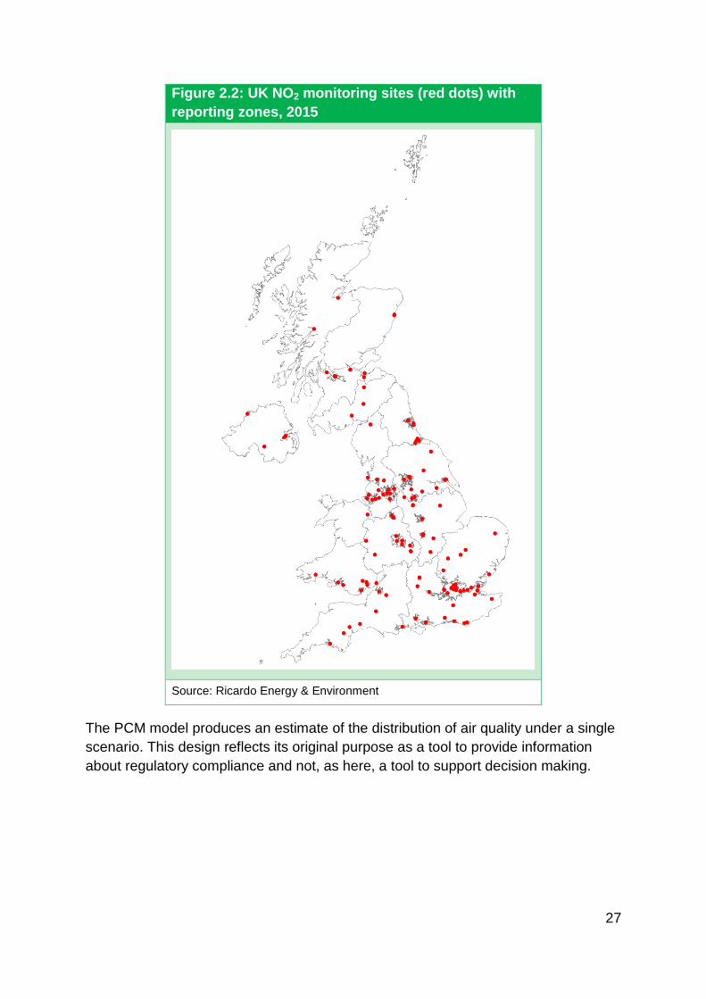
Figure 2.2: UK NO2 monitoring sites (red dots) with
reporting zones, 2015
Source: Ricardo Energy & Environment
The PCM model produces an estimate of the distribution of air quality under a single
scenario. This design reflects its original purpose as a tool to provide information
about regulatory compliance and not, as here, a tool to support decision making.

28
However, the Streamlined Pollution Climate Mapping (SL-PCM)27 model, developed
from the full PCM model, may be used to model NO2 annual mean concentrations for
the same ~9,000 urban major roads under a number of different scenarios. The SL-
PCM model is a simplified version of the full PCM model and as a result has a
substantially reduced analysis time. These faster analysis times are possible since
the SL-PCM relies on information previously prepared for and by the full PCM model
and does not require dispersion modelling for each scenario. This makes it practical
to use the SL-PCM model outputs to investigate the sensitivity of the modelled
concentrations to different policy interventions and transport solutions. While the SL-
PCM model only calculates the impacts on concentrations of NO2 as a result of
changes in road traffic, it also contains estimates of background concentration levels
and does not allow the modelled concentrations to fall below these values. See
Annex A for quality assurance information regarding the SL-PCM model.
The effects that different policy options are expected to have on the number, type28,
size, age, type of usage and distribution of vehicles are then included within this
projection using the SL-PCM model, to arrive at an estimate of the effects of
particular policy scenarios29.
The UK is divided into 43 areas or “reporting zones” for air quality reporting. There
are two types of reporting zone: 28 agglomeration zones (large urban areas) and 15
non-agglomeration zones (Fig. 1.3). Compliance is assessed against an annual
mean concentration of 40μg/m3 and 1-hourly average concentration of 200μg/m3,
with 18 permitted exceedances of the latter each year. The annual assessment uses
information from the UK national monitoring networks and the results of the
modelling assessment for that year.
The final air quality compliance statement for each pollutant in each zone is derived
from a combination of measured and modelled concentrations. The assessment of
compliance for each zone is based on the highest concentration of the modelling and
measurements in each zone.
27 Ricardo Energy & Environment, ‘Streamlined PCM Technical Report’, Report for Department for
Environment, Food & Rural Affairs (project AQ0959), 2015 <https://uk-
air.defra.gov.uk/assets/documents/reports/cat09/1511260938_AQ0959_Streamlined_PCM_Technical
_Report_(Nov_2015).pdf>.
28 European Commission, Transport Emissions: Air pollutants from road transports
<http://ec.europa.eu/environment/air/transport/road.htm>.
29 Note that the latest available SL-PCM model in March 2017 uses projections from 2013. An
updated SL-PCM model based on projections from 2015 (and fully consistent with the latest PCM
modelling) is under development and will be used for analysis published in the final Plan.

29
Although modelling projections may predict that zones will exceed the limit in a
certain future year (year n), the compliance status only becomes official once both
the monitoring and historical modelling assessment are combined and the overall
assessment is completed (in year n+1). Hence, the latest compliance assessment,
published in September 2016, is for 2015.
2.2 Results
2.2.1 Model validation
The relationship between the results from modelling air quality and those from
independent measuring sites (Fig. 2.3) shows that the level of accuracy of modelling
was normally within ±30% of the measured value and there was no evidence of
significant non-linearity in the modelled data. This suggests that modelled data has
validity as a method for estimating actual NO2 concentrations but with the caveat that
estimates based on models will have additional uncertainty.
Figure 2.3: The relationship between modelled NO2 concentration and the
NO2 concentrations measured in 2013 using the wider national network (a)
and validation sites within the local authority network (b)
(a)
Based on
measurement
data from
national
background
monitoring sites.
R2 = 0.88;
number of data
points = 71.

30
(b)
Based on
measurement
data from
independent
verification sites.
R2 = 0.71;
number of data
points = 57.
Note: R2 provides a measure of how well observed outcomes are replicated by a model,
based on the proportion of total variation of outcomes explained by the model. Values
range from 0 to 1, with 1 representing a perfect correlation.
2.2.2 Compliance
Past compliance data and results for the UK can be found online30 31. As well as
these official reports on air quality data, information is made available to the public
via annual ‘Air Pollution in the UK’ reports32.
Table 2.4 summarises the NO2 assessment in the latest version of this report and
provides a comparison with the results of the assessments carried out in previous
years since 2008 when the limits came into force.
30 EIONET Central Data Repository, Information on the attainment of environmental objectives (Article
12) <http://cdr.eionet.europa.eu/gb/eu/aqd/g/>.
31 EIONET Central Data Repository, Annual report (questionnaire) on air quality (2004/461/EC)
<http://cdr.eionet.europa.eu/gb/eu/annualair>.
32 Department for Environment, Food & Rural Affairs, Air Pollution in the UK report <https://uk-
air.defra.gov.uk/library/annualreport/>.

31
Recent revisions to COPERT emission factors were discussed in Section 2.1. These
changes have been incorporated into the revised 2015 base year compliance
modelling of NO2 presented in the draft Plan. As there are no requirements to back-
correct previous assessments, historical compliance results prior to 2015 will not be
updated retrospectively.
2.2.3 Air quality projections
Projections based on the historical 2013 assessment estimated the annual average
NO2 concentrations across the UK up until 2030 (Table 2.5). While the 2013
assessment itself has not been retrospectively updated in light of the revised
COPERT emission factors, the corresponding projections have been updated to
reflect the latest estimates data. These projections represent what may happen if no
further action is taken to control air quality. These projections include the impact of
policy interventions that have already been taken or for which there is a firm
commitment to implement33. They show that, in the absence of further interventions,
all regions apart from one (London) will be compliant by 2027. This is because
continual vehicle fleet turnover means older more polluting vehicles are replaced
with newer cleaner vehicles.
33 New policies set out in the 2015 Air Quality Plan, including Clean Air Zones in five English cities,
have not been included in the baseline projections because they are expected to materially change as
a result of the new Plan.
Table 2.4: Number of non-compliant UK reporting zones for NO2 concentration
limit values for 1-hourly and annual assessments, 2008-2015
Limit value 2008 2009 2010 2011 2012 2013 2014 2015
NO2 1-hourI 3 2 3 3 2 1 2 2
NO2 AnnualII 40 40 40 35 34 31 30 37
I An hourly average concentration of 200μg/m
3, with 18 permitted exceedances each year. No
modelling for 1-hour LV.
II Between four and eight additional zones exceeded the annual mean NO2 limit value each year from
2011-14 but were covered by time extensions and within the limit value plus margin of tolerance,
therefore compliant. 2015 was the first year with no time extensions for NO2: this is the reason for the
apparent increase in zones exceeding between 2014 and 2015.

32
Table 2.5: Number of zones projected to be non-compliant with the limit
value for NO2 assuming no additional policy interventions to those
currently in place
Year 2017 2018 2019 2020 2021 2022 2023
No. of zones 37 36 34 31 22 18 9
Year 2024 2025 2026 2027 2028 2029 2030
No. of zones 3 3 3 1 1 1 1
Under the previous projections published in 201534, 8 zones were expected to
remain non-compliant by 2020 without further action. These latest projections (Table
2.5) indicate that this has now increased to 31 zones. This difference is the result of
developments in the evidence base, most notably around increased NOx emissions
from Euro 5 LGVs, Euro 6 LGVs and Euro 6 diesel cars.
Figure 2.6 demonstrates that roads projected to exceed the NO2 limit value occur in
different orientations. In some situations, these roads are contained within an urban
centre where it might be feasible to implement a Clean Air Zone to control emissions
(Fig. 2.6a). There are also instances where an individual road outside an urban
centre (e.g. a bypass, Fig. 2.6b) is projected to exceed the limit value, where a Clean
Air Zone would not be appropriate, and an alternative solution is required.
34 Department for Environment, Food & Rural Affairs, Air Quality in the UK: plan to reduce nitrogen dioxide
emissions, 2015 <https://www.gov.uk/government/publications/air-quality-in-the-uk-plan-to-reduce-nitrogen-
dioxide-emissions>.

33
Figure 2.6: Examples of orientation of roadside exceedances; showing
exceedances contained within an urban centre (a), and exceedances located
on routes into the city and on a bypass (b)
Note: The roads are coloured according to the NO2 concentration in µg/m3 (see scale to the left).
AQMA = Air Quality Management Area; LA boundary = local authority boundary.
Section 9 describes in more detail the work that is underway to provide updated
PCM modelling in time for the final Plan.
2.3 Discussion
The PCM and SL-PCM models combine to provide a picture of how air pollution may
change in future. The accuracy of the models means that there is a need to consider
that the estimates of future air pollution will contain a level of uncertainty in addition
to uncertainty associated with the expected number and distribution of sources and
their characteristics. For example, if vehicle technology does not deliver the
anticipated NOx emission reductions then the number of zones not compliant with air
quality standards for NO2 in future years would be greater than the numbers shown
Table 2.5.

34
3. Option assessment
3.1 Introduction
Given the scale of the challenge set out in Section 2, this section looks at what policy
options might be undertaken to improve air quality. In particular, it describes the
process by which the options considered in the draft Plan were identified, as well as
how the different options have been assessed against each other. Following this, the
results of a high-level assessment of the theoretical maximum technical potential of
the proposed measures is given. Exploration of the theoretical maximum technical
potential acts as a catalyst to explore the scope of options that could feasibly be
implemented as a measure to control air quality.
While policy related to air quality in the UK is devolved, air quality evidence is not. In
particular, for compliance reporting a single assessment of air quality across the UK
is made. Therefore, during the development of this technical report the modelling of
different options has been conducted on a UK wide basis. Ultimately, the UK
Government, the Scottish Government, the Welsh Government and the Department
of Agriculture, Environment and Rural Affairs in Northern Ireland will each decide on
the policies to introduce for exceedances in their areas.
The selection and assessment of options to improve air quality has been conducted
based on the central appraisal guidance ‘Public Sector Business Cases Using the
Five Case Model (2013)’35. It has been necessary to adapt the approach for this
consultation to address two particular challenges. First, the analysis needed to be
completed in less than five months to allow the consultation to be published by the
court deadline. Second, the final Plan is not intended to complete all the stages of
the five case model through to implementation and evaluation.
A three-stage method has been developed to enable these challenges to be
addressed (Fig. 3.1).
35 HM Treasury, The Green Book: appraisal and evaluation in central government,
<https://www.gov.uk/government/publications/the-green-book-appraisal-and-evaluation-in-central-governent>.

35
Figure 3.1: A three-stage method adapted from the ‘Public Sector Business
Cases Using the Five Case Model’ to suit the plan-specific challenges
Section 3.2 and Section 3.3 address how stages 1 and 2 were conducted
respectively, whilst the details of how stage 3 will be conducted, following the
consultation, is described in Section 9.2.
Stage 3: Full analysis of plan
Package development National air quality assessment
Stage 2: Short listed option analysis
Air quality change Delivery timetable Deliverability
Stage 1: Identification of long list options
Technical options Behavioural change

36
3.2 Identification of options for emission reduction
A range of techniques were used to identify a long list of different options to improve
air quality in the first stage of the approach to identifying and assessing potential
options for reducing emissions of NOx (Fig. 3.2).
Figure 3.2: A process flow diagram displaying the range of techniques
used to identify the long list of air quality improvement options

37
3.2.1 Sources of NOx
The compliance assessments and baseline projections described in Section 2 show
when and where modelling indicates there are nitrogen dioxide (NO2) exceedances
in the UK. To reduce concentrations of NO2, it is important to understand where it
comes from so that the sources can be tackled. This is done by looking at emissions
of nitrogen oxides (NOx) made up of NO2 and nitric oxide (NO), because NO can be
oxidised into NO2 in the atmosphere.
One output of the PCM model is detailed information on the sources of NOx (source
apportionment) that go on to influence annual mean NO2 concentrations, which
helps target options for improvement. The source apportionment of NOx emissions
can be divided into regional, urban, and local scales. The regional scale includes
within country, trans-boundary36, and shipping sources; the urban scale includes
sectors such as road traffic, industry, and domestic; and the local scale includes a
split into different vehicle classes, such as cars, buses, and HGVs.
The national average categorisation of NOx coming from different sources for the UK
in 2015 was shown in Figure 1.2. Apportionment of NOx to sources is used as a
proxy for the apportionment of NO2 to sources. This allocation of the average annual
NO2 concentration to different sources is complicated by the fact that NO2 can be
derived indirectly from some sources because of the oxidation of the NO portion of
NOx. This complexity is set out in more detail in Box 3.3.
The analysis of sources of NOx emissions shows that the road transport sector is the
single largest contributor to the NO2 challenge, accounting for some 80% of NOx
emissions in 2015 at the roadside. Thus, it is evident that tackling NO2 exceedances
requires addressing road transport emissions. Actions to tackle other sources are
summarised in the draft UK overview document.
36 Including pollution transported in to a region from another region and also from another country to
the UK.

38
Box 3.3: Relationship between NOx emissions and NO2 concentrations
The relationship between NOx emissions and NO2 concentrations is complex. For a given
reduction in NOx concentration, the corresponding reduction in NO2 is dependent upon the
initial NOx concentration, as illustrated in the figure below. Factors such as the presence of
other pollutants, temperature and wind speed can also have an impact.
This can be demonstrated by observing points A and B, which reside in locations of low and
high pollution concentrations respectively. A reduction of 50µg/m3 NOx results in a reduction
of over 30µg/m3 NO2 for locations of low pollution concentrations. In contrast, the same
reduction in NOx concentration at a second more highly polluted location only results in a
reduction of just under 16µg/m3 in NO2 concentration.
As this shows, where the starting concentration of NO2 is already high, a higher reduction in
NOx will be required to deliver the same reduction in NO2 concentrations. The complexity is
further increased by the variation in primary NO2 emissions from one location to another,
meaning the curves can be different for different locations.
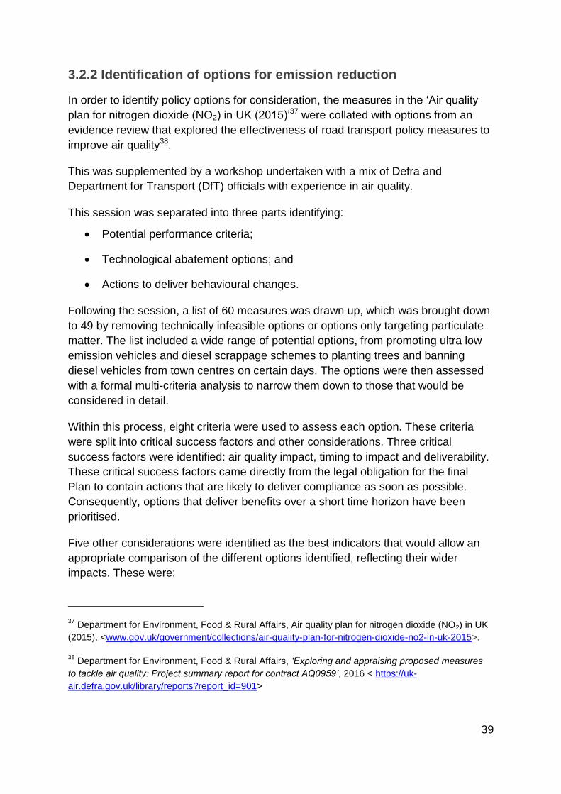
39
3.2.2 Identification of options for emission reduction
In order to identify policy options for consideration, the measures in the ‘Air quality
plan for nitrogen dioxide (NO2) in UK (2015)’37 were collated with options from an
evidence review that explored the effectiveness of road transport policy measures to
improve air quality38.
This was supplemented by a workshop undertaken with a mix of Defra and
Department for Transport (DfT) officials with experience in air quality.
This session was separated into three parts identifying:
Potential performance criteria;
Technological abatement options; and
Actions to deliver behavioural changes.
Following the session, a list of 60 measures was drawn up, which was brought down
to 49 by removing technically infeasible options or options only targeting particulate
matter. The list included a wide range of potential options, from promoting ultra low
emission vehicles and diesel scrappage schemes to planting trees and banning
diesel vehicles from town centres on certain days. The options were then assessed
with a formal multi-criteria analysis to narrow them down to those that would be
considered in detail.
Within this process, eight criteria were used to assess each option. These criteria
were split into critical success factors and other considerations. Three critical
success factors were identified: air quality impact, timing to impact and deliverability.
These critical success factors came directly from the legal obligation for the final
Plan to contain actions that are likely to deliver compliance as soon as possible.
Consequently, options that deliver benefits over a short time horizon have been
prioritised.
Five other considerations were identified as the best indicators that would allow an
appropriate comparison of the different options identified, reflecting their wider
impacts. These were:
37 Department for Environment, Food & Rural Affairs, Air quality plan for nitrogen dioxide (NO2) in UK
(2015), <www.gov.uk/government/collections/air-quality-plan-for-nitrogen-dioxide-no2-in-uk-2015>.
38 Department for Environment, Food & Rural Affairs, ‘Exploring and appraising proposed measures
to tackle air quality: Project summary report for contract AQ0959’, 2016 < https://uk-
air.defra.gov.uk/library/reports?report_id=901>

40
The cost incurred by central Government in implementing the option;
The costs and benefits of wider societal impacts associated with the option;
Changes in the level of greenhouse gas (GHG) emissions as a result of the
implementation of the option;
The extent to which the option aligns with wider Government objectives (the
strategic fit); and
The potential impact of the option in supporting future economic growth.
The options were assessed against these criteria by members of the Defra/DfT Joint
Air Quality Unit, using their working understanding and available evidence. The
assessment scores were subsequently weighted, with each critical success factor
given triple the weighting of the other factors. The results of this exercise were then
tested with key individuals in DfT and Defra.
Table 3.4 is a shortlist of policies developed from the most suitable options in the
analysis.The shortlist was derived based on the scores in Table 3.5, with additional
options added for completeness, and some policies merged where they work well
together. More detail on each option in Table 3.4, including a full analysis of their air
quality impact and costs and benefits follows in Sections 4, 5 and 6.

41
Table 3.4: Short-listed options to reduce NOx emissions
Option Description
Clean Air Zones
(CAZs)39
A geographically defined area bringing together immediate action to
improve air quality. CAZs can include a charging element for vehicles
that enter that do not meet the required standard.
Clean Air Fund
(CAF)
A clean air fund could provide financial support for Local Authorities
to fund local measures such as implementing sustainable transport
strategies.
Scrappage National targeted car and van scrappage scheme that would
incentivise the move to a cleaner fleet; increasing turnover by
targeting the removal of the oldest and dirtiest vehicles.
Retrofit Providing national support for the installation and operation of
abatement equipment on existing buses, taxis, and heavy goods
vehicles.
Ultra Low Emission
Vehicles (ULEV)
Providing additional support to purchasers of Ultra Low Emission
Vehicles (ULEV).
Tax Adjusting vehicle excise duty, fuel duty and company car tax to
create incentives towards less polluting vehicles. This is a reserved
matter for the Treasury and will be assessed independently of this
exercise.
Speed limits Reducing speed limits on motorway links that are not complying with
the legal air quality obligations.
Government buying
standards for
transport (GBS-T)
Expanding the use of GBS-T40 to include emissions of NOx and PM.
Vehicle labelling Reflect air quality performance of vehicles on their labelling to allow
consumers to make decisions that are more informed.
Influencing driving
style
Encouraging less polluting driving styles through reducing aggressive
driving.
Government
independent
assurance
Establishing a body to review and support the delivery of air quality
improvements. This is not a measure that would in itself deliver air
quality improvements and so is not analysed in this report.
39 Department for Environment, Food & Rural Affairs, Implementation of Clean Air Zones in England,
<www.gov.uk/government/consultations/implementation-of-clean-air-zones-in-england>.
40 Department for Environment, Food & Rural Affairs, Sustainable procurement: the Government
Buying Standards (GBS), <www.gov.uk/government/collections/sustainable-procurement-the-
government-buying-standards-gbs>.

42
Table 3.5: Scores from a multi-criteria analysis of the relative suitability of different emission reduction options, options were
rated on a range from 1-3 and key criteria weighted by a factor of 3, a higher score indicates a more positive assessment
Emission reduction option
Key criteria Secondary criteria
Total scores Timing
Impact
on NOx
Deliver-
ability
Cost to
Gov.
Cost to
consumer
Strategic
fit
Economic
growth
GHG
emissions
Expand Clean Air Zones 9 9 9 2 1 3 1 3 37
Expanded retrofit programme 9 6 6 2 3 2 3 3 34
Drive down shorter journeys 9 3 9 3 3 2 2 3 34
Reduce speed limits 9 6 9 3 1 1 1 3 33
Promote ultra-low emission vehicles 9 3 9 1 3 3 2 3 33
Carpool lanes 9 3 9 2 3 2 1 3 32
Promote alternative fuels 9 3 9 3 1 3 2 2 32
Promote better driving 9 3 9 3 2 2 1 3 32
Ban dirtiest cars on high pollution days 9 6 6 3 1 2 1 3 31
Wider policies to discourage diesel purchase 9 3 9 3 2 1 2 2 31
Reduce Government’s use of diesel vehicles 9 3 9 3 3 2 1 1 31
Use VEDii and/or CCT
iii to promote low NOx vehicles 6 6 9 3 1 3 1 1 30
Introduce vehicle labelling system 6 3 6 3 1 3 1 2 25
I Vehicle Excise Duty.
II Company Car Tax.

43
3.3 Impact assessment methods
This section describes the methods used to assess the impacts to the UK of the
shortlisted options in Table 3.4. As explained in Section 3.1, the assessment covers
all of the UK even though ultimately different policy decisions may be made for
England, Scotland, Wales, and Northern Ireland. An assessment of these options
was conducted according to the process laid out in Figure 3.6.
In addition to reducing NO2 concentrations, the measures taken will have a range of
other impacts. The assessment therefore attempts to reflect these impacts through
cost-benefit analysis. It is not possible to assess all the impacts and so this analysis
focused on the most significant direct impacts as required by the best practice
appraisal guidance (the Green Book41). Uncertainties inherent in all appraisals of
future events mean there are risks to delivery of the assessed impacts. How these
are dealt with and the steps taken to ensure that options are continually assessed
against their desired affects are discussed in Sections 8 and 9.
The options were assessed at this stage against the two quantifiable critical success
factors (CSFs) in Section 3.2.2: the scale of the improvement (the concentration
reduction) and the time until the improvement begins to be realised. These critical
success factors were directly derived from the legal obligation for the final Plan to
contain measures that are likely to deliver compliance as soon as possible;
consequently, options offering the highest abatement in the shortest time were seen
to be most desirable.
Following this, a cost-benefit analysis was undertaken to consider the wider
implications of the measures over a ten-year appraisal period. The monetised
impacts include the health benefits from reduced exposure to NO2, impacts from
changes to greenhouse gas emissions, cost to Government and cost to the public. A
ten-year appraisal period for assessment was chosen as this was considered the
time horizon over which most of the impacts of options were expected to be
observed, whilst being consistent with the Green Book guidance. The impacts were
then discounted42 and summed to calculate the net present value (NPV) of the
options. Throughout this analysis, 2017 was used as the price base year as well as
41
HM Treasury, The Green Book: appraisal and evaluation in central government,
<https://www.gov.uk/government/publications/the-green-book-appraisal-and-evaluation-in-central-
governent>.
42 See Section 3.3.3 for more information.

44
the present value base year. As a result, the NPV indicates a policy options
monetised net value in terms of 2017 prices.
The starting year of the ten-year appraisal period for each policy option was different
depending on the specific nature of the option. The appraisal period of each option
begins in the year when the first costs associated with the option are assumed to be
incurred (e.g. setup and implementation costs). However, air quality impacts may
only be exhibited after the start of the appraisal period for some options due to the
setup time involved.
Finally, the strategic fit was assessed to understand how well the policy is likely to fit
with national priorities and other Government policies. This considered what impact
the options would have on different demographic groups within the population, and
the impacts on economic growth. Figure 3.6 provides a visual representation of the
option assessment process.
For the consultation, the most significant impacts have been assessed and, as far as
possible, quantified. At this stage, five such impacts have been assessed:
Health benefits – reflecting the reduced cost of health problems linked to NO2
Social cost – reflecting the costs of the given action to society
Benefits from traffic flow improvements – monetised using the value of time
saving
Government cost – including implementation and setup costs
Change in greenhouse gas emissions – valued using the social cost of
carbon.
For the final Plan, a cost-benefit analysis of the impacts of the proposal will be
undertaken to provide a transparent assessment of the impacts of the final package
of measures. More detail on how analysis will be developed for the final Plan is set
out in Section 9.1.
The remainder of this section describes how each of the criteria set out above have
been assessed.

45
Figure 3.6: A flowchart showing the process for assessing the net impacts of
different emission reduction options.

46
3.3.1 Interim year air quality assessment
For this draft plan, full modelling of air quality impacts is only available for the years
2020, 2025, and 2030. In order to assess the impact of the policy options on air
quality in the interim years, the data from these three modelling assessments has
been interpolated. For policies that start prior to 2020, the 2020 SL-PCM modelling
outputs have been interpolated with the 2015 full PCM modelling outputs.
Interpolation is a method of estimating values between a known set of data points. A
linear interpolation method between the two closest modelled data points has been
employed for this report (i.e. for the 2023 baseline, a linear interpolation between
2020 and 2025 baseline outputs has been calculated).
Alternative interpolation methodologies, including a linear function, a square
polynomial function, and a cubic polynomial function, have been compared to the
linear interpolation methodology (Annex H) in order to determine which produced the
most accurate results. The analysis concluded that the interpolation methodology
used in this report produced results that were extremely close to actual projected
values (with a correlation coefficient of 0.998). It also found the method produced
slightly conservative results in the years 2020-2025. In this period, the interpolated
values were higher than the actual values, meaning that areas were more likely to be
considered non-compliant with NO2 limits. Therefore, this methodology would lead to
a slight overestimation of the expected number of NO2 limit exceedances in these
years.
It should be noted that interpolating the concentration values in interim years will not
be necessary for the final Plan because the SL-PCM model will be updated to
generate additional outputs for these years (see Section 9.1).
3.3.2 Health impacts valuation
Much of the evidence linking health impacts with long-term average NO2
concentrations has been gathered using observational epidemiological studies.
These studies use statistical methods to identify associations between outcomes,
such as mortality or ill health, with external factors, such as modelled or measured
pollutants levels, whilst taking into account other variables such as sex and age.
Observational epidemiological studies are only able to provide evidence of effects
based on a statistical relationship between risk factors and health outcomes.
Concentrations of NO2 and some other pollutants such as PM2.5 are closely
correlated because they are emitted from the same sources (for example traffic).
Although the statistical procedures attempt to disaggregate the effects of the
individual pollutants, this correlation means that some of the statistical association
found with NO2 may represent effects caused by other correlated pollutants. There

47
is, therefore, uncertainty in the extent to which the association between long-term
average concentrations of NO2 and mortality is causal. The Committee on the
Medical Effects of Air Pollutants (COMEAP) has noted that:
"…it is possible that, to some extent, NO2 acts as a marker of the effects of
other traffic-related pollutants…"
COMEAP considered the evidence linking long-term average NO2 concentrations
with effects on mortality, with a view to recommending methods for quantifying this
association and estimating the mortality effect in the UK. In their advice to Defra in
July 201543 they recommended that a coefficient of 1.025 (95 percent confidence
interval 1.01–1.04) per 10µg/m3 NO2 could be used in cost-benefit analysis to reflect
associations between long-term average concentrations of NO2 and all-cause
mortality. This means that for every 10µg/m3 increase or decrease in concentrations,
there will be a 1% to 4% increase or decrease in mortality. For the central analysis in
this technical report, the central 2.5% coefficient has been applied. In order to
ascertain how varying the coefficient may impact mortality, the 1% and 4%
sensitivities have been tested and presented in Section 8.3.
COMEAP explained that the uncertainty in applying a coefficient to assess the health
benefit of measures to reducing NO2 would depend on the extent to which the policy
option is specific to NO2, or also reduces concentrations of other co-emitted
pollutants. There is likely to be more uncertainty when the option is specific for a
reduction in NO2, compared to when an intervention aims to reduce the whole
mixture of pollutants. None of the interventions assessed in this report are expected
to increase emissions of other air pollutants.
In December 2015, COMEAP published an interim statement explaining that there
was potentially considerable overlap between the increased mortality risks found to
be associated with concentrations of NO2 and PM2.544. COMEAP continues to
develop their advice on this as the scientific evidence develops. The uncertainty
surrounding these effects can have potentially large impacts on the cost-benefit
assessments.
Defra has calculated interim NOx damage costs by applying the coefficients
recommended by COMEAP to all types of intervention that reduce NOx emissions.
43 Appended to Committee on the Medical Effects of Air Pollutants, ‘Interim statement on quantifying
the association of long-term average concentrations of nitrogen dioxide and mortality’, 2015
<www.gov.uk/government/uploads/system/uploads/attachment_data/file/485373/COMEAP_NO2_Mor
tality_Interim_Statement.pdf>.
44 Ibid.
48
Damage costs are a simple way to value changes in air pollution. They estimate the
cost to society of a change in emissions of different pollutants. Damage costs are
provided by pollutant, source, and location45; health outcomes have been valued
using these in accordance with Defra guidance46. In due course, this guidance will be
updated as new evidence and scientific advice becomes available.
In order to monetise the health impacts arising from a change in NO2 concentrations,
the location-specific damage costs were multiplied by the total tonnage change in
emissions in that area. These were then totalled for each year to provide an
overview for the whole UK.
As laid out in Section 2 the tonnage change in NOx emissions for each of the short-
listed policy options has been calculated using the PCM and Streamlined PCM
models. The health impacts from these changes in NOx emissions have been valued
using NOx damage costs for all of the options assessed in this report. For the
charging CAZ option, the damage costs used are based upon the proportion of
emissions falling within each type of urban location: transport central London,
transport inner London, transport outer London, inner conurbation, urban big and
urban large. For the other policies assessed in this report, the transport average
damage cost is used as these policies do not target a certain geographic area47.
These total annual values are then uplifted by 2% per annum, from the base year of
2015 in line with best practice (Green Book) guidance48, to take into account the
assumption that the willingness to pay for improvements in health will rise in line with
economic growth.
45 Further information on damage costs is available at <https://www.gov.uk/guidance/air-quality-
economic-analysis>.
46 Department for Environment, Food & Rural Affairs, Air quality: economic analysis,
<https://www.gov.uk/guidance/air-quality-economic-analysis#damage-costs-approach>.
47 The geographical definitions used for damage costs are based on the definitions provided for
transport modelling. Department for Transport's transport appraisal guidance (WebTAG) provides
more information on each of these areas. This guidance is available at
<www.gov.uk/guidance/transport-analysis-guidance-webtag>.
48 Department for Environment, Food & Rural Affairs, ‘Valuing impacts on air quality: Supplementary
Green Book guidance’, <www.gov.uk/government/publications/green-book-supplementary-guidance-
air-quality>.

49
3.3.3 Other societal impacts valuation
Where possible, each of the shortlisted measures has been assessed for any other
significant societal costs and benefits using consistent valuation approaches. For
example, the benefits of reducing congestion in CAZs or the costs of increased
journey times by reducing speed limits.
The most sophisticated of these valuation processes is the Fleet Adjustment Model
(FAM), which is used for assessing charging CAZs. Further, the Scrappage/Retrofit
Model, which uses many of the same inputs and valuations as the FAM, has been
used to assess both the scrappage and retrofit proposals. Finally, other measures
have been assessed using simpler bespoke, but consistent, approaches that are
described alongside the results in Sections 5 and 6.
There follows brief descriptions of the main two models: the FAM and
Scrappage/Retrofit Model.
Fleet Adjustment Model
The FAM quantifies the societal costs and benefits associated with changes in the
UK’s vehicle fleet. This fleet change may be triggered by many different policies, but
the model has been used here for the charging CAZ assessment.
The FAM was developed and published49 alongside the 2015 UK Air Quality Plan for
tackling nitrogen dioxide, and the latest technical documentation is attached in
Annex B. Figure 3.7 outlines a brief overview of the sequential stages within this
model.
49 See Annex D of
<www.gov.uk/government/uploads/system/uploads/attachment_data/file/492901/aq-plan-2015-
technical-report.pdf>.

50
Figure 3.7: A flow chart to illustrate the process by which the Fleet
Adjustment Model evaluates an option
In the first stage, the baseline scenario establishes the vehicle fleet in different years
before the implementation of any policy adjustments. The baseline is established via
two key inputs:
the fleet composition (number of vehicles by age and vehicle type - buses,
coaches, taxis, HGVs, LGVs and cars); and
the number of vehicle kilometres driven by each type of vehicle, inside and
outside of the proposed CAZ and their location.
The second stage introduces measures that have an impact on the vehicle fleet. It
models individual owners’ specific responses to the options introduced. The
responses will depend on the costs of different options available and the specific
nature of the option. In relation to CAZs, some vehicle owners may choose to
upgrade vehicles or avoid the restricted zone, triggering changes in the fleet
composition and to the proportion of time older vehicles spend driving in different
locations.
The third stage then quantifies and values the main societal impacts of the changes
in fleet relative to the baseline. These impacts, in order of significance, include:
st stage
stablish
baseline and
inputs
nd stage
Change in
fleet due to
polic
rd stage
Benefits mission reduction
C reduction
rd stage
Costs Consumer surplus loss
oss of asset value
mplementation cost
et Present
alue (Benefits –
Costs

51
Health benefits:
The CAZ option will lead to vehicle owners changing their behaviour, for example
by upgrading to a cleaner vehicle, cancelling a journey, avoiding zones or
redeploying vehicles to less polluted areas. These behavioural responses will
result in overall reductions in vehicle trips and in the replacement of older dirtier
vehicles with newer less polluting ones, both of which result in lower emissions
and therefore benefits to health.
Social costs:
Owners of vehicles below the required Euro standard will have to change their
behaviour in one of the ways listed above. The new action is favoured less than
their baseline behaviour (otherwise they would have been doing it already);
hence these vehicle owners will incur an additional cost, termed welfare loss in
economics.
Traffic flow improvements:
Alongside changes in the fleet, additional impacts may be felt from changes in
the behaviour of vehicle owners. Vehicle owners who choose not to make their
journey will be reducing the number of vehicles on roads within each of the
CAZs. While it is assumed that business journeys using non-compliant vehicles
will be replaced by equivalent businesses with a compliant vehicle, affected
private car journeys are assumed not to be replaced. Consequently, less traffic
on roads would lead to faster journey times for other users.
Government costs:
There will be both set up and ongoing costs to deliver improvements in air
quality. Such costs could include scoping studies, infrastructure including
installation costs and IT equipment and ongoing running costs such as
communication, enforcement and staff costs.
Change in greenhouse gas emissions:
Modelling results show that overall charging CAZs are likely to reduce CO2
emissions slightly. Reductions in the level of CO2 emissions have been valued
for vehicle scrappage and foregone trips. Where owners replace vehicles with a
compliant vehicle a CO2 emission saving is not expected, as the vehicle is sold to
another user who will continue to use it (unless it is scrapped). Where vehicles

52
are scrapped there will be a CO2 saving. These savings have been valued using
an average CO2 non-traded central carbon price for the appraisal50.
Finally, all the impacts are discounted and the total costs are subtracted from the
total benefits providing a net present value (NPV).
Scrappage / Retrofit Model
This model has been developed from the FAM to provide an assessment of the
impacts of a scrappage and retrofit scheme. It allows the assessment of different
potential scrappage scheme policy options around the type of replacement vehicle
and the levels of grant required to ensure a given level of take up. This model has
also been used to assess different potential retrofit policy options (further detail on
the assumptions is provided in Section 8). The scrappage model is comprised of four
key stages, which have been outlined below.
Stage one establishes the baseline vehicle fleet in different years prior to any policy
adjustments. The key inputs are: the national fleet composition by vehicle type, Euro
standard, fuel type, mileage, and average NOx and CO2 emissions for vehicle types
by Euro standard, and fuel type. These inputs are consistent with the inputs in the
FAM already outlined.
Stage two introduces the policy option and estimates the emission savings
associated with the policy measure. Specifically, it estimates emissions of new
vehicles purchased from a scrappage scheme, and compares these to vehicles in
the baseline. The key simplifying assumption in the model is that the average
mileage of the replacement (or retrofitted) vehicle and the vehicle that is scrapped
(or retrofitted) is equivalent.
In stage three, the model estimates the number of vehicles that are expected to be
scrapped. The estimated number of vehicles scrapped and replaced with
conventional vehicles is estimated based on the residual value of vehicles. Where
the value of the scrappage scheme payment is higher than the residual (second
hand) value of vehicles, it is assumed that these vehicles are scrapped. For a policy
of scrappage to Ultra Low Emission Vehicles, a top down estimate has been
produced based on benchmarking using similar schemes and existing evidence. The
adoption of retrofit has been estimated based on assessments of market capacity for
50 Table 3: Carbon prices and sensitivities 2010-2100 for appraisal, 2015 £/tCO2e
<www.gov.uk/government/uploads/system/uploads/attachment_data/file/483282/Data_tables_1-
20_supporting_the_toolkit_and_the_guidance.xlsx>.

53
retrofit. It is assumed that the offer of free retrofit will incentivise its uptake,
particularly if there are access restrictions on non-compliant vehicles.
Finally, stage four quantifies and values the main societal impacts of the changes in
fleet relative to the baseline. At this stage the most significant impacts that have
been assessed and as far as possible quantified, are:
Health benefits – reflecting the cost of health problems linked to NO2;
Welfare cost – reflecting the lost residual asset value to society, operating
cost savings to the consumer and any deadweight loss;
Government cost – including the level of compensation for the grants;
Change in greenhouse gas emissions – valued using the social cost of
carbon.
Finally, all the impacts are then discounted and total costs are subtracted from the
total benefits providing a net present value (NPV).
3.3.4 Net present value and discounting
The net present value (NPV) of an option is calculated by summing the present
values of the costs and benefits attributed to the option. Present values are obtained
by discounting costs and benefits over time to account for people’s time preferences.
People tend to place a higher value on immediate impacts rather than those incurred
in the future. This is because future events are less certain and because people
expect to be financially better off in the future. In this analysis, the Treasury
recommended discount rate of 3.5% per annum has been used to calculate the
present value of the monetised costs and benefits for each option51.
The net present value provides a broad indicator of the performance of an option.
The primary advantage of the NPV is that it provides a transparent assessment of
the different policy options by using the best available evidence and a systematic
approach to the valuation of the impacts arising from the implementation of a
particular option. Positive net present values indicate that the monetised stream of
benefits of the option over the appraisal period outweigh the corresponding costs. In
51 HM Treasury, The Green Book: appraisal and evaluation in central government,
<https://www.gov.uk/government/publications/the-green-book-appraisal-and-evaluation-in-central-
governent>.

54
contrast, negative net present values highlight that the monetised cost of the option
outweighs the benefits over the appraisal period.
Given the range of uncertainties associated with the evidence used to value impacts
(see Section 8.4) it should be recognised that the net present value estimates are
only as robust as the inputs used to produce them. Thus, the values presented could
change substantially as new evidence emerges; including the potential to shift some
positive net present value estimates to negative estimates.
3.3.5 Analysis of effects among social groups
Groups in society will be affected differentially by NOx emission reduction options.
This will include how the health and financial impacts are distributed. Section 7 of
this report provides an initial summary of findings in both these areas. Specifically, it
reviews existing national-scale evidence (in the form of published articles) and
outlines the likely effect of the proposed emissions reduction options. It also provides
analysis based on information available from the National Travel Survey and other
similar sources.
Further analysis has been conducted on the financial impact of the options on
specific groups in society, such as those on lower incomes. This is based on the
emission reduction options most likely to have specific geographic impacts, as
distinct from the national picture. In particular, it focuses on charging CAZs, which
have both the greatest overall impact and most localised financial impacts. This
analysis has been carried out using both existing survey data and modelling from the
FAM (Section 3.3.3).
3.3.6 Economic growth
The impact on economic growth has been assessed qualitatively for each of the
options.
3.3.7 Quality assurance of analysis
All analysis presented in this technical report has been quality assured by other
analysts in order to check for calculation errors and to test the credibility and
appropriateness of any assumptions used. Checks have also been made on the
inputs and model runs which use the established SL-PCM and FAM models to
mitigate against any data entry errors.
For the bespoke pieces of analysis created for assessing the impacts of all except
the CAZ option, thorough checks of all calculations and assumptions have been
completed. These checks have included testing the logic of assumptions in relation
to the policy descriptions set out in this document as well as checking the model

55
formulae and coding for computational errors. The reviewers have also rerun
modelling scenarios where necessary and performed sense checks of the outputs
produced. All analysis has been checked iteratively with all changes from one
iteration to the next quality assured, and all identified issues addressed, before final
sign-off.
The FAM and SL-PCM models have both been extensively reviewed by multiple
analysts in advance of this report (see Annex A for details of SL-PCM model quality
assurance). The quality assurance process as described here focused on the
changes made to these models for the purposes of this analysis and to the inputs
used for each of the options modelled.
Another aspect of the quality assurance process has been to check that the
assumptions and data sources used are consistent across all analysis wherever
possible. These common assumptions are set out in Section 8. All options have used
the SL-PCM model to calculate the expected changes in emissions and
concentrations and the same source data has been used for each. The monetisation
of air quality and carbon impacts follow standard supplementary Green Book
appraisal guidance.
3.4 Theoretical maximum technical potential of options
Sections 4, 5 and 6 present the results of a full assessment of each policy option
conducted with the methods described so far. To help prioritise and shape the
options considered in this full analysis, first a high level assessment was undertaken
of the theoretical maximum technical potential (MTP). The MTP indicates the
maximum reduction in NO2 concentrations that could theoretically be delivered, in
the absence of real-world implementation or deliverability challenges. Therefore,
this assessment does not reflect the technical and implementation challenges
in delivering such an outcome, nor does it provide a full financial impact analysis,
but it does give an indication of the full potential of different policies to improve NO2
concentrations. To make such an assessment meaningful it also uses the same
indicative assumptions to calculate the potential costs to Government of such an
outcome.
In this way, the MTP assessment can be used to prioritise and shape the options
considered, so that a more feasible scale of implementation can be ascertained.

56
Table 3.8: Summary of results of theoretical maximum technical potential
assessment for each of the shortlisted optionsI
Option Scope
NO2 concentration
impact (mean µg/m3
reduction in 2020)II
Cost to central
Government (£m)III
Clean Air ZonesIV Targeted 11.0 600
Retrofit National 1.5 4,500
ScrappageV National 6.3 60,000
Ultra Low Emissions
Vehicles National 3.0 90,000
Speed limitsVI Targeted Up to 4.5 60
Government vehicles National 0.004 5.6
Vehicle labelling National 0.13 Negligible
Influencing driving style National 4.2 5,300
I Numbers subject to change following finalisation of analysis methods and policy design assumptions. Numbers
rounded to two significant figures.
II Air quality impacts are presented as the national mean reduction in NO2 in 2020 except for CAZs and Speed Limits,
which are targeted. 2020 is used for comparison because this is the earliest year of data in the SL-PCM model, which
has been used to estimate these impacts. Earlier impacts are modelled where policy implementation is possible before
this.
III All monetised values are net present values over a ten-year appraisal period.
IV CAZ impacts are presented only for areas where CAZs will be implemented. It has been modelled that CAZs will be
implemented covering all vehicles in 27 areas. The costs to central government reflect the costs of setting up and
running CAZs but do not capture the costs of upgrading vehicles or welfare losses for vehicle owners, which are likely
to be significant.
V National scrappage scheme assumed to scrap all pre-Euro 6 diesel cars and vans in the UK in 2019 (8 million cars
and 2 million vans, with grant levels of £6,000 and £6,500 respectively)
VI Speed limit impacts are shown just for the motorway projected to be in exceedance in 2020. These impacts cannot
be extrapolated to other roads. The impact of this measure is calculated on the assumption that traffic on failing
motorway links is travelling at the same speed as the national average (for the type of motorway). It is possible that
failing motorway links tend to be busier and more heavily congested, and that average speeds on them are lower. In
this case, a change in the speed limit may have little impact on air quality - because cars are already travelling at
speeds below the limit. Work is ongoing to improve our understanding of speeds on these links. Air quality impacts
related to speed limits are expressed as ‘up to x’ because there is uncertainty over the modelling approach in relation
to vehicle speed. Highways England’s approach would not give a reduction in NO2 concentrations or congestion
following speed limit reduction.
The assessment of the theoretical MTP is presented and explained for each policy in
greater detail in Annex C, which includes:
A brief description of the scenario considered as the maximum technical
potential;

57
An outline of key assumptions;
The projected air quality impact; and
The estimated cost to Government.
3.5 Conclusion
Source apportionment analysis shows that the road transport sector is the single
largest contributor to the NO2 challenge. Using this as a starting point, policy options
have been shortlisted for assessment using the methods described in Section 3.2.
Subsequently, to help prioritise and shape the options, an initial theoretical maximum
technical potential analysis has been conducted with the results summarised in
Table 3.8.
It is important to note that because only two impacts have been considered at the
MTP stage rather than the full range of costs and benefits, options should not be
discounted purely on the basis of this analysis. This analysis does not represent a
complete value for money assessment of these options but merely indicates options
that have the potential to deliver high air quality improvements.
The results suggest that implementation of Clean Air Zones (CAZs) is likely to be key
to achieving Government’s air quality objectives. This is based on the fact that CAZs
can potentially have significant impacts on NO2 concentrations without
disproportionate public cost; for example, the targeted nature of CAZs avoids
restricting the use of vehicles that would never operate within the areas of high
pollution. However, implementation of CAZs could potentially have notable impacts
on individuals and businesses needing to comply with the CAZ requirements. A
number of the other actions could, if scaled appropriately, help reduce the negative
impacts on those affected by CAZs. These measures include scrappage, retrofit, and
grants for Ultra Low Emission Vehicles.
Further, the investigation of CAZs revealed that not all areas with NO2 exceedances
could be effectively addressed by introducing a CAZ. For instance, exceedances
include areas of the Strategic Road Network and roads without viable alternative
routes (Fig. 2.5). National measures are likely to be needed in order to address the
air quality problems in these locations. Such measures could include speed limits on
the Strategic Road Network, Government Buying Standards for transport and
behaviour change measures such as improved driving and vehicle labelling.
The following three sections present the analysis for the shortlisted measures
following the methods outlined in Section 3.3.

58
4. Clean Air Zones
4.1 Introduction
Section 3.4 (Theoretical maximum technical potential of options) outlined eight
policies to tackle poor air quality designed without any constraints. The next three
sections of this technical report assess a feasible version of each of these options.
This step looks to reflect the real world constraints on these measures such as the
supply constraints on technologies and the process required to implement such
options.
CAZs were one of the options investigated in Section 3.4 and it is evident that this
option will be a key part of reducing NO2 concentrations. CAZs are areas where
action is focused in a particular geographical location to improve air quality and only
the use of the most polluting vehicles is discouraged.
CAZs fall into two categories:
Non-charging CAZs – These are defined geographic areas used as a focus
for action to improve air quality. This action can take a range of forms such as
facilitating the use of ULEVs and encouraging businesses to clean up their
vehicle fleets52, but does not include the use of charge based access
restrictions.
Charging CAZs – These are zones where, in addition to the above, vehicle
owners are required to pay a charge to enter or to move within the zone, if
they are driving a vehicle that does not meet the particular standard for their
type of vehicle in that zone. Charging CAZs would only be expected where
equally effective non-charging approaches are not identified.
The following section outlines the possible impact of local measures that could be
implemented as part of non-charging CAZs. The subsequent section details the
assessment of impacts that charging CAZs could have on society.
In the areas where CAZs are introduced there are further suggestions for
complementary options which would help support their implementation or to support
broader Government objectives such as aiding the transition for those least able to
manage such a change. These options have been considered in Section 5.
52 See the Clean Air Zone Framework.

59
It is also recognised that CAZs are not suitable for all the areas exceeding NO2
limits. For instance, it would not be reasonable to establish a CAZ on a single link of
motorway, or on sections of the local road network outside towns and cities.
Therefore, Section 6 reviews a range of national options that may be required in
addition to CAZs.
4.2 Local measures
There are a variety of actions that could be taken locally as part of a non-charging
CAZ that would improve air quality. Local Authorities could introduce a range of
measures such as, but not limited to:
Encouraging the uptake of Ultra Low Emission Vehicles;
Infrastructure changes;
Retrofitting the most polluting vehicles; or
Promoting public transport, cycling and walking.
These, and other, measures could be introduced in different packages, varying in
style and scope according to the local air quality problem. The effect of each project
will depend on these factors as well as characteristics of the local area, such as the
willingness of residents to change transport mode. These initiatives could have a
range of impacts in addition to improving air quality, which could range from
improved traffic flows to health improvements from additional cycling.
Due to the variability in the type of projects implemented and the associated
uncertainty in their effect on reducing NO2 concentrations a formal modelling has not
been undertaken. To illustrate the possible impacts, Box 4.1 presents a case study
looking at the effectiveness and value for money of these kinds of options. The box
draws upon evidence from a scheme targeting car usage in three urban areas,
operated by DfT.
Analysis of national level schemes for scrappage and retrofit has been presented in
Section 5. This analysis can act as a guide to the potential impacts of a scrappage or
retrofit scheme at a local level. However, as noted above the local situation will
influence their effectiveness, as will the design of specific schemes.
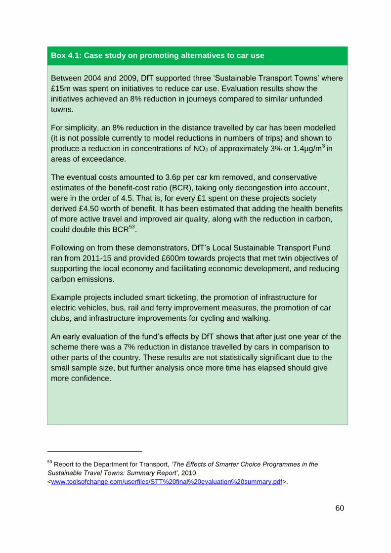
60
Box 4.1: Case study on promoting alternatives to car use
Between 2004 and 2009, DfT supported three ‘Sustainable Transport Towns’ where
£15m was spent on initiatives to reduce car use. Evaluation results show the
initiatives achieved an 8% reduction in journeys compared to similar unfunded
towns.
For simplicity, an 8% reduction in the distance travelled by car has been modelled
(it is not possible currently to model reductions in numbers of trips) and shown to
produce a reduction in concentrations of NO2 of approximately 3% or 1.4µg/m3 in
areas of exceedance.
The eventual costs amounted to 3.6p per car km removed, and conservative
estimates of the benefit-cost ratio (BCR), taking only decongestion into account,
were in the order of 4.5. That is, for every £1 spent on these projects society
derived £4.50 worth of benefit. It has been estimated that adding the health benefits
of more active travel and improved air quality, along with the reduction in carbon,
could double this BCR53.
Following on from these demonstrators, DfT’s Local Sustainable Transport Fund
ran from 2011-15 and provided £600m towards projects that met twin objectives of
supporting the local economy and facilitating economic development, and reducing
carbon emissions.
Example projects included smart ticketing, the promotion of infrastructure for
electric vehicles, bus, rail and ferry improvement measures, the promotion of car
clubs, and infrastructure improvements for cycling and walking.
An early evaluation of the fund’s effects by DfT shows that after just one year of the
scheme there was a 7% reduction in distance travelled by cars in comparison to
other parts of the country. These results are not statistically significant due to the
small sample size, but further analysis once more time has elapsed should give
more confidence.
53 Report to the Department for Transport, ‘The Effects of Smarter Choice Programmes in the
Sustainable Travel Towns: Summary Report’, 2010
<www.toolsofchange.com/userfiles/STT%20final%20evaluation%20summary.pdf>.

61
Bids of more than £5m were required to submit a proportionate appraisal of the
costs and benefits of the project. Based on the forecasts provided by 12 such
projects, receiving a total of £225m, they delivered a collective BCR of 5:154. This
conclusion demonstrates that investment in local sustainable transport projects
represents very high value for money. The value for money assessment of the
smaller bids worth less than £5m suggested that, as a package, these also
represented high value for money.
These studies show that, as well as offering air quality relief, reducing the need to
travel by car has the potential for significant decongestion benefits – and where
cycling and walking form part of the proposal significant health benefits can be
expected too.
A fund specifically targeted at local air quality improvement would expect to deliver
notable air quality benefits. These benefits cannot be quantified with the evidence
provided but the BCRs achieved by these local schemes indicate the kind of
outcomes a competitive bid scheme can achieve. They also highlight that these
kinds of funds can be successful at facilitating flexible local solutions to local
problems, which are particularly useful for the current NO2 problem.
4.3 Charging zones
4.3.1 Overview
The second category of CAZ, as set out in Section 4.1, is a charging CAZ. The key
feature of this is an access restriction, where vehicles that do not meet the standards
of the zone are required pay a charge to enter. This restriction could be introduced in
addition to a range of supporting options targeting an improvement in air quality, as
outlined in Section 4.2.
Charging CAZs are just one of a number of tools local authorities could consider
using in the development of their plans and charging is not a required element of
CAZs. Charging would only be expected where equally effective alternatives are not
identified. For this assessment of CAZs, it has been assumed that charging CAZs
are implemented at the level required to bring the affected roads into compliance.
This is purely for the modelling – Government will only mandate the measures that
54 Department for Transport, ‘Value for Money Assessment for the Local Sustainable Transport Fund’,
2014 <www.gov.uk/government/uploads/system/uploads/attachment_data/file/347894/vfm-
assessment-of-lstf.pdf>.

62
are identified by LAs as leading to compliance at the earliest point. Only the access
restriction related impacts of a charging CAZ have been modelled as the potential
effects of the supporting measures are too varied to allow a meaningful analysis.
The Clean Air Zone Framework defines four classes of access restriction based
upon the vehicle type, as set out in Table 4.2. These classes define the group of
vehicles that would face access restrictions. The sequence in which the types of
vehicle enter the different classes has been selected to target the most polluting
vehicles first. However, the class of entry restriction will need to be decided locally.
Table 4.2: Charging Clean Air Zone classes set out in the 2015 Plan for NO2
Clean Air Zone
class
Vehicles included
A Buses, coaches and taxis
B Buses, coaches, taxis and heavy goods vehicles (HGVs)
C Buses, coaches, taxis, HGVs and light goods vehicles (LGVs)
D Buses, coaches, taxis, HGVs, LGVs, cars, motorcycles and mopedsI
I The impact of including motorcycles and mopeds in CAZs have not been modelled. These
vehicles only represent a small proportion of total NOx emissions so it is not expected that they will
be included in the access restrictions for the majority of zones.
Charging CAZs are expected to lead to a change in the composition of the fleet
entering the zone, resulting in high polluting vehicles operating within the zone
largely being replaced with cleaner vehicles. This will result in less NOx emitted
within the zone. As a result of the lower emissions, concentrations of NO2 will be
reduced at both roadside and background locations.
Taking into account the minimum time it will take to implement this policy, modelling
of charging CAZs suggests that compliance could be brought forward in around 27
cities in the UK, so for the purposes of the modelling this is the number that have
been assumed. In London, the previous Mayor agreed to introduce a range of
actions including the Ultra Low Emission Zone (ULEZ), which is analogous to a
Class D Clean Air Zone, and the new Mayor has signalled his commitment to do
more than this.
In applying these actions, it is necessary to set a specific standard for each type of
vehicle. As Euro standards currently perform this function across the EU, these have
been used in setting the framework. The Euro standards required for the different
vehicle types are based on expected emissions. The proposed Euro standard
requirements for each vehicle type are set out in Table 4.3. The Euro standards
chosen when setting the framework for this option are generally the most stringent
currently available across different fuel types.

63
Table 4.3: Compliant Euro standards for charging CAZs by vehicle type
Vehicle type Compliant Euro standards
Cars and taxis Euro 6 diesel / Euro 4-6 petrol
LGVs Euro 6 diesel / Euro 4-6 petrol
HGVs / buses / coaches Euro VI diesel
Motorcycles and mopeds I Euro 3 diesel / petrol
I The impact of including motorcycles and mopeds in CAZs have not been modelled. These vehicles
only represent a small proportion of total NOx emissions so it is not expected that they will be
included in the access restrictions for the majority of zones.
This analysis has assumed that the compliance criteria for charging CAZs will not
change over time. Government has committed in the CAZ Framework to set out a full
process and timetable for the long term updating and tightening of the standards by
the end of 2018.
Until the full PCM air quality modelling is completed, there is uncertainty around the
number of CAZs that might be needed, which creates uncertainty around the number
of vehicles affected. Annex D provides some preliminary estimates of the number of
cars affected. As stated in Section 3.1, modelling of the options in this Technical
Report has been conducted on a UK-wide basis. To maintain consistency with the
other options, areas of exceedance in the devolved administrations that could
potentially be addressed through CAZs or a similar policy have been considered
when determining how many CAZs to assume in the modelling.
Using the SL-PCM model the NO2 concentration impacts of different classes of CAZ
were modelled nationally, to understand what class of charging CAZ would be
required to ensure compliance is reached in all zones. Non-compliant road links
were plotted on a map to provide an indication of where CAZs might be a suitable
approach to address an exceedance. Through this exercise, 27 possible CAZ areas
were identified and this is the number assumed in the modelling. This number may
change for the final Plan based on the results of the full PCM modelling.
In order to estimate the possible classes of these CAZs, the different classes of CAZ
were modelled for all areas and the class that brought each area into compliance
was assumed to be the one that was implemented. Four, three, five and fifteen cities
were identified as requiring a Class A, Class B, Class C and Class D CAZ
respectively.
An adaptive approach will be taken to the implementation of CAZs, and the
effectiveness of the zones will be assessed through impact and process evaluation.
Consideration will be given to conducting a process evaluation that will identify any

64
implementation lessons that can be learned. For example, process evaluation
techniques could be used to identify good practice in implementing CAZs effectively.
Impact evaluation will be used to gain an understanding of the impact of CAZs on
relevant outcomes. The specific impact evaluation techniques might include
interrupted time series and difference-in-difference approaches55.
All evaluation will need to be underpinned by new and detailed data collection to
provide information about how the atmospheric concentrations of NO2 have
responded to the introduction of CAZs in various forms. This will require the
establishment of similar measurement in control zones where no CAZ has been
established to provide a comparison with the CAZs (see Section 9.2).
Estimating changes in emissions
For the 2015 Plan, indicative zone perimeters were mapped for five cities in order to
calculate the area in which emissions changes would be measured56. Emissions
changes on road links within these zones were then estimated using the PCM
model.
For this technical report, the average area of these five zones was assumed to be
representative of the average area of the additional zones, and therefore the size of
the zones covered (and therefore the corresponding emissions change within these
zones) could be scaled up to provide an estimate of the emissions change within
these zones.
Impacts on emissions from changing behaviour
Emissions within zones will be affected by the behavioural change of owners in
response to the charging CAZ. There will also be a number of knock-on impacts on
emissions outside the zone.
The total change in emissions was calculated based on the following elements:
Emissions reduction within zone from changing behaviour;
Emissions increase outside zone from changing behaviour; and
55 Difference in differences is a statistical technique used in quantitative research in social sciences
that attempts to mimic an experimental research design using observation study data, by studying the
differential effect of a treatment on a ‘treatment group’ versus a ‘control group’ in a natural
experiment.
56 The actual perimeters of the zones will be decided via in-depth scoping studies and those chosen
for this assessment are indicative only.

65
National emission reductions from scrappage of oldest vehicles.
It is expected that CAZs would lead to affected vehicle owners changing their
behaviour, leading to a reduction in kilometres travelled by non-compliant vehicles
inside the zone. Separate assumptions are used in terms of behaviour change for
vehicle kilometres used to estimate air quality impacts, and behaviour change in
terms of vehicles, which is used to understand the costs falling on vehicle owners.
Charging CAZs are assumed to lead to one of the following behavioural responses
by drivers of affected vehicles:
Upgrade to an exempt vehicle:
This is expected to be the most common response and therefore to have the largest
impact on emissions within the zones. The most frequent travellers to the zone will
have a strong incentive to upgrade vehicles, as this will be cheaper over time than
paying the charge every time they travel in. This will result in a large shift from non-
compliant vehicle kilometres to compliant vehicle kilometres within the zone.
However, there will be an increase in non-compliant vehicle kilometres outside the
zone as some vehicle owners will choose to divert their journeys to avoid the CAZ
area. This is not expected to be as large as the in-zone reduction, given the impacts
of vehicle disposal (see Section 4.2.5).
Avoid driving into the Clean Air Zone:
Vehicle owners may choose to drive around the zone, change their mode of
transport, or not make the journey. For those who take a diverted route to avoid the
CAZ, there will be reductions in distance travelled and emissions within the zone and
an increase outside the zone. Emissions outside the zone are assumed to be
partially offset by reduced emissions inside the zone. It is assumed that if businesses
choose not to make journeys, an equivalent business with a compliant vehicle will
enter the zone to replace it (e.g. a plumber who cannot afford to upgrade chooses
not to take a job in the zone and is replaced by another plumber who uses a
compliant vehicle). This assumption applies to all vehicles except for privately owned
cars. Therefore this response will replace non-compliant vehicle kilometres with
compliant vehicle kilometres, though there will be no change in overall distance
travelled. Consultation responses from industry representatives have suggested that
some HGV operators impacted in Class B CAZs may switch to LGVs to avoid the
charge. However, the impact of this on emissions is difficult to determine and likely to
be negligible, and is not considered further here. Private car journeys not taken are
assumed not to be replaced because there is no incentive for private citizens to
replace the journeys of others. There will be a resulting reduction in vehicle
kilometres within the zone. While this may lead to increased use of other modes of
transport, increasing overall emissions, this is likely to be a negligible impact

66
because the major shift of trips is likely to be towards public transport, which is
assumed to have sufficient capacity to absorb these trips without needing to run
greater numbers of services. Local authority feasibility studies will explore this impact
in more detail.
Continue and pay charge:
There will be no impact on kilometres travelled for the vehicles that choose to
continue to enter. Drivers who continue into the zone in a non-compliant vehicle are
likely to be the more infrequent zone visitors.
Redeploy vehicles subject to the charge outside the Clean Air Zone:
The change in emissions from this is modelled in a similar way to upgrading vehicles
discussed previously.
Table 4.4 sets out the behavioural assumptions for the percentage of vehicle trips
that are used to calculate the air quality impacts of the scheme. These are based on
unpublished evidence from the Ultra Low Emission Zone stated preference research
alongside Transport for London (TfL) response modelling57 modified to the
characteristics of CAZs. They are consistent with the assumptions used to model the
impacts of five CAZs in the unpublished Committed Clean Air Zone Impact
Assessment.
It is assumed that the percentage of trips that respond in a given way will be
proportional to the percentage of vehicle kilometres that respond in a given way. This
change in the fleet, in terms of vehicle kilometres, has been input into the SL-PCM
model to understand the impacts on emissions and concentrations within the zones.
57
These are based on results from a stated preference survey of 1,200 participants. While stated
preference surveys have limitations, this is considered to be the best available data.
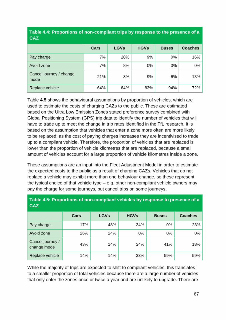
67
Table 4.4: Proportions of non-compliant trips by response to the presence of a
CAZ
Cars LGVs HGVs Buses Coaches
Pay charge 7% 20% 9% 0% 16%
Avoid zone 7% 8% 0% 0% 0%
Cancel journey / change
mode 21% 8% 9% 6% 13%
Replace vehicle 64% 64% 83% 94% 72%
Table 4.5 shows the behavioural assumptions by proportion of vehicles, which are
used to estimate the costs of charging CAZs to the public. These are estimated
based on the Ultra Low Emission Zones stated preference survey combined with
Global Positioning System (GPS) trip data to identify the number of vehicles that will
have to trade up to meet the change in trip rates identified in the TfL research. It is
based on the assumption that vehicles that enter a zone more often are more likely
to be replaced; as the cost of paying charges increases they are incentivised to trade
up to a compliant vehicle. Therefore, the proportion of vehicles that are replaced is
lower than the proportion of vehicle kilometres that are replaced, because a small
amount of vehicles account for a large proportion of vehicle kilometres inside a zone.
These assumptions are an input into the Fleet Adjustment Model in order to estimate
the expected costs to the public as a result of charging CAZs. Vehicles that do not
replace a vehicle may exhibit more than one behaviour change, so these represent
the typical choice of that vehicle type – e.g. other non-compliant vehicle owners may
pay the charge for some journeys, but cancel trips on some journeys.
Table 4.5: Proportions of non-compliant vehicles by response to presence of a
CAZ
Cars LGVs HGVs Buses Coaches
Pay charge 17% 48% 34% 0% 23%
Avoid zone 26% 24% 0% 0% 0%
Cancel journey /
change mode 43% 14% 34% 41% 18%
Replace vehicle 14% 14% 33% 59% 59%
While the majority of trips are expected to shift to compliant vehicles, this translates
to a smaller proportion of total vehicles because there are a large number of vehicles
that only enter the zones once or twice a year and are unlikely to upgrade. There are

68
a relatively small number of vehicles which make up the majority of trips and these
are expected to be the most likely to replace their vehicles in response to the CAZ
charges.
The SL-PCM model is run accounting for the reduction in non-compliant vehicle
kilometres, and resultant increases in compliant vehicle kilometres inside the zone.
From this change, the SL-PCM model is able to estimate the impact on emissions
within the zones due to the upgrade of vehicles.
Of the drivers within the zone who are upgrading, the modelling assumes they
purchase the cheapest available compliant vehicle, a second hand vehicle, and sell
their non-compliant vehicle. This means that a proportion of vehicle owners who do
not enter the zone will switch their less polluting vehicle and purchase a more
polluting one given the increased demand placed on low emission vehicles. This will
have an upward impact on total emissions outside the zone.
4.3.2 Air quality impacts
A profile of the changes in NO2 concentration associated with the implementation of
the charging CAZs is provided in Figure 4.6.

69
Figure 4.6: Reduction in average NO2 concentrations arising from the
implementation of the charging CAZ option
The light and dark shaded orange bars show the projected mean NO2 concentration with and without
the implementation of the CAZ option. The blue line shows the percentage reduction in mean NO2
concentration attributable to the implementation of CAZs (i.e. the percentage difference between the
‘with’ and ‘without’ option bars). CAZs are predicted to have their greatest impact on air quality in the
year of implementation (2020), leading to an 18% reduction in NO2 concentrations. This impact will
gradually decrease over the appraisal period, with the percentage reduction decreasing to 3% by
2029.
The absolute reduction in NO2 concentration assumes the baseline scenario is dependent on the
effectiveness of the Euro standard. If the Euro standards are less effective than predicted (as with
historical real-world operations), the impact of charging CAZs will differ from the projections presented
here.
These projections have been produced from the SL-PCM model. It is not feasible to obtain uncertainty
ranges for these estimates. Uncertainty estimates surrounding input data are also limited, but the SL-
PCM modelling incorporates the latest assumptions around emissions from each source, to reflect the
best range of evidence available. See Section 8.2 for further details.
0.03%
0.01%
0.001%
6.0%
0.02%
0.02%
0.19%
18.3%
0% 2% 4% 6% 8% 10% 12% 14% 16% 18%
Eco-driving
Vehicle Labelling
Government Vehicles
Speed Limits
Ultra Low Emission Vehicles
Scrappage
Retrofit
Clean Air Zones
Percentage reduction in average NO2 concentration arising from each option when compared to baseline in the first year where air quality impacts are expected
Option under consideration in this section Other options
0%
5%
10%
15%
20%
25%
0
10
20
30
40
50
2020 2021 2022 2023 2024 2025 2026 2027 2028 2029
Perc
enta
ge r
edu
ction in a
vera
ge N
O2
concen
tratio
n (
µg/m
3)
arisin
g fro
m C
AZ
op
tion w
hen
com
pare
d t
o t
he b
aselin
e
Ave
rag
e N
O2
co
ncentr
atio
n (
µg/m
3)
with a
nd
witho
ut
the C
AZ
option
Year
Without option (µg/m³) With option (µg/m³) Percentage reduction (%)

70
There is a large percentage reduction in NO2 in the early phase of implementation,
followed by a lower reduction over time (Fig. 4.6). This is because over time in the
absence of CAZs, the older non-compliant vehicles come to the end of their lifetimes
and are naturally replaced meaning that the fleet eventually becomes cleaner over
time (assuming that the Euro standards deliver the expected emission reductions).
CAZs are therefore bringing forward this behaviour to improve air quality more
quickly.
4.3.3 Timing
Delivery of the full programme of CAZs is anticipated to take 2 to 3 years. Where
local authorities have already done some preparatory work and are able to move
more swiftly, Government will support earlier implementation.
There are a number of stages involved in the implementation of CAZs and these can
broadly be categorised into the following:
Feasibility studies – covering data collection, transport and air quality
modelling of the local situation, options assessment, local consultation and
production and approval by the Secretary of State of a final business case (for
a scheme). Timings will vary but may take up to 18 months.
Local scheme legislation – local legislation will be required to establish the
scheme following Secretary of State approval. This may take up to six
months.
Procurement and installation of infrastructure – this primarily relates to signs
and cameras and management systems e.g. for charging. This is expected to
take up to a further six months.
Lead-in time – a period before the scheme takes effect to allow for testing of
systems and local engagement and communications to raise awareness of
the scheme and enable businesses and individuals to adjust. This is likely to
take a further six months.
Figure 4.7 provides an indicative timeline and sets out where the various
elements involved with the implementation of a charging CAZ could be
progressed in parallel.

71
Figure 4.7: Indicative timeline of CAZ measure implementation
2017 2018 2019 2020
Q3 Q4 Q1 Q2 Q3 Q4 Q1 Q2 Q3 Q4 Q1 Q2 Q3
Data collation
Local transport & air
quality modelling
Option assessment
Local consultation
Business case
development
SoS approval
Local legislation
Installation of
infrastructure
Engagement and
lead-in time
Testing
4.3.4 Government cost
These costs cover the setup and running costs of the assumed 27 charging zones. It
is expected that costs are independent of class of CAZ implemented. The costs
presented in Table 4.8 have the following attributed:
Costs are discounted values. The undiscounted setup costs are assumed to
be £270m. In the modelling, setup costs are assumed to be spent in the
earliest year all of the zones are expected to be operational (2020) and
discounted to 2017 prices, leading to a present value of £244m. In reality
much of the capital expenditure will happen prior to zones being operational;
however this simplification has been made for modelling the ten-year
appraisal period of 2020-2029.
Costs do not account for the revenues local authorities are expected to
receive from charges (these are a transfer from the public to government and
therefore are not counted in this assessment). These represent a proportion
of the running costs. Further research is underway to improve the evidence on
what this proportion is.

72
Table 4.8: Costs to government of implementing the CAZs (£m, discounted)
2020 2021 2022 2023 2024 2025 2026 2027 2028 2029 Total
Capital 244 - - - - - - - - - 244
Running 41 39 38 37 36 34 33 32 31 30 351
Total 284 39 38 37 36 34 33 32 31 30 595
4.3.5 Public cost
The costs to the public were calculated using the Fleet Adjustment Model. For more
details on the model and methodology employed, see Section 3.3.3 and Annex B.
This cost is separated into two parts:
Welfare cost – reflecting the cost to the public of meeting CAZ requirements
Loss of asset value – including the disposal of the dirtiest vehicles.
In addition to these costs, there are expected to be some traffic flow benefits to the
public as a result of the reduced number of trips taken within the zones by private
vehicles. These impacts are explained in more detail below.
Welfare loss
There will be a loss of welfare for those who own a non-compliant vehicle switching
to a more costly compliant vehicle, from foregoing the trip completely or from
diverting to avoid the zone (for more details see Section 3.3.3). The impacts of
foregoing the trip completely would only apply in areas with a Class D CAZ, given
that with other vehicles it is assumed other businesses will make the foregone
journeys of those that cannot, and gain a corresponding benefit (so the impact on
business journeys is neutral).
The cost of foregone and diverted trips is valued by estimating the number of days
within the zone that are cancelled or diverted and multiplying this by half of the value
of the charge to enter the zone. This is based on the fact that the cost of changing
behaviour must be less than the charge. For some drivers the cost will be close to
zero (those where the alternative diverted route does not add a meaningful cost), for
some the cost will be just under the full value of the charge. Therefore, dividing the
charge by two is a good approximation of the likely welfare cost.

73
Table 4.9: Welfare cost to society of CAZs (£m, discounted)
2020 2021 2022 2023 2024 2025 2026 2027 2028 2029 Total
Upgrade cost 403 312 166 117 66 41 24 14 8 5 1,157
Foregone trip
cost 61 49 38 29 22 16 10 7 4 3 238
Diverted trip
cost 237 188 146 111 82 59 39 26 16 10 914
Total welfare
cost 700 549 349 257 170 115 74 47 29 18 2,309
Loss of asset value
Encouraging the shift towards cleaner vehicles will reduce the value of the older,
more polluting vehicles, incurring a loss of asset value for the owners of such
vehicles. This impact is assumed to be a one-off cost in the first year of
implementation, as this is when a proportion of vehicles are upgraded. The lost value
of the vehicles that will be scrapped will total an estimated £341m in present values.
Traffic flow improvement benefits
As a result of the behavioural changes brought about by the CAZs, there is expected
to be a reduction in the total number of vehicle kilometres driven due to some
journeys being cancelled or individuals switching to public transport. This will lead to
less congestion, which will bring benefits to those who are still using the roads. The
total value of these benefits is estimated to be £718m in present values. It is possible
that the improvements in traffic flow will create a rebound effect by making travelling
on these roads more appealing and thus encouraging more vehicles to use these
roads. However, this effect is assumed to be negligible compared to the effects of
the CAZ charges. As a result, it has not been monetised.
4.3.6 Health benefit
Air quality is projected to improve over time as the vehicle fleet renews, controls on
emissions from industrial sources become tighter, and domestic combustion
becomes cleaner. Therefore, the health benefits incurred each year from CAZs will
diminish over the period because the air quality is expected to improve anyway
without this intervention. The positive impacts from reduced NO2 exposure total
£3.6bn in present value terms over the ten-year appraisal period, due to the dirtiest
vehicles being removed from the roads. This value is calculated using the damage
cost approach as outlined in Section 3.3, and covers mortality impacts only.

74
There will be a reduction of 24kt of NOx emissions across the UK over the ten-year
period assessed. This has been calculated using the SL-PCM model (see Section
2.1). Table 4.10 demonstrates the emission changes experienced in the UK as a
result of CAZs being implemented.
Table 4.10: Changes in national NOx emissions resulting from CAZs (kt/year)
2020 2021 2022 2023 2024 2025 2026 2027 2028 2029 Total
Inside zone -9.2 -7.8 -6.5 -5.2 -3.8 -2.5 -2.1 -1.7 -1.2 -0.8 -40.8
Outside zone 2.4 3.2 2.9 2.5 1.9 1.3 1.1 0.9 0.7 0.4 17.3
Total -6.7 -4.7 -3.6 -2.7 -2.0 -1.3 -1.0 -0.8 -0.6 -0.4 -23.6
There is expected to be a reduction in emissions in the area just outside the zone,
due to lower emission vehicles replacing high emission vehicles when entering the
zone. However, in the wider area outside the zone in the UK as a whole there will be
an increase in emissions from the dirty vehicles being sold to those unaffected by the
zone. The impact is a net increase of NOx emissions outside the zone of
approximately 17,300 tonnes (Table 4.10).
However, exposure to NO2 will be lower outside the zone as a result of the policy.
This is because emissions are likely to increase in areas of low population density
but fall just outside the zone where the population density is high. As a result, there
is expected to be a positive impact on health across the entire outside zone area
overall.
Table 4.11: Valuation of NOx emissions change from CAZs (£m, discounted)
2020 2021 2022 2023 2024 2025 2026 2027 2028 2029 Total
Inside zone 725 610 498 389 283 180 146 114 82 51 3,076
Outside
zone 167 110 83 61 42 26 19 14 10 5 536
Total 892 720 580 449 325 205 165 128 91 56 3,612
4.3.7 Greenhouse gas emissions
The implementation of CAZs is expected to lead to a reduction in greenhouse gas
(GHG) emissions, as the oldest, most polluting vehicles are expected to leave the
fleet and be replaced with cleaner vehicles, and some car journeys will be cancelled
and not replaced. This is because the new vehicles purchased as a result of the
CAZs will push down the prices of older cars across the national market leading to
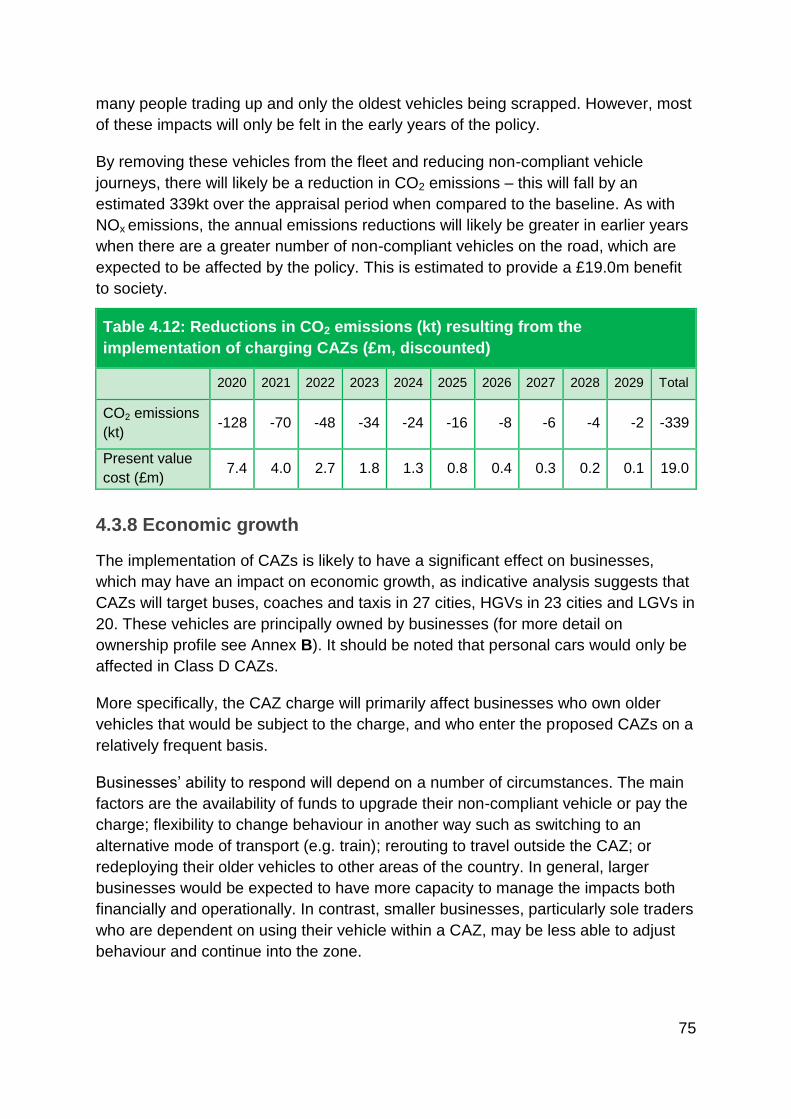
75
many people trading up and only the oldest vehicles being scrapped. However, most
of these impacts will only be felt in the early years of the policy.
By removing these vehicles from the fleet and reducing non-compliant vehicle
journeys, there will likely be a reduction in CO2 emissions – this will fall by an
estimated 339kt over the appraisal period when compared to the baseline. As with
NOx emissions, the annual emissions reductions will likely be greater in earlier years
when there are a greater number of non-compliant vehicles on the road, which are
expected to be affected by the policy. This is estimated to provide a £19.0m benefit
to society.
Table 4.12: Reductions in CO2 emissions (kt) resulting from the
implementation of charging CAZs (£m, discounted)
2020 2021 2022 2023 2024 2025 2026 2027 2028 2029 Total
CO2 emissions
(kt) -128 -70 -48 -34 -24 -16 -8 -6 -4 -2 -339
Present value
cost (£m) 7.4 4.0 2.7 1.8 1.3 0.8 0.4 0.3 0.2 0.1 19.0
4.3.8 Economic growth
The implementation of CAZs is likely to have a significant effect on businesses,
which may have an impact on economic growth, as indicative analysis suggests that
CAZs will target buses, coaches and taxis in 27 cities, HGVs in 23 cities and LGVs in
20. These vehicles are principally owned by businesses (for more detail on
ownership profile see Annex B). It should be noted that personal cars would only be
affected in Class D CAZs.
More specifically, the CAZ charge will primarily affect businesses who own older
vehicles that would be subject to the charge, and who enter the proposed CAZs on a
relatively frequent basis.
Businesses’ ability to respond will depend on a number of circumstances. The main
factors are the availability of funds to upgrade their non-compliant vehicle or pay the
charge; flexibility to change behaviour in another way such as switching to an
alternative mode of transport (e.g. train); rerouting to travel outside the CAZ; or
redeploying their older vehicles to other areas of the country. In general, larger
businesses would be expected to have more capacity to manage the impacts both
financially and operationally. In contrast, smaller businesses, particularly sole traders
who are dependent on using their vehicle within a CAZ, may be less able to adjust
behaviour and continue into the zone.

76
There is a scarcity of available evidence on the proportion and characteristics of
businesses that would absorb costs, those that would pass these on to customers,
and those that may go out of business as a result. This information will be collected
during implementation of the policy.
The TfL feasibility study for the London Low Emission Zone (2006) provided an
overview of the impacts on different sectors of the economy that are most likely to be
affected financially by the implementation of the LEZ58. Whilst much of this
information is relevant to the assessment of the zones where CAZs will be
implemented, London is unique in size, fleet composition, and business
demographics. Therefore, it is important to bear in mind that the information derived
from the TfL findings may have some limitations.
TfL found that the transport and storage, construction sectors and commuter
services were those likely to be most impacted. It was anticipated that the necessary
costs of compliance (which would vary for different operators depending on their
fleets) will be largely absorbed by vehicle owners within these sectors because of the
very competitive markets in which they operate.
CAZs should also deliver benefits to economic growth through improved air quality.
This would reduce the number of absences from work, distracted performance or
employee deaths, which all impact on business productivity (for more details see
Section 8 on sensitivities). The policy would also stimulate demand for new vehicles,
which will have a positive impact on vehicle manufacturers and therefore encourage
economic growth.
4.3.9 Conclusion
Table 4.13 summarises the results of the analysis of charging CAZs. It shows the
expected average reduction in concentrations in 2020 (which is the modelled start
year of the scheme) and the present values of impacts on Government, the public,
and the benefits to society as a result of improved air quality and reduced
greenhouse gas emissions. These impacts have been appraised over a ten-year
period.
58 Report for Transport for London, ‘Proposed London Low Emission Zone Economic And Business
Impact Assessment: Non-Technical Summary’, 2006 <http://content.tfl.gov.uk/economic-impact-
assessment-non-technical-summary.pdf>

77
Table 4.13: Summary of impacts of the charging CAZ assessmentI
Results
Confidence in
assessment Comments
First year air
quality
improvementII
8.6µg/m3 in
2020
Established
(preliminary
assumptions)
This is the average reduction in
the maximum concentration for
non-compliant areas
Total reduction in
NOx emissionIII
24kt over ten
years
Timing to impactIV
1-3 years N/A Time taken dependent on the
state of LA preparation as well
as procurement timing
Health impact
£3,600m Established
(preliminary
assumptions)
The net monetised impact of the
change in NOx emissions
resulting from this measure
Government
impact
-£600m Established
(preliminary
assumptions)
The cost to Government of
setting up and administering the
CAZs over the ten year period
Public impact
-£1,900m Established
(preliminary
assumptions)
The net of the costs of both lost
welfare and the loss of asset
value with the benefits of
improvements in traffic flows
Greenhouse gas
emissions impact
£19m Established
(preliminary
assumptions)
The net monetised impact of the
change in CO2e emissions
resulting from this measure
Economic growth
impact
Positive and
negative
impacts
N/A Positive impacts through
improved air quality and higher
new vehicle purchases.
Negative impacts through
increased costs to businesses.
I All monetised impacts are present values, discounted to 2017 prices, appraised over 2020-29.
II This is the reduction in average NO2 concentrations, in the first year where air quality impacts
are expected to arise as a result of the implementation of the option. This is relative to the
baseline projection for the option in the particular year specified.
III This is the total reduction in NOx emissions resulting from this policy option over its ten-year
appraisal period. This is in comparison to the baseline projection for the option over the same ten-
year appraisal period.
IV Indicative timings are provided for all options as either <1, 1-3 or >3 years.

78
5. Measures to support Clean Air Zones
5.1 Introduction
While local action through CAZs is one of the most effective measures to reduce
NO2 emissions, they could affect many individuals and businesses. This section
analyses measures that could be introduced to support the transition to CAZs. They
would do so by reducing the costs of compliance for individuals or businesses, or by
lowering the level of charging required, or possibly removing it entirely. These
measures are:
Retrofit
Scrappage
Support for Ultra Low Emission Vehicles (ULEVs)
Each of these has been assessed in turn, using the same criteria applied to the CAZ
assessment and as outlined in Section 3.3.
5.2 Retrofit
5.2.1 Introduction
Retrofitting vehicles can reduce the amount of NOx emitted. This policy considers
retrofit schemes for buses, HGVs, and black taxis. Retrofit installs two technologies:
selective catalytic reduction (SCR) for buses and HGVs, and liquefied petroleum gas
(LPG) retrofit for black taxis. SCR is the technology used in the latest Euro 6 buses
and HGVs to minimise NO2 emissions. LPG retrofit for black taxis has been
undertaken within the Clean Vehicle Technology Fund, and evaluation evidence
showed emissions after retrofit equivalent to a petrol engine.
The theoretical maximum potential scheme assumed that all pre-Euro 6 buses,
HGVs, and black taxis are retrofitted. The scheme considered in this section scales
the measure to what is considered a more feasible level of retrofitting. The chief
constraint on retrofit is market capacity. Policy experts have estimated that it may be
possible to retrofit up to 6,000 buses, 4,400 black taxis, and 2,000 HGVs over a
three-year period. This is based on an assessment of market capacity, based on
working with retrofit suppliers.

79
The most significant uncertainty is likely to be market capacity. Retrofit of buses is
well established. Retrofit of HGVs uses the same technology; however, there may be
design issues with installing retrofit technology within the design of existing vehicles.
Retrofit of taxis has been undertaken to date, but only at limited scale.
5.2.2 Air quality impacts
The impact of retrofitting 6,000 buses, 4,400 taxis, and 2,000 HGVs (around 12,400
vehicles in total) has been estimated. This would result nationally in 6% of taxis,
0.4% of HGVs, and 19% of buses being retrofitted. The policy is designed so that
retrofitted vehicles are targeted at those delivering highest value for money. That is
Euro 3-5 buses; Euro 5 HGVs and Euro 5 taxis. The assessment for the retrofit
option is made using the scrappage/retrofit model described in Section 3.3.3.
A profile of the changes in NO2 concentration associated with the implementation of
the retrofit option is provided in Figure 5.1.
5.2.3 Timing
A retrofit accreditation scheme is currently being developed to test, validate, and
certify retrofitted vehicles to ensure that when retrofit solutions are rolled out all
suppliers are in a position to deliver solutions that reach the required standard. The
scheme is expected to be in place by the end of 2017 to early 2018.
A retrofit grant scheme would need to be established where organisations could bid
in for funding to retrofit vehicles with accredited technology – it is estimated to take
between one and three years to deliver retrofitted vehicles.
Previous retrofit grant schemes, such as the Clean Bus Technology Fund (CBTF)
and Clean Vehicle Technology Fund (CVTF), have successfully implemented some
technologies and in particular have focused on buses. There may be challenges to
extending retrofitting to other types of vehicle successfully. In addition, retrofitting
companies will need to have the capacity to meet the demand. Any grant funding
could be staggered across the funding period.
5.2.4 Government cost
The costs to administer the proposed options have not been estimated at this stage.
These costs are unlikely to be significant in comparison to the costs of retrofitting
vehicles, and therefore excluding these is unlikely to materially affect the
conclusions.

80
Government is assumed to incur the full cost of retrofit, estimated at £170m. The
assumed costs of retrofit are as follows:
Cost of SCR: £17,000
Cost of LPG: £8,000
These have been estimated based on existing retrofit schemes undertaken by
Government. The cost of retrofitting HGVs is assumed to be the same as the cost for
retrofitting buses. Total costs were estimated by multiplying the retrofit cost by the
number of vehicles retrofitted. In the modelled option, retrofit is assumed to take
place in 2018.
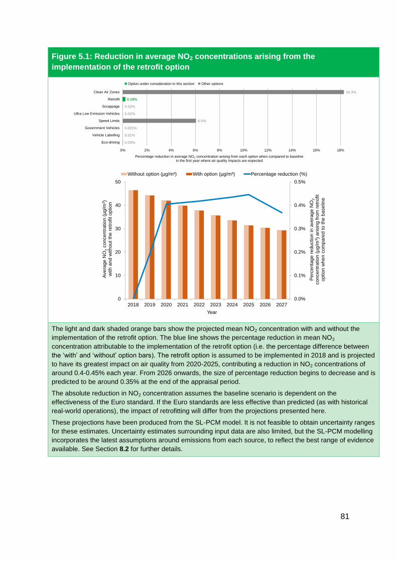
81
Figure 5.1: Reduction in average NO2 concentrations arising from the
implementation of the retrofit option
The light and dark shaded orange bars show the projected mean NO2 concentration with and without the
implementation of the retrofit option. The blue line shows the percentage reduction in mean NO2
concentration attributable to the implementation of the retrofit option (i.e. the percentage difference between
the ‘with’ and ‘without’ option bars). The retrofit option is assumed to be implemented in 2018 and is projected
to have its greatest impact on air quality from 2020-2025, contributing a reduction in NO2 concentrations of
around 0.4-0.45% each year. From 2026 onwards, the size of percentage reduction begins to decrease and is
predicted to be around 0.35% at the end of the appraisal period.
The absolute reduction in NO2 concentration assumes the baseline scenario is dependent on the
effectiveness of the Euro standard. If the Euro standards are less effective than predicted (as with historical
real-world operations), the impact of retrofitting will differ from the projections presented here.
These projections have been produced from the SL-PCM model. It is not feasible to obtain uncertainty ranges
for these estimates. Uncertainty estimates surrounding input data are also limited, but the SL-PCM modelling
incorporates the latest assumptions around emissions from each source, to reflect the best range of evidence
available. See Section 8.2 for further details.
0.03%
0.01%
0.001%
6.0%
0.02%
0.02%
0.19%
18.3%
0% 2% 4% 6% 8% 10% 12% 14% 16% 18%
Eco-driving
Vehicle Labelling
Government Vehicles
Speed Limits
Ultra Low Emission Vehicles
Scrappage
Retrofit
Clean Air Zones
Percentage reduction in average NO2 concentration arising from each option when compared to baseline in the first year where air quality impacts are expected
Option under consideration in this section Other options
0.0%
0.1%
0.2%
0.3%
0.4%
0.5%
0
10
20
30
40
50
2018 2019 2020 2021 2022 2023 2024 2025 2026 2027
Perc
enta
ge r
edu
ctio
n in
avera
ge N
O2
co
nce
ntr
atio
n (
µg/m
3)
arisin
g f
rom
re
trofit
op
tio
n w
he
n c
om
pa
red t
o t
he
ba
se
line
Ave
rage
NO
2con
cen
tra
tio
n (
µg
/m3)
with a
nd
with
out
the
re
trofit
optio
n
Year
Without option (µg/m³) With option (µg/m³) Percentage reduction (%)

82
5.2.5 Public cost
As the full cost of retrofit is paid for by Government, there are no direct costs to
society. It is assumed that the costs to companies of taking vehicles out of service
are mitigated by getting vehicles retrofitted when they are out of circulation or in the
case of taxis on days when the vehicle is not being used. It has been assumed that
vehicle owners do not face a cost when retrofitting vehicles as they can manage
fleets and use vehicles not in service.
5.2.6 Health benefit
NOx emissions are expected to fall as a result of retrofit. The difference in NOx
before and after retrofit is estimated over the lifetime of the vehicle over the period to
2027. The estimated reduction in NOx over the appraisal period is estimated to be
around 10kt.
As noted, for buses and taxis the damage cost for large urban areas was applied to
total emission savings, and for HGVs the transport average damage cost was
applied, and discounted to provide an estimate of the health impacts of the options.
It is estimated that the retrofit option could result in a present value health benefit of
around £440m.
5.2.7 Greenhouse gas emissions
Evidence from bus retrofit schemes has shown they have had no impact on CO2
emissions. Evidence from LPG suggests that it has a similar CO2 content to diesel
on a per kilometre basis. Therefore, it is assumed there would be no CO2 impacts as
a result of implementing this option.
5.2.9 Economic growth
There are likely to be some benefits from an expansion of retrofit. The retrofitting
procedure has to be undertaken in the UK and is relatively labour intensive, thus this
option is likely to lead to increased demand for the skills and services to perform
retrofitting. Therefore, it is likely to contribution to UK jobs and employment in the
short term, as well as promoting overall growth in the retrofit market.
5.2.10 Conclusion
Table 5.2 summarises the results for this option.

83
Table 5.2: Summary of impacts of the retrofit assessmentI
Results
Confidence in
assessment Comments
First year air quality
improvementII 0.09µg/m3 in
2019
Established
(preliminary
assumptions)
This is the average reduction in
the maximum concentration for
all UK reporting zones
Total reduction in
NOx emissionsIII
10kt over ten
years
Timing to impactIV
1-3 years N/A Time taken dependent on ability
of market to deliver mass retrofit
and desire from vehicle owners
Health impact
£440m Established
(preliminary
assumptions)
The net monetised impact of the
change in NOx emissions
resulting from this measure
Government impact
-£170m Established
(preliminary
assumptions)
The cost to Government of this
measure assuming it covers full
cost of retrofit
Public impact
Negligible Established
(preliminary
assumptions)
Government covers cost of
retrofit, so no cost accrued
Greenhouse gas
emissions impact
Negligible Established
(preliminary
assumptions)
Impact assumed to be zero as
LPG and diesel have similar
CO2e emissions
Economic growth
impact
Benefits
through
expansion of
retrofit industry
N/A Retrofitting vehicles is a labour
intensive process. Thus
increases in demand for these
transformations will increase
employment and so growth
I All monetised values are present values, discounted to 2017 prices, appraised over 2018-27.
II This is the reduction in average NO2 concentrations, in the first year where air quality impacts are
expected to arise as a result of the implementation of the option. This is relative to the baseline
projection for the option in the particular year specified.
III This is the total reduction in NOx emissions resulting from this policy option over its ten-year
appraisal period. This is in comparison to the baseline projection for the option over the same ten-
year appraisal period.
IV Indicative timings are provided for all options as either <1, 1-3 or >3 years.

84
5.3 Scrappage
5.3.1 Introduction
Older vehicles associated with previous Euro standards emit substantially more pollution per kilometre than newer vehicles. Consequently, Government intervention in the form of a vehicle scrappage scheme could reduce emissions by increasing the turnover in the fleet.
The maximum potential of this measure explored in Section 3.4 illustrated that the
cost associated with scrapping all pre-Euro 6 diesel cars and vans (around 10 million
vehicles) could be around £60 billion. However, this cost is likely to be an
underestimate as consumers would likely need to be offered even higher grant levels
to incentivise 100% take-up of the scheme.
This section considers a smaller scale option, assumed for the analysis to be a
national scrappage scheme open to drivers of diesel Euro 1-5 cars and drivers of
petrol Euro 1-3 cars. It is assumed to be open to all drivers of such vehicles, so is not
targeted at particular geographic areas or characteristics of the drivers. It is also
assumed that vehicles would have to be replaced with a new Battery Electric Vehicle
(BEV), which would enable greater emissions savings per vehicle than if plug-in car
hybrid vehicles (PHEVs) or Euro 6 conventional vehicles were offered as
replacements. This option was selected as it aligns with wider Government ambition
to support Ultra Low Emission Vehicles (ULEVs), can be tied in with the existing
Plug-In Car Grant scheme, and does not involve replacing diesel with petrol, which
could have an impact on greenhouse gas emissions. The modelling assumes that
15,000 vehicles (9,000 diesel vehicles and 6,000 petrol vehicles) are scrapped and
replaced with BEVs.
This is just one way in which a scrappage scheme could be designed, and is for
illustrative purposes only. Other approaches include targeting vehicles from a
specific sector, targeting by geography, or narrowing the individuals eligible to apply
for a scrappage scheme.
The market for vans is currently dominated by conventional internal combustion
engines (ICEs). Although it is expected that the market share of low emission vans
(both battery electric and plug-in hybrids) will increase in the future, vans have been
excluded from this analysis because the expected take up of BEVs, especially
amongst owners of pre-Euro 6 vans, is expected to be low.
The way the scrappage proposal outlined might be expected to improve air quality is
by increasing fleet turnover and therefore reducing the average age of the vehicle
fleet. Assuming other factors that influence emissions remain unchanged (e.g.
distance travelled) this will result in reduced emissions.

85
The NPV for this option is estimated to be -£20 million. It is negative because the
estimated costs of offering grants to the participants of the scheme significantly
outweigh the benefits that it has been possible to quantify.
It should be noted that there are a range of non-monetised benefits associated with
the promotion and early uptake of ULEVs to ensure that Government can stay on a
path consistent with its targets. These benefits are likely to be significant – indeed
cost-benefit analysis over a period to 2050 shows electric vehicle support to be cost
effective. However, it has not been possible to monetise this as part of the analysis
presented in this report due to the relatively short appraisal period.
The key assumptions underpinning the modelling are as follows:
The start year of the scheme is assumed to be 2019;
The impacts of the scheme start to feed through in 2020;
The scheme duration is for one year only; and
Impacts are appraised over ten years from the start of the scheme (2019-
2028).
The most significant uncertainty relating to this option is the likely take up of the
scheme presented. A key assumption underpinning the analysis is that the assumed
grant levels are sufficiently high to:
Incentivise vehicle owners to scrap their vehicles earlier than they otherwise
would have done; and
Incentivise these vehicle owners to participate in the scheme and buy new
vehicles with the scrappage payment instead of used vehicles; and/or
Incentivise around 15,000 Euro 1-5 diesel/Euro 1-3 petrol car owners to buy a
BEV if they are also offered an additional grant incentive from this scheme of
£6,000 alongside £2,000 to cover the residual value of their vehicle. These
estimates (on take-up and grant levels) have been benchmarked using similar
schemes/existing evidence.
However, these assumptions may not be reasonable. It has not been possible to
quantify the premium that vehicle owners are likely to need (over and above the
residual asset value of their vehicle) to incentivise them to change behaviour (scrap
their car, buy a new car and/or buy a BEV). This means the uptake of the scheme
could be higher or lower than assumed.

86
5.3.2 Air quality impacts
The impact of scrapping 15,000 older petrol and diesel vehicles and replacing them
with BEVs was estimated to deliver a 0.008μg/m3 reduction in average NO2
concentrations in 2020 (the first year in which air quality impacts from the scheme
have been assumed). This would result in around 0.05% of the total stock of
conventionally fuelled vehicles (ICEs) in 2019 being scrapped. A profile of the
changes in NO2 concentration associated with the implementation of the scrappage
option is provided in Figure 5.4.

87
Figure 5.4: Reduction in average NO2 concentrations following the implementation
of the scrappage option
The light and dark shaded orange bars show the projected mean NO2 concentration with and without the
implementation of the scrappage option. The blue line shows the percentage reduction in mean NO2
concentration attributable to the implementation of the scrappage option (i.e. the percentage difference
between the ‘with’ and ‘without’ option bars). This option is assumed to be implemented in 2019 and is
predicted to have a low but stable impact on air quality throughout the appraisal period, contributing a
reduction in NO2 concentrations of around 0.02% each year from 2020 to 2028.
The absolute reduction in NO2 concentration assumes the baseline scenario is dependent on the
effectiveness of the Euro standard. If the Euro standards are less effective than predicted (as with
historical real-world operations), the impact of scrappage will differ from the projections presented here.
These projections have been produced from the SL-PCM model. It is not feasible to obtain uncertainty
ranges for these estimates. Uncertainty estimates surrounding input data are also limited, but the SL-PCM
modelling incorporates the latest assumptions around emissions from each source, to reflect the best
range of evidence available. See Section 8.2 for further details.
0.03%
0.01%
0.001%
6.0%
0.02%
0.02%
0.19%
18.3%
0% 2% 4% 6% 8% 10% 12% 14% 16% 18%
Eco-driving
Vehicle Labelling
Government Vehicles
Speed Limits
Ultra Low Emission Vehicles
Scrappage
Retrofit
Clean Air Zones
Percentage reduction in average NO2 concentration arising from each option when compared to baseline in the first year where air quality impacts are expected
Option under consideration in this section Other options
0.000%
0.005%
0.010%
0.015%
0.020%
0.025%
0.030%
0
10
20
30
40
50
2019 2020 2021 2022 2023 2024 2025 2026 2027 2028P
erc
enta
ge r
eduction in a
vera
ge N
O2
concentr
atio
n (
µg/m
3)
arisin
g fro
m s
cra
ppage
option w
hen c
om
pare
d t
o t
he b
aselin
e
Avera
ge N
O2
concentr
atio
n (
µg/m
3)
with a
nd w
ithout
the s
cra
ppage o
ption
Year
Without option (µg/m³) With option (µg/m³) Percentage reduction (%)

88
5.3.3 Timing
The design of any scrappage scheme will determine the exact processes required to
implement it. There are a number of factors that would drive the timescale including
potential need for new legislation, getting major project assurances in place,
addressing any state aid challenges, developing contracts and agreements with
industry and identifying organisations to set up and administer the scheme.
It is anticipated that it would take at a minimum 18 to 24 months before any
scrappage scheme could be launched.
5.3.4 Government cost
The main cost to Government that has been quantified is the cost of the grants paid
to participants of the scheme. The discounted cost to Government is estimated to be
around £110m (2017 prices and base year).
Under this scheme, 15,000 Euro 1-5 diesel cars/Euro 1-3 petrol cars are replaced
with electric cars. The grant level that has been assumed for this option is £8,000.
This is based on the size of the grant awarded in a similar scrappage scheme in
France, which achieved a similar level of take-up. £8,000 is significantly higher than
the £2,000 residual value of the vehicle that would be scrapped, which reflects the
fact that additional incentives are likely to be needed to incentivise people to change
their cars earlier and move to a BEV.
The costs to administer any scrappage scheme have not been estimated at this
stage. The costs will be dependent on how any scheme is delivered. If industry were
to participate (in line with the previous UK scrappage scheme in 2009), this could
lower the costs of operating a scheme for central government as the costs could be
shared with industry. To illustrate the magnitude of these costs, the annual
administrative costs associated with the previous scheme were estimated to be
around £450,00059 (2009 prices); this estimate includes staff and consulting costs
plus other fees. The impact on taxes has not been assessed at this stage.
5.3.5 Public cost
The key assumption underpinning the scrappage analysis is that vehicles are
scrapped sooner than they would have been had there been no scrappage scheme.
Consequently, society loses the residual value of vehicles that are scrapped sooner.
This welfare cost has been valued by quantifying the residual value of the vehicles
59 The estimate above has been scaled up to cover one whole year. Actual estimate was £331,000 (2009 prices
over 9 months).

89
by Euro standard and multiplying these by the expected number of vehicles that will
be scrapped. The discounted costs to society associated with the lost residual value
of the vehicles scrapped are estimated to be around £10m over the appraisal period.
In general economic terms, any form of subsidy offered results in a deadweight loss
(reduction in net economic benefits) to society. Economic inefficiency (loss to
society) could arise as a result of some consumers taking up the scheme even
though the benefit to them of the BEV is less than the real cost of the BEV. The
discounted costs to society associated with the deadweight loss are estimated to be
around £40m over the appraisal period.
Given rational consumer choice, it has been assumed that the additional cost to
consumers of purchasing a BEV is offset by the operating cost savings and the
additional utility gained by the consumer. This means that the first three years
(based on the assumed average length of ownership) of operating costs are
assumed to be accounted for in the original decision to purchase. The operating cost
savings to society (after the assumed three year ownership period) have been
quantified and are estimated to be around £10m (2017 price and base year) over
the appraisal period. The measure will also result in a transfer to consumers (the
grant that the government pays out to those that take up the scheme). The
discounted benefits to society associated with the transfer are estimated to be
around £110m over the appraisal period.
The total discounted net benefit (costs of lost residual value and deadweight and
benefits of the transfer to consumers and benefits of operating cost savings) to
society associated with this measure are estimated to be around £70m over the
appraisal period.
5.3.6 Health benefit
NOx emissions would be expected to fall as a result of the change in the fleet
composition. NOx emission factors by Euro standard from the NAEI were used for the
different vehicle types to assess the impact. The estimated reduction in NOx over the
appraisal period is estimated to be around 0.4kt for this option.
The transport average damage costs were then applied to the total emissions
savings and discounted to provide an estimate of the health impacts. It is estimated
that the measure could result in a health benefit of around £10m.
5.3.7 Greenhouse gas emissions
Greenhouse gas (GHG) emissions would be expected to fall as a result of the
change in the fleet composition. CO2 emission factors from the NAEI split by Euro

90
standard and vehicle type were used to assess the impact of the measure. The
estimated reduction in CO2 is estimated to be around 0.2MtCO2.
The social costs of carbon were then applied to the total emissions saving and
discounted to provide an estimate of the GHG impacts of the options. It is estimated
that the measure could result in around £10m in benefits from GHG emission
savings over the ten-year appraisal period.
The current assessment does not consider the impact of GHG emissions from the
additional electricity consumed by the BEVs, as these are included in the cost of
electricity through its inclusion in the EU emissions trading scheme.
5.3.8 Economic growth
In the short term, scrappage schemes could have a small positive impact on
economic growth, although this will depend on the size of any scheme and rates of
uptake. This is because they may lead to an increase in demand for new cars. The
primary objective of the previous national scrappage scheme was to provide a boost
to the UK car industry by attempting to offset the dramatic decline in car sales at the
time (as a result of the recession). The longer-term impacts of scrappage schemes
on economic growth are more uncertain.
5.3.9 Conclusion
Table 5.6 summarises the results for this option.
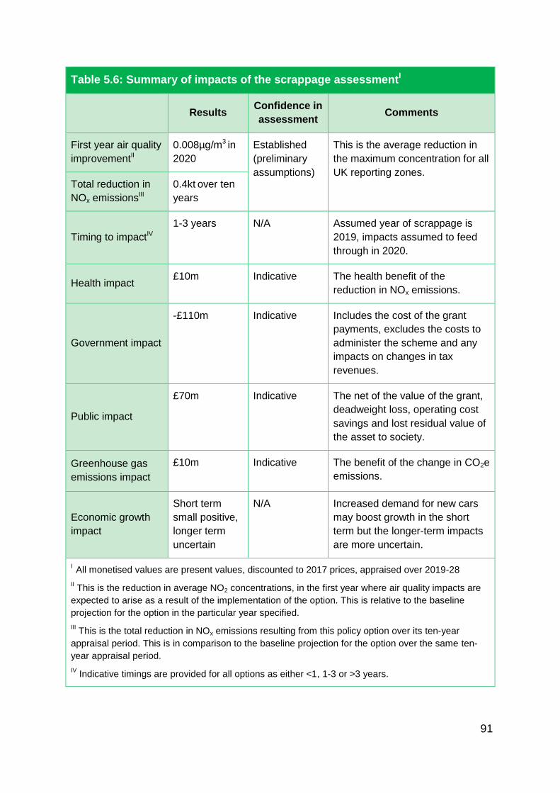
91
Table 5.6: Summary of impacts of the scrappage assessmentI
Results
Confidence in
assessment Comments
First year air quality
improvementII 0.008µg/m3 in
2020
Established
(preliminary
assumptions)
This is the average reduction in
the maximum concentration for all
UK reporting zones. Total reduction in
NOx emissionsIII
0.4kt over ten
years
Timing to impactIV
1-3 years N/A Assumed year of scrappage is
2019, impacts assumed to feed
through in 2020.
Health impact £10m Indicative The health benefit of the
reduction in NOx emissions.
Government impact
-£110m Indicative Includes the cost of the grant
payments, excludes the costs to
administer the scheme and any
impacts on changes in tax
revenues.
Public impact
£70m Indicative The net of the value of the grant,
deadweight loss, operating cost
savings and lost residual value of
the asset to society.
Greenhouse gas
emissions impact
£10m Indicative The benefit of the change in CO2e
emissions.
Economic growth
impact
Short term
small positive,
longer term
uncertain
N/A Increased demand for new cars
may boost growth in the short
term but the longer-term impacts
are more uncertain.
I All monetised values are present values, discounted to 2017 prices, appraised over 2019-28
II This is the reduction in average NO2 concentrations, in the first year where air quality impacts are
expected to arise as a result of the implementation of the option. This is relative to the baseline
projection for the option in the particular year specified.
III This is the total reduction in NOx emissions resulting from this policy option over its ten-year
appraisal period. This is in comparison to the baseline projection for the option over the same ten-
year appraisal period.
IV Indicative timings are provided for all options as either <1, 1-3 or >3 years.

92
5.4 Ultra Low Emission Vehicles
5.4.1 Introduction
The plug-in car grant is an existing scheme set up by Government to incentivise the
take-up of both battery operated electric vehicles and plug-in hybrid electric vehicles
(collectively referred to as Ultra Low Emission Vehicles (ULEVs) from this point
forward) through a subsidy on the purchase price of new ULEVs. Section 3.4
explores the theoretical maximum potential of motorists switching to battery electric
vehicles. This section considers the impact of a more feasible proposal of extending
the length of the existing scheme at current grant levels. For the purposes of the
modelling scenario, it is assumed the criteria of the current scheme will continue to
apply only to cars. Thus, the impact of this measure on both vans and motorcycles
has not been measured.
For illustrative purposes, this option assumes an additional funding pot of £300m
over the next three years, to the end of this parliament. The costs to administer this
proposed option have been assumed as marginal as this builds on an existing
scheme, therefore the modelling assumes that the full funding pot will be utilised
through the scheme and that demand perfectly fits annual budgets. This would mean
a total of around 160,000 ULEVs being purchased over the next three years. Of
these, the funding is assessed to provide an additional 60,000 ULEVs being
purchased as a result of this measure (the other 100,000 ULEVs would have been
purchased anyway).
The grant will be lower, on average, than the additional cost to the consumer of
purchasing an ULEV over a convention vehicle. However, consumers continue to
buy new ULEVs, in part due to the cost savings that occur in tax and operating costs.
The modelling therefore looks at both the cost to Government of the scheme, but
also the wider consumer benefits, operating costs and the deadweight loss
associated with a subsidy type scheme.
The emission reductions and health impacts from these additional ULEVs have been
modelled against a baseline scenario that they would otherwise have been newly
purchased conventional cars (Euro 6 standard), split equally between petrol and
diesel variants (based on existing evidence of purchasing decisions). Consequently,
the reduction in NO2 concentrations results from this switch from conventional cars
to ULEVs. There is not a complete reduction in NOx emissions, as some will continue
to be released from the plug-in hybrid vehicles when they are running on their
conventional engines. In addition, the impact on emissions is reduced, as newer
conventional cars tend to emit relatively lower levels of NOx than their older
counterparts do.

93
Initial modelling of these proposals shows that the net present value of this measure
is negative. This is mainly because the additional cost of the grants to Government
outweighs the estimated benefits to society over the course of the ten-year appraisal.
However, the modelling considers the impact of additional funding for the plug-in car
grant in isolation, without the other parts of the Government’s wider programme of
support for ULEVs and associated benefits.
As with other policies outlined in this report, it should be noted that there are a range
of non-monetised benefits associated with promoting early uptake of ULEVs, which it
has not been possible to quantify in this modelling. The short appraisal period used
fails to capture the full lifespan of the cars bought using the grant. Thus the potential
associated long-term benefits of increased ULEV adoption, such as greater public
understanding, acceptance, and uptake of ULEVs, are not accounted for at this early
stage. Increased acceptance and uptake of ULEVs should ensure that we stay on a
path consistent with our carbon budgets. These benefits are likely to be significant;
cost-benefit analysis over a period to 2050 shows ULEV support to be cost effective.
5.4.2 Air quality impacts
As ULEVs have low NOx emissions (and Battery Electric Vehicles have none), the air
quality improvements stem from the assumption that each additional ULEV is
replacing a conventional car. The vehicles being replaced are assumed to be new
Euro 6 cars (i.e. that consumers would have bought a new car without the policy),
split equally between petrol and diesel. As Euro 6 standard vehicles emit significantly
less NOx compared to older variants, replacing these newer vehicles with ULEVs has
a correspondingly lower air quality impact than replacing older conventional vehicles.
A profile of the changes in NO2 concentration associated with the support for ULEVs
option is provided in Figure 5.7.
5.4.3 Timings
The plug-in car grant is already established and it is envisaged that this proposal
would supplement existing funding, allowing the current grant rates to be maintained
for a longer period. This is expected to lead to increased ULEV uptake. Any
extension of the PICG could be implemented with minimal delay.
The key assumption on timing is that the integration of the additional ULEVs into the
general fleet of cars will be complete by the end of 2019. If the measure is
implemented in 2017, the air quality benefits of this proposal would begin as soon as
additional ULEVs are introduced into the fleet. However, the full effects of the policy
only become evident once the full integration of the new vehicles into the fleet is
complete.

94
Figure 5.7: Reduction in average NO2 concentrations following the implementation
of the support for Ultra Low Emission Vehicles (ULEVs) option
The light and dark shaded orange bars show the projected mean NO2 concentration with and without the
implementation of the promotion of Ultra Low Emission Vehicles (ULEV) option. The blue line shows the
percentage reduction in mean NO2 concentration attributable to the implementation of the ULEV option (i.e.
the percentage difference between the ‘with’ and ‘without’ option bars). The promotion of ULEVs option is
assumed to be implemented in 2017. Its impact on NO2 concentrations over the appraisal period is
estimated to be relatively low in magnitude overall, increasing in the first few years from a reduction of 0.02%
in the implementation year to around 0.08% in 2020. From then onwards, the increase in impact is more
gradual, starting to level off at around 0.09% by the end of the appraisal period.
The absolute reduction in NO2 concentration assumes the baseline scenario is dependent on the
effectiveness of the Euro standard. If the Euro standards are less effective than predicted (as with historical
real-world operations), the impact of ULEVs will differ from the projections presented here.
These projections have been produced from the SL-PCM model. It is not feasible to obtain uncertainty
ranges for these estimates. Uncertainty estimates surrounding input data are also limited, but the SL-PCM
modelling incorporates the latest assumptions around emissions from each source, to reflect the best range
of evidence available. See Section 8.2 for further details.
0.03%
0.01%
0.001%
6.0%
0.02%
0.02%
0.19%
18.3%
0% 2% 4% 6% 8% 10% 12% 14% 16% 18%
Eco-driving
Vehicle Labelling
Government Vehicles
Speed Limits
Ultra Low Emission Vehicles
Scrappage
Retrofit
Clean Air Zones
Percentage reduction in average NO2 concentration arising from each option when compared to baseline in the first year where air quality impacts are expected
Option under consideration in this section Other options
0.00%
0.02%
0.04%
0.06%
0.08%
0.10%
0
10
20
30
40
50
2017 2018 2019 2020 2021 2022 2023 2024 2025 2026P
erc
en
tag
e r
ed
uctio
n in
ave
rag
e N
O2
co
nce
ntr
atio
n (
µg
/m3)
arisin
g f
rom
UL
EV
o
ptio
n w
he
n c
om
pa
red
to
th
e b
ase
line
Ave
rag
e N
O2
co
nce
ntr
atio
n (
µg
/m3)
with
an
d w
ith
ou
t th
e U
LE
V o
ptio
n
Year
Without option (µg/m³) With option (µg/m³) Percentage reduction (%)

95
5.4.4 Government cost
The assumed cost to Government of this option is the funding pot of £300m to fund
the expansion and extension of the plug-in car grant. This would fund the purchase
of around 60,000 additional ULEVs, above the baseline, over the next three years.
As the cost will occur over a number of years, the discounted impact to Government
is a cost of around £290m.
It should also be noted that at this stage project running costs and complementary
infrastructure costs, such as additional charging stations if needed, have not been
quantified or accounted for.
5.4.5 Public cost
The measure will result in a transfer to consumers in the form of the grant that the
Government pays out to those that take up the scheme. The discounted impact to
society associated with the transfer is estimated to be around £140m over the
appraisal period.
Given rational consumer choice, it has been assumed that the additional cost to
consumers of purchasing a ULEV (above the grant level) is offset by the operating
cost savings and the additional personal satisfaction gained by the consumer from
owning a ULEV. There are further benefits, from reductions in operating cost
calculated as a result of moving to a ULEV, which have been calculated from year
four onwards. This means that the first three years (based on assumed average
length of ownership) operating costs are assumed to be accounted for in the original
decision to purchase. The operating cost savings to society (after the assumed
three-year ownership period) have been quantified and are estimated to be around
£30m over the appraisal period.
Other factors such as requiring a longer charging time on long distance journeys and
less noise pollution compared to conventional cars have not been quantified in this
assessment.
Therefore, the total discounted impact on society associated with this option is
estimated to be around £170m over the appraisal period.
5.4.6 Health benefit
NOx emissions are expected to reduce as a result of this measure due to additional
ULEVs entering the fleet and replacing conventional cars. Over the ten-year
appraisal period, this results in around 2kt of reduced NOx emissions.

96
The average transport damage costs are then applied in order to quantify the health
impacts of this reduction in emissions. Over this period the discounted health
benefits from this measure is estimated to be around £50m.
5.4.7 Greenhouse gas emissions
In addition to reducing emissions of NOx and other particulate matter, this measure is
also likely to impact upon the level of CO2 and greenhouse gas (GHG) emissions. As
ULEVs replace conventional cars, which emit more CO2 on average, the option will
reduce emissions overall. The total amount of CO2 reduction was estimated using
the average emission levels of the replaced vehicles, per km, and the average
vehicle kilometres travelled. This was then offset by the CO2 generated by the
additional plug-in hybrid cars.
The social cost of carbon was then applied to the net emission reductions and
discounted to provide an estimate of the GHG impacts of this option. The discounted
benefits from this reduction in GHG emissions are estimated be around £50m.
The current assessment does not consider the impact of GHG emissions from the
additional electricity consumed by the ULEVs, as these are included in the cost of
electricity through its inclusion in the EU emissions trading scheme.
5.4.8 Economic growth
In the short term, this support for increased take up of ULEVs should have a positive
impact on economic growth, especially in terms of growth in the ULEV market. There
is also the potential for increased jobs and growth linked to the design, development,
and manufacture of ULEVs in the UK as a result of increased ULEV uptake.
The ULEV market is still relatively small compared to the more established
conventional car industry and the relatively high marginal costs mean this grant
scheme should have a positive impact in helping to establish the consumer market
for ULEVs. The increased demand for ULEVs generated by this scheme should have
a positive short term impact and could lead to increased economic activity than
otherwise would have been the case.
5.4.9 Conclusion
Table 5.8 summarises the results for this option. Under the current modelling
assumptions, this policy is estimated to lead to a reduction in NOx emissions and
have positive health impacts. However, the current level of technology and
production means the initial cost of purchasing an ULEV is, on average, greater than
that of a conventional vehicle. Over the course of the appraisal period used this
higher initial cost and the government grant used to reduce this cost outweighs the
benefits discounted over time. However, these benefits will extend beyond the

97
lifetime of the appraisal conducted here as the average life of a car in the fleet is
nearer 12 years.
Overall, this policy is estimated to have a net present value of around -£20m. It is
important to note that the above assessment does not take into account the
significant signalling impact of increased ULEV uptake. It is possible that increased
adoption at this early stage could lead to associated long-term benefits of increased
public understanding, acceptance, and uptake of ULEVs and associated growth of
supporting infrastructure all of which would provide longer-term benefits that have
not been quantified.

98
Table 5.8: Summary of impacts of the ULEV assessmentI
Results
Confidence in
assessment Comments
First year air
quality
improvementII
0.008µg/m3 in
2017
Indicative This is the average reduction in
the maximum concentration for
all UK reporting zones Total reduction in
NOx emissionsIII 2kt over ten
years
Timing to impactIV <1 years N/A Would build upon the existing EV
grant scheme, so assumed to be
delivered immediately
Health impact £50m Indicative The benefit of the reduction in
NOx emissions resulting from this
measure
Government
impact
-£290m Indicative This is the discounted cost of the
funding grant, administration and
supporting infrastructure costs
have not been modelled
Public impact
£170m Indicative The net benefits of the transfer
from Government to consumers
and the operating cost savings
after the third year of ownership
Greenhouse gas
emissions impact
£50m Indicative The benefit of the reduction in
CO2e emissions
Economic growth
impact
Low N/A Low but positive impact
dependent on growth of the
ULEV market.
I All monetised values are present values, discounted to 2017 prices, appraised over 2017-26
II This is the reduction in average NO2 concentrations, in the first year where air quality impacts are
expected to arise as a result of the implementation of the option. This is relative to the baseline
projection for the option in the particular year specified.
III This is the total reduction in NOx emissions resulting from this policy option over its ten-year
appraisal period. This is in comparison to the baseline projection for the option over the same ten-
year appraisal period.
IV Indicative timings are provided for all options as either <1, 1-3 or >3 years.

99
6. National measures
6.1 Introduction
Sections 4 and 5 presented the analysis of CAZs and options that could support
them by addressing some of their impacts on individuals and businesses. However,
not all areas of exceedance can be addressed by establishing CAZs and instead
require national measures. This section analyses national measures that could be
introduced to help reduce NO2 concentrations at other locations. These are:
Speed limits on the motorway network;
Government vehicle purchases;
Measures to encourage behaviour change.
Each of these has been assessed in turn, using the same criteria applied in the
previous sections.
6.2 Speed limits
6.2.1 Introduction
This policy looks at the potential capacity for improving air quality from controlling
vehicle speed. Across most of the UK, management of roads is devolved to local
authorities and as a result, speed limits are set locally. Optimising speed limits on
local roads for air quality purposes could form part of a local package of measures in
a Clean Air Zone but would be difficult to implement at a national level because it is a
matter for local decision makers. Highways England sets speed limits on the
Strategic Road Network (SRN) in England so alterations on these stretches of road
are possible.
There is uncertainty in this area and current modelling methods and evidence are
subject to testing and further consideration. The impact of speed limits on motorways
are also likely to vary significantly on a road by road basis, and although savings are
theoretically possible on motorways, on some stretches of motorway there is likely to
be little impact (e.g. where average speeds are already lower than 50mph). The
evidence would benefit from further monitoring in real world conditions, for example
at sites where variable speed limits are used already for traffic management
purposes, to understand better the extent of the impact any change to speed limits
might have on air quality in differing circumstances.

100
The COPERT (Calculation of Emissions from Road Transport) speed emission
curves suggest that vehicles travelling at higher average speeds should emit more
NOx the faster they go (Fig. 6.1).
Figure 6.1: Speed vs NOx emissions curve for a Euro 5 diesel car60
However, it should be noted as well as average speed on a motorway, other factors
than speed can be a greater influence on a vehicles emissions, including
topography, acceleration, and congestion.
Controlling speeds on the SRN can be delivered with fixed or variable speed limit
signs and appropriate enforcement. For this analysis, a variable speed limit option
has been analysed. This criterion was chosen as it is considered a more flexible and
thus proportionate response to allow restoration of the national speed limit rapidly
once specific concerns have been addressed.
In order to deliver some indicative analysis for this consultation, modelling has been
focussed on the motorway network and the introduction of variable 60mph speed
limits on sections of motorway projected to be in exceedance of the legal NO2 limit in
each year. This was considered more feasible than the theoretical maximum
60 This curve is derived from COPERT 5 emission factors. The equivalent data for all other vehicle
types and standards is inherent in that dataset and has been used in this analysis. See
http://emisia.com/products/copert/copert-5
0.0
0.2
0.4
0.6
0.8
1.0
1.2
0 10 20 30 40 50 60 70 80 90 100
NO
xe
mis
sio
ns (
g/k
m)
Vehicle speed (mph)

101
potential scenario of reductions to 50mph outlined in Section 3.4, which would have
a very high economic cost from slower journeys.
Due to natural fleet turnover, and assuming that the latest Euro standards deliver the
expected emission reductions, the baseline projection for the length of UK motorway
exceeding the 40µg/m3 limit reduces over time. About 170km is in exceedance in
2018 but by 2023, it is anticipated that the entire motorway network will achieve
compliance (Fig. 6.2). This analysis assumes that once the air quality issues have
been addressed the speed limits will no longer be used for this purpose.
Figure 6.2: Projection profile for the number of kilometres of UK
motorway in exceedance of NO2 limits from 2018 to 2025
Note: This is assuming that the current technological improvements associated with
EURO 6 standards, those associated with fleet turnover, and the move to low
emission vehicles are all delivered.
6.2.2 Air quality impacts
There is considerable uncertainty about the impacts of speed limit changes on air
quality in the real world. This is linked to the important qualification that although
higher speeds may typically be associated with higher emissions, other factors than
speed including topography, acceleration, and congestion are often more important
factors.
Two modelling approaches can be used to illustrate the impact of speed limit
changes. It is important to highlight the impact the modelling approach has on the
final outputs and the uncertainty around them. The first approach, based on
COPERT speed emission curves, is the modelling method used in this report and
0
20
40
60
80
100
120
140
160
180
2018 2019 2020 2021 2022 2023 2024 2025
Num
ber
of
kilo
metr
es o
f U
K m
oto
rway in
exceedance o
f N
O2
limits
Year

102
described in Section 3.2; the second approach is Highways England’s traffic
modelling methodology (Box 6.3).
The COPERT speed emission curves used in the SL-PCM model shows that at high
speeds (above 50mph) a reduction in average speed directly feeds through to a
reduction in road emissions. Using the COPERT curves is consistent with the
approach used when estimating national emissions. However, the COPERT speed
emission factors model the impact of changes in average speed, but do not assess
the specific policy of imposing a lower than typical speed limit on vehicles on a
motorway. They were used to adjust the emission factors of vehicles from the current
speed on that road to 60mph61.
Due to necessary simplifying assumptions in the model, the impact of this option is
calculated on the assumption that the speed of traffic on failing motorway links is the
same as the national average (for the type of motorway). It is possible that highly
polluted motorway links tend to be busier and more heavily congested, and that
average speeds on them are lower. In this case, a change in the speed limit may
have little impact on air quality - because cars are already travelling at speeds below
the limit.
The inputs into the modelling scenario are that:
Speed limits would be applied only to the motorway road links projected to be
in exceedance in 2021 (which is the earliest that variable speed limit
equipment could be installed – see Section 6.2.3). As links come into
compliance through fleet turnover or other measures, the speed restriction
would be lifted.
For the purposes of this analysis, it is assumed that the speed limits would
remain constant throughout the day. Although the use of variable speed limit
equipment would in practice allow the speed limit to be reduced only at certain
times this has not been modelled, as the effect of doing so would depend on
the circumstances of each link.
The effect of speed limit change on emission factors (EF) is calculated as the
change in EF from 70mph to the proposed speed limit, individually calculated
from speed curves for all vehicle types and Euro standards, using COPERT 5
data.
61 Vehicles that are speed limited to less than 60mph, or are already subject to a speed limit of
60mph, are excluded
103
Motorway links where traffic is already travelling at or below 60mph on
average are assumed not to be impacted. This would be expected to result in
an under-estimate of the impacts (as it would not capture the impact of
reduced speed limits when traffic on these links is travelling above 60mph).
However, this needs to be considered within the context of the other
uncertainties referred to above, which may result in impacts being over-
estimated.
HGVs and buses are not affected, as they are speed limited to 60mph.
The main assumptions, which are also listed with a description of their associated
uncertainties in Section 8.3, are that:
The effect of reducing the motorway speed limit from 70 to 60mph can be
simulated by modelling a reduction in the average speed (by 10mph) of
affected vehicles on those links where average speeds are over 60mph.
Effects to flow of traffic can be ignored.
This approach projects an average reduction in NO2 of 2.5µg/m3 across the
motorway links where the policy is applied. A profile of the changes in NO2
concentration associated with speed limits on these links over time (Fig. 6.4) shows
no impact from 2023 onward, reflecting the fact that natural fleet turnover lowers the
potential impact of the policy to zero by 2023.
Highways England’s approach to modelling the effect of speed on air quality (Box
6.3) would give different results. The uncertainty this creates means the impact of
this policy in reducing concentrations is expressed in this report as being up to
2.5µg/m3 of NO2.

104
62 Standard for Highways, ‘Interim Advice Note 185/15 – Updated traffic, air quality and noise advice
on the assessment of link speeds and generation of vehicle data into ‘speed-bands’ for users of
DMRB Volume 11, Section 3, Part 1’, 2015
<http://www.standardsforhighways.co.uk/ha/standards/ians/pdfs/ian185.pdf>.
Box 6.3: The interplay of speed and traffic volume and their effects on air quality
To fully assess the impacts of changes in speed on air quality it is necessary to consider both the
impact on average speed and traffic volume.
This can be seen in the scheme assessment methodology developed by Highways England to
assess the impact of a road improvement on air quality. This approach, as set out in Interim
Advice Note (185/15)62, does not use speed emission curves in the same way as national
modelling but rather uses congestion and traffic volume as key determinants of pollution levels.
The modelling approach assumes that small changes in speeds have no impact on per vehicle
NOx emissions. Applying this approach (with the assumption of no change in traffic volumes)
would result in zero emission reductions from a lower speed limit.
However, if the Highways England approach was followed the reduction in traffic volumes
resulting from lower speed limits and the impact of this on NOx emissions would also be modelled.
It has not been possible to reflect changes in traffic volumes within the technical assessment in
this report, which creates a notable uncertainty around the results and hence the potential efficacy
of the option.

105
Figure 6.4: Reduction in average NO2 concentrations following the implementation
of the speed limit option modelled under the COPERT method
The light and dark shaded orange bars show the projected mean NO2 concentration with and without the
implementation of the speed limit option when modelled under the COPERT method. The blue line shows
the percentage reduction in mean NO2 concentration attributable to the implementation of the speed limit
option (i.e. the percentage difference between the ‘with’ and ‘without’ option bars). The implementation of
the reduction in speed limits policy is assumed to begin in 2018, but due to the long setup time, air quality
impact would not be seen until 2021 in the modelled scenario. Speed limits are projected to reduce mean
NO2 concentrations by 5-6% in 2021-2022, but this would be a localised rather than a national impact
covering only the sections of motorway projected to be in exceedance in those years (Fig. 6.2), and by
nature of being a mean will include links with higher or lower impacts. Additionally, the reduction in NO2
concentrations presented is the maximum predicted effect of this option as the effects on traffic volume have
not been incorporated (Box 6.3).
The absolute reduction in NO2 concentration assumes the baseline scenario is dependent on the
effectiveness of the Euro standard. If the Euro standards are less effective than predicted (as with historical
real-world operations), the impact of speed limits will differ from the projections presented here.
These projections have been produced from the SL-PCM model. It is not feasible to obtain uncertainty
ranges for these estimates. Uncertainty estimates surrounding input data are also limited, but the SL-PCM
modelling incorporates the latest assumptions around emissions from each source, to reflect the best range
of evidence available. See Section 8.2 for further details.
0.03%
0.01%
0.001%
6.0%
0.02%
0.02%
0.19%
18.3%
0% 2% 4% 6% 8% 10% 12% 14% 16% 18%
Eco-driving
Vehicle Labelling
Government Vehicles
Speed Limits
Ultra Low Emission Vehicles
Scrappage
Retrofit
Clean Air Zones
Percentage reduction in average NO2 concentration arising from each option when compared to baseline in the first year where air quality impacts are expected
Option under consideration in this section Other options
0%
1%
2%
3%
4%
5%
6%
7%
8%
0
10
20
30
40
50
2018 2019 2020 2021 2022 2023 2024 2025 2026 2027
Pe
rce
nta
ge
re
du
ctio
n in
ave
rag
e N
O2
co
nce
ntr
atio
n (
µg
/m3)
arisin
g f
rom
sp
ee
d lim
it
op
tio
n w
he
n c
om
pa
red
to
th
e b
ase
line
Ave
rag
e N
O2
co
nce
ntr
atio
n (
µg
/m3)
with
an
d w
ith
ou
t th
e s
pe
ed
lim
it o
ptio
n
Year
Without option (µg/m³) With option (µg/m³) Percentage reduction (%)

106
6.2.3 Timing
The time to implementation of a speed limit policy is dependent on the approach
adopted. If the focus is on upgrading affected stretches of motorway with variable
signs (as modelled here), it is likely to take until 2021.
The first step to implementing this policy would be installation of gantries with
variable sign systems. A small proportion of motorway projected to be in exceedance
in 2021 is already on HE’s programme for Smart Motorway upgrade. This would
provide the required equipment to implement the policy. This is scheduled for
completion in late 2020 to early 2021; however, construction has not yet begun.
It is estimated it would be at least two to three years before construction could start
on installing gantries along remaining lengths of carriageway unless significant de-
prioritisation exercises were conducted in relation to the wider HE investment
programme.
As such, the soonest that benefits could start to be seen on motorway lengths not
already in the programme for upgrade would be late 2020. This is in line with the
currently scheduled work so for all scenarios benefits would begin to be seen in
2021.
These projects are significant construction projects on the SRN, which is critical
infrastructure, so there are likely to be risks to meeting the timescales.
6.2.4 Government cost
Implementing lower speed limits on sections of motorway where the requisite
equipment is already installed for other purposes would be relatively cheap.
However, to implement this policy on other motorways would incur additional costs to
putting in gantries and installing and maintaining the necessary equipment.
Costs for installing and maintaining the equipment on the motorway links projected to
be in exceedance in 2021 (about 18km, across ten different links) are estimated to
have a ten-year PV cost of about £25m. These estimates are based on a high-level
unit cost for the equipment and its maintenance representing an average. They
should not be used to develop a standard cost for every scheme. It is also likely to
be an underestimate, as it does not include the cost of software maintenance and
other sundry costs.

107
6.2.5 Public cost
Significant public cost through longer journey times is likely to be incurred by
reducing speed limits. Evidence from a DfT commissioned Transport Research
Laboratory (TRL) report into road safety63 that modelled reducing speed limits to
60mph on motorways has been used to estimate these costs at £8m. The report
authors used ‘Transport Analysis Guidance: WebTAG’64 values for work and leisure
time and the proportion of journeys in each category in their analysis.
To adjust the published costs they were scaled and profiled to take account of:
the 18km of motorway (less than 1% of the UK network) where the policy
would be implemented initially. Note, this may underestimate costs if links with
air quality problems have higher traffic volumes than average;
the projected reduction in baseline exceedances in following years (Fig. 6.2);
and
current prices.
There are a number of other costs and benefits to the public that it has not been
possible to disaggregate, including:
fuel savings;
speed related injuries and fatalities;
benefits to traffic flow from active management; and
costs due to delays and diversions during construction.
6.2.6 Health benefit
Estimates of the NOx emissions savings from the modelling give total health benefits
estimated at up to £1m. This is low because the policy is applied to such a small
length of the road network.
63 Sexton and Johnson, ‘An evaluation of options for road safety beyond 2010’ (2009). Available at
<https://trl.co.uk/reports/PPR397>.
64 Department for Transport, Transport analysis guidance: WebTAG
<https://www.gov.uk/guidance/transport-analysis-guidance-webtag>.

108
6.2.7 Greenhouse gas emissions
As well as NOx emissions savings, reducing speed limits on motorways would
reduce CO2 emissions. These savings are quantified in the TRL report at 13,000kt
over 10 years, which, once scaled and profiled to exceeding motorway and raised to
2017 damage prices, gives a net discounted benefit of £0.5m. This is low because
the policy is applied to such a small length of the road network.
6.2.8 Economic growth
Construction of new gantries would provide some short-term positives to
employment but counter to this there would be negative impacts from this policy
because of the impact on journey times.
6.2.9 Conclusion
Reducing speed limits on motorways to 60mph has a net present value under this
analysis of -£25 to -£32m. The results are summarised in Table 6.5. Unquantified
benefits may make upgrades to roadside equipment worthwhile for other reasons –
see analysis for more detail.

109
Table 6.5: Summary of impacts of the speed limits assessment I
ResultsII Confidence in
assessment Comments
First year air
quality
improvementIII
Up to 2.5µg/m3
in 2021
Indicative Impacts estimated only for
stretches of motorway that are
non-compliant in 2021
Total reduction in
NOx emissionsIV
Up to 0.05kt
over ten years
Timing to impactV >3 years N/A For variable speed limit
equipment
Health impact
Up to £1m Indicative The benefit of the reduction in
NOx emissions resulting from this
measure
Government
impact
-£25m Indicative Equipment installation and
maintenance.
Public impact
Up to -£8m Indicative Journey times included. Fuel
savings, accidents, and benefits
to decongestion not included.
Greenhouse gas
emissions impact
Up to £0.5m Indicative The benefit of the reduction in
CO2e emissions resulting from
this measure
Economic growth
impact
Negative N/A Small short term benefits through
increased employment from
constructing gantries; large long
term cost via longer journeys
I All monetised values are present values, discounted to 2017 prices, appraised over 2018-27.
II All impacts related to air quality are expressed as ‘up to x’ because there is uncertainty over the
modelling approach in relation to vehicle speed.
III This is the reduction in average NO2 concentrations, in the first year where air quality impacts are
expected to arise as a result of the implementation of the option. This is relative to the baseline
projection for the option in the particular year specified.
IV This is the total reduction in NOx emissions resulting from this policy option over its ten-year
appraisal period. This is in comparison to the baseline projection for the option over the same ten-
year appraisal period.
V Indicative timings are provided for all options as either <1, 1-3 or >3 years.

110
6.3 Government vehicles
6.3.1 Introduction
This policy measure would involve updating the Government Buying Standards for
transport (GBS-T) to include NOx and PM impacts, in order to guide the procurement
process, as committed to in the 2015 Air Quality Plan65. Including NOx and PM
considerations would lead to the promotion of low NOx alternatives (where possible),
such as petrol over diesel fuelled vehicles, thus reducing the NOx impact of the
public sector. The updated GBS-T will consist of a Pre-Procurement Tool (PPT) and
updated documentation.
Beyond the direct NOx and PM reductions from this measure, Government action in
this area would signal a strong intent to lead by example in tackling air pollution and
would be a notable non-quantifiable benefit.
Updating the GBS-T would, over time, replace the Government fleet with vehicles
that have lower NOx and PM emissions. This could potentially have a knock-on
positive effect on the second-hand vehicle market with a steady influx of better
performing vehicles, in terms of NOx emissions.
The policy is limited by the fact that low NOx alternatives do not exist for certain
specialist vehicles in the public sector fleet (such as fire engines, mobile plant
vehicles, or Non-Road Mobile Machinery (NRMM)). Thus the update to GBS, taking
account of NOx emissions, will have no effect on these vehicle classes.
A further limitation to this policy is that the PPT, which provides vehicle
recommendations based on the inputs regarding procurer requirements, places NOx
emissions alongside other factors such as up-front and operational costs and CO2
impacts. Therefore, the importance of NOx emissions in the decision process would
vary on a vehicle-to-vehicle basis. This means it is uncertain how including air quality
factors would alter purchasing decisions.
Whilst all Government Buying Standards are mandatory for central Government,
they are only a recommendation for the wider public sector, so this option would not
necessarily lead to a change in wider public sector behaviour. Defra is exploring how
the GBS-T could be rolled out across the wider public sector. At this stage however,
analysis is presented for central Government only.
65 In the 2015 Air Quality Plan, Defra committed to introduce NOx and PM standards in the GBS by the
end of 2017. See Section 6.3.3.

111
Section 3.3 discussed the theoretical maximum technical potential of this option. This
analysis takes a more feasible approach in line with the limitations outlined above. In
addition, there may be some circumstances where only a diesel car is either
available or is the most appropriate for a given purpose, such as where a high torque
is required. Switch rates may be higher than assumed especially if influenced by
other national measures (such as CAZs), however assuming this to happen would
pre-empt the outcome of the consultation. It is assumed that 30% of all new central
Government vehicles previously bought as diesel are now being bought as petrol.
6.3.2 Air quality impacts
This option would promote consideration of air quality impacts when new vehicle
purchasing decisions are made within central Government, changing purchasing
decisions to petrol from diesel. New Euro 6 diesel vehicles emit around 10 times
more NOx than new Euro 6 petrol vehicles so switching to petrol should result in
positive air quality impacts.
With other vehicle types, there is less certainty that petrol alternatives would be
available. Assuming that each year 30% of new cars that central government would
have previously bought as diesel are now bought as petrol, the modelling suggests
that by 2020 7% of the total central Government vehicle fleet will be a Euro 6 petrol
in 2020. This increases to 18% in 2025 and 23% in 2027.
A profile of the changes in NO2 concentrations associated with the Government
Buying Standards option is provided in Figure 6.6.
6.3.3 Timing
The GBS-T update is currently under development. Government has committed for
this to be in place by the end of 2017. Therefore, the expectation is for the updated
GBS-T to be in place for all purchasing decisions at the beginning of 2018. Once in
place, this policy is expected to have an immediate impact across central
Government.
Figure 6.7: Government vehicles Gantt chart, timeline of measure
implementation
Task 2017 2018
Q4 Q1 Q2 Q3 Q4
Agree GBS for transport update
Clearance process
GBS update comes into force

112
Figure 6.6: Reduction in average NO2 concentrations following the
implementation of the Government vehicles option
The light and dark shaded orange bars show the projected mean NO2 concentration with and without
the implementation of the Government vehicles option. The blue line shows the percentage reduction
in mean NO2 concentration attributable to the implementation of the Government vehicles option (i.e.
the percentage difference between the ‘with’ and ‘without’ option bars). The government buying
standards option is assumed to be implemented in 2018 and is projected to have a low but steadily
increasing magnitude of impact on NO2 concentrations, reaching a reduction of around 0.01% per
year by the end of the appraisal period.
The absolute reduction in NO2 concentration assumes the baseline scenario is dependent on the
effectiveness of the Euro standard. If the Euro standards are less effective than predicted (as with
historical real-world operations), the impact of Government vehicles will differ from the projections
presented here.
These projections have been produced from the SL-PCM model. It is not feasible to obtain uncertainty
ranges for these estimates. Uncertainty estimates surrounding input data are also limited, but the SL-
PCM modelling incorporates the latest assumptions around emissions from each source, to reflect the
best range of evidence available. See Section 8.2 for further details.
0.03%
0.02%
0.001%
6.0%
0.02%
0.02%
0.19%
18.3%
0% 2% 4% 6% 8% 10% 12% 14% 16% 18%
Eco-driving
Vehicle Labelling
Government Vehicles
Speed Limits
Ultra Low Emission Vehicles
Scrappage
Retrofit
Clean Air Zones
Percentage reduction in average NO2 concentration arising from each option when compared to baseline in the first year where air quality impacts are expected
Option under consideration in this section Other options
0.000%
0.005%
0.010%
0.015%
0.020%
0
10
20
30
40
50
2018 2019 2020 2021 2022 2023 2024 2025 2026 2027P
erc
enta
ge r
eduction in a
vera
ge N
O2
concentr
atio
n (
µg/m
3)
arisin
g fro
m G
overn
ment
vehic
les o
ption w
hen c
om
pare
d t
o the b
aselin
e
Avera
ge N
O2
concentr
atio
n (
µg/m
3)
with a
nd w
ithout
the G
overn
ment
vehic
les o
ption
Year
Without option (µg/m³) With option (µg/m³) Percentage reduction (%)

113
6.3.4 Government cost
The cost to establish the policy is assumed to be negligible given that it was
committed to in the 2015 Air Quality Plan. In terms of the cost to administer this
policy, this is also assumed to be negligible.
The government cost calculated is based on two components:
Capital switching cost
This is the difference between the on the road price66 of the diesel and petrol
variants of a representative car in a given segment67. These variants are
assumed to be accurate representatives of the petrol and diesel cars the
public sector would purchase. The assumptions are detailed in Section 8.
Overall, the switch from diesel to petrol is expected to result in capital cost
savings totalling £0.35m in present value terms over the appraisal period
Running cost
Given these are Government cars their fuel cost is also a cost to Government.
The Government cost of this policy is the change in fuel cost due to the switch
from diesel to petrol, calculated following WebTAG guidance68. Running costs
are estimated to increase by a total of £2.0m in present value terms over the
appraisal period
The Government cost of this option is estimated to be £1.7m in present value terms.
6.3.5 Public cost
There is no direct public cost as a result of this option as the scope is only the
Government fleet.
66 On the road price: recommended retail price plus the delivery charge, plus the cost of half a tank of
fuel, the car’s number plates, road tax, and the First Registration Fee.
67 This refers to the vehicle segmentation done by the Crown Commercial Service.
68 Department for Transport, WebTAG: TAG data book, July 2016
<https://www.gov.uk/government/publications/webtag-tag-data-book-july-2016>.

114
6.3.6 Health benefit
The health benefits are calculated from the SL-PCM modelling outputs. The SL-PCM
model provides an annual emission reduction in NOx tonnes/year, estimated to be a
total of 0.083kt over the appraisal period. The transport average damage cost for the
relevant year (uplifted to current prices) is then multiplied by the emission reduction
in order to value the health benefit. The result is an estimated present value benefit
of £2.04m over the appraisal period.
6.3.7 Greenhouse gas emissions
The switch from diesel to petrol leads to a change in the CO2 emissions per car. The
direction of this change is dependent on the segment being looked at, but overall the
modelling indicates an increase in CO2 emissions of 4.02kt.
The monetary impact of this has been quantified by estimating the distance travelled
by these cars and multiplying it by the differences in manufacturer-provided CO2
emissions in g/km. This results in an estimated present value cost of £0.23m.
6.3.8 Economic growth
Any impact of the government fleet switching from diesel to petrol is expected to be negligible as there would be no overall change in the number of cars being purchased.
6.3.9 Conclusion
Table 6.8 summarises the results for this option.

115
Table 6.8: Summary of impacts of the Government vehicles assessmentI
Results
Confidence in
assessment Comments
First year air quality
improvementII 0.0005µg/m3 in
2018
Established
(preliminary
assumptions)
This is the average reduction in
the maximum concentration for all
UK reporting zones Total reduction in
NOx emissionsIII
0.083kt over
ten years
Timing to impactIV <1 year
N/A Commitment to update by end of
2017 and so impact felt from 2018
Health impact
£2.0m Established
(preliminary
assumptions)
The benefit of the reduction in
NOx emissions resulting from this
measure
Government impact
-£1.7m Established
(preliminary
assumptions)
Whilst the Government benefits
from lower capital costs, higher
running costs outweigh this
benefit leading to a net cost
Public impact
Negligible Established
(preliminary
assumptions)
No direct impact on the public
Greenhouse gas
emissions impact
-£0.23m Established
(preliminary
assumptions)
The cost of the change in CO2e
emissions resulting from this
measure
Economic growth
impact
Negligible N/A No impact expected since number
of purchases remain the same
only fuel types are substituted
I All monetised values are present values, discounted to 2017 prices, appraised over 2018-27.
II This is the reduction in average NO2 concentrations, in the first year where air quality impacts are
expected to arise as a result of the implementation of the option. This is relative to the baseline
projection for the option in the particular year specified.
III This is the total reduction in NOx emissions resulting from this policy option over its ten-year
appraisal period. This is in comparison to the baseline projection for the option over the same ten-
year appraisal period.
IV Indicative timings are provided for all options as either <1, 1-3 or >3 years.

116
6.4 Measures to encourage behaviour change
6.4.1 Introduction
The measures identified in the previous sections seek to reduce NOx emissions
through a mix of regulation, fiscal policy, and other methods. Another important
policy lever to consider is influencing driver behaviours. This could be achieved
through the provision of information, creating credible low-polluting alternatives in the
market, or government signalling intent, among many other methods.
This section discusses two such initiatives to tackle NOx emissions. They attempt to
change driver behaviour at two points within a vehicle’s lifecycle. Vehicle labelling
attempts to change consumer behaviour at the point of vehicle purchase. It does so
by changing consumer perceptions of the environmental impact of vehicles through
information provision. The ‘influencing driving style’ option would use education and
technology to quantify and reinforce the economic and environmental cost of harsh
driving for each driver. By equipping them with the knowledge of how to reduce their
impact, this will lead to a cheaper and lower-emission driving style.
The greatest uncertainty in any behavioural measure is the impact a behavioural
option will achieve, when people’s responses cannot be predicted. However, it is
worth noting that behaviour change is easier to bring about if the behaviour is
already perceived as normal. Therefore, while the direct impact of these behaviour
change measures may be uncertain, they do have the potential to contribute to a
wider change in attitudinal and eventually behavioural norms around car choice and
driving style. This is a notable non-quantifiable benefit.
The measures presented here are purely illustrative and have been presented
without detailing the mechanisms that might be used to achieve behavioural change.
Our modelling seeks to present the likely impact of mechanisms such as improved
driving style or fuller consumer information being made available at the point of
purchase for vehicles. The details of these measures are described in the draft
overview document.

117
6.4.2 Vehicle labelling
Introduction
Vehicle labelling looks to provide consumers with the information they require in
order to make an informed purchasing decision. Historically, air pollution has not
been reflected because of how Euro standards were introduced. This policy would
provide air pollution information in a simple to understand labelling scheme for all
new vehicles sold. A further exploration, similar to the current scheme, will be made
into whether a new label can be developed for second hand vehicles on a voluntary
basis.
A labelling scheme detailing fuel consumption and CO2 emissions information
already exists. Therefore, this could be expanded to include a wider environmental
snapshot of vehicle performance. This expanded label system will enable consumers
to make informed decisions when purchasing vehicles. This is expected to lead to a
reduction in the number of diesel vehicles sold, and an increase in the uptake of
petrol cars and ULEVs.
Due to the limited evidence on the behavioural change, a range of feasible impacts
following the implementation of this option are presented. These options are notably
smaller than the theoretical maximum technical potential presented in Section 3.4
because, as with any impact assessment, it is common practice to take a
conservative approach to assessing the impacts a new policy will have.
The following two scenarios have been modelled:
Scenario A: 0.5% shift in purchasing decisions from new diesel vehicles to
new petrol vehicles annually from April 2018.
Scenario B: 1% shift in purchasing decisions from new diesel vehicles to new
petrol vehicles annually from April 2018.
Air quality impacts
The policy will affect air quality by promoting switching new vehicle purchases from
diesel to petrol. New Euro 6 diesel vehicles currently emit around 10 times more NOx
than new Euro 6 petrol vehicles.
Given the previously mentioned scenarios, the impact is estimated to be
Scenario A: An additional 0.1% of the national car fleet will be a Euro 6 petrol
in 2020, 0.2% in 2025, and 0.2% by 2027.

118
Scenario B: An additional 0.1% of the national car fleet will be Euro 6 petrol in
2020, 0.3% in 2025, and 0.4% by 2027.
A profile of the changes in NO2 concentration associated with the more conservative
scenario A is provided in Figure 6.9.

119
Figure 6.9: Reduction in average NO2 concentrations following the
implementation of the vehicle labelling scenario
The light and dark shaded orange bars show the projected mean NO2 concentration with and without
the implementation of the scenario A of the vehicle labelling option. The blue line shows the
percentage reduction in mean NO2 concentration attributable to the implementation of the scenario A
of the vehicle labelling option (i.e. the percentage difference between the ‘with’ and ‘without’ option
bars). Scenario A of the vehicle labelling option is assumed to be implemented in 2018. Its impact on
NO2 concentrations is projected to be relatively low, but does increase throughout the appraisal
period, from a reduction of around 0.01% in 2018 to almost 0.08% in 2027.
The absolute reduction in NO2 concentration assumes the baseline scenario is dependent on the
effectiveness of the Euro standard. If the Euro standards are less effective than predicted (as with
historical real-world operations), the impact of vehicle labelling will differ from the projections
presented here.
These projections have been produced from the SL-PCM model. It is not feasible to obtain uncertainty
ranges for these estimates. Uncertainty estimates surrounding input data are also limited, but the SL-
PCM modelling incorporates the latest assumptions around emissions from each source, to reflect the
best range of evidence available. See Section 8.2 for further details.
0.03%
0.01%
0.001%
6.0%
0.02%
0.02%
0.19%
18.3%
0% 2% 4% 6% 8% 10% 12% 14% 16% 18%
Eco-driving
Vehicle Labelling
Government Vehicles
Speed Limits
Ultra Low Emission Vehicles
Scrappage
Retrofit
Clean Air Zones
Percentage reduction in average NO2 concentration arising from each option when compared to baseline in the first year where air quality impacts are expected
Option under consideration in this section Other options
0.00%
0.02%
0.04%
0.06%
0.08%
0.10%
0
10
20
30
40
50
2018 2019 2020 2021 2022 2023 2024 2025 2026 2027
Perc
enta
ge r
eduction in a
vera
ge N
O2
concentr
atio
n
(µg/m
3)
arisin
g fro
m v
ehic
le labelli
ng o
ption
(scenario A
) w
hen c
om
pare
d t
o t
he b
aselin
e
Avera
ge N
O2
concentr
atio
n (
µg/m
3)
with a
nd w
ithout
the v
ehic
le labelli
ng o
ption (
scenario A
)
Year
Without option (µg/m³) With option (µg/m³) Percentage reduction (%)

120
Timing
The Low Carbon Vehicle Partnership Passenger Car Working Group is currently
reviewing the existing car labelling scheme. It is anticipated that changes to reflect
environmental pollutants could be included in the label from April 2018.
Figure 6.10: Vehicle labelling Gantt chart, timeline of option implementation
Task 2017 2018 2019
Q4 Q1 Q2 Q3 Q4 Q1 Q2 Q3 Q4
Working with industry
group to review label
Label launched for
new vehicles
Government cost
The cost to establish the policy is assumed to be negligible given that the review of
the labelling system is already funded and the addition of NOx impacts would simply
add onto it. Policy running costs are also assumed to be negligible. Thus, the
Governmental cost of the policy is assumed to be negligible.
Public cost
There is no direct cost to the public or business as a result of this measure as the
scope of it is towards vehicle retailers and they are already required to print labels.
Changing the content of the label would have no impact on their printing costs.
Consumers who choose to buy a petrol vehicle may see an increase in their
operating costs; however, this has not been quantified. For this analysis, other
indirect impacts have also not been considered.
Health benefit
The health benefits are calculated using the SL-PCM modelling outputs. The SL-
PCM model provides an annual emission reduction in NOx tonnes/year. The
transport average damage cost for the relevant year (uplifted to current prices) was
then multiplied by this value in order to get a health damage cost. The resulting
present value health benefits are £17.5m and £35.0m for Scenarios A and B
respectively, with corresponding NOx emission reductions of 0.73kt and 1.5kt.
Greenhouse gas emissions
The switch from diesel to petrol leads to an increase in the CO2 emissions per car.
The financial impact of this has been quantified by multiplying the average annual

121
distance travelled by a vehicle by the difference in emissions (CO2 g/km) giving a
value for the total additional CO2 emitted annually per car. This is then multiplied by
the number of vehicles switching as a result of the option. The resulting present
value GHG costs are £5.30m and £11m for Scenarios A and B respectively, with
corresponding CO2 emission increases of 72kt and 145kt.
Economic growth
A switch from diesel to petrol will not affect economic growth as it is assumed that
these vehicles operate within the same sector. Thus, labour and capital inputs into
the production process can be easily swapped from diesel car assembly lines to
petrol car assembly lines.
6.4.3 Influencing driving style
Introduction
This option would seek to reduce vehicle emissions by improving people’s driving
styles. Excessive speed, maintaining high engine revolutions, and accelerating hard
all are known to increase fuel consumption as well as NOx emissions. This would
promote best practices and driver training to reduce NOx emissions.
A similar scheme is currently in operation in Scotland. This programme is run via the
Energy Savings Trust to train drivers69.
Section 3.4 outlined the theoretical maximum potential of this option; targeting all car
and LGV drivers in the country. This is not deemed feasible given the sheer number
of drivers that would be in scope to receive telematics and training. On balance,
modelling has been undertaken on training and providing telematics to 100,000
drivers (split proportionally across cars and LGVS) by 2019 as the most feasible
option. Assessing this option for 100,000 drivers has been chosen in order to provide
an indication of what level would achieve an impact is as short a time as possible. It
would be possible to scale the level at which this option is implemented as required.
As with vehicle labelling, this option is purely illustrative.
69 Energy Saving Trust, FuelGood driver training
<www.energysavingtrust.org.uk/scotland/businesses-organisations/transport/fuelgood-driver-
training>.

122
Air quality impacts
This option is based on reports70 that show a 15% reduction in fuel consumption for
trained drivers. These reports also indicate that a decline in effectiveness is
observed over time, but that the use of telematics can slow down this decline. There
is also evidence that NOx emissions would decline as a result of the techniques
taught.
This policy affects air quality by reducing the fuel burnt by a vehicle and thus
reducing the emissions.
The models used to assess this option have a necessarily simplified representation
of driving behaviour and cannot capture the variability needed to model the precise
impact of changes in driving styles. As a result, a percentage reduction in distance
travelled by vehicles, where the driver has attended training, has been used to
indicate the possible impact of this option. It has been assumed that in 2020 the
reduction is 15%, dropping to 7.5% in 2025, and then to 0% in 2030. An extra
assumption in the modelling of this policy has been that by training drivers of cars
and LGVS we would have a proportionate impact on other vehicle types as well.
Timing
Efficient driving training is already available to fleet drivers, with small subsidies
available for such training to reduce the cost of the course for the recipient
organisation. Around 11,000 fleet drivers will receive subsidised efficient driver
training this year, almost double the take up of the previous year. The scheme, run
by the Energy Saving Trust (EST), is delivered in partnership with commercial driving
trainer companies whose fleet trainers have been EST certified and endorsed.
Nearly 600 fleet trainers, registered with the Driver and Vehicle Standards Agency
(DVSA), have been trained to date, with 15 providers participating in the scheme. In
addition to fleet trainers, the scheme expanded this year to include training for
Approved Driving Instructors (ADI) who can incorporate the training in learner and
other post-test learner lessons.
The scheme works to increase the numbers of ADIs trained in efficient driving, with
the target of fleet drivers who receive the training being currently planned for the next
financial year. Work to increase the numbers of drivers who receive the training and
70 Department for Environment, Food & Rural Affairs, ‘Evidence review on effectiveness of transport
measures in reducing nitrogen dioxide, Appendix 1 to project summary report for contract AQ0959 –
Exploring and appraising proposed measures to tackle air quality’, 2016, Section 2.4.4 < https://uk-
air.defra.gov.uk/assets/documents/reports/cat05/1605120947_AQ0959_appendix_1-
evidence_review_on_air_quality_effects_of_transport_measures.pdf>.

123
extending the training to private motorists could possibly begin during 2017.
However, this would be subject to funding being made available and it is not possible
to forecast the uptake rate. As such, it is not possible to model with any certainty
when any benefit, in terms of lower emissions, would start to be realised. For the
purposes of illustrating the possible impact of this option, it has been assumed that
there would be sufficient training capacity to enable the training of 100,000 drivers by
2019.
Government cost
The cost to government of this measure would be the cost of a course (£50) and the
telematics (£100). Therefore, this would total £150 per person trained. This would
have a present value cost of £14.5m over the ten-year appraisal period (2018-2027).

124
Figure 6.11: Reduction in average NO2 concentrations following the
implementation of the influencing driving style scenario
The light and dark shaded orange bars show the projected mean NO2 concentration with and without
the implementation of the influencing driving style eco-driving scenario. The blue line shows the
percentage reduction in mean NO2 concentration attributable to the implementation of the eco-driving
scenario (i.e. the percentage difference between the ‘with’ and ‘without’ option bars). The eco-driving
option is assumed to be implemented in 2018 and is projected to have its greatest impact on NO2
concentrations in 2019 and 2020, leading to a relatively small reduction of around 0.025% in both of
these years. From 2021 onwards, the reduction steadily decreases, to around 0.005% by the end of
the appraisal period.
The absolute reduction in NO2 concentration assumes the baseline scenario is dependent on the
effectiveness of the Euro standard. If the Euro standards are less effective than predicted (as with
historical real-world operations), the impact of influencing driving styles will differ from the projections
presented here.
These projections have been produced from the SL-PCM model. It is not feasible to obtain uncertainty
ranges for these estimates. Uncertainty estimates surrounding input data are also limited, but the SL-
PCM modelling incorporates the latest assumptions around emissions from each source, to reflect the
best range of evidence available. See Section 8.2 for further details.
0.03%
0.01%
0.001%
6.0%
0.02%
0.02%
0.19%
18.3%
0% 2% 4% 6% 8% 10% 12% 14% 16% 18%
Eco-driving
Vehicle Labelling
Government Vehicles
Speed Limits
Ultra Low Emission Vehicles
Scrappage
Retrofit
Clean Air Zones
Percentage reduction in average NO2 concentration arising from each option when compared to baseline in the first year where air quality impacts are expected
Option under consideration in this section Other options
0.00%
0.01%
0.02%
0.03%
0.04%
0
10
20
30
40
50
2018 2019 2020 2021 2022 2023 2024 2025 2026 2027
Pe
rcenta
ge r
edu
ction in a
vera
ge N
O2
co
nce
ntr
atio
n (
µg
/m3)
arisin
g f
rom
eco
-drivin
g
op
tio
n w
hen c
om
pare
d t
o t
he b
aselin
e
Avera
ge N
O2
concentr
atio
n (
µg/m
3)
with
an
d w
ith
out
the e
co
-drivin
g o
ption
Year
Without option (µg/m³) With option (µg/m³) Percentage reduction (%)

125
Public cost
The Government would fund this scheme and so there would be no direct financial
cost to the public, though there would be a small time cost in undertaking the
required training. Fuel savings for individuals trained have not been modelled at this
stage, and it could be assumed these offset any training time costs.
Health benefit
The health benefits are calculated via the SL-PCM modelling outputs. The SL-PCM
model provides an annual emission reduction in NOx tonnes/year, estimated for this
measure at 0.34kt in total. The transport average damage cost for the relevant year
(uplifted to current prices) was multiplied by this value. This results in a total
estimated health benefit of £8.7m in present value terms.
Greenhouse gas emissions
The reduction in fuel usage would lead to a reduction in CO2 emissions per car. For
the purpose of our analysis, it has been assumed to be the same percentage
reduction as our NOx emission reductions. This has been calculated by multiplying
the number of vehicles impacted in each grouping (petrol cars, diesel cars, petrol
LGVs, diesel LGVs) by their respective CO2 emission factors (g/km). We have then
multiplied this by the percentage reduction for the year in question to calculate the
change in CO2 emissions for the relevant years. The result of this calculation is a
CO2 reduction of 0.28MtCO2.
The financial impact of this has then been valued using non-traded carbon price,
giving an estimated carbon benefit of £16.8m in present value terms.
Economic growth
The increased demand for eco-driving courses and telematics would potentially
translate to increased economic growth in the short term, although effects are
expected to be negligible.

126
6.3.4 Conclusion
Table 6.12: Summary of impacts of the feasible vehicle labelling assessmentI
Results
Confidence in
assessment Comments
First year air quality
improvementII 0.004µg/m3 in
2018
Indicative
This is the average reduction in the
maximum concentration for all UK
reporting zones in 2018. It should
be noted that this policy has a
greater impact over time
Total reduction in
NOx emissionsIII
0.7kt over ten
years
Timing to impactIV
<1 year N/A There is already a scheme in
progress and this would feed into an
upcoming planned update
Health impact
£18m Indicative The benefit of the reduction in NOx
emissions resulting from this
measure
Government impact
Negligible Indicative Costs of implementation are
assumed to be negligible over the
existing labelling scheme
Public impact
Not Quantified Indicative Vehicle dealers will face some cost
through reprinting labels however,
this is negligible. Cost differences
for consumers have not been
quantified
Greenhouse gas
emissions impact
-£5.30m Indicative The cost of the increase in CO2e
emissions resulting from this
measure
Economic growth
impact
Negligible N/A No effect expected since total
vehicle purchases are assumed to
remain the same
I All monetised values are present values, discounted to 2017 prices, appraised over 2018-27.
II This is the reduction in average NO2 concentrations, in the first year where air quality impacts are
expected to arise as a result of the implementation of the option. This is relative to the baseline
projection for the option in the particular year specified.
III This is the total reduction in NOx emissions resulting from this policy option over its ten-year
appraisal period. This is in comparison to the baseline projection for the option over the same ten-year
appraisal period.
IV Indicative timings are provided for all options as either <1, 1-3 or >3 years.

127
Table 6.13: Summary of impacts of the influencing driving style assessmentI
Results
Confidence in
assessment Comments
First year air
quality
improvementII
0.012µg/m3 in
2019
Indicative This is the average reduction in
the maximum concentration for
all UK reporting zones
Total reduction in
NOx emissionsIII
0.00028kt over
ten years
Timing to impactIV
1-3 years N/A Small scale schemes already in
place however there may be
potential issues regarding
scalability
Health impact
£8.8m Indicative The benefit of the reduction in
NOx emissions resulting from this
measure
Government
impact
-£14m Indicative This is the cost to government of
funding the course and telematics
Public impact Negligible Indicative Not quantified – potential fuel
savings considered negligible
Greenhouse gas
emissions impact
£17m
Indicative The benefit of the reduction in
CO2e emissions resulting from
this measure
Economic growth
impact
Negligible N/A Increased uptake of better driving
courses and telematics may
boost growth in the short-term
I All monetised values are present values, discounted to 2017 prices, appraised over 2018-27.
II This is the reduction in average NO2 concentrations, in the first year where air quality impacts are
expected to arise as a result of the implementation of the option. This is relative to the baseline
projection for the option in the particular year specified.
III This is the total reduction in NOx emissions resulting from this policy option over its ten-year
appraisal period. This is in comparison to the baseline projection for the option over the same ten-
year appraisal period.
IV Indicative timings are provided for all options as either <1, 1-3 or >3 years.

128
7 Distribution of effects across population groups
7.1 Introduction
The health of different groups within the population may be affected to differing
degrees by poor air quality. The costs of policies put forward to address air quality
issues may also affect specific populations, particularly those on low incomes.
This section brings together the key material on both of these areas and then looks
in more detail at the impact of the central measure, CAZs. It finishes with a brief
summary of the distribution of effects of other policies.
7.2 Health effect
There is increasing evidence that air quality has an important effect on public health.
Overall effects are discussed in Section 1.1.
Deprived communities are more likely to experience adverse health effects from poor
air quality because they live in environments more exposed to air pollution, for
example, close to major roads. They are less likely to live close to well-maintained
green spaces associated with lower levels of air pollution, increased physical activity,
and improved mental wellbeing71. However, on average, air quality is low even in
areas of London that are generally considered affluent, such as Westminster. This
accords with the overall national distribution of air pollution with highest average
levels in the South East and lowest in the North of England, Scotland, Wales, and
Northern Ireland72.
A national level analysis of environmental quality and social deprivation carried out
for the Environment Agency was published in 2003. This examined the social
71 Public Health England, ‘Local action on health inequalities: Improving access to green spaces’
Health equity briefing 8 (September 2014)
<https://www.gov.uk/government/uploads/system/uploads/attachment_data/file/355792/Briefing8_Gre
en_spaces_health_inequalities.pdf>.
72 Brunt et al. ‘Air pollution, deprivation and health: understanding relationships to add value to local
air quality management policy and practice in Wales, UK’ Journal of Public Health (2016)
<https://www.ncbi.nlm.nih.gov/pubmed/27613763>.
129
distribution of pollutant concentrations. It concluded that the highest pollutant
concentrations occur disproportionately amongst the most deprived electoral wards
for all pollutants studied, with, for most pollutants, over half of the most exposed 5%
of the population (2.5 million people) resident in the 20% most deprived electoral
wards73.
Similarly, Defra’s ‘Air Quality and Social Deprivation in the UK: an environmental
inequalities analysis’ (2006) report74 provided a comprehensive assessment of the
inequalities in the exposure to air pollution. It found that:
Generally, inequalities were greater in areas with highest level of NO2 and
PM. This however was not true in Wales where the pattern was reversed.
While policies can reduce the scale of exposure, this inequality was expected
to persist. A relatively small variation in the level of improvement was
expected by decile75 between 2003 and 2010 (Fig. 7.1).
Over half (57%) of the people living in the most polluted areas for NO2 were in
the bottom three income deciles76. In the same areas, only around one in ten
people were from the top three deciles (10%). The distribution of particulate
matter was similar, which means there was a strong trend towards lower
income people being disproportionately exposed to these forms of air
pollution. The pattern was however different for other pollutants: it was much
less pronounced for SO2 and was reversed for ozone.
73 G Walker et al. ‘Environmental Quality and Social Deprivation’ (2003)
<www.gov.uk/government/uploads/system/uploads/attachment_data/file/291071/se2-067-1-tr-e-
e.pdf>.
74 AEA Technology plc, ‘Air Quality and Social Deprivation in the UK: an environmental inequalities
analysis’ (2006) <http://uk-
air.defra.gov.uk/reports/cat09/0701110944_AQinequalitiesFNL_AEAT_0506.pdf>.
75 Here, a decile refers to 10% of the population characterised by a specific level of deprivation: decile
1 being the most deprived and decile 10 the least deprived.
76 Income deciles are arrived at by taking all incomes and dividing these into ten equal groups so that
the 10% earning the least are in decile one, the next 10% are in decile two and so forth.

130
Figure 7.1: Projected reduction in average NO2 concentration by deprivation
decile and each nation, 2003-201077
Note: The figure shows projected change in distribution of NO2 concentrations in each country by
deprivation decile, based on the implementation of planned policies (as included in the UK air emission
projections published in 2005). The largest reductions were found where concentration levels were
highest in 2003. For Scotland, Wales and Northern Ireland these were in the most and least deprived
deciles (as opposed to the mid-deciles). In England, absolute reductions were similar across all deciles,
though slightly higher in the most deprived deciles.
In their research on ‘Associations between air pollution and socio-economic
characteristics, ethnicity and age profile of neighbourhoods in England and the
Netherlands’78, Fecht et al. estimated the distribution of effects across a range of
characteristics and found that:
77 AEA Technology (2006). Figure 6.5: Reduction in average pollutant concentration by decile
between 2003 and 2010, NO2. In Air Quality and Social Deprivation in the UK: an environmental
inequalities analysis, 2006, p. 35
78 D. Fecht et al. ‘Associations between air pollution and socioeconomic characteristics, ethnicity and
age profile of neighbourhoods in England and the Netherlands’, Environmental Pollution, Vol. 198,
(2015), pp. 201-210 <http://dx.doi.org/10.1016/j.envpol.2014.12.014>.
0
1
2
3
4
5
6
1 2 3 4 5 6 7 8 9 10
Reduction in a
vera
ge N
O2
concentr
atio
ns (
μg
/m3)
Deprivation decile
England Wales Scotland Northern Ireland

131
Air quality inequalities were largely an urban problem
There were higher concentrations in the most deprived areas by 4.4μg/m3
NO2
Ethnically diverse areas had increased exposure of 10.1μg/m3 NO2
Across the literature reviewed, there is a notable negative correlation between
income and exposure to NO2. On this basis, any action that focuses on reducing the
highest concentrations of NO2 will disproportionately benefit lower income and more
ethnically diverse groups.
There is also strong evidence to show that more socio-economically deprived
populations, as well as being more exposed, have a higher proportion of people with
risk factors that make it more likely that they will be detrimentally affected by poor air
quality. This includes children and people with pre-existing illnesses.
One of the key conclusions from the WHO’s ‘Review of evidence on health aspects
of air pollution – REVIHAAP’ (2013)79 was that:
There is significant inequality in exposure to air pollution and related health risks:
air pollution combines with other aspects of the social and physical environment
to create a disproportionate disease burden in less affluent parts of society.
While care needs to be taken in picking out particular studies, it is useful to note
some examples of more specific evidence to support these overall conclusions. For
example, during Defra’s recent work to engage with Local Authorities on air quality
plans, Southampton City Council reported that those areas of the city with high air
pollution levels were also areas with high levels of respiratory conditions and hospital
admission rates. These are also areas of high deprivation within the city.
Poor air quality has also been linked to dementia. In January 2017, the media
reported the findings of a Canadian study that made the connection. There is
emerging evidence linking cognitive decline and dementia with poor air quality and/or
noise, but further research is needed. Because poor air quality is thought to be linked
to vascular disease via systemic inflammation, effects on cognitive decline and
dementia are plausible. The Canadian study found a statistical association between
79 World Health Organization ‘Review of evidence on health aspects of air pollution – REVIHAAP
project: final technical report’ (2013) <www.euro.who.int/en/health-topics/environment-and-health/air-
quality/publications/2013/review-of-evidence-on-health-aspects-of-air-pollution-revihaap-project-final-
technical-report>.

132
dementia and living close to major roads. The authors suggested that both traffic-
related emissions and noise were factors in increasing the risk of dementia80.
7.3 Financial effect
7.3.1 Introduction
The cost of taking action to improve air quality will depend both on the policies
selected and how they are implemented. Sections 7.3.3 to 7.3.4 provide more
detailed distributional analysis of the financial effect of the individual policies.
However, on the assumption that actions taken will focus on road transport (as the
key driver of the NO2 challenge) the following section provides some background on
the ownership and use of vehicles relevant across the measures discussed.
7.3.2 Vehicle ownership
Private cars
The most considerable effect on individuals’ disposable income would be through
any actions that affected private car usage.
For actions affecting new car registrations, the effect is expected to be largely on
industrial users and higher income groups since more than half of new car
registrations81 (55 per cent) are by companies, and those on lower incomes are less
likely to be able to afford to purchase new vehicles. The short-term effects of
measures affecting new cars may also be mitigated by the increasing use amongst
small businesses and individuals of finance arrangements such as personal contract
purchase (PCP) for new car purchases82, affecting both up-front payments and
longer-term liabilities.
For controls affecting the entire fleet, the distributional effects are expected to be
very different. If a measure were to target the most polluting cars, such as older
80 H. Chen et al. ‘Living near major roads and the incidence of dementia, Parkinson's disease, and
multiple sclerosis: a population-based cohort study’, Lancet, Vol. 389, No.10070, (2017), pp.718-726
<www.thelancet.com/journals/lancet/article/PIIS0140-6736(16)32399-6/abstract>.
81 Department for Transport, Vehicle Licensing Statistics (2015), data table VEH0252
<https://www.gov.uk/government/statistical-data-sets/veh02-licensed-cars>.
82 See for example I. Pollock, ‘The way we buy cars today – the rise of personal contracts’, BBC news
online, 28 September 2015 <www.bbc.co.uk/news/business-34383082>.

133
diesel vehicles for example, the effect would be greater upon lower income groups
since the proportion of people owning older diesels is highest amongst those with the
lowest incomes83 (Fig. 7.2).
Figure 7.2: Age (in years) of diesel vehicle ownership by household (Hh)
income decile in England, 201584
While those in lower income groups who do have vehicles tend to have older (hence
more polluting) cars, it is also important to recognise vehicle ownership is lower
amongst these groups. Households with lower incomes are less likely to have
access to a car at all, and also less likely to have access to more than one car,
offsetting some of the distributional effects set out above when lower income groups
are taken as a whole (Fig. 7.3).
83 Much of the available data on transport use is based on the National Travel Survey (2015). This
survey only covers England. It is therefore assumed that the patterns described are similar in other
parts of the UK.
84 Department for Transport National Travel Survey, 2015
<https://www.gov.uk/government/statistics/national-travel-survey-2015>.
15 14 14 18 16 18 21 19 22 2419
13 13 14 8 1416
15 19 1722
1610 12 14
1013
1317 17 15
15
1415 10
14
13
1413
12 13 16
14
1416
1715
2115
1614 13
1412
15
32 34 30 30 2924 20 19 16 13
22
0
20
40
60
80
100
LowestHh
income
2nd 3rd 4th 5th 6th 7th 8th 9th HighestHh
income
Total
Pe
rce
nta
ge
of
tho
se
with
die
se
l ve
hic
les
Household income (by decile)
Up to 2 years Over 2 - 4 Over 4 - 6 Over 6 - 8 Over 8 - 10 Over 10 years

134
Figure 7.3: Household car availability by household income quintile, (%
households in England, 201585
However, for those in lower income groups who do have a car, the ability to respond
to any actions affecting private vehicles is clearly lower, especially if they lack access
to finance arrangements to help mitigate up-front costs. Those in the lowest income
quintiles have little (or nothing) to spare even with lower levels of spending on
transport (Tab. 7.4).
85 Department for Transport National Travel Survey (2015), data table NTS0703
<https://www.gov.uk/government/statistics/national-travel-survey-2015>.
48
32
18 14 11
25
39
50
43
4137
42
1318
3946
52
33
0
20
40
60
80
100
Lowest realincome level
Second level Third level Fourth level Highest realincome level
All
Pe
rce
nta
ge
of
ho
use
ho
lds
Household income (by income quintile)
No car / van One car / van Two or more cars / vans

135
Table 7.4: Annual average income and expenditure of UK households by
income quintile (£), 201486
1
(Lowest)
2 3 4 5
(Highest)
Disposable income87 9,300 19,000 28,000 40,000 74,000
Final consumption
expenditure 10,000 16,000 22,000 29,000 43,000
Of which transport 1,000 2,200 3,400 4,900 7,900
Buses
Those in the lowest income group make far fewer trips by car (both as drivers and as
passengers) and are more reliant on other means of transport such as walking and
using buses or coaches (Fig. 7.5).
The increased reliance on buses and coaches amongst those with the lowest income
levels means that they may be particularly affected by controls on these vehicles.
This is especially true for those who pay for their fares (as distinct from those
benefitting from concessionary passes) as discussed further in Section 7.3.3.
86 User requested data: Annual expenditure of household by income quintile, Reference number:
005250, 2016
<https://www.ons.gov.uk/peoplepopulationandcommunity/personalandhouseholdfinances/expenditure
/adhocs/005250annualexpenditureofhouseholdbyincomequintile>.
87 This is all post tax, National Insurance, benefits income (available to be spent on housing, utilities,
clothing, etc.).

136
Figure 7.5: Annual number of trips per person made using the four most
common modes of transport, by household income quintile in England, 201588
Heavy goods vehicles (HGVs)
Haulage is used for transporting commodities with food products an important
element (Fig. 7.6). In the US, transport as a whole is estimated to account for around
3.4% of grocery prices89.
It is estimated that if HGVs that are non-compliant with emissions regulations have
an operating life of around 5 years, the policies could lead to an increase in retail
prices of between 0.01 and 0.2%.
88 Department for Transport, National Travel Survey 2015, data table NTS0705
<https://www.gov.uk/government/uploads/system/uploads/attachment_data/file/336452/nts0705.xls>.
89 M. Wilde ‘Food inflation: Rising transportation costs increase grocery bills’, Cedar Valley Business
Monthly, 15 April 2012 <http://wcfcourier.com/business/local/food-inflation-rising-transportation-costs-
increase-grocery-bills/article_f8f05f14-84d1-11e1-a885-0019bb2963f4.html>.
246 208 182 188 176 200
216 314411
477 480381
166
213
225
215 196
20497
83
50
4833
62
0
100
200
300
400
500
600
700
800
900
1,000
Lowest realincome level
Second level Third level Fourth level Highest realincome level
All incomelevels
Nu
mb
er
of
trip
s m
ad
e
Household income (by income quintile)
Walk Car / van driver Car / van passenger Local and non-local buses

137
Figure 7.6: Annual haulage (goods moved90) by commodity grouping
(billion tonne kilometres), 201591
7.3.3 Distributional effects of Clean Air Zones
Initial focus of the distributional effects of measures has been on CAZs. This is
because they are central to the draft Plan and, by being geographically targeted, risk
having the most uneven distribution of impacts.
It has been assumed that the main areas in which the cost of the proposed
improvements delivered by CAZs may have a differentiated effect across socio-
economic groups are:
Replacement of cars which are not compliant with emission standards (for
CAZ class D) – i.e. cars with diesel engines over five years old and petrol
90
Goods moved is a measure of freight moved which takes account of the weight of the load and the distance through which it is hauled. It is measured in tonne kilometres. For example, a load of 26 tonnes carried a distance of 100 kilometres represents 2,600 tonne kilometres.
91 Department for Transport Road freight domestic activity tables, data table RFS0104 (UK activity of
GB registered heavy goods vehicles) < https://www.gov.uk/government/statistical-data-sets/rfs01-
goods-lifted-and-distance-hauled#table-rfs0104>.
395
284
70
297
74
526
0
100
200
300
400
500
600
Products ofagriculture,forestry, raw
materials
Food products,includ.
beverages andtobacco
Textile, leatherand woodproducts
Metal, mineraland chemical
products
Machinery andequipment,consumerdurables
Other products
Mill
ion
to
nn
es

138
engines over 15 years old in 2020 (Euro 5 and Euro 3 standard and below,
respectively).
Replacement of buses and coaches that are non-compliant with emissions
standards (for all proposed CAZs).
Replacement of older LGVs (for CAZ class C and D).
Cars
Only a minority of vehicles would be affected if a charging CAZ were implemented
(and Government will only mandate the measures that are identified by Local
Authorities as leading to compliance at the earliest point). Ultra Low Emission
Vehicles, petrol cars that are Euro 4 or later and Euro 6 diesel cars would not be
subject to charging, even in class D CAZs. Based on the current national fleet, this
means around 60% of the cars would not be subject to charging even if owners
wanted to enter a CAZ. Due to fleet turnover, by 2020 this is due to rise to around
73%.
Were the modelled charging CAZ measures to be implemented, the overall cost of
scrappage and upgrades to the car fleet is estimated to be c. £369m or around £313
per affected vehicle, (though upfront costs are greater). This covers the initial cost of
selling an existing non-compliant vehicle and buying a compliant one, set against
higher resale values and changes in fuel efficiency (see Section 4.2.5)92. In the main,
these will be diesel vehicles, which make up around 39% of household vehicles
overall and 34% of vehicles owned by people on middle to lower incomes93 94.
92 As recommended by an independent expert, this is implemented in the fleet adjustment model by
comparing the overall costs of vehicles in the baseline with those of vehicles subjected to the policy
by comparing their overall depreciation and dividing the difference by two as a proxy for incorporating
the value of better fuel efficiency, reduced maintenance and improved drivability associated with a
newer vehicle.
93 Where income data is available by decile, it was been assumed that ‘people on middle to lower
incomes’ corresponds to the second, third, fourth and fifth lowest deciles. Where income data is only
available by quintile, it has been assumed that ‘people on middle to lower incomes’ corresponds to
the second lowest and middle quintile.
94 Based on data from the Department for Transport National Travel Survey 2015, unpublished. It has
been assumed that patterns of car ownership and vehicle use by income level in the Class D CAZs
are similar to the national picture recorded through the National Travel Survey (that is - levels of
ownership, age of vehicles and number of journeys).
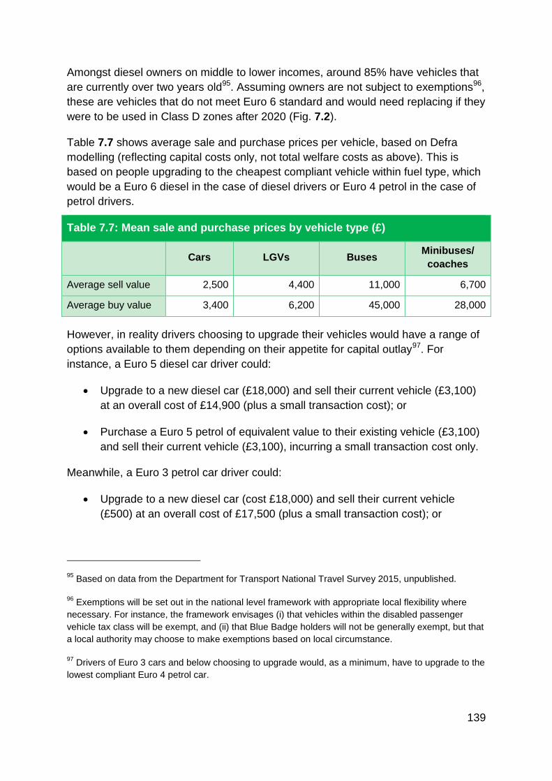
139
Amongst diesel owners on middle to lower incomes, around 85% have vehicles that
are currently over two years old95. Assuming owners are not subject to exemptions96,
these are vehicles that do not meet Euro 6 standard and would need replacing if they
were to be used in Class D zones after 2020 (Fig. 7.2).
Table 7.7 shows average sale and purchase prices per vehicle, based on Defra
modelling (reflecting capital costs only, not total welfare costs as above). This is
based on people upgrading to the cheapest compliant vehicle within fuel type, which
would be a Euro 6 diesel in the case of diesel drivers or Euro 4 petrol in the case of
petrol drivers.
Table 7.7: Mean sale and purchase prices by vehicle type (£)
Cars LGVs Buses
Minibuses/
coaches
Average sell value 2,500 4,400 11,000 6,700
Average buy value 3,400 6,200 45,000 28,000
However, in reality drivers choosing to upgrade their vehicles would have a range of
options available to them depending on their appetite for capital outlay97. For
instance, a Euro 5 diesel car driver could:
Upgrade to a new diesel car (£18,000) and sell their current vehicle (£3,100)
at an overall cost of £14,900 (plus a small transaction cost); or
Purchase a Euro 5 petrol of equivalent value to their existing vehicle (£3,100)
and sell their current vehicle (£3,100), incurring a small transaction cost only.
Meanwhile, a Euro 3 petrol car driver could:
Upgrade to a new diesel car (cost £18,000) and sell their current vehicle
(£500) at an overall cost of £17,500 (plus a small transaction cost); or
95 Based on data from the Department for Transport National Travel Survey 2015, unpublished.
96 Exemptions will be set out in the national level framework with appropriate local flexibility where
necessary. For instance, the framework envisages (i) that vehicles within the disabled passenger
vehicle tax class will be exempt, and (ii) that Blue Badge holders will not be generally exempt, but that
a local authority may choose to make exemptions based on local circumstance.
97 Drivers of Euro 3 cars and below choosing to upgrade would, as a minimum, have to upgrade to the
lowest compliant Euro 4 petrol car.

140
Purchase the oldest compliant Euro 4 petrol car on the market (cost £1,150)
and sell their current vehicle (£500) incurring an overall cost of £650 (plus a
small transaction cost).
It is also worth noting that there may be differences in running costs between petrol
and diesel cars.
The cost estimates for upgrading the fleet assume that the resale market is
unaffected by the changes to policy, allowing owners of older cars to sell them on
and buy compliant replacements at current market rate.
If owners are unable to sell their non-compliant vehicles at the assumed rate
because the market has been affected, they may be exposed to lower ‘sell’ values as
well as increases in ‘buy’ costs for an equivalent compliant vehicle. Table 7.7 gives
an idea as to the scale of risk for owners should the market be affected. However,
the initial analysis is that availability of compliant, second hand cars should remain
stable.
The numbers of cars in the 2020 fleet affected by the proposed measures are
estimated to be around 7.5 million diesel vehicles and around one million petrol
vehicles (see Annex D for more detail). Assuming c. 14% of these were replaced
(Table 4.4), around one million diesel vehicles and 140,000 petrol vehicles would be
needed (1.2 million cars in total). 20 million compliant cars are potentially available
(six million diesel and 14m petrol)98. SMMT figures show that around eight million
second-hand cars changed hands in 201699 representing around 27% of a total 2016
fleet size of 29.5 million. It would therefore be expected that a large proportion of the
potentially available compliant cars would be available for purchase in the run up to
2020 – approximately five million (25% of 20 million) per year100. This should
comfortably cover the 1.2 million needed, even taking regional differences into
account.
The overall discussion on private vehicles in Section 7.3.2 helps improve
understanding of the possible effect of CAZs on owners of private cars. However, for
a more detailed assessment of the effects of the proposed measures across the
population, a better understanding of current driving practices, vehicle use and the
98 Calculated as total number of compliant vehicles minus those affected by CAZs.
99 SMMT, Used Car Sales: Q4 2016, 15 February 2017 <https://www.smmt.co.uk/2017/02/used-car-
sales-q4-2016/>.
100 Please note, this is based on 2020 fleet sizes so the actual number available in 2017-2019 will be
slightly lower.

141
alternatives is required (for instance the ability of public transport networks to provide
a viable alternative to those currently driving the most polluting vehicles). This is
briefly discussed in Section 9.
Buses
The economic analysis of buses and coaches has assumed that the cost of
upgrading the fleet would be passed onto passengers directly over the course of a
year, on a per journey basis and excluding passengers under five and over
retirement age101.
Based on modelling undertaken with the Fleet Adjustment Model (see Section 3.3.3),
the overall cost to the fleet is estimated to be c. £270m or around £5,700 per
affected vehicle. This assumes the resale market is unaffected by the changes to
policy, allowing owners of older buses to sell these on at current market prices and
trade up to compliant ones. Averaged across the UK population aged between five
and 62/65102, this is an average per person cost of c. £5.50 and an average per
journey cost of around 9p. As those in the lowest income levels make greater use of
buses and coaches (Fig. 7.5), this translates to an average overall cost of c. £8.60
for those in the lowest income quintile and £5.90 for people on middle to lower
incomes compared with £2.90 for those in the highest income quintile.
We have not accounted for the fact that the cost of upgrades might only be passed
onto passengers using buses and coaches in particular geographic areas (areas with
CAZs or older bus fleets for example). Nor has the fact that bus usage (and
payment) is not spread evenly across the population within income quintiles. Costs
are therefore likely to be higher for fare payers who make regular use of buses in
and around CAZ areas. This said, some costs might be borne by Local Authorities
through their funding of free travel for eligible groups. Bus operators may also be
able to reassign buses and coaches in their fleet based on which buses are and are
not likely to enter CAZs to minimise costs.
101 Entitlement to free travel varies across the UK. However, children under five and those who have
reached retirement age usually travel without charge under the ‘English National Concessionary Bus
Travel Scheme’ or the ‘Freedom pass’ scheme in London.
102 These are the respective state pension ages for women and men reaching retirement age in 2015.

142
LGVs
The overall cost of scrappage and upgrades to the LGV fleet is estimated to be
around £577m and around £1,430 per affected vehicle.
Information of how ownership of LGVs is spread across socio-economic groups is
not currently held by Defra; however it is likely that those in lower income brackets
will have a greater proportion of older vehicles and, therefore, greater exposure to
the costs of replacing non-compliant vehicles.
7.3.4 Financial effects of other measures
Other measures with differentiated financial effects across socio-economic groups
have been briefly considered as follows:
Local measures
As local measures will be designed to be responsive to local needs, there is a great
deal of flexibility in how they might be used. Because of this, there cannot be any
certainty around their distributional effects across the population. However, any
moves to encourage a modal shift away from private cars are likely to have a
positive effect on lower income groups both because they may be able to benefit
from alternatives directly and because they are adversely affected by current traffic
levels. As well as suffering directly from poor air quality, as described in Section 7.2,
there is evidence those in lower income groups are more likely to be killed or
seriously injured in road traffic accidents. DfT research shows that in 2013 around
one third of people suffering such casualties lived in the 20% most deprived areas
while only 13% lived in the 20% least deprived areas103.
Retrofit
As this measure targets businesses and local authority bus fleets, there will not be
any direct effects on lower socio-economic groups. However, there may be indirect
benefits for lower socio-economic groups if retrofit funding is used to minimise the
upgrade costs passed onto passengers.
103 Department for Transport, ‘Facts on Pedestrian Casualties’ (June 2015)
<https://www.gov.uk/government/uploads/system/uploads/attachment_data/file/448036/pedestrian-
casualties-2013-data.pdf>.

143
Scrappage
As the option proposed targets the oldest vehicles, a scrappage scheme (affecting
c.15,000 vehicles, the majority of which are likely to be cars) could be very relevant
to lower income groups. However, the extent of this effect depends on exactly how
the scheme is implemented.
The option modelled in Section 5 requires scrapped vehicles to be replaced with
Battery Electric Vehicles (BEVs). As these vehicles are relatively more expensive it
might be less likely that those on lower incomes would take up this scheme.
However other designs of scrappage schemes could avoid such impacts, for
instance not including a requirement to replace with a BEV or targeting at those who
are most in need of support.
Ultra Low Emission Vehicles (ULEVs)
Extending the Plug-in Car Grant is unlikely to have a direct effect on lower income
groups, as they are less likely to purchase a new (electric) car, even with a grant
(Table 7.4).
The authors of a recent rapid evidence assessment for DfT felt that, based on
insights from more developed ultra low emission vehicle (ULEV) markets, the basic
socio-demographic profile of ULEV owners in the UK was not likely to change
substantially over the coming years. They identified this demographic as middle-
aged, male, well educated, affluent, and living in urban areas with households
containing two or more cars and with the ability to charge at home104.
The Plug-In grant is therefore likely to support more affluent households; however it
is also likely to support lower income groups by increasing availability (and reducing
costs) of second hand cars.
Speed limits
Reducing speed limits is likely to have a smaller effect on those with lower incomes
than on the population as a whole as, on average, they make fewer trips by car than
those in higher income groups (Fig. 7.5).
104 Brook Lyndhurst, ‘Uptake of Ultra Low Emission Vehicles in the UK. A Rapid Evidence
Assessment for the Department for Transport’ (2015) <http://www.brooklyndhurst.co.uk/uptake-of-
ultra-low-emission-vehicles-in-the-uk-_270?path=19,270>.

144
Government vehicles
There is no direct financial effect on the public or lower socio-economic groups given
that the scope of this measure is the Government fleet. How the policy would be
financed (and other indirect effects) has not been considered for this analysis.
Vehicle labelling
Including NOx information on labels is expected to have some effect in directing
individuals towards petrol vehicles and/or to downsize. In the short term, this would
mainly affect industrial users and higher income groups making new purchases (see
Section 7.3.2). However, in the longer term, lower income groups will be affected by
the availability of these cars on the second hand market. Individuals that travel long
distances would be disadvantaged by the higher running cost of petrol vehicles but
those who choose to downsize should see a reduction in running costs.
Influencing driving style
Efforts to influence driving style are likely to have a positive financial impact on
drivers in lower income groups, thanks to the resulting fuel savings.
It is possible that drivers in lower income groups may draw a disproportionate benefit
since indicative evidence of existing variation in driving practices across
demographics suggests well educated, affluent women (aged 25 to 65, with low
annual mileage and using a small vehicle) are currently the most likely to practise
efficient driving105.
There is a broad consensus that training for existing private drivers can lead to a
reduction in fuel use although estimates of likely reductions vary, partly due to the
range of interventions possible to influence driving style. One synthesis study quoted
savings of up to 25% immediately following training; and up to 10% in the long-
term106,107. Meanwhile, evidence from the Energy Saving Trust (2013)108 found that
most drivers could improve their fuel consumption by up to 15% in the short-term
105 Brook Lyndhurst, ‘Efficient Driving. A Rapid Evidence Assessment for the Department for
Transport’ (2016)
<https://www.gov.uk/government/uploads/system/uploads/attachment_data/file/509972/efficient-
driving-rapid-evidence-assessment.pdf>.
106 Ibid.
107 Findings on the impact of training employee drivers are similar – suggesting an immediate
reduction of up to 25%; and of up to 6.5% in the long-term.

145
when taught ‘eco-driving’ techniques. Additionally, a TNO study109 showed that in
combination with gear shift indicators (which show a driver when it is most
economical to change up a gear), eco-driver training can result in over 4% fuel
savings in the long-term.
7.4 Conclusion
Through greater exposure to NO2 and greater prevalence of underlying risk factors, it
is likely that those on lower incomes will benefit disproportionately from attempts to
reduce high concentrations of NO2. However, specific groups within these
populations, such as those who are heavily reliant on the oldest cars or who make
frequent use of buses for which they are paying directly, may also be
disproportionately affected by the cost of the proposed measures.
108
Quoted in Ricardo, ‘Evidence review on effectiveness of transport measures in reducing nitrogen dioxide’ (2016).
109 TNO (2006) quoted in Ricardo, ‘Evidence review on effectiveness of transport measures in
reducing nitrogen dioxide’ (2016).

146
8. Sensitivities and uncertainties
8.1 Introduction
Inherent with any piece of analysis is an element of uncertainty, particularly when
attempting to predict the future under a certain set of conditions (Fig. 8.1).
Understanding these potential uncertainties forms an integral part of the analysis
presented in this technical report, and in doing so supports the draft Plan by making
clear the probable variabilities which exist in the evidence regarding the
measurement and modelling of air quality, and its connected economic and health
consequences.
Figure 8.1: Uncertainty is present in analysis of both the past and the
present, and increases for projections made further into the future
Note: This graph displays an illustrative scenario. It displays the outputs of an artificial model based
on a given set of input data (solid line) with the models corresponding predictions for the future
based on a certain set of criteria (dotted line). The shaded green ranges surrounding the lines
represent the uncertainty ranges associated with the estimates produced by the model. The
uncertainty ranges surrounding the solid line are broadly similar in width, representing the
quantified uncertainties associated with the measurements of the input data that produces
variabilities in the estimate. For projected values, the uncertainty ranges gradually increase over
time, with the lighter shades of green highlighting this. Increased uncertainty for projections
represent the different levels of confidence placed on particular scenarios holding true in the future.
Modelli
ng o
utp
ut
valu
es
Time
Projected values Observed values

147
The modelling carried out to predict future air quality is extremely complex,
particularly when the impacts of the proposed policy options are incorporated into the
assessment. This section describes the key inputs and assumptions underpinning
the analysis and the effect that these may have on contributing to the uncertainty of
the results is considered.
The inputs and assumptions used in the analysis for this technical report have been
informed by the best available evidence. This evidence draws upon existing data,
results from existing studies, and expert judgement. However, the inherent
uncertainty associated with the analysis presented can be categorised broadly as:
Uncertainties in the modelling of air quality and the resulting future
predictions.
Uncertainties in the modelling of the options to improve air quality,
including their impact on public behaviours and the effectiveness of new
technologies.
Uncertainties surrounding the quantification and valuation of air quality
impacts, particularly on human health.
As recognised in Section 1.4, the treatment of uncertainties in the report will be
aligned to IPCC guidance; details of this process are set out in Section 9.1.3. Each
of these categories is considered in the following sections. Where uncertainties have
been quantified, these have been considered for the Clean Air Zone option, unless
otherwise stated.
8.2 Uncertainties in the modelling of air quality
8.2.1 Modelling prediction uncertainty
The Pollution Climate Mapping (PCM) model provides a best estimate of
concentrations of NO2 consistent with the requirements for the annual compliance
assessment but it does not provide uncertainty ranges. This is because the model
was designed to allow an assessment of regulatory compliance and cannot, in
practice, be used to provide quantified uncertainties associated with the individual
inputs and assumptions, because each run of the model takes up to three months to
complete. The primary reason for this is the large number of complex data inputs, all
of which would individually require information on uncertainty in order to propagate
overall uncertainty. Uncertainty estimates surrounding input data are also very
limited (Table 8.2).

148
Table 8.2: Description of the uncertainties surrounding key inputs of the
PCM and Streamlined PCM model
Input Associated uncertainties
Calibration of the PCM model using air
concentration measurements for pollutants
from national monitoring stations110. These
include separate calibrations for roadside
and background concentrations.
There are uncertainties surrounding the
accuracy and precision of concentration
measurement data of pollutants from
monitoring sites. This could in turn lead to
uncertainties in the calibration of the
modelled concentrations. There are
additional uncertainties introduced when
the model is calibrated to perform at
national scales, rather than conducting
calibration at local levels.
Modelled traffic flow, which includes the
Annual Average Daily Flow (AADF) from
DfT’s national traffic census. This provides
traffic counts (e.g. number of HGVs, buses,
LGVs and passenger cars), specific to each
individual road modelled.
There are uncertainties in the
measurements of traffic count (e.g. the
frequency of sampling).
Road traffic fleet composition (which refers
to the detailed composition of the fleet, that
is, the Euro standard and fuel type of the
vehicle).
Based on a range of information including
historic vehicle licensing data, Automatic
Number Plate Recognition data from around
275 ANPR cameras, fleet turnover, mileage
and age assumptions (i.e. vehicle usage
with age on the road).
Assuming the national average fleet
composition (by road type) outside
London, rather than using local fleet
composition data specific to each
individual road introduces some
uncertainty. Further, the actual number of
vehicles of each fuel type, technology type
and age mix on the road add additional
uncertainty.
The modelled traffic speed. The average speed applied in the
modelling has been based on the type of
road (30 road types) rather than locally
monitored speed measurements or data.
Speed dependent NOx emission factors
from road transport vehicles.
Uncertainties in this input arise due to the
limited availability of test data and varying
amount of data for different vehicle types.
Emission factors also contribute to the
110 Department for Environment, Food & Rural Affairs, Automatic Urban and Rural Network (AURN),
2015 <https://uk-air.defra.gov.uk/networks/network-info?view=aurn>.

149
uncertainty, particularly for future vehicle
types (e.g. Euro 6 after further Real
Driving Emissions testing) based on
expert judgement (Emisia).
Proportion of low carbon passenger cars
and LGVs with electric and hybrid electric
propulsion systems.
There are uncertainties in the figures for
the uptake of vehicles using alternative
fuel or propulsion technologies which are
based on estimates provided by DfT
Projected future activity and emissions data
from the National Atmospheric Emissions
Inventory (NAEI), including road traffic
forecasts provided by DfT and TfL, and
energy projections from BEIS.
There are inherent uncertainties
associated with predicting future activity
based on modelled data.
NOx/NO2 relationship based on the Jenkin
equation111.
General roadside and background
relationships are estimated in the
modelling, rather than reflecting location
specific complex atmospheric chemistry.
Annual average weather data. Data taken from a single monitoring
station (Met Office station at
Waddington112), assumes uniform annual
average weather across UK.
Additional uncertainties in SL-PCM
modelling versus PCM modelling.
The impact of measures on cold start
emissions, minor roads, fleet-weighted f-
NO2, and the specific impact on
background concentrations cannot be
modelled using the SL-PCM model.
For many of these inputs, a large amount of targeted research would be required in
order to quantify and reduce the associated uncertainties. However, due to the
continually evolving nature of air quality evidence and data, further research only
forms part of a bigger picture in combating uncertainty. A deeper understanding of
the wider environment of factors that interact with the air quality modelling also
needs ongoing investigation.
111 M.E. Jenkin, ‘Investigation of the NOx-dependence of oxidant partitioning at UK sites using annual
mean data 1991-201’, 2012, Atmospheric Chemistry Services, Okehampton, Devon, UK. Available
upon request.
112 Met Office, UK climate - Historic station data <http://www.metoffice.gov.uk/public/weather/climate-
historic/#?tab=climateHistoric>.

150
For instance, data on the emissions of air pollutants which are reviewed and updated
annually through the National Atmospheric Emissions Inventory form a key input to
the PCM model. These updates reflect changes in activity data across all pollutant
sources, changes to assumptions around the distribution of emissions across the UK
and updates to emissions factors. As a result, the PCM modelling incorporates the
latest assumptions around emissions from each source, to reflect the best range of
evidence available.
Section 2.1 describes the Streamlined PCM (SL-PCM) model that was used to
analyse the air quality impact of possible measures, and how it differs from the full
PCM model. Using the SL-PCM model, rather than the full PCM model, introduces
some additional uncertainty to the results of the assessment.
Testing undertaken in 2015 by Ricardo Energy & Environment allows a quantification
of this uncertainty. These tests showed that the margin of error between the PCM
and SL-PCM model assessments for a given scenario is relatively small. This
conclusion, reached by examining the impact of four Clean Air Zone (CAZ) types,
modelled both the PCM and SL-PCM models (Table 8.3). Across the four CAZ types,
the SL-PCM model primarily produced larger changes in NO2 concentrations than
the full PCM model. Differences for the mean level of NO2 concentration ranged in
the magnitude of 0.15-0.25µg/m3 across the four CAZ scenarios, highlighting the
typically small variabilities in outcomes produced by the two models.
Table 8.3: Mean and percentile differences between PCM and SL-PCM model
outputs by CAZ type for the concentration of NO2 (μg/m3)
CAZ type Class A Class B Class C Class D
Mean -0.15 -0.20 -0.25 -0.16
5th percentile -0.67 -0.71 -0.73 -0.64
25th percentile -0.18 -0.24 -0.29 -0.18
50th percentile -0.06 -0.11 -0.16 -0.09
75th percentile 0.00 -0.04 -0.08 -0.03
95th percentile 0.12 0.07 -0.02 0.14
Note: The figures presented in this table take the mean and percentiles of the concentration of NO2
arising from the full PCM model and subtracting the outputs generated by the SL-PCM model for each
CAZ type.
A further example where air quality evidence is changing are the COPERT NOx
emission factors (Section 8.1.2). Under the normal modelling process, updated
inputs are first incorporated within the PCM model, after which a version of the SL-
PCM model is developed that is fully consistent with that PCM model. Due to the

151
length of time required for a full PCM model assessment, the existing SL-PCM model
has been adjusted accordingly to take account of the updated emission factors,
without the waiting for a full PCM model run. This will reduce the differences
between current modelling and the outputs of the future PCM modelling run with
organically integrated COPERT 5 factors. However, there are still likely to be some
difference between the results provided by these two models due to the reasons
highlighted in Section 2.1 and Table 8.2.
A sensitivity analysis, showing the effect of a ±3µg/m3 estimation error in projections
from the adjusted SL-PCM model, allow an assessment of these potential
differences (Table 8.4). The table shows how the number of areas in compliance
could change through variation in the projections. It is important to note that this
sensitivity test is showing the effect of the estimation error occurring equally in each
assessment group (i.e. every one of the 43 zones modelled having a ±3µg/m3
estimation error).
Table 8.4: Number of directive compliant assessment groupings based on
whether there was an under or over-estimation of the true NO2 concentration in
2020
Assessment
grouping Total
True value
(µg/m3 above central
projection) Central
projection
True value
(µg/m3 below central
projection)
3µg/m3 2µg/m3 1µg/m3 1µg/m3 2µg/m3 3µg/m3
Zones 43 8 9 9 12 17 21 22
Local
authorities 406 297 306 317 325 334 343 353
Postal towns 748 638 645 659 670 682 692 702
Road links 9,251 8,148 8,289 8,403 8,518 8,608 8,686 8747
Note: The SL-PCM reports results by zones, local authorities, and road links. Converting the road link
outputs through reverse geocoding produces the ‘postal town’ assessment grouping.
The results show a non-linearity in the significance of over or underestimating by
zone. For example, if subsequent estimates produced by the PCM model were to be
consistently 3µg/m3 lower than the central scenario, ten further zones would become
compliant. In contrast, only four further zones would become non-compliant for
estimates 3µg/m3 above the central projection. Therefore, an upward revision of
modelled concentrations would have a notably smaller impact than a revision in the
opposite direction.
Using this analysis, an estimation of how the number of Clean Air Zones could vary
due a ±3µg/m3 estimation error in the projections (Table 8.5) was conducted. While
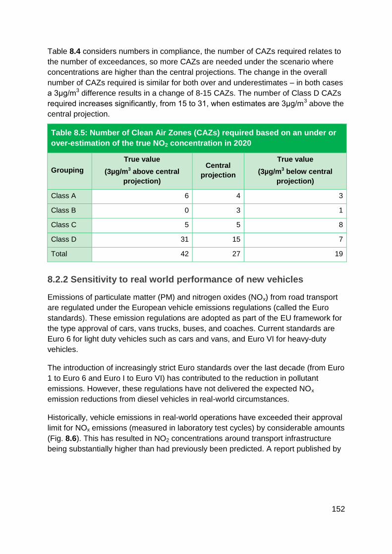
152
Table 8.4 considers numbers in compliance, the number of CAZs required relates to
the number of exceedances, so more CAZs are needed under the scenario where
concentrations are higher than the central projections. The change in the overall
number of CAZs required is similar for both over and underestimates – in both cases
a 3μg/m3 difference results in a change of 8-15 CAZs. The number of Class D CAZs
required increases significantly, from 15 to 31, when estimates are 3μg/m3 above the
central projection.
Table 8.5: Number of Clean Air Zones (CAZs) required based on an under or
over-estimation of the true NO2 concentration in 2020
Grouping
True value
(3µg/m3 above central
projection)
Central
projection
True value
(3µg/m3 below central
projection)
Class A 6 4 3
Class B 0 3 1
Class C 5 5 8
Class D 31 15 7
Total 42 27 19
8.2.2 Sensitivity to real world performance of new vehicles
Emissions of particulate matter (PM) and nitrogen oxides (NOx) from road transport
are regulated under the European vehicle emissions regulations (called the Euro
standards). These emission regulations are adopted as part of the EU framework for
the type approval of cars, vans trucks, buses, and coaches. Current standards are
Euro 6 for light duty vehicles such as cars and vans, and Euro VI for heavy-duty
vehicles.
The introduction of increasingly strict Euro standards over the last decade (from Euro
1 to Euro 6 and Euro I to Euro VI) has contributed to the reduction in pollutant
emissions. However, these regulations have not delivered the expected NOx
emission reductions from diesel vehicles in real-world circumstances.
Historically, vehicle emissions in real-world operations have exceeded their approval
limit for NOx emissions (measured in laboratory test cycles) by considerable amounts
(Fig. 8.6). This has resulted in NO2 concentrations around transport infrastructure
being substantially higher than had previously been predicted. A report published by

153
the International Council on Clean Transportation (ICCT)113 found that the
implementation of NOx control technologies by a few manufacturers resulted in some
vehicles meeting the Euro 6 limit of 0.08g/km when subjected to both the New
European Driving Cycle (NEDC), and the Worldwide Harmonized Light Vehicles Test
Cycle (WLTC)114. These results demonstrate that compliance with the Euro 6
standard is technically feasible.
On 30th September 2016 updated COPERT vehicle emission factors from Emisia
became available. The UK and a majority of other Member States use COPERT
emission factors to estimate emissions of air pollutants from road transport. This
revision, referred to as COPERT 5, provides three Euro 6 emission factors for diesel
cars and LGVs, reflecting the reduction in emission factors over time for Euro 6
diesel vehicles in response to Real Driving Emission (RDE) testing. This RDE testing
consists of two phases:
a temporary phase, Euro 6d-TEMP, with a ‘conformity factor’ of 2.1, meaning
that vehicles approved under Euro 6d-TEMP can emit 2.1 times the Euro 6
limit; and
a final phase, Euro 6d, for which the conformity factor is the margin of
uncertainty of the Portable Emissions Measurement System (PEMS)
measurement (currently 1.5).
113 The International Council on Clean Transportation (ICCT), ‘NOx control technologies for Euro 6
diesel passenger cars’, 2015 <www.theicct.org/nox-control-technologies-euro-6-diesel-passenger-
cars>.
114 The New European Driving Cycle (NEDC) serves to represent typical car usage in Europe; the
Worldwide Harmonized Light Vehicles Test Cycle (WLTC) better represents the range of real world
driving conditions.

154
Figure 8.6: Comparison of NOx (g/km) emission standards for different car
Euro classes, by emission limit and real-world performance (NOx emissions
measured in g/km)
Source: Adapted from a report by the European Environment Agency115
.
The COPERT 5 emission factors for Euro 6 used for the central analysis broadly
reflect three phases, indicating a gradual improvement in emissions due to the
effectiveness of RDE testing. They do however reflect the fact that despite
improvements in the testing procedure, there is likely to continue to be some
difference between vehicle emissions during approval testing compared to everyday
real world emissions (although this is reduced over time). While petrol cars have
performed consistently better than the Euro standard from Euro 5 onwards, diesel
cars have performed consistently worse.
115 European Environment Agency (EEA), ‘Explaining road transport emissions – A non-technical
guide’, 2016 <http://www.eea.europa.eu/publications/explaining-road-transport-emissions>.

155
Historically, more extensive emissions testing had been undertaken for older
vehicles. This is because they represent a larger fraction of the fleet and have been
in circulation longer than newer vehicles, leading to greater opportunities for testing.
Consequently, emissions from newer vehicles had larger associated uncertainties
compared to older vehicles. Since the Volkswagen emissions issue in September
2015, there has been widespread testing of Euro 6 diesel cars throughout Europe,
which has provided increased confidence in emissions from Euro 6 cars. The
greatest uncertainty is associated with future Euro 6 emissions (Euro 6d-TEMP and
Euro 6d) from diesel cars and LGVs, since evidence regarding the effectiveness of
different abatement technologies continues to evolve, and the impact of RDE
legislation is not yet known.
Given the inherent uncertainty around predicting emission factors for future vehicles,
two alternative scenarios (agreed through discussion with experts, including
representatives from Ricardo and Emisia) were modelled in addition to the central
scenario. One scenario is based on lower emissions compared to the central
scenario, whilst the other assumes higher emissions relative to the central scenario,
in order to present the possible range of likely outcomes.
The lower emissions scenario assumes that under real-world driving conditions, new
Euro 6 light duty vehicles are fully compliant with the relevant RDE legislation in
place at the time of manufacture (for both Euro 6d-TEMP and Euro 6d). The higher
emissions scenario assumes the same emission factors as COPERT 5 (which are
already considered to be cautious), but incorporates the latest possible uptake for
RDE step 1 and 2 for new vehicles permitted by the legislation. However, it should
be noted that there are already some vehicles that meet the Euro 6 standards in the
real world116.
The assumed conformity factors (scaling factors that show the number of times that
the modelled emission factors exceed the Euro 6 limit value of 0.08g/km) for light
duty vehicles, such as cars and vans, show a gradual decline in the number of times
the modelling emissions factors exceed the Euro 6 limit leading up to 2020 (Table
8.7).
116 The International Council on Clean Transportation (ICCT), ‘NOx control technologies for Euro 6
diesel passenger cars’, 2015 <www.theicct.org/nox-control-technologies-euro-6-diesel-passenger-
cars>.

156
Table 8.7: Scaled assumed factors showing the number of times that the
modelled emission factors exceed the Euro 6 limit for cars and vans
2016 2017 2018 2019 2020
Cars Q1 Q2 Q3 Q4 Q1 Q2 Q3 Q4 Q1 Q2 Q3 Q4 Q1 Q2 Q3 Q4 Q1 Q2 Q3 Q4
Central 6.7 6.7 6.7 6.7 5.1 5.1 5.1 5.1 5.1 5.1 5.1 5.1 2.5 2.5 2.5 2.5 2.5 2.5 2.5 2.5
Low 6.7 6.7 6.7 6.7 6.7 6.7 6.7 2.1 2.1 2.1 2.1 2.1 2.1 2.1 1.5 1.5 1.5 1.5 1.5 1.5
High 6.7 6.7 6.7 6.7 6.7 6.7 6.7 6.7 6.7 6.7 5.1 5.1 5.1 5.1 5.1 5.1 2.5 2.5 2.5 2.5
LGVs Q1 Q2 Q3 Q4 Q1 Q2 Q3 Q4 Q1 Q2 Q3 Q4 Q1 Q2 Q3 Q4 Q1 Q2 Q3 Q4
Central 7.6 7.6 7.6 7.6 4.0 4.0 4.0 4.0 4.0 4.0 4.0 4.0 4.0 4.0 4.0 4.0 2.0 2.0 2.0 2.0
Low 7.6 7.6 7.6 7.6 7.6 7.6 7.6 7.6 7.6 7.6 7.6 2.1 2.1 2.1 2.1 2.1 2.1 2.1 1.5 1.5
High 7.6 7.6 7.6 7.6 7.6 7.6 7.6 7.6 7.6 7.6 7.6 7.6 7.6 7.6 7.6 7.6 4.0 4.0 4.0 4.0
The impact of the high and low emissions scenarios on NOx emissions was modelled
using these conformity factors. This then allowed for a valuation of the health
benefits (Table 8.8).
Table 8.8: Sensitivity analysis on diesel Euro 6 LDV emissions and associated
impacts on benefits for Clean Air Zones
Scenario
Inside zone
emissions
change,
tonnes
Outside zone
emissions
change,
tonnes
Total NOx
benefits (£m)
Overall NPV
(£m)
Central -40,841 17,264 £3,612 £1,099
Low conformity factors -33,118 13,065 £3,280 £768
High conformity factors -43,589 18,759 £3,729 £1,216
8.3 Measure modelling uncertainties
A range of additional uncertainties exists in relation to the design of each possible
measure, which has not been possible to quantify. Many of these stem from an
absence of information on the behavioural responses that people may choose to
adopt in response to the implementation of a particular measure.
There is a large amount of uncertainty surrounding the responses of vehicle owners
to the implementation of a Clean Air Zone due to the number of potential choices
that affected vehicle operators may choose. These include avoiding the zone,
cancelling the journey, upgrading vehicle, redeploying vehicles elsewhere or
continuing into the zone. The proportions of vehicle owners responding in each way
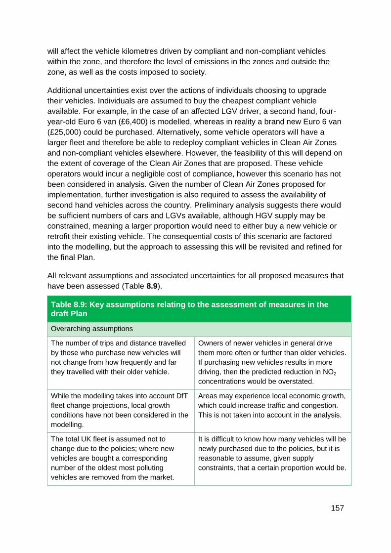
157
will affect the vehicle kilometres driven by compliant and non-compliant vehicles
within the zone, and therefore the level of emissions in the zones and outside the
zone, as well as the costs imposed to society.
Additional uncertainties exist over the actions of individuals choosing to upgrade
their vehicles. Individuals are assumed to buy the cheapest compliant vehicle
available. For example, in the case of an affected LGV driver, a second hand, four-
year-old Euro 6 van (£6,400) is modelled, whereas in reality a brand new Euro 6 van
(£25,000) could be purchased. Alternatively, some vehicle operators will have a
larger fleet and therefore be able to redeploy compliant vehicles in Clean Air Zones
and non-compliant vehicles elsewhere. However, the feasibility of this will depend on
the extent of coverage of the Clean Air Zones that are proposed. These vehicle
operators would incur a negligible cost of compliance, however this scenario has not
been considered in analysis. Given the number of Clean Air Zones proposed for
implementation, further investigation is also required to assess the availability of
second hand vehicles across the country. Preliminary analysis suggests there would
be sufficient numbers of cars and LGVs available, although HGV supply may be
constrained, meaning a larger proportion would need to either buy a new vehicle or
retrofit their existing vehicle. The consequential costs of this scenario are factored
into the modelling, but the approach to assessing this will be revisited and refined for
the final Plan.
All relevant assumptions and associated uncertainties for all proposed measures that
have been assessed (Table 8.9).
Table 8.9: Key assumptions relating to the assessment of measures in the draft Plan
Overarching assumptions
The number of trips and distance travelled
by those who purchase new vehicles will
not change from how frequently and far
they travelled with their older vehicle.
Owners of newer vehicles in general drive
them more often or further than older vehicles.
If purchasing new vehicles results in more
driving, then the predicted reduction in NO2
concentrations would be overstated.
While the modelling takes into account DfT
fleet change projections, local growth
conditions have not been considered in the
modelling.
Areas may experience local economic growth,
which could increase traffic and congestion.
This is not taken into account in the analysis.
The total UK fleet is assumed not to
change due to the policies; where new
vehicles are bought a corresponding
number of the oldest most polluting
vehicles are removed from the market.
It is difficult to know how many vehicles will be
newly purchased due to the policies, but it is
reasonable to assume, given supply
constraints, that a certain proportion would be.

158
Unless stated otherwise, people will act to
minimise financial costs. Thus, they will
decide upon the action that fulfils their
objectives at minimum cost, buying the
cheapest CAZ compliant vehicle as an
example.
In reality, people do not always make the
financially optimal decision, meaning they
might not have bought the cheapest vehicle
for their aims. Thus, some will choose to
spend more. It is also possible that some
people will not be able to act in a financially
optimal way either because they do not have
sufficient money to cover upfront costs or
because they are unable to borrow money to
cover these costs. However, it has not been
possible to quantify this.
Unless stated otherwise, the administration
and start-up costs of a policy are zero.
In reality, there are often sizeable costs in
both setting-up and administering a policy.
However, because many of the proposed
measures are simply expansions or variations
on existing ones, much of these costs have
already been taken into account.
Clean Air Zones
Assumption Associated uncertainty
The assumption for the behavioural
responses of vehicle owners is based on
an assessment of the number of vehicles
available and one previous study on
individual and business responses in
London.
London is not representative of the rest of the
UK, and therefore depending on how people
and businesses behave in response to
measures, there could be a larger or smaller
change in NOx emissions compared to the
modelling predictions.
The Clean Air Zone delivers an 80-95%
reduction in the distance travelled within
the zone by non-compliant coaches, HGVs,
LGVs and cars; and a 100 percent
reduction in those of buses. However, it is
assumed that all lost business activity is
replaced by compliant business activity.
In reality, there may be a higher or lower
proportion of non-compliant vehicles that
continue to enter the Clean Air Zone. This
would alter the estimated reduction in
emissions although it is not possible to assess
the direction or scale. There will be a larger
proportional impact on vehicle kilometres than
unique vehicles that change behaviour, given
those that upgrade are more likely to be
frequent entrants of the zones.
The analysis presented here considers the
access restriction element of Clean Air
Zones only. Other elements such as
accelerating uptake of ULEVs, raising
awareness, encouraging active travel, and
improving public transport services are not
quantified.
There are a large number of additional
measures in the national overview and zone
plan documents that are already planned by
local authorities that could not be modelled but
could be expected to lead to greater NOx
reductions than shown in the analysis, as well
as possible additional costs.

159
The modelling assumes the profile of
ownership length data, from DfT, will be
equally represented by the vehicles
affected by the Clean Air Zones.
The profile of ownership length may be longer
or shorter.
DfT GPS journey information has been
used to identify the number of unique
vehicles that are likely to enter different
networks of Clean Air Zones. This tracks a
sample of around 160,000 vehicles
travelling around the UK, and identifies
where they enter multiple cities. This
dataset has been combined with data from
the London LEZ, which identifies the total
number of unique vehicles entering London
in a year.
The sample of vehicles in the GPS sample is
not derived statistically, and may be biased
towards newer vehicles. Therefore, the
sample may overestimate the number of
unique vehicles entering Clean Air Zones.
Reduced vehicle numbers entering Clean Air
Zones would reduce costs of measures
compared with the calculations.
Robust fuel consumption data is only
available for cars and diesel LGVs. This
has been adjusted for a factor reflecting the
difference in real world and test cycle
emissions. There is no data available for
other vehicle types so it is assumed that
there are no improvements in fuel efficiency
for these vehicles.
We expect that newer vehicles other than cars
and LGVs experience greater improvements
in fuel efficiency and savings in CO2.
Therefore, there may be additional
unquantified CO2 benefits.
Zone perimeter lengths were estimated for
Nottingham, Southampton, Derby, Leeds,
and Birmingham for the 2015 Plan. The
average of these five cities has been
calculated and this is assumed to be the
perimeter length of an average Clean Air
Zone.
Until a full run of the PCM has been
completed, the exact areas of non-
compliance cannot be determined. These will
be obtained and indicative perimeters will feed
into the analysis for the final Plan. Actual
perimeters for CAZs will be determined
through feasibility studies conducted by Local
Authorities longer term.
The second hand value of vehicles is
based upon depreciation rates of the most
popular cars and vans.
The actual depreciation rates of vehicles is
uncertain, making the cost of second hand
vehicles uncertain. More or fewer second
hand vehicles may be bought than expected.
The implementation of Clean Air Zones is
assumed not to lead to vehicles owned by
businesses cancelling journeys.
Controls on the cost of the transportation of
goods could have unforeseen effects on
supply. At the same time, the wider benefits
for business from being located in a healthier,
more attractive city (for example in terms of
attraction and retention of staff, reductions in
sickness levels, etc.) have also not been
quantified.

160
In the modelling, setup costs are to be
spent in the earliest year the zones are
expected to be operational (2020) and
discounted to 2017 prices - £270m in
present value.
In reality, much of the capital expenditure will
happen prior to zones being operational;
however, this simplification has been made for
modelling the appraisal period 2020-2029.
25% of vehicles that are upgraded will be
bought new.
A 25% figure was selected via engagement
with experts involved in the implementation of
other schemes, and agreement that it was a
reasonable assumption to make. However, it
is worth noting that no empirical evidence
exists as to how large this proportion will be.
It is assumed that all CAZs will be
implemented in 2020.
In reality implementation make take longer or
shorter than anticipated and it is likely that
CAZs will not all be implemented at the same
time. Implementation dates will be determined
at a local level by local feasibility studies. If
implementation dates are different to those
modelled, the costs and benefits are likely to
change together meaning that the net impact
will be broadly the same.
Retrofit
Assumption Associated uncertainty
Market capacity is sufficient to deliver the
level of retrofit modelled.
Retrofit for buses are well established.
However, retrofit for HGVs remains unproven.
Retrofit for taxis has been undertaken to date,
but there is uncertainty about what scale can
be delivered.
Scrappage
Assumption Associated uncertainty
The grant levels are sufficiently high to:
Incentivise vehicle owners to scrap their
vehicles earlier than they otherwise would
have done; and
Incentivise these vehicle owners to
participate in the scheme to buy new
vehicles instead of used vehicles; and/or
Incentivise around 15,000 Euro 1-5
diesel/Euro 1-3 petrol car owners to buy a
battery electric vehicle if in addition to the
£2,000 grant they are also offered an
additional incentive of £6,000.
It has not been possible to quantify the
premium that vehicle owners are likely to need
(over and above the residual asset value of
their vehicle) to incentivise them to change
their behaviour (scrap their car, buy a new car
and/or buy a BEV). This could mean uptake of
the scheme would be higher or lower than
assumed and consequently the cost to
government could be higher or lower than
currently estimated.
The key associated uncertainties are the
estimated residual values, the premium

161
needed for the behaviour change, and take-up
rates for the scheme.
The analysis presented in this report has
focused on the first order effects of the
policies (i.e. no behaviour change has been
assumed)
The assessment has not taken into account
possible rebound effects such as the potential
increase in vehicle mileage (as a result of
increased fuel efficiency) which could offset
the emissions savings that have been
estimated
Ultra Low Emission Vehicles (ULEVs)
Assumption Associated uncertainty
The criteria and grant levels of the current
scheme continue to apply. So the average
grant size is £3,500 and the additional cost
of purchasing an ULEV is £9,400
In reality, the grant size and additional cost of
an ULEV will vary and is dependent on
individual vehicle specifications.
The whole of the funding pot is used to
finance ultra-low emission cars
An assumption made to simplify the modelling.
In reality, a small part of the grant will fund a
switch to ultra-low emission vans/motorcycles,
which have a different emissions profile.
Around 50% of purchases, in the central
scenario, would have occurred in the
baseline and as such would have no
additional benefits.
The baseline profile of ULEV take up may
differ from this assumption.
New ULEV purchases would come equally
from consumers switching from a new
conventional Euro 6 car, split equally
between petrol and diesel
Due to the cost differential, it is logical to
assume consumers would not be incentivised
to replace their current vehicle earlier than
they otherwise would have.
The behavioural differences this policy would
trigger among current diesel and petrol
owners have not been fully assessed.
The average price difference between an
ULEV and conventional car is larger than
the size of the grant and will remain the
same over the 10 year modelling period
The current cost of an electric or hybrid
vehicle is higher than a comparable
conventional car but overtime this cost
differential may fall.
Because the existing scheme is in place,
this scheme could be extended without lags
In reality, there may be a small administration
lag, which has not been modelled.
The scheme will be complete by 2020 and
take-up will increase linearly
The purchase of additional ULEVs through
this scheme is assumed to increase at a linear
rate, with a smaller uptake in the first year
compared to the last. By 2020, this additional
uptake is assumed to be complete.

162
Consumers are rational, so will only
purchase an EV if the additional cost of the
vehicle is less than the additional benefit of
the car
The consumer’s choice of purchasing an
ULEV is assumed to be rational. As such, they
would only purchase an ULEV if the benefit
they obtain from this consumption is equal or
higher than the cost they must incur.
Costs of charging and benefits lower noise
pollution have not been quantified and are
set to zero
These two factors will largely work to cancel
each other out, thus the effect on the
estimates would be negligible
The purchaser of an ULEV will drive it
similar to the average driver, i.e. urban/rural
drivers are equally likely to purchase an
ULEV
Modelling is based on the national average. In
reality, there may be a regional or area type
difference in the purchase of ULEVs.
The effect of signalling is ignored This assessment does not take into account
the signalling impact of increased ULEV
uptake
Speed limits
Assumption Associated uncertainty
The effect of reducing the speed limit from
70mph to 60mph can be simulated by
modelling a reduction in the average speed
(by 10 mph) on those stretches of
motorway that are failing (and have
average speeds at or close to 70mph).
The analysis is based on average modelled
speeds on the types of motorways affected. It
takes account of where average speeds are
already below 70mph. However, it is possible
that failing motorway links tend to be busier
and more congested, and therefore speeds on
them lower than average (so the impact of
lowering speed limits on these links will be
lower). The analysis does take account of
vehicles like HGVs that are already limited to
60mph or below and road links of a type with
average speeds well below 70mph.
Effects to flow of traffic have not been
considered for the analysis of speed limit
reduction.
As flow could be projected to increase or
decrease during a reduction of speed, no
adjustment in flow was accounted for. A
reduction in speed can aid transport to flow at
a steady speed, but can also decrease flow
due to travelling at a lower speed or
increasing congestion. There is uncertainty in
this area, as speed limits have not previously
been used for air quality management
purposes on the SRN. Highways England has
a range of preliminary evidence, which shows
that, in fact, NOx emissions may not reduce in
the way that the SL-PCM modelling suggests

163
if reduced speed limits were to be employed.
This evidence is subject to quality assurance
and further consideration. The evidence would
benefit from further monitoring in real world
conditions, for example at sites where variable
speed limits are used already for traffic
smoothing purposes, to understand better the
extent of the impact any change to speed
limits might have on air quality.
Government Buying Standards
Assumption Associated uncertainty
Real on the road (ORR) price117 difference
between cars bought in baseline and as a
result of the measure does not change over
the appraisal period.
Lower demand for diesel from updating GBS
might lead the price to fall and ORR price
difference to change, thus the capital
switching cost will be too low.
CO2 emissions differential between cars
bought in baseline and as a result of the
measure do not change over the appraisal
period.
Technology change may lead to an increased
proportional reduction in CO2 emissions of one
fuel over the other. This will then factor into
the cost or benefit of these emissions.
Average annual distance driven (by cars
within public sector fleet, and when the
vehicles are sold on the second hand
market) does not change over the appraisal
period
Unknown factors might influence the amount
of miles driven, which will affect running costs
and both CO2 and NOx emissions. Further, a
change in miles driven may have a greater
effect dependent on the sector, since
government may drive more (less) than the
average member of public.
Size of central government fleet does not
change over the appraisal period
Variation will affect the number of new
vehicles purchased annually and so the
magnitude of impacts.
Company car fleet assumptions are based
on information received from CCS.
Variation in the size of the fleet will have
impacts on our calculations for both the
number of vehicles purchased annually and
average distance driven. This would impact on
estimates of the policy’s costs and resulting
changes in CO2 and NOx
The impact of the GBS for central In reality, the timing has not been finalised and
could change, thus the policy might have a
117 On the road (ORR) price is the recommended retail price plus the delivery charge, plus the cost of
half a tank of fuel, the car’s number plates, road tax, and the first registration fee.

164
government begins at the start of 2018. slightly different effect. However, as the
effects are not that large and the variation in
start time is unlikely to be over 6 months in
either direction, the uncertainty is small.
The GBS contains 3 car segments, with the
following vehicles chosen as
‘representative’ of the average car in each
segment.
Segment A: Fiat 500
Petrol: 500 Pop Star 0.9 Twinair 85HP
Turbo Dualogic
Diesel: 500 Pop Star 1.3 Multijet 95hp
Segment B: Ford Fiesta
Petrol: 1.0T Eco Boost 100 PS
Diesel: 1.5 TCDi 75PS
Segment C: Ford Focus
Petrol: 1.0T Eco Boost 100PS 26
Diesel: 1.5 TCDi 95 PS S6
In reality, there are a multitude of vehicles
each with varying engine specifications and
consequently CO2 emissions. The vehicles
modelled are merely representative examples
and so both vehicle cost and CO2 saving will
depend on exactly which vehicle is chosen.
Vehicle labelling
Assumption Associated uncertainty
Any switching that occurs as a result of this
measure will be from diesel to petrol
ULEVs have the best performance in terms of
NOx emissions, so labelling may encourage
some to buy EVs. However, given that EVs
already perform well on CO2 labelling, the
switch will be marginal.
Influencing driving style
Assumption Associated uncertainty
Cars are driven by one person. Thus, the
number of cars impacted is the same as
the number of individuals receiving training.
Not everyone drives one car. Some people
share their car with other drivers whilst others
drive multiple vehicles. Thus, the modelling
may over- or under-estimate reality.
Drivers of ‘other vehicles’ (not cars or
LGVS) also drive either a car or LGV. Thus,
improvements caused by training car or
LGV drivers carry across to other vehicles
proportionally (55 cars/LGVs to each “other
vehicle”).
In reality, this proportion is unknown and there
is no certainty that the improvements in driving
style for one vehicle class translate to those in
another. Thus, the modelling might under or
over predict the spill over benefits of the
course.
The average cost of an eco-driving course
and a telematics device totals £150 and
The government increasing demand for eco-
driving courses would raise the price of the

165
that this price remains constant over the
appraisal period.
course. If government agrees a contract each
year then this will increase the cost.
A percentage reduction in fuel usage
equates to an equal percentage reduction
in NOx emissions.
The vehicles being targeted will range across
different categories, Euro standards, and
engine sizes. Thus, it is quite likely that the
relationship between fuel consumption and
NOx emissions will vary. Thus, a % reduction
fuel consumption may not lead to an equal %
reduction in NOx emissions.
8.4 Uncertainties in quantifying and valuing air quality impacts
8.4.1 Introduction
An element of uncertainty with the modelling stems from identifying and assessing
the air quality impacts of any proposed measure to control air quality. Much of this
uncertainty relates to the potential health impacts to the public that originate from
NO2 exposure, which can be made difficult to quantify as the isolation of the effects
of NO2 from other air pollutants is not always clear. A range of additional impacts
also results from air pollution, such as worker productivity and harm to natural
ecosystems, which also require attention in order to fully grasp the full extent of air
quality impacts.
8.4.2 Sensitivity on health impacts of NO2 exposure
The quantification of health impacts (Section 3.3.2) is based on epidemiological
studies that investigate statistical associations between NO2 concentrations and
mortality risk. Such studies usually use outdoor air pollution concentrations at the
residential addresses as a proxy for personal exposure to NO2.
The Committee on the Medical Effects of Air Pollutants (COMEAP) has noted that
there is no clear evidence for a threshold effect118 from exposure to NO2. Therefore,
during the modelling it has been assumed that mortality changes in a linear manner
with changes in NO2 concentrations. The impact on the analysis in this report, were
a threshold to be present, is expected be minimal as the reduction in concentrations
through the measures is focused on populations with higher levels of exposure.
118 A threshold effect is a dose or exposure concentration below which a defined effect will not occur.

166
To reflect the range of current evidence of the mortality effect associated with NO2
concentrations, the central risk coefficient (2.5%) has been compared against the
range of risk coefficients as recommended by COMEAP (1% and 4%). Using
COMEAP’s lowest risk coefficient of 1%, the benefits of reducing NO2 are 40% lower
than the central estimate. In contrast, the maximum risk coefficient leads to
estimated benefits that are 60% higher than the central estimate (Table 8.10).
Table 8.10: Monetised health benefits of NO2 reduction from Clean Air
Zones
Scenario NO2 health benefit (£m) NPV (£m)
Central risk coefficient
(2.5%)
3,611.5 1,098.8
High-risk coefficient (4%) 5,778.4 3,265.7
Low risk coefficient (1%) 1,444.6 -1,068.1
Importantly there is also uncertainty in assessing the mortality impacts of policies
that primarily reduce NO2 concentrations, compared with actions that reduce the
whole mix of air pollutants. This is because of the uncertainty, noted by COMEAP119,
about the extent to which NO2 itself is responsible for the associations with mortality
reported in epidemiological studies. These issues have been discussed by COMEAP
a number of times since the interim advice was provided. A decision on how the
question of causality could be addressed quantitatively is still in development.
However, from the current discussions, it appears likely that this may considerably
reduce the coefficient recommended for assessing the benefits of measures that
would primarily reduce NOx emissions alone.
There is likely to be substantial overlap if effects are estimated on the basis of both
NO2 and PM2.5 concentrations when coefficients from single-pollutant models are
used in the same analysis. To avoid this risk only the impact of NO2 concentrations
has been valued.
COMEAP has noted that uncertainty still remains around the potential overlap
between the health effects found in epidemiological studies to be associated with PM
and NO2. They previously suggested reducing the NO2 coefficient by 33% to take
account of double counting of effects associated with PM, but have noted that
119 Committee On The Medical Effects of Air Pollutants (COMEAP), ‘Interim statement on quantifying
the association of long-term average concentrations of nitrogen dioxide and mortality’, 2015
<www.gov.uk/government/uploads/system/uploads/attachment_data/file/485373/COMEAP_NO2_Mor
tality_Interim_Statement.pdf>.

167
uncertainty around the magnitude of this adjustment still exists120. Nevertheless, it
should be recognised that COMEAP advice is evolving in response to current
scientific evidence and changes will have implications for the cost benefit analysis.
8.4.3 Sensitivity on NOx damage cost
Damage costs provide a coherent way to value changes in air pollution. They seek to
estimate the cost to society of a change in the emission of a given pollutant. They
can be provided by pollutant, source, as well as location. However, damage costs
are only as good as the information used to derive them. Defra is currently updating
its damage costs to account for new information, which includes updating the NOx
damage costs and the dispersion modelling underlying this. In the current published
damage costs, the emission to concentration relationships for NOx emissions to NO2
concentrations was assumed to be equivalent to the relationship between PM2.5
emissions and PM2.5 concentrations. However, in light of new information, revisions
to the latest dispersion modelling will ultimately lead to a better representation of the
costs of air pollution to society.
Sensitivity on morbidity impacts
The change in mortality associated with exposure to NO2 concentrations has been
valued in the economic assessment. However, other costs such as short-term health
impacts on hospital admissions and other health care costs have not been assessed.
This is likely to lead to an underestimate of the benefits of reducing NO2
concentrations.
A quantified sensitivity analysis has been conducted on bronchitic symptoms in
asthmatic children and respiratory hospital admissions using World Health
Organization guidance121. The expected reduction in costs associated with these
types of admissions because of a reduction in NO2 concentration is expected to be in
the region of £38m. However, this estimate does not capture the impacts on a wide
range of additional morbidity impacts, which have not been possible to quantify, but
are likely to be influential.
120 Ibid.
121 World Health Organization, ‘Health risks of air pollution in Europe – HRAPIE project.
Recommendations for concentration–response functions for cost–benefit analysis of particulate
matter, ozone and nitrogen dioxide.’ (2013)
<http://www.euro.who.int/__data/assets/pdf_file/0006/238956/Health-risks-of-air-pollution-in-Europe-
HRAPIE-project,-Recommendations-for-concentrationresponse-functions-for-costbenefit-analysis-of-
particulate-matter,-ozone-and-nitrogen-dioxide.pdf?ua=1>.

168
A report, published by the Royal College of Physicians in 2016122, outlined the
impacts of air pollution on health. It found that air pollution, including NO2, is linked
with a number of morbidity impacts, which have not been valued in the analysis
presented in this report. In addition to respiratory problems and reduced lung
function, these also include damage to neurodevelopment, cognitive function, and
cardiovascular disease.
8.4.4 Other air quality impacts
Productivity
Air pollution has an impact on morbidity; both the amount of time people physically
are at work and through their efficiency while working. There may also be additional
impacts on mortality and morbidity in non-market productive activities such as
volunteering and non-paid caring. It has not been possible to quantify the reduction
of these impacts, but it is likely the benefits will be significant. Defra has
commissioned work considering the links between air quality and productivity123 and
identified a number of relevant impact pathways. However due to the uncertainties
surrounding the pathways quantification of these has not been incorporated into the
central guidance on quantification.
Ecosystem services
Air pollution has considerable impact on the natural environment via processes such
as eutrophication of terrestrial and aquatic ecosystems, acidification of soils and
freshwaters, and direct toxicity effects of ground level ozone. These ecological
impacts affect supporting ecosystem services, with a large number of consequential
effects. Defra has commissioned work considering the impacts on ecosystems of
pollution124. However, as with productivity impacts, given the uncertainty over the
122 Royal College of Physicians, ‘Every breath we take: the lifelong impact of air pollution’, 2016
<https://www.rcplondon.ac.uk/projects/outputs/every-breath-we-take-lifelong-impact-air-pollution>.
123 Ricardo-AEA, ‘Valuing the Impacts of Air Quality on Productivity’, Final Report for the Department
for Environment, Food & Rural Affairs, 2014 <https://uk-
air.defra.gov.uk/assets/documents/reports/cat19/1511251135_140610_Valuing_the_impacts_of_air_q
uality_on_productivity>.
124 Centre for Ecology and Hydrology (CEH), ‘Using the Ecosystems Services Approach to Value Air
Quality’, Report for the Department for Environment, Food & Rural Affairs, 2012 <https://uk-
air.defra.gov.uk/assets/documents/reports/cat10/1511251138_NE0117_Using_the_ecosystems_servi
ces_approach_to_value_air_quality.pdf>.
169
magnitude of these impacts they have not been incorporated into the central
guidance on quantification.
8.5 Discussion
Acknowledging the inevitable uncertainties with the modelling and its associated
risks forms an important in step in understanding the relative strengths and
weaknesses of the approach taken to measure the impacts of any proposed
measure and in doing so supports the decision-making process. Throughout the
analysis, the best possible data sources, evidence and expert judgement
surrounding both the modelling of air quality and its connected health and economic
consequences have been utilised, thus providing a solid foundation for the results
produced.
In many cases, a number of assumptions have been employed and an assessment
into the robustness of these assumptions allows an identification of the true
limitations of the current data (Table 8.9). Within this assessment, it is evident that
there is a certain degree of ‘noise’ present with the data used to inform the analysis
of intervention measures. These are small amounts of error that can occur naturally
on all data points in every dimension (e.g. variations in the precision of
measurements, rounding or having other background data that is indistinguishable
from the actual data being measured), but generally have little effect when evidence
is analysed. Thus, the existence of noise and adjustments to individual parameters
do not drive fundamental changes in outcomes and consequently allows confidence
to be placed in the processes and analysis presented in this report.
The inherent uncertainties surrounding the analysis does not present reason for
inaction, but rather motivation to continually develop knowledge, evidence and
monitoring of air quality so that an increasing high-quality evidence base can be
achieved. In doing so, uncertainties can be reduced in a multi-faceted way, thus
incrementally building confidence in the way intervention measures can be
effectively implemented. The steps that are required to attain this goal are addressed
in Section 9.

170
9. Future steps
This section describes the longer-term plan to improve air quality, covering:
Developing the final Plan following this consultation
Evidence requirements for implementation and evaluation of the final Plan
Plans to further improve the evidence in the longer term
Developing an air quality strategy
9.1 Developing the final Plan
The work required to move from the analysis presented in this report to that in the
final Plan will include:
Incorporating consultation responses
Conducting a full analysis of the final Plan
Improving the quantification of expression of uncertainties
An overview of the plan for this process is illustrated by Figure 9.1.

171
Figure 9.1: A flow chart to illustrate the process of transitioning from consultation
to the final analysis

172
9.1.1 Incorporating consultation responses
Responses to this consultation may lead to changes in the assessment methods or
the measures that are assessed. These changes will be described in detail in the
final technical report and reasons for change will be incorporated.
9.1.2 Full analysis of the final Plan
The next stage of the process will be to identify and assess the package of
measures that will form the final Plan. Given the time required to complete this
analysis it will be necessary to use a modular approach. This approach is formed of
four parts:
PCM modelling
Updating the SL-PCM model
Package analysis – air quality impacts
Package analysis – option assessment
PCM modelling
The Pollution Climate Mapping (PCM) model is described in detail in Section 2.1.
The model requires the collation of a wide range of inputs across different source
sectors to make air quality projections. The complexity of the PCM model means that
significant set-up, processing, computation and quality assurance is required, with
the model taking around three months to run scenarios once the policies to be
assessed have been agreed. Steps to improve this situation are considered in
Section 9.3.
To provide the most up to date assessment of the expected future compliance
challenge, updated baseline projections from a base year of 2015 are currently being
calculated using the PCM model for every year from 2017-2030 inclusive.
These projections will be the basis for the final Plan and will reflect the latest
evidence around road transport emission factors (COPERT 5) and road traffic
projections, and will be based on the latest available base year (2015).
Updating the modelling in this way means there will be some differences in the
evidence base used for the consultation and final Plan. However, these differences
should primarily arise in the detail, rather than significantly changing the scale of the
challenge.
173
Updating the SL-PCM model
To enable more flexible assessments, a simplified version of the full PCM model,
known as the Streamlined PCM (SL-PCM) model, has been developed. This was
also used to model a small number of measures in the ‘Air quality plan for nitrogen
dioxide (NO2) in UK (2015)’.
The SL-PCM model is based on the PCM model but incorporates some
simplifications which together substantially reduce the modelling time thereby
allowing assessments of policies under multiple scenarios (see Section 2.1 for more
details).
The routine process for updating the SL-PCM model involves first calculating the
PCM modelled projections, and then building a SL-PCM model that is fully consistent
with that PCM assessment. For this draft Plan there was not sufficient time to update
the PCM projections first and then develop a new SL-PCM model for assessment of
measures. As such, the baseline projections and analysis of measures presented in
the draft Plan for consultation were derived using a previous version of the SL-PCM
model. The version of SL-PCM model used for this report projects concentrations
from the 2013 base year (2013-SL-PCM), but has been updated as far as possible
(e.g. including September 2016 COPERT 5 NOx emission factors, and using the
latest model calibration against the measurement data).
The analysis for the final Plan will be undertaken using an updated version of the SL-
PCM model that is fully consistent with the updated PCM modelling using the latest
evidence and 2015 base year (2015-SL-PCM). The differences arising between the
projections provided by the 2013-SL-PCM model and the 2015-SL-PCM model
should not hinder consultees’ ability to respond now. It is not expected that the
overall scale of the challenge will change significantly although there will be
differences in the detail (e.g. specific concentrations on individual roads or detailed
source apportionment).
Package analysis – air quality impacts
The new 2015-SL-PCM will be used to assess the impact of the final package of
measures for the final Plan. As part of this assessment, the following scenarios will
be modelled:
National type A CAZ (in 2018-2025 & 2030)
National type B CAZ (in 2018-2025 & 2030)
National type C CAZ (in 2018-2025 & 2030)
National type D CAZ (in 2018-2025 & 2030)

174
Bringing together the modelling from these different scenarios will provide an
assessment of the impact of CAZs of different stringency in different areas.
As well as the additional scaling of CAZs a number of other measures are likely to
need to be assessed. This package of measures will not be defined until the
consultation has been concluded and the responses assessed.
This model will take the agreed CAZ implementation as the baseline and then make
changes to the fleet as appropriate to reflect the wider measures. This will be done in
line with the methodology set out in Section 2.1.
Package analysis – option assessment
Finally, the package of measures will be assessed with the methods described in
Section 3.3 to understand its full impact on society including health, the economy,
and the distribution of impacts on different groups. This analysis will take account of
emerging advice on health impacts (Section 8.4.2) and any early findings from
ongoing work to improve the accuracy of distributional analysis (Section 9.3.2).
9.1.3 Improving the expression of uncertainty
A particular area of development recommended by the Air Quality Review Group
(Annex F) before production of the final Plan is the consideration and presentation of
the broad range of uncertainties that affect it. As stated earlier in Sections 1.4 and
8.1, work is ongoing to assess the uncertainties using IPCC guidance on calibrated
uncertainty language125 126.
Defra will look to convene a panel of relevant experts with the aim of providing an
independent expert assessment of the degree of uncertainty in our analysis. This will
be presented in the final Plan following the IPCC recommended approach.
The assessment can be conducted using two methods:
A qualitative assessment of the confidence of the validity of a given finding
125 Mastrandrea, M.D. et al., ‘Guidance Note for Lead Authors of the IPCC Fifth Assessment Report
on Consistent Treatment of Uncertainties’ (2010) Intergovernmental Panel on Climate Change
<https://www.ipcc.ch/pdf/supporting-material/uncertainty-guidance-note.pdf>.
126 Mastrandrea, M.D. et al., ‘The IPCC AR5 guidance note on consistent treatment of uncertainties: a
common approach across the working groups’, Climatic Change 108: 675 (2011)
<http://link.springer.com/article/10.1007/s10584-011-0178-6>.

175
A quantified, probabilistically-expressed measure of the uncertainty, based on
analysis
The decision on which method to use will be made based on the nature of the
evidence that is being evaluated (see Annex E for more detail).
Qualitative assessment
IPCC guidance recommends that for qualitative assessments, expert judgements are
used to evaluate key findings and that transparent accounts are maintained of the
process followed in coming to the judgements.
Judgements of confidence follow two ways of assessing validity:
‘Evidence’ statements based on type, amount, quality, and consistency (using
the summary terms “limited,” “medium,” or “robust”)
The degree of ‘agreement’ (using the summary terms: “low,” “medium,” or
“high”).
A level of confidence is then expressed using the qualifiers ‘very high’, ‘high’,
‘medium’, ‘low’ and ‘very low’, which synthesises these evidence and agreement
statements (Fig. 9.2).

176
Figure 9.2: Evidence and agreement statements and their relationship to
confidence127
Note: Confidence increases towards the top-right corner as suggested by the increasing strength of
shading. Generally, evidence is most robust when there are multiple, consistent independent lines of
high-quality evidence.
Quantitative assessment
For quantitative assessments, the IPCC guidance recommends that a probabilistic
estimate of the occurrence of a single event or outcome is produced, using the
measures of likelihood defined in Table 9.3.
127 Mastrandrea, M.D. et al., ‘Guidance Note for Lead Authors of the IPCC Fifth Assessment Report
on Consistent Treatment of Uncertainties.’ (2010) Intergovernmental Panel on Climate Change
<https://www.ipcc.ch/pdf/supporting-material/uncertainty-guidance-note.pdf>.

177
Table 9.3: Likelihood terms associated with outcomes used by the
IPCC128
Term Likelihood of the outcome
Virtually certain 99–100% probability
Very likely 90–100% probability
Likely 66–100% probability
About as likely as not 33–66% probability
Unlikely 0–33% probability
Very unlikely 0–10% probability
Exceptionally unlikely 0–1% probability
Note: Additional terms (extremely likely: 95–100% probability, more likely than not:
>50–100% probability, and extremely unlikely: 0–5% probability) may also be used
when appropriate.
9.2 Evaluation of the final Plan
Given the uncertainties in the evidence on the impacts of the proposed measures
(Section 8), it will be important to use an adaptive approach to implementation
whereby the impact of the measures is monitored and they are adjusted as
necessary based on emerging evidence.
By adopting this flexible approach to implementation, and integrating robust
measurement and evaluation of the performance of these interventions to control air
quality, measures can be adjusted in a way that builds on an improving evidence
base. In this way, the final Plan will be able to respond to any uncertainty in a
constructive manner and so incrementally build confidence in which methods are
most effective and drive continuous improvement.
Ongoing implementation of the measures in the UK Air Quality Plan for tackling
nitrogen dioxide published in 2015 is a useful learning opportunity providing lessons
that can feed into the delivery of the final Plan. For example, the guidance given to
local authorities implementing CAZs will be refined based on feedback and their
128 Ibid.

178
experiences of conducting feasibility studies can provide useful lessons and
information for any further feasibility studies required in the final Plan129.
To ensure the right evidence is available to use an adaptive management approach
to the implementation of these policies, consideration is being given to:
The design of proportionate evaluation processes that will measure the
impacts of the measures in the final Plan and compare them to ‘control areas’
where there have been no interventions.
Setting up appropriate monitoring and data collection processes
Conducting feasibility studies in cities that are implementing CAZs to improve
evidence on a local level and increase confidence that the design of the zone
is correct to deliver the desired impact.
Ensuring robust appraisals of any local measure or retrofit funding to allow for
evaluation of associated air quality, health and economic consequences
Addtional evaluation of data collected, widening the evidence base for
measures that work effectively with regards to improving air quality.
Adaptation of national and local measures to optimise the range of policy
interventions in use.
The detail of this process will depend on the makeup of the final Plan but it is
anticipated that a high level of evidence and resource will be required because air
quality is high profile and the policies are expected to have wide-ranging
environmental, economic, and social impacts.
Data collection by local authorities with CAZs, along with appropriate data about
other national policies, will be integral to assessing the success of different
interventions to control air quality. Consideration will be given as to whether sufficient
value will be obtained from commissioning an evaluation contractor to collect primary
data and conduct a more in-depth review.
Therefore, for each package of measures it will be necessary to consider the
evaluation methods, data collection requirements, and stakeholder feedback
mechanisms that will be necessary to conduct the review. Some initial principles for
monitoring and evaluation of the measures are:
129 Plans for reviewing the implementation of the UK Air Quality Plan for tackling nitrogen dioxide
published in 2015 will be in the Committed Clean Air Zone Impact Assessment when published.

179
Establishing a baseline for the analysis (ideally establishing one full year of
data collection before the measures are introduced)
Taking a centralised approach to ensure results are consistent and
comparable
Seeking efficiencies where possible – such as using LA monitoring sites
where possible
Monitoring in such a way as to develop a greater indication of source
categories and apportionment
Focus on areas affected by the measures implemented.
9.3 Improving air quality evidence in the longer term
9.3.1 Air quality monitoring and modelling improvements
Continued commitment to investing in national monitoring and modelling capability
will ensure air quality assessments remain fit for purpose and are able to reflect and
incorporate new evidence as it becomes available.
The UK utilises an integrated monitoring and modelling framework for air quality
assessment, which is described in Section 2.1. The PCM model is increasingly being
used for policy development purposes, however the considerable analysis time is a
key limitation to this application. Most of the time taken to run the model is related to
defining and updating the large range of inputs needed, developing modelling
assumptions for policies, and quality assuring inputs and outputs. Therefore, there
are limits to how much the assessment speed can be accelerated without a
systematic review of the entire process.
A faster running assessment process would facilitate the ability to better represent
uncertainty through more sensitivity analysis and scenario testing. In the short-term,
Defra will be exploring options for reducing the average run time for the PCM model.
Although monitoring networks are well established, external factors can impact
specific sites (such as developments close to the monitoring site, for example) and
therefore they are kept under review to ensure they continue to meet needs. A full
monitoring regime assessment review is undertaken every five years and this
considers the overall structure of the networks to deliver both statutory needs as well
as wider needs such as providing inputs for calibration and validation of the national
modelling.

180
Wider evidence needs are also considered under the reviews ensuring networks
deliver best value for money and remain fit for purpose. The most recent monitoring
review130 resulted in the significant expansion of the near real time monitoring
network – the Automatic Urban and Rural Networks or AURN – with the
implementation of additional NO2 and PM monitoring sites at key locations in the UK.
Instrumentation used on the networks is limited to that which has undergone and met
the requirements of equivalence testing in comparison to reference methods.
Although currently limited, opportunities for incorporation of innovative monitoring
technologies into our monitoring networks are being explored. A review131 was
undertaken in 2015 to help identify opportunities for streamlining such opportunities
whilst continued investment in our current networks continues to future proof them,
ensuring they remain robust and fit for purpose.
Innovation is also sought with regards model development to ensure approaches do
not remain static but evolve to meet new needs, with opportunities to deliver more
streamlined assessments with likely developments in speed, resolution, and
accuracy.
Further development of more deterministic chemical transport models132, either as
part of PCM or as alternative models, may enable more opportunities to quantify and
present uncertainty in modelling results that are currently limited in PCM.
A key area under consideration for improvement is the PCM model’s ability to fully
take account of local level information. Some of the assumptions in the PCM model
are national assumptions (typically with more detailed area-specific assumptions
used for London). This limits the extent to which the model can take account of local
variation in vehicle fleet composition, or assess the impacts of local measures. It
therefore results in differences between outputs from national level modelling and
detailed dispersion modelling undertaken at local level, for example by Local
130 Department for Environment, Food and Rural Affairs, ‘Air Quality Assessment Regime Review for
the Ambient Air Quality Directive 2008/50/EC’ (2013) <https://uk-
air.defra.gov.uk/assets/documents/reports/cat09/1312171445_UK_Air_Quality_Assessment_Regime
_Review_for_AQD.pdf>.
131 Lingard et al., ‘Investigating the Feasibility of Innovative Technologies to Improve Air Quality
Monitoring over the Medium to Long Term’ (2015) <https://uk-
air.defra.gov.uk/assets/documents/reports/cat20/1607061156_DEFRA_innovative_tech_Final.pdf>.
132 In this context a deterministic chemical transport model refers to a physically based model; it tries
to represent physical properties and processes observed in the real world based on monitored data.
181
Authorities. Opportunities are also being explored to develop more streamlined
approaches for models to work across the national to local scale.
Continued commitment to testing and benchmarking model performance will ensure
models learn from, and are evaluated against, alternative models that include more
research-focussed innovations.
The National Atmospheric Emissions Inventory (NAEI) underpins modelling by
providing key emissions inputs. The annual NAEI improvement program will continue
to prioritise how evidence gaps can be addressed to ensure better information from
key sources of air pollution in the UK. Ensuring the needs of models inform this
development program will ensure targeted improvements and an integrated
prioritisation program such that models are developed to utilise more granular inputs
as they become available.
One of the inputs to the NAEI is traffic forecasts from DfT’s National Transport
Model. Work to update the model, which will improve traffic forecasts, is underway.
Further improvements as regards modelling parameterisation are ongoing that will
continue to improve model performance whilst informing prioritisation of future model
development.
9.3.2 Provision of more accurate distributional analysis
Evidence on the way different groups across the population are likely to be impacted
by measures put forward to improve air quality is still developing.
Health impacts
Work across Government and more widely will continue to develop a fuller picture of
emerging research, which may help refine the evidence base. In particular, it will look
to improve evidence of the health impacts on deprived communities; specifically,
how underlying health conditions in particular socio-economic groups may increase
vulnerability.
Work will also look to improve understanding of the health impact of high pollution
episodes in terms of hospital admissions and GP visits, to enable a real time
understanding of the effects on people and impacts on the NHS.
Economic impacts
Work will continue across Government to refine understanding of economic impacts.
In particular (and subject to data availability) it will seek to extend analysis
undertaken to cover light goods vehicles and use of cars for commercial purposes
and to better understand the impact of bus and coach charges. Other areas of

182
interest include gaining better understanding of the ownership patterns of older petrol
cars, how older diesel and petrol cars are used, and how regional variations may
affect the impact of the proposed measures
As part of Local Authorities’ feasibility studies, work may also be undertaken to
provide a more accurate assessment of the proportion and characteristics of the
population affected by specific CAZs and the alternatives available to them. This
would refine understanding of the impacts of the proposed measures across the
population and enhance modelling assumptions.
9.4 Broader air quality strategy
Plans for developing the UK’s long-term air quality strategy are described in the draft
National Overview Document. They reflect the fact that whilst long term emissions
are falling for most substances there is more to do and the UK has signed up to
challenging new international limits for 2020 and 2030.
The UK has signed up to tough legally binding ceilings in 2020 and 2030 for
emissions of five major pollutants (NOx, PM2.5, SO2, NH3, and NM-VOCs). These
ceilings will require significant reductions in emissions (Table 9.4).
Table 9.4: UK emission reduction commitments, the percentage reduction in
emissions from 2005 levels required over time
NOx PM2.5 SO2 NH3 NM-VOCs
2020 -55% -30% -59% -8% -32%
2030 -73% -46% -88% -16% -39%
The focus of this Technical Report is NO2 concentrations, which is where our
immediate challenges lie and where immediate action is needed. Over the medium
and longer term, emissions of other pollutants will also require action to meet the
emission reductions set out above. This will require measures that cut across all
sectors of the economy, unlike the current measures, which have a road transport
focus.
There are potential trade-offs between taking action now to address our immediate
challenges and the long-term path to meeting our 2030 obligations. Some measures
that are very costly (such as ULEVs) may be important to encourage the transition to
a cleaner economy that will be necessary looking to 2030 and beyond. Alternatively
taking action to reduce NOx emissions now could lock us in to a path that could
increase the costs of meeting our 2030 obligations. For instance, if more new diesel
cars are bought now instead of in the early 2020s, the cars being purchased will be

183
dirtier than they might otherwise have been. This could however be mitigated
through a shift to ULEVs.
The draft Plan explains the broader air pollution problem including developing the
strategy for dealing with it. Evidence will play an important role, as it can inform
where emission reductions come from and at what cost, helping to ensure reductions
are achieved cost-effectively and without disproportionate impacts on individual
sectors. This evidence base is being developed and can be informed by evidence
gathered for this NO2 plan. A key tool is the Multi-Pollutant Measures Database
(MPMD), developed for Defra by Amec Foster Wheeler133. This database details
measures that have been identified that could reduce emissions of one or more of
the pollutants in Table 9.4. Where relevant, information from the MPMD has been
used when developing the evidence in this Technical Report, building in consistency
of approach with the longer-term strategy.
133 See, for instance: Green et al., ‘Draft Final Report - Multi Pollutant Measures Database (MPMD):
Extension to 2030’ (2012) <https://uk-air.defra.gov.uk/library/reports?report_id=725>.

184
10. Conclusion
10.1 Summary of results
The quality of our air is fundamental to public wellbeing and, while there have been
major improvements in recent years, controlling concentrations of NO2 continues to
be challenging. The UK currently exceeds the recommended limits for NO2 in 37 of
the 43 reporting zones. Road vehicles are responsible for around 80% of NO2
pollution at the roadside so actions to tackle them are central to dealing with the
problem.
Throughout the analysis in this report, the best available data sources, evidence, and
expert judgement have been used to model air quality and its associated health and
economic consequences. This has provided a solid foundation for the results
produced. However, there are inevitable uncertainties with the modelling that create
associated risks. These uncertainties come from the use of a number of assumptions
and the existence of a certain degree of ‘noise’ within the data used to inform the
analysis of intervention options. The inherent uncertainties surrounding the analysis
do not present justification for inaction, but rather they are a key reason to continue
to develop knowledge, evidence, and monitoring of air quality to improve the quality
of the evidence base. In so doing, uncertainties can be reduced and confidence can
be built incrementally in the way intervention options can be effectively implemented
to improve air quality.
This document sets out the process by which 60 possible policies to reduce NO2
concentrations were narrowed down to eight shortlisted options categorised into
three broad groups:
Clean Air Zones (CAZs) – which reflects the adaption of the existing Air
Quality Plan to address the latest evidence.
National actions to support Clean Air Zones – comprising national action
undertaken to aid the transition to effective CAZs in the form of retrofit,
scrappage and support for Ultra Low Emission Vehicles.
Supplementary national options – covering options that would be
complimentary to the improvements delivered through CAZs including speed
limits, Government Buying Standards for transport, vehicle labelling and
influencing driving styles.

185
These options were considered to achieve the critical factors of delivering air quality
improvements in the shortest time possible, whilst providing a feasible route of
delivery. The options were then assessed over a ten-year appraisal period,
consistent with Government appraisal guidance, on the basis of their impact on:
health; the public (including wider societal impacts such as traffic flow
improvements); central Government cost (in setting up and running options);
greenhouse gas emissions; and the potential impact on economic growth.
A summary of this assessment is presented in Table 10.2. To identify options that
would work in the quickest time possible, air quality impacts are provided for the first
year where reductions in NO2 concentrations are expected. However, because
implementation timings differ between policies the total reduction in NOx emissions
over the option’s ten-year appraisal period is also provided (Figure 10.1 and Table
10.2). Although NO2 concentrations are the primary concern, comparing these NOx
emission figures gives a fuller picture of the cumulative impacts expected under the
implementation of each option.
The air quality impacts of all except two of the options assume implementation on a
UK-wide basis. For CAZs, impacts are presented for the specific areas where CAZs
are modelled to be introduced. For speed limits, impacts are presented for the 18km
of motorway projected to be in exceedance of NO2 limits in 2021. This difference in
approach means the scale of impact on concentrations and emissions varies across
options, but highlights the value of targeting measures by location.
Figure 10.1: Total NOx emission reduction (thousand tonnes) over each policy
options ten year appraisal period
Note: The total ten-year NOx reduction is the total reduction in NOx emissions resulting from this policy
option over its ten-year appraisal period relative to the baseline projection for the option over the same ten-
year appraisal period. How emissions relate to concentrations is explained in Box 3.3.
0.35
0.7
0.1
0.05
2
0.4
10
24
0 5 10 15 20 25
Eco-driving
Vehicle Labelling
Government Vehicles
Speed Limits
Ultra Low Emission Vehicles
Scrappage
Retrofit
Clean Air Zones
Total NOx emission reduction (thousand tonnes)over the policy option ten year appraisal period

186
The distributional effects of options across the population have also been analysed.
This analysis has shown that a disproportional benefit is likely for those on lower
incomes as a result of attempting to reduce high concentrations of NO2. This is due
to the fact that lower income groups face higher exposure to NO2 as well as
underlying risk factors. However, it is equally likely that specific groups within these
populations, such as those who are heavily reliant on the oldest cars or who make
frequent use of buses for which they are paying directly, may also be
disproportionately affected by the cost of the proposed option. Therefore, it will be
imperative that any package of policy options that aims to deliver a reduction in NO2
concentrations is implemented in a way that supports public health and the local
economy to ensure that the associated benefits are sustainable for the long term.

187
Table 10.1: Summary of impacts from the analysis of the feasible scenario of each policy
Air quality impactI Timing
to
impactII
Category of impact (£m)III
Type of
modelling Impact on growth First year of
impact
Total 10 year
NOx reduction Health Government Public
Greenhouse
gases
CA
Z
Clean Air ZoneIV
Expansion from 5 plus
London to a further 21
8.6µg/m3 in
2020 24kt 1-3yrs £3,600m -£600m -£1,900m £19m Established
Positive through higher
vehicle purchases.
Negative through higher
business costs
Su
pp
ort
ing
Me
as
ure
s
Retrofit
Retrofitting of buses,
HGVs and black taxis
between now and 2020
0.09µg/m3 in
2019 10kt 1-3yrs £440m -£170m Negligible Negligible Established
Benefits through
expansion of retrofit
industry
Scrappage
National scheme
promoting a transfer from
older conventional cars
and vans to electric
0.008µg/m3
in 2020 0.4kt 1-3yrs £10m -£110m £70m £10m Indicative
Short term positive
through higher BEV
demand, long term more
uncertain
Ultra Low Emission
Vehicles
Providing additional
support to purchasers of
electric vehicles
0.008µg/m3
in 2017 2kt <1yr £50m -£290m £170m £50m Indicative
Small positive through
higher demand for
ULEVs

188
Air quality impactI Timing
to
impactII
Category of impact (£m)III Type of
modelling Impact on growth First year of
impact
Total 10 year
NOx reduction Health Government Public
Greenhouse
gases
Na
tio
na
l M
eas
ure
s
Speed LimitsV
Reduce motorway speed
limits to 60mph where
there is poor air quality
Up to
2.5µg/m3 in
2021 IV
Up to 0.05kt >3yrs Up to
£1m -£25m
Up to
-£8m Up to £0.5m Indicative
Positive through increased
infrastructure investment.
Negative via longer
journeys
Government Buying
Standards
30% of all new central
government diesel cars
are petrol from 2018
0.0005µg/m3
in 2018 0.083kt <1yr £2.0m -£1.7m Negligible -£0.23m Established
Negligible as total
purchases remain the
same, only proportion of
fuel types changed
Vehicle Labelling
AQ emissions information
on new car labels
0.004 µg/m3
in 2018 0.73kt <1yr £18m Negligible
Not
quantified -£5.3m Indicative
Negligible as total
purchases remain the
same, only proportion of
fuel types changed
Influencing Driving Style
Training and telematics
for 100,000 car and van
drivers by 2020
0.012 µg/m3
in 2019 0.34kt 1-3yrs £8.80m -£14m
Not
quantified £17m Indicative
Small positive through
increased demand for
better driving courses and
telematics
I Air quality impacts are expressed in two ways. The first year of impact is the reduction in average NO2 concentrations, in the first year where air quality impacts are expected to arise as a result of the implementation of the option, relative to the baseline projection for the option in the particular year specified. The total 10 year NOx reduction is the total reduction in NOx emissions resulting from this policy option over its ten-year appraisal period relative to the baseline projection for the option over the same ten-year appraisal period.
II Indicative timings are provided for all options as either <1, 1-3 or >3 years.
III All monetised values are ten year Net Present Values
IV Clean Air Zones are expected to be implemented in non-compliant areas in 2020. This represents the average reduction in the maximum concentration for these areas in 2020.
V Speed limit impacts are shown just for the <1% of motorway projected to be in exceedance in 2021. These impacts cannot be extrapolated to other roads. All impacts related to air quality are expressed as ‘up to x’ because there is uncertainty over the modelling approach in relation to vehicle speed. Highways England’s approach (Box 6.3) would not give a reduction in NO2 concentrations or congestion following speed limit reduction. The air quality impact of this measure is calculated on the assumption that traffic on failing motorway links is travelling at the same speed as the national average (for the type of motorway). It is possible that failing motorway links tend to be busier and more heavily congested, and that average speeds on them are lower. In this case, a change in the speed limit may have little impact on air quality - because cars are already travelling at speeds below the limit. Work is ongoing to improve our understanding of speeds on these links.

189
10.2 Discussion
Whilst this assessment, which presents an overall national picture, allows a
transparent and consistent approach to the valuation of different options, it does not
provide a disaggregation to local areas. In order to fully gauge the extent of the
challenge and understand which policy options are required where, the local context
also requires consideration.
As outlined in Section 2.2, UK compliance assessment of annual NO2 concentrations
is reported by 43 reporting zones. This framework has been used to establish, at a
more local level, the scale of action that would be required to bring forward
compliance date by zone.
Figure 10.3 illustrates the impact of each shortlisted option on achieving compliance
with NO2 concentration limits over time. All options, except charging CAZs, are
shown to be similar to the baseline projection, bringing forward compliance in only a
small number of zones where the exceedance is small. It is clear that charging CAZs
have the greatest impact by bringing the majority of zones into compliance by 2021.

190
Figure 10.4: The number of UK reporting zones projected to become compliant with NO2 concentration limit levels over time
for the baseline scenario and under the implementation of the analysed policy options
Note: This bubble plot represents the number of UK non-compliant reporting zones (37 of 43 in 2015) projected to become compliant with the NO2 concentration limit value of
40µg/m3 over the period to 2021. The size of each bubble is proportional to the number of zones projected to become compliant in the year in question, thus the larger the bubble, the
greater the number of zones becoming compliant. When assessing achievement of compliance for each option, the bubbles over the entire projection horizon should be compared to
the baseline scenario, with larger bubbles appearing earlier in the projection horizon indicating that the option is bringing forward compliance of zones at a faster rate.
0 1 2 3 9
0 1 2 4 21
0 1 2 4 8
0 1 2 3 9
2017 2018 2019 2020 2021
Projected year the non-compliant zone becomes compliant
Baseline scenario
Due to the relatively targeted air quality impacts of these options, the projected number of zones becoming compliant each year is no different to the baseline scenario
Options: Clean Air Zones
Options: Scrappage, Eco-driving, Ultra Low Emission Vehicles,
Vehicle Labelling, Retrofit
Options: Speed Limits, Government Buying Standards
By 2021, the Clean Air Zone option is projected to bring more than double the number of non-compliant zones into compliance when compared to other policy options
Individually these options are projected to bring forward the date of compliance for only a single zone
This is the projection for the number of zones becoming compliant under a scenario where
no policy options are implemented

191
Table 10.4 presents a more detailed summary of the projected NO2 concentration
reductions that are required in the UK to achieve compliance for all reporting zones
(see Annex G for more granular detail). To represent the scale of the challenge, the
analysis considers the two zones with the highest and lowest average annual
concentrations above the limit of 40µg/m3, in 2017 to 2021.
Table 10.4: Highest and lowest reductions of NO2 concentrations (µg/m3) needed
to bring UK zones from projected non-compliance to compliance with annual
NO2 limits in each year, 2017-2021
2017 2018 2019 2020 2021
Projected number of non-compliant UK reporting zones
(out of 43) 37 36 34 31 22
Concentration reduction needed to bring the zone with the
highest average annual concentration into compliance 62 56 50 44 37
Concentration reduction needed to bring the zone with the
lowest average annual concentration above the
concentration limit into compliance
1.7 2.3 1.3 0.01 0.7
Comparing the results in Table 10.4 with the analysis of projected air quality impacts
in Table 10.2 it is evident that, of the options modelled only charging CAZs are
expected to deliver concentration reductions of sufficient size to bring forward the
compliance of zones. It is also possible that targeted local actions within a non-
charging CAZ would be sufficient to bring some of the other zones into compliance.
Local feasibility studies will determine whether charging CAZs are necessary or
whether non-charging CAZs can deliver the necessary improvements. CAZs of either
form will have to form a key element of any package of policies designed to bring
zones into compliance in the shortest possible time. Further, the flexibility in the
nature of CAZs will mean that Local Authorities will have the ability to develop and
introduce a CAZ, coupled with any number of supporting options that can be tailored
to solving the specific challenges in their local area.
There is one exception to this: a single zone with the lowest non-compliant NO2
concentration in 2020, which is projected to be only 0.01µg/m3 above the limit value.
This zone contains one non-compliant motorway road link where it might be possible
to achieve compliance through implementing a range of other options to tackle the
problem such as support for Ultra Low Emission Vehicles, retrofit, vehicle labelling,
or influencing driving styles. Given a scenario where the NO2 problem on this road
link was solved, the next lowest non-compliant zone in 2020 would require a
concentration reduction of 0.5µg/m3. The only modelled option that could bring this
zone into compliance would be the introduction of a charging CAZ. The results of the
analysis in this Technical Report are being used to inform policy development for the
Plan.

192
Annexes
Annex A – Air quality model quality assurance
A.1 Pollution Climate Mapping model
To provide assurance on the outputs from the Pollution Climate Mapping (PCM)
model, a number of quality assurance (QA) and quality control steps have been
taken. Approaches include comparisons of model estimates to monitoring data,
testing the performance of the PCM model against other models, checks to ensure
that both model inputs and calculations are correct, and internal as well as
independent expert peer review of the PCM model.
The PCM model is operated under the Modelling Ambient Air Quality project, which
was subject to BS EN ISO 9001:2008. It has been audited by Lloyds and the Ricardo
Energy & Environment internal QA process. The emphasis of these audits is on
document control, data tracking, and spreadsheet checking. Model QA implements
the recommendations made in the “Review of the air quality assurance framework of
the National Atmospheric Emissions Inventory, Pollution Climate Mapping, and
Impact Pathway Models” report prepared by Hartley McMaster Ltd134. The general
QA process also takes into account the recommendations from HM Treasury’s ‘The
Aqua Book: guidance on producing quality analysis for government’135.
Hartley McMaster Ltd. found that the QA policies and practices adopted by the
model builders were evolving during the review. They also found that by the end of
the review these practices compared relatively well against three independent sets of
best practice guidelines: the Intergovernmental Panel on Climate Change 2006 QA
guidelines136, the Department of Energy and Climate Change QA guidelines137, and
134 Department for Environment, Food and Rural Affairs, ‘Review of the air quality assurance
framework of the National Atmospheric Emissions Inventory, Pollution Climate Mapping and Impact
Pathway Models’, (2015) <http://uk-
air.defra.gov.uk/assets/documents/reports/cat09/1511251152_AQ0962_Review_of_Quality_Assuranc
e_framework_for_models-Final_report.pdf>.
135 HM Treasury, ‘The Aqua Book: guidance on producing quality analysis for government’, (2015)
<www.gov.uk/government/publications/the-aqua-book-guidance-on-producing-quality-analysis-for-
government>.
136 Intergovernmental Panel on Climate Change, ‘2006 IPCC Guidelines for National Greenhouse Gas
Inventories’, Volume 1, Chapter 6 (2006) <www.ipcc-
nggip.iges.or.jp/public/2006gl/pdf/1_Volume1/V1_6_Ch6_QA_QC.pdf>.

193
the guidance within the final report of the Macpherson Review of the quality
assurance of Government analytical models138. Defra’s air quality modelling
review139 and in-depth inter-comparison exercises140 were conducted between 2011
and 2013. The performance of the PCM model was found to be comparable to that
of other Defra models and therefore suitable for continued use and development.
Legislation sets data quality objectives (DQOs) where air quality modelling is used
for supplementary assessment alongside monitoring. These DQOs set a maximum
deviation for modelled concentration levels as compared to measured
concentrations. The maximum deviation varies according to pollutant but for NO2 it is
+/-30%. Data from the national air quality monitoring network are used to calibrate
the PCM model. Data from independent monitoring sites are also used for
verification. Figure 2.3 summarises verification of the modelled versus measured
NO2 background relationship (2013) and calibrated modelled versus independent
measured NO2 concentrations (at verification sites).
A.2 The Streamlined Pollution Climate Mapping model
The Streamlined PCM model (SL-PCM) has been fully quality assured through:
In-house quality assurance by Defra following the principles of the Aqua book
Testing by Ricardo Energy and Environment
External peer review by an expert in air quality modelling
Defra in-house review
The SL-PCM tool uses information from the PCM model, which has been
independently quality assured (Section A.1)
137 Department of Energy and Climate Change, ‘Quality Assurance: Guidance for Models’ (2015)
<www.gov.uk/government/uploads/system/uploads/attachment_data/file/465785/DECC_QA_Guidanc
e_for_Models_v2_2.pdf>.
138 HM Treasury, ‘Review of quality assurance of Government analytical models: final report’ (2013)
<www.gov.uk/government/uploads/system/uploads/attachment_data/file/206946/review_of_qa_of_go
vt_analytical_models_final_report_040313.pdf>.
139 Department for Environment, Food and Rural Affairs, ‘Review of Air Quality Modelling in Defra’
(2011) <http://uk-air.defra.gov.uk/reports/cat20/1106290858_DefraModellingReviewFinalReport.pdf>.
140 Department for Environment, Food and Rural Affairs, ‘Defra’s Model Intercomparison Exercise’
(2013) <https://uk-air.defra.gov.uk/research/air-quality-modelling?view=intercomparison>.

194
In order to assess the robustness of the tool, results from the SL-PCM mode have
been compared with equivalent results from full PCM concentration calculations for
four possible scenarios resulting from the implementation of one option (charging
Clean Air Zones) in 2020. For a detailed description of the option, refer to Section 4.
The SL-PCM model results compare well with the full PCM model results for each
scenario. In terms of the distribution of these differences, there is some variation
across roads but the spread is small and provides confidence in the SL-PCM tool
(Table A.2)
Table A.2: Difference between PCM and SL-PCM across percentiles (µg/m3)
CAZ Type A B C D
Mean -0.15 -0.20 -0.25 -0.16
P5 -0.67 -0.71 -0.73 -0.64
P25 -0.18 -0.24 -0.29 -0.18
P50 -0.06 -0.11 -0.16 -0.09
P75 0.00 -0.04 -0.08 -0.03
P95 0.12 0.07 -0.02 0.14
The SL-PCM model slightly overestimates the impact of the charging Clean Air Zone
measure compared to the full PCM model. However, a small overestimate is
expected as the measures will tend to have slightly less impact on gridded major
road, minor road, and cold-start emissions than on the local major road emissions,
particularly for measures involving buses and HGVs, which typically contribute less
to minor road than major road emissions and have no cold-start emissions.
Defra commissioned an expert in air quality modelling to conduct an external peer
review of the SL-PCM model, to assess the methodology, robustness, and suitability
of the model for the purposes of evaluating different policy options. The peer review
found the overall concept of the SL-PCM model to be sound, and the methodology
and quality assurance proportionate.

195
Annex B – Fleet Adjustment Model
B.1 Summary
The Fleet Adjustment Model quantifies the societal costs and benefits associated
with changes in UK vehicle fleet. Fleet changes may be triggered by a number of
different policies. In this case, the model has been used to assess the impact of an
expanded network of charging Clean Air Zones to inform preparation of the draft
Plan. The principles, data, and approaches of the model were used to assess the
impacts of other policies where appropriate.
The Fleet Adjustment modelling approach follows a number of sequential stages as
outlined in Figure B.1 below. The other sections of this annex elaborate on the
assumptions and approach of the modelling.
The baseline scenario establishes the vehicle fleet in different years prior to the
implementation of any adjustments. The baseline is established via two key inputs:
The fleet composition (number of vehicles by age and vehicle type (buses,
coaches, taxis, HGVs, LGVs and cars)) in each year modelled;
The number of vehicle kilometres driven by each type of vehicle and their
location in each year.
More information on the definition of the baseline is set out in Section B.2.
The second stage of the model introduces measures that have an impact on the
vehicle fleet. It models individual owners’ specific responses to the measures
introduced. The responses will depend on the costs of the different options available
and the nature of the measure. In this example, some vehicle owners may choose to
upgrade vehicles or avoid the restricted zone, triggering changes in the fleet
composition and to the proportion of time non-compliant vehicles spend driving in
different locations. The detailed assumptions are set out in Section B.3.
The third stage then quantifies and values the main societal impacts of the changes
in fleet composition relative to the baseline. Some examples of these impacts are the
loss of asset value from vehicles scrapped, the cost to society of upgrading to a
vehicle exempt from the charge, and the health benefits attributable to the resulting
reductions in NOX, PM and CO2 pollution. The methodology and assumptions are set
out in Section B.4.

196
Finally, all the impacts are discounted and the total costs are subtracted from the
total benefits to provide a net present value (NPV), in 2015 prices. Full details of this
step are contained in Section B.5.

197
Figure B.1 Flow diagram of the assessment of costs and benefits in the FAM

198
B.2 Model design
The primary application of the Fleet Adjustment Model is to assess the societal
impact of changes in the UK’s fleet of road-vehicles. This model has predominantly
been used to assess four types of charging Clean Air Zone as set out below. These
zones levy a charge on the most polluting vehicles entering the areas to encourage
behavioural changes that will improve air quality. The four types of zone are:
Type A – Buses, coaches and taxis only
Type B – Buses, coaches, taxis, and heavy goods vehicles (HGVs)
Type C – Buses, coaches, taxis, HGVs and light goods vehicles (LGVs)
Type D – Buses, coaches, taxis, HGVs, LGVs, cars, motorcycles and mopeds
The Fleet Adjustment Model calculates the monetised social impact of measures
over a ten-year period. For the purpose of the proposed Clean Air Zone measure,
this period is 2020-2029 as 2020 represents the earliest date by which zones may be
implemented. In reality zones may be implemented earlier which may mean the
analysis slightly underestimates both the benefits and costs of the policy. The
monetised social impact is intended to inform policy design to ensure value for
money.
Model design principles
The assessment has been made in line with best practice as set out in the HM
Treasury Green Book141. This is supported by the following Green Book
supplementary guidance:
Valuing impacts on air quality: Defra Supplementary Green Book Guidance
(2013)142 and interim guidance on valuing oxides of nitrogen143
141 HM Treasury, The Green Book: appraisal and evaluation in central government,
<https://www.gov.uk/government/publications/the-green-book-appraisal-and-evaluation-in-central-
governent>.
142 HM Treasury, Valuing impacts on air quality: Supplementary Green Book guidance,
<www.gov.uk/government/uploads/system/uploads/attachment_data/file/197893/pu1500-air-quality-
greenbook-supp2013.pdf>.
143 Department for Environment, Food and Rural Affairs, Valuing impacts on air quality: Updates in
valuing changes in emissions of Oxides of Nitrogen (NOX) and concentrations of Nitrogen Dioxide

199
Web-based Transport Analysis Guidance: WebTAG (2014)144
DECC Valuation of energy use and greenhouse gas emissions for appraisal
(2014)145
The Fleet Adjustment Model works alongside the Pollution Climate Mapping (PCM)
model. The models use consistent input sources where applicable, for example the
National Atmospheric Emissions Inventory (NAEI) projections data on fleet
compositions by Euro Standard and kilometres travelled by each vehicle type.
B.3 Establishing the baseline
Fleet size projections, fleet composition data, and vehicle usage data provide the
baseline scenario against which any modelled changes are compared.
Fleet size projections were calculated using historic data to 2015 produced by
DfT146, projected forwards based on a five-year rolling average of year-on-year
change. Fleet composition projections by vehicle type and emission standard for
years 2020-2029 are sourced from the national transport model produced by DfT.
This tracks both current levels and forecast vehicle composition by stock and
distance travelled measured in vehicle kilometres (vkm). The following vehicle types
are included in the model (impacts on taxis are modelled as impacts on diesel cars):
Bus
Coach
Articulated HGV
(NO2), <www.gov.uk/government/uploads/system/uploads/attachment_data/file/460401/air-quality-
econanalysis-nitrogen-interim-guidance.pdf>.
144 Department for Transport, Transport analysis guidance: WebTAG, <www.gov.uk/transport-
analysis-guidance-webtag>.
145 Department for Business, Energy and Industrial Strategy, Valuation of energy use and greenhouse
gas,
<www.gov.uk/government/uploads/system/uploads/attachment_data/file/360316/20141001_2014_DE
CC_HMT_Supplementary_Appraisal_Guidance.pdf>.
146 Department for Transport (2016), Licensed vehicles by body type: Great Britain and United
Kingdom, Table VEH0102 [Data file]. Available at
<https://www.gov.uk/government/uploads/system/uploads/attachment_data/file/515959/veh0103.xlsx
>.

200
Rigid HGV
Diesel LGV
Petrol LGV
Diesel car
Petrol car
Inputs
The inputs described within Boxes B.2 and B.4 as well as Table B.3 are used when
quantifying the impacts of policy implementation. Box B.2 describes the inputs
defined as vehicle characteristics within the model.
Box B.2 Vehicle characteristics used within the Fleet Adjustment Model
Average vehicle age
Euro standards relate to vehicle age, for example a diesel van registered from 2006-2009 is
a Euro 4 standard. The years in which each standard was sold are averaged to give the
vehicle age.
Vehicle depreciation rates
Depreciation rates are attributed to each vehicle type over a ten-year period. Depreciation
rates for cars were estimated based upon the depreciation rates of the most popular 10 cars
sold in the UK in 2014. Van depreciation rates were estimated from published data on resale
values. After ten years the rate of depreciation is assumed to remain constant for all vehicle
types.
Table B.3 shows the assumed depreciation rates, given as the proportion of value lost per
year.
Vehicle annual distance travelled
Vehicle annual distance data are sourced from the National Atmospheric Emissions
Inventory (NAEI)147. The NAEI provides average annual distance travelled by vehicle type.
This distance changes year on year throughout the period of the policy.
Average length of vehicle ownership
Length of vehicle ownership data, broken down by vehicle type, sourced from the RAC148.
147 National Atmospheric Emissions Inventory <http://naei.defra.gov.uk/>.
148 Royal Automobile Club Foundation for Motoring, ‘Car ownership in Great Britain’ (2008)
<www.racfoundation.org/assets/rac_foundation/content/downloadables/car%20ownership%20in%20g
reat%20britain%20-%20leibling%20-%20171008%20-%20report.pdf>.

201
Table B.3 Vehicle depreciation rates
Year Cars Other vehicle types
1 0.37 0.35
2 0.18 0.18
3+ 0.16 0.18
Box B.4 describes the inputs that are defined as local authority characteristics within
the model.
Box B.4 Local authority characteristics used within the Fleet Adjustment Model
Zone perimeters and population (local authority characteristics)
For modelling purposes, the perimeters of each Clean Air Zone were defined to include all
roads that were projected to exceed the limit values (40µg/m3) in 2020. Each zone was
defined based on natural boundaries such as existing roads or rivers, or based on existing
local authority research where possible. The population within these areas has been
provided from Ricardo Energy & Environment using ONS data. This data is used to calculate
the set-up and running costs of Clean Air Zones.
Zone area, surrounding built up area and trip length distribution
The comparative area covered by the Clean Air Zones and the built-up area that surrounds
them is combined with trip-length distribution (from the DfT National Traffic Survey) to
estimate the benefits experienced just outside the zones as a result of the policy.
Fraction of vkms spent within the zones
The fraction of vkms travelled within the network varies by vehicle type, and this data is
provided by Ricardo Energy & Environment. The average time spent within the proposed
restricted zones is presented as a percentage of total km driven. This data is used to
calculate the impact on emissions inside and outside zone.
Unique vehicle entries
Vehicle-entries into zones by vehicle type are provided by Trafficmaster, sourced from DfT
GPS Journey information. Only a sample of these figures was provided and so they were
scaled based on empirical data on unique vehicles from one location. Vehicles, which enter
more than one zone, are only counted once to mitigate double counting (a driver will only
need to upgrade a vehicle once). The aim of this calculation is to calculate unique vehicle-
entries into each zone. Unique vehicle-entries are then calculated over the assessment
period. Over the assessment period, the fleet of vehicles that enter the zones is assumed to
exhibit change similar to that of the national fleet and the vehicle entries are altered
accordingly.
Days in network
The Trafficmaster dataset also enables the average number of days spent in the zones for
each vehicle-type to be calculated. This is used to estimate costs that are based on the
number of days a vehicle would enter the zone in each year.

202
Box B.5 outlines all inputs that are not defined under vehicle characteristics or local
authority characteristics but which are used to calculate impacts within the model.
Box B.5 Additional inputs used within the Fleet Adjustment Model
Fuel costs
Petrol and diesel fuel costs are annual average values. Fuel costs up to 2013 are observed,
whereas values from 2014 onwards are projections based on the central fossil fuel price
scenario published in October 2014 by the Department of Energy and Climate Change
(DECC). These are used to estimate the fuel efficiency savings when using the ‘financial
cost’ approach (for more details see Section B.4)
Fuel consumption
Fuel consumption is broken down by vehicle type and Euro standard. WebTAG guidance
provides data on light vehicle fuel consumption. All other vehicle types are assumed to have
no change in fuel consumption across Euro standards; this is in line with DfT fuel
consumption analysis. These are used to estimate the fuel efficiency savings when using the
financial cost approach method (for more details see Section B.4)
Air quality damage costs
NOX and PM damage costs (£/tonne) are sourced from Green Book and Defra guidance149.
These vary depending on location to reflect population density. As far as possible, the
damage costs have been matched to the location of the emissions. For example inside
zones, the inner conurbation damage cost is used (or ‘London, inner’ cost for London).,
whereas for outside-zone emissions, the rural transport average is used. Damage costs are
assumed to remain constant in real terms and are therefore not adjusted for inflation.
However, the calculation applies a ‘health uplift’ of 2% per annum to account for higher
willingness to pay for healthcare.
Greenhouse gas abatement costs
Vehicle emissions are not included in the European Trading Scheme (ETS). To calculate the
impact of a change in CO2 emissions the calculation uses an average CO2 non-traded
central carbon price for the assessment period (£71.6/tonne in 2015 prices), published by
DECC in October 2014.
Fleet emission factors
Emission factors are split by each vehicle type and emission standard for carbon dioxide
(CO2) and particulate matter (PM) as shown in Table B.6. The PM factors are derived by the
NAEI based on the most recent dataset of vehicle composition. These are estimated from
vehicle sales, survival rates, age-related vehicle mileage, and information from Automatic
Number Plate Recognition (ANPR) data. Emission rates are taken from COPERT 5 as
implemented in the National Atmospheric Emissions Inventory.
149 www.gov.uk/government/uploads/system/uploads/attachment_data/file/460398/air-quality-
econanalysis-damagecost.pdf

203
The CO2 emission factors are provided by Transport Research Laboratory (TRL). CO2 is the
only greenhouse gas (GHG) that is produced by vehicles considered within DECC
guidance150 published in December 2015. As a result, no equivalent tonnes of CO2 need to
be accounted for.
Table B.6 Vehicle emission factors
Emission
factors
Petrol
cars
Diesel
cars
Petrol
LGVs
Diesel
LGVs RHGVs AHGVs Buses Coaches
PM (mg%/km)
Euro 3 2.40 70.63 2.33 87.86 193.08 256.00 245.48 245.48
Euro 4 2.40 42.93 2.33 87.86 125.73 239.26 137.29 137.29
Euro 5 1.07 32.92 1.06 58.87 93.45 139.59 127.41 127.41
Euro 6 1.07 25.45 1.06 30.75 24.49 33.68 31.21 31.21
CO2 (g/km)
Euro 3 163.19 149.25 220.27 236.34 619.39 978.36 686.29 686.29
Euro 4 150.37 141.52 220.27 236.34 579.35 908.23 647.83 647.83
Euro 5 131.91 123.70 220.27 236.34 587.79 922.00 662.75 662.75
Euro 6 116.34 108.61 220.27 236.34 587.79 922.00 662.75 662.75
Note: the NOx vehicle emission changes are taken directly from the PCM model but equivalent figures
for PM and CO2 are not included in the PCM model.
B.4 Modelling changes in the fleet
This section sets out how changes in the fleet have been modelled to reflect
measures taken. Assumed behavioural responses of vehicle owners are applied to
model the resulting change in fleet. Changes in total annual distance travelled by
each vehicle type and vehicle kilometres travelled within and outside the zone are
then estimated. More details on the behavioural assumptions are given below.
150
www.gov.uk/government/uploads/system/uploads/attachment_data/file/360316/20141001_2014_DEC
C_HMT_Supplementary_Appraisal_Guidance.pdf
204
Behavioural response of owners with vehicles subject to charge
The consumers (households/businesses) who own vehicles subject to the charge
are assumed to have the following choices within the model (Figure B.7):
Replace current vehicle with a vehicle exempt from the charge: this will
enable the new vehicle’s owner to continue to drive in restricted areas without
charge.
Cancel journeys: some owners will choose to cancel trips into the zone
where restrictions apply. (This includes consolidation of deliveries etc. into
fewer journeys.)
Avoid restriction zones: some owners may divert their journeys around the
zone.
Pay a charge for entering the zone: some drivers will choose to pay a
charge for entering restricted zones instead of one of the actions listed above.
This may be the most cost-effective option for drivers that enter these zones
infrequently.
Redeployment of existing fleet: users with multiple vehicles may be able to
redeploy their fleet to use cleaner vehicles within restricted areas. The costs
of such changes are assumed to be negligible and therefore not considered in
the model.
It is also possible that vehicle owners will choose to retrofit their vehicles in order to
make them compliant with the CAZ standards. However, this has not been modelled
due to a lack of strong evidence. It is likely that vehicle owners will only choose to
retrofit if the cost of doing so is lower than the cost of upgrading their vehicle.
Therefore, it has been conservatively assumed that all who choose to upgrade their
current vehicle will replace rather than retrofit.

205
Figure B.7 Decision tree for road transport users
The behavioural response choices apply to vehicles that are subject to the charge.
They are based upon a survey that was carried out by Transport for London when
considering implementing the Ultra-Low Emissions Zone. This survey did not cover
all vehicle types and it was expected that some behaviours would be different
outside London, so expert opinion was used to fill these gaps. Given the limited data
and the assumption that drivers response functions may vary from zone to zone,
there are large and unquantifiable uncertainties surrounding these responses, which
may have a big impact on the costs and benefits. However, it is assumed that if a
Local authority were to implement a charging Clean Air Zone, it would conduct a
detailed scoping study to identify the optimal charge to yield a behavioural change
response equivalent to that laid out in Table B.8.
The assumed proportions of non-compliant vehicle owners who respond according
to the different options available are summarised in Table B.8.
Table B.8 Proportions of non-compliant vehicle owners which choose certain behavioural responses
Cars LGVs HGVs Buses Coaches
Pay charge 17% 48% 34% 0% 23%
Avoid zone 26% 24% 0% 0% 0%
Cancel trip 43% 14% 34% 41% 18%
Replace vehicle 14% 14% 33% 59% 59%

206
It is also assumed an additional 25% of those vehicles that are upgraded will be
scrapped. The charge is estimated to lead to 17% of unique cars entering the zone
choosing to pay the charge. As these are the least frequent zone users, this
translates to only 7% of car vehicle kilometres travelled within the zone and therefore
93% of non-compliant car vehicle kilometres are expected to be altered in some way
by the imposition of a charge.
B.5 Quantifying the impacts
The model assesses several impacts resulting from the modelled change in the fleet.
The following costs and benefits are calculated:
Loss of consumer welfare/ financial cost of upgrading: Consumers who
upgrade their vehicle as a result of traffic restrictions will incur a cost by doing
so. The model calculates this via two alternative methods.
Loss of asset value: A certain proportion of the oldest vehicles in the fleet
will be scrapped as their value falls to zero. This will correspond to a loss of
asset-value as their value was greater than zero in the baseline.
Cost of cancelling trips or avoiding the zone: Consumers who cancel trips
or avoid the zone will incur a loss of welfare as a result.
Infrastructure implementation and running cost: Costs are incurred by
local authorities in setting up the infrastructure of Clean Air Zones and running
them.
Emission change impacts: A change in emissions will change the health
and environmental impacts on society.
These impacts are assessed consistently with the baseline modelling. The detailed
inputs to the model are set out in Section B.2 with headings corresponding to those
in the calculation flow-charts within Section B.4.
Cost of upgrading
The different vehicle response functions are explained in Section B.3. The response
with the most significant impact on societal welfare is those consumers that choose
to upgrade to a vehicle exempt from the charge, which leads to their old vehicle
being either scrapped or sold on.
There are two ways in which the analysis has measured the societal cost of
upgrading to a charge-exempt vehicle: the ‘consumer surplus’ approach and the
‘financial cost’ approach.

207
Consumer surplus approach
Figure B.9 demonstrates the inputs that feed into the consumer surplus calculation
(see Boxes B.2 and B.4 as well as Table B.3 for a full list of inputs).
Figure B.9 Inputs to consumer welfare loss calculation
The consumer surplus approach is based on the following three assumptions.
Owners of vehicles value them differently. It is assumed the levels at which
the vehicles are valued is equally distributed between the minimum value (i.e.
market price) and the maximum (i.e. minimum price of a vehicle one Euro
standard above).
The market price is the minimum price at which owners would value their
vehicle. This is assumed on the basis that they would otherwise sell their
vehicle in the baseline.
The maximum value placed on a vehicle is the value of a vehicle one Euro
standard above. This is because it is assumed that people always prefer
newer vehicles, and if they are willing to pay more for a vehicle, they would
purchase the higher Euro standard in the baseline.
The loss of surplus from selling old vehicles is calculated based on these
assumptions (See Box B.10 for an economic explanation of consumer surplus).
Change in consumer
surplus
Local authority characteristics
Vehicle characteristics
Fleet composition

208
Box B.10: Consumer surplus – economic explanation
The value a consumer puts on a vehicle above the price they paid for it is called the consumer
surplus. For example, if an owner perceives that they can make an extra £3,000 a year by
owning a van as they can access more customers, while the costs of purchase loan
repayments and running the van total just £2,000 a year, the van owner makes £1,000
consumer surplus from owning the van.
Given this, the loss to the business of getting rid of this van cannot be assessed as the value
of their vehicle at the market price alone. It would be the difference between their valuation
(£3,000 in this case) and the market price.
Graphically, this can be shown with a supply and demand graph (below). The value of
consumer surplus can be estimated by identifying the maximum price consumers are willing
to pay for the vehicle (point E, or £3,000 in the case of the van driver) and the market price
(point P; or £2,000); this is then multiplied by the number of individuals affected (Q).
This figure would provide the aggregate consumer surplus if all owners valued the vehicle
equally. However, as it is assumed owners of vehicles value them differently and the levels at
which they are valued is equally distributed between the maximum (i.e. price of a vehicle one
Euro standard above) and minimum value (i.e. market price) this total figure is then divided by
2 to attain the total consumer surplus for the market (the blue triangle below).
Figure B.11 Simplified illustration of consumer surplus

209
There is a transaction cost associated with searching for and buying a new vehicle. It
is assumed any implementation of new vehicle emissions guidelines will be
announced 4 years in advance, as households and businesses own cars for an
average of 4 years. It is assumed that the effort required to purchase a new vehicle
remains the same, regardless of whether or not a new measure is implemented.
It should be noted that there will be a shift in demand from vehicles subject to a
charge to exempt vehicles. This will increase the number of available vehicles
subject to the charge in the market, leading to a decrease in the value of such
vehicles, which will negatively impact owners of vehicles subject to a charge.
However, it is not possible to forecast this change in the market price and this impact
is therefore not assessed. The degree to which this will affect the results will depend
upon the percentage of the UK fleet that is affected by the traffic restrictions; this
impact is expected to be relatively small.
Additionally, it is assumed in the model that no corresponding non-monetised
benefits are accrued via retrofitting. Therefore, the cost of a retrofit is the entire
financial cost (c. £17,000 to retrofit an HGV / bus). However, non-monetised benefits
are incurred when vehicles are traded for newer vehicles. Therefore consumer
surplus losses are much lower, and always below £17,000 for all vehicles. As a
result, no drivers are assumed to choose to retrofit if the consumer welfare approach
to valuation is taken.
Note that when using the consumer surplus approach we do not value the fuel
savings separately as this saving is considered to be implicitly accounted for in the
consumer welfare calculation.
Financial cost approach
Vehicle owners that upgrade will incur monetary costs from purchasing a newer (and
therefore more expensive) vehicle. Therefore, the costs and benefits valued in the
‘financial cost’ methodology are the following:
a) The extra cost of purchasing a vehicle exempt from the charge (i.e. the cheapest second hand exempt vehicle, or new vehicle in 25% of cases)
b) The benefit gained by selling the baseline vehicle (residual value)
c) The benefit of fuel savings from owning a more efficient vehicle
If a vehicle is scrapped, the cost of the cheapest compliant vehicle is the cost that
will be paid (as the owner receives no residual value for their vehicle). It is also
assumed that 25% of vehicles will be bought new (to replace the scrapped vehicles),
incurring the corresponding cost.

210
The cost of retrofitting is accounted for as the entire financial cost. While there may
be an increase in running costs, these are considered to be negligible.
This approach does not estimate the additional impact on owners who operate
outside the Clean Air Zones. These owners will be able to purchase vehicles that do
not meet zone standards at a lower price, and sell vehicles that do for a higher price
to those drivers who do enter such zones.
Vehicle owners will recoup some of the costs of purchasing a newer vehicle via fuel
savings. As the measure will lead to a shift from older vehicles to newer, more fuel-
efficient vehicles, consumers are likely to experience a fall in running costs due to
savings on fuel expenditure. The final value for savings is based on the resource
cost of fuel, which excludes duty and VAT. The total distance travelled by each
vehicle is assumed to remain unaffected by Clean Air Zones, and any fuel efficiency
savings incurred by vehicle owners from upgrading vehicles will be implicitly
captured in the consumer welfare calculation. However, for the UK as a whole there
will be a reduction in fuel use given that a proportion of the most fuel inefficient
vehicles have been scrapped and left the fleet, and replaced with compliant vehicles.
This translates into a resource saving from reduced expenditure on fuel.
Change in asset cost
Figure B.12 demonstrates the specific inputs that are used as part of the change in
asset cost calculation. A detailed breakdown of this calculation is laid out in the
paragraphs below.
Figure B.12 Flow of inputs to change in asset value
A proportion of the upgrading vehicle owners will buy a new vehicle, assumed to be
25%, with the remainder selling their current vehicle to a buyer largely unaffected by
the access restriction and purchasing a second-hand exempt one. Assuming that the
market for vehicles operates efficiently, given that the total fleet in operation will not
increase, it follows that a similar number of the oldest, most polluting vehicles will
Change in Asset Value
Local authority
characteristics
Vehicle characteristics
Fleet composition

211
exit the market and be scrapped. This is because demand for such vehicles has
fallen to zero, resulting in a deterioration in value for these vehicles.
The entrance of new vehicles to the market and subsequent knock-on effects on the
rest of the vehicles in the market is demonstrated in Figure B.13. For example, if van
A is a Euro 5 diesel, owner 1 can sell this to owner 2, who does not travel frequently
into the restricted area and owns van B, a Euro 4 diesel. Owner 2 in turn will sell on
van B to owner 3, and van C (a Euro 2 diesel) will be scrapped, as its value would
fall to zero.
However, if the access restriction had not been introduced, all vans of Type C in the
market would have a value greater than zero, and would have remained in the
market. The introduction means that this value is lost, as demand for this vehicle
type would fall, and therefore there is an additional cost to society.
Figure B.13 Fleet turnover process
The number of vehicles scrapped depends upon the number of vehicles who face
the charge and the behavioural assumption that a percentage, based upon the
vehicle type, will be scrapped as a result of the Clean Air Zones.
The residual value of the vehicles scrapped prior to the introduction of the Clean Air
Zones has been calculated based on the age of vehicle and depreciation rates over
time. For example, a vehicle that has a limited operational life remaining but which is
scrapped earlier is valued at the estimated price of a vehicle of that type and age.
The total residual value of the vehicles scrapped is considered to be the loss of asset
value to society as a result of the introduction of Clean Air Zones.
Cost of cancelling trips or avoiding zones
Non-compliant vehicle owners are assumed to cancel their trip or avoid the zones
only if the cost of doing so is equal to or less than the cost of entering the zone.
Since these incurred costs will range on a continuous scale from zero to the value of
the fine for entering the zone, the assumption is that the average cost is equal to half

212
of the fine value. Therefore, the overall cost of cancelling trips and avoiding the
zones is equal to the total number of trips where this behaviour is expected
multiplied by half the fine value.
Change in infrastructure costs
Figure B.14 highlights the specific inputs that are used to calculate the change in
infrastructure costs. The full process is detailed below.
Figure B.14 Inputs to infrastructure capital and running costs
Clean Air Zones that are included in the network will incur costs in both set-up and
enforcement of vehicle emission standards. Such costs could include the following:
General infrastructure and implementation costs (e.g. signage, monitoring
compliance)
Automatic Number Plate Recognition system (e.g. ANPR camera and
installation costs, running costs, IT equipment) however, other systems
may be more appropriate for the area in question
Ongoing communication, enforcement, and staff costs
Defra have scaled costs of implementation from available data on similar schemes.
To estimate the costs that will be incurred within the restricted areas considered in
the model, these costs were scaled up depending on the total population and
perimeter lengths of the zones to obtain the costs for each zone under assessment.
Emission change impacts
Figure B.15 highlights the specific inputs that are used to calculate the emission
changes as a result of Clean Air Zone implementation. The full process is detailed
below.
Change in Infrastructure
costs
Local authority characteristics
Available Infrastructure
Costs examples
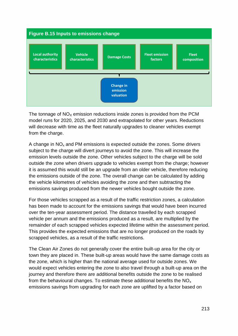
213
Figure B.15 Inputs to emissions change
The tonnage of NOX emission reductions inside zones is provided from the PCM
model runs for 2020, 2025, and 2030 and extrapolated for other years. Reductions
will decrease with time as the fleet naturally upgrades to cleaner vehicles exempt
from the charge.
A change in NOx and PM emissions is expected outside the zones. Some drivers
subject to the charge will divert journeys to avoid the zone. This will increase the
emission levels outside the zone. Other vehicles subject to the charge will be sold
outside the zone when drivers upgrade to vehicles exempt from the charge; however
it is assumed this would still be an upgrade from an older vehicle, therefore reducing
the emissions outside of the zone. The overall change can be calculated by adding
the vehicle kilometres of vehicles avoiding the zone and then subtracting the
emissions savings produced from the newer vehicles bought outside the zone.
For those vehicles scrapped as a result of the traffic restriction zones, a calculation
has been made to account for the emissions savings that would have been incurred
over the ten-year assessment period. The distance travelled by each scrapped
vehicle per annum and the emissions produced as a result, are multiplied by the
remainder of each scrapped vehicles expected lifetime within the assessment period.
This provides the expected emissions that are no longer produced on the roads by
scrapped vehicles, as a result of the traffic restrictions.
The Clean Air Zones do not generally cover the entire built-up area for the city or
town they are placed in. These built-up areas would have the same damage costs as
the zone, which is higher than the national average used for outside zones. We
would expect vehicles entering the zone to also travel through a built-up area on the
journey and therefore there are additional benefits outside the zone to be realised
from the behavioural changes. To estimate these additional benefits the NOx
emissions savings from upgrading for each zone are uplifted by a factor based on
Change in emission valuation
Local authority characteristics
Vehicle characteristics
Fleet emission factors
Fleet composition
Damage Costs

214
the ratio of the zone to built-up area modified by trip length distribution. This uplift
factor is also applied to the congestion benefit for London.
The PCM does not provide estimates of CO2 changes. CO2 emission factors for
different vehicle types and Euro standards are obtained from the Transport Research
Laboratory. There will be a reduction in CO2 emissions as the fleet upgrades to
newer, more fuel-efficient vehicles and a proportion of the fleet is scrapped. From the
data available on number of vehicles, Euro standard and distance travelled; it is
possible to approximate the reduction on emissions due to the upgrade in fleet. It is
also possible to calculate the fuel cost savings using projections of diesel and petrol
prices from DECC151.
B.6 Calculating Net Present Value
For ongoing benefits, a ten-year appraisal period is used from 2020 (when the policy
is assumed to be fully implemented). For analysis purposes, costs incurred with
implementation and upgrading are upfront costs and are assumed to be incurred in
2020. Fuel, NOX, and carbon impacts associated with local measures are incurred
over the ten-year period.
As outlined previously, total benefits include emission damage cost reduction and
fuel savings, while total costs include asset loss, consumer welfare loss and
infrastructure costs.
After obtaining the total quantified cost and benefit figures, the present value of the
differences between the costs and benefits is calculated to provide the NPV
discounted to 2015 prices.
151 Department for Energy and Climate Change, Fossil fuel price projections: 2014,
<www.gov.uk/government/publications/fossil-fuel-price-projections-2014>.

215
Annex C – Theoretical maximum technical potential
C.1 Introduction
To help prioritise and shape the options considered in full in this report, first a high
level assessment was undertaken of the theoretical maximum technical potential
(MTP). The MTP indicates in absolute terms the maximum reduction that could be
expected if a policy was to be implemented at its highest rate. This assessment
does not reflect the technical and implementation challenges in delivering
such an outcome, nor does it provide a full financial impact analysis, but it does
provide an indication of the full potential of different policies to improve NO2
concentrations.
To make such an assessment meaningful it also uses the same indicative
assumptions to calculate the potential costs to Government of such an outcome. In
this way, it can help prioritise and shape the options considered in the full analysis.
The assessment is explained for each option including:
A brief description
An outline of key assumptions
The projected air quality impact
The estimated cost to government
For ease of comparison, the projected air quality impacts have been estimated for
2020 for each option because this is the earliest year of data in the SL-PCM model
that has been used to model these impacts. A summary of the results of the
theoretical maximum technical potential assessment for each of the shortlisted
options is presented in Table 3.8 of the technical report.
C.2 Clean Air Zones
A Clean Air Zone (CAZ) is a geographically defined area bringing together
immediate action to improve air quality. CAZs can include a charging element for
vehicles which enter a CAZ but that do not meet the required standard. To consider
the maximum technical potential of CAZs, the following hypothetical scenario has
been investigated:
All vehicles will be restricted within each CAZ (equivalent to Class D under the
2015 Plan)

216
CAZs are implemented in 27 zones in 2020.
The impact on ambient NO2 concentrations has been modelled in the five
most polluted cities within the UK, which are expected to exceed the legal
limits for NO2 in 2020.
Assuming the mean of these five cities is the representative mean of all non-
compliant cities, the impact on emissions was scaled up to estimate the total
impact of implementation across all the cities. This assumption will be refined
for the final Plan based on assessment of feasible zone perimeters.
London implements the Ultra-Low Emission Zone (ULEZ), while also
tightening restrictions in the wider London area to the same extent.
As with all the options, this is a theoretical assessment to understand the maximum
technical potential and does not incorporate consideration of deliverability. Sections
4-6 describe the options that have been analysed fully.
Air quality impacts
It is estimated that this option will reduce NO2 concentrations by an average of
11.0μg/m3 and emissions of NOx by 29,000 tonnes (51,000 tonnes within the
zones152).
Government cost
Costs to government will be around £595m. This includes the costs to government of
setting up and running the 27 CAZs over a ten-year period.
Table C.1: Maximum technical potential impact of CAZs
Impact Result
AQ impact 11.0µg/m3 reduction
Government cost £600m
152 The reduction within zones is partially offset by increases outside the zones because some
journeys lengthen to avoid the zone

217
C.3 Retrofit
Retrofitting vehicles can reduce the amount of NOx emitted. This policy considers
retrofit schemes for buses, HGVs, and black taxis. The maximum technical potential
scheme assumes that all pre-Euro 6 buses, black cabs, and HGVs will be retrofitted.
Retrofit installs two technologies: selective catalytic reduction (SCR) for buses and
HGVs, and Liquid Petroleum Gas (LPG) retrofit for taxis. SCR is the technology used
in the latest Euro 6 buses and HGVs to minimise NOx emissions. LPG retrofit for
black taxis has been undertaken within the clean vehicle technology fund (CVTF).
The evaluation evidence suggests that emissions after retrofit are equivalent to a
petrol engine.
The assessment for the retrofit measure was carried out using the
Scrappage/Retrofit model.
Air quality impacts
The maximum technical potential option estimates the impact of retrofitting all pre-
Euro 6 buses, black cabs, and HGVs at an average reduction of 1.5µg/m3 in
concentrations of NO2 in 2020. This would result in around 70 percent of taxis, 50
percent of HGVs and 60 percent of buses (around 300,000 vehicles in total) being
retrofitted in 2018.
Government cost
The total cost to Government is estimated at £4,500m to retrofit all vehicles. We
have not estimated the costs of administering the scheme at this stage. Based on
similar schemes these costs are unlikely to be significant in comparison to the costs
of retrofitting vehicles, and therefore excluding these is unlikely to materially affect
the conclusions.
Government is assumed to incur the full cost of retrofit, estimated at £4,500m. The
modelled costs of retrofit are as follows:
Cost of SCR: £17,000
Cost of LPG: £8,000
Costs have been estimated based on existing retrofit schemes undertaken by
Government. The cost of retrofitting HGVs is assumed to be the same as the cost for
retrofitting buses. Total costs were estimated by multiplying the cost of retrofit by the
number of vehicles retrofitted. The modelling assumes that all retrofit takes place in
2018 for the MTP option.

218
Table C.2: Maximum technical potential impact of retrofit
Impact Result
AQ impact 1.5µg/m3 reduction
Government cost £4,500m
C.4 Scrappage
This option estimates the impact of scrapping all pre-Euro 6 diesel cars and vans in
2019. It is limited to diesel vehicles because they emit substantially more NO2 than
petrol vehicles. The hypothetical scenario modelled is that:
Around eight million diesel cars will be scrapped and replaced with new Euro
6 cars.
Around two million diesel vans will be scrapped and replaced with new Euro 6
diesel vans.
As with all the options, this is a theoretical assessment to understand the maximum
technical potential of scrappage and does not incorporate consideration of
deliverability. Sections 4-6 describe the options that have been analysed fully.
A scrappage scheme is expected to improve air quality by increasing fleet turnover
and therefore reducing the average age of the vehicle fleet.
Air quality impacts
The maximum potential option illustrates the potential first order impacts of scrapping
all pre-Euro 6 cars and vans (around ten million vehicles) and replacing them with
new Euro 6 vehicles. The condition on the replacement for this option is a new Euro
6 vehicle, the modelling has assumed that it is equally likely that cars will either be
replaced by diesel or petrol Euro 6 vehicles, and that vans will likely be replaced with
a new diesel Euro 6 vehicle on the basis that diesel vans dominate the market.
It is estimated that there could be around 35 million cars and vans on the road in
2019. The option modelled could result in around 30% of the total stock (of cars and
vans) or around 60% of the total diesel stock (of cars and vans) being scrapped and
replaced with a newer vehicle (Euro 6).
The modelling suggests that this measure could reduce NO2 concentrations by
6.3μg/m3 in 2020. However, it is important to note that this policy could lead to an
increase in average NO2 concentrations of 1.1μg/m3 by 2030. This is because a
scrappage scheme in 2019, by bringing forward the replacement of the oldest
vehicles in the fleet, would mean a spike in the purchase of current Euro 6 vehicles.
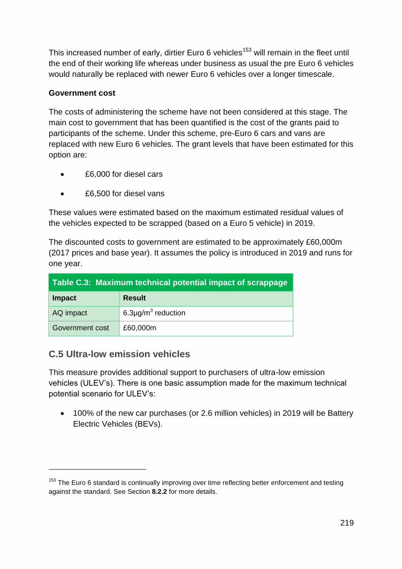
219
This increased number of early, dirtier Euro 6 vehicles153 will remain in the fleet until
the end of their working life whereas under business as usual the pre Euro 6 vehicles
would naturally be replaced with newer Euro 6 vehicles over a longer timescale.
Government cost
The costs of administering the scheme have not been considered at this stage. The
main cost to government that has been quantified is the cost of the grants paid to
participants of the scheme. Under this scheme, pre-Euro 6 cars and vans are
replaced with new Euro 6 vehicles. The grant levels that have been estimated for this
option are:
£6,000 for diesel cars
£6,500 for diesel vans
These values were estimated based on the maximum estimated residual values of
the vehicles expected to be scrapped (based on a Euro 5 vehicle) in 2019.
The discounted costs to government are estimated to be approximately £60,000m
(2017 prices and base year). It assumes the policy is introduced in 2019 and runs for
one year.
Table C.3: Maximum technical potential impact of scrappage
Impact Result
AQ impact 6.3µg/m3 reduction
Government cost £60,000m
C.5 Ultra-low emission vehicles
This measure provides additional support to purchasers of ultra-low emission
vehicles (ULEV’s). There is one basic assumption made for the maximum technical
potential scenario for ULEV’s:
100% of the new car purchases (or 2.6 million vehicles) in 2019 will be Battery
Electric Vehicles (BEVs).
153 The Euro 6 standard is continually improving over time reflecting better enforcement and testing
against the standard. See Section 8.2.2 for more details.

220
This would mean around five million new BEV purchases over three years, this
estimate includes a ramp up period up until 100per cent take-up is achieved in 2019.
Given the current incentive structure, and the additional cost of an average BEV
above a conventional car, the baseline scenario is that most of these 2.6 million
vehicles in 2019 would have otherwise been newly purchased conventional cars
(Euro 6 standard), split equally between petrol and diesel variants.
Air quality impacts
As BEVs have zero emissions, the air quality improvements stem from the
assumption that each additional BEV is replacing a conventional car. Therefore, the
total level of emission reduction from this policy is equal to the total emissions
generated by those five million vehicles being replaced (over the three-year period).
This measure is estimated to reduce NO2 concentrations by an average of
2.99µg/m3 in 2020.
Government cost
For this scenario, the cost to Government is the value of the grants that would be
required to incentivise car buyers to purchase these five million BEV’s. To
understand the potential cost it has been assumed that, in order to get all car buyers
to convert to BEVs, the government would have to pay the full price differential
between a Euro 6 vehicle and a BEV.
These grants would be paid as the BEVs are purchased over the next three years
and the minimum discounted costs would be around £90,000m.
Table C.4: Maximum technical potential impact of ULEVs
Impact Result
AQ impact 2.99µg/m3 reduction in 2020
Government cost £90,000m
C.6 Speed limits
COPERT speed emission curves suggest that vehicles travelling at higher average
speeds should emit more NOx the faster they go (Fig. 6.1 of the technical report).
Different engine types and standards produce different emission speed curves so the
optimum speed (from a NOx perspective) is different for each type of vehicle. Table
C.5 shows that it is not possible to define a single optimum speed limit for all vehicle
types.
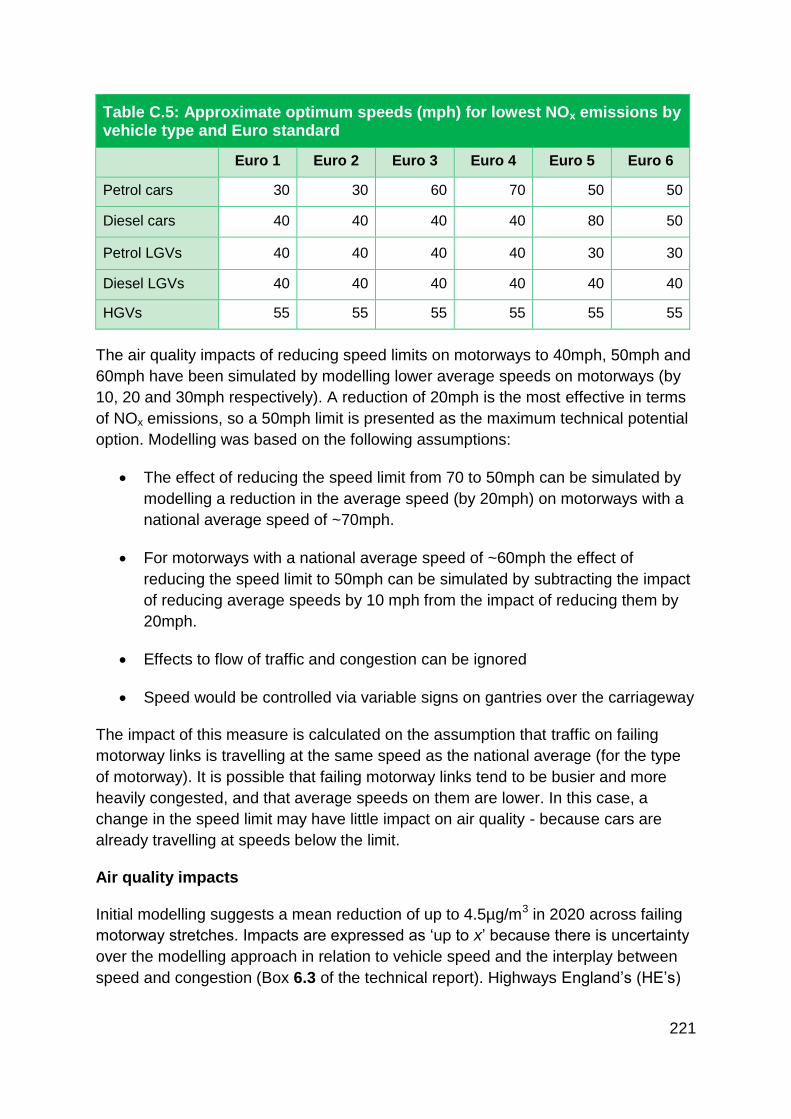
221
Table C.5: Approximate optimum speeds (mph) for lowest NOx emissions by vehicle type and Euro standard
Euro 1 Euro 2 Euro 3 Euro 4 Euro 5 Euro 6
Petrol cars 30 30 60 70 50 50
Diesel cars 40 40 40 40 80 50
Petrol LGVs 40 40 40 40 30 30
Diesel LGVs 40 40 40 40 40 40
HGVs 55 55 55 55 55 55
The air quality impacts of reducing speed limits on motorways to 40mph, 50mph and
60mph have been simulated by modelling lower average speeds on motorways (by
10, 20 and 30mph respectively). A reduction of 20mph is the most effective in terms
of NOx emissions, so a 50mph limit is presented as the maximum technical potential
option. Modelling was based on the following assumptions:
The effect of reducing the speed limit from 70 to 50mph can be simulated by
modelling a reduction in the average speed (by 20mph) on motorways with a
national average speed of ~70mph.
For motorways with a national average speed of ~60mph the effect of
reducing the speed limit to 50mph can be simulated by subtracting the impact
of reducing average speeds by 10 mph from the impact of reducing them by
20mph.
Effects to flow of traffic and congestion can be ignored
Speed would be controlled via variable signs on gantries over the carriageway
The impact of this measure is calculated on the assumption that traffic on failing
motorway links is travelling at the same speed as the national average (for the type
of motorway). It is possible that failing motorway links tend to be busier and more
heavily congested, and that average speeds on them are lower. In this case, a
change in the speed limit may have little impact on air quality - because cars are
already travelling at speeds below the limit.
Air quality impacts
Initial modelling suggests a mean reduction of up to 4.5µg/m3 in 2020 across failing
motorway stretches. Impacts are expressed as ‘up to x’ because there is uncertainty
over the modelling approach in relation to vehicle speed and the interplay between
speed and congestion (Box 6.3 of the technical report). Highways England’s (HE’s)

222
approach would not give a reduction in NO2 concentrations or congestion following
speed limit reduction.
Government cost
Costs for upgrading and operating 45km of motorway, to cover every section of
motorway projected to be in NO2 exceedance in 2020, have been estimated based
on advice from HE.
Costs for installing and maintaining the equipment on the motorway links projected to
be in exceedance in 2020 (about 48km) are estimated to have a 10 year NPV cost of
about £60m. These estimates are based on a high-level average unit cost for the
equipment and its maintenance. They should not be used to develop a standard cost
for every scheme. It is also likely to be an underestimate, as it does not include the
cost of software maintenance and other sundry costs.
Table C.6: Maximum technical potential impact of speed limits
Impact Result
AQ impact Up to 4.5µg/m3 reduction in 2020
Government cost £60m
C.7 Government vehicles
Adherence to Government Buying Standards for transport (GBS-T) is mandatory for
central government. Currently, air quality impacts are not included in the standards.
This policy measure would involve updating GBS-T to include air quality impacts.
Updating the GBS-T for central government would be relatively straightforward given
it does not require any new legislation but the resulting change in purchasing
behaviour is uncertain. This is because air quality would be one of a number of
factors used to select a new vehicle.
Whilst all Government Buying Standards are mandatory for central government, they
are only a recommendation for the wider public sector. Thus, a change to GBS-T
would not automatically lead to a change in wider public sector behaviour. Defra is
exploring how GBS-T could be rolled out across the wider public sector. At this stage
however, analysis is presented for central government only. The maximum technical
potential scenario is based on the following assumptions:
The modelling inputs used do not vary over the appraisal period.
The vehicles referenced in Section 8.2.1 of the technical report stay
representative of their given segments.

223
The GBS-T would be updated to mandate that all central government new car
purchases will be petrol from 2018.
Air quality impacts
The maximum technical potential of this measure would result in all new vehicle
purchases switching from diesel to petrol. New Euro 6 diesel vehicles emit around 10
times more NOx than new Euro 6 petrol vehicles.
Only cars are included given the uncertainty in the availability of petrol variants of
other vehicle types.
As a result of this measure 23% of the total central government car fleet will be a
Euro 6 petrol car in 2020, 61% in 2025, and 76% in 2027. This leads to a mean NO2
concentration reduction of 0.004µg/m3 in 2020.
Government cost
The maximum technical potential of this measure would have a present value cost to
Government of £5.6m over the appraisal period. This cost reflects the capital
switching cost and running cost, the methodology of which can be found in Section
6.3.4 of the Technical Report.
Table C.7: Maximum technical potential impact of Government vehicles
Impact Result
AQ impact 0.004µg/m3 reduction in 2020
Government cost £5.6m
C.9 Vehicle labelling
Vehicle labelling looks to provide consumers with the information they require in
order to make an informed purchasing decision. Historically air pollution has not
been reflected in vehicle labelling because of the way Euro standards were
introduced. This policy would put air quality information in an easy to understand
labelling scheme for all new vehicles sold.
The maximum technical potential option is based on the following assumptions:
The measure will have some behavioural impact behaviourally ammounting to
a maximum technical potential of a 5% shift in purchasing decisions from new
diesel vehicles to new petrol vehicles. This behavioural impact is what was
judged to be the maximum change that could be seen.
This would impact annually from April 2018.

224
Air quality impacts
As a result of this measure, an additional 0.6% of the national car fleet will be Euro 6
petrol in 2020, 1.6% in 2025, and 1.8% by 2027. This will lead to a mean NO2
concentration reduction of 0.13µg/m3 in 2020.
Government cost
It is assumed that the government cost of implementing this measure is negligible
over the appraisal period.
This is because a review of the labelling system is already funded and the addition of
NOx impacts is considered unlikely to result in additional costs. It is also assumed
that running costs for this scheme will be negligible.
Table C.8: Maximum technical potential impact of vehicle labelling
Impact Result
AQ impact 0.13µg/m3 reduction in 2020
Government cost Negligible
C.10 Influencing driving style
This policy would seek to improve a driver’s style of driving with the aim of reducing
vehicle emissions. Excessive speed, maintaining high engine revolutions, and
accelerating hard are all known to increase fuel consumption as well as NOx
emissions. Through this policy, Government would seek to promote driver training
and best practice in order to reduce NOx emissions.
For the maximum technical potential scenario, it is assumed Government would fund
a programme to train all car and LGV drivers and provide them with telematics (a
device which can be fitted into cars and has the ability to measure how well the car is
being driven) to ensure that they adhere to their training.
Air quality impacts
This scenario is estimated to reduce NO2 concentrations by an average of 4.2μg/m3
in 2020 following the assumptions highlighted in Section 6.4.3 of the technical report.
Government cost
The maximum technical potential of this option would have a present value cost to
government of £5,300m over the appraisal period. This reflects the estimated cost of
training and the cost of installing telematics for all drivers.

225
Table C.9: Maximum technical potential impact of influencing driving style
Impact Result
AQ impact 4.2µg/m3 reduction in 2020
Government cost £5,300m

226
Annex D – Clean Air Zones
D.1 Modelling charging Clean Air Zones
The Government has undertaken modelling of charging Clean Air Zones (CAZs) at a
national level to estimate their possible impacts. This modelling is still subject to
further updating based on newer data.
For the purposes of this modelling, assumptions have been made about the type of
charging CAZ that could be implemented to deliver compliance in the shortest
possible time. In the modelling it is assumed that there will be 27 charging CAZs
(Section 4.3.1), which is felt to be a reasonable assumption given the level of
uncertainty in how exceedances at a local level could translate into numbers of
charging CAZs. While national modelling (Annex L to the draft Plan) shows that more
than 27 local areas are projected to have annual mean NO2 concentration
exceedances in 2020 (the year it is assumed that CAZs are introduced), not all local
areas with persistent exceedances will require a separate charging CAZ. There are
broadly three reasons for this:
Overlap: where it might be possible to address exceedances in multiple local
areas through a single charging CAZ.
Not suitable for a charging CAZ: where a charging CAZ is not possible
because no reasonable alternative routes are available by road. In such
areas, specific local solutions will be needed.
Upcoming development: expected infrastructure changes are expected to
address the exceedance.
D.2 Impact of Clean Air Zones on estimated number of vehicles
Estimates of the potential number of cars regularly entering CAZs have been
produced, based on modelling undertaken for this consultation. These were
produced by forecasting the number of cars owned nationally, identifying the
proportion that would be non-compliant, and then estimating the proportion that
might enter a CAZ area.
The forecast of national cars in 2020 is based upon DfT statistics on the vehicle
stock projected forward using the historic change in stock (using a 5 year rolling
average). The UK car fleet is estimated to be 32m in 2020.
The proportion of non-compliant vehicles uses estimates of the split of the vehicle
stock by Euro standard at a national level used as inputs in the PCM. Because

227
information on Euro standards is not collected these are estimated using DfT
statistics on vehicle ages and information on the introduction dates of Euro
standards. The age mix of the fleet is projected forwards to understand the mix of
vehicles by Euro standard in future years. In total it is estimated that 8.5m cars could
be non-compliant in 2020 (the earliest year that CAZs are expected to be
introduced).
Estimates of the number of cars entering CAZs are then made using GPS data.
GPS data tracks vehicles and can be used to identify the numbers that enter
different local authorities. The data is provided by Trafficmaster. The data
captures the movements of approximately 90,000 cars over the course of a
year.
The number of cars in the dataset that enter the original 5 CAZ areas and the
London ULEZ was based on the existing assumed boundaries produced for
the 2015 Plan.
As no decisions have yet been made on the how many CAZs of each type will
be needed, or what their boundaries would be, this number was then scaled
up to provide an estimate of the number of vehicles that might be expected to
enter an assumed 15 car CAZ areas. This was based on potential CAZ
boundaries in additional cities, to understand the marginal impact of adding
extra cities, which was then scaled up to estimate the number of cars
captured in 15 cities.
Because the Trafficmaster data captures only a sample of cars, this was in
turn scaled up to provide an estimate of the total number of cars affected.
Finally, GPS data is also used to track the number of times that cars enter the
assumed CAZ boundaries. This was used to estimate the proportion of cars that
might enter the assumed 15 CAZ areas more than once a week (estimated as
greater than 51 times per year) and more than once a month (estimated as greater
than 11 times per year).
There is significant uncertainty regarding the number of cars that will be impacted,
due to uncertainty around the number of CAZs, their boundaries, and the number
that will cover cars. Furthermore, there is also uncertainty in the methodology as it
relies on GPS data, which covers only a sample of newer vehicles and may not
accurately reflect vehicles on a national basis. It also does not take account of local
differences in the age of vehicles, or travel patterns. Finally, these calculations only
estimate the number of non-compliant cars that might be expected to enter the areas
where a CAZ may be implemented and do not take account of the behaviour change
that would result from CAZ charging.

228
To reflect this uncertainty a significant range is placed around these estimates, from
-50% to +100% in the estimates of cars that regularly enter the CAZs. Estimates of
the number of cars impacted will be refined for the final Plan. The results of the
assessment are presented in Table D.1.
Table D.1 Cars that enter CAZs regularly (millions)
Low Central High
> 51 times per year 0.6 1.1 2.2
> 11 times per year 1.1 2.2 4.4
These numbers have been compared to the number of cars registered in local
authorities that could be affected by car CAZs. DfT publishes vehicle registration
data which, following the approach set out above, has been forecast forward to 2020
and limited to those that would be non-compliant. In total, it is estimated that in 2020
there could be 0.8m non-compliant cars registered in local authorities in England that
could have charging CAZs.
As the CAZ areas would be smaller than the area covered by the local
authority this estimate does not represent the number of registered cars within
CAZs: some of the cars included may never enter CAZ areas.
Many cars that are registered in other local authorities will enter CAZs, so this
should not be used as an estimate of the number of cars affected.
The estimate does not capture the frequency with which cars would enter
CAZs.

229
Annex E – Guidance on calibrated uncertainty language from the Intergovernmental Panel on Climate Change
E.1 Introduction
Following the Air Quality Review group meeting on 2nd March 2017 (Annex F), it was
recommended that the Technical Report should assess and present uncertainties in
line with Intergovernmental Panel on Climate Change (IPCC) guidance. In order to
characterise key findings, calibrated uncertainty language should be used that
conveys the most information to the reader. As per the commitment made in Section
9.1.3, work is ongoing to adopt an approach in line with the IPCC’s guidance154.
The following section explains the criteria used in the IPCC guidance to help
determine how to present uncertainty, recognising that in all cases traceable
accounts of relevant evidence and agreement should be included when describing
uncertainties.
E.2 Criteria used by the IPCC
If a variable is ambiguous, or the processes determining it are poorly known or not
amenable to measurement: confidence should not be assigned; summary terms
should be assigned instead for evidence and agreement (Fig. 9.2). The governing
factors, key indicators, and relationships should also be explained. If a variable could
be either positive or negative, the pre-conditions or evidence for each should be
described.
If the sign of a variable can be identified but the magnitude is poorly known:
Confidence should be assigned when possible (Table 9.3); otherwise summary
terms for evidence and agreement should be assigned. The basis for this confidence
evaluation and the extent to which opposite changes would not be expected should
also be explained
If the order of magnitude can be given for a variable: confidence should be assigned
when possible; otherwise, summary terms for evidence and agreement should be
assigned. The basis for estimates and confidence evaluations made should be
explained, and any assumptions should be indicated. If the evaluation is particularly
154 Mastrandrea, M.D. et al., ‘Guidance Note for Lead Authors of the IPCC Fifth Assessment Report
on Consistent Treatment of Uncertainties’ (2010) Intergovernmental Panel on Climate Change
<https://www.ipcc.ch/pdf/supporting-material/uncertainty-guidance-note.pdf>.

230
sensitive to specific assumptions, then the confidence in those assumptions should
also be evaluated.
If a range can be given for a variable, based on quantitative analysis or expert
judgement: likelihood or probability for that range should be assigned when possible;
otherwise only confidence should be assigned. The basis for the range given should
be explained, noting factors that determine the outer bounds. Any assumptions
made should be stated and the role of structural uncertainties should be estimated.
The likelihood or probability for values or changes outside the range should be
explained, if appropriate.
If a likelihood or probability can be determined for a variable, for the occurrence of an
event, or for a range of outcomes (e.g. based on multiple observations, model
ensemble runs, or expert judgment): a likelihood for the event or outcomes should be
assigned, for which confidence should be “high” or “very high”. In this case, the level
of confidence need not be explicitly stated. Any assumptions made should be stated
and the role of structural uncertainties should be estimated. Characterizing the
likelihood or probability of other events or outcomes within the full set of alternatives,
including those at the tails should be considered.
If a probability distribution or a set of distributions can be determined for the variable
either through statistical analysis or through use of a formal quantitative survey of
expert views: the probability distribution(s) should be graphically presented and/or a
range of percentiles of the distribution(s) should be provided, for which confidence
should be “high” or “very high. In this case, the level of confidence need not be
explicitly stated. The method used to produce the probability distribution(s) and any
assumptions made should be explained, and the role of structural uncertainties
should be estimated. Quantification of the tails of the distribution(s) should be
provided to the extent possible.

231
Annex F – Report on the outcomes of the Air Quality Review meeting
F.1 Introduction
An Air Quality Review meeting was held on 2nd March 2017. Chaired by Defra’s
Chief Scientific Adviser Professor Ian Boyd and attended by the members of the
technical review group including independent academic experts155, this meeting
sought to review the draft technical report that would be published alongside the
draft Plan. This annex sets out the comments and recommendations provided in the
meeting. These have been addressed as far as possible in this technical report, and
will continue to be considered for the final Plan.
F.2 Structural comments
The document presented to the technical group was structured as follows:
Introduction and the challenges.
Air quality assessment and national monitoring network and projections for
concentrations as far as the model can go.
How to make improvements: identifying options available, describing how
these options have been assessed and assessing theoretical maximum
technical potential without any constraints.
Based on this, theoretic potential feasible options were developed. The next three
sections provide more detailed assessments of each of these options split into three
groups
Implementation of Clean Air Zones (CAZs)
National CAZ supporting measures; intended to be targeted in areas where a
CAZ is required to aid the transition.
155 Attendees: Professor Ian Boyd (Chair, Department for Environment, Food and Rural Affairs),
Professor Frank Kelly (Kings College London), Professor Paul S Monks (University of Leicester),
Professor Charles Godfray (Science Advisory Council), Professor Phil Blythe (Department for
Transport). Apologies: Professor Chris Whitty (Department of Health), Professor Sir Mark Walport
(Government Chief Scientific Adviser), Professor Angela McLean (University of Oxford).

232
National measures to supplement CAZs either by targeting different sources
or by operating in different areas.
Distributional analysis, assessing how different groups are affected by the
feasible options.
Sensitivities and uncertainties assessing, and where possible quantifying, the
range around the estimates.
Future steps - how do we improve air quality including finalising the plan and
the wider interests in air quality beyond NO2.
Summary of all the results for potential measures to address NO2.
Following the presentation of this structure, comments were sought. In summary
these were:
The process of describing technical potential then narrowing to potential that
is possible may lose the focus and the attention of reader.
Theoretical maximum might be confusing and we need to be realistic about
actual real life reductions. Also during the movement from theoretical to
practical, the definition of practical is unclear.
o Practicality could be judged on economics, social, political, technical
aspects.
It was clarified that the selection of the technically feasible
option had been defined through collaboration between the
policy and evidence teams.
The document should seek to better clarify and define jargon in order to make
it more accessible.
The document should avoid making a judgement of political sensibilities, as
this was the role of the draft Plan. If necessary, a summary of why technical
options may not be politically acceptable sourced from the covering document
would be a better course of action.
Whilst it is understandable that given the scope of the document the main
focus will be on a single pollutant, this should not limit the scope of the
assessment. A better course of action would be to include considerations of
the effects of other pollutants and potential co-benefits possibly within the
introduction and conclusion.

233
o It was noted that undertaking a multipollutant analysis would not be
expected to substantially change the order of the options. It was also
noted that this multipollutant analysis is expected for the next stage of
the analysis.
Regarding the overall structure, it was concluded that this should be largely
unchanged but there should be an extended executive summary that could
stand alone.
There should be a clear distinction between CAZ measures, national
measures, and supporting measures.
F.3 Comments on uncertainties and presentation
Comments were also sought regarding uncertainties and the presentation of data,
charts, and graphs. The responses were:
It was noted that the technical report included the best available evidence and
one of the biggest challenges is to understand and narrate the uncertainty.
Given this challenge, it was recommended that vocabulary with regards to
uncertainty should be consistent and form a narrative, using the IPCC method
with expert assessment of uncertainty as an example.
It was noted that error bars can be a spurious exercise when error is not
quantitative or meaningful. It is essential the narrative of uncertainty is strong
throughout the document. This means that where figures are quoted the
uncertainty should be explicitly identified. This also means that where trends
are suggested, (for example ‘can increase’) a measure such as ‘is likely to
increase’ should be used where possible.
Uncertainty in the document with regards to the measurement system,
modelling, and cost-benefit analysis should be recognised upfront. It should
also be noted what has been completed to minimise uncertainty, for example
the models tested are the best model available. To deal with each aspect of
uncertainty a table explaining where the uncertainty comes from could be
presented at the beginning of the report.
Graphs and figures should be as clear and transparent as possible. Where
applicable, figures should have an R squared value, n value, and explanation
of where the data points have come from.
The terminology used regarding electric vehicles should be consistent and
clear.
234
It was reflected that a number of options that are widely suggested are not
present for good reason, such as NOx eating paint.
It should also be noted that a key assumption in this modelling is that current
vehicle emission standards deliver the expected reduction in emissions over
time.
F.4 Comments on monitoring and evaluation of the effectiveness of future air quality policies
Finally, comments were sought regarding the monitoring and evaluation of the
effectiveness of future air quality policies. The responses were:
Given the presence of uncertainty, the report should articulate the fact that
work will be conducted in the near future to investigate the national monitoring
system.
The principles of the monitoring system should be outlined in the technical
report; however, details of the monitoring system and evaluation should be
developed by another group.
The principles of the monitoring system should enhance the measurement
strategy prior to the introduction of these policies to provide a baseline. Focus
of monitoring could be CAZs and the surrounding areas.
o It is noted that CAZs will be variable with different geographies and
networks, and so multiple representative CAZs should be measured.
It was suggested that to get a reasonable baseline we should look to get the
new monitoring system operational around 12 months before the policies are
active.
It was also agreed that it was necessary for the new monitoring network to be
operated nationally rather than locally. This creates independence between
the operator and the reviewer, addressing the need to monitor in areas that do
not take action (as controls on the results).
It was also suggested that personal monitoring (otherwise known as exposure
modelling) was in the longer term an important part of the picture especially in
considering the health impacts.

235
F.5 Closing comments
This is the start of the process rather than a single meeting. Written comments from
an independent objective perspective would be valued before the document was
opened for consultation. During the consultation period, another meeting could be
convened. The panel also accepted that it was useful to document and include this
process within the documents including a brief summary of this session.

236
Annex G – Reporting zone NO2 concentrations
Table G.1 Average annual concentration of NO2 on the highest road link in each reporting zone (µg/m3)I Zone name 2017 2018 2019 2020 2021
London 103 96 90 84 78
West Midlands Urban Area 60 59 58 57 54
Greater Manchester Urban Area 52 50 48 46 44
West Yorkshire Urban Area 60 59 59 58 55
Tyneside 54 52 50 48 45
Liverpool Urban Area 47 45 44 42 40
Sheffield Urban Area 53 50 48 45 43
Nottingham Urban Area 57 55 53 51 48
Bristol Urban Area 50 47 45 42 40
Leicester Urban Area 46 45 45 44 43
Portsmouth Urban Area 50 47 45 43 41
Teesside Urban Area 60 56 51 47 45
The Potteries 52 49 45 42 40
Bournemouth Urban Area 45 44 42 41 39
Reading/Wokingham Urban Area 45 44 42 41 40
Coventry/Bedworth 48 46 43 40 38
Kingston upon Hull 47 44 40 36 34
Southampton Urban Area 57 54 51 48 46
Birkenhead Urban Area 42 40 38 36 35
Southend Urban Area 51 49 47 46 43
Glasgow Urban Area 61 56 51 46 44
Edinburgh Urban Area 45 43 42 40 38
Cardiff Urban Area 49 47 46 44 42
Swansea Urban Area 44 43 42 41 38
Belfast Metropolitan Urban Area 51 48 45 41 40
Eastern 54 53 52 50 47
South West 47 45 44 42 40
South East 52 50 47 45 43
East Midlands 57 55 53 51 48
North West & Merseyside 58 55 52 48 46
Yorkshire & Humberside 52 50 48 45 43
West Midlands 53 50 48 45 43
North East 53 51 49 46 44
Central Scotland 45 43 42 40 38
North East Scotland 45 43 40 38 37
South Wales 56 54 52 50 47
North Wales 49 46 44 41 39
Note: results in bold indicate concentrations that are above average annual NO2 limits I Only reporting zones that are projected to be in exceedance of the NO2 limit in 2020 are shown
237
The air quality modelling from the Streamlined PCM model estimates the average
annual NO2 concentration for over 9,000 road links in the UK. The links with the
highest average annual concentration in each reporting zone are then used to
determine which zones are in compliance with annual NO2 concentration limits.
Compliance is therefore determined on a zone-by-zone basis.
Table G.1 shows the reporting zone-level baseline projections for non-compliant
zones from 2017-2021 if no further action is taken. This allows for a comparison to
be made between the highest average annual concentration in each reporting zone
and the expected improvement in concentrations as a result of each of the options
set out in this report.
This comparison suggests that Clean Air Zones (CAZs, Section 4.3 of the Technical
Report) are the only option that is able to deliver concentration improvements
substantial enough to bring reporting zones into compliance within the time period
shown. CAZs are therefore important in bringing about compliance with air quality
limits in the shortest time possible. While the option of lowering speed limits (Section
6.2 of the technical report) could also bring about substantial concentration
improvements, it is only able to do so on motorways. Because of this, only the
Swansea Urban Area could be brought into compliance by the speed limits option in
isolation.

238
Annex H – Assessment of methodologies for interpolating trends in NO2 concentrations for non-modelled interim years
Defra’s air quality modelling currently produces concentration outputs for 2020, 2025
and 2030, and baseline concentration data is available for 2015. However, the
concentrations for the years between these dates need to be estimated in order to
determine which options bring areas into compliance in the shortest time possible.
For the option analysis in this report, the concentration values for interim years have
been estimated though a linear interpolation between the modelled years.
Interpolation is a method of estimating values between a known set of values. In this
case, the values at five-year intervals were known so the values for other years had
to be interpolated from these.
In order to test the accuracy of this approach, baseline NOx emissions data (which is
available for all interim years) has been compared with linear interpolation estimates
for the NOx emissions data in interim years (Figure H.1). This is because it is
assumed that the trend for emissions of NOx is broadly the same as the trend for
mean annual concentrations of NO2. The correlation coefficient between these two
results is 0.998. This indicates that the linear interpolation methodology gives values
that are very close to the true values. Another key finding of this comparison is that
interpolating interim values leads to an overestimation for values between 2020 and
2025, which is the key period in which the majority of zones are estimated to become
compliant. This methodology can therefore be considered to be conservative as it is
likely to slightly overestimate the number of roads that are non-compliant in the years
2020-2025.

239
Figure H.1: UK baseline emission projections: all years compared to five year
intervals with interim years estimated by a linear interpolation (kt NOx)
The accuracy of the linear interpolation methodology has also been tested by
comparing against alternative methodologies for drawing lines of best fit between
data points. Three estimates for interim year values have been calculated: a linear
function, a square polynomial function, and a cubic polynomial function. The results
of these methodologies are shown in Figures H.2, H.3, and H.4.
0
20
40
60
80
100
120
2015 2016 2017 2018 2019 2020 2021 2022 2023 2024 2025 2026 2027 2028 2029 2030
NO
xe
mis
sio
ns (
kto
nn
es)
Year
Emissions baseline Emissions baseline for 5 year intervals with interpolated interim years

240
Figure H.2: UK baseline emission projections: all years compared to five year intervals with interim years estimated using a linear line of best fit interpolation (kt NOx)
Figure H.3: UK baseline emission projections: all years compared to five year intervals with interim years estimated using a square polynomial line of best fit interpolation (kt NOx)
0
20
40
60
80
100
120
2015 2016 2017 2018 2019 2020 2021 2022 2023 2024 2025 2026 2027 2028 2029 2030
NO
xe
mis
sio
ns (
kto
nn
es)
Year
Emissions baseline Linear line of best fit
0
20
40
60
80
100
120
2015 2016 2017 2018 2019 2020 2021 2022 2023 2024 2025 2026 2027 2028 2029 2030
NO
xe
mis
sio
ns (
kto
nn
es)
Year
Emissions baseline Square polynomial line of best fit

241
Figure H.4: UK baseline emission projections: all years compared to five year intervals with interim years estimated using a cubic polynomial line of best fit interpolation (kt NOx)
Of these three alternative methodologies, only the cubic polynomial interpolation
gives a more precise estimate than interpolating the interim years with a correlation
coefficient to the actual baseline of 0.999 (Table H.5). Consequently, the linear
interpolation methodology has been preferred for this report because it gives
estimates that are likely to be extremely close to the actual values, and also gives a
conservative estimate in the key years. The minor improvement in accuracy resulting
from using a cubic polynomial function to interpolate interim years is not considered
to be proportionate given the extra time required to calculate interim year values
using this methodology.
0
20
40
60
80
100
120
2015 2016 2017 2018 2019 2020 2021 2022 2023 2024 2025 2026 2027 2028 2029 2030
NO
xe
mis
sio
ns (
kto
nn
es)
Year
Emissions baseline Cubic polynomial line of best fit

242
Table H.5: Correlation between the modelled emissions estimates for all years and the estimates for emissions in interim years from four potential methodologies
Correlation coefficients
Interpolation
of interim
years
Linear line
of best fit
Square
polynomial
line of best
fit
Cubic
polynomial
line of best
fit
Total correlation to
modelled emissions 0.998 0.994 0.996 0.999
Correlation to modelled
emissions for 2015-19 0.988 0.988 0.986 0.999
Correlation to modelled
emissions for 2020-24 0.997 0.997 0.998 0.997
Correlation to modelled
emissions for 2025-2029 0.997 0.997 0.998 0.999
It should be noted that estimating the concentration values in interim years will not
be necessary for the final Plan because the SL-PCM model will be updated to
generate additional outputs for these years
.

243
Annex I – Glossary of terms
Table I.1 : Table of terms
Term Expanded form Description
ANPR Automatic Number
Plate Recognition
A technology used to automatically recognise
vehicle number plates from a camera image
AURN Automatic Urban and
Rural Network
A network of automatic air quality monitoring
stations measuring oxides of nitrogen (NOx),
sulphur dioxide (SO2), ozone (O3), carbon
monoxide (CO) and particulate matter (PM10, PM2.5)
BCR Benefit-Cost Ratio
An option’s present benefits divided by its present
costs. A ratio that is more than one represents an
option with a positive net present value. A useful
tool for comparing between different projects with
different scales
BEIS
Department for
Business, Energy and
Industrial Strategy
Government department responsible for business,
energy, and industrial strategy.
BEV Battery Electric
Vehicle Vehicles powered by an internal battery
CAZ Clean Air Zone
A policy designed to address areas of poor air
quality. Within a localised geographical zone,
clean-air initiatives will be encouraged and high-
polluting vehicles may have to pay a charge.
CNG Compressed Natural
Gas
Methane gas stored at high pressure and a fuel
that can be used in place of petrol, diesel, and
liquefied petroleum gas.
COPERT
Computer Programme
on Emissions from
Road Transport
A computer program financed by the European
Environment Agency to calculate the emissions of
pollutants from road transport.
COPERT 5
Computer Programme
on Emissions from
Road Transport 5
The fifth and latest update of COPERT.
DECC Department of Energy
and Climate Change
Former governmental department responsible for
energy and climate change, now part of BEIS

244
DfT Department for
Transport Governmental department responsible for transport
DPF Diesel Particle Filter A device to remove particulate matter or soot from
the exhaust gas of a diesel engine.
EV Electric Vehicle Vehicles powered by electricity, includes both
hybrid and battery electric vehicles
FAM Fleet Adjustment
Model
The Fleet Adjustment Model quantifies the societal
costs and benefits associated with changes in UK
vehicle fleet
GBS Government Buying
Standards
A procurement standard used by all central
government departments and their related
organisations when buying goods and services for
those product groups covered. The mandatory
standards are encouraged for the wider public
sector to specify in tenders.
GIS Geographical
Information System
A computer system for capturing, storing,
analysing, and displaying data related to positions
on Earth’s surface.
HE Highways England
The government company charged with operating,
maintaining and improving England’s motorways
and major A roads, formerly the Highways Agency
HGVa Articulated Heavy
Goods Vehicles
Tractor units with a semi-trailer attached where part
of the load is borne by the drawing vehicle
HGVr Rigid Heavy Goods
Vehicles Heavy goods vehicles without a trailer attached
HGVs Heavy Goods
Vehicles
Larger vehicles constructed for transporting goods.
Must have a gross weight more than 3.5 tonnes.
This includes road tractors and curtain sided
vehicles (with a gross weight of over 3.5 tonnes)
ICCT International Council
on Clean Transport
An independent non-profit organisation founded to
provide first-rate, unbiased research and technical
and scientific analysis to environmental regulators.
ICE Internal Combustion
Engine
An internal combustion engine is a heat engine
where the combustion of a fuel occurs with an
oxidizer (usually air) in a combustion chamber that
is an integral part of the working fluid flow circuit.

245
LGVs Light Goods Vehicles
4-wheel vehicles constructed for transporting
goods. Must have a gross weight of 3.5 tonnes or
less. This includes road tractors and curtain sided
vehicles (with a gross weight of 3.5 tonnes or less)
LowCVP Low Carbon Vehicle
Partnership
A public-private partnership, established in 2003,
that exists to accelerate a sustainable shift to lower
carbon vehicles and fuels and create opportunities
for UK business
LPG Liquefied Petroleum
Gas
Alternative fuel for vehicles, as opposed to diesel or
petrol
NEDC New European
Driving Cycle
The current laboratory test for measuring the level
of CO2 and pollutant emissions from vehicles so as
to compare them against EU regulations. The
standardised testing procedure allows comparison
of emissions between different vehicle models.
NH3 Ammonia
A gas that contributes to the formation of
particulate matter in the atmosphere and can cause
respiratory problems.
NM-VOCs Non-methane volatile
organic compounds
A variety of chemically different organic
compounds, excluding methane, that easily
become vapours or gases.
NO2 Nitrogen Dioxide A respiratory irritant that may cause respiratory
problems and increase susceptibility to infections.
NOx Nitrogen Oxides
A respiratory irritant that may exacerbate asthma
and possibly increase susceptibility to infections.
The nitric oxide (NO) portion can form nitrogen
dioxide in the atmosphere through oxidation.
NPV Net Present Value
A calculation of the differences in the present value
of an option’s cost and benefits streams. The NPV
is the primary criterion for deciding whether
government action can be justified.
NRMM Non-Road Mobile
Machinery
Any mobile machine, item of transportable
industrial equipment, or vehicle - with or without
bodywork - that is: 1. Not intended for carrying
passengers or goods on the road. 2. Installed with
a combustion engine - either an internal spark
ignition petrol engine, or a compression ignition
diesel engine. A generator is an example.
246
O3 Ozone
A respiratory irritant: short-term exposure to high
ambient concentrations can cause inflammation of
the respiratory tract and irritation of the eyes, nose,
and throat.
PCM Pollution Climate
Mapping model
A collection of models designed to fulfil part of the
UK’s EU Directive (2008/50/EC) requirements to
report on the concentrations of particular pollutants
in the atmosphere. It is consistent with the National
Atmospheric Emissions Inventory (NAEI).
PM Particulate Matter A category of particles with a wide range of sizes
and different chemical constituents.
PV Present Value
The cost or benefit of an action in today’s money.
Future costs or benefits are discounted to the base
year using Treasury guidelines
RDE Real Driving
Emissions
A test scenario to determine the emissions of
vehicles in a road environment.
REVIHAAP
Review of evidence
on health aspects of
air pollution
A World Health Organisation document which
presents answers to 24 questions relevant to
reviewing European policies on air pollution and to
addressing health aspects of these policies
SCR Selective Catalytic
Reduction
A means of converting emissions of NOx from a
stream of exhaust gases into water and other
compounds by use of a catalyst
SL-PCM Streamlined-PCM
model
A simplification of the full Pollution Climate
Mapping model.
SO2 Sulphur Dioxide A respiratory irritant that can cause constriction of
the airways.
SRN Strategic Road
Network
Made up of the motorways and major trunk roads in
England that are managed by Highways England, it
comprises approximately 4,400 miles of road.
TfL Transport for London
An integrated transport authority responsible for
delivering the Mayor of London’s strategy and
commitments on transport. Runs the day-to-day
operation of the Capital's public transport network
and manages London's main roads.
TRL Transport Research
Laboratory
An independent transport consultant that provides
innovative research, technology and software
solutions for surface transport modes and related
markets of automotive, motorsport, insurance and
energy

247
UK-AIR UK Air Information
Resource
Defra’s webpages that provide in-depth details on
air quality and air pollution in the UK.
ULEVs Ultra Low Emission
Vehicles
New vehicles with pure electric engines, plug‐in
hybrid engines, or cars with CO2 emissions below
75g/km at the exhaust pipe.
VED Vehicle Excise Duty
An excise duty that must be paid to use a vehicle
on the UK’s public roads. The rate varies based on
the car’s quantity of CO2 emissions.
WHO World Health
Organisation
A specialised branch of the United Nations (UN)
that is concerned with international public health
WLTC
Worldwide
Harmonised Light
Vehicles Test Cycle
A means for determining the emissions and fuel
consumption from light-duty vehicles.